SCHOOL OF ECONOMICS - UNSW Business School · SCHOOL OF ECONOMICS HONOURS THESIS ... Jahanzeb Khan...

1

SCHOOL OF ECONOMICS

HONOURS THESIS

Pass-Through of Exchange Rate Shocks to

Inflation in an Australian Context

Author: Jason Yu

Supervisor: A/Prof. Glenn Otto

Submitted as part of the requirement for the degree of:

B. Commerce (Finance and Financial Economics)/B. Economics

(Economics)

Honours in Economics

22nd

October, 2012

2

DECLARATION

I hereby declare that this thesis is my own original work, and to the best of my

knowledge, it contains no material that has been published or written by other author(s)

except where due contributions been acknowledged. This thesis has not been

submitted to any other university or institutions as part of the requirements for another

degree or other award.

Jason Yu

22 October 2012

3

ACKNOWLEDGEMENTS

In accomplishment of this thesis, I cannot help to think that my achievements were the

fruits of many others' support and encouragement. First and foremost, I would like to

sincerely thank my supervisor Associate Professor Glenn Otto for his tremendous

support and guidance throughout my Honours year. I am extremely grateful for the

time and effort spent to help me accomplish my thesis. Without the guidance of my

supervisor, the construction of this thesis would have been impossible.

I am also indebted to James Morley for his valuable comments and discussions both in

and outside the seminars. I wish to thank Andy Tremayne, Mariano Kulish, Nigel

Stapledon, and Scott French for their helpful comments and advice during the final

seminar. Additionally, I would like to thank the Donors of Australian School of

Business at UNSW for the Honours scholarship, which provided me financial support

throughout the Honours year.

To the Honours cohort 2012: Thank you for all those fun and stressful times spent

together. Also, I wish to thank Josef Manalo for his mentorship in preparation for my

Honours year; Jahanzeb Khan and Anthony Chan for proof-reading my whole thesis;

and Anthony Chan's family for the affordable accommodation. Finally, I would like to

thank Hong Il Yoo for his expertise in microeconometrics.

Last, but certainly not least, thanks goes to my family who continually supported me

both in physical and spiritual ways that provided me strong motive to plough through

the Honours year.

4

TABLE OF CONTENTS

Abstract ....................................................................................................................... 11

1. Introduction ............................................................................................................ 12

2. Literature Review .................................................................................................. 16

2.1 Australian Pass-through Literature ...................................................................... 16

2.2 Partial Equilibrium Approach ............................................................................. 18

2.3 General Equilibrium Approach ........................................................................... 20

2.4 Empirical-based Literature .................................................................................. 22

3. Theoretical Model .................................................................................................. 25

4. Econometric Methodology .................................................................................... 28

4.1 Structural Vector Error Correction Model .......................................................... 28

4.2 Identification Under Weak Exogeneity ............................................................... 30

5. First Stage Pass-through: Exchange Rate to Import Price ................................ 33

5.1 Data Description and Properties .......................................................................... 33

5.2 Model Estimation and Identification ................................................................... 37

5.3 Main Results for First Stage Pass-through .......................................................... 40

5.4 Australian Inflation Targeting Subsample .......................................................... 43

5.5 Rolling Window for Coefficient Stability ........................................................... 48

6. Second Stage Pass-through: Import Price to Inflation ....................................... 49

6.1 Data Description and Properties .......................................................................... 49


6.3 Main Results for Second Stage Pass-through ..................................................... 54

6.5 Australian Inflation Targeting Subsample .......................................................... 58

6.6 Rolling Window for Coefficients Stability ......................................................... 64

7. Combined Stage Pass-through: Exchange Rate to Retail Price ........................ 65

5

7.1 Data Properties .................................................................................................... 65


7.3 Main Results for Combined Stage Pass-through ................................................. 69

7.4 Australian Inflation Target Subsample ............................................................... 73

7.6 Rolling Window for Coefficients Stability ......................................................... 74

8. Conclusion and Limitations .................................................................................. 75

8.1 Conclusion ........................................................................................................... 75

8.2 Limitations and Future Research ......................................................................... 76

Appendix 1: Data Construction ................................................................................ 79

A1.1 Retail Prices of Imported Consumption Goods ................................................ 79

A1.2 Prices of Consumption Imports Over-the-docks .............................................. 81

A1.3 World Export Price for Consumption Goods ................................................... 81

A1.4 Nominal Effective Exchange Rate ................................................................... 85

A1.4 Costs Borne By Importers and Retailers .......................................................... 85

Appendix 2: Reduced-form Level VAR Lag Selection ........................................... 87

Appendix 3: Further Test for Cointegration ........................................................... 91

Appendix 4: Approximate 2 Standard Error Bands Based on Levels VAR ........ 92

Appendix 5: Data Properties and Model Estimation for Subsamples .................. 98

Appendix 6: Impulse Response Functions for Further Robustness Tests .......... 102

Appendix 7: Rolling Window for Coefficient Stability ........................................ 104

Bibliography ............................................................................................................. 105

6

LIST OF TABLES

Chapter 5

Table 5.1: First Stage Augmented Dickey-Fuller Test Results .................................... 36

Table 5.2: First Stage Pass-through Engle-Granger Test Results ................................. 36

Table 5.3: First Stage Pass-through Johansen Cointegration Test Results ................... 36

Table 5.4: First Stage Pass-through Estimation Results ............................................... 36

Table 5.5: First Stage Adjustment Coefficients Implied By Johansen Normalised

Coefficients on Error Correction of VECM(2) ............................................................. 38

Table 5.6: First Stage Variance Decomposition of Permanent and Transitory Shocks

for Full Sample Period .................................................................................................. 42


for Subsample 1983Q2-1993Q1 ................................................................................... 46


for Subsample 1993Q2-2010Q1 ................................................................................... 47

Chapter 6

Table 6.1: Second Stage Augmented Dickey-Fuller Test Results ................................ 52

Table 6.2: Second Stage Pass-through Engle-Granger Test Results ............................ 52

Table 6.3: Second Stage Pass-through Johansen Cointegration Test Results .............. 52

Table 6.4: Second Stage Pass-through Estimation Results ........................................... 52

Table 6.5: Adjustment Coefficients on Error Correction of VECM(2) ........................ 53

Table 6.6: Variance Decomposition of Permanent and Transitory Shocks: Full Sample

Period ............................................................................................................................ 57

Table 6.7: Second Stage Variance Decomposition of Permanent and Transitory Shocks

Implied By DOLS Estimates: 1983Q2-1993Q1 ........................................................... 61

7

LIST OF TABLES (CONT.)

Chapter 6 (Cont.)

Table 6.8: Second Stage Variance Decomposition of Permanent and Transitory Shocks

Implied By DOLS Estimates: 1993Q2-2010Q1 ........................................................... 63

Chapter 7

Table 7.1: Combined Stage Pass-through Estimation Results ...................................... 65

Table 7.2: Combined Stage Pass-through Four-Variables VECM Engle-Granger Test

Results ........................................................................................................................... 66

Table 7.3: Combined Stage Pass-through Four-Variables VECM Johansen

Cointegration Test Results ............................................................................................ 66

Table 7.4: Combined Stage Pass-through Four-Variables VECM Estimation Results 66

Table 7.5: Adjustment Coefficients on Error Correction of VECM(2) ........................ 68

Table 7.6: Combined Stage Variance Decomposition of Permanent and Transitory

Shocks: Full Sample Period .......................................................................................... 72

Table 7.7: Combined Stage Pass-through Subsamples Estimation Results .................. 73

Appendices

Table A1.1: Australia's Major Trading Partner TWI Weights ...................................... 82

Table A1.2: Cost Index Weights ................................................................................... 87

Table A2.1: Level VAR Lag Length Selection Criterions ........................................... 89

Table A2.2: Level VAR Residual Serial Correlation LM Test .................................... 90

Table A3.1: Significance of Error Correction Term Test ............................................. 91

Table A5.1: First Stage Pass-through Estimation Results: 1983Q2-1993Q1 ............... 99

Table A5.2: First Stage Pass-through Adjustment Coefficients on Error Correction of

VECM(2) Implied By DOLS Estimates: 1983Q2 - 1993Q1 ........................................ 99

8

LIST OF TABLES (CONT.)

Appendices (Cont.)

Table A5.3: First Stage Pass-through Estimation Results: 1993Q2 - 2010Q1 ............. 99

Table A5.4: Second Stage Pass-through Estimation Results: 1983Q2 - 1993Q1 ....... 100

Table A5.5: Second Stage Pass-through Adjustment Coefficients on Error Correction

of VECM(2) Implied By DOLS Estimates: 1983Q2 - 1993Q1 .................................. 100


of VECM(2) Implied By Johansen Normalised Coefficients: 1983Q2 - 1993Q1 ...... 100

Table A5.7: Second Stage Pass-through Estimation Results: 1993Q2 - 2010Q1 ....... 101


of VECM(2) Implied By DOLS Estimates: 1993Q2 - 2010Q1 .................................. 101

9

LIST OF FIGURES

Chapter 1

Figure 1.1: Plot of Exchange Rate, Import Price, and Retail Price .............................. 12

Chapter 5

Figure 5.1: First Stage Pass-through Variables ............................................................. 35

Figure 5.2: First Stage Impulse Response for One Standard Deviation Permanent and

Transitory Shocks With Johansen Normalised Coefficient: Full Sample .................... 40

Figure 5.3: First Stage Impulse Response for One Standard Deviation Permanent and

Transitory Shocks With DOLS Estimates: 1983Q2 - 1993Q1 ..................................... 43

Figure 5.4: First Stage Impulse Responses for One Standard Deviation Permanent and

Transitory Shocks With DOLS Estimates: 1993Q2 - 2010Q1 ..................................... 45

Figure 5.5: First Stage Pass-through Rolling Window on DOLS Coefficients ............ 48

Chapter 6

Figure 6.1: Second Stage Pass-through Variables ........................................................ 50

Figure 6.2: Impulse Responses for One Standard Deviation Permanent and Transitory

Shocks With DOLS Estimates: Full Sample ................................................................ 55


Shocks With DOLS Estimates: 1983Q2 - 1993Q1 ....................................................... 58


Shocks With DOLS Estimates: 1993Q2 - 2010Q1 ....................................................... 60

Figure 6.5: Second Stage Pass-through Rolling Window on DOLS Coefficients ........ 64

Chapter 7


Shocks With Johansen Normalised Coefficients: Full Sample..................................... 70

Figure 7.2: Combined Stage Pass-through Rolling Window on DOLS Coefficients ... 74

10

LIST OF FIGURES (CONT.)

Appendices

Figure A4.1: First Stage Pass-through Impulse Response Functions From VAR(3):

Full Sample ................................................................................................................... 93


1983Q2-1993Q1 ........................................................................................................... 93


1993Q2-2010Q1 ........................................................................................................... 94

Figure A4.4: Second Stage Pass-through Impulse Response Functions From VAR(3):

Full Sample ................................................................................................................... 94

Figure A4.5: Second Stage Pass-through Impulse Response Functions From VAR(3)

With Ordering Implied By DOLS Estimates: 1983Q2-1993Q1 ................................... 95


With Ordering Implied By Johansen Normalised Coefficients: 1983Q2-1993Q1 ....... 95


With Ordering Implied By Johansen Normalised Coefficients: 1993Q2-2010Q1 ....... 96

Figure A4.8: Combined Stage Pass-through Impulse Response Functions From VAR(3)

With Ordering Implied By Johansen Normalised Coefficients: Full Sample ............... 97

Figure A6.1: First Stage Pass-through Impulse Response Functions on VECM(2)

Implied By Johansen Normalised Estimates: Full Sample ......................................... 102

Figure A6.2: Second Stage Pass-through Impulse Response Functions on VECM(2)

Implied By DOLS Estimates: Full Sample ................................................................. 103

Figure A6.3: Impulse Responses for One Standard Deviation Permanent and

Transitory Shocks With Johansen Normalised Coefficients: 1983Q2-1993Q1 ......... 103

Figure A7.1: First Stage Johansen Normalised Cointegrating Coefficients ............... 104

Figure A7.2: Second Stage Johansen Normalised Cointegrating Coefficients ........... 104

Figure A7.3: Combined Stage Johansen Normalised Cointegrating Coefficients ...... 104

11

Abstract

This thesis seeks to address the resilience of the import price pass-through to the retail

price (second stage) despite significant pass-through from the exchange rate to the

import price (first stage). Specifically, this "exchange rate puzzle" is addressed by

extending a theoretical mark-up model into a cointegrated vector autoregressive

framework to assess whether the mark-up on input cost plays an increasing role in the

exchange rate pass-through during the past decades. If so, is the decline in the

exchange rate pass-through triggered by inflation targeting?

The main contribution to the previous literature involves the decomposition of

permanent and transitory shocks with structural identification under weak exogeneity

in a system framework, which complements the typical single-equation results seen in

the exchange rate literature.

Three main results are concluded. Firstly, the first stage pass-through confirms the

lack of second stage pass-through is not a result of sluggish response in the first stage.

Secondly, second stage pass-through result is much slower and low in magnitude

compared to the first stage, which suggests the mark-up is increasingly persistent in

conjunction with large fluctuations during the inflation targeting periods. Additionally,

retail price becomes less persistent after the inflation targeting policy, which provided

consistent evidence that inflation targeting triggers these behaviours. Lastly, from the

combined stage pass-through, the direct impact of the exchange rate pass-through on

the retail price is found to be higher than the second stage. Nevertheless, mark-up on

cost is still an important factor in the direct pass-through of exchange rate to the retail

price. Although, the robustness subsample test cannot confirm the results from the

combined stage.

12

1. Introduction

Since the floatation of the Australian dollar during the 1980s, exchange rate shocks

has always been an external shock that influences the domestic inflation levels.

However, with the past two decades of inflation targeting implemented by the Reserve

Bank of Australia (RBA), inflation was kept at a low level in the face of inflationary

pressure derived from fluctuations in the exchange rate during economic booms in the

business cycle.

A recent bulletin article published by Chung et al. (2011) from the RBA described the

recent surge in the exchange rate pass-through to retail price via the imported

consumption channel, particularly for highly tradeable consumption goods. In a mark-

up framework where retail price is in proportion to the import price and the input cost

with an additional mark-up, D'Arcy et al. (2012) provided the fact that "...only half of

the final price of retail goods is attributable to the cost of producing these items. The

other half is the cost of distributing these items...". These two articles highlighted the

importance of cost. Therefore, the mark-up on costs appears to be a key determinant in

the exchange rate pass-through.

Figure 1.1: Plot of Exchange Rate, Import Price, and Retail Price

40

50

60

70

80

90

100

110

120

84 86 88 90 92 94 96 98 00 02 04 06 08

TWI PD RPI

13

From Figure 1.11, during the episodes of depreciation between the late 1984 to mid

1986, the import price over-the-docks shows potential influences over the retail price

of consumption imports2. During the episodes of depreciation occurred in the early

1990s, the retail price seem to be less responsive to changes in import price. In

addition, the announcement of inflation targeting by RBA in mid 1993 marked by the

dashed line seems to have caused retail price to adjust to changes in the import price.

After mid 2002, the response of retail price is insensitive to the episodes of sustained

appreciation, which consequently caused a general decline in the import price.

Particularly, during the height of global financial crisis, retail price is unaffected

despite sharp changes in the import price. Thus, the alighted "exchange rate puzzle"

involve the insensitivity of retail import price in respond to significant movements in

the exchange rate, even though, the response of import price to fluctuations in the

exchange rate is quick and large in magnitude.

Three possible explanations are mentioned by Murray (2008). One possible reason is

due to the claim made by Taylor (2000) who associated the decline in pass-through to

the global stabilisation of inflation. Another reason mentioned is due to changes in

composition of trade. Campa et al. (2005) and related studies unearthed evidence

towards an increase in differentiated manufacture goods caused by an increase in price

discrimination across markets. The last reason is attributed to an increased

globalisation and the role played by emerging countries.

Amongst these reasons, Dwyer and Leong (2001) explained the decline in pass-

through is due to structural change in Australia's inflation process, however, they did

1 TWI = Trade Weighted Index, PD = Imported Price of Consumption Over-the-docks, RPI = Retail

Price of Consumption Goods. 2 Exchange rate, import price over-the-docks, and retail price form the consumption portion of imports

derived from aggregated data. For more details, please refer to Appendix 1: Data Construction.

14

not find a statistically significant result of their claim. Another possibility mentioned

by Dwyer and Lam (1994) is due to the ability of retailers in varying their mark-up on

input costs, thereby, absorbs some of the fluctuations. Particularly, they argue the

tendency of addressing the second stage as being "incomplete" when retail price

responds less than one-for-one with import price over-the-docks.

Despite various theories in response to the exchange rate puzzle proposed in the pass-

through literature, there is still insufficient empirical evidence that evaluates

Australia's exchange rate pass-through to the domestic inflation. This thesis

contributes to the pass-through literature by empirically evaluating the dynamic

relationships of exchange rate shocks and the response to the key domestic variables.

Typically, the main research question that this thesis will address is; does mark-up on

cost of input serve to explain the exchange rate puzzle? If so, is the decline in pass-

through over the recent decades a result of the increasing role played by the mark-up

on costs triggered by the RBA's inflation targeting policy?

In response to the stated research question, there are important implications if mark-up

on cost are found to play a significant role in exchange rate pass-through. Better

understanding of the pass-through to the retail price enables central bank to improve

forecast in future inflation levels, which increase the efficiency in the implementation

of monetary policy aim to control inflation within 2-3% target level in the medium

terms. If shocks are insulated due to a more fluctuating and persistent mark-up, which

prevents the penetration to retail price, then, policy that target exchange rates should

be kept minimum to avoid any adverse consequences on the domestic output.

The pass-through of exchange rate to the retail price is typically decomposed into two

stages. The first stage empirically confirms exchange rate shock does transmit to the

15

import price at a relatively fast speed and significant in magnitude. Consequently, the

research question is addressed in the second stage of pass-through.

Despite the abundance of single-equation framework in the existing literature, a

structural system of linear equations is used instead for each pass-through stage.

Norman and Richards (2010) discussed the drawbacks of single-equation and its

limitations. Clearly, one of the advantages of using a structural model is the ability to

impose certain theoretical restrictions that most economists agree in the long-run.

Additionally, a Structural Vector Error Correction Model (SVECM) has the advantage

in decomposition of key pass-through variables in to permanent and transitory shocks.

The second stage informs us whether the mark-up is important when first stage pass-

through is described as near complete. Second stage results shows the pass-through of

import price to the retail price is extremely, slow and small in magnitude. This implies

that the fluctuations in mark-up are large and persistent in the long-run. However, the

input cost shocks (mark-up) in response to the retail price were not captured in the full

sample due to the shock been transitory.

This drawback motivated the combined stage pass-through in a four-variables SVECM

which directly traces the relationship between the retail price and the exchange rate.

Once the exchange rate (and the world price) is explicitly included into the system, the

response of retail price to input costs is slow and moderate in magnitude. Furthermore,

the response of retail price to exchange rate shock more than doubles in the long-run

equilibrium when compared to the second stage. This reflects the price adjustment to

the changes in the exchange rate directly. In conclusion, varying mark-up plays an

absorptive role which explains the resistance in the pass-through of import price to the

retail price, when pass-through of exchange rate to the domestic import price is high.

16

2. Literature Review

Exchange rate pass-through has been a widely researched area. The theoretical

literature involves two approaches, namely, the partial equilibrium and the general

equilibrium. In this chapter, a brief overview of the Australian experience in pass-

through literature will be explored. This is followed by a section of the two different

approaches. The focus of the literature review is on the exchange rate pass-through to

inflation either via import channel or export channel. Finally, empirical literature is

discussed to shed light on the model identification strategy used in this study.

2.1 Australian Pass-through Literature

A vast body of pass-through literature focus on industrialised economies; however,

there are limited studies in the Australian pass-through literature. This is due to the

unavailability of data that drives the empirical work. For example, a popular proxy

used for controlling demand pressure of the destination country can be difficult to

obtain for Australia. Despite this issue, a few key papers triumph in exploring the

relationship between the pass-through of the exchange rate and either the import price

of particular domestic industry or that of the export price. A widely cited paper written

by Menon (1993) examined the exchange rate pass-through to Australian imported

motor vehicles. The author found the short run pass-through of exchange rate was 70%

and long run pass-through estimated to be 80%. These estimates are slightly higher

compared to that of other industrialised economies.

Despite various studies on the exchange rate pass-through to the imported manufacture

goods prices, both Menon (1992) and Swift (1998) also examined the export price of

Australian manufactured goods in the 1980s. However, Menon (1992) used

disaggregated export dataset for manufactured goods, while Swift (1998) explored the

17

exchange rate pass-through with aggregated exports. Another similarity is the mark-up

analytical framework, which enables retailers to vary their mark-up in response to the

exchange rate shock. Menon (1992) concluded a varying degree of pass-through

effects in different industries. This conclusion is based on complete import price pass-

through with the small country assumption of the Australian economy. Thus, the terms

of trade in the domestic economy is insulated from any changes movements in the

exchange rates. Swift (1998) concluded that in the long run, 60% of the exchange rate

pass-through to the Australian aggregate exports. This conclusion supports Menon

(1992) on the small country assumption for the Australian aggregated exports.

A series of RBA research discussion papers focus on the issue of exchange rate pass-

through via the imported price channel. Dwyer et al. (1993), however, explored the

pass-through effects of exchange rate movements for both imported price and export

price of manufactured traded goods. They also tested the small country assumption for

Australia with the inclusion of second stage pass-through. Menon (1992), Menon

(1993), and Swift (1998) focused their studies solely on the first stage of pass-through3.

In the long run, in comparison to Menon (1993), Dwyer et al. (1993) found the first

stage exchange rate pass-through to be complete and rapid. However, in the short run,

the pass-through effect completes within one year. Furthermore, both studies find a

reduction in the speed of the exchange rate pass-through to exports and detect the

change in pricing patterns.

During the depreciation occurred in the 1990s, Dwyer and Leong (2001) addressed the

question of whether the periods of stable inflation was the result of favourable shocks

to the macroeconomy or was it a fundamental structural change in the Australian

inflation process. Through a mark-up framework, they found statistically insignificant

3 The second stage pass-through to export was not considered by Menon (1993).

18

decline in the speed of adjustment back towards long-run equilibrium. Nevertheless,

they conclude Australia is far from perfect insulation against exchange rate shocks and

any other types of external shocks that are large in magnitude and persistent in nature.

In contrast to the error correction type methodology employed in the Australian

literature, Heath et al. (2004) used Dynamic Ordinary Least Square (DOLS) to

estimate the two pass-through stages in a mark-up framework. They incorporated leads,

lags, and contemporaneous terms for the growth in import price, unit labour cost, and

output gap in the two pass-through stages. Compared to Dwyer and Leong (2001) with

insignificant decline in pass-through, Heath et al. (2004) found that there has been a

large scale decline in the pass-through of exchange rate to the consumer price. This

pattern correlates to the global trend of low and stable inflation environment.

Finally, Dwyer and Lam (1994) focused their attention to the second stage pass-

through. Empirical research in Australia has limited break-through in the second stage

pass-through due to data constraints. However, they shed new light with the

construction of their own costs and margins. They addressed the pass-through in two

stages with a mark-up model estimated on the grounds of Unrestricted Error

Correction Model (UECM). They confirmed that the first stage pass-through for

Australia is complete in the long-run. Furthermore, they concluded that the second

stage was also complete.

2.2 Partial Equilibrium Approach

Partial equilibrium approach has been the main theoretical underpinning of the early

literature in the exchange rate pass-through. This approach has roots that originated

from the Law Of One Price (LOOP). LOOP states that the price of all traded goods

should be the same across all countries when currency is expressed under a common

19

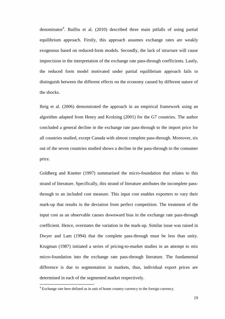
denominator4. Bailliu et al. (2010) described three main pitfalls of using partial

equilibrium approach. Firstly, this approach assumes exchange rates are weakly

exogenous based on reduced-form models. Secondly, the lack of structure will cause

imprecision in the interpretation of the exchange rate pass-through coefficients. Lastly,

the reduced form model motivated under partial equilibrium approach fails to

distinguish between the different effects on the economy caused by different nature of

the shocks.

Ihrig et al. (2006) demonstrated the approach in an empirical framework using an

algorithm adapted from Henry and Krolzing (2001) for the G7 countries. The author

concluded a general decline in the exchange rate pass-through to the import price for

all countries studied, except Canada with almost complete pass-through. Moreover, six

out of the seven countries studied shows a decline in the pass-through to the consumer

price.

Goldberg and Knetter (1997) summarised the micro-foundation that relates to this

strand of literature. Specifically, this strand of literature attributes the incomplete pass-

through to an included cost measure. This input cost enables exporters to vary their

mark-up that results in the deviation from perfect competition. The treatment of the

input cost as an observable causes downward bias in the exchange rate pass-through

coefficient. Hence, overstates the variation in the mark-up. Similar issue was raised in

Dwyer and Lam (1994) that the complete pass-through must be less than unity.

Krugman (1987) initiated a series of pricing-to-market studies in an attempt to mix

micro-foundation into the exchange rate pass-through literature. The fundamental

difference is due to segmentation in markets, thus, individual export prices are

determined in each of the segmented market respectively.

4 Exchange rate here defined as in unit of home country currency to the foreign currency.

20

Marazzi et al. (2005) provided a recent example of pricing-to-market. The purpose

was to maximise profit from the total sum of all markets for a differentiated product

subject to given constraints. Their results support the decline in the exchange rate

pass-through to the US import prices, which is consistent with Heath et al. (2004) for

the Australian experience and Ihrig et al. (2006) for the G7 countries. Furthermore,

they found that the speed of adjustment in the pass-through coefficients on foreign

export price was rapid.

2.3 General Equilibrium Approach

Another strand of literature focuses on a general equilibrium approach. This approach

assumes nominal prices are sticky in either the import or the export country. Two

pricing techniques need to be defined. Producer currency pricing (PCP) involves

imports priced in the exporters' currency, while local currency pricing (LCP) involves

imports priced in the importers' currency5. Examples of this approach includes Hooper

and Mann (1989), Campa and Goldberg (2002), Campa et al. (2005), and Campa and

Goldberg (2006b).

Hooper and Mann (1989) extended the partial equilibrium to a general equilibrium

approach. The authors incorporated other factors in to the costs as a function and other

factors on top of the partial equilibrium type model. In the long-run, they found US

exchange rate pass-through to import price was approximately 50 to 60%, and in the

short run, it was approximately 20%. These findings are robust across time,

specifications of the three models, and their estimations.

Three related studies were conducted by Campa and Goldberg (2002), Campa et al.

(2005), and Campa and Goldberg (2006b). The first two studies explored the exchange

5 For more details on pricing techniques, see Devereus and Engle (2003).

21

rate pass-through to imports. Campa and Goldberg (2002) found evidence of a decline

in the pass-through within some of the OECD countries studied. Particularly, they

examined the LCP and PCP for 25 OCED countries, which they concluded most

countries are neither LCP nor PCP. Furthermore, they found the shift towards

manufacturing imports had contributed significantly to the decline in pass-through for

approximately half of the OCED countries.

Campa et al. (2005) found similar results. The long-run elasticity of pass-through is

approximately 80% in aggregate. In the short run, the pass-through effect is reduced to

approximately 66%, and 56% on average amongst industries. This is consistent to

Campa and Goldberg (2002) with average short-run estimates of 60% pass-through,

and 80% pass-through over the long-run. Campa and Goldberg (2006b) investigated

the exchange rate pass-through to consumer prices through different types of bordered

import goods prices. By calibrating their empirical model, they verified the source of

the change in exchange rate pass-through to the consumer price was associated with

the imported input more than the expenditures. They further found that manufacturing

was measured more precisely than other one-digit Standard International Trade

Classifications (SITC).

A deviation of the general equilibrium approach involves incorporating micro-

foundation into the new open-economy macroeconomic models. Taylor (2000) utilised

this framework and examined an alternative explanation for the decline in pass-

through. The author attributes the decline to the recent stabilisation and low inflation

environment seen globally. Under monopolistic competition, costs derive from the

exchange rate movements and increased competitive environment, thus, these costs is

interpreted as a reduction in the firms' pricing power under low and stable inflation

environment. Furthermore, the author concluded based on an empirically staggered

22

pricing model that the lower the persistence of inflation, the lower the degree of

pricing power.

Choudhri and Hakura (2006) provided one direct support to Taylor (2000). The

authors used a dataset of 71 countries, in the periods between 1979 to 2000, to test the

claim made by Taylor (2000). They concluded a strong and significant relationship

between inflation and the first stage of pass-through. However, they implicitly

assumed PCP, thus, implied that the exchange rate pass-through is independent of

inflation. Junttila and Korhonen (2012) is a recent study conducted based on Choudhri

and Hakura (2006). In contrast the assumption of made by Choudhri and Hakura

(2006), they assumed dependence between the pricing decision of exchange rate pass-

through to the import prices and inflation regime of the destination country. The

authors used a dataset of 9 OECD countries, based on nonlinear estimation techniques,

and also confirmed the claim made by Taylor (2000).

2.4 Empirical-based Literature

Besides theoretical studies, empirical-based studies have also been undertaken in the

exchange rate pass-through literature. Vast majority of the empirical studies focused

on a Structural Vector Autoregression (SVAR) framework that explores the exchange

rate pass-through to a distribution chain of pricing. Some examples of studies includes

McCarthy (2000), Hahn (2003), and Faruqee (2004).

McCathy (2000) and Hahn (2003) both examined the exchange rate pass-through to

domestic inflation via the imported price channel in a SVAR framework. However,

McCarthy (2000) explored the impact of the import price and the exchange rate shocks

on Producer Price Index (PPI) and Consumer Price Index (CPI) in a selected list of

advanced economies. The author utilised the short-run recursive identification scheme

23

(Choleski decomposition) to identify structural shocks and concluded the pass-through

of exchange rate shocks to import price is far from complete. Particularly, the pass-

through to PPI and CPI were moderately stronger than the import price. The author

attributed this decline to the successful implementation of monetary policy by central

bankers.

Hahn (2003) investigated the impact of oil price shocks, exchange rate shocks, and

non-oil import price shocks on a distribution chain of pricing of import prices,

producer prices, and consumer prices in the Euro Area. The author found the size and

speed of non-oil import price pass-through was the quickest and the exchange rate

pass-through ranked second. Similarly, the results are broadly consistent to the modest

pass-through effect detected in McCarthy (2000). Faruqee (2004) supported Hahn

(2003) claim of exchange rate pass-through was the quickest for import prices. The

author also suggested that the apparent incomplete pass-through can be explained

through the adjustment of costs borne by local retailers. This is consistent to Dwyer

and Lam (1993) where the authors analysed this claim formally in the second stage

pass-through for Australia.

Furthermore, Hüfner and Schröder (2002) utilised a VECM framework that

investigated the exchange rate pass-through to consumer prices for the selected Euro

countries. In contrast to most of the other studies, one fundamental conclusion was that

if inflation environment changes, consumer price is influenced by the exchange rate

pass-through. This provided support to Taylor (2000).

This thesis will employ a SVECM with identification under weak exogeneity. Fisher

and Huh (2012) used Pagan and Pearson (2008) framework and applied it to Gonzalo

and Ng (2001) to prove that if known permanent shocks derived are weakly exogenous,

24

then the set of restrictions imposed on the cointegrating equation just identify the

structural model. Additionally, Choleski decomposition ordering imposes the same

restrictions equivalent to the set of implied structural cointegration restrictions. Lettau

and Ludvigson (2004) is an application of the above identification strategy. The

authors used the permanent and transitory decomposition under weak exogeneity to

examine the relationship between consumption, asset wealth, and labour earnings.

25

3. Theoretical Model

This chapter provides the theoretical underpinning of the mark-up model for the

inflation process. The model closely follows the analytical framework outlined by

Dwyer and Lam (1994) and Hooper and Mann (1989). This type of mark-up

framework under partial equilibrium has been extensively used in all of the studies

undertaken on Australia in the exchange rate pass-through literature. Typically, the

first stage pass-through has been extensively examined. However, Dwyer and Lam

(1994) explains the importance of second stage pass-through due to the role played by

the retail price of imported consumption goods in the formulation of the inflation

process.

Under perfect competition, the first stage of pass-through can be described by the Law

of One Price. Thus, the following equation represents the first stage pass-through:

D WP P E (3.1)

where,

denotes the domestic import price index over-the-docks

denotes the world export price

denotes the exchange rate in foreign currency per unit of domestic currency

Under the Law of One Price, the elasticity of import price over-the-docks with respect

to exchange rate can be described as complete in the long-run, although, the short-run

pass-through does not need to be complete.

1D

D

dP E

dE P (3.2)

26

In addition, the world export price acts as a proxy for foreign mark-up on top of their

export price. This relationship is represented as the following:

W f fP C (3.3)

where,

denotes the foreign mark-up on imported production costs

denotes the foreign import cost of production denominated in foreign currency

In an imperfectly competitive setting, second stage pass-through involves the elasticity

of the retail imported price of consumption goods with that of the after-tax imported

price, over-the-docks. The relationship can be expressed as a function of the after-tax

imported price with a mark-up on costs borne by the domestic importers and retailers:

1( ) ( )D D C DR T P P (3.4)

where,

denotes the retail price of imported consumption goods

denotes the domestic costs borne by importers and retailers

denotes the domestic mark-up on costs

denotes an index of

Equation (3.4) shows that the retail price is a weighted function of the imported price

and the domestic costs. That is, the movement in retail price is either attributed to the

movements in the tariff-adjusted imported price or the costs faced by retailers and

importers scaled by the mark-up .

27

Moreover, the pass-through will be dependent on the share of import price, , due to

the ability of retailers to vary their mark-up in response to the first stage exchange rate

pass-through. Theoretically, the elasticity of the second-stage is less than unity, since

the share of import price is only a portion of the total costs faced by retailers2.

D D

D D

dR P

dP R (3.5)

Combined pass-through of the first and second stage is achieved through substituting

equation (3.1) into (3.4).

1( ) ( )D W C DR T P E P (3.6)

Equation (3.6) traces directly the full path of exchange rate movements to the domestic

retail price of consumption goods via the imported over-the-docks price. The channels

considered are the extent of the share given to costs, the variation of mark-ups by

domestic retailers, and the variation in foreign mark-up embedded in the world export

price.

1 Total costs include the major costs defined in the Appendix 1 with additional fixed costs not included,

due to their insignificance and invariability compared to the major costs defined.

28

4. Econometric Methodology

This chapter begins with a transformation of the previous theoretical model into an

empirical framework that enables us to answer the key research questions presented

previously. A cointegrated VAR framework (VECM) will be used to trace out the

speed and magnitude of exchange rate shocks in response to key variables in the

model. There are several advantages of using a cointegrated VAR framework. Firstly,

all variables are treated as potentially endogenous, thus, eliminating the assumption of

weak exogeneity in the exchange rate. Additionally, a structural model captures the

contemporaneous feedback effects amongst the variables. Lastly, the model allows the

exchange rate pass-through effect to vary with the nature of the shocks determined

implicitly from the data. Thus, the speed and magnitude of pass-through can differ

significantly.

4.1 Structural Vector Error Correction Model

This section explains the SVECM framework with the methods of identification used

to recover structural shocks to be discussed in the later sections. In particular, the

effects of speed and magnitude of a structural shock on the retail price can be

determined through impulse response functions and forecast error variance

decompositions.

A SVECM is distinguished from a VECM due to the inclusion of a feedback effect

which captures the contemporaneous relationships amongst the potential endogenous

variables. The general form of a SVECM is represented in the following matrix

notation:

0 1 1)t t t tC Y Y L Y (4.1)

29

where,

tY denotes 1n vector of the first difference of endogenous variables

1tY denotes 1n vector of the level of endogenous variables

0C denotes n n matrix of parameters that captures the contemporaneous effect of a

change in a endogenous variable to the other

t denotes 1n vector of the structural form innovations

denotes n n matrix of coefficients that adjust from the deviation back to the long-

run equilibrium

)L denotes n n lagged matrix of parameters defined on the vector autoregression,

1tY

Direct estimation of the above model is not possible without imposing sufficient

identifying restrictions. The problem can be eliminated by transforming (4.1) into a

reduced-form VECM. The following matrix notations show the reduced-form model:

1 1)t t t tY Y L Y u (4.2)

where,

tu denotes 1n vector of the reduced-form disturbances

From the structural equation, the relationships with the reduced form can be shown as

following:

1

0C (4.3)

30

1

0) )L C L (4.4)

1

0t tu C (4.5)

where,

1

0 0B C denotes the impact multiplier matrix

Furthermore, is represented by the following:

(4.6)

where, denotes n r matrix coefficients that adjusts to deviations from the long-run

equilibrium and is the transpose of a n r matrix of restrictions imposed on the

cointegrating equation. r is the number of cointegrating relationships amongst the

endogenous variables and is the rank of . The reduced rank means that there exist

k n r common stochastic trend/s. In particular, the structural shocks, t , can be

decomposed into ( , )k r

t t where k

t represents a vector of 1k permanent structural

shocks and r

t represents a vector of 1r transitory structural shocks. Thus, both

permanent and transitory structural shocks needs to be identified through plausible

restrictions, which are discussed in the following section.

4.2 Identification Under Weak Exogeneity

The presence of cointegration allows the identification of permanent shocks through

imposing restrictions on the multiplier matrix of the reduced form disturbances. Thus,

the restrictions implied by cointegration are sufficient to identify permanent and

transitory shocks. However, these restrictions imposed by cointegration do not help to

identify each individual permanent shock, but rather, the combined permanent

31

components. Furthermore, the transitory shock is exactly identified with the

assumption that the innovation from the transitory component is orthogonal to the

innovations of permanent components.

Additional identification assumptions must be imposed to identify each permanent

shock individually. In particular, Gonzalo and Ng (2001) formulated one identification

procedure3. Furthermore, Fisher and Huh (2012) reinterpreted Gonzalo and Ng (2001)

procedure in the Pagan and Pesaran (2008) framework, which demonstrated the

permanent-transitory decomposition of a SVECM through imposing the following

identifying restrictions:

0k krB (4.7)

where,

kB denotes the first k rows of the 0B impact multiplier matrix

0kr denotes k r zero matrix

Equation 4.8 presents the Permanent-Transitory decomposition of the matrix of the

SVECM model with the imposed restrictions implied by Equation 4.7:

0kr

rB

(4.8)

where,

rB denotes the r rows of 0B impact multiplier matrix

3 Please refer to Gonzalo and Ng (2001) for more details of their definition in impact multiplier

matrix.

32

To allow exact identification of each of the permanent shocks and the transitory shock,

additional restrictions must be applied to the impact matrix, 0B , in a way that

disentangle the two permanent shocks. Sims (1980) first proposed the Choleski

decomposition which adopted a recursive structure to identify the impact multiplier

matrix. However, the lower triangular setting implies that, dependent on the ordering,

some variables by construction do not contemporaneously affect each other.

In order to achieve the identification of the impact multiplier matrix, variance-

covariance matrix must be defined. The variance-covariance matrix of the structural

innovations and the reduced form disturbances is denoted as the following:

1 1

0 0( )u t tE C C (4.9)

where:

u denotes ( )t tE u u as the variance-covariance matrix of reduced form disturbance

denotes ( )t tE as the variance-covariance matrix of structural innovation

The assumption of orthogonal shocks allows the covariance of variance-covariance

matrix to be restricted to zero, with unit variances in the main diagonal. Thus,

Equation (4.9) is re-written as the following:

1 1

0 0u C C (4.10)

Fisher and Huh (2012) proposed that exact identification of SVECM is achieved

through the Choleski decomposition of variance-covariance matrix, with the set of

imposed zero contemporaneous restrictions, which are equivalent to the structural

cointegration restrictions.

33

5. First Stage Pass-through: Exchange Rate to Import Price

The main objective of this chapter is to determine whether exchange rate shocks

transmit to import prices over-the-docks. Consequently, the speed, magnitude and

importance of an exchange rate shock are examined through impulse response

functions and variance error decompositions. Thus, this chapter provides empirical

evidence on the first stage pass-through necessary to determine the degree of exchange

rate pass-through to retail prices in the second stage. The chapter concludes with a

robustness check across various subsamples and an analysis of the stability of the

long-run coefficients.

5.1 Data Description and Properties

The first stage pass-through variables are: the imported price of consumption goods

over-the-docks ( )D

tp , the nominal effective exchange rate ( )te , and the world export

price ( )W

tp . All data are quarterly, in natural logarithms, and the full sample is from

Q2 1983 to Q1 20101.

The import price of consumption goods over-the-docks is the price of imports before

any distributional costs, sales, or tariffs are imposed. Thus, it represents the raw price

of imported goods at the point of entry, with no additional costs being imposed.

Additionally, the import price was measured "free-on-board", which implies only the

consumption portion of the imported price was extracted.

Two components are required in the construction of the series, both sourced from the

Australian Bureau of Statistics (ABS) website. The first component is the import price

index that includes both consumption and non-consumption goods. The second

1 Data in yearly frequency are transformed to quarterly frequency by geometric linear interpolation. See

the Appendix1:Data Construction for more details.

34

involves a proxy for the weights used to isolate the consumption portion of the

imported price index. These weights are formed from merchandise imports using the

SITC at the 1 and 2 digit levels. This approach is broadly consistent with Dwyer and

Lam (1994). They removed the portion of the import price index that was attributed to

non-consumption goods and the weights were held constant, without any

normalisations.

The nominal effective exchange rate is constructed from the monthly nominal TWI

and transformed into quarterly figures by retaining the last month of each quarter. The

nominal TWI is sourced from the RBA Statistical Tables2. The data sample is

available for the full sample period.

To proxy for the world export price, the export price index is used for all countries3. If

the export price index is absent for a particular country, the unit value index is

substituted. Both sets of indexes are sourced from the World Bank and OECD

websites. The index for the world price is constructed as a weighted average of export

prices or unit values of all Australia's major trading partners.

In conjunction to the export price index, Dwyer and Lam (1994) also incorporated

price series for consumer exports for those countries with the available data in

construction of the world price series. However, instead of using TWI as weights, they

used the four-digit Australian Standard Industrial Classification (ASIC) data to

construct the weights4.

2 Please refer to the Bibliography for the link to the RBA Statistical Table.

3 Although, the export price for consumption goods should be used instead, however, actual export price

are unavailable for half of the countries, hence, export price index is used for consistency. 4 TWI weights for each of Australia's major trading partners are reported in Appendix 1:Data

Construction.

35

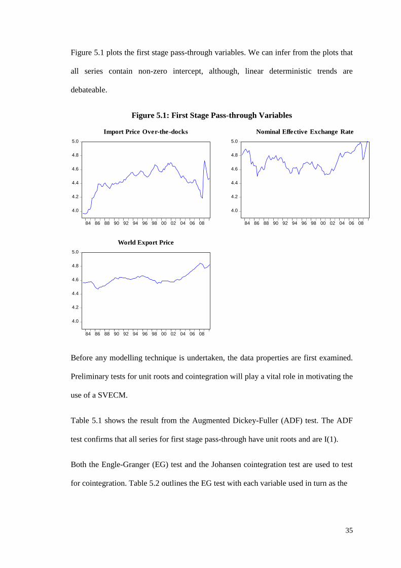
Figure 5.1 plots the first stage pass-through variables. We can infer from the plots that

all series contain non-zero intercept, although, linear deterministic trends are

debateable.

Figure 5.1: First Stage Pass-through Variables

Before any modelling technique is undertaken, the data properties are first examined.

Preliminary tests for unit roots and cointegration will play a vital role in motivating the

use of a SVECM.

Table 5.1 shows the result from the Augmented Dickey-Fuller (ADF) test. The ADF

test confirms that all series for first stage pass-through have unit roots and are I(1).

Both the Engle-Granger (EG) test and the Johansen cointegration test are used to test

for cointegration. Table 5.2 outlines the EG test with each variable used in turn as the

4.0

4.2

4.4

4.6

4.8

5.0

84 86 88 90 92 94 96 98 00 02 04 06 08

Import Price Over-the-docks

4.0

4.2

4.4

4.6

4.8

5.0

84 86 88 90 92 94 96 98 00 02 04 06 08

Nominal Effective Exchange Rate

4.0

4.2

4.4

4.6

4.8

5.0

84 86 88 90 92 94 96 98 00 02 04 06 08

World Export Price

36

Table 5.1: First Stage Augmented Dickey-Fuller Test Results

Variables

Level First Differences

Lags

Test

Stats

CV at

5%

P-

value

Lags

Test

Stats

CV at

5%

P-

value

D

tp 6 -2.72 -3.45 0.23 5 -5.01 -2.89 0.00

te 11 -2.23 -2.89 0.20 11 -3.77 -2.89 0.00

W

tp 6 -1.77 -3.45 0.71 0 -5.59 -2.89 0.00

Lag length selected based on t-statistics with maximum lag length of 12.

Constant and linear trend only included in the levels of import price and world price.

P-value is based on MacKinnon (1996) one sided P-value.

Table 5.2: First Stage Pass-through Engle-Granger Test Results

Dependent Variable Lags t-statistics P-value

D

tp 0 -3.77 0.06

te 0 -4.01 0.03 W

tp 0 -2.43 0.53

Selection of lags based on t-statistics with 5 maximum included lags.

Null hypothesis: No cointegration

Table 5.3: First Stage Pass-through Johansen Cointegration Test Results

Level VAR (3)

Trace Maximum Eigenvalue

Rank

Test

statistics 5% CV P-value

Test


0 37.59* 35.19 0.03 23.76* 22.30 0.03

1 13.83 20.26 0.30 10.53 15.89 0.29

2 3.3 9.16 0.53 3.30 9.16 0.53

*Statistically significant at 5% level. Intercept in CE with no deterministic trend included in both CE and VAR.

Table 5.4: First Stage Pass-through Estimation Results

Variables

Normalised CI

Coefficients

OLS DOLS

Coefficients

Coefficients P-value

te -0.93

(0.18) -1.21

-1.18

(0.22) 0.00

W

tp 0.72

(0.25) 0.72

0.70

(0.15) 0.00

Constant is included in regression but omitted from report.

DOLS using AIC (Max lag length 5) lag and lead both equal to three with HAC standard errors (fixed

4 lags).

Standard errors reported in parenthesis.

The reported long-run elasticity are in the form of 1 1 1 2 1

D W

t t tp e p .

37

dependent variable. We conclude from the result that cointegration is present for the

first stage pass-through.

Before the implementation of the Johansen procedure, the number of lags included in

the test is guided by a set of information criterions from the estimation of the levels

VAR for each pass-through stage. The residuals of the selected model are checked for

serial correlation5.

The Johansen cointegration test results are shown in Table 5.3. We can infer one

cointegrating relationship exists amongst the first stage pass-through variables from

both the trace and maximum eigenvalue test statistics at the 5% level of significance.

The normalised cointegrating coefficients are used to compare with those estimates

obtained from OLS and Dynamic OLS (DOLS) regressions6. Results from Table 5.4

suggest the long-run elasticity of exchange rate is approximately 0.93, which is close

to the theoretical complete pass-through. This is broadly consistent to the coefficients

on exchange rates for both OLS and DOLS, although these estimates suggest slightly

higher than 100% pass-through on the exchange rate.

5.2 Model Estimation and Identification

The Johansen cointegration test indicates the presence of one cointegrating

relationship. However, in order to determine which variables are attribute to the

transitory shock and permanent shocks, estimation of reduced-form VECM(2) is

drawn7. From the model estimation presented in Table 5.5, the results show the

adjustment coefficients on the error correction term for the growth in world price is

5 Please refer to Appendix 2 for details on VAR lag length selection.

6 The coefficient on import price variable,

, is normalised to one in order to determine the long-run

elasticity of the exchange rate and the world price. 7 VECM(2) is constructed using 2 lags of differenced endogenous variables with an intercept in the

cointegrating vector, but no other deterministic components.

38

statistically insignificant at a 5% level. Additionally, both import price and exchange

rate show statistically significant results at a 5% level, however, exchange rate shows

insignificant result at a 1% level. According to the most significant adjustment

coefficient on import price, we infer that the transitory shock is derived from import

price and the two permanent shocks are derived from world price and exchange rate.

Table 5.5: First Stage Adjustment Coefficients Implied By Johansen Normalised

Coefficients on Error Correction of VECM(2)

Dependent

Variable

Independent

Variables Coefficient t-statistics

D

tp 1tec -0.18

(0.04) -4.91*

te 0.13

(0.05) 2.43**

W

tp 0.003

(0.01) 0.33

* Statistically significant at 1%.

** Statistically significant at 5%.

Error correction term is defined as 1 1 1 10.93 0.72 4.96D W

t t t tec p e p using normalised

cointegrating coefficient from the Johansen test presented in Table 5.4.

Application of the identification scheme under weak exogeneity outlined in the

econometrics methodology chapter is now implemented for the first stage. The

structural model for the first stage pass-through is represented as follows:

0,11 0,12 0,13 1 1

0,21 0,22 0,23 1 2 3 1 2

0,31 0,32 0,33 1 3

W

D

W p D

t t t

e

t t t

D Wpt t t

p b b b p

e b b b e

p b b b p

(5.1)

The identifying structural cointegration restrictions can be applied to the first stage

pass-through:

0,11 0,12 0,13

0,21 0,22 0,23

0

0

W

D

p

e

p

b b b

b b b

(5.2)

1tec

1tec

39

The structural systems of equations under the imposed set of identifying cointegrating

restrictions with normalised cointegrating vector can be represented in the following

expanded matrix notation:

0,11 0,12 0,13 1 1

* *

0,21 0,22 0,23 2 3 1 2

0,31 0,32 0,33 1 3

0

0 1D

W D

t t t

t t t

D Wpt t t

p b b b p

e b b b e

p b b b p

(5.3)

where,

0

rB denotes the last row of the impact matrix 0B attributed to the transitory component.

The adjustment coefficient for the world price and the exchange rate is assumed to be

zero with the normalised coefficients for the cointegrating vector. Fisher and Huh

(2012) argued that once zero is imposed on both Wp and e , the coefficients

0,13b

and 0,23b are also zero. This restriction implies that the world price and the exchange

rate do not contemporaneously respond to the structural import price shocks.

Furthermore, a Choleski decomposition can be used to exactly identify the three

variable system if the coefficient 0,12b is restricted to zero. The described restrictions

can be shown through the 0B matrix8:

1 1

* *

2 3 1 2

1 3

1 0 0 0

1 0 0 1

1 D

W D

t t t

t t t

D Wpt t t

p p

e e

p p

(5.4)

where, denotes unrestricted coefficient on the impact multiplier matrix.

8 The main diagonal is normalised to unity for construction of one standard deviation shock.

40

5.3 Main Results for First Stage Pass-through

The impulse response functions generated from the imposed Johansen normalised

coefficients with Choleski ordering are presented in Figure 5.2. This shows the

impulse responses of the world price, the exchange rate, and the import price to a one

standard deviation shock to each of the permanent and transitory shocks9.

In the first panel, the world price responds most to the first permanent shock, while the

second permanent shock and the transitory shock have smaller effects on the world

price.

Figure 5.2: First Stage Impulse Response for One Standard Deviation Permanent

and Transitory Shocks With Johansen Normalised Coefficient: Full Sample

9 PW = World Price, TWI = Exchange Rate, PD = Import Price Over-the-docks.

-.04%

-.02%

.00%

.02%

.04%

.06%

2 4 6 8 10 12 14 16 18 20 22 24

P1 (PW) P2 (TWI) T1 (PD)

1. Response of World Price to

One S.D. Innovations

-.04%

-.02%

.00%

.02%

.04%

.06%

2 4 6 8 10 12 14 16 18 20 22 24


2. Response of Exchange Rate to


-.04%

-.02%

.00%

.02%

.04%

.06%

2 4 6 8 10 12 14 16 18 20 22 24


3. Response of Import Price Over-the-docks

to One S.D. Innovations

41

From the second panel, we see that a permanent shock (attributed to the world price)

has a persistent effect on the exchange rate. There is little response by either the world

price or the exchange rate to the transitory shock, per panel 1 and 2. The transitory

shock does have an initially large impact on the domestic import price shown in the

third panel. However, the effect does not persist in the long-run.

The third panel shows the response of import prices over-the-docks to the three shocks.

Both of the permanent shocks produce a decline in import prices. The second of the

permanent shocks, if interpreted as a positive exchange rate shock (an appreciation), is

associated with a fall in import prices. Hence, the second stage pass-through can be

built on the ground that near to full pass-through does occur in the first stage.

The forecast error variance decomposition is reported in Table 5.6. Firstly, 98% of the

forecast error variance for the world price can be attributed to the first permanent

shock. This pattern is maintained throughout the forecasted horizon. The remaining 2%

is attributed to the second permanent shock and the transitory shock. Secondly, in the

initial forecast horizon, most of the error variance of exchange rate is attributed to the

second permanent shock. However, as the forecast horizon rises, the importance of this

shock decreases and that of the first permanent shock increases. Lastly, as the forecast

horizon rises, more of the variance in the import price is due to the permanent shocks

than the transitory shock.

42

Table 5.6: First Stage Variance Decomposition of Permanent and Transitory

Shocks for Full Sample Period

Percentage of the variance in forecast error of W

tp due to:

Quarters

ahead

Permanent shock 1

1

Wp

t

Permanent shock 2

2

e

t

Transitory shock

3

Dp

t

1 100 0.00 0.00

2 98.55 1.30 0.14

3 98.00 1.90 0.10

4 98.22 1.85 0.06

8 98.26 1.72 0.02

12 98.29 1.70 0.01

16 98.31 1.68 0.01

20 98.32 1.68 0.01

Percentage of the variance in forecast error of te due to:

Quarters

ahead

Permanent shock 1

1

Wp

t

Permanent shock 2

2

e

t

Transitory shock

3

Dp

t

1 6.25 93.75 0.00

2 8.87 91.05 0.08

3 13.61 85.32 1.07

4 17.37 81.32 1.31

8 24.38 74.77 0.84

12 28.93 70.47 0.59

16 31.99 67.56 0.45

20 34.14 65.50 0.35

Percentage of the variance in forecast error of D

tp due to:

Quarters

ahead

Permanent shock 1

1

Wp

t

Permanent shock 2

2

e

t

Transitory shock

3

Dp

t

1 4.34 14.94 80.73

2 8.12 41.69 50.19

3 18.45 43.49 38.06

4 28.70 40.67 30.63

8 37.91 43.73 18.36

12 37.62 48.74 13.64

16 35.43 53.52 11.05

20 33.07 57.57 9.36

43

5.4 Australian Inflation Targeting Subsample

The results from the last section show the quick adjustment of the import price in

response to a highly persistent permanent shock to the exchange rate utilising the full

sample. However, the apparent high pass-through could be triggered by changes in

certain major policies. One of the major policy changes was the announcement of

inflation targeting by the RBA in mid 1993 with the intention to constrain inflation to

2-3% in the medium term. This implies that the central bank will actively utilise

monetary policy to combat medium term inflation. Thus, the stabilisation of the

exchange rate in response to a monetary policy shock would be affected, and hence,

Figure 5.3: First Stage Impulse Response for One Standard Deviation Permanent

and Transitory Shocks With DOLS Estimates: 1983Q2 - 1993Q1

-.04%

-.02%

.00%

.02%

.04%

.06%

2 4 6 8 10 12 14 16 18 20 22 24




-.04%

-.02%

.00%

.02%

.04%

.06%

2 4 6 8 10 12 14 16 18 20 22 24




-.04%

-.02%

.00%

.02%

.04%

.06%

2 4 6 8 10 12 14 16 18 20 22 24




44

pass-through to import price. Thus, two subsample tests involve the periods 1983Q2 to

1993Q1 just prior to the announcement of inflation targeting and post inflation

targeting period of 1993Q2 to 2010Q1.

Figure 5.3 presents the impulse response functions generated from the implied DOLS

estimates used for the cointegration equation in the periods of 1983Q2-1993Q110

.

From the third panel, the response of import price to a one standard deviation increase

in second permanent shock is approximately consistent when compared to the main

results reported. The shock persists with a long-run equilibrium of approximately

0.031%. The speed of adjustment is quick, thus consistent with the main result, where

import price reached its long-run equilibrium level after one year. Interestingly, the

import price reacts less in magnitude to the first permanent shock than in the main

results and the response of the import price levels off to zero in the long-run.

The impulse response functions shown in Figure 5.4 is generated from estimated

DOLS coefficients from the 1982Q2 to 1993Q1 subsample. This is due to the incorrect

sign on the world price shown in Table A5.3 in Appendix 5 for all three methods. In

the third panel, the magnitude of the response of the import price to the second

permanent shock is consistent with the results from subsample prior inflation targeting.

However, the speed of pass-through is much slower than the prior inflation targeting

subsample. Thus, we can draw from the two subsamples that inflation targeting

reduces the speed of exchange rate pass-through to import price, although the

magnitude is broadly consistent across the long-run forecast horizon.

10

Implied DOLS estimates are used instead of the Johansen normalised coefficients due to the two pass-

through coefficients been above 1. Both sets of estimates are reported in Appendix 5 (Table A5.1).

45

From the forecast error variance decomposition in Table 5.7, the same conclusion can

be drawn compared to the corresponding forecast error variance in Table 5.6. The

importance of the second permanent shock increased substantially, which is reflected

Figure 5.4: First Stage Impulse Responses for One Standard Deviation

Permanent and Transitory Shocks With DOLS Estimates: 1993Q2 - 2010Q1

in the first period, where half of the variance in import price is attributed to the second

permanent shock. There seems to be a high and persistent pass-through of the

exchange rate to the import price prior to inflation targeting. Overall, the pass-through

of a permanent shock derived from innovations of the exchange rate to the import

price is complete and significant.

-.06%

-.04%

-.02%

.00%

.02%

.04%

.06%

2 4 6 8 10 12 14 16 18 20 22 24




-.06%

-.04%

-.02%

.00%

.02%

.04%

.06%

2 4 6 8 10 12 14 16 18 20 22 24




-.06%

-.04%

-.02%

.00%

.02%

.04%

.06%

2 4 6 8 10 12 14 16 18 20 22 24




46


Shocks for Subsample 1983Q2-1993Q1


tp due to:

Quarters

ahead

Permanent shock 1

1

Wp

t

Permanent shock 2

2

e

t

Transitory shock

3

Dp

t

1 100 0.00 0.00

2 99.25 0.67 0.08

3 98.30 1.66 0.04

4 97.10 2.86 0.04

8 95.37 4.58 0.05

12 94.61 5.34 0.05

16 94.19 5.77 0.04

20 93.93 6.04 0.03


Quarters

ahead

Permanent shock 1

1

Wp

t

Permanent shock 2

2

e

t

Transitory shock

3

Dp

t

1 4.34 95.66 0.00

2 8.11 91.89 0.00

3 16.98 82.78 0.24

4 20.76 79.04 0.20

8 30.12 69.68 0.19

12 33.03 66.80 0.17

16 33.88 65.98 0.14

20 34.03 65.86 0.11


tp due to:

Quarters

ahead

Permanent shock 1

1

Wp

t

Permanent shock 2

2

e

t

Transitory shock

3

Dp

t

1 1.35 50.81 47.84

2 0.40 82.06 17.55

3 5.37 77.39 17.24

4 10.35 74.33 15.32

8 15.60 75.09 9.31

12 14.30 78.75 6.95

16 11.93 82.50 5.56

20 9.88 85.49 4.62

47


Shocks for Subsample 1993Q2-2010Q1


tp due to:

Quarters

ahead

Permanent shock 1

1

Wp

t

Permanent shock 2

2

e

t

Transitory shock

3

Dp

t

1 100 0.00 0.00

2 97.31 2.39 0.30

3 96.84 3.01 0.16

4 97.27 2.59 0.14

8 98.21 1.72 0.07

12 98.44 1.51 0.05

16 98.54 1.42 0.04

20 98.60 1.37 0.03


Quarters

ahead

Permanent shock 1

1

Wp

t

Permanent shock 2

2

e

t

Transitory shock

3

Dp

t

1 6.28 93.72 0.00

2 7.40 92.50 0.10

3 9.35 88.55 2.09

4 10.57 86.53 2.90

8 12.12 85.85 2.03

12 15.76 82.73 1.51

16 19.60 79.25 1.15

20 22.97 76.12 0.91


tp due to:

Quarters

ahead

Permanent shock 1

1

Wp

t

Permanent shock 2

2

e

t

Transitory shock

3

Dp

t

1 3.56 15.10 81.34

2 10.18 46.64 43.18

3 23.24 48.87 27.89

4 33.33 45.21 21.46

8 40.33 45.45 14.22

12 38.82 49.72 11.46

16 35.46 54.61 9.93

20 32.06 59.07 8.87

48

Lastly, from the forecast error decompositions presented in Table 5.8, compared to the

previous subsample, the importance of the second permanent shock is diminished to

the variance of import price, while the transitory shock becomes more dominant in the

initial forecast horizons. Thus, inflation targeting contributes to the increased

resilience of the exchange rate pass-through, even in the first stage.

5.5 Rolling Window for Coefficient Stability

To perform a stability check on the long-run coefficients implied by the Johansen

normalised coefficients and DOLS, recursive estimation of Johansen and DOLS

methodology with a window of 20 on the full sample period from 1983Q2 to 2010Q1

is implemented. Figure 5.5 reports the recursive rolling window on DOLS estimation

for the first stage pass-through coefficients of the exchange rate and the world price11

.

Figure 5.5: First Stage Pass-through Rolling Window on DOLS Coefficients

From Figure 5.5, the coefficients on both the exchange rate and the world price appear

to be stable with fluctuations between 1.08 to 1.28 for the exchange rate and 0.6 to 1.5

for the world price. Additionally, the 2 standard error bands appear larger with

increasing sample periods, which reflect increased uncertainty in periods after 1993.

11

Rolling window estimates using the Johansen methodology are reported in Appendix 7.

-1.5

-1.4

-1.3

-1.2

-1.1

-1.0

-0.9

-0.8

88 90 92 94 96 98 00 02 04 06 08

TWI TWI LB TWI UB

0.0

0.4

0.8

1.2

1.6

2.0

88 90 92 94 96 98 00 02 04 06 08

PW PW LB PW UB

49

6. Second Stage Pass-through: Import Price to Inflation

This chapter describes how much of the first stage exchange rate fluctuations pass-

through from the after-tax import prices to the domestic retail price. Thus, the

dynamics of the import price to inflation will be assessed. I will address the role

played by the mark-up on cost to help explain the adjustment of prices to fluctuations

in the exchange rate. The chapter concludes with the inflation targeting subsample

used to determine whether the announcement of inflation targeting triggers any

differences in variations of mark-up on cost. In addition, stability tests are conducted

on the long-run coefficients.

6.1 Data Description and Properties

Second stage pass-through variables include: the retail price of consumption goods

( )D

tr , the after-tax import price over-the-docks ( )T

tp , and the costs borne by retailers

and importers ( )C

tp . All data obtained are in quarterly frequency with the same sample

periods consistent with the first stage analysis.

The retail price imported consumption goods is constructed using five consumption

subgroups or expenditure classes sourced from the ABS all group CPI. This proxy

entails the need to re-weight each subgroup or expenditure class by their respective

historical weights. These weights are also sourced from the ABS. Thus, all five

weighted subgroups or expenditure classes are aggregated to form a proxy for the

retail price of consumption goods.

In comparison to the approach used by Dwyer and Lam (1994), they deducted

weighted sub-groups or expenditure classes from the total CPI that were not

predominately imported consumption goods. The rest were aggregated to form a proxy

50

for retail price of consumption. This approach is not followed due to several issues that

arose with the sampled data. The main issue is due to missing observations in earlier

quarters and re-categorisation of subgroups or expenditure classes of the sample data1.

The after-tax import price is simply the tariff-adjusted import price over-the-docks

from the first stage. This series is defined as import price times the index of (1 +

average tariff). Average tariff is defined as taxes on international trade in proportion to

the value of merchandise imports, consistent with Dwyer and Lam (1994).

Five major costs are distinguished, namely: international freight cost, taxes on

international trade, unit labour costs, domestic transport cost, and other expenses.

However, the series excludes the tax on international trade due to its inclusion in after-

Figure 6.1: Second Stage Pass-through Variables

1 Please refer to Appendix 1 for a full treatment of data issues.

3.8

4.0

4.2

4.4

4.6

4.8

5.0

84 86 88 90 92 94 96 98 00 02 04 06 08

Retail Price of Consumption Goods

3.8

4.0

4.2

4.4

4.6

4.8

5.0

84 86 88 90 92 94 96 98 00 02 04 06 08

After-tax Import Price

3.8

4.0

4.2

4.4

4.6

4.8

5.0

84 86 88 90 92 94 96 98 00 02 04 06 08

Input Costs Borne by Retailers and Importers

51

tax import price. All series are obtained from the ABS website with the exception of

domestic freight. Domestic freight is sourced from the Australian Bureau of

Agricultural and Resource Economics (ABARE). However, the data sample ends in

Q1 2010. The construction of these costs is consistent to that of Dwyer and Lam (1994)

with only minor change to other expenses.

Figure 6.1 shows graphical representations of the second stage pass-through variables.

We can infer from the plots that all series contains non-zero intercept with linear trend,

although, linear trend in import price is debateable.

The ADF test presented in Table 6.1 shows all variables contain a unit root and their

levels are I(1)2. The EG test presented in Table 6.2 shows no cointegration amongst

any group of variables. However, from the Johansen test presented in Table 6.3, the

trace statistics show one cointegration relationship amongst the variables, while the

maximum eigenvalue statistics shows no cointegration relationship at 5% level.

Although, only trace statistics show one cointegration relationship, the specification of

including the deterministic trend is to be used as a sensitivity check for robustness of

the main result in second stage pass-through3.

The normalised cointegrating coefficient shown in Table 6.4 suggests the long-run

elasticity between retail price and after-tax import price is positive with a magnitude of

above 3. In comparison to Dwyer and Lam (1994), their long-run elasticity of 0.66 is

much lower than the estimate obtained from the Johansen methodology. The OLS and

DOLS estimate for import price is relatively similar to the estimated coefficients in

2 Although, retail price seems to be marginally I(1) shown in the ADF test, however, theory suggest that

retail price is I(1), thus, retail price is treated as I(1). 3 Impulse response functions are generated for both first and second stage pass-through with the

inclusion of trend specifications reported in Appendix 6.

52

Table 6.1: Second Stage Augmented Dickey-Fuller Test Results

Variables

Level First Differences

Lags Test

Stats

CV at

5%

P-

value Lags

Test

Stats

CV at

5%

P-

value

D

tr 2 -3.28 -3.45 0.07 1 -2.40 -2.89 0.14

T

tp 6 -2.94 -3.45 0.15 1 -8.61 -2.89 0.00

C

tp 0 -2.58 -3.45 0.29 0 -11.05 -2.89 0.00

Lag length selected based on t-statistics with maximum lag length of 12.

Constant and linear trend included in the levels of all three variables.

P-value is based on MacKinnon (1996) one sided P-value.

Table 6.2: Second Stage Pass-through Engle-Granger Test Results

Dependent Variable Lags t-statistics P-value D

tr 4 -2.34 0.57 T

tp 4 -2.37 0.56 C

tp 4 -1.98 0.74



Table 6.3: Second Stage Pass-through Johansen Cointegration Test Results

Level VAR (3)

Trace

Maximum Eigenvalue

Rank

Test


Test


0 41.29* 35.19 0.01 21.76 22.30 0.06

1 19.53 20.26 0.06 12.97 15.89 0.14

2 6.56 9.16 0.15 6.56 9.16 0.15

*Statistically significant at 5% level.

Intercept in CE with no deterministic trend included in both CE and VAR4.

Table 6.4: Second Stage Pass-through Estimation Results

Variables

Normalised CI

Coefficients

OLS DOLS

Coefficients


Tp 3.05

(0.82) 0.44

0.43

(0.15) 0.01

Cp 2.43

(0.73) 0.75

0.71

(0.04) 0.00

Constant included in regression but omitted from report.


4 lags).


The reported normalised coefficients are in the form of 1 1 1 2 1

D T C

t t tr p p .

4 Deterministic trend is excluded from estimation results since it is statistically insignificant at 5% level.

53

Dwyer and Lam (1994). The DOLS estimates are used to form the error correction

term in the following sections.


From Table 6.5, the estimation results from a VECM(2) specification shows the

adjustment coefficients on the error correction term is statistically insignificant at the 5%

level for both growth in retail price and after-tax import price5. However, the growth

Table 6.5: Adjustment Coefficients on Error Correction of VECM(2)

Dependent

Variable

Independent


D

tr 1tec -0.01

(0.01) -1.21

T

tp 0.12

(0.10) 1.15

C

tp 0.17

(0.05) 3.51**

* Statistically significant at 5%

** Statistically significant at 1%

Error correction term is defined as 1 1 1 10.43 0.71 0.59D T C

t t t tec r p p using DOLS estimated

coefficients from Table 6.4.

of total costs inputs shows a statistically significant result even at 1%. Hence, given

the current specifications, we can draw from the result that the transitory shock is

derived from the input costs and the two permanent shocks derives from the retail

price and the import price.

The identification strategy under weak exogeneity seen in the first stage is also

implemented for the second stage. Identifying structural cointegrating restrictions

analogous to the first stage involve the following:

5 VECM(2) is constructed using 2 lags of differenced endogenous variables with intercept but no trend

in cointegrating vector.

1tec

1tec

54

0,11 0,12 0,13

0,21 0,22 0,23

0

0

T

D

C

p

r

p

b b b

b b b

(6.1)

Consequently, the result of the structural system under the imposed identifying

structural restrictions with the equivalent Choleski decomposition for the second stage

becomes:

1 1

* *

2 3 1 2

1 3

1 0 0 0

1 0 0 1

1 C

T D

t t t

D T

t t t

C Cpt t t

p r

r p

p p

(6.2)

6.3 Main Results for Second Stage Pass-through

Figure 6.2 presents the response of each of the variables to a one standard deviation

increase in each of the permanent and transitory shocks6. The second panel shows two

important results. Firstly, a one standard deviation permanent shock thought to be

attributed to import price increased retail price by 0.018% in the long-run equilibrium.

Specifically, compared to the first stage pass-through, the speed of pass-through is

very slow; by the end of one year, only 0.002% of the first shock is transmitted to the

domestic retail price. Additionally, the magnitude over the long-run equilibrium is

approximately 0.018%, which is almost half as low as 0.033% for the long-run pass-

through of the exchange rate to import price in the first stage.

Secondly, the role of the mark-up in retail prices can be seen from the transitory shock,

as it appears that there is no impact of a raise in mark-up on the retail price7.

6 PT = After-tax Import Price, RPI = Retail Price of Imported Consumption Goods, PC = Input Costs

Borne By Retailers and Importers. 7 The cause of the result is due to the assumption that both after-tax import price and retail price does

not adjust contemporaneously with input cost. As a robustness check, zero restrictions will be imposed

on the adjustment coefficients for import price and input costs to compare with the main results.

55

Furthermore, the role of mark-up in relation to import price can also be drawn from

the first panel. The response of the after-tax import price declined after the transitory

Figure 6.2: Impulse Responses for One Standard Deviation Permanent and

Transitory Shocks With DOLS Estimates: Full Sample

shock attributed to the mark-up. However, due to the nature of transitory shock, the

response of import price drives back to zero long-run equilibrium. By combining this

result with previous findings, an unfavourable shock in exchange rate raises import

price, thus lowers mark-up (shown in panel 1), and increases the retail price (shown in

panel 2)8.

8 Consequently, a favourable exchange rate shock reduces the import price due to retailers response of

reducing their mark-up on costs and reduces retail price.

-.04%

-.02%

.00%

.02%

.04%

.06%

.08%

10 20 30 40 50 60 70 80 90 100

P1 (PT) P2 (RPI) T1 (PC)

1. Response of After-tax Import Price to


-.04%

-.02%

.00%

.02%

.04%

.06%

.08%

10 20 30 40 50 60 70 80 90 100


2. Response of Retail Price to


-.04%

-.02%

.00%

.02%

.04%

.06%

.08%

10 20 30 40 50 60 70 80 90 100


3. Response of Input Costs to


56

One final result can be drawn from the last panel that a one standard deviation

permanent shock attributed to the retail price raises the domestic input costs in the

long-run. The magnitude is large and significant. In addition, the first permanent shock

reduces the total input costs. This means that domestic shock has an important

influence on the input cost decisions faced by domestic retailers.

From the forecast error variance decomposition shown in Table 6.6, initially, most of

the error variance in growth of retail price is attributed to the second permanent shock.

However, the first permanent shock attributed to the after-tax import price slowly

increased confirming the speed of pass-through is slow. Interestingly, the last section

in Table 6.6 shows the increasing role of the first permanent shock quickly dominated

the forecast error variance of growth in input costs after one year period. This is

consistent with the claim made before that domestic import price shock has an

important role in input costs decisions faced by retailers.

57

Table 6.6: Variance Decomposition of Permanent and Transitory Shocks: Full

Sample Period

Percentage of the variance in forecast error of T

tp due to:

Quarters

ahead

Permanent shock 1

1

Tp

t

Permanent shock 2

2

Dr

t

Transitory shock

3

Cp

t

1 100 0.00 0.00

2 99.17 0.51 0.32

3 97.50 1.25 1.26

4 96.26 1.99 1.75

8 94.65 3.86 1.49

12 93.39 5.42 1.20

16 92.49 6.55 0.96

20 91.89 7.33 0.78


tr due to:

Quarters

ahead

Permanent shock 1

1

Tp

t

Permanent shock 2

2

Dr

t

Transitory shock

3

Cp

t

1 1.17 98.83 0.00

2 0.49 99.50 0.01

3 1.10 98.89 0.00

4 1.88 98.10 0.01

8 3.30 96.63 0.07

12 4.22 95.70 0.08

16 4.90 95.03 0.08

20 5.45 94.48 0.07

Percentage of the variance in forecast error of C

tp due to:

Quarters

ahead

Permanent shock 1

1

Tp

t

Permanent shock 2

2

Dr

t

Transitory shock

3

Cp

t

1 2.60 2.08 95.31

2 2.19 1.62 96.19

3 4.87 1.22 93.91

4 7.36 1.18 91.45

8 21.21 7.03 71.77

12 32.80 19.17 48.02

16 37.45 31.70 30.85

20 37.66 42.09 20.25

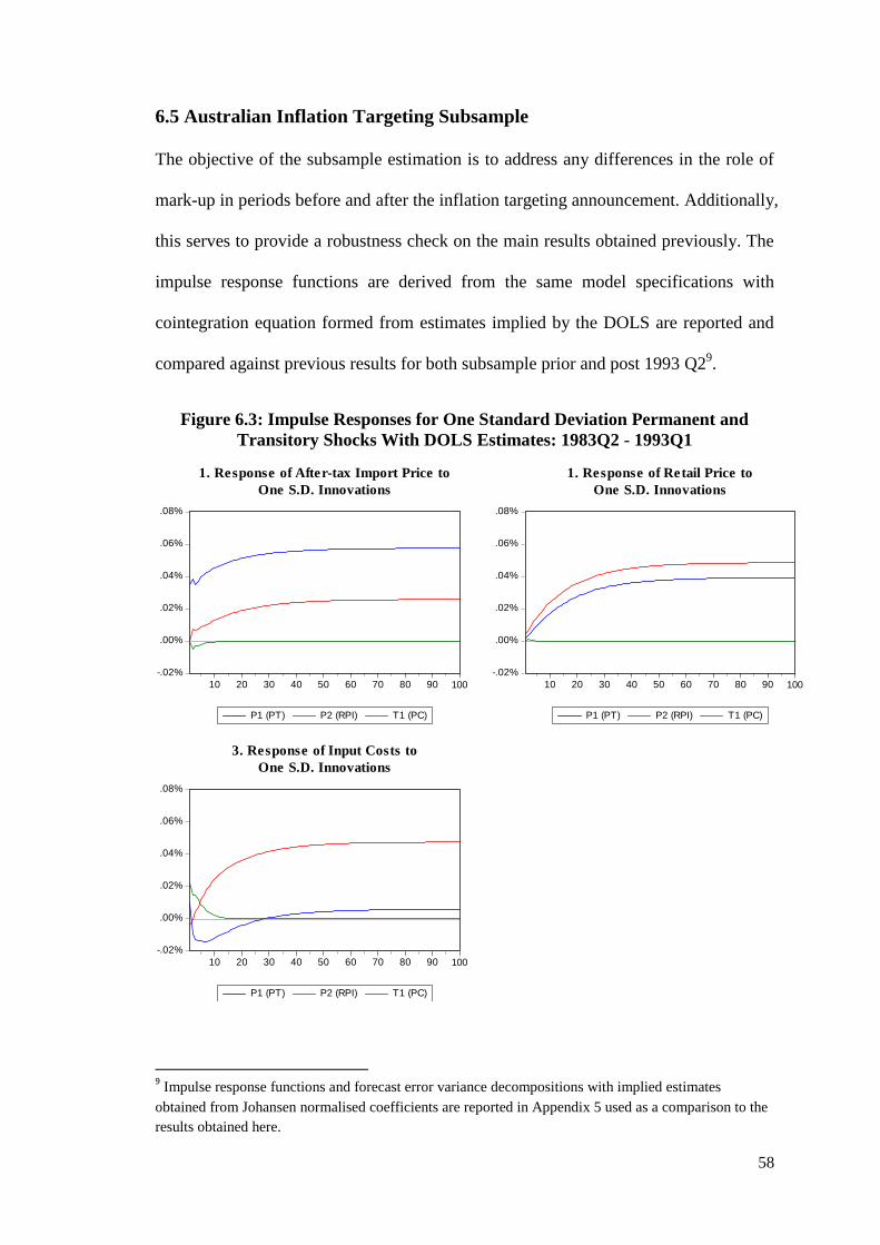
58

6.5 Australian Inflation Targeting Subsample

The objective of the subsample estimation is to address any differences in the role of

mark-up in periods before and after the inflation targeting announcement. Additionally,

this serves to provide a robustness check on the main results obtained previously. The

impulse response functions are derived from the same model specifications with

cointegration equation formed from estimates implied by the DOLS are reported and

compared against previous results for both subsample prior and post 1993 Q29.


Transitory Shocks With DOLS Estimates: 1983Q2 - 1993Q1

9 Impulse response functions and forecast error variance decompositions with implied estimates

obtained from Johansen normalised coefficients are reported in Appendix 5 used as a comparison to the

results obtained here.

-.02%

.00%

.02%

.04%

.06%

.08%

10 20 30 40 50 60 70 80 90 100




-.02%

.00%

.02%

.04%

.06%

.08%

10 20 30 40 50 60 70 80 90 100




-.02%

.00%

.02%

.04%

.06%

.08%

10 20 30 40 50 60 70 80 90 100




59

Figure 6.3 shows the impulse response functions generated using the implied

estimated cointegrating coefficients from the DOLS regression. The second panel

shows the long-run equilibrium of a one standard deviation permanent shock attributed

to import price raises the response of retail price by approximately 0.04%. Compared

to the previous second panel in the main result, the magnitude is twice as large and the

speed of pass-through is slightly faster. The role of the mark-up in the first panel is

slightly diminished compared to the main results. However, since input costs generate

transitory shock, retail price is still unaffected by change in the mark-up. Additionally,

the response of all included variables are persistent to the second permanent shock

derived from retail price. Overall, the impulse response functions are robust to the

main results obtained previously.

Figure 6.4 shows impulse response functions during post inflation targeting

announcement derived from the implied DOLS estimates10

. Compared to Figure 6.3,

with the exact same specification using imposed DOLS estimates for periods prior to

inflation targeting, and the pass-through here is negligible in magnitude with

approximately the same speed. The only difference is due to the change in the

persistence of the shock; input cost is attributed to transitory shock prior inflation

targeting, while retail price becomes transitory post inflation targeting. Thus, we can

draw from the two subsamples that the effect of inflation targeting caused the decline

in persistency of shock that attributed to retail price and raised the persistency of input

costs.

Furthermore, the third panel shows that the transitory shock attributed to the mark-up

raises the long-run equilibrium of retail price by approximately 0.012%. Comparing to

10

Implied DOLS estimates were used to substitute the Johansen normalised coefficients since the

coefficient on import price had incorrect sign.

60

the previous prior inflation target sample, the role of mark-up becomes important after

the announcement and implementation of inflation targeting by RBA. Thus, the

reduction in persistency of retail price with a more fluctuating and persistent mark-up

on cost implies reduction in pricing power of retailers consistent with Taylor (2000).

In summary, the portion of the permanent shock derived from exchange rate change is

absorbed by variation in mark-up after the implementation of inflation targeting,

although, mark-up plays a limited role prior inflation target periods.


Transitory Shocks With DOLS Estimates: 1993Q2 - 2010Q1

-.02%

.00%

.02%

.04%

.06%

.08%

10 20 30 40 50 60 70 80 90 100

P1 (PT) P2 (PC) T1 (RPI)



-.02%

.00%

.02%

.04%

.06%

.08%

10 20 30 40 50 60 70 80 90 100




-.02%

.00%

.02%

.04%

.06%

.08%

10 20 30 40 50 60 70 80 90 100




61

Table 6.7: Second Stage Variance Decomposition of Permanent and Transitory

Shocks Implied By DOLS Estimates: 1983Q2-1993Q1


tp due to:

Quarters

ahead

Permanent shock 1

1

Tp

t

Permanent shock 2

2

Dr

t

Transitory shock

3

Cp

t

1 100 0.00 0.00

2 97.08 1.95 0.97

3 96.60 2.52 0.87

4 96.30 2.91 0.79

8 95.28 4.31 0.41

12 94.07 5.68 0.25

16 92.86 6.97 0.17

20 91.75 8.12 0.12


tr due to:

Quarters

ahead

Permanent shock 1

1

Tp

t

Permanent shock 2

2

Dr

t

Transitory shock

3

Cp

t

1 8.85 91.15 0.00

2 15.97 82.98 1.05

3 20.59 78.99 0.41

4 24.26 75.51 0.23

8 30.11 69.85 0.04

12 32.87 67.11 0.02

16 34.50 65.49 0.01

20 35.56 64.43 0.01


tp due to:

Quarters

ahead

Permanent shock 1

1

Tp

t

Permanent shock 2

2

Dr

t

Transitory shock

3

Cp

t

1 15.88 2.43 81.69

2 20.74 1.64 77.62

3 27.00 2.40 70.60

4 32.43 4.63 62.94

8 35.95 31.42 32.64

12 27.54 54.57 17.89

16 19.75 69.07 11.18

20 14.29 78.02 7.68

62

In comparison of the forecast error decompositions between two of the subsamples

shown in Table 6.7 and Table 6.8, two results are drawn. The subsample prior to

inflation target shows the first permanent shock (import price) has a higher

contribution to the variance in retail price compared to the full sample. However, the

role of the same shock is much lower in the post inflation targeting announcement

period shown in last section of Table 6.8. Consequently, the role of the mark-up

becomes significant in the variance of retail price post inflation target period.

A further result lies in the differences of the first permanent shock to the variance of

input costs between the two subsamples. After the implementation of inflation

targeting, the first permanent shock plays no role in explaining the input costs. This

implies that the result obtained from the full sample forecast error decompositions is

driven by the significance of the role in import price shock prior to the inflation

targeting.

63

Table 6.8: Second Stage Variance Decomposition of Permanent and Transitory

Shocks Implied By DOLS Estimates: 1993Q2-2010Q1


tp due to:

Quarters

ahead

Permanent shock 1

1

Tp

t

Permanent shock 2

2

Cp

t

Transitory shock

3

Dr

t

1 100 0.00 0.00

2 99.80 0.01 0.19

3 98.70 0.89 0.40

4 97.53 2.03 0.44

8 97.97 1.71 0.33

12 98.32 1.43 0.25

16 98.60 1.20 0.20

20 98.81 1.02 0.17


tp due to:

Quarters

ahead

Permanent shock 1

1

Tp

t

Permanent shock 2

2

Cp

t

Transitory shock

3

Dr

t

1 1.67 98.33 0.00

2 0.89 97.42 1.69

3 0.82 96.09 3.09

4 0.67 95.45 3.88

8 0.48 95.29 4.23

12 0.41 96.29 3.30

16 0.38 97.14 2.47

20 0.37 97.73 1.89


tr due to:

Quarters

ahead

Permanent shock 1

1

Tp

t

Permanent shock 2

2

Cp

t

Transitory shock

3

Dr

t

1 6.18 1.13 92.69

2 3.33 1.93 94.75

3 2.08 1.23 96.69

4 2.16 1.02 96.82

8 2.71 12.88 84.41

12 3.27 38.86 57.86

16 3.31 59.14 37.16

20 3.18 71.94 24.88

64

6.6 Rolling Window for Coefficients Stability

Similar to the rolling window performed on first stage pass-through results, recursive

estimation with window of 20 was implemented on both Johansen and DOLS

methodology. Figure 6.5 shows the coefficient on both after-tax import prices are

stable with fluctuation ranging from 0.48 to 0.70. Coefficients on input costs shows

greater fluctuations in the periods prior to 1990, which stabilises between 0.50 to 0.80.

Figure 6.5: Second Stage Pass-through Rolling Window on DOLS Coefficients

.2

.3

.4

.5

.6

.7

.8

.9

88 90 92 94 96 98 00 02 04 06 08

PT PT LB PT UB

0.2

0.4

0.6

0.8

1.0

1.2

1.4

1.6

88 90 92 94 96 98 00 02 04 06 08

PC PC LB PC UB

65

7. Combined Stage Pass-through: Exchange Rate to Retail Price

The motivation of this chapter is two-fold. The first is to trace out the direct impact of

the exchange rate changes on domestic retail prices. More importantly, the

decomposition of import prices into the exchange rate and the world price allow

further insight on how mark-up varies with the exchange rate additional to the

response of retail price.

7.1 Data Properties

This section shows the evidence towards the removal of the tariff component on the

after-tax import price when the index of average tariff enters the system as a separate

variable, in accordance with the theoretical framework. Table 7.1 shows the estimated

coefficients from OLS, DOLS, and normalised cointegrating coefficients derived from

the Johansen methodology. The estimates from both the OLS and DOLS both show

the index of average tariff is statistically insignificant at the 5% level. Although, the

long-run elasticity implied by Johansen is statistically significant at 5%, however, it is

insignificant at 1% level.

Table 7.1: Combined Stage Pass-through Estimation Results

Variables Normalised CI

Coefficients

OLS DOLS

Coefficients Coefficients P-value

tT 2.79

(1.35)

-1.14

0.03

(0.66) 0.97

te -0.56

(0.09)

-0.56

-0.39

(0.07) 0.00

W

tp 0.55

(0.21)

0.34

0.13

(0.13) 0.32

C

tp -0.62

(0.16)

0.40

0.81

(0.08) 0.00

Constant and deterministic trend included in all three estimates but omitted from report.

DOLS using AIC (Max lag length 5) lag and lead both equal to five with HAC standard errors (fixed 1

lag).


The reported long-run elasticity are in the form of 1 1 2 1 3 1

D T C

t t t tr T p p

66

Table 7.2: Combined Stage Pass-through Four-Variables VECM Engle-Granger

Test Results

Dependent Variable Lags t-statistics P-value D

tr 2 -2.89 0.50

te 0 -4.08 0.07

W

tp 0 -2.02 0.88

C

tp 2 -2.31 0.79



Table 7.3: Combined Stage Pass-through Four-Variables VECM Johansen

Cointegration Test Results

Level VAR (3)

Trace

Maximum Eigenvalue

Rank

Test


Test


0 50.13* 47.86 0.03 28.67* 27.58 0.04

1 21.46 29.80 0.33 13.87 21.13 0.38

2 7.58 15.49 0.51 6.49 14.26 0.55

3 1.09 3.84 0.30 1.09 3.84 0.30

*Statistically significant at 5% level.

Intercept and deterministic trend included VAR, excluded from CE1.

Table 7.4: Combined Stage Pass-through Four-Variables VECM Estimation

Results

Variables Normalised CI

Coefficients

OLS DOLS

Coefficients Coefficients P-value

te -0.56

(0.09)

-0.56

-0.54

(0.08) 0.00

W

tp 0.58

(0.20)

0.29

0.41

(0.12) 0.00

C

tp 0.38

(0.09)

0.54

0.71

(0.05) 0.00


DOLS using AIC (Max lag length 5) lag and lead both equal to three with HAC standard errors

(fixed 1 lag).


The reported long-run elasticity are in the form of 1 1 2 1 3 1

D W C

t t t tr e p p

1 Linear deterministic trend is found to be statistically significant. Hence, trend is included into the

regressions.

67

The exclusion of the index of average tariff reduces a five-variable VECM to a four-

variable VECM with retail price, exchange rate, world price, and input costs. Table 7.2

and 7.3 summarise the Johansen cointegration test and the EG test respectively. The

EG test provides some evidence of cointegration, while the Johansen test confirms

there exists one cointegration relationship amongst the four variables.

Table 7.4 compares the elasticity of long-run estimates obtained from OLS and DOLS

to that of estimates generated from Johansen methodology. From all estimates,

exchange rates are statistically significant with consistent estimates of approximately

0.56. Although, there are some slight differences amongst estimates for world prices

and input costs, nevertheless, all estimates show statistical significance at the 5% level,

except for world price in the DOLS estimates.


From Table 7.5, the results for the VECM (2) model show the adjustment coefficients

for growth in the exchange rate on the error correction term is statistically insignificant

at 5% level2. Additionally, both world price and input costs shows statistically

significant result at 5%, however, both shows insignificant result at 1%. Hence, given

statistical significant result for the growth of retail price, the transitory shock is

derived from the retail price and the three permanent shocks derive from exchange rate,

world price, and input costs.

Despite the significance of the adjustment coefficient on world price and input cost at

5%, but not at 1%, similar to the first stage, we infer that the transitory shock is

derived from the retail price.

2 VECM (2) is constructed using 2 lags of differenced endogenous variables with intercept and trend in

cointegrating vector.

68

Table 7.5: Adjustment Coefficients on Error Correction of VECM(2)

Dependent

Variable

Independent


-0.04

(0.01) -4.29**

0.10

(0.12) -0.85

0.05

(0.02) 2.54*

0.12

(0.05) 2.36*



Error correction term is defined as 1 1 1 1 10.56 0.58 0.38 2.42D W C

t t t t tec r e p p using Johansen

normalised coefficients from Table 7.4.

The identifying structural cointegrating restrictions for the combined stage involve an

extra imposed zero adjustment coefficient shown in the following:

0,11 0,12 0,13 0,14

0,21 0,22 0,23 0,24

0,31 0,32 0,33 0,34

0

0

0

W

C

D

p

e

p

r

b b b b

b b b b

b b b b

(7.1)

Consequently, the result of the structural system under the imposed identifying

restrictions with the equivalent Choleski decomposition for the combined stage

becomes:

11

2* * * 1

2 3 4

31

41

01 0 0 0

01 0 01

01 0

1D

W Dtt t

tt t

C Wtt t

D Crtt t

p r

e e

p p

r p

69

7.3 Main Results for Combined Stage Pass-through

Several key results can be drawn from the impulse response functions in Figure 7.1.

One noticeable difference of all impulse responses compared to the first stage is the

extended amount of time required for the response variables to reach long-run

equilibrium. The first panel shows that the world price responds most to the second

permanent shock believed to be attributed to exchange rate compared to the first

permanent shock. This means that in the long-run, the exchange rate becomes the

dominant factor that drives the world price.

We can also infer from the first panel that, in the long-run, the third permanent shock

attributed to the mark-up on costs will raise the world price by approximately 0.04%.

Thus, domestic mark-up is large and persistent in the long-run, hence, increasingly

influences the world price over the extended forecasted horizon. Conversely, in the

third panel, the first permanent shock (world price) raises the total domestic input cost

by approximately 0.015% in the long-run. Consequently, movements in world price

have some influence on domestic input costs over the long-run. Interestingly, the

fourth panel shows the first permanent shock has a weak influence over the domestic

retail price.

From the second panel, an increase in mark-up on cost shown in the green line

appreciates the exchange rate, while the third panel tells us that a favourable one

standard deviation increase in the second permanent shock attributed to exchange rate

reduces the domestic total costs of inputs. The combination of these two effects

suggest retailers respond to an favourable persistent shock attributed to exchange rate

movement will respond by upward adjustment of mark-up in the face of reduction in

total domestic input costs. Panel 2 and 3 confirm the result from Dwyer and Lam

70

(1994), where retailers perceive total costs to have permanent effect. Furthermore, the

fourth panel shows the long-run equilibrium to a one standard deviation in the third

permanent shock attributed to the mark-up raised retail price by just under 0.04%.

However, the speed of adjustment to long-run equilibrium is shown to be much slower

and gradual over the extended forecast horizon.


Transitory Shocks With Johansen Normalised Coefficients: Full Sample

Another result that can be drawn from the impulse responses is how retail prices vary

with exchange rate movements. The last panel shows a one standard deviation change

in the second permanent shock reduces the retail price by approximately 0.10% in the

long-run. However, the speed of pass-through is very slow; after one year, only 0.005%

reduction in retail price materialises and approximately 0.5% pass-through after 10

-.12%

-.08%

-.04%

.00%

.04%

.08%

50 100 150 200 250 300

P1 (WP) P2 (TWI)

P3 (PC) T1 (RPI)



-.12%

-.08%

-.04%

.00%

.04%

.08%

50 100 150 200 250 300

P1 (WP) P2 (TWI)

P3 (PC) T1 (RPI)



-.12%

-.08%

-.04%

.00%

.04%

.08%

50 100 150 200 250 300

P1 (WP) P2 (TWI)

P3 (PC) T1 (RPI)



-.12%

-.08%

-.04%

.00%

.04%

.08%

50 100 150 200 250 300

P1 (WP) P2 (TWI)

P3 (PC) T1 (RPI)



71

years in forecast horizon. Although, the speed of adjustment is slow, the magnitude of

change is large and gradually increasing up to approximately 200 forecast periods,

before it stabilises.

Overall, we can draw three main conclusions from the four panels. Firstly, a

favourable permanent shock attributed to exchange rate affects the domestic retail

price slowly and large in magnitude as forecast horizon rises. This magnitude reaches

equilibrium at approximately 0.10% in the long-run. Secondly, retailers raise their

mark-up in response to favourable exchange rate movements in the face of a decline in

import price. Lastly, variation in mark-up is slow in response to exchange rate

movements and this persists to effect retail price at approximately 0.04% in the long-

run.

Table 7.6 shows the forecast error decompositions. Most of the forecast error variance

is associated with the first permanent shock, although, the importance of the exchange

rate increases after about two years. This confirms the impulse response functions

where exchange rate plays a dominant role in world price in the later forecast horizons.

Similarly, the first permanent shock becomes increasingly dominant in the variance of

exchange rate as forecast horizon rises. Furthermore, the second permanent shock

becomes increasingly dominant in the error variance in input costs, which support the

role played by mark-up on cost in face of a change in the exchange rate. Lastly, the

importance of the second permanent shock is highlighted in the last section in Table

7.6. Specifically, it demonstrates that after one year, 26% of the error variance of retail

price is explained by the second permanent shock, compared to 41% of the error

variance of import price in the first stage.

72

Table 7.6: Combined Stage Variance Decomposition of Permanent and

Transitory Shocks: Full Sample Period


tp due to:

Quarters

ahead

Permanent

shock 1 1

Wp

t

Permanent

shock 2 2

e

t

Permanent

shock 3 3

Cp

t

Transitory

shock 4

Dr

t

1 100 0.00 0.00 0.00

2 94.31 0.57 1.43 3.69

3 89.60 0.33 5.25 4.82

4 85.97 0.38 7.10 6.55

8 76.04 4.01 10.12 9.84

12 66.06 12.52 12.10 9.32

16 56.40 22.15 13.62 7.82

20 48.02 31.01 14.65 6.32


Quarters

ahead

Permanent

shock 1 1

Wp

t

Permanent

shock 2 2

e

t

Permanent

shock 3 3

Cp

t

Transitory

shock 4

Dr

t

1 4.08 95.92 0.00 0.00

2 5.60 93.53 0.11 0.76

3 6.84 91.90 0.61 0.66

4 7.48 91.01 0.86 0.66

8 9.04 88.70 1.53 0.73

12 10.29 86.73 2.19 0.79

16 11.45 84.79 2.94 0.82

20 12.58 82.79 3.78 0.84


tp due to:

Quarters

ahead

Permanent

shock 1 1

Wp

t

Permanent

shock 2 2

e

t

Permanent

shock 3 3

Cp

t

Transitory

shock 4

Dr

t

1 3.06 1.34 95.59 0.00

2 1.95 2.86 94.55 0.64

3 1.91 2.02 93.42 2.65

4 2.09 1.67 91.38 4.86

8 2.69 7.09 82.42 7.80

12 2.95 15.54 74.14 7.38

16 2.95 24.11 66.74 6.19

20 2.86 31.63 60.48 5.03


tr due to:

Quarters

ahead

Permanent

shock 1 1

Wp

t

Permanent

shock 2 2

e

t

Permanent

shock 3 3

Cp

t

Transitory

shock 4

Dr

t

1 1.09 1.53 1.02 96.36

2 3.76 5.10 0.77 90.37

3 4.17 16.68 0.76 78.38

4 4.96 26.18 0.45 68.40

8 5.35 53.60 1.04 40.00

12 4.65 68.37 2.82 24.17

16 3.96 76.11 4.41 15.51

20 3.45 80.34 5.63 10.58

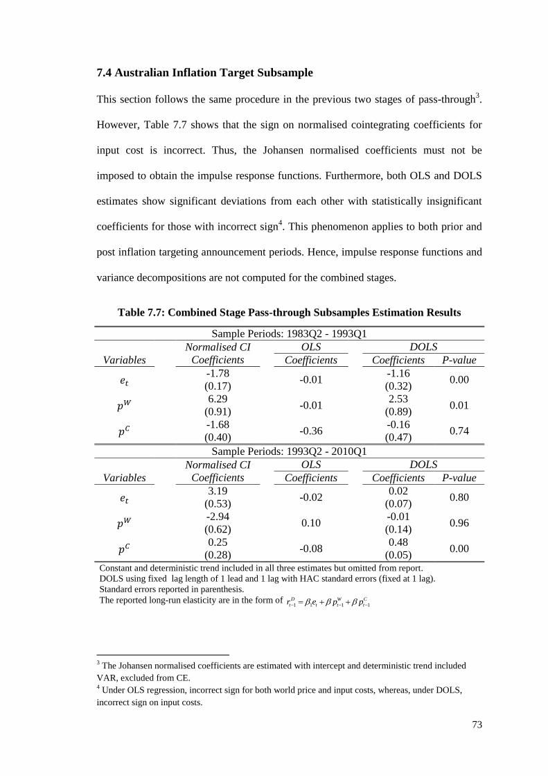
73

7.4 Australian Inflation Target Subsample

This section follows the same procedure in the previous two stages of pass-through3.

However, Table 7.7 shows that the sign on normalised cointegrating coefficients for

input cost is incorrect. Thus, the Johansen normalised coefficients must not be

imposed to obtain the impulse response functions. Furthermore, both OLS and DOLS

estimates show significant deviations from each other with statistically insignificant

coefficients for those with incorrect sign4. This phenomenon applies to both prior and

post inflation targeting announcement periods. Hence, impulse response functions and

variance decompositions are not computed for the combined stages.

Table 7.7: Combined Stage Pass-through Subsamples Estimation Results

Sample Periods: 1983Q2 - 1993Q1

Normalised CI

Coefficients

OLS DOLS

Variables Coefficients Coefficients P-value

-1.78

(0.17)

-0.01

-1.16

(0.32) 0.00

6.29

(0.91)

-0.01

2.53

(0.89) 0.01

-1.68

(0.40)

-0.36

-0.16

(0.47) 0.74

Sample Periods: 1993Q2 - 2010Q1

Normalised CI

Coefficients

OLS DOLS

Variables Coefficients Coefficients P-value

3.19

(0.53)

-0.02

0.02

(0.07) 0.80

-2.94

(0.62)

0.10

-0.01

(0.14) 0.96

0.25

(0.28)

-0.08

0.48

(0.05) 0.00


DOLS using fixed lag length of 1 lead and 1 lag with HAC standard errors (fixed at 1 lag).


The reported long-run elasticity are in the form of 1 1 1 1

D W C

t t t tr e p p

3 The Johansen normalised coefficients are estimated with intercept and deterministic trend included

VAR, excluded from CE. 4 Under OLS regression, incorrect sign for both world price and input costs, whereas, under DOLS,

incorrect sign on input costs.

74

7.6 Rolling Window for Coefficients Stability

A rolling window is also performed on combined stage pass-through with a window of

20 implemented on both Johansen and DOLS methodology. Figure 7.2 shows the

coefficient on exchange rate, world price, and input costs demonstrate more

fluctuation compared to the previous two stage of pass-through. Moreover, all three

plots show a clear structural change in the beginning of 1996, which could be caused

by the delayed effect of inflation targeting implemented by the RBA in the mid 1993.

Figure 7.2: Combined Stage Pass-through Rolling Window on DOLS Coefficients

-5

-4

-3

-2

-1

0

1

88 90 92 94 96 98 00 02 04 06 08

TWI TWI LB TWI UB

-10

-5

0

5

10

15

20

25

88 90 92 94 96 98 00 02 04 06 08

PW PW LB PW UB

-12

-8

-4

0

4

8

88 90 92 94 96 98 00 02 04 06 08

PC PC LB PC UB

75

8. Conclusion and Limitations

8.1 Conclusion

The first and second stage results show three main findings. Firstly, from the first

stage pass-through results, the speed of penetration of exchange rate shock to import

price is rapid and large in magnitude. Additionally, the long-run elasticity was

estimated to be close to unity.

The first stage results establish rapid exchange rate pass-through to the import price

over-the-docks. However, the second stage results shows limited pass-through of the

import price to the domestic retail price. Thus, another important finding is the role

played by the mark-up on cost. The subsample robustness check confirms the

increasing absorptive capacity mark-up of exchange rate fluctuations triggered by

inflation targeting. Lastly, the persistency of input costs is found to have risen, while

the retail price has fallen. A possible cause of the result may arise from the loss in

pricing power of the retailers.

The result from second stage has important policy implications for the central bank. In

addition to the knowledge of the extent and speed of pass-through, a better

understanding of the sources that caused the decline in exchange rate pass-through

would allow the central bank to improve inflation forecast, thereby, effectively achieve

the primary goal of output and price stability in the domestic economy.

Despite the empirical evidence found towards the direct impact of the exchange rate

on the domestic retail price, robustness checks are not performed, thus, conclusions on

whether inflation targeting causes any changes in the direct exchange rate pass-

through cannot be made.

76

8.2 Limitations and Future Research

Despite the results shown in the previous chapters on first and second stage, there are

several limitations to this study. One of the shortcomings involves the identification

scheme undertaken in this thesis. The method of identification relies on the presence

of only one cointegration relationship in the data, although, this may change if

different lags of VEC model were used. Hence, the number of cointegration

relationships may not be robust to change in the lags.

More importantly, the Johansen cointegration test is commonly applied in the

literature to test the presence of cointegration and determine the number of

cointegrating relationships. However, it does not inform us which variables appear to

be cointegrated. Thus, a VECM with incorrectly imposed cointegrating vector would

suffer inconsistent estimates. The approach implemented in this thesis involves, firstly,

the estimation of the equivalent reduced-form VEC model, then, the cointegrating

variable is determined through the significance of the adjustment coefficient on the

cointegrating vector. However, there appears some evidence of two cointegrating

variables. In the case of two or more cointegrating relationships, future research may

consider to adopt King et al. (1991) approach to identify only certain shocks of interest

amongst two cointegrating relationships.

Additionally, the method of imposing structural cointegration restrictions with

Choleski ordering provides a simple method of recovering structural shocks. However,

some of the imposed zero contemporaneous restrictions may be debateable in practice.

Hence, alternative identification strategy may adopt a recursive long-run identification

described in Fisher and Huh (2012) to recover sensible structural permanent shocks of

interest from reduced-form models.

77

Another issue relates to the symmetric effect of the impulse response functions

generated for exchange rate shocks. The effect of appreciation and depreciation of the

exchange rate may have different effects on the pass-through to retail price. Despite

this, the literature on nonlinear or asymmetric effects for Australia is limited and

asymmetric response of the exchange rate to the response at a retail price level is even

rarer. Dwyer and Lam (1994) attempted to split the sample of the exchange rate data in

to periods of appreciations and depreciation. However, the precision of the results are

questionable due to shortened data sample.

Another recent study conducted by Nogueira and León-Ledesma (2008), on a group of

industrialised economies, used smooth transition model to account for nonlinearity in

exchange rate pass-through to inflation. Similarly, Nogueira et al. (2010) utilised a

time-varying state-space model to account for time-varying coefficients and test the

causal relationship of whether low inflation environment imply the decline in the

exchange rate pass-through. Thus, one possible extension would be to adopt a state-

space model similar to Nogueira et al. (2010) in an Australian context. However, this

abandons the current structural framework. Instead, Markov-switching models are

popular amongst the literature to account for asymmetry in volatilities, thus, can be

used to combine with a VAR framework in an Australian context.

Another possible extension stems from the mark-up portrayed in the second stage.

Hooper and Mann (1989) first extended the typical mark-up model to incorporate

domestic and foreign competitive pressure that varies according to mark-up, which

Menon (1992), Menon (1993), and Swift (1998) later incorporated into their analytical

framework. Additionally, Dwyer and Lam (1994) predicted the mark-up, a priori, that

related to output gap. However, in this thesis, factors that controls for domestic

economic activities are not incorporated into a SVEC framework. Instead, the mark-up

78

is assumed to be the residual of input cost. Thus, future research may consider

incorporating factors that describe the behaviour of mark-up, thereby, the mark-up

would be endogenously determined.

79

Appendix 1: Data Construction

A1.1 Retail Prices of Imported Consumption Goods

The construction of retail price of import consumption goods series is based on the

Consumer Price Index (CPI) for Groups, Subgroups, and Expenditure classes as a

weighted average of 8 Australian capital cities sourced from the ABS Catalogue No.

6401.0. In conjunction with the CPI figures, the current and historical weights of

successive periods for group, sub-group, and expenditure classes of CPI are obtained

from the ABS, Catalogue No. 6431.0. All sample periods are obtained from June

quarter of 1983 to March quarter 2010.

The objective is to isolate the portion of CPI that is only attributed to imported

consumption goods as a proxy for retail price of imported consumption goods. The

first issue encountered is the decision of which groups, sub-groups or expenditure

classes are to be included or excluded from the proxy. Based on Dwyer and Lam

(1994)1, I have only included the following sub-groups and expenditure classes:

alcohol beverages, footwear, household textiles, personal care products, and motor

vehicles.

Extraction of only a subset is due to the following issues encountered. Firstly, time-

varying weights can be a source of dramatic fluctuations in the proxy. Due to

misalignment of sample periods compared to Dwyer and Lam (1994), which means

that the CPI figures would have been adjusted much more significantly predominantly

driven by technological advancement. Hence, the adjustment of weights that involves

dropping, merging, and splicing of sub-groups, expenditure classes, and even groups

1 Dwyer and Lam (1994) included the following sub-groups and expenditure classes: processed fruit and

vegetables, clothing except for dry cleaning and shoe repairs, household appliances, household textiles,

household utensils and tools, motor vehicles, tyres and tubes, alcoholic drinks, personal care products,

books , newspapers, and magazines, and recreation goods.

80

of the CPI would raise difficulty in weighting of the expenditure class across different

series defined over different time periods. More importantly, there exist numerous

missing observations for expenditure class in the CPI2. Hence, missing observations

are inevitable. This further complicates the weighting of the periods where two series

connect, due to both missing observations from re-definition of sub-groups and

expenditure classes and changes in the weighting patterns. Therefore, abnormal

fluctuations in six connecting points are observed amongst the seven series.

Historical weight patterns are typically decomposed into 7 series3. Within each series,

their subgroup and expenditure weights are multiplied against their respective

subgroup and expenditure class index over their defined periods of time. Finally,

simply aggregate across over the five mentioned subgroups and expenditure classes in

each time periods result in the proxy for retail price of consumption imported goods.

However, the removal of expenditure classes and subgroups that contain missing

values, thus, utilise only the five subgroups and expenditure classes specified causes

dramatic fluctuations. Specifically, these 'jumps' in the six connecting joints amongst

the series is eliminated using the following approach. The two points surrounding the

abnormal point is identified, averaged, and substituted for the abnormal point. The

method is repeated for all six abnormal points. The smoothed level of retail price of

imported consumption goods is obtained by rolling back from the last series

containing the June, September, and December quarters of 2011.

2 The 16th categorical index is used for all historical data.

3 According to ABS explanatory notes; 10th series corresponds to periods between 1982:03 to 1986:09,

11th series corresponds to periods between 1986:12 to 1992:03, 12th series corresponds to periods

between 1992:06 to 1998:03, 13th series corresponds to periods between 1998:06 to 2000:03, 14th

series corresponds to periods between 2000:06 to 2005:03, 15th series corresponds to periods between

2005:06 to 2011:03, and 16th series corresponds to periods between 2011:06 to 2011:12.

81

A1.2 Prices of Consumption Imports Over-the-docks

A proxy for this measure involves both import price index and weights that extract

only the imported consumption portion. Import price index is sourced from the ABS

Catalogue No. 6457.0 Australia International Trade Price Index, while the weights are

constructed from the ABS Catalogue No. 5439.0 Australia International Merchandise

Imports. Both catalogues utilise the Standard International Trade Classification (digit 1

and 2) which ensure the match across two series.

Similar to the retail price series, exclusion of items is based on Dwyer and Lam (1994)

in SITC digit 14. A simple proportional set of weights can be obtained by dividing

each category by its total and averaged over across time. The relative weights of the

remaining are remained without any further rescaling.

These weights can be used to scale SITC digit 1 index numbers for import price index.

Simply obtain the all group import price index and deduct the aggregated weighted

SITC digit 1 categories that are thought to be non-consumption goods. The remaining

portion is used as a proxy for the import price index of consumption goods.

A1.3 World Export Price for Consumption Goods

A comprehensive measure of Australia's 21 major trading partners is used to account

for world export price of consumption goods5. Each country's export price index can

be sourced from either the World Bank or the Organisation for Economic Co-

operation and Development iLibrary. The weights applied are calculated based on

4 Items that are excluded include crude materials, inedible, except fuel; mineral fuels, lubricants and

related materials; chemicals and related products; and machinery and transport equipment. 5 Countries included are: Canada, China, European Union, Hong Kong, India, Indonesia, Japan,

Malaysia, New Taiwan, New Zealand, Papua New Guinea, Singapore, South Africa, South Korea,

Sweden, Switzerland, Thailand, United Arab Emirates, United Kingdom, United States, and Vietnam.

82

averaged weights of Trade Weighted Index (TWI) sourced from the RBA Statistical

Release.

The approach used in this thesis in the construction of the weights is different to that

of the RBA research paper by Dwyer and Lam, 1994. They substituted the four-digit

Australian Standard Industrial Classification (ASIC) data for value of imports

classified by commodity and countries as the data were not available. Instead of using

the ASIC data, to be consistent with the effective exchange rate weights, the same

weights for TWI are substituted. Specifically, the longest duration of weights for TWI

for each year from 1997 to 2011 is extracted and averaged across time for each

country.

Table A1.1: Australia's Major Trading Partner TWI Weights

Country Averaged TWI

Canada 0.014

China 0.118

European Union 0.121

Hong Kong 0.020

India 0.025

Indonesia 0.029

Japan 0.167

Malaysia 0.030

New Taiwan 0.036

New Zealand 0.053

Papua New Guinea 0.012

Singapore 0.043

South Africa 0.009

South Korea 0.062

Sweden 0.009

Switzerland 0.008

Thailand 0.029

United Arab Emirates 0.011

United Kingdom 0.049

United States 0.133

Vietnam 0.014

83

One problem may arise in such computation would be mismatch in country's TWI due

to a change in trading pattern with Australia's trading partner. One clear example

would be the formulation of European Union where some countries that were initially

excluded as Australia's trading partner are now included as part of European Union.

This complication can be mitigated by excluding those periods from the average of the

country, namely; European union, United Arab Emirates, and Vietnam. Consequently,

minimal effect on final TWI is achieved. Table A1.1 highlights the averaged TWI

figures where the included countries comprised of 99.3% of total TWI in the world.

There are several challenges in the extraction of consumer export prices for each

above mentioned countries. Due to a large amount of countries and time constraints, it

is infeasible to extract total export price for each country in spite of missing data.

Hence, export price indexes are obtained for all countries in computation of world

export price.

The export price index for Asian Pacific countries are constructed by dividing export

value index with its corresponding export volume index. An issue arise due to the time

series obtained for all countries are in yearly frequency. To convert data series into

quarterly frequency, geometric linear interpolation is used to apply across two

consecutive years as the following:

4

1

i

yt

Qt yt

yt

EPIEPI EPI

EPI

(A1.1)

for . QtEPI denotes the export price index for the quarter t ,

ytEPI denotes

the export price index for the current year and 1ytEPI denotes export price index for

84

the next year. In addition, the indexation for the base period was chosen to be the year

2000, thus, all countries are adjusted in accordance to the base period6.

A further issue relates to the missing observations for both export price index and

export volume index from the World Bank for developed economies. For Japan,

export price index obtained from OECD iLibrary includes period up to and including

first quarter of 2006. The remaining data is sourced from Bank of Japan and the base

year was set to 2000. With United Kingdom, New Zealand, and Canada, export unit

value index is substituted for export price index sourced from OECD iLibrary, while,

export price index is sourced for Sweden and the United States. With Switzerland,

export unit value index is also sourced, however, the period of missing observations

between Q4 1987 to Q4 1988 is treated by application of geometric linear interpolation

between the adjacent Q3 1987 and Q1 1989.

Finally, all countries that are currently part of the European Union are included with

either the unit value index or export price index7. The resulting figures are averaged

for all time periods specified. However, missing observations are present in most of

the countries during the earlier periods. A similar approach to the treatment of TWI is

implemented where countries with periods of missing observations are excluded from

the average. Furthermore, indexation of base period is fixed at year 2000 for all

countries in the European Union.

The world price can be calculated as follows:

6 The construction of export price index and linear interpolation is applied to China, Singapore, India,

Thailand, Malaysia, Indonesia, Hong Kong, Papua New Guinea, South Korea, Vietnam, New Taiwan,

United Arab Emirates, and South Africa. 7 Countries with reported unit value index were Austria, Belgium, Denmark, Spain, Finland, France,

Hungary, Ireland, Italy, Luxembourg, and Netherlands. Countries with reported export price index are

Germany, Czech Republic, Poland, Portugal, Greece, Estonia, Bulgaria, Cyprus, Latvia, Lithuania,

Malta, Romania, and Slovenia.

85

( )i

t i t

i

W w p (A1.2)

where iw denotes the average TWI weights from the th country, i

tP denotes the export

price index of consumption goods in the th country. The proxy for world export price

of consumption aggregates the weighted export price for each country mentioned.

A1.4 Nominal Effective Exchange Rate

The nominal effective exchange rate consists of average value for Australia's currency

movement with that of its 21 major trading partners sourced from monthly nominal

TWI in the RBA Statistic Table. These monthly series are transformed into quarterly

figures by retaining the last month for each quarter. Lastly, the indexation of base

period is fixed in the year 2000.

A1.4 Costs Borne By Importers and Retailers

The major input costs faced by importers and retailers were categorised into five major

sub-groups, namely: international freight cost, taxes on international trade, unit labour

costs, domestic transport cost, and other expenses. This is the same categories defined

by Dwyer and Lam (1994) and it is noted that these costs do not exhaustively contain

all costs. Cost such as utility charges account for a small proportion with less

fluctuations.

1) International freight cost

International freight is sourced from the ABS Catalogue No. 5302.0 Australia Balance

of Payment and International Investment Position. The required sample of Q2 1983 to

Q1 2010 is sourced from the past and current releases of freight on imports under

transportation. The last quarter value for each balance of payment in the current

account with seasonal adjusted figures ($million) are extracted.

86

To achieve consistency for all costs, the price of international freight are re-based to

year 2000 (=100). However, due to the quarterly data, the year 2000 values are

averaged and indexed according to this figure.

2) Taxes on international trade cost

Tax on international trade was sourced from the ABS Catalogue No. 5206 Australian

National Accounts: National Income, Expenditure and Product. The seasonally

adjusted tax on international trade in millions ($) is sourced and re-based to year 2000

(=100), similar to international freight costs. Following Dwyer and Lam (1994), tax on

international trade was used to calculate average tariff rate, which is to be included in

to import price index for second stage pass-through. Average tariff is calculated as

value of custom duties in proportion to import values.

3) Unit labour cost

Unit labour cost is sourced from the ABS Catalogue No. 5206 Australian National

Accounts: National Income, Expenditure and Product. Seasonally adjusted, non-farm,

nominal unit labour index is extracted for the specified sample period. This was re-

based to 2000 (=100).

4) Domestic freight

A measure of domestic freight cost involves the index of prices paid by farmers to

transport from the farm to either the docks or stores. This is sourced from the

Australian Bureau of Agricultural and Resource Economics' (ABARE) current and

past publications of Australian Agricultural Commodity Statistics. Specifically, under

the indexes of prices paid by farmers in farmers input, the previous year's figure of

freight outward in marketing is extracted from each current year's publication.

87

The latest figure for each publication, similar to that of international freight cost, is

extracted to overcome the problem of variant figures. To transform the yearly figures,

geometric linear interpolation is applied to obtain the required interpolated quarterly

frequency. Furthermore, the index is re-based from year 1997 to 2000 (=100).

5) Other expenses

Other expenses are pooled together from different retail business operations and

industrial performance surveys sourced from the ABS Catalogue No. 8140.0.

Specifically, the averaged expense for retail trade industry is extracted. Variant

averaged expense cost is treated similarly to that of domestic freight and international

freight. Likewise to the other costs, the obtained figure is re-based to year 2000 (=100).

Estimates of cost share that are used to weight the cost index are sourced from the

reported cost shares by Dwyer and Lam (1994). They constructed the figure from

various publications including the Manufacturing Census, Retail and Business

Operations and Industry Performance. Weighted cost index is simply an aggregate of

cost index as a proportion of its cost weights.

Table A1.2: Cost Index Weights

Major Costs Weight for Cost Index

International Freight 0.17

Unit Labour Cost 0.62

Domestics Freight 0.13

Other Expenses 0.08

Total 1.00

88

Appendix 2: Reduced-form Level VAR Lag Selection

The selection of suitable number of lags to include in the reduced-form VAR level

model is based on lags that are sufficient in removal of serial correlation in the residual

of the model. Maximum lags to include in VAR estimation are capped to six for all

stages because of limited data sample, higher lag levels reduce the degrees of freedom

and for parsimonious reasons.

The selection of VAR lags are achieved in two steps:

1. Use various selection criteria as a guide to determine the maximum lags to be

included.

2. Compare the competing VAR models selected from previous selection criteria

and choose the most parsimonious model that removes serial correlation

amongst the residuals.

The results from Table A2.1 shows a series of lag length selection criterions for first,

second, and combined stage pass-through. Table A2.2 shows the LM test of residual

serial correlation for two competing VAR models in each stage.

For the first stage, two selection criterions select a VAR(2) model while the rest

selects lag length above VAR(6). However, VAR(2) and VAR(3) is compared for

parsimonious reason. From Table A2.2, VAR(3) seems to be the best model which

shows serially uncorrelated residuals by the LM statistics at 5% level, except for the

second lag.

Both second and combined stage lag length selection criterions choose either VAR(2)

or VAR(3), thus, the serial correlation of the two competing models provide the

deciding factor of optimal model. Table A2.2 shows VAR(3) model are the optimal

89

model for both second and combined stage pass-through with serially uncorrelated

residuals shown for all lags up to the sixth lag. Hence, VAR(3) model is chosen to be

the optimal model for all three stages of pass-through.

Table A2.1: Level VAR Lag Length Selection Criterions

First stage pass-through

Lag LogL LR FPE AIC SC HQ

0 306.54 - 3.60e-07 -6.32 -6.24 -6.29

1 632.13 624.05 4.92e-10 -12.92 -12.60 -12.79

2 658.89 49.61 3.40e-10 -13.29 -12.73* -13.06*

3 671.19 22.05 3.18e-10 -13.36 -12.56 -13.03

4 677.27 10.51 3.39e-10 -13.30 -12.26 -12.88

5 681.91 7.73 3.73e-10 -13.21 -11.92 -12.69

6 685.27 5.38 4.22e-10 -13.09 -11.57 -12.47

Second stage pass-through


0 250.23 - 1.57e-06 -4.85 -4.77 -4.82

1 797.84 1052.27 4.08e-11 -15.41 -15.10* -15.28

2 817.28 36.20 3.33e-11 -15.61 -15.07 -15.39*

3 830.44 23.74* 3.07e-11* -15.69* -14.92 -15.38

4 833.73 5.75 3.44e-11 -15.58 -14.58 -15.18

5 839.30 9.40 3.69e-11 -15.52 -14.28 -15.02

6 842.35 4.96 4.17e-11 -15.40 -13.93 -14.81

Combined stage pass-through


0 433.47 - 2.59e-09 -8.42 -8.32 -8.38

1 1128.99 1322.85 4.23e-15 -21.74 -21.23* -21.54

2 1160.38 57.25 3.13e-15 -22.05 -21.12 -21.67*

3 1176.69 28.46* 3.13e-15* -22.05* -20.71 -21.51

4 1188.22 19.22 3.44e-15 -21.97 -20.22 -21.26

5 1195.10 10.91 4.16e-15 -21.79 -19.62 -20.91

6 1206.29 16.91 4.65e-15 -21.69 -19.12 -20.65

90

Table A2.2: Level VAR Residual Serial Correlation LM Test

First stage pass-through

Lags LM stat P-Value

VAR(2) 1 17.22 0.05

2 30.55 0.00

3 4.55 0.87

4 5.24 0.81

5 5.15 0.82

6 11.67 0.23

VAR(3) 1 12.53 0.19

2 20.05 0.02

3 9.54 0.39

4 15.52 0.08

5 6.50 0.69

6 9.29 0.41

Second-stage pass-through


VAR(2) 1 25.71 0.00

2 18.81 0.03

3 8.57 0.48

4 7.95 0.54

5 10.65 0.30

6 6.08 0.73

VAR(3) 1 6.60 0.68

2 8.83 0.45

3 6.91 0.65

4 9.06 0.43

5 6.18 0.72

6 5.94 0.75

Combined stage pass-through


VAR(2) 1 31.77 0.01

2 37.18 0.00

3 15.56 0.48

4 16.60 0.41

5 15.42 0.49

6 18.52 0.29

VAR(3) 1 21.48 0.16

2 15.78 0.47

3 16.46 0.42

4 10.87 0.82

5 14.69 0.55

6 19.19 0.26

91

Appendix 3: Further Test for Cointegration

Additional to the Engle-Granger and Johansen Cointegration methodology, another

possible test for cointegration involves testing the significance of the error correction

term in a Error Correction Model (ECM). This was adopted by Dwyer et al. (1993)

and derived from Kremers et al. (1992), where the authors argue that such test have

more power than the residual based test implied by Engle-Granger. However, the

drawback of such test involves, a priori, of the cointegrating variable.

The ECM for first, second, and combined stage pass-through are computed using

maximum lag of 4 where insignificant lags are removed from the model1. Table A3.1

shows the estimated adjustment coefficients for each of the pass-through stages. The

results show statistically significant coefficient at 5% level for the first and second

stage, however, this is not the case for the combined stage pass-through.

Table A3.1: Significance of Error Correction Term Test

First stage ECM

Variable Coefficient T stats P-value

1

D

tp

-0.14

(0.04) -3.47 0.00

Second stage ECM

Variable

Coefficient T stats P-value

1

D

tr

-0.02

(0.01) -2.37 0.02

Combined stage ECM

Variable

Coefficient T stats P-value

-0.01

(0.01) -1.35 0.18

1 For second stage, contemporaneous import price and input cost are included even though, the

coefficients are statistically insignificant. For combined stage, both contemporaneous world price and

input cost are included, although, their respective coefficients are estimated to be statistically

insignificant.

1

D

tr

92

Appendix 4: Approximate 2 Standard Error Bands Based on Levels

VAR

93


Full Sample


1983Q2-1993Q1

-.06

-.04

-.02

.00

.02

.04

.06

2 4 6 8 10 12 14 16 18 20 22 24

Response of PW to PW

-.06

-.04

-.02

.00

.02

.04

.06

2 4 6 8 10 12 14 16 18 20 22 24

Response of PW to TWI

-.06

-.04

-.02

.00

.02

.04

.06

2 4 6 8 10 12 14 16 18 20 22 24

Response of PW to PD

-.06

-.04

-.02

.00

.02

.04

.06

2 4 6 8 10 12 14 16 18 20 22 24

Response of TWI to PW

-.06

-.04

-.02

.00

.02

.04

.06

2 4 6 8 10 12 14 16 18 20 22 24

Response of TWI to TWI

-.06

-.04

-.02

.00

.02

.04

.06

2 4 6 8 10 12 14 16 18 20 22 24

Response of TWI to PD

-.06

-.04

-.02

.00

.02

.04

.06

2 4 6 8 10 12 14 16 18 20 22 24

Response of PD to PW

-.06

-.04

-.02

.00

.02

.04

.06

2 4 6 8 10 12 14 16 18 20 22 24

Response of PD to TWI

-.06

-.04

-.02

.00

.02

.04

.06

2 4 6 8 10 12 14 16 18 20 22 24

Response of PD to PD

-.10

-.05

.00

.05

.10

2 4 6 8 10 12 14 16 18 20 22 24


-.10

-.05

.00

.05

.10

2 4 6 8 10 12 14 16 18 20 22 24


-.10

-.05

.00

.05

.10

2 4 6 8 10 12 14 16 18 20 22 24


-.10

-.05

.00

.05

.10

2 4 6 8 10 12 14 16 18 20 22 24


-.10

-.05

.00

.05

.10

2 4 6 8 10 12 14 16 18 20 22 24


-.10

-.05

.00

.05

.10

2 4 6 8 10 12 14 16 18 20 22 24


-.10

-.05

.00

.05

.10

2 4 6 8 10 12 14 16 18 20 22 24


-.10

-.05

.00

.05

.10

2 4 6 8 10 12 14 16 18 20 22 24


-.10

-.05

.00

.05

.10

2 4 6 8 10 12 14 16 18 20 22 24


94


1993Q2-2010Q1

Figure A4.4: Second Stage Pass-through Impulse Response Functions From

VAR(3): Full Sample

-.10

-.05

.00

.05

.10

2 4 6 8 10 12 14 16 18 20 22 24


-.10

-.05

.00

.05

.10

2 4 6 8 10 12 14 16 18 20 22 24


-.10

-.05

.00

.05

.10

2 4 6 8 10 12 14 16 18 20 22 24


-.10

-.05

.00

.05

.10

2 4 6 8 10 12 14 16 18 20 22 24


-.10

-.05

.00

.05

.10

2 4 6 8 10 12 14 16 18 20 22 24


-.10

-.05

.00

.05

.10

2 4 6 8 10 12 14 16 18 20 22 24


-.10

-.05

.00

.05

.10

2 4 6 8 10 12 14 16 18 20 22 24


-.10

-.05

.00

.05

.10

2 4 6 8 10 12 14 16 18 20 22 24


-.10

-.05

.00

.05

.10

2 4 6 8 10 12 14 16 18 20 22 24


-.08

-.04

.00

.04

.08

5 10 15 20 25 30 35 40 45 50

Response of PT to PT

-.08

-.04

.00

.04

.08

5 10 15 20 25 30 35 40 45 50

Response of PT to RPI

-.08

-.04

.00

.04

.08

5 10 15 20 25 30 35 40 45 50

Response of PT to PC

-.08

-.04

.00

.04

.08

5 10 15 20 25 30 35 40 45 50

Response of RPI to PT

-.08

-.04

.00

.04

.08

5 10 15 20 25 30 35 40 45 50

Response of RPI to RPI

-.08

-.04

.00

.04

.08

5 10 15 20 25 30 35 40 45 50

Response of RPI to PC

-.08

-.04

.00

.04

.08

5 10 15 20 25 30 35 40 45 50

Response of PC to PT

-.08

-.04

.00

.04

.08

5 10 15 20 25 30 35 40 45 50

Response of PC to RPI

-.08

-.04

.00

.04

.08

5 10 15 20 25 30 35 40 45 50

Response of PC to PC

95


VAR(3) With Ordering Implied by DOLS Estimates: 1983Q2-1993Q1


VAR(3) With Ordering Implied By Johansen Normalised Coefficients: 1983Q2-

1993Q1

-.08

-.04

.00

.04

.08

1 2 3 4 5 6 7 8 9 10


-.08

-.04

.00

.04

.08

1 2 3 4 5 6 7 8 9 10


-.08

-.04

.00

.04

.08

1 2 3 4 5 6 7 8 9 10


-.08

-.04

.00

.04

.08

1 2 3 4 5 6 7 8 9 10


-.08

-.04

.00

.04

.08

1 2 3 4 5 6 7 8 9 10


-.08

-.04

.00

.04

.08

1 2 3 4 5 6 7 8 9 10


-.08

-.04

.00

.04

.08

1 2 3 4 5 6 7 8 9 10


-.08

-.04

.00

.04

.08

1 2 3 4 5 6 7 8 9 10


-.08

-.04

.00

.04

.08

1 2 3 4 5 6 7 8 9 10


-.04

-.02

.00

.02

.04

.06

.08

1 2 3 4 5 6 7 8 9 10


-.04

-.02

.00

.02

.04

.06

.08

1 2 3 4 5 6 7 8 9 10


-.04

-.02

.00

.02

.04

.06

.08

1 2 3 4 5 6 7 8 9 10


-.04

-.02

.00

.02

.04

.06

.08

1 2 3 4 5 6 7 8 9 10


-.04

-.02

.00

.02

.04

.06

.08

1 2 3 4 5 6 7 8 9 10


-.04

-.02

.00

.02

.04

.06

.08

1 2 3 4 5 6 7 8 9 10


-.04

-.02

.00

.02

.04

.06

.08

1 2 3 4 5 6 7 8 9 10


-.04

-.02

.00

.02

.04

.06

.08

1 2 3 4 5 6 7 8 9 10


-.04

-.02

.00

.02

.04

.06

.08

1 2 3 4 5 6 7 8 9 10


96


VAR(3) With Ordering Implied By Johansen Normalised Coefficients: 1993Q2-

2010Q1

-.08

-.04

.00

.04

.08

.12

2 4 6 8 10 12 14 16 18 20 22 24


-.08

-.04

.00

.04

.08

.12

2 4 6 8 10 12 14 16 18 20 22 24


-.08

-.04

.00

.04

.08

.12

2 4 6 8 10 12 14 16 18 20 22 24


-.08

-.04

.00

.04

.08

.12

2 4 6 8 10 12 14 16 18 20 22 24


-.08

-.04

.00

.04

.08

.12

2 4 6 8 10 12 14 16 18 20 22 24


-.08

-.04

.00

.04

.08

.12

2 4 6 8 10 12 14 16 18 20 22 24


-.08

-.04

.00

.04

.08

.12

2 4 6 8 10 12 14 16 18 20 22 24


-.08

-.04

.00

.04

.08

.12

2 4 6 8 10 12 14 16 18 20 22 24


-.08

-.04

.00

.04

.08

.12

2 4 6 8 10 12 14 16 18 20 22 24


97

Figure A4.8: Combined Stage Pass-through Impulse Response Functions From VAR(3) With Ordering Implied By Johansen

Normalised Coefficients: Full Sample

-.08

-.04

.00

.04

.08

2 4 6 8 10 12 14 16 18 20 22 24


-.08

-.04

.00

.04

.08

2 4 6 8 10 12 14 16 18 20 22 24


-.08

-.04

.00

.04

.08

2 4 6 8 10 12 14 16 18 20 22 24

Response of PW to PC

-.08

-.04

.00

.04

.08

2 4 6 8 10 12 14 16 18 20 22 24

Response of PW to RPI

-.08

-.04

.00

.04

.08

2 4 6 8 10 12 14 16 18 20 22 24


-.08

-.04

.00

.04

.08

2 4 6 8 10 12 14 16 18 20 22 24


-.08

-.04

.00

.04

.08

2 4 6 8 10 12 14 16 18 20 22 24

Response of TWI to PC

-.08

-.04

.00

.04

.08

2 4 6 8 10 12 14 16 18 20 22 24

Response of TWI to RPI

-.08

-.04

.00

.04

.08

2 4 6 8 10 12 14 16 18 20 22 24

Response of PC to PW

-.08

-.04

.00

.04

.08

2 4 6 8 10 12 14 16 18 20 22 24

Response of PC to TWI

-.08

-.04

.00

.04

.08

2 4 6 8 10 12 14 16 18 20 22 24


-.08

-.04

.00

.04

.08

2 4 6 8 10 12 14 16 18 20 22 24


-.08

-.04

.00

.04

.08

2 4 6 8 10 12 14 16 18 20 22 24

Response of RPI to PW

-.08

-.04

.00

.04

.08

2 4 6 8 10 12 14 16 18 20 22 24

Response of RPI to TWI

-.08

-.04

.00

.04

.08

2 4 6 8 10 12 14 16 18 20 22 24


-.08

-.04

.00

.04

.08

2 4 6 8 10 12 14 16 18 20 22 24


98

Appendix 5: Data Properties and Model Estimation for Subsamples

This appendix shows the results from subsample estimation for the second stage pass-

through. Table A5.1-A5.3 shows the first stage model estimation from VECM (2) and

regression coefficients implied by Johansen, OLS, and DOLS. Table A5.4-A5.8 shows

the second stage model estimation with regression estimates implied from Johansen,

OLS, and DOLS.

From the first stage pass-through, long-run coefficients for the first subsample

presented in Table A5.1 show correct signs for all three methodologies. However, the

magnitude on Johansen normalised coefficients are slightly higher than complete pass-

through. Thus, the DOLS estimates are replaced instead to generate impulse response

functions. Furthermore, the long-run coefficients for the post inflation targeting

announcement subsample show consistently incorrect sign on Johansen, OLS, and

DOLS coefficients. Hence, DOLS estimates from the subsample 1983Q2- 1993Q1

were substituted instead.

For the second stage pass-through, Table A5.4 shows the long-run coefficients for

prior inflation targeting subsample. All coefficients reported from the three

methodologies have correct signs. Thus, Johansen normalised coefficients are used to

generate impulse response function, while DOLS estimates were used as a robustness

check. The corresponding model estimation for adjustment coefficients are reported in

Table A5.5 and A5.6. For the post inflation targeting subsample, Johansen normalised

coefficient on the after-tax import price are incorrect, thus, DOLS estimates are

substituted instead.

99

Table A5.1: First Stage Pass-through Estimation Results: 1983Q2-1993Q1

Variables

Normalised CI

Coefficients

OLS DOLS



te -1.52

(0.12)

-1.15

(0.04) 0.00

-0.87

(0.05) 0.00

W

tp 1.27

(0.31)

0.91

(0.11) 0.00

1.24

(0.08) 0.00


DOLS using AIC (Max lag length 5) lag and lead both equal to five with HAC standard errors (fixed

4 lags).



D W

t t tp e p

Table A5.2: First Stage Pass-through Adjustment Coefficients on Error

Correction of VECM(2) Implied By DOLS Estimates: 1983Q2 - 1993Q1

Dependent

Variable

Independent


D

tp 1tec -0.15

(0.04) -3.89**

te 0.17

(0.10) 1.70

W

tp -0.001

(0.02) -0.08



Error correction term is defined as 1 1 1 10.87 1.24 2.31D W

t t t tec p e p using DOLS estimated coefficients

from Table A5.1.

Table A5.3: First Stage Pass-through Estimation Results: 1993Q2 - 2010Q1

Variables

Normalised CI

Coefficients

OLS DOLS



te -0.47

(0.20)

-0.41

(0.14) 0.00

-0.34

(0.18) 0.07

W

tp -0.13

(0.25)

-0.53

(0.40) 0.19

-0.61

(0.22) 0.01


DOLS using AIC (Max lag length 5) lag and lead both equal to five with HAC standard errors (fixed

4 lags).



D W

t t tp e p

1tec

1tec

100

Table A5.4: Second Stage Pass-through Estimation Results: 1983Q2 - 1993Q1

Variables

Normalised CI

Coefficients

OLS DOLS



T

tp 0.78

(0.07)

0.70

(0.06) 0.00

0.61

(0.04) 0.00

C

tp 0.15

(0.15)

0.71

(0.07) 0.00

0.69

(0.03) 0.00



1 lag).



D T C

t t tr p p

Table A5.5: Second Stage Pass-through Adjustment Coefficients on Error


Dependent

Variable

Independent


D

tr 1tec -0.03

(0.03) -0.95

T

tp -0.23

(0.23) -1.01

C

tp 0.35

(0.17) 2.11*





coefficients from Table A5.4.


Correction of VECM(2) Implied By Johansen Normalised Coefficients: 1983Q2 -

1993Q1

Dependent

Variable

Independent


D

tr 1tec -0.08

(0.02) -3.71**

T

tp -0.13

(0.19) -0.68

C

tp 0.18

(0.14) 1.32






1tec

1tec

1tec

1tec

101

Table A5.7: Second Stage Pass-through Estimation Results: 1993Q2 - 2010Q1

Variables

Normalised CI

Coefficients

OLS DOLS



T

tp -0.13

(0.09)

0.01

(0.03) 0.82

0.02

(0.07) 0.76

C

tp 0.43

(0.07)

0.48

(0.05) 0.00

0.49

(0.06) 0.00


DOLS using AIC (Max lag length 5) lag =5 and lead =1 with HAC standard errors (fixed 1 lag).



D T C

t t tr p p



Dependent

Variable

Independent


D

tr 1tec -0.08

(0.02) -3.69**

T

tp 0.01

(0.26) 0.02

C

tp -0.05

(0.09) -0.52






1tec

1tec

102

Appendix 6: Impulse Response Functions for Further Robustness

Tests

As an additional robustness check, deterministic trend is included into either the

Johansen normalised coefficients or DOLS estimates to generate the impulse response

functions for the main results presented for both the first and second stage pass-

through. Figure 6.1 presents the impulse response functions for the first stage pass-

through with estimates from the Johansen normalised coefficients. Figure 6.2 presents

the impulse response functions generated from DOLS estimates for the second stage

pass-through. Both sets of impulse response functions show consistent results to their

respective main results. Lastly, Figure 6.3 shows the second stage impulse response

functions implied by Johansen normalised coefficients.

Figure A6.1: First Stage Pass-through Impulse Response Functions on VECM(2)

Implied By Johansen Normalised Estimates: Full Sample

-.06%

-.04%

-.02%

.00%

.02%

.04%

.06%

2 4 6 8 10 12 14 16 18 20 22 24




-.06%

-.04%

-.02%

.00%

.02%

.04%

.06%

2 4 6 8 10 12 14 16 18 20 22 24




-.06%

-.04%

-.02%

.00%

.02%

.04%

.06%

2 4 6 8 10 12 14 16 18 20 22 24




103

Figure A6.2: Second Stage Pass-through Impulse Response Functions on

VECM(2) Implied By DOLS Estimates: Full Sample

Figure A6.3: Impulse Responses for One Standard Deviation Permanent and

Transitory Shocks With Johansen Normalised Coefficients: 1983Q2-1993Q1

-.04%

.00%

.04%

.08%

10 20 30 40 50 60 70 80 90 100




-.04%

.00%

.04%

.08%

10 20 30 40 50 60 70 80 90 100




-.04%

.00%

.04%

.08%

10 20 30 40 50 60 70 80 90 100




-.02%

.00%

.02%

.04%

.06%

10 20 30 40 50 60 70 80 90 100




-.02%

.00%

.02%

.04%

.06%

10 20 30 40 50 60 70 80 90 100




-.02%

.00%

.02%

.04%

.06%

10 20 30 40 50 60 70 80 90 100




104

Appendix 7: Rolling Window for Coefficient Stability

Figure A7.1: First Stage Johansen Normalised Cointegrating Coefficients

Figure A7.2: Second Stage Johansen Normalised Cointegrating Coefficients

Figure A7.3: Combined Stage Johansen Normalised Cointegrating Coefficients

-20

-10

0

10

20

30

40

88 90 92 94 96 98 00 02 04 06 08

TWI TWI LB TWI UB

-60

-50

-40

-30

-20

-10

0

10

20

30

88 90 92 94 96 98 00 02 04 06 08

WP WP LB WP UB

-100

0

100

200

300

400

500

600

88 90 92 94 96 98 00 02 04 06 08

PT PT LB PT UB

-100

0

100

200

300

400

500

88 90 92 94 96 98 00 02 04 06 08

PC PC LB PC UB

-100

0

100

200

300

400

88 90 92 94 96 98 00 02 04 06 08

TWI TWI LB TWI UB

-2,500

-2,000

-1,500

-1,000

-500

0

500

88 90 92 94 96 98 00 02 04 06 08

PW PW LB PW UB

-200

0

200

400

600

800

1,000

88 90 92 94 96 98 00 02 04 06 08

PC PC LB PC UB

105

Bibliography

Australian Bureau of Agricultural and Resource Economics, Australian Agricultural

Commodity Statistics, viewed 10 May 2012,

<http://www.daff.gov.au/abares/publications_remote_content/publication_series/austra

lian_commodity_statistics>.

Australian Bureau of Statistics, Statistics, viewed 19 March 2012,

<http://www.abs.gov.au/AUSSTATS>.

Bailliu, J, Dong, W & Murray, J 2010, "Has exchange rate pass-through really

declined? Some recent insights from the literature", Bank of Canada Review, Autumn,

pp 1-8.

Blanchard, OJ & Quah, D 1989, "The dynamic effects of aggregated supply and

aggregated demand disturbances", American Economic Review 79(4) pp 655-673.

Campa, JM & Goldberg, LS 2002, "Exchange rate pass-through into import prices: A

macro or micro phenomenon?", National Bureau of Economic Research Working

Paper Series, 8934.

Campa, JM, Goldberg, LS, González-Mínguez, JM 2005, "Exchange rate pass-through

to import price in the Euro Area", Federal Reserve Bank of New York Staff Paper, No.

219.

Campa, JM & Goldberg, LS 2006a, "Distribution margins, imported inputs, and the

sensitivity of the CPI to exchange rates", Federal Reserve Bank of New York Staff

Paper, No. 247.

Campa, JM & Goldberg, LS 2006b, "Pass-through of exchange rates to consumption

prices: What has changed and why?", in Ito, T & Rose, AT (eds), International

Financial Issues in the Pacific Rim: Global Imbalances, Financial Liberalisation, and

Exchange Rate Policy, East Asia Seminar on Economics 17. Chicago: University of

Chicago Press and NBER.

Chen, X 2010, "External shocks, monetary policy and inflation in Australia", Honours

thesis, School of Economics, University of New South Wales.

http://www.daff.gov.au/abares/publications_remote_content/publication_series/australian_commodity_statistics

http://www.daff.gov.au/abares/publications_remote_content/publication_series/australian_commodity_statistics

http://www.abs.gov.au/AUSSTATS

106

Choudhri, EU & Hakura, DS 2006, "Exchange rate pass-through to domestic prices:

Does the inflationary environment matter?", Journal of International Money and

Finance 25, pp 614-639.

Chung, E, Kohler, M & Lewis K 2011, "The exchange rate and consumer prices",

Reserve Bank of Australia Bulletin, September 2011, viewed 13 October 2012

<http://www.rba.gov.au/publications/bulletin/2011/sep/pdf/bu-0911-2.pdf>.

D'Arcy, P, Norman, D & Shan, S 2012, "Costs and margins in the retail supply chain",

Reserve Bank of Australia Bulletin, June 2012, viewed 13 October 2012

<http://www.rba.gov.au/publications/bulletin/2012/jun/pdf/bu-0612-2.pdf>.

Dwyer, J, Kent, C & Pease, A 1993, " Exchange rate pass-through: The different

responses of importers and exporters", Reserve Bank of Australia Research Discussion

Paper, No. 9304.

Dwyer, J & Lam, R 1994, "Explaining import price inflation: A recent history of

second stage pass-through", Reserve Bank of Australia Research Discussion Paper,

No. 9407.

Dwyer, J & Leong, K 2001, "Changes in the determinants of inflation in Australia",

Reserve Bank of Australia Research Discussion Paper, 2001-02.

Enders, W 2009, Applied Econometric Time Series, 3rd

edn, Wiley, United States of

America.

Faruqee, H 2004, "Exchange rate pass-through in the Euro Area: The role of

asymmetric pricing behaviour", International Monetary Fund Working Paper, No.

04/14.

Fisher LA & Huh, H 2012, "Identification methods in vector-error correction models:

Equivalence results", Journal of Economic Surveys, viewed 18 October 2012,

DOI: 10.1111/j.1467-6419.2012.00734.x.

Goldberg, PK & Knetter MM 1997, "Goods prices and exchange rates: What have we

learned?", Journal of Economic Literature, 35(3), pp 1243-1272.

http://www.rba.gov.au/publications/bulletin/2011/sep/pdf/bu-0911-2.pdf

http://www.rba.gov.au/publications/bulletin/2012/jun/pdf/bu-0612-2.pdf

107

Gonzalo, J & Ng, S 2001, "A systematic framework for analyzing the dynamic effects

of permanent and transitory shocks", Journal of Economic Dynamics and Control,

25(10), pp 1527-1546.

Hahn, E 2003, "Pass-through of external shocks to Euro Area inflation", European

Central Bank Working Paper, No. 243.

Heath, A, Roberts, I & Bulman, T 2004, "Inflation in Australia: Measurement and

modelling", in Kent, C & Guttmann, S (eds), The Future of Inflation Targeting,

Reserve Bank of Australia, pp 167-207.

Hendry, D & Krolzig, H 2001, Automatic Econometric Model Selection Using PcGets,

London: Timberlake.

Hooper, P & Mann, CL 1989, "Exchange rate pass-through in the 1980s: The case of

U.S. imports of manufactures", Brookings Papers on Economic Activity, 1, pp 297-337.

Hüfner, FP & Schröder, M 2002, "Exchange rate pass-through to consumer prices: A

European perspective", Centre for European Economic Research Discussion Paper,

No. 02-20.

Ihrig, EJ, Marazzi, M & Rothenberg AD, "Exchange rate pass-through in the G7

countries", International Finance Discussion Paper, No. 851, Federal Reserve Board

of Governors.

Ito, T, Sasaki, YN & Sato, K 2005, "Pass-through of exchange rate changes and

macroeconomic shocks to domestic inflation in East Asian countries", Research

Institute of Economy, Trade and Industry Discussion Paper Series 05-E-020.

Johansen, S 1988, "Statistical analysis of cointegration vectors", Journal of Economic

Dynamics and Control, 12(2), pp 231-254.

Junttila, J & Korhonen, M 2012, "The role of inflation regime in the exchange rate

pass-through to import prices", International Review of Economics and Finance 24, pp

88-96.

Kilian, L 2011, "Structural Vector Autoregressions", Handbook of Research Methods

and Applications on Empirical Macroeconomics, Edward Elger.

108

King, RG, Plosser, CI, Stock, JH & Watson, MW 1991, "Stochastic trends and

economic fluctuations", National Bureau of Economic Research Working Paper Series,

No. 2229.

Kremers, JM, Ericsson, NR, Dolado, JJ 1992, "The power of cointegration tests",

International Finance Discussion Papers, No. 431.

Krugman, P 1987, "Pricing to market when the exchange rate changes", in Arndt, SW

& Richardson, JD (eds), Real-financial linkages among open economies, Cambridge:

MIT Press, 1987, pp 49-70.

Lettau, M & Ludvigson, SC 2004, "Understanding trend and cycle in asset values:

Reevaluating the wealth effect on consumption", American Economic Review 94(1),

pp 276-299.

Manalo, JM 2011, "Australia's floating exchange rates: Shock absorbers or sources of

shocks?", Honours thesis, School of Economics, University of New South Wales.

Marazzi, M, Sheets, N & Vigfusson, R et al. 2005, "Exchange rate pass-through to US

import prices: Some new evidence", International Finance Discussion Paper, No. 833,

Federal Reserve Board of Governors.

McCarthy, J 2000, "Pass-through of exchange rates and import prices to domestic

inflation in some industrialised economies", Federal Reserve Bank of New York Staff

Report, 111.

Menon, J 1992, "Exchange rates and prices of Australian manufactured exports",

Weltwirtschaftliches Archiv, 128(4), pp 695-710.

Menon, J 1993, "Exchange rate pass-through: Australian imports of motor vehicles",

International Economic Journal, 7(3), pp 93-107.

Murray, J 2008, "Some puzzles related to exchange rate pass-through", mimeo, Bank

of Canada.

Nogueira Júnior, RP & León-Ledesma, MA 2008, "Exchange rate pass-through into

inflation: The role of asymmetries and nonlinearities", Studies in Economics 0801,

University of Kent.

http://link.springer.com/journal/10290

109

Nogueira Júnior, RP, León-Ledesma, MA & Reginaldo, P 2010, "Is low inflation

really causing the decline in exchange rate pass-through?", School of Economics

Discussion Papers, No. 10,02, University of Kent.

Norman, D & Richards, A 2010, "Modelling inflation in Australia", Reserve Bank of

Australia Research Discussion Paper, 2010-03.

Organisation for Economic Cooperation and Development, Monthly Statistics of

International Trade, viewed 21 April 2012,

<http://www.oecd-ilibrary.org/trade/data/monthly-statistics-of-international-

trade_msit-data-en>.

Pagan, AR & Pearson, MH 2008, "Econometric analysis of structural systems with

permanent and transitory shocks", Journal of Economic Dynamics and Control, 32(10),

pp 3376-3395.

Reserve Bank of Australia, Statistics Table, viewed 11 April 2012,

<http://www.rba.gov.au/statistics/tables/index.html>.

Sims, CA 1980, "Macroeconomics and reality", Econometrica, 48(1) pp 1-48.

Swift, R 1998, "Exchange rate pass-through: How much do exchange rate changes

affect the prices of Australian exports?", Australian Economic Papers, 37(2), pp 169-

184.

Taylor, JB 2000, "Low inflation, pass-through, and the pricing power of firms",

European Economic Review, 44(7) 1389-1408.

The World Bank, Data, viewed 21 April 2012, <http://data.worldbank.org/indicator>.

http://www.oecd-ilibrary.org/trade/data/monthly-statistics-of-international-trade_msit-data-en

http://www.oecd-ilibrary.org/trade/data/monthly-statistics-of-international-trade_msit-data-en

http://www.rba.gov.au/statistics/tables/index.html

http://data.worldbank.org/indicator

SCHOOL OF ECONOMICS - UNSW Business School · SCHOOL OF ECONOMICS HONOURS THESIS ... Jahanzeb Khan...

Documents

Transcript of SCHOOL OF ECONOMICS - UNSW Business School · SCHOOL OF ECONOMICS HONOURS THESIS ... Jahanzeb Khan...