School of Distance Education - Official website of Calicut ... STATISTICS IV Semester COMPLEMENTARY...
83
APPL COM B S UNIVE SCHOO Calicut Univer LIED STATISTI IV Semester MPLEMENTARY COURSE Sc MATHEMATICS (2011 Admission) ERSITY OF CALICU OL OF DISTANCE EDUCATION ersity P.O. Malappuram, Kerala, India 673 418 ICS UT 635
-
Upload
phungkhanh -
Category
Documents
-
view
226 -
download
2
Transcript of School of Distance Education - Official website of Calicut ... STATISTICS IV Semester COMPLEMENTARY...

APPLIED STATISTICS
IV Semester
COMPLEMENTARY COURSE
B Sc MATHEMATICS
(2011 Admission)
UNIVERSITY OF CALICUTSCHOOL OF DISTANCE EDUCATIONCalicut University P.O. Malappuram, Kerala, India 673 635
418
APPLIED STATISTICS
IV Semester
COMPLEMENTARY COURSE
B Sc MATHEMATICS
(2011 Admission)
UNIVERSITY OF CALICUTSCHOOL OF DISTANCE EDUCATIONCalicut University P.O. Malappuram, Kerala, India 673 635
418
APPLIED STATISTICS
IV Semester
COMPLEMENTARY COURSE
B Sc MATHEMATICS
(2011 Admission)
UNIVERSITY OF CALICUTSCHOOL OF DISTANCE EDUCATIONCalicut University P.O. Malappuram, Kerala, India 673 635
418

School of Distance Education
Applied Statistics Page 2
UNIVERSITY OF CALICUT
SCHOOL OF DISTANCE EDUCATION
STUDY MATERIAL
Complementary Course
B Sc Mathematics
IV Semester
APPLIED STATISTICS
Prepared by Dr. Aneesh Kumar.K.Department of StatisticsMahatma Gandhi College, IrittyKeezhur.P.O. – Kannur-670 703.
Layout: Computer Section, SDE
©Reserved

School of Distance Education
Applied Statistics Page 3
CONTENTS PAGE
SYLLABUS 5
1. SKEWNESS AND KURTOSIS 6 – 17 Skewness Test of skewness Measures of skewness Kurtosis Measures of kurtosis
2. CORRELATION AND REGRESSION 18 - 55 Introduction Scatter Diagram Curve fitting Regression lines Pearson’s Coefficient of correlation Angle between the regression lines Identification of regression lines and determination of correlation
coefficient Rank correlation coefficient Partial and Multiple Correlations Properties of residuals Coefficient of multiple correlations Coefficient of partial correlation Testing the significance of observed simple correlation coefficient
3. TIME SERIES 56 – 66 Time series Components of Time series Mathematical model of time series Methods of measuring secular trend Method of measuring seasonal variations
4. STATISTICAL QUALITY CONTROL 67 – 77 Quality Process and Product Control Control chart x (mean) and R (range) chart p-Chart d-Chart C-Chart
5. ANALYSIS OF VARIANCE 78 –83 Analysis of variance One way ANOVA Two way ANOVA

School of Distance Education
Applied Statistics Page 4

School of Distance Education
Applied Statistics Page 5
SYLLABUS
Course-IV: Applied Statistics
Module 1: Univariate data: Skewness and kurtosis- Pearson’s and Bowley’s coefficient ofskewness- moment measures of skewness and kurtosis.
Module 2: Analysis of bi-variate data: Curve fitting-fitting of straight lines, parabola,power curve and exponential curve. Correlation-Pearson’s correlationcoefficient and rank correlation coefficient- partial and multiple correlation-formula for calculation in 3 variable cases-Testing the significance of observedsimple correlation coefficient. Regression- simple linear regression, the tworegression lines, regression coefficients and their properties.
Module 3: Time series: components of time series- measurement of trend by fittingpolynomials-computing moving averages-seasonal indices- simple average-ratio to moving average
Module 4: Statistical Quality Control: Concept of statistical quality control, assignableand chance causes, process control. Construction of control charts, 3 sigmalimits. Control chart for variables-X bar chart and R Chart. Control chart forattributes-p chart, d chart and c chart.
Module 5: Analysis of Variance: One way and two way classifications. Null hypothesis,total, between and within sum of squares. Assumptions - ANOVA table.
Books for reference:
1. Goon.A.M., Gupta M.K., and Das Gupta: Fundamentals of Statistics Vol 1; The World Press,Kolkotta
2. S.C.Gupta and V.K.Kapoor : Fundamental of Mathematical Statistics, Sulthan Chand andSons
3. S.P. Gupta: Statistical Methods.4. E.L. Gran: Statistical Quality Control.

School of Distance Education
Applied Statistics Page 6

School of Distance Education
Applied Statistics Page 7
CHAPTER 1
SKEWNESS AND KURTOSIS
1.1. Skew ness:
Measure of central tendency gives us an idea about the average of the given set ofobservations, while a measure of dispersion gives the idea on how the observations arescattered about a central value or among themselves.
For some sets of observations the way in which the observations are distributedabout the central value may differ. For a set of observation, if the observations aredistributed exactly on either sides of the central value, the distribution of the observationsis said to be symmetric. Otherwise it is said to be skewed. Hence the skewness is thecharacteristic of lack of symmetry for a given set of observations.
The shape of the frequency curve for a given set of observations indicates theskewness of the set. A bell shaped frequency curve says that the distribution issymmetric. A shape of frequency curve with an asymmetric tail extending out to theright is referred to as “positively skewed” or “skewed to the right,” while a shape offrequency curve with an asymmetric tail extending out to the left is referred to as“negatively skewed” or “skewed to the left.”
For a symmetric distribution, its mean, median and mode are coinciding. That isMean = Median = Mode. For a positively skewed distribution, Mean > Median > Mode.And for a negatively skewed distribution Mean < Median < Mode.
The following are the examples for the frequency curves of symmetric (or, normal),positively skewed and negatively skewed distributions.

School of Distance Education
Applied Statistics Page 8
1.2. Test of skewness
Skewness is present in a distribution if,
(i) The value of mean, median and mode do not coincide
(ii) When the values are plotted on a graph, they do not yield a normal bell shapedcurve, or when divided vertically through the centre of the curve, the twohalves are unequal.
(iii) Frequencies on either side of the mode are not equal.
1.3. Measures of Skewness:
Measure of skewness says the amount of asymmetry in a given series ofobservations. There are absolute and relative measures of skewness. The absolutemeasures of skewness tell us the extent of asymmetry and whether it is positive ornegative. It is based on the difference between mean and mode. If the mean is greaterthan mode, skewness will be positive, otherwise the skewness is negative. When mean issame to mode, the distribution is symmetric.
When it is to compare the skewness of two sets of observations, absolute measureof skewness is not adequate when the observations are in different units. Thus for acomparison purpose we use relative measures of skewness, known as coefficients ofskewness. The following are some important relative measures of skewness.
(i) Karl Pearson’s coefficient of skewness
(ii) Bowley’s coefficient of skewness
School of Distance Education
Applied Statistics Page 9
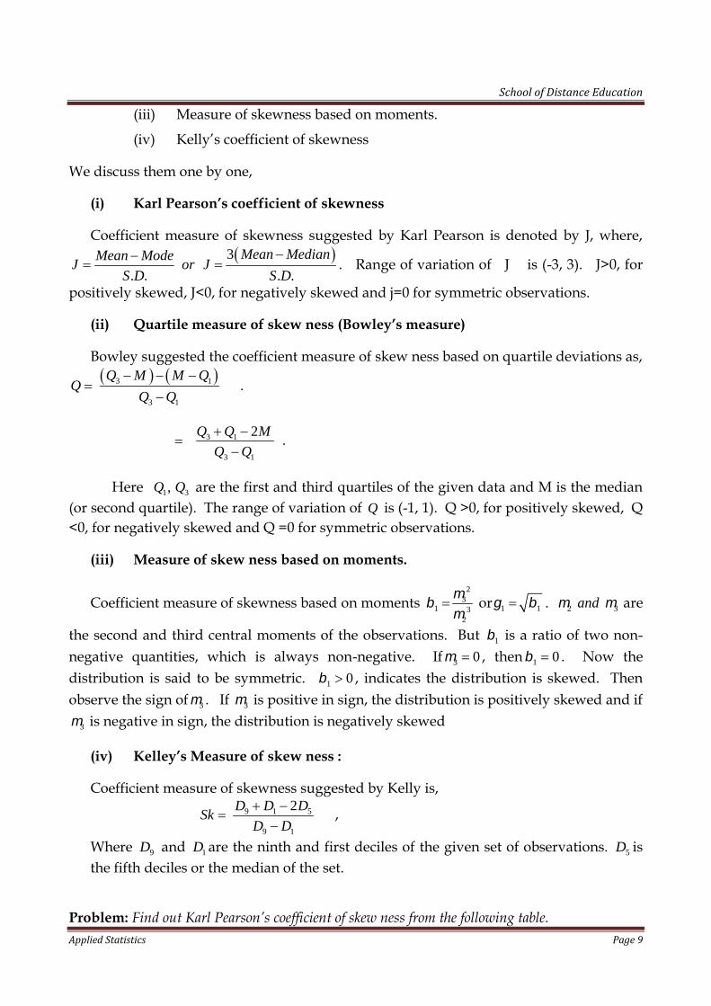
(iii) Measure of skewness based on moments.
(iv) Kelly’s coefficient of skewness
We discuss them one by one,
(i) Karl Pearson’s coefficient of skewness
Coefficient measure of skewness suggested by Karl Pearson is denoted by J, where, 3
. . . .
Mean MedianMean ModeJ or J
S D S D
. Range of variation of J is (-3, 3). J>0, for
positively skewed, J<0, for negatively skewed and j=0 for symmetric observations.
(ii) Quartile measure of skew ness (Bowley’s measure)
Bowley suggested the coefficient measure of skew ness based on quartile deviations as, 3 1
3 1
Q M M QQ
Q Q
.
3 1
3 1
2Q Q M
Q Q
.
Here 1 3,Q Q are the first and third quartiles of the given data and M is the median(or second quartile). The range of variation of Q is (-1, 1). Q >0, for positively skewed, Q<0, for negatively skewed and Q =0 for symmetric observations.
(iii) Measure of skew ness based on moments.
Coefficient measure of skewness based on moments2
31 3
2
or 1 1 . 2 3and are
the second and third central moments of the observations. But 1 is a ratio of two non-negative quantities, which is always non-negative. If 3 0 , then 1 0 . Now thedistribution is said to be symmetric. 1 0 , indicates the distribution is skewed. Thenobserve the sign of 3 . If 3 is positive in sign, the distribution is positively skewed and if
3 is negative in sign, the distribution is negatively skewed
(iv) Kelley’s Measure of skew ness :
Coefficient measure of skewness suggested by Kelly is,9 1 5
9 1
2D D DSk
D D
,
Where 9D and 1D are the ninth and first deciles of the given set of observations. 5D isthe fifth deciles or the median of the set.
Problem: Find out Karl Pearson’s coefficient of skew ness from the following table.

School of Distance Education
Applied Statistics Page 10
Wage: 0 – 10 10 – 20 20 – 30 30 – 40 40 – 50 50 – 60 60 – 70 70 – 80
No. of persons: 12 18 35 42 50 45 20 8
Solution:
Karl person’s coefficient o f skewness =. .
Mean ModeJ
S D
Mean, 1x f x
i iN i , Mode
1 0
1 0 1 2
c f fl
f f f f
Standard deviation= 2 21i i
i
f x xN
Necessary calculations follow:
frequency Mid-x fx 2fx
0 – 10
10 – 20
20 – 30
30 – 40
40 – 50
50 – 60
60 - 70
70 – 80
12
18
35
42
50
45
20
8
5
15
25
35
45
55
65
75
60
270
875
1470
2250
2475
1300
600
300
4050
21875
51450
101250
136125
84500
45000
230 9300 444550
Mean = 930040.43
230
S.D. = 2 21i i
i
f x xN
2
1 9300444550
230 230
= 17.27.
Here N=230, Maximum frequent class is 40 – 50; this is taken as the modal class.
Then, 0 42f , 1 50f and 2 45f
Hence, Mode
10 50 4240 46.15
50 42 50 45

School of Distance Education
Applied Statistics Page 11
Coefficient of skewness J 40.43 46.15
17.27
= - 0.3312.
Hence, the distribution is negatively skewed.
Problem: Calculate the quartile coefficient of skew ness for the following data:
x : 93 – 97 98 – 102 103 – 107 108 – 112 113 –117 118 – 122 123 – 127 128 - 132
f : 2 5 12 17 14 6 3 1
Solution:
Quartile coefficient of skew ness 3 1
3 1
2Q Q MQ
Q Q
Class adjusted Frequency L.T. Cum. freq.
92.5 –97.5
97.5 – 102.5
102.5 – 107.5
107.5 – 112.5
112.5 – 117.5
117.5 – 122.5
122.5 – 127.5
127.5 – 132.5
2
5
12
17
14
6
3
1
2
7
19
36
50
56
59
60
N=60
Class in which4
thN = 15th observation lies is 102.5 – 107.5
Class in which2
thN = 30th observation lies is 107.5 – 112.5
Class in which 3
4
thN = 45th observation lies is 112.5 – 117.5
Hence,1 1
1 11
4N
m cQ l
f
607 5
4102.5
12
= 105.83

School of Distance Education
Applied Statistics Page 12
3 3
3 33
34N
m cQ l
f
3 6036 5
4112.5
14
= 115.714
Median2 2
2 22
2N
m cQ l
f
6019 5
2107.5
17
= 110.735
Then 3 1
3 1
2Q Q MQ
Q Q
= 115.714 105.83 2 110.735
115.714 105.83
= 0.0075.
The distribution is slightly positively skewed.
Problem: First four moments about the value 5 of a distribution are 2, 20, 40 and 50. Calculatethe mean, variance, coefficient of skew ness and coefficient of kurtosis and comment on the nature ofthe distribution.
Solution:
Given, 1
'(5)1
15
k
ii
if xN
= 2 ; 21
'(5)2
15
k
ii
if xN
= 20;
1
3'(5)3
15
k
ii
if xN
= 40 and 1
4'(5)4
15
k
ii
if xN
= 50.
1
'(5)1
15 2
k
ii
if xN
2 5 7x
We have,
2
1 2' ' ' ' ' '( ) ( ) ( ) ( ) ( ) ..... 1 ( )
1 1 2 1 1r
rrr rA C A A C A A Ar r r
Hence2
2' '(5) (5)2 1
= 20 – 4 = 16
3
3' ' ' '(5) 3 (5) (5) 2 (5)3 2 1 1
340 - 3 20 2 + 2 2 = - 64

School of Distance Education
Applied Statistics Page 13
23
1 32
=
2
3
641
16
Since coefficient of skew ness is negative the distribution is negatively skewed.
1.4. Kurtosis:
The word kurtosis in Greek language means ‘bulginess’. Majority of the frequencycurves are bell shaped, more or less symmetric and unimodal. But the concentration ofobservations in the neighbourhood of mode may differ. If the frequency curve is almost
same in shape to the graph of the function2
21( ) ;
2
x
f x e x
, then the curve is
said to be a normal curve. The peaked ness or flatness of a frequency curve in comparisonwith normal curve is known as kurtosis. If more observations are concentrated in theneighbourhood of mode, the curve becomes more peaked than the normal curve and thedistribution is said to be lepto kurtic. Relatively less concentration of observations in theneighbourhood of mode makes the curve more flat than the normal curve. Then thedistribution is said to be platy kurtic. The distribution with frequency curve almost sameto the normal curve, it is said to be meso kurtic.
The shapes of different types of frequency curves are given here.
W.S. Gosset, humorously gives a narration on kurtosis as, “platykurtic curves, like theplatypus, are squat with short tails; leptokurtic curves are high with long tails like thekangaroos noted for leaping” and the sketch is as follows:
1.4.1. Measures of Kurtosis:
The measure of peak ness of flatness of the frequency distribution is the measure ofkurtosis. Following are the various measures of kurtosis.
(i) Measure of kurtosis based on moments.

School of Distance Education
Applied Statistics Page 14
Coefficient measure of kurtosis based on moments 42 2
2
or 2 2 3 . 4 2and
are the fourth and second central moment of the set of observations. 2 > 3 forleptokurtic. 2 =3, for meso kurtic and 2 < 3, for platy kurtic.
(ii) Measure of kurtosis based on quartiles.
Coefficient of kurtosis3 1
0.9 0.1
1( )
2Q Q
kQ Q
, where 3Q and 1Q are the first and third
quartiles. 0.9Q and 0.1Q are the observations which come at the 9
10
thN
and10
thN
position
when the observations are arranged in ascending order of magnitude or they are calledthe 9th and 1st deciles. For a meso kurtic distribution, k will be near about 0.25.
Problem: First four moments about the value 5 of a distribution are 2, 20, 40 and 50. Calculatethe mean, variance, coefficient of kurtosis and comment on the nature of the distribution.
Solution:
Given, 1
'(5)1
15
k
ii
if xN
= 2 ; 21
'(5)2
15
k
ii
if xN
= 20;
1
3'(5)3
15
k
ii
if xN
= 40 and 1
4'(5)4
15
k
ii
if xN
= 50.
1
'(5)1
15 2
k
ii
if xN
2 5 7x
We have,
2
1 2' ' ' ' ' '( ) ( ) ( ) ( ) ( ) ..... 1 ( )
1 1 2 1 1r
rrr rA C A A C A A Ar r r
Hence2
2' '(5) (5)2 1
= 20 – 4 = 16
3
3' ' ' '(5) 3 (5) (5) 2 (5)3 2 1 1
340 - 3 20 2 + 2 2 = - 64

School of Distance Education
Applied Statistics Page 15
2 4
4' ' ' ' ' '(5) 4 (5) (5) 6 (5) (5) 3 (5)4 3 1 2 1 1
= 2 450 - 4 40 2 + 6 20 2 - 3 2 = 162
42 2 2
2
1620.6328
16
Since the coefficient of kurtosis is less than 3, the distribution is platy kurtic.
Problem: Find the coefficient of kurtosis based on quartiles to the following data.
. Calculate the quartile coefficient of skew ness for the following data:
x : 10 – 15 16 – 20 21 – 25 26 – 30 31 – 35 36 – 40 41 – 45
f : 3 4 68 30 10 6 2
Solution:
Coefficient of kurtosis3 1
0.9 0.1
1( )
2Q Q
kQ Q
Class adjusted Frequency L.T. Cum. freq.
9.5 – 15.5
15.5 – 20.5
20.5 – 25.5
25.5 – 30.5
30.5 – 35.5
35.5 – 40.5
40.5 – 45.5
3
4
68
30
10
6
2
3
7
75
105
115
121
123
N=123
Class in which4
thN = 31st observation lies is 20.5 – 25.5

School of Distance Education
Applied Statistics Page 16
Class in which 3
4
thN = 93rd observation lies is 25.5 – 30.5
Class in which10
thN = 12th observation lies is 20.5 – 25.5
Class in which 9
10
thN = 111th observation lies is 30.5 – 35.5
Hence,1 1
1 11
4N
m cQ l
f
1237 5
420.5
68
= 22.25
3 3
3 33
34N
m cQ l
f
3 12375 5
425.5
30
= 28.375
0.1 0.1
0.1 0.10.1
10N
m cQ l
f
1237 5
1020.5
68
= 20.89
0.9 0.9
0.9 0.90.9
910N
m cQ l
f
9 123105 5
1030.5
10
= 33.35
Coefficient of kurtosis3 1
0.9 0.1
1( )
2Q Q
kQ Q
=
1(28.375 22.25)
233.35 20.89
= 0.2457
Since k is almost near to 0.25, the curve is almost meso kurtic.
EXERCISES
1. Define skewness. What are the measures of skewness?
2. Define kurtosis. Explain the various measures of kurtosis.
3. Calculate skew ness and kurtosis for the following distribution:
Class: 1 – 5 6 – 10 11 –15 16 – 20 21 – 25 26 - 30 31 –35
Frequency: 3 4 68 30 10 6 2
School of Distance Education
Applied Statistics Page 17
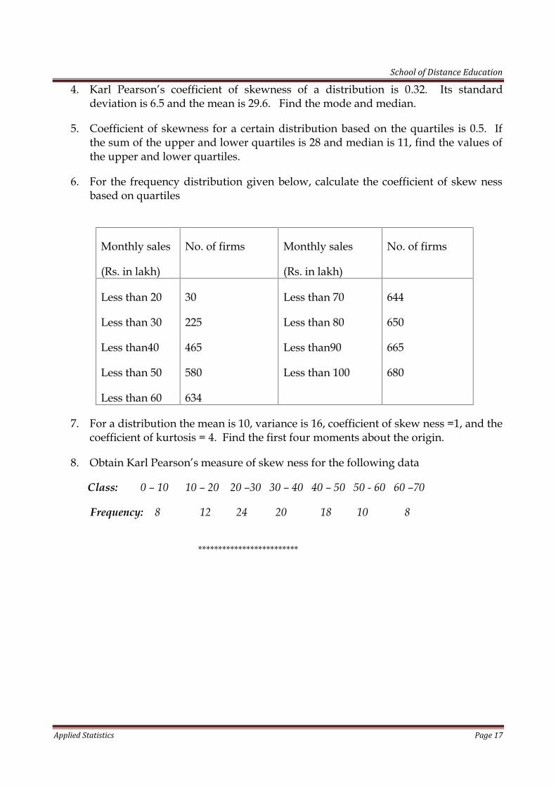
4. Karl Pearson’s coefficient of skewness of a distribution is 0.32. Its standarddeviation is 6.5 and the mean is 29.6. Find the mode and median.
5. Coefficient of skewness for a certain distribution based on the quartiles is 0.5. Ifthe sum of the upper and lower quartiles is 28 and median is 11, find the values ofthe upper and lower quartiles.
6. For the frequency distribution given below, calculate the coefficient of skew nessbased on quartiles
Monthly sales
(Rs. in lakh)
No. of firms Monthly sales
(Rs. in lakh)
No. of firms
Less than 20
Less than 30
Less than40
Less than 50
Less than 60
30
225
465
580
634
Less than 70
Less than 80
Less than90
Less than 100
644
650
665
680
7. For a distribution the mean is 10, variance is 16, coefficient of skew ness =1, and thecoefficient of kurtosis = 4. Find the first four moments about the origin.
8. Obtain Karl Pearson’s measure of skew ness for the following data
Class: 0 – 10 10 – 20 20 –30 30 – 40 40 – 50 50 - 60 60 –70
Frequency: 8 12 24 20 18 10 8
*************************

School of Distance Education
Applied Statistics Page 18
CHAPTER 2
CORRELATION AND REGRESSION
2.1. Introduction:
Let us consider two characteristics X and Y which are numerically measurable.Assume X denotes the height and Y denote corresponding weight of college students. Fora set of students, when we are recording their height (X) and weight (Y), we get twovalues for an individual. One value corresponds to the height and the other valuecorresponds to the weight of that individual. We record the data for that individual as anordered pair. The procedure repeats for all the students and finally we get a set ofordered pairs on X and Y. We call such a data on two characteristics as bivariate data. Toanalyze whether there is any relation between these characteristics, there are two distinctaspects for the study. One is correlation analysis and the other is regression analysis.Correlation analysis is to determine the degree of linear relationship between thecharacteristics X and Y. Regression analysis is to establish the nature of linear relationshipbetween the characteristics. A simple method to get a rough idea on correlation andregression of the two characteristics considered is scatter method.
2.2. Scatter Diagram:
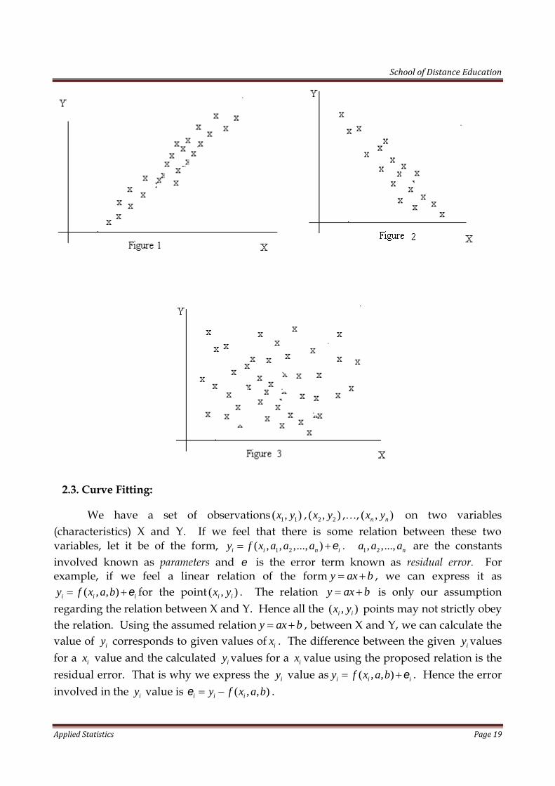
Let 1 1( , )x y , 2 2( , )x y ,…, ( , )n nx y be the set of observations obtained on the twocharacteristics X and Y. A diagram obtained by plotting these values 1 1( , )x y , 2 2( , )x y ,…,( , )n nx y , on a graph is called scatter diagram. It consists of points scattered over the graph.Consider the following scatter diagrams obtained by plotting the observations regardingto some X and Y.
In the first scatter diagram (figure 1), we can observe that all the points are almostscattered around a straight line. Also the line is of the form, as X increases Y alsoincreases. Then we can roughly say, there exist a positive linear relation between X and Y.Since the points are closely clustered around the straight line, there is a high degree oflinear relation.
In the second diagram (figure 2), also we observe that all the points are almostscattered around a straight line. But the line is of the form, as X increases Y decreases.Then we can suspect there exist a negative linear relation between X and Y. Here also, thepoints are closely clustered around the straight line. Hence the degree of linear relation ishigh.
In the next scatter diagram (figure 3), no specific relation between X and Y isobserved. Then one can infer that there is no correlation between X and Y.
School of Distance Education
Applied Statistics Page 19
2.3. Curve Fitting:
We have a set of observations 1 1( , )x y , 2 2( , )x y ,…, ( , )n nx y on two variables(characteristics) X and Y. If we feel that there is some relation between these twovariables, let it be of the form, 1 2( , , ,..., )i i n iy f x a a a . 1 2, ,..., na a a are the constantsinvolved known as parameters and is the error term known as residual error. Forexample, if we feel a linear relation of the form y ax b , we can express it as
( , , )i i iy f x a b for the point ( , )i ix y . The relation y ax b is only our assumptionregarding the relation between X and Y. Hence all the ( , )i ix y points may not strictly obeythe relation. Using the assumed relation y ax b , between X and Y, we can calculate thevalue of iy corresponds to given values of ix . The difference between the given iy valuesfor a ix value and the calculated iy values for a ix value using the proposed relation is theresidual error. That is why we express the iy value as ( , , )i i iy f x a b . Hence the errorinvolved in the iy value is ( , , )i i iy f x a b .

School of Distance Education
Applied Statistics Page 20
In general consider the relation between X and Y of the form,1 2( , , ,..., )i i n iy f x a a a . Then the residual error on iy value 1 2( , , ,..., )i i i ny f x a a a . To
identify the relation between X and Y in terms of the parameters 1 2, ,..., na a a , it is toestimate the values of these parameters. The best values of 1 2, ,..., na a a are those values of
1 2, ,..., na a a which makes the residual errors minimum. The process of determining thebest values of the parameters 1 2, ,..., na a a , statistically known as curve fitting. The values ofthe parameters are estimated using the Principle of least squares.
The Principle of least squares states that the best estimates of 1 2, ,..., na a a are those valuesof 1 2, ,..., na a a which minimize the sum of squares of the residual errors for all iy values.Then it is to find the values of 1 2, ,..., na a a which minimizing
2
21 2
1 1
( , , ,..., )n n
i i i ni i
E y f x a a a
.
The values of 1 2, ,..., na a a which minimizes E can be obtained by solving the
following equations,1
0E
a
,
2
0E
a
,…, 0
n
E
a
.
These equations are known as normal equations.
Fitting of a straight line y ax b
Consider 1 1( , )x y , 2 2( , )x y ,…, ( , )n nx y are the observations taken. It is to fit a maximumsuitable straight line for the given data. That is to estimate the best values of theparameters involved a and b. By the Principle of least squares, the best values of a and bare those values of a and b which minimizes E, where,
2 2
2
1 1 1
( , , ) ( )n n n
i i i i ii i i
E y f x a b y ax b
The normal equations are 0E
a
and 0
E
b
2
1
0 ( ) 0n
i ii
Ey ax b
a a
1
2 ( ) 0n
i i ii
y ax b x
2
1 1 1
(1)n n n
i i i ii i i
x y a x b x
School of Distance Education
Applied Statistics Page 21
2
1
0 ( ) 0n
i ii
Ey ax b
b b
1
1 ( ) 0n
i ii
y ax b
1 1
(2)n n
i ii i
y a x n b
Solving (1) and (2) using the given data, the best estimates of a and b can be obtained.
If the given X, Y values are big values, to make the calculations easy, transform X, Yvalues to U, V values in the form, make a transformation on X, Y values to reduce them
x au
b
and y c
vd
. Then fit a line of the form ' 'v a u b and hence re substitute u and
v to get the required relation in terms of X and Y.
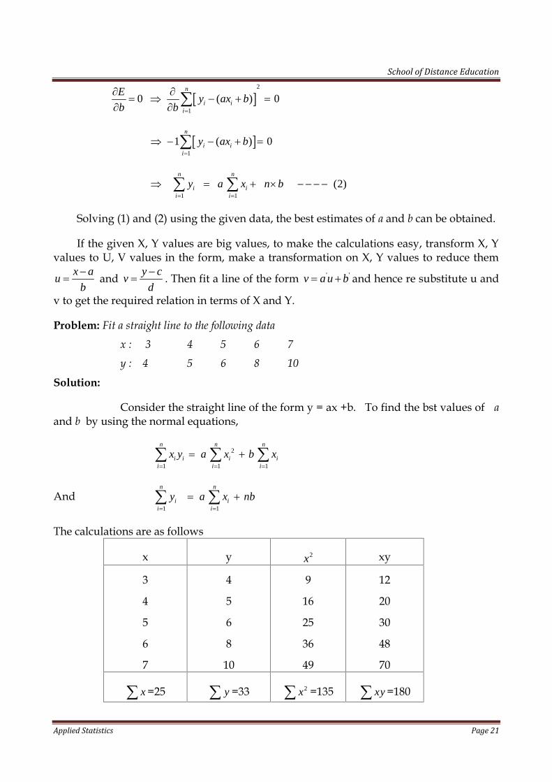
Problem: Fit a straight line to the following data
x : 3 4 5 6 7
y : 4 5 6 8 10
Solution:
Consider the straight line of the form y = ax +b. To find the bst values of aand b by using the normal equations,
2
1 1 1
n n n
i i i ii i i
x y a x b x
And1 1
n n
i ii i
y a x nb
The calculations are as follows
x y 2x xy
3
4
5
6
7
4
5
6
8
10
9
16
25
36
49
12
20
30
48
70
x =25 y =33 2x =135 xy =180
School of Distance Education
Applied Statistics Page 22
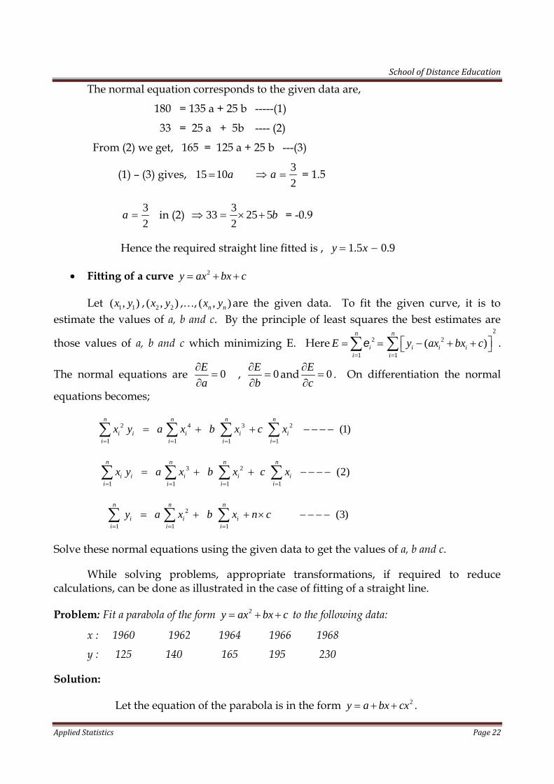
The normal equation corresponds to the given data are,
180 = 135 a + 25 b -----(1)
33 = 25 a + 5b ---- (2)
From (2) we get, 165 = 125 a + 25 b ---(3)
(1) – (3) gives, 15 10a3
2a = 1.5
3
2a in (2) 3
33 25 52
b = -0.9
Hence the required straight line fitted is , 1.5 0.9y x
Fitting of a curve 2y ax bx c
Let 1 1( , )x y , 2 2( , )x y ,…, ( , )n nx y are the given data. To fit the given curve, it is toestimate the values of a, b and c. By the principle of least squares the best estimates are
those values of a, b and c which minimizing E. Here2
2 2
1 1
( )n n
i i i ii i
E y ax bx c
.
The normal equations are 0E
a
, 0
E
b
and 0
E
c
. On differentiation the normal
equations becomes;
2 4 3 2
1 1 1 1
(1)n n n n
i i i i ii i i i
x y a x b x c x
3 2
1 1 1 1
(2)n n n n
i i i i ii i i i
x y a x b x c x
2
1 1 1
(3)n n n
i i ii i i
y a x b x n c
Solve these normal equations using the given data to get the values of a, b and c.
While solving problems, appropriate transformations, if required to reducecalculations, can be done as illustrated in the case of fitting of a straight line.
Problem: Fit a parabola of the form 2y ax bx c to the following data:
x : 1960 1962 1964 1966 1968
y : 125 140 165 195 230
Solution:
Let the equation of the parabola is in the form 2y a bx cx .

School of Distance Education
Applied Statistics Page 23
To identify the best values of a,b and c, we use the following normal equations
2 2 3 4
1 1 1 1
(1)n n n n
i i i i ii i i i
x y a x b x c x
2 3
1 1 1 1
(2)n n n n
i i i i ii i i i
x y a x b x c x
2
1 1 1
(3)n n n
i i ii i i
y na b x c x
But here the given values of the variables are huge numbers. So first we transformx and y to some new variable u and v then, fit a parabola for u and v. Using this, derivethe parabola for x and y. The working methods are shown below
x y u=1964
2
x v=165
5
y
2u 3u 4u uv 2u v
1960
1962
1964
1966
1968
125
140
165
195
230
-2
-1
0
1
2
-8
-5
0
6
13
4
1
0
1
4
-8
-1
0
1
8
16
1
0
1
16
16
5
0
6
26
-32
-1
0
6
52
0 6 10 0 34 53 25
The normal equations in terms of u and v are,
2 2 3 4
1 1 1 1
n n n n
i i i i ii i i i
u v a u b u c u
2 3
1 1 1 1
n n n n
i i i i ii i i i
u v a u b u c u
2
1 1 1
n n n
i i ii i i
v na b u c u
Corresponds to the given data, these normal equation are,
25 10 0 34 (1)a b c

School of Distance Education
Applied Statistics Page 24
53 0 10 0 (2)a b c
6 5 0 10 (3)a b c
53(2) 5.3
10b
13(1) 2(3) 13 14 0.929
14c c
Then, 5a = 6- 10(0.929) 0.658a
Now the parabola is, 20.658 5.3 0.929v u u
Substitute u and v as 1964
2
x and 165
5
y respectively,
We get,2
165 1964 19640.658 5.3 0.929
5 2 2
y x x
21964 3928 3857296165 3.29 26.5 4.645
2 4
x x xy
21.161 4547.15 4410689.85y x x
Fitting of a curve xy ab
Taking logarithm to the base 10 on both sides, the curve xy ab becomes,log log logy a x b . Let logY y , logA a and logB b . Now the required curve is ofthe form, Y A Bx orY B x A . If we are given x and Y values, it is easy to estimatethe parameters A and B, using the method of fitting a straight line. Hence we can obtain aand b as the antilogarithm of A and B respectively.
To fit a curve of the form xy ab for the given set of observations 1 1( , )x y , 2 2( , )x y ,…,( , )n nx y , get iY values by taking the logarithm of the given iy values. Using the i ix and Y
values, solve the following normal equations for estimating A and B,
2
1 1 1
(1)n n n
i i i ii i i
x Y B x A x
and
1 1
(2)n n
i ii i
Y B x nA
Solve (1) and (2) to obtain A and B, then by taking antilogarithm of A and B we get a andb. Hence the curve xy ab is fitted.

School of Distance Education
Applied Statistics Page 25
Fitting of a curve by ax
After taking logarithm on both sides the curve by ax also can be converted in theform of a straight line. That is, the curve becomes, log log logy a b x . Let logY y ;
logX x and logA a ; then the curve becomes, Y A bX orY bX A . Using the given
1 1( , )x y , 2 2( , )x y ,…, ( , )n nx y values, obtain i iX and Y values taking logarithm on i ix and y
values. Then solving the following normal equations A and b can be solved.
2
1 1 1
(1)n n n
i i i ii i i
X Y b X A X
and
1 1
(2)n n
i ii i
Y b X nA
The value of a is obtained by taking the antilogarithm of A. Hence the requiredcurve is fitted.
Fitting of a curve b xy ae
The method illustrated above can be used in the case of fitting of b xy ae also.Taking logarithm on both sides, the curve becomes, log log logy a x b e . Let logY y ;
logA a and logB b e , we get, Y A Bx orY Bx A . From the given 1 1( , )x y , 2 2( , )x y
,…, ( , )n nx y values, taking the logarithm of iy values iY values are obtained. Then use thefollowing normal equations to obtain A and B.
2
1 1 1
(1)n n n
i i i ii i i
x Y B x A x
and
1 1
(2)n n
i ii i
Y B x nA
Now, a is the antilogarithm of A andlog
Bb
e .
Problem: for the data given below, find the equation to he fitting exponential curve of the formbxy ae
x : 1 2 3 4 5 6
y : 1.6 4.5 13.8 40.2 125 300
Solution:

School of Distance Education
Applied Statistics Page 26
Taking logarithm to base 10 on both sides, the given curve bxy ae is in theform, log log logy a xb c
This is in the form, Y A Bx
where, logY y , logA a , logB b c
Using the values of Y and x, we can fit the line, Y A Bx , that is we can find bestvalues for A and B. Using these values of A and B, we can get the values of a and b.
For an easiness in calculation we transform x to u, where 3u x
Now using u and Y, fit a line of the form ' 'Y A B u , using the normal equations,
' 2 '
1 1 1
n n n
i i i ii i i
u Y B u A u
and
' '
1 1
n n
i ii i
Y B U nA
The calculations are as follows,
x y u=x-3 10logY y uY 2u
1
2
3
4
5
6
1.6
4.5
13.8
40.2
125
300
-2
-1
0
1
2
3
0.204
0.653
1.140
1.604
2.097
2.477
-0.408
-0.653
0
1.604
4.194
7.431
4
1
0
1
4
9
3 8.175 12.168 19
Here the normal equations for u and Y are
'12.168 3 19 'A B and ' '8.175 6 3A B
Solving these two equations we get, ' 1.13A and ' 0.46B
Hence the line connecting u and Y is 1.13 0.46Y u
That is 1.13 0.46 3Y x 0.25 0.46Y x
This implies, A = -0.25 and B = 0.46

School of Distance Education
Applied Statistics Page 27
That is 10log 0.25a and 10log 0.46b c
From here we get a = 0.557 and b = 1.06
Hence the required curve is,
1.060.557 xy e .
Problem: Fit a curve of the form by ax for the following data
x : 66 64 55 51 42 32 24
y : 2.5 7.5 12.5 17.5 25 40 75
Solution:
Taking logarithm on both sides of the required curve, by ax , we get,
log log logy a b x . This is in the form Y A bX , where logY y , logA a ,andlogX x .
The calculations are:
x y logX x logY y XY 2X
66
64
55
51
42
32
24
2.5
7.5
12.5
17.5
25
40
75
1.8195
1.8061
1.7403
1.7075
1.6232
1.5051
1.3802
0.3979
0.8751
1.0969
1.2430
1.3979
1.6021
1.8750
0.7239
1.5805
1.9089
2.1224
2.2690
2.4113
2.5879
3.3106
3.2619
3.0286
2.9156
2.6347
2.2653
1.9049
X =11.5819 Y =8.4879 XY=13.6036
2X =19.3216
The normal equations for Y A bX are,
2
1 1 1
n n n
i i i ii i i
X Y b X A X
, and
1 1
n n
i ii i
Y b X nA
Here the normal equations are,

School of Distance Education
Applied Statistics Page 28
13.6036 = 19.3216 b + 11.5819 A ---- (1)
8.4879 = 11.5819 b + 7 A ----- (2)
Solving these normal equations, we get, b = -2.773 and A = 5.8008
From A = 0.48, we get a = Anti log (A) = Anti log(5.8008) = 632120.68
Hence the required curve is ,
2.773632120.68y x .
Problem: Fit a curve of the form xy ab for the following data
x : 2 3 4 5 6
y : 144 172.8 207.4 248.8 298.6
Solution:
Taking logarithm on both sides of the required curve, xy ab , we getlog log logy a x b . This is in the formY A B x , where logY y , logA a , and logB b.
Using the values of logY y and x , we can find the best values of A and B usingthe normal equations for fitting the line Y A B x . From this the value of a and b canbe solved.
The calculations are:
x y logY y xY 2x
2
3
4
5
6
144
172.8
207.4
248.8
298.6
2.16
2.24
2.32
2.40
2.47
4.32
6.72
9.28
12
14.82
4
9
16
25
36
x =20 Y =11.59 xY =47.14 2x =90
The normal equations for Y A bX are,
2
1 1 1
n n n
i i i ii i i
x Y B x A x
, and1 1
n n
i ii i
Y B x nA
School of Distance Education
Applied Statistics Page 29
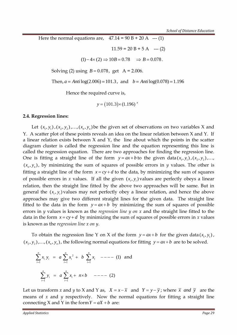
Here the normal equations are, 47.14 = 90 B + 20 A --- (1)
11.59 = 20 B + 5 A --- (2)
(1) 4 (2) 10 0.78B 0.078B .
Solving (2) using 0.078B , get A = 2.006.
Then, log(2.006) 101.3a Anti , and log(0.078) 1.196b Anti
Hence the required curve is,
101.3 (1.196) xy
2.4. Regression lines:
Let 1 1( , )x y , 2 2( , )x y ,…, ( , )n nx y be the given set of observations on two variables X andY. A scatter plot of these points reveals an idea on the linear relation between X and Y. Ifa linear relation exists between X and Y, the line about which the points in the scatterdiagram cluster is called the regression line and the equation representing this line iscalled the regression equation. There are two approaches for finding the regression line.One is fitting a straight line of the form y ax b to the given data 1 1( , )x y , 2 2( , )x y ,…,( , )n nx y , by minimizing the sum of squares of possible errors in y values. The other isfitting a straight line of the form x cy d to the data, by minimizing the sum of squaresof possible errors in x values. If all the given ( , )i ix y values are perfectly obeys a linearrelation, then the straight line fitted by the above two approaches will be same. But ingeneral the ( , )i ix y values may not perfectly obey a linear relation, and hence the aboveapproaches may give two different straight lines for the given data. The straight linefitted to the data in the form y ax b by minimizing the sum of squares of possibleerrors in y values is known as the regression line y on x and the straight line fitted to thedata in the form x cy d by minimizing the sum of squares of possible errors in x valuesis known as the regression line x on y.
To obtain the regression line Y on X of the form y ax b for the given data 1 1( , )x y ,
2 2( , )x y ,…, ( , )n nx y , the following normal equations for fitting y ax b are to be solved.
2
1 1 1
(1)n n n
i i i ii i i
x y a x b x
and
1 1
(2)n n
i ii i
y a x n b
Let us transform x and y to X and Y as, X x x and Y y y ; where x and y are themeans of x and y respectively. Now the normal equations for fitting a straight lineconnecting X and Y in the formY aX b are:

School of Distance Education
Applied Statistics Page 30
2
1 1 1
1 1
(3)
(4)
n n n
i i i ii i i
n n
i ii i
X Y a X b X and
Y a X n b
But here,1 1
( ) 0n n
i ii i
X x x
and1 1
( ) 0n n
i ii i
Y y y
Hence,
2
1 1
(3) 0n n
i i ii i
X Y a X b
1 1
22
1 1
n n
i i i ii i
n n
i ii i
X Y x x y ya
X x x
1
2
1
1
1
n
i ii
n
ii
x x y yn
x xn
That is ( , )
var( )
Cov x ya
x
(4) 0 0 0a n b b .
Then, the straight line is, ( , )0
var( )
Cov x yY X
x .
Hence the regression line y on x is, ( , )
var( )
Cov x yy y x x
x .
In as similar way, the regression line x on y is derived as,
( , )
var( )
Cov x yx x y y
y
In the regression line y on x, the coefficient of x,2
( , )
var( )xy
x
PCov x y
x is known as the
regression coefficient of y on x, denoted by yxb and in the regression line x on y, the
coefficient of y,2
( , )
var( )xy
y
PCov x y
y is known as the regression coefficient of x on y, denoted by
xyb .
The regression line y on x help us to predict the value of y for a given value of x,and the regression line x on y helps to predict the value of x for a given value of y.
School of Distance Education
Applied Statistics Page 31
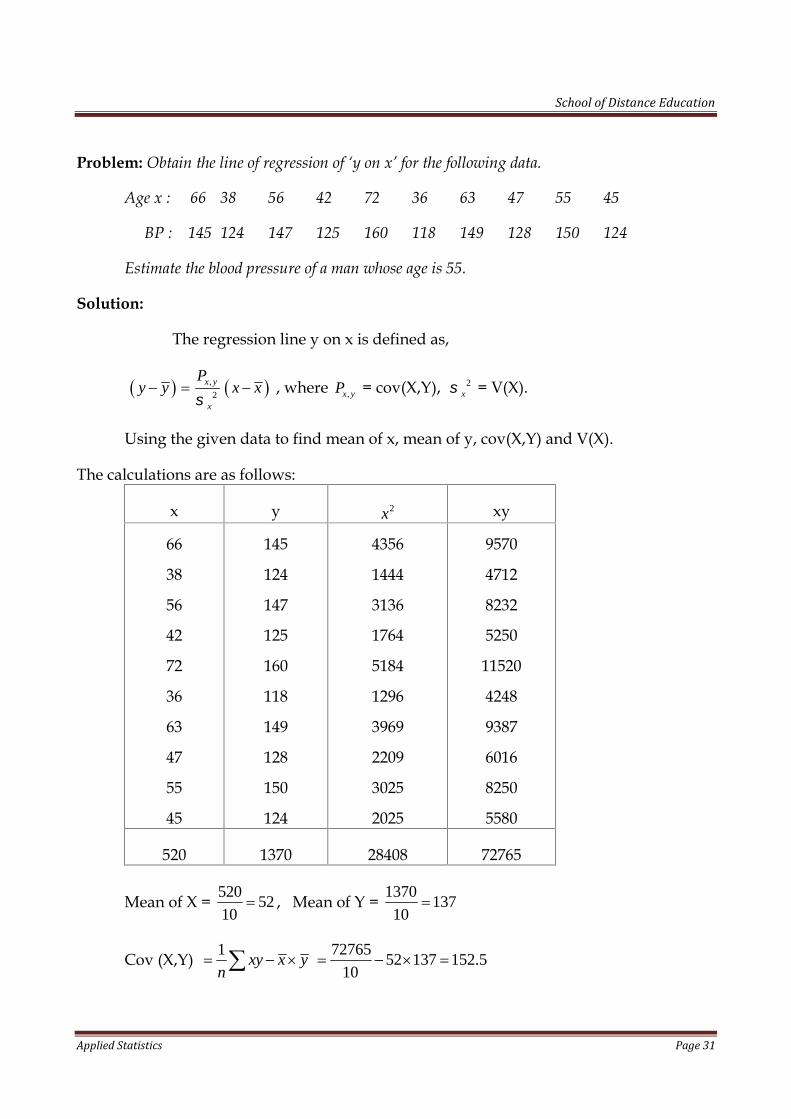
Problem: Obtain the line of regression of ‘y on x’ for the following data.
Age x : 66 38 56 42 72 36 63 47 55 45
BP : 145 124 147 125 160 118 149 128 150 124
Estimate the blood pressure of a man whose age is 55.
Solution:
The regression line y on x is defined as,
,
2
x y
x
Py y x x
, where ,x yP = cov(X,Y), 2
x = V(X).
Using the given data to find mean of x, mean of y, cov(X,Y) and V(X).
The calculations are as follows:
x y 2x xy
66
38
56
42
72
36
63
47
55
45
145
124
147
125
160
118
149
128
150
124
4356
1444
3136
1764
5184
1296
3969
2209
3025
2025
9570
4712
8232
5250
11520
4248
9387
6016
8250
5580
520 1370 28408 72765
Mean of X = 52052
10 , Mean of Y = 1370
13710
Cov (X,Y) 1xy x y
n 72765
52 137 152.510

School of Distance Education
Applied Statistics Page 32
2 21( )V X x x
n 228408
52 136.810
Hence the regression line of y on x is,
152.5137 52
136.8y x 1.1148 79.03y x
Then the blood pressure of a man whose age x = 55 can be get by substituting x =55 in the derived regression equation y on x, This implies, the blood pressure,
1.1148 55 79.03 140.34y .
Problem: For 10 observations on X and Y, the following data were observed
2 2130 , 200 , 2288 , 5506 , 3467x y x y xy
Obtain regression line of Y on X. Find y when x = 16.
Solution:
The regression line y on x is, ,
2
x y
x
Py y x x
, where ,x yP = cov(X,Y), 2
x = V(X)
1( , )Cov X Y xy x y
n
1 130 2003467
10 10 10
= 86.7
2
2 21 1 130( ) 2288
10 10V X x x
n
= 59.8
The regression line Y on X is, 200 86.7 130
10 59.8 10y x
1.4498 1.1526y x .
When x = 16, we get,
1.4498 16 1.1526 24.3494y .
2.5. Pearson’s Coefficient of correlation:
If there is a linear relation between the variables x and y, the degree of linearrelation is measured by the coefficient of correlation. If all they given ( , )i ix y points arealmost satisfying a linear relation, then we are saying that there is a high degree of linearrelation between the variables. If the linear relation fitted for the variables is in such a

School of Distance Education
Applied Statistics Page 33
way that the increment in one variable results in the increment of the other also, thenthere is a direct (or positive) correlation existing between the variables. On the otherhand, if the linear relation fitted for the variables is in such a way that the increment inone variable results in the decrease of the other, and then there is an inverse (or negative)correlation existing between the variables. If there is no linear relation existing betweenthe variables, the correlation is zero.
A famous British Statistician, Karl Pearson suggested a coefficient measure of thedegree of correlation between two variables x and y, known as Pearson’s coefficient ofcorrelation is denoted by xyr , where,
1
2 2
1 1
1( )( )
1 1( ) ( )
n
i ixy i
n n
i ii i
xyx y
x x y yP n
r
x x y yn n
1
2 2 2 2
1 1
1
1 1( ) ( )
n
i ii
n n
i ii i
x y xyn
x x y yn n
Theorem: For two variable x and y, 1 1xyr , where xyr is the Pearson’s coefficient ofcorrelation.
Proof:
Let 1 1( , )x y , 2 2( , )x y ,…, ( , )n nx y are the observations on x and y. Consider ( )i
x
x x
and
( )i
y
y y
, where x and y are the means and x and y are the standard deviations of x
and y respectively.
We have,2
( ) ( )0i i
x y
x x y y
, because it is the square of a real number.
Adding all such terms for i=1,2,…,n and dividing by n,
2( ) ( )1
0i i
i x y
x x y y
n
On expansion,2 2
2 2
( ) ( ) ( ) ( )1 1 12 0i i i i
i i ix y x y
x x y y x x y y
n n n
2 22 2
1 1 1 1 1 1( ) ( ) 2 ( )( ) 0i i i i
i i ix y x y
x x y y x x y yn n n

School of Distance Education
Applied Statistics Page 34
22
2 2
( , )2 0yx
x y x y
Cov x y
. That is, 1 1 2 0xy
x y
P
2 2 0xyr . That is, 1 0xyr
This gives, 1 0 1 0xy xyr or r
That is, 1 1xy xyr or r
1 1xyr
Remark: We have the regression coefficients y on x,2
xy
xyx
Pb
and the regression
coefficients x on y,2
xy
yxy
Pb
. The geometric mean of these regression coefficients gives
the magnitude of the coefficient of correlation xyr . The sign of correlation is determined bythe sign of covariance between x and y, xyP . If xyP is positive xyr is positive in sign and if
xyP is negative xyr is negative in sign.
Theorem: (Invariance of correlation coefficient under linear transformation): A
transformation on the variables x and y to u and v in the form x Au
c
and y B
vd
is
making no change in the coefficient of correlation between the variables. That is, xy uvr r
.
Proof:
Let 1 1( , )x y , 2 2( , )x y ,…, ( , )n nx y are the observations on x and y.
Then, 1
2 2
1 1
1( )( )
1 1( ) ( )
n
i ii
n n
i ii i
xy
x x y yn
r
x x y yn n
Let, x Au
c
and y B
vd
;
Then, Pearson’s coefficient of correlation between u and v,
1
2 2
1 1
1( )( )
1 1( ) ( )
n
i ii
n n
i ii i
uv
u u v vn
r
u u v vn n

School of Distance Education
Applied Statistics Page 35
1
2 2
1 1
1
1 1
ni i
i
n ni i
i i
uv
x A y Bx A y B
n c c d dr
x A y Bx A y B
n c c n d d
1
2 2
1 1
1
1 1
ni i
i
n ni i
i i
uv
x x y y
n c dr
x x y y
n c n d
1
2 2
1 1
1 1
1 1 1
n
i ii
n n
i ii i
uv
x x y ycd n
r
x x y ycd n n
1
1
xy
x y
uv
Pcdr
cd
xy
x y
P
uv xyr r .
Problem: Find the coefficient of correlation for the following data on X and Y.
X: 65 66 67 67 68 69 70 72
Y: 67 68 65 68 72 72 69 71
Solution:
Coefficient of correlation, xy
x yxy
Pr
To find x , y , xyP , 2x and 2
y
1
1 n
xy i ii
P x y xyn
; 2x = 2 2
1
1( )
n
ii
x xn
and 2y = 2 2
1
1( )
n
ii
y yn
The calculations are as follows:
x y 2x 2y xy

School of Distance Education
Applied Statistics Page 36
65
66
67
67
68
69
70
72
67
68
65
68
72
72
69
71
4225
4356
4489
4489
4624
4761
4900
5184
4489
4624
4225
4624
5184
5184
4761
5041
4355
4488
4355
4556
4896
4968
4830
5112
544 552 37028 38132 37560
1ix x
n 1
5448 = 68 ; 1
iy yn 1
5528 = 69
1
1 n
xy i ii
P x y xyn
= 137560 68 69 3
8
2x = 2 2
1
1( )
n
ii
x xn
= 2137028 68 4.5
8
2y = 2 2
1
1( )
n
ii
y yn
= 2138132 69 5.5
8
Coefficient of correlation, xy
x yxy
Pr
30.603
4.5 5.5 .
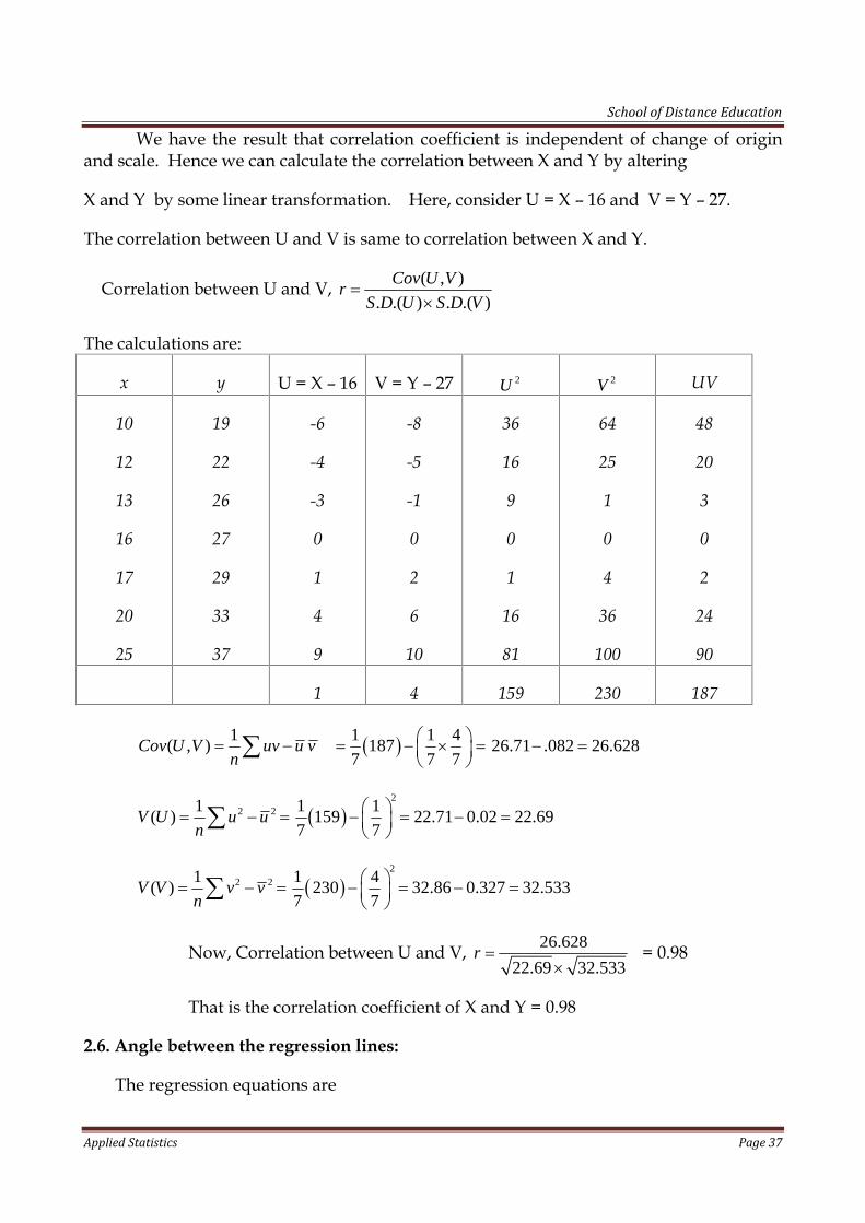
Problem: Calculate Karl Pearson’s coefficient of correlation for the following data;
x: 10 12 13 16 17 20 25
y: 19 22 26 27 29 33 37
Solution:
Coefficient of correlation ( , )
. .( ) . .( )
Cov X Yr
S D X S D Y
The problem can be solved by simply following the steps shown in above example.But for some computational easiness the problem can also be solved as in the followingillustration.
School of Distance Education
Applied Statistics Page 37
We have the result that correlation coefficient is independent of change of originand scale. Hence we can calculate the correlation between X and Y by altering
X and Y by some linear transformation. Here, consider U = X – 16 and V = Y – 27.
The correlation between U and V is same to correlation between X and Y.
Correlation between U and V, ( , )
. .( ) . .( )
Cov U Vr
S D U S D V
The calculations are:
x y U = X – 16 V = Y – 27 2U 2V UV
10
12
13
16
17
20
25
19
22
26
27
29
33
37
-6
-4
-3
0
1
4
9
-8
-5
-1
0
2
6
10
36
16
9
0
1
16
81
64
25
1
0
4
36
100
48
20
3
0
2
24
90
1 4 159 230 187
1( , )Cov U V uv u v
n 1 1 4
187 26.71 .082 26.6287 7 7
2
2 21 1 1( ) 159 22.71 0.02 22.69
7 7V U u u
n
2
2 21 1 4( ) 230 32.86 0.327 32.533
7 7V V v v
n
Now, Correlation between U and V, 26.628
22.69 32.533r
= 0.98
That is the correlation coefficient of X and Y = 0.98
2.6. Angle between the regression lines:
The regression equations are

School of Distance Education
Applied Statistics Page 38
2
xy
x
Py y x x
and
2
xy
y
Px x y y
Since xy
x yxy
Pr
, the regression coefficient y on x,
2
xy yxy
x x
Pr
and
The regression coefficient x on y,2
xy xxy
y y
Pr
.
Hence the regression equations are, yxy
x
y y r x x
---- (1) and
xxy
y
x x r y y
---- (2)
The regression equation x on y can be rewrite as y
xy x
y y x xr
---- (3)
Now the regression equation y on x [equation (1)] and that on x on y [equation (3)] can bewritten in the form y = m x + c as follows:
y yxy xy
x x
y r x r x y
---- (1) and
y y
xy yx xy yx
y x x yr r
---- (3)
From here, we get the slopes of these two regression lines as, 1y
xyx
m r
and 2
y
xy x
mr
Let us consider as the angle between the regression lines. Then,
1 2
1 2
tan1
1
y yxy
x xy x
y yxy
x xy x
rrm m
m mr
r
2
2 2
2 22
21
xy y y
xy x xy y y x
xy x x yy
x
r
r r
r

School of Distance Education
Applied Statistics Page 39
2 2
2 2
1tan xy y x
xy x x y
r
r
2
2 2
1tan xy x y
xy x y
r
r
Remarks:
(i) For two variables x and y, if 1xyr , we get tan 0 . This implies the angle betweenthe regression lines 1tan 0 0 . That is, if there is a perfect linear relation existsbetween x and y (whether it is direct or inverse), the angle between the regression line iszero. Or in other words, the two regression lines coincide or they are same.
(ii) If 0xyr , we get tan . This implies the angle between the regression lines1 0tan 90 . That is, if there is no linear relation exists between x and y, the two
regression lines are perpendicular.
If there are two regression lines, it is obvious that they are intersecting at a point. Thepoint of intersection of regression lines can be obtained by solving the regressionequations for x an y. It can be done as follows:
We have regression equation y on x; yxy
x
y y r x x
--- (1) and the regression
equation x on y; xxy
y
x x r y y
---- (2)
Put (2) in (1) gives, y xxy xy
x y
y y r r y y
2xyy y r y y
2 21 1xy xyr y r y y y
Put y y in (2) 0x x x x
Hence the point of intersection of the regression lines is ,x y
2.7. Identification of regression lines and determination of correlation coefficient
If we are given 1 1 1 0a x b y c and 2 2 2 0a x b y c as the two regression lines, it isto identify which of them represent regression line yon x and which is regression line x ony. For this first of all we assume the first line 1 1 1 0a x b y c is regression line y on x orregression line x on y. Let us assume the first line is regression line y on x. Then we
School of Distance Education
Applied Statistics Page 40
express the line in terms of y as, 1 1
1 1
a cy x
b b . Then the regression coefficient y on x is
1
1yx
ab
b . If the first line is assumed as regression line y on x the second is regression line
x on y. It is written in terms of x as, 2 2
2 2
b cx y
a a . If so, the regression coefficient x on y,
2
2xy
bb
a .
We know the geometric mean of regression coefficients is the magnitude ofcoefficient of correlation xyr and 1 1xyr .
Hence, if 1 2
1 2
1yx xy
a bb b
b a , we can confirm that our assumption regarding the
regression lines are same. Otherwise the first line is the regression line x on y and the
second is the regression line y on x. Then the regression coefficients are 1
1xy
bb
a and
2
2yx
ab
b . Then the coefficient of correlation, xyr 2 1
2 1
a b
b a , which is the reciprocal of xyr ,
obtained by previous assumption.
Problem: The two regression lines are5 6 90 0x y
15 8 130 0x y
Find (i) x , y (ii) regression coefficient of y on x and x on y (iii) correlation coefficient.
Solution:
Solving the given two regression lines,
5 6 90 0x y ----- (1) and 15 8 130 0x y ----- (2) , we get x , y .
(2) 3 (1) 10 400 40.y y
40, (1) 5 6 40 90 0 30.y in x x
, 30,40 .x y
Assume the first line is the regression line Y on X, then, the line can be expressed
as, 5 90
6 6y x . This implies the regression coefficient Y on X 1
1
5
6
a
b
. The second
School of Distance Education
Applied Statistics Page 41
line, X ion Y, can be expressed as, 8 130
15 15x y .Hence the regression coefficient X on
Y 2
2
8
15
b
a
.
Then, 1 2
2 1
a b
a b= 1 2
1 2
a b
b a
5 80.444 1
6 15
Hence our assumption is true. That is 5 6 90 0x y is regression line Y on Xand 15 8 130 0x y is the regression line X on Y. Then the regression coefficient of Y
on X = 5
6= 0.833. Regression coefficient of X on Y = 8
15= 0.533 and correlation
coefficient = 0.444. ( here the regression coefficients are positive)
Problem: Given that 14 12 3 0x y and 12 21 10 0x y are the regression lines for Xand Y. Identify the regression lines and find the correlation coefficient.
Solution:
Assume the 14 12 3 0x y is the regression line Y on X, then, 14 3
12 2y x .
This implies the regression coefficient Y on X 1
1
14
12
a
b
. The line
12 21 10 0x y is assumed as the regression line X on Y, then, 21 10
12 12x y . Then
the regression coefficient X on Y 2
2
21
12
b
a
.
Then, 1 2
2 1
a b
a b1 2
1 2
a b
b a
= 14 21
12 12 = 2.04 > 1. Hence our assumptions about the
regression lines are NOT true.
Now, 12 21 10 0x y is the regression line Y on X and the line14 12 3 0x y is the regression line X on Y .
Then, 12 10
21 21y x , and regression coefficient Y on X 1
1
12
21
a
b
.
And, 12 3
14 14x x , the regression coefficient X on Y 2
2
12
14
b
a
.

School of Distance Education
Applied Statistics Page 42
Then,, 1 2
2 1
a b
a b= 12 12
21 14 = 0.4898.
Since the regression coefficients are negative, the correlation coefficient is (- 0.4898).
Problem: The regression lines are y ax b and x cy d . If the two variables are having thesame mean, show that (1 ) (1 )d a b c .
Solution:
The means of x and y are obtained by solving the regression lines for x and y.
Here the first line is y ax b --(1) and the second is x cy d --(2) that is 1 dy x
c c --(3)
1(3) (1)
dand ax b x
c c
1/
1
d bc dx b a
c c ac
(1)1 1
bc d ad by a b
ac ac
This implies,1 1
bc d ad bx and y
ac ac
.
If the means of the variables are equal, we can write,1 1
bc d ad b
ac ac
This gives, bc d ad b d ad b bc
1 1a d b c .
Problem: If the variables x and y are satisfying the relation 0ax by c . Show that thecorrelation between x and y is -1 or +1, according as a and b are of the same sign or not.
Solution:
Since the variables are satisfying the relation 0ax by c , we can write this
relation in the line of the form y on x as, a cy x
b b ; and in the line of the form x on y as,
b cx y
a a . Then the regression coefficients y on x and x on y are identified as a
b , and
b
a respectively. Then the magnitude of the coefficient of correlation is obtained by the
geometric mean of the regression coefficients as, 1a b
b a . Then the correlation
coefficient can be +1 or -1 according as the regression coefficients are positive or negative.

School of Distance Education
Applied Statistics Page 43
The regression coefficients a
b and b
a becomes positive, when a and b are with
different signs. And they will become negative, when a and b are of same sign. Hence,the coefficient of correlation is -1 or +1, according as a and b are of the same sign or not.
2.8. Rank correlation coefficient
When we are considering two characteristics which are qualitative in nature, they arenot possible to measure numerically. For example consider the characteristics of theability in drawing (let it be X) and the ability in music (let it be Y). It is not possible tomeasure numerically the values of X and Y, for an individual. But if there are nindividuals, it is possible to rank these n individuals according to the ability in drawing(X) and according to their ability in music (Y). If these two characteristics are having highpositive correlation, then ranks obtained for the individuals based of X and Y will be insame order. If these two characteristics are having high negative correlation, then ranksobtained for the individuals based of X and Y will be in reverse order. Using the ranksobtained for the n individuals based on the characteristics X and Y, a method of findingthe coefficient of correlation is derived by C.Spearman in 1904. The coefficient ofcorrelation for two characteristics which are calculated based on the ranks is known asSpearman’s Rank Correlation Coefficient.
Let there be n individuals ranked according to two qualitative characteristicsconsidered. Let ( , )i ix y denote the rank of the thi individual when ranked according to thecharacteristics. So the ,i ix y values are the numbers from 1 to n.
Since ix values are the numbers from 1 to n, the mean of x values,1 ( 1) ( 1)
2 2
sum of first n natural numbers n n nx
n n
Similarly,1 ( 1) ( 1)
2 2
sum of first n natural numbers n n ny
n n
Variance of ix values,2
2 ( 1)
2x
sum of squares of first n natural numbers n
n
2
2
2
1 ( 1)(2 1) ( 1)
6 2
1
12
x
n n n n
n
n
;
Similarly,2
2 1
12y
n
.
Let i i id x y . This gives, 0d x y

School of Distance Education
Applied Statistics Page 44
Variance of ‘d’ values,
2 222 2
1 1
2
1
2
1
1 10
1
1
n n
d i i ii i
n
i ii
n
ii
d d x yn n
x yn
dn
Since x y , we can re write 2
1
1 n
ii
dn as, 22
1 1
1 1n n
i i ii i
d x x y yn n
2
2
1 1
1 1n n
i i ii i
d x x y yn n
2 2
2
1 1 1 1
1 1 1 12
n n n n
i i i i ii i i i
d x x y y x x y yn n n n
2 2 2
1
12cov( , )
n
i x yi
d x yn
But, we have, cov( , ) x yx y r , where r is the coefficient of correlation. Hence,
2 2 2
1
12
n
i x y x yi
d rn
Since,2
2 2 1
12x y
n
,
we get,2 2 2 2
2
1
1 1 1 1 12
12 12 12 12
n
ii
n n n nd r
n
2 22
1
1 1 12 2
12 12
n
ii
n nd r
n
2
2
1
1 11
6
n
ii
nd r
n

School of Distance Education
Applied Statistics Page 45
2
12
2
12
61
1
61 .
1
n
ii
n
ii
dr or
n n
dthe coefficient of correlation r
n n
Problem: The following are the ranks obtained by 10 students in Statistics and Mathematics
Statistics: 1 2 3 4 5 6 7 8 9 10
Mathematics: 1 4 2 5 3 9 7 10 6 8
To what extent is the knowledge of students in the two subjects related?
Solution:
Here to find the rank correlation coefficient of the ranks in Statistics andMathematics. Rank correlation coefficient is defined as,
2
2
61
( 1)
ii
dr
n n
, id is the difference in ranks.
The calculations are:
Rank inStat. ix Rank in Maths iy id = ix - iy 2id
1
2
3
4
5
6
7
8
9
10
1
4
2
5
3
9
7
10
6
8
0
-2
1
1
2
3
0
-2
3
2
0
4
1
1
4
9
0
4
9
4
36
Hence,
2
2
61
( 1)
ii
dr
n n
=
2
6 361 1 0.2189 0.7819
10(10 1)
Problem: 10 competitors in a music test were ranked by three judges A, B, and C in followingorder.

School of Distance Education
Applied Statistics Page 46
Ranks by A: 1 6 5 10 3 2 4 9 7 8
Ranks by B: 3 5 8 4 7 10 2 1 6 9
Ranks by C: 6 4 9 8 1 2 3 10 5 7
Discuss which pair of judges has the nearest approaches to common likings in music.
Solution:
Here to find the rank correlation coefficient between each pair of the judgesconsidering the ranks they given. Identify the pair of judges with high correlationcoefficient. They are considered having nearest approaches to common likings in music.
The calculations follow:
Ranksby A
ix
Ranksby B
iy
Ranksby C
iz
ix - iy ix - iz iy - iz 2i ix y 2i ix z 2i iy z
1
6
5
10
3
2
4
9
7
8
3
5
8
4
7
10
2
1
6
9
6
4
9
8
1
2
3
10
5
7
-2
1
-3
6
-4
-8
2
8
1
-1
-5
2
-4
2
2
0
1
-1
2
1
-3
1
-1
-4
6
8
-1
-9
1
2
4
1
9
36
16
64
4
64
1
1
25
4
16
4
4
0
1
1
4
1
9
1
1
16
36
64
1
81
1
4
200 60 214
Rank correlation between A and B,
2
2
61
( 1)
ii
dr
n n
=
2
6 2001 0.212
10(10 1)
Rank correlation between A and C,
2
2
61
( 1)
ii
dr
n n
=
2
6 601 0.6364
10(10 1)
Rank correlation between B and C,
2
2
61
( 1)
ii
dr
n n
=
2
6 2141 0.297
10(10 1)
It can be observed that the judges A and C are having nearest approaches tocommon likings in music.

School of Distance Education
Applied Statistics Page 47
Problem: Find the rank correlation coefficient for the following data:
X: 92 89 87 86 84 77 71 63 53 50
Y: 86 83 91 77 68 85 52 82 37 57
Solution:
First, the given values of X and Y should be ranked. If an observation repeats, thenthe sum of the ranks is equally divided among the observations. (For eg., when we areranking the observations in order, and let a number, say a, coming in the 6th and 7th
position then the first and second a values are assigned with the rank 6.5).
Here the observations are ranked in descending order. Then find the rankcorrelation coefficient.
x y Rank of X, ix Rank of Y, iy ix - iy 2i ix y
92
89
87
86
84
77
71
63
53
50
86
83
91
77
68
85
52
82
37
57
1
2
3
4
5
6
7
8
9
10
2
4
1
6
7
3
9
5
10
8
-1
-2
2
-2
-2
3
-2
3
-1
2
1
4
4
4
4
9
4
9
1
4
44
Rank correlation coefficient,
2
2
61
( 1)
ii
dr
n n
2
6 441 0.733
10(10 1)

School of Distance Education
Applied Statistics Page 48
Rank correlation coefficient when equal ranks (Tied ranks):
It may be noted that the Spearman’s rank correlation formula is derived on theassumption that all the ranks are different. But in practice, there are many situations,where more than one individual are getting the same rank. In a competition consider,three individuals received 3rd rank. They would have given the 3rd ,4th, and 5th rank, ifthere were slight difference in the evaluation. Then we add 3,4 and 5, which is 12. Then12 is equally divided for these three individuals. Hence we assign the rank 4 to each ofthese three individual. In such situations it is more accurate to calculate the Pearson’scoefficient of correlation between the ranks directly after assigning the average rank tothose with the same rank. But there is also a modified formula of Spearman’s rankcorrelation coefficient, which is as follows:
2 2 2
1
2
1 16 1 1
12 121
1
n
i i i j ji i j
d m m m m
rn n
, where, im stands for the number of
times the thi rank repeats in the x series of ranks and jm is the number of times the thj rankrepeats in the y series of ranks when the average ranks are assigned. The method isillustrated below:
Obtain the rank correlation coefficient for the following data:
X: 15 20 28 12 40 60 20 80
Y: 40 30 50 30 20 10 30 60
Illustration:
At first we assign ranks for X and Y values. Here we have 8 sets of data. That isn=8.
The ranks are:
X: 7 5.5 4 8 3 2 5.5 1
Y: 3 5 2 5 7 8 5 1
Here in X values, 20 repeats twice, with the possible ranks, 5 and 6. Hence itsaverage 5.5 is supplied for the value 20. Similarly in Y values, 30 repeat thrice, withpossible ranks 4, 5 and 6. Hence their average 5 is assigned as the ranks of the values 30.Now the difference in ranks, i i id X Y values are:
id : 4 0.5 2 3 -4 -6 0.5 0
2id : 16 0.25 4 9 16 36 0.25 0

School of Distance Education
Applied Statistics Page 49
This gives, 2 81.50ii
d .
2im (Because on X values, only the value 20 repeats twice) and 3jm ( because on Yvalues, only the value 30 repeats thrice).
Hence,
2 2 2
1
2
1 16 1 1
12 121
1
n
i i i j ji i j
d m m m m
rn n
2 2
2
1 16 81.50 2 2 1 3 3 1
12 121
8 8 1
6 81.50 0.5 21
8 63
= 0.
2.9. Partial and Multiple Correlations:
In a statistical study, if there are many variables included, and whenever we areinterested in studying the joint effect of a group of variables upon a variable not includedin that group, our study is on multiple correlations and multiple regressions.
For eg., in the study on the yield of a crop per acre (let it be 1X ), the value of thevariable 1X , is a joint effect of the variables, quality of seed 2X , fertility of soil 3X
,fertilizer used 4X , irrigation facilities 5X , whether conditions 6X and so on.
If we are considering the relation between two variables only, there are twoalternatives;
(i) We consider only those two members of the observed data in which theother members have specified values. Or,
(ii) We may eliminate mathematically the effect of other variables on the twovariables under consideration.
[The first method has the disadvantage that it limits the size of the data and also it willapplicable only the data in which the other variables have assigned values]
In second method it may not possible to eliminate the entire influence of the variables, butthe linear effect can easily eliminated. The correlation and regression between only twovariables eliminating the linear effects of other variables in considered is called the partialcorrelation and partial regression.
Let us limit our discussion with three variables 1X , 2X and 3X .

School of Distance Education
Applied Statistics Page 50
The equation of plane of regression of 1X on 2X and 3X is,
1 12.3 2 13.2 3 (1)X a b X b X
Let the observations on 1X , 2X and 3X are measured from their respective means, ie., 1 1 1iX x x , 2 2 2iX x x and 3 3 3iX x x .
Then, 1 1 2 2 3 3 0i i ix x x x x x . That is 1 2 3 0X X X
Taking summation on (1), we get a=0.
Then (1) implies, 1 12.3 2 13.2 3 (2)X b X b X
The coefficients 12.3b and 13.2b are the partial regression coefficients of 1X on 2X andthat of 1X on 3X respectively.
12.3 12.3 2 13.2 3e b X b X is called the estimate of 1X as given by the equation of planeof regression (2).
The quantity 1.23 1 12.3 2 13.2 3X X b X b X is called the error estimate or residual.
In the subscript of the residual 1.23X , the subscript before ‘.’ ie., 1 is known as theprimary subscript and the other after the subscript, ie, 2 and 3 are called the secondarysubscripts.
The order of regression coefficients are determined by the number of secondarysubscripts. For eg., 12.3b is the regression coefficient of order 1. In 12.3b , 2X is independentand 1X is dependent. In 21.3b , 1X is independent and 2X is dependent.
From the equation of plane of regression given in (2), the y the constants b’s aredetermined by the principle of least squares.
Sum of squares of residuals,
22
1.23 1 12.3 2 13.2 3S X X b X b X
2 1 12.3 2 13.2 312.3
0 2 0S
X X b X b Xb
3 1 12.3 2 13.2 313.2
0 2 0S
X X b X b Xb
2 1.23 0X X and 3 1.23 0X X
School of Distance Education
Applied Statistics Page 51
21 2 12.3 1 13.2 2 3
21 3 12.3 2 3 13.2 3
0(3)
0
X X b X b X X
X X b X X b X
Since 'iX s are measured from their respective means, we have, 2 21 1
1X
N ,
1cov( , )i j i jX X X X
N and
cov ,i j i j
i j i ji j
X X X Xr
N .
Hence, the equations given in (3), gives,
212 1 2 12.3 2 13.2 23 2 3
213 1 3 12.3 23 2 3 13.2 3
(4)r b b r
r b r b
12 1 12.3 2 13.2 23 3
13 1 12.3 23 2 13.2 3
(4) r b b r
r b r b
Solving these equations, we get,
12 1 23 3 12 23
13 1 3 13112.3
2 23 3 232
23 2 3 23
1
1
1
r r r r
r rb
r r
r r
and,
23 2 13 1 23 13
2 12 1 12113.2
23 2 3 233
2 23 3 23
12
23 131
233
23
1
1
1
1
1
1
r r r r
r rb
r r
r r
r
r r
r
r
If we write,12 13
21 23
31 32
1
1
1
r r
r r
r r
, and i j is the cofactor of the ( , )thi j element of , then,
1 1212.3
2 11
b
and 13113.2
3 11
b
. Now we get,
131 12 11 2 3
2 11 3 11
X X X

School of Distance Education
Applied Statistics Page 52
31 211 12 13
1 2 3
0XX X
.
2.10. Properties of residuals
(i) Sum of the product of any residual of order zero with any other residual ofhigher order is zero, provided the subscript of the former occurs among thesecondary subscripts of the later.
(ii) 21.2 1.23 1 1.23 1.23X X X X X
(iii) The sum of the product of two residuals is zero, if all the subscript (primaryas well as secondary) of the one occur among the secondary subscripts of theother. Eg., 1.2 3.12 0X X , 2.3 1.23 0X X
2.11. Coefficient of multiple correlations
Consider the variables 1X , 2X and 3X has N observations. The multiple correlationof 1X on 2X and 3X , usually denoted by 1.23R is the simple correlation coefficient between
1X and the joint effect of 2X and 3X on 1X . In other words, 1.23R is the correlationcoefficient between 1X and its estimated value as given by the plane of regression of 1X on
2X and 3X .
That is, 1 1.231.23
1 1.23
cov( , )
( ) ( )
X eR
V X V e , which is derived as,
2 22 12 13 12 13 231.23 2
23
2
1
r r r r rR
r
Multiple correlation coefficient measures the closeness of the association betweenthe observed values and expected values of a variable obtained from the multiple linearregression of that variable on the other variables. It is proved that 1.230 1R .
If 1.23 1R , then association is perfect and all the predicted value of 1X coincide withthe observed values of 1X .
If 1.23 0R , then 1X is completely uncorrelated with the predicted values of 1X .That is the regression equation fails to throw any light on the value of 1X , when 2X and
3X are known.
2.12. Coefficient of partial correlation
The correlation coefficient between 1X and 2X after the linear effect of 3X on eachof them has been eliminated is called partial correlation coefficient of 1X and 2X .

School of Distance Education
Applied Statistics Page 53
Let 1.3 1 13 3X X b X may be regarded as a part of the variable 1X which remainsafter the linear effect of 3X has been eliminated.
Similarly, 2.3 2 23 3X X b X is the part of 2X obtained after eliminating the lineareffect of 3X .
The partial correlation between 1X and 2X , denoted by 12. 3r is given by,
1.3 2.312.3
1.3 2.3
cov( , )
( ) ( )
X Xr
V X V X .
This is derived as,
12 13 2312.3
2 213 231 1
r r rr
r r
.
In a similar way the expressions for 13.2 23.1r and r can be obtained.
Problem: For the variables 1 2 3,X X and X , it is given that2 2 21 2 3 12 23 312, 3, 0.7, 0.5r r r . Find (i) 23.1r (ii) 1.23R and (iii) 13.2b .
Solution:
(i) We have,
23 21 3123.1
2 221 311 1
r r rr
r r
Hence, 23.1
2 2
0.5 0.7 0.5
1 0.7 1 0.5r
= 0.2425.
(ii)2 2
2 12 13 12 13 231.23 2
23
2
1
r r r r rR
r
Hence,2 2
21.23 2
0.7 0.5 2 0.7 0.5 0.5
1 0.5R
= 0.52 1.23 0.721R .
(iii)
12
23 13113.2
233
23
1
1
1
r
r rb
r
r

School of Distance Education
Applied Statistics Page 54
Hence, 13.2
1 0.7
0.5 0.521 0.53
0.5 1
b
0.5 0.352
3 1 0.25
0.1333 .
2.13. Testing the significance of observed simple correlation coefficient:
Assume r is the calculated correlation using the data set provided. If it is to verifywhether, in the population the variables are actually correlated, we conduct statistical testwith null hypothesis 0 : 0H , where denotes the population correlation coefficient.The test statistic considered is,
2
2
1
r nt
r
-which follow the Student’s t distribution with n-2 degrees of freedom. Reject thehypothesis if /2t t with a significance level , where /2t is from table of t distributionsuch that /2 0( / )P t t H .
Problem: A sample of 27 pairs of observations from a normal population gives r=0.6. Is itlikely that the variables are correlated at 5% significance level?
Solution:
Given r=0.6, n=27. To test 0 : 0H , the test statistic2
2
1
r nt
r
.
Here,2
0.6 27 2
1 0.6t
=3.75.
Table of t distribution for n-2=25 d.f. gives /2 2.06t for 0.05 .
Calculated value of t is greater than the table value of t. Hence 0 : 0H is rejected.
That is the variables are correlated.

School of Distance Education
Applied Statistics Page 55
EXERCISES
1. What is a scatter diagram?
2. Explain the Principle of least squares in curve fitting?
3. Explain the method of fitting a parabola to a given set of observations using thePrinciple of least squares.
4. What are regression coefficients? How they are related to correlation coefficient?
5. Given two regression lines 4y=9x+15 and 6y = 25x-7. Identify the regression linesand obtain the coefficient of correlation between x and y.
6. Derive the regression lines for the variables x and y based on the observations1 1( , )x y , 2 2( , )x y ,…, ( , )n nx y .
7. Derive the expression for the angle between two regression lines.
8. Calculate Karl Pearson’s coefficient of correlation
X: 14 16 17 18 19 20 21 22 23
Y: 84 78 70 75 66 67 62 58 60
9. Prove that coefficient of correlation always lies in the interval [-1,+1].
10. Show that correlation coefficient is independent of change of origin and scale.
11. (i) Derive spearman’s rank correlation coefficient. (ii) Obtain the rank correlationcoefficient for the following data:
X: 50 60 50 60 80 50 80 40 70
Y: 30 60 40 50 60 30 70 50 60
12. Obtain the rank correlation coefficient for the following data:
X: 50 60 50 60 80 50 80 40 70
Y: 30 60 40 50 60 30 70 50 60
13. Write a short note on partial and multiple correlations.
14. Write an expression for the multiple correlation coefficient 1.23R
*******************

School of Distance Education
Applied Statistics Page 56
CHAPTER 3
TIME SERIES
3.1. Time series
Time series refers to as the chronologically ordered values of a variable. Timeseries data are of two kinds, period data and point wise data. Period data refers to thevalue of a variable in a particular period of time. For example the wheat production inIndia in the year 2009 -2010 was 110 million tones. Point data gives the value of a variableat a point of time. For eg., the available stock of a product in a company was 8 tone at 4PM of 31-3-2010.
Analysis of time series is a statistical device which can be used to understand,interpret and evaluate changes in a phenomena based on time. A time series analysis isof interest in several areas, such as economics, health, biology, and so on.
Time series analysis helps to:(i) Study the past behavior of the phenomenon under consideration.(ii) Helps to compare actual performance with the expected performance(iii) Purpose of systematic recording of facts is automatically done in the process of
time series data collection.(iv) Forecast the nature of the phenomenon by analyzing the past time series data.(v) Facilitate preparation, planning etc.
3.2. Components of Time series
Components of a time series are the various elements which can be extracted fromthe observed data. These elements give some short term or long term properties of thedata. The elements are classified as (i) secular variation (Trend) (ii) Seasonal variation(iii) Cyclical variation and (iv) Irregular variation. Among these the first two are longterm properties and the next two are short term properties.(i) Secular variation (Trend): The general tendency of the time series data to increase ordecrease or stagnate during a long-period of time is called the secular trend or simplytrend. Most business and economic series are influenced by some secular forces of changein which the underlying tendency is one of growth or decline. For example in the series ofdata on population, national income etc., an increasing trend is observed, while series ofdata relating to the number of deaths due to epidemics, tuberculosis etc., shows a declinetrend.
(ii) Seasonal variation: Seasonal variation refer to rhythmic forces of change inherent inmost time series showing a regular or a periodic pattern of movement over a span of lessthan a year and has the same or almost the same pattern year after year. The seasonalvariations are usually measured in an interval within the calendar year.

School of Distance Education
Applied Statistics Page 57
Seasonal variation may be due to (i) natural forces (ii) social customs andtraditions.
(iii) Cyclical Variation: Cyclical variation refers to the recurrent variations in time seriesthat extends over longer period of time usually two or more years. Most of the time seriesregarding to economic and business activities shows some kind of cyclic variation. Theyare Prosperity, Decline, Depression and Recovery.
(iv) Irregular variation: Irregular variations are those caused by unusual unexpectedevents. These variation are not regular and do not repeat in a definite pattern. Effect ofwar, flood, strike etc., leads to irregular variations. Such variations cannot be predictedlike other components.
3.3. Mathematical model of time seriesOne of the objectives of time series is to give a general description of the behavior
of the series. In order to achieve this objective, it is necessary to break down the seriesinto its main components and to estimate the magnitudes of each of these componentsseparately. The method of analysis would depend to a large extent, on the hypothesis asto how the components interact. The simplest hypothesis is to assume that the effects ofthe distinct components are independent and additive. This leads us to the additivemodel of the time series,
t t t t tY T S C I ,where, tY is the value of the variable at time t, tT is the trend value, tS is the
seasonal variation and tC is the cyclic variation and tI is the irregular variation. Thecomponent tS will be positive or negative according to the season of the year, so also willbe tC . tI will also have positive or negative values, and for a long series the total tI isassumed to have the value zero.
An alternative model, which is considered to be more useful, is the multiplicativemodel, which can be obtained as
t t t t tY T S C I .
3.4. Methods of measuring secular trendThe main objectives of measuring trend are (i) to describe the general underlying
movement of the series and (ii) to eliminate the trend in order to bring into focus the othermovements in the series. Some methods for estimating the trend are: (i) Free hand curvemethod (ii) Method of semi average (iii) Method of moving average (iv) Method of leastsquares.
Free hand curve method:This is a graphic method for measuring trend:
Procedures:Step1: Draw the horizontal and vertical axis. Take time on horizontal axis and
values on vertical axis.Step2: Original data is plotted on the graph

School of Distance Education
Applied Statistics Page 58
Step3: Join the points by a smooth curveStep4: A straight line is drawn carefully through the middle areas of the curveStep5: The direction of the straight line shows the direction of the trend.
Problem: Fit a trend line to the following data using free hand curve method
Year: 1991 1992 1993 1994 1995 1996
Profit: 40 42 40 48 52 49
Solution:
Performing the steps given, the following graph showing trend line is obtained.
Merits of free hand method: It is the simplest and easiest method. It helps to understand the character of time series and to know the trend.
Demerits of free hand method: It is highly subjective It does not enable us to help to predict the future value accurately
Method of semi-average:Under this method the original data is divided into to two equal parts. When the
number of years is even, we can divide them in to two equal groups, but if the number ofyears is odd the total number of years is divided in to two groups by omitting the middleyear. The average of each group is finding out and place against t the middle year of eachpart. The average of each part is plotted on the graph against the middle year of eachpart. Join the two points plotted to get the trend line. This line shows the semi-averagetrend. One can extend the line upward or downward to predict future or prior values.
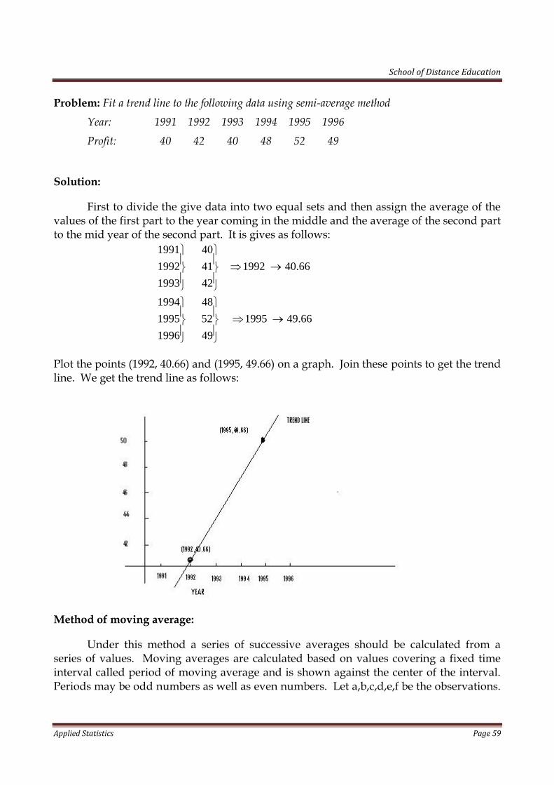
School of Distance Education
Applied Statistics Page 59
Problem: Fit a trend line to the following data using semi-average method
Year: 1991 1992 1993 1994 1995 1996
Profit: 40 42 40 48 52 49
Solution:
First to divide the give data into two equal sets and then assign the average of thevalues of the first part to the year coming in the middle and the average of the second partto the mid year of the second part. It is gives as follows:
1991 40
1992 41 1992 40.66
1993 42
1994 48
1995 52 1995 49.66
1996 49
Plot the points (1992, 40.66) and (1995, 49.66) on a graph. Join these points to get the trendline. We get the trend line as follows:
Method of moving average:
Under this method a series of successive averages should be calculated from aseries of values. Moving averages are calculated based on values covering a fixed timeinterval called period of moving average and is shown against the center of the interval.Periods may be odd numbers as well as even numbers. Let a,b,c,d,e,f be the observations.
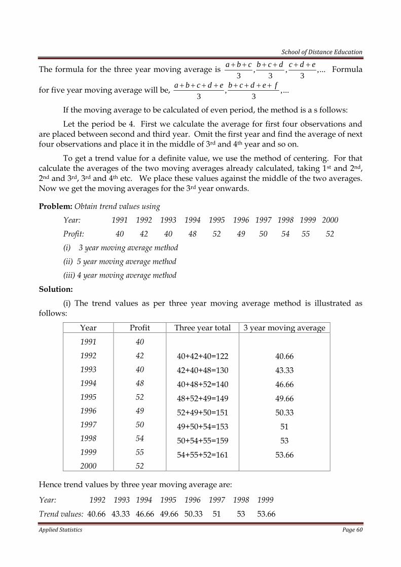
School of Distance Education
Applied Statistics Page 60
The formula for the three year moving average is , , ,...3 3 3
a b c b c d c d e Formula
for five year moving average will be, , ,...3 3
a b c d e b c d e f
If the moving average to be calculated of even period, the method is a s follows:
Let the period be 4. First we calculate the average for first four observations andare placed between second and third year. Omit the first year and find the average of nextfour observations and place it in the middle of 3rd and 4th year and so on.
To get a trend value for a definite value, we use the method of centering. For thatcalculate the averages of the two moving averages already calculated, taking 1st and 2nd,2nd and 3rd, 3rd and 4th etc. We place these values against the middle of the two averages.Now we get the moving averages for the 3rd year onwards.
Problem: Obtain trend values using
Year: 1991 1992 1993 1994 1995 1996 1997 1998 1999 2000
Profit: 40 42 40 48 52 49 50 54 55 52
(i) 3 year moving average method
(ii) 5 year moving average method
(iii) 4 year moving average method
Solution:
(i) The trend values as per three year moving average method is illustrated asfollows:
Year Profit Three year total 3 year moving average
1991
1992
1993
1994
1995
1996
1997
1998
1999
2000
40
42
40
48
52
49
50
54
55
52
40+42+40=122
42+40+48=130
40+48+52=140
48+52+49=149
52+49+50=151
49+50+54=153
50+54+55=159
54+55+52=161
40.66
43.33
46.66
49.66
50.33
51
53
53.66
Hence trend values by three year moving average are:
Year: 1992 1993 1994 1995 1996 1997 1998 1999
Trend values: 40.66 43.33 46.66 49.66 50.33 51 53 53.66

School of Distance Education
Applied Statistics Page 61
(ii) The trend values as per 5 year moving average method are illustrated as follows:Year Profit Five year total Three year
moving average
1991
1992
1993
1994
1995
1996
1997
1998
1999
2000
40
42
40
48
52
49
50
54
55
52
40+42+40+48+52=222
42+40+48+52+49=231
40+48+52+49+50=239
48+52+49+50+54=253
52+49+50+54+55=260
49+50+54+55+52=260
44.40
46.20
47.80
50.60
52
52
Hence trend values by five year moving average are:Year: 1993 1994 1995 1996 1997 1998Trend values: 44.40 46.20 47.80 50.60 52 52(iii) The trend values as per four year moving average method are illustrated as follows:
Year Profit Four year total Four yearaverage
Two term total Four yearmovingaverage
1991
1992
1993
1994
1995
1996
1997
1998
1999
2000
40
42
40
48
52
49
50
54
55
52
40+42+40+48=170
42+40+48+52=182
40+48+52+49=190
48+52+49+50=199
52+49+50+54=205
49+50+54+55=208
50+54+55+52=211
42.50
45.50
47.50
49.75
51.25
52
52.75
42.50+45.50=88
45.50+47.50=93
47.50+49.75=97.25
49.75+51.25=101
51.25+52=103.25
52+52.75=104.75
44
46.50
48.63
50.50
51.63
52.38

School of Distance Education
Applied Statistics Page 62
Hence trend values by four year moving average are:
Year: 1993 1994 1995 1996 1997 1998
Trend values: 44 46.50 48.63 50.50 51.63 52.38
Method of least squares:
Using the principle of least squares, we can find the linear as well as non lineartrend curves for a given time series data.
Linear trend: Using the method of fitting of a straight line, we can find a trend lineof the form y=ax+b for a given time series. The normal equations for finding a andb are
2
1 1 1
n n n
i i i ii i i
x y a x b x and
1 1
n n
i ii i
y a x n b
To reduce calculations, we apply a change of origin. Two cases may arise. Thenumber of years by the time series may be odd or even.
(i) If n is odd: We can take the origin at the middle year. Then x=0 willcorrespond to the middle year and x=1 for the next year and x=-1 for the
preceding year and so on. We shall then have,1
0n
ii
x
(ii) (ii) If n is even: (Let n=2m) Then there will be two middle years, the mth and(m+1)th year. We take the origin at the middle of these two years and take ahalf year as the unit. Then the mth year will correspond t x=-1 and (m+1)th
year to x=+1, and so on. We shall then have,1
0n
ii
x
.
Then the normal equation reduced to
2
1 1
n n
i i ii i
x y a x and
1
n
ii
y n b
Then, a and b is estimated as, 1
2
1
n
i ii
n
ii
x ya
x
and 1
n
ii
yb
n
.
In a similar way non-linear trend also can be estimated.
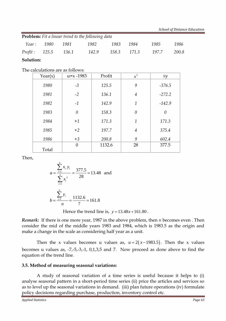
School of Distance Education
Applied Statistics Page 63
Problem: Fit a linear trend to the following data
Year : 1980 1981 1982 1983 1984 1985 1986
Profit : 125.5 136.1 142.9 158.3 171.3 197.7 200.8
Solution:
The calculations are as follows:Year(x) u=x -1983 Profit 2x xy
1980
1981
1982
1983
1984
1985
1986
-3
-2
-1
0
+1
+2
+3
125.5
136.1
142.9
158.3
171.3
197.7
200.8
9
4
1
0
1
4
9
-376.5
-272.2
-142.9
0
171.3
375.4
602.4
Total0 1132.6 28 377.5
Then,
1
2
1
377.513.48
28
n
i ii
n
ii
x ya
x
and
1 1132.6161.8
7
n
ii
yb
n
Hence the trend line is, 13.48 161.80y x .
Remark: If there is one more year, 1987 in the above problem, then n becomes even . Thenconsider the mid of the middle years 1983 and 1984, which is 1983.5 as the origin andmake a change in the scale as considering half year as a unit.
Then the x values becomes u values as, 2 1983.5u x . Then the x valuesbecomes u values as, -7,-5,-3,-1, 0,1,3,5 and 7. Now proceed as done above to find theequation of the trend line.
3.5. Method of measuring seasonal variations:
A study of seasonal variation of a time series is useful because it helps to (i)analyse seasonal pattern in a short-period time series (ii) price the articles and services soas to level up the seasonal variations in demand. (iii) plan future operations (iv) formulatepolicy decisions regarding purchase, production, inventory control etc.

School of Distance Education
Applied Statistics Page 64
Method of simple averages is an important method of studying seasonal variations.
(i) Method of simple averages:
The steps involved in this method are:
(i) Arrange the data by years, months or quarters as the case may be for asufficiently long period of time.
(ii) Obtain the monthly average from monthly data, or obtain quarterly averagefrom the quarterly data etc, for the whole period covered.
(iii) Obtain the overall average for a month or quarter from all the monthly orquarterly averages obtained.
(iv) Seasonal indices for different months are obtained on expressing eachmonthly or quarterly average as a percentage of the overall average.
If X is the overall average and kX is the monthly average for the kth month,
then, seasonal index for the kth month = 100kX
X .
Note: The sumo f seasonal indices must be 1,200 for monthly data and 400 for quarterlydata.
Problem: Use the method of monthly averages to determine quarterly indices for thefollowing data of production of a commodity based on years 1986, 1987, 1988.
Year(x)Production in lakhs of tonnes
1986 1987 1988
January
February
March
April
May
June
July
August
September
October
November
December
12
11
10
14
15
15
16
13
11
10
12
15
15
14
13
16
16
15
17
12
13
12
13
14
16
15
14
16
15
17
16
13
10
10
11
15

School of Distance Education
Applied Statistics Page 65
Solution:
Setting the data in quarterly form, we get as follows:
Year(x) Production in lakhs of tonnes
1986 1987 1988
First quarter
Second quarter
Third quarter
Fourth quarter
33
44
40
37
42
47
42
39
45
48
39
36
The calculations are as shown below:
Year(x)Production in lakhs of tonnes Quarterly
average1986 1987 1988
First quarter
Second quarter
Third quarter
Fourth quarter
33
44
40
37
42
47
42
39
45
48
39
36
40
46.33
40.33
37.33
Total average = 40 46.33 40.33 37.3340.9975
4
Hence the seasonal indices for the various quarters are:
For first quarter, indices is, 40100 97.57
40.9975 .
For second quarter, indices is, 46.33100 113.01
40.9975 .
For third quarter, indices is,. 40.33100 98.37
40.9975
For fourth quarter, indices is,. 37.33100 91.05
40.9975

School of Distance Education
Applied Statistics Page 66
EXERCISES
1. Define time series.
2. What are the various component of a tie series?
3. What are the additive and multiplicative models in time series?
4. Explain various components of time series.
5. What the methods of measuring trend in a time series?
6. Fit a trend line to the following data using semi-average method
Year: 1990 1991 1992 1993 1994 1995Profit: 34 34 34 34 32 39
7. Obtain trend values using
Year: 1990 1991 1992 1993 1994 1995 1996 1997 1998 1999Profit: 33 35 34 38 35 34 35 39 36 38(i) 3 year moving average method(ii) 5 year moving average method(iii) 4 year moving average method
8. Explain any method of measuring seasonal variation.
*********************

School of Distance Education
Applied Statistics Page 67
CHAPTER 4
STATISTICAL QUALITY CONTROL
4.1. Quality:
Quality means conformity with certain proscribed standards. These standards maybe in terms of size, weight, strength, colour, taste, etc. The quality standards are normallyset by the makers of the product. Government is also keen on quality standards. Onlyquality products are given ‘Agmark’ and ‘ISI’ labels.
Statistical Quality Control (SQC) refers to the statistical techniques employed forthe maintenance of uniform quality in a continuous flow of manufactured products.
Definition: “SQC is a simple statistical method for determining the extent to whichquality goals are being met without necessarily checking every item produced and forindicating whether or not the variation which occur are exceeding normal expectations.SQC enable us to decide whether to reject or accept a particular product”
Some of the advantages of Statistical Quality Control are
1. Quality of the product is effectively checked and deviation from the quality iseasily identified.
2. It protects the loss of buyer due to the rejection of the items purchased.
3. Quality consciousness among employees increased
4. SQC enable the producer to decide when to take corrective measures.
Apart from a company’s decision to produce every piece of quality item, some amountof variation among the item produced are observed. This may be mainly of two types ofcauses:
(1) Random and chance cause, which are some inevitable variations occurring and it isnatural and allowable and cannot be removed or prevented. (ii) Assignable andpreventable causes, which are neither natural nor inherent in manufacturing process andthey can be prevented if cause of such variation is identified.
The main purpose of SQC is to separate the preventable causes from the randomcauses.
4.2. Process and Product Control:
In a production process the quality is to be ensured. That is the proportion ofdefectives items is to be controlled. This is called process control. By product control wemean controlling the quality of the items produced by critical examination at strategicpoints.

School of Distance Education
Applied Statistics Page 68
4.3. Control chart:
Control chart is a statistical technique for process control. It is a graphical chartused to detect unusual variations occurring in the process of production that put theprocess out of control.
A control chart has three horizontal lines starting from the right hand side of thevertical line and parallel to the base line of the chart. The vertical line is meant forshowing the quality statistic of each sample and is known as quality scale. The base lineis used for making sample numbers and is termed as subgroup scale. The three horizontallines (i) central line (ii) upper control limit and (iii) lower control limit are known ascontrol lines.
Central line (CL): It passes through the middle of the chart parallel to the base line andrepresents the prescribed standard of quality of the product in the process. If themanufacturing process in in the perfect state of control and the product producedconforms perfectly to the prescribed standards, the sample points will coincide with thisline.
Lower Control Line (LCL): This is dotted line parallel to and below the central line. Thisline represents the maximum lowest limit of variation that can tolerate.
Upper Control Line (UCL): This is dotted line parallel to and above the central line. Thisline represents the maximum highest limit of variation that can tolerate.
If the sample points are lying in between these dotted lines in control chart, it isassumed that the variation in the process is wholly due to chance cause and the process isunder control. Otherwise some assignable causes are involved in the process and theprocess is considered as out of control and the remedial measures are to be executed.
Control chart for variables:
To control the quality of a characteristic which are measurable, like diameter of ascrew, specific resistance of a wire etc, we use two types of control charts. They are chartsfor x (mean) and charts for R (range)
p-chart:
This type of chart are used to deal with the characteristics which are not possible tomeasure, but can observe as absent or present from the product classifying as defective ornon defective.
c-chart:
This type of chart is applicable when the quality of product is a discrete variable
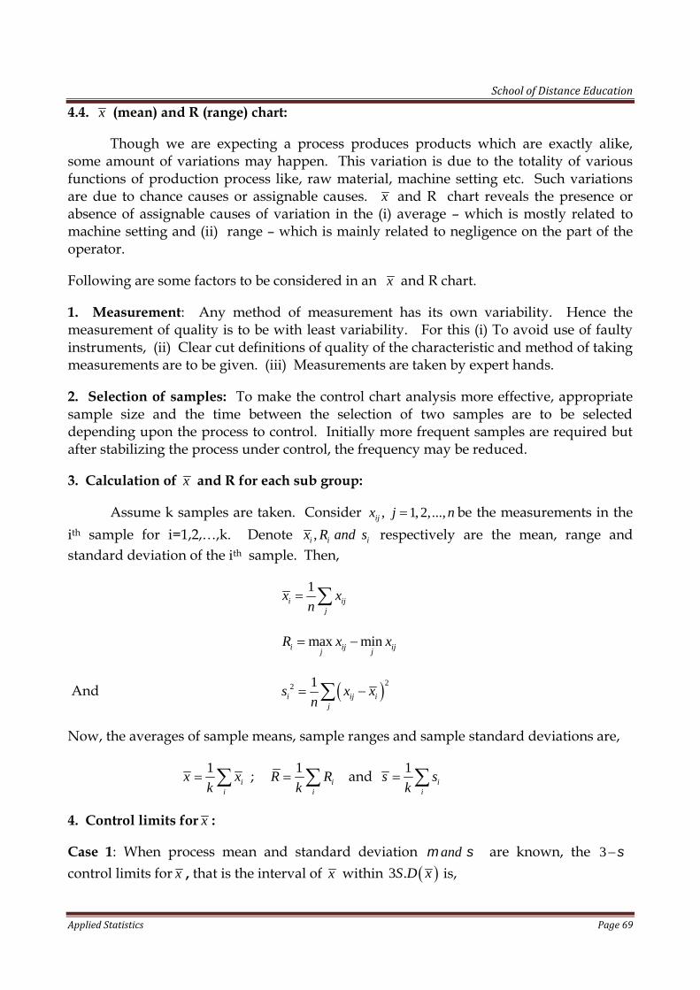
School of Distance Education
Applied Statistics Page 69
4.4. x (mean) and R (range) chart:
Though we are expecting a process produces products which are exactly alike,some amount of variations may happen. This variation is due to the totality of variousfunctions of production process like, raw material, machine setting etc. Such variationsare due to chance causes or assignable causes. x and R chart reveals the presence orabsence of assignable causes of variation in the (i) average – which is mostly related tomachine setting and (ii) range – which is mainly related to negligence on the part of theoperator.
Following are some factors to be considered in an x and R chart.
1. Measurement: Any method of measurement has its own variability. Hence themeasurement of quality is to be with least variability. For this (i) To avoid use of faultyinstruments, (ii) Clear cut definitions of quality of the characteristic and method of takingmeasurements are to be given. (iii) Measurements are taken by expert hands.
2. Selection of samples: To make the control chart analysis more effective, appropriatesample size and the time between the selection of two samples are to be selecteddepending upon the process to control. Initially more frequent samples are required butafter stabilizing the process under control, the frequency may be reduced.
3. Calculation of x and R for each sub group:
Assume k samples are taken. Consider , 1, 2,...,ijx j n be the measurements in theith sample for i=1,2,…,k. Denote ,i i ix R and s respectively are the mean, range andstandard deviation of the ith sample. Then,
1i ij
j
x xn
max mini ij ijjj
R x x
And 22 1i ij i
j
s x xn
Now, the averages of sample means, sample ranges and sample standard deviations are,
1i
i
x xk ; 1
ii
R Rk and 1
ii
s sk
4. Control limits for x :
Case 1: When process mean and standard deviation and are known, the 3
control limits for x , that is the interval of x within 3 .S D x is,

School of Distance Education
Applied Statistics Page 70
3 . . , 3 . .E x S D x E x S D x
That is, 3 , 3n n
Then, 3xLCLn
; 3xUCL
n
Case 2: When and are unknown.
Then and are estimated by x and2
R
d, where 2d is a constant depending upon
the sample size. Then the 3 control limits for x is,
2 2
1 13 , 3
R Rx x
d dn n
Then,2
13x
RLCL x
d n ;
2
13x
RUCL x
d n
A table of the values of2
3
d nis available for different values of n from 2 to 25.
can be estimated using s also, by the expression,2
s
c , where 2
2!
2 2.
3!
2
n
cnn
A table of the values of2
3
c nis available for different values of n from 2 to 25.
5. Control limits for R chart:
3 limit for R chart is
3 , 3 1 3 , 1 3R cR R cR c R c R , where c is a constant depending upon n.
The values of 1 3 1 3c and c are listed in table for various values of n.
1 3RLCL c R and
1 3RUCL c R

School of Distance Education
Applied Statistics Page 71
Construction of x chart:
x Chart is constructed with sample number is taken along axis and thecorresponding sample mean ix is taken along is taken along Y-axis. The points areplotted but not joining. The central line is drawn as bold parallel to X-axis along the valuemean of the sample means x .
Upper Control Limit line and Lower Control Limit line are drawn as dotted linesparallel to X axis through the calculated Y values, xUCL and xLCL respectively.
The points fall beyond the control lines, if any, indicates assignable causes makes theprocess out of control. Now remove all the sample results which are beyond the controllimits or revise the control limits for the remaining samples. Revision of control limit isrepeated so as the entire sample means are within the new control limits. The new limitsare then extended for checking the quality of future products.
Construction of R- chart:
Since small samples of size 2-15, range provides a good estimate of , range iscommonly used in SQC to study the pattern of variation in quality.
To draw R-Chart, we proceed as done in the case of x Chart. Take sample numberalong X- axis and the corresponding sample range iR is taken along Y-axis. Central lineparallel to X-axis is drawn as bold line through R and the control lines are drawn throughthe calculated values of RLCL and RUCL as dotted lines parallel to X-axis. Since range isnon-negative, RLCL must be non-negative. If it is calculated as negative in any case, it isconsidered as zero.
Note:
(i) x Chart is used to show the quality averages of the samples drawn from a givenprocess, whereas R chart is used to show quality dispersions of the samples.
(ii) Usually R chart is drawn first. If R chart indicates that the dispersion of the quality bythe process is out of control it is better not to construct x Chart until the quality dispersionis brought under control.
(iii) For a normal population probability of any point falling outside the 3 control lineis only 0.0027. If a point falls outside the limits it will be desirable to take another biggersample. If the mean o the combined samples still lie out of the control limits there shouldbe search for assignable causes.
Problem: Construct a control chart for mean and the range for the following data on thebasis of fuses, samples of 5 being taken every hour (each set of 5 has been arranged inascending order of magnitude).
42 42 19 36 42 51 60 18 15 69 64 61
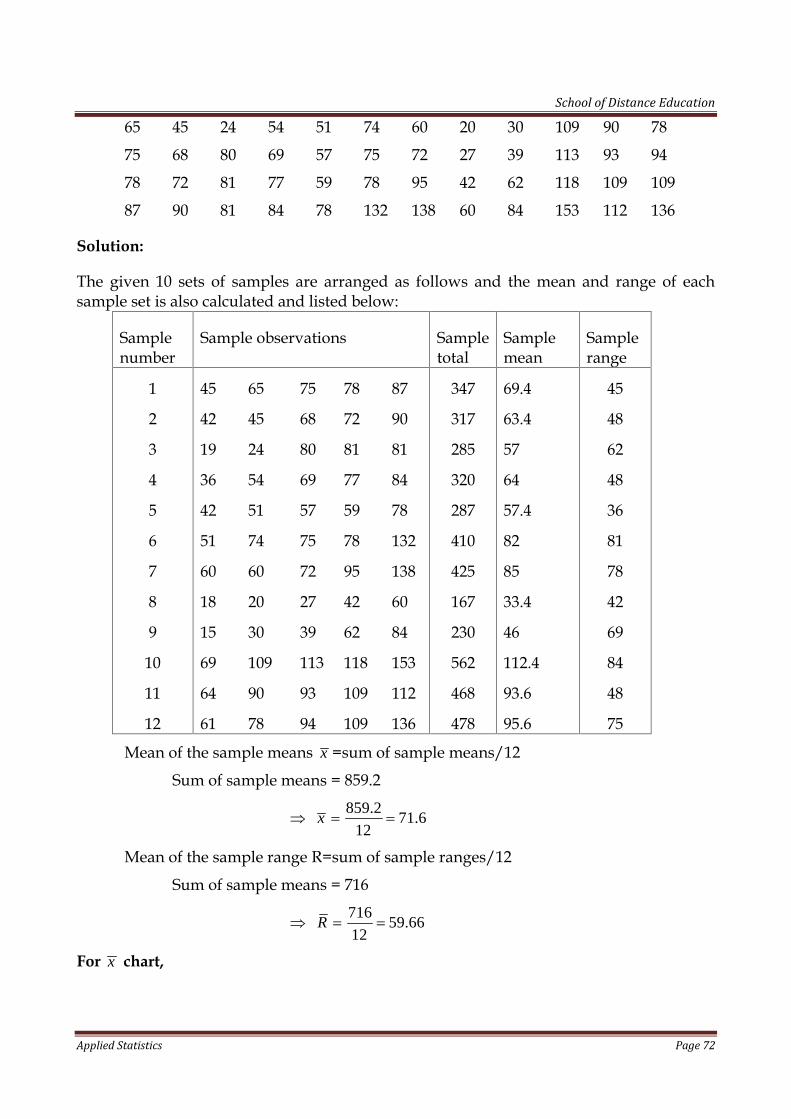
School of Distance Education
Applied Statistics Page 72
65 45 24 54 51 74 60 20 30 109 90 78
75 68 80 69 57 75 72 27 39 113 93 94
78 72 81 77 59 78 95 42 62 118 109 109
87 90 81 84 78 132 138 60 84 153 112 136
Solution:
The given 10 sets of samples are arranged as follows and the mean and range of eachsample set is also calculated and listed below:
Samplenumber
Sample observations Sampletotal
Samplemean
Samplerange
1
2
3
4
5
6
7
8
9
10
11
12
45 65 75 78 87
42 45 68 72 90
19 24 80 81 81
36 54 69 77 84
42 51 57 59 78
51 74 75 78 132
60 60 72 95 138
18 20 27 42 60
15 30 39 62 84
69 109 113 118 153
64 90 93 109 112
61 78 94 109 136
347
317
285
320
287
410
425
167
230
562
468
478
69.4
63.4
57
64
57.4
82
85
33.4
46
112.4
93.6
95.6
45
48
62
48
36
81
78
42
69
84
48
75
Mean of the sample means x =sum of sample means/12
Sum of sample means = 859.2
859.271.6
12x
Mean of the sample range R=sum of sample ranges/12
Sum of sample means = 716
71659.66
12R
For x chart,

School of Distance Education
Applied Statistics Page 73
2
13x
RLCL x
d n ;
2
13x
RUCL x
d n The value of
2
3
d nfor n=5 is obtained
from table as, 0.58
Hence,
71.60 59.66 0.58 37xLCL ; 71.60 59.66 0.58 106.2xUCL .
For R chart,
The values of 1 3 1 3c and c for n=5 are, 0 and 2.11
Hence, 1 3RLCL c R =0 and
1 3 2.11 59.66 126.181RUCL c R
The charts are drawn as follows:

School of Distance Education
Applied Statistics Page 74
Since one point is beyond the control lines, the x bar chart says that there is a lackof control in process average and it suggests the presence of some assignable causes whichis to be detected and corrected.
Since all the points in R chart are within the control lines, the process variability isunder control.
4.5. p-Chart:
p-chart is the control chart for defectives. Whenever the quality characteristic ismeasured as yes or no, that is absent or present or like defective or non-defective p-chartis used. Consider n items are observed and d items of them are defectives, then d is abinomial variable with parameters n and P. P –the fraction of defective for a sample isestimated by d/n.
To draw p-chart, obtain the values of P for each sample. Then obtain the averagefraction defective from all the samples combined as,
.
.
No of defectives in all samples combinedP
Total no of items in samples comibined
Now the upper control limit and lower control limit of p-chart at 3 sigma level is obtainedas
3 ; 3P PUCL P LCL P
Where
(1 ) /P P n , which is estimated by (1 ) /P P n .
Hence,
3 (1 ) / ; 3 (1 ) /P PUCL P P P n LCL P P P n
Since P is ever negative, if PLCL is found as negative, consider it as zero.
Draw the central line, which is the horizontal line through P .
Plot the fraction of defective for each sample and find whether all the points are within thecontrol lines or not.
A point appears above the PUCL indicates the lack of control and process changedfor the worse. Such a point is called high spot.
A point appears below the PLCL indicates the process changed for better. Such apoint is called low spot which indicates improvement in quality.

School of Distance Education
Applied Statistics Page 75
4.6. d-Chart:
d-chart is similar to p-chart, but in this chart instead of plotting the fraction ofdefective for each sample, the number of defective for each of the sample is plottedagainst the corresponding sample number.
The lines of control are:
Central line is passing through the value of nP, where P is the probability ofdefective. If P is unknown it is estimated from the average number of defectives persample of constant size as,
.
.
No of defectives in all samples combinedP
Total no of items in samples comibined
The UCL corresponds to 3-sigma level is,
3 (1 )nP nP P ; n is the sample size (constant)
When P is not given, UCL is 3 (1 )nP nP P
LCL is 3 (1 )nP nP P or 3 (1 )nP nP P
LCL value is kept as zero, if it is calculated as negative.
Problem: The following data refer to visual defects found during inspection of the first 10samples of size 100 each. Use them to obtain upper and lower control limits forpercentage effective in samples of 100.
Sample No. 1 2 3 4 5 6 7 8 9 10
4 8 11 3 11 7 7 16 12 6
Solution:
The total number of defectives in the given set of 10 samples of 100 each is 85.
Hence, . 850.085
. 1000
No of defectives in all samples combinedP
Total no of items in samples comibined
Central line is passing through nP = 100 0.085 8.5
3 (1 ) 100 0.085 3 100 0.085(1 0.085)UCL nP nP P =18.87
3 (1 ) 100 0.085 3 100 0.085(1 0.085)LCL nP nP P =0.134

School of Distance Education
Applied Statistics Page 76
The chart is drawn as follows:
Since all the points are within the control lines, the process is under control.
Note: If the number of items inspected n in each sample varies, for p- chart separatecontrol limits have to be computed for each sample while the central line has to becomputed for each sample. These types of limits are known as variable control limits. Insuch a situation p-chart is relatively simple and preferred.
4.7. C-Chart ( Control chart for number of defects per unit):
A defective item may contain one or more defects. In p-chart or in d-chart thenumbers of defectives are counted, but not concentrating on the number of defects perunit. C-chart is concentrating on the number of defects per unit in a sample of items withconstant size.
Control limits of C-chart:
While inspecting a large sample, if the numbers of defectives are less, the probability p ofoccurrence of a defect in any unit is very small. Hence Poisson approximation to thenumber of defect is appropriate and the control limit calculation is based on Poissondistribution.
When the number of defect is Poisson distributed variable, the average number ofdefect is the parameter
If is known, the 3-sigma level, UCL= 3 and
LCL= 3
Central line is passing through
If is unknown, is estimated by

School of Distance Education
Applied Statistics Page 77
.ˆ .total no of defects
average no of defectstotal units observed
Then, central line is through ̂ ,
UCL= ˆ ˆ3 and
LCL= ˆ ˆ3 (which is taken as zero, if calculated as negative)
EXERCISES
1. What is Statistical Quality Control (SQC)?
2. Distinguish between process control and product control.
3. What is a control chart?
4. Write a short note on the lines of control.
5. What are the things to be considered while drawing x bar chart?
6. Explain R chart.
7. Which control charts are used in the case of attributes? Explain.
8. Draw the mean and range charts and comment for the following data
Sample No. 1 2 3 4 5 6 7 8 9 10
Mean 43 49 37 44 45 37 51 46 43 47
Range 5 6 5 7 7 4 8 6 4 6
9. Discuss the construction of p chart when all samples are of same size.
10.During an examination of equal length of cloth, the following are the number ofdefects observed:
2,3,4,0,5,6,7,4,3,2
Draw control chart for the number of defects and comment whether the process isunder control or not.
************************

School of Distance Education
Applied Statistics Page 78
CHAPTER 5
ANALYSIS OF VARIANCE
5.1. Analysis of Variance (ANOVA)
To test the difference between the means of two normal populations are testedusing t-distribution. But to test the means of three or more population together based onsamples taken from them is not possible with t-test. Analysis of variance, ANOVAprovides a statistical test of whether or not the means of several groups are all equal, andtherefore generalizes t-test to more than two groups. Doing multiple two-sample t-testswould result in an increased chance of committing a type I error. For this reason,ANOVAs are useful in comparing two, three, or more means.
Analysis of variance was introduced by Prof.R.A.Fisher in 1920’s.
Assumptions in ANOVA
The populations from which the samples were obtained must be normally orapproximately normally distributed.
The samples must be independent.
The variances of the populations must be equal.
5.2. One way ANOVA
Let the data are classified according to only one characteristic. Considerindependent sample of 1 2, ,... kn n n observations from different populations with populationmeans 1 2, ,... k . Then one way ANOVA is to test the arithmetic means of thepopulation from which the k samples are randomly drawn are equal to one another or it isto test the hypothesis 0 1 2: ... kH .
Procedure for One way ANOVA
Let us consider, we have k independent samples. Assume samples containingrespectively 1 2, ,... kn n n items. Let ijx denotes the ith observation in the jth class. The totalnumber of items in the sample is 1 2 ... kn n n n . Total variation among theobservations are classified into two (i) variation between the samples (or classes ortreatments) and (ii) variation within the sample. The first type of variation is due toassignable causes, while the second type of variation is due to chance. Main aim ofanalysis of variance is to examine whether the means of all populations from the samplesare taken are same in view of the variability within the samples (classes).

School of Distance Education
Applied Statistics Page 79
The steps for ANOVA for testing 0 1 2: ... kH are listed as follows:
Step1: Obtain the sample means of each of the k samples. Let it be 1 2, ,..., kx x x .
Step 2: The grand average of the entire n sample items X is found as 1 2 ... kx x xX
k
,
where k is the total number of samples.
Step 3: Take the difference between the means of the various samples and the grandaverage.
Step 4: Find the sum of squares of these differences. This number is the sum of squaresbetween the samples (SSB).
Step 5: Mean sum of squares between the samples is1
SSBMSB
k
.
Step 6: Take the deviations of the various items in a sample from the mean of therespective sample and add the squares of such deviations. This number is the sum ofsquares within the samples (SSW).
Step 7: Mean sum of squares within the samples is SSWMSW
n k
.
Step 8: Calculate F-ratio, where the ratio MSBF
MSW .
Step 9: Compare the calculated F with the table value of F-distribution with degrees offreedom 1,k n k .
Step 10: If calculated value of F is less than the table value, ACCEPT the hypothesis thatthe population means are equal.
ANOVA table for one way classified data:
Source of variation Sum ofsquares
Degrees offreedom
Mean sum ofsquares
F- ratio
Between Sample
(class or treatment) SSB k-1 MSB=SSB/k-1
MSBF
MSWWithin samples (or
Error)SSW n-k MSW=SSW/n-k
Total SST n-1

School of Distance Education
Applied Statistics Page 80
Illustration:
Consider a sample of three bulbs is taken from four companies producing lightbulbs. Their lifetimes in hours are tested and the results in hundreds of hours are asfollows.
Companies
A B C D
18
17
15
20
16
15
18
16
16
15
18
15
Test whether the mean lifetime of the bulbs from the four companies are equal.
Solution:
Let the mean life of the bulbs produced by the four companies are 1 2 3 4, , and
To test 0 1 2 3 4:H .
The means of the samples, 1
18 17 1516.67
3x
2
20 16 1517
3x
; 3
18 16 1616.67
3x
and 4
15 18 1516
3x
Hence the grand mean, 16.67 17 16.67 1616.585
4X
Sum of squares between the samples SSB = 2 2 2 216.67 16.585 17 16.585 16.67 16.585 16 16.585
0.007225 0.172225 0.007225 0.342225
= 0.5289.
Then,
MSB 0.52890.1763
3 .
Sum of squares between the samples SSW is calculated as follows:
For the samples from company A: 1 16.67x ;
The sum of squares of deviation = 2 2 218 16.67 17 16.67 15 16.67
=1.7689 0.1089 2.7889 4.6667
For the samples from company B: 2 17x ;
The sum of squares of deviation = 2 2 220 17 16 17 15 17

School of Distance Education
Applied Statistics Page 81
= 9 1 4 14 .
For the samples from company C: 3 16.67x ;
The sum of squares of deviation = 2 2 218 16.67 16 16.67 16 16.67
= 1.7689 0.4489 0.4489 2.6667 .
For the samples from company D: 4 16x ;
The sum of squares of deviation = 2 2 215 16 18 16 15 16
= 1 4 1 6 .
Hence,
SSW = 4.6667 14 2.6667 6 27.334
4.6667 14 2.6667 6
8MSW
=3.4167
0.17630.0516
3.4167
MSBF
MSW
The table is,
Source of variation Sum ofsquares
Degreesof
freedom
Mean sum ofsquares
F- ratio
Between Sample(class or treatment)
SSB=0.5289. 4-1 MSB 0.1763
0.17630.0516
3.4167F Within samples (or
Error)SSW27.334
12-4 MSW=3.4167
Total SST=27.8629 11
From table of F distribution, table value for (3,8) d.f. at 5% significance level is 4.07
Here, calculated F value is less than the table F value. Hence ACCEPT thehypothesis that the mean lifetimes of the bulbs from the four companies are equal.
5.3. Two way ANOVA:
In one way ANOVA, we considered a variable influenced by various levels(treatments) of a factor. Our test was, whether all treatments are alike with respect to theirmean effect or not. But in two way ANOVA, we consider a variable which is influencedby various levels of two factors. It is to test whether these factors have any impact on thevariable.

School of Distance Education
Applied Statistics Page 82
Consider the case of the study of the effect of m variety of training methods and nvariety of foods on the intelligent quotient of mXn students.
Let ijx be the intelligent quotient of a student with ith training and jth food.
Suppose mXn students are divided in to m groups, where ith group receives the ith
training program for i-1,2,…,m and let these students are also divided into n groups,where jth group receives the jth food for j=1,2,…,n. Let us consider the data on IQ is listedas follows;
Let us given the data on IQ as follows:
11 12 1
21 22 2
1 2
1 2 ...
...1
...2
: : ... ::
...
m
m
n n nm
Training group
m
x x x
x x xFood group
x x xn
Here the hypothesis is 0 1 2
1 2
: ...
: ...m
n
H
Where i is the mean IQ due to ith training and j is the mean IQ due to jth food.
The steps for two way ANOVA are listed as follows:
Step1: Obtain the means of each of the m columns. Let it be 1* 2* *., ,..., mx x x .
Obtain the means of each of the n rows. Let it be *1 *2 * ., ,..., nx x x .
Step 2: The grand average of the entire n sample items X is found as 1ij
i j
X xnm ,
Step 3: Take the difference between the means of the various samples and the grandaverage.
Step 4: Sum of squares between the treatments of food (SSR)= 2*ii
m x X
Step 5: Mean sum of squares due to the treatments of various food is1
SSRMSR
n
.
Step 6: Sum of squares between the treatments of training (SSC)= 2* ji
n x X
Step 7: Mean sum of squares due to the treatments of various food is1
SSCMSC
m
.

School of Distance Education
Applied Statistics Page 83
Step 8: Total sum of squares SST= 2iji j
x X
Step 9: Error sum of square SSE= 2* *ij i ji j
x x x X
Step 10: Error Mean sum of square MSE= 2* *
1
1 1 ij i ji j
x x x Xm n
Calculate F-ratio, where the ratio R
MSRF
MSE follow 1,( 1)( 1)n m nF .
Step 11: Compare the calculated F with the table value of F-distribution withdegrees of freedom 1, ( 1)( 1)n m n .
Step 12: If calculated value of F is less than the table value, ACCEPT thehypothesis that the effects of food are equal.
Calculate F-ratio, where the ratio C
MSCF
MSE follow 1,( 1)( 1)m m nF .
Step 13: Compare the calculated F with the table value of F-distribution withdegrees of freedom 1, ( 1)( 1)m m n .
Step 14: If calculated value of F is less than the table value, ACCEPT thehypothesis that the effects of trainings are equal.
EXERCISES11.Define ANOVA.
12.What are the assumptions in ANOVA
13.Differentiate between one way and two way ANOVA.
14.What is a control chart?
15. Explain the procedures of one way ANOVA.
16.Explain the situation where we are using two way ANOVA.
17.Explain the procedures of two way ANOVA.
18.The following table shows the lives in hours of four batches of electricbulbs.
Batch 1: 1600 1610 1680 1700 1720 1800
Batch 2: 1710 1590 1610 1700 1670 1600
Batch 3: 1650 1580 1680 1670 1630 1560
Batch 4: 1750 1680 1570 1680 1620 1660
Perform an ANOVA on these values and show that a significance test doesnot reject their homogeneity.
********************