
School of Accounting - UNSW Business School...Davis, the University of Otago, and the Auckland...
56
School of Accounting Seminar – Session 2, 2011 The Relevance to Investors of Greenhouse Gas Emission Disclosures Professor David Lont University of Otago Date: Friday 21 st Time: 3:00 to 4:30 pm October Venue: ASB130
Transcript of School of Accounting - UNSW Business School...Davis, the University of Otago, and the Auckland...
School of Accounting
Seminar – Session 2, 2011
The Relevance to Investors of Greenhouse Gas Emission Disclosures
Professor David Lont University of Otago
Date: Friday 21st
Time: 3:00 to 4:30 pm October
Venue: ASB130
The Relevance to Investors of
Greenhouse Gas Emission Disclosures
By Paul A. Griffin1, David H. Lont2 & Yuan Sun3
1 University of California, Davis 2 University of Otago 3 University of California, Berkeley
October 3, 2011.
We thank Shannon Anderson, Mike Bradbury, Steve Cahan, Scott Chaput, Peter Clarkson, Nina Dorata, Roger
Edelen, David Hay, Gordon Richardson, and a reviewer for the American Accounting National Meetings, Denver,
for their comments. This paper also incorporates the comments from presentations at the University of California,
Davis, the University of Otago, and the Auckland Business School 2011 Quantitative Accounting Research
Symposium. Comments welcome. Version of October 3, 2011.
Corresponding author: Paul A. Griffin, Graduate School of Management, University of California, Davis, 95616-
8609. 1-530-752-7372 (tel.), 1-425-799-4143 (fax), [email protected] (e-mail). All errors and omissions are
ours.
ii
The Relevance to Investors of
Greenhouse Gas Emission Disclosures
Abstract
This study documents that investors care about companies’ greenhouse gas (GHG) emission disclosures. Three kinds of evidence support this finding. First, using companies that disclose GHG emissions voluntarily through the Carbon Disclosure Project (CDP), we show that investors act as if they use GHG emission information to assess company value. Second, our evidence finds that investors view estimates of non-disclosed GHG emission amounts as value relevant, suggesting that stock prices reflect GHG information from channels other than CDP disclosure. Third, we conduct an event study and observe a significant stock market response when companies disclose climate change information in an 8-K filing. Our results strengthen for GHG-intensive industries such as utilities, energy, and materials companies, whose valuation effects are more negative. Economically, our results suggest that for every ton of GHG emitted by the median company in our sample at an assumed cost of $20 per ton, the stock market recognizes about 35-50 percent of that amount as an off-balance sheet liability.
JEL Classification: G14, M41, M45, K22, Q20.
Keywords: Greenhouse gas emissions, investor relevance, climate change reporting, S&P 500 companies, TSE 200 companies, U.S. and Canadian disclosure regulations, EPA Rule 40 CFR Part 98, stock market impact, event study.

1
The Relevance to Investors of
Greenhouse Gas Emission Disclosures
1 Introduction
Companies today face a daunting challenge of what and how much to disclose publicly about
the risks and costs of climate change. On the one hand, investors and public interest groups
worldwide call for more disclosure, greater uniformity, and more transparency. Companies and
insurers, on the other hand, worry about the costs of disclosure, particularly from competitive
disadvantage and liability exposure, and press for a more balanced consideration of the costs and
benefits. This study focuses on an essential element of this debate, namely, whether stock investors
view climate change disclosures by companies as relevant for valuation purposes, where investor
relevance means that the disclosures relate to investors’ reassessment of stock price conditional on
the total mix of available information. As explained below, such findings can be critically
important for companies’ disclosure decisions, regulators’ views on mandating climate change
reporting and disclosure, investors’ and analysts’ understandings of the role of climate change
information in pricing stocks, and courts’ determinations in adjudicating securities laws on climate
change and environmental issues.
We focus our investigation on greenhouse gas (GHG) emission disclosures, which many
companies now reveal voluntarily, in response to the needs of investors and analysts. We further

2
restrict our analysis to S&P 500 and Toronto Stock Exchange (TSE) 200 companies to assess the
relevance of carbon emissions for large companies in two environments. As evidence of investor
relevance, we find that (1) investors care about GHG emissions in assessing company value and (2)
GHG emission information in a company press release or 8-K filing elicits a significant price and
trading reaction around the day of the report as investors update their expectations. We further find
that investors’ valuations and responses differ on the basis of GHG emission intensity, where
higher intensity associates negatively with stock price and news response. Our valuation results are
also economically interpretable. We calculate that for every ton of GHG emitted by the median
company in our sample at an assumed cost of $20 per ton, the stock market recognizes about 35-50
percent of that amount as an off-balance sheet liability.
In addition, we estimate GHG emissions for S&P 500 and TSE 200 companies that do not
report GHG emissions and control for possible sample selection bias. We find that estimated
GHGs also relate to market prices in much the same manner as disclosed GHGs. This suggests that
stock prices reflect GHG information irrespective of whether the company makes a formal
disclosure. This is central to the debate because it implies that non-disclosers’ stock prices are not
devoid of GHG information, contrary to the beliefs of some advocates who contend capital markets
need full disclosure to solve an information deficiency.1 Advocates’ and regulators’ proposals that
focus on full disclosure rather than incremental information relative to the total mix might also be 1 For instance, Young et al. (2009), in a project sponsored by Ceres and the Environmental Defense Fund, state as follows regarding the conclusions of their 2008 disclosure survey. “Absent SEC action, investors are left in the dark about companies’ plans for evaluating and managing material risks in a changing climate.” (p. iv).

3
economically wasteful in the context of market efficiency.
These results add to the literature in several unique ways. First, we extend earlier results on
the market pricing of environmental obligations by focusing on the market’s off-balance sheet
recognition of GHG emission obligations, now even more relevant to company disclosure policy
because of the legal standing of emissions and climate change in Massachusetts v. EPA (127 Sup.
Ct. 1438,1440). Second, we extend a nascent empirical literature on the value relevance of GHG
emissions to investors by documenting predictable valuation and disclosure effects for GHG
discloser and non-discloser companies in two economic environments (the United States and
Canada). We use a research design that exploits variation in emissions cross-sectionally and
temporally, and we use an event study approach to measure short-term announcement effects. Our
dual approach produces reliable evidence across the two perspectives in support of our hypotheses.
Third, our results should also be important for evolving regulatory guidance on what companies
should disclose to investors about GHG emissions and climate change in that we document investor
relevance for such disclosures.2
Our paper continues as follows. Section 2 discusses key features of the institutional
2 Although investor relevance (an economic concept) does not equate to materiality (a legal concept), courts have often viewed a statistically significant stock price adjustment reliably attributable to a disclosure as dispositive in testing for materiality, and in some instances courts have wed the two concepts on pragmatic grounds. As such, our results should also be of interest to companies and regulators about whether GHG information might be ex ante material. Barth et al. (2001) also discuss why investor or “value relevance” might have implications for accounting rule makers, such as the Financial Accounting Standards Board. The FASB has yet to issue standards on uniform accounting and reporting for climate change, in particular, standards for emission obligations under a cap-and-trade system (FASB 2007, 2008, 2010).

4
environment and relevant prior research. Section 3 summarizes the data, sample, and research
design to test our expectations. Section 4 presents the results, section 5 describes additional
analysis and robustness tests, and section 6 concludes.
2 Institutional features and prior research
2.1 Institutional features
Many U.S. and Canadian companies disclose GHG emissions voluntarily through the Carbon
Disclosure Project (CDP), a U.K. organization representing mostly institutional investors. CDP
works with large companies worldwide to measure and manage their emissions and climate change
strategies and collects and publishes emissions data as part of its annual surveys. Companies may
decline to participate or simply not reply, but CDP tracks such indications so that each survey
covers a well-defined sample, such as the S&P 500 or TSE 200. The proportion of companies in
our sample reporting GHG emissions to the CDP has grown over the years studied, for example,
from 29 percent in 2006 to 53 percent in 2009 for the S&P 500, with a similar trend but lower
percentages for the TSE 200 (table 1).
Heightened investor interest and pressure from public interest advocates such as Ceres and
Friends of the Earth3 doubtlessly account for some of this growth, but company incentives may also
be a factor if investors view nonparticipation negatively. Required disclosure is also a reality for 3 For example, Ceres’ Web site (www.ceres.org) states as its mission “integrating sustainability into capital markets for the health of the planet and its people.” Friends of the Earth states that it “seeks to change the perception of the public, media and policy makers – and effect policy change – with hard-hitting, well-reasoned policy analysis and advocacy campaigns that describe what needs to be done, rather than what is seen as politically feasible or politically correct.” (www.foe.org).

5
some U.S. companies, but this is not yet at the federal level, with the possible exception of EPA
Rule 40 CFR Part 98 (EPA 2009), which will apply to large U.S. emitters following
implementation in 2011.4
Rather than set forth specific rules for measuring and disclosing climate change risk, U.S. and
Canadian securities regulators have, thus far, issued guidance releases only on their existing
disclosure frameworks. In the United States, Release 33-9106 (SEC 2010) outlines the SEC’s
views on what constitutes compliance with existing disclosure laws such as Regulation S-K, Item
101, on compliance with environmental laws, and Item 103 on environmental litigation. Regulation
S-K further requires disclosure of material risks and trends as either a separate section or as part of
management’s discussion and analysis. Such risks and trends arguably include climate change
factors such as GHG emissions.
Parallel regulations also obligate Canadian companies to disclose material information to
investors, such as CSA National Instrument 51-102 (CSA 2004), which is similar to Item 103 of
Regulation S-K, and CSA Annual Information Form, which is similar to a combined 10-K and
DEF-14A filing. Also, CSA Staff Notice 51-333 (2010) provides additional guidance for Canadian
companies on how National Instrument 51-102 applies to environmental risk, trends and
uncertainties, liabilities, and the financial and operational effects of environmental laws.
4 Also, at the state level, some attorneys general have used litigation to force additional disclosure of climate change risk, such as New York State’s application of the fraud provision (section 352) of the Martin Act of 1921 to Xcel Energy and Dynegy (Attorney General of the State of New York 2008a, 2008b). In addition, California recently approved a cap-and-trade plan with mandatory GHG reporting beginning in 2011 for entities emitting more than 25,000 tons of GHG annually (California Air Resources Board 2010).

6
Interestingly, regarding materiality, Staff Notice 51-333 states that many investors and shareholders
“think that, in some cases, material information regarding environmental matters is found in
voluntary reports and not in regulatory filings,” but that such information is “not necessarily
complete, reliable or comparable among issuers” and is “not necessarily provided in a timely
manner.” (p. 4). This document also refers specifically to “voluntary reports” as those relating to
the CDP (p. 24). In other words, in some cases, some regulators see voluntary disclosures as
potentially material but not necessarily sufficient from a rule-making perspective.
While our evidence in this paper might buttress regulators’ and disclosure advocates’ views on
the usefulness of climate change information for assessing stock return, our results also have
implications for companies and their insurers, in that any system of required disclosure ups the ante
on competitive disadvantage, litigation risk (Barth et al. 1997, Erion 2009), and liability exposure
for insurance purposes (Allen et al. 2009, Weigand 2010). Investors, typically, do not sue
companies for failure to follow voluntary guidelines but, rather, for failure to adhere to mandated
rules and regulations. On the other hand, companies sued for failure to disclose material climate
change items might note the evidence in this study about non-discloser companies, which suggests
that climate change information may be telegraphed to investors through channels other than CDP
disclosure.
2.2 Prior research
The most relevant prior literature relates to work on the valuation effects of environmental

7
disclosures.5 The categories studied include examination of the relation between environmental
liabilities and stock price (Barth and McNichols 1994, Lim and McConomy 1999, Campbell et al.
2003), how environmental and social responsibility disclosures relate to the cost of equity or debt
(Blacconiere and Patton 1994, Campbell et al. 1998, Konar and Cohen 2001, Plumlee et al. 2008,
Stanny and Ely 2008, Bauer and Hann 2010, Clarkson et al. 2010, Dhaliwal et al. 2010), whether
SO2 emissions have valuation relevance for investors (Hughes 2000, Johnston et al. 2008), and
whether investors find carbon emissions as value relevant (Chapple et al. 2011, Matsumura et al.
2011).
These studies also provide a basis for our primary research expectation of a negative relation
between GHG emissions and stock price. We reason that higher emissions will drain more cash
flow from the company in the form of higher future compliance, abatement, regulatory, and tax
costs not already reflected in the market’s assessments of reported earnings and shareholders’
equity (and other control variables in our model). We also predict a negative relation between
GHG emissions and stock price in light of the additional risk from regulatory and enforcement
uncertainty, which should also be increasing in emissions.6
Two studies relate directly to the present analysis. Chapple et al. (2011) study 58 Australian
5 This review is intended to highlight relevant studies rather than comprehensively summarize the empirical literature. 6 Bauer and Hann (2010) add political risk as another factor in the calculus of a relation between stock price and GHG emissions. “In view of the persistent media coverage and public pressure on policy makers to implement environmental reforms, state and federal governments are expected to eventually respond by more rigorously enforcing existing environmental regulations, imposing more stringent regulations, and introducing more severe criminal and civil penalties for polluters.” (p.6).

8
disclosures and find that a dichotomous emissions variable (one for high carbon intensity, zero
otherwise) associates negatively with stock price. Matsumura et al. (2011) examine 549 CDP
disclosures by S&P 500 discloser companies over the period 2006-2008 and find that higher carbon
emissions associate with lower market value. While these two studies offer some initial findings on
valuation effects, our study benefits from several design enhancements to expand our knowledge of
how investors view emission disclosures. We examine larger samples of CDP disclosures,
comprising four years of data for U.S. companies and five years for Canadian companies. We
investigate the valuation effects of non-CDP disclosers by estimating GHG emissions for such
companies and by assessing whether the self-selected nature of CDP disclosers makes a difference
to the results. We control for disclosure quality and other off-balance sheet disclosures affecting
valuation such as leases and pensions, as these factors could affect the prior results as omitted
variables. We also examine the consistency of our evidence across two research approaches – a
valuation analysis and an event study – and subject our results to an array of robustness tests.7
3 Data, sample, and research design
3.1 Data and sample
We use GHG emission and disclosure quality data from the CDP for the S&P 500 for CDP
reporting years 2006-2009 and the TSE 200 for CDP reporting years 2005-2009.8 We select large
7 See, also, note 31. 8 The TSE sample includes some additional (smaller) companies over the 2005-2008 period. We allow for membership changes in the S&P 500 and the TSE sample. CDP intends reporting year to coincide with a company’s fiscal year. CDP publishes a summary of the survey data usually in the succeeding September or October of the reporting year.

9
U.S. and Canadian companies as these should be of most interest regarding the effects of climate
change. They also share similar disclosure incentives (section 2) but may differ on the basis of
emission intensity and disclosure quality. We extract three fields of emission data from the CDP
surveys, namely, direct (scope 1, direct), indirect (scope 2, indirect energy), and other (scope 3,
indirect other) and combine these data into a single GHG emission measure.9 We also extract the
Carbon Disclosure Leadership Index (CDLI) score as a proxy of disclosure quality.10 We combine
these data with information from CRSP, Compustat, and IBES to provide a basis for the descriptive
statistics (this section) and the valuation and event studies (section 4).
Table 1 summarizes the sample of 1,083 company-year emissions observations, including 824
for the S&P 500. Panels A and B report the data for the S&P and TSE samples by year and sector,
respectively. Panel A shows that greenhouse gas emission (hereafter, GHGE) response rates have
increased for both samples, from a combined 30.4 percent in 2006 to 46.4 percent in 2009, with the
S&P rates higher for most years. Panel B reveals that utilities have the overall highest GHGE
response rate with consumer discretionary, financials, and health care having the lowest rates.
Panel B also suggests that the composition of sectors differs across the S&P and TSE samples,
with the U.S. noticeably higher in consumer spending, healthcare, and information technology,
9 We combine the three GHG measures as a single amount because not all companies provide a breakdown of scope 1 (direct) and scope 2 and 3 (indirect) emissions. Where possible, our GHG prediction model (model 1) estimates direct and indirect emissions for non-disclosers separately and then combines them into a single amount. 10 A high CDLI indicates a comprehensive response to the CDP survey, including “clear consideration of business-specific risks and potential opportunities related to climate change and good internal data management practices for understanding GHG emissions.” (www.cdproject.net).

10
whereas the Canadian economy dominates in energy and materials. Unreported analysis indicates
that the CDP response rate correlates positively with emissions and disclosure quality. For example,
combined response rate and mean emissions and combined response rate and mean CDLI have
product-moment correlations across the 10 sectors of 0.68 and 0.75, respectively. We control for
variation in sector and disclosure quality in the research design.
3.2 Research design
3.2.1 GHGE prediction model
The first stage predicts GHGE for those companies not disclosing emissions to the CDP –
more than one-half of the companies surveyed according to table 1. We generate a prediction of
GHGE for a non-discloser company by regressing GHGE for a discloser company on sector, scale
of operations, investment, asset composition, and other key financial data.11 Our model, without
subscripts i and fiscal year t for company and year, is:
logGHGE = α0 + α1SECT + α2logREVT + α3logCAPX + α4logINTAN + α5GMAR + α6LEVG
+ ε, (1)
where GHGE = greenhouse gas emissions per CDP reporting year in metric tons, SECT = one for
each of 10 S&P sectors, otherwise zero, REVT = total revenue for year (Compustat = revt), CAPX
= capital expenditures for year (capx), INTAN = intangibles at end of year (intan), GMAR = gross
margin (1-cogs/sale), LEVG = long-term debt to total assets (dltt/at), log = log to base e, and ε =
11 We check in section 5.1 if the use of the GHGE amounts of CDP disclosers to model and predict the GHGE amounts of non-disclosers might result in biased predictions.

11
random error.12 We use a logarithmic model as skewness in the distributions of GHGE, REVT,
CAPX, and INTAN would lead to improper parameter estimates. We expect α1 to reflect
differences across the sectors, α2>0 and α3>0 to reflect a positive relation between company
operations and investment and GHGE, and α4<0 as companies with more intangible assets should
emit fewer emissions. We are uncertain about the signs of α5 and α6. For instance, a negative sign
for α6 might suggest that higher debt companies emit fewer emissions through creditors’ monitoring
activities, whereas α6 could be positive if some highly-levered companies are larger and generate
more GHGE. Our estimation approach increases sample size from 1,083 actual to a maximum of
2,917 actual and predicted GHG observations.13
Where available, we estimate model 1 for direct and indirect emissions separately (otherwise
as a combined amount) as a pooled cross-sectional regression over i companies in each country
reporting emission data to the CDP for years up to and including prediction year t. We then
combine the separate predictions of direct and indirect emissions to predict total emissions. For
example, we predict logGHG2008 for non-discloser S&P companies in 2008 based on S&P
companies with CDP emissions data in the 2006-2008 period. We combine the separate predictions
of direct and indirect GHG emissions as different industries incur different levels of direct and
indirect emissions. For example, utilities generate more direct emissions (through energy
production), whereas consumer- or manufacturing-based industries often generate more indirect 12 For financial companies, we arbitrarily set net sales revenue equal to net interest income (if available), and gross margin to zero. These assumptions do not affect the overall results. 13 We compare the actual and predicted signs of the coefficients not as a test of an explanatory model but, simply, to assess the reasonableness of the model’s predictions.

12
emissions (through energy use). This model has an overall adjusted R2 of 60 percent, with the
sector dummy variables contributing 37.6 percent to that amount.14
3.2.2 Residual income valuation model
We use the residual income framework (Ohlson 1995, p. 667) to assess valuation relevance by
regressing market price at t (PRCCt) on per share deflated amounts of the carrying value of
common equity at t (CVCEt), residual income for t (RESIt = NETIt – re CVCEt-1, where re = cost of
equity capital), actual or estimated GHG emissions for t (GHGEt), and control variables
representing disclosure quality, country, and off-balance sheet items such as operating leases and
pensions.15 Operating leases and pension obligations are similar to GHG emissions in that they are
off-balance sheet liabilities that have valuation impact. We measure off-balance sheet financing
through operating leases as the change in the present value of future non-cancelable operating lease
obligations (Ge 2007, Dechow et al. 2011). We measure pension obligation using the expected
return on defined benefit pension plans, denoted as ppror in Compustat. Our price model, omitting
company subscript i, is:
PRCCt = β0 + β1CVCEt-1 + β2RESIt + β3GHGEt + ΣkβkCNTLkt+ εt. (2)
Barth and Clinch (2009) show a share-deflated specification of model 2 works well under
14 We also confirm the reasonableness of model 1 by determining the extent to which the GHGE observations assigned to deciles using the CDF survey amounts remain in the same deciles based on the GHGE amounts from the prediction model. On average, approximately 33% remain in the same deciles, and about 90% remain in the adjacent deciles (the one above and the one below the expected decile). 15 We deflate GHGEt by csho x 1,000 to rescale the β3 coefficient, but with unchanged test statistics, hereafter referred to as GHGEt per share.
13
several model performance metrics. Following prior research (Dechow et al. 1998, Begley and
Feltham 2002, Callen and Segal 2005, Barth and Clinch 2009), we predict positive coefficients for
CVCE (β1>0) and RESI (β2>0). We also predict a negative coefficient for GHGE (β3<0) assuming
that higher emission amounts impose increased future costs on the company not in CVCE or RESI
to mitigate emission output either through future investment policy, carbon reduction legislation, or
both, which translate into a lower stock price at t. Section 4 discusses different specifications of the
variables such as the measurement date for PRCC, operational definitions of residual income and
cost of capital, and the predicted signs of the control variable coefficients.
3.2.3 Event study
An event study examines the relation between a news event and a contemporaneous response
by investors, often in terms of daily abnormal trading or price change. Evidence of a persuasive
relation occurs when the events do not cluster around common dates, as this increases the chances
that the news events themselves and not other factors trigger the response. Rather than study a few
legislative events as per some earlier work (Blacconiere and Northcut 1997, Chapple et al. 2011),
we focus on investors’ response to a large sample of company news releases on climate change
over several days surrounding each event.
We select news items in 8-K reports that relate to climate change, since companies through the
act of a filing deem these news events as ex ante material.16 Under SEC rules, an 8-K report must
16 We use the term “ex ante material” to indicate that companies base their decisions to release news in an 8-K filing on the predicted importance of such news, which is unknown at the time, and not what might have happened ex post.
14
be filed within four days of the conform date (the date of the actual event or company news release).
The list of items subject to an 8-K report is extensive, and includes all material items relating to
financial statements not disclosed elsewhere.17 The 8-K climate change reports we study are ideal
for an event study since they distribute well over the study period, do not cluster around common
dates, relate to one or more 8-K items that we can pinpoint to a day with precision, and relate to
trading by investors in efficient markets because we study large companies listed on the NYSE,
TSE, and NASDAQ exchanges.
We use DirectEDGAR to identify all 8-Ks during the period from January 1, 2005 to January 1,
2010 containing the following terms or phrases: carbon and emission, carbon and climate, emission
and climate, greenhouse, and climate change. This search produces 6,543 8-K filings. We then
eliminate 8-Ks with the same CIK and filing date and, after matching the CIKs with each
company’s CRSP PERMNO, we obtain a final sample of 1,984 8-K filings of which 1,728 contain
a press release.18 Inspection of these 8-Ks, however, reveals mentions of the key words that do not
17 www.sec.gov/about/forms/form8-k.pdf. 18 The extent of GHG emission disclosure and climate change information varies in these 1,984 8-K climate change filings. The most common types of disclosure include: (1) mention of GHG related environmental and regulatory concerns as a risk factor (e.g., Dow Chemical Company, filed 9/25/2009); (2) discussion of the operational and financial impact of potential GHG-related legislation (e.g., Vectren Utility Holdings, Inc., filed 3/6/2009, Enterprise Products Partners L.P., filed 12/4/2009, PNM Resources, Inc., filed 5/19/2009); (3) discussion of activities to reduce GHG emissions and improve energy efficiency in operations (e.g., Exxon Mobil Corporation, filed 3/30/2009); (4) summary of achievements in GHG emission reduction (e.g., FirstEnergy, filed 12/1/2005, Alcoa Inc. sustainability report, filed 3/23/2005); (5) disclosure of an environmental strategic plan (e.g., Exelon Corporation, filed 7/17/2008, Westar Energy, Inc., filed 2/20/2008, Public Service Enterprise Group, Inc., filed 9/26/2007); and (6) other disclosures with a GHG or climate change focus (e.g., appointment of a director with extensive experience on climate change issues such as Boeing Company, filed 6/27/2007, and Energy Recovery, Inc., filed 2/26/2009).

15
indicate specific climate change information but relate more to phrases about climate change risks
and uncertainties associated with forward-looking information disclaimers, often at the bottom of a
press release. We therefore split the 1,984 observations into two groups, 1,059 8-Ks with climate
change-specific information and 925 with non-specific climate change information, with the
expectation that the results should be more conservative for the full sample versus the climate
change-specific sub-sample.19 For each of these filings, we also use DirectEDGAR to identify the
8-K item numbers, as this enables us to separate climate change 8-Ks with earnings information
(item 2 and item 9 disclosures) from those without earnings information.
Our event study model examines the significance of investor response, RESPt, for t = -10 to 10,
where t=0 is the 8-K filing day. We initially measure RESPt as (1) unsigned daily stock return for
trading day t in excess of the day t return on the CRSP value-weighted market index, XRETt, and
(2) adjusted trading volume, defined as trading volume (times 50 percent if a NASDAQ company
to account for interdealer trading) divided by common shares outstanding at trading day t, TRADt.
We test initially whether RESPt at t = 0 exceeds RESPt on the other days. This establishes whether
investors respond to a climate change disclosure when they should, that is, on the 8-K filing date.
We also merge our 8-K sample with the sample used in model 2, which tests for a relation
19 We code “non-specific climate change information” if DirectEDGAR identifies the search terms as part of a company disclaimer, forward-looking statement, or a synopsis about the company. We acknowledge the arbitrary nature of this coding.

16
between stock price and actual or estimated GHGE.20 This enables us to estimate model 3 below,
which regresses RESPt (XRETt or TRADt) on eight variables common to all event days (t=-10 to
10) and six variables that interact six of the common variables with the response on a particular
event day, such as t=0. The first set comprises the following: whether the 8-K contains earnings
information as per item 2 and item 9 disclosures (EARN=1 if item 2 or 9, otherwise 0), GHGE
intensity for prior year (GHGE/(revt*1,000), hereafter, GHGI), company size for prior year
(SIZE=logrevt), disclosure quality for prior year (CDLI), S&P 500 or TSE 200 company (USAC=1
if U.S. company, otherwise 0), whether GHGE disclosed to the CDP (DSCL=1 if disclosed,
otherwise 0), and CRSP beta for prior year (RISK). The second set interacts event day t (EVTDt)
with EARN, GHGI, SIZE, CDLI, USAC, and DSCL. The model is:
RESPt = η0 + η1EARN t-1 + η2GHGIt-1 + η3SIZEt-1 + η4CDLIt-1 + η5USAC + η6DSCLt-1 +
η7RISKt-1 + η8EVTDt.EARN t-1 + η9EVTDt.GHGIt-1 + η10 EVTDt.SIZEt + η11EVTDt.CDLIt-1 +
η12EVTDt.USAC + η13EVTDt.DSCLt-1 + εt, (3)
where we regress RESPt for each of days -10 to 10 and event days -1 to 1 on the common and event
day-specific independent variables. For example, when we define EVTDt =1 for day 0 and zero
otherwise, the coefficient η8 in model 3 tests whether the investor response to an 8-K with earnings
news on day 0 (versus no earnings news on day 0) differs on day 0 versus days -10 to 10 (excluding
day 0). When we define EVTDt as another event day, say, EVTD=1 for event day t≠0, model 3
20 This merge results in 714 (373) 8-K filings out of a total of 1,984 filings (1,059 climate change specific filings), of which 358 (149) relate to high GHGE intensity companies based on actual or estimated CDP emissions data.

17
tests whether the response to an 8-K with earnings news on day 0 differs on day t versus days -10 to
10 excluding day t. Following prior research, we expect η3<0, η5<0, and η6<0 for all event days t,
as return and trading volatility generally decrease for larger companies, which also tend to be U.S.
companies and those that report to the CDP. In addition, we expect η7>0 as investors respond more
to riskier companies in general. We are unsure of the sign of CDLI, in that higher quality
disclosure could elicit more (η4>0) or less (η4<0) investor interest. We predict η1=0 for events day
t≠0, since only at t=0 do some of the climate change 8-K filings contain earnings information.
Regarding the coefficient for GHGI, as a general effect, we expect η2<0 for t = -10 to 10, as
higher GHGE intensive companies tend to represent utilities, energy, and materials companies,
which also tend to be larger and less risky than the rest of the sample. Of more interest from an
investor perspective, however, are the expected signs of the coefficients on event day 0 when
investors receive 8-K information about climate change. We test formally for these effects using
five interaction variables as per model 3. We expect the following coefficient signs: η8>0, as there
should be more interest when a climate change 8-K also contains earnings information; η11<0 and
η13<0 as these coefficients should reflect a lower response to higher disclosure quality as per CDLI
and DSCL, respectively; and η10<0 to reflect a larger U.S. company.
Regarding the coefficient for EVTDt.GHGI (η9), if investors condition their response to
climate change news on event day 0, then we should observe η9 ≠ 0, after controlling for the other
variables in model 3. We are unsure of the sign of η9, however, since it could reflect offsetting
effects. On the one hand, we might expect η9< 0 because climate change news for a low GHGE

18
intensity company surprises the market more. That is, for a low (high) GHGE intensity company,
the market expects less (more) news about climate change, so that when a low GHGE intensity
company makes a disclosure, it is a more price-sensitive event. Alternatively, investors might
simply react more to high GHGE intensity, regardless of expectations, so we might expect η9>0.
We also test for investor response based on signed excess return and posit that the mean signed
excess return around 8-K filing date varies negatively conditional on GHGE intensity. We posit a
negative relation as GHGE intensity (GHGE in relation to sales) is a variable that many companies
seek to minimize or reduce as part of their sustainability efforts.
4 Results
4.1 Descriptive statistics
First, table 2, panel A, summarizes the variables used in model 1. Discloser companies differ
from non-discloser companies in terms of the size of operations (logREVT) and investment
(logCAPEX), and this occurs regardless of sector or country (discloser company = GHGE disclosed
to CDP, otherwise non-discloser). As such, we expect discloser companies to reflect higher
average GHGE, which panel A indicates occurs for each sector and country. On the other hand,
panel A also shows that discloser and non-discloser companies are mostly equally profitable
(GMAR), and the two groups share about the same amount of outside financing (LEVG). Panel A
further shows that, apart from scale, the sectors rank identically on GHGE regardless of whether a
company discloses or not and, as expected, utilities, energy, and materials lead in GHG output,

19
whereas financials, health care, and information technology rank at the bottom. In short, our use of
model 1 to predict non-discloser emissions allows us not only to study the entire reference sample
of smaller and larger S&P 500 or TSE 200 companies but, also, to compare disclosers and non-
disclosers and, in particular, to check for possible differences in valuation relevance and investor
response across the two groups.
Second, table 2, panel B, shows descriptive statistics for the variables in models 2 and 3. As
the panel shows, scaling has the effect of reducing the differences between disclosers and non-
disclosers, and in several instances, GHGE per share is higher for the non-discloser group. The
same holds for emission intensity (GHGE/(revt*1000)), which is also higher for several of the non-
discloser groups. We scale the data primarily to improve our regression analysis, as a per-share or
per-total revenues specification means that heterogeneity affects our regression estimates less,
within each discloser sector and across the sectors, which can degrade estimates’ reliability (Barth
and Clinch 2009).
Third, panel B of table 2 reports the mean size-adjusted residual annual stock return for the 10
sectors and for the U.S. and Canadian samples. Observe that neither disclosers nor non-disclosers
have an edge on higher residual stock return (XRET_Q5) (two sectors have higher mean annual
stock return, and the other differences are not significant), although TSE companies perform
slightly better, due possibly to common currency effects as CRSP records stock prices in U.S.
dollars. This variation occurs regardless of whether we measure return at the end of the calendar
year, fiscal year, or several months after balance date. The fact that we have variability in residual
20
stock return across sectors and discloser groups also suggests that the companies we analyze face a
mix of economic circumstances unrelated to the effects of carbon emissions.
4.2 Residual income model regressions
Table 3 summarizes the tests of model 2. Each panel shows 13 regressions, where a regression
relates either to the full sample (regressions 1-5) or a partition of the full sample, as is evident in
regressions 6 and 7 (GHGE intensive companies) and regressions 8 and 9 (non-GHGE intensive
companies). Some regressions test model 2 without controls (regression 1), whereas others include
one or more controls, depending on the sample. We also show two panels of tests, where panel A
assumes PRCC three months after fiscal year end (PRCC_Q5) and panel B assumes PRCC at end
of the CDP release month (PRCC_CDP). We use two observation dates for PRCC because we are
unsure when investors update their price expectations. While some company insiders may have
GHGE information three months after balance date, such information is not disclosed publicly until
release of the CDP survey, usually in September-October of the succeeding year. We also
estimated each of the regressions in panels A and B for residual income based on analysts’
forecasts.21
We summarize the results by focusing on panel A, noting differences to panel B where
appropriate. First, we observe results consistent with the prior literature (section 3.2.2). The
coefficients on CVCE and RESI are positive and significant, and the β1 and β2 coefficients on
21 Residual income based on analysts’ forecasts = eps_ibes – ibes, where eps_ibes and ibes are IBES actual earnings per share and IBES consensus forecast of earnings per share at end of fiscal year.

21
CVCE and RESI approximate one and three, respectively.22 The control variables also accord with
expectations. The coefficient on change in operating leases is positive, suggesting that an increase
in operating leases increases PRCC, since we expect additional leases to add value as positive net
present value investments. The coefficient on pension plan assets is also positive and significant,
consistent with the view that higher expected return adds value by lowering future pension costs.
Our proxy for disclosure quality, actual or estimated CDLI23, shows a mixed result across panels A
and B. On the other hand, if information quality were priced by investors as a risk factor we would
expect a positive coefficient (Akins et al. 2011, Armstrong et al. 2011).
Second, we report negative β3 coefficients for GHGE per share for each of the 13 regressions,
all of which are significant as direct or interaction effects. This result holds for both panels and,
thus, documents a key result of this study – that greenhouse gas emissions explain market price as a
negative valuation factor in addition to CVCE, RESI, and the other controls. The panels also show
a more negative β3 coefficient for GHGE intensive versus non-GHGE intensive companies24
(regressions 6 and 8), which suggests that the valuation relevance of emission information may
depend on a measure of GHGE intensity.
Third, we analyze the valuation relevance of GHGE per share for companies that disclose to
the CDP survey versus those that do not. As we noted earlier, investors in an efficient market
22 All regression coefficient test statistics adjust for heterogeneity using the White (1980) estimator. 23 We estimate CDLI for a non-discloser company as the median CDLI for the company sector. 24 For this tests, we classify a company as high or low GHGE intensity based on whether the company belongs to a high or low GHGE intensity industry. High GHG industries cover the utilities, energy, material, consumer discretionary, and industrials sectors.

22
should use the total mix of available information to establish price, not only including CDP
information but, also, information from other channels, for example, Maplecroft, the Corporate
Social Responsibility wire service, company sustainability reports, and 8-K filings. Regressions
10-13 report the results for GHG-intensive companies only, as investors in these companies view
emissions as a negative valuation driver. With one exception, these regressions show GHGE as a
significant negative factor regardless of whether a company reports to the CDP. In other words, the
market acts as if the CDP surveys are not the only source of information about carbon emissions,
which is what one would expect in an efficient market.25
To summarize, table 3 shows three key results: one, that investors view greenhouse gas
emissions as a significant negative valuation driver; two, that the valuation effects are more
negative for GHGE-intensive companies; and, three, that a negative valuation effect occurs
regardless of whether or not the company discloses to the CDP. Thus, in line with our research
expectation, our evidence indicates that investors price stocks as if higher GHG emissions impose
an additional off-balance sheet liability (not already reflected in the market’s assessments of
reported earnings and shareholders’ equity). This off-balance sheet amount reflects investors’
assessment of the additional expenditures or uncertainties regarding company responsibilities for
climate change and/or as increased cash outflows from future compliance, abatement, regulatory,
and tax costs not captured by the accounting statements. 25 We also examine (section 5.1) whether selection bias might affect a valuation analysis based on the GHGE amounts reported by CDP disclosers, namely, whether the GHGE amounts for CDP-discloser companies might reflect other company attributes that explain stock price, the omission of which could have influenced our estimates of the valuation effects of GHGE in table 3.

23
4.3 Event study
4.3.1 Unsigned excess return and adjusted volume
Table 4 presents the results about whether investors respond to climate change news
announcements. Panel A shows mean unsigned excess return and mean adjusted volume for
different partitions of the 1,984 observation sample from day -10 to 10 relative to day 0, where day
0 is the climate change 8-K filing date. Excess return equals daily stock return inclusive of
dividends for trading day t in excess of day t return on the CRSP value-weighted market index.
Adjusted volume equals reported trading volume (times 50 percent for a NASDAQ company to
account for interdealer trading) divided by common shares outstanding at day t. We set the 8-K
filing date as the day of initial public release the climate change news. In a separate analysis, we
also align excess return to the 8-K conform date to check on early release, as such date defines the
reporting date of the news in the 8-K, when the information could first be known. Under present
SEC rules (SEC 2004), a company must file an 8-K within four days of the conform date.
Panel A shows two main results. First, 8-K filings with a press release exhibit (8-K and PR)
(1,728 observations) and first 8-K filings when a company files several over the study period (First
8-K) (781 observations) show significantly higher mean unsigned excess return on day 0 versus
other days. The last row of panel A shows that we can reject the hypothesis for all partitions that
mean unsigned excess return at t=0 equals the mean response for the other days in favor of a higher
amount.26 Panel A of figure 1 graphs columns 2 and 3 of table 4, panel A, and clearly shows a
26 We also replicate panel A of table 4 for 1,059 (925) 8-K filings with (without) climate-specific information, as per our discussion in sub-section 3.2.3. Unreported analysis finds a stronger response on day 0 for the

24
spike on day 0. Second, both groups indicate significantly higher mean adjusted volume on day 0.
All eight means are highest at t=0 versus the mean for the other days. The unsigned excess return
and adjusted trading responses around t=0 for the first 8-K and subsequent 8-K groups, however,
are not significantly different from each other, suggesting that investors view each 8-K filing as
uniquely informative.
We further check each filing by focusing on the number of item disclosures in an 8-K, as an 8-
K is not restricted to a single item. When we restrict the analysis to single-item 8-Ks (climate
change disclosures and nothing else), we also find results similar to panel A. In other words, when
a company reports climate change news in an 8-K, investors respond when they should (on day 0)
and this does not appear to be subsumed by earnings or other information. This makes it unlikely
that investors would be responding to news unrelated to a climate change disclosure. Also, because
the company files an 8-K report, we can reasonably assume that the company perceived the climate
change news as ex ante material, since if this were not the case, the company would have no
regulatory reason to file in the first place.
A second analysis exploits not just the timing of the disclosure (panel A) but, also, whether
investors might condition their response at t=0 on a climate change factor that varies across the
sample. As before, we choose GHGE intensity as the conditioning variable for our event study,
former group. We also repeat the analysis in panel A restricted to a sample to 1,436 8-K filings that do not contain earnings disclosures by excluding 8-Ks with references to earnings, profits, or net income. Even though earnings disclosures make up 27.6 percent of the 8-K sample, these results are qualitatively equivalent to those in panel A of table 4.

25
defined as high depending on whether a company’s GHGE/revt exceeds it sector median in a CDP
year. We use model 3 to test this notion, and calculate GHGE intensity response coefficients in the
same way that previous research has used earnings response coefficients to capture differential
reaction to earnings announcements (Collins and Kothari 1989). We estimate model 3 for the CDP
sample used in the residual income regressions (model 2), as we have actual or estimated GHGE
intensity and disclosure quality (CDLI) measures for this sample.
Panel B of table 4 shows the results of estimating model 3 for event day (EVTD) 0 and days -1
to 1. We also estimate model 3 excluding EARN and EVTD.EARN as independent variables; that
is, we estimate separate regressions for climate change 8-K disclosures with and without earnings
information. We focus on event day 0 to summarize the results (column 2). We first note that
EARN has an insignificant coefficient (η1=0.0386), whereas the EVTD.EARN coefficient is
positive and significant (η8=1.2827). In other words, as per the prior literature, investors respond to
an 8-K with earnings news on day 0 but not on days without earnings news.
We are most interested, however, in investors’ response to GHGE on day 0. For this variable
(EVTD.GHGI), we observe a significantly negative coefficient (η9=-0.4750). This indicates that
investors respond negatively on day 0 conditional on GHGE intensity, where this response is
incremental to the average effect of GHGI over days -10 to 10 as per the η2 coefficient. The η9
coefficient is also significantly negative for days -1 to 1. The η9 coefficient is also significantly
negative for the EARN=1 sub-sample but not for the EARN=0 sub-sample. In other words,
investors respond at t=0 differently conditional on GHGI and whether the 8-K climate change
26
disclosure also contains earnings news, although we observe negative EVTD.GHGI coefficients in
all cases. We reasoned earlier why we should see a significant coefficient for EVTD.GHGI at t=0,
namely, because investors respond to information relative to expectations, which depend on the
quality, mix, and totality of all news events about climate change. Since investors naturally
demand more (less) information about climate change effects for GHGE intensive (non-GHGE
intensive) companies, those expectations are better (less well) formed, regardless of the information
channel – from the company, CDP, or elsewhere. Relative to expectations, then, we expect news
releases for non-GHGE intensive companies to elicit more response, as the news is more of a
surprise. Our evidence of a negative GHG intensity response coefficient is consistent with this
explanation. Only if investors were to rely myopically on CDP information and equate higher
GHGE intensity to more extreme news or uncertainty, might we expect a positive GHGE intensity
response coefficient, but this not what we find. Our regression analysis controls for disclosure
quality (CDLI), so quality differences unlikely explain the result.
The unsigned return regressions in section 1 of panel B show four other interaction effects. A
majority of the interactions are not significant for day 0 and days -1 or 1. It makes no difference,
for example, whether the company disclosed or did not disclose to the CDP (EVTD.DSCL). We
also find similar results for adjusted volume. For example, for event day 0, the EVTD.EARN
coefficient is positive and significant (η8=7.0036), and we observe a significantly negative
coefficient for EVTD.GHGI (η9=-3.0331). The coefficient for EVTD.GHGI is also significantly
negative for the EARN=1 sub-sample, indicating that investors condition their trading response to a
27
climate change 8-K on GHGE intensity and whether the 8-K contains earnings information. We
also estimate model 3 for each of days -10 to 10. Unreported analysis shows that the η9 coefficients
for EVDT.GHGI (times 100) over event days -10 to 10 dip significantly on day 0. Yet we observe
nothing unusual about the η9 coefficients on the other days. In sum, GHGE intensity is one factor
that drives investor response on day 0 differently from the response on the other days, after
controlling for the other factors in the model. GHGE intensity is a unique climate change factor
that varies across the sample on day 0.
4.3.2 Signed excess return
To test whether signed excess return varies with 8-K climate change news, we condition
signed excess return on GHGE intensive and non-intensive companies. Panel C of table 4 presents
the results for the CDP sample used to test model 2 (with actual or estimated GHGE). For each of
days -10 to 10, we report the mean signed excess return for each partition, the difference in mean
excess return for high minus low GHGE intensive companies, the cumulative mean excess return,
cumulative difference in mean excess return, and the standard deviation of excess return for each
group. First, we observe a more negative response for high GHGE intensive companies over
days -10 to -1 relative to low GHGE intensive companies. Second, we find that the cumulative
difference in mean excess return (high GHGE minus low GHGE) is significant from t=-6 to t=1,
indicating a significant separation in mean excess return for high GHGE versus low GHGE
companies around the news announcement date. Panel B of figure 1 illustrates this negative trend
in mean excess return difference around day 0. Hence, from a timing standpoint, investors respond

28
negatively to 8-K news conditional on high GHGE intensity precisely when they should, that is,
around the day of release of new climate change information. Unreported analysis shows that this
result holds approximately equally for CDP disclosers and CDP non-disclosers and is unchanged
when we analyze the sub-sample of climate change-specific 8-K disclosures (section 3.2.3).
The results for signed excess return also agree with those documented earlier. For instance,
panel A of table 4 shows a mean response on day 0 for both high and low GHGE intensity
companies that is greater in absolute magnitude for the latter group. This parallels with the signed
excess return results in that panel C of table 4 shows the standard deviation of the low GHGE
intensity group also exceeds that of the high GHGE intensity group, particularly over days -1 to 1
when investors receive the new climate change information. We also examine the results in panel
C of table 4 for the same partitions as in panel A of table 4, with no major differences in the results.
The event study results in table 4, panel C, also parallel with the valuation results in table 3, in that
we find more negative announcement effects (based on signed excess return) for GHGE intensive
companies and less negative announcement effects for non-GHGE intensive companies.
5 Additional analysis
5.1 Sample selection bias
Because companies respond to the CDP survey voluntarily, the GHGE amounts for CDP-
disclosers could also reflect other company factors that explain stock price, the omission of which
could produce an inconsistent estimate of the GHGE coefficient in model 2. The prediction of
29
GHGE for non-discloser companies could also be affected, as model 1 predicts GHGE for non-
discloser companies based on discloser-company coefficients. While our analysis so far suggests
that the GHGE valuation effects do not differ appreciably for CDP disclosers and non-disclosers,
we address this issue further by using the two-stage Heckman (1979) approach, which derives an
alternative estimator of the GHGE coefficient. The first stage estimates the likelihood of disclosure
based on a selection model, and the second stage includes a transformation of that likelihood (the
inverse Mills ratio or IMR) as an additional variable in the valuation regression (model 2). We test
the null hypothesis that the IMR coefficient is not significantly different from zero, in other words,
that companies’ decision to disclose to the CDP does not significantly affect the coefficients under
model 2, versus the alternative that disclosure matters. We model the disclosure decision as a
function of book-to-market ratio (btm), leverage (dltt/at), and dummy variables (one for the
condition, zero otherwise) for previous CDP disclosure, other (non-mandated) channel of emission
disclosure, and industry sector. We include the “other channel” variable to indicate whether a non-
CDP discloser company in our sample uses other channels for emissions disclosure because the use
of other channels suggests that a non-CDP discloser may have made a decision to disclose
elsewhere. If an S&P 500 or TSE 200 company chooses another channel, this could attenuate the
effects of selection bias, because a non-CDP discloser that discloses elsewhere could have the same
characteristics as a CDP discloser. We define our proxy for other channel as a dummy variable
equal to one if the company was covered by Maplecroft,27 California Climate Action Registry,28
27 http://maplecroft.com
30
EPA, or Corporate Social Responsibility wire service,29 or filed an 8-K, otherwise zero.30 We posit
the following expectations regarding the signs of the selection model coefficients: positive for
leverage (Armstrong et al. 2010), positive for previous CDP disclosure (Stanny and Ely 2008),
positive for other channel (Beyer et al. 2010), positive or negative for sector, depending on industry
characteristics (Hou and Robinson 2006), and positive or negative for book-to-market ratio,
depending on whether growth prospects might encourage or discourage disclosure.31
Table 5 summarizes the results of applying the Heckman approach to the first five versions of
model 1 (table3, panel A). First, the selection equation shows significantly positive coefficients for
previous CDP disclosure and other channel, the sector variables (not reported) vary by the industry,
and book-to-market is insignificant, possibly reflecting the offsetting effects of expected growth for
disclosure. We also observe a negative coefficient for leverage, suggesting that high leverage
28 http://www.climateregistry.org 29 http://www.csrwire.com 30 Our limited list of other channels should make this a conservative test, since with additional channels it is more likely that an S&P 500 or TSE 200 company has made a decision to disclose emissions information other than through the CDP. Of our sample of 1,083 actual CDP amounts (2,917 actual and estimated amounts), in an unreported analysis, we identified 53.3% (19.8%) as relating to at least one other channel. 31 Unlike Matsumura et al. (2011), we exclude company size as a selection model variable because inclusion can induce a correlation between IMR and CVCE, and possibly RESI, in model 2 and, thus, reduce the power of the test for sample selection using the IMR coefficient, which can produce unstable results (Leung and Yu 1996, Puhani 2000). We also include sector in the selection equation and exclude sector from the valuation equation for the same reason. In Matsumura et al. (2011), as a sign of possible instability, we note that the mostly significant IMR coefficients switch in sign depending on whether the valuation model is scaled or not scaled by sales, and the significance of the IMR coefficients differs depending whether the valuation equation and selection equation includes or excludes industry controls. They also base their GHGE intensity partition on EPA-targeted industries, but this can be problematic as the EPA requirements (40 CFR Part 98) apply mostly to energy producers (Scope 1 emitters) and not to energy consumers (Scope 2 and 3 emitters ), who can also have high GHGE intensity.

31
companies are less inclined to disclose to the CDP. For example, they may disclose to lenders
privately or not at all in the belief that they may avoid market recognition of an additional off-
balance sheet obligation. Second, the IMR coefficient in the second-stage price regressions is
insignificant in all cases. Third, we calculate a low variance inflation factor when we regress IMR
on the remaining independent variables in model 2, and so we meet a recommended criterion for
appropriate use of the Heckman approach (Belsley 1991). Thus, after controlling for self-selection
by CDP disclosers, we cannot reject the hypothesis that the GHE coefficients in table 5 differ
qualitatively from the GHGE coefficients in table 3. In both instances, we show uniformly and
significantly negative GHGE coefficients across the same models. These results also buttress the
earlier table 3 results that show significantly negative GHGE coefficients for both discloser and
non-discloser companies.
5.2 Economic interpretation of the results
To add further insight, we provide an economic interpretation of the negative GHGE
coefficients in tables 3 and 5. We first calculate the off-balance sheet liability assessed by investors
using the GHGE coefficient in the valuation model for a company with the median annual GHG
emissions of the S&P 500 and TSE 200 samples. Second, we assume a base purchase cost of $20
per ton of GHG and calculate the maximum off-balance sheet GHG obligation if a company were
required to pay 100 percent of the median GHG emissions with no liability offset for GHG
allowances granted by the government. We then compute the GHG cost ratio as the first
calculation divided by the second. This ratio should range between zero and one under the

32
reasonable assumption that the maximum off-balance sheet obligation exceeds investors’ stock
price assessment of the discounted sum of future net costs related to GHG emissions.
Table 6 shows the cost ratio calculations for regression 1 in table 3 and table 5 for an assumed
GHG cost of $20 per ton. Based on the GHGE coefficient for regression 1 of table 3 (-0.0075),
table 6 shows that investors factor 35 percent of that cost into stock price as an unrecognized
liability (column 1). Equivalently, investors factor an unrecognized liability of $7.00 per ton of
GHGE into stock price (column 2) conditional on the table 3 regression model. Alternatively,
based on the GHGE coefficient for regression 1 in table 5 (-0.0106), investors factor 49.76 percent
of the $20 cost into stock price as an unrecognized liability (column 3) or, equivalently, recognize
an off-balance liability of $9.96 per ton (column 4). We add a note of caution to these numbers,
however, as they relate to a hypothetical company with median GHG emissions and depend on
coefficients from regressions based on pooled observations. Nonetheless, they offer some practical
guidance as to the cost per ton of GHG priced by equity investors as an off-balance sheet liability.
5.3 Robustness tests
We subject our GHGE prediction (model 1), residual income analysis (model 2), and event
study tests (model 3) to alternative specifications, methods, definitions, and partitions of the data.
The results from these robustness tests do not differ appreciably from those already in the paper.
We also test whether the year-to-year change in GHGE relates to annual residual stock return. First,
we examine different versions of model 1, including a more complex model, with additional
controls for log of cash, standard deviation of IBES analysts’ forecasts, number of IBES analysts’

33
forecasts, log of foreign sales, number of segments, and dummy variables for country and finance
sector. A more complex version of model 1 increases the adjusted R2 to 67 percent (compared to
60 percent for the version we use to predict GHGE) but at the expense of a smaller sample size.
While a comparison of the simplified and complex models suggests some improvement from the
additional predictors, we find no qualitative impact on the results in tables 3 and 4 when we use a
more complex model. Second, we examine additional versions of model 2 with alternative
calculations of residual income (RESI), for example, RESI = change in epspx, RESI = epspx –
r.CVBE/csho, where r = 12 percent, and RESI = epspx – re.CVBE/csho, where re is calculated as
β.(Rm - Rf) based on the capital asset pricing model, and where Rm = return on market portfolio for
year t and Rf = risk free rate for year t, and β = CRSP beta, or as re = cost of capital from a simple
valuation model.32 These alternative specifications do not appreciably change the results in table 3.
Third, we re-estimate models 2 and 3 with data that removes the top and bottom one percent of
each variable. The results in tables 3 and 4 are essentially no different under this alternative, so that
the presence of outliers does not drive our results. Fourth, we calculate investor response as daily
raw return rather than daily market-adjusted return. This alternative has no appreciable impact on
the results in table 4. Fifth, we re-estimate the regressions in table 3 under two-way clustering as
per Cameron et al. (2011). The results do not change under this alternative procedure.
Sixth, as part of our event study, we calculate the change in unsigned and signed residual
32 re = ((epspx ÷ p) + g), where p = market price at fiscal end-of-year plus three months, g = five-year expected earnings growth from IBES, and epspx, = earnings per share.

34
return from day t-1 to t relative to t=0 (Li and Ramesh 2009) and test whether the change variable
increases before and decreases after t=0 for unsigned return, and whether the change variable for
signed excess return at t=0 is significantly negative for high emission intensive companies and for
the difference between high and low emission intensive companies. Unreported t-tests of the
difference show significant results, consistent with a market reaction on day 0 that differs from day
-1, but not for the other event days, for example, a market reaction on day -1 that differs from the
reaction on day -2.
Seventh, we investigate whether the Kyoto protocol that came into force in 2005 for Canadian
companies (but not U.S. companies) might help understand the results. By signing the Kyoto
accord, Canadian companies had to reduce emissions to 6 percent below 1990 levels beginning in
2008. We test for an effect by estimating model 2 with a dummy variable coded as one for years
2008 and 2009 and zero otherwise for Canadian companies only. Unreported results indicate a
significant negative coefficient for the Kyoto variable for all Canadian companies but not for a sub-
sample of GHG-intensive Canadian companies, which should be the more affected group. This
result therefore reveals mixed evidence about a possible Kyoto effect. Overall, our robustness
checks suggest that differences in definition and method have little bearing on our results.
Finally, we estimate a first differences version of the Ohlson (1995) model by regressing
annual residual stock return on residual change in GHGE, with appropriate controls as before,
where the residual change in a variable is relative to the prior year. While we estimate this model
for various specifications of the variables, it does not produce significant coefficients for the test
35
variables, although the relation between stock return and residual change in GHGE is still negative.
This suggests a measurement-error explanation of the results (Barth et al. 2001). Some reasons
include the following. First, our returns model magnifies the measurement error in levels variables,
in that model 4 uses variables from model 2 on a first-difference basis. Second, it is difficult to
specify a common price change window for all companies, such that the calendar period covers
new information about climate change similarly for each company. Third, while we examine
various forms of expectations model for emissions, change in GHGE might still not be sufficiently
error-free such that we can predict reliably that it might increase or decrease stock price over a year.
6 Conclusions and implications
Companies today worldwide face mounting pressure from investors, environmental agencies,
and other groups demanding full disclosure of companies’ impacts on and responses to climate
change. Some within these groups also advocate additional required disclosure to correct what they
perceive as a deficiency in the present system that underserves investors’ needs for decision making.
For example, Ann Stausboll, CEO of CalPERS, a public pension fund with December 31, 2010
assets under management of $224 billion, believes that “reporting on climate issues in SEC filings
is a necessity” (Young et al. 2009). Companies and insurers, on the other hand, point out that the
cost of additional disclosure from competitive disadvantage, litigation risk, and insurance exposure,
particularly through mandated rules and standards, can be significant, and call for an even-handed
analysis of the costs and benefits of additional disclosure. Possibly in light of these competing
concerns, the SEC and Canadian securities regulators have, thus far, issued guidance releases

36
relating to existing law only, and the U.S. Environmental Protection Agency only recently finalized
its 2009 proposal for mandatory GHG reporting by entities that are “direct emitters or suppliers of
greenhouse gases”, following concerns that the rule could cause competitive harm (EPA 2011).
Our paper contributes to an understanding of a critical element of this debate, namely, whether
there might be a relation between greenhouse gas disclosures and investors’ assessments of stock
price or reactions to climate change news. From a public policy perspective, it is imperative that
companies’ and regulators’ decisions about climate change disclosure consider the expected
consequences of their actions.
This paper increases our knowledge of the consequences of climate change disclosure by
examining the topic in three ways. First, we examine the relation between voluntary greenhouse
gas emission disclosures and company stock price. We analyze companies’ disclosures of
greenhouse gas emissions from the Carbon Disclosure Project (CDP) and focus on companies in
two environments. Our stock price analysis generates two key findings: (1) that greenhouse gas
emission levels associate negatively with stock price, and (2) that the negative relation between
emissions and price is more pronounced for emission-intensive industries such as utilities, energy,
and materials. These results suggest that investors view greenhouse gas information as value-
relevant and consequential for stock price and, hence, potentially useful for capital market voting
and decision-making.
While not all U.S. or Canadian companies disclose to the CDP, an efficient market should,
nevertheless, factor emission information into stock prices from multiple channels, and not just the

37
CDP data. We find evidence consistent with this view, which is our second way of understanding
the investor relevance of climate change information. We estimate greenhouse gas emissions for
non-CDP discloser companies based on industry and operating characteristics and produce the same
two key findings as above – that stock price varies negatively with estimated emissions, and the
negative relation with stock price increases for emission-intensive industries. Moreover, the
negative relation holds approximately equally for CDP discloser and non-CDP discloser companies
and after we control for self-selection.
Our knowledge increases in a third way, by evidence of a short-term stock market effect
around climate change disclosures whose effects differ for emission intensive and emission non-
intensive companies. We observe a distinct increase in stock price volatility (measured as mean
unsigned residual return) and trading volume around the day of an 8-K filing, when a company
reports news relating to climate change or emissions, and this market response is not subsumed by
earnings information that accompanies some filings. We also observe a more negative response
(measured as signed residual return) for the 8-K filings of emission intensive companies relative to
non-emission intensive companies’ filings. Hence, from a timing standpoint, investors respond
significantly and negatively to 8-K news conditional on high emission intensity when they should,
that is, around the day of release of the new climate change information.
Our study also raises interesting issues for future research. In addition to CDP emissions data
and 8-K filings about climate change, investors have available numerous other channels of
information, and will shortly have a wealth of additional information about emissions under the U.S.

38
EPA’s 40 CFR Part 98 reporting program. Yet, much is unknown at this stage how these
alternative channels might influence investors’ returns. The perception of a link between emissions
amounts and stock price could also prompt strategic or opportunistic reporting by managers, for
example, in choosing a base year for meeting or beating planned GHGE reductions.
39
References
Akins, B., J. Ng, and R. Verdi. 2011. Investor competition over information and the pricing of information asymmetry. Working paper, MIT Sloan School of Management, February.
Allen, R., S. Seaman, and J. DeLascio. 2009. Emerging issues: Global warming claims and coverage issues. Defense Counsel Journal 76, 1, 18-39.
Armstrong, C., J. Core, D. Taylor, and R. Verrecchia. 2011. When does information asymmetry affect the cost of capital? Journal of Accounting Research 49, 1, 1-40.
Armstrong, C., W. Guay, and J. Weber. 2010. The role of information and financial reporting in corporate governance and debt contracting. Journal of Accounting and Economics 50, 179-234.
Attorney General of the State of New York. 2008a. In the matter of Xcel Energy, Inc.: Assurance of discontinuance pursuant to executive law no. 63, 15, August 26.
Attorney General of the State of New York. 2008b. In the matter of Dynegy, Inc.: Assurance of discontinuance pursuant to executive law no. 63, 15, October 12.
Barth, M., and G. Clinch. 2009. Scale effects in capital markets-based accounting research. Journal of Business Finance & Accounting 36, 3-4, 253-288.
Barth, M., and M. McNichols. 1994. Estimation and market valuation of environmental liabilities relating to superfund sites. Journal of Accounting Research 32, Supplement, 177-209.
Barth, M., M. McNichols, and P. Wilson. 1997. Factors influencing firms' disclosures about environmental liabilities. Review of Accounting Studies 2,1, 35-64.
Barth, M., W. Beaver, and W. Landsman. 2001. The relevance of the value relevance literature for financial accounting standard setting: Another view. Journal of Accounting & Economics 31, 1-3, 77-104.
Bauer, R., and D. Hann. 2010. Corporate environmental management and credit risk. Working paper, European Centre for Corporate Engagement, June 30.
Begley, J., and G. Feltham. 2002. The relation between market values, earnings forecasts, and reported earnings. Contemporary Accounting Research 19, 1, 1-48.
Belsley, D. 1991. Conditioning diagnostics: Collinearity and weak data in regression. John Wiley and Sons, New York.
Beyer, A., D. Cohen, T. Lys, and B. Walther. 2010. Corporate information environment: Management reports and forecasts, analyst reports, other disclosures, and auditing. Journal of Accounting and Economics 50, 2-3, 296-343.
Blacconiere, W., and D. Northcut. 1997. Environmental information and market reactions to environmental legislation. Journal of Accounting, Auditing & Finance 12, 2, 149-178.

40
Blacconiere, W., and D. Patten. 1994. Environmental disclosures, regulatory costs, and changes in firm value. Journal of Accounting & Economics 18, 3, 357-377.
California Air Resources Board. 2010. California cap on greenhouse gas emissions and market-based compliance mechanisms. Article 5, Sections 95800-96022, Title 17, California Code of Regulations, also known as AB 32, December.
Callen. J., and D. Segal. 2005. Empirical tests of the Feltham-Ohlson (1995) model. Review of Accounting Studies 10, 4, 409-429.
Cameron A., J. Gelbach, and D. Miller. 2011. Robust inference with multiway clustering. Journal of Business and Economic Statistics 29, 238-249.
Campbell, K., S. Sefcik, and N. Soderstrom. 1998. Site uncertainty, allocation uncertainty, and superfund liability valuation. Journal of Accounting and Public Policy 17, 4-5, 331-366.
Campbell, K., S. Sefcik, and N. Soderstrom. 2003. Disclosure of private information and reduction of uncertainty: environmental liabilities in the chemical industry. Review of Quantitative Finance & Accounting 21, 4, 349-378.
Canadian Securities Administrators (CSA). 2004. National Instrument 51–102: Continuous disclosure obligations, 27 OSCB 3439.
Canadian Securities Administrators (CSA). 2010. Staff notice 51-333: Environmental reporting guidance, October 27.
Chapple, L., P. Clarkson, and D. Gold. 2011. The cost of carbon: Capital market effects of the proposed emission trading scheme (ETS). Abacus, forthcoming.
Clarkson, P., X. Fang, Y. Li, and G. Richardson. 2010. The relevance of environmental disclosures for investors and other stakeholder groups: Are such disclosures incrementally informative? Working paper, Rotman School of Management, October 5.
Collins, D., and S. Kothari. 1989. An analysis of intertemporal and cross-sectional determinants of earnings response coefficients. Journal of Accounting & Economics 11, 2-3, 143-81.
Dechow, P., A. Hutton, and R. Sloan. 1998. An empirical assessment of the residual income valuation model. Journal of Accounting & Economics 26, 1-3, 1-34.
Dechow, P., W. Ge, C. Larson, and R. Sloan. 2011. Predicting material accounting misstatements. Contemporary Accounting Research 28, 1, 17-82.
Dhaliwal, D., O. Li, A. Tsang, and Y. Yang. 2010. Voluntary nonfinancial disclosure and the cost of equity capital: The initiation of corporate social responsibility reporting, Working paper, University of Arizona, October.
Environmental Protection Agency (EPA). 2009. Mandatory reporting of greenhouse gases. 40 CFR Part 98, Docket ID No. EPA-HQ-OAR-2008-0508-2278. Washington DC: EPA. Effective date, December 29.

41
Environmental Protection Agency (EPA). 2011. Final Regulation Extending the Reporting Deadline for Year 2010 Data Elements Required Under the Mandatory Reporting of Greenhouse Gases 40 CFR Part 98, Docket ID No. EPA–HQ–OAR–2011–0191. Washington DC: EPA: March 18.
Erion, G. 2009. Stock market to the rescue? Carbon disclosure and the future of securities-related climate change litigation. Review of European Community and International Environmental Law 18, 2, 164-171.
Financial Accounting Standards Board. 2007. Minutes of February 21, 2007 board meeting: Emission allowances. Norwalk, Conn.: February 23.
Financial Accounting Standards Board. 2008. Minutes of October 21, 2008 board meeting: Emissions trading schemes. Norwalk, Conn.: October 24.
Financial Accounting Standards Board. 2010. Project update: Emissions trading schemes. Norwalk, Conn.: February 17.
Ge, W. 2007. Off-balance-sheet activities, earnings persistence and stock prices: Evidence from operating leases. Working paper, The University of Washington.
Heckman, J. 1979. Sample selection bias as a specification error. Econometrica 47, 1, 153-161.
Hou, K., and D. Robinson. 2006. Industry concentration and average stock returns. Journal of Finance 61, 4, 1927–1956.
Hughes, K. 2000. The value relevance of nonfinancial measures of air pollution in the electric utility industry. The Accounting Review 75, 2, 209-228.
Johnston, D., S. Sefcik, and N. Soderstrom. 2008. The value relevance of greenhouse gas emissions allowances: An exploratory study in the related United States SO2 market. European Accounting Review 17, 4, 747-764.
Konar, S., and M. Cohen. 2001. Does the market value environmental performance? Review of Economics & Statistics 83, 2, 281-289.
Leung, S., and S. Yu. 1996. On the choice between sample selection and two-part models. Journal of Econometrics 72, 1-2, 197-229.
Li, E., and K. Ramesh. 2009. Market reaction surrounding the filing of periodic SEC reports. The Accounting Review 84, 4, 1171-1208.
Lim Y., and B. McConomy. 1999. An empirical examination of factors affecting the timing of environmental accounting standard adoption and the impact on corporate valuation, Journal of Accounting, Auditing & Finance, 14, 3, 279-313.
Matsumura, E., R. Prakash, and S. Vera-Muñoz. 2011. Carbon emissions and firm value. Working paper, University of Wisconsin, August.
42
Ohlson, J. 1995. Earnings, book values, and dividends in equity valuation. Contemporary Accounting Research 11, 2, 661-87.
Plumlee, M., D. Brown, D, and S. Marshall. 2008. The impact of voluntary environmental disclosure quality on firm value, Working paper, University of Utah, May.
Puhani, P. 2000. The Heckman correction for sample selection and its critique. Journal of Economic Surveys 14, 1, 53-68.
Securities and Exchange Commission (SEC). 2004. Final Rule: Additional form 8-K disclosure requirements and acceleration of filing date, Release 33-8400, Washington DC: SEC, August 23.
Securities and Exchange Commission (SEC). 2010. Commission guidance regarding disclosure related to climate change. Release Nos. 33-9106, 34-61469, Washington DC: SEC, February 2.
Stanny, E., and K. Ely. 2008. Corporate environmental disclosures about the effects of climate change. Corporate Social Responsibility and Environmental Management 15, 6, 338-348.
Weigand, K. 2010. Climate change disclosure: Ensuring the viability of the insurance industry while protecting the investor. William & Mary Environmental Law & Policy Review 34, 1, 281-314.
White, H. 1980. A heteroskedasticity–consistent covariance matrix estimator and a direct test for heteroskedasticity. Econometrica 48, 4, 817–838.
Young, B., C. Suarez, and K. Gladman. 2009. Climate disclosure in SEC filings. CERES and Environmental Defense Fund, June.

43
Figure 1: Investor response to climate change news:
Panel A: Unsigned excess return: By 8-K versus 8-K and a press release (PR)
Panel B: Signed excess return: High minus low GHGE intensity
Panel A plots the mean unsigned excess return from table 4, panel A. Panel B plots the cumulative difference in mean signed excess return for high GHGE minus low GHGE intensity companies from table 4, panel C.
1.00% 1.20% 1.40% 1.60% 1.80% 2.00% 2.20% 2.40% 2.60% 2.80% 3.00%
-10 -8 -6 -4 -2 0 2 4 6 8 10
Uns
igne
d ex
cess
ree
turn
Day relative to climate change news, day 0
8-K
8-K and PR
-1.20% -1.00% -0.80% -0.60% -0.40% -0.20% 0.00% 0.20% 0.40% 0.60%
-10 -8 -6 -4 -2 0 2 4 6 8 10
Cum
ulat
ive
exce
ss r
etur
n
Day relative to climate change news, day 0
High GHGE minus Low GHGE intensity

44
Table 1: Samples and response rates for GHG emissions
S&P Sample TSE Sample Combined Sample
CDP Survey
Not Available
Response rate Total
CDP Survey
Not Available
Response rate Total Total
Response rate
Panel A: CDP reporting year 2005 47 217 17.8% 264 264 17.8% 2006 140 341 29.1% 481 62 121 33.9% 183 664 30.4% 2007 198 298 39.9% 496 57 117 32.8% 174 670 38.1% 2008 222 272 44.9% 494 59 124 32.2% 183 677 41.5% 2009 264 234 53.0% 498 34 110 23.6% 144 642 46.4% All 824 1,145 1,969 259 689 948 2,917 Panel B: Sector Utilities 93 30 75.6% 123 11 24 31.4% 35 158 65.8% Consumer Discretionary 87 234 27.1% 321 19 105 15.3% 124 445 23.8% Consumer Staples 97 62 61.0% 159 3 46 6.1% 49 208 48.1% Energy 62 81 43.4% 143 77 153 33.5% 230 373 37.3% Financials 105 239 30.5% 344 32 134 19.3% 166 510 26.9% Health Care 87 127 40.7% 214 0 17 0.0% 17 231 37.7% Industrials 80 139 36.5% 219 25 59 29.8% 84 303 34.7% Information Technology 126 172 42.3% 298 16 32 33.3% 48 346 41.0% Materials 71 47 60.2% 118 62 111 35.8% 173 291 45.7% Telecommunications 16 14 53.3% 30 14 8 63.6% 22 52 57.7% All 824 1,145 1,969 259 689 948 2,917
These data summarize the GHG emissions (GHGE) data for the S&P 500 and TSE samples, extracted from Carbon Disclosure Project (CDP), available at www.cdproject.net. The column CDP survey indicates that a respondent discloses direct or indirect GHGE for that reporting year. The CDP makes public this information in survey results, usually published in September-October of the following year. The TSE sample covers the 280 largest Canadian companies in 2005 and the top 200 in 2006-2008. Sector is based on S&P categories, also reported in the CDP surveys. Membership of the S&P 500 and TSE samples, based on market capitalization, may change each year.

45
Table 2: Descriptive statistics for variables in models by sector and country
Panel A: Model 1 and other variables Utilities Cons. Discr.
Cons. Stap. Energy Financials
Health Care Industrials
Info. Tech. Materials Telecom. All TSE 200 S&P 500 Signif.
GHGE GHG Discloser 37,100,000 4,308,771 2,405,056 2,282,413 472,783 615,492 2,769,606 488,221 8,371,591 1,721,361 7,465,062 3,504,504 8,746,982 *** GHG NonDiscloser 11,700,000 1,516,505 2,257,583 348,900 117,718 274,717 776,664 133,047 1,484,485 301,741 1,412,359 1,334,185 1,458,340 ns Signif. *** ** ns *** *** *** *** *** *** * *** *** *** LogGHGE GHG Discloser 16.45 13.62 13.85 15.04 11.74 12.59 13.55 12.09 14.63 13.08 13.68 13.25 13.82 *** GHG NonDiscloser 15.62 13.26 13.91 13.93 10.59 11.88 12.95 11.27 13.21 12.25 12.52 12.09 12.78 *** Signif. ** ** ns *** *** *** *** *** *** * *** *** *** LogCAPX GHG Discloser 21.01 19.37 20.08 21.25 13.07 19.81 19.97 19.47 19.75 21.05 19.01 18.40 19.21 * GHG NonDiscloser 19.19 18.71 19.60 19.73 11.74 18.40 19.02 18.33 18.02 19.63 16.69 15.05 17.75 *** Signif. *** ** *** *** ns *** *** *** *** ns *** *** *** LogREVT GHG Discloser 22.76 23.09 23.45 22.00 23.39 23.31 23.12 22.69 22.32 23.49 22.60 20.83 23.18 *** GHG NonDiscloser 21.73 22.26 23.17 20.74 21.89 22.11 22.36 21.66 18.84 22.36 20.77 18.52 22.23 *** Signif. *** *** * *** *** *** *** *** *** ** *** *** *** LogAT GHG Discloser 9.90 9.20 9.58 9.57 11.70 9.82 9.47 9.20 8.86 10.38 9.73 8.89 10.00 *** GHG NonDiscloser 8.79 8.48 8.83 8.14 10.01 8.56 8.59 8.26 7.38 9.45 8.69 7.71 9.28 *** Signif. *** *** *** *** *** *** *** *** *** ** *** *** *** LogINTAN GHG Discloser 17.72 19.12 22.15 16.16 20.14 22.00 19.66 20.48 16.78 19.90 18.98 16.08 19.92 *** GHG NonDiscloser 14.77 19.00 20.26 14.30 17.04 20.80 18.39 19.75 12.60 18.83 16.83 14.16 18.56 *** Signif. * ns *** * *** ** ns * *** ns *** ** *** GMAR GHG Discloser 0.28 0.31 0.45 0.46 0.39 0.61 0.31 0.53 0.33 0.62 0.41 0.41 0.41 ns GHG NonDiscloser 0.30 0.37 0.25 0.35 0.36 0.41 0.32 0.54 -0.52 0.60 0.30 0.14 0.40 * Signif. ns ** *** ns ns ns ns ns ns ns ns ns ns LEVG GHG Discloser 0.32 0.21 0.28 0.21 0.15 0.18 0.22 0.11 0.19 0.34 0.21 0.21 0.21 ns GHG NonDiscloser 0.33 0.23 0.22 0.22 0.22 0.18 0.20 0.13 0.18 0.45 0.21 0.22 0.20 * Signif. ns ns *** ns *** ns ns ns ns * ns ns ns No. of obs. GHG Discloser 104 106 100 139 137 87 105 142 133 30 1083 259 824 GHG NonDiscloser 54 339 108 234 373 144 198 204 158 22 1,834 689 1,145
All 158 445 208 373 510 231 303 346 291 52 2,917 948 1,969
Variable definitions, with Compustat names in parentheses, are: GHGE=GHG emissions per CDP reporting year in metric tons, CAPX=capital expenditures for year
(capx), REVT=total revenue for year (revt), AT=total assets at end of year (at), INTAN=intangibles at end of year (intan), GMAR=gross margin (1-cogs/sale),
LEVG=long-term debt to total assets (dltt/at), and Log refers to the natural logarithm of a variable. Tests of significance are whether the difference in mean is zero
under a two-tailed test: *** = less than .001, ** = less than .01, * = less than .10, ns = not significant. Table 2 continued on next page.

46
Table 2: Descriptive statistics for variables in models by sector and country, contd. Panel B: Models (2)-(3) and other variables Utilities
Cons. Discr.
Cons. Stap. Energy Financials
Health Care Industrials
Info. Tech. Materials Telecom. All TSE 200 S&P 500 Signif.
PRCC_Q5 GHG Discloser 39.63 30.95 44.62 47.69 41.45 44.44 48.96 25.48 42.46 30.13 39.68 35.76 40.49 * GHG NonDiscloser 33.94 41.20 35.18 37.15 46.65 45.73 48.62 41.46 29.21 26.23 41.29 28.49 44.61 *** Signif. ns * ** ** ns ns ns ** ns ns ns * * PRCC_F GHG Discloser 39.92 31.23 43.57 43.74 45.67 45.97 49.11 25.54 41.73 33.19 40.10 33.57 42.11 *** GHG NonDiscloser 29.04 39.09 37.35 31.37 49.50 44.61 44.65 41.24 25.01 28.35 39.57 29.38 45.93 *** Signif. ** ns * *** ns ns ns ns *** ns ns ns ns CVCE GHG Discloser 22.98 13.29 11.13 18.99 33.34 15.13 17.14 16.29 15.63 12.67 17.02 14.43 17.84 *** GHG NonDiscloser 15.05 16.50 15.26 13.73 26.99 14.35 16.53 16.26 10.87 9.95 14.99 11.66 16.99 *** Signif. *** ns ** *** ns ns ns ns *** ns *** *** ns GHGE/csho GHG Discloser 102.55 6.47 3.44 14.32 1.16 0.74 7.56 0.60 25.26 0.91 16.12 12.24 17.28 * GHG NonDiscloser 61.62 9.29 13.45 14.19 0.57 1.29 3.66 0.62 13.51 0.80 7.99 11.26 6.14 *** Signif. *** ns ** ns ns ns *** ns *** ns *** ns *** GHGE/revt GHG Discloser 3.09 0.44 0.09 0.77 0.04 0.04 0.20 0.06 0.83 0.06 0.54 0.77 0.47 *** GHG NonDiscloser 2.53 0.40 0.23 0.77 0.02 0.12 0.10 0.04 0.69 0.05 0.34 0.65 0.17 *** Signif. ns ns ** ns * * *** ns * ns *** ns *** XRET_Q5 GHG Discloser 0.05 0.03 0.07 0.08 0.03 0.06 0.06 0.01 0.14 0.00 0.06 0.07 0.05 ns
GHG NonDiscloser 0.05 0.05 -0.02 0.06 -0.06 0.03 0.02 0.00 0.20 0.09 0.03 0.08 0.01 ** Signif. ns ns * ns * ns ns ns ns ns * ns *
CDLI GHG Discloser 60.72 56.23 65.24 55.00 63.05 57.80 54.22 58.75 53.75 50.23 57.96 51.55 60.01 *** GHG NonDiscloser 47.43 42.82 48.90 47.20 46.41 46.06 42.78 43.55 47.27 35.70 45.05 47.51 43.56 *** Signif. *** *** *** *** *** *** *** *** *** *** *** *** ***
No. of obs. GHG Discloser 104 106 100 139 137 87 105 142 133 30 1,083 259 824 GHG NonDiscloser 54 339 108 234 373 144 198 204 158 22 1,834 689 1,145 All 158 445 208 373 510 231 303 346 291 52 2,917 948 1,969
Variable definitions, with Compustat names in parentheses, are: PRCC_Q5t+1=stock price at end of first quarter after fiscal year t, PRCC_Ft=stock price at end of fiscal year t, CVCE=carrying
value of common equity at t (ceq)/common shares outstanding at t (csho), GHGE/csho=GHGE per common share, in thousands, GHGE/revt= GHGE per dollar of total revenues, in thousands,
XRET_Q5=size-adjusted residual annual stock return from Q5t to Q5 t+1, and CDLI = actual or estimated CDP Disclosure Leadership Index (estimated as the median CDLI for the company
sector). Tests of significance are whether the difference in mean is zero under a two-tailed test: *** = less than .001, ** = less than .01, * = less than .10, ns = not significant.

47
Table 3: Regression of stock price on common equity, residual earnings, and GHG emissions per share
Panel A: Stock price=PRCC_Q5, RESI=epspx Sample/Variable
Intercept
CVCE per share
Residual earnings
per share GHGE
per share
Country: US or
Canada
Country x GHGE
per share CDLI
Change in
operating leases
Exp. ret. pension
assets No. of
obs. Adjusted
R2 All 1 17.328 1.003 2.865 -0.007
2310 50.4%
*** *** *** **
All 2 11.462 1.001 2.880 -0.003 7.617 -0.049
2310 51.0%
*** *** *** ns *** ***
All 3 20.263 1.001 2.881 -0.007
-0.059
2310 50.5%
*** *** *** **
*
All 4 18.394 1.033 2.772 -0.019 1.101 1990 51.5%
*** *** *** *** ns
All 5 8.981 0.985 2.137 -0.022
1.402 1354 57.2%
** *** *** **
**
GHGE intensive 6 14.278 1.130 3.047 -0.008
1176 63.7%
*** *** *** *
7 10.336 1.130 3.053 -0.004 6.538 -0.065
1176 64.7%
*** *** *** ns *** ***
Non-GHGE intensive 8 19.524 0.885 2.935 0.093
1134 42.7%
*** *** *** ns
9 12.252 0.870 3.113 -0.035 7.410 0.693
1134 43.3%
*** *** *** ** ** ***
GHG intensive: Discloser 10 20.895 0.829 2.155 -0.006
495 35.5%
*** *** *** *
11 17.656 0.861 2.160 -0.004 4.683 -0.035
495 36.3%
*** *** *** ns * *
GHGE intensive: Non-Discloser 12 12.884 1.152 4.078 -0.021
681 73.4%
*** *** *** ***
13 8.349 1.140 4.014 -0.013 7.352 -0.093
681 73.9%
*** *** *** *** *** ***
Variable definitions, with Compustat names in italics, are: PRCC_Q5=stock price at end of first quarter after fiscal year t, CVCE per share=carrying value of common equity at t (ceq)/csho,
RESI=epspx, GHGE per share=GHGE/(csho x 1,000), CDLI=actual or estimated CDLI (median CDLI for the company sector), Change in operating leases=(mrctt+mrctaat-mrctt-1-mrctat-1)/csho,
following Ge (2007) and Dechow et al. (2011), expected return on pension plan assets=pbarr, GHGE intensive=company in GHGE intensive sector based on GHGE/revt in CDP year, otherwise
Non-GHGE intensive, Discloser=GHGE disclosed to CDP, otherwise Non-Discloser. Tests of significance are whether the regression coefficient is zero under a two-tailed test: *** = less than .001,
** = less than .01, * = less than .10, ns = not significant.
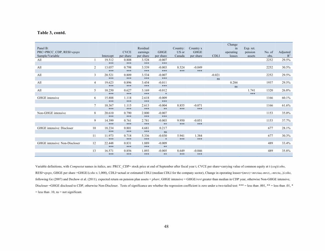
48
Table 3, contd.
Panel B: PRC=PRCC_CDP, RESI=epspx Sample/Variable
Intercept
CVCE per share
Residual earnings
per share GHGE
per share
Country: US or
Canada
Country x GHGE
per share CDLI
Change in
operating leases
Exp. ret. pension
assets No. of
obs. Adjusted
R2 All 1 19.512 0.808 3.528 -0.007
2252 29.5%
*** *** *** *** All 2 13.057 0.798 3.539 -0.003 8.524 -0.049
2252 30.5%
*** *** *** *** *** *** All 3 20.521 0.809 3.534 -0.007
-0.021
2252 29.5%
*** *** *** ***
ns All 4 19.623 0.896 3.454 -0.011 0.284 1937 29.5%
*** *** *** *** ns All 5 10.250 0.627 3.169 -0.012
1.741 1320 26.8%
*** *** *** *
*** GHGE intensive 6 15.888 1.118 2.618 -0.009
1166 60.1%
*** *** *** *** 7 10.367 1.115 2.613 -0.004 8.855 -0.071
1166 61.6%
*** *** *** ** *** *** Non-GHGE intensive 8 20.610 0.790 2.800 -0.007
1153 35.0%
*** *** *** *** 9 14.399 0.761 2.781 -0.003 9.950 -0.051
1153 37.7%
*** *** *** ** *** *** GHGE intensive: Discloser 10 18.234 0.801 4.681 0.217
677 28.1%
*** *** *** ns 11 11.973 0.718 5.336 -0.030 5.941 1.384
677 30.3%
*** *** *** * *** *** GHGE intensive: Non-Discloser 12 22.448 0.831 1.889 -0.009
489 33.4%
*** *** *** ** 13 16.571 0.856 1.893 -0.005 8.649 -0.046
489 35.8%
*** *** *** ** *** ***
Variable definitions, with Compustat names in italics, are: PRCC_CDP= stock price at end of September after fiscal year t, CVCE per share=carrying value of common equity at t (ceq)/csho,
RESI=epspx, GHGE per share =GHGE/(csho x 1,000), CDLI=actual or estimated CDLI (median CDLI for the company sector), Change in operating leases=(mrctt+mrctaat-mrctt-1-mrctat-1)/csho,
following Ge (2007) and Dechow et al. (2011), expected return on pension plan assets = pbarr, GHGE intensive = GHGE/revt greater than median in CDP year, otherwise Non-GHGE intensive,
Discloser =GHGE disclosed to CDP, otherwise Non-Discloser. Tests of significance are whether the regression coefficient is zero under a two-tailed test: *** = less than .001, ** = less than .01, *
= less than .10, ns = not significant.

49
Table 4: Event study of investor response to climate change news Panel A: Investor response around event days -10 to 10: Unsigned excess return and adjusted volume: All 8-K observations
Variable Mean unsigned excess return Mean adjusted volume Mean unsigned excess return Mean adjusted volume Partition 8-K 8-K and PR Sig. 8-K 8-K and PR Sig. First 8-K Subsequent Sig. First 8-K Subsequent Sig.
Event day -10 0.0143 0.0184 *** 8.4511 11.2796 *** 0.0180 0.0178 ns 11.1174 10.8563 ns
-9 0.0134 0.0183 *** 8.3906 11.2198 *** 0.0195 0.0172 * 10.3386 10.9875 ns -8 0.0159 0.0193 ** 8.8030 10.7134 ** 0.0180 0.0191 ns 10.6348 10.4170 ns -7 0.0150 0.0197 *** 8.7299 10.9599 ** 0.0194 0.0190 ns 10.2905 10.7695 ns -6 0.0153 0.0201 *** 8.7748 10.9973 ** 0.0207 0.0192 * 10.6749 10.7173 ns -5 0.0133 0.0192 *** 8.1633 11.1575 *** 0.0187 0.0184 ns 10.9310 10.7225 ns -4 0.0146 0.0197 *** 8.2786 11.0375 *** 0.0205 0.0186 * 11.0864 10.5664 ns -3 0.0159 0.0190 ** 8.7494 11.1762 *** 0.0187 0.0186 ns 11.0278 10.8138 ns -2 0.0139 0.0209 *** 9.0387 11.3998 ** 0.0197 0.0201 ns 10.5923 11.2239 ns -1 0.0177 0.0213 ** 10.1134 12.3575 ** 0.0208 0.0209 ns 12.0742 12.0648 ns 0 0.0199 0.0275 *** 11.2913 15.4774 *** 0.0272 0.0264 ns 14.9109 14.9227 ns 1 0.0174 0.0234 *** 10.1728 13.8325 *** 0.0236 0.0224 ns 13.3430 13.3556 ns 2 0.0155 0.0209 *** 10.0642 12.7999 ** 0.0213 0.0199 * 12.6487 12.3858 ns 3 0.0170 0.0196 * 9.3266 11.9565 *** 0.0204 0.0189 * 12.2209 11.4432 ns 4 0.0160 0.0194 ** 8.5395 11.7785 *** 0.0201 0.0187 * 11.7286 11.2499 ns 5 0.0145 0.0189 *** 8.6591 11.8684 *** 0.0192 0.0181 ns 12.0495 11.2849 ns 6 0.0145 0.0187 *** 8.8438 11.4840 *** 0.0189 0.0179 ns 11.1252 11.1402 ns 7 0.0144 0.0191 *** 8.5886 11.5201 *** 0.0185 0.0185 ns 11.4303 11.0575 ns 8 0.0148 0.0188 *** 8.8829 11.4317 *** 0.0189 0.0181 ns 11.6027 10.9633 ns 9 0.0160 0.0187 * 9.1156 11.5880 ** 0.0178 0.0185 ns 11.7461 11.1301 ns
10 0.0151 0.0190 ** 11.5568 8.4401 *** 0.0196 0.0182 * 10.9513 11.2031 ns Sig. t=0 ** *** ** *** *** *** *** ***
Variable definitions. Unsigned excess return=absolute value of daily stock return inclusive of dividends for trading day t in
excess of the day t return on the CRSP value-weighted market index, adjusted volume=reported trading volume divided by
common shares outstanding at day t (times 50 percent for a NASDAQ company, 8-K=climate change disclosure on filing
date (day 0), 8-K and PR=press release accompanies 8-K filing, Company’s first 8-K filing in fiscal year, otherwise
subsequent. Tests of significance are whether the difference in the mean of the two preceding columns is zero under a
two-tailed test: *** = less than .001, ** = less than .01, * = less than .10, ns = not significant. The last row tests whether
the mean for each column at t=0 differs from the mean on the other days.

50
Table 4, contd. Panel B: Investor response around event days 0 and -1 to 1: Unsigned excess return and adjusted volume
Response variable (cols.) Event day 0
Event days -1 to 1
Event day 0: EARN=1
Event day 0: EARN=0
Section 1: Unsigned excess return Coeff. x 100 Sig. Coeff. x 100 Sig. Coeff. x 100 Sig. Coeff. x 100 Sig. Intercept 1.9479 *** 1.9277 *** 3.6161 *** 1.1747 * EARN 0.0386 ns 0.0386 ns GHGI 0.0703 * 0.0703 * -0.0748 ns 0.1245 *** SIZE -0.0444 * -0.0444 * -0.1121 ** -0.0110 ns CDLI 0.0081 *** 0.0081 *** 0.0055 * 0.0080 *** USAC -0.5026 *** -0.5026 *** -0.3195 ns -0.5255 *** DSLC -0.3958 *** -0.3958 *** -0.5018 *** -0.3564 *** RISK 0.8184 *** 0.8184 *** 0.8497 *** 0.7860 *** EVTD 0.8680 *** 0.4316 *** 1.8459 *** 0.5565 *** EVTD x EARN 1.2827 *** 0.6167 *** EVTD x GHGI -0.4750 ** -0.2079 * -1.3129 *** -0.2719 ns EVTD x SIZE -0.0408 ns 0.0339 ns -0.4499 * 0.0639 ns EVTD x CDLI -0.0154 *** -0.0036 ns -0.0705 *** -0.0020 ns EVTD x USAC -1.6900 *** -0.6559 * 1.2487 ns -2.1495 *** EVTD x DSCL 0.1178 ns -0.0795 ns 0.9222 * -0.1675 ns Adjusted R2 10.3% 9.6% 17.6% 7.7% F statistic 101.41 *** 93.51 *** 53.77 *** 65.29 *** No. of obs. 12,241 12,241 2,959 9,282 Section 2: Adjusted volume Coeff. Sig. Coeff. Sig. Coeff. Sig. Coeff. Sig. Intercept 15.3377 *** 15.210 *** -16.291 ns 19.338 *** EARN 0.6256 ** 0.626 ** GHGI 0.4767 * 0.477 * 1.330 * 0.3204 ns SIZE -1.1736 *** -1.174 *** 0.121 ns -1.1917 *** CDLI 0.0760 *** 0.076 *** 0.055 ** 0.0808 *** USAC 9.0528 *** 9.053 *** 7.375 *** 8.4897 *** DSLC -4.1430 *** -4.143 *** -6.218 *** -4.5589 *** RISK 13.8121 *** 13.812 *** 19.501 *** 10.6696 *** EVTD 4.1199 *** 2.270 *** 9.627 *** 2.3653 *** EVTD x EARN 7.0036 *** 2.906 *** EVTD x GHGI -3.0331 ** -1.233 * -9.596 *** -1.0106 ns EVTD x SIZE -0.1047 ns -0.186 ns 0.7246 ns EVTD x CDLI -0.0725 * -0.025 ns -0.309 *** -0.0241 ns EVTD x USAC 1.8894 ns 0.261 ns 11.191 ns 0.6088 ns EVTD x DSCL 0.4532 ns -0.432 ns 2.878 ns -0.2020 ns Adjusted R2 35.0% 34.8% 50.1% 26.6% F statistic 471.74 *** 466.81 *** 55.42 *** 281.92 *** No. of obs. 12,241 12,241 2,959 9,282
Variable definitions. Dependent variable = daily unsigned excess return or adjusted volume for given event day window, EARN = 1 if
earnings information in 8-K, otherwise 0, GHGI = 1 if GHGE/revt in CDP year greater than median, otherwise 0, SIZE = log of at for
prior fiscal year, CDLI = 1 if actual or estimated CDP Disclosure Leadership Index in CDP year greater than sample median, otherwise 0,
USAC = 1 if USA, otherwise Canada, DSCL=1 if GHGE disclosed to CDP, otherwise 0, RISK = CRSP beta, EVTD = 1 for event days
in event window, otherwise 0. Tests of significance are whether the regression coefficient is zero under a two-tailed test: *** = less
than .001, ** = less than .01, * = less than .10, ns = not significant.

51
Table 4, contd.
Panel C: Investor response to climate change news around event days -10 to 10: Signed excess return Mean Cumulative mean Standard deviation
Event day
Low GHGE
intensity
High GHGE
intensity
Mean Difference Mean Sig,
Low GHGE
intensity
High GHGE
intensity
Cum. mean Difference Mean Sig,
Low GHGE
intensity
High GHGE
intensity -10 0.041% 0.184% 0.143% ns 0.041% 0.184% 0.143% ns 2.910% 2.614%
-9 -0.278% 0.091% 0.369% ns -0.236% 0.275% 0.512% ns 2.670% 2.435% -8 0.324% -0.048% -0.372% * 0.088% 0.228% 0.139% ns 3.201% 2.226% -7 0.049% 0.021% -0.027% ns 0.137% 0.249% 0.112% ns 3.487% 2.175% -6 -0.076% 0.048% 0.124% ns 0.061% 0.297% 0.236% * 3.154% 3.765% -5 0.264% -0.003% -0.267% * 0.325% 0.294% -0.031% * 2.887% 2.179% -4 0.248% -0.146% -0.394% * 0.573% 0.148% -0.425% * 3.470% 2.829% -3 0.227% -0.076% -0.303% * 0.800% 0.072% -0.728% * 3.012% 2.171% -2 0.030% -0.140% -0.170% ns 0.830% -0.068% -0.898% ** 3.012% 2.245% -1 0.185% 0.060% -0.125% ns 1.016% -0.008% -1.024% * 3.528% 2.883% 0 -0.229% -0.127% 0.103% ns 0.786% -0.135% -0.921% * 5.489% 3.461% 1 -0.111% -0.079% 0.032% ns 0.675% -0.214% -0.889% * 4.096% 3.022% 2 0.013% 0.151% 0.138% ns 0.688% -0.062% -0.751% ns 3.040% 2.260% 3 0.197% 0.069% -0.128% ns 0.885% 0.006% -0.879% ns 2.944% 2.053% 4 0.134% 0.020% -0.114% ns 1.019% 0.027% -0.992% * 3.021% 2.311% 5 -0.015% 0.211% 0.226% ns 1.003% 0.237% -0.766% ns 2.531% 2.239% 6 -0.151% 0.273% 0.423% ns 0.853% 0.510% -0.343% ns 2.837% 2.548% 7 0.211% 0.042% -0.169% ns 1.064% 0.552% -0.512% ns 3.161% 2.246% 8 0.047% 0.106% 0.059% ns 1.111% 0.658% -0.453% ns 2.968% 2.115% 9 -0.137% 0.045% 0.182% ns 0.974% 0.703% -0.271% ns 2.817% 2.112%
10 -0.032% -0.229% -0.197% ns 0.942% 0.474% -0.468% ns 3.350% 2.155%
Variable definitions. Signed excess return = daily stock return inclusive of dividends for trading day t in excess of the day
t return on the CRSP value-weighted market index, Event day = climate change disclosure relative to 8-K filing date,
High GHGE intensity = GHGE/(revt*1000) greater than median in CDP year, otherwise low GHGE intensity. Standard
deviation = standard deviation of signed excess return for event day t. Tests of significance are whether the mean
difference is zero under a two-tailed test: *** = less than .001, ** = less than .01, * = less than .10, ns = not significant.

52
Table 5: Regression of stock price on common equity, residual earnings, and GHG emissions per share with selection equation
Dependent variable: Stock price = PRCC_Q5 Regr. 1 in panel A of table 3 Regr. 2 in panel A Regr. 3 in panel A Regr. 4 in panel A Regr. 5 in panel A Second-stage valuation regression Coef. Signif. Coef. Signif. Coef. Signif. Coef. Signif. Coef. Signif. Intercept 21.211 *** 18.160 *** 25.968 *** 23.259 *** -3.647 ns CVCE per share 0.627 *** 0.633 *** 0.633 *** 0.666 *** 0.625 *** Residual earnings per share 3.209 *** 3.229 *** 3.212 *** 3.207 *** 3.066 *** GHGE per share -0.011 *** -0.008 * -0.011 *** -0.010 * -0.030 ** Country 3.301 * Country*GHGE per share -0.014 ns CDLI -0.070 * Change in operating leases -1.078 ns Exp. Ret. pension assets 3.474 *** Inverse Mills ratio (IMR) 0.773 ns 1.135 ns -0.099 ns -0.641 ns -0.410 ns First-stage selection equation Sector (same as table 2) Yes Yes Yes Yes Yes Book-to-market ratio 0.005 ns 0.005 ns 0.005 ns 0.009 ns -0.009 ns Long-term debt to total assets -0.587 *** -0.587 *** -0.587 *** -0.680 *** -0.549 *** Previous discloser 0.510 *** 0.510 *** 0.510 *** 0.571 *** 0.448 *** Other channel 1.131 *** 1.131 *** 1.131 *** 0.948 *** 1.212 *** Intercept -0.387 *** -0.387 *** -0.387 *** -1.572 *** -0.402 *** No. of observations in valuation regression1 2,309 2,309 2,309 1,989 1,353 No. of CDP discloser observations in selection equation 970 970 970 809 683 Wald Chi Square 608.68 615.00 614.09 556.19 434.04 Average VIF of regressing IMR on independent variables in the second-stage valuation regression
1.21 1.20 1.16 1.29 1.13
Variable definitions, with Compustat names in italics, are: PRCC_Q5=stock price at end of first quarter after fiscal year t, CVCE per share=carrying value of common equity at t (ceq)/csho,
RESI=epspx, GHGE per share=GHGE/(csho x 1,000), CDLI=actual or estimated CDLI (median CDLI for the company sector), Change in operating leases=(mrctt+mrctaat-mrctt-1-mrctat-1)/csho,
following Ge (2007) and Dechow et al. (2011), expected return on pension plan assets=pbarr, GHGE intensive=company in GHG intensive sector based on GHG/revt, otherwise company in non-
GHGE sector, Discloser=GHGE disclosed to CDP, otherwise Non-Discloser. Tests of significance are whether the regression coefficient is zero under a two-tailed test: *** = less than .001, ** =
less than .01, * = less than .10, ns = not significant.
1. The number of observations is less than in table 3 because we require that we have no missing observations for both the selection equation and the valuation regression.

53
Table 6: Economic significance of GHGE regression coefficients
Variable Table 3 model 1 Table 5 model 1 Calculation Data item (1) (2) (3) (4) GHGE market price per ton 1 $20.00 $7.00 $20.00 $9.96 GHGE/(csho*1000) regression coefficient 2 -0.0075 -0.0075 -0.0106 -0.0106 GHGE/(csho*1000), median 3 1.3725 1.3725 1.3725 1.3725 GHGE per share times -1 4 = -2 x 3 0.0103 0.0103 0.0146 0.0146 GHGE median, in tons 5 327,237 327,237 327,237 327,237 Number of shares outstanding, median 6 223,000,000 223,000,000 223,000,000 223,000,000 GHGE per share 7 = 1 x 5 ÷ 6 0.0293 0.0103 0.0293 0.0146 GHGE cost ratio 4 ÷ 7 35.00% 100% 49.76% 100%
This table calculates the GHGE cost ratio, where the cost ratio equals GHGE per share for the median company implied by regression model 1 in
table 3 or table 5 divided by GHGE per share for the median company in the sample. As such, the numerator represents investors’ assessment of
the impact of GHGE per share on stock price and the denominator represents total GHGE per share priced at an assumed market price per ton. For
example, at a cost of $20 per ton, investors factor 35% of that cost into stock price as an unrecognized liability (calculation 1). Equivalently,
investors factor an unrecognized liability of $7.00 per ton of GHGE into stock price (calculation 2), conditional on the regression model. Variable
definitions, with Compustat name in italics, are: GHGE/(csho*1000) =GHGE per common share; median = median over all sample
observations.