Scheduling Techniques to Classify Wear Particles on...

Scheduling Techniques to Classify Wear Particles on Multi-Computers

Mohammad Shakeel Laghari1 & Gulzar Ali Khuwaja2 1Department of Electrical Engineering

UAE University, Al Ain, United Arab Emirates 2Department of Computer Engineering

King Faisal University, Al Ahsa, Kingdom of Saudi Arabia [email protected], [email protected]

ABSTRACT Processor scheduling techniques are used in conjunction to exploit the major paradigms of algorithmic parallelism, geometric parallelism, and processor farming. Static process scheduling techniques are successfully used with algorithmic and geometric parallelism, whilst dynamic process scheduling is better suited in dealing with the independent processes inherent in the processor farming paradigm. This paper investigates the application of parallel, or multi-computers to a class of problems exhibiting spatial data characteristic of the geometric paradigm that is best suited to the static scheduling scheme. However, by using the processor farming paradigm, a dynamic scheduling technique is developed to suit the MIMD structure of the multi-computers. The specific problem chosen for the investigation is the recognition and classification of microscopic wear particles generated by wear mechanisms. Experiments are performed on both schemes and compared in terms of total processing time, speedup, and efficiency. KEYWORDS Classification, computer vision, parallel processing, recognition, scheduling, wear particles. 1 INTRODUCTION Computer vision and image processing are sometimes considered as a field of applied artificial intelligence concerned

with computer processing of images from the real world. It typically requires a combination of low-level image processing to enhance the image quality, higher-level pattern recognition, and image understanding to recognize features present in the image. It is also a process to locate and recognize objects in digital images. Computer vision has been used in diverse areas of applications. One such important area is in the field of on-line or off-line visual inspection systems of microscopic applications. These applications also have a potential to be decomposed into processes to exploit inherent parallelism. To exhibit this parallelism, the most commonly used parallel paradigms in scientific applications are algorithmic parallelism, geometric parallelism, and processor farming [1], [2], [3]. Processor scheduling determines which and when processes are assigned to specific processors. There are different techniques of processor scheduling that can be used to optimize performance in parallel computer systems. Static process scheduling is defined for a given sets of tasks, a mapping of processes to processors before the execution of the processes. This scheduling technique is used successfully to exploit algorithmic and geometric parallelism. Whilst in dynamic process scheduling, mapping of processes to processors is delayed until the processes are executing and is better

52

International Journal of New Computer Architectures and their Applications (IJNCAA) 3(1): 52-71 The Society of Digital Information and Wireless Communications (SDIWC) 2013 (ISSN: 2220-9085)

suited to dealing with the independent processes inherent in the process farming paradigm [4], [5], [6]. Processors in operation generally perform two functions: computations and communications. A suitable balance between these functions is required to ensure efficient use of the processing resources. However, when the time taken to perform the computation of a given sub-problem is less than the time associated with the communications of the data and results, then the communication bandwidth is likely to limit the performance. An appropriate scheduling technique can keep the processors utmost engaged and help achieve optimum performance. The location and recognition of objects in digital images is an important aspect of computer vision. An important feature of this application is in the automation of visual inspection systems, which enables the manufacturing industry to improve its quality, productivity, and economy. These inspection techniques also apply to the automatic analysis of microscopic images. The problem chosen in such microscopic applications is the classification and recognition of wear particles generated by wear mechanisms in a mechanical system [7], [8], [9], [10]. The work presented in this paper investigates the performance of scheduling techniques for the parallel implementation of grid-type applications implemented on a MIMD machine. Several algorithms are developed for this application, and are executed on a Networked Processor Linear Array (NPLA). Experiments are performed and compared in terms of total processing times, speedup, and efficiency, by using a varying number of processors and computational load.

2 REVIEW OF PARALLEL PROCESSING Since their invention in the 1940's, computers based on the John von Neumann architecture have been built around one basic plan; a single processor, connected to a single store of memory, executing one instruction at a time. The processor fetches instructions from a program stored in the memory, decodes the instruction, fetches operands for these instructions, performs calculations, and then writes the results back to the memory. The von Neumann architecture was popular for several reasons. It was conceptually simple; von Neumann machines were economical and simple to build. The idea of parallelism was introduced at the same era by von Neumann to use multiple processors to solve a single problem. The aim was to build a cellular automata machine in which a very large number of simple calculators work simultaneously on the small parts of a larger problem. However, the idea did not gain reality because of the limited hardware and software capabilities of that time. Things changed in 1960's when vacuum tubes were replaced by solid-state components. Instead of using one arithmetic & logic unit, multiple (replicated) functional units were incorporated in a machine resulting in the CDC 6600 computer, which was a state-of-the-art machine of that time operating at a clock speed of 100 nanoseconds. The first vector computer called Cray 1 was developed in the early 1970's. This vector computer was based on overlapping of operations. In vector computers, the arithmetic & logic unit is divided into stages. If two long vectors

53


of numbers, are being added together, successive additions are overlapped to increase the overall throughput. In the late 1970's, four developments in the field made parallel processing a reality. The first was the development of the VLSI (Very Large Scale Integration) technology, which allowed hundreds of thousands of transistors to be integrated on a single integrated circuit. The second was in the development of better concurrent programming methods. The third was the actual construction of parallel computers. C.mmp (Computer with multiple mini-processors) from Carnegie-Mellon University is one such example of parallel computers. Lastly, the continued development in the field of high speed vector computers. By the early 1980s, parallel computers were being manufactured commercially. The main advantage was the cost, since most parallel computers at that time were economical compared to their serial counterparts. Nevertheless, the speed of light limited the performance of parallel computers. Therefore, the way of performing computations more quickly is to move more bits of data at once, which is referred to as parallelism. These computers contain several processors together in order to solve a single problem. The question remains on how many processors should be used, how big they should be, and how should they be organized and scheduled? Multiple processor systems have a number of potential disadvantages, probably the most prominent being the very real problem of being able to use the processing power efficiently. For example, if a processor solves a problem in some specific time, then it is unlikely to solve the same problem in exactly half the time when two processors are used. This involves a number of factors; the

ability to decompose a problem into an optimum number and size of modules, and to define these modules in such a way that communications between processors may be carried out with the absolute minimum waiting time and a minimal delay, across the communication network. Successive knowledge has also shown that building parallel hardware is less difficult than providing attractive parallel software tools, to utilize the hardware efficiently [11]. This is because unlike the von Neumann model for sequential computing, there is no general-purpose model for parallel computation [12]. There is no single computation model that can guide the choices of parallel programmers in designing, implementing, and evaluating the performance of parallel software. Consequently, a program decomposition that is efficient on one parallel machine might become inefficient on another parallel machine. Real time problems in current times tend to involve a large amount of data received at varying times and rates, and yet responses are required to be generated instantly. To create a system, which is very general, and yet provides maximum efficiency, poses great complications. 3 CLASSIFICATION OF COMPUTERS Computer systems are classified into a number of collective groups determined by the type of processing which is required, together with the method by which the processing elements communicate, use memory, and operate with efficiency. All computer systems, sequential and parallel, are divided according to the following schemes:

54


Feng's Scheme: This scheme is based on serial versus parallel processing. Handler's Classification: This classification is determined by the degree of parallelism and pipelining at various subsystem levels. Shore's Taxonomy: This taxonomy is based on how the computer is organized from its constituent parts (six machines). Skillicorn's Taxonomy: This is based on the functional structure of the architecture, and the data flow between its component parts. Flynn’s Classification: This classification is based on the multiplicity of instruction streams and data streams in a computer system. Most of the serial and parallel computers are classified according to this taxonomy, thus, it is discussed in detail. Four schemes of Flynn's classification are: 3.1 SISD (single instruction stream / single data stream) This is the conventional serial John von Neumann computer, as shown in Figure 1a. Most serial computers fall into this category. Although instruction execution is pipelined, computers in this category can decode only a single instruction in unit time. A SISD computer may have multiple functional units, but are under the direction of a single control unit. The abbreviations used in the Figure are PM (program memory), IS (instruction stream), CU (control unit), PU (processing unit), MM (memory module), & DS (data stream). 3.2 SIMD (single instruction stream /

multiple data streams) These computers involve multiple processors simultaneously executing the

same instruction on different data. These are the systems with multiple arithmetic-logic processors, or units and a control processor, as shown in Figure 1b. Each arithmetic-logic unit processes a data stream of its own, as directed by the single control unit. SIMD machines are also called array processors. SIMD specifies a style of processing which operates on vectors of data. All execution units are synchronized and operate in lock step in response to instructions from a single instruction stream and suitable for low-level image processing tasks. SIMD models differentiate based on memory distribution and addressing scheme used. Most SIMD computers use a single control unit and distributed memories, except for a few that use associative memories. 3.3 MISD (multiple instruction

streams / single data stream) These computers involve multiple processors applying different instructions to a single data stream. There are few machines in this category, but none has been commercially realized. One type of system that fits the description of an MISD computer is a systolic array, which is a network of small computing elements connected in a regular grid. 3.4 MIMD (multiple instruction

streams / multiple data streams) This consists of processing elements linked by an interconnection network, or by accessing data in shared memory units. Each processing element stores and executes independent instruction streams, using local data as shown in Figure 1c. MIMD computers support

55


parallel solutions that require processors to operate in a largely autonomous manner. Thus, MIMD architectures are asynchronous computers, characterized by decentralized hardware control. These architectures are suitable for higher-level image analysis and computer vision operations [13].

Figure 1a. SISD computer.

Figure 1b. SIMD computer.

Figure 1c. MIMD computer. With the aid of Flynn's classification, a structural taxonomy of both serial and parallel computers is formulated. A basic division is made according to the instruction streams. The single instruction computers consist of SISD and SIMD machines. The SISD computers include single-unit serials, multiple-unit scalars, and pipelined

computers. The SIMD computers include processor arrays and associative processors. In the multiple instruction streams, the MIMD architectures are divided into subgroups of multiprocessors and multi-computers. The multiprocessors are classified in terms of loosely coupled, which is sharing the local memory of the processors, and tightly coupled, which is that all the processors share a global memory through a central switching mechanism. Multi-computers are characterized by distributed memory. Every CPU has its own memory, and all communications (point-to-point) and synchronization between processors are via message passing. Distributed memory multiprocessors are characterized by their network topologies. Parallel systems based on geometrical decomposition of applications are divided into three categories of computer based dedicated systems; computer based general systems, and digital signal processing systems. The first category includes array processor, pipeline computers, multiprocessor systems, very large scale integration, whereas the second one includes Distributed Shared Memory (DSM), Massive Parallel Processing (MPP), & Clusters, and the third one shares the combined capabilities of the first two categories [14], [15], [16], [17]. 4 PARALLEL PARADIGMS In order To efficiently utilize the computational potential of a large number of processors in a parallel system, it is necessary to identify the important parallel features of the application. There are three common paradigms for exploiting parallelism in

56


scientific and engineering applications. Essentially, these paradigms are based on different approaches to problem decomposition. The paradigms fall into the following classes. 4.1 Algorithmic Parallelism Algorithmic parallelism is present where the algorithm can be broken down into a pipeline of processors in such a way that each processor executes a small part of the total algorithm. The parallelism inherent in the algorithm is exploited. In this decomposition, the data flows through the processing elements and is sometimes referred to as Data Flow parallelism. The communication loads on each processor are increased when the data is passed and the communication bandwidth problems can degrade the performance. For algorithmic parallelism to be successful, the workload must be balanced uniformly across the processors. However, with an imbalanced workload it is unlikely to offer a speedup, which is proportional to the number of the processors used. This is due the fact that the throughput of a pipeline is limited by the throughput of the slowest element within it. The advantage of this decomposition is that modest memory is required per processor. The computer systems based on the algorithmic parallelism give acceptable efficiency. Figure 2 shows an example of algorithmic parallelism in terms of a language compiler. 4.2 Geometric Parallelism Geometric parallelism utilizes the underlying geometric structure of the particular problem under consideration. The method enables to make use of

inherent data parallelism of a large class of grid problems. This is present where the problem can be broken down into a number of similar processes in such a way as to preserve processor data locality and each processor operate on different subset of the total data to be processed. All the data required by a processor is arranged to be on that processor, or one of its immediate neighbors. As this type of parallelism requires only a fraction of the total data on each processor, therefore, it is sometimes called as Data Structure parallelism. Figure 2. Example of algorithmic parallelism – a

language compiler. In the geometric decomposition, immediate neighboring processors communicate with each other. The communication loads are proportional to the size of the boundary of the element, while the computational loads are proportional to the volume of the element. Each processor has an almost complete copy of the whole program, therefore moderate memory requirements. The computer systems based on the geometric parallelism offers very good efficiency. Geometric decomposition works for both, fine grain and median grain problems. The larger the sub-region placed on a node, the greater the ratio of bulk compotation to surface communication and hence the higher efficiency. Figure 3 shows an example of data structure parallelism.

lexer parserSource

Machinecode

semantic analyzer I.R. code generator

code generatoroptimizer

57


Figure 3. Example of geometric structure. 4.3 Processor Farming This is one of the simplest methods of exploiting parallelism. Processor farming consists of a farmer processor, that distributes independent tasks of work to a set of worker processors and receive back the results. It is often most efficient to run these independent tasks concurrently on different processors. The typical architecture for these types of applications is a farm of processors where each processor is executing the same program with different initial data in isolation from all the other processors. The memory requirement is more, compared to the other paradigms. Due to the very limited communication requirements because of independent tasks, this method is very efficient, but the memory costs may be significant higher [18], [19].

Figure 4 shows an example of processor farming paradigm. In general, a master processor distributes independent tasks to a pool of slave processors, where actual computation takes place. Various topologies (linear chain, ternary tree, etc.) may be used for the farming networks and the most efficient one for any given application depends on the precise hardware characteristics of the farming processors.

Figure 4. Example of processor farm. 5 WEAR PARTICLES The term Wear Particle or Wear Debris relates from the field of “Tribology”. It is the study of wear, friction, and lubrication. The concept was first enunciated in 1966 by the British Department of Education and Science [20]. All mechanical systems contain moving parts, come in contact when the machine is operated. Wear particles are produced with interactions between surfaces and more specifically the removal and deformation of material on a surface because of mechanical action of the opposite surface. After the initial run period of any machine, which regularly generates large amount of wear particles, a steady state in the machine operation is reached to produce a relatively less or normal amount. A machine in such a steady state is said to be operating under normal wear mechanism. Any change in the steady state generates a change in the normal wear mechanism. This change in the microscopic wear particles transported by a lubricant from wear sites carry with them important information relating to the condition of engines and other machinery [21]. Particles are separated from the lubricant (oil) and are placed onto slides for examination and analysis. Experts in the fields (Tribologists) examine these prepared slide samples by using an optical or scanning electron microscope. The samples provide a wealth of information on the wear processes

58


involved and on the state of the machinery. Particles contained in the lubricant can be separated for off-line examination by using several methods: • Different sizes of filters are used at

specific locations in machines to separate particles from the lubricating oil, and are deposited on glass slides for examination and analysis.

• The name, Ferrography, derives from the initial development of the methods to precipitate ferrous wear particles from engine lubricating oil. Ferrography is another technique in which particles are separated and arranged according to their relative size on a transparent substrate. It is also commonly used for determining or measuring wear of machine systems. The determination of at least one of quantity, size, type, surface features of wear particles provides an indication of the wear status of the machine system. The particles size is typically between ranges of 1 to 100 µm [22].

• The magnetic chip detectors or MCD is a typical method used for collecting ferrous wear particles from samples. Magnetic plugs are small removable units fitted with a powerful permanent magnet, and are located at convenient positions in the machine. Typically, large sized particles (larger than 100 microns) stick to the plug, and then the plug is wiped on a slide for quantitative and qualitative analysis [23].

There are other on-line and off-line systems, in which abnormal wear modes are detected: • In an on-line detection system,

transparent tubes are located at convenient positions in the machine through which lubricant is passed. Tribologists perform timely visual

checks of the passing lubricant for the particle concentration.

• Spectroscopic analysis is an off-line method in which the lubricant sample containing wear particles is diluted and aspirated into an energy source, which excites wear metals within the lubricant sample such that the wear metals give off optical emissions at visible wavelengths. The optical emissions can be registered and analyzed for determining size and quantity of the wear metals within the lubricant sample, and accordingly measuring the wear of the machine system. This method is generally used to detect particles lesser than 10 microns [24].

The opportunities available for capturing wear particles are illustrated in Figure 5.

Figure 5. Opportunities for capturing wear debris.

Wear particles are classified in two ways; quantitative method and morphological analysis. Quantitative is an old and the most commonly utilized method for monitoring wear. This method of measurement is objective and quick, as it only considers particle size and quantity. Wear particle size distribution is useful in detecting significant transitions in the wear activity and could provide early indications of impending failure. The ability to identify an increase in particle size can give an indication of caution. In fact, early monitoring was dependent on the parameters of size and quantity only.

oil filteroil sample

magnetic plugoff-line measurement & analysis

on-linemeasurement

f

59


X-ray fluorescence analysis (XRF) is a powerful tool for elemental analysis of structural metals, and is suitable for determining wear metal quantity, elemental composition, production rates for each element, and wear sources. However, experience of using this method alone, and in isolated situations, has resulted in confusion about the information it yields and hence, reliability is questionable [25]. Morphological analysis is performed off-line by using an optical microscope. Studying particle morphology reveals information about the condition of the machine. It is commonly used to detect abnormal wear modes. Detailed examination is required to collect specific information about the condition of the moving surfaces of the machines’ elements. Considerable time and experience is required if reliable determination is to be made about the wear state, and source of the wear. Morphological analysis not only identifies wear failures, but also the specific part of the machine causing it [26]. Six morphological attributes have been identified as particle size, shape, edge detail, color, thickness ratio, and texture. Experts in the field characterize the particles with particular morphology, and relate these to known wear modes. This type of analysis yields specific information about the condition of the moving surfaces of the machines’ elements from which they are produced, the mechanism of their formation, and the mode of wear in operation in the system from which they are extracted [27], [28], [29], [30]. Particles generated by different wear mechanisms have characteristics, which can be identified with the specific wear mechanism. The relationship between

the wear particle properties and the condition under which they are formed enables particles to be classified in a number of types. Each particle type gives a different clue about the machine condition and performance. Current research in the field has suggested 29 different types of wear particles. A few examples of wear particle descriptions are [31], [32], [33]: • Rubbing wear: This particle type is

formed by the normal sliding of a metal surface against another metal, or by exfoliation of parts of the shear mixed layers. This wear is of benign nature and frequently referred to as an acceptable normal rubbing wear. These particles consists of flat platelets, generally 5 microns or smaller in size. There is no visible texturing of the surface and the thickness is one micron or less. No immediate action is required in normal circumstances.

• Cutting wear: This particle type is generated because of one surface penetration, plough, or cutting another surface. A relatively hard component can become misaligned or fractured, resulting in hard sharp edge penetrating a softer surface. It takes the form of spirals, loops, and long bent wires averaging 2 to 5 microns wide and 25 microns to 100 microns long. Cutting wear particles are abnormal. Their presence and quantity is carefully monitored. If a system shows increased quantities of large (50 microns long) cutting wear particles, a component failure is potentially imminent.

• Severe sliding wear: This particle type is formed under the conditions of excessive surface loading, increased running speed, or poor lubrication. These particles have distinct surface features of parallel striation marks and are generally larger than 15

60


microns, with the length-to-width thickness ratio falling between 5 and 30 microns. The presence of such particles is an indicative of active wear process and requires careful monitoring, and sometimes need immediate action.

• Chunky Fatigue, Laminar Rolling Fatigue, Spherical, Oxide, Bearing Wear, Gear Wear, etc. are few other examples of wear particles.

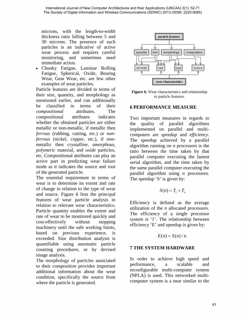
Particle features are divided in terms of their size, quantity, and morphology as mentioned earlier, and can additionally be classified in terms of their compositional attributes. The compositional attributes indicates whether the obtained particles are either metallic or non-metallic, if metallic then ferrous (rubbing, cutting, etc.) or non-ferrous (nickel, copper, etc.), if non-metallic then crystalline, amorphous, polymeric material, and oxide particles, etc. Compositional attributes can play an active part in predicting wear failure mode as it indicates the source and root of the generated particle. The essential requirement in terms of wear is to determine its extent and rate of change in relation to the type of wear and source. Figure 6 lists the principal features of wear particle analysis in relation to relevant wear characteristics. Particle quantity enables the extent and rate of wear to be monitored quickly and cost-effectively without stopping machinery until the safe working limits, based on previous experience, is exceeded. Size distribution analysis is quantifiable using automatic particle counting procedures, or by devised image analysis. The morphology of particles associated to their composition provides important additional information about the wear condition, specifically the source from where the particle is generated.

Figure 6. Wear characteristics and relationship

to particle features. 6 PERFORMANCE MEASURE Two important measures in regards to the quality of parallel algorithms implemented on parallel and multi-computers are speedup and efficiency. The speedup achieved by a parallel algorithm running on n processors is the ratio between the time taken by that parallel computer executing the fastest serial algorithm, and the time taken by the same parallel computer executing the parallel algorithm using n processors. The speedup ‘S’ is given by:

nTTnS += 1)( Efficiency is defined as the average utilization of the n allocated processors. The efficiency of a single processor system is ‘1’. The relationship between efficiency ‘E’ and speedup is given by:

nnSnE /)()( =

7 THE SYSTEM HARDWARE In order to achieve high speed and performance, a scalable and reconfigurable multi-computer system (NPLA) is used. This networked multi-computer system is a near similar to the

particle features

size morphologyquantity composition

severity rate

wear characteristics

type source

61


NePA system used to implement Network-on-Chip [34]. The system used is a linear array of processors. It includes RISC processors and memory blocks. Each processor in the array has a compactOR, internal instruction memory, internal data memory, data control unit, and registers. One of the processors is used as a master or main, processor and the remaining as slaves. The system has a network interface with the main processor having four, and others equipped with two, port routers. Routers can transfer both control, as well as application data among processors. 8 PROFILE DATA PROCEDURES Image processing and analysis procedures are designed in conjunction with a multiple window, hierarchal interactive graphics interface that controls the software and hardware environment. Grey scale images of wear particles, as shown in Figure 7a, are transmitted from the field of view in the microscope via a CCD color camera, and stored in the random access memory of the computer. Objects in an image can easily be identified if they occur at different grey levels than the background. Wear particles in an image are also generally of a different intensity than that of the background. Image segmentation can be thought of as the process of separating the object of interest (wear particle) in an image from the background and from other secondary entities. Segmentation is a particularly difficult problem and the success (or not) of any algorithm depends intensely on the image acquisition quality. It is therefore general to perform the segmentation in an

interactive manner, where the immediate results are analyzed and improved through expert supervision and intervention by users. The simplest and most often adopted methods for image segmentation are based on ‘thresholding’. It is used to remove the grey level trends in an image, to make the grey level regions discrete and split into distinct parts. A straightforward to classify each element as an object pixel or as a background pixel is to set a threshold value in the intermediate range between the background and the foreground grey levels, and to consider as a foreground any point smaller or equal to this value. The result of thresholding is represented as a binary image. There are many different techniques that attempt to improve the thresholding algorithm. For instance, if the illumination is not homogeneous throughout the image, finding a single threshold that produces acceptable results may be impossible. In some of these situations, it is possible to find different suitable thresholds for different image regions, thus suggesting the use of adaptive thresholding algorithms. Another important problem is how to select the threshold value appropriately. Although this can be done manually by trial-and-error, it is desirable to have procedures for automatic thresholding selection in many situations. Nevertheless, the automatic techniques are insufficient for the extraction of wear particles from the background, as particle images generally have a varying contrast. Therefore, interactive thresholding is the method by which particle shapes are extracted, as shown in Figure 7b. After thresholding, three different procedures can be used to identify individual particles for analysis.

62


8.1 Manual Process In this procedure, grey scale image of the microscopic wear particles is stored in the computer memory. The image is threshold by setting all the grey levels below a certain level to zero, or above a certain value to a maximum brightness level. The result of any image segmentation is the unique labeling of each particle pixel that lies contained in a specific distinct segment. A more concise technique is to specify the closed contour of each segment. It is necessary to perform contour filling techniques that can label each pixel within a contour as well as contours of all particles in an image [35]. A contour following approach, commonly called as bug following is used. In the segmented image, a conceptual bug starts from the white background to the black particle region indicated by the closed contour. When the bug crosses into black region, it makes a left turn and proceeds to the next pixel. If that pixel is black, the bug turns left again, and if the pixel is pixel crosses to other region meaning white, the bug turns right. This process continues until the bug returns from where it started which results in boundary detection operation of the wear particle image, as shown in Figure 7c. Particles of interest are interactively selected by using the computer cursor. A boundary tracking algorithm based on a crack code method is used which tracks the border from pixel to pixel of a selected wear particle. While the bug is following the contour, it can create a list of the pixel coordinates of each boundary pixel. These perimeter coordinates are stored in the computer memory [36].

Figure 7a. Grey scale image of the wear particles.

Figure 7b. Threshold image of the wear

particles.

Figure 7c. Profile image of the wear particles. 8.2 Modified Process The manual procedure is modified to enhance the quality of the particle image. The procedure is devised for low quality slides, specifically those prepared from the MCDs, where most of the particles are joined together, touching, and are overlapping. It is also suitable for the images where the particle regions are occluded due to the reflection of microscope light. When viewing the particles in reflected light, it sometimes is reflected back in the

63


camera from the smooth and shiny parts of the particle. Cursor buttons are used on the segmented image to interactively mark and separate touching particles, to remove the underneath or hidden of overlapping particles, and to complete the missing regions of a reflected particle image. After modification, boundary detection is performed, and the particles of choice are selected. 8.3 Automatic Process In this procedure, the system automatically selects all the wear particles in the image. This process is suitable for wear particle slides where the particles are evenly scattered in such a way that they are not touching each other or are overlapping. It follows the same procedure of segmenting the grey scale image of the wear particles into white and black regions. The system scans the image, finds a black region, and labels it with a different pixel value by using a region labeling technique. The labeling process identifies which pixels are connected together to form a separate region. The entire image is labeled from ‘1’ to ‘n’ pixel values of the identified particles in such a way that each image region has a single numerical label to identify the region [37]. After labeling, the system again scans the entire image and automatically performs boundary tracking for each particle by using another devised method called chain coding, in which the path from the centers of connected boundary pixels are represented by an eight-element code. The perimeter coordinates in the computer memory. Figure 8 defines a chain code and provides an example of its use [38], [39].

The sequence of elements from the Figure is given as: CHAIN CODE: 00012 33323 54455 76717

Figure 8. Chain code method. The automatic procedure is modified to select particles according to their size. The procedure is also modified to disregard the particles that are partially touching, or are not fully revealed by the image boundary. The automatic procedure on average, takes about 11 seconds to identify approximately 30 particles in an image. The automatic procedure has proved to be too slow, and hence parallelization is introduced to speed up the whole process. The two scheduling methods of static and dynamic schemes are described as follows. 9 PARALLEL IMPLEMENTATION The two scheduling schemes of static and dynamic are investigated for the automatic procedure. The algorithms are executed on nine processors, of which a linear array of seven processors constitutes the processing elements. The remaining two are used for connection to the local host, and graphics display. One

1

0

76

5

32

64


of the seven processors is the driver or master, which interacts with the user through the local host, directs the operation of the graphics processor, and the remainder of the processing elements collectively known as slaves or workers. The processing elements are connected by a bidirectional communication system, allowing data and results to be transferred from master to other processors and vice versa. 9.1 Static Scheduling Scheme In this scheme of automatic selection of wear particles, processes are allocated to processors before execution. The master processor inputs the image from the computer memory and stores it in a 2-dimensional image array. A raster scan of the image is performed which thresholds the image. After thresholding, particles are labeled into separate regions in such a way that the pixels contained in each particle image have a unique numerical value. The entire image is again scanned to select a labeled region and store the pixel coordinates for this region in a send_array. This array, included with the labeled region value, array size, and a slave processor identity, is sent to the slave processors. The distribution of the send_array to the slave processors is performed in a round robin manner. Figure 9a shows the send_array with associated contents. Figure 9b shows an example of the data distribution to three slave processors, respectively. Each slave processor receives the send_array(s) and stores the labeled values in a local image array based on the pixel coordinates. When all the labeled regions for a specific slave processor are stored, the image is scanned to reveal the edges of the regions by performing the edge detection

algorithm (bug following). The boundary-tracking algorithm (chain code) is then performed on the revealed particle images, and profile coordinates are stored in a receive_array. When all the profile data for the specific slave processor is stored, the receive_array is communicated back to the master processor. The master processor stores the profile data for all the particles in a file for further analysis.

Figure 9a. An example of the send_array.

Figure 9b. Data distribution to three slave processors.

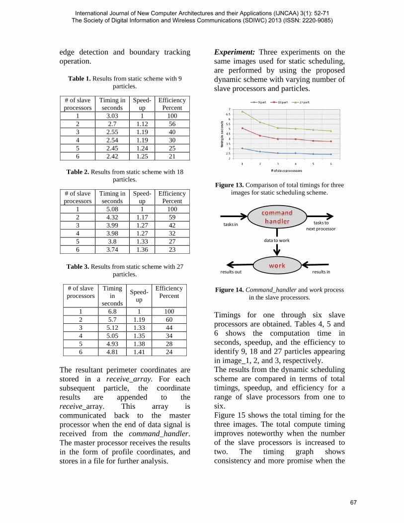
Experiment: Three experiments are performed on the proposed scheme with varying number of slave processors and particles. Figures 10, 11, and 12, show 9, 18, and 27 wear particle images appearing in image_1, image_2, and image_3, respectively. Timings for one through six slave processors are obtained. Tables 1, 2, and 3 shows the computation time in seconds, speedup, and the efficiency to identify wear

65


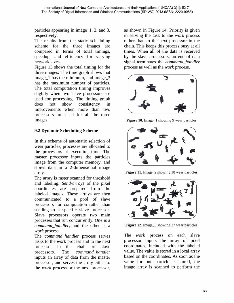
particles appearing in image_1, 2, and 3, respectively. The results from the static scheduling scheme for the three images are compared in terms of total timings, speedup, and efficiency for varying network sizes. Figure 13 shows the total timing for the three images. The time graph shows that image_1 has the minimum, and image_3 has the maximum number of particles. The total computation timing improves slightly when two slave processors are used for processing. The timing graph does not show consistency in improvements when more than two processors are used for all the three images. 9.2 Dynamic Scheduling Scheme In this scheme of automatic selection of wear particles, processes are allocated to the processors at execution time. The master processor inputs the particles image from the computer memory, and stores data in a 2-dimensional image array. The array is raster scanned for threshold and labeling. Send-arrays of the pixel coordinates are prepared from the labeled images. These arrays are then communicated to a pool of slave processors for computation rather than sending to a specific slave processor. Slave processors operate two main processes that run concurrently. One is a command_handler, and the other is a work process. The command_handler process serves tasks to the work process and to the next processor in the chain of slave processors. The command_handler inputs an array of data from the master processor, and serves the array either to the work process or the next processor,

as shown in Figure 14. Priority is given in serving the task to the work process rather than to the next processor in the chain. This keeps this process busy at all times. When all of the data is received by the slave processors, an end of data signal terminates the command_handler process as well as the work process.

Figure 10. Image_1 showing 9 wear particles.



The work process on each slave processor inputs the array of pixel coordinates, included with the labeled value. The value is stored in a local array based on the coordinates. As soon as the value for one particle is stored, the image array is scanned to perform the

66


edge detection and boundary tracking operation.

Table 1. Results from static scheme with 9 particles.

# of slave processors

Timing in seconds

Speed-up

Efficiency Percent

1 3.03 1 100 2 2.7 1.12 56 3 2.55 1.19 40 4 2.54 1.19 30 5 2.45 1.24 25 6 2.42 1.25 21

Table 2. Results from static scheme with 18

particles.


Timing in seconds

Speed-up

Efficiency Percent

1 5.08 1 100 2 4.32 1.17 59 3 3.99 1.27 42 4 3.98 1.27 32 5 3.8 1.33 27 6 3.74 1.36 23

Table 3. Results from static scheme with 27

particles.


Timing in

seconds

Speed-up

Efficiency Percent

1 6.8 1 100 2 5.7 1.19 60 3 5.12 1.33 44 4 5.05 1.35 34 5 4.93 1.38 28 6 4.81 1.41 24

The resultant perimeter coordinates are stored in a receive_array. For each subsequent particle, the coordinate results are appended to the receive_array. This array is communicated back to the master processor when the end of data signal is received from the command_handler. The master processor receives the results in the form of profile coordinates, and stores in a file for further analysis.

Experiment: Three experiments on the same images used for static scheduling, are performed by using the proposed dynamic scheme with varying number of slave processors and particles.

Figure 13. Comparison of total timings for three images for static scheduling scheme.

Figure 14. Command_handler and work process

in the slave processors. Timings for one through six slave processors are obtained. Tables 4, 5 and 6 shows the computation time in seconds, speedup, and the efficiency to identify 9, 18 and 27 particles appearing in image_1, 2, and 3, respectively. The results from the dynamic scheduling scheme are compared in terms of total timings, speedup, and efficiency for a range of slave processors from one to six. Figure 15 shows the total timing for the three images. The total compute timing improves noteworthy when the number of the slave processors is increased to two. The timing graph shows consistency and more promise when the

data to work

tasks tonext processor

tasks in

results inresults out

67


number of slave processors is increased from more than two.

Table 4. Results from dynamic scheme with 9

particles.


Timing in seconds

Speed-up

Efficiency Percent

1 3.4 1 100 2 2.35 1.43 71 3 2 1.68 56 4 1.93 1.74 44 5 1.87 1.79 36 6 1.87 1.79 30


particles.


Timing in seconds

Speed-up

Efficiency Percent

1 6.25 1 100 2 3.85 1.62 81 3 3.15 1.98 66 4 2.9 2.15 54 5 2.8 2.23 45 6 2.75 2.27 38


particles.


Timing in seconds

Speed-up

Efficiency Percent

1 8.9 1 100 2 5.15 1.66 83 3 3.99 2.23 74 4 3.55 2.51 63 5 3.44 2.59 52 6 3.35 2.66 44

Figure 15. Comparison of total timings for three

images for dynamic scheduling scheme.

10 COMPARISON The results from both the schemes of static and dynamic scheduling are compared for the three images, and over the range of network sizes. Figure 16 shows the timings for image_1, which has the minimum number of wear particles. The dynamic scheme takes more compute time than the static scheme when only one slave processor is used. Reasonable timings are achieved for the dynamic scheme by using two or more slave processors. However, the improvement is low but consistent. Figure 17 shows the compute timings for image_2, which has the moderate number of wear particles. The compute time improvement is consistent with the increased number of particles. Figure 18 shows the timings for image_3, which has the maximum number of wear particles. The dynamic scheme takes about nine seconds to compute 27 average sized particles, while the static scheme takes less than seven seconds when only one slave processor is used. The reason for this is that for static scheduling, the slave processor first inputs data for all the particles, and stores it in the local array. It then performs the edge detection on the overall image containing 27 particles when one slave is used. For dynamic scheduling, the processing for each particle is performed separately and it includes edge detection and boundary tracking. The timings improve for the dynamic scheme when two slave processors are used. Again, better results are achieved for dynamic scheduling when the number of slaves is increased. Figures 19 & 20, respectively, show the speedup, and efficiency graphs for both

68


schemes, and for all three images. The speedup improves slightly for the static scheme when the particle number and network size is increased. However, the speedup is significant for the dynamic scheme, especially for image_3.

Figure 16. Comparison of total timings for the two schemes for image_1.

Figure 17. Comparison of total timings for the

two schemes for image_2.

Figure 18. Comparison of total timings for the two schemes for image_3

The dynamic scheme out-performs the static scheme in terms of the speedup and efficiency for any number of wear particles. The reason being that in the static scheduling scheme, the master

processor distributes particle data to specific slave processors. As wear particles are typically of different sizes, it is more often that a specific slave processor receives particles that are larger in area than the others; therefore, this processor limits the performance of the system.

Figure 19. Comparison of speedup for the two

schemes Moreover, in the dynamic scheme, the command_handler in each slave makes sure that as soon as the work process completes the computation of the current job, another job is ready to be fed. By this means, the computation load is well balanced, and all of the slave processors complete their jobs concurrently. The results are also dependent on the number of particles that are required to be processed. With the increase in number of particles, the system performance improves for both the schemes.

Figure 20. Comparison of efficiency for the two

schemes.

69


11 CONCLUSION In this paper, methods used for parallelization of wear particle classification and recognition has been examined. By using the paradigms of problem decomposition, the performance of scheduling techniques is investigated for the parallel implementation of these types of algorithms on computer networks. Static and dynamic scheduling techniques have been investigated for the automatic wear particle selection over a range of network sizes and particle density. Performed experiments suggest that static scheme performs well with one slave processor. However, dynamic scheduling scheme outperforms its rival in terms of speedup and efficiency, and is well suited to the MIMD structure of computer networks. 12 REFERENCES 1. Hunter, R.C.: Engine Failure Prediction

Techniques. Aircraft Engineering 45, 4--13 (1975).

2. Pritchard, D.J.: Transputer Applications on Supernode. In: Proc. Int. Conf. on Application of Transputers, Liverpool, (1989).

3. Laghari, M.S., Khuwaja, G.A.: Processor Scheduling on Parallel Computers. In: Proc. Int. Conf. on Computer, Electrical, and Systems Sciences, and Engineering, Abu Dhabi (2012).

4. Laghari, M.S., Deravi, F.: Static vs. Dynamic Scheduling in Cellular Automaton. In Proc. Fall meeting # 4, North American Transputer User Group. New York (1990).

5. XU, K., Luxmoore, A.R., Jones, L.M., Deravi, F.: Integration of Neural Networks and Expert Systems for Microscopic Wear Particle Analysis. Knowledge Based Systems, vol. 11, no. 3, 213--222 (1998).

6. Laghari, M.S., Khuwaja, G.A.: Scheduling Techniques of Processor Scheduling in Cellular Automaton. In: Proc. Int. Conf. on Intelligent Computational Systems, pp. 96-100, Dubai (2012).

7. Peng, Z., Goodwin, S.: Wear Debris Analysis in Expert Systems. Tribology Letters, vol. 11, nos. 3-4, pp. 177-187, (2001).

8. Casavant, T.L., Kuhl, J.G.: A Taxonomy of Scheduling in General-Purpose Distributed Computing Systems. IEEE Trans. on Software Engineering, vol. 14, no. 2, (1988).

9. Raadnui, S.: Wear Particle Analysis—Utilization of Quantitative Computer Image Analysis: A Review. Tribology International, vol. 38, no. 10, pp. 871--878, (2005).

10. Laghari, M.S., Memon, Q.A., Khuwaja, G.A.: Knowledge Based Wear Particle Analysis. International Journal of Information Technology, vol. 1, no. 1, (2004).

11. Downton, A., Crookes, D.: Parallel Architectures for Image Processing. Electronics & Communication Engineering Journal 10, 139--151 (1998).

12. Talia, D., Srimani, P.K., Jazayeri, M.: Architecture-Independent Languages and Software Tools for Parallel Processing. IEEE Transactions on Software Engineering 26, 193--196 (2000).

13. Flynn, M.J.: Very High Speed Computing Systems. Proc. of the IEEE, vol. 54, no. 12, pp. 1901-1909, (1966).

14. Dongdong, M., Jinzong, L., Bing, Z., Fuzhen, Z.: Research on the Architectures of Parallel Image Processing Systems. In: Proc. 2nd Int. Symp. on Intelligent Information Technology Application, pp. 146--150, Shanghai (2008).

15. Zhang, N., Wang, J.: Image Parallel Processing based on GPU. In: Proc. 2nd Int. Conf. on Advanced Computer Control, pp. 367--370, Shenyang, (2010).

16. Krishnakumar, Y., Prasad, T.D., Kumar, K.V.S., Raju, P., Kiranmai, B.: Realization of a Parallel Operating SIMD-MIMD Architecture for Image Processing Application. In: Proc. Int. Conf. on Computer, Communication and Electrical Technology, Tamilnadu, India (2011).

17. Liu, H., Fan, Y., Deng, X., Ji, S.: Parallel Processing Architecture of Remotely Sensed Image Processing System Based on Cluster. In: Proc. 2nd Int. Congress on Image and Signal Processing, pp. 1--4, Tianjin (2009).

18. Wagner, A.S., Sreekantaswamy, H.V., Chanson, S.T.: Performance Models for the Processor Farm Paradigm. IEEE Trans. on

70


Parallel and Distributed Systems, vol. 8, no. 5, pp. 475-489, (1997).

19. Walsch, A.: Architecture and Prototype of a Real-Time Processor Farm Running at 1 MHz. Ph.D. Thesis, University of Mannheim, Germany (2002).

20. Jost, H.P.: Tribology – Origin and Future. Wear 136, 1--17 (1990).

21. Ruff, A.W.: Characterisation of Debris Particles Received from Wearing Systems. Wear 42, 49--62 (1977).

22. Bowen, E.R., Scott, D., Seifert, W., Westcott, V.C.: Ferrography. Tribology International 6, 109--115 (1976).

23. Cumming, A.C.: Condition Monitoring Today and Tomorrow – An Airline Perspective. In: Proc. 1st Int. Conf. on COMADEN’89, United Kingdom (1989).

24. Lukas, M., Anderson, D.P.: Analytical Tools to Detect and Quantify Large Wear Particles in Used Lubricant Oil. Technical report, Spectro Incorporated (2006).

25. Whitlock, R.R.: X-Ray Methods for Monitoring Machinery Condition. Advances in X-Ray Analysis 40, (1997).

26. Nunwong, P., Raadnui, S.: Wear Debris Assessment Utilizing Quantitative Image Analysis. In: Proc. 24th International Congress on Condition Monitoring and Diagnostics Engineering Management, Stavanger, Norway (2011).

27. Laghari, M.S.: Recognition of Texture Types of Wear Particles. Neural Computing & Applications 12, 18--25 (2003).

28. Khuwaja G.A., Laghari, M.S.: Computer Vision for Wear Debris Analysis. Int. Journal of Computer Applications in Technology, vol. 15, nos. 1/2/3, pp. 70--78, (2002).

29. Laghari M.S., Ahmed, F.: Computer Vision in the Field of Wear Particles. In: Proc. 2nd Int. Conf. on Computer and Electrical Engineering, Dubai (2009).

30. Laghari, M.S.: Shape and Edge Detail Analysis for Wear Debris Identification. IJCA 10, 271--279 (2003).

31. Albidewi, I.A.: The Application of Computer Vision to the Classification of Wear Particles in Oil. Ph.D. Thesis, University of Wales, Swansea (1993).

32. Anderson, D.P.: Wear Particle Atlas (revised). Naval Air Engineering Center, Lakehurst, New Jersey (1991).

33. Laghari, M.S.: Identification of Wear Particles in Oil by using Artificial Intelligence Techniques. In: Proc. 2nd International Conference on Modeling, Simulation, and Applied Optimization, Abu Dhabi (2007).

34. Yang, Y.S., Bahn, J.H., Lee, S.E., Bagherzadeh, N.: Parallel and Pipeline Processing for Block Cipher Algorithms on a Network-on-Chip. In: Proc. 6th Int. Conf. on Information Technology: New Generations, pp. 849--854, Las Vegas (2009).

35. Pavlidis, T.: Algorithms for Graphics and Image Processing. Computer Science Press, Rockville, MD (1982).

36. Kulpa, Z.: Area and Parameter Measurements of Blobs in Discrete Binary Pictures. Computer Graphics and Image Processing 6, 434--451 (1977).

37. Thomas, A.D.H.: The Application of Image Analysis to the Study of Wear Particles. Ph.D. Thesis, University of Wales, Swansea (1988).

38. Thomas, A.D.H., Davies, T., Luxmoore, A.R.: Computer Image Analysis for Identification of Wear Particles. Wear 142, 213--226 (1991).

39. Zingaretti, P., Gasparroni, M., Vecci, L.: Fast Chain Coding of Region Boundaries. IEEE Trans. Pattern Analysis and Machine Intelligence 20, 407—415 (1998).

71


Scheduling Techniques to Classify Wear Particles on...

Documents

Transcript of Scheduling Techniques to Classify Wear Particles on...