Theoretical Computer Science 369 (2006) 323–337www.elsevier.com/locate/tcs

Scheduling resource allocation with timeslot penalty forchangeover

Amrinder Arora∗, Fanchun Jin, Hyeong-Ah ChoiDepartment of Computer Science, The George Washington University, 801 22nd St. NW, Room 730, Washington, DC 20052, USA

Received 29 January 2006; accepted 14 September 2006

Communicated by A. Fiat

Abstract

Given a time slotted list of resource capacities, we address the problem of scheduling resource allocation considering that a changein allocation results in the changeover penalty of one timeslot. The goal is to maximize the overall allocation of resources. We provethat no 1-lookahead algorithm can be better than 8

5 -competitive. We provide improved analysis of Wait Dominate Hold (WDH)

algorithm that was previously known to be 4-competitive. We prove that WDH is 83 -competitive. We also consider k-lookahead

algorithms, and prove lower bound of (k + 2)/(k + 1) on their competitiveness and give an online algorithm that is 2-competitive.© 2006 Elsevier B.V. All rights reserved.

Keywords: Online scheduling; Changeover cost; Resource allocation; Wireless scheduling

1. Introduction

We consider an online scheduling problem with changeover costs defined as follows:Problem T RAC: Time slotted Resource Allocation with Changeover penalty:Given: Sequence of resource capacities C = [c(1), c(2), c(3), . . . , c(n)].To find: Allocation X = [x(1), x(2), x(3), . . . , x(n)], such thatx(i)�c(i) for 1� i�n (capacity constraint).If x(i) �= x(i + 2), then x(i + 1) = 0 (timeslot penalty for changeover).Objective function: To maximize

∑ni=1x(i).

An example problem instance of the T RAC problem and a feasible solution are shown in Table 1. We can easilyobserve that due to the timeslot penalty for changeover, a feasible solution to the problem must contain a 0 betweenunequal resource allocations.

∗ Corresponding author. Tel.: +1 202 994 4217; fax: +1 202 994 4875.E-mail addresses: amrinder@gwu.edu (A. Arora), jinfc@gwu.edu (F. Jin), hchoi@gwu.edu (H.-A. Choi).

0304-3975/$ - see front matter © 2006 Elsevier B.V. All rights reserved.doi:10.1016/j.tcs.2006.09.016

324 A. Arora et al. / Theoretical Computer Science 369 (2006) 323–337

Table 1A specific problem instance of T RAC and a feasible solution

C: 23 25 4 7 16 33 66 9 8 7 6 1X: 23 23 0 0 0 33 33 0 7 7 0 1

1.1. Motivation

The problem is directly motivated from the study of wireless networks. The capacities of the wireless channels canchange frequently, and the end points of the wireless channel can adjust the transmission parameters to adapt to thechannel condition. However, such an adjustment for transmission parameters needs the end points to communicateto adjust the data transfer configuration, which causes a loss of timeslots (the “changeover” cost). The end pointsmay decide to transmit data at lesser than available capacity, if by doing so, the changeover costs decrease. Theinteresting practical problem is to find a trade off between the benefit from the adjustment and the penalty caused byadjustment.

1.2. Background and previous work

Scheduling is one of the fundamental computer science problems. Basic setting of scheduling involves resources(machines) and jobs (tasks) that need to be scheduled, such that some metric (usually the makespan, that is the totallength of the schedule) is minimized. Many of the results in online scheduling can be attributed back to the 1966 paperby Graham [9], which was one of the first papers to consider the online scheduling problem, and to consider competitiveanalysis. The technique of competitive analysis, now commonly used in the context of online algorithms, comparesthe performance of online algorithm to that of an optimal offline algorithm. If the performance of an online algorithmA is at most c-times “worse” than the performance of an optimal offline algorithm, then the algorithm A is said to bec-competitive. In his landmark paper, Graham presented the list scheduling algorithm and proved that the competitiveratio of list scheduling algorithm is 2−1/m, where m is the number of machines. Graham’s work was finally improvedafter a hiatus of almost thirty years by Bartal et al. construction of an algorithm presented in [5]. Bartal et al.’s algorithmis 1.986 competitive, and was the first known algorithm with competitive ratio bounded less than 2 for all machines.That result was improved by Karger et al. [13], who presented an algorithm with competitive ratio of 1.945. In [2],Albers further improved the bound to 1.923-competitive by presenting an algorithm based on a different strategy, andalso improved the lower bound to 1.852.

Since Graham’s statement of scheduling problem, many different variations of online scheduling have also beenconsidered, such as preemptive scheduling, precedence constraints, release times, deadlines, conflicting jobs, unknownrunning times etc. A complete taxonomy of different variations of scheduling algorithms can be found in the textbook[6]. Optimal algorithm for online scheduling of parallel jobs with dependencies has been presented in [8]. Somesignificant papers in different variations of online scheduling include [19,10,17].

With respect to scheduling in wireless networks,Andrews and Zhang have presented excellent results on admissibilityof flows in [3]. Kalyanasundaram et al. have presented algorithm for minimizing average response time in [12]. Othersignificant papers for the applications of scheduling problem in wireless networks include [14–16] etc.

1.3. Our results

We focus entirely on the technique of competitive analysis. Our current work is an extension of results earlierpresented in [4,18,11]. In those papers, it was shown that no online algorithm with finite lookahead can be optimal.A dynamic programming algorithm for the offline solution was given, that executes in O(n3) time, where n is thenumber of timeslots. A 1-lookahead online algorithm (wait dominate hold (WDH) algorithm) was also presented, andit was shown to be 4-competitive.

In this paper, we improve the results significantly, and also consider new problem variations. After observing that analgorithm with no lookahead cannot be c-competitive for any c, we focus on 1-lookahead algorithms. We prove that no1-lookahead algorithm can be better than 8

5 -competitive. The proof uses an adaptive offline adversary, and the central

A. Arora et al. / Theoretical Computer Science 369 (2006) 323–337 325

Table 2Summary of results presented in this paper

Lookahead 1 2 k > 2Lower bound 8/5 4/3 (k + 2)/(k + 1)

Upper bound 8/3 2 2

idea is that adversary increases the capacity if the online algorithm does not use a timeslot, and keeps it constant ifthe adversary uses a timeslot. Without considering the boundary condition, it can be easily shown that the adversarycan always achieve twice the total allocation as the online algorithm. Since the resource capacity keeps increasing inthe adversary’s constructed example, we focus on the boundary condition closely, and prove that even including theboundary condition, no 1-lookahead algorithm can be better than 8

5 -competitive.We provide improved analysis of WDH algorithm. We prove that WDH is 8

3 -competitive. We use a novel techniqueof tracking internal states of the algorithm in terms of a finite state automata, and analyze all different sentences that canbe possibly generated by the WDH algorithm. We hope that the same technique can be used to analyze other algorithmsas well.

We also consider k-lookahead algorithms for the resource allocation problem, and prove lower bound of (k+2)/(k+1)

using the adversary approach. As expected, this lower bound approaches 1 as k increases.We give a simple online algorithm that is 2-competitive when there is at least 2 lookahead available. Before giving

that algorithm, we present two general families of online k-lookahead algorithms—the Optimal Block Algorithm(OPTB) and Optimal Sliding Window Algorithm (OPTSW). We believe that OPTB and OPTSW can be considered asgeneral frameworks for many online problems that use the concept of “timeslot” or “step” and where the lookahead isavailable.

A summary of our results is presented in Table 2.

1.4. Structure of the paper

This paper is organized as follows. This section covers the problem statement, motivation and the previous workdone in the related fields. Section 2 presents the lower bound for all one lookahead algorithms for T RAC problem. Inthe Section 3, we present an improved analysis of the WDH algorithm and prove that it is 8

3 -competitive, improvingthe earlier known analysis of 4-competitive. We consider the k-lookahead variation of the problem in Section 4 andpresent lower and upper bounds. Our conclusions in Section 5 complete the paper.

2. Lower bound analysis for 1-lookahead algorithms

Firstly, we note that for online scheduling problem with one timeslot penalty as changeover cost, an algorithm with0-lookahead cannot be c-competitive for any value of c. As an example, suppose that capacity of the first timeslot is 1.If an online algorithm with no lookahead does not use resource at all in this timeslot, then the adversary can simplyterminate and use the resource fully. If the online algorithm uses the resource (either partially, or fully) in this timeslot,then the adversary can use a high value of resource capacity in the second timeslot, which the algorithm will be unableto use. In either case, the competitive ratio is not bounded by any constant.

In this section, we prove a lower bound on all 1-lookahead algorithms. Consider a deterministic 1-lookahead onlinealgorithm A . For the purpose of this discussion, let a(t) denote the output selected by algorithm A during timeslot t ,let x(t) denote the output selected by the constructed offline solution, and let |A| denote the total allocation achievedby A .

Consider input of 1, 2, c(3), where value of c(3) is controlled by an adaptive online adversary.If algorithm A chooses a(1) > 0 in the first slot, adversary sets the value of c(3) = a(1) − �. In this case, the

algorithm can only achieve a total allocation of 2a(1), while optimal total allocation is 3a(1)−3�. If algorithm choosesa(1) = 0 in the first slot, adversary sets the value of c(3) = 1. In this case, the algorithm can only achieve a totalallocation of 2, while optimal total allocation is 3. Thus, no 1-lookahead online algorithm can achieve a total allocationof more than 2

3 times that of optimal.

326 A. Arora et al. / Theoretical Computer Science 369 (2006) 323–337

This counterexample proves a lower bound of 32 on competitive ratio of 1-lookahead algorithms. Next, we formulate

the following adversary strategy to prove a better lower bound:Adversary strategy: Start with an input of c(1) = 1 and c(2) = 2. Set the value of c(t), for all t > 2 based on choice

of online algorithm as per following rules:Adversary rule 1: If a(t − 2) = 0, set c(t) = 2c(t − 1).Adversary rule 2: If a(t − 2) > 0, set c(t) = c(t − 1).Based on online algorithm A , a sample input and algorithm can be like:c(t): 1 2 . . . 2k1 2k1+1 . . . 2k1+1 2k1+1 2k1+1 2k1+2,

a(t): 0 0 . . . a1 . . . . . . a1 0.Constructing an offline solution: Consider an offline solution, that uses the full capacity on any timeslot that succeeds

a timeslot where algorithm’s choice is not 0. That is, if a(t) > 0, then set x(t + 1) = c(t + 1).

Lemma 1. Offline solution as defined above is a valid solution.

Proof. To see that the offline solution as defined above is a valid solution, we only need to prove that if for any twoconsecutive timeslots, offline solution allocates non-zero outputs, then both the values are the same. Suppose, duringtimeslots t + 1 and t + 2, the offline allocation is non-zero. Therefore, by definition, a(t) > 0 and a(t + 1) > 0.Since a(t) > 0, by definition of capacity matrix, c(t + 2) = c(t + 1). Thus, by construction of offline solution,x(t + 2) = c(t + 2) = c(t + 1) = x(t + 1). Therefore, the offline solution as constructed above is a valid solution. �

Theorem 1. Excluding boundary condition, offline solution as constructed above achieves a total value of twice thatof the one step lookahead online algorithm A .

Proof. We prove this claim by demonstrating a bijection between the allocations made by A and the constructed offlinesolution. Specifically, we prove using induction that for each timeslot t , for which a(t) > 0, x(t + 1)�2a(t).

Induction base: Clearly, this claim is true for t = 1, as c(1) = 1 and c(2) = 2. If a(1) > 0, then x(2) = 2�2a(1).Induction hypothesis: Let us assume that the claim is true for all t < T .Induction step: Suppose a(T ) > 0, then by definition, x(T + 1) = c(T + 1), and there are two cases:

If a(T − 1) = 0, then c(T + 1) = 2c(T ), and thus x(T + 1)�2a(T ).If a(T − 1) > 0, then a(T ) = a(T − 1) and c(T + 1) = c(T ), and thus x(T + 1) = x(T ). Using induction hypothesis,x(T )�2a(T − 1). Thus, x(T + 1)�2a(T ).

Thus, having proved a bijection, we know that excluding boundary conditions,∑

t x(t)�2∑

t a(t). �

2.1. Fixing boundary condition

The discussion in the preceding sections presents an intuitive idea for adversary. However, it does not suggest asuitable end point for the algorithm. For example, if the online algorithm continues to allocate a(t) = 0, the adversarycontinues to set c(t + 1) = 2c(t) ad infinitum. In this section, we present a method to find a suitable end point. Weintend to prove that no online algorithm can be better than c-competitive, where c = 8/5 − �.

To prove that, we first generalize the previous strategy, by replacing the constant 2 with a constant �, where � ∈( 5

3 , 2]. Next, we make two observations. Both of these observations are in the context of the adversary strategy presentedabove.

Lemma 2. If the online algorithm A uses a contiguous block of �5/(3� − 5)� elements, then the adversary can achievea ratio of 5

3 .

Proof. Consider an input sequence as follows:c(t): 1 � . . . � � 0,a(t): 1 1 . . . 1.If algorithm uses a contiguous block of k elements, the adversary can stop by putting a 0 in the last timeslot. In this

case, A achieves total allocation of k + 1, and adversary achieves total allocation of �k, that is, a ratio of �k/(k + 1),which is more than 5

3 if k�5/(3� − 5). �

A. Arora et al. / Theoretical Computer Science 369 (2006) 323–337 327

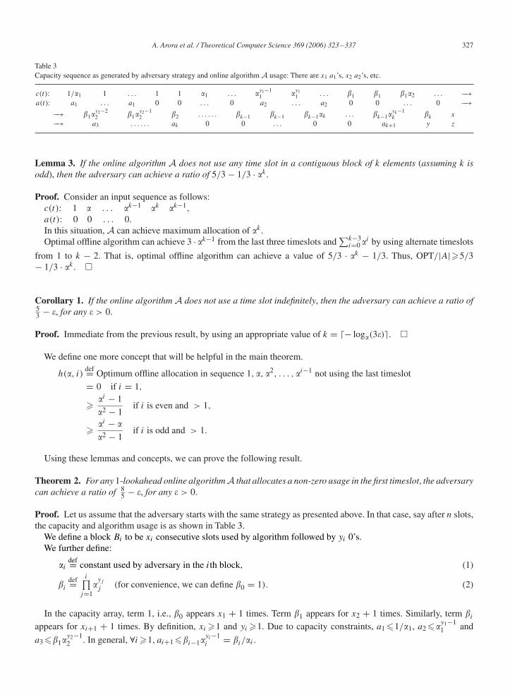
Table 3Capacity sequence as generated by adversary strategy and online algorithm A usage: There are x1 a1’s, x2 a2’s, etc.

c(t): 1/�1 1 . . . 1 1 �1 . . . �y1−11 �y1

1 . . . �1 �1 �1�2 . . . −→a(t): a1 . . . a1 0 0 . . . 0 a2 . . . a2 0 0 . . . 0 −→

−→ �1�y2−22 �1�

y2−12 �2 . . . . . . �k−1 �k−1 �k−1�k . . . �k−1�

yk−1k �k x

−→ a3 . . . . . . ak 0 0 . . . 0 0 ak+1 y z

Lemma 3. If the online algorithm A does not use any time slot in a contiguous block of k elements (assuming k isodd), then the adversary can achieve a ratio of 5/3 − 1/3 · �k .

Proof. Consider an input sequence as follows:c(t): 1 � . . . �k−1 �k �k−1,

a(t): 0 0 . . . 0.In this situation, A can achieve maximum allocation of �k .Optimal offline algorithm can achieve 3 · �k−1 from the last three timeslots and

∑k−3i=0 �i by using alternate timeslots

from 1 to k − 2. That is, optimal offline algorithm can achieve a value of 5/3 · �k − 1/3. Thus, OPT/|A|�5/3− 1/3 · �k . �

Corollary 1. If the online algorithm A does not use a time slot indefinitely, then the adversary can achieve a ratio of53 − �, for any � > 0.

Proof. Immediate from the previous result, by using an appropriate value of k = �− log�(3�)�. �

We define one more concept that will be helpful in the main theorem.

h(�, i)def= Optimum offline allocation in sequence 1, �, �2, . . . , �i−1 not using the last timeslot

= 0 if i = 1,

� �i − 1

�2 − 1if i is even and > 1,

� �i − �

�2 − 1if i is odd and > 1.

Using these lemmas and concepts, we can prove the following result.

Theorem 2. For any 1-lookahead online algorithm A that allocates a non-zero usage in the first timeslot, the adversarycan achieve a ratio of 8

5 − �, for any � > 0.

Proof. Let us assume that the adversary starts with the same strategy as presented above. In that case, say after n slots,the capacity and algorithm usage is as shown in Table 3.

We define a block Bi to be xi consecutive slots used by algorithm followed by yi 0’s.We further define:

�idef= constant used by adversary in the ith block, (1)

�idef=

i∏

j=1�yj

j (for convenience, we can define �0 = 1). (2)

In the capacity array, term 1, i.e., �0 appears x1 + 1 times. Term �1 appears for x2 + 1 times. Similarly, term �i

appears for xi+1 + 1 times. By definition, xi �1 and yi �1. Due to capacity constraints, a1 �1/�1, a2 ��y1−11 and

a3 ��1�y2−12 . In general, ∀i�1, ai+1 ��i−1�

yi−1i = �i/�i .

328 A. Arora et al. / Theoretical Computer Science 369 (2006) 323–337

Each 0 in the algorithm allocation array makes the entry in the capacity array increase by a factor of �i , for some i.The algorithm A and optimal achieve a total of

|A| =k∑

i=1aixi + opt[ak+1, y, z], (3)

OPT =k∑

i=1{�i−1xi + �i−1h(�i , yi)} + opt[�k/�k, �k, x]

�k∑

i=1{�i−1aixi + �i−1h(�i , yi)} + opt[�k/�k, �k, x]. (4)

Using results presented above, we observe that if for any i, xi ��5/(3�i − 5)�, then the adversary could terminateat that point. Also, if yi ��− log�(3�)�, the adversary could terminate. Thus, we assume that for all i ∈ {1 . . . k},xi < �5/(3�i − 5)� and yi < �− log�(3�)�. This also allows us to assume that the adversary can force the algorithmto have as many blocks as it wants, since each block size is bounded.

Consider adversary’s choice of �i = 2 for i ∈ {1, . . . , k − 1} and �k = 53 + �1.

Suppose S = ∑ki=1aixi . Then, we have that

|A| = S + 2ak+1,

OPT � 2S + �k−1h(�k, yk) + 3(ak+1 − �2),

OPT � 2S + �k−1(�yk

k − �k)/(�2k − 1) + 3(ak+1 − �2).

Now consider ak+1, it is the value chosen by the algorithm in the (k + 1)th block. It is clear from the equation, thatthe best competitive ratio is obtained by the algorithm when ak+1 is as large as possible. Thus, say ak+1 = �k−1�

yk−1k .

We thus obtain that|A| = S + 2�k−1�

yk−1k .

OPT�2S + �k−1(�yk

k − �k)/(�2k − 1) + 3�k−1�

yk−1k − 3�2.

Three cases arise on value of yk:Case I: yk = 1.|A| = S + 2�k−1.OPT�2S + 3�k−1 − 3�2.⇒ OPT�8/5|A| + 0.2(2S − �k−1) − 3�2.Knowing that 2S��k−1, we obtain that OPT�8/5|A| − �, where � = 3�2.Case II: yk = 2.|A| = S + 10/3�k−1.OPT�2S + 6�k−1 − 3�2.OPT�9/5|A| − 3�2.Case III: yk > 2.|A| = S + 2�k−1�

yk−1k .

OPT�2S + �k−1�yk

k − �9/25 − �4 + 3�k−1�yk−1k − 3�2.

OPT�2S + 18/5�k−1�yk−1k − 3/5�k−1 − 3�2.

OPT�9/5|A| − 3�2.Taking the minimum value of competitive ratio from the three cases, we obtain that

OPT�8/5|A| − �. �

Theorem 2 can be easily extended to all online algorithms by combining results of the Lemma 3.

Theorem 3. For any online algorithm A , the adversary can achieve a ratio of 85 − �, for any � > 0.

A. Arora et al. / Theoretical Computer Science 369 (2006) 323–337 329

Proof. If A does not use any of the first �− log�(3�)� time slots, then by Lemma 3, the adversary can achieve a ratioof 5

3 − � and stop. If the algorithm does use a timeslot, then the adversary can simply ignore all prior timeslots, andthen using Theorem 2, the adversary can achieve a ratio of 8

5 − �, for any � > 0. �

3. WDH algorithm

In this section, we analyze the WDH online algorithm as presented in [4].We use the following two definitions as part of our analysis.Strongly increasing sequence: A sequence of numbers is said to be strongly increasing if each number is at least

twice as much as the previous number.Almost equal: Two numbers are said to be almost equal if neither is more than or equal to twice the other.

We represent it as x ≈ y.

3.1. Background and definition of WDH

The WDH algorithm is a one step lookahead online algorithm. Before allocating usage for a time slot, it uses thefollowing information: allocation in the previous timeslot x(t − 1), current capacity c(t) and next capacity c(t + 1).

WDH algorithm uses the following set of rules for choosing x(t):(Pre-calculation) If x(t − 1) = 0, set u(t) = c(t), else u(t) = min{x(t − 1), c(t)}.(R1) If c(t + 1) > 2u(t), set x(t) = 0.(R2) If u(t)�2c(t + 1), set x(t) = u(t) (note that x(t + 1) will be assigned to 0 in the next slot schedule).(R3) If c(t + 1)/2�u(t) < 2c(t + 1) and x(t − 1) > 0, set x(t) = u(t).(R4) If c(t + 1)/2�u(t) < 2c(t + 1) and x(t − 1) = 0, set x(t) = min{u(t), c(t + 1)}.

Note that (R1) corresponds to Wait, (R2) corresponds to Dominate, and (R3) and (R4) correspond to Hold.The precise definition of the algorithm is presented in Table 4.An example usage of the WDH algorithm is shown in Table 5.

3.2. Competitive analysis of WDH algorithm

In [4], it was proven that WDH algorithm is 4-competitive. The analysis was against the total capacity, not againstthe optimal offline solution.

We present an improved analysis. This novel analysis technique tracks the internal states of the WDH algorithm.

Table 4Wait-dominate-hold: A 1-slot lookahead online algorithm

double waitDominateHold (double prevUsage, double currCapacity, double nextCapacity){// Calculates the upper bound for usage in this cycledouble ub = 0;if (prevUsage > currCapacity)return 0;

else if (prevUsage?= 0)

ub = currCapacity;elseub = prevUsage;

// Waits (next capacity is very high)if (2 * ub < nextCapacity)return 0;

// Dominates (next capacity is very low)if (ub � 2 * nextCapacity)return ub;

// If previous slot was used, it is not allowed to Hold.if (prevUsage > 0)return ub;

// Hold and waitreturn min (ub, nextCapacity);}

330 A. Arora et al. / Theoretical Computer Science 369 (2006) 323–337

Table 5Example usage of wait-dominate-hold algorithm

C: 23 25 4 7 16 33 66 9 8 7 6 1X: 23 23 0 0 0 33 33 0 7 7 0 1

q1 q2

q4

q0 q3H C S

DD S

W H

ε

ε

Fig. 1. Automata.

3.2.1. Definition of return statesBy analyzing Table 4, we can associate each “return” statement with a corresponding return state. Following states

can be identified:• S: Suffer: Allocation of previous timeslot was more than capacity of current timeslot.• W : Wait: Capacity of next timeslot is more than twice the maximum possible usage in current timeslot.• D: Dominate: Capacity of next timeslot is less than half the maximum possible usage in current timeslot.• H : Hold: Capacity of next timeslot is approximately (within a factor of two) of current maximum possible usage.• C: Continue: Would like to dominate/hold, but have to maintain allocation of previous timeslot.

3.2.2. Rules governing the internal states of WDH algorithmRules:

• C can only be followed by S.• D can only be followed by S.• H can be followed by W, D, H or C, but not by S.• W can be followed by W, D or H , but not by C or S.• S can be followed by W, D or H , but not by C or S.The automata representing the state transitions of WDH algorithm is shown in Fig. 1.

3.2.3. Defining the sentencesFrom the automata shown in Fig. 1, it is clear that the sentences that can be generated using WDH are as follows:

1. W ∗DS;2. W ∗H+CS;3. W ∗H+DS;4. W ∗H+.Thus, possible sentences are: {W ∗DS|W ∗H+CS|W ∗H+DS|W ∗H+}∗.

We observe an interesting element from these sentences that when H is followed by W , it could be either becausethe capacity for that timeslot was lesser than half of the next capacity, or because the possible allocation was lesser

A. Arora et al. / Theoretical Computer Science 369 (2006) 323–337 331

than half of the next capacity. We further observe that any sentence that follows W ∗H+ sentence must have at leastone W . To account for that, we consider the possible sentence W ∗H+ to include a W at the end, that is, W ∗H+W . Aswe will observe in Section 3.2.8, we analyze this sentence in two separate cases and can then decide if the last W inthat sentence should be analyzed as part of that sentence of a different sentence.

3.2.4. Useful lemmaWe use the following lemma in some of the proofs. This lemma is similar to the definition of h(�, i) given in Section

2 in the lower bound analysis, using a constant value of 2 for �.

Lemma 4. Given a strongly increasing sequence of capacities, the maximum allocation that can be achieved is nomore than 4

3 times the capacity of the last timeslot.

Proof.Given: C : c(1), c(2), . . . , c(k), such that2c(i)�c(i + 1) ∀i ∈ 1 . . . k − 1.To prove: Optimal allocation, opt(C)�4/3c(k).Case I: k is even.

opt(c(1), c(2), . . . , c(k)) � opt(c(1), c(2)) + · · · + opt(c(k), c(k − 1))

� c(2) + · · · + c(k)

� 4/3c(k).

Case II: k is odd.

opt(c(1), c(2), . . . , c(k)) � c(1) + opt(c(2), c(3)) + · · · + opt(c(k, c(k − 1)))

� c(1) + c(3) + · · · + c(k)

� 4/3c(k). �

Next, we analyze the four different sentences independently.

3.2.5. Analysis of W ∗DS sentenceInput

C : c(1), . . . , c(k), c(k + 1), c(k + 2).2c(i)�c(i + 1) ∀i ∈ {1 . . . k}.2c(k + 2)�c(k + 1).

WDH outputX : 0, 0, . . . , 0, c(k + 1), 0.

Optimal solutionc(1), 0, c(3), 0, c(5), . . . , 0, c(k + 1), 0 (If k is even).0, c(2), 0, c(4), 0, c(6), . . . , 0, c(k + 1), 0 (If k is odd).

|OPT | = c(k + 1) + c(k − 1) + c(k − 3) + · · ·� c(k + 1) + 1/4c(k + 1) + 1/16c(k + 1) + · · ·� 4/3c(k + 1).

ResultCompetitive ratio: 4/3.

332 A. Arora et al. / Theoretical Computer Science 369 (2006) 323–337

3.2.6. Analysis of W ∗H+CS sentenceInput

C : c(1), . . . , c(k), c(k + 1), c(k + 2), . . . , c(k + n + 1), c(k + n + 2).2c(i)�c(i + 1) ∀i ∈ {1 . . . k}.c(k + i) ≈ c(k + j) ∀i, j ∈ {1 . . . n + 1}.c(k + i) > c(k + n + 2) ∀i ∈ {1 . . . n + 1}.

WDH output

X : 0, 0, . . . , 0, y, y, . . . , y︸ ︷︷ ︸n+1

, 0.

Note that y = min{c(k + 1), c(k + 2), . . . , c(k + n + 1)}.Optimal solution

Suppose that z = max{c(k + 1), c(k + 2), . . . , c(k + n + 1)}.Note that y > c(k + n + 2).

|OPT | � 4/3c(k) + max{nz, (n + 1)y} + c(k + n + 2)

� 4/3y + max{nz, (n + 1)y} + y

� (2n + 1 + 4/3)y.

|OPT |/|X|�(2n + 1 + 4/3)/(n + 1)�13/6.

ResultCompetitive ratio: 13/6.

3.2.7. Analysis of W ∗H+DS sentenceInput

C : c(1), . . . , c(k), c(k + 1), c(k + 2), . . . , c(k + n + 1), c(k + n + 2).2c(i)�c(i + 1) ∀i ∈ {1 . . . k}.c(k + i) ≈ c(k + j) ∀i ∈ {1 . . . n + 1}.c(k + i) > 2c(k + n + 2) ∀i ∈ {1 . . . n + 1}.

WDH output

X : 0, 0, . . . , 0, y, y, . . . , y︸ ︷︷ ︸n+1

, 0.

Note that y = min{c(k + 1), c(k + 2), . . . , c(k + n + 1)}.Optimal solution

Suppose that z = max{c(k + 1), c(k + 2), . . . , c(k + n + 1)}.Note that y > 2c(k + n + 2).

|OPT | � 4/3c(k) + max{nz, (n + 1)y} + c(k + n + 2)

� 4/3y + max{nz, (n + 1)y} + 1/2y

� (2n + 1/2 + 4/3)y.

|OPT |/|X|�(2n + 1/2 + 4/3)/(n + 1)�23/12.

ResultCompetitive ratio: 23/12.

A. Arora et al. / Theoretical Computer Science 369 (2006) 323–337 333

3.2.8. Analysis of W ∗H+W sentenceInput

C : c(1), . . . , c(k), c(k + 1), c(k + 2), . . . , c(k + n), c(k + n + 1).

2c(i)�c(i + 1) ∀i ∈ {1 . . . k}.c(k + i) ≈ c(k + j) ∀i, j ∈ {1 . . . n}.2c(k + i)�c(k + n + 1) ∀i ∈ {1 . . . n}.

WDH output

X : 0, 0, . . . , 0, y, y, . . . , y︸ ︷︷ ︸n

, 0.

Note that y = min{c(k + 1), c(k + 2), . . . , c(k + n)}.Optimal solution

Suppose that z = max{c(k + 1), c(k + 2), . . . , c(k + n)}.Note that 2y�c(k + n + 1).

Case 1: n = 1We consider two cases on the values of c(k + 1) and c(k + 2).

• y = c(k + 1) < c(k + 2).Note that y > 2c(k).

|OPT | � 4/3c(k) + 2y

� 2/3y + 2y

� 8/3y.

• y = c(k + 2)�c(k + 1).In this case, note that WDH output is X : 0, 0, . . . , 0, y, 0 where y = c(k + 2), such that xk+2 = 0 because of2c(k + 2) < c(k + 3), where c(k + 3) is located in the next sentence. If we take off c(k + 2) from and the currentsentence, and append it in front of the next sentence, it will not affect the analysis of the next sentence, since newlygenerated W ∗ in the next sentence is still strongly increasing. Now we analyze the current sentence without c(k +2).

|OPT | � 4/3c(k) + y

� 4/3y + y

� 7/3y.

Case 2: n > 1

|OPT | � 4/3c(k) + max{nz, (n + 1)y}� 4/3y + max{nz, (n + 1)y}� (2n + 4/3)y.

|OPT |/|X|�(2n + 4/3)/n�8/3 when n > 1.Result

Competitive ratio: 8/3.

3.2.9. Putting it all togetherTheorem 4. WDH algorithm is 8

3 -competitive.

Proof. Immediate from results of preceding sections, as we take the maximum value of competitive ratios of all foursentences. �

334 A. Arora et al. / Theoretical Computer Science 369 (2006) 323–337

3.3. Tightness of competitive analysis of WDH algorithm

Next, we present an example where optimal allocation is twice the allocation of WDH algorithm.

C 1 2 2 2 . . . 2WDH 1 1 1 1 . . . 1OPT 0 2 2 2 . . . 2

In this case, the optimal allocation approaches twice the allocation of WDH algorithm, and can be made arbitrarilyclose to 2 by changing the length of the input.

4. Problem variation: k-lookahead algorithms

Having proved both upper and lower bounds for the 1-lookahead online problem, we now focus on the k-lookaheadvariation. As outlined in [1], considering k-lookahead is a natural extension of online problems, both in the theoretical,and in the practical sense (the authors in that paper pose quite eloquently “What is it worth to know a part of the future”).Online scheduling problem with k-lookahead was also considered in [7] in the context of web caching. In [1], twomodels of lookahead for online algorithms were presented, weak k-lookahead (in which next k requests are known)and strong k-lookahead (in which k distinct requests are known). In this paper, we focus on the weak k-lookahead, asdistinctness of capacity values does not fundamentally change our problem definition.

We consider online algorithms that have k-timeslots lookahead information available, where k > 1. In such a case,the problem can be stated as:

Given: x(t − 1), c(t), c(t + 1), . . . , c(t + k).To find: x(t).We refer to x(t − 1) as the previous allocation, c(t) as the current capacity and c(t + 1) . . . c(t + k) as the lookahead

capacities. We observe that if k = 0, then no competitive ratio is possible, and that if k = 1, then the results presentedin Sections 2 and 3 are the best known results.

4.1. A lower bound on all k-lookahead algorithms

Theorem 5. No k-lookahead online algorithm can be better than ((k + 2)/(k + 1))-competitive.

Proof. Let us assume that there are a total of k + 2 timeslots, and the adversary sets c(i) = 1 ∀i ∈ {1 . . . k + 1}.Suppose the online algorithm A allocates value of a in the first timeslot. Let us denote the maximum allocation achievedby A by |A|. We consider two cases on the value of a:

Case I: a�k/(k + 1). In this case, adversary can set c(k + 2) = a − �.In this case algorithm A must miss at least one timeslot, as its current allocation exceeds the capacity available in

the last timeslot.|A|�a(k + 1), while |OPT | = (k + 2)(a − �)Thus |OPT |/|A|�(k + 2)/(k + 1).Case II: a < k/(k + 1). In this case, adversary can set c(k + 2) = 1.Algorithm A can continue to use a for all timeslots in which case it achieves a total allocation of a(k + 2) or it can

miss one timeslot and allocate value of 1 for all other timeslots. In either case, |A|�k + 1, while |OPT | = k + 2Thus |OPT |/|A|�(k + 2)/(k + 1). �

4.2. Two families of k-lookahead online algorithms

In this section, we present two families of k-lookahead algorithms for all online problems for which an optimaloffline algorithm is known.

A. Arora et al. / Theoretical Computer Science 369 (2006) 323–337 335

Table 6OPTB Algorithm: t = 0 is the current decision task

past state︷ ︸︸ ︷. . . − 2 − 1 0

lookahead︷ ︸︸ ︷

1 2 3︸ ︷︷ ︸boundary

4 5 . . . . . . k − 3︸ ︷︷ ︸inner timeslots

k − 2 k − 1 k

Definitions of inner and boundary timeslots vary by exact problem instance.

4.2.1. OPTB: Optimal Block AlgorithmGiven the current state of the algorithm, and the k-lookahead information, the OPTB algorithm proceeds as follows.

1. Divide the input into blocks of size k each (or nearly k, depending upon exact problem).2. Use the known optimal offline algorithm to find the optimal solution for each block.3. Use the solution to set values of all “inner” timeslots. Set values of “boundary” timeslots as per the boundary

constraints of the problem and local optimization.We observe that the exact block size, the definition of inner and boundary timeslots is defined by the exact problem.

A conceptual drawing of OPTB is shown in Table 6.Time complexity of OPTB: Assuming the time complexity of the optimal offline algorithm is f (k), and the time for

local optimization is constant, the average time complexity of the OPTB algorithm is O(f (k)/k) per timeslot. We notethat the maximum time spent is O(f (k)), which is applicable every kth timeslot. That may be the correct metric toapply in certain situations, for example, embedded systems that have limited hardware.

4.2.2. OPTSW: Optimal Sliding Window AlgorithmGiven the current state of the algorithm, and the k-lookahead information, the OPTSW algorithm proceeds as follows:

1. Use the known optimal offline algorithm to find the optimal schedule for each block.2. Take the decision for the current timeslot (or job) only based on the boundary constraints and the solution of the

optimal offline algorithm.3. At each timeslot execute the algorithm again.

Time Complexity of OPTSW: Assuming that the time complexity of the optimal offline algorithm is f (k), and thetime for resolving boundary constraints is constant, we can infer that the time complexity of the OPTSW algorithm isO(f (k)) per timeslot.

4.2.3. Applying Optimal Block Algorithm to our problemNext, we consider the natural application of OPTB to our problem, where we use the dynamic programming offline

optimal algorithm given in [4].1. As per OPTB, we divide the input into m blocks of size k each. Say the block Bi consists of timeslots ik + 1, ik +

2, . . . , ik + k. Blocks are numbered as B0, B1, . . . , Bm−1.2. We use the known optimal offline algorithm to find the optimal schedule for the block Bi .3. Set allocation for timeslots ik + 1, ik + 2, . . . ik + k − 1 as per the optimal schedule.4. Before setting the allocation for ik + k, calculate optimal schedule for block Bi+1. We observe that as the algorithm

is k-lookahead, the resource capacities for block Bi+1 are available before a decision needs to be made for ik + k

timeslot.5. For timeslots ik + k and ik + k + 1, if the values x(ik + k) and x(ik + k + 1) are equal, set both of them, otherwise

set the smaller of them to 0.

Theorem 6. Algorithm OPTB is 2-competitive, for all k�2.

Proof. Clearly, the sum of optimal offline solutions constructed for each block is at least as large as the optimal offline.

∑

i

Bi �OPT .

336 A. Arora et al. / Theoretical Computer Science 369 (2006) 323–337

We observe that actual allocation made is different from the sum, as the smaller of the two elements: x(ik + k) andx(ik + k + 1) is set to 0, unless the two elements are equal.

⇒ ∑

i

B ′i �

∑

i

Bi − ∑

i

min{xik, xik+1}. (5)

The sum of solutions for each block contains both these elements, among others.

⇒ ∑

i

Bi �∑

i

{xik + xik+1}. (6)

From Eqs. (5) and (6), we can deduce that

⇒ ∑

i

B ′i � Bi/2,

⇒ ∑

i

B ′i � OPT/2. �

Note on time complexity: Since the time complexity of the dynamic programming algorithm is O(k3), the timecomplexity of the OPTB algorithm is O(k2) per timeslot. As k increases, this may increase while providing verylittle additional increase in performance. In that case, a constant value of k (such as 10) should be adopted as per thesimulation results and practical requirements.

5. Conclusions

We consider a fundamental resource allocation problem that has a constraint that a change in allocation results inthe changeover penalty of one timeslot. The problem is directly motivated from scheduling of capacity in wirelessnetworks.

After observing that an algorithm with no lookahead cannot be c-competitive for any c, we focussed on 1-lookaheadalgorithms. We proved that no 1-lookahead algorithm can be better than 8

5 -competitive. The proof uses an adaptiveoffline adversary, and the central idea is that adversary increases the capacity if the online algorithm does not use atimeslot, and keeps it constant if the adversary uses a timeslot. We proved that no 1-lookahead algorithm can be betterthan 8

5 -competitive.We have presented improved analysis of Wait Dominate Hold (WDH) algorithm that was previously known to be

4-competitive. We proved that WDH is 83 -competitive. We use a novel technique of tracking internal states of the

algorithm in terms of a finite state automata, and analyzed the different sentences that can be possibly generated by thereturn states of the WDH algorithm. We hope that the same technique can also be used to analyze other algorithms.

We have also considered k-lookahead algorithms for the resource allocation problem, and have proven lower boundof (k + 2)/(k + 1) using the adversary approach. As expected, this lower bound approaches 1 as k increases.

We have presented a simple online algorithm that is 2-competitive when there is at least 2 lookahead available.Before giving that algorithm, we present two general families of online k-lookahead algorithms—the Optimal BlockAlgorithm (OPTB) and Optimal Sliding Window Algorithm (OPTSW). We believe that OPTB and OPTSW can beconsidered as general frameworks for many online problems that use the concept of “timeslot” or “step” and wherelookahead is available.

Future work in this field can focus on (i) further improving the analysis of WDH algorithm, (ii) finding otheralgorithms for 1-lookahead problem that have better competitive ratio than WDH, and (iii) finding other algorithmsfor k-lookahead problem that give a better competitive ratio for higher values of k. Future work may also focus onextending the return state analysis technique and on further developing the two families of algorithms for k-lookaheadproblems.

References

[1] S. Albers, A competitive analysis of the list update problem with lookahead, Theoret. Comput. Sci. 197 (1–2) (1998) 95–109.[2] S. Albers, Better bounds for online scheduling, SIAM J. Comput. 29 (2) (1999) 459–473.[3] M. Andrews, L. Zhang, Scheduling over a time-varying user-dependent channel with applications to high-speed wireless data, J. Assoc. Comput.

Mach. 52 (5) (2005) 809–834.

A. Arora et al. / Theoretical Computer Science 369 (2006) 323–337 337

[4] A. Arora, H.A. Choi, Channel aware scheduling in wireless networks, Technical Report 002, The George Washington University, 2006.[5] Y. Bartal, A. Fiat, H. Karloff, R. Vohra, New algorithms for an ancient scheduling problem, J. Comput. Systems Sci. 51 (3) (1995) 359–366.[6] P. Brucker, Scheduling Algorithms, Springer, New York, Secaucus, NJ, USA, 2001.[7] T. Feder, R. Motwani, R. Panigrahy, A. Zhu, Web caching with request reordering, in: 13th ACM-SIAM Symp. on Discrete Algorithms (SODA),

2002, pp. 104–105.[8] A. Feldmann, M.Y. Kao, J. Sgall, S.H. Teng, Optimal online scheduling of parallel jobs with dependencies, in: STOC ’93: Proc. 25 Annu. ACM

Symp. on Theory of Computing, ACM Press, New York, NY, USA, 1993, pp. 642–651.[9] R.L. Graham, Bounds for certain multiprocessor anomalies, Bell Systems Tech. J. 45 (1966) 1563–1581.

[10] L.A. Hall, D.B. Shmoys, Approximation schemes for constrained scheduling problems, in: Proc. 30th Annu. IEEE Symp. on Foundations ofComputer Science, April 1989, pp. 134–139.

[11] F. Jin, G. Sahin, A. Arora, H.-A. Choi, The effects of the sub-carrier grouping on multi-carrier channel-aware scheduling, in: Proc. BroadNets2004, Broadband Wireless Networking Symposium, October 2004.

[12] B. Kalyanasundaram, K. Pruhs, M. Velauthapillai, Scheduling broadcasts in wireless networks, in: ESA ’00: Proc. Eighth Annu. EuropeanSymp. on Algorithms, Springer, London, UK, 2000, pp. 290–301.

[13] D.R. Karger, S.J. Phillips, E. Torng, A better algorithm for an ancient scheduling problem, in: SODA ’94: Proc. Fifth Annu. ACM-SIAM Symp.on Discrete Algorithms, Philadelphia, PA, USA, Society for Industrial and Applied Mathematics, 1994, pp. 132–140.

[14] A. Khattab, K. Elsayed, Channel-quality dependent earliest deadline due fair scheduling schemes for wireless multimedia networks, in: MSWiM’04: Proc. Seventh ACM Internat. Symp. on Modeling, Analysis and Simulation of Wireless and Mobile Systems, ACM Press, New York, NY,USA, 2004, pp. 31–38.

[15] S. Lu, V. Bharghavan, R. Srikant, Fair scheduling in wireless packet networks, in: SIGCOMM ’97: Proc. ACM SIGCOMM ’97 Conf. onApplications, Technologies, Architectures, and Protocols for Communication, ACM Press, New York, NY, USA, 1997, pp. 63–74.

[16] H. Luo, S. Lu, V. Bharghavan, A new model for packet scheduling in multihop wireless networks, in: MobiCom ’00: Proc. Sixth Annu. Internat.Conf. on Mobile Computing and Networking, ACM Press, New York, NY, USA, 2000, pp. 76–86.

[17] G. Rote, G.J. Woeginger, Minimizing the number of tardy jobs, Acta Cybernet. 13 (4) (1998) 423–430.[18] G. Sahin, F. Jin, A. Arora, H.-A. Choi, Predictive scheduling in multi-carrier wireless networks with link adaptation, in: Proc. IEEE Vehicular

Technology Conference, September 2004.[19] D.B. Shmoys, J. Wein, D.P. Williamson, Scheduling parallel machines on-line, in: Proc. 32ndAnnu. symp. on Foundations of Computer Science,

1991, pp. 131–140.