Schedule of Classes

• September, 3• September, 10• September, 17 – in-class#1 • September, 19 – in-class#2• September, 24 – in-class#3 (open books)

• September, 25, 4-30 p.m. – test• September, 26, 10-45 a.m. – results

Topic 2.Demand and Supply

Topic 2.1.

Individual Consumer Demand

Utility

• The decision to buy is based upon two considerations:– The utility that you derive from the commodity– The ability to pay for it

• Def.: Utility – the pleasure or satisfaction associated with having, using, or consuming goods or services

– The cardinal approach to consumer equilibrium

– The ordinal approach to consumer equilibrium

The Cardinal Approach to Consumer Equilibrium

Utility Function

• Utility can be measured in units called utils

• A utility function is obtained by attaching a number to each market basket, so that if market basket is preferred to market basket B, the number will be higher for A than for B

Marginal Utility

X

XX Q

TUMU

• Marginal utility is defined as the change in total utility that results from a one-unit change in consumption

The Law of Diminishing Marginal Utility

• Marginal utility diminishes as quantity of the commodity consumed increases

• The assumption of diminishing marginal utility is one of the most important cornerstones of economic theory

• The saturation point at which TU is maximum is determined as the point where MU=0

The Model of Consumer Behavior (Assumptions)• Consumers are free to spend their incomes as they

please• Consumers have perfect knowledge of all factors that

may affect their decision• The sales units of commodities are divisible• The consumer’s tastes and preferences are well

established• The marginal utility of each commodity diminishes for the

consumer as the quantity consumed increases• More is better than less• Consumers always attempt to maximize utility

Consumer Equilibrium at Maximum Utility• ?: How does a consumer decide what to buy?

– Consumers always try to get the most for their money

• Maximum utility is a position of equilibrium

• The cost of consumption (the utility of money) is balanced against the utility to be gained from the purchase (see next slide)

Consumer’s Equilibrium

• Each commodity purchased provides marginal utility that diminishes as consumption increases– and each can be purchased at a particular price

• At this point the consumer can no longer increase total utility by buying more or less– The marginal utility per last dollar spent is equal for all

commodities

MY

Y

X

X MUP

MU

P

MU ...

Effects of Advertising and Promotion

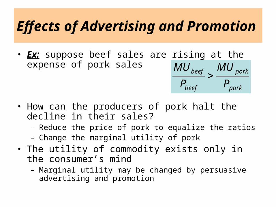
• Ex: suppose beef sales are rising at the expense of pork sales

• How can the producers of pork halt the decline in their sales?– Reduce the price of pork to equalize the ratios– Change the marginal utility of pork

• The utility of commodity exists only in the consumer’s mind– Marginal utility may be changed by persuasive advertising and

promotion

pork

pork

beef

beef

P

MU

P

MU

Marginal Utility and Demand Curves

• A consumer’s demand curve can be derived from marginal utility data

• E.g.:

• MUM=2; MUX= 200 – 4QX

• Calculating of price from information on marginal utility of commodity X and marginal utility of money

M

XX MU

MUP

The Ordinal Approach to Consumer Equilibrium

The Characteristics of the Consumer’s Preferences• Given three bundles of goods (A, B, and C), if an

individual prefers A to B and B to C, he must prefer A to C– If an individual is indifferent between A and B and between B

and C, he must be indifferent between A and C

• If an individual can rank any pair of bundles chosen at random from all conceivable bundles, he can rank all conceivable bundles

• If bundle A contains at least as many units of each commodity as bundle B, and more units of at least one commodity, A must be preferred to B

Indifference Curves

• Def.: An indifference curve is the set of all combinations of commodities X and Y that yield the same level of total utility or satisfaction

– An indifference map is a graph that shows a set of indifference curves

Characteristics of Indifference Curves

• They are infinite in number and every point in the commodity space lies on an indifference curve

• They are continuous and downward sloping

• They are concave from above (convex to the origin)

• The farther away from the origin an indifference curve is, the higher the level of utility it represents

• They cannot intersect, since each curve represents a different and unique level of utility

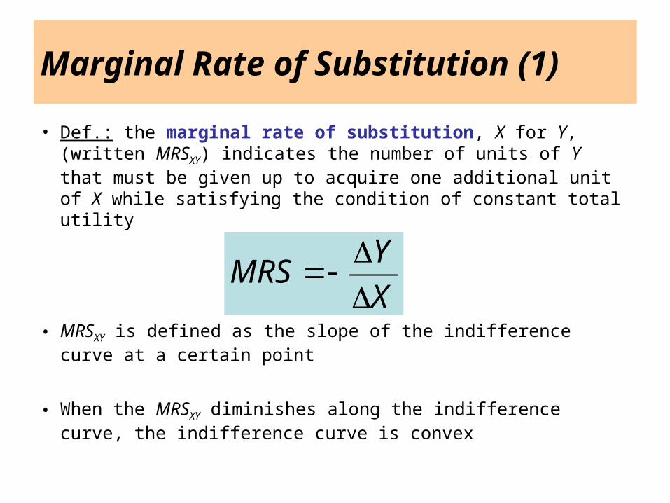
Marginal Rate of Substitution (1)

• Def.: the marginal rate of substitution, X for Y, (written MRSXY) indicates the number of units of Y that must be given up to acquire one additional unit of X while satisfying the condition of constant total utility

• MRSXY is defined as the slope of the indifference curve at a certain point

• When the MRSXY diminishes along the indifference curve, the indifference curve is convex

X

YMRS

Perfect Substitutes and Perfect Complements• The two goods are perfect substitutes when the

marginal rate of substitution of one good for another is a constant– The indifference curves are straight lines

• The two goods are perfect complements when the marginal rate of substitution of one good for another is infinite– The indifference curves are shaped as right angles

The Budget Line

• Def.: the budget line or line of attainable combinations is the set of all combinations of commodities X and Y that can be purchased when all available income is spent on X and Y

• Relationship between MU and MRSXY

• MRSXY and the exchange of goods

Marginal Rate of Substitution (2)

Consumer Equilibrium

• Utility maximization is achieved when the budget is allocated so that the marginal utility per dollar of expenditure is the same for each good

Y

Y

X

X

P

MU

P

MU

Individual Demand

• Price-consumption curve for X– Traces the utility-maximizing combinations of goods X and Y

associated with each and every price of good X

• The demand curve relates the quantity of good X that the consumer will buy to the price of X– The lower the price of the product, the higher the level of utility– At every point at the demand curve, the consumer is maximizing

utility

• Ordinary vs. Giffen goods

Income Changes

• Income-consumption curve– Traces the utility-maximizing combinations of goods X and Y

associated with different levels of income

• Engel curves– Relate the quantity of a good consumed to income

• Normal vs. inferior goods