Khushal Khan Khattak Armaghan-e-Khushal Baz Nama, Fazal Nama, Distar Nama and Farrah Nama
Upload
dinhkhuongCategory
view
226download
1
Sched-MAC
Features
DescriptionNAMA, LAMA, PAMA
TRAMA
DYNAMMA
Comparison
PerformanceNAMA, LAMA, and PAMA
TRAMA
DYNAMMA
Comparison
Further Reading
BackupNAMA
TRAMA
Schedule-based MACs:NAMA, LAMA, PAMA
and TRAMAand DYNAMMA
and a little of TRANSFORMA
presented by Vladislav Petkov
Department of Computer EngineeringUniversity of California, Santa Cruz
January 20, 2010 / CMPE257

Sched-MAC
Features
DescriptionNAMA, LAMA, PAMA
TRAMA
DYNAMMA
Comparison
PerformanceNAMA, LAMA, and PAMA
TRAMA
DYNAMMA
Comparison
Further Reading
BackupNAMA
TRAMA
Outline
Protocol Features
Protocol DescriptionNAMA, LAMA, PAMATRaffic Adaptive Medium AccessDYNamic Multi-channel Medium AccessComparison
Protocol PerformanceNAMA, LAMA, and PAMATRaffic Adaptive Medium AccessDYNamic Multi-channel Medium AccessOverall Comparison

Sched-MAC
Features
DescriptionNAMA, LAMA, PAMA
TRAMA
DYNAMMA
Comparison
PerformanceNAMA, LAMA, and PAMA
TRAMA
DYNAMMA
Comparison
Further Reading
BackupNAMA
TRAMA
Features of TRAMA, FLAMA and DYNAMMA
Common to all three! Schedule based data transmission! Energy-efficient! Use of 2-hop neighborhood information
TRAMA! Application
independent! Explicit
schedules! Single
channel
FLAMA! Designed for
sensor-networks
! Flow-based! Multi-channel
ready! Lightweight
DYNAMMA! Application
independent! Flow-based! Multi-channel
Sched-MAC
Features
DescriptionNAMA, LAMA, PAMA
TRAMA
DYNAMMA
Comparison
PerformanceNAMA, LAMA, and PAMA
TRAMA
DYNAMMA
Comparison
Further Reading
BackupNAMA
TRAMA
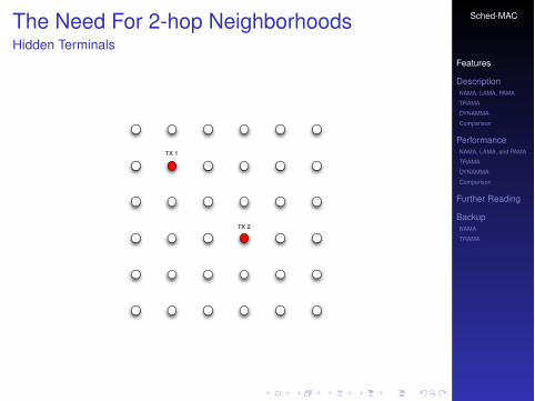
The Need For 2-hop NeighborhoodsHidden Terminals
TX 1
TX 2
Sched-MAC
Features
DescriptionNAMA, LAMA, PAMA
TRAMA
DYNAMMA
Comparison
PerformanceNAMA, LAMA, and PAMA
TRAMA
DYNAMMA
Comparison
Further Reading
BackupNAMA
TRAMA
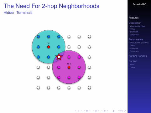
The Need For 2-hop NeighborhoodsHidden Terminals
TX 1
TX 2
Sched-MAC
Features
DescriptionNAMA, LAMA, PAMA
TRAMA
DYNAMMA
Comparison
PerformanceNAMA, LAMA, and PAMA
TRAMA
DYNAMMA
Comparison
Further Reading
BackupNAMA
TRAMA
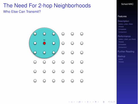
The Need For 2-hop NeighborhoodsWho Else Can Transmit?
TX

Sched-MAC
Features
DescriptionNAMA, LAMA, PAMA
TRAMA
DYNAMMA
Comparison
PerformanceNAMA, LAMA, and PAMA
TRAMA
DYNAMMA
Comparison
Further Reading
BackupNAMA
TRAMA
The Need For 2-hop NeighborhoodsThey Can
TX
one of green nodes can transmit concurrently with red node
Sched-MAC
Features
DescriptionNAMA, LAMA, PAMA
TRAMA
DYNAMMA
Comparison
PerformanceNAMA, LAMA, and PAMA
TRAMA
DYNAMMA
Comparison
Further Reading
BackupNAMA
TRAMA
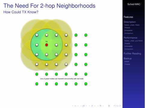
The Need For 2-hop NeighborhoodsHow Could TX Know?
TX
one of green nodes can transmit concurrently with red node

Sched-MAC
Features
DescriptionNAMA, LAMA, PAMA
TRAMA
DYNAMMA
Comparison
PerformanceNAMA, LAMA, and PAMA
TRAMA
DYNAMMA
Comparison
Further Reading
BackupNAMA
TRAMA
Outline
Protocol Features
Protocol DescriptionNAMA, LAMA, PAMATRaffic Adaptive Medium AccessDYNamic Multi-channel Medium AccessComparison
Protocol PerformanceNAMA, LAMA, and PAMATRaffic Adaptive Medium AccessDYNamic Multi-channel Medium AccessOverall Comparison
Sched-MAC
Features
DescriptionNAMA, LAMA, PAMA
TRAMA
DYNAMMA
Comparison
PerformanceNAMA, LAMA, and PAMA
TRAMA
DYNAMMA
Comparison
Further Reading
BackupNAMA
TRAMA
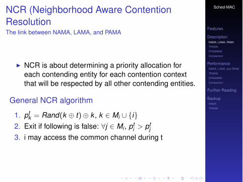
NCR (Neighborhood Aware ContentionResolutionThe link between NAMA, LAMA, and PAMA
! NCR is about determining a priority allocation foreach contending entity for each contention contextthat will be respected by all other contending entities.
General NCR algorithm
1. ptk = Rand(k ! t)! k , k " Mi # {i}
2. Exit if following is false: $j " Mi , pti > pt
j
3. i may access the common channel during t

Sched-MAC
Features
DescriptionNAMA, LAMA, PAMA
TRAMA
DYNAMMA
Comparison
PerformanceNAMA, LAMA, and PAMA
TRAMA
DYNAMMA
Comparison
Further Reading
BackupNAMA
TRAMA
Performance of NCR in generalA queuing theory analysis
Delay in System
0 0.05 0.1 0.15 0.2 0.25 0.3 0.35 0.4 0.45 0.50
10
20
30
40
50
60
qi=0.05
qi=0.10
qi=0.20
qi=0.50
Arrival Rate !i (Packet/Time Slot)
Del
ay in
Sys
tem
Ti (T
ime
Slot
s)
Average Packet Delays in the System
Figure 1: Average System Delay of Packets
queuing system at an entity i with di!erent channel accessprobability qi and arrival rate !i. To keep the queuing sys-tem in a steady state, it is necessary that !i < qi.
Because of the collision freedom of NCR, the common chan-nel can serve certain load up to the maximum channel ca-pacity. That is, the throughput over the common channel isthe summation of arrival rates at all competing entities aslong as the queuing system at each entity remains in equi-librium on the arrival and departure events. We have thefollowing system throughput S from each and every entityk that competes for the common channel:
S =k
min(!k, qk) (9)
where qk is the probability that k may access the commonchannel, and !k is the data packet arrival rate at k.
4. CHANNEL ACCESS PROTOCOLSFor simplicity, we abstract the topology of a packet radionetwork as an undirected graph G = (V, E). V is theset of nodes, each mounted with an omnidirectional radiotransceiver and assigned a unique ID number. E ! V "V isthe set of links between nodes. Unless notified otherwise, alink (u, v) # E indicates node u and v are within the trans-mission range of each other so that they can exchange radiopacket via the common channel, in which case the two nodesare called one-hop neighbors. Two distinct nodes having acommon one-hop neighbor are called two-hop neighbors toeach other. The set of d-hop neighbors of a specific node iis denoted by Nd
i , where d = 1, 2. Note that N1i $N2
i maynot be empty.
In multihop wireless networks, a single radio channel is spa-tially reused at di!erent parts of the network. Collisionshappen in three cases as illustrated in Figure 2 [23]. It issu"cient for collision-freedom if nodes within two hops donot transmit at the same time. Hence, contentions at a nodei should be resolved on the subgraph derived from the two-hop neighbors of i, i.e., N1
i % N2i , depending on node/link
activation schemes and signal coding methods as shown inthe following protocols.
(b) Direct Interference (c) Self Interference
(a) Hidden Terminal Problem
Figure 2: Examples of Collision Types
The following channel access protocols are described assum-ing that nodes already know their neighborhood, i.e., theyhave exchanged the necessary information about their two-hop neighborhood.
4.1 Node Activation ProtocolWe first present the NAMA (Node-Activation Multiple Ac-cess) protocol, which is based on NCR, node activation, anda distributed time division multiplexing scheme.
We do not address how nodes are time synchronized in thispaper. This can be achieved by either: (a) listening to datatra"c in the network, and aligning time slots to the lateststarting point of a complete packet transmission by one-hop neighbors; or (b) other means, such as GPS (globalpositioning systems) timing signals.
Membership SectionSection
Block
Part
0 1
0 1
0 1
S b
Tp-1
Ps -1
-1
Time Slot
Figure 3: Time Division in NAMA
A time slot is the smallest time unit for transmitting oneor more complete data packets. In NAMA, we impose morestructures on time slots such that the combination of Tp
consecutive time slots forms a part, Ps consecutive partsform a section, and Sb consecutive sections give the largestunit of time, block, as illustrated in Figure 3. Given thecurrent time slot number t, we derive the current time slotnumber of a part, the current part and section numbers asfollows:
t! = t mod Tp
p! = (t/Tp) mod Ps
s! = [t/(Tp " Ps)] mod Sb
(10)
where mod is a modular operator, and all operants are in-tegers.
A node i chooses only one part pi, during which to contendfor a time slot to transmit data packets. The choice of apart is dependent on the density of neighbors already usingthat part, usually decided when the node joins a network.
Throughput in System
! S =!
k
min(!k , qk )

Sched-MAC
Features
DescriptionNAMA, LAMA, PAMA
TRAMA
DYNAMMA
Comparison
PerformanceNAMA, LAMA, and PAMA
TRAMA
DYNAMMA
Comparison
Further Reading
BackupNAMA
TRAMA
Node Activation Multiple Access
Time Division Equations! t! = t mod Tp
! p! = (t/Tp) mod Ps
! s! = [t/(Tp ! Ps)] mod Sb
NAMA Algorithm1. Compute the current part number p! using
equations to the left
2. Exit if p! "= pi
3. Compute priority pti using NCR equation,
ptk = Rand(k # t)# k , k $ Mi % {i}
4. Assign node i to time slot ti = pti mod Tp
5. Compute the current time slot t! in part p!
using equations to the left
6. If ti "= t! then skip to step 10
7. Compute the set of contending neighborsMi = {k|k $ N1
i % N2i and pk = p! and (pt
kmod Tp) = t!}where pt
k is obtained from the NCR equationand pk is the part number chosen by node k
NAMA Algorithm (cont)8. Exit if NCR equation 2, &j $ Mi , pt
i > ptj ,
does not hold for i
9. Access the common channel in current timeslot t and exit
10. Exit if 'k, k $ N1i % N2
i and pk = p! and(pt
k mod Tp) = t!
11. The set of contending neighbors of node inow becomes:Mi = {k|k $ N1
i % N2i and pk = p!}
Compute another priority pt!k as follows:
pt!k = Rand(k # t # t!)# k, k $ Mi % {i}
12. Exit if 'j $ Mi , pt!i "> pt!
j
13. Access the common channel in time slot t
0 0.05 0.1 0.15 0.2 0.25 0.3 0.35 0.4 0.45 0.50
10
20
30
40
50
60
qi=0.05
qi=0.10
qi=0.20
qi=0.50
Arrival Rate !i (Packet/Time Slot)
Del
ay in
Sys
tem
Ti (T
ime
Slot
s)
Average Packet Delays in the System
Figure 1: Average System Delay of Packets
queuing system at an entity i with di!erent channel accessprobability qi and arrival rate !i. To keep the queuing sys-tem in a steady state, it is necessary that !i < qi.
Because of the collision freedom of NCR, the common chan-nel can serve certain load up to the maximum channel ca-pacity. That is, the throughput over the common channel isthe summation of arrival rates at all competing entities aslong as the queuing system at each entity remains in equi-librium on the arrival and departure events. We have thefollowing system throughput S from each and every entityk that competes for the common channel:
S =k
min(!k, qk) (9)
where qk is the probability that k may access the commonchannel, and !k is the data packet arrival rate at k.
4. CHANNEL ACCESS PROTOCOLSFor simplicity, we abstract the topology of a packet radionetwork as an undirected graph G = (V, E). V is theset of nodes, each mounted with an omnidirectional radiotransceiver and assigned a unique ID number. E ! V "V isthe set of links between nodes. Unless notified otherwise, alink (u, v) # E indicates node u and v are within the trans-mission range of each other so that they can exchange radiopacket via the common channel, in which case the two nodesare called one-hop neighbors. Two distinct nodes having acommon one-hop neighbor are called two-hop neighbors toeach other. The set of d-hop neighbors of a specific node iis denoted by Nd
i , where d = 1, 2. Note that N1i $N2
i maynot be empty.
In multihop wireless networks, a single radio channel is spa-tially reused at di!erent parts of the network. Collisionshappen in three cases as illustrated in Figure 2 [23]. It issu"cient for collision-freedom if nodes within two hops donot transmit at the same time. Hence, contentions at a nodei should be resolved on the subgraph derived from the two-hop neighbors of i, i.e., N1
i % N2i , depending on node/link
activation schemes and signal coding methods as shown inthe following protocols.
(b) Direct Interference (c) Self Interference
(a) Hidden Terminal Problem
Figure 2: Examples of Collision Types
The following channel access protocols are described assum-ing that nodes already know their neighborhood, i.e., theyhave exchanged the necessary information about their two-hop neighborhood.
4.1 Node Activation ProtocolWe first present the NAMA (Node-Activation Multiple Ac-cess) protocol, which is based on NCR, node activation, anda distributed time division multiplexing scheme.
We do not address how nodes are time synchronized in thispaper. This can be achieved by either: (a) listening to datatra"c in the network, and aligning time slots to the lateststarting point of a complete packet transmission by one-hop neighbors; or (b) other means, such as GPS (globalpositioning systems) timing signals.
Membership SectionSection
Block
Part
0 1
0 1
0 1
S b
Tp-1
Ps -1
-1
Time Slot
Figure 3: Time Division in NAMA
A time slot is the smallest time unit for transmitting oneor more complete data packets. In NAMA, we impose morestructures on time slots such that the combination of Tp
consecutive time slots forms a part, Ps consecutive partsform a section, and Sb consecutive sections give the largestunit of time, block, as illustrated in Figure 3. Given thecurrent time slot number t, we derive the current time slotnumber of a part, the current part and section numbers asfollows:
t! = t mod Tp
p! = (t/Tp) mod Ps
s! = [t/(Tp " Ps)] mod Sb
(10)
where mod is a modular operator, and all operants are in-tegers.
A node i chooses only one part pi, during which to contendfor a time slot to transmit data packets. The choice of apart is dependent on the density of neighbors already usingthat part, usually decided when the node joins a network.
Sched-MAC
Features
DescriptionNAMA, LAMA, PAMA
TRAMA
DYNAMMA
Comparison
PerformanceNAMA, LAMA, and PAMA
TRAMA
DYNAMMA
Comparison
Further Reading
BackupNAMA
TRAMA
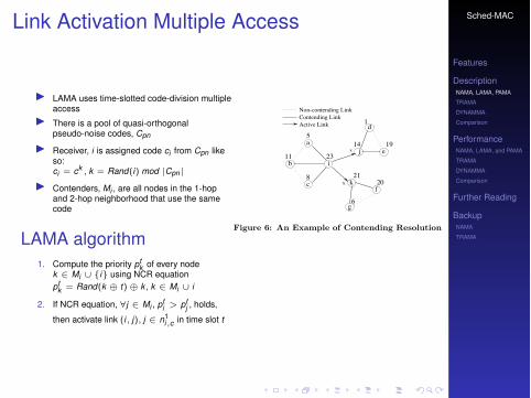
Link Activation Multiple Access
! LAMA uses time-slotted code-division multipleaccess
! There is a pool of quasi-orthogonalpseudo-noise codes, Cpn
! Receiver, i is assigned code ci from Cpn likeso:ci = ck , k = Rand(i) mod |Cpn|
! Contenders, Mi , are all nodes in the 1-hopand 2-hop neighborhood that use the samecode
LAMA algorithm1. Compute the priority pt
k of every nodek $ Mi % {i} using NCR equationpt
k = Rand(k # t)# k , k $ Mi % i
2. If NCR equation, &j $ Mi , pti > pt
j , holds,
then activate link (i, j), j $ n1i,c in time slot t
Because we have a limited number of pseudo-noise codes forassignment, it is possible that multiple nodes to share thesame code. If we denote the set of i’s one-hop neighborsassigned with code c as n1
i,c, our goal in LAMA is to decidewhether node i can activate a link on a code c and sendpacket to one of the receivers in n1
i,c during time slot t.Therefore, the set of contenders to node i includes one-hopneighbors of i and one-hop neighbors of nodes in the set n1
i,c
excluding node i itself, as shown in the following formula:
Mi = N1i !
k!n1i,c
N1k " {i}. (14)
LAMA:
1. Compute the priority ptk of every node k # Mi ! {i}
using Eq. (1).
2. If Eq. (2) holds, then activate link (i, j), j # n1i,c in
time slot t. !
e
f
g
i
a
b
c
d
23
5
8
1
21
19
11
14
6
20
j
kx
x
Non-contending LinkContending LinkActive Link
Figure 6: An Example of Contending Resolution
Figure 6 exemplifies a contention situation at node i duringtime slot t. The topology is an undirected graph. The num-ber beside each node represents the current priority of thenode. Node j and k happen to have the same code x. Todetermine if i can activate links on code x, we compare pri-orities of nodes according to LAMA. Node i has the highestpriority within one-hop neighbors, and higher priority thanj and k as well as their one-hop neighbors. Therefore, i canactivate either (i, j) or (i, k) in the current time slot t de-pending on back-logged data flows at i. In addition, nodee may activate link (e, d) if d is assigned a code other thancode x.
4.3 Pairwise Link Activation ProtocolThe PAMA (Pairwise-link Activation Multiple Access) pro-tocol is also a time-slotted link activation protocol based ona code division multiplexing scheme using DSSS. The dif-ference with LAMA is that a code is assigned for a giventransmitter-receiver pair, and computed every time-slot, sothat the contention situation is di!erent from time slot totime slot.
Unlike NAMA and LAMA in which contending entities arenodes, links are the entities competing for channel access
in PAMA. Links are directed in PAMA to signify transmis-sion directions. Each undirected link is represented by twodirected links in opposite directions.
As in LAMA, we assume a pool of quasi-orthogonal pseudo-noise codes, Cpn = {ck}. A pseudo-noise code cu from Cpn
is assigned to a directional link (u, v) at time slot t accordingto the following hashing function:
cu = ck, k = Rand(u$ t)$ u mod |Cpn|. (15)
Note that it is unnecessary to involve v in the code assign-ment, because of the simple fact that a node can activateonly one link at a time.
Like LAMA, the two-hop neighbor information is presumedto be available in PAMA by the appropriate integration ofNAMA and PAMA.
PAMA decides whether a directed link (u, v) can be acti-vated by node u in time slot t. The set of contenders to link(u, v) are the incident links of u and v excluding (u, v) itself,i.e.,
M(u,v) = {(x, y) | (x, y) # E,x # {u, v} }!{(x, y) | (x, y) # E, y # {u, v} }" {(u, v)}.
b c
ak
dk
Figure 7: An Example of Hidden Terminal ProblemIn PAMA
When a link (u, v) is activated, there are possible hidden ter-minal conflicts from one-hop neighbors of v if any outgoinglink on the one-hop neighbors of node v is assigned the samecode as (u, v). Figure 7 illustrates that a collision happensat node b when link (a, b) and (c, d) are activated using thesame code k. PAMA is able to deactivate link (a, b) for thecurrent time slot as described in the following algorithm:
PAMA:
1. Compute the priority pt(x,y) of every link (x, y) # M(u,v)!
{(u, v)} using Eq. (16):
pt(x,y) = Rand(x$ y $ t)$ x$ y (16)
2. Exit if Eq. (17) does not hold.
%(x, y) # M(u,v), pt(u,v) > pt
(x,y) (17)
3. Compute the priority of each two-hop neighbor of nodeu, that is:
ptk = Rand(k $ t)$ k, k # N2
u (18)
4. Compute the code assignment ck on node k, k # N2u
using Eq. (15).
5. Activate link (u, v) in time slot t if:
%k # N2u and cu = ck, pt
u > ptk (19)
!

Sched-MAC
Features
DescriptionNAMA, LAMA, PAMA
TRAMA
DYNAMMA
Comparison
PerformanceNAMA, LAMA, and PAMA
TRAMA
DYNAMMA
Comparison
Further Reading
BackupNAMA
TRAMA
Pairwise Activation Multiple Access
! In both NAMA and LAMA contending entities werenodes
! In PAMA, the contending entities are links! PAMA uses quasi-orthogonal pseudo-noise codes
like LAMA, but they are computed fortransmitter-receiver pairs
! PAMA is also time-slotted like NAMA and LAMA! I won’t go into the details of PAMA in the slides
Sched-MAC
Features
DescriptionNAMA, LAMA, PAMA
TRAMA
DYNAMMA
Comparison
PerformanceNAMA, LAMA, and PAMA
TRAMA
DYNAMMA
Comparison
Further Reading
BackupNAMA
TRAMA
Outline
Protocol Features
Protocol DescriptionNAMA, LAMA, PAMATRaffic Adaptive Medium AccessDYNamic Multi-channel Medium AccessComparison
Protocol PerformanceNAMA, LAMA, and PAMATRaffic Adaptive Medium AccessDYNamic Multi-channel Medium AccessOverall Comparison

Sched-MAC
Features
DescriptionNAMA, LAMA, PAMA
TRAMA
DYNAMMA
Comparison
PerformanceNAMA, LAMA, and PAMA
TRAMA
DYNAMMA
Comparison
Further Reading
BackupNAMA
TRAMA
TRAMAOverview
Scheduled Access Random Access
Switching Period
Signaling Slots
Transmission Slots
Figure 1: Time slot organization
Short Schedule Summary
SourceAddr DestAddr Timeout BitmapType NumSlots
b) Data Header
Type SourceAddr DestAddr DeleteNum AddNum Deleted NodeID’s Added NodeID’s
a) Signal Header
(
(
Figure 2: Signaling and data packet header for-mat
information to select the transmitters and receivers for thecurrent time slot, leaving all other nodes in liberty to switchto low-power mode.
TRAMA assumes a single, time-slotted channel for bothdata and signaling transmissions. Figure 1 shows the overalltime-slot organization of the protocol. Time is organized assections of random- and scheduled-access periods. We re-fer to random-access slots as signaling slots and scheduled-access slots as transmission slots. Because the data ratesof a sensor network are relatively low, the duration of timeslots is much larger than typical clock drifts. For exam-ple, for a 115.2 Kbps radio, we use a transmission slot ofapproximately 46ms to transmit 512-byte application layerdata units. Hence, clock drifts in the order of ms can be tol-erated, and yet typically clock drifts are in the order of mi-croseconds or even less. This allows very simple timestampmechanisms (e.g., [10]) to be used for node synchronization.When much smaller clock drifts must be assumed and moreexpensive nodes can be used, nodes can be time synchro-nized using techniques such as GPS [9]. Accordingly, in theremainder of our description of TRAMA, we simply assumethat adequate synchronization is attained.
NP propagates one-hop neighbor information among neigh-boring nodes during the random access period using thesignaling slots, to obtain consistent two-hop topology in-formation across all nodes. As the name suggests, duringthe random access period, nodes perform contention-basedchannel acquisition and thus signaling packets are proneto collisions.
Transmission slots are used for collision-free data exchangeand also for schedule propagation. Nodes use SEP to ex-change tra!c-based information, or schedules, with neigh-bors. Essentially, schedules contain current information ontra!c coming from a node, i.e., the set of receivers for thetra!c originating at the node. A node has to announceits schedule using SEP before starting actual transmissions.SEP maintains consistent schedule information across neigh-bors and updates the schedules periodically.
AEA selects transmitters and receivers to achieve collision-free transmission using the information obtained from NPand SEP. This is the case, because electing both the trans-mitter and the receiver(s) for a particular time slot is a ne-cessity to achieve energy e!ciency in a collision-free trans-mission schedule. Random transmitter selection leads to col-lisions, and electing the transmitters and not the receiversfor a given time slot leads to energy waste, because all theneighbors around a selected transmitter have to listen in theslot, even if they are not to receive any data. Furthermore,selecting a transmitter without regard to its tra!c leads
to low channel utilization, because the selected transmit-ter may not have any data to send to the selected receiver.Hence, AEA uses tra!c information (i.e., which sender hastra!c for which receivers) to improve channel utilization.
The length of a transmission slot is fixed based on thechannel bandwidth and data size. Signaling packets are usu-ally smaller than data packets and thus transmission slotsare typically set as a multiple of signaling slots to allow foreasy synchronization. In our implementation, transmissionslots are seven times longer than signaling slots.
2.2 Access Modes and the Neighbor ProtocolIn sensor networks, nodes may fail (e.g., power drained) or
new nodes may be added (e.g., additional sensors deployed).To accommodate topology dynamics, TRAMA alternatesbetween random- and scheduled access.
TRAMA starts in random access mode where each nodetransmits by selecting a slot randomly. Nodes can only jointhe network during random access periods. The duty cycleof random- versus scheduled access depends on the type ofnetwork. In more dynamic networks, random access periodsshould occur more often. In more static scenarios, the inter-val between random access periods could be larger, becausetopology changes need to be accommodated only occasion-ally. In the case of sensor networks, there is very little or nomobility, depending on the type of application. Hence, themain function of random access periods is to permit node ad-ditions and deletions. Time synchronization could be doneduring this period. During random access periods, all nodesmust be in either transmit or receive state, so they can sendout their neighborhood updates and receive updates fromneighbors. Hence, the duration of the random access periodplays a significant role in energy consumption.
During random access periods, signaling packets may belost due to collisions, which can lead to inconsistent neigh-borhood information across nodes. To guarantee consistentneighborhood information with some degree of confidence,the length of the random access period and the number ofretransmissions of signaling packets are set accordingly. In[4], it is shown that, for a network with an average of Ntwo-hop neighbors, the number of signaling packet retrans-missions should be 7 and the retransmission interval 1.44!Nto guarantee packet delivery of 99%. Thus, the length of therandom access period will then be 7 ! 1.44 ! N .
NP gathers neighborhood information by exchanging smallsignaling packets during the random access period. Fig-ure 2(a) shows the format of the header of a signaling packet.Signaling packets carry incremental neighborhood updatesand if there are no updates, signaling packets are sent as
Random access mode! Permits node additions/deletions! Contention based access! Sized according to how dynamic and
number of nodes! Neighbor Protocol runs in this mode
Scheduled accessmode
! Adaptive Election Algorithm
! Schedule Exchange Protocol
! Data transfer

Sched-MAC
Features
DescriptionNAMA, LAMA, PAMA
TRAMA
DYNAMMA
Comparison
PerformanceNAMA, LAMA, and PAMA
TRAMA
DYNAMMA
Comparison
Further Reading
BackupNAMA
TRAMA
TRAMAOne of Three Building Blocks: Neighbor Protocol
Scheduled Access Random Access
Switching Period
Signaling Slots
Transmission Slots
Figure 1: Time slot organization
Short Schedule Summary
SourceAddr DestAddr Timeout BitmapType NumSlots
b) Data Header
Type SourceAddr DestAddr DeleteNum AddNum Deleted NodeID’s Added NodeID’s
a) Signal Header
(
(
Figure 2: Signaling and data packet header for-mat
information to select the transmitters and receivers for thecurrent time slot, leaving all other nodes in liberty to switchto low-power mode.
TRAMA assumes a single, time-slotted channel for bothdata and signaling transmissions. Figure 1 shows the overalltime-slot organization of the protocol. Time is organized assections of random- and scheduled-access periods. We re-fer to random-access slots as signaling slots and scheduled-access slots as transmission slots. Because the data ratesof a sensor network are relatively low, the duration of timeslots is much larger than typical clock drifts. For exam-ple, for a 115.2 Kbps radio, we use a transmission slot ofapproximately 46ms to transmit 512-byte application layerdata units. Hence, clock drifts in the order of ms can be tol-erated, and yet typically clock drifts are in the order of mi-croseconds or even less. This allows very simple timestampmechanisms (e.g., [10]) to be used for node synchronization.When much smaller clock drifts must be assumed and moreexpensive nodes can be used, nodes can be time synchro-nized using techniques such as GPS [9]. Accordingly, in theremainder of our description of TRAMA, we simply assumethat adequate synchronization is attained.
NP propagates one-hop neighbor information among neigh-boring nodes during the random access period using thesignaling slots, to obtain consistent two-hop topology in-formation across all nodes. As the name suggests, duringthe random access period, nodes perform contention-basedchannel acquisition and thus signaling packets are proneto collisions.
Transmission slots are used for collision-free data exchangeand also for schedule propagation. Nodes use SEP to ex-change tra!c-based information, or schedules, with neigh-bors. Essentially, schedules contain current information ontra!c coming from a node, i.e., the set of receivers for thetra!c originating at the node. A node has to announceits schedule using SEP before starting actual transmissions.SEP maintains consistent schedule information across neigh-bors and updates the schedules periodically.
AEA selects transmitters and receivers to achieve collision-free transmission using the information obtained from NPand SEP. This is the case, because electing both the trans-mitter and the receiver(s) for a particular time slot is a ne-cessity to achieve energy e!ciency in a collision-free trans-mission schedule. Random transmitter selection leads to col-lisions, and electing the transmitters and not the receiversfor a given time slot leads to energy waste, because all theneighbors around a selected transmitter have to listen in theslot, even if they are not to receive any data. Furthermore,selecting a transmitter without regard to its tra!c leads
to low channel utilization, because the selected transmit-ter may not have any data to send to the selected receiver.Hence, AEA uses tra!c information (i.e., which sender hastra!c for which receivers) to improve channel utilization.
The length of a transmission slot is fixed based on thechannel bandwidth and data size. Signaling packets are usu-ally smaller than data packets and thus transmission slotsare typically set as a multiple of signaling slots to allow foreasy synchronization. In our implementation, transmissionslots are seven times longer than signaling slots.
2.2 Access Modes and the Neighbor ProtocolIn sensor networks, nodes may fail (e.g., power drained) or
new nodes may be added (e.g., additional sensors deployed).To accommodate topology dynamics, TRAMA alternatesbetween random- and scheduled access.
TRAMA starts in random access mode where each nodetransmits by selecting a slot randomly. Nodes can only jointhe network during random access periods. The duty cycleof random- versus scheduled access depends on the type ofnetwork. In more dynamic networks, random access periodsshould occur more often. In more static scenarios, the inter-val between random access periods could be larger, becausetopology changes need to be accommodated only occasion-ally. In the case of sensor networks, there is very little or nomobility, depending on the type of application. Hence, themain function of random access periods is to permit node ad-ditions and deletions. Time synchronization could be doneduring this period. During random access periods, all nodesmust be in either transmit or receive state, so they can sendout their neighborhood updates and receive updates fromneighbors. Hence, the duration of the random access periodplays a significant role in energy consumption.
During random access periods, signaling packets may belost due to collisions, which can lead to inconsistent neigh-borhood information across nodes. To guarantee consistentneighborhood information with some degree of confidence,the length of the random access period and the number ofretransmissions of signaling packets are set accordingly. In[4], it is shown that, for a network with an average of Ntwo-hop neighbors, the number of signaling packet retrans-missions should be 7 and the retransmission interval 1.44!Nto guarantee packet delivery of 99%. Thus, the length of therandom access period will then be 7 ! 1.44 ! N .
NP gathers neighborhood information by exchanging smallsignaling packets during the random access period. Fig-ure 2(a) shows the format of the header of a signaling packet.Signaling packets carry incremental neighborhood updatesand if there are no updates, signaling packets are sent as
! Gathers neighborhood information by exchangingsignaling packets.
! Neighbor information exchanged incrementally
Sched-MAC
Features
DescriptionNAMA, LAMA, PAMA
TRAMA
DYNAMMA
Comparison
PerformanceNAMA, LAMA, and PAMA
TRAMA
DYNAMMA
Comparison
Further Reading
BackupNAMA
TRAMA
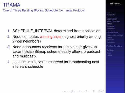
TRAMAOne of Three Building Blocks: Schedule Exchange Protocol
1. SCHEDULE_INTERVAL determined from application2. Node computes winning slots (highest priority among
2-hop neighbors)3. Node announces receivers for the slots or gives up
vacant slots (Bitmap scheme easily allows broadcastand multicast)
4. Last slot in interval is reserved for broadcasting nextinterval’s schedule

Sched-MAC
Features
DescriptionNAMA, LAMA, PAMA
TRAMA
DYNAMMA
Comparison
PerformanceNAMA, LAMA, and PAMA
TRAMA
DYNAMMA
Comparison
Further Reading
BackupNAMA
TRAMA
TRAMAOne of Three Building Blocks: Adaptive Election Algorithm
! Node u’s priority at time t determined by:prio(u, t) = hash(u ! t)
! This priority is used by the SEP to determine whichare the winning slots
! At any given time slot t , node u is in:! TX if u has highest priority in 2-hop hood and has
data to send! RX if it is intended receiver of the current transmitter! SL otherwise

Sched-MAC
Features
DescriptionNAMA, LAMA, PAMA
TRAMA
DYNAMMA
Comparison
PerformanceNAMA, LAMA, and PAMA
TRAMA
DYNAMMA
Comparison
Further Reading
BackupNAMA
TRAMA
Outline
Protocol Features
Protocol DescriptionNAMA, LAMA, PAMATRaffic Adaptive Medium AccessDYNamic Multi-channel Medium AccessComparison
Protocol PerformanceNAMA, LAMA, and PAMATRaffic Adaptive Medium AccessDYNamic Multi-channel Medium AccessOverall Comparison

Sched-MAC
Features
DescriptionNAMA, LAMA, PAMA
TRAMA
DYNAMMA
Comparison
PerformanceNAMA, LAMA, and PAMA
TRAMA
DYNAMMA
Comparison
Further Reading
BackupNAMA
TRAMA
DYNAMMAOverview
cess period all higher-layer data arrivals are queued and allnodes have their radios in transmit or receive state. Hence,longer random access periods lead to proportional increasein power consumption and buffer requirements. Further,the frequency of the random access period directly impactsthe amount of time needed for the network to re-configurewhenever there is a topology change. However, higher ran-dom access period frequency means longer data delivery de-lays.
In FLAMA, the transmission schedules are establishedbased on traffic flow information obtained during the ran-dom access period. This eliminates the overhead due toexplicit traffic schedule announcements and thus improveschannel utilization. However, the traffic characterizationmechanism used in FLAMA is specific to data gatheringapplications.
The limitations described above motivate the need forimproved topology and traffic discovery mechanisms that:(1) facilitate collision-free signaling exchange, (2) reducepower consumption and buffer size requirements, and still(3) allow for quick re-configuration and adaptability.
As described in detail in Section 3, DYNAMMA pro-vides a flexible, low-overhead, collision-free signalingmechanism for gathering topology and traffic information.Traffic, which is characterized by a set of directed flows,and topology information is exchanged periodically in or-der to adapt to topological and traffic pattern changes. DY-NAMMA’s distributed scheduling protocol then uses topol-ogy and traffic information to schedule collision-free trans-missions across multiple channels. Figure 1 illustrates thedifferent approaches in scheduled-access MAC time slot or-ganization.
Previous approaches to channel access scheduling, es-tablish transmission schedules by electing the highest prior-ity node as the transmitter. The intended receivers for theschedule are decided based on traffic schedule announce-ments [9] or by pre-establishing who the forwarding nodesare [8]. In DYNAMMA, application traffic is modeled us-ing directed flows that can be directly derived from thedestination-based queueing at the MAC layer. Each flow isrepresented by its arrival rate and its relationship with otherincoming flows as explained in Section 3.
The WiMedia MAC targets UWB-based PHY [14] bydefining a distributed, time-slotted medium access mech-anism [14]. All nodes transmit beacons periodically andthe medium access scheme is based on distributed reserva-tions. Applications that require guaranteed service rates cantake advantage of the reservation-based structure. However,static reservation-based approaches are not suited to appli-cations with variable service rate. Reservation-based ap-proaches may also lead to fairness problems and increasedoverhead in creating and maintaining reservations.
All previously mentioned protocols are designed to work
Figure 2. Time slot organization in DYNAMMA
with a single channel. Given that most commercially avail-able radios to-date provide multiple orthogonal channels,protocols should make use of this feature to schedule paral-lel transmissions within a two-hop neighborhood, thus im-proving overall system capacity.
The remainder of this paper is organized as follows.Section 3 describes DYNAMMA in detail and Section 4presents performance results for DYNAMMA obtainedfrom simulations and testbed experimentation. Finally, inSection 5, we present concluding remarks and directions forfuture work.
3 DYNAMMA
We summarize the notations used in the description ofthe DYNAMMA framework in Table 1.
DYNAMMA’s time slot organization is illustrated in Fig-ure 2. Time is divided into equally sized time units calledsuperframes. DYNAMMA’s superframe concept is similarto that of IEEE 802.15.3 [5] and WiMedia MAC [14].
Every superframe consists of a fixed number of timeslots. DYNAMMA’s time slots can be of three differenttypes, namely: signaling slots, base data slots and burstdata slots. Signaling slots are used for neighbor/traffic in-formation exchange, while base data slots and burst dataslots are used for data exchange. The channel used for com-munication is dynamically assigned for every base– or burstdata slot.
The duration of base data slots and burst data slots arefixed based on: the physical layer transmission rate, datapacket size, number of data packets to be transmitted withinthe burst, channel switching time, and radio turn-on time.The duration of a signaling slot is based on the maximumsignaling frame duration. The proposed superframe struc-ture provides ample support and flexibility for neighbor dis-covery, traffic adaptation, and dynamic radio mode controlto enable system-level energy optimizations.
3.1 Signaling Slot Assignment
Every node in a two-hop neighborhood is assigned itsown signaling slot for collision-free signaling informa-
! Dynamically adapts to traffic patterns! Collision-free multi channel operation! Minimum signaling overhead
Sched-MAC
Features
DescriptionNAMA, LAMA, PAMA
TRAMA
DYNAMMA
Comparison
PerformanceNAMA, LAMA, and PAMA
TRAMA
DYNAMMA
Comparison
Further Reading
BackupNAMA
TRAMA
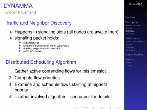
DYNAMMAFunctional Elements
Traffic and Neighbor Discovery
! Happens in signaling slots (all nodes are awake then)! signaling packet holds:
! superframe ID! location of signaling slot within superframe! one-hop neighborhood information! traffic information
Distributed Scheduling Algorithm
1. Gather active contending flows for this timeslot2. Compute flow priorities3. Examine and schedule flows starting at highest
priority4. ...rather involved algorithm - see paper for details

Sched-MAC
Features
DescriptionNAMA, LAMA, PAMA
TRAMA
DYNAMMA
Comparison
PerformanceNAMA, LAMA, and PAMA
TRAMA
DYNAMMA
Comparison
Further Reading
BackupNAMA
TRAMA
DYNAMMATraffic classification
Figure 3. Traffic classification
service rates. The number of channel access slots that aflow can contend is decided probabilistically based on itsclass identifier. In the current implementation we use threeflow classes, with class identifiers ranging from 0-2. Class 0flows are the highest-traffic flows and contend for all chan-nel access slots in the superframe. Class 1 and class 2 flowsare flows with reduced traffic and on average they contendfor one-half and one-quarter of the superframe, respectively.
All nodes maintain a set of destination-based queues(corresponding to outgoing flows), as shown in Figure 3.Flow classes are assigned based on the number of pack-ets in queue, the average service rate and average ar-rival rate in the previous superframe. The channel ac-cess probability of a flow ( f ) can be approximated as1/NumberO fContendingFlows. The expected number ofaccess slots for the flow, Er( f ) is computed as the productof the channel access probability of the flow and the num-ber of slots in the superframe. The required access slots forthe flow, Sr( f ) is computed based on the current MAC layerqueue parameters. Using the expected and required numberof access slots, the fractional usage, U( f ) = Sr( f )/Er( f ),is computed for all outgoing flows. Flow classes are thenassigned based on a threshold on the flow utilization fac-tor. A flow belongs to class p, if U( f ) > T Hp, where pis the smallest integer for which the inequality holds. Forthe current implementation, the class thresholds are fixed atTH0 = 0.95, T H1 = 0.65, and T H2 = 0.
Flow information is encoded in flow bitmap format to re-duce overhead in flow announcement. The position of theflow in the bitmap is used as the flow identifier and the bitis set to 1 to indicate that the flow exists. The originatingnode identifier and the flow identifier are used to uniquelyidentify a flow. The destinations for the flow are deter-mined based on the flow identifier and the ordering of theannounced one-hop neighbor list. The flow destinations areknown only for the one-hop neighbors, while the flow iden-tifier is known for both the one- and two-hop neighbors.
The most significant bit of the bitmap is reserved andis used to indicate a broadcast flow. Multicast destinationidentifiers are sent as an extension of the one-hop neigh-bor list and the corresponding bit positions are used for an-nouncing multicast flows.
Figure 4. Traffic discovery
The bit-width of the flow bitmap determines the maxi-mum number of flows that can be announced by a node.Figure 4 illustrates a simple out-flow bitmap and the corre-sponding node ordering for a node with two outgoing flows.
Nodes announce both their outgoing- and incoming(originating from a one-hop neighbor) flows. Additionally,nodes also announce all active outgoing flow identifiers oftheir two-hop neighbors (encoded as a bitmap). This pro-vides all the information required to uniquely identify atwo-hop originating flow and is required to avoid hiddenterminal collisions.
3.3 Distributed Scheduling Algorithm
Flow and neighborhood information gathered using thesignaling packet exchange are used by the distributedscheduling algorithm for establishing collision-free trans-mission schedules for base and burst data slots.
Whenever a new flow is added to the announcement, anode should ensure that the flow information is propagatedto the two-hop neighborhood before activating the flow fordistributed election and this can take up to two superframes.
At the start of the base data slot or burst data slot (sayt in superframe n), every node executes the election algo-rithm to determine its state as transmitter, receiver, or sleep-ing by electing flows from the set of contending flows. Thetransmission channel is determined using a pseudo-randomfunction (PRF). The algorithm ensures that the receivers ofthe elected flows are listening on the particular channel de-cided by the transmitter.
The steps involved in the election process at node u aredescribed below:
• Gather all active contending flows AF(u,t) for the cur-rent timeslot t. This includes all the outgoing flows ofnode u, all the outgoing flows of N1(u), and all the out-going flows of N2(u) that are currently active. Class 0flows are active for any timeslot t. For class 1 and class2 flows, a random number is generated using a pseudo-random function PRF( f low.srcId, t), which is used todecide if the flow contends in the current slot or not.
• Flow priorities are computed asPRF( f low.srcId, f low. f lowId,t,n) and the trans-
! Flows are put into the 3 classes depending on theirarrival and service rates

Sched-MAC
Features
DescriptionNAMA, LAMA, PAMA
TRAMA
DYNAMMA
Comparison
PerformanceNAMA, LAMA, and PAMA
TRAMA
DYNAMMA
Comparison
Further Reading
BackupNAMA
TRAMA
Outline
Protocol Features
Protocol DescriptionNAMA, LAMA, PAMATRaffic Adaptive Medium AccessDYNamic Multi-channel Medium AccessComparison
Protocol PerformanceNAMA, LAMA, and PAMATRaffic Adaptive Medium AccessDYNamic Multi-channel Medium AccessOverall Comparison

Sched-MAC
Features
DescriptionNAMA, LAMA, PAMA
TRAMA
DYNAMMA
Comparison
PerformanceNAMA, LAMA, and PAMA
TRAMA
DYNAMMA
Comparison
Further Reading
BackupNAMA
TRAMA
ComparisonDifferences and Similarities between TRAMA, FLAMA, and DYNAMMA
Figure 1. Various approaches in MAC time slot organization
2 State-of-the-Art
Existing MAC protocols can be categorized ascontention-, schedule-, or reservation-based. PAMAS [13]is one of the earliest contention-based proposals to addresspower efficiency in channel access. PAMAS saves energyby attempting to avoid over-hearing among neighboringnodes. To achieve this, PAMAS uses out-of channel sig-naling. Woo and Culler [19] address variations of CSMAtailored for sensor networks, and propose an adaptive ratecontrol mechanism to achieve fair bandwidth allocationamong sensor network nodes. In the power save (PS) modein IEEE 802.11 DCF, nodes sleep periodically. Tseng etal. [17] investigated three sleep modalities in 802.11 DCFin multi-hop networks. The sensor-MAC protocol [21], orS-MAC, exhibits similar functionality to that of PAMASand the protocol by Tseng et al.. Like the other approaches,S-MAC avoids overhearing and nodes periodically sleep.However, unlike PAMAS, S-MAC uses in-line signaling,and unlike modalities of the PS mode in 802.11 DCF,neighboring nodes can synchronize their sleep schedules.T-MAC [18] is an improvement over S-MAC that adaptsthe duty cycle based on traffic. However, synchronizedlisten periods increase channel contention significantly andalso increases the overall noise floor during transmissionsleading to degradation in link quality.
D-MAC [7] is a contention-based medium access pro-tocol optimized for data gathering applications over unidi-rectional trees. It schedules transmissions at each hop sothat the latency in data collection is reduced. However, D-MAC assumes fixed topology and does not allow multipledata gathering trees. It cannot adapt to other sensor networkapplications. All of the above mentioned protocols improveenergy efficiency by avoiding idle listening. However, theywaste energy in (1) collisions due to hidden terminals and(2) carrier-sensing.
In scheduled-access MACs, all nodes are time synchro-nized and access the medium using well-defined transmis-sion schedules. Thus, Scheduled-access MACs [2,8,10–12]have become an attractive approach to medium access inMANETs due to their potential for improving channel effi-ciency and increasing energy savings.
The Traffic-Adaptive Medium Access (TRAMA) proto-col [10] was the first proposal to implement energy-awareschedule-based medium access. TRAMA addresses energyefficiency by having nodes going into sleep mode if they arenot selected to transmit and are not the intended receivers oftraffic during a particular time slot. Besides its energy effi-ciency benefits, TRAMA’s use of traffic information alsomakes it adaptive to the application at hand. However,TRAMA’s adaptiveness comes at a price, namely the com-plexity of its election algorithm and scheduling overheadfor announcing traffic information. It should be noted thatschedule-based protocols exhibit inherently higher deliv-ery delays when compared to contention-based approaches.In TRAMA, this is exacerbated by the need to propagateschedule information.
Unlike TRAMA [10]), FLAMA [8] does not require ex-plicit schedule announcements during scheduled access pe-riods. Alternatively, application-specific traffic informationis exchanged among nodes during random access to reflectthe driving application’s specific traffic patterns, or flows.This allows FLAMA to still adapt to changes in traffic be-havior and topology (e.g., node failure).
In both TRAMA and FLAMA, topology informationis gathered during the random access period by exchang-ing signaling packets. Signaling exchange is based oncontention-based channel access and is prone to collisionsdue to hidden terminals. As topology information is criticalto establish collision-free transmission schedules, the ran-dom access period should be long enough to accommodatesignaling packet retransmissions. During the random ac-
Sched-MAC
Features
DescriptionNAMA, LAMA, PAMA
TRAMA
DYNAMMA
Comparison
PerformanceNAMA, LAMA, and PAMA
TRAMA
DYNAMMA
Comparison
Further Reading
BackupNAMA
TRAMA
Outline
Protocol Features
Protocol DescriptionNAMA, LAMA, PAMATRaffic Adaptive Medium AccessDYNamic Multi-channel Medium AccessComparison
Protocol PerformanceNAMA, LAMA, and PAMATRaffic Adaptive Medium AccessDYNamic Multi-channel Medium AccessOverall Comparison

Sched-MAC
Features
DescriptionNAMA, LAMA, PAMA
TRAMA
DYNAMMA
Comparison
PerformanceNAMA, LAMA, and PAMA
TRAMA
DYNAMMA
Comparison
Further Reading
BackupNAMA
TRAMA
NAMA, LAMA, and PAMA performanceFully-connected Network
0 0.1 0.2 0.3 0.4 0.50
50
100
150
200
Arrival Rate !i (Packet/Slot)
Del
ay T
i (Tim
e Sl
ot)
qi=0.5, 2 Nodes
NAMA LAMA PAMA Theory
0 0.05 0.1 0.15 0.2 0.250
50
100
150
200
Arrival Rate !i (Packet/Slot)
Del
ay T
i (Tim
e Sl
ot)
qi=0.2, 5 Nodes
0 0.05 0.1 0.15 0.20
50
100
150
200
250
300
Arrival Rate !i (Packet/Slot)
Del
ay T
i (Tim
e Sl
ot)
qi=0.1, 10 Nodes
0 0.02 0.04 0.06 0.08 0.10
50
100
150
200
250
300
Arrival Rate !i (Packet/Slot)
Del
ay T
i (Tim
e Sl
ot)
qi=0.05, 20 Nodes
Figure 9: Average Packet Delays In Fully-Connected Networks
access protocols that experience great loss in the through-put when the network load goes beyond certain point. No-tice that PAMA allows higher sustainable load in the sys-tem than NAMA and LAMA because PAMA allows channelreuse even when the topology is fully connected.
0 0.2 0.4 0.60
0.5
1
1.5
Arrival Rate !i (Packet/Slot)
Thro
ughp
ut S
(Pac
ket/S
lot)
qi=0.5, 2 Nodes
NAMA LAMA PAMA Theory
0 0.1 0.2 0.30
0.5
1
1.5
Arrival Rate !i (Packet/Slot)
Thro
ughp
ut S
(Pac
ket/S
lot)
qi=0.2, 5 Nodes
0 0.1 0.2 0.30
0.5
1
1.5
2
2.5
3
Arrival Rate !i (Packet/Slot)
Thro
ughp
ut S
(Pac
ket/S
lot)
qi=0.1, 10 Nodes
0 0.05 0.1 0.15 0.2 0.250
1
2
3
4
Arrival Rate !i (Packet/Slot)
Thro
ughp
ut S
(Pac
ket/S
lot)
qi=0.05, 20 Nodes
Figure 10: Packet Throughput Of Fully-ConnectedNetworks
6.2.2 Multihop Network Scenario:Figure 11 and 12 show the delay and throughput features ofthe three protocols in multihop networks. The networks aregenerated by randomly placing 100 nodes within an area of1000!1000 square meters. To simulate infinite plane thathas constant node placement density, the opposite sides ofthe square are seamed together, which visually turns thesquare area into a torus. By setting the transmission rangesof the transceiver on each node to 100, 200, 300, 400 me-ters, respectively, we also virtually change the topology andcontention levels in each case.
0 0.05 0.1 0.15 0.20
50
100
150
200
250
300
Arrival Rate !i (Packet/Slot)
Del
ay T
i (Tim
e Sl
ot)
Transmission Range=100
0 0.05 0.10
100
200
300
400
500
Arrival Rate !i (Packet/Slot)
Del
ay T
i (Tim
e Sl
ot)
Transmission Range=200
0 0.02 0.04 0.060
200
400
600
800
1000
Arrival Rate !i (Packet/Slot)
Del
ay T
i (Tim
e Sl
ot)
Transmission Range=300
0 0.01 0.02 0.03 0.040
200
400
600
800
1000
1200
1400
Arrival Rate !i (Packet/Slot)
Del
ay T
i (Tim
e Sl
ot)
Transmission Range=400
NAMALAMAPAMA
Figure 11: Average Packet Delays In Multihop Net-works
0 0.1 0.2 0.3 0.4 0.50
5
10
15
20
25
30
Arrival Rate !i (Packet/Slot)
Thro
ughp
ut S
(Pac
ket/S
lot)
Transmission Range=100
0 0.05 0.1 0.15 0.2 0.250
5
10
15
20
Arrival Rate !i (Packet/Slot)
Thro
ughp
ut S
(Pac
ket/S
lot)
Transmission Range=200
0 0.05 0.1 0.150
2
4
6
8
10
Arrival Rate !i (Packet/Slot)
Thro
ughp
ut S
(Pac
ket/S
lot)
Transmission Range=300
0 0.02 0.04 0.06 0.08 0.10
2
4
6
8
Arrival Rate !i (Packet/Slot)
Thro
ughp
ut S
(Pac
ket/S
lot)
Transmission Range=400
NAMALAMAPAMA
Figure 12: Packet Throughput Of Multihop Net-works
Figure 11 demonstrates the advantage of LAMA over NAMAbecause of improvements on channel reuse within two hopsof each node by applying code division multiplexing in LAMA.PAMA still gives higher starting point to delays than theother two even when network load is low due to similar rea-
0 0.1 0.2 0.3 0.4 0.50
50
100
150
200
Arrival Rate !i (Packet/Slot)
Del
ay T
i (Tim
e Sl
ot)
qi=0.5, 2 Nodes
NAMA LAMA PAMA Theory
0 0.05 0.1 0.15 0.2 0.250
50
100
150
200
Arrival Rate !i (Packet/Slot)
Del
ay T
i (Tim
e Sl
ot)
qi=0.2, 5 Nodes
0 0.05 0.1 0.15 0.20
50
100
150
200
250
300
Arrival Rate !i (Packet/Slot)
Del
ay T
i (Tim
e Sl
ot)
qi=0.1, 10 Nodes
0 0.02 0.04 0.06 0.08 0.10
50
100
150
200
250
300
Arrival Rate !i (Packet/Slot)
Del
ay T
i (Tim
e Sl
ot)
qi=0.05, 20 Nodes
Figure 9: Average Packet Delays In Fully-Connected Networks
access protocols that experience great loss in the through-put when the network load goes beyond certain point. No-tice that PAMA allows higher sustainable load in the sys-tem than NAMA and LAMA because PAMA allows channelreuse even when the topology is fully connected.
0 0.2 0.4 0.60
0.5
1
1.5
Arrival Rate !i (Packet/Slot)
Thro
ughp
ut S
(Pac
ket/S
lot)
qi=0.5, 2 Nodes
NAMA LAMA PAMA Theory
0 0.1 0.2 0.30
0.5
1
1.5
Arrival Rate !i (Packet/Slot)
Thro
ughp
ut S
(Pac
ket/S
lot)
qi=0.2, 5 Nodes
0 0.1 0.2 0.30
0.5
1
1.5
2
2.5
3
Arrival Rate !i (Packet/Slot)
Thro
ughp
ut S
(Pac
ket/S
lot)
qi=0.1, 10 Nodes
0 0.05 0.1 0.15 0.2 0.250
1
2
3
4
Arrival Rate !i (Packet/Slot)
Thro
ughp
ut S
(Pac
ket/S
lot)
qi=0.05, 20 Nodes
Figure 10: Packet Throughput Of Fully-ConnectedNetworks
6.2.2 Multihop Network Scenario:Figure 11 and 12 show the delay and throughput features ofthe three protocols in multihop networks. The networks aregenerated by randomly placing 100 nodes within an area of1000!1000 square meters. To simulate infinite plane thathas constant node placement density, the opposite sides ofthe square are seamed together, which visually turns thesquare area into a torus. By setting the transmission rangesof the transceiver on each node to 100, 200, 300, 400 me-ters, respectively, we also virtually change the topology andcontention levels in each case.
0 0.05 0.1 0.15 0.20
50
100
150
200
250
300
Arrival Rate !i (Packet/Slot)
Del
ay T
i (Tim
e Sl
ot)
Transmission Range=100
0 0.05 0.10
100
200
300
400
500
Arrival Rate !i (Packet/Slot)
Del
ay T
i (Tim
e Sl
ot)
Transmission Range=200
0 0.02 0.04 0.060
200
400
600
800
1000
Arrival Rate !i (Packet/Slot)
Del
ay T
i (Tim
e Sl
ot)
Transmission Range=300
0 0.01 0.02 0.03 0.040
200
400
600
800
1000
1200
1400
Arrival Rate !i (Packet/Slot)
Del
ay T
i (Tim
e Sl
ot)
Transmission Range=400
NAMALAMAPAMA
Figure 11: Average Packet Delays In Multihop Net-works
0 0.1 0.2 0.3 0.4 0.50
5
10
15
20
25
30
Arrival Rate !i (Packet/Slot)
Thro
ughp
ut S
(Pac
ket/S
lot)
Transmission Range=100
0 0.05 0.1 0.15 0.2 0.250
5
10
15
20
Arrival Rate !i (Packet/Slot)
Thro
ughp
ut S
(Pac
ket/S
lot)
Transmission Range=200
0 0.05 0.1 0.150
2
4
6
8
10
Arrival Rate !i (Packet/Slot)
Thro
ughp
ut S
(Pac
ket/S
lot)
Transmission Range=300
0 0.02 0.04 0.06 0.08 0.10
2
4
6
8
Arrival Rate !i (Packet/Slot)
Thro
ughp
ut S
(Pac
ket/S
lot)
Transmission Range=400
NAMALAMAPAMA
Figure 12: Packet Throughput Of Multihop Net-works
Figure 11 demonstrates the advantage of LAMA over NAMAbecause of improvements on channel reuse within two hopsof each node by applying code division multiplexing in LAMA.PAMA still gives higher starting point to delays than theother two even when network load is low due to similar rea-

Sched-MAC
Features
DescriptionNAMA, LAMA, PAMA
TRAMA
DYNAMMA
Comparison
PerformanceNAMA, LAMA, and PAMA
TRAMA
DYNAMMA
Comparison
Further Reading
BackupNAMA
TRAMA
NAMA, LAMA, and PAMA performanceMulti-hop Network
0 0.1 0.2 0.3 0.4 0.50
50
100
150
200
Arrival Rate !i (Packet/Slot)
Del
ay T
i (Tim
e Sl
ot)
qi=0.5, 2 Nodes
NAMA LAMA PAMA Theory
0 0.05 0.1 0.15 0.2 0.250
50
100
150
200
Arrival Rate !i (Packet/Slot)
Del
ay T
i (Tim
e Sl
ot)
qi=0.2, 5 Nodes
0 0.05 0.1 0.15 0.20
50
100
150
200
250
300
Arrival Rate !i (Packet/Slot)
Del
ay T
i (Tim
e Sl
ot)
qi=0.1, 10 Nodes
0 0.02 0.04 0.06 0.08 0.10
50
100
150
200
250
300
Arrival Rate !i (Packet/Slot)
Del
ay T
i (Tim
e Sl
ot)
qi=0.05, 20 Nodes
Figure 9: Average Packet Delays In Fully-Connected Networks
access protocols that experience great loss in the through-put when the network load goes beyond certain point. No-tice that PAMA allows higher sustainable load in the sys-tem than NAMA and LAMA because PAMA allows channelreuse even when the topology is fully connected.
0 0.2 0.4 0.60
0.5
1
1.5
Arrival Rate !i (Packet/Slot)
Thro
ughp
ut S
(Pac
ket/S
lot)
qi=0.5, 2 Nodes
NAMA LAMA PAMA Theory
0 0.1 0.2 0.30
0.5
1
1.5
Arrival Rate !i (Packet/Slot)
Thro
ughp
ut S
(Pac
ket/S
lot)
qi=0.2, 5 Nodes
0 0.1 0.2 0.30
0.5
1
1.5
2
2.5
3
Arrival Rate !i (Packet/Slot)
Thro
ughp
ut S
(Pac
ket/S
lot)
qi=0.1, 10 Nodes
0 0.05 0.1 0.15 0.2 0.250
1
2
3
4
Arrival Rate !i (Packet/Slot)
Thro
ughp
ut S
(Pac
ket/S
lot)
qi=0.05, 20 Nodes
Figure 10: Packet Throughput Of Fully-ConnectedNetworks
6.2.2 Multihop Network Scenario:Figure 11 and 12 show the delay and throughput features ofthe three protocols in multihop networks. The networks aregenerated by randomly placing 100 nodes within an area of1000!1000 square meters. To simulate infinite plane thathas constant node placement density, the opposite sides ofthe square are seamed together, which visually turns thesquare area into a torus. By setting the transmission rangesof the transceiver on each node to 100, 200, 300, 400 me-ters, respectively, we also virtually change the topology andcontention levels in each case.
0 0.05 0.1 0.15 0.20
50
100
150
200
250
300
Arrival Rate !i (Packet/Slot)
Del
ay T
i (Tim
e Sl
ot)
Transmission Range=100
0 0.05 0.10
100
200
300
400
500
Arrival Rate !i (Packet/Slot)
Del
ay T
i (Tim
e Sl
ot)
Transmission Range=200
0 0.02 0.04 0.060
200
400
600
800
1000
Arrival Rate !i (Packet/Slot)
Del
ay T
i (Tim
e Sl
ot)
Transmission Range=300
0 0.01 0.02 0.03 0.040
200
400
600
800
1000
1200
1400
Arrival Rate !i (Packet/Slot)
Del
ay T
i (Tim
e Sl
ot)
Transmission Range=400
NAMALAMAPAMA
Figure 11: Average Packet Delays In Multihop Net-works
0 0.1 0.2 0.3 0.4 0.50
5
10
15
20
25
30
Arrival Rate !i (Packet/Slot)
Thro
ughp
ut S
(Pac
ket/S
lot)
Transmission Range=100
0 0.05 0.1 0.15 0.2 0.250
5
10
15
20
Arrival Rate !i (Packet/Slot)
Thro
ughp
ut S
(Pac
ket/S
lot)
Transmission Range=200
0 0.05 0.1 0.150
2
4
6
8
10
Arrival Rate !i (Packet/Slot)
Thro
ughp
ut S
(Pac
ket/S
lot)
Transmission Range=300
0 0.02 0.04 0.06 0.08 0.10
2
4
6
8
Arrival Rate !i (Packet/Slot)
Thro
ughp
ut S
(Pac
ket/S
lot)
Transmission Range=400
NAMALAMAPAMA
Figure 12: Packet Throughput Of Multihop Net-works
Figure 11 demonstrates the advantage of LAMA over NAMAbecause of improvements on channel reuse within two hopsof each node by applying code division multiplexing in LAMA.PAMA still gives higher starting point to delays than theother two even when network load is low due to similar rea-
0 0.1 0.2 0.3 0.4 0.50
50
100
150
200
Arrival Rate !i (Packet/Slot)
Del
ay T
i (Tim
e Sl
ot)
qi=0.5, 2 Nodes
NAMA LAMA PAMA Theory
0 0.05 0.1 0.15 0.2 0.250
50
100
150
200
Arrival Rate !i (Packet/Slot)
Del
ay T
i (Tim
e Sl
ot)
qi=0.2, 5 Nodes
0 0.05 0.1 0.15 0.20
50
100
150
200
250
300
Arrival Rate !i (Packet/Slot)
Del
ay T
i (Tim
e Sl
ot)
qi=0.1, 10 Nodes
0 0.02 0.04 0.06 0.08 0.10
50
100
150
200
250
300
Arrival Rate !i (Packet/Slot)
Del
ay T
i (Tim
e Sl
ot)
qi=0.05, 20 Nodes
Figure 9: Average Packet Delays In Fully-Connected Networks
access protocols that experience great loss in the through-put when the network load goes beyond certain point. No-tice that PAMA allows higher sustainable load in the sys-tem than NAMA and LAMA because PAMA allows channelreuse even when the topology is fully connected.
0 0.2 0.4 0.60
0.5
1
1.5
Arrival Rate !i (Packet/Slot)
Thro
ughp
ut S
(Pac
ket/S
lot)
qi=0.5, 2 Nodes
NAMA LAMA PAMA Theory
0 0.1 0.2 0.30
0.5
1
1.5
Arrival Rate !i (Packet/Slot)
Thro
ughp
ut S
(Pac
ket/S
lot)
qi=0.2, 5 Nodes
0 0.1 0.2 0.30
0.5
1
1.5
2
2.5
3
Arrival Rate !i (Packet/Slot)
Thro
ughp
ut S
(Pac
ket/S
lot)
qi=0.1, 10 Nodes
0 0.05 0.1 0.15 0.2 0.250
1
2
3
4
Arrival Rate !i (Packet/Slot)
Thro
ughp
ut S
(Pac
ket/S
lot)
qi=0.05, 20 Nodes
Figure 10: Packet Throughput Of Fully-ConnectedNetworks
6.2.2 Multihop Network Scenario:Figure 11 and 12 show the delay and throughput features ofthe three protocols in multihop networks. The networks aregenerated by randomly placing 100 nodes within an area of1000!1000 square meters. To simulate infinite plane thathas constant node placement density, the opposite sides ofthe square are seamed together, which visually turns thesquare area into a torus. By setting the transmission rangesof the transceiver on each node to 100, 200, 300, 400 me-ters, respectively, we also virtually change the topology andcontention levels in each case.
0 0.05 0.1 0.15 0.20
50
100
150
200
250
300
Arrival Rate !i (Packet/Slot)
Del
ay T
i (Tim
e Sl
ot)
Transmission Range=100
0 0.05 0.10
100
200
300
400
500
Arrival Rate !i (Packet/Slot)
Del
ay T
i (Tim
e Sl
ot)
Transmission Range=200
0 0.02 0.04 0.060
200
400
600
800
1000
Arrival Rate !i (Packet/Slot)
Del
ay T
i (Tim
e Sl
ot)
Transmission Range=300
0 0.01 0.02 0.03 0.040
200
400
600
800
1000
1200
1400
Arrival Rate !i (Packet/Slot)
Del
ay T
i (Tim
e Sl
ot)
Transmission Range=400
NAMALAMAPAMA
Figure 11: Average Packet Delays In Multihop Net-works
0 0.1 0.2 0.3 0.4 0.50
5
10
15
20
25
30
Arrival Rate !i (Packet/Slot)
Thro
ughp
ut S
(Pac
ket/S
lot)
Transmission Range=100
0 0.05 0.1 0.15 0.2 0.250
5
10
15
20
Arrival Rate !i (Packet/Slot)
Thro
ughp
ut S
(Pac
ket/S
lot)
Transmission Range=200
0 0.05 0.1 0.150
2
4
6
8
10
Arrival Rate !i (Packet/Slot)
Thro
ughp
ut S
(Pac
ket/S
lot)
Transmission Range=300
0 0.02 0.04 0.06 0.08 0.10
2
4
6
8
Arrival Rate !i (Packet/Slot)
Thro
ughp
ut S
(Pac
ket/S
lot)
Transmission Range=400
NAMALAMAPAMA
Figure 12: Packet Throughput Of Multihop Net-works
Figure 11 demonstrates the advantage of LAMA over NAMAbecause of improvements on channel reuse within two hopsof each node by applying code division multiplexing in LAMA.PAMA still gives higher starting point to delays than theother two even when network load is low due to similar rea-

Sched-MAC
Features
DescriptionNAMA, LAMA, PAMA
TRAMA
DYNAMMA
Comparison
PerformanceNAMA, LAMA, and PAMA
TRAMA
DYNAMMA
Comparison
Further Reading
BackupNAMA
TRAMA
Outline
Protocol Features
Protocol DescriptionNAMA, LAMA, PAMATRaffic Adaptive Medium AccessDYNamic Multi-channel Medium AccessComparison
Protocol PerformanceNAMA, LAMA, and PAMATRaffic Adaptive Medium AccessDYNamic Multi-channel Medium AccessOverall Comparison

Sched-MAC
Features
DescriptionNAMA, LAMA, PAMA
TRAMA
DYNAMMA
Comparison
PerformanceNAMA, LAMA, and PAMA
TRAMA
DYNAMMA
Comparison
Further Reading
BackupNAMA
TRAMA
Synthetic TrafficDelivery Ratio and Queuing Delay
We used Qualnet [3] as our simulation platform and wepresent the results for a variety of scenarios. The underlyingphysical layer model used for all the experiments was basedon the TR1000, a typical radio used in sensor networks. TheTR1000 [2], the radio used by the UC Berkeley Motes [1],are short range, low data-rate (a maximum of 115.2KBPS)radios with built-in support for low-power sleep state. Theaverage power consumption in transmit, receive and sleepmodes is 24.75mW , 13.5mW and 15µW , respectively. Themaximum transition time for switching is 20µS. The modu-lation type used in the physical layer is ASK and the receiverthreshold is !75dBm. Fifty nodes are uniformly distributedover a 500m x 500m area in all the experiments. The trans-mission range of each node is 100m and the topology is suchthat the nodes have 6 one-hop neighbors on average. Theaverage size of the two-hop neighborhood for this network is17 nodes. Two di!erent types of tra"c load are consideredin our study. We used a scenario in which node tra"c isstatistically generated based on a exponentially distributedinter-arrival time. We chose this to stress-test protocol per-formance for di!erent arrival rates. We also test TRAMA’sperformance when driven by data gathering applications,which are considered typical of sensor networks. Below, wedescribe these tra"c scenarios as well as other simulationparameters in detail.
4.1 Protocol ParametersIn both scenarios we fixed up the SCHEDULE INTERV AL to
be 100 transmission slots for TRAMA. The maximum size ofa signaling packet is fixed at 128 bytes which gives to a slotperiod of 6.82ms with guard time to take care of switching.Transmission slots are seven times longer than the signalingslots supporting a maximum data fragment size 896 bytes.The random access period is fixed to 72 transmission slotsand is repeated once every 10000 transmission slots.
S-MAC is a contention-based channel access protocol andit uses periodic sleep intervals to conserve energy. Sleepschedules are established using SY NC packets which areexchanged once every SY NC INTERV AL. The duty cycle de-termines the length of the sleep interval.
We set SY NC INTERV AL as 10sec and we varied the dutycycle (10% and 50%). All the nodes are time synchronizedand hence we favored S-MAC by allowing the listen andsleep periods synchronized across the entire network. Wealso observed that S-MAC needed larger time to set up thelisten/sleep schedules with the neighbor. This is because S-MAC does not have a proper neighbor discovery protocol,it has to rely on the SY NC packets for doing this. SY NCpackets are transmitted only once and are transmitted unre-liably. Hence, a large warmup time of 20sec is allowed for the
SINK DATA INITIATORS FORWARDERS
Corner Sink Center Sink Edge Initiators
Figure 6: Data gathering application
0
0.2
0.4
0.6
0.8
1
0 0.5 1 1.5 2 2.5
Perc
enta
ge r
eceiv
ed
Mean interarrival time (in seconds)
TRAMANAMA802.11CSMA
SMAC-10SMAC-50
(a) Unicast Tra"c
0
0.2
0.4
0.6
0.8
1
0 0.5 1 1.5 2 2.5
Perc
enta
ge r
eceiv
ed
Mean interarrival time (in seconds)
TRAMANAMA802.11CSMA
SMAC-10SMAC-50
(b) Broadcast Tra"c
Figure 7: Average packet delivery ratio for synthetictra!c
neighbor information to settle down. Because the queuingdelay for the scheduling-type MAC’s is higher, we allowedsome more time for delivering the queued packets beforeending the simulation. The simulation is run for 400sec andthe results are averaged over multiple runs.
4.2 Synthetic Data GenerationThe objective of this experiment is to measure the per-
formance of TRAMA when all the nodes in the networkgenerate tra"c based on some statistical distribution. Weused exponential inter-arrival for generating data and variedthe rate from 0.5 to 2.5 seconds. A neighbor is randomlyselected as a next-hop every time a node transmits a packet.We tested both unicast and broadcast data generation sep-arately. The performance metrics are:
• Average Packet Delivery Ratio: It is the ratio ofnumber of packets received to the number of packetssent averaged over all the nodes. For broadcast tra"ca packet is counted to be received only if it is receivedby all the one-hop neighbors.
• Percentage Sleep Time: It is the ratio of the num-ber of sleeping slots to the total number of slots aver-aged over the entire network.
0.001
0.01
0.1
1
10
100
0 0.5 1 1.5 2 2.5
Ave
rag
e d
ela
y (
in s
eco
nd
s)
Mean interarrival time (in seconds)
TRAMANAMA802.11CSMA
SMAC-10SMAC-50
(a) Unicast Tra!c
1e-05
0.0001
0.001
0.01
0.1
1
10
100
0 0.5 1 1.5 2 2.5
Ave
rag
e d
ela
y (
in s
eco
nd
s)
Mean interarrival time (in seconds)
TRAMANAMA802.11CSMA
SMAC-10SMAC-50
(b) Broadcast Tra!c
Figure 8: Average queuing delay for synthetic tra!c
• Average queuing Delay: Average delay for thepacket to be delivered to the receiver
• Average Sleep Interval: This is the average lengthof sleeping interval. This measures the number of ra-dio mode switching involved. Frequent switching canwaste energy due to the transient power consumptioninvolved in switching.4
4.3 Data-Gathering ApplicationWe assume a sink is collecting data from all the sensors
for these experiments. The sink sends out a broadcast queryrequesting data from all the sensors. The sensors respondback with the data, which are generated periodically to thesink. We implemented a simple reverse-path routing to for-ward the data from the sensors to the sink. Figure 6 showsthe three di"erent scenarios considered for this study. Data-collection node or sink is placed in the corner for the firstcase and in the middle for the second case.
All the sensors respond with periodically generated datain both cases. Because data aggregation [14] or groupingdata to minimize tra!c, are advantageous, we also emulateddata aggregation in a third case. Here, only the nodes at theedge generate tra!c and we assume that the nodes do data
4Measurements for 802.11 based radios are available in [12].
0.2
0.3
0.4
0.5
0.6
0.7
0.8
0.9
1
0 0.5 1 1.5 2 2.5
Pe
rce
nta
ge
sle
ep
tim
e
Mean interarrival time (in seconds)
TRAMA-bcastTRAMA-ucast
SMAC-10-bcastSMAC-10-ucastSMAC-50-bcastSMAC-50-ucast
(a) Percentage Energy Savings
0
50
100
150
200
250
300
0 0.5 1 1.5 2 2.5
Ave
rag
e le
ng
th o
f sle
ep
in
terv
al (in
mill
i-se
co
nd
s)
Mean interarrival time (in seconds)
TRAMA-bcastTRAMA-ucast
SMAC-10-bcastSMAC-10-ucastSMAC-50-bcastSMAC-50-ucast
(b) Average Sleep Interval
Figure 9: Energy savings and average sleep intervalfor synthetic tra!c
aggregation and appends its reading to the parent node.To measure performance in these experiments we use themetrics defined for the synthetic case. The average packetdelivery ratio is measured as the ratio of total number ofdata received by the sink to the total number of data sentby all the sensors, unlike the per-hop delivery ratio used forsynthetic tra!c generation.
5. SIMULATION RESULTS
5.1 Synthetic TrafficThe packet delivery ratio, average queuing delay, percent-
age of sleep time, and average length of sleep intervals forsynthetic tra!c scenarios are shown in Figure 7, Figure 8,Figure 9(a) and Figure 9(b), respectively. We present re-sults for S-MAC using two di"erent duty cycles, namely 50%and 10%. Our results indicate that, in general, schedule-based MACs based on NCR achieve better delivery thanIEEE802.11, CSMA and S-MAC. The main reason for theimprovement in delivery is the collision freedom guaran-teed at all times during data transmission. The e"ect ismore noticeable when all nodes generate broadcast tra!c.In CSMA, S-MAC and IEEE802.11, broadcasting is unreli-able and susceptible to hidden-terminal collisions. This re-

Sched-MAC
Features
DescriptionNAMA, LAMA, PAMA
TRAMA
DYNAMMA
Comparison
PerformanceNAMA, LAMA, and PAMA
TRAMA
DYNAMMA
Comparison
Further Reading
BackupNAMA
TRAMA
Synthetic TrafficEnergy savings
0.001
0.01
0.1
1
10
100
0 0.5 1 1.5 2 2.5
Avera
ge d
ela
y (
in s
econds)
Mean interarrival time (in seconds)
TRAMANAMA802.11CSMA
SMAC-10SMAC-50
(a) Unicast Tra!c
1e-05
0.0001
0.001
0.01
0.1
1
10
100
0 0.5 1 1.5 2 2.5
Avera
ge d
ela
y (
in s
econds)
Mean interarrival time (in seconds)
TRAMANAMA802.11CSMA
SMAC-10SMAC-50
(b) Broadcast Tra!c
Figure 8: Average queuing delay for synthetic tra!c
• Average queuing Delay: Average delay for thepacket to be delivered to the receiver
• Average Sleep Interval: This is the average lengthof sleeping interval. This measures the number of ra-dio mode switching involved. Frequent switching canwaste energy due to the transient power consumptioninvolved in switching.4
4.3 Data-Gathering ApplicationWe assume a sink is collecting data from all the sensors
for these experiments. The sink sends out a broadcast queryrequesting data from all the sensors. The sensors respondback with the data, which are generated periodically to thesink. We implemented a simple reverse-path routing to for-ward the data from the sensors to the sink. Figure 6 showsthe three di"erent scenarios considered for this study. Data-collection node or sink is placed in the corner for the firstcase and in the middle for the second case.
All the sensors respond with periodically generated datain both cases. Because data aggregation [14] or groupingdata to minimize tra!c, are advantageous, we also emulateddata aggregation in a third case. Here, only the nodes at theedge generate tra!c and we assume that the nodes do data
4Measurements for 802.11 based radios are available in [12].
0.2
0.3
0.4
0.5
0.6
0.7
0.8
0.9
1
0 0.5 1 1.5 2 2.5
Perc
enta
ge s
leep tim
e
Mean interarrival time (in seconds)
TRAMA-bcastTRAMA-ucast
SMAC-10-bcastSMAC-10-ucastSMAC-50-bcastSMAC-50-ucast
(a) Percentage Energy Savings
0
50
100
150
200
250
300
0 0.5 1 1.5 2 2.5
Avera
ge length
of sle
ep inte
rval (in m
illi-seconds)
Mean interarrival time (in seconds)
TRAMA-bcastTRAMA-ucast
SMAC-10-bcastSMAC-10-ucastSMAC-50-bcastSMAC-50-ucast
(b) Average Sleep Interval
Figure 9: Energy savings and average sleep intervalfor synthetic tra!c
aggregation and appends its reading to the parent node.To measure performance in these experiments we use themetrics defined for the synthetic case. The average packetdelivery ratio is measured as the ratio of total number ofdata received by the sink to the total number of data sentby all the sensors, unlike the per-hop delivery ratio used forsynthetic tra!c generation.
5. SIMULATION RESULTS
5.1 Synthetic TrafficThe packet delivery ratio, average queuing delay, percent-
age of sleep time, and average length of sleep intervals forsynthetic tra!c scenarios are shown in Figure 7, Figure 8,Figure 9(a) and Figure 9(b), respectively. We present re-sults for S-MAC using two di"erent duty cycles, namely 50%and 10%. Our results indicate that, in general, schedule-based MACs based on NCR achieve better delivery thanIEEE802.11, CSMA and S-MAC. The main reason for theimprovement in delivery is the collision freedom guaran-teed at all times during data transmission. The e"ect ismore noticeable when all nodes generate broadcast tra!c.In CSMA, S-MAC and IEEE802.11, broadcasting is unreli-able and susceptible to hidden-terminal collisions. This re-

Sched-MAC
Features
DescriptionNAMA, LAMA, PAMA
TRAMA
DYNAMMA
Comparison
PerformanceNAMA, LAMA, and PAMA
TRAMA
DYNAMMA
Comparison
Further Reading
BackupNAMA
TRAMA
Sensor ScenarioCorner Sink
We used Qualnet [3] as our simulation platform and wepresent the results for a variety of scenarios. The underlyingphysical layer model used for all the experiments was basedon the TR1000, a typical radio used in sensor networks. TheTR1000 [2], the radio used by the UC Berkeley Motes [1],are short range, low data-rate (a maximum of 115.2KBPS)radios with built-in support for low-power sleep state. Theaverage power consumption in transmit, receive and sleepmodes is 24.75mW , 13.5mW and 15µW , respectively. Themaximum transition time for switching is 20µS. The modu-lation type used in the physical layer is ASK and the receiverthreshold is !75dBm. Fifty nodes are uniformly distributedover a 500m x 500m area in all the experiments. The trans-mission range of each node is 100m and the topology is suchthat the nodes have 6 one-hop neighbors on average. Theaverage size of the two-hop neighborhood for this network is17 nodes. Two di!erent types of tra"c load are consideredin our study. We used a scenario in which node tra"c isstatistically generated based on a exponentially distributedinter-arrival time. We chose this to stress-test protocol per-formance for di!erent arrival rates. We also test TRAMA’sperformance when driven by data gathering applications,which are considered typical of sensor networks. Below, wedescribe these tra"c scenarios as well as other simulationparameters in detail.
4.1 Protocol ParametersIn both scenarios we fixed up the SCHEDULE INTERV AL to
be 100 transmission slots for TRAMA. The maximum size ofa signaling packet is fixed at 128 bytes which gives to a slotperiod of 6.82ms with guard time to take care of switching.Transmission slots are seven times longer than the signalingslots supporting a maximum data fragment size 896 bytes.The random access period is fixed to 72 transmission slotsand is repeated once every 10000 transmission slots.
S-MAC is a contention-based channel access protocol andit uses periodic sleep intervals to conserve energy. Sleepschedules are established using SY NC packets which areexchanged once every SY NC INTERV AL. The duty cycle de-termines the length of the sleep interval.
We set SY NC INTERV AL as 10sec and we varied the dutycycle (10% and 50%). All the nodes are time synchronizedand hence we favored S-MAC by allowing the listen andsleep periods synchronized across the entire network. Wealso observed that S-MAC needed larger time to set up thelisten/sleep schedules with the neighbor. This is because S-MAC does not have a proper neighbor discovery protocol,it has to rely on the SY NC packets for doing this. SY NCpackets are transmitted only once and are transmitted unre-liably. Hence, a large warmup time of 20sec is allowed for the
SINK DATA INITIATORS FORWARDERS
Corner Sink Center Sink Edge Initiators
Figure 6: Data gathering application
0
0.2
0.4
0.6
0.8
1
0 0.5 1 1.5 2 2.5
Pe
rce
nta
ge
re
ce
ive
d
Mean interarrival time (in seconds)
TRAMANAMA802.11CSMA
SMAC-10SMAC-50
(a) Unicast Tra"c
0
0.2
0.4
0.6
0.8
1
0 0.5 1 1.5 2 2.5
Pe
rce
nta
ge
re
ce
ive
d
Mean interarrival time (in seconds)
TRAMANAMA802.11CSMA
SMAC-10SMAC-50
(b) Broadcast Tra"c
Figure 7: Average packet delivery ratio for synthetictra!c
neighbor information to settle down. Because the queuingdelay for the scheduling-type MAC’s is higher, we allowedsome more time for delivering the queued packets beforeending the simulation. The simulation is run for 400sec andthe results are averaged over multiple runs.
4.2 Synthetic Data GenerationThe objective of this experiment is to measure the per-
formance of TRAMA when all the nodes in the networkgenerate tra"c based on some statistical distribution. Weused exponential inter-arrival for generating data and variedthe rate from 0.5 to 2.5 seconds. A neighbor is randomlyselected as a next-hop every time a node transmits a packet.We tested both unicast and broadcast data generation sep-arately. The performance metrics are:
• Average Packet Delivery Ratio: It is the ratio ofnumber of packets received to the number of packetssent averaged over all the nodes. For broadcast tra"ca packet is counted to be received only if it is receivedby all the one-hop neighbors.
• Percentage Sleep Time: It is the ratio of the num-ber of sleeping slots to the total number of slots aver-aged over the entire network.
duces broadcast delivery significantly when we increase theload as our results indicate. For IEEE802.11 and S-MAC,the RTS/CTS/DATA/ACK exchange for unicast tra!c im-proves delivery when compared to broadcast tra!c becauseit reduces hidden-terminal collisions by doing collision avoid-ance.
Schedule-based MACs, on the other hand, incur higheraverage queuing delays. We should point out that whenmeasuring average delay, we account for the delay of packetssuccessfully delivered. However, TRAMA and NAMA de-liver more packets than contention-based MACs and this willreduce the retransmissions at the higher layers. Hence, theend-to-end delay perceived by the application will be com-parable to that of contention-based protocols. The averagequeuing delay for TRAMA is higher than that of NAMA dueto the overhead involved in propagating scheduling informa-tion. Once every SCHEDULE INTERV AL, a transmission slotis used for announcing schedules. This decreases the e"ec-tive channel access probability for data transmission. Thisscenario is not a favorable scenario for tra!c-adaptive elec-tions, because the tra!c is homogeneous across the networkand all nodes periodically generate tra!c. The throughputof TRAMA is comparable with that of NAMA and is sig-nificantly better than contention-based protocols for bothunicast and broadcast tra!c scenarios. The performance ofthe only other energy-e!cient protocol, S-MAC is compara-ble with IEEE802.11 in terms of throughput. However, thedelay is slightly higher than that of IEEE802.11 or CSMAdue to the sleep periods, and it increases as the duty cycle ofthe listen periods is decreased. For a duty cycle of 50%, thedelay of S-MAC is smaller than that of IEEE802.11 for theunicast-data generation scenario. This is because S-MACfrequently switches between sleep and listen modes(averagesleep interval plotted in Figure 9(b) reflects this) for thatduty cycle. This is equivalent to a node being awake mostof the time, and the delay is less because S-MAC does nothave any contention resolution algorithm.
The energy savings of TRAMA depend mainly on the traf-fic pattern, while the energy savings of S-MAC are depen-dent on the duty cycle. The total energy savings dependon both percentage sleep time and average length of sleepinterval. Percentage sleep time metric does not account forthe performance loss that is possible due to frequent ra-dio mode switching. The average length of sleep intervalquantifies the amount of radio-mode switching involved. Ahigher value of average sleep length is preferred because thisimplies less radio-mode switching and hence more savings.The results indicate that the percentage of sleep time isless for broadcast tra!c when compared to unicast tra!c,which is intuitive. The percentage sleep time of S-MACincreases as the duty cycle decreases. The price paid fordecreasing the duty cycle is an increase in latency. Thethroughput decreases more steeply for a lower duty cycle astra!c increases. For the broadcast packets, a 50% duty cy-cle achieves less throughput than 10% duty cycle. Broadcastis done by plain carrier sensing and is more prone to hid-den terminal collisions. The timing structure for 512 bytesdata that favors low duty cycle as it reduces the channelcontention and hence the collisions are reduced. Note thata broadcast packet is counted as delivered ONLY if it isdelivered to all the neighbors.
Compared with TRAMA, S-MAC with 10% duty cycleexhibits higher percentage of sleeping time. But the aver-
0.1
0.2
0.3
0.4
0.5
0.6
0.7
0.8
0.9
1
2 4 6 8 10 12 14 16
Pe
rce
nta
ge
re
ce
ive
d
Packet generation interval (in seconds)
TRAMANAMA802.11CSMASMAC
(a) Average delivery ratio
0.001
0.01
0.1
1
10
100
2 4 6 8 10 12 14 16
Ave
rag
e d
ela
y (
in s
eco
nd
s)
Packet generation interval (in seconds)
TRAMANAMA802.11CSMASMAC
(b) Average queuing delay
Figure 10: Corner Sink
age length of sleep intervals is much lower for S-MAC whencompared to TRAMA. This reduces the overall energy sav-ings due to the overhead involved in mode switching. Thisis the case even though S-MAC is being favored by assum-ing that synchronized listen/sleep schedules are establishedacross the nodes due to the simulation setup. The perfor-mance of TRAMA is not a"ected by nodes joining at discreteintervals because it does not require any synchronization oflisten/sleep schedules.
In the subsequent experiments, we only consider S-MACwith 10% duty cycle, which has better performance thanwith a 50% duty cycle.
5.2 Sensor Network ApplicationWe tested the protocols using a sensor network data gath-
ering application. One of the nodes in the network is des-ignated as the sink and the sink starts sending a broadcastquery. All nodes receiving a non-duplicate query add thesender of the query as the next hop for data forwarding,establishing a reverse-shortest path tree with the sink nodeas the root. Figures 10(a), 11(a), and 12(a) show the av-erage packet delivery ratio for the corner sink, center sink,and edge sink scenarios respectively. Schedule-based MACprotocols outperform the contention-based MAC protocolsin all the cases. The delivery is highest for the scenarioin which the edge nodes are generating tra!c. This is be-

Sched-MAC
Features
DescriptionNAMA, LAMA, PAMA
TRAMA
DYNAMMA
Comparison
PerformanceNAMA, LAMA, and PAMA
TRAMA
DYNAMMA
Comparison
Further Reading
BackupNAMA
TRAMA
Sensor ScenarioCenter and Edge Sinks
0.1
0.2
0.3
0.4
0.5
0.6
0.7
0.8
0.9
1
2 4 6 8 10 12 14 16
Pe
rce
nta
ge
re
ce
ive
d
Packet generation interval (in seconds)
TRAMANAMA802.11CSMASMAC
(a) Average delivery ratio
0.0001
0.001
0.01
0.1
1
10
100
2 4 6 8 10 12 14 16
Ave
rag
e d
ela
y (
in s
eco
nd
s)
Packet generation interval (in seconds)
TRAMANAMA802.11CSMASMAC
(b) Average queuing delay
Figure 11: Center Sink
cause the overall load in the network is low and well withinthe capacity of the protocols. Delivery to the center sinkis slightly higher than when corner sink is used because thepackets need to go through fewer number of hops to reachthe sink. TRAMA performs much like NAMA and the de-crease in throughput due to scheduling overhead is overcomeby TRAMA’s adaptive scheduling approach. The averagedelivery ratio is nearly constant for contention-based proto-cols as the variation in the o!ered load is not high.
Figures 10(b), 11(b), and 12(b) show the average per-hop delay for all the protocols for the sensor scenarios.Contention-based protocols outperform scheduling-basedprotocols in terms of delay. This is due to the latency in-troduced by random scheduling. Finally we show the per-centage sleep time achieved by TRAMA and S-MAC in Fig-ure 13(a). The percentage of time nodes can be put to sleepincreases with decrease in tra"c load. The percentage sleeptime is quite high (as high as 85%) for the edge sink sce-nario which has the lowest load. Again the average lengthof the sleep interval is also the highest for this case. Thisclearly shows the benefit of TRAMA’s tra"c adaptabilitywhen compared to S-MAC. The average sleep interval ofTRAMA is significantly higher than that of S-MAC. Whencompared to the edge sink scenario, the percentage sleeptime is less for the center and corner sink scenarios due tothe increased load. In the corner sink case, data forwarded
0.1
0.2
0.3
0.4
0.5
0.6
0.7
0.8
0.9
1
2 4 6 8 10 12 14 16
Pe
rce
nta
ge
re
ce
ive
d
Packet generation interval (in seconds)
TRAMANAMA802.11CSMASMAC
(a) Average delivery ratio
0.0001
0.001
0.01
0.1
1
10
2 4 6 8 10 12 14 16
Ave
rag
e d
ela
y (
in s
eco
nd
s)
Packet generation interval (in seconds)
TRAMANAMA802.11CSMASMAC
(b) Average queuing delay
Figure 12: Edge Sink
by the nodes which are closer to the sink is heavier thandata forwarded by nodes farther away. This reduces sleeptime for these nodes and hence the overall percentage sleeptime is lesser than the case where the sink is in the center.This also applies to the average length of sleep period shownin Figure 13(b).
6. CONCLUSIONS
In this paper we presented TRAMA, a new energy-awarechannel access protocol for sensor networks. TRAMA usestra"c-based scheduling to avoid wasting slots when nodesdo not have data to send and to switch nodes to a low-powerstandby radio mode when they are not intended receivers oftra"c.
Through extensive simulations, we compared TRAMA’sperformance against a number of contention- and a schedule-based MACs. It is evident from the simulation results thatsignificant energy savings (since nodes can sleep for up to87% of the time) can be achieved by TRAMA depending onthe o!ered load. TRAMA also achieves higher throughput(around 40% over S-MAC and CSMA and around 20% for802.11) when compared to contention-based protocols sinceit avoids collisions due to hidden terminals.
In general, schedule-based MACs exhibit higher delaysthan contention-based MACs. TRAMA is well suited forapplications that are not delay sensitive but require high
0.1
0.2
0.3
0.4
0.5
0.6
0.7
0.8
0.9
1
2 4 6 8 10 12 14 16
Perc
enta
ge r
eceiv
ed
Packet generation interval (in seconds)
TRAMANAMA802.11CSMASMAC
(a) Average delivery ratio
0.0001
0.001
0.01
0.1
1
10
100
2 4 6 8 10 12 14 16
Avera
ge d
ela
y (
in s
econds)
Packet generation interval (in seconds)
TRAMANAMA802.11CSMASMAC
(b) Average queuing delay
Figure 11: Center Sink
cause the overall load in the network is low and well withinthe capacity of the protocols. Delivery to the center sinkis slightly higher than when corner sink is used because thepackets need to go through fewer number of hops to reachthe sink. TRAMA performs much like NAMA and the de-crease in throughput due to scheduling overhead is overcomeby TRAMA’s adaptive scheduling approach. The averagedelivery ratio is nearly constant for contention-based proto-cols as the variation in the o!ered load is not high.
Figures 10(b), 11(b), and 12(b) show the average per-hop delay for all the protocols for the sensor scenarios.Contention-based protocols outperform scheduling-basedprotocols in terms of delay. This is due to the latency in-troduced by random scheduling. Finally we show the per-centage sleep time achieved by TRAMA and S-MAC in Fig-ure 13(a). The percentage of time nodes can be put to sleepincreases with decrease in tra"c load. The percentage sleeptime is quite high (as high as 85%) for the edge sink sce-nario which has the lowest load. Again the average lengthof the sleep interval is also the highest for this case. Thisclearly shows the benefit of TRAMA’s tra"c adaptabilitywhen compared to S-MAC. The average sleep interval ofTRAMA is significantly higher than that of S-MAC. Whencompared to the edge sink scenario, the percentage sleeptime is less for the center and corner sink scenarios due tothe increased load. In the corner sink case, data forwarded
0.1
0.2
0.3
0.4
0.5
0.6
0.7
0.8
0.9
1
2 4 6 8 10 12 14 16
Perc
enta
ge r
eceiv
ed
Packet generation interval (in seconds)
TRAMANAMA802.11CSMASMAC
(a) Average delivery ratio
0.0001
0.001
0.01
0.1
1
10
2 4 6 8 10 12 14 16
Avera
ge d
ela
y (
in s
econds)
Packet generation interval (in seconds)
TRAMANAMA802.11CSMASMAC
(b) Average queuing delay
Figure 12: Edge Sink
by the nodes which are closer to the sink is heavier thandata forwarded by nodes farther away. This reduces sleeptime for these nodes and hence the overall percentage sleeptime is lesser than the case where the sink is in the center.This also applies to the average length of sleep period shownin Figure 13(b).
6. CONCLUSIONS
In this paper we presented TRAMA, a new energy-awarechannel access protocol for sensor networks. TRAMA usestra"c-based scheduling to avoid wasting slots when nodesdo not have data to send and to switch nodes to a low-powerstandby radio mode when they are not intended receivers oftra"c.
Through extensive simulations, we compared TRAMA’sperformance against a number of contention- and a schedule-based MACs. It is evident from the simulation results thatsignificant energy savings (since nodes can sleep for up to87% of the time) can be achieved by TRAMA depending onthe o!ered load. TRAMA also achieves higher throughput(around 40% over S-MAC and CSMA and around 20% for802.11) when compared to contention-based protocols sinceit avoids collisions due to hidden terminals.
In general, schedule-based MACs exhibit higher delaysthan contention-based MACs. TRAMA is well suited forapplications that are not delay sensitive but require high

Sched-MAC
Features
DescriptionNAMA, LAMA, PAMA
TRAMA
DYNAMMA
Comparison
PerformanceNAMA, LAMA, and PAMA
TRAMA
DYNAMMA
Comparison
Further Reading
BackupNAMA
TRAMA
Sensor ScenarioEnergy Savings
0.7
0.75
0.8
0.85
0.9
0.95
1
2 4 6 8 10 12 14 16
Pe
rce
nta
ge
sle
ep
tim
e
Average packet generation period (in seconds)
TRAMA-centerTRAMA-corner
TRAMA-edgeSMAC-edge
SMAC-cornerSMAC-edge
(a) Percentage Energy Savings
0
100
200
300
400
500
600
700
800
2 4 6 8 10 12 14 16
Ave
rag
e le
ng
th o
f sle
ep
in
terv
al (in
mill
i-se
co
nd
s)
Average packet generation period (in seconds)
TRAMA-centerTRAMA-corner
TRAMA-edgeSMAC-edge
SMAC-cornerSMAC-edge
(b) Average Sleep Interval
Figure 13: Energy savings and average sleep intervalfor sensor scenarios
delivery guarantees and energy e!ciency. A typical exam-ple is sensor networks used for periodic data collection andmonitoring applications. In summary, TRAMA achievesenergy-savings comparable to S-MAC with delivery guar-antees comparable to NAMA.
7. REFERENCES
[1] http://www.cs.berkeley.edu/ awoo/smartdust/.[2] Product specification,
http://www.rfm.com/products/data/tr1000.pdf.[3] Scalable networks, http://www.scalble-solutions.com.[4] L. Bao and J. Garcia-Luna-Aceves. Hybrid channel
access scheduling in ad hoc networks. Proc. IEEETenth International Conference on Network Protocols(ICNP), November 2002.
[5] L. Bao and J. J. Garcia-Luna-Aceves. A new approachto channel access scheduling for ad hoc networks. InThe seventh annual international conference on Mobilecomputing and networking 2001, pages 210–221, 2001.
[6] I. Chlamtac and A. Farago. Making transmissionschedules immune to topology changes in multi-hoppacket radio networks. IEEE/ACM Transactions onNetworking, 2(1):23–29, February 1994.
[7] I. Chlamtac and A. Lerner. Fair algorithms formaximal link activation in multihop radio networks.
IEEE Transactions on Communications,35(7):739–746.
[8] I. Cidon and M. Sidi. Distributed assignmentalgorithms for multihop packet radio networks. IEEETransactions on Computers, 38(10):1236–1361,October 1989.
[9] E.D.Kaplan. Understanding GPS: Principles andApplications. Artech House, 1996.
[10] J. Elson and D. Estrin. Time synchronization forwireless sensor networks. In IPDPS 2001, April 2001.
[11] A. Ephremides and T. Truong. Scheduling broadcastsin multihop radio networks. IEEE Transactions onCommunications, 38(4):456–460, April 1990.
[12] L. M. Feeney and M. Nilsson. Investigating the energyconsumption of a wireless network interface in an adhoc networking environment. In IEEE INFOCOM,2001.
[13] IEEE. Wireless LAN medium access control (MAC)and physical layer specifications. ANSI/IEEEStandard 802.11, 1999 Edition, 1999.
[14] C. Intanagonwiwat, D. Estrin, R. Govindan, andJ. Heidemann. Impact of network density on dataaggregation in wireless sensor networks, 2001.
[15] J. Ju and V. Li. An optimal topology-transparentscheduling method in multihop packet radio networks.IEEE/ACM Transactions on Networking,6(3):298–306, June 1998.
[16] L. Kleirock and F. Tobagi. Packet switching in radiochannels, part 1: Carrier sense multiple-access modelsand their throughput-delay characteristics. IEEETransactions on Communications, 23(12):1400–1416.
[17] L. Kleirock and F. Tobagi. Packet switching in radiochannels, part 2: Hidden-terminal problem in carriersense multiple access and the busy-tone solution.IEEE Transactions on Communications,23(12):1417–1433, 1975.
[18] S. Lam. A carrier sense multiple access protocol forlocal networks. Computer Networks, 4:21–32, 1980.
[19] S. Ramanathan. A unified framework and algorithmfor channel assignment in wireless networks. WirelessNetworks, 5(2):81–94, 1999.
[20] S. Singh and C. Raghavendra. PAMAS: Power awaremulti-access protocol with signaling for ad hocnetworks, 1999.
[21] K. Sohrabi and G. Pottie. Performance of a novelself-organization protocol for wireless ad hoc sensornetworks. IEEE 50th. Vehicular TechnologyConference, pages 1222–1226, 1999.
[22] Y.-C. Tseng, C.-S. Hsu, and T.-Y. Hsieh.Power-saving protocols for IEEE 802.11-basedmulti-hop ad hoc networks. In Proceedings of theIEEE Infocom, June 2002.
[23] A. Woo and D. Culler. A transmission control schemefor media access in sensor networks. ACM/IEEEInternational Conference on Mobile Computing andNetworking (Mobicom) 2001, 2001.
[24] W. Ye, J. Heidemann, and D. Estrin. Anenergy-e!cient MAC protocol for wireless sensornetworks. IEEE Infocom 2002, pages 1567–1576, June2002.

Sched-MAC
Features
DescriptionNAMA, LAMA, PAMA
TRAMA
DYNAMMA
Comparison
PerformanceNAMA, LAMA, and PAMA
TRAMA
DYNAMMA
Comparison
Further Reading
BackupNAMA
TRAMA
Outline
Protocol Features
Protocol DescriptionNAMA, LAMA, PAMATRaffic Adaptive Medium AccessDYNamic Multi-channel Medium AccessComparison
Protocol PerformanceNAMA, LAMA, and PAMATRaffic Adaptive Medium AccessDYNamic Multi-channel Medium AccessOverall Comparison

Sched-MAC
Features
DescriptionNAMA, LAMA, PAMA
TRAMA
DYNAMMA
Comparison
PerformanceNAMA, LAMA, and PAMA
TRAMA
DYNAMMA
Comparison
Further Reading
BackupNAMA
TRAMA
Synthetic and Data Gathering TrafficAverage Delivery Ratio and Queuing Delay
cess period is fixed to 10000 signaling slots (0.2825s) andis repeated once every 10000 transmission slots (6.3075s).TRAMA incurs overhead due to random access period ev-ery 6.3075s and no data communication takes place duringthis interval. This can lead to increased queueing drops inTRAMA during random access period.
4.2 Simulation Results
4.2.1 Synthetic Traffic
In this scenario, all nodes generate unicast traffic to a ran-domly selected next-hop node. The data generation inter-val is varied from 1ms to 12ms and the results are averagedover several runs. Figure 7(a) shows the average packet de-livery ratio at each node and Figure 7(b) shows the averageper-hop queuing delay. The main observation here is thatthe major source of packet loss in scheduled-access MACprotocols is packet drops due to buffer overflows whereaspacket losses in 802.11 are mostly due to hidden terminalcollisions. Hence, packet delivery ratio decreases with in-creased offered load for all the protocols. Due to collision-freedom, both TRAMA and DYNAMMA exhibit higher de-livery ratio than the 802.11.
DYNAMMA with single channel (DYNAMMA-1)achieves better queueing delay when compared to TRAMAand this leads to improved delivery ratio. This is a consid-erable improvement given that one of the main drawbacksof scheduled-access MACs is their inherent queuing delay.This is why DYNAMMA’s queuing delay is higher than thatof the 802.11.
As we increase the number of channels (DYNAMMA-2 and DYNAMMA-3 for 2– and 3 channels, respectively),there is an improvement in the delivery ratio and queuingdelay, more pronounced when the offered traffic is high.However, we noticed that as we increase the number ofchannels, the efficiency of the scheduling algorithm de-creases due to transmitter/receiver conflicts i.e. flows can-not be scheduled as the transmitter or receiver is already apart of another flow on a different channel. However, due tothe limited topology and flow information, there is no guar-antee that the neighboring flow will be activated. Hence,there is a potential for wasted channel access slots in whichnone of the flows are active.
Figure 9(a) shows the percentage of time spent by nodesin sleep mode. DYNAMMA implements idle receive time-outs, i.e. the receiver is turned off if the transmission doesnot start within a timeout. This leads to increased energysavings in DYNAMMA when compared to TRAMA. Wealso notice that the energy savings decreases as we increasethe number of channels. This is due to the fact that nodesspend more time transmitting or listening when more chan-nels are available for communication.
0.1
0.2
0.3
0.4
0.5
0.6
0.7
0.8
0.9
1
1 2 3 4 5 6 7 8 9 10
Per
cent
age
Rec
eive
d
Packet Generation Interval (in milli-seconds)
DYNAMMA.1DYNAMMA.2DYNAMMA.3
802.11TRAMA
(a) Average Delivery Ratio
0.01
0.1
1
10
1 2 3 4 5 6 7 8 9 10
Ave
rage
del
ay (
in s
econ
ds)
Packet Generation Interval (in milli-seconds)
DYNAMMA.1DYNAMMA.2DYNAMMA.3
802.11TRAMA
(b) Average Queueing Delay
Figure 7. Synthetic Traffic
4.2.2 Data Gathering Application
In this scenario, we place a data sink in one corner of thegrid. All nodes generate traffic that is routed to the sinkusing a data forwarding tree. The routing table for data for-warding is hard-coded for this scenario. The goal of thisexperiment is to analyze the performance of DYNAMMAwhen there is a regular traffic pattern. The results highlightthe application adaptiveness of DYNAMMA when com-pared to TRAMA.
Figure 8(a) illustrates the average delivery ratio at thesink node and Figure 8(b) shows the average per-hop de-lay. TRAMA suffers heavily in this topology due to thehigh per-hop queueing delay. Periodic random access pe-riods also affect packet delivery and a large number ofpackets are dropped due to MAC layer queue overflow.This leads to a significant decrease in delivery ratio at thesink. DYNAMMA’s inline signaling mechanism and theability to adapt traffic announcement improve queueing de-lay significantly when compared to TRAMA. DYNAMMAalso outperforms 802.11 in average delivery ratio due to itscollision-free scheduling algorithm.
Figure 9(b) compares the energy savings of DYNAMMAand TRAMA. DYNAMMA significantly increases energy
0
0.2
0.4
0.6
0.8
1
14 16 18 20 22 24 26 28
Per
cent
age
Rec
eive
d
Packet Generation Interval (in milli-seconds)
DYNAMMA.1DYNAMMA.2DYNAMMA.3
802.11TRAMA
(a) Average Delivery Ratio
0.001
0.01
0.1
1
10
14 16 18 20 22 24 26 28
Ave
rage
del
ay (
in s
econ
ds)
Packet Generation Interval (in milli-seconds)
DYNAMMA.1DYNAMMA.2DYNAMMA.3
802.11TRAMA
(b) Average Queueing Delay
Figure 8. Data Gathering
savings as the scheduling algorithm ensures that nodes sleepwhen they are not part of an active flow. As we increase thenumber of channels, the delivery ratio and queueing delayimprove due to multiple transmission schedules in the two-hop neighborhood on orthogonal channels. As expected, wesee a big improvement in the performance as we go fromone channel to two channels. However, beyond two chan-nels the improvement is limited due to transmitter/receiverconflicts.
In single channel scheduling approaches, it is not nec-essary for the receiver to know the exact transmitter in theone-hop neighborhood. It is enough to ensure that the re-ceiver is listening for transmissions and any node in theone-hop neighborhood of the receiver can transmit. How-ever, in the multi-channel scheduling the channel used forcommunication depends on the transmitter. Hence, the re-ceiver should exactly know the transmitter in the one-hop.This restriction prevents any arbitrary node that is one-hopto the receiver re-using the medium and leads to some re-duced channel re-use.
0.55
0.6
0.65
0.7
0.75
0.8
0.85
0.9
0.95
1
1 2 3 4 5 6 7 8 9 10
Per
cent
age
Sle
ep ti
me
Packet Generation Interval (in milli-seconds)
DYNAMMA.1DYNAMMA.2DYNAMMA.3
TRAMA
(a) Synthetic Traffic
0.5
0.6
0.7
0.8
0.9
1
14 16 18 20 22 24 26 28
Per
cent
age
Sle
ep ti
me
Packet Generation Interval (in milli-seconds)
DYNAMMA.1DYNAMMA.2DYNAMMA.3
TRAMA
(b) Data Gathering
Figure 9. Energy Savings
4.3 Testbed Experiments
The main goal of the testbed experiments is to pro-vide a proof-of-concept implementation of the DYNAMMAframework on a high data-rate physical layer such as UWB.In our setup, we used a Xilinx evaluation board with aVirtex-II pro FPGA. The FPGA has a PowerPC(PPC405)hard macro that can be clocked up to 350MHz and the boardsupports several customizable interfaces.
The platform uses the UWB radio (RTU7010) daugh-ter board developed by Realtek Semiconductors as shownin Figure 10. The radio implements the WiMedia physicallayer standard [14] and supports data rates from 53.3Mbpsupto 480Mbps. The radio is controlled through the MAC-PHY interface (MPI) specified by WiMedia [15].
MAC functions are partitioned into hardware andfirmware components. The hardware component imple-ments all the time critical functions such as radio modecontrol, transmit/receive scheduling, and transmit/receiveDMA. The firmware component implements all the proto-col functions, signaling, queue management, and the flow-based distributed scheduling. The hardware also providesaccurate timestamps for packet transmission and reception.

Sched-MAC
Features
DescriptionNAMA, LAMA, PAMA
TRAMA
DYNAMMA
Comparison
PerformanceNAMA, LAMA, and PAMA
TRAMA
DYNAMMA
Comparison
Further Reading
BackupNAMA
TRAMA
Synthetic and Data Gathering TrafficEnergy Savings
0
0.2
0.4
0.6
0.8
1
14 16 18 20 22 24 26 28
Per
cent
age
Rec
eive
d
Packet Generation Interval (in milli-seconds)
DYNAMMA.1DYNAMMA.2DYNAMMA.3
802.11TRAMA
(a) Average Delivery Ratio
0.001
0.01
0.1
1
10
14 16 18 20 22 24 26 28
Ave
rage
del
ay (
in s
econ
ds)
Packet Generation Interval (in milli-seconds)
DYNAMMA.1DYNAMMA.2DYNAMMA.3
802.11TRAMA
(b) Average Queueing Delay
Figure 8. Data Gathering
savings as the scheduling algorithm ensures that nodes sleepwhen they are not part of an active flow. As we increase thenumber of channels, the delivery ratio and queueing delayimprove due to multiple transmission schedules in the two-hop neighborhood on orthogonal channels. As expected, wesee a big improvement in the performance as we go fromone channel to two channels. However, beyond two chan-nels the improvement is limited due to transmitter/receiverconflicts.
In single channel scheduling approaches, it is not nec-essary for the receiver to know the exact transmitter in theone-hop neighborhood. It is enough to ensure that the re-ceiver is listening for transmissions and any node in theone-hop neighborhood of the receiver can transmit. How-ever, in the multi-channel scheduling the channel used forcommunication depends on the transmitter. Hence, the re-ceiver should exactly know the transmitter in the one-hop.This restriction prevents any arbitrary node that is one-hopto the receiver re-using the medium and leads to some re-duced channel re-use.
0.55
0.6
0.65
0.7
0.75
0.8
0.85
0.9
0.95
1
1 2 3 4 5 6 7 8 9 10
Per
cent
age
Sle
ep ti
me
Packet Generation Interval (in milli-seconds)
DYNAMMA.1DYNAMMA.2DYNAMMA.3
TRAMA
(a) Synthetic Traffic
0.5
0.6
0.7
0.8
0.9
1
14 16 18 20 22 24 26 28
Per
cent
age
Sle
ep ti
me
Packet Generation Interval (in milli-seconds)
DYNAMMA.1DYNAMMA.2DYNAMMA.3
TRAMA
(b) Data Gathering
Figure 9. Energy Savings
4.3 Testbed Experiments
The main goal of the testbed experiments is to pro-vide a proof-of-concept implementation of the DYNAMMAframework on a high data-rate physical layer such as UWB.In our setup, we used a Xilinx evaluation board with aVirtex-II pro FPGA. The FPGA has a PowerPC(PPC405)hard macro that can be clocked up to 350MHz and the boardsupports several customizable interfaces.
The platform uses the UWB radio (RTU7010) daugh-ter board developed by Realtek Semiconductors as shownin Figure 10. The radio implements the WiMedia physicallayer standard [14] and supports data rates from 53.3Mbpsupto 480Mbps. The radio is controlled through the MAC-PHY interface (MPI) specified by WiMedia [15].
MAC functions are partitioned into hardware andfirmware components. The hardware component imple-ments all the time critical functions such as radio modecontrol, transmit/receive scheduling, and transmit/receiveDMA. The firmware component implements all the proto-col functions, signaling, queue management, and the flow-based distributed scheduling. The hardware also providesaccurate timestamps for packet transmission and reception.

Sched-MAC
Features
DescriptionNAMA, LAMA, PAMA
TRAMA
DYNAMMA
Comparison
PerformanceNAMA, LAMA, and PAMA
TRAMA
DYNAMMA
Comparison
Further Reading
BackupNAMA
TRAMA
Outline
Protocol Features
Protocol DescriptionNAMA, LAMA, PAMATRaffic Adaptive Medium AccessDYNamic Multi-channel Medium AccessComparison
Protocol PerformanceNAMA, LAMA, and PAMATRaffic Adaptive Medium AccessDYNamic Multi-channel Medium AccessOverall Comparison

Sched-MAC
Features
DescriptionNAMA, LAMA, PAMA
TRAMA
DYNAMMA
Comparison
PerformanceNAMA, LAMA, and PAMA
TRAMA
DYNAMMA
Comparison
Further Reading
BackupNAMA
TRAMA

Sched-MAC
Features
DescriptionNAMA, LAMA, PAMA
TRAMA
DYNAMMA
Comparison
PerformanceNAMA, LAMA, and PAMA
TRAMA
DYNAMMA
Comparison
Further Reading
BackupNAMA
TRAMA
Further Reading
Lichun Bao and J. J. Garcia-Luna-Aceves.A new approach to channel access scheduling for ad hoc networks.In MobiCom ’01: Proceedings of the 7th annual international conference on Mobile computing andnetworking, pages 210–221, New York, NY, USA, 2001. ACM.
Venkatesh Rajendran, Katia Obraczka, and J Garcia-Luna-Aceves.Energy-efficient collision-free medium access control for wireless sensor networks.SenSys ’03: Proceedings of the 1st international conference on Embedded networked sensorsystems, Nov 2003.
Venkatesh Rajendran, K Obraczka, and JJ Garcia-Luna-Aceves.Dynamma: A dynamic multi-channel medium access framework for wireless ad hoc networks.Mobile Adhoc and Sensor Systems, Jan 2007.

Sched-MAC
Features
DescriptionNAMA, LAMA, PAMA
TRAMA
DYNAMMA
Comparison
PerformanceNAMA, LAMA, and PAMA
TRAMA
DYNAMMA
Comparison
Further Reading
BackupNAMA
TRAMA
NAMAFrame Formats
Time-slot0 1
Segment
frameType
t -1t -2S S2
srcID #nbrUpd nbrUpds
nxtPartNonbrID . . . . . .Signal Format
Figure 4: Signal Frame Format in Membership Sec-tion
For management purposes, the last section of a block is allo-cated for membership maintenance and is called membershipsection. New neighbors that did not transmit but listenedin previous sections transmit signals in the membership sec-tion. For this purpose, time slots in the last section arefurther divided into St segments of equal duration for send-ing signals. Each signal contains the sender’s ID and thepart number that the node is willing to use in the comingblocks (Figure 4).
curPartNo nxtPartNo
src ID dst ID payloadframeType #NbrUpd
nbrID . . . . . .NbrUpds
Regular Data Frame
Figure 5: Data Frame Format in Regular Sections
In order to obtain two-hop neighbor information, every nodebroadcasts its one-hop neighbor IDs and corresponding partnumbers whenever necessary. Portion of the header fieldof each data frame and signal frame is allocated for thispurpose (Figure 4 and 5). Depending on the payload ofa data frame, neighbors exchange their one-hop neighborupdates in a single or multiple data frames. The signalalso contains as many as possible one-hop neighbor IDs andcorresponding part numbers.
In NAMA, the contender set Mi of node i is a subset ofN1
i ! N2i , and changes from section to section in time as
described in the following algorithm:
NAMA:
1. Compute the current part number p! according to Eq.(10).
2. Exit if (p! "= pi) is true.
3. Compute the priority pti using Eq. (1).
4. Assign node i to time slot ti = pti mod Tp.
5. Compute the current time slot t! in part p! using Eq.(10).
6. If (ti "= t!) then proceed to Step 10.
7. Compute the set of contending neighbors
Mi = {k | k # N1i !N2
i and pk = p! and(pt
k mod Tp) = t!}
where priority ptk is obtained from Eq. (1) for k, and
pk is the part number chosen by node k.
8. Exit if Eq. (2) does not hold for node i.
9. Access the common channel in current time slot t andexit.
10. Exit if
$k, k # N1i !N2
i and pk = p! and (ptk mod Tp) = t!.
11. The set of contending neighbors of node i now be-comes:
Mi = {k | k # N1i !N2
i and pk = p!}
Compute another priority number pt!k as follows:
pt!k = Rand(k % t% t!)% k, k # Mi ! {i} (11)
12. Exit if
$j # Mi, pt!i "> pt!
j (12)
13. Access the common channel in time slot t. !
4.2 Link Activation ProtocolThe LAMA (Link Activation Multiple Access) protocol is atime-slotted code division medium access scheme using di-rect sequence spread spectrum (DSSS) together with NCR.
In DSSS, code assignment can adopt transmitter-oriented,receiver-oriented or a per-link oriented coding schemes [13][16] [19]. A channel access scheduling based on transmitter-oriented code assignment handles very much the same caseas NAMA, because both approaches advocate the broadcastnature of transmission.
In LAMA, we opt for a receiver-oriented code assignment,which is suitable for unicasting using a link-activation scheme.Although many collision resolution protocols catered to codeassignment algorithms to eliminate packet collisions [2] [15],the code assignment for LAMA is relatively static and ran-dom, and the contentions for transmission on the code ofthe intended receiver are resolved by other computations inLAMA.
We assume that a pool of well-chosen quasi-orthogonal pseudo-noise codes, the set of which is denoted as Cpn = {ck},are available for each node to choose from. The pseudo-noise codes inside Cpn are sorted according to their values:c0 < c1 < . . . < c|Cpn|"1. A receiver i is assigned a pseudo-noise code ci from Cpn by the following hashing operation,which utilizes the pseudo-random number generator used inEq. (1):
ci = ck, k = Rand(i) mod |Cpn| (13)
LAMA establishes a channel access schedule for each indi-vidual time slot. Having the knowledge of one-hop neighborsis su!cient for a node to avoid collision of type (b) in Fig-ure 2, and knowledge of its two-hop neighbors is enough toeliminate collision of type (a) and (c).
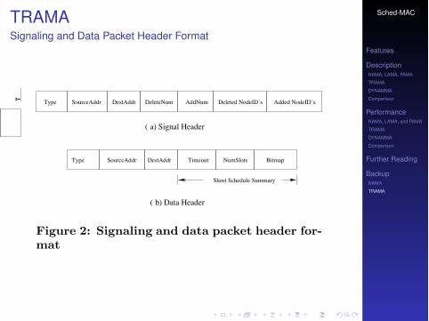
Sched-MAC
Features
DescriptionNAMA, LAMA, PAMA
TRAMA
DYNAMMA
Comparison
PerformanceNAMA, LAMA, and PAMA
TRAMA
DYNAMMA
Comparison
Further Reading
BackupNAMA
TRAMA
TRAMASignaling and Data Packet Header Format
Scheduled Access Random Access
Switching Period
Signaling Slots
Transmission Slots
Figure 1: Time slot organization
Short Schedule Summary
SourceAddr DestAddr Timeout BitmapType NumSlots
b) Data Header
Type SourceAddr DestAddr DeleteNum AddNum Deleted NodeID’s Added NodeID’s
a) Signal Header
(
(
Figure 2: Signaling and data packet header for-mat
information to select the transmitters and receivers for thecurrent time slot, leaving all other nodes in liberty to switchto low-power mode.
TRAMA assumes a single, time-slotted channel for bothdata and signaling transmissions. Figure 1 shows the overalltime-slot organization of the protocol. Time is organized assections of random- and scheduled-access periods. We re-fer to random-access slots as signaling slots and scheduled-access slots as transmission slots. Because the data ratesof a sensor network are relatively low, the duration of timeslots is much larger than typical clock drifts. For exam-ple, for a 115.2 Kbps radio, we use a transmission slot ofapproximately 46ms to transmit 512-byte application layerdata units. Hence, clock drifts in the order of ms can be tol-erated, and yet typically clock drifts are in the order of mi-croseconds or even less. This allows very simple timestampmechanisms (e.g., [10]) to be used for node synchronization.When much smaller clock drifts must be assumed and moreexpensive nodes can be used, nodes can be time synchro-nized using techniques such as GPS [9]. Accordingly, in theremainder of our description of TRAMA, we simply assumethat adequate synchronization is attained.
NP propagates one-hop neighbor information among neigh-boring nodes during the random access period using thesignaling slots, to obtain consistent two-hop topology in-formation across all nodes. As the name suggests, duringthe random access period, nodes perform contention-basedchannel acquisition and thus signaling packets are proneto collisions.
Transmission slots are used for collision-free data exchangeand also for schedule propagation. Nodes use SEP to ex-change tra!c-based information, or schedules, with neigh-bors. Essentially, schedules contain current information ontra!c coming from a node, i.e., the set of receivers for thetra!c originating at the node. A node has to announceits schedule using SEP before starting actual transmissions.SEP maintains consistent schedule information across neigh-bors and updates the schedules periodically.
AEA selects transmitters and receivers to achieve collision-free transmission using the information obtained from NPand SEP. This is the case, because electing both the trans-mitter and the receiver(s) for a particular time slot is a ne-cessity to achieve energy e!ciency in a collision-free trans-mission schedule. Random transmitter selection leads to col-lisions, and electing the transmitters and not the receiversfor a given time slot leads to energy waste, because all theneighbors around a selected transmitter have to listen in theslot, even if they are not to receive any data. Furthermore,selecting a transmitter without regard to its tra!c leads
to low channel utilization, because the selected transmit-ter may not have any data to send to the selected receiver.Hence, AEA uses tra!c information (i.e., which sender hastra!c for which receivers) to improve channel utilization.
The length of a transmission slot is fixed based on thechannel bandwidth and data size. Signaling packets are usu-ally smaller than data packets and thus transmission slotsare typically set as a multiple of signaling slots to allow foreasy synchronization. In our implementation, transmissionslots are seven times longer than signaling slots.
2.2 Access Modes and the Neighbor ProtocolIn sensor networks, nodes may fail (e.g., power drained) or
new nodes may be added (e.g., additional sensors deployed).To accommodate topology dynamics, TRAMA alternatesbetween random- and scheduled access.
TRAMA starts in random access mode where each nodetransmits by selecting a slot randomly. Nodes can only jointhe network during random access periods. The duty cycleof random- versus scheduled access depends on the type ofnetwork. In more dynamic networks, random access periodsshould occur more often. In more static scenarios, the inter-val between random access periods could be larger, becausetopology changes need to be accommodated only occasion-ally. In the case of sensor networks, there is very little or nomobility, depending on the type of application. Hence, themain function of random access periods is to permit node ad-ditions and deletions. Time synchronization could be doneduring this period. During random access periods, all nodesmust be in either transmit or receive state, so they can sendout their neighborhood updates and receive updates fromneighbors. Hence, the duration of the random access periodplays a significant role in energy consumption.
During random access periods, signaling packets may belost due to collisions, which can lead to inconsistent neigh-borhood information across nodes. To guarantee consistentneighborhood information with some degree of confidence,the length of the random access period and the number ofretransmissions of signaling packets are set accordingly. In[4], it is shown that, for a network with an average of Ntwo-hop neighbors, the number of signaling packet retrans-missions should be 7 and the retransmission interval 1.44!Nto guarantee packet delivery of 99%. Thus, the length of therandom access period will then be 7 ! 1.44 ! N .
NP gathers neighborhood information by exchanging smallsignaling packets during the random access period. Fig-ure 2(a) shows the format of the header of a signaling packet.Signaling packets carry incremental neighborhood updatesand if there are no updates, signaling packets are sent as

Sched-MAC
Features
DescriptionNAMA, LAMA, PAMA
TRAMA
DYNAMMA
Comparison
PerformanceNAMA, LAMA, and PAMA
TRAMA
DYNAMMA
Comparison
Further Reading
BackupNAMA
TRAMA
TRAMASchedule packet format
0 0 00 1 1 1 10 00 1 0 0 001 0 1 0
Reserved for particular set
of receivers depending on the
node traffic.
Does not have data, these slots could
be used by other one!hop neighbors
with data.
Reserved for
announcing the
schedule.
SourceAddr Timeout Width
32 8 8
Bitmap (Width = 4)
RESERVED GIVEUP
ChangeOver Slot
Bitmaps ....... .....
8 Width x Size
NumSlots
Field Size (bits)
Field
Figure 3: Schedule packet format
A
B C
200
79
95
100
D
Node B: Will see D as the absolute transmitter (if it decides to SLEEP then TX to SLEEP can happen)
Node A: Will be transmitting since it has the highest two!hop priority
Figure 4: Inconsistency problem
which is the last slot in the current schedule interval thatwill be used by node tx for transmission, it may assumethat the node tx is transmitting the data corresponding tothe ChangeOver slot and update the corresponding sched-ule. From now on until the schedule announced by nodetx expires, node u considers that node tx gives up winningslots for re-use. This can lead to collisions if node u tries toreuse the winning slot of node tx that is actually used fortransmission. Hence, schedules among neighbors could beunsynchronized only until the ChangeOver slot and a nodehas to listen during the ChangeOver slot of the transmitter.
It is possible for a node to get some extra slots for trans-missions in addition to the original winning slots computedwhile announcing the schedule. To prevent inconsistenciesand collisions when transmitting the schedule packet, a nodeshould always send the schedule packet only on the previ-ously announced timeout. Because all the slots after theChangeover slot are assumed as give-up slots by the neigh-bors, the schedules might be unsynchronized. Hence, trans-mitting a schedule before the timeout can potentially causecollisions with neighbors. In the following section, we de-scribe how these schedule information is used to adaptivelydecide the node state.
2.4 Adaptive Election AlgorithmIn the original NCR algorithm [5], a node is selected to
transmit if it has the highest priority among its contendingset. Node u’s contending set is the set of all nodes that arein u’s two-hop neighborhood. Node u’s priority at time slott is defined as the pseudo-random hash of the concatenationof node u’s identity and t, or
prio(u, t) = hash(u! t) (1)
Assuming that node identities are unique and nodes aresynchronized, all nodes compute the same priority value atany given time slot. However, if the selected node does nothave any data to send, then the slot is wasted. Furthermore,nodes are free to transmit to any one-hop neighbor, becausethere is no sleep state in NCR.
For energy e!ciency, TRAMA switches nodes to sleepstate whenever possible, and attempts to re-use slots thatare not used by the selected transmitter for bandwidth ef-ficiency. A selected node may give up its transmission slot
if it does not have any packets to send; this slot could thenbe used by another node. Nodes exchange current tra!cinformation with their neighbors to make e"ective use oflow-power, idle radio mode and accomplish slot re-use.
At any given time slot t during the scheduled access pe-riod, the state of a given node u is determined based onu’s two-hop neighborhood information and the schedulesannounced by u’s one-hop neighbors. Possible states are:transmit (TX), receive (RX), and sleep (SL).
At any given slot t, a node u is in the TX state if: (1) uhas the highest priority, i.e., prio(u, t) among its contendingset and (2) u has data to send.
A node is in the RX state when it is the intended re-ceiver of the current transmitter. Otherwise, the node canbe switched o" to the SL state, because it is not participat-ing in any data exchange. This means that, if a node is notthe selected transmitter, it will decide whether it needs tobe in RX state by consulting the schedule sent out by theselected transmitter. If the transmitter does not have tra!cdestined for that node in the current slot, the node can thensleep.
Each node executes AEA to decide its current state ( TX,RX, or SL) based on current node priorities (within itstwo-hop neighborhood) and also on the announced schedulesfrom one-hop neighbors. The algorithm’s pseudo-code isprovided in Figure 5. Table 1 lists some basic terminologyand notation used in the description of AEA.
The state of a node depends on the Absolute Winner andthe announced schedules from its one-hop neighbors. Fromnode u’s point of view, the Absolute Winner at any giventime slot t can be: (1) node u itself, (2) node v that liesin the two-hop neighborhood of node u in which case theAlternate Winner atx(u) needs to be accounted for if hiddenfrom node v, or (3) a node w that lies in node u’s one-hopneighborhood.
Whenever a node becomes an Absolute Winner for a par-ticular timeslot and has announced a non-zero bitmap forthis slot, it knows that no other node in its two-hop neigh-borhood will be transmitting in this slot. Thus, the nodecan transmit collision-free to its intended receiver(s). Whena node is not an Absolute Winner, it is not certain who theactual transmitter for a particular slot is. For example, con-sider the topology shown in Figure 4. Let D be the node