Scatter Plots Using PROC SGPLOT for that Thursday...

SESUG 2011

1

Paper PO-04

Scatter Plots Using PROC SGPLOT for that Thursday Presentation

Sharon Matsumoto Hirabayashi

ABSTRACT

It always starts with “I have a simple request.”

This time, it was a request for a scatter plot of two variables by a third variable in a listing.

The PROC PLOT was nice, but could we overlay the plots instead of having a separate plot for each by-group? Could we label the points in the plot with the by-group values? Could we group the points using the categories of another variable, using different colors and symbols to distinguish the groups? Could we add a 45-degree reference line? Could we do this for twelve other plots, maintaining the same legend across all thirteen plots? And, since the presentation is on Thursday, can we have the plots ready by Tuesday?

Egads. Thank goodness for SAS® online documentation, and that our company had migrated to SAS v9.2! This paper details how SAS ODS Graphics, PROC SGPLOT, and the %MODSTYLE macro were used to quickly and painlessly generate not just nice graphics, but really nice graphics for that Thursday presentation.

INTRODUCTION As SAS programmers, we all know that what starts out as a simple request can mushroom into something quite stress-provoking, especially when a vague deadline suddenly turns ominous, and you find yourself working in an area just beyond your comfort zone. That’s when you truly appreciate SAS online documentation. I know I did when I was tasked with producing the scatter plots described above. I also appreciated that our company had installed SAS v9.2 with SAS/GRAPH®, because that made PROC SGPLOT available. After quickly scanning through the SAS documentation, I decided early on that SGPLOT offered less cumbersome coding options and would get me as far as I needed (or was willing) to go. This paper will describe some of that coding and will hopefully offer some tips for a SAS programmer charged with a similar “simple” request.

INPUT DATA

For this paper, the source of the data is not as important as simply having data to plot, so to make things easier to illustrate, I changed both the content and scope from the original work by using a different input data set. Here, the source of data originates from test scores downloaded from a county website. I created a SAS data set (mydata) from those scores, with one record per school/test subject, each record containing an identifier for school (my_datapoint_var), test subject (my_by_var), test scores by gender (my_x_var, my_y_var), and a four-level categorical variable indicating how the percentage of students by gender taking the test compared to the overall county percentage (my_group_var). I further edited the data set to demonstrate legend differences.

DESCRIPTION OF PLOTS

In all of the graphs described below, for each value of my_datapoint_var, points were plotted using values of my_x_var for the x-axis, and values of my_y_var for the y-axis. Separate plots were generated for each value of my_by_var.

The programs to generate the plots were run on a PC in batch mode under SAS v9.2 with Base SAS and SAS/GRAPH.

I will describe how I coded SGPLOT, starting with a simple scatter plot, and the steps I took to modify it, based on subsequent requests.

Specifically, I will show how to:

1. Produce a simple scatter plot

2. Label the axes

3. Label the data points

4. Group the data points using colors and symbols

SESUG 2011

2

5. Use the %MODSTYLE macro to set non-default colors and symbols

6. Maintain the same colors and symbols across plots

7. Add a 45-degree line

8. Change the color of the 45-degree line

9. Label the legend for the colors and symbols

10. Position the legend

11. Adjust the height and width of the plot

12. Specify the output location

A SIMPLE SCATTER PLOT WITH SGPLOT

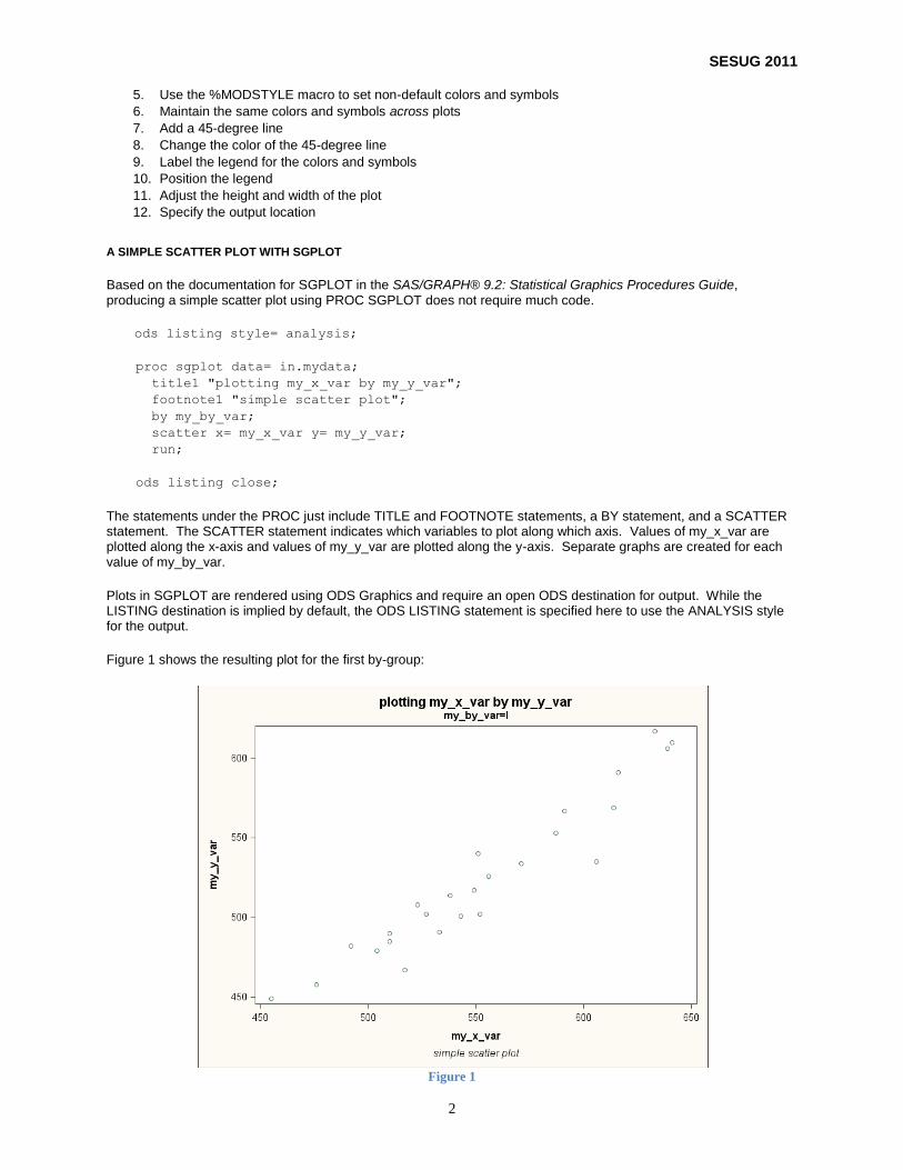
Based on the documentation for SGPLOT in the SAS/GRAPH® 9.2: Statistical Graphics Procedures Guide, producing a simple scatter plot using PROC SGPLOT does not require much code.

ods listing style= analysis;

proc sgplot data= in.mydata;

title1 "plotting my_x_var by my_y_var";

footnote1 "simple scatter plot";

by my_by_var;

scatter x= my_x_var y= my_y_var;

run;

ods listing close;

The statements under the PROC just include TITLE and FOOTNOTE statements, a BY statement, and a SCATTER statement. The SCATTER statement indicates which variables to plot along which axis. Values of my_x_var are plotted along the x-axis and values of my_y_var are plotted along the y-axis. Separate graphs are created for each value of my_by_var.

Plots in SGPLOT are rendered using ODS Graphics and require an open ODS destination for output. While the LISTING destination is implied by default, the ODS LISTING statement is specified here to use the ANALYSIS style for the output.

Figure 1 shows the resulting plot for the first by-group:

Figure 1

SESUG 2011

3

Note that SGPLOT produces graphics output, and no LST file is generated. Instead, PNG image files are created, one file for each by-group value. By default, the image files are named with the procedure name, an index to differentiate the by-group plots, and the image type extension (SGPlot.png, SGPlot1.png, and SGPlot2.png).

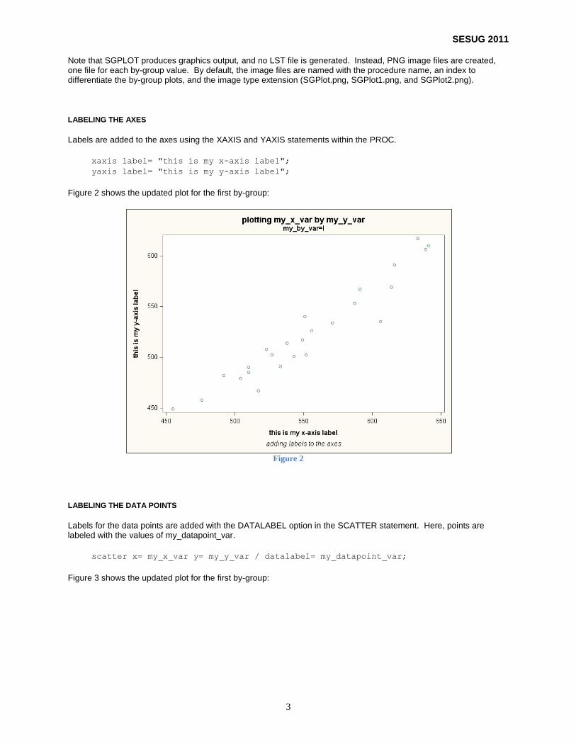
LABELING THE AXES

Labels are added to the axes using the XAXIS and YAXIS statements within the PROC.

xaxis label= "this is my x-axis label";

yaxis label= "this is my y-axis label";

Figure 2 shows the updated plot for the first by-group:

Figure 2

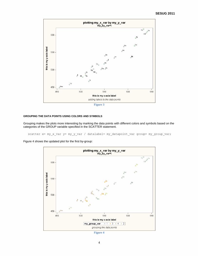
LABELING THE DATA POINTS

Labels for the data points are added with the DATALABEL option in the SCATTER statement. Here, points are labeled with the values of my_datapoint_var.

scatter x= my_x_var y= my_y_var / datalabel= my_datapoint_var;


SESUG 2011

4

Figure 3

GROUPING THE DATA POINTS USING COLORS AND SYMBOLS

Grouping makes the plots more interesting by marking the data points with different colors and symbols based on the categories of the GROUP variable specified in the SCATTER statement.

scatter x= my_x_var y= my_y_var / datalabel= my_datapoint_var group= my_group_var;


Figure 4

SESUG 2011

5

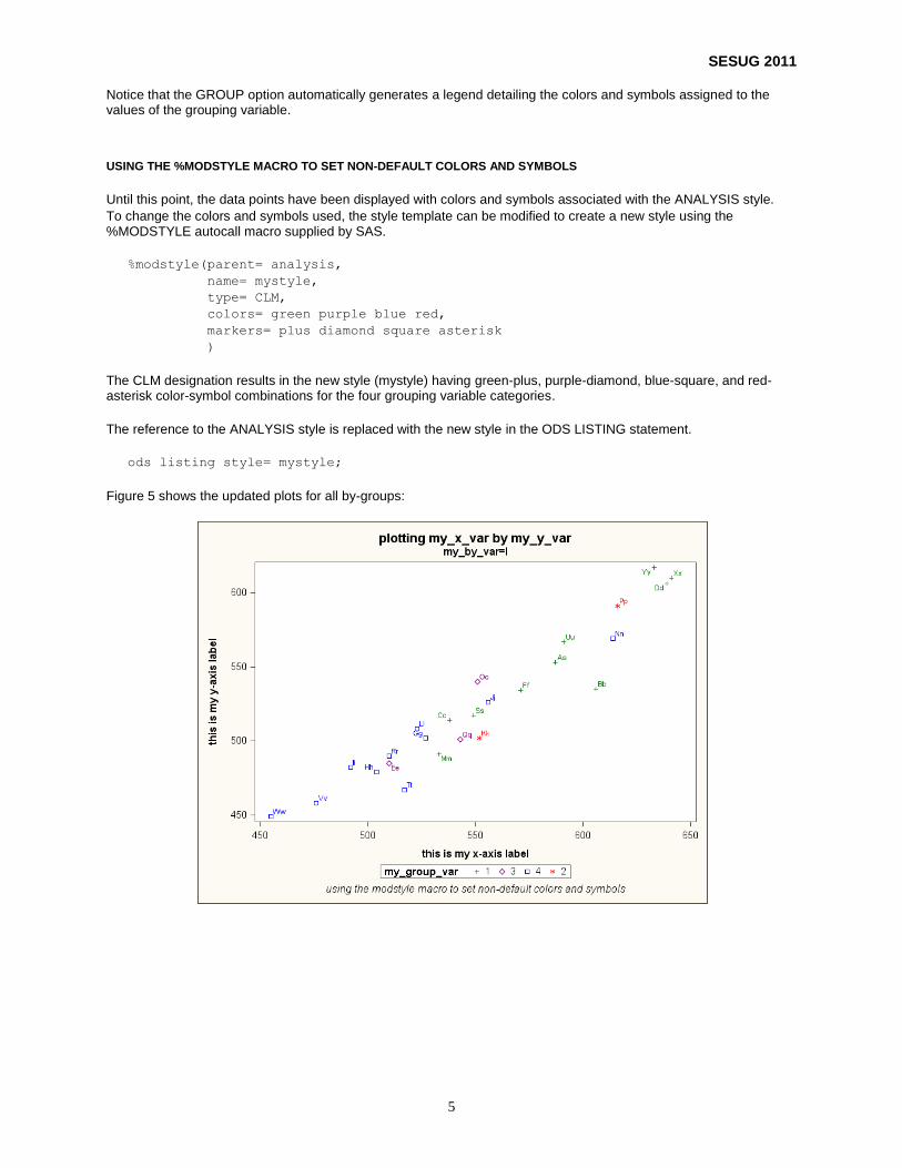
Notice that the GROUP option automatically generates a legend detailing the colors and symbols assigned to the values of the grouping variable.

USING THE %MODSTYLE MACRO TO SET NON-DEFAULT COLORS AND SYMBOLS

Until this point, the data points have been displayed with colors and symbols associated with the ANALYSIS style.

To change the colors and symbols used, the style template can be modified to create a new style using the %MODSTYLE autocall macro supplied by SAS.

%modstyle(parent= analysis,

name= mystyle,

type= CLM,

colors= green purple blue red,

markers= plus diamond square asterisk

)

The CLM designation results in the new style (mystyle) having green-plus, purple-diamond, blue-square, and red-asterisk color-symbol combinations for the four grouping variable categories.

The reference to the ANALYSIS style is replaced with the new style in the ODS LISTING statement.

ods listing style= mystyle;

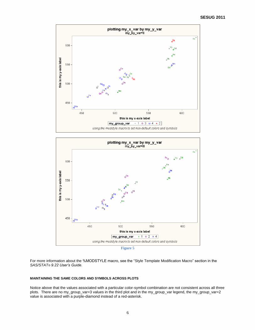
Figure 5 shows the updated plots for all by-groups:

SESUG 2011

6

Figure 5

For more information about the %MODSTYLE macro, see the “Style Template Modification Macro” section in the SAS/STAT® 9.22 User’s Guide.

MAINTAINING THE SAME COLORS AND SYMBOLS ACROSS PLOTS

Notice above that the values associated with a particular color-symbol combination are not consistent across all three plots. There are no my_group_var=3 values in the third plot and in the my_group_var legend, the my_group_var=2 value is associated with a purple-diamond instead of a red-asterisk.

SESUG 2011

7

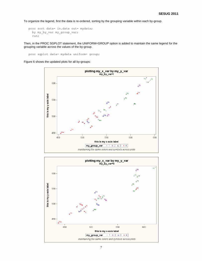
To organize the legend, first the data is re-ordered, sorting by the grouping variable within each by-group.

proc sort data= in.data out= mydata;

by my_by_var my_group_var;

run;

Then, in the PROC SGPLOT statement, the UNIFORM=GROUP option is added to maintain the same legend for the grouping variable across the values of the by-group.

proc sgplot data= mydata uniform= group;

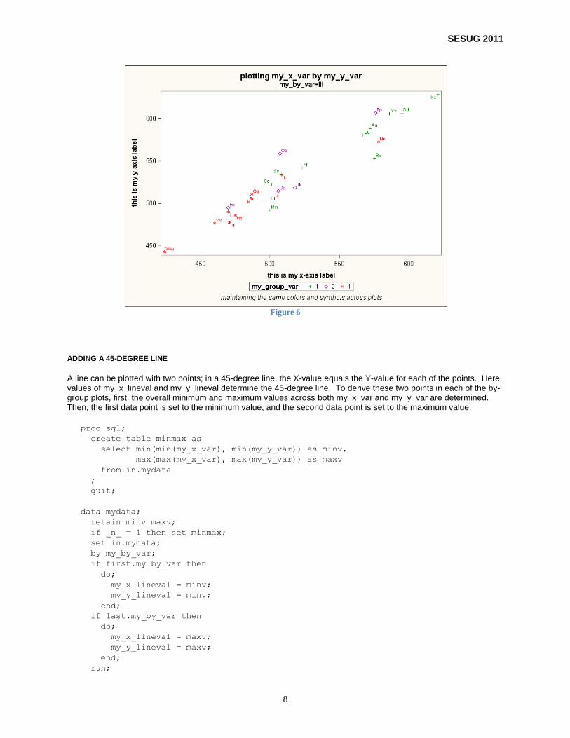
Figure 6 shows the updated plots for all by-groups:

SESUG 2011

8

Figure 6

ADDING A 45-DEGREE LINE

A line can be plotted with two points; in a 45-degree line, the X-value equals the Y-value for each of the points. Here, values of my_x_lineval and my_y_lineval determine the 45-degree line. To derive these two points in each of the by-group plots, first, the overall minimum and maximum values across both my_x_var and my_y_var are determined. Then, the first data point is set to the minimum value, and the second data point is set to the maximum value.

proc sql;

create table minmax as

select min(min(my_x_var), min(my_y_var)) as minv,

max(max(my_x_var), max(my_y_var)) as maxv

from in.mydata

;

quit;

data mydata;

retain minv maxv;

if _n_ = 1 then set minmax;

set in.mydata;

by my_by_var;

if first.my_by_var then

do;

my_x_lineval = minv;

my_y_lineval = minv;

end;

if last.my_by_var then

do;

my_x_lineval = maxv;

my_y_lineval = maxv;

end;

run;

SESUG 2011

9

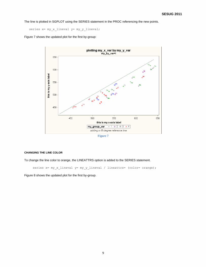
The line is plotted in SGPLOT using the SERIES statement in the PROC referencing the new points.

series x= my_x_lineval y= my_y_lineval;


Figure 7

CHANGING THE LINE COLOR

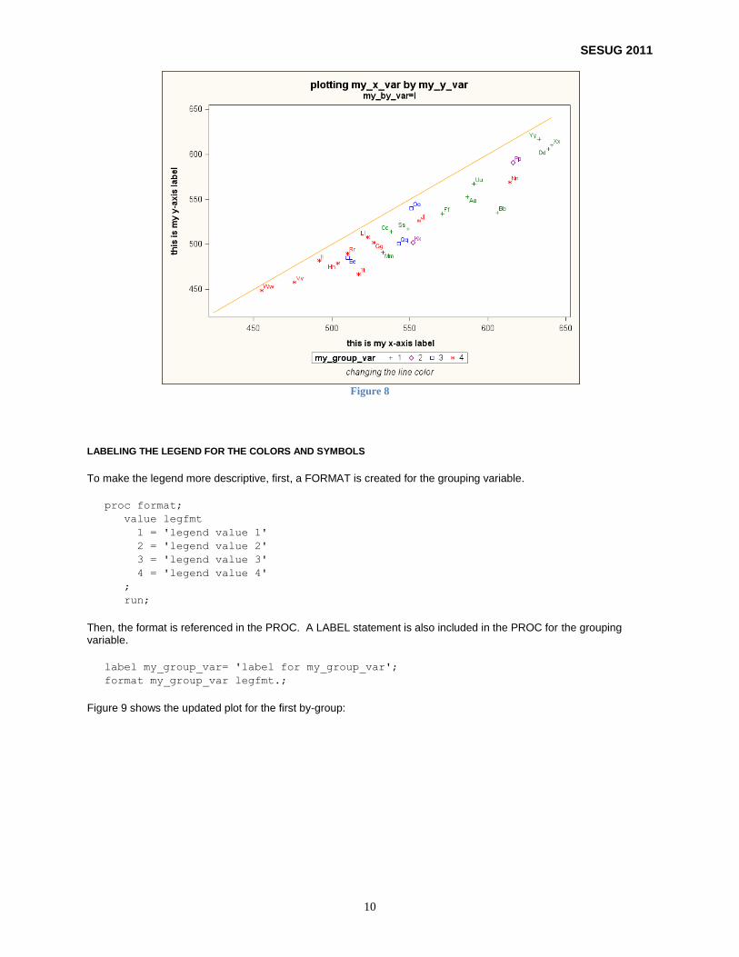
To change the line color to orange, the LINEATTRS option is added to the SERIES statement.

series x= my_x_lineval y= my_y_lineval / lineattrs= (color= orange);

Figure 8 shows the updated plot for the first by-group.

SESUG 2011

10

Figure 8

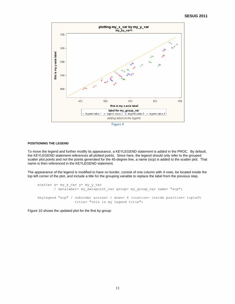
LABELING THE LEGEND FOR THE COLORS AND SYMBOLS

To make the legend more descriptive, first, a FORMAT is created for the grouping variable.

proc format;

value legfmt

1 = 'legend value 1'




;

run;

Then, the format is referenced in the PROC. A LABEL statement is also included in the PROC for the grouping variable.

label my_group_var= 'label for my_group_var';

format my_group_var legfmt.;


SESUG 2011

11

Figure 9

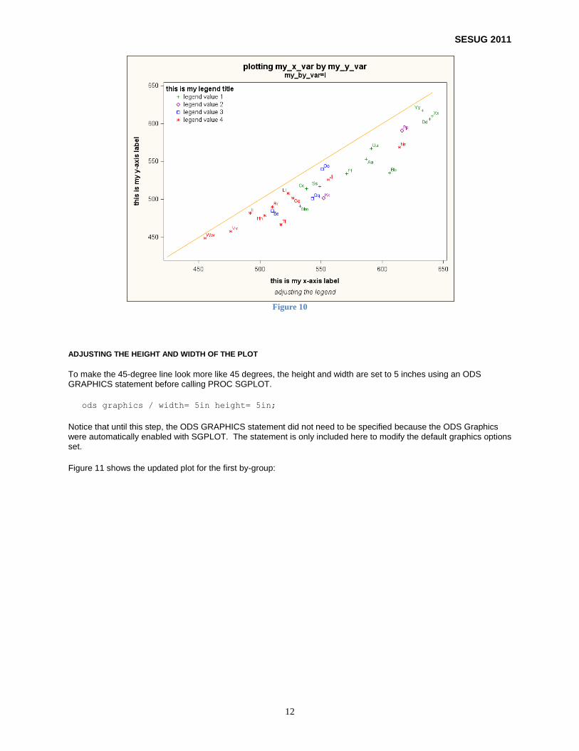
POSITIONING THE LEGEND

To move the legend and further modify its appearance, a KEYLEGEND statement is added in the PROC. By default, the KEYLEGEND statement references all plotted points. Since here, the legend should only refer to the grouped scatter plot points and not the points generated for the 45-degree line, a name (scp) is added to the scatter plot. That name is then referenced in the KEYLEGEND statement.

The appearance of the legend is modified to have no border, consist of one column with 4 rows, be located inside the top left corner of the plot, and include a title for the grouping variable to replace the label from the previous step.

scatter x= my_x_var y= my_y_var

/ datalabel= my_datapoint_var group= my_group_var name= "scp";

keylegend "scp" / noborder across= 1 down= 4 location= inside position= topleft

title= "this is my legend title";


SESUG 2011

12

Figure 10

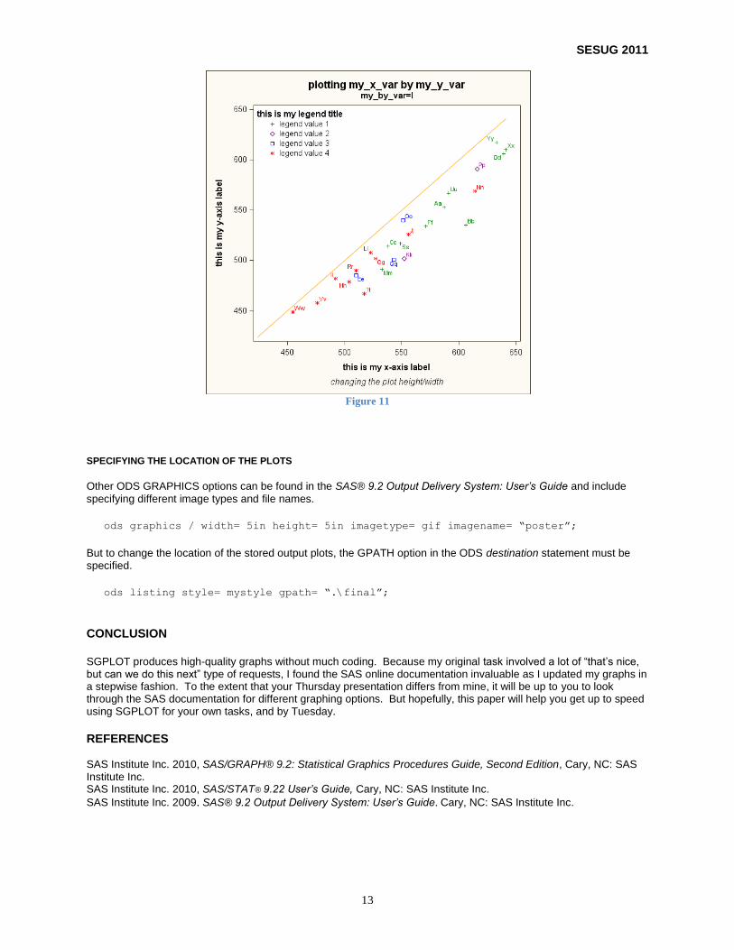
ADJUSTING THE HEIGHT AND WIDTH OF THE PLOT

To make the 45-degree line look more like 45 degrees, the height and width are set to 5 inches using an ODS GRAPHICS statement before calling PROC SGPLOT.

ods graphics / width= 5in height= 5in;

Notice that until this step, the ODS GRAPHICS statement did not need to be specified because the ODS Graphics were automatically enabled with SGPLOT. The statement is only included here to modify the default graphics options set.


SESUG 2011

13

Figure 11

SPECIFYING THE LOCATION OF THE PLOTS

Other ODS GRAPHICS options can be found in the SAS® 9.2 Output Delivery System: User’s Guide and include

specifying different image types and file names.

ods graphics / width= 5in height= 5in imagetype= gif imagename= “poster”;

But to change the location of the stored output plots, the GPATH option in the ODS destination statement must be specified.

ods listing style= mystyle gpath= “.\final”;

CONCLUSION

SGPLOT produces high-quality graphs without much coding. Because my original task involved a lot of “that’s nice, but can we do this next” type of requests, I found the SAS online documentation invaluable as I updated my graphs in a stepwise fashion. To the extent that your Thursday presentation differs from mine, it will be up to you to look through the SAS documentation for different graphing options. But hopefully, this paper will help you get up to speed using SGPLOT for your own tasks, and by Tuesday.

REFERENCES SAS Institute Inc. 2010, SAS/GRAPH® 9.2: Statistical Graphics Procedures Guide, Second Edition, Cary, NC: SAS Institute Inc. SAS Institute Inc. 2010, SAS/STAT® 9.22 User’s Guide, Cary, NC: SAS Institute Inc.

SAS Institute Inc. 2009. SAS® 9.2 Output Delivery System: User’s Guide. Cary, NC: SAS Institute Inc.

SESUG 2011

14

ACKNOWLEDGMENTS

The author wishes to thank the following folks at Westat: Mike Rhoads for his review, and John Burke for his support and for always reminding me that necessity is the mother of invention.

CONTACT INFORMATION

Comments and questions are welcomed by the author:

Sharon Hirabayashi

E-mail: [email protected]

This presentation was developed while the author was employed at Westat, but the contents of this paper are the work of the author and do not necessarily represent the opinions, recommendations, or practices of Westat.

SAS and all other SAS Institute Inc. product or service names are registered trademarks or trademarks of SAS Institute Inc. in the USA and other countries. ® indicates USA registration.

Other brand and product names are trademarks of their respective companies.

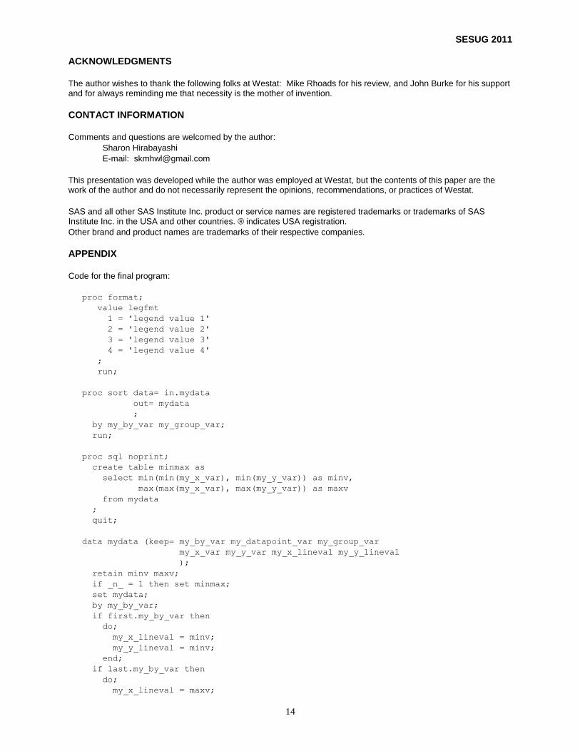
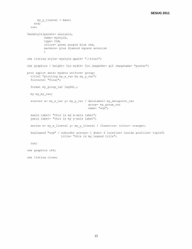
APPENDIX

Code for the final program:

proc format;

value legfmt





;

run;

proc sort data= in.mydata

out= mydata

;

by my_by_var my_group_var;

run;

proc sql noprint;

create table minmax as

select min(min(my_x_var), min(my_y_var)) as minv,

max(max(my_x_var), max(my_y_var)) as maxv

from mydata

;

quit;

data mydata (keep= my_by_var my_datapoint_var my_group_var

my_x_var my_y_var my_x_lineval my_y_lineval

);

retain minv maxv;

if _n_ = 1 then set minmax;

set mydata;

by my_by_var;

if first.my_by_var then

do;

my_x_lineval = minv;

my_y_lineval = minv;

end;

if last.my_by_var then

do;

my_x_lineval = maxv;

SESUG 2011

15

my_y_lineval = maxv;

end;

run;

%modstyle(parent= analysis,

name= mystyle,

type= CLM,

colors= green purple blue red,

markers= plus diamond square asterisk

)

ods listing style= mystyle gpath= ".\final";

ods graphics / height= 5in width= 5in imagefmt= gif imagename= "poster";

proc sgplot data= mydata uniform= group;

title1 "plotting my_x_var by my_y_var";

footnote1 "final";

format my_group_var legfmt.;

by my_by_var;

scatter x= my_x_var y= my_y_var / datalabel= my_datapoint_var

group= my_group_var

name= "scp";

xaxis label= "this is my x-axis label";

yaxis label= "this is my y-axis label";

series x= my_x_lineval y= my_y_lineval / lineattrs= (color= orange);

keylegend "scp" / noborder across= 1 down= 4 location= inside position= topleft

title= "this is my legend title";

run;

ods graphics off;

ods listing close;

Scatter Plots Using PROC SGPLOT for that Thursday...

Documents

Transcript of Scatter Plots Using PROC SGPLOT for that Thursday...