Scanning: CSE 337: Introduction to Medical Imaging Lecture ...

CSE 337: Introduction to Medical Imaging

Lecture 6: X-Ray Computed Tomography

Klaus Mueller

Computer Science Department

Stony Brook University

Overview

Scanning:rotate source-detector pair around the patient

sinogram: a line for every angle

reconstruction routine

reconstructed cross-sectional slice

data

Early Beginnings

Linear tomographyonly line P1-P2 stays in focusall others appear blurred

Axial tomographyin principle, simulates the backprojection procedure used in current times

film

Current Technology

Principles derived by Godfrey Hounsfield for EMI

• based on mathematics by A. Cormack

• both received the Nobel Price in medizine/physiology in 1979

• technology is advanced to this day

Images:

• size generally 512 x 512 pixels

• values in Hounsfield units (HU) in the range of –1000 to 1000

µ: linear attenuation coefficient

• due to large dynamic range, windowing must be used to view an image

CT Detectors

Scintillation crystal with photomultiplier tube (PMT)

(scintillator: material that converts ionizing radiation into pulses of light)

• high QE and response time

• low packing density

• PMT used only in the early CT scanners

Gas ionization chambers

• replace PMT

• X-rays cause ionization of gas molecules in chamber

• ionization results in free electrons/ions

• these drift to anode/cathode and yield a measurable electric signal

• lower QE and response time than PMT systems, but higher packing density

Scintillation crystals with photodiode

• current technology (based on solid state or semiconductors)

• photodiodes convert scintillations into measurable electric current

• QE > 98% and very fast response time

Projection Coordinate System

The parallel-beam geometry at angle θ represents a new coordinate system (r,s) in which projection Iθ(r) is acquired• rotation matrix R transforms coordinate system (x, y) to (r, s):

that is, all (x,y) points that fulfill r = x cos(θ ) + y sin(θ)

are on the (ray) line L(r,θ)

• RT is the inverse, mapping (r, s) to (x, y)

s is the parametric variable along the (ray) line L(r,θ)

cos sin

sin cos

r x xR

s y y

θ θ

θ θ

= =

−

cos sin

sin cos

Tx r r

Ry s s

θ θ

θ θ

− = =

Projection

Assuming a fixed angle θ, the measured intensity at detector position r is the integrated density along L(r,θ):

For a continuous energy spectrum:

But in practice, is is assumed that the X-rays are monochromatic

,

,

( , )

0

( cos sin , sin cos )

0

( )Lr

Lr

x y ds

r s r s ds

I r I e

I e

θ

θ

µ

θ

µ θ θ θ θ

−

⋅ − ⋅ ⋅ + ⋅

∫= ⋅

∫= ⋅

,


0

0

( ) ( )Lr

r s r s ds

I r I E e θ

µ θ θ θ θ

θ

⋅ − ⋅ ⋅ + ⋅∞ ∫= ⋅∫

Projection Profile

Each intensity profile Iθ(r) is transformed into an attenuation profile pθ(r):

• pθ(r) is zero for |r|>FOV/2 (FOV = Field of View, detector width)

• pθ(r) can be measured from (0, 2π)

• however, for parallel beam views (π, 2π) are redundant, so just need to measure from (0, π)

,0

( )( ) ln ( cos sin , sin cos )

rL

I rp r r s r s ds

Iθ

θθ µ θ θ θ θ= − = ⋅ − ⋅ ⋅ + ⋅∫

Iθ(r) pθ(r)

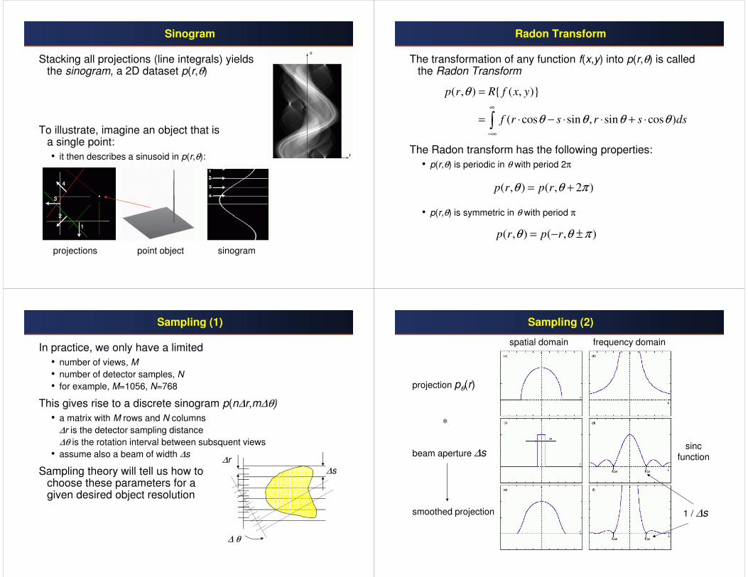
Sinogram

Stacking all projections (line integrals) yields the sinogram, a 2D dataset p(r,θ)

To illustrate, imagine an object that is a single point:

• it then describes a sinusoid in p(r,θ):

projections point object sinogram

Radon Transform

The transformation of any function f(x,y) into p(r,θ) is called the Radon Transform

The Radon transform has the following properties:

• p(r,θ) is periodic in θ with period 2π

• p(r,θ) is symmetric in θ with period π

( , ) { ( , )}


p r R f x y

f r s r s ds

θ

θ θ θ θ∞

−∞

=

= ⋅ − ⋅ ⋅ + ⋅∫

( , ) ( , 2 )p r p rθ θ π= +

( , ) ( , )p r p rθ θ π= − ±

Sampling (1)

In practice, we only have a limited

• number of views, M

• number of detector samples, N

• for example, M=1056, N=768

This gives rise to a discrete sinogram p(n∆r,m∆θ)

• a matrix with M rows and N columns

∆r is the detector sampling distance

∆θ is the rotation interval between subsquent views

• assume also a beam of width ∆s

Sampling theory will tell us how to choose these parameters for a given desired object resolution

∆r∆s

∆ θ

Sampling (2)

projection pθ(r)

spatial domain frequency domain

beam aperture ∆s

smoothed projection

*

1 / ∆s

sinc function

Sampling (3)

sampling at ∆r

spatial domain frequency domain

sampled projection

smoothed projection

1 / ∆r

.

1 / ∆s

Limiting Aliasing

Aliasing within the sinogram lines (projection aliasing):

• to limit aliasing, we must separate the aliases in the frequency domain (at least coinciding the zero-crossings):

• thus, at least 2 samples per beam are required

Aliasing across the sinogram lines (angular aliasing):

1 2

2

sr

r s

∆≥ → ∆ ≤

∆ ∆

∆θ

max

max

max max

/ 2

for uniform sampling: / 2 2

k

M

kk

N

k k Nk M

M N

πθ

πθ π

∆ =

∆ =

∆ = ∆ → = → =

sinogram in the frequency

domain

(2 projections with N=12

samples each are shown)

∆k

kmax=1/∆r

M: number of views, evenly distributed around the semi-circle

N: number of detector samples,

give rise to N frequency domain

samples for each projection

Reconstruction: Concept

Given the sinogram p(r,θ) we want to recover the object described in (x,y) coordinates

Recall the early axial tomography method

• basically it worked by subsequently “smearing” the acquired p(r,θ) across a film plate

• for a simple point we would get:

This is called backprojection:

0

( , ) { ( , )} ( cos sin , )b x y B p r p x y d

π

θ θ θ θ θ= = ⋅ + ⋅∫

Backprojection: Illustration

Backprojection: Practical Considerations

A few issues remain for practical use of this theory:

• we only have a finite set of M projections and a discrete array of Npixels (xi, yj)

• to reconstruct a pixel (xi, yj) there may not be a ray p(rn,θn) (detector sample) in the projection set

� this requires interpolation (usually linear interpolation is used)

• the reconstructions obtained with the simple backprojection appear blurred (see previous slides)

1

( , ) { ( , )} ( cos sin , )M

i j n m i m j m m

m

b x y B p r p x yθ θ θ θ=

= = ⋅ + ⋅∑

interpolation

detector samples

pixelray

To understand the blurring we need more theory � the Fourier Slice Theorem or Central Slice Theorem

• it states that the Fourier transform P(θ,k) of a projection p(r,θ) is a line across the origin of the Fourier transform F(kx,ky) of function f(x,y)

A possible reconstruction procedure would then:

• calculate the 1D FT of all projections p(rm,θm), which gives rise to F(kx,ky) sampled on a polar grid (see figure)

• resample the polar grid into a cartesian grid (using interpolation)

• perform inverse 2D FT to obtain the desired f(x,y) on a cartesian grid

However, there are two important observations:

• interpolation in the frequency domain leads to artifacts

• at the FT periphery the spectrum is only sparsely sampled

The Fourier Slice Theorem

polar grid

Filtered Backprojection: Concept

To account for the implications of these two observations, we modify the reconstruction procedure as follows:

• filter the projections to compensate for the blurring

• perform the interpolation in the spatial domain via backprojection

� hence the name Filtered Backprojection

Filtering -- what follows is a more practical explanation (for formal proof see the book):

• we need a way to equalize the contributions of all frequencies in the FT’s polar grid

• this can be done by multiplying each P(θ,k) by a ramp function � this way the magnitudes of the existing higher-frequency samples in each projection are scaled up to compensate for their lower amount

• the ramp is the appropriate scaling function since the sample density decreases linearly towards the FT’s periphery

ramp

Filtered Backprojection: Equation and Result

Recall the previous (blurred) backprojection illustration

• now using the filtered projections:

2

0

( , ) ( ( , ) ) i krf x y P k k e dk d

ππθ θ

∞

−∞

= ⋅ ⋅∫ ∫

ramp-filtering

inverse 1D Fourier transform � p(r,θ)backprojection for all angles

not filtered filtered

1D Fouriertransform of p(r,θ)

� P(k,θ)

Filtered Backprojection: Illustration Filters

There are various filters (for formulas see the book) :

• all filters have large spatial extent � convolution would be expensive

• therefore the filtering is usually done in the frequency domain � the required two FT’s plus the multiplication by the filter function has lower complexity

Popular filters (for formulas see book):

• Ram-Lak: original ramp filter limited to interval [±kmax]

• Ram-Lak with Hanning/Hamming smoothing window: de-emphasizes the higher spatial frequencies to reduce aliasing and noise

Ram-Lak

Hamming window

Windowed Ram-LakHanning window

Filters (2)

Frequency domain:

• #1: Ram-Lak

• #2: Shepp-Logan

• #3: cosine

• #4: Hamming (α=0.54) and Hanning (α=0.5)

( )H k k=

spatial domain

frequency domain

max

( ) sinc( )2

kH k k

k

π= ⋅

kmax

H(k)

max( ) cos( / )H k k k=

max

( ) (1 )cos( )k

H kk

πα α= + −

Beam Geometry

The parallel-beam configuration is not practical

• it requires a new source location for each ray

We’d rather get an image in “one shot”

• the requires fan-beam acquisition

parallel-beam fan-beamcone-beam in 3D

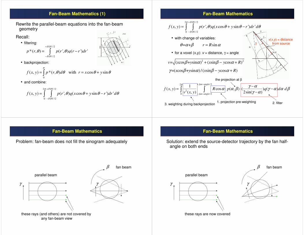
Fan-Beam Mathematics (1)

Rewrite the parallel-beam equations into the fan-beam geometry

Recall:

• filtering:

• backprojection:

• and combine:

0

( , ) *( , ) with cos sinf x y p r d r x y

π

θ θ θ θ= = +∫

/ 2

/ 2

*( , ) ( ', ) ( ') '

FOV

FOV

p r p r q r r drθ θ+

−

= −∫

2 / 2

0 / 2

( , ) ( ', ) ( cos sin ') '

FOV

FOV

f x y p r q x y r dr d

π

θ θ θ θ+

−

= + −∫ ∫

Fan-Beam Mathematics

• with change of variables:

• for a voxel (x,y): v = distance, γ = angle

2 / 2

0 / 2

( , ) ( ', ) ( cos sin ') '

FOV

FOV

f x y p r q x y r dr d

π

θ θ θ θ+

−

= + −∫ ∫

= + sin r Rθ α β α=

/ 22

2

0 / 2

1( , ) cos ( , ) ( ) ( )

( , ) 2sin( )

fan angle

fan angle

f x y R p q d dv x y

πγ α

α α β γ α α βγ α

+ −

− −

−= ⋅ ⋅ −

−∫ ∫

2. filter

the projection at β

1. projection pre-weighting3. weighting during backprojection

v(x,y) = distance

from source

2 2= ( cos + sin ) ( sin cos ) v x y x y Rβ α β α+ − +

=( cos + sin ) / ( sin cos ) x y x y Rγ β α β α− +

γ


Problem: fan-beam does not fill the sinogram adequately

β

γ

these rays (and others) are not covered by any fan-beam view

parallel beam

fan beam

γ


Solution: extend the source-detector trajectory by the fan half-angle on both ends

β

γ

these rays are now covered

parallel beam

fan beam

γ


More formally

• region A is covered twice, while region B is not covered at all


Extending the trajectory fills the space

• but some areas are filled twice, which causes problems


Simply setting these regions to zero will result in heavy streak artifacts

• recall the filtering step?

Need to use a smoother window

• a smooth window is both continuous and has a continuous derivative at the boundary of single and double-overlap regions

• the window weights for the same rays at opposite sides of the sinogram must be 1.

• the Parker window fullfills these conditions:

Fan-Beam Mathematics (3)

See chapter in Kak-Slaney (posted on the class website) for equations associated with flat detectors

Compare with parallel beam sinogram fill

β

γ

these rays (and others) are not covered by any fan-beam view

parallel beam fan beam

Remarks

In practice, need only fan-beam data in the angular range [-fan-angle/2, 180°+fan-angle/2]

So, reconstruction from fan-beam data involves• a pre-weighting of the projection data, depending on α• a pre-weighting of the filter (here we used the spatial domain filters)• a backprojection along the fan-beam rays (interpolation as usual)• a weighting of the contributions at the reconstructed pixels,

depending on their distance v(x, y) from the source

Alternatively, one could also “rebin” the data into a parallel-beam configuration• however, this requires an additional interpolation since there is no

direct mapping into a uniform paralle-bealm configuration

Lastly, there are also iterative algorithms• these pose the reconstruction problem as a system of linear

equations• solution via iterative solves (more to come in the nuclear medicine

lectures)


See chapter in Kak-Slaney (posted on the class website) for equations associated with flat detectors

Imaging in Three Dimensions

Sequential CT

• advance table with patient after each slice acquisition has been completed

• stop-motion is time consuming and also shakes the patient

• the effective thickness of a slice, ∆z, is equivalent to the beam width ∆s in 2D

• similarly: we must acquire 2 slices per ∆z to combat aliasing

Spiral (helical) CT

• table translates as tube rotates around the patient

• very popular technique

• fast and continuous

• table feed (TF) = axial translation per tube rotation

• pitch = TF / ∆z

∆z

z

Reconstruction From Spiral CT Data

Note: the table is advancing (z grows) while the tube rotates (β grows) • however,the reconstruction of a slice with constant z requires data

from all angles β• � require some form of interpolation

• if TF=∆z/2 (see before), then a good pitch=(∆z/2) / ∆z = 0.5 • since opposing rays (β=[180°…360°]) have (roughly) the same

information, TF can double (and so can pitch = 1)• in practice, pitch is typically between 1 and 2• higher pitch lowers dose, scan-time, and reduces motion artifacts

sequential CT spiral CT

available data

interpolated

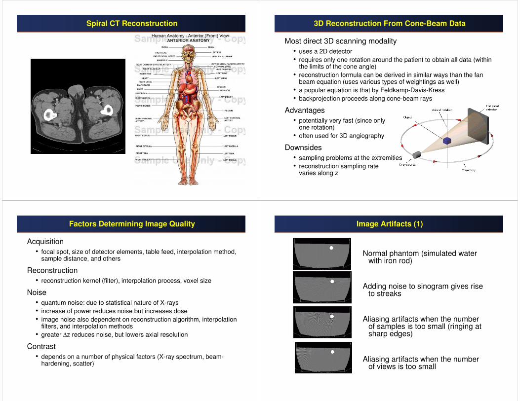
Spiral CT Reconstruction 3D Reconstruction From Cone-Beam Data

Most direct 3D scanning modality

• uses a 2D detector

• requires only one rotation around the patient to obtain all data (within the limits of the cone angle)

• reconstruction formula can be derived in similar ways than the fan beam equation (uses various types of weightings as well)

• a popular equation is that by Feldkamp-Davis-Kress

• backprojection proceeds along cone-beam rays

Advantages

• potentially very fast (since only one rotation)

• often used for 3D angiography

Downsides

• sampling problems at the extremities

• reconstruction sampling rate varies along z

Factors Determining Image Quality

Acquisition

• focal spot, size of detector elements, table feed, interpolation method, sample distance, and others

Reconstruction

• reconstruction kernel (filter), interpolation process, voxel size

Noise

• quantum noise: due to statistical nature of X-rays

• increase of power reduces noise but increases dose

• image noise also dependent on reconstruction algorithm, interpolation filters, and interpolation methods

• greater ∆z reduces noise, but lowers axial resolution

Contrast

• depends on a number of physical factors (X-ray spectrum, beam-hardening, scatter)

Image Artifacts (1)

Normal phantom (simulated water with iron rod)

Adding noise to sinogram gives rise to streaks

Aliasing artifacts when the number of samples is too small (ringing at sharp edges)

Aliasing artifacts when the number of views is too small

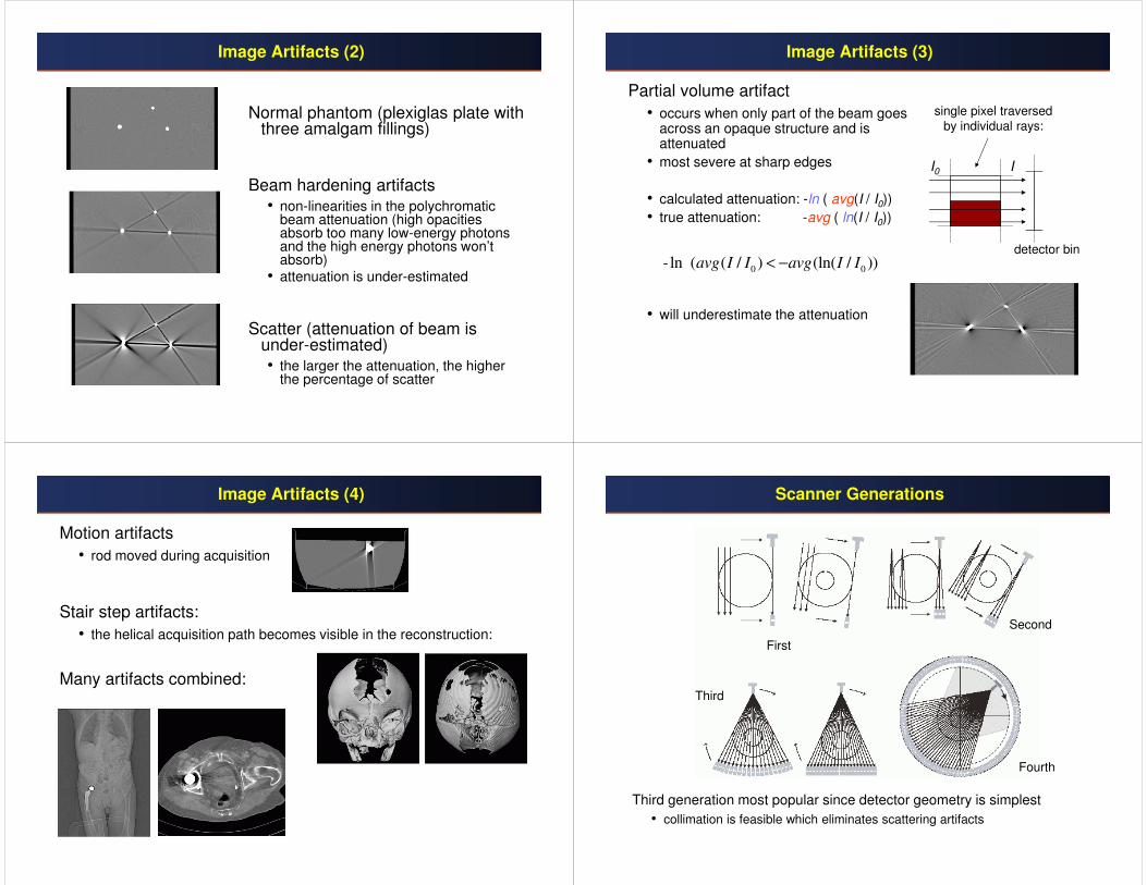
Image Artifacts (2)

Normal phantom (plexiglas plate with three amalgam fillings)

Beam hardening artifacts• non-linearities in the polychromatic

beam attenuation (high opacities absorb too many low-energy photons and the high energy photons won’t absorb)

• attenuation is under-estimated

Scatter (attenuation of beam is under-estimated)• the larger the attenuation, the higher

the percentage of scatter

Image Artifacts (3)

Partial volume artifact

• occurs when only part of the beam goes across an opaque structure and is attenuated

• most severe at sharp edges

• calculated attenuation: -ln ( avg(I / I0))

• true attenuation: -avg ( ln(I / I0))

• will underestimate the attenuation

0 0- ln ( ( / ) (ln( / )) avg I I avg I I< −detector bin

I0 I

single pixel traversed

by individual rays:

Image Artifacts (4)

Motion artifacts

• rod moved during acquisition

Stair step artifacts:

• the helical acquisition path becomes visible in the reconstruction:

Many artifacts combined:

Scanner Generations

Third generation most popular since detector geometry is simplest

• collimation is feasible which eliminates scattering artifacts

First

Second

Third

Fourth

Multislice CT

Nowadays (spiral) scanners are available that take up to 256 simultaneous slices (GE LightSpeed, Siemens, Phillips, Toshiba)

• require cone-beam algorithms for fully-3D reconstruction

• exact cone-beam algorithms have been recently developed

Multi-slice scanners enable faster scanning

• recall cone-beam?

• image lungs in 15s (one breath-hold)

• perform dynamic reconstructions of the heart (using gating)

• pick a certain phase of the heart cycle and reconstruct slabs in z

Single-slice Multi-slice

Multislice CT

Enables scanning of dynamic phenomena

• cardiac scanning

• lung scanning

Exotic Scanners: Dynamic Spatial Reconstructor

Dynamic Spatial Reconstructor (DSR)

• first fully 3D scanner, built in the 1980s by Richard Robb, Mayo Clinic

• 14 source-detector pairs rotating

• acquires data for 240 cross-sections at 60 volume/s

• 6 mm resolution (6 lp/cm)

Exotic Scanners: Electron Beam

Electron Beam Tomography (EBT)

• developed by Imatron, Inc

• currently 80 scanners in the world

• no moving mechanical parts

• ultra-fast (32 slices/s) and high resolution (1/4 mm)

• can image beating heart at high resolution

• also called cardiovascular CT CT (fifth generation CT)

CT: Final Remarks

Applications of CT• head/neck (brain, maxillofacial, inner ear, soft tissues of the neck)• thorax (lungs, chest wall, heart and great vessels)• urogenital tract (kidneys, adrenals, bladder, prostate, female genitals)• abdomen( gastrointestinal tract, liver, pancreas, spleen)• musceloskeletal system (bone, fractures, calcium studies, soft tissue

tumors, muscle tissue)

Biological effects and safety• radiation doses are relatively high in CT (effective dose in head CT is

2mSv, thorax 10mSv, abdomen 15 mSv, pelvis 5 mSv)• factor 10-100 higher than radiographic studies• proper maintenance of scanners a must

Future expectations• CT to remain preferred modality for imaging of the skeleton,

calcifications, the lungs, and the gastrointestinal tract• other application areas are expected to be replaced by MRI (see next

lectures)• low-dose CT and full cone-beam can be expected

Scanning: CSE 337: Introduction to Medical Imaging Lecture ...

Documents

Transcript of Scanning: CSE 337: Introduction to Medical Imaging Lecture ...