SCALING PROPERTIES OF STOCHASTIC PROCESSES WITH ...Scaling properties of stochastic processes refer...
122
Faculty of Science Department of Mathematics Danijel Grahovac SCALING PROPERTIES OF STOCHASTIC PROCESSES WITH APPLICATIONS TO PARAMETER ESTIMATION AND SAMPLE PATH PROPERTIES DOCTORAL THESIS Zagreb, 2015
Transcript of SCALING PROPERTIES OF STOCHASTIC PROCESSES WITH ...Scaling properties of stochastic processes refer...

Faculty of ScienceDepartment of Mathematics
Danijel Grahovac
SCALING PROPERTIES OF STOCHASTICPROCESSES WITH APPLICATIONS TO
PARAMETER ESTIMATION AND SAMPLEPATH PROPERTIES
DOCTORAL THESIS
Zagreb, 2015

Dan
ijelG
raho
vac
2015
DO
CTO
RA
LTH
ES
IS
Faculty of ScienceDepartment of Mathematics
Danijel Grahovac
SCALING PROPERTIES OF STOCHASTICPROCESSES WITH APPLICATIONS TO
PARAMETER ESTIMATION AND SAMPLEPATH PROPERTIES
DOCTORAL THESIS
Supervisors:Prof. Nikolai N. Leonenko
Izv. prof. dr. sc. Mirta Benšic
Zagreb, 2015

Prirodoslovno-matematicki fakultetMatematicki odsjek
Danijel Grahovac
SVOJSTVA SKALIRANJA SLUCAJNIHPROCESA S PRIMJENAMA U PROCJENI
PARAMETARA I SVOJSTVIMATRAJEKTORIJA
DOKTORSKI RAD
Mentori:Prof. Nikolai N. Leonenko
Izv. prof. dr. sc. Mirta Benšic
Zagreb, 2015.

Acknowledgements
First of all, I would like to thank my supervisor Prof. Nikolai Leonenko for his guidance,
constant support and many interesting and memorable discussions. His admiring enthu-
siasm and commitment will always be a source of inspiration to me. I thank to my second
supervisor, Prof. Mirta Ben²i¢ for her support and persistence in providing everything
to make my research possible. I thank to Nenad uvak, my dear colleague and friend for
his numerous advices and encouragements. I also thank to my collaborators, who shaped
many of the parts of this thesis.
I am grateful to my parents and my brother for always being there for me and believing
in me. A special thanks goes to my wife Maja for her love and understanding. Her constant
support and encouragement was in the end what made this work possible.
i

Summary
Scaling properties of stochastic processes refer to the behavior of the process at dierent
time scales and distributional properties of its increments with respect to aggregation. In
the rst part of the thesis, scaling properties are studied in dierent settings by analyz-
ing the limiting behavior of two statistics: partition function and the empirical scaling
function.
In Chapter 2 we study asymptotic scaling properties of weakly dependent heavy-tailed
sequences. These results are applied on the problem of estimation of the unknown tail
index. The proposed methods are tested against some existing estimators, such as Hill
and the moment estimator.
In Chapter 3 the same problem is analyzed for the linear fractional stable noise, which
is an example of a strongly dependent heavy-tailed sequence. Estimators will be developed
for the Hurst parameter and stable index, the main parameters of the linear fractional
stable motion.
Chapter 4 contains an overview of the theory of multifractal processes, which can
be characterized in several dierent ways. A practical problem of detecting multifractal
properties of time series is discussed from the point of view of the results of the preceding
chapters.
The last Chapter 5 deals with the ne scale properties of the sample paths described
with the so-called spectrum of singularities. The new results are given relating scaling
properties with path properties and applied to dierent classes of stochastic processes.
Keywords: partition function, scaling function, heavy-tailed distributions, tail in-
dex, linear fractional stable motion, Hurst parameter, multifractality, Hölder continuity,
spectrum of singularities
ii

Saºetak
Vaºnost svojstava skaliranja slu£ajnih procesa prvi je put istaknuta u radovima Benoita
Mandelbrota. Najpoznatije svojstvo skaliranja u teoriji slu£ajnih procesa je sebi-sli£nost.
Pojam multifraktalnosti pojavio se kasnije kako bi opisao modele s bogatijom strukturom
skaliranja. Jedan od na£ina kako se skaliranje moºe izu£avati jest kori²tenjem momenata
procesa i tzv. funkcije skaliranja. Multifraktalni procesi mogu se karakterizirati kao
procesi s nelinearnom funkcijom skaliranja. Ovaj pristup prirodno name¢e jednostavnu
metodu detekcije multifraktalnih svojstava procjenjivanjem funkcije skaliranja kori²tenjem
tzv. particijske funkcije.
Prvi dio ovog rada bavi se statisti£kim svojstvima takvih procjenitelja s obzirom
na razli£ite pretpostavke. Najprije ¢e se analizirati asimptotsko pona²anje empirijske
funkcije skaliranja za slu£aj slabo zavisnih nizova s te²kim repovima. Preciznije, pro-
matrat ¢e se stacionarni nizovi sa svojstvom eksponencijalno brzog jakog mije²anja koji
imaju marginalne distribucije u klasi distribucija s te²kim repovima. Dobiveni rezultati
bit ¢e iskori²teni za deniranje metoda procjene repnog indeksa te ¢e biti napravljena
usporedba s postoje¢im procjeniteljima kao ²to su Hillov i momentni procjenitelj. Osim
toga, predloºit ¢emo i gra£ku metodu temeljenu na obliku procijenjene funkcije skaliranja
koja moºe detektirati te²ke repove u uzorcima.
U sljede¢em koraku analizirat ¢e se asimptotska svojstva funkcije skaliranja na jako
zavisnim stacionarnim nizovima. Za primjer takvog niza koristit ¢emo linearni frakcionalni
stabilni ²um £ija svojstva su odreena s dva parametra, indeksom stabilnosti i Hurstovim
parametrom. Pokazat ¢emo da u ovom slu£aju funkcija skaliranja ovisi o vrijednostima
ta dva parametra. Na osnovu tih rezultata, denirat ¢e se metode za istodobnu procjenu
oba parametra koje predstavljaju alternativu standardnim procjeniteljima.
U drugom dijelu rada prethodno uspostavljeni rezultati ¢e biti analizirani s aspekta
multifraktalnih slu£ajnih procesa. U prvom redu, dobiveni rezultati pokazuju da nelin-
earnosti procijenjene funkcije skaliranja mogu biti posljedica te²kih repova distribucije
uzorka. Takav zaklju£ak dovodi u pitanje metodologiju temeljenu na particijskoj funkciji.
Svojstva skaliranja £esto se isprepli¢u sa svojstvima putova procesa. Osim u termin-
ima globalnih karakteristika kao ²to su momenti, multifraktalni slu£ajni procesi £esto se
deniraju i u terminima lokalnih nepravilnosti svojih trajektorija. Nepravilnosti u trajek-
torijama mogu se mjeriti formiranjem skupova vremenskih to£aka u kojima put procesa
iii

ima isti Hölderov eksponent u to£ki. Hausdorova dimenzija takvih skupova u ovisnosti
o Hölderovom eksponentu naziva se spektar singulariteta ili multifraktalni spektar. Mul-
tifraktalni slu£ajni procesi mogu se karakterizirati kao procesi koji imaju netrivijalan
spektar, u smislu da je spektar kona£an u vi²e od jedne to£ke. Dvije denicije mogu
se povezati tzv. multifraktalnim formalizmom koji predstavlja tvrdnju da su funkcija
skaliranja i spektar singulariteta Legendreova transformacija jedno drugoga. Brojna is-
traºivanja usmjerena su na uvjete pod kojima multifraktalni formalizam vrijedi. Spektar
singulariteta dosad je izveden za mnoge primjere slu£ajnih procesa, kao ²to su frakcionalno
Brownovo gibanje, Lévyjevi procesi i multiplikativne kaskade.
Rezultati o asimptotskom obliku funkcije skaliranja pokazat ¢e da u nekim slu£ajevima
procjena beskona£nih momenata moºe dati to£an spektar kori²tenjem multifraktalnog for-
malizma. Ova £injenica motivira dublje istraºivanje odnosa izmeu momenata i svojstava
trajektorija kojim se bavimo u posljednjem dijelu rada. Hölder neprekidnost i skaliranje
momenata povezani su poznatim Kolmogorovljevim teoremom neprekidnosti. S druge
strane, dokazat ¢emo svojevrsni komplement Kolmogorovljevog teorema koji povezuje
momente negativnog reda s izostankom Hölder neprekidnosti trajektorije u svakoj to£ki.
Ova tvrdnja bit ¢e dodatno poja£ana formulacijom u terminima momenata negativnog
reda maksimuma nekog ksnog broja prirasta procesa. Iz ovih rezultata, izmeu ostalog,
slijedit ¢e da sebi-sli£ni procesi s kona£nim momentima imaju trivijalan spektar (npr. frak-
cionalno Brownovo gibanje). Obratno, svaki sebi-sli£an proces s netrivijalnim spektrom
mora imati te²ke repove (npr. stabilni Lévyjevi procesi). Dobiveni rezultati sugeriraju
prirodnu modikaciju particijske funkcije koja ¢e biti testirana na nizu primjera.
Klju£ne rije£i: particijska funkcija, funkcija skaliranja, distribucije s te²kim re-
povima, repni indeks, linearno frakcionalno stabilno gibanje, Hurstov parametar, mul-
tifraktalnost, Hölder neprekidnost, spektar singulariteta
iv

Contents
Acknowledgements i
Summary ii
Saºetak iii
1 Introduction 1
1.1 Partition function . . . . . . . . . . . . . . . . . . . . . . . . . . . . . . . . 2
1.2 Empirical scaling function . . . . . . . . . . . . . . . . . . . . . . . . . . . 3
1.3 Overview . . . . . . . . . . . . . . . . . . . . . . . . . . . . . . . . . . . . . 4
2 Asymptotic scaling of weakly dependent heavy-tailed stationary sequences 5
2.1 Asymptotic scaling . . . . . . . . . . . . . . . . . . . . . . . . . . . . . . . 5
2.1.1 Assumptions . . . . . . . . . . . . . . . . . . . . . . . . . . . . . . . 5
2.1.2 Main theorems . . . . . . . . . . . . . . . . . . . . . . . . . . . . . 7
2.1.3 Proofs of Theorems 1 and 2 . . . . . . . . . . . . . . . . . . . . . . 11
2.2 Applications in the tail index estimation . . . . . . . . . . . . . . . . . . . 22
2.2.1 Overview of the existing methods . . . . . . . . . . . . . . . . . . . 23
2.2.2 Graphical method . . . . . . . . . . . . . . . . . . . . . . . . . . . . 25
2.2.3 Plots of the empirical scaling functions . . . . . . . . . . . . . . . . 25
2.2.4 Estimation methods . . . . . . . . . . . . . . . . . . . . . . . . . . 28
2.2.5 Simulation study . . . . . . . . . . . . . . . . . . . . . . . . . . . . 32
2.2.6 Examples and comparison . . . . . . . . . . . . . . . . . . . . . . . 36
3 Asymptotic scaling of the linear fractional stable noise 40
3.1 Linear fractional stable motion . . . . . . . . . . . . . . . . . . . . . . . . . 40
3.2 Asymptotic scaling . . . . . . . . . . . . . . . . . . . . . . . . . . . . . . . 42
3.3 Applications in parameter estimation . . . . . . . . . . . . . . . . . . . . . 47
3.3.1 Estimation methods . . . . . . . . . . . . . . . . . . . . . . . . . . 49
3.3.2 Simulation study . . . . . . . . . . . . . . . . . . . . . . . . . . . . 51
3.3.3 Real data applications . . . . . . . . . . . . . . . . . . . . . . . . . 54
v

Contents
4 Detecting multifractality of time series 56
4.1 Multifractal stochastic processes . . . . . . . . . . . . . . . . . . . . . . . . 56
4.1.1 Denitions of multifractality . . . . . . . . . . . . . . . . . . . . . . 57
4.1.2 Spectrum of singularities . . . . . . . . . . . . . . . . . . . . . . . . 63
4.1.3 Multifractal formalism . . . . . . . . . . . . . . . . . . . . . . . . . 66
4.2 Statistical analysis of multifractal processes . . . . . . . . . . . . . . . . . . 68
4.3 Detecting multifractality under heavy tails . . . . . . . . . . . . . . . . . . 70
4.3.1 Estimation of the spectrum . . . . . . . . . . . . . . . . . . . . . . 73
4.4 Simulations and examples . . . . . . . . . . . . . . . . . . . . . . . . . . . 75
4.4.1 Example 1 . . . . . . . . . . . . . . . . . . . . . . . . . . . . . . . . 75
4.4.2 Example 2 . . . . . . . . . . . . . . . . . . . . . . . . . . . . . . . . 76
4.4.3 Conclusion . . . . . . . . . . . . . . . . . . . . . . . . . . . . . . . . 78
5 Moments and the spectrum of singularities 81
5.1 Motivation . . . . . . . . . . . . . . . . . . . . . . . . . . . . . . . . . . . . 81
5.1.1 Negative order moments . . . . . . . . . . . . . . . . . . . . . . . . 83
5.2 Bounds on the support of the spectrum . . . . . . . . . . . . . . . . . . . . 84
5.2.1 The lower bound . . . . . . . . . . . . . . . . . . . . . . . . . . . . 84
5.2.2 The upper bound . . . . . . . . . . . . . . . . . . . . . . . . . . . . 86
5.3 Applications . . . . . . . . . . . . . . . . . . . . . . . . . . . . . . . . . . . 91
5.3.1 The case of self-similar stationary increments processes . . . . . . . 91
5.3.2 The case of multifractal processes . . . . . . . . . . . . . . . . . . . 93
5.4 Examples . . . . . . . . . . . . . . . . . . . . . . . . . . . . . . . . . . . . 94
5.4.1 Self-similar processes . . . . . . . . . . . . . . . . . . . . . . . . . . 95
5.4.2 Lévy processes . . . . . . . . . . . . . . . . . . . . . . . . . . . . . 97
5.4.3 Multifractal processes . . . . . . . . . . . . . . . . . . . . . . . . . . 98
5.5 Robust version of the partition function . . . . . . . . . . . . . . . . . . . . 99
Bibliography 103
Curriculum vitae 111
vi

Chapter 1
Introduction
The importance of scaling relations was rst stressed in the work of Benoit Mandelbrot.
The early references are the seminal papers Mandelbrot (1963) and Mandelbrot (1967); see
also Mandelbrot (1997). Scaling properties of stochastic processes refer to the behavior of
the process at dierent time scales. This usually accounts to changes in nite dimensional
distributions of the process when the time parameter is scaled by some factor. The best
known scaling relation in the theory of stochastic processes is self-similarity. The scaling
of time of the self-similar processes by some constant a > 0 results in scaling the state
space by a factor b > 0, in the sense of nite dimensional distributions. More precisely,
a stochastic process X(t), t ≥ 0 is said to be self-similar if for any a > 0 there exists
b > 0 such that
X(at) d= bX(t),
where equality is in nite dimensional distributions. Suppose X(t) is self-similar, non-
trivial (meaning it is not a.s. constant for every t) and stochastically continuous at 0,
that is for every ε > 0, P (|X(t)−X(0)| > ε) → 0 as t → 0. Then b must be of the form
aH for some H ≥ 0, i.e.
X(at) d= aHX(t).
Constant H is called the Hurst parameter or the self-similarity index. The importance of
self-similar processes may be illustrated by the Lamperti's theorem, which states that the
only possible limit (in the sense of nite dimensional distributions) of a normalized partial
sum process of stationary sequences are self-similar processes with stationary increments
(see Embrechts & Maejima (2002) for more details).
As a generalization of self-similarity, models allowing a richer form of scaling were
introduced by Yaglom as measures to model turbulence (Yaglom (1966)). Later these
models were called multifractal in the work of Frisch and Parisi (Frisch & Parisi (1985)).
The concept can be easily generalized to stochastic processes, thus extending the notion
of self-similar processes by allowing the factor aH to be random. Of course, in many
examples there is no such exact scaling of nite dimensional distributions as in the case
1

Chapter 1. Introduction
of self-similar or multifractal processes.
If we have a sequence of random variables (Yi, i ∈ N), then we can also speak about
scaling properties of the partial sum process ∑n
i=1 Yi, n ∈ N. For example, if (Yi, i ∈ N)is an independent identically distributed (i.i.d.) sequence with strictly α-stable distribu-
tion, α ∈ (0, 2], then we know that
n∑i=1
Yid= n1/αY1, ∀n ∈ N. (1.1)
The continuous time analog of this case corresponds to Brownian motion (α = 2) and
strictly α-stable Lévy processes, which are both self-similar with Hurst parameter 1/α.
This parameter appears by taking logarithms in (1.1)
ln |∑n
i=1 Yi|lnn
d= 1/α+
ln |Y1|lnn
, ∀n ∈ N,
and represents the rate of growth of the partial sum process measured as a power of n.
The central limit theorem indicates that for all zero mean (if mean exists) i.i.d. sequences
the relation (1.1) holds approximately for large n. Thus, in the general case, scaling can
be studied as the behavior of the sequence with respect to aggregation and measured as
the rate of growth of the partial sums.
We adopt this point of view and in the next section we dene the so-called partition
function (sometimes called empirical structure function). Partition function will be used
for dening the so-called empirical scaling function. The names of the two come from the
theory of multifractal processes, which is a topic we deal with in Chapter 4.
1.1 Partition function
Partition function is a special kind of the sample moment statistic based on the blocks of
data. Given a sequence of random variables Y1, Y2, . . . we dene the partition function to
be
Sq(n, t) =1
⌊n/t⌋
⌊n/t⌋∑i=1
∣∣∣∣∣∣⌊t⌋∑j=1
Y(i−1)⌊t⌋+j
∣∣∣∣∣∣q
, (1.2)
where q ∈ R and 1 ≤ t ≤ n. In words, we partition the data into consecutive blocks
of length ⌊t⌋, we sum each block and take the power q of the absolute value of the sum.
Finally, we average over all ⌊n/t⌋ blocks. Notice that for t = 1 one gets the usual empirical
q-th absolute moment.
The partition function can also be viewed as an estimator of the q-th absolute moment
of the process with stationary increments. Indeed, suppose X(t) is a process with
stationary increments and one tries to estimate E|X(t)|q for xed t > 0 based on a
2

Chapter 1. Introduction
discretely observed sample Xi = X(i), i = 1, . . . , n. The natural estimator is given by
1
⌊n/t⌋
⌊n/t⌋∑i=1
∣∣Xi⌊t⌋ −X(i−1)⌊t⌋∣∣q .
If we denote the one step increments as Yi = X(i)−X(i− 1), then this is equal to (1.2).
In Chapters 2 and 3 we will study asymptotic properties of the partition function in
two settings. Instead of keeping t xed, we take it to be of the form t = ns for some
s ∈ (0, 1), which allows the blocks to grow as the sample size increases. The partition
function will then have the following form
Sq(n, ns) =
1
⌊n1−s⌋
⌊n1−s⌋∑i=1
∣∣∣∣∣∣⌊ns⌋∑j=1
Y⌊ns⌋(i−1)+j
∣∣∣∣∣∣q
. (1.3)
Since s > 0, Sq(n, ns) will generally diverge as n → ∞. We are interested in the rate of
divergence of this statistic measured as a power of n. This can be obtained by considering
the limiting behavior oflnSq(n, n
s)
lnn
as n → ∞. One can think of this limiting value as the value of the smallest power of n
needed to normalize the partition function in such a way that it will converge to some
random variable not identically equal to zero.
1.2 Empirical scaling function
If X(t) is aH-self-similar process with stationary increments, then E|X(t)|q = tHqE|X(1)|q
for q ∈ R such that E|X(t)|q < ∞. Taking logarithms we have that
lnE|X(t)|q = Hq ln t+ lnE|X(1)|q.
Having in mind that Sq(n, t) can be considered as the estimator of E|X(t)|q, we can expectthat lnSq(n, t) will be linear in ln t. This motivates considering the slope in the simple
linear regression of lnSq(n, t) on ln t based on some points 1 ≤ ti ≤ n, i = 1, . . . , N . These
slopes for varying q will be called the empirical scaling function, although linear relation
may not always be justied.
Given points 1 ≤ ti ≤ n, i = 1, . . . , N and using the well known formula for the slope
of the linear regression line, we dene the empirical scaling function at the point q as
τN,n(q) =
∑Ni=1 ln ti lnSq(n, ti)− 1
N
∑Ni=1 ln ti
∑Nj=1 lnSq(n, tj)∑N
i=1 (ln ti)2 − 1
N
(∑Ni=1 ln ti
)2 . (1.4)
3

Chapter 1. Introduction
If we write ti in the form nsi , si ∈ (0, 1), i = 1, . . . , N , then the empirical scaling function
is given by
τN,n(q) =
∑Ni=1 si
lnSq(n,nsi )
lnn− 1
N
∑Ni=1 si
∑Nj=1
lnSq(n,nsj )
lnn∑Ni=1 (si)
2 − 1N
(∑Ni=1 si
)2 . (1.5)
1.3 Overview
The partition function and the empirical scaling function will be used to study asymptotic
scaling properties of dierent types of stationary sequences. In the next chapter we
establish asymptotic behavior for weakly dependent heavy-tailed sequences and in Chapter
3 we do the same analysis for the linear fractional stable noise, which is an example of
a heavy-tailed and strongly dependent sequence. Both results will have applications in
the parameter estimation problem. In the rst setting, we will propose an exploratory
method and several estimation methods for the unknown tail index that will be compared
with the existing estimators. In the second setting we establish methods for estimating
Hurst exponent and stable index of the linear fractional stable motion.
In Chapter 4 we provide an overview of the theory of multifractal processes and con-
sider the implications of the results of Chapters 2 and 3. The analysis will lead to a
conclusion that, empirically, it is hard to distinguish multifractal and heavy-tailed pro-
cesses. In Chapter 5 we study in more details the relation between ne path properties and
moments of both positive and negative order. Such analysis will lead to a new denition
of the partition function.
4

Chapter 2
Asymptotic scaling of weakly
dependent heavy-tailed stationary
sequences
In this chapter we establish limiting behavior of the partition function and the empirical
scaling function introduced in (1.3) and (1.5). The results are applied in the tail index
estimation problem, which is discussed in Section 2.2.
2.1 Asymptotic scaling
In order to establish our results, we rst summarize the assumptions on the sequences
considered in this chapter.
2.1.1 Assumptions
Through the chapter we assume that (Yi, i ∈ N) is a strictly stationary sequence of randomvariables. Each Yi is assumed to have a heavy-tailed distribution with tail index α. This
means that it has a regularly varying tail with index −α so that
P (|Yi| > x) =L(x)
xα,
where L(t), t > 0 is a slowly varying function, that is, for every t > 0, L(tx)/L(x) → 1
as x → ∞. In particular, this implies that E|X|q < ∞ for 0 < q < α and E|X|q = ∞for q > α, which is sometimes also used to dene heavy tails. The parameter α is
called the tail index and measures the thickness of the tails. Examples of heavy-tailed
distributions include Pareto, stable and Student's t-distribution, which will be precisely
dened in Subsections 2.2.3 and 2.2.5. For more details on heavy-tailed distributions,
regular variation and related topics see Embrechts et al. (1997) and Resnick (2007).
5

Chapter 2. Asymptotic scaling of weakly dependent heavy-tailed stationary sequences
We also impose some assumptions on the dependence structure of the sequence, which
go beyond the independent case. First, for two sub-σ-algebras, A ⊂ F and B ⊂ F on the
same complete probability space (Ω,F , P ) we dene
a(A,B) = supA∈A,B∈B
|P (A ∩B)− P (A)P (B)|.
Now for a process Yt, t ∈ N or Yt, t ∈ [0,∞), consider Ft = σYs, s ≤ t and
F t+τ = σYs, s ≥ t + τ. We say that Yt has a strong mixing property if a(τ) =
supt≥0 a(Ft,F t+τ ) → 0 as τ → ∞. Strong mixing is sometimes also called α-mixing. If
a(τ) = O(e−bτ ) for some b > 0 we say that the strong mixing property has an exponentially
decaying rate. We will refer to a(τ) as the strong mixing coecient function. Through this
chapter (Yi, i ∈ N) is assumed to have the strong mixing property with an exponentially
decaying rate.
In some arguments the proof of the main result of this chapter relies on the limit theory
for partial maxima of absolute values of the sequence (Yi, i ∈ N). It is well known that for
the i.i.d. sequence (Zi, i ∈ N) having regularly varying tail with index −α there exists a se-
quence of the form n1/αL1(n) with L1 slowly varying, such thatmaxi=1,...,n |Zi|/(n1/αL1(n))
converges in distribution to a Fréchet random variable whose distribution is one of the
three types of distributions that can occur as a limit law for maxima (see Embrechts
et al. (1997) for more details). Following Leadbetter et al. (1982), this can be extended to
weakly dependent stationary sequence (Yi, i ∈ N) under additional assumptions. We say
that (Yi, i ∈ N) has extremal index θ if for each τ > 0 there exists a sequence un(τ) such
that nP (|Y1| > un(τ)) → τ and P (maxi=1,...,n |Yi| ≤ un(τ)) → e−θτ as n → ∞. If (Yi) is
strong mixing and Yi heavy-tailed, then it is enough for this to hold for a single τ > 0 in
order for θ to be the extremal index. It always holds that θ ∈ [0, 1]. The i.i.d. sequence
(Zi, i ∈ N) such that Zi =d Yi for each i is called the associated independent sequence. If
θ > 0, then the limiting distribution of maxi=1,...,n |Yi| is of the same type as the limit of
the maximum of the associated independent sequence with the same norming constants.
In particular, if θ > 0, under our assumptions maxi=1,...,n |Yi|/(n1/αL1(n)) converges in
distribution to a Fréchet random variable, possibly with dierent scale parameter. For
our consideration in this chapter, we assume (Yi, i ∈ N) has positive extremal index. The
case when θ = 0 or does not exist is considered as degenerate and only a few examples are
known where this happens under some type of mixing condition assumed (see (Leadbetter
et al. 1982, Chapter 3) and references therein). In particular, θ > 0 holds for any example
considered later in this chapter.
6
Chapter 2. Asymptotic scaling of weakly dependent heavy-tailed stationary sequences
2.1.2 Main theorems
Asymptotic properties of the partition function Sq(n, t) have been considered before in
the context of multifractality detection (Heyde (2009), Sly (2005); see also Heyde & Sly
(2008)). Notice that if we keep t xed, behavior of Sq(n, t) as n → ∞ accounts to the
standard limit theory for partial sums of the sequence∣∣∣∣∣∣⌊t⌋∑j=1
Y(i−1)⌊t⌋+j
∣∣∣∣∣∣q
, i = 1, 2, . . . . (2.1)
If (Yi, i ∈ N) is i.i.d. and q < α, the weak law of large numbers implies that Sq(n, t)
converges in probability to the expectation of (2.1) as n → ∞. To get more interesting
limit results and analyze the eect of the block size, we take t = ns. It is clear that
Sq(n, ns) will diverge as n → ∞ and we will measure the rate of divergence of this statistic
as a power of n. To obtain the limiting value, we analyze lnSq(n, ns)/ lnn representing
the rate of growth.
The next theorem summarizes the main results on the rate of growth. We additionally
assume that the sequence has a zero expectation in case α > 1. For practical purposes,
this is not a restriction as one can always subtract the mean from the starting sequence.
For the case α ≤ 1 this is not necessary. The proof of the theorem is given in Subsection
2.1.3. A special case of this theorem has been proved in Sly (2005) and cited in Heyde
(2009).
Theorem 1. Let (Yi, i ∈ N) be a strictly stationary sequence that has a strong mixing
property with an exponentially decaying rate, positive extremal index and suppose that
Yi, i ∈ N has a heavy-tailed distribution with tail index α > 0. Suppose also that EYi = 0
if α > 1. Then for every q > 0 and every s ∈ (0, 1)
lnSq(n, ns)
lnn
P→ Rα(q, s) :=
sqα, if q ≤ α and α ≤ 2,
s+ qα− 1, if q > α and α ≤ 2,
sq2, if q ≤ α and α > 2,
maxs+ q
α− 1, sq
2
, if q > α and α > 2,
(2.2)
as n → ∞, whereP→ stands for convergence in probability.
In order to illustrate the eects of the theorem, consider the simple case in which
(Yi, i ∈ N) is a zero mean (if α > 1) i.i.d. sequence that is in the domain of normal
attraction of some α-stable random variable, 0 < α < 2. This means that∑n
i=1 Yi/n1/α
converges in distribution to some random variable Z with α-stable distribution. A su-
cient condition for this to hold is the regular variation of the tail (2.1.1) with L constant
7

Chapter 2. Asymptotic scaling of weakly dependent heavy-tailed stationary sequences
at innity and the balance of the tails (see Gnedenko & Kolmogorov (1968) for more
details). Suppose rst that q < α and notice that
Sq(n, ns)
nsqα
=1
⌊n1−s⌋
⌊n1−s⌋∑i=1
∣∣∣∣∣∑⌊ns⌋
j=1 Y⌊ns⌋(i−1)+j
nsα
∣∣∣∣∣q
.
When n → ∞, each of the internal sums converges in distribution to an independent copy
of Z. Since q < α, E|Z|q is nite, so the weak law of large numbers applies and shows
that the average tends to some nonzero and nite limit. For the case q > α, the weak law
cannot be applied and the rate of growth will be higher:
Sq(n, ns)
ns+ qα−1
=
∑⌊n1−s⌋i=1
∣∣∣∣∑⌊ns⌋j=1 Y⌊ns⌋(i−1)+j
nsα
∣∣∣∣qn(1−s) q
α
.
Internal sums again converge to independent copies of Z. Since |Z|q has (−α/q)-regularly
varying tail, it will be in the domain of attraction of (α/q)-stable distribution. Centering is
not necessary since α/q < 1 and the limit (modulo possibly some slowly varying function)
will be some positive random variable.
For the case α > 2, the variance is nite and so the central limit theorem holds. When
q < α the rate of growth has an intuitive explanation by arguments similar to those just
given above. When q > α, interesting things happen. Note that the asymptotics of the
partition function is inuenced by two factors: averaging and the weak law on the one
side and distributional limit arguments on the other side. It will depend on s which of
the two inuences prevails. For larger s, s+ q/α− 1 < sq/2 and the rate will be as in the
case q < α, i.e.,
Sq(n, ns)
nsq2
=1
⌊n1−s⌋
⌊n1−s⌋∑i=1
∣∣∣∣∣∑⌊ns⌋
j=1 Y⌊ns⌋(i−1)+j
ns2
∣∣∣∣∣q
.
Internal sums converge in distribution to normal, which has every moment nite and
the weak law applies. But for small s, the rate will be the same as that for the case
α < 2. What happens is that in this case internal sums have a small number of terms,
so convergence to normal is slow, much slower than the eect of averaging. This is the
reason why the rate is greater than sq/2.
Remark 1. Note that in general, the normalizing sequence for partial sums can be of the
form n1/αL(n) for some slowly varying function L. This does not aect the rate of growth.
Indeed, if Zn/naL(n) →d Z for some non-negative sequence Zn, then for every ε > 0,
P
(lnZn
lnn< a− ε
)= P
(Zn < na−ε
)= P
(Zn
naL(n)<
1
L(n)nε
)≤ P
(Zn
naL(n)<
1
2nε
)→ 0,
8

Chapter 2. Asymptotic scaling of weakly dependent heavy-tailed stationary sequences
since for n large enough n−ε < L(n) < nε, i.e. lnL(n)/ lnn → 0. Similar argument
applies for the upper bound. On the other hand, if lnZn/ lnn →P a, then Zn grows
at the rate a in the sense that for every ε > 0 there exist constants c1, c2 > 0 such
that P (c1 < Zn/na < c2) ≥ 1 − ε for n large enough. This is sometimes denoted as
Zn = ΘP (na).
Remark 2. A natural question arises from the previous discussion whether it is possible
to identify a normalizing sequence and a distributional limit of Sq(n, ns). In some special
cases the limit can be easily deduced. Suppose (Yi, i ∈ N) is an i.i.d. sequence with
strictly α-stable distribution. When q < α, the rate of growth will be sq/α. Dividing the
partition function with nsq/α and using the scaling property of stable distributions yields
Sq(n, ns)
nsqα
=1
⌊n1−s⌋
⌊n1−s⌋∑i=1
∣∣∣∣∣∑⌊ns⌋
j=1 Y⌊ns⌋(i−1)+j
nsα
∣∣∣∣∣q
d=
1
⌊n1−s⌋
⌊n1−s⌋∑i=1
|Yi|q .
Since q < α, E|Yi|q < ∞ and the weak law of large numbers implies
Sq(n, ns)
nsqα
P→ E|Y1|q, n → ∞.
On the other hand, when q ≥ α the weak law cannot be applied and the rate of growth
is s+ q/α− 1. Normalizing the partition function gives
Sq(n, ns)
ns+ qα−1
=
∑⌊n1−s⌋i=1
∣∣∣∣∑⌊ns⌋j=1 Y⌊ns⌋(i−1)+j
nsα
∣∣∣∣qn(1−s) q
α
d=
∑⌊n1−s⌋i=1 |Yi|q
n(1−s) qα
.
Each |Yi|q has (−α/q) regularly varying tail, so it will be in the domain of normal attrac-
tion of (α/q)-stable distribution. Since α/q < 1, the centering is not needed and by the
generalized central limit theorem it follows that
Sq(n, ns)
ns+ qα−1
d→ Z, n → ∞,
with Z having (α/q)-stable distribution.
Using Theorem 1 we can establish asymptotic properties of the empirical scaling func-
tion dened by (1.5). First, we show how Theorem 1 can motivate the denition of the
scaling function.
Using the notation of Theorem 1, we denote
εn :=Sq(n, n
s)
nRα(q,s).
9

Chapter 2. Asymptotic scaling of weakly dependent heavy-tailed stationary sequences
Taking logarithms and rewriting yields
lnSq(n, ns)
lnn= Rα(q, s) +
ln εnlnn
. (2.3)
As follows from Remark 1, εn is bounded in probability from above and from bellow, thus,
it makes sense to view (2.3) as a regression model of lnSq(n, ns)/ lnn on q and s with
the model function Rα(q, s), where ln εn/ lnn are the errors. One should count on the
intercept in the model due to the possible nonzero mean of an error. Notice that, when
α ≤ 2, Rα(q, s) is linear in s, i.e. it can be written in the form Rα(q, s) = a(q)s+ b(q) for
some functions a(q) and b(q). This also holds if α > 2 and q ≤ α. We can then rewrite
(2.3) aslnSq(n, n
s)
lnn= a(q)s+ b(q) +
ln εnlnn
.
Fixing q gives the simple linear regression model of lnSq(n, ns)/ lnn on s, thus it makes
sense to consider the slope of this regression. This is exactly the empirical scaling function
(1.5). If α > 2 and q > α, Rα(q, s) is not linear in s due to the maximum term in (2.2). It
is actually a broken line with the breakpoint depending on the values of q and α. However,
this does not prevent us from considering statistic (1.5) anyway. This will be reected as
the peculiar nonlinear shape of the asymptotic scaling function.
Theorem 2. Suppose that the assumptions of Theorem 1 hold and τN,n is the empirical
scaling function based on the points s1, . . . , sN ∈ (0, 1). Let
τ∞α (q) =
qα, if q ≤ α and α ≤ 2,
1, if q > α and α ≤ 2,
q2, if 0 < q ≤ α and α > 2,
q2+ 2(α−q)2(2α+4q−3αq)
α3(2−q)2, if q > α and α > 2.
(2.4)
(i) If α ≤ 2 or α > 2 and q ≤ α then
plimn→∞
τN,n(q) = τ∞α (q),
where plim stands for the limit in probability.
(ii) If α > 2 and q > α, suppose si = i/N , i = 1 . . . , N . Then
limN→∞
plimn→∞
τN,n(q) = τ∞α (q).
Theorem 2 shows that, asymptotically, the shape of the empirical scaling function in
the setting considered signicantly depends on the value of the tail index α. The limit
from case (i) of Theorem 2 does not depend on the choice of points si in the computation
10

Chapter 2. Asymptotic scaling of weakly dependent heavy-tailed stationary sequences
of the empirical scaling function. In case (ii), we need additional assumptions as in this
case we are estimating the slope while the underlying relation is actually nonlinear. Plots
of the asymptotic scaling function τ∞α for dierent values of α are shown in Figure 2.1.
When α ≤ 2, the scaling function has the shape of a broken line (we will refer to this
shape as bilinear). In this case the rst part of the plot is a line with slope 1/α > 1/2
and the second part is a horizontal line with value 1. A break occurs exactly at the point
α. In case α > 2, τ∞α is approximately bilinear, the slope of the rst part is 1/2 and
again the breakpoint is at the α. When α is large, i.e., α → ∞, it follows from (2.4)
that τ∞α (q) ≡ q/2. This case corresponds to a sequence coming from a distribution with
all moments nite, e.g., an independent normally distributed sample. This line will be
referred to as the baseline. In Figure 2.1 the baseline is shown by a dashed line. The
cases α ≤ 2 (α = 0.5, 1, 1.5) and α > 2 (α = 2.5, 3, 3.5, 4) are shown by dot-dashed and
solid lines, respectively.
2 4 6 8 10q
1
2
3
4
5
ΤΑ
¥HqL
43.53.2.51.510.5Α
Figure 2.1: Plots of τ∞α for dierent values of α
2.1.3 Proofs of Theorems 1 and 2
One of the main ingredients in the proof of Theorem 1 is the following version of Rosen-
thal's inequality for strong mixing sequences, precisely Theorem 2 in Section 1.4.1 of
Doukhan (1994):
Lemma 1. Fix q > 0 and suppose (Zk, k ∈ N) is a sequence of random variables and let
aZ(m) be the corresponding strong mixing coecient function. Suppose that there exists
ζ > 0 and c ≥ q, c ∈ N such that
∞∑m=1
(m+ 1)2c−2 (aZ(m))ζ
2c+ζ < ∞, (2.5)
and suppose E|Zk|q+ζ < ∞ and if q > 1, EZk = 0 for all k. Then there exists some
11

Chapter 2. Asymptotic scaling of weakly dependent heavy-tailed stationary sequences
constant K depending only on q and aZ(m) such that
E
∣∣∣∣∣l∑
k=1
Zk
∣∣∣∣∣q
≤ KD(q, ζ, l),
where
D(q, ζ, l) =
L(q, 0, l), if 0 < q ≤ 1,
L(q, ζ, l), if 1 < q ≤ 2,
maxL(q, ζ, l), (L(2, ζ, l))
q2
, if q > 2,
L(q, ζ, l) =l∑
k=1
(E |Zk|q+ζ
) qq+ζ
.
Remark 3. The inequality from Lemma 1 for q ≤ 1 is a simple consequence of the fact
that for 0 < q ≤ 1, (a+b)q ≤ aq+bq for all a, b ≥ 0. Therefore, in this case no assumption
on the mixing is needed and more importantly Zk are not required to be centered.
Proof of Theorem 1. We split the proof into three parts depending whether q > α, q < α
or q = α.
(a) Let q > α. First we show an upper bound for the limit in probability.
Let ϵ > 0. Notice that
nlnSq(n,ns)
lnn = Sq(n, ns) =
1
⌊n1−s⌋
⌊n1−s⌋∑i=1
∣∣∣∣∣∣⌊ns⌋∑j=1
Y⌊ns⌋(i−1)+j
∣∣∣∣∣∣q
.
Let δ > 0 and dene
Yj,n = Yj 1(|Yj| ≤ n
1α+δ), j = 1, . . . , n, n ∈ N,
Zj,n = Yj,n − EYj,n,
ξi =
∣∣∣∣∣∣⌊ns⌋∑j=1
Zns(i−1)+j,n
∣∣∣∣∣∣q
, i = 1, . . . , ⌊n1−s⌋.
By Remark 3, centering is not needed in Lemma 1 when α < q ≤ 1 and so we consider
Zj,n = Yj,n in this case. Before splitting the cases based on dierent α values, we derive
some facts that will be used later. Due to stationarity, (ξi) are identically distributed for
xed n, so that E[(1/k)
∑ki=1 ξi
]= Eξ1. Moments of all orders of Yj,n are nite and by
using Karamata's theorem (Resnick 2007, Theorem 2.1), for arbitrary r > α it follows
12

Chapter 2. Asymptotic scaling of weakly dependent heavy-tailed stationary sequences
that for n large enough
E|Yj,n|r =∫ ∞
0
P (|Yj,n|r > x)dx =
∫ nr( 1α+δ)
0
P (|Yj|r > x)dx
=
∫ nr( 1α+δ)
0
L(x1r )x−α
r dx ≤ C1L(n1α+δ)nr( 1
α+δ)(−α
r+1) ≤ C1n
rα−1+δ(r−α)+η,
(2.6)
since for any η > 0 we can take n large enough to make L(n1/α+δ) ≤ nη. It follows then
that if r > 1 by Jensen's inequality
E|Zj,n|r = E|Yj,n − EYj,n|r ≤ 2r−1(E|Yj,n|r + (E|Yj,n|)r
)≤ 2rE|Yj,n|r
≤ C2nrα−1+δ(r−α)+η.
(2.7)
On the other hand, if r ≤ 1, the same bound holds as α < r ≤ 1 so there is no centering,
i.e. E|Zj,n|r = E|Yj,n|r.Next, notice that, for xed n, Zj,n, j = 1, . . . , n is a stationary sequence. By denition
EZj,n = 0 and also E|Zj,n|q+ζ < ∞ for every ζ > 0. Since Zj,n is no more than a
measurable transformation of Yj, the mixing properties of Zj,n are inherited from those
of sequence (Yj). This means that there exists a constant b > 0 such that the mixing
coecients sequence satises aZ(m) = O(e−bm) as m → ∞. It follows that
∞∑m=1
(m+ 1)2c−2 (aZ(m))ζ
2c+ζ ≤∞∑
m=1
(m+ 1)2c−2K1e−bm ζ
2c+ζ < ∞
for every choice of c ∈ N and ζ > 0. Hence we can apply Lemma 1 for n xed to get
Eξ1 = E
∣∣∣∣∣∣⌊ns⌋∑j=1
Zj,n
∣∣∣∣∣∣q
≤
KL(q, 0, ⌊ns⌋), if 0 < q ≤ 1,
KL(q, ζ, ⌊ns⌋), if 1 < q ≤ 2,
KmaxL(q, ζ, ⌊ns⌋), (L(2, ζ, ⌊ns⌋))
q2
, if q > 2.
(2.8)
Notice that none of the previous arguments uses assumptions on α. Now we split the cases:
•α > 2 Because for q > α, utilizing Equation (2.7), we can choose ζ small enough so
that ζ < qδα (in order to achieve n− qq+ζ
(1+δα) < n−1) to obtain
L(q, ζ, ⌊ns⌋) =⌊ns⌋∑j=1
(E |Zj,n|q+ζ
) qq+ζ ≤ C3n
sn(q+ζα
−1+δ(q+ζ−α)+η)( qq+ζ )
≤ C3ns+ q
α− q
q+ζ(1+δα)+δq+η ≤ C3n
s+ qα−1+δq+η, (2.9)
13

Chapter 2. Asymptotic scaling of weakly dependent heavy-tailed stationary sequences
and
(L(2, ζ, ⌊ns⌋))q2 =
⌊ns⌋∑j=1
(E |Zj,n|2+ζ
) 22+ζ
q2
≤ nsq2
(E|Y1|2+ζ
) q2+ζ ≤ C4n
sq2 .
Hence Eξ1 ≤ C5nmaxs+ q
α−1+δq+η, sq
2 .
•1 < α ≤ 2 Bound for L(q, ζ, ⌊ns⌋) is the same as in (2.9), so if α < q ≤ 2 we have
Eξ1 ≤ KL(q, ζ, ⌊ns⌋) ≤ C5ns+q/α−1+δq+η. If q > 2, using Equation (2.7) and choosing
ζ < 2δα yields
(L(2, ζ, ⌊ns⌋))q2 =
⌊ns⌋∑j=1
(E |Zj,n|2+ζ
) 22+ζ
q2
≤ nsq2
(C2n
2+ζα
−1+δ(2+ζ−α)+η) q
2+ζ
≤ C6nsq2+ q
α− q
2+ζ(1+δα)+δq+η ≤ C6n
sq2+ q
α− q
2+δq+η.
But for q > 2
s+q
α− 1− sq
2− q
α+
q
2=(1− q
2
)(s− 1) > 0,
so that s+ qα− 1 > sq
2+ q
α− q
2and
KmaxL(q, ζ, ⌊ns⌋), (L(2, ζ, ⌊ns⌋))
q2
≤ C7n
s+ qα−1+δq+η.
We conclude that for every q > α, Eξ1 ≤ C8ns+ q
α−1+δq+η.
•0 < α ≤ 1 If q > 1 we can repeat the arguments from the previous case. If α < q ≤ 1,
again by (2.7)
L(q, 0, ⌊ns⌋) =⌊ns⌋∑j=1
E|Zj,n|q ≤ C2ns+ q
α−1+δ(q−α)+η ≤ C2n
s+ qα−1+δq+η,
so for every q > α
Eξ1 ≤ C9ns+ q
α−1+δq+η. (2.10)
Next, notice that
P
(max
i=1,...,n|Yi| > n
1α+δ
)≤
n∑i=1
P(|Yi| > n
1α+δ)≤ n
L(n1α+δ)
(n1α+δ)α
≤ C10L(n
1α+δ)
nαδ.
14

Chapter 2. Asymptotic scaling of weakly dependent heavy-tailed stationary sequences
If α > 1, since EYi = 0 we have from Karamata's theorem
|EYj,n| =∣∣E (Yj − Yj,n
)∣∣ ≤ E∣∣Yj − Yj,n
∣∣ = E∣∣∣Yj 1
(|Yj| > n
1α+δ)∣∣∣
=
∫ ∞
n1α+δ
P(|Yj|1
(|Yj| > n
1α+δ)> x
)dx+
∫ n1α+δ
0
P(|Yj|1
(|Yj| > n
1α+δ)> x
)dx
=
∫ ∞
n1α+δ
P (|Yj| > x) dx+ n1α+δP
(|Yj| > n
1α+δ)
=
∫ ∞
n1α+δ
L(x)x−αdx+ n1α+δL(n
1α+δ)n−1−αδ
≤ C11L(n1α+δ)n( 1
α+δ)(−α+1) + n
1α+δL(n
1α+δ)n−1−αδ ≤ C12n
1α−1+δ(1−α)+η
and thus
E
∣∣∣∣∣∣⌊ns⌋∑j=1
Yj,n
∣∣∣∣∣∣q
= E
∣∣∣∣∣∣⌊ns⌋∑j=1
(Zj,n + EYj,n
)∣∣∣∣∣∣q
≤ 2q−1E
∣∣∣∣∣∣⌊ns⌋∑j=1
Zj,n
∣∣∣∣∣∣q
+ 2q−1
∣∣∣∣∣∣⌊ns⌋∑j=1
EYj,n
∣∣∣∣∣∣q
= 2q−1Eξ1 + 2q−1nsq∣∣EY1,n
∣∣q ≤ 2q−1Eξ1 + 2q−1C13nsq+ q
α−q+qδ(1−α)+qη.
If α ≤ 1 and q > 1 we can use (2.6) to get
E
∣∣∣∣∣∣⌊ns⌋∑j=1
Yj,n
∣∣∣∣∣∣q
≤ 2q−1E
∣∣∣∣∣∣⌊ns⌋∑j=1
Zj,n
∣∣∣∣∣∣q
+ 2q−1
∣∣∣∣∣∣⌊ns⌋∑j=1
EYj,n
∣∣∣∣∣∣q
= 2q−1Eξ1 + 2q−1nsq(E|Y1,n|
)q≤ 2q−1Eξ1 + 2q−1C1n
sq+ qα−q+δq(1−α)+qη.
(2.11)
By partitioning on the event Yi = Yi, i = 1, . . . , n = maxi=1,...,n |Yi| ≤ n1α+δ and
its complement, using Markov's inequality and preceding results we conclude for the case
α > 2:
P
(lnSq(n, n
s)
lnn> max
s+
q
α− 1,
sq
2
+ δq + ϵ
)= P
(Sq(n, n
s) > nmaxs+ qα−1, sq
2 +δq+ϵ)
≤ P
1
⌊n1−s⌋
⌊n1−s⌋∑i=1
∣∣∣∣∣∣⌊ns⌋∑j=1
Y⌊ns⌋(i−1)+j,n
∣∣∣∣∣∣q
> nmaxs+ qα−1, sq
2 +δq+ϵ
+ P
(max
i=1,...,n|Yi| > n
1α+δ
)
≤E∣∣∣∑⌊ns⌋
j=1 Yj,n
∣∣∣qnmaxs+ q
α−1, sq
2 +δq+ϵ+ C10
L(n1α+δ)
nαδ
15

Chapter 2. Asymptotic scaling of weakly dependent heavy-tailed stationary sequences
≤ 2q−1Eξ1 + 2q−1C13nsq+ q
α−q+qδ(1−α)+qη
nmaxs+ qα−1, sq
2 +δq+ϵ+ C10
L(n1α+δ)
nαδ
≤ 2q−1C5nmaxs+ q
α−1+δq+η, sq
2 + 2q−1C13nsq+ q
α−q+qδ(1−α)+qη
nmaxs+ qα−1, sq
2 +δq+ϵ+ C10
L(n1α+δ)
nαδ→ 0,
as n → ∞, since sq + q/α− q + qδ(1− α) + qη < s+ q/α− 1 + δq + ϵ if we take η < ϵ/q.
As ϵ and δ are arbitrary, it follows that
plimn→∞
lnSq(n, ns)
lnn≤ max
s+
q
α− 1,
sq
2
.
In case 1 < α ≤ 2 we can repeat the previous with ns+q/α−1+δq instead of nmaxs+q/α−1+δq,sq/2
and get
plimn→∞
lnSq(n, ns)
lnn≤ s+
q
α− 1.
If α ≤ 1 and q > 1 we use (2.11) and similarly get
P
(lnSq(n, n
s)
lnn> s+
q
α− 1 + δq + ϵ
)≤ 2q−1C9n
s+ qα−1+δq+η + 2q−1C1n
sq+ qα−q+δq(1−α)+qη
ns+ qα−1+δq+ϵ
+ C10L(n
1α+δ)
nαδ→ 0,
as n → ∞. Finally, if α < q ≤ 1 there is no centering and (2.10) gives
P
(lnSq(n, n
s)
lnn> s+
q
α− 1 + δq + ϵ
)≤ Eξ1
ns+ qα−1+δq+ϵ
+ C10L(n
1α+δ)
nαδ→ 0,
as n → ∞.
We next show the lower bound in two parts.
We rst consider the case α > 2 and assume that s+ q/α− 1 ≤ sq/2. Let
σ2 = limn→∞
E(∑n
j=1 Yj
)2n
,
ρn = P
∣∣∣∣∣∣⌊ns⌋∑j=1
Yns(i−1)+j
∣∣∣∣∣∣ > ns2σ
.
Since the sequence (Yj) is stationary and strong mixing with an exponential decaying
rate and since E|Yj|2+ζ < ∞ for ζ > 0 suciently small, the central limit theorem holds
(see (Hall & Heyde 1980, Corollary 5.1.)) and σ2 exists. Since P (|N (0, 1)| > 1) > 1/4,
it follows that for n large enough ρn > 1/4. Recall that if MB(n, p) is the sum of n
stationary mixing indicator variables with expectation p, then ergodic theorem implies
MB(n, p)/n → p, a.s.
16

Chapter 2. Asymptotic scaling of weakly dependent heavy-tailed stationary sequences
Now we have
P
(lnSq(n, n
s)
lnn<
sq
2− ϵ
)= P
(Sq(n, n
s) < nsq2−ϵ)
≤ P
⌊n1−s⌋∑i=1
∣∣∣∣∣∣⌊ns⌋∑j=1
Yns(i−1)+j
∣∣∣∣∣∣q
< nsq2−ϵ+1−s
≤ P
⌊n1−s⌋∑i=1
1
∣∣∣∣∣∣⌊ns⌋∑j=1
Yns(i−1)+j
∣∣∣∣∣∣ > ns2σ
<n
sq2−ϵ+1−s
nsq2 σq
= P
⌊n1−s⌋∑i=1
1
∣∣∣∣∣∣⌊ns⌋∑j=1
Yns(i−1)+j
∣∣∣∣∣∣ > ns2σ
<n1−s−ϵ
σq
≤ P
(MB(⌊n1−s⌋, 1/4) < n1−s−ϵ
σq
)→ 0,
hence
plimn→∞
lnSq(n, ns)
lnn≥ sq
2.
For the second part, assume that s + q/α − 1 > sq/2. Notice that in this case it must
hold 1/α− s/2 > 0. We can assume that ϵ < 1/α− s/2. Indeed, otherwise we can choose
0 < ϵ < 1/α− s/2 and continue the proof with it in place of ϵ by observing that
P
(lnSq(n, n
s)
lnn< s+
q
α− 1− ϵ
)≤ P
(lnSq(n, n
s)
lnn< s+
q
α− 1− ϵ
).
The main fact behind the following part of the proof is that∑
|Yi|q ≈ max |Yi|q and that
s is small, which makes the blocks to grow slowly. As discussed in Subsection 2.1.1, the
assumption that the extremal index is positive ensures that maxj=1,...,n |Yj|/(n1/αL1(n))
with some L1 slowly varying converges in distribution to some positive random variable,
so that
P
(max
j=1,...,n|Yj| < 2n
1α−ϵ
)→ 0.
Let l ∈ N be such that |Yl| = maxj=1,...,n |Yj|. Then, for some k ∈ 1, 2, . . . , ⌊n1−s⌋ we
have l ∈ J := ⌊ns⌋(k−1)+1, . . . , ⌊ns⌋k. Assumption α > 2 ensures that E|Y1|2+ζ < ∞for some ζ > 0. Applying Markov's inequality and then Lemma 1 yields
P
(∣∣∣∣∣ ∑j∈J ,j =l
Yj
∣∣∣∣∣ > n1α−ϵ
)≤
E(∑
j∈J ,j =l Yj
)2n
2α−2ϵ
≤K1
∑j∈J ,j =l
(E|Yj|2+ζ
) 22+ζ
n2α−2ϵ
≤ K2ns
n2α−2ϵ
= K2ns− 2
α+2ϵ → 0, as n → ∞,
since s− 2/α+ 2ϵ < 0 by the assumption in the proof.
17

Chapter 2. Asymptotic scaling of weakly dependent heavy-tailed stationary sequences
Combining this it follows that
P
(lnSq(n, n
s)
lnn< s+
q
α− 1− qϵ
)= P
(Sq(n, n
s) < ns+ qα−1−qϵ
)≤ P
⌊n1−s⌋∑i=1
∣∣∣∣∣∣⌊ns⌋∑j=1
Yns(i−1)+j
∣∣∣∣∣∣q
< nqα−qϵ
≤ P
(∣∣∣∣∣∑j∈J
Yj
∣∣∣∣∣q
< nqα−qϵ
)= P
(∣∣∣∣∣∑j∈J
Yj
∣∣∣∣∣ < n1α−ϵ
)
≤ P(|Yl| < 2n
1α−ϵ)+ P
(∣∣∣∣∣ ∑j∈J ,j =l
Yj
∣∣∣∣∣ > n1α−ϵ
)→ 0,
as n → ∞. Hence,
plimn→∞
lnSq(n, ns)
lnn≥ max
s+
q
α− 1,
sq
2
.
For the case 0 < α ≤ 2 we just need a dierent estimate for the sum containing maximum.
Choose γ such that 0 < γ < α. Again we use Markov's inequality
P
(∣∣∣∣∣ ∑j∈J ,j =l
Yj
∣∣∣∣∣ > n1α−ϵ
)≤
E∣∣∣∑j∈J ,j =l Yj
∣∣∣α−γ
n1−αϵ− γα+ϵγ
.
From Lemma 1 one can easily bound this expectation by K3ns for some constant K3.
Choosing ϵ and γ small enough to make s− 1 + αϵ+ γ/α− ϵγ < 0, we get
P
(∣∣∣∣∣ ∑j∈J ,j =l
Yj
∣∣∣∣∣ > n1α−ϵ
)≤ K3n
s
n1−αϵ− γα+ϵγ
→ 0, as n → ∞,
and this completes the (a) part of the proof.
(b) Now let q < α. We rst show the upper bound on the limit, i.e. we analyze
P
(lnSq(n, n
s)
lnn>
sq
β(α)+ ϵ
)= P
(Sq(n, n
s) > nsq
β(α)+ϵ)
≤ P
1
⌊n1−s⌋
⌊n1−s⌋∑i=1
∣∣∣∣∣∣⌊ns⌋∑j=1
Yns(i−1)+j,n
∣∣∣∣∣∣q
> nsq
β(α)+ϵ
≤E∣∣∣∑⌊ns⌋
j=1 Yj
∣∣∣qn
sqβ(α)
+ϵ,
where β(α) = α or 2 according to α ≤ 2 or α > 2. To show that this tends to zero, we
rst consider the case α > 2. If q > 2, using Lemma 1 with ζ small enough it follows that
E
∣∣∣∣∣∣⌊ns⌋∑j=1
Yj
∣∣∣∣∣∣q
≤ C1maxns, nsq2 .
18
Chapter 2. Asymptotic scaling of weakly dependent heavy-tailed stationary sequences
For the case q ≤ 2 we combine Jensen's inequality with Lemma 1:
E
∣∣∣∣∣∣⌊ns⌋∑j=1
Yj
∣∣∣∣∣∣q
≤
E
∣∣∣∣∣∣⌊ns⌋∑j=1
Yj
∣∣∣∣∣∣2
q2
≤ C2nsq2 .
In the case α ≤ 2 we choose γ small enough to make q < α− γ < α and get
E
∣∣∣∣∣∣⌊ns⌋∑j=1
Yj
∣∣∣∣∣∣q
≤
E
∣∣∣∣∣∣⌊ns⌋∑j=1
Yj
∣∣∣∣∣∣α−γ
qα−γ
≤ C3nsq
α−γ .
We next prove the lower bound. For the case α > 2 the proof is the same as the proof of (a).
Assume α ≤ 2. The arguments go along the same line, but we avoid using limit theorems
for partial sums of stationary sequences. Instead we use before mentioned asymptotic be-
havior of the partial maximum, that is, we use the fact thatmaxj=1,...,⌊ns⌋ |Yj|/(ns/αL1(ns))
converges in distribution to some positive random variable, for some slowly varying L1.
This means we can choose some constant m > 0 such that for large enough n
P
(maxj=1,...,⌊ns⌋ |Yj|
nsα
> 2m
)>
1
4.
Let |Yl| = maxj=1,...,⌊ns⌋ |Yj|. Then it follows that
P
∣∣∣∣∣∣⌊ns⌋∑j=1
Yj
∣∣∣∣∣∣ > mnsα
≥ P(|Yl| > 2mn
sα
)+ P
∣∣∣∣∣∣⌊ns⌋∑
j=1,j =l
Yj
∣∣∣∣∣∣ < mnsα
>1
4.
Now we conclude as before, denoting by MB(n, p) the sum of n stationary mixing indi-
cator variables with mean p and noting that the ergodic theorem implies MB(n, p)/n →p > 0, a.s.:
P
(lnSq(n, n
s)
lnn<
sq
α− ϵ
)=≤ P
⌊n1−s⌋∑i=1
∣∣∣∣∣∣⌊ns⌋∑j=1
Yns(i−1)+j
∣∣∣∣∣∣q
< nsqα−ϵ+1−s
≤ P
⌊n1−s⌋∑i=1
1
∣∣∣∣∣∣⌊ns⌋∑j=1
Yns(i−1)+j
∣∣∣∣∣∣ > nsαm
<n
sqα−ϵ+1−s
nsqα mq
≤ P
⌊n1−s⌋∑i=1
1
∣∣∣∣∣∣⌊ns⌋∑j=1
Yns(i−1)+j
∣∣∣∣∣∣ > nsαm
<n1−s−ϵ
mq
≤ P
(MB(⌊n1−s⌋, 1/4) < n1−s−ϵ
mq
)→ 0,
as n → ∞. This proves the lower bound.
19

Chapter 2. Asymptotic scaling of weakly dependent heavy-tailed stationary sequences
(c) It remains to consider the case q = α. For every δ > 0, we have for n large enough
lnSq−δ(n, ns)
lnn≤ lnSq(n, n
s)
lnn≤ lnSq+δ(n, n
s)
lnn.
Thus, the limit must be monotone in q and the claim follows from the previous cases.
Proof of Theorem 2. Fix q > 0. First we show that
plimn→∞
τN,n(q) =
∑Ni=1 siRα(q, si)− 1
N
∑Ni=1 si
∑Nj=1Rα(q, sj)∑N
i=1 (si)2 − 1
N
(∑Ni=1 si
)2 . (2.12)
Let ε > 0 and δ > 0 and denote
C =N∑i=1
(si)2 − 1
N
(N∑i=1
si
)2
> 0.
By Theorem 1, for each i = 1, . . . , N there exists n(1)i such that
P
(∣∣∣∣ lnSq(n, nsi)
lnn−Rα(q, si)
∣∣∣∣ > εC
2siN
)<
δ
2N, n ≥ n
(1)i .
It follows then that for n ≥ n(1)max := maxn(1)
1 , . . . , n(1)N
P
(∣∣∣∣∣N∑i=1
silnSq(n, n
si)
lnn−
N∑i=1
siRα(q, si)
∣∣∣∣∣ > εC
2
)
≤ P
(N∑i=1
si
∣∣∣∣ lnSq(n, nsi)
lnn−Rα(q, si)
∣∣∣∣ > εC
2
)
≤N∑i=1
P
(∣∣∣∣ lnSq(n, nsi)
lnn−Rα(q, si)
∣∣∣∣ > εC
2siN
)<
δ
2.
Similarly, for each i = 1, . . . , N there exist n(2)i such that
P
∣∣∣∣ lnSq(n, nsi)
lnn−Rα(q, si)
∣∣∣∣ > εC
2(∑N
i=1 si
) <
δ
2N, n ≥ n
(2)i ,
20

Chapter 2. Asymptotic scaling of weakly dependent heavy-tailed stationary sequences
and for n ≥ n(2)max := maxn(2)
1 , . . . , n(2)N
P
(∣∣∣∣∣ 1NN∑i=1
si
N∑j=1
lnSq(n, nsj)
lnn− 1
N
N∑i=1
si
N∑j=1
Rα(q, sj)
∣∣∣∣∣ > εC
2
)
≤ P
N∑j=1
∣∣∣∣ lnSq(n, nsj)
lnn−Rα(q, sj)
∣∣∣∣ > NεC
2(∑N
i=1 si
)
≤N∑j=1
P
∣∣∣∣ lnSq(n, nsj)
lnn−Rα(q, sj)
∣∣∣∣ > εC
2(∑N
i=1 si
) <
δ
2.
Finally then, for n ≥ maxn(1)max, n
(2)max it follows that
P
∣∣∣∣∣∣∣τN,n(q)−
∑Ni=1 siRα(q, si)− 1
N
∑Ni=1 si
∑Nj=1Rα(q, sj)∑N
i=1 (si)2 − 1
N
(∑Ni=1 si
)2∣∣∣∣∣∣∣ > ε
≤ P
(∣∣∣∣∣N∑i=1
silnSq(n, n
si)
lnn−
N∑i=1
siRα(q, si)
∣∣∣∣∣+
∣∣∣∣∣ 1NN∑i=1
si
N∑j=1
lnSq(n, nsj)
lnn− 1
N
N∑i=1
si
N∑j=1
Rα(q, sj)
∣∣∣∣∣ > εC
)
≤ P
(∣∣∣∣∣N∑i=1
silnSq(n, n
si)
lnn−
N∑i=1
siRα(q, si)
∣∣∣∣∣ > εC
2
)
+ P
(∣∣∣∣∣ 1NN∑i=1
si
N∑j=1
lnSq(n, nsj)
lnn− 1
N
N∑i=1
si
N∑j=1
Rα(q, sj)
∣∣∣∣∣ > εC
2
)< δ,
and this proves (2.12). To show (i), notice that in this case Rα(q, s) from (2.2) can be
written in the form Rα(q, s) = τ∞α (q)s+ b(q). Now the right hand side in (2.12) is
τ∞α (q)∑N
i=1 s2i + b(q)
∑Ni=1 si −
1N
∑Ni=1 si
(τ∞α (q)
∑Nj=1 sj +Nb(q)
)∑N
i=1 (si)2 − 1
N
(∑Ni=1 si
)2 = τ∞α (q).
For (ii), dividing denominator and numerator of the fraction in limit (2.12) by N yields
plimn→∞
τN,n(q) =
1N
∑Ni=1
iNRα
(q, i
N
)−(
1N
∑Ni=1
iN
)(1N
∑Nj=1 Rα
(q, i
N
))1N
∑Ni=1 (si)
2 −(
1N
∑Ni=1 si
)2 .
One can see all the sums involved as Riemann sums based on the equidistant partition.
Functions involved, s 7→ sRα(q, s), s 7→ Rα(q, s), s 7→ s and s 7→ s2, are all bounded
continuous on [0, 1], so all sums converge to integrals when partition is rened, i.e. when
21
Chapter 2. Asymptotic scaling of weakly dependent heavy-tailed stationary sequences
N → ∞. Thus
limN→∞
plimn→∞
τN,n(q) =
∫ 1
0sRα(q, s)ds−
∫ 1
0sds
∫ 1
0Rα(q, s)ds∫ 1
0s2ds−
(∫ 1
0sds)2 .
By solving the integrals using the expression for Rα(q, s), one gets τ∞α as in (2.4). Indeed,
let s = (1− q/α)/(1− q/2). For the numerator we have∫ 1
0
sRα(q, s)ds−∫ 1
0
sds
∫ 1
0
Rα(q, s)ds
=
∫ s
0
s2ds+( qα− 1)∫ s
0
sds+q
2
∫ 1
s
s2ds− 1
2
∫ s
0
sds− 1
2
( qα− 1)∫ s
0
ds− 1
2
q
2
∫ 1
s
sds
=s3
3+( qα− 1) s2
2+
q
2
(1
3− s3
3
)− 1
2
s2
2− 1
2
( qα− 1)s− q
4
(1
2− s2
2
)=
s3
3
(1− q
2
)− s2
2
(1− q
α
)− s2
4
(1− q
2
)+
s
2
(1− q
α
)+
q
6− q
8
=q
24+
1
3
(1− q
α
)3(1− q
2
)2 − 1
2
(1− q
α
)3(1− q
2
)2 − 1
4
(1− q
α
)2(1− q
2
) +1
2
(1− q
α
)2(1− q
2
)=
q
24+
(1− q
α
)2(1− q
2
)2 (−1
6
(1− q
α
)+
1
4
(1− q
2
))=
q
24+
4 (α− q)2
α2 (2− q)2
(1
12+
1
6
q
α− 1
8q
)=
q
24+
1
12
2 (α− q)2
α3 (2− q)2(2α + 4q − 3αq) .
Since ∫ 1
0
s2ds−(∫ 1
0
sds
)2
=1
12,
we arrive at the form given in (2.4).
2.2 Applications in the tail index estimation
This section deals with the applications of the partition function and the empirical scaling
function in the analysis of the tail index of heavy-tailed data. Heavy-tailed distributions
are of considerable importance in modeling a wide range of phenomena in nance, ge-
ology, hydrology, physics, queuing theory and telecommunications. Pioneering work was
done in Mandelbrot (1963), where stable distributions with index less than 2 have been
advocated for describing uctuations of cotton prices. In the eld of nance, distributions
of logarithmic asset returns can often be tted extremely well by Student's t-distribution
(see Heyde & Leonenko (2005) and references therein).
Two important practical problems arise in this context. First, if we have data sampled
from some stationary sequence (Yi, i ∈ N), the question is whether this data comes from
22

Chapter 2. Asymptotic scaling of weakly dependent heavy-tailed stationary sequences
some heavy-tailed distribution or not. Usually, methods for this purpose are graphical.
The second problem is the estimation of the unknown tail index for samples coming from
some heavy-tailed distribution.
Before we apply our results on these problems, we provide a brief overview of the
existing methods.
2.2.1 Overview of the existing methods
The problem of estimation of the tail index is widely known and there have been numerous
approaches to it. Probably the best known estimator of the tail index is the Hill estimator
(Hill (1975)). For what follows, Y(1) ≥ Y(2) ≥ · · · ≥ Y(n) will denote the order statistics
of the sample Y1, Y2, . . . , Yn. For 1 ≤ k ≤ n, the Hill estimator based on k upper order
statistics is
αHillk =
(1
k
k∑i=1
logY(i)
Y(k+1)
)−1
. (2.13)
The Hill estimator possesses many desirable asymptotic properties, for example weak con-
sistency provided the sample is i.i.d. and k = k(n) is a sequence satisfying limn→∞ k(n) =
∞ and limn→∞ (k(n)/n) = 0. Under additional assumptions on the sequence k(n) and
second order regular variation properties of the underlying distribution, even asymptotic
normality holds. Properties of the Hill estimator have been extensively studied in settings
dierent than i.i.d. (for example, see Hsing (1991) for mixing sequences).
Another estimator of the tail index is the so-called moment estimator proposed by
Dekkers et al. (1989). Dene for r = 1, 2
H(r)k =
1
k
k∑i=1
(log
Y(i)
Y(k+1)
)r
.
A moment estimator based on k order statistics is given by
αMk =
1 +H(1)k +
1
2
((H
(1)k )2
H(2)k
− 1
)−1−1
. (2.14)
Originally, moment estimator is dened as 1/αMk and is an estimator of the extreme value
index ξ, which coincides with the reciprocal of the tail index when ξ > 0. For more details
on both estimators as well as the denitions of others, like e.g. the Pickands estimator,
see Embrechts et al. (1997) and De Haan & Ferreira (2007).
Both equations, (2.13) and (2.14), actually yield a sequence of estimated values for
dierent values of k. The choice of optimal k is considered to be the main disadvantage
of these estimators as their performance can vary signicantly with k. If additional
assumptions are imposed on the second order regular variation of the distribution, a
23

Chapter 2. Asymptotic scaling of weakly dependent heavy-tailed stationary sequences
sequence k(n) giving an optimal asymptotic mean square error can be obtained (see
De Haan & Ferreira (2007)). Although there is no much practical signicance of such
results, estimators of the sequence k(n) can be derived. This leads to the adaptive selection
methods for k, an example of which can be found in Beirlant et al. (2006) (see also De Haan
& Ferreira (2007) and references therein). A more common approach is to plot estimated
values against k. A heuristic rule is to look for the place where the graph stabilizes and
report this as the estimated value. For the Hill estimator this is usually called the Hill
plot. We use this approach later in the examples.
Tail index estimators are usually based on upper order statistics and their asymptotic
properties. Alternatively, in Meerschaert & Scheer (1998), an estimator based on the
asymptotics of the sample variance has been proposed. More precisely, the authors dene
α =2 lnn
lnn+ ln σ2,
where σ2 is the usual sample variance. The estimator is consistent for i.i.d. samples in
the domain of attraction of a stable law with index α < 2. This approach is, however,
appropriate mostly for the case α < 2, otherwise one would need to transform the data,
e.g. to square it when 2 < α < 4. In a certain way, the underlying idea of our method
is also based on the asymptotic properties of the sum. Our approach is, however, more
general and independent of the results in Meerschaert & Scheer (1998). As we will see,
the block structure of the partition function enables extracting more information about
the tail index. Moreover, we go beyond the i.i.d. case and consider weakly dependent
samples.
Before applying any of the tail index estimators, one should make sure that the heavy-
tailed model is appropriate. Usually, various graphical techniques are used for this pur-
pose. It is important to stress that Hill plots cannot be used as a graphical tool for
establishing heavy tail property of the data as they can be misleading in cases when the
tails are light. On the other hand, extreme value index estimators, like moment estimator,
can be used for this purpose. Plotting the values 1/αMk for varying k can indicate that
the tails are light if the values are around zero (see Resnick (2007)). There are other
exploratory tools for inspecting whether the tails are heavy or not. One of the most
frequently used tool is a variation of the QQ plot. The basic idea comes from the fact
that if P (Y > x) ∼ x−α, then P (lnY > x) = P (Y > ex) ∼ e−αx, i.e. the log-transformed
Pareto random variable has an exponential distribution. By choosing 1 ≤ k ≤ n one can
plot the points (− ln
(i
k + 1
), lnY(i)
), i = 1, . . . , k.
If the data is heavy-tailed with index α, the plot should be roughly linear with slope 1/α.
This is no more than the standard QQ plot of log-transformed data on exponential quan-
24

Chapter 2. Asymptotic scaling of weakly dependent heavy-tailed stationary sequences
tiles. This graphical method can be used to dene estimator (Resnick (2007)), however,
we will use it only as an exploratory tool. For k = n this plot is sometimes called Zipf's
plot. We will refer to it simply as the QQ plot.
2.2.2 Graphical method
As a rst step, we propose a graphical method useful for exploratory analysis of the tails
of the underlying distribution. Since the scaling function shape is strongly inuenced by
the tail index value, this motivates the use of a plot of the empirical scaling function to
detect the tail index of a distribution. In particular, the asymptotic results suggest that
there should be sharp dierences between the plots for distributions with innite variance
(α < 2) and the others (α > 2).
Based on a nite sample and chosen points si ∈ (0, 1), i = 1, . . . , N , one can estimate
the scaling function by equation (1.5) for a xed value of q. Repeating this for a range of
q values makes it possible to give a plot of the empirical scaling function τN,n.
By examining the plot and comparing it with the baseline, it is possible to say some-
thing about the nature of the tails of the underlying distribution. If τN,n(q) is above the
baseline for q < 2 and nearly horizontal afterward, then true α is probably less than
2. By examining the point where the graph breaks, one can roughly estimate the inter-
val containing α. If τN,n(q) coincides with the baseline for q < 2 and diverges from it
somewhere after q > 2, then the true α is probably greater than 2. The point at which
deviation starts can be an estimate for α. This also establishes a graphical method for
distinguishing two cases, whether α ≤ 2 or α > 2.
If the graph coincides with the baseline, then we can suspect that the data does not
exhibit heavy tails and that the moments are nite for the considered range of q. This
way one can distinguish between heavy tails or not.
In the next subsection we show how the estimated scaling functions look like on several
sets of simulated data. Subsection 2.2.6 contains examples of how conclusions can be made
from the shape of the scaling functions.
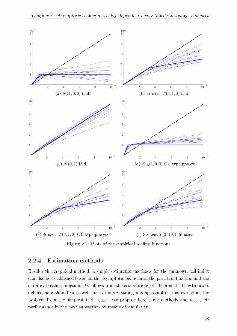
2.2.3 Plots of the empirical scaling functions
The shape of the empirical scaling function is not always ideal as its asymptotic form.
However, most plots are very close to their theoretical form. To illustrate this, we sim-
ulate 10 independent samples of size 1000 in six dierent settings. The rst three cases
studied are i.i.d. samples and others are stationary and weakly dependent, in accordance
with the assumptions of Theorem 1. Figure 2.2 summarizes the plots of the empirical
scaling functions (dotted) together with the corresponding asymptotic form (solid) and
the baseline (dot-dashed). Here, si, i = 1, . . . , N in (1.5) are chosen equidistantly in the
25

Chapter 2. Asymptotic scaling of weakly dependent heavy-tailed stationary sequences
interval [0.1, 0.9] with N = 23. The scaling function is estimated at the points qj chosen
in the interval [0, 10] with step 0.1.
The rst group of samples is generated from a stable distribution with stable index
equal to 1. A random variable Y has an α-stable distribution with index of stability α ∈(0, 2), scale parameter σ ∈ (0,∞), skewness parameter β ∈ [−1, 1] and shift parameter
µ ∈ R, denoted by Y ∼ Sα(σ, β, µ) if its characteristic function has the following form
E[eiζY
]=
exp−σα|ζ|α
(1− iβ sign(ζ) tan πα
2
)+ iζµ
, if α = 1,
exp−σ|ζ|
(1 + iβ 2
πsign(ζ) ln |ζ|
)+ iζµ
, if α = 1,
ζ ∈ R. (2.15)
If µ = 0 and α = 1, or if β = 0 and α = 1, then Y is said to have strictly stable
distribution. The second group of samples is generated from the Student t-distribution
with 3 degrees of freedom, a parameter that corresponds to the tail index. Recall that
the probability density function of the Student t-distribution T (ν, σ, µ) is
fT (ν,σ,µ)(x) =Γ(ν+1
2)
√νσ
√πΓ(ν
2)
(1 +
1
ν
(x− µ
σ
)2)− ν+1
2
, x ∈ R, (2.16)
where σ > 0 is the scale parameter, ν the tail parameter (usually called degrees of freedom)
and µ ∈ R the location parameter. Figures 2.2a and 2.2b show that for both stable and
Student case the empirical scaling functions are close to their theoretical form. Both plots
are approximately bilinear and by identifying the breakpoint, one can roughly guess the
tail index value. Also, it is clear from the shape of the empirical scaling functions that the
variance is innite in the rst case and nite in the second. The third sample is generated
from a standard normal distribution. From Figure 2.2c one can surely doubt the existence
of heavy-tails in these samples since the empirical scaling functions almost coincide with
the baseline q/2. This shows that the estimated scaling functions have the potential of
providing a self-contained characterization of the tail.
Examples shown in Figures 2.2d-2.2f are based on dependent data. Dependent samples
are generated as sample paths of two types of stochastic processes: Ornstein-Uhlenbeck
(OU) type processes and diusions. Recall that a stochastic process X = X(t), t ≥ 0is said to be of OU type if it satises a stochastic dierential equation (SDE) of the form
dX(t) = −λX(t)dt+ dL(λt), t ≥ 0, (2.17)
where L = L(t), t ≥ 0 is the background driving Lévy process (BDLP) and λ > 0. We
consider strictly stationary solutions of SDE (2.17). The α-stable OU type process with
parameter λ > 0 and 0 < α < 2 is the solution of the SDE (2.17) with L being the α-
stable Lévy process. Since the distribution of increments for the BDLP L is known in this
case, we use Euler's scheme of simulation by replacing dierentials in Equation (2.17) with
26

Chapter 2. Asymptotic scaling of weakly dependent heavy-tailed stationary sequences
dierences. Student OU type process has been introduced in Heyde & Leonenko (2005). It
can be shown that for arbitrary λ > 0 there exists a strictly stationary stochastic process
X = X(t), t ≥ 0, which has a marginal distribution T (ν, σ, µ) with density function
(2.16) and BDLP L such that (2.17) holds. This stationary process X is referred to as
the Student OU type process. Moreover, the cumulant transform of the BDLP L can be
expressed as
κL1(ζ) = logE[eiζL1
]= iζµ−
√νσ|ζ|
Kν/2−1(√νσ|ζ|)
Kν/2(√νσ|ζ|)
, ζ ∈ R, ζ = 0,
where K is the modied Bessel function of the third kind and κL1(0) = 0 (Heyde &
Leonenko (2005)). Since for the Student OU process the exact law of the increments of
the BDLP is unknown, we use the approach introduced in Taufer & Leonenko (2009) to
simulate Student OU process. This approach circumvents the problem of simulating the
jumps of the BDLP and is easily applicable when an explicit expression of the cumulant
transform is available. Both OU processes considered can be shown to posses strong
mixing property with an exponentially decaying rate (see Masuda (2004)).
The last process considered is a stationary Student diusion. In order to dene the
Student diusion, we introduce the SDE:
dX(t) = −θ (X(t)− µ) dt+
√√√√ 2θσ2
ν − 1
(ν +
(X(t)− µ
σ
)2)dB(t), t ≥ 0, (2.18)
where ν > 2, σ > 0, µ ∈ R, θ > 0, and B = B(t), t ≥ 0 is a standard Brownian motion
(BM) (see Bibby et al. (2005) and Heyde & Leonenko (2005)). The SDE (2.18) admits a
unique ergodic Markovian weak solution X = X(t), t ≥ 0, which is a diusion process
with the Student invariant distribution given by probability density function (2.16). The
diusion process which solves the SDE (2.18) is called the Student diusion. If X(0) =d
T (ν, σ, µ), the Student diusion is strictly stationary. According to Leonenko & uvak
(2010), the Student diusion is a strong mixing process with an exponentially decaying
rate. For the simulation of paths of the Student diusion process with known values of
parameters, we have used the Milstein scheme (for details see Iacus (2008)). Both OU
processes were generated with autoregression parameter λ = 1 and diusion was generated
with θ = 2.
From the examples on dependent data we can conclude that the shape of the empir-
ical scaling function is not aected with this weak form of dependence present. Again,
empirical scaling functions are very near their asymptotic form.
27
Chapter 2. Asymptotic scaling of weakly dependent heavy-tailed stationary sequences
2 4 6 8 10q
1
2
3
4
5ΤHqL
(a) S1(1, 0, 0) i.i.d.
2 4 6 8 10q
1
2
3
4
5ΤHqL
(b) Student T (3, 1, 0) i.i.d.
2 4 6 8 10q
1
2
3
4
5ΤHqL
(c) N (0, 1) i.i.d.
2 4 6 8 10q
1
2
3
4
5ΤHqL
(d) S0.5(1, 0, 0) OU type process
2 4 6 8 10q
1
2
3
4
5ΤHqL
(e) Student T (3, 1, 0) OU type process
2 4 6 8 10q
1
2
3
4
5ΤHqL
(f) Student T (3, 1, 0) diusion
Figure 2.2: Plots of the empirical scaling functions
2.2.4 Estimation methods
Besides the graphical method, a simple estimation methods for the unknown tail index
can also be established based on the asymptotic behavior of the partition function and the
empirical scaling function. As follows from the assumptions of Theorem 1, the estimators
dened here should work well for stationary strong mixing samples, thus extending the
problem from the simplest i.i.d. case. We propose here three methods and test their
performance in the next subsection by means of simulation.
28

Chapter 2. Asymptotic scaling of weakly dependent heavy-tailed stationary sequences
The basic idea of a method M1 is to estimate α by tting the empirical scaling
function to the asymptotic form τ∞α . This is done by the ordinary least squares method.
First we x some points si ∈ (0, 1), i = 1 . . . , N in the denition of the empirical scaling
function. For example, in simulations below we take equidistant points in the interval
[0.1, 0.9] with N = 23. Now, for points qi ∈ (0, qmax), i = 1, . . . ,M , we can calculate
τi = τN,n(qi) using Equation (1.5). The estimator is dened as
α1 = argminα∈(0,∞)
M∑i=1
(τi − τ∞α (qi))2. (2.19)
For practical reasons, due to complexity of the expression for τ∞α , the method is divided
into two cases: α ≤ 2 and α > 2; i.e., the corresponding part of τ∞α is used as a model
function in (2.19), depending where the true value of α is. Therefore, it is necessary to rst
detect whether we are in the case of innite variance or not. This can be accomplished
by using the graphical method described earlier. In the inconclusive case, it is advisable
to compute both estimates and compare the quality of the t. For simulations, points qiare chosen equidistantly in the interval [0, 8] with step 0.1.
If α ≤ 2, the information on α in the asymptotic form of the empirical scaling function
is hidden in the slope of the rst part and the breakpoint. When α > 2, the information
on α appears in the breakpoint and in the complicated nonlinear expression of the second
part. Method M1 tries to use all three parts in estimating α. Alternatively, we can base the
method only on a breakpoint. Since the shape of τ∞α is bilinear or approximately bilinear,
we denemethod M2 by tting the following general continuous bilinear function to the
empirical scaling function
ς(q) =
aq, if 0 < q ≤ b,
cq + b(a− c), if q > b.(2.20)
The parameter of interest is b which corresponds to a breakpoint α and the estimator by
method M2, α2, is dened as
(a, α2, c) = argmin(a,b,c)∈(0,∞)×(0,∞)×R
M∑i=1
(τi − ς(qi))2. (2.21)
This method has the advantage of not depending on whether α ≤ 2 or α > 2. More-
over, the second part depends on the rate of divergence of innite moments and may not
precisely follow the shape of τ∞α on nite samples. This part is, however, usually approxi-
mately linear and tting (2.20) makes the method more robust on the discrepancies from
τ∞α .
For the third method, we go one step back to the asymptotic behavior of the parti-
29

Chapter 2. Asymptotic scaling of weakly dependent heavy-tailed stationary sequences
tion function. As already discussed, results of Theorem 1 motivate viewing (2.3) as the
regression model. It makes sense then to estimate α from a bivariate nonlinear regression
of lnSq(n, ns)/ lnn on q and s with model function Rα(q, s). However, this complicated
regression model may not always give good results and that is why we approach it in two
steps. When dening the empirical scaling function we xed q and rst considered s as
the variable in regression, while for the third method we go the other way around.
For the moment let us x s ∈ (0, 1). The limit Rα(q, s) in Theorem 1 has the following
form for α ≤ 2:
Rα(q, s) =
sαq, if q ≤ α,
1αq + s− 1, if q > α,
(2.22)
and if α > 2 the limit is
Rα(q, s) =
s2q, if q ≤ α,
max
1αq + s− 1, s
2q, if q > α.
Notice that in this case bilinear function q 7→ max
1αq + (s− 1), s
2qhas a breakpoint at
q =s− 1s2− 1
α
.
If s ∈ (2/α, 1), q < 0 and there is no breakpoint in the range of positive q values. If
s ∈ (0, 2/α), we can write for the case α > 2:
Rα(q, s) =
s2q, if q ≤ q,
1αq + (s− 1), if q > q.
(2.23)
So, if s ∈ (0, 2/α), q 7→ Rα(q, s) is bilinear continuous and, motivated by the regression
model (2.3), we can t function (2.20) to points(qi,
lnSqi(n, ns)
lnn
): i = 1, . . . ,M
. (2.24)
This way we nd the estimated parameters of (2.20)
(as, bs, cs) = argmin(a,b,c)∈(0,∞)×(0,∞)×R
M∑i=1
(lnSqi(n, n
s)
lnn− ς(qi)
)2
.
In order to dene a method that does not depend on α ≤ 2 or not, we notice that, if
s ∈ (0, 2/α), the common part of (2.22) and (2.23) giving information on α is the slope
of the second part. Therefore, 1/cs is an estimate for α for each s ∈ (0, 2/α). Since
we do not consider problems with tail index greater than, say 8, s can be chosen in the
30

Chapter 2. Asymptotic scaling of weakly dependent heavy-tailed stationary sequences
interval (0, 0.25). We dene a method M3 estimator by averaging over a set of values
sj ∈ (0, 0.25), j = 1, . . . , N :
α3 =1
N
N∑i=1
1
csi. (2.25)
In simulations and examples below we take sj equidistantly in the interval [0.01, 0.25]
with step 0.02.
To make the estimation process by this method more clear, we illustrate it on a simple
example with data consisting of 1000 points generated from the Student t distribution
T (3, 1, 0) (Figure 2.3). Figures 2.3a-2.3e show sets of points (2.24) for dierent s values,
together with the tted bilinear function (2.20). The reciprocal of the slope of the second
part corresponds to the tail index α. These values for a range of s are shown in Figure
2.3f. By averaging, we obtain the nal estimate by method M3 to be 2.942.
Although method M3 may seem promising, it has a serious drawback of not being scale
invariant. Indeed, scaling the data by some factor c would scale the partition function by
a factor |c|q. As the samples are nite, this produces an additional term ln |c|q/ lnn in the
ordinate of the set of points (2.24) that aects the estimation process. This makes the
practical use of the method very limited. Nonetheless, we will include it in the simulation
study below in which the generated data will be chosen from distributions with scale
parameter equal to 1. These problems do not appear for the methods based on the
empirical scaling functions. Scaling functions are robust to scale change as they are based
only on the slope obtained for a xed value of q.
31

Chapter 2. Asymptotic scaling of weakly dependent heavy-tailed stationary sequences
2 4 6 8 10q
0.5
1.0
1.5
2.0
2.5
s 0.01
(a) s = 0.01
2 4 6 8 10q
0.5
1.0
1.5
2.0
2.5
s 0.07
(b) s = 0.07
2 4 6 8 10q
0.5
1.0
1.5
2.0
2.5
s 0.13
(c) s = 0.13
2 4 6 8 10q
0.5
1.0
1.5
2.0
2.5
s 0.19
(d) s = 0.19
2 4 6 8 10q
0.5
1.0
1.5
2.0
2.5
s 0.25
(e) s = 0.25
0.01 0.03 0.05 0.07 0.09 0.11 0.13 0.15 0.17 0.19 0.21 0.23 0.25s
1.5
2.0
2.5
3.0
3.5
4.0Α`
3
(f) Estimates for a range of s values
Figure 2.3: Estimation process by method M3 on Student T (3, 1, 0) data
2.2.5 Simulation study
In this subsection we provide a simulation study in order to investigate nite sample
properties of the estimators dened in the previous subsection. We choose to generate
i.i.d. random samples from the following distributions: stable distribution Sα(1, 0, 0)
with α = 0.5 and α = 1.5, Student t-distribution T (α, 1, 0) with α = 0.5, 1.5, 2.5, 3, 4 and
Pareto distribution with tail index α = 0.5, 1, 1.5 and scale parameter 1. Recall that the
32

Chapter 2. Asymptotic scaling of weakly dependent heavy-tailed stationary sequences
random variable X has Pareto distribution if its tail distribution is given by
P (X > x) =
(xm
x
)α, x ≥ xm,
1, x < xm,
where xm > 0 is the minimal possible value (scale parameter) and α > 0 is the tail index.
For each distribution we have generated 250 samples of length 1000 and computed the
estimators (2.19), (2.21) and (2.25). In addition to i.i.d. samples, we have generated
samples from stable and Student OU type process and Student diusion, in the same way
as it was done in Subsection 2.2.3.
In order to give a picture of the performance of the estimators, we compare them with
the Hill estimator. Since the Hill estimator depends on the number of order statistics k,
we do this in the following manner. For each sample we compute the value of the Hill
estimator for each k in the range 1, . . . , 250. After this is done for all 250 samples, we
choose k such that the mean square error (MSE) is minimal. So this is the smallest MSE
that can be achieved with the Hill estimator on the generated samples if k is xed for
each distribution. It is clear that this comparison is unfair to the estimators proposed in
Subsection 2.2.4, as in practice one can hardly choose an optimal k for the Hill estimator.
We note that besides the Hill estimator, we computed in the same way the moment
estimator and the Pickands estimator. However, as neither of these is signicantly better
than the Hill estimator, we do not report their results in the following.
Table 2.1: Bias (α− α) of the estimators based on 250 samples of length 1000
distribution α M1 M2 M3 Hill optimal kstable 0.5 0.1252 0.1085 0.0126 -0.0218 98stable 1.5 0.1533 0.3352 0.2914 -0.0275 211Student 0.5 0.1182 0.1194 0.0276 -0.0065 238Student 1.5 0.0716 0.1607 0.0834 -0.0938 94Student 2.5 0.5669 -0.1396 0.0025 -0.2375 44Student 3 0.3432 -0.4268 -0.1053 -0.4241 39Student 4 -0.1861 -1.1929 -0.4638 -0.6033 20Pareto 0.5 0.0654 0.1204 -0.0048 0.0011 250Pareto 1 -0.1391 0.2349 0.0003 0.0023 250Pareto 1.5 0.1736 0.1449 0.0381 0.0034 250
stable OU 0.5 0.1805 0.1965 0.0876 -0.0289 159stable OU 1.5 0.0846 0.3940 0.3113 -0.0161 209Student OU 3 1.1333 -0.4035 0.9498 -0.3224 32Student OU 4 0.4769 -1.2158 1.3796 -0.6695 23Student di 3 0.0073 -0.9425 -0.4411 -0.8703 31Student di 4 -0.5066 -1.6429 -0.5128 -1.0137 14
Table 2.1 reports the estimated bias as well as the optimal k for the Hill estimator,
while Table 2.2 shows the root of the mean square error (RMSE). Bold values show the
33

Chapter 2. Asymptotic scaling of weakly dependent heavy-tailed stationary sequences
Table 2.2: RMSE of the estimators based on 250 samples of length 1000
distribution α M1 M2 M3 Hillstable 0.5 0.2474 0.1602 0.0861 0.0504
stable 1.5 0.3027 0.4654 0.4549 0.1001
Student 0.5 0.2039 0.1606 0.0869 0.0307
Student 1.5 0.2708 0.2897 0.2783 0.1652
Student 2.5 0.9884 0.2894 0.4030 0.3950Student 3 1.0232 0.4913 0.4556 0.5704Student 4 1.3163 1.2171 0.6687 0.9418Pareto 0.5 0.1098 0.1673 0.0754 0.0316
Pareto 1 0.1470 0.3387 0.1565 0.0632
Pareto 1.5 0.3352 0.2906 0.2628 0.0948
stable OU 0.5 0.2778 0.2386 0.1389 0.0668
stable OU 1.5 0.2563 0.5112 0.4752 0.1203
Student OU 3 1.9149 0.4612 1.1514 0.5337Student OU 4 1.7082 1.2410 1.7274 0.9081
Student di 3 0.5985 0.9810 0.6821 0.9757Student di 4 1.1394 1.6655 0.9150 1.3743
best value for each case considered.
First, if we compare the three proposed methods, one can notice that method M2 is
outperformed by M1 and M3 by bias, while there is no much dierence when it comes to
RMSE. The methods M1 and M3 have similar performance with M3 slightly better when
RMSE is considered. The disadvantage of method M1 is that it depends on the knowledge
of whether α ≤ 2 or α > 2 and in some cases the estimated value may depend on the
choice of the maximal q value taken into consideration. On the other hand, method M3 is
not scale invariant which makes it less suitable for the practical examples. To summarize
these arguments, in a general situation a method M1 is recommended to use.
When compared by the RMSE, the Hill estimator shows smaller variability than the
other three estimators, especially for smaller values of α, while for larger α the proposed
methods give better results. However, one should notice that the dierences are not
substantial. Moreover, the Hill estimator's performance is reported for the optimal choice
of k, which may not be achieved in practice. On the other hand, computation of the
proposed estimators is straightforward and does not require choosing extra parameters.
If we take this in mind, the new methods can be seen as a good alternative to Hill
estimator. The comparison of method M1 and the Hill estimator is also shown by boxplots
in Figure 2.4. We illustrate more advantages of the estimator M1 on examples in the next
subsection.
34

Chapter 2. Asymptotic scaling of weakly dependent heavy-tailed stationary sequences
stableH0.5L stableH1.5L ParetoH0.5L ParetoH1L ParetoH1.5L
-0.5
0.0
0.5
1.0
1.5
M1
Hill
(a) Stable and Pareto distribution
StudentH0.5L StudentH1.5L StudentH2.5L StudentH3L StudentH4L
-2
0
2
4
6
M1
Hill
(b) Student distribution
stableOUH0.5L stableOUH1.5L StudentOUH3L StudentOUH4LStudentdiff H3LStudentdiff H4L
-2
0
2
4
M1
Hill
(c) Dependent samples
Figure 2.4: Boxplots of α− α for α1 and αHill
35

Chapter 2. Asymptotic scaling of weakly dependent heavy-tailed stationary sequences
2.2.6 Examples and comparison
In this subsection we provide several examples to illustrate how the proposed methods
work and compare them with the existing methods.
Example 1 - non heavy-tailed data
With this example we try to illustrate the potential of the empirical scaling functions as
a graphical method that can distinguish between heavy-tailed and light-tailed scenario.
Dierent methods are tested on a random sample from standard normal distribution of
size 2000. The results are shown in Figure 2.5. QQ plot for 500 largest data points
exhibits nonlinearity, thus indicating that Pareto type tail is not a good t for the data
(Figure 2.5a). For the purpose of tail analysis we plot the extreme value index (1/α)
values estimated by the moment estimator. From Figure 2.5b one can see that the plot
stabilizes at a negative value near zero. This is an indication of light tails. The scaling
function shown in Figure 2.5c is completely in accordance with this analysis. Indeed, it
almost coincides with the baseline that corresponds to a non heavy-tailed data.
1 2 3 4-log
i
k + 1
0.5
1.0
logHXiL
(a) QQ plot (k = 500)
200 400 600 800 1000k
-2.5
-2.0
-1.5
-1.0
-0.5
1
Α
(b) Moment estimator plot
2 4 6 8 10q
1
2
3
4
5
ΤHqL
(c) Empirical scaling function
Figure 2.5: Example 1 - non heavy-tailed data
36

Chapter 2. Asymptotic scaling of weakly dependent heavy-tailed stationary sequences
Example 2 - Danish re insurance claims
The second example is a practical one. The data we analyze are the Danish re insurance
claims in the period from 1980 to 1990. There are 2167 observations and the amounts
are in millions of Danish Kroner.1 The same example has been considered in (Embrechts
et al. 1997, Example 6.2.9) and in (Resnick 2007, Fig. 1.6., 4.5., 4.7.). The analysis made
in Resnick (2007) suggests that the data exhibits heavy-tails and the tail index estimate is
around 1.4 (see (Resnick 2007, Fig. 4.5.)). Hill and moment estimator plots (Figures 2.6a
and 2.6b) conrm the index value is around 1.5. The empirical scaling function, together
with the baseline, is shown in Figure 2.6c. Mean has been subtracted from the data to
adjust to the assumptions of Theorem 1. The scaling function is approximately bilinear:
the rst part of the plot has a slope greater than the baseline and the second part is
nearly horizontal. This points out that the variance is innite. The breakpoint occurs at
around 1.5, which indicates a possible value of the tail index. Estimation by method M1
gives α1 = 1.419, which is consistent with the previous analysis done in Resnick (2007).
0 200 400 600 800 1000 1200 1400k
1.0
1.5
2.0
2.5Α`
kHill
(a) Hill plot
0 200 400 600 800 1000 1200 1400k
1.0
1.5
2.0
2.5Α`
kM
(b) Moment estimator plot
2 4 6 8 10q
1
2
3
4
5
ΤHqL
(c) Empirical scaling function
Figure 2.6: Example 2 - Danish re insurance claims
1The data can be obtained from: http://www.ma.hw.ac.uk/~mcneil/data.html
37

Chapter 2. Asymptotic scaling of weakly dependent heavy-tailed stationary sequences
Example 3 - departure from Pareto tail
The Hill estimator, as well as many others, is known to behave poorly if the slowly
varying function in the tail is far away from a constant. We compare this behavior with
the performance of the empirical scaling functions on the same samples. Consider two
distribution F1, F2 dened by their tail distribution functions
F 1(x) = 1− F1(x) =1
x12
, x ≥ 1, (2.26)
F 2(x) = 1− F2(x) =e
12
x12 lnx
, x ≥ e. (2.27)
Both distributions are heavy-tailed with tail index equal to 1/2. We generate samples
from these two distributions with 5000 observations. The corresponding Hill plots are
shown in Figure 2.7a. While for the Pareto distribution F1 the Hill plot provides very
good results, for F2 it is impossible to draw any conclusion about the value of the tail
index. The plot fails to stabilize at some value and produces a departure from the true
index value. This is sometimes called the Hill horror plot (see Embrechts et al. (1997)).
The result is similar with the moment estimator: a non-constant slowly varying function
in the tail produces a signicant bias, as shown in Figure 2.7b.
0 1000 2000 3000 4000k
0.4
0.5
0.6
0.7
0.8
0.9
1.0Α
Α 0.5
Α`
kHill- F2
Α`
kHill- F1
(a) Hill plot
1000 2000 3000 4000k
0.4
0.5
0.6
0.7
0.8
0.9
1.0Α
Α 0.5
Α`
kM- F2
Α`
kM- F1
(b) Moment estimator plot
2 4 6 8 10q
1
2
3
4
5
ΤHqL
q
2
ΤΑ
¥HqL
Τ`HqL - F2
Τ`HqL - F1
(c) Scaling functions
Figure 2.7: Example 3 - departure from Pareto tail
38

Chapter 2. Asymptotic scaling of weakly dependent heavy-tailed stationary sequences
Figure 2.7c shows the empirical scaling functions for the same samples, together with
the theoretical one and the baseline. One can see that the empirical scaling functions are
very close to their asymptotic shape, especially in the rst part of the plot, before the
breakpoint. It seems that nonconstant slowly varying function aects the estimation but
the eect is not so dramatic as for the standard estimators. Calculating estimates using
method M1 yields α1 = 0.645 for F1 and α1 = 0.72 for F2.
39

Chapter 3
Asymptotic scaling of the linear
fractional stable noise
In the previous chapter, we have analyzed asymptotic properties of the partition function
for weakly dependent heavy-tailed sequences. In this chapter we do this for the linear
fractional stable noise, which is an example of a self-similar stationary sequence exhibiting
both strong dependence and heavy-tails.
We start with the denition and basic properties of the linear fractional stable motion
and then establish asymptotic behavior of the partition function and the empirical scaling
function. These results are used to dene estimation methods for the parameters of the
process. The methods are tested by simulations and on some real data examples.
3.1 Linear fractional stable motion
Empirical time series which appear in many applications display both the Joseph and
Noah eects, as coined by Mandelbrot after the biblical gures of Joseph and Noah (see
e.g. Mandelbrot (1997)). While the Joseph eect refers to long-range dependence of the
increments, the Noah eect refers to their high variability, as expressed by the power law
tails of the marginal distributions. Fractional Brownian motion (FBM) is an example of
a process exhibiting only the Joseph eect: its increments are long-range dependent but
with normal marginal distribution. On the other hand, the α-stable Lévy process with
0 < α < 2 exhibits only the Noah eect: it has independent but heavy-tailed increments
with tail index equal to α.
An example of a stochastic process which exhibits both eects is the linear fractional
stable motion (LFSM). LFSM can be dened through the stochastic integral
X(t) =1
CH,α
∫R
((t− u)
H−1/α+ − (−u)
H−1/α+
)M(du), t ∈ R, (3.1)
40

Chapter 3. Asymptotic scaling of the linear fractional stable noise
where α ∈ (0, 2), 0 < H < 1, (x)+ = max(x, 0) and where M is a random noise. More
specically, M is an α-stable random measure on R with Lebesgue control measure λ and
skewness β. This means, rst, that M is a σ-additive mapping from E = A ∈ B(R) :
λ(A) < ∞ to the space of random variables and that it is independently scattered: if
A1, A2 ∈ E are disjoint sets, then M(A1) and M(A2) are independent random variables.
Secondly, for all sets A ∈ E , M(A) has an α-stable distribution with scale parameter
λ(A)1/α and skewness parameter β, i.e. M(A) ∼ Sα(λ(A)1/α, β, 0). If α = 1 we assume
β = 0, but for other values of α,M is allowed to be skewed. Recall that stable distributions
Sα(σ, β, µ) were dened in (2.15).
If the constant CH,α in the representation (3.1) is chosen such that the scaling param-
eter of X(1) equals 1, i.e.
CH,α =
(∫R
∣∣∣(1− u)H−1/α+ − (−u)
H−1/α+
∣∣∣α du)1/α
,
then the process is called standard LFSM. The stationary sequence Yi = X(i)−X(i− 1),
i ∈ N is referred to as the linear fractional stable noise (LFSN). The LFSM process
X(t) is H-self-similar with stationary increments (see (Samorodnitsky & Taqqu 1994,
Proposition 7.4.2)). For each t, X(t) has a strictly stable distribution with stable index
α (Samorodnitsky & Taqqu 1994, Proposition 7.4.3). The parameter α governs the tail
behavior of the marginal distributions in the sense that for each t, X(t) is heavy-tailed
with tail index α, i.e. P (|X(t)| > x) = L(x)x−α where L is a slowly varying function,
more precisely, L is constant at innity. In particular, we have that E|X(t)|q = ∞ for
q ≥ α. More details on the LFSM and its properties can be found in the monograph
Samorodnitsky & Taqqu (1994).
Setting α = 2 in (3.1) reduces the LFSM to the FBM. Dependence structure of the
FBM BH(t), t ≥ 0 can be described using autocovariance function γ(h) = EY1Yh+1,
where Yi = BH(i) − BH(i − 1), i ∈ N. It can be shown that γ(h) ∼ H(2H − 1)h2H−2
as h → ∞. This implies that∑∞
h=1 γ(h) = ∞ for 1/2 < H < 1, which is a property
known as the long-range dependence. The case 0 < H < 1/2 is referred to as the negative
dependence, since the coecient H(2H − 1) is negative in this case. As the second
moment of the LFSM is innite, dependence cannot be characterized with the covariance
function. For stable processes this can be done using codierences (Samorodnitsky &
Taqqu (1994)), but there are also many other competing approaches (see e.g. Magdziarz
(2009)). Nevertheless, by analogy to the FBM, the case of LFSM with H > 1/α is referred
to as a long-range dependence and the case H < 1/α as negative dependence.
41

Chapter 3. Asymptotic scaling of the linear fractional stable noise
3.2 Asymptotic scaling
Suppose X(t), t ≥ 0 is LFSM that is sampled in a regularly spaced time instants,
X(δ), X(2δ), . . . , X(nδ). For simplicity of notation, we assume δ = 1, so we have a
sample X1, . . . , Xn. We denote by Yi = Xi − Xi−1, i ∈ N the corresponding LFSN.
Partition function can now be written as
Sq(n, t) =1
⌊n/t⌋
⌊n/t⌋∑i=1
∣∣∣∣∣∣⌊t⌋∑j=1
Y(i−1)⌊t⌋+j
∣∣∣∣∣∣q
=1
⌊n/t⌋
⌊n/t⌋∑i=1
∣∣Xi⌊t⌋ −X(i−1)⌊t⌋∣∣q ,
where q ∈ R and 1 ≤ t ≤ n. Asymptotic properties of Sq(n, t) for LFSM have been
considered in the context of multifractality detection in Heyde & Sly (2008). We go over
the methodology of the previous chapter to establish the asymptotic properties. Although
dependence restricts many of the arguments used in the previous chapter, self-similarity
simplies the proofs at many points.
In our analysis we will also include a range of negative q values. Although this may
seem unusual, nite negative order moments provide additional information on the value
of the Hurst parameter H. In particular, for q ∈ (−1, 0), stable-distributed random
variables have nite q-th absolute moment, since their probability density function is
bounded (see e.g. Zolotarev (1986)).
The main argument in establishing asymptotic properties of the partition function is
based on the following lemma. A similar result has been proved in Heyde & Sly (2008),
yet we prove it here by much simpler arguments.
Lemma 2. Suppose (Yi, i ∈ N) is a LFSN. Then for q > α,
ln (∑n
i=1 |Yi|q)lnn
P→ q
α,
as n → ∞.
Proof. Let ε > 0. Suppose δ < ε/(q − α) and dene
Zi,n = Yi 1(|Yi| ≤ n
1α+δ), i = 1, . . . , n, n ∈ N.
It follows from Karamata's theorem (Resnick (2007)) that for arbitrary r > α
E|Zi,n|r =∫ ∞
0
P (|Zi,n|r > x)dx =
∫ nr( 1α+δ)
0
P (|Yi|r > x)dx
=
∫ nr( 1α+δ)
0
L(x1r )x−α
r dx ≤ C1L(n1α+δ)nr( 1
α+δ)(−α
r+1) = C1L(n
1α+δ)n
rα−1+δ(r−α)
(3.2)
42

Chapter 3. Asymptotic scaling of the linear fractional stable noise
Next, notice that
P
(max
i=1,...,n|Yi| > n
1α+δ
)≤
n∑i=1
P(|Yi| > n
1α+δ)≤ C2n
L(n1α+δ)
(n1α+δ)α
≤ C2L(n
1α+δ)
nαδ.
Now by partitioning on the event
Yi = Zi,n, i = 1, . . . , n =Yi ≤ n
1α+δ, i = 1, . . . , n
=
max
i=1,...,n|Yi| ≤ n
1α+δ
,
using Markov's inequality and (3.2) we have
P
(ln (∑n
i=1 |Yi|q)lnn
>q
α+ ε
)= P
(n∑
i=1
|Yi|q > nqα+ε
)
≤ P
(n∑
i=1
|Yi|q > nqα+ε, max
i=1,...,n|Yi| ≤ n
1α+δ
)+ P
(max
i=1,...,n|Yi| > n
1α+δ
)
≤ P
(n∑
i=1
|Zi,n|q > nqα+ε
)+ P
(max
i=1,...,n|Yi| > n
1α+δ
)≤ nE |Zi,n|q
nqα+ε
+ C2L(n
1α+δ)
nαδ
≤ n
nqα+ε
C1L(n1α+δ)n
qα−1+δ(q−α)) + C2
L(n1α+δ)
nαδ≤ C1L(n
1α+δ)nδ(q−α)−ε + C2
L(n1α+δ)
nαδ→ 0,
as n → ∞, since δ(q−α)−ε < 0 and L(x) is slowly varying, thus bounded by any positive
power of x, as x → ∞.
For the reverse inequality notice that since Yi is a stationary strictly α-stable sequence
corresponding to a dissipative ow it follows by (Samorodnitsky 2004, Theorem 4.8) that
maxi=1,...,n |Yi|/n1/α converges in distribution to some positive random variable. So for
any δ > 0
P
(max
i=1,...,n|Yi| < n
1α−δ
)→ 0, as n → ∞.
Now it follows that
P
(ln (∑n
i=1 |Yi|q)lnn
<q
α− ε
)= P
(n∑
i=1
|Yi|q < nqα−ε
)≤ P
(max
i=1,...,n|Yi| < n
1α− ε
q
)→ 0,
as n → ∞ which proves the statement.
Theorem 3. Suppose (Yi, i ∈ N) is a LFSN. Then for every q > −1 and every s ∈ (0, 1)
lnSq(n, ns)
lnn
P→ RH,α(q, s) :=
sqH, if q ≤ α,
s(1 + qH − q
α
)+ q
α− 1, if q > α,
(3.3)
as n → ∞.
43

Chapter 3. Asymptotic scaling of the linear fractional stable noise
Proof. By H-self-similarity of the LFSM it follows that
Sq(n, ns)
d=
nsqH
n1−s
n1−s∑i=1
|X(i)−X(i− 1)|q = nsqH
n1−s
n1−s∑i=1
|Yi|q . (3.4)
The LFSN sequence (Yi, i ∈ N) is a stable mixed moving average, which is known to be
ergodic (see Cambanis et al. (1987), Surgailis et al. (1993) or Pipiras & Taqqu (2002)).
For q ∈ (−1, α), E|Yi|q < ∞, so it follows by the ergodic theorem that
1
n1−s
n1−s∑i=1
|Yi|q → E|X(1)|q a.s.
and in particular
ln
(nsqH
n1−s
n1−s∑i=1
|Yi|q)
− lnnsqH P→ lnE|X(1)|q.
Since
ln
(nsqH
n1−s
n1−s∑i=1
|Yi|q)
− lnnsqH d= lnn
(lnSq(n, n
s)
lnn− sqH
),
this implies the statement of the theorem for q < α.
Now we consider the case q > α. We have by (3.4) that
lnSq(n, ns)
lnn− s
(1 + qH − q
α
)−( qα− 1)
d=
(sqH − 1 + s) lnn+ ln(∑n1−s
i=1 |Yi|q)
lnn− s
(1 + qH − q
α
)−( qα− 1)
=ln(∑n1−s
i=1 |Yi|q)
lnn− q
α(1− s)
=ln(∑n1−s
i=1 |Yi|q)
lnn1−s(1− s)− q
α(1− s).
Since by Lemma 2ln(∑n1−s
i=1 |Yi|q)
lnn1−s
P→ q
α, as n → ∞,
it follows that
P
(∣∣∣∣ lnSq(n, ns)
lnn− s
(1 + qH − q
α
)−( qα− 1)∣∣∣∣ > ε
)
= P
∣∣∣∣∣∣ln(∑n1−s
i=1 |Yi|q)
lnn1−s− q
α
∣∣∣∣∣∣ (1− s) > ε
→ 0,
as n → ∞ and this proves the second case. The case q = α follows by the same argument
44

Chapter 3. Asymptotic scaling of the linear fractional stable noise
as (c) part of the proof of Theorem 1.
The previous theorem can be seen as an analogue of Theorem 1. As opposed to the
setting of the previous chapter, the limit now additionally depends on the value of the
parameter H. It is clear from (3.3) that lnSq(n, ns)/ lnn should behave approximately
linearly in s. It thus makes sense to focus on the slope of the simple linear regression of
lnSq(n, ns)/ lnn on s for a xed value of q. We now establish an analog of Theorem 2 on
the empirical scaling function.
Theorem 4. Suppose that the assumptions of Theorem 3 hold and x s1, . . . , sN in the
denition of the empirical scaling function (1.5). Then for every q > −1
τN,n(q)P→ τ∞H,α(q) :=
Hq, if q ≤ α,(H − 1
α
)q + 1, if q > α,
(3.5)
as n → ∞.
Proof. Fix q > −1 and let ε > 0, δ > 0 and
C =N∑i=1
(si)2 − 1
N
(N∑i=1
si
)2
> 0.
By Theorem 3, for each i = 1, . . . , N there exist n(1)i such that
P
(∣∣∣∣ lnSq(n, nsi)
lnn−RH,α(q, si)
∣∣∣∣ > εC
2siN
)<
δ
2N, n ≥ n
(1)i .
It follows then that for n ≥ n(1)max := maxn(1)
1 , . . . , n(1)N
P
(∣∣∣∣∣N∑i=1
silnSq(n, n
si)
lnn−
N∑i=1
siRH,α(q, si)
∣∣∣∣∣ > εC
2
)
≤ P
(N∑i=1
si
∣∣∣∣ lnSq(n, nsi)
lnn−RH,α(q, si)
∣∣∣∣ > εC
2
)
≤N∑i=1
P
(∣∣∣∣ lnSq(n, nsi)
lnn−RH,α(q, si)
∣∣∣∣ > εC
2siN
)<
δ
2.
Similarly, for each i = 1, . . . , N there exist n(2)i such that
P
∣∣∣∣ lnSq(n, nsi)
lnn−RH,α(q, si)
∣∣∣∣ > εC
2(∑N
i=1 si
) <
δ
2N, n ≥ n
(2)i ,
45

Chapter 3. Asymptotic scaling of the linear fractional stable noise
and for n ≥ n(2)max := maxn(2)
1 , . . . , n(2)N
P
(∣∣∣∣∣ 1NN∑i=1
si
N∑j=1
lnSq(n, nsj)
lnn− 1
N
N∑i=1
si
N∑j=1
RH,α(q, sj)
∣∣∣∣∣ > εC
2
)
≤ P
N∑j=1
∣∣∣∣ lnSq(n, nsj)
lnn−RH,α(q, sj)
∣∣∣∣ > NεC
2(∑N
i=1 si
)
≤N∑j=1
P
∣∣∣∣ lnSq(n, nsj)
lnn−RH,α(q, sj)
∣∣∣∣ > εC
2(∑N
i=1 si
) <
δ
2.
Finally then, for n ≥ maxn(1)max, n
(2)max it follows that
P
∣∣∣∣∣∣∣τN,n(q)−
∑Ni=1 siRH,α(q, si)− 1
N
∑Ni=1 si
∑Nj=1RH,α(q, sj)∑N
i=1 (si)2 − 1
N
(∑Ni=1 si
)2∣∣∣∣∣∣∣ > ε
≤ P
(∣∣∣∣∣N∑i=1
silnSq(n, n
si)
lnn−
N∑i=1
siRH,α(q, si)
∣∣∣∣∣+
∣∣∣∣∣ 1NN∑i=1
si
N∑j=1
lnSq(n, nsj)
lnn− 1
N
N∑i=1
si
N∑j=1
RH,α(q, sj)
∣∣∣∣∣ > εC
)
≤ P
(∣∣∣∣∣N∑i=1
silnSq(n, n
si)
lnn−
N∑i=1
siRH,α(q, si)
∣∣∣∣∣ > εC
2
)
+ P
(∣∣∣∣∣ 1NN∑i=1
si
N∑j=1
lnSq(n, nsj)
lnn− 1
N
N∑i=1
si
N∑j=1
RH,α(q, sj)
∣∣∣∣∣ > εC
2
)< δ,
and thus
τN,n(q)P→∑N
i=1 siRH,α(q, si)− 1N
∑Ni=1 si
∑Nj=1 RH,α(q, sj)∑N
i=1 (si)2 − 1
N
(∑Ni=1 si
)2 , as n → ∞.
It remains to show that the right hand side is exactly τ∞H,α(q) from (3.5). Indeed, when
q ≤ α we have ∑Ni=1 qHs2i − 1
N
∑Ni=1 si
∑Nj=1 qHsj∑N
i=1 (si)2 − 1
N
(∑Ni=1 si
)2 = Hq
46
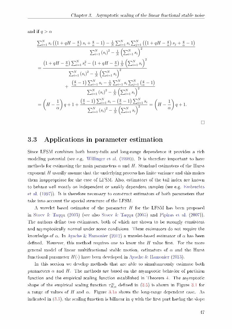
Chapter 3. Asymptotic scaling of the linear fractional stable noise
and if q > α∑Ni=1 si
((1 + qH − q
α
)si +
qα− 1)− 1
N
∑Ni=1 si
∑Nj=1
((1 + qH − q
α
)sj +
qα− 1)
∑Ni=1 (si)
2 − 1N
(∑Ni=1 si
)2=
(1 + qH − q
α
)∑Ni=1 s
2i −
(1 + qH − q
α
)1N
(∑Ni=1 si
)2∑N
i=1 (si)2 − 1
N
(∑Ni=1 si
)2+
(qα− 1)∑N
i=1 si −1N
∑Ni=1 si
∑Nj=1
(qα− 1)
∑Ni=1 (si)
2 − 1N
(∑Ni=1 si
)2=
(H − 1
α
)q + 1 +
(qα− 1)∑N
i=1 si −(qα− 1)∑N
i=1 si∑Ni=1 (si)
2 − 1N
(∑Ni=1 si
)2 =
(H − 1
α
)q + 1.
3.3 Applications in parameter estimation
Since LFSM combines both heavy-tails and long-range dependence it provides a rich
modeling potential (see e.g. Willinger et al. (1998)). It is therefore important to have
methods for estimating the main parameters α and H. Standard estimators of the Hurst
exponent H usually assume that the underlying process has nite variance and this makes
them inappropriate for the case of LFSM. Also, estimators of the tail index are known
to behave well mostly on independent or weakly dependent samples (see e.g. Embrechts
et al. (1997)). It is therefore necessary to construct estimators of both parameters that
take into account the special structure of the LFSM.
A wavelet based estimator of the parameter H for the LFSM has been proposed
in Stoev & Taqqu (2003) (see also Stoev & Taqqu (2005) and Pipiras et al. (2007)).
The authors dene two estimators, both of which are shown to be strongly consistent
and asymptotically normal under some conditions. These estimators do not require the
knowledge of α. In Ayache & Hamonier (2012) a wavelet-based estimator of α has been
dened. However, this method requires one to know the H value rst. For the more
general model of linear multifractional stable motion, estimators of α and the Hurst
functional parameter H(·) have been developed in Ayache & Hamonier (2013).
In this section we develop methods that are able to simultaneously estimate both
parameters α and H. The methods are based on the asymptotic behavior of partition
function and the empirical scaling function established in Theorem 4. The asymptotic
shape of the empirical scaling function τ∞H,α dened in (3.5) is shown in Figure 3.1 for
a range of values of H and α. Figure 3.1a shows the long-range dependent case. As
indicated in (3.5), the scaling function is bilinear in q with the rst part having the slope
47

Chapter 3. Asymptotic scaling of the linear fractional stable noise
H. A break occurs at α and the plot is linear again but now with the slope H − 1/α.
In the negative dependence case H < 1/α (Figure 3.1b), the second part has a negative
slope.
-1 1 2 3 4q
-0.5
0.5
1.0
ΤH ,Α¥ HqL
H=0.9, Α=1.2
H=0.8, Α=1.3
H=0.7, Α=1.5
H=0.6, Α=1.7
(a) Case H > 1α
-1 1 2 3 4q
-2.0
-1.5
-1.0
-0.5
0.5
ΤH ,Α¥ HqL
H=0.8, Α=0.6
H=0.6, Α=0.8
H=0.4, Α=1.1
H=0.2, Α=1.5
(b) Case H < 1α
Figure 3.1: Asymptotic scaling function τ∞H,α
Figure 3.2 shows the empirical scaling functions (dashed) for some of the H and α
values presented in Figure 3.1. Their computation is based on one sample path realization
of length 15784 (explained later). Here, and in every other example of this chapter, si,
i = 1, . . . , N in (1.4) are chosen equidistantly in the interval [0.1, 0.9] with N = 23. The
scaling function is estimated at points qj chosen equidistantly in the interval [−1, 4] with
step 0.1. On each plot in Figure 3.2 the corresponding true scaling function is shown by
a solid line. Although the break is not sharp, one can notice the bilinear shape.
48

Chapter 3. Asymptotic scaling of the linear fractional stable noise
-1 1 2 3 4q
-0.5
0.5
1.0
ΤHqL
(a) H = 0.8, α = 1.3
-1 1 2 3 4q
-0.5
0.5
1.0
ΤHqL
(b) H = 0.9, α = 1.2
-1 1 2 3 4q
-1.5
-1.0
-0.5
0.5
ΤHqL
(c) H = 0.6, α = 0.8
-1 1 2 3 4q
-1.5
-1.0
-0.5
0.5
ΤHqL
(d) H = 0.8, α = 0.6
Figure 3.2: Empirical scaling functions (dashed) with the corresponding τ∞H,α
3.3.1 Estimation methods
We now specify the estimation methods for the parameters H and α, similarly as it was
done in Subsection 2.2.4.
Let us rst mention that one method can be based on the results of Theorem 3. By
choosing points 0 ≤ s1 < · · · < sN ≤ 1 and qj ∈ (−1, qmax), j = 1, . . . ,M , based on the
sample of length n, we can calculatelnSqj(n, n
si)
lnn: i = 1, . . . , N, j = 1, . . . ,M
. (3.6)
As lnSqj(n, nsi)/ lnn is expected to behave as RH,α(qj, si) dened in (3.3), we can dene
the method MI estimator for (H,α) by minimizing the dierence between the two in
the sense of the ordinary least squares, i.e.
(H1, α1) = argmin(H,α)∈(0,1)×(0,2)
N∑i=1
M∑j=1
(lnSqj(n, n
si)
lnn−RH,α(qj, si)
)2
. (3.7)
Although this method follows naturally from Theorem 3, it has a disadvantage of being
sensitive to the scale parameter of the data similarly as method M3 of the previous
chapter. Again, scaling the data by factor c would produce an additional term ln |c|q/ lnn
49

Chapter 3. Asymptotic scaling of the linear fractional stable noise
in Equation (3.7). If the underling process is standard LFSM, then the scale parameter
equals 1 and this would not cause the problem. However, for real data this is usually not
the case. For this reason, we would not consider this method in more details, although
it will be tested by simulations in the next subsection. To avoid this issue, we specify
two other methods which are based only on the slope of RH,α and are not aected by an
underlying scale parameter.
Method MII is based on the empirical scaling function (1.4) and Theorem 4. In
contrast to MI, we proceed here in two steps. First, based on the data set (3.6) for each
qj, j = 1, . . . ,M we compute the empirical scaling function τN,n(qj) as dened in (1.4).
Since for large samples this converges to τ∞H,α(qj) for each j, we dene estimators based
on the empirical scaling function as
(H2, α2) = argmin(H,α)∈(0,1)×(0,2)
M∑j=1
(τN,n(qj)− τ∞H,α(qj)
)2. (3.8)
In simulations and examples below we choose qj, j = 1, . . . ,M equidistantly in the interval
[−1, 4] with step 0.2, in order to cover the range of α ∈ (0, 2) values.
The slope of the rst part (q < α) of the empirical scaling function corresponds to
H, the breakpoint corresponds to α and the slope of the second part (q > α) contains
information about both parameters H and α. In some examples, as well as in those in
Figure 3.2, the slope of the second part does not give the value H − 1/α very precisely,
although the rst part and the breakpoint behave as expected from (3.5). The second
part corresponds to the rate of growth under innite moments, which makes it a sensitive
quantity to measure. Moreover, it depends on both parameters H and α. This can aect
the estimation even when there is an obvious bilinear shape. For this reason we provide
an alternative estimation method which uses only the information from the rst part of
the scaling function and the breakpoint, analogues to method M2 of Subsection 2.2.4.
Method MIII ts the following general continuous bilinear function to the empirical
scaling function
ς(q) =
aq, if q ≤ b,
cq + b(a− c), if q > b.(3.9)
Here we are interested in two parameters: a which corresponds to H and b which corre-
sponds to α. The estimators by method MIII are now dened as
(H3, α3, c) = argmin(a,b,c)∈(0,1)×(0,2)×R
M∑j=1
(τN,n(qj)− ς(qj))2 . (3.10)
50

Chapter 3. Asymptotic scaling of the linear fractional stable noise
3.3.2 Simulation study
We use simulation to test the bias and variability of the estimators (3.7), (3.8) and (3.10).
We also compare the methods to see which one provides the best results.
In order to simulate paths of LFSM we have used fast Fourier transform (FFT) based
algorithm, described in Stoev & Taqqu (2004). All generated sample paths are of length
15784 and additional parameters of the generator are chosen to be m = 128 and M = 600.
This makes m(M + 15784) to be a power of 2 and the algorithm uses FFT (see Stoev &
Taqqu (2004) for more details). In all cases we use symmetric α-stable LFSM and the
scale parameter of X(1) is set to 1.
Simulations were conducted as follows. We chose for α values 0.3, 0.7, 1, 1.3, 1.7 and
for H values 0.2, 0.4, 0.6, 0.8, which makes a total of 20 cases. For each case, 100 sample
paths of length 15784 have been simulated. For each sample we compute the estimates
(H1, α1), (H2, α2) and (H3, α3) corresponding to each of the methods. The mean bias and
RMSE of each estimator have been computed for each case. The results are shown in
Table 3.1 and Table 3.2. We compare the methods by indicating the better values in bold
for each parameter separately.
Table 3.1: Bias of the estimators based on 100 sample paths
H α H1 −H H2 −H H3 −H α1 − α α2 − α α3 − α
0.2
0.3 0.1076 0.1898 0.1888 0.0199 0.0124 -0.0089
0.7 0.0349 0.0472 0.0869 0.0325 0.0317 -0.07981 0.0250 -0.0162 0.0304 0.0396 0.0958 -0.1137
1.3 0.0227 -0.0377 0.0112 0.0590 0.1854 -0.14651.7 0.0266 0.0048 0.0014 0.1640 0.2253 -0.0950
0.4
0.3 -0.0129 0.0877 0.0876 0.0243 0.0167 -0.0062
0.7 -0.0208 -0.0208 0.0138 0.0456 0.0486 -0.06321 -0.0071 -0.0590 -0.0085 0.0543 0.1222 -0.1005
1.3 0.0071 -0.0533 -0.0053 0.0707 0.1951 -0.12651.7 0.0176 0.0040 0.0024 0.1572 0.2045 -0.0870
0.6
0.3 -0.1210 -0.0240 -0.0227 0.0295 0.0242 -0.0013
0.7 -0.0650 -0.0910 -0.0515 0.0627 0.0793 -0.0442
1 -0.0234 -0.0855 -0.0277 0.0663 0.1423 -0.08281.3 0.0064 -0.0432 -0.0033 0.0579 0.1546 -0.11741.7 0.0139 -0.0022 -0.0016 0.1395 0.1899 -0.0921
0.8
0.3 -0.2230 -0.1159 -0.1156 0.0360 0.0305 0.0030
0.7 -0.1109 -0.1507 -0.1195 0.0824 0.1097 -0.0098
1 -0.0309 -0.0883 -0.0513 0.0622 0.1334 -0.0360
1.3 0.0072 -0.0379 -0.0079 0.0276 0.1126 -0.1016
1.7 -0.0176 -0.0356 -0.0466 0.1626 0.2261 -0.0382
The comparison based on the RMSE from Table 3.2 shows that method MIII provides
the best results for both parameters. Table 3.1 indicates that MI and MIII provide smaller
bias than MII, although the dierences between the estimators are not substantial. Having
51
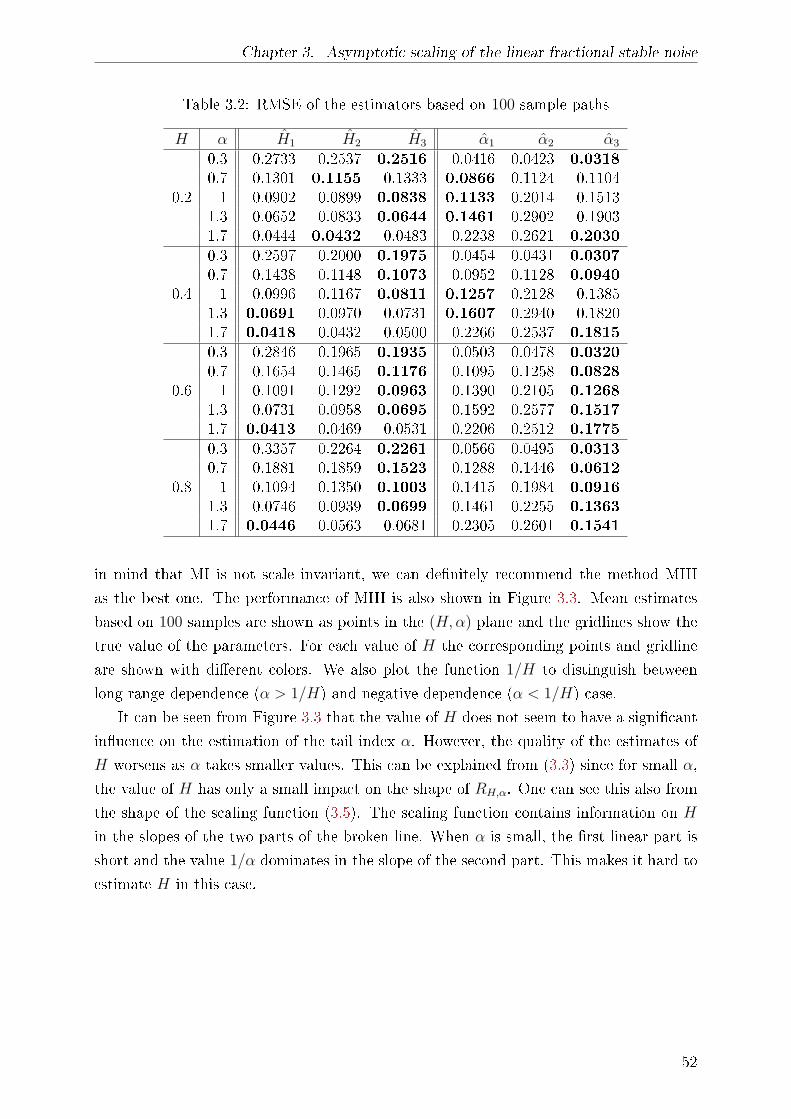
Chapter 3. Asymptotic scaling of the linear fractional stable noise
Table 3.2: RMSE of the estimators based on 100 sample paths
H α H1 H2 H3 α1 α2 α3
0.2
0.3 0.2733 0.2537 0.2516 0.0416 0.0423 0.0318
0.7 0.1301 0.1155 0.1333 0.0866 0.1124 0.11041 0.0902 0.0899 0.0838 0.1133 0.2014 0.1513
1.3 0.0652 0.0833 0.0644 0.1461 0.2902 0.19031.7 0.0444 0.0432 0.0483 0.2238 0.2621 0.2030
0.4
0.3 0.2597 0.2000 0.1975 0.0454 0.0431 0.0307
0.7 0.1438 0.1148 0.1073 0.0952 0.1128 0.0940
1 0.0996 0.1167 0.0811 0.1257 0.2128 0.13851.3 0.0691 0.0970 0.0731 0.1607 0.2940 0.18201.7 0.0418 0.0432 0.0500 0.2266 0.2537 0.1815
0.6
0.3 0.2846 0.1965 0.1935 0.0503 0.0478 0.0320
0.7 0.1654 0.1465 0.1176 0.1095 0.1258 0.0828
1 0.1091 0.1292 0.0963 0.1390 0.2105 0.1268
1.3 0.0731 0.0958 0.0695 0.1592 0.2577 0.1517
1.7 0.0413 0.0469 0.0531 0.2206 0.2512 0.1775
0.8
0.3 0.3357 0.2264 0.2261 0.0566 0.0495 0.0313
0.7 0.1881 0.1859 0.1523 0.1288 0.1446 0.0612
1 0.1094 0.1350 0.1003 0.1415 0.1984 0.0916
1.3 0.0746 0.0939 0.0699 0.1461 0.2255 0.1363
1.7 0.0446 0.0563 0.0681 0.2305 0.2601 0.1541
in mind that MI is not scale invariant, we can denitely recommend the method MIII
as the best one. The performance of MIII is also shown in Figure 3.3. Mean estimates
based on 100 samples are shown as points in the (H,α) plane and the gridlines show the
true value of the parameters. For each value of H the corresponding points and gridline
are shown with dierent colors. We also plot the function 1/H to distinguish between
long-range dependence (α > 1/H) and negative dependence (α < 1/H) case.
It can be seen from Figure 3.3 that the value of H does not seem to have a signicant
inuence on the estimation of the tail index α. However, the quality of the estimates of
H worsens as α takes smaller values. This can be explained from (3.3) since for small α,
the value of H has only a small impact on the shape of RH,α. One can see this also from
the shape of the scaling function (3.5). The scaling function contains information on H
in the slopes of the two parts of the broken line. When α is small, the rst linear part is
short and the value 1/α dominates in the slope of the second part. This makes it hard to
estimate H in this case.
52

Chapter 3. Asymptotic scaling of the linear fractional stable noise
0.2 0.4 0.6 0.8 10
0.3
0.7
1
1.3
1.7
2
H
Α
Figure 3.3: Mean estimates of (H3, α3)
All three methods can estimate both parameters H and α simultaneously. In view
of the results of Chapter 2, we nd it interesting to also study how an estimation of the
tail index would behave if the dependence structure is stronger and the parameter H
measuring dependence is known. So we included in the simulation the behavior of the
estimators MII and MIII when H is known. We also did this for the estimators of H
assuming α is known. In these cases (3.8) and (3.10) reduce to the minimization of an
univariate function.
When one of the parameters is known, both methods MII and MIII behave equally
well. Here we present only the mean estimates by method MII (Figure 3.4). The mean
estimates of α when H is known are shown in Figure 3.4a. Figure 3.4b shows a similar
plot for the estimated value of H assuming α is known. In the case of the estimation
of α (Figure 3.4a), one sees that estimators based on the scaling function, like the one
proposed in the previous chapter, can perform well even under complicated dependence
structure.
æ æ æ æ
æ æ æ æ
æ æ æ æ
æ æ æ æ
æ ææ
æ
0.2 0.4 0.6 0.8 10
0.3
0.7
1
1.3
1.7
2
H
Α`
(a) Estimates α2, H known
æ
æ
æ ææ
æ
ææ æ
æ
æ
æ æ ææ
ææ æ æ
æ
0 0.3 0.7 1 1.3 1.7 2
0.2
0.4
0.6
0.8
1
Α
H`
(b) Estimates H2, α known
Figure 3.4: Mean estimates assuming one parameter is known
53
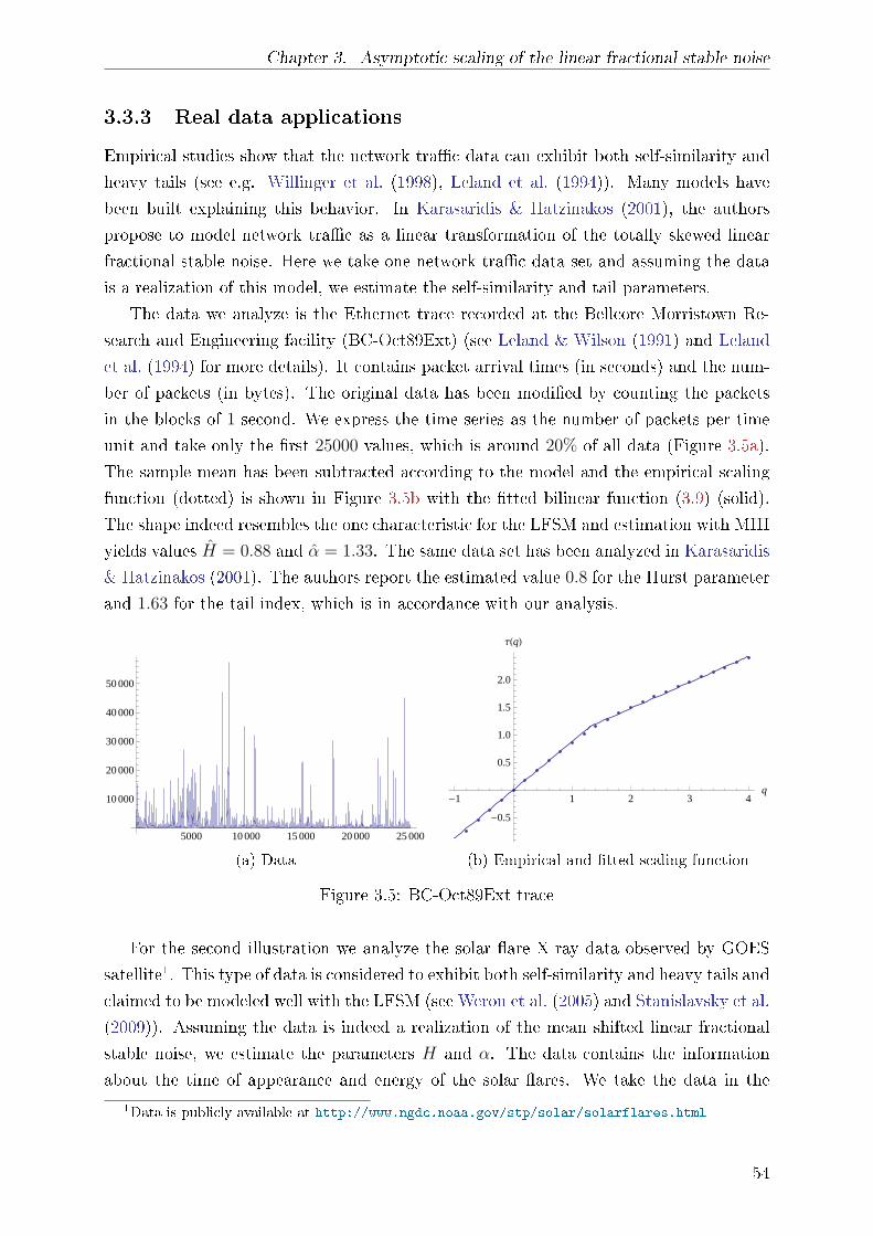
Chapter 3. Asymptotic scaling of the linear fractional stable noise
3.3.3 Real data applications
Empirical studies show that the network trac data can exhibit both self-similarity and
heavy tails (see e.g. Willinger et al. (1998), Leland et al. (1994)). Many models have
been built explaining this behavior. In Karasaridis & Hatzinakos (2001), the authors
propose to model network trac as a linear transformation of the totally skewed linear
fractional stable noise. Here we take one network trac data set and assuming the data
is a realization of this model, we estimate the self-similarity and tail parameters.
The data we analyze is the Ethernet trace recorded at the Bellcore Morristown Re-
search and Engineering facility (BC-Oct89Ext) (see Leland & Wilson (1991) and Leland
et al. (1994) for more details). It contains packet arrival times (in seconds) and the num-
ber of packets (in bytes). The original data has been modied by counting the packets
in the blocks of 1 second. We express the time series as the number of packets per time
unit and take only the rst 25000 values, which is around 20% of all data (Figure 3.5a).
The sample mean has been subtracted according to the model and the empirical scaling
function (dotted) is shown in Figure 3.5b with the tted bilinear function (3.9) (solid).
The shape indeed resembles the one characteristic for the LFSM and estimation with MIII
yields values H = 0.88 and α = 1.33. The same data set has been analyzed in Karasaridis
& Hatzinakos (2001). The authors report the estimated value 0.8 for the Hurst parameter
and 1.63 for the tail index, which is in accordance with our analysis.
5000 10 000 15 000 20 000 25 000
10 000
20 000
30 000
40 000
50 000
(a) Data
-1 1 2 3 4q
-0.5
0.5
1.0
1.5
2.0
ΤHqL
(b) Empirical and tted scaling function
Figure 3.5: BC-Oct89Ext trace
For the second illustration we analyze the solar are X-ray data observed by GOES
satellite1. This type of data is considered to exhibit both self-similarity and heavy tails and
claimed to be modeled well with the LFSM (see Weron et al. (2005) and Stanislavsky et al.
(2009)). Assuming the data is indeed a realization of the mean shifted linear fractional
stable noise, we estimate the parameters H and α. The data contains the information
about the time of appearance and energy of the solar ares. We take the data in the1Data is publicly available at http://www.ngdc.noaa.gov/stp/solar/solarflares.html
54

Chapter 3. Asymptotic scaling of the linear fractional stable noise
period from August, 1999 to December, 2003, aggregate the maximum ux values on a
daily basis and set the mean to 0, which provides 1405 data points. Figure 3.6a shows
the plot of the data and Figure 3.6b the empirical scaling function with the tted bilinear
function (3.9). The estimated values of the parameters are H = 0.75 and α = 1.56.
200 400 600 800 1000 1200 1400
0.001
0.002
0.003
0.004
(a) Data
-1 1 2 3 4q
-0.5
0.5
1.0
1.5
2.0ΤHqL
(b) Empirical and tted scaling function
Figure 3.6: Solar are X-ray data
55

Chapter 4
Detecting multifractality of time series
In this chapter we introduce the notion of a multifractal stochastic process. There is no
unique denition, so we provide an overview of dierent properties usually referred to
as multifractality. The importance of such processes is still a subject of debate, mainly
because there is no reliable statistical method that would conrm the occurrence of multi-
fractal properties in empirical time series. We make a contribution to this problem in the
second part of this chapter, where we analyze the implications of the results of Chapters
2 and 3 on one of the detection methods.
4.1 Multifractal stochastic processes
The starting point of the multifractal theory can be traced back to the work of Mandel-
brot in the context of turbulence modeling, continuing the earlier work of Kolmogorov,
Yaglom and Obukhov. In his seminal papers Mandelbrot (1972) and Mandelbrot (1974),
Mandelbrot introduced multiplicative cascades in the setting of measures, but also allow-
ing the randomness in the construction. The term multifractal was coined to refer to
cascades and is attributed to Frisch and Parisi (Frisch & Parisi (1985)). Cascades have
many interesting properties which became a model for characterizing more general ob-
jects. Geometrical properties of the sets of irregularities of cascades have led to extending
the notion of multifractality to functions and motivated studying ne scale properties of
functions (see e.g. Jaard (1996)). In this setting, multifractal analysis deals with the
local irregularities of functions characterized by the Hausdor dimension of sets of points
having the same pointwise Hölder exponent. For multifractal functions these sets are
interwoven and have noninteger Hausdor dimension. This notion can be generalized to
stochastic processes by simply applying the denition for a function on the sample paths.
On the other hand, scaling properties of cascades can be seen as a generalization
of the self-similarity. This led to a consideration of a new class of stochastic processes,
called multifractal, characterized by global scaling properties that extend self-similarity in
dierent manners. However, this can lead to discrepancy. For example, strictly α-stable
56

Chapter 4. Detecting multifractality of time series
Lévy processes with 0 < α < 2 are known to be self-similar with Hurst parameter 1/α.
On the other hand, the sample paths of these processes exhibit multifractal features (see
Jaard (1999)).
The example of cascade suggests that local irregularities are closely related with global
scaling properties. This is precisely described with the so-called multifractal formalism.
There has been an extensive research questioning when this formalism holds in dierent
settings (see Jaard (1997a,b, 2000), Riedi (1995, 2003)). Numerically, ne irregularities
are unreachable without such property. For this reason, many dierent denitions have
been introduced in order to achieve the validity of the formalism.
In this section we provide an overview of dierent scaling relations for stochastic
processes that are usually referred to as multifractality. Examples are provided illustrating
each of these properties.
4.1.1 Denitions of multifractality
The best known scaling relation in the theory of stochastic processes is self-similarity. A
stochastic process X(t), t ≥ 0 is said to be self-similar if for any a > 0, there exists
b > 0 such that
X(at) d= bX(t), (4.1)
where · d= · stands for the equality of nite dimensional distributions. A process
X(t), t ≥ 0 is said to be stochastically continuous at 0 if for every ε > 0, P (|X(h) −X(0)| > ε) → 0 as h → 0. If X(t), t ≥ 0 is self-similar, nontrivial and stochastically
continuous at 0, then b in (4.1) must be of the form aH for some H ≥ 0, i.e.
X(at) d= aHX(t). (4.2)
The proof of this fact can be found in Embrechts & Maejima (2002). These weak as-
sumptions are assumed to hold for every self-similar process considered latter on. The
exponent H is called the Hurst parameter and we say X(t), t ≥ 0 is H-ss or H-sssi if it
also has stationary increments.
Following Mandelbrot et al. (1997), the denition of a multifractal that we present
rst is motivated by generalizing the scaling rule of self-similar processes in the following
manner:
Denition 1. A stochastic process X(t) is said to be multifractal if
X(ct) d= M(c)X(t), (4.3)
where for every c > 0,M(c) is a random variable independent of X(t) whose distribution
57
Chapter 4. Detecting multifractality of time series
does not depend on t.
When M(c) is nonrandom for every c > 0, the process is self-similar and M(c) = cH
if the process is nontrivial and stochastically continuous at 0. The scaling factor M(c) is
assumed to satisfy the following property:
M(ab)d= M1(a)M2(b), (4.4)
for every choice of a and b, where M1 and M2 are independent copies of M . This general-
izes the property of the nonrandom factor for H-ss processes (ab)H = aHbH . A motivation
for this property can be found in Mandelbrot et al. (1997).
However, instead of Denition 1, scaling is usually specied in terms of moments. The
idea of extracting the scaling properties from average type quantities, like Lp norm, dates
back to the work of Frisch and Parisi (Frisch & Parisi (1985)).
Denition 2. A stochastic process X(t) is said to be multifractal if there exist functionsc(q) and τ(q) such that
E|X(t)−X(s)|q = c(q)|t− s|τ(q), ∀t, s ∈ T , ∀q ∈ Q, (4.5)
where T and Q are intervals on the real line with positive length and 0 ∈ T .
The function τ(q) is called the scaling function. Set Q can also include negative reals.
The denition can also be based on the moments of the process instead of the moments
of increments, i.e. E|X(t)| = c(q)tτ(q). If the increments are stationary, these denitions
coincide. It is clear that if X(t) is H-sssi, then τ(q) = Hq where it is dened.
The following argument shows that τ must be concave. Let q1, q2 ∈ Q, w1, w2 > 0,
w1 + w2 = 1 and q = w1q1 + w2q2. From Hölder's inequality it follows
E|X(t)−X(s)|q ≤ (E|X(t)−X(s)|q1)w1 (E|X(t)−X(s)|q2)w2 .
Taking logarithms gives
ln c(q) + τ(q) ln |t− s| ≤ (w1τ(q1) + w2τ(q2)) ln |t− s|+ (w1 ln c(q1) + w2 ln c(q2)) .
Dividing by ln |t−s| < 0 and letting t → s gives τ(q) ≥ w1τ(q1)+w2τ(q2), so τ is concave.
If T = [0,∞), then by letting t → ∞ we would get the opposite inequality τ(q) ≤w1τ(q1) + w2τ(q2), showing τ is linear. Therefore, strict concavity can hold only over a
nite time horizon, otherwise τ(q) would be linear. This is not considered to be a problem
for practical purposes (see Mandelbrot et al. (1997) for details). Since the scaling function
is linear for self-similar processes, every departure from linearity can be attributed to
58

Chapter 4. Detecting multifractality of time series
multifractality. However, for this reasoning to make sense, one must assume moment
scaling to hold as otherwise self-similarity and multifractality are not complementary
notions.
The drawback of involving moments in the denition is that they can be innite. This
narrows the applicability of the denition and as we show later, can produce practical
problems.
It is easy to see that under stationary increments the dening property (4.3), along
with the property (4.4), implies multifractality Denition 2. Indeed, (4.4) implies that
E|M(c)|q must be of the form cτ(q) and the claim follows from X(t) =d M(t)X(1). One
has to assume niteness of the moments involved in order for the statements like (4.5)
to have sense. Also notice that both denitions imply X(0) = 0 a.s., which will be used
later.
There exist many variations of Denition 2. Some processes obey the denition only
for a small range of values t or for asymptotically small t. The stationarity of increments
can also be imposed. When referring to multifractality we will make clear which denition
we mean. However, we exclude self-similar processes from the preceding denitions.
The prominent examples of multifractals are the so-called multiplicative cascades.
They were rst introduced as measures to model turbulence and the basic idea goes back
to Richardson in 1920s (see Lovejoy & Schertzer (2013) for the historical account). A
motivating example is the binomial measure, which can be constructed on the interval
[0, 1] as follows. Suppose p ∈ (0, 1) and q = 1−p. Take µ0 to be the Lebesgue measure on
[0, 1]. Measure µ1 is dened by assigning mass p to interval [0, 1/2] and mass q to interval
[1/2, 1]. Repeating this process, at the step n we arrive at measure µn such that for the
dyadic interval Ia1a2···an :=[∑n
i=1ai2i,∑n
i=1ai2i+ 1
2n
), ai ∈ 0, 1, i = 1, . . . , n, it holds
µn(Ia1a2···an) = pn−∑n
i=1 aiq∑n
i=1 ai .
One can then show that the sequence (µn, n ∈ N) converges weakly to a nite measure µ
dened on the Borel σ-algebra on [0, 1] (Kahane & Peyriere (1976)). Several extensions
of this construction can be made. First, instead of splitting the intervals in half, one can
take some b > 2 and spread masses p1, . . . , pb that add up to one. Secondly, the mass
allocated to each interval can be made random and this leads to a discrete multiplicative
cascade. More precisely, suppose Wa1a2···an : ai ∈ 0, 1, . . . , b − 1, n ∈ N is a family
of independent copies of the non-negative random variable W such that EW = 1. The
previous construction gives at the step n a random measure µn such that for the b-adic
interval Ia1a2···an :=[∑n
i=1aibi,∑n
i=1aibi+ 1
bn
), ai ∈ 0, . . . , b− 1, i = 1, . . . , n, it holds
µn(Ia1a2···an) = b−nWa1Wa1a2 · · ·Wa1a2···an .
The factor b−n ensures conserving the mass on average, E [µn([0, 1])] = 1. We can write
59

Chapter 4. Detecting multifractality of time series
the preceding equation in the form
µn+1(Ia1a2···an+1) = b−1Wa1a2···an+1µn(Ia1a2···an),
which can be seen as a discrete form of the multifractal property (4.3) with t = b−n and
c = b−1. Moreover, we have that, assuming the moments involved are nite,
E [(µn(Ia1a2···an))q] = b−nq (EW q)n =
(b−n)− logb EW q+q
,
which is a version of (4.5) for [s, t] = Ia1a2···an with τ(q) = − logbEW q+q. It can be shown
that, a.s., the sequence (µn)n∈N converges weakly to a random measure µ. Conditions for
the nondegeneracy of µ and existence of moments can be found in Kahane & Peyriere
(1976). We can now dene a stochastic process X(t) = µ([0, t]), t ∈ [0, 1], which we
will refer to as the discrete multiplicative cascade. The resulting measure has another
interesting property: if we denote Yn = µn([0, 1]), n ∈ N, then
Yn+1 = b−(n+1)∑
a1a2···an+1 : ai∈0,...,b−1
Wa1Wa1a2 · · ·Wa1a2···an+1
= b−1
b−1∑j=0
Wj
b−n∑
a2···an+1 : ai∈0,...,b−1
Wja2 · · ·Wja2···an+1
.
This means that Yn+1 satises
Yn+1d= b−1
b−1∑j=0
WjYn(j),
where Yn(j), j = 0, . . . , b − 1 are independent, distributed as Yn and independent of
W0, . . . ,Wb−1. Taking the limit as n → ∞ we get that for Y∞ = µ([0, 1])
Y∞d= b−1
b−1∑j=0
WjY∞(j),
where Y∞(j), j = 0, . . . , b are independent copies of Y∞ independent of i.i.d. Wj,
j = 0, . . . , b. Thus, Y∞ is a solution of the following problem: given nonnegative i.i.d.
A0, . . . , Ab−1, a non-negative random variable Z is the xed point of the smoothing trans-
form if
Zd=
b−1∑j=0
AjZj,
where Z0, . . . , Zb−1 are independent copies of Z, independent of A0, . . . , Ab−1. Describing
the solutions of such equations has attracted a lot of attention (see Alsmeyer et al. (2012)
60

Chapter 4. Detecting multifractality of time series
and references therein). If Aj are nonrandom, then it is well known that the only solutions
are strictly stable distributed random variables.
Although cascades are considered as a model example of multifractals, they satisfy
multifractal properties only on a discrete grid of time points. Moreover, the discrete
cascade process X(t) does not have stationary increments. Several constructions have
been proposed to obtain continuous scaling properties and stationary increments starting
with Barral & Mandelbrot (2002) and followed by Muzy & Bacry (2002), Bacry & Muzy
(2003), Chainais et al. (2005) and more recently, Barral & Jin (2014). Of all these, mostly
equivalent constructions, we will use only the log-normal cascade process which is derived
from a class of log-innitely divisible multifractal random measures proposed in Bacry
& Muzy (2003). These measures can be constructed as follows. Let ϕ(q), q ∈ R be the
logarithm of the characteristic function of some innitely divisible distribution. Suppose
P is an independently scattered innitely divisible random measure on S+ = (t, l) :
t ∈ R, l ≥ 0 with intensity measure µ(dt, dl) = l−2dtdl. This means that for every
sequence of disjoint Borel sets (An) ⊂ S+, (P(An)) are independent random variables,
P (∪
n An) =∑
n P(An) a.s. and for every Borel set A ⊂ S+
EeiqP(A) = eϕ(q)µ(A).
Given T > 0, dene
f(k) =
k, k ≤ T,
T, k > T.
For t ∈ R and l > 0 dene sets (cones)
Al(t) = (s, k) : k ≥ l, −f(k)/2 < s− t < f(k)/2,
and consider process wl(t) = P(Al(t)). Now for l > 0 and Lebesgue measurable set
I, we dene measure Ml(I) =∫Iewl(t)dt. Under certain conditions (see Bacry & Muzy
(2003)), a.s., Ml converges weakly to a random measure M , as l → 0. This limiting
measure is called log-innitely divisible cascade measure. If the starting innitely divisible
distribution is normal, then we arrive at the log-normal cascade measure that in the
discrete construction corresponds to a cascade constructed with multipliers W such that
lnW has normal distribution. In this case, we will refer to a process θ(t), t ∈ [0, T ],θ(t) = M([0, t]) as the log-normal cascade (LNC). LNC with intermittency parameter
λ2 ∈ (0, 1/2) has stationary increments and the property that for every 0 < c < 1
θ(ct) d= ce2Γcθ(t), (4.6)
where Γc is normally distributed random variable such that EΓc = −V ar(Γc) = λ2 ln c,
61

Chapter 4. Detecting multifractality of time series
independent of θ(t). For every t ∈ [0, T ] and for the range of nite moments, moment
scaling of the form (4.5) holds with
τLNC(q) = q(1 + 2λ2)− 2λ2q2. (4.7)
Cascades are heavy-tailed, and for the log-normal cascade the range of nite moments is
(−∞, 1/(2λ2)) by applying (Bacry & Muzy 2003, Lemma 3) and by (Bacry et al. 2013,
Proposition 5).
Modeling abilities of cascades are restricted as they are nondecreasing and can take
only positive values. Several models have been proposed to address the need for a more
general multifractal processes. Two approaches are the most common. The rst is based
on the time change of some self-similar process, i.e. X(t) = Y (θ(t)), where θ(t) is some
type of continuous cascade process independent of Y (t). A typical choice for Y (t)is FBM and resulting process is called (fractional) Brownian motion in multifractal time
or multifractal (fractional) random walk (MRW). The second construction is based on
the stochastic integration of some continuous cascade process θ(t) with respect to some
self-similar process, i.e. X(t) =∫ t
0θ(s)dY (s). Generally, two approaches lead to dierent
processes (see Bacry et al. (2001), Muzy & Bacry (2002), Ludeña (2008) and Abry et al.
(2009) for more details). However, if Y (t) is BM (H = 1/2) and θ(t) log-innitely
divisible cascade process, then the process Y (θ(t)) has the same nite dimensional
distributions as the process
X(t) = liml→0
∫ t
0
ewl(s)/2dY (s),
where wl(s) is dened in the construction of the cascade measure. If θ(t) is the
log-normal cascade process, we will refer to a process X(t) = Y (θ(t)), t ∈ [0, T ] as the
log-normal multifractal random walk (LNMRW). Multifractal properties of X(t) are
inherited from those of θ(t) and for every 0 < c < 1
X(ct) d= c
12 eΓcX(t), (4.8)
with Γc as in (4.6). Since E|X(t)|q = E|θ(t)|q/2E|Y (1)|q, the scaling function is given by
τLNMRW (q) = q
(1
2+ λ2
)− λ2
2q2, (4.9)
when q-th moment is nite, i.e. when q ∈ (−1, 1/λ2). Moments of negative order q ≤ −1
are innite as this is a property of the normally distributed Y (1).
Continuous cascade processes and multifractal random walks are the main examples
of multifractals with properties (4.3) and (4.5). In what follows when we say multifractal
process we mean a process of this kind. More advanced models can also be built by
62

Chapter 4. Detecting multifractality of time series
generalizing the previous construction, see e.g. Anh et al. (2008, 2009a,b, 2010).
4.1.2 Spectrum of singularities
Previous denitions involve global properties of the process. Alternatively, one can
base the denition on the local scaling properties, such as roughness of the process
sample paths measured by the pointwise Hölder exponents. There are dierent approaches
on how to develop the notion of a multifractal function. First, we say that a function
f : [0,∞) → R is Cγ(t0) if there exists a constant C > 0 such that for all t in some
neighborhood of t0|f(t)− f(t0)| ≤ C|t− t0|γ. (4.10)
Another common denition in the literature is to dene that f is Hölder continuous of
order γ at point t0 if |f(t)−Pt0(t)| ≤ C|t− t0|γ for some polynomial Pt0 of degree at most
⌊γ⌋. If the Taylor polynomial of this degree exists, then Pt0 is that Taylor polynomial.
Thus, if Pt0 is constant, then Pt0 ≡ f(t0) and two denitions coincide. This happens, in
particular when γ < 1. For other conditions of equivalence and more details see Riedi
(2003). In what follows we will use the rst denition as in many cases we consider only
processes whose sample paths are Cγ(t0) with γ < 1 at any point t0.
It is clear that if f ∈ Cγ(t0), then f ∈ Cγ′(t0) for each γ′ < γ. A pointwise Hölder
exponent of the function f at t0 is
H(t0) = sup γ : f ∈ Cγ(t0) . (4.11)
Consider sets Sh = t : H(t) = h consisting of the points in the domain where f has
the Hölder exponent of value h. If we consider the Lebesgue measure of the sets Sh for
varying h, then usually only one of them would have a full Lebesgue measure while all
the others would have Lebesgue measure zero. To properly measure the size of the sets
Sh, we introduce the Hausdor dimension, which is based on the concept of Hausdor
measure. Denote by |U | = sup∥x−y∥ : x, y ∈ U the diameter of the set U ⊂ Rn, where
∥ · ∥ is the Euclidean norm. For F ⊂ Rn, F = ∅ and s ≥ 0, let for every δ > 0
Hsδ (F ) = inf
∞∑i=1
|Ui|s : F ⊂∞∪i=1
Ui, |Ui| ≤ δ
,
which increases as δ → 0. The s-dimensional Hausdor measure of F ⊂ Rn is dened as
Hs(F ) = limδ→0
Hsδ (F ).
One can show that this is indeed a measure on the Borel sets on Rn and for s = n it is
a multiple of the Lebesgue measure. Moreover, it has the scaling property Hs(λF ) =
63

Chapter 4. Detecting multifractality of time series
λsHs(F ). Next, notice that for |Ui| ≤ δ and t > s,∑
i |Ui|t ≤∑
i |Ui|t−s|Ui|s ≤δt−s
∑i |Ui|s so that H t
δ(F ) ≤ δt−sHsδ (F ). Letting δ → 0 we see that if Hs(F ) < ∞,
then H t(F ) = 0 for t > s and there must be a critical value of s where Hs(F ) changes
from ∞ to 0. This is the Hausdor dimension of F ⊂ Rn, denoted by dimH F . More
precisely,
dimH F = inf s ≥ 0 : Hs(F ) = 0 = sup s ≥ 0 : Hs(F ) = ∞
with the convention that sup ∅ = 0. If F = ∅, then we dene dimH F = −∞. For more
details on the Hausdor dimension see Falconer (2003).
In the interesting examples, sets Sh are fractal in the sense that they have noninteger
Hausdor dimension. This means that the local regularity of a function, measured by
the pointwise Hölder exponents, changes erratically from point to point. The mapping
h 7→ d(h) = dimH Sh is called the spectrum of singularities (also multifractal or Hausdor
spectrum) or simply the spectrum. We will refer to a set of h such that d(h) = −∞ as
the support of the spectrum. A function f is said to be multifractal if the support of
its spectrum is nontrivial, in the sense that it is not a one point set. This is naturally
extended to stochastic processes:
Denition 3. A stochastic process X(t) on some probability space (Ω,F , P ) is said to
have multifractal paths if for (almost) every ω ∈ Ω, t 7→ X(t, ω) is a multifractal function.
When considered for a stochastic process, Hölder exponents are random variables
and Sh random sets. However, in many cases the spectrum is deterministic, that is, for
almost every sample path spectrum is equally dened. Moreover, spectrum is usually
homogeneous, in the sense it is the same when considered over any nonempty subset
A ⊂ [0,∞). All the examples considered in the following will have these two properties.
An example of a process with random, nonhomogeneous spectrum can be found in Barral
et al. (2010).
To perform a multifractal analysis usually means to determine the spectrum of a
process or a function. This has been done so far for many examples. For instance, some
famous classical functions are shown to have a nontrivial spectrum of singularities (Jaard
(1996)). FBM with Hurst parameter H is known to have a trivial spectrum consisting of
only one point, that is a.s.
dFBM(h) =
1, if h = H
−∞, otherwise.(4.12)
This property is sometimes referred to as monofractality. In the early days, this example
led many to think that all self-similar processes have a trivial spectrum and that a more
general scaling property is needed to obtain a nontrivial spectrum. Strictly stable Lévy
64

Chapter 4. Detecting multifractality of time series
processes give a counterexample to this thought, as they are 1/α-sssi and their spectrum
is a.s. (Jaard (1999))
dSLP (h) =
αh, if h ∈ [0, 1/α],
−∞, if h > 1/α.(4.13)
More generally, many other Lévy processes have multifractal paths. This was established
in Jaard (1999) and extended in Balança (2014) under weaker assumptions. Denote by
β the Blumenthal-Getoor (BG) index of a Lévy process
β = inf
γ ≥ 0 :
∫|x|≤1
|x|γπ(dx) < ∞,
where π is the corresponding Lévy measure. We assume the drift is zero if β < 1. If σ is
the Brownian component of the characteristic triplet, dene
β′ =
β, if σ = 0,
2, if σ = 0.
Spectrum of singularities of almost every path of the Lévy process is given by
dLP (h) =
βh, if h ∈ [0, 1/β′),
1, if h = 1/β′,
−∞, if h > 1/β′.
(4.14)
Another example is provided by the LFSM studied in Chapter 3. Local regularity of the
LFSM has been established recently in Balança (2014). If α ∈ [1, 2), H ∈ (0, 1) and
H > 1/α, then a.s.
dLFSM(h) =
α(h−H) + 1, if h ∈ [H − 1α, H],
−∞, otherwise.(4.15)
It is known that in the case H < 1/α sample paths are nowhere bounded, which explains
the assumptions.
In all these examples the spectrum is linear. The cascade processes provide a more
general shape. For example, LNC process has a parabolic spectrum a.s. given by (Bacry
et al. (2008))
dLNC(h) =
1− (h−1−2λ2)2
8λ2 , if h ∈[1 + 2λ2 − 2
√2λ2, 1 + 2λ2 + 2
√2λ2],
−∞, otherwise.(4.16)
65
Chapter 4. Detecting multifractality of time series
In the case of LNMRW we have a.s.
dLNMRW (h) =
1− (h−1/2−λ2)2
2λ2 , if h ∈[1/2 + λ2 −
√2λ2, 1/2 + λ2 +
√2λ2],
−∞, otherwise.(4.17)
See Barral & Seuret (2007) and Bacry et al. (2008) for more details.
4.1.3 Multifractal formalism
Multifractal formalism relates local and global scaling properties by connecting singularity
spectrum with the scaling function via the Legendre transform:
d(h) = infq(hq − τ(q) + 1) . (4.18)
Since the Legendre transform is concave, the spectrum is always a concave function,
provided the multifractal formalism holds. If the multifractal formalism holds, then
infq (hq − τ(q) + 1) = −∞ implies that Sh = ∅ so that h is not the Hölder exponent
at any point. In addition, formalism gives the possibility of estimating the spectrum as
the Legendre transform of the estimated scaling function.
The following loose heuristics may motivate the formalism for functions. In this case,
scaling function may be dened by∫|f(s+ t)− f(s)|qds ∼ |t|τ(q).
If the Hölder exponent in s is h, then in a small interval of length |t| around s we have
|f(s+ t)− f(s)| ∼ |t|qh. Since the dimension of such singularities if d(h), there is around
|t|−d(h) such intervals of length |t|, so that they contribute to the integral with |t|qh−d(h)+1.
The largest contribution as t → 0 is given by the smallest exponent, thus∫|f(s+ t)− f(s)|qds ∼ |t|infh(qh−d(h)+1).
The preceding arguments actually illustrate that τ is the Legendre transform of d, but
for concave functions double Legendre transform returns the original function. This and
other facts about the Legendre transform can be found in (Riedi et al. 1999, Appendix
A).
Substantial work has been done to investigate when this formalism holds, in the begin-
ning for measures and later for functions in the work of Jaard. A somewhat surprising
result was given in Jaard (2000), showing that the formalism holds for a dense Gδ subset
(countable intersection of open sets) of a certain naturally chosen function space. Mul-
tifractal formalism ensures that the spectrum can be estimated from computable global
66

Chapter 4. Detecting multifractality of time series
quantities and is therefore a desirable property of the object considered. For this reason
many authors seek for dierent denitions of global and local scaling properties that would
always be related by a certain type of multifractal formalism. To this end, local scaling
properties can also be based on replacing the Hausdor dimension with the box-counting
dimension or using the so-called coarse Hölder exponents for dening local regularity.
Coarse Hölder exponents can be dened as
H(n)k =
log2 sup|X(t)−X(s)| : k
2n≤ s ≤ t ≤ k+1
2n
log2 2
−n.
In this setting, we x one path of the process X(t) and measure the spectrum discretely.
Let
N (n)(h, ε) =2n−1∑k=0
1|H(n)k −h|<ε
denote the number of coarse Hölder exponents in the interval [h− ε, h+ ε]. In this sense,
we can think of N (n)(h, ε)/2n as the probability to select k from the set 0, 1, . . . , 2n − 1such that H(n)
k ∈ [h− ε, h+ ε]. This roughly estimates the probability that h is a Hölder
exponent. Typically, by the argument based on the law of large numbers, this probability
will be more and more concentrated at some point as n → ∞. This is the most probable
Hölder exponent, while the others are derived by the large deviations principle, which
measures a probability of observing deviant spectrum values. The Legendre transform
comes here into play as a part of the large deviations principle. Notice that the path is
xed and the randomness is considered through the choice of k. Such type of statements
are sometimes referred to as the weak multifractal formalism. More details on such
denitions and related formalism can be found in Riedi (2003). Another path to the
multifractal formalism is investigated by changing the global property involved. For this
purpose, scaling function can be specied using wavelets, wavelet leaders or oscillations
(see Jaard et al. (2014) and references therein).
Multifractal formalism and other approaches will be discussed in more details in Chap-
ter 5. Even though Legendre transform of the scaling function may not represent the
spectrum of singularities, in many applications it is estimated based on the estimated
scaling function and used for the classication and model selection. We will use this
principle until the end of this chapter and estimate the spectrum without any reference
to path properties.
Another important issue is which range of q should one use for taking inmum in
(4.18). Since τ may not be dened for all q it is reasonable to take only the range of
nite moments. As the example of the LNC shows, it is important to consider also the
moments of negative order to get the full spectrum. Indeed, it is easy to check using (4.7)
67

Chapter 4. Detecting multifractality of time series
and (4.16) that
dLNC(h) = infq∈(−∞,1/(2λ2))
(hq − τLNC(q) + 1) ,
thus the multifractal formalism holds for the LNC. The same is not true for LNMRW,
as the moments of order q ≤ −1 are innite. However, if the inmum is taken only
over positive q values, we can get the left (increasing) part of the parabolically shaped
spectrum (4.17):
infq∈(0,1/λ2)
(hq − τLNMRW (q) + 1) =
1− (h−1/2−λ2)2
2λ2 , if h ∈[1/2 + λ2 −
√2λ2, 1/2 + λ2
],
1, if h > 1/2 + λ2,
−∞, otherwise.
We defer any further discussion on this topic until Chapter 5 where we will study the
inuence of innite moments on the path properties. Through this chapter spectrum is
used only as a graphical method and all the computation is performed by taking inmum
over q ∈ (0,∞).
4.2 Statistical analysis of multifractal processes
The rst goal of the statistical analysis is to detect multifractal properties of a given time
series data. Denition 2, which is a direct consequence of Denition 1 if (4.4) is assumed,
provides a simple criterion for detecting multifractal stochastic processes. Before using
Denition 2, one must determine that the moment scaling of the form (4.5) holds. If this
is true, then the method can be based on exploiting the fact that the scaling function is
linear for self-similar processes where it is dened. Every departure from linearity can
therefore be accredited to multifractality. So, the main problem is to check if the moment
scaling holds and then estimate the scaling function from the data and inspect its shape.
This provides a connection with the work done in Chapters 2 and 3. One can already
notice from the earlier results that the eects may be blurred with innite moments. If
the data is suspected to be a realization of some multifractal process, then some of the
multifractal models described in Subsection 4.1.1 can be tted based on the shape of the
estimated scaling function or spectrum. We now present the methodology provided in
Fisher et al. (1997) for detecting multifractality of a time series data.
Suppose X(t), t ∈ [0, T ] is a stationary increments stochastic process with X(0) = 0.
If X(t) is multifractal in the sense of Denition 2, then we have from (4.5) that
lnE|X(t)|q = τ(q) ln t+ ln c(q). (4.19)
Thus, to check if the moment scaling holds, one should check if, for each q, lnE|X(t)|q is
68

Chapter 4. Detecting multifractality of time series
linear in ln t for varying t. As we already remarked in Chapter 1, a natural estimator for
E|X(t)|q if X(t) is sampled on the interval [0, T ], is the partition function
Sq(T, t) =1
⌊T/t⌋
⌊T/t⌋∑i=1
|X(it)−X((i− 1)t)|q .
If we denote Yi, i = 1, . . . , T to be the one step increments Yi = X(i)−X(i− 1), we get
the usual form (1.2). Since ESq(T, t) = E|X(t)|q, for multifractal processes we have
lnESq(T, t) = τ(q) ln t+ ln c(q). (4.20)
It thus makes sense to consider the slope in the simple linear regression of lnSq(T, t) on ln t.
This is exactly the empirical scaling function τN,T (q) as dened in (1.4). Alternatively,
taking logT instead of ln, we would get
logT ESq(T, t) = τ(q) logT t+ logT c(q), (4.21)
and consider the slope of the linear regression of logT Sq(T, t) on logT t. This is the
empirical scaling function in the form (1.5), which is equivalent to (1.4) by changing n to
T and s to logT t.
Multifractal behavior is inspected through the use of Equation (4.19). Based on the
data sample, Xi, i = 1, . . . T , the following methodology is presented in Fisher et al.
(1997):
(1) For xed value of q, one computes the logarithm of the partition function for a
range of values t and plots it against ln t. If the scaling exists, the plot should be
approximately a linear line.
(2) Following Equation (4.20) the slope of the line can be estimated by a linear regression
of lnESq(T, t) on ln t. The value obtained provides an estimate τN,T (q) for the
scaling function τ(q) at point q.
(3) Repeating this for a range of q values, one is able to plot the empirical scaling func-
tion. If the plot is nonlinear then one can suspect the existence of the multifractal
scaling.
(4) After an estimate τN,T of the scaling function is obtained, it is possible to calculate
the spectrum using Equation (4.18) with τ replaced by τN,T .
In Fisher et al. (1997) the method is applied to the DEM/USD exchange rate as well
as to other nancial data. The examples suggest a linear relation of the form (4.19) holds
and the scaling function exhibits nonlinear behavior. We next explain that these eects
can also be contributed to the presence of heavy tails.
69

Chapter 4. Detecting multifractality of time series
Remark 4. Although the denition (1.4) follows naturally from the moment scaling rela-
tion (4.5), it is not the only one appearing in the literature. A common approach is to
estimate the scaling function by using only the smallest time scale available. For example,
for the cascade process on the interval [0, T ] the smallest interval is usually of the length
2−jT for some j. One can then estimate the scaling function at point q as
log2 Sq(T, 2−jT )
−j. (4.22)
The estimator (1.4) estimates the scaling function across dierent time scales and is
therefore more general than (4.22).
Fixed domain asymptotic properties of the estimator (4.22) for the discrete multiplica-
tive cascade have been established in Ossiander & Waymire (2000), where it was shown
under some assumptions that when j → ∞ estimator (4.22) tends a.s. to
τ∞C (q) =
h−0 q, if q ≤ q−0 ,
τ(q), if q−0 < q < q+0
h+0 q, if q ≥ q+0 ,
whereq+0 = infq ≥ 1 : qτ ′(q)− τ(q) + 1 ≤ 0,
q−0 = supq ≤ 0 : qτ ′(q)− τ(q) + 1 ≤ 0,(4.23)
and h+0 = τ ′(q+0 ), h
−0 = τ ′(q−0 ). For the LNC we have
q+0 = 1/√2λ2, (4.24)
q−0 = −1/√2λ2. (4.25)
So the estimator (4.22) is consistent for a certain range of q, while outside this interval the
so-called linearization eect happens, which is still not entirely understood. See Bacry
et al. (2010) for a discussion, where similar results have been established in a mixed
asymptotic framework.
4.3 Detecting multifractality under heavy tails
In this section we apply the results of Chapters 2 and 3 on the problem of detecting multi-
fractal properties of time series. It is clear that these results show that the scaling function
can be estimated as nonlinear due to heavy tails and that this eect can be mistakenly
regarded as multifractality. We make this point more clear in the rest of the chapter.
Although multifractal models have attracted a lot of attention among practitioners, the
evidence of multifractal properties has been questioned in many references. In Barunik
70

Chapter 4. Detecting multifractality of time series
et al. (2012), it has been reported by simulations that these properties may have been
confused with heavy-tails. The rst proper treatment in this direction was given in Heyde
& Sly (2008) and Heyde (2009). Our goal here is to provide a full analysis of the problem
and all the repercussions it has.
First, we dene a class of stochastic processes which fall into our consideration. We
will call these processes to be of type L.
Denition 4. A stochastic process X(t), t ≥ 0 is said to be of type L, if Yi =
X(i) − X(i − 1), i ∈ N is a strictly stationary sequence having heavy-tailed marginal
distribution with index α, positive extremal index, satisfying strong mixing property with
an exponentially decaying rate and such that EYi = 0 when α > 1.
This class includes many examples like all Lévy processes with X(1) heavy-tailed, for
example, strictly α-stable Lévy processes with 0 < α < 2. A richer modeling ability is
provided by the Student Lévy process, which allows for arbitrary tail index parameter.
Since the Student t-distribution dened in (2.16) is innitely divisible, a Lévy process
such that X(1)d= T (ν, σ, µ) surely exists (see Heyde & Leonenko (2005) for details). We
assume µ = 0 if ν > 1.
The class L also includes cumulative sums of stationary processes like Ornstein-
Uhlenbeck (OU) type processes or diusions with heavy-tailed marginal distributions.
Recall from Subsection 2.2.3 that OU type or diusion process Y (t), t ≥ 0 is a strictly
stationary process having strong mixing property with an exponentially decaying rate.
Heavy-tailed examples are Student OU type process and Student diusion. For more
examples of heavy-tailed diusions see Avram et al. (2013). If Y (t), t ≥ 0 is a strictly
stationary OU type process or diusion with heavy-tailed marginals having the strong
mixing property with an exponentially decaying rate, then the process
X(t) =
⌊t⌋∑i=0
Y (i), t ≥ 0
will be of type L. This provides a variety of examples with dependent increments.
For what follows, we will assume that X1, . . . , XT is a sample observed at discrete
equally spaced time instants from a stochastic process X(t), t ≥ 0. Moreover, we
assume that the process is sampled at time instants 1, 2, . . . T . Notice that it is not a
restriction, as if X(t) is multifractal by Denition 2 and is sampled at regularly spaced
time instants δ, 2δ, . . . , nδ and δ = 1, then we know the values of the process Xt = Xδtat times 1, 2, . . . n. But then τX(q) = τX(q), since
E|X(t)|q = E|X(δt)|q =(c(q)δτ(q)
)tτ(q).
We can therefore assume that the process is sampled at time instants 1, 2, . . . T .
71
Chapter 4. Detecting multifractality of time series
We rst discuss the implications of Theorem 1. If X(t) is of type L, this theorem es-
tablishes the limit of lnSq(T, Ts)/ lnT when T → ∞. Repeating the discussion preceding
Theorem 2, we denote
εT =Sq(T, t)
TRα(q,logT t),
taking the logarithm and rewriting yields
logT Sq(T, t) = Rα(q, logT t) + logT εT . (4.26)
In the step (1) of the methodology presented in the previous section, we should check that
lnSq(T, t) is linear in ln t, or equivalently that logT Sq(T, t) is linear in logT t. By the same
argument as in Subsection 2.1.2, we can view (4.26) as the regression model with errors
logT εT . Moreover, when α ≤ 2 or, α > 2 and q ≤ α, Rα(q, logT t) is linear in logT t, i.e.
we can rewrite (4.26) as
logT Sq(T, t) = a(q) logT t+ b(q) + logT εT , (4.27)
for some functions a(q) and b(q). It follows that the relation of type (4.21) holds up to
some random variable and the data sampled from processes of type L will behave as if
they obey the moment scaling relation (4.19). Thus, for processes of type L step (1) of the
methodology from Section 4.2 will always be satised. If α > 2 and q > α, Rα(q, logT t) is
not linear in logT t. It is actually bilinear with the breakpoint depending on the values of
q and α. However, if q is not much greater than α, s 7→ Rα(q, s) is very close to a linear
function. The relation of type (4.27) would again hold approximately.
As follows from the preceding discussion, for processes of type L, it makes sense to
consider the slope of the linear regression of lnSq(T, t) on ln t. This is step (2) of the
methodology given in Section 4.2 that leads to the empirical scaling function dened by
(1.4). Theorem 2 derives the asymptotic form of the scaling function. The additional
assumption in the case q > α > 2 forces ti to be of the form TiN . This ensures that, as
the sample size grows (T → ∞), the number of points included in the regression based
on (4.19) grows.
To conclude, if the underlying process has stationary, heavy-tailed, zero mean, weakly
dependent increments, then the scaling function estimated from the data will behave
approximately as τ∞α dened in (2.4). The shape of the scaling function is determined
by the value of the tail index α, as shown in Figure 2.1. Thus, under the assumptions
considered, the dierence between linear and nonlinear estimated scaling function can be
described by the presence of heavy tails.
This means that heavy-tailed processes exhibit features that can be confused with
multifractality. It is therefore dangerous to conclude multifractality by examining the
estimated scaling function under heavy tails. Moreover this eect is so regular that
72

Chapter 4. Detecting multifractality of time series
one can make inference about the unknown tail index of the underlying distribution by
analyzing the scaling function behavior, as it was done in Chapter 2. We illustrate these
points by examples given in Section 4.4, but before that we analyze how the spectrum
would be estimated for processes of type L.
4.3.1 Estimation of the spectrum
As mentioned before, using Equation (4.18) the spectrum can be estimated as the Legen-
dre transform of the estimated scaling function, i.e.
dN,T (h) = infq(hq − τN,T (q) + 1) . (4.28)
At this point, spectrum is not used with any reference to path properties, but only as an
exploratory tool for the model choice. In this chapter we will consider (4.28) by taking
inmum only over q > 0. This means considering only moments of positive order. More
detailed discussion on the range of moments used will be provided in Chapter 5.
One way to assess the spectrum numerically is to interpolate τN,T based on some
estimated points and then proceed with numerical minimization. Since τN,T (q) can be
estimated at any point q, the interpolation can be made arbitrary precise. In the graphical
presentation we choose not to plot the values of the minimum achieved for q = 0 as these
trivially give the value 1.
The alternative approach is based on the following geometrical meaning of the Legen-
dre transform. Consider d(h) = infq (hq − τ(q)) and suppose τ is concave. Given q0 we
can nd the tangent at q0 on τ , call it s(q) = aq + b, such that τ(q) ≤ s(q) with equality
at q0. If τ is dierentiable, this tangent will be unique. Then aq− τ(q) ≥ aq− s(q) = −b
with equality at q0 and so
d(a) = aq0 − τ(q0) = −b.
If we suppose τ is dierentiable at q0, then s is unique and
d(τ ′(q0)) = q0τ′(q0)− τ(q0).
One can show that d is concave (see e.g. (Riedi et al. 1999, Appendix A)). Thus, the line
lq0(h) = q0h− τ(q0) is a tangent of d at point a. This gives an idea of how to estimate the
spectrum graphically, as simply plotting lq0 for a range of q0 values will yield an envelope
for d. We will use this method in one of the examples in the next section.
Having in mind the asymptotic behavior of the empirical scaling function, the esti-
mated spectrum for processes of type L is expected to behave as
d∞(h) = infq>0
(hq − τ∞α (q) + 1) . (4.29)
73

Chapter 4. Detecting multifractality of time series
We consider the cases α ≤ 2 (d∞) and α > 2 (d∞) separately.
When α ≤ 2, we can explicitly calculate
d∞(h) = min
inf
0<q≤α
(hq − q
α+ 1), inf
q≥αhq
=
αh, if 0 ≤ h ≤ 1α
1, if h > 1α.
If the inmum is taken over all q, the part of the spectrum for h > 1/α would depend on
τ∞α (q) for negative q. This part corresponds to the right (decreasing) part of the spectrum
and requires negative order moments to be estimated.
When α > 2 we have
d∞(h) = min
inf
0<q≤α
(hq − q
2+ 1), inf
q≥α
(hq − q
2− 2(α− q)2(2α + 4q − 3αq)
α3(2− q)2
).
Values h > 1/2 yield the right part of the spectrum and d∞(h) = 1. On the other hand if
h < limq→∞
τ∞α (q)
q=
(α− 2)2(α + 4)
2α3,
then d∞(h) = −∞ is attained when q → ∞. Thus, the left part of the spectrum is nite
for
h ∈[(α− 2)2(α + 4)
2α3,1
2
].
On this interval the spectrum is nonlinear and approximately parabolic but the explicit
formula is complicated. Figure 4.1 shows the shape of the spectrum one would expect
when estimation is done using scaling function. We conclude that processes of type L can
yield a nontrivial estimated spectrum in the presence of heavy-tails.
0.0 0.5 1.0 1.5 2.00.0
0.2
0.4
0.6
0.8
1.0
h
d¥HhL
2
1.5
1
0.5
Α
(a) Case α ≤ 2
0.0 0.1 0.2 0.3 0.4 0.5
-0.2
0.0
0.2
0.4
0.6
0.8
1.0
h
d¥HhL
5
4
3
2.5
Α
(b) Case α > 2
Figure 4.1: Spectrum estimated from τ∞α
74

Chapter 4. Detecting multifractality of time series
4.4 Simulations and examples
In this section we provide examples showing that nonlinearity of the estimated scaling
functions can be reconstructed just by using a process with heavy-tailed increments.
For this purpose we set X(t) to be a Student Lévy process, i.e. a stochastic process
with stationary independent increments such that X(0) = 0 and X(1) has Student's
t-distribution.
It is important to stress that we do not advocate using Student Lévy process as a
model in any of the examples. Besides, independence of increments is an unrealistic
property for nancial data. Our goal is simply to show that nonlinear scaling functions
can be reproduced using heavy-tailed models. However, our results also cover some weakly
dependent processes. In Heyde & Leonenko (2005) and Leonenko et al. (2011) the authors
provide examples of Student processes with dierent dependence structures that could be
more appropriate for nancial data.
4.4.1 Example 1
In Calvet & Fisher (2002) (see also Fisher et al. (1997) and Calvet & Fisher (2008)),
the authors provide an example with DM/USD exchange rate data with the plot of the
estimated scaling function (Calvet & Fisher 2002, Figure 6). The concavity is ascribed to
the multifractal property of the data. Considering the discussion of the preceding section
and comparing the plot with Figure 2.1 one can conclude that the data exhibit heavy-
tailed characteristics and a rough estimate of the tail index is around 4. This is consistent
with other studies suggesting risky asset returns are usually heavy-tailed with tail index
between 3 and 5 (see Hurst & Platen (1997) and Heyde & Liu (2001)).
We try to reproduce the same gures as in Calvet & Fisher (2002) by simulating the
data taking X(t) to be the Student Lévy process. Figure 4.2a shows the one step
increments of a sample path of length 1000 of a Student Lévy process with X(1)d=
T (4, 0.005, 0). A linear behavior of the partition function in the sense of relation (4.19) is
conrmed by Figure 4.2b, which shows the plots of ln t against lnSq(T, t) for ve dierent
values of q. Adjusted R2 values for the linear t are approximately 0.97 for q = 1, . . . , 5,
which conrms the linear relation. Similar analysis was done in (Calvet & Fisher 2002,
Figure 5) and we want to stress the similarity of the two plots. Figure 4.2c shows the
estimated scaling function together with the baseline. Concavity is a consequence of heavy
tails and one can notice the resemblance with Figure 6 in Calvet & Fisher (2002). Finally,
we estimate the spectrum by plotting tangents forming an envelope of the spectrum. The
shape of the spectrum is almost identical to the one presented in Figure 7 in Calvet &
Fisher (2002).
75
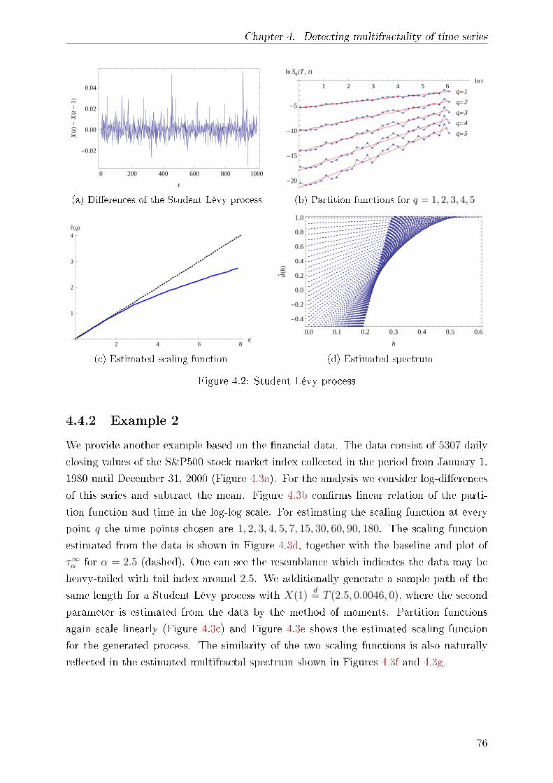
Chapter 4. Detecting multifractality of time series
0 200 400 600 800 1000
-0.02
0.00
0.02
0.04
t
XHtL-
XHt-
1L
(a) Dierences of the Student Lévy process
q=1
q=2
q=3
q=4
q=5
1 2 3 4 5 6ln t
-20
-15
-10
-5
ln SqHT , tL
(b) Partition functions for q = 1, 2, 3, 4, 5
2 4 6 8q
1
2
3
4Τ`HqL
(c) Estimated scaling function
0.0 0.1 0.2 0.3 0.4 0.5 0.6
-0.4
-0.2
0.0
0.2
0.4
0.6
0.8
1.0
h
d`HhL
(d) Estimated spectrum
Figure 4.2: Student Lévy process
4.4.2 Example 2
We provide another example based on the nancial data. The data consist of 5307 daily
closing values of the S&P500 stock market index collected in the period from January 1,
1980 until December 31, 2000 (Figure 4.3a). For the analysis we consider log-dierences
of this series and subtract the mean. Figure 4.3b conrms linear relation of the parti-
tion function and time in the log-log scale. For estimating the scaling function at every
point q the time points chosen are 1, 2, 3, 4, 5, 7, 15, 30, 60, 90, 180. The scaling function
estimated from the data is shown in Figure 4.3d, together with the baseline and plot of
τ∞α for α = 2.5 (dashed). One can see the resemblance which indicates the data may be
heavy-tailed with tail index around 2.5. We additionally generate a sample path of the
same length for a Student Lévy process with X(1)d= T (2.5, 0.0046, 0), where the second
parameter is estimated from the data by the method of moments. Partition functions
again scale linearly (Figure 4.3c) and Figure 4.3e shows the estimated scaling function
for the generated process. The similarity of the two scaling functions is also naturally
reected in the estimated multifractal spectrum shown in Figures 4.3f and 4.3g.
76
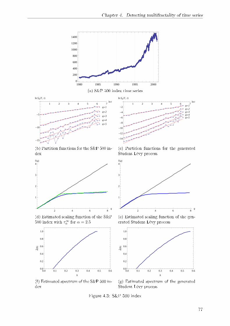
Chapter 4. Detecting multifractality of time series
1980 1985 1990 1995 20000
200
400
600
800
1000
1200
1400
(a) S&P 500 index time series
q=1
q=2
q=3
q=4
q=5
1 2 3 4 5 6 7ln t
-15
-10
-5
ln SqHT , tL
(b) Partition functions for the S&P 500 in-
dex
q=1q=2q=3q=4q=5
1 2 3 4 5 6 7ln t
-14
-12
-10
-8
-6
-4
-2
ln SqHT , tL
(c) Partition functions for the generated
Student Lévy process
2 4 6 8q
1
2
3
4Τ`HqL
(d) Estimated scaling function of the S&P
500 index with τ∞α for α = 2.5
2 4 6 8q
1
2
3
4Τ`HqL
(e) Estimated scaling function of the gen-
erated Student Lévy process
0.0 0.1 0.2 0.3 0.4 0.5 0.60.0
0.2
0.4
0.6
0.8
1.0
h
d`HhL
(f) Estimated spectrum of the S&P 500 in-
dex
0.0 0.1 0.2 0.3 0.4 0.5 0.60.0
0.2
0.4
0.6
0.8
1.0
h
d`HhL
(g) Estimated spectrum of the generated
Student Lévy process
Figure 4.3: S&P 500 index
77

Chapter 4. Detecting multifractality of time series
4.4.3 Conclusion
To briey summarize the main ndings of this section, we showed that the data coming
from heavy-tailed processes exhibit multifractal features. The rst conclusion from this
analysis is that one must be very careful when advocating multifractal model (like cascade
process or MRW) based on the shape of the estimated scaling function. A large class of
processes will behave as the moment scaling holds and this is hardly veriable in practice.
Even if the moment scaling does hold, heavy tails will produce concavity of the empirical
scaling function.
The nonlinearity of the estimated scaling function comes from estimating moments
that are actually innite. So it is obvious what we are doing wrong. The reasonable
solution one may suggest is to rst estimate the range of nite moments and then estimate
the scaling function only for this range, as otherwise moment scaling (4.5) does not make
sense. Therefore the rst step should be to estimate the tail index and suppose we
want to do this with the empirical scaling function as proposed in Chapter 2. For truly
multifractal processes, e.g. cascades, the estimated scaling function would be nonlinear
as there is nonlinear scaling and from the point of view of Chapter 2 this would lead us to
classify the data as heavy-tailed. Thus, we arrive at the converse problem: multifractal
processes with nonlinear scaling function may exhibit heavy tails. To illustrate this point
and to show that this problem is not restricted only to methods of Chapter 2, but appears
for other tail index estimators too, we present a simulation based example.
Example
Suppose X(t) is LNMRW with intermittency parameter λ2. We will analyze the distri-
bution tail of the increments of one sample path of such process. In nancial applications,
based on tting the estimated scaling function, parameter λ2 is usually taken around 0.05.
LNMRW is itself heavy-tailed (see Subsection 4.1.1) with the tail index equal to 1/λ2 and
for λ2 = 0.05 this gives the tail index value 20. Such large value is hardly observable
in practice and this has been a major critique of multifractal models in modeling asset
returns, as it is widely accepted that this data is heavy-tailed with the tail index between
3 and 5.
It has been observed rst in Calvet & Fisher (2004) that the data from multifractal
process may exhibit heavy-tailed properties with tail index much lower than its true value.
In Muzy et al. (2006), the authors provide a discussion based on the analogy with a certain
kind of physical system. They conclude, among other things, that estimating tail index
of the log-normal cascade (which is 1/(2λ2)) with the classical estimators such as Hill
and Pickands, will yield values around√(1− ν)/(2λ2). Here ν represents the log-ratio
of upper order statistics used in computing the estimator, i.e. ln k/ lnn for the sample
of size n. This means, for example, that if for the sample of size 10000 of the LNC with
78

Chapter 4. Detecting multifractality of time series
λ2 = 0.05 we compute the Hill estimator using k = 1000, instead of the true value 10, we
will get a value around 1.58.
2 4 6 8 10q
1
2
3
4
5ΤHqL
ΤLNMRWHqL
Τ`HqL
(a) Scaling functions
1 2 3 4-log
i
k + 1
1
2
3
4
5
logHXiL
(b) QQ plot with linear t
500 1000 1500 2000 2500k
1
2
3
4
5
6Α`
kHill
(c) Hill plot
500 1000 1500 2000 2500k
5
10
15
20Α`
kM
(d) Moment estimator plot
Figure 4.4: LNMRW generated with λ2 = 0.05
Let us illustrate this phenomenon with the sample path of LNMRW of length 10000
generated with λ2 = 0.05. Such process has nite moments up to order 20. Figure 4.4a
shows the estimated scaling function with the corresponding τLNMRW . From the point of
view of the results of Chapter 2, one may say that the scaling function exhibits nonlinearity
due to heavy-tails. However, the moments considered are nite and it is completely
legitimate to estimate them. One can observe the linearization eect as the discrepancy
between the two plots starting at around q = 6. Other methods also indicate heavy-tails.
QQ plot with k = 2000 (Figure 4.4b) shows approximate linearity and the estimated slope
is 1/2.31. The Hill plot shows very low values, although it is not very informative (Figure
4.4c). The moment estimator plot stabilizes around 5− 6 (Figure 4.4d). Following Muzy
et al. (2006), tail index estimators should correspond to√
2/λ2 ≈ 6.3 or lower, which is
conrmed in this case.
If we would adopt an estimate 3 or 4, the scaling function is almost linear for this
range and there would be no reason to consider multifractal models. To conclude, by
using empirical scaling functions it is impossible to distinguish whether the data are
heavy-tailed or multifractal.
79
Chapter 4. Detecting multifractality of time series
One of the goals of the statistical analysis of scaling properties is to distinguish whether
the data come from a process that is self-similar (4.2) or there is a more general multifractal
scaling (4.3). Both properties can be reduced to moment scaling (4.5) and described by the
scaling function, which is linear for self-similar processes and nonlinear for multifractals
dened by (4.3). This holds for a range of nite moments, otherwise, the denition of the
scaling function does not make sense. In theory, this is a completely clear distinction. In
practice, one estimates the scaling function using estimated moments. For this to work,
one must rst examine if the moments under consideration are nite. This is a serious
practical issue. First of all, this is a very challenging problem from the statistical point of
view. Secondly, the previous example shows that for the main examples of multifractals
the tail index is seriously underestimated. In the example considered, it is completely
legitimate to estimate the scaling function as the moments are nite, but the data itself
will behave dierently. So, determining a range of nite moments before estimation would
not be a good approach.
One may wonder if some other method may give better results. Wavelets are surely
the most widely used tool for the multifractal analysis. However, the same problem seems
to aect wavelets, as it is reported in Gonçalves & Riedi (2005). In this paper, the authors
propose a tail index estimator to determine the range of nite moments.
Before jumping to conclusion that the estimated scaling functions are not very useful,
one should remember that if the multifractal formalism holds, they can be used to estimate
the spectrum of singularities. It is to expect that the nonlinearities that are artefact of
the estimation method have nothing to do with the path properties. Although this is
generally true, some examples may suggest dierently. We leave this discussion for the
next chapter where we investigate the relation between moments and small scale path
properties.
80

Chapter 5
Moments and the spectrum of
singularities
As we have seen in the previous chapter, empirical scaling functions are not capable to de-
tect multifractal data as innite positive order moments are empirically indistinguishable
from multifractality. In this chapter we investigate the role of the scaling functions in the
multifractal formalism. For stochastic processes, multifractal formalism would mean that
it is possible to determine ne path properties using an object (scaling function) derived
from the process distribution. Moreover, this object, like moments, should be equally
dened for many, if not all processes. It is hard to believe that such general property may
hold. In this chapter, we make contribution to the problem by identifying properties that
make the spectrum nontrivial. We start with some motivating examples.
5.1 Motivation
Estimating innite positive order moments is what makes the empirical scaling function
to look misleading. However, the following examples suggest that if we are interested in
the spectrum of singularities, empirical scaling functions can be the right approach.
Suppose X(t) is a strictly α-stable Lévy process, 0 < α < 2. This process is 1/α-sssi
and has multifractal paths with spectrum given by (4.13). Scaling function τSLP is dened
on (−1, α) and τSLP (q) = q/α. The empirical scaling function asymptotically behaves as
τ∞α dened in Theorem 2, i.e.
τ∞α (q) =
qα, if 0 < q ≤ α,
1, if q > α.
If we consider Legendre transforms of these two functions and take inmum over all
81

Chapter 5. Moments and the spectrum of singularities
positive q where they are dened, then one can easily check that
inf0<q<α
(hq − τSLP (q) + 1) = inf0<q<∞
(hq − τ∞α (q) + 1) =
αh, if h ∈ [0, 1/α],
1, if h > 1/α.
This actually coincides with the true spectrum (4.13), except for the part h > 1/α, which
is the inmum obtained when q → 0. To correctly estimate this part one needs negative
order moments, which will be discussed later. Thus, although we are estimating innite
moments we arrive at the correct spectrum.
The second example is more compelling. Suppose X(t) is a LFSM with α ∈ [1, 2),
0 < H < 1 and H > 1/α. Since X(t) is H-sssi, the scaling function is τLFSM(q) = Hq
for q ∈ (−1, α). Theorem 3 justies estimating the scaling function in the same manner
as in Section 4.2 and Theorem 4 gives the asymptotic behavior:
τ∞H,α(q) =
Hq, if 0 < q ≤ α,(H − 1
α
)q + 1, if q > α.
Considering Legendre transform of τLFSM over (0, α) gives
inf0<q<α
(hq − τLFSM(q) + 1) =
α(h−H) + 1, if h ∈ [0, H],
1, if h > H.
Although the expression is similar to the true spectrum dLFSM dened in (4.15), the
support is dierent. On the other hand, it is easy to check that
inf0<q<∞
(hq − τ∞H,α(q) + 1
)=
−∞, if h < H − 1/α,
α(h−H) + 1, if h ∈ [H − 1/α,H],
1, if h > H.
Thus, the empirical scaling function will lead to a correct left part of the spectrum using
formalism. This reveals that the validity of the formalism may be narrow if τ is specied
as in (4.5). Secondly, it shows the potential of the empirical scaling function and indicates
that innite positive order moments may be related with path properties. To further sup-
port this conjecture, consider FBM. FBM is H-sssi with all positive order moments nite
and has a trivial spectrum consisting of only one point (4.12). This raises the question if
innite moments are what makes the spectrum of stable Lévy process and LFSM nontriv-
ial. We deal with this in the next section. The following example illustrates that generally
two properties are not related, however, the dierence with the previous examples is that
there is no exact scaling of nite dimensional distributions, like (4.1) or (4.3).
Suppose X(t), t ≥ 0 is a Lévy process. The Lévy processes in general do not satisfy
82
Chapter 5. Moments and the spectrum of singularities
moment scaling of the form (4.5). The only such examples are the BM and strictly α-
stable Lévy process. If X(1) is heavy-tailed and with zero mean, the empirical scaling
function will asymptotically behave as τ∞α dened in (2.4). On the other hand, spectrum
(4.14) depends on the BG index β. The estimated scaling function and the spectrum
are not related as they depend on the dierent parts of the Lévy measure. The shape
of the estimated scaling function is governed by the tail index, which depends on the
behavior of the Lévy measure π at innity since for q > 0, E|X(1)|q < ∞ is equivalent to∫|x|>1
|x|qπ(dx) < ∞. On the other hand, the spectrum is determined by the behavior of
π around origin, i.e. by the BG index. Stable Lévy processes are the special case since
then α = β.
5.1.1 Negative order moments
An example of the LNC suggests that to get the spectrum from the multifractal formalism,
negative order moments must also be included. Negative order moments depend on the
behavior of the distribution around 0. If taken for the increments of stochastic process,
they may describe small variations of paths. The problem with negative order moments is
that they are usually innite. For example, if random variable X has continuous density
f such that f(0) > 0, then E|X|−1 = ∞ and consequently, E|X|q = ∞ for every q ≤ −1.
However, if f is continuous and bounded near zero, then E|X|q < ∞ for every −1 < q < 0.
One can guess that innite negative order moments may also produce nonlinear be-
havior of the estimated scaling function. In the spirit of the previous discussion, one may
ask if these nonlinearities are related to the spectrum. We will show that this is not so in
the next section.
One of the rst references reporting this problem is Muzy et al. (1993), where the
authors introduced wavelet methods in the multifractal analysis. They proposed the
method called wavelet transform modulus maxima, which is based on a continuous wavelet
transform of a process where the partition function is dened by taking maxima over the
same scale wavelet transforms. Later the method based on wavelet leaders was introduced,
where the partition function is based on the local suprema of wavelet coecients (see e.g.
Jaard et al. (2007) and references therein). This resembles the method we propose in
Section 5.5, although our motivation comes entirely from the results of Section 5.2. Two
main advantages of the wavelet methods over the increments based partition function are
emphasized in the literature. First, wavelet leaders are more stable for divergent negative
order moments. In Section 5.5 we modify the partition function to have the same property
and this idea relies on the precise results about the spectrum. The second advantage is
the insensitivity of wavelets to polynomial trends, which makes it possible to study more
generally dened Hölder exponents (see Subsection 4.1.2). We conform to the denition
(4.10) in order to simplify the analysis and relate innite moments with path properties.
83

Chapter 5. Moments and the spectrum of singularities
5.2 Bounds on the support of the spectrum
Our goal in this section is to identify the property of the process that makes the spectrum
nontrivial. We do this by deriving the bounds on the support of the spectrum. The
lower bound is a consequence of the well-known Kolmogorov's continuity theorem. For
the upper bound we prove a sort of complement of this theorem.
Before we proceed, we x the following notation for a process X(t), t ∈ T where
T = [0, T ] or T = [0,+∞). We denote the range of nite moments as Q = (q, q), i.e.
q = supq > 0 : E|X(t)|q < ∞, ∀t,
q = infq < 0 : E|X(t)|q < ∞, ∀t.(5.1)
If X(t) is multifractal in the sense of Denition 2 with the scaling function τ dene
H− = sup
τ(q)
q− 1
q: q ∈ (0, q) & τ(q) > 1
,
H+ = inf
τ(q)
q− 1
q: q ∈ (q, 0) & τ(q) < 1
,
(5.2)
with the convention that sup ∅ = 0 and inf ∅ = +∞. In this context, we always assume
that (4.5) holds on the whole T and Q. All the processes X(t), t ∈ T considered here
are dened on some probability space (Ω,F , P ) and measurable, meaning that (t, ω) 7→X(t, ω) is B(T )×F -measurable. Furthermore, we assume that X(t), t ∈ T is separablewith respect to any dense countable set T ⊂ T , in the sense that for all t ∈ T there exists
a sequence (tn) in T, tn → t such that a.s. X(tn) → X(t). We say that the two processes
X(t), t ∈ T and X(t), t ∈ T dened on the same probability space are modications
of each other if for every t ∈ T , P (X(t) = X(t)) = 1. If P (X(t) = X(t), ∀t ∈ T ) = 1, we
say that the two processes are indistinguishable. Every stochastic process X(t), t ∈ T has a separable modication (see e.g. Doob (1953)).
5.2.1 The lower bound
Using the well-known Kolmogorov's criterion it is easy to derive the lower bound on the
support of the spectrum. Before stating the theorem, we dene f : T → R to be locally
Hölder continuous of order γ if for every compact K ⊂ T there exists a constant C(K)
such that
|f(t)− f(s)| ≤ C(K)|t− s|γ, ∀t, s ∈ K.
It is clear that the local Hölder continuity at some domain implies pointwise Hölder
continuity of the same order at any point. The proof of the following theorem can be
found in (Karatzas & Shreve 1991, Theorem 2.8) or (Kallenberg 2002, Theorem 3.23).
84
Chapter 5. Moments and the spectrum of singularities
Theorem 5 (Kolmogorov-Chentsov). Suppose that a process X(t), t ∈ T satises
E|X(t)−X(s)|α ≤ C|t− s|1+β, ∀t, s ∈ T , (5.3)
for some constants α > 0, β > 0 and C > 0. Then there exists a modication X(t), t ∈T of X(t), t ∈ T having continuous sample paths. Furthermore, a.s. X(t) is locally
Hölder continuous of order γ for every γ ∈ (0, β/α).
Proposition 1. Suppose X(t), t ∈ T is multifractal in the sense of Denition 2. If
τ(q) > 1 for some q ∈ (0, q), then there exists a modication of X(t) which is a.s.
locally Hölder continuous of order γ for every
γ ∈(0,
τ(q)
q− 1
q
).
In particular, there exists a modication such that a.s.
H− ≤ H(t), ∀t ∈ T ,
where H(t) is dened by (4.11) and H− by (5.2).
Proof. This is a simple consequence of Theorem 5 since Denition 2 implies
E|X(t)−X(s)|q = c(q)|t− s|1+(τ(q)−1).
For the second part, if H− = 0 there is nothing to prove. Otherwise, by (5.2), for each
γ < H− there is q ∈ (0, q) such that τ(q) > 1 and γ < (τ(q) − 1)/q, and thus, by the
rst part there is modication which is a.s. locally Hölder continuous of order γ. Since
all continuous modications are indistinguishable (see e.g. (Karatzas & Shreve 1991,
Problem 1.5), we have the desired modication. This implies that a.s. the pointwise
Hölder exponent is everywhere greater than H−.
In the sequel we always suppose to work with the modication from Proposition 1.
If H− > 0, we conclude that the spectrum d(h) = −∞ for h ∈ (0, H−). This way we
can establish an estimate for the left endpoint of the support of the spectrum. It also
follows that if the process is H-sssi and has nite moments of every positive order, then
H− = H ≤ H(t). Thus, when the moment scaling holds, path irregularities are closely
related with innite moments of positive order. We make this point stronger later.
Theorem 5 is valid for general stochastic processes. Although moment condition (5.3)
is appealing, the condition needed for the proof of Theorem 5 can be stated in a dierent
form.
Corollary 1. For a process X(t), t ∈ T there exists a modication which is a.s. locally
Hölder continuous of order γ > 0 if for some η > 1 it holds that for every K > 0 there
85

Chapter 5. Moments and the spectrum of singularities
exists C > 0 such that
lim supt→0
P (|X(s+ t)−X(s)| ≥ Ktγ)
tη≤ C, ∀s ∈ T .
Proof. This is obvious from the proof of Theorem 5; see (Karatzas & Shreve 1991, Theo-
rem 2.8).
5.2.2 The upper bound
To establish the bound on the right endpoint of the support of the spectrum, one needs to
show that a.s. the sample paths are nowhere Hölder continuous of some order γ, i.e. that
a.s. t 7→ X(t) /∈ Cγ(t0) for each t0 ∈ T . To show this we rst use a criterion based on
the negative order moments, similar to (5.3). The resulting theorem can be seen as a sort
of a complement of the Kolmogorov-Chentsov theorem. We then apply this to moment
scaling multifractals to get an estimate for the support of the spectrum.
In proving the statements involving negative order moments we use the following
two simple facts at several places. The rst is a Markov's inequality for negative order
moments. If X is a random variable, ε > 0 and q < 0, then
P (|X| ≤ ε) = P (|X|q ≥ εq) ≤ E|X|q
εq.
The second fact is the expression for the q-th order moment, q < 0,
E|X|q = −∫ ∞
0
qy−q−1P (1/|X| ≥ y)dy = −∫ ∞
0
qyq−1P (|X| ≤ y)dy.
Theorem 6. Suppose that a process X(t), t ∈ T satises
E|X(t)−X(s)|α ≤ C|t− s|1+β, ∀t, s ∈ T , (5.4)
for some constants α < 0, β < 0 and C > 0. Then a.s. X(t) is nowhere Hölder
continuous of order γ for every γ > β/α.
Proof. For typographical convenience we sometimes write Xt for X(t). First, it suces
to prove the statement by xing arbitrary γ > β/α. Indeed, this would give events Ωγ,
P (Ωγ) = 0 such that for ω ∈ Ω\Ωγ, t 7→ Xt(ω) is nowhere Hölder continuous of order γ.
If Ω0 is the union of Ωγ over all γ ∈ (β/α,∞) ∩ Q, then Ω0 ∈ F , P (Ω0) = 0 and Ω\Ω0
would t the statement of the theorem.
Secondly, it is enough to consider only restrictions to the interval [0, 1), as, if needed,
for n ∈ N we get from this the proof for the interval [n, n + 1) by using the process
X ′(t) = X(n + t) − X(n), t ∈ [0, 1). Removing null sets for all n ∈ N would imply the
general statement.
86

Chapter 5. Moments and the spectrum of singularities
For j, k ∈ N dene the set
Mjk :=∪
t∈[0,1)
∩h∈[0,1/k]
ω ∈ Ω : |Xt+h(ω)−Xt(ω)| ≤ jhγ .
It is clear that if ω /∈ Mjk for every j, k ∈ N, then t 7→ Xt(ω) is nowhere Hölder continuous
of order γ. As there is countably many Mjk, it is enough to x arbitrary j, k ∈ N and
show that Mjk ⊂ A for some A ∈ F such that P (A) = 0.
Suppose n > 2k and ω ∈ Mjk. Then there is some t ∈ [0, 1) such that
|Xt+h(ω)−Xt(ω)| ≤ jhγ, ∀h ∈ [0, 1/k]. (5.5)
Take i ∈ 1, . . . , n such thati− 1
n≤ t <
i
n. (5.6)
Since n > 2k we have
0 ≤ i
n− t <
i+ 1
n− t ≤ i+ 1
n− i− 1
n=
2
n<
1
k,
and from (5.5) it follows that
|X i+1n(ω)−X i
n(ω)| ≤ |X i+1
n(ω)−Xt(ω)|+ |Xt(ω)−X i
n(ω)| ≤ 2γ+1jn−γ.
Put A(n)i =
|X( i+1
n)−X( i
n)| ≤ 2γ+1jn−γ
. Since ω was arbitrary it follows that
Mjk ⊂n∪
i=1
A(n)i .
Using Markov's inequality for α < 0 and the assumption of the theorem we get
P (A(n)i ) ≤
E|X( i+1n)−X( i
n)|α
(2γ+1j)αn−γα≤ C(2γ+1j)−αnγα−1−β,
P
(n∪
i=1
A(n)i
)≤
n∑i=1
P (A(n)i ) ≤ C(2γ+1j)−αn−(β−γα).
(5.7)
If we set
A =∩n>2k
n∪i=1
A(n)i ,
then A ∈ F and Mjk ⊂ A. Since γ > β/α, it follows that β−γα > 0 and hence P (A) = 0.
This proves the theorem.
Proposition 2. Suppose X(t), t ∈ T is multifractal in the sense of Denition 2. If
τ(q) < 1 for some q ∈ (q, 0), then a.s. X(t) is nowhere Hölder continuous of order γ
87

Chapter 5. Moments and the spectrum of singularities
for every
γ ∈(τ(q)
q− 1
q, +∞
).
In particular, a.s.
H(t) ≤ H+, ∀t ∈ T .
Proof. Denition 2 implies
E|X(t)−X(s)|q = c(q)|t− s|1+(τ(q)−1).
Since q < 0, τ(q) < 0 and the statement follows from Theorem 6.
This proposition shows that d(h) = −∞ for h ∈ (H+,∞). Recall that H+ is dened
in (5.2).
Remark 5. Statements like the ones in Proposition 1 and 2 are stronger than saying, for
example, that for every t ∈ T , H(t) ≤ U a.s. Indeed, an application of the Fubini's
theorem would yield that for almost every path, H(t) ≤ U for almost every t. If we put
h = U + δ, then the Lebesgue measure of the set Sh = t : H(t) = h is zero a.s. This,
however, does not imply that d(h) = −∞ and hence, it is impossible to say something
about the spectrum of almost every sample path. On the other hand, it is clear that this
type of statements are implied by Propositions 1 and 2.
For the example of this weaker type of the bound, consider X(t),∈ T multifractal
in the sense of Denition 2. If there is q ∈ (q, 0), then for every t ∈ T
H(t) ≤ τ(q)
qa.s.
Indeed, let δ > 0 and suppose C > 0. Since q < 0, by Markov's inequality
P(|X(t+ ε)−X(t)| ≤ C|ε|
τ(q)q
+δ)≤ E |X(t+ ε)−X(t)|q
Cq|ε|τ(q)+δq=
c(q)
Cq|ε|δq→ 0,
as ε → 0. We can choose a sequence (εn) that converges to zero such that
P(|X(t+ εn)−X(t)| ≤ C|εn|
τ(q)q
+δ)≤ 1
2n.
Now, by the Borel-Cantelli lemma
|X(t+ εn)−X(t)|
|εn|τ(q)q
+δ→ ∞ a.s., as n → ∞.
Thus, for arbitrary δ > 0 it holds that for every t, H(t) ≤ τ(q)q
+ δ a.s. However, this
result does not allow us to say anything about the spectrum.
88
Chapter 5. Moments and the spectrum of singularities
Consider for the moment the FBM. The range of nite moments is (−1,∞) and
τ(q) = Hq for q ∈ (−1,∞), so we have H+ = H + 1. Thus, the best we can say from
Proposition 2, is that d(h) = −∞ for h > H + 1. However, we know that d(h) = −∞ for
h > H. If the inmum in the denition of H+ could be considered over all negative q, we
would get exactly the right endpoint of the support of the spectrum.
The fact that the bound derived in Proposition 2 is not sharp enough for some ex-
amples points that negative order moments may not be the right paradigm to explain
the spectrum. We therefore provide more general conditions that do not depend on the
niteness of moments. First of them is obvious from the proof of Theorem 6, Equation
(5.7).
Corollary 2. A process X(t), t ∈ T is a.s. nowhere Hölder continuous of order γ > 0
if for some η > 1 it holds that for every K > 0 there exists C > 0 such that
lim supt→0
P (|X(s+ t)−X(s)| ≤ Ktγ)
tη≤ C, ∀s ∈ T .
Theorem 7. A process X(t), t ∈ T is a.s. nowhere Hölder continuous of order γ > 0
if for some η > 1 and m ∈ N it holds that for every K > 0 there exists C > 0 such that
lim supt→0
P
(max
l=1,...,m|X(s+ lt)−X(s+ (l − 1)t)| ≤ Ktγ
)tη
≤ C, ∀s ∈ T . (5.8)
Proof. The rst part of the proof goes exactly as in the proof of Theorem 6. Fix j, k ∈ Nand take n ∈ N such that
n > (m+ 1)k.
If ω ∈ Mjk, then there is some t ∈ [0, 1) and i ∈ 1, . . . , n such that (5.5) and (5.6) hold.
Choice of n ensures that for l ∈ 1, . . . ,m
0 <i+ l − 1
n− t <
i+ l
n− t <
i+ l
n− i− 1
n=
l + 1
n≤ 1
k.
It follows from (5.5) that for each l ∈ 1, . . . ,m
|X i+ln(ω)−X i+l−1
n(ω)| ≤ j
(l + 1
n
)γ
+ j
(l
n
)γ
≤ 2j
(m+ 1
n
)γ
.
Let
A(n)i,l =
|X( i+l
n)−X( i+l−1
n)| ≤ 2j
(m+1n
)γ,
A(n)i =
m∩l=1
A(n)i,l .
89

Chapter 5. Moments and the spectrum of singularities
It then follows that
Mjk ⊂n∪
i=1
A(n)i .
From the assumption, there exists C > 0 such that
P (A(n)i ) = P
(max
l=1,...,m|X( i+l
n)−X( i+l−1
n)| ≤ 2j(m+ 1)γ
(1n
)γ) ≤ Cn−η,
P
(n∪
i=1
A(n)i
)≤
n∑i=1
P (A(n)i ) ≤ Cn−(η−1).
Now setting
A =∩
n>(m+1)k
n∪i=1
A(n)i ∈ F ,
it follows that P (A) = 0, since η > 1.
Theorem 7 enables one to avoid using moments in deriving the bound. As an example,
we consider how Theorem 7 can be applied in the simple case when X(t) is BM. Since
X(t) is 1/2-sssi we have
P
(max
l=1,...,m|X(lt)−X((l − 1)t)| ≤ Ktγ
)= P
(max
l=1,...,m|X(l)−X(l − 1)| ≤ Ktγ−1/2
).
Due to independent increments:
P
(max
l=1,...,m|X(l)−X(l − 1)| ≤ Ktγ−1/2
)=(P(|X(1)| ≤ Ktγ−1/2
))m ≤ Ctm(γ−1/2).
This holds for every γ > 1/2 and m ∈ N and by taking m > 1/(γ−1/2) we conclude that
d(h) = −∞ for h > 1/2.
Before we proceed on applying these results, we state the following simple corollary
that expresses the criterion (5.8) in terms of the negative order moments, but now mo-
ments of the maximum of increments. This is a generalization of Theorem 6, which
enables bypassing innite negative order moments under very general conditions. From
this criterion, in the next section we derive strong statements about H-sssi processes.
Corollary 3. Suppose that a process X(t), t ∈ T satises
E
[max
l=1,...,m|X(s+ lt)−X(s+ (l − 1)t)|
]α≤ Ct1+β, ∀t, s ∈ T , (5.9)
for some α < 0, β < 0, m ∈ N and C > 0. Then a.s. X(t) is nowhere Hölder
continuous of order γ for every γ > β/α.
Proof. This follows directly from the Markov's inequality for negative order moments and
90

Chapter 5. Moments and the spectrum of singularities
Theorem 7 since
P
(max
l=1,...,m|X(s+ lt)−X(s+ (l − 1)t)| ≤ Ktγ
)≤ K−αt−γαE
[max
l=1,...,m|X(s+ lt)−X(s+ (l − 1)t)|
]α≤ K−αCt−αγ+1+β,
and 1 + β − αγ > 1.
5.3 Applications
In this section we consider in more details processes with scaling properties and apply
the results of the previous section to derive some very general statements about these
processes.
5.3.1 The case of self-similar stationary increments processes
In this subsection we rene our results for the case of H-sssi processes by using Corollary
3. These results can also be viewed in the light of the classical papers Vervaat (1985)
and Takashima (1989). To be able to apply Corollary 3, we need to make sure that the
moment in (5.9) can be made nite by choosing m large enough. We state this condition
explicitly for reference.
Condition 1. Suppose X(t), t ∈ T is a stationary increments process. For every α < 0
there is m0 ∈ N such that
E
[max
l=1,...,m0
|X(l)−X(l − 1)|]α
< ∞.
One way of assessing the Condition 1 is given in the following lemma, which is strong
enough to cover all the examples considered later. Recall the denition of the range of
nite moments q and q given in (5.1).
Lemma 3. Suppose X(t), t ≥ 0 is a stationary increments process which is ergodic in
the sense that if E|f(X1)| < ∞ for some measurable f , then∑ml=1 f(Xl −Xl−1)
m
a.s.→ Ef(X1), as m → ∞.
Suppose also that q < 0. Then Condition 1 holds.
91
Chapter 5. Moments and the spectrum of singularities
Proof. Let r < 0 be such that E|X(1)−X(0)|r < ∞. Then
infl∈N
|X(l)−X(l − 1)|r = limm→∞
minl=1,...,m
|X(l)−X(l − 1)|r
≤ limm→∞
∑ml=1 |X(l)−X(l − 1)|r
m= E|X(1)−X(0)|r =: M a.s.
For α < 0 it follows
infl∈N
|X(l)−X(l − 1)|α =
(infl∈N
|X(l)−X(l − 1)|r)α
r
≤ Mαr a.s.
and inf l∈N |X(l)−X(l− 1)|α is bounded and thus has nite expectation. Given α < 0 we
can choose m0 such that[max
l=1,...,m0
|X(l)−X(l − 1)|]α
=
[1
maxl=1,...,m0 |X(l)−X(l − 1)|
]−α
=
[min
l=1,...,m0
1
|X(l)−X(l − 1)|
]−α
= minl=1,...,m0
|X(l)−X(l − 1)|α ≤ Mαr a.s.,
which implies the statement.
Remark 6. Two examples may provide insight of how far the assumptions of Lemma 3
are from Condition 1. If X(t) = tX for some random variable X, then
maxl=1,...,m
|X(l)−X(l − 1)| = X
and thus, Condition 1 depends on the range of nite moments of X. For the second
example, suppose X(l)−X(l− 1) is an i.i.d. sequence such that P (|X(1)−X(0)| ≤ x) =
− ln 2/ lnx for x ∈ (0, 1/2). This implies, in particular, that E|X(1) − X(0)|r = ∞ for
any r < 0. Moreover,
E
[max
l=1,...,m|X(l)−X(l − 1)|
]α= −
∫ ∞
0
αyα−1P
(max
l=1,...,m|X(l)−X(l − 1)| ≤ y
)dy
= −∫ ∞
0
αyα−1 1
(ln y)mdy = ∞,
for every α < 0 and m ∈ N, thus Condition 1 does not hold.
We are now ready to prove a general theorem about H-sssi processes.
Theorem 8. Suppose X(t), t ≥ 0 is H-sssi stochastic process such that Condition 1
holds and H − 1/q ≥ 0. Then a.s.
H − 1
q≤ H(t) ≤ H, ∀t ≥ 0.
92

Chapter 5. Moments and the spectrum of singularities
Proof. By the same argument as in the beginning of the proof of Theorem 6 it is enough to
take arbitrary γ > H. Given γ we take α < 1/(H−γ) < 0 which implies γ > H−1/α. Due
to Condition 1, we can choose m0 ∈ N such that E [maxl=1,...,m0 |X(lt)−X((l − 1)t)|]α <
∞. Self-similarity then implies that
E
[max
l=1,...,m0
|X(lt)−X((l − 1)t)|]α
= tHαE
[max
l=1,...,m0
|X(l)−X(l − 1)|]α
= Ct1+(Hα−1).
The claim now follows immediately from Corollary 3 with β = Hα−1 since γ > β/α.
A simple consequence of the preceding is the following statement.
Corollary 4. Suppose that Condition 1 holds. A H-sssi process with all positive order
moments nite has a trivial spectrum, i.e. d(h) = −∞ for h = H.
This applies to FBM, but also to all Hermite processes, like e.g. Rosenblatt process
(see Section 5.4). Thus, under very general conditions a self-similar stationary increments
process with a nontrivial spectrum must be heavy-tailed. This shows clearly how innite
moments can aect path properties when the scaling holds. The following simple result
shows this more precisely.
Proposition 3. Suppose X(t), t ≥ 0 is H-sssi. If γ < H and d(γ) = −∞, then
E|X(1)|q = ∞ for q > 1/(H − γ).
Proof. Suppose E|X(t)|q < ∞ for q > 1/(H − γ). Then for ε > 0 we can apply Markov's
inequality to get
P (|X(t)| ≥ Ktγ) = P(|X(1)| ≥ Ktγ−H
)≤ E |X(1)|
1H−γ
+ε
K1
H−γ+εt−1−ε(H−γ)
≤ Ct1+ε(H−γ).
By Corollary 1 this implies d(γ) = −∞, which is a contradiction.
5.3.2 The case of multifractal processes
Our next goal is to show that in the denition of H+ one can essentially take the inmum
over all q < 0. At the moment this makes no sense as τ from Denition 2 may not be
dened in this range. It is therefore necessary to redene the meaning of the scaling
function and thus we work with the more general Denition 1.
In the next section we will see on the example of the LNC process that when the mul-
tifractal process has all negative order moments nite, the bound derived in Proposition 2
is sharp. In general, this would not be the case for any multifractal in the sense of Deni-
tion 1. Take for example a LNMRW, which is a compound process X(t) = B(θ(t)) where
B is BM and θ is an independent LNC. By the multifractality of the cascade for t < 1,
θ(t) =d M(t)θ(1) and multifractality of LNMRW implies X(t) =d (M(t)θ(1))1/2B(1).
93
Chapter 5. Moments and the spectrum of singularities
Now by the independence of B and θ, if E|B(1)|q = ∞, then E|X(t)|q = ∞. Since B(1)
is Gaussian, the moments will be innite for q ≤ −1.
We thus provide a more general bound which only has a restriction on the moments
of the random factor from Denition 1. Therefore, if the process satises Denition 1 and
if the random factor M is multifractal by Denition 2 with scaling function τ , we dene
H+ = inf
τ(q)
q− 1
q: q < 0 & E|M(t)|q < ∞
.
Corollary 5. Suppose X(t), t ∈ T has stationary increments and Condition 1 holds.
Suppose also it is multifractal by Denition 1 and the random factor M satises Denition
2 with scaling function τ . If E|M(t)|q < ∞, ∀t ∈ T for some q < 0, then a.s. X(t) is
nowhere Hölder continuous of order γ for every
γ ∈(τ(q)
q− 1
q, +∞
).
In particular, a.s.
H(t) ≤ H+, ∀t ∈ T .
Proof. By Condition 1 for m large enough it follows from the multifractal property (4.3)
that
E
[max
l=1,...,m|X(lt)−X((l − 1)t)|
]q= E|M(t)|qE
[max
l=1,...,m|X(l)−X(l − 1)|
]q= Ct1+τ(q)−1.
The claim now follows from Corollary 3 with α = q and β = τ(q)−1 and by the argument
at the beginning of the proof of Theorem 6.
In summary, we provide bounds on the support of the multifractal spectrum. We
show that the lower bound can be derived using positive order moments and link innite
moments with path properties for the case of H-sssi process. In general, negative order
moments are not appropriate for explaining the right part of the spectrum. To derive
an upper bound on the support of the spectrum, we use negative order moments of the
maximum of increments. This avoids the nonexistence of the negative order moments,
which is a property of the distribution itself.
5.4 Examples
In this section we list several examples of stochastic processes and investigate how the
results of Sections 5.2 and 5.3 apply in these cases. We also discuss how the multifractal
formalism could be achieved.
94

Chapter 5. Moments and the spectrum of singularities
5.4.1 Self-similar processes
It follows from Theorem 8 and Corollary 4 that if H-sssi process is ergodic with nite
positive order moments, then the spectrum is simply
d(h) =
1, if h = H
−∞, otherwise.
This applies to all Hermite processes, e.g. BM, FBM and Rosenblatt process. Hermite
process Z(k)H (t), t ≥ 0 with H ∈ (1/2, 1) and k ∈ N can be dened as
Z(k)H (t) = C(H, k)
∫ ′
Rk
∫ t
0
(k∏
j=1
(s− yj)−( 1
2+ 1−H
k)
+
)dsdB(y1) · · · dB(yk), t ≥ 0,
where B(t) is the standard BM and the integral is taken over Rk except the hyperplanes
yi = yj, i = j. The constant C(H, k) is chosen such that E[Z(k)H (1)]2 = 1 and (x)+ =
max(x, 0). Hermite processes are H-sssi. For k = 1 one gets the FBM and for k = 2 the
Rosenblatt process. See Embrechts & Maejima (2002) for more details.
Hermite processes have all positive order moments nite and the increments are ergodic
(see e.g. (Samorodnitsky 2007, Section 7)), so they have a trivial spectrum. The spectrum
of Hermite processes has been studied so far only numerically (Wendt et al. (2012)). We
now discuss heavy tailed examples of H-sssi processes.
Stable Lévy processes
As already discussed in Section 5.1, the spectrum of a strictly α-stable Lévy process is
nontrivial and supported on [0, 1/α]. These are exactly the bounds given in Theorem 8
as in this case H = 1/α and q = α.
Linear fractional stable motion
The spectrum of the LFSM for α ∈ [1, 2), H ∈ (0, 1) and in the long-range dependence
case H > 1/α is supported on [H − 1α, H]. Also, increments of the LFSM are ergodic (see
e.g. Cambanis et al. (1987)). Since q = α, sharp bounds on the support of the spectrum
follow from Theorem 8.
Inverse stable subordinator
Lévy process Y (t), t ≥ 0 such that Y (1) ∼ Sα(σ, 1, 0), 0 < α < 1 is called the stable
subordinator. It is nondecreasing and 1/α-sssi. The inverse stable subordinator X(t), t ≥0 is dened as
X(t) = inf s > 0 : Y (s) > t .
95

Chapter 5. Moments and the spectrum of singularities
It is α-ss with dependent, nonstationary increments, nondecreasing and corresponds to
the rst passage time of the stable subordinator strictly above level t. For more details
see Meerschaert & Straka (2013) and references therein.
The application of the results of the previous section for the inverse stable subordinator
is not straightforward as it has nonstationary increments, yet we can prove that it has a
trivial spectrum such that d(α) = 1.
To derive the lower bound we use Theorem 5. First recall that aα + bα ≤ (a+ b)α for
a, b ≥ 0 and α ∈ (0, 1). Taking a = t − s, b = s when t ≥ s and a = t, b = s − t when
t < s gives that |tα − sα| ≤ |t − s|α. Since X(t) has nite moments of every positive
order we have for arbitrary q > 0 and t, s > 0
E|X(t)−X(s)|q = |tα − sα|qE|X(1)|q ≤ E|X(1)|q|t− s|1+αq−1.
By Theorem 5 there exists modication which is a.s. locally Hölder continuous of order
γ < α−1/q. Since q can be taken arbitrarily large, we can get the modication such that
a.s. H(t) ≥ α for every t ≥ 0.
For the upper bound we use Theorem 7. Given γ > α we choose m ∈ N such that
m > 1/(γ − α). If Y (t) is the corresponding stable subordinator, from the property
X(t) ≤ a = Y (a) ≥ t we have for every t1 < t2 and a > 0
X(t2)−X(t1) ≤ a = YX(t1)+a ≥ t2 = YX(t1)+a − t1 ≥ t2 − t1.
By (Bertoin 1998, Theorem 4, p. 77), for every t1 > 0, P (YX(t1) > t1) = 1, thus, on this
event
YX(t1)+a − t1 ≥ t2 − t1 ⊂ YX(t1)+a − YX(t1) ≥ t2 − t1.
Now by the strong Markov property choosing t small enough and stationarity of increments
of Y (t) we have
P
(max
l=1,...,m|X(s+ lt)−X(s+ (l − 1)t)| ≤ Ktγ
)= P (X(s+ t)−X(s) ≤ Ktγ, . . . , X(s+mt)−X(s+ (m− 1)t) ≤ Ktγ)
≤ P(YX(s)+Ktγ − YX(s) ≥ t, . . . , YX(s+(m−1)t)+Ktγ − YX(s+(m−1)t) ≥ t
)≤ (P (Y (Ktγ) ≥ t))m =
(P(Y (1) ≥ K− 1
α t1−γα
))m≤(Ctγ−α
)m,
by the regular variation of the tail for t suciently small. Due to the choice of m,
m(γ−α) > 1. This property of the rst-passage process has been noted in (Bertoin 1998,
p. 96).
96

Chapter 5. Moments and the spectrum of singularities
5.4.2 Lévy processes
Suppose X(t), t ≥ 0 is a Lévy process. The Lévy processes in general do not satisfy
the moment scaling of the form (4.5). As there is no exact moment scaling, Propositions
1 and 2 cannot be applied. Thus, in order to establish bounds on the support of the
spectrum we use other criteria from Section 5.2. We present two analytically tractable
examples to illustrate the use of these criteria.
Inverse Gaussian Lévy process
The inverse Gaussian Lévy process is a subordinator such that X(1) has an inverse Gaus-
sian distribution IG(δ, λ), δ > 0, λ ≥ 0, given by the density
f(x) =δ√2π
eδλx−3/2 exp
−1
2
(δ2
x+ λ2x
), x > 0.
The expression for the cumulant reveals that for each t, X(t) has IG(tδ, λ) distribution.
Lévy measure is absolutely continuous with the density given by
g(x) =δ√2π
x−3/2 exp
−λ2x
2
, x > 0,
thus, the BG index is β = 1/2. See Eberlein & v. Hammerstein (2004) for more details.
Inverse Gaussian distribution has moments of every order nite and for every q ∈ R we
can express them as
E|X(1)|q =∫ ∞
0
xqf(x)dx =δ√2π
eδλ(
2
λ2
)q−1/2 ∫ ∞
0
xq−3/2 exp
−x− δ2λ2
4x
dx
=δ√2π
eδλ(
2
λ2
)q−1/2
K−q+ 12(δλ)2
(δλ
2
)q− 12
=
√2
πeδλδq+
12λ−q+ 1
2K−q+ 12(δλ),
where we have used (Olver et al. 2010, Equation 10.32.10) and Kν denotes the modied
Bessel function of the second kind. This implies that
E|X(t)|q =√
2
πetδλtq+
12 δq+
12λ−q+ 1
2K−q+ 12(tδλ) ∼ Ctq+
12 t−|−q+ 1
2|, as t → 0,
since Kν(z) ∼ 12Γ(ν)(1
2z)−ν for z > 0 and K−ν(z) = Kν(z). For any choice of γ > 0
condition of Corollary 1 cannot be fullled, so the best we can say is that the lower bound
is 0, in accordance with (4.14). Since negative order moments are nite, Corollary 2
yields the sharp upper bound on the spectrum. Indeed, given γ > 1/β = 2 we have for
q < 1/(2− γ) < 0
P (|X(t)| ≤ Ktγ) ≤ E|X(t)|q
Kqtγq≤ Ct−q(γ−2),
97

Chapter 5. Moments and the spectrum of singularities
for t suciently small. It follows that the upper bound is 2 which is exactly the reciprocal
of the BG index.
Tempered stable subordinator
The positive tempered stable distribution is obtained by exponentially tilting the Lévy
density of the α-stable distribution, 0 < α < 1. The tempered stable subordinator is a
Lévy process X(t) such that X(1) has a positive tempered stable distribution given by
the cumulant function
Φ(θ) = logE[e−θX(1)
]= δλ− δ
(λ1/α + 2θ
)α, θ ≥ 0,
where δ is the scale parameter of the stable distribution and λ is the tilt parameter. In
this case BG index is equal to α (see Schoutens (2003) for more details). We use Corollary
2 for γ > α to get
P (|X(t)| ≤ Ktγ) ≤ eE[e−
X(t)Ktγ
]= e1+tΦ(K−1t−γ) = O(e−t1−γ/α
), as t → 0.
As this decays faster than any power of t as t → 0, the upper bound follows.
5.4.3 Multifractal processes
In this subsection, results are applied to examples of processes that are multifractal by
Denition 1 and 2.
Log-normal cascade
We rst analyze the log-normal cascade process. The spectrum of the LNC is supported
on the interval[1 + 2λ2 − 2
√2λ2, 1 + 2λ2 + 2
√2λ2], as follows from (4.16).
The condition τ(q) > 1 of Proposition 1 yields q ∈ (1, 1/(2λ2)). We then get that
H− = 1 + 2λ2 − 2√2λ2.
This is exactly the left endpoint of the interval where the spectrum of the cascade is nite,
in accordance with Proposition 1. This maximal lower bound is achieved for q = 1/√2λ2,
which by (4.24) is exactly the point q+0 at which the linearization eect occurs. If q− is
the point at which the maximal lower bound H− is achieved, then(τ(q)
q− 1
q
)′
=1
q2(qτ ′(q)− τ(q) + 1)
must be equal to 0 at q−. This is exactly dened in (4.23). Although the range of nite
moments is not relevant for computing H− in this case, in general it can depend on q.
98

Chapter 5. Moments and the spectrum of singularities
For the upper bound, since all negative order moments are nite we get that
H+ = H+ = 1 + 2λ2 + 2√2λ2
achieved for q = −1/√2λ2, which is equal to q−0 from (4.25). Thus, again, the bound
from Proposition 2 is sharp, giving the right endpoint of the interval where the spectrum
is supported.
Log-normal multifractal random walk
The example of LNMRW illustrates that we may have H+ = H+ and that the denition
of the scaling function needs to be adjusted to avoid innite moments of negative order.
The scaling function is dened for the range of nite moments, which is (−1, 1/λ2) as
explained earlier. However, if we consider τ as the scaling function of the random factor
M(c) = c1/2eΓc dened in (4.8), then the denition of τ makes sense for all q ∈ (−∞, 1/λ2).
The spectrum is supported on the interval[1/2 + λ2 −
√2λ2, 1/2 + λ2 +
√2λ2]and given
by (4.17).
The random factor M(c) is the source of multifractality, has the same scaling function
(4.9), but all negative order moments are nite. Thus we get
H− = 1/2 + λ2 −√2λ2,
H+ =3
2+
3λ2
2,
H+ = 1/2 + λ2 +√2λ2.
H− and H+ give the sharp bounds, while H+ is aected by the divergence of negative
order moments. This shows that when the multifractal process has innite negative order
moments, one should specify scaling in terms of the random factor. The optimal bounds
H− and H+ are attained for q− =√2/λ2 and q+ = −
√2/λ2, respectively.
5.5 Robust version of the partition function
In Section 5.2 using Corollary 3 we managed to avoid the problematic innite moments
of negative order and prove results like Theorem 8 and Corollary 5. When the scaling
function (1.4) is estimated from the data, spurious concavity may appear for negative
values of q, due to the eect of diverging negative order moments. We use the idea of
Corollary 3 to develop a more robust version of the partition function.
Instead of using increments in the partition function (1.2), we can use the maximum
of some xed number m of the same length increments. This will make the negative order
moments nite for some reasonable range and prevent divergencies. The underlying idea
99

Chapter 5. Moments and the spectrum of singularities
resembles the wavelet leaders method, where leaders are formed as the maxima of the
wavelet coecients over some time scale (see Jaard et al. (2007)). Since m is xed, this
does not aect the true scaling. The same idea can be used for q > 0 by an argument
following from Corollary 1. It is important to stress that the estimation of the scaling
function makes sense only if the underlying process is known to possess scaling property
of the type (4.3).
Suppose X(t) has stationary increments and X(0) = 0. Divide the interval [0, T ]
into ⌊T/(mt)⌋ blocks each consisting of m increments of length t and dene the modied
partition function:
Sq(T, t) =1
⌊T/(mt)⌋
⌊T/(mt)⌋∑i=1
maxl=1,...,m
|X(imt+ lt)−X(imt+ (l − 1)t)|q . (5.10)
One can see Sq(T, t) as a natural estimator of the moment in (5.9). Analogously we dene
the modied scaling function as in (1.4) by using Sq(n, ti):
τN,T (q) =
∑Ni=1 ln ti ln Sq(n, ti)− 1
N
∑Ni=1 ln ti
∑Nj=1 ln Sq(n, ti)∑N
i=1 (ln ti)2 − 1
N
(∑Ni=1 ln ti
)2 . (5.11)
The denition can be altered only for q < 0 although there is no much dierence between
two forms when q > 0.
To illustrate how this modication makes the scaling function more robust we present
several examples comparing (1.4) and (5.11). We generate sample paths of several pro-
cesses and estimate the scaling function by both methods. We also estimate the spectrum
numerically using (4.18). The results are shown in Figures 5.1-5.4. Each gure shows the
estimated scaling functions and the estimated spectrum by using standard denition (1.4)
and by using (5.11). We also added the plots of the scaling function that would yield the
correct spectrum via multifractal formalism and the true spectrum of the process.
For the BM (Figure 5.1) and the α-stable Lévy process (Figure 5.2) we generated
sample paths of length 10000 and used α = 1 for the latter. LFSM (Figure 5.3) was
generated using H = 0.9 and α = 1.2 with path length 15784. Finally, the sample path of
the LNMRW of length 10000 was generated with λ2 = 0.025 (Figure 5.4). For each case
we take m = 20 in dening the modied partition function (5.10).
In all the examples considered, the modied scaling function is capable of yielding
the correct spectrum of the process with the multifractal formalism. As opposed to the
standard denition, it is unaected by diverging negative order moments. Moreover, it
captures the divergence of positive order moments which determines the shape of the
spectrum.
100

Chapter 5. Moments and the spectrum of singularities
-4 -2 2 4
-6
-4
-2
2
ΤHqL
ΤHqL
Τ`HqL
(a) Scaling functions
0.0 0.2 0.4 0.6 0.8 1.00.0
0.2
0.4
0.6
0.8
1.0
dHqL
d
HqL
d`
HqL
(b) Spectrum
Figure 5.1: Brownian motion
-3 -2 -1 1 2 3
-4
-3
-2
-1
1
ΤHqL
ΤHqL
Τ`HqL
(a) Scaling functions
0.0 0.5 1.0 1.5 2.00.0
0.2
0.4
0.6
0.8
1.0
dHqL
d
HqL
d`
HqL
(b) Spectrum
Figure 5.2: Stable Lévy process α = 1
-3 -2 -1 1 2 3
-4
-3
-2
-1
1
ΤHqL
ΤHqL
Τ`HqL
(a) Scaling functions
0.0 0.5 1.0 1.5 2.00.0
0.2
0.4
0.6
0.8
1.0
dHqL
d
HqL
d`
HqL
(b) Spectrum
Figure 5.3: LFSM H = 0.9, α = 1.2
101

Chapter 5. Moments and the spectrum of singularities
-10 -5 5 10
-15
-10
-5
ΤHqL
ΤHqL
Τ`HqL
(a) Scaling functions
0.0 0.5 1.0 1.50.0
0.2
0.4
0.6
0.8
1.0
dHqL
d
HqL
d`
HqL
(b) Spectrum
Figure 5.4: LNMRW λ2 = 0.025
102

Bibliography
Abry, P., Chainais, P., Coutin, L. & Pipiras, V. (2009), `Multifractal random walks as
fractional Wiener integrals', Information Theory, IEEE Transactions on 55(8), 3825
3846.
Alsmeyer, G., Biggins, J. & Meiners, M. (2012), `The functional equation of the smoothing
transform', The Annals of Probability 40(5), 20692105.
Anh, V. V., Leonenko, N. N. & Shieh, N.-R. (2008), `Multifractality of products of geomet-
ric Ornstein-Uhlenbeck-type processes', Advances in Applied Probability 40(4), 1129
1156.
Anh, V. V., Leonenko, N. N. & Shieh, N.-R. (2009a), `Multifractal products of stationary
diusion processes', Stochastic Analysis and Applications 27(3), 475499.
Anh, V. V., Leonenko, N. N. & Shieh, N.-R. (2009b), `Multifractal scaling of products of
birth-death processes', Bernoulli 15(2), 508531.
Anh, V. V., Leonenko, N. N., Shieh, N.-R. & Taufer, E. (2010), `Simulation of multifractal
products of Ornstein-Uhlenbeck type processes', Nonlinearity 23(4), 823843.
Avram, F., Leonenko, N. & uvak, N. (2013), `On spectral analysis of heavy-tailed
Kolmogorov-Pearson diusions', Markov Processes and Related Fields 19(2), 249298.
Ayache, A. & Hamonier, J. (2012), `Linear fractional stable motion: A wavelet estimator
of the α parameter', Statistics & Probability Letters 82(8), 15691575.
Ayache, A. & Hamonier, J. (2013), `Linear multifractional stable motion: wavelet estima-
tion of H(·) and α parameters', arXiv preprint arXiv:1304.2995 .
Bacry, E., Delour, J. & Muzy, J.-F. (2001), `Multifractal random walk', Physical Review
E 64(2), 026103.
Bacry, E., Gloter, A., Homann, M. & Muzy, J. F. (2010), `Multifractal analysis in a
mixed asymptotic framework', The Annals of Applied Probability 20(5), 17291760.
103

Bibliography
Bacry, E., Kozhemyak, A. & Muzy, J. (2013), `Log-normal continuous cascade model of
asset returns: aggregation properties and estimation', Quantitative Finance 13(5), 795
818.
Bacry, E., Kozhemyak, A. & Muzy, J.-F. (2008), `Continuous cascade models for asset
returns', Journal of Economic Dynamics and Control 32(1), 156199.
Bacry, E. & Muzy, J. F. (2003), `Log-innitely divisible multifractal processes', Commu-
nications in Mathematical Physics 236(3), 449475.
Balança, P. (2014), `Fine regularity of Lévy processes and linear (multi)fractional stable
motion', Electronic Journal of Probability 19(101), 137.
Barral, J., Fournier, N., Jaard, S. & Seuret, S. (2010), `A pure jump Markov process
with a random singularity spectrum', The Annals of Probability 38(5), 19241946.
Barral, J. & Jin, X. (2014), `On exact scaling log-innitely divisible cascades', Probability
Theory and Related Fields 160(3-4), 521565.
Barral, J. & Mandelbrot, B. B. (2002), `Multifractal products of cylindrical pulses', Prob-
ability Theory and Related Fields 124(3), 409430.
Barral, J. & Seuret, S. (2007), `The singularity spectrum of Lévy processes in multifractal
time', Advances in Mathematics 214(1), 437468.
Barunik, J., Aste, T., Di Matteo, T. & Liu, R. (2012), `Understanding the source of mul-
tifractality in nancial markets', Physica A: Statistical Mechanics and its Applications
391(17), 42344251.
Beirlant, J., Goegebeur, Y., Segers, J. & Teugels, J. (2006), Statistics of extremes: theory
and applications, Wiley, New York.
Bertoin, J. (1998), Lévy processes, Cambridge University Press, Cambridge.
Bibby, B. M., Skovgaard, I. M. & Sørensen, M. (2005), `Diusion-type models with given
marginal distribution and autocorrelation function', Bernoulli 19(2), 191220.
Calvet, L. E. & Fisher, A. J. (2004), `How to forecast long-run volatility: Regime switch-
ing and the estimation of multifractal processes', Journal of Financial Econometrics
2(1), 4983.
Calvet, L. E. & Fisher, A. J. (2008), Multifractal volatility: theory, forecasting, and pric-
ing, Academic Press, New York.
Calvet, L. & Fisher, A. (2002), `Multifractality in asset returns: theory and evidence',
Review of Economics and Statistics 84(3), 381406.
104

Bibliography
Cambanis, S., Hardin Jr, C. D. & Weron, A. (1987), `Ergodic properties of stationary
stable processes', Stochastic Processes and their Applications 24(1), 118.
Chainais, P., Riedi, R. & Abry, P. (2005), `On non-scale-invariant innitely divisible
cascades', Information Theory, IEEE Transactions on 51(3), 10631083.
De Haan, L. & Ferreira, A. (2007), Extreme value theory: an introduction, Springer, New
York.
Dekkers, A., Einmahl, J. & De Haan, L. (1989), `A moment estimator for the index of an
extreme-value distribution', The Annals of Statistics 17(4), 18331855.
Doob, J. L. (1953), Stochastic processes, Wiley, New York.
Doukhan, P. (1994), Mixing: properties and examples, Springer, New York.
Eberlein, E. & v. Hammerstein, E. (2004), Generalized hyperbolic and inverse Gaussian
distributions: Limiting cases and approximation of processes, in R. Dalang, M. Dozzi
& F. Russo, eds, `Seminar on stochastic analysis, random elds and applications IV',
Vol. 58 of Progress in Probability, Birkhäuser, Basel, pp. 221264.
Embrechts, P., Klüppelberg, C. & Mikosch, T. (1997), Modelling extremal events: for
insurance and nance, Vol. 33, Springer, Berlin.
Embrechts, P. & Maejima, M. (2002), Selfsimilar processes, Princeton University Press,
Princeton, NJ.
Falconer, K. (2003), Fractal geometry: mathematical foundations and applications, 2nd
edn, Wiley, Chichester.
Fisher, A., Calvet, L. & Mandelbrot, B. B. (1997), Multifractality of Deutschemark/US
Dollar exchange rates, Cowles Foundation Discussion Papers 1165, Cowles Foundation
for Research in Economics, Yale University.
Frisch, U. & Parisi, G. (1985), On the singularity structure of fully developed turbulence,
in M. Gil, R. Benzi & G. Parisi, eds, `Turbulence and predictability in geophysical uid
dynamics and climate dynamics', Elsevier, Amsterdam, North-Holland, pp. 8488.
Gnedenko, B. & Kolmogorov, A. (1968), Limit distributions for sums of independent
random variables, Addison-Wesley, Reading, MA.
Gonçalves, P. & Riedi, R. (2005), `Diverging moments and parameter estimation', Journal
of the American Statistical Association 100(472), 13821393.
Hall, P. & Heyde, C. C. (1980), Martingale limit theory and its application, Academic
Press, New York.
105

Bibliography
Heyde, C. C. (2009), `Scaling issues for risky asset modelling', Mathematical Methods of
Operations Research 69(3), 593603.
Heyde, C. C. & Leonenko, N. (2005), `Student processes', Advances in Applied Probability
37(2), 342365.
Heyde, C. C. & Liu, S. (2001), `Empirical realities for a minimal description risky as-
set model. The need for fractal features', Journal of the Korean Mathematical Society
38, 10471059.
Heyde, C. & Sly, A. (2008), `A cautionary note on modeling with fractional Lévy ights',
Physica A: Statistical Mechanics and its Applications 387(21), 50245032.
Hill, B. M. (1975), `A simple general approach to inference about the tail of a distribution',
The Annals of Statistics 3(5), 11631174.
Hsing, T. (1991), `On tail index estimation using dependent data', The Annals of Statistics
19(3), 15471569.
Hurst, S. R. & Platen, E. (1997), The marginal distributions of returns and volatility, in
Y. Dodge, ed., `L1-statistical procedures and related topics', Vol. 31 of Lecture Notes
Monograph Series, Institute of Mathematical Statistics, Hayward, CA, pp. 301314.
Iacus, S. M. (2008), Simulation and inference for stochastic dierential equations: with R
examples, Springer, New York.
Jaard, S. (1996), `Old friends revisited: the multifractal nature of some classical func-
tions', Journal of Fourier Analysis and Applications 3(1), 122.
Jaard, S. (1997a), `Multifractal formalism for functions part I: results valid for all func-
tions', SIAM Journal on Mathematical Analysis 28(4), 944970.
Jaard, S. (1997b), `Multifractal formalism for functions part II: self-similar functions',
SIAM Journal on Mathematical Analysis 28(4), 971998.
Jaard, S. (1999), `The multifractal nature of Lévy processes', Probability Theory and
Related Fields 114(2), 207227.
Jaard, S. (2000), `On the FrischParisi conjecture', Journal de Mathématiques Pures et
Appliquées 79(6), 525552.
Jaard, S., Abry, P. & Wendt, H. (2014), Irregularities and scaling in signal and image
processing: Multifractal analysis, in M. Frame & N. Cohen, eds, `Benoit Mandelbrot:
A Life in Many Dimensions', World Scientic Publishing, Singapore.
106

Bibliography
Jaard, S., Lashermes, B. & Abry, P. (2007), Wavelet leaders in multifractal analysis,
in T. Qian, M. Vai & Y. Xu, eds, `Wavelet analysis and applications', Applied and
Numerical Harmonic Analysis, Birkhäuser Basel, pp. 201246.
Kahane, J.-P. & Peyriere, J. (1976), `Sur certaines martingales de Benoit Mandelbrot',
Advances in mathematics 22(2), 131145.
Kallenberg, O. (2002), Foundations of modern probability, Springer, New York.
Karasaridis, A. & Hatzinakos, D. (2001), `Network heavy trac modeling using α-stable
self-similar processes', Communications, IEEE Transactions on 49(7), 12031214.
Karatzas, I. & Shreve, S. E. (1991), Brownian motion and stochastic calculus, Springer,
New York.
Leadbetter, M. R., Lindgren, G. & Rootzén, H. (1982), Extremes and related properties
of random sequences and processes, Springer, Berlin.
Leland, W. E., Taqqu, M. S., Willinger, W. & Wilson, D. V. (1994), `On the self-similar
nature of ethernet trac (extended version)', Networking, IEEE/ACM Transactions on
2(1), 115.
Leland, W. E. & Wilson, D. V. (1991), High time-resolution measurement and analysis of
LAN trac: Implications for LAN interconnection, in `Tenth annual joint conference of
the IEEE computer and communications societies', IEEE, Bal Harbour, FL, pp. 1360
1366.
Leonenko, N. N., Petherick, S. & Sikorskii, A. (2011), `The Student subordinator model
with dependence for risky asset returns', Communications in Statistics - Theory and
Methods 40(19-20), 35093523.
Leonenko, N. N. & uvak, N. (2010), `Statistical inference for Student diusion process',
Stochastic Analysis and Applications 28(6), 9721002.
Lovejoy, S. & Schertzer, D. (2013), The weather and climate: emergent laws and multi-
fractal cascades, Cambridge University Press, Cambridge.
Ludeña, C. (2008), `Lp-variations for multifractal fractional random walks', The Annals
of Applied Probability 18(3), 11381163.
Magdziarz, M. (2009), `Correlation cascades, ergodic properties and long memory of in-
nitely divisible processes', Stochastic Processes and their Applications 119(10), 3416
3434.
107

Bibliography
Mandelbrot, B. (1963), `The variation of certain speculative prices', The Journal of Busi-
ness 36(4), 394419.
Mandelbrot, B. (1967), `The variation of some other speculative prices', The Journal of
Business 40(4), 393413.
Mandelbrot, B. B. (1972), Possible renement of the lognormal hypothesis concerning
the distribution of energy dissipation in intermittent turbulence, in M. Rosenblatt &
C. Van Atta, eds, `Statistical models and turbulence', Vol. 12 of Lecture Notes in
Physics, Springer, Berlin, pp. 333351.
Mandelbrot, B. B. (1974), `Intermittent turbulence in self-similar cascades - divergence of
high moments and dimension of the carrier', Journal of Fluid Mechanics 62(2), 331358.
Mandelbrot, B. B. (1997), Fractals and scaling in nance: discontinuity, concentration,
risk, Springer, New York.
Mandelbrot, B., Fisher, A. & Calvet, L. (1997), A multifractal model of asset returns,
Cowles Foundation Discussion Papers 1164, Cowles Foundation for Research in Eco-
nomics, Yale University.
Masuda, H. (2004), `On multidimensional Ornstein-Uhlenbeck processes driven by a gen-
eral Lévy process', Bernoulli 10(1), 97120.
Meerschaert, M. M. & Scheer, H. P. (1998), `A simple robust estimation method for the
thickness of heavy tails', Journal of Statistical Planning and Inference 71(1), 1934.
Meerschaert, M. M. & Straka, P. (2013), `Inverse stable subordinators', Mathematical
Modelling of Natural Phenomena 8(02), 116.
Muzy, J.-F. & Bacry, E. (2002), `Multifractal stationary random measures and mul-
tifractal random walks with log-innitely divisible scaling laws', Physical Review E
66(5), 056121.
Muzy, J.-F., Bacry, E. & Arneodo, A. (1993), `Multifractal formalism for fractal sig-
nals: The structure-function approach versus the wavelet-transform modulus-maxima
method', Physical Review E 47(2), 875.
Muzy, J.-F., Bacry, E. & Kozhemyak, A. (2006), `Extreme values and fat tails of multi-
fractal uctuations', Physical Review E 73(6), 066114.
Olver, F. W. J., Lozier, D. W., Boisvert, R. F. & Clark, C. W., eds (2010), NIST Handbook
of Mathematical Functions, Cambridge University Press, New York.
108
Bibliography
Ossiander, M. & Waymire, E. C. (2000), `Statistical estimation for multiplicative cas-
cades', The Annals of Statistics 28(6), 15331560.
Pipiras, V. & Taqqu, M. S. (2002), `The structure of self-similar stable mixed moving
averages', Annals of Probability 30(2), 898932.
Pipiras, V., Taqqu, M. S. & Abry, P. (2007), `Bounds for the covariance of functions of
innite variance stable random variables with applications to central limit theorems
and wavelet-based estimation', Bernoulli 13(4), 10911123.
Resnick, S. I. (2007), Heavy-tail phenomena: probabilistic and statistical modeling,
Springer, New York.
Riedi, R. H. (1995), `An improved multifractal formalism and self-similar measures', Jour-
nal of Mathematical Analysis and Applications 189(2), 462490.
Riedi, R. H. (2003), Multifractal processes, in P. Doukhan, G. Oppenheim & M. S. Taqqu,
eds, `Theory and applications of long-range dependence', Birkhäuser Basel, pp. 625716.
Riedi, R. H., Crouse, M. S., Ribeiro, V. J. & Baraniuk, R. G. (1999), `A multifractal
wavelet model with application to network trac', Information Theory, IEEE Trans-
actions on 45(3), 9921018.
Samorodnitsky, G. (2004), `Extreme value theory, ergodic theory and the boundary be-
tween short memory and long memory for stationary stable processes', The Annals of
Probability 32(2), 14381468.
Samorodnitsky, G. (2007), `Long range dependence', Foundations and Trends in Stochas-
tic Systems 1(3), 163257.
Samorodnitsky, G. & Taqqu, M. S. (1994), Stable non-Gaussian random processes:
stochastic models with innite variance, Chapman & Hall, New York.
Schoutens, W. (2003), Lévy processes in nance: pricing nancial derivatives, Wiley, New
York.
Sly, A. (2005), `Self-similarity, multifractionality and multifractality', MPhil Thesis, Aus-
tralian National University .
Stanislavsky, A., Burnecki, K., Magdziarz, M., Weron, A. & Weron, K. (2009), `FARIMA
modeling of solar are activity from empirical time series of soft X-ray solar emission',
The Astrophysical Journal 693(2), 1877.
Stoev, S. & Taqqu, M. (2003), Wavelet estimation for the Hurst parameter in stable
processes, in G. Rangarajan & M. Ding, eds, `Processes with long-range correlations',
Vol. 621 of Lecture Notes in Physics, Springer Berlin Heidelberg, pp. 6187.
109

Bibliography
Stoev, S. & Taqqu, M. S. (2004), `Simulation methods for linear fractional stable motion
and FARIMA using the Fast Fourier Transform', Fractals 12(01), 95121.
Stoev, S. & Taqqu, M. S. (2005), `Asymptotic self-similarity and wavelet estimation for
long-range dependent fractional autoregressive integrated moving average time series
with stable innovations', Journal of Time Series Analysis 26(2), 211249.
Surgailis, D., Rosinski, J., Mandrekar, V. & Cambanis, S. (1993), `Stable mixed moving
averages', Probability Theory and Related Fields 97(4), 543558.
Takashima, K. (1989), `Sample path properties of ergodic self-similar processes', Osaka
Journal of Mathematics 26(1), 159189.
Taufer, E. & Leonenko, N. N. (2009), `Simulation of Lévy-driven Ornstein-Uhlenbeck
processes with given marginal distribution', Computational Statistics and Data Analysis
53(6), 24272437.
Vervaat, W. (1985), `Sample path properties of self-similar processes with stationary
increments', The Annals of Probability 13(1), 127.
Wendt, H., Jaard, S. & Abry, P. (2012), Multifractal analysis of self-similar processes,
in `Statistical Signal Processing Workshop (SSP)', IEEE, Ann Arbor, MI, pp. 6972.
Weron, A., Burnecki, K., Mercik, S. & Weron, K. (2005), `Complete description of all
self-similar models driven by Lévy stable noise', Physical Review E 71(1), 016113.
Willinger, W., Paxson, V. & Taqqu, M. S. (1998), Self-similarity and heavy tails: struc-
tural modeling of network trac, in R. Adler, R. Feldman & M. S. Taqqu, eds, `A
Practical Guide to Heavy Tails', Birkhäuser, Boston, pp. 2753.
Yaglom, A. (1966), `Eect of uctuations in energy dissipation rate on the form of turbu-
lence characteristics in the inertial subrange', Doklady Akademii Nauk SSSR 166, 4952.
Zolotarev, V. M. (1986), One-dimensional stable distributions, American Mathematical
Society, Providence, RI.
110

Curriculum vitae
Danijel Grahovac was born on November 15, 1986 in Vukovar, Croatia. After nishing
high school in Vukovar, he enroled in the undergraduate program in mathematics at the
Department of Mathematics, J. J. Strossmayer University of Osijek. In September 2010,
he obtained his master's degree in mathematics, Financial and Business Mathematics at
the Department of Mathematics, University of Osijek. In November 2010, he enroled
in the Croatian doctoral program in Mathematics at the Department of Mathematics,
Faculty of Science of the University of Zagreb.
From November 2010 he has been employed as a research assistant at the Department
of Mathematics, University of Osijek on the project Statistical aspects of estimation
problem in nonlinear parametric models under the leadership of izv. prof. dr. sc. Mirta
Ben²i¢, nanced by the Ministry of Science, Education and Sports of the Republic of
Croatia.
During his career he visited the School of Mathematics at the University of Cardi,
UK as a visiting researcher at several occasions and also participated in other programmes
of professional development. He attended four international conferences so far, giving a
talk at two of them. He received a scientic award from United Kingdom Association of
Alumni and Friends of Croatian Universities. In 2013 he was granted Erasmus programme
scholarship for sta mobility.
List of publications:
Journal Publications:
1. Grahovac, D., Leonenko, N. N. (2014), Detecting multifractal stochastic processes
under heavy-tailed eects, Chaos, Solitons & Fractals 66, 78-89.
2. Grahovac, D., Leonenko, N. N., Taqqu, M. S. (2014), Scaling properties of the
empirical structure function of linear fractional stable motion and estimation of its
parameters, Journal of Statistical Physics, 158(1), 105-119.
3. Grahovac, D., Jia, M., Leonenko, N. N., Taufer, E. (2014), Asymptotic properties of
the partition function and applications in tail index inference of heavy-tailed data,
Statistics, accepted for publication
111

Bibliography
4. Grahovac, D., Leonenko, N. N. (2014), Bounds on the support of the multifractal
spectrum of stochastic processes, submitted
Refereed Proceedings:
1. Grahovac, D., Jia, M., Leonenko, N. N., Taufer, E. (2014), On the tail index infer-
ence based on the scaling function method, Proceedings of the 18th European Young
Statisticians Meeting, uvak, N. (ed.), J. J. Strossmayer University of Osijek, De-
partment of Mathematics, 39-45.
Others:
1. Grahovac, D. (2010), Dvodimenzionalni interpolacijski spline, Osje£ki matemati£ki
list 10(1), 59-69.
112