Scaling procedure for straightforward computation of ...

Scaling procedure for straightforward computation of sorptivityLaurent Lassabatere1, Pierre-Emmanuel Peyneau2, Deniz Yilmaz3, Joseph Pollacco4,Jesús Fernández-Gálvez5, Borja Latorre6, David Moret-Fernández6, Simone Di Prima7,Mehdi Rahmati8,9, Ryan D. Stewart10, Majdi Abou Najm11, Claude Hammecker12, andRafael Angulo-Jaramillo1

1Univ Lyon, Université Claude Bernard Lyon 1, CNRS, ENTPE, UMR5023 LEHNA, F-69518, Vaulx-en-Velin, France2GERS-LEE, Univ Gustave Eiffel, IFSTTAR, F-44344 Bouguenais, France3Civil Engineering Department, Engineering Faculty, Munzur University, Tunceli, Turkey4Manaaki Whenua - Landcare Research, 7640 Lincoln, New Zealand5Department of Regional Geographic Analysis and Physical Geography, University of Granada, Granada, 18071, Spain6Departamento de Suelo y Agua, Estación Experimental de Aula Dei, Consejo Superior de Investigaciones Científicas(CSIC), PO Box 13034, 50080 Zaragoza, Spain7Agricultural Department, University of Sassari, Viale Italia, 39, 07100 Sassari, Italy8Department of Soil Science and Engineering, Faculty of Agriculture, University of Maragheh, Maragheh, Iran9Forschungszentrum Jülich GmbH, Institute of Bio- and Geosciences: Agrosphere (IBG-3), Jülich, Germany10School of Plant and Environmental Sciences, Virginia Polytechnic Institute and State University, Blacksburg, VA, UnitedStates11Department of Land, Air and Water Resources, University of California, Davis, CA 95616, United States12University of Montpellier,UMR LISAH, IRD, Montpellier, France

Correspondence: Laurent Lassabatere ([email protected])

Abstract.

Sorptivity is a parameter of primary importance in the study of unsaturated flow in soils. This integral parameter is often

considered for modeling the computation of water infiltration into vertical soil profiles (1D or 3D axisymmetric geometry).

Sorptivity can be directly estimated from the knowledge of the soil hydraulic functions (water retention of hydraulic conduc-

tivity), using the integral formulation of Parlange (Parlange, 1975). However, it requires the prior determination of the soil5

hydraulic diffusivity and its numerical integration between the initial and the final saturation degrees, which may be tricky

for some instances (e.g., coarse soil with diffusivity functions quasi-infinite close to saturation). In this paper, we present a

specific scaling procedure for the computation of sorptivity considering slightly positive water pressure heads at the soil sur-

face and initial dry conditions (corresponding to most water infiltration on the field). The square sorptivity is related to the

square dimensionless sorptivity (referred to as cp parameter) corresponding to a unit soil (i.e., unit values of all the scaled10

parameters and zero residual water content) utterly dry at the initial state and saturated at the final state. The cp parameter was

computed numerically and analytically for five current models: delta functions (Green and Ampt model), Brooks and Corey,

van Genuchten-Mualem, van Genuchten-Burdine, and Kosugi models as a function of the shape parameters. The values are

tabulated and can be easily used to determine any dimensional sorptivity value for any case. We propose brand-new analytical

expressions for some of the models and validate previous formulations for the other models. Our numerical results also showed15

that the relation between the cp parameters and shape parameters strongly depends on the chosen model, with either increasing

1

https://doi.org/10.5194/hess-2021-150Preprint. Discussion started: 24 March 2021c© Author(s) 2021. CC BY 4.0 License.

or decreasing trends when moving from coarse to fine soils. These results highlight the need for carefully selecting the proper

model for the description of the water retention and hydraulic conductivity functions for the rigorous estimation of sorptivity.

Present results show the need to understand better the hydraulic model’s mathematical properties, including the links between

their parameters, and, secondly, to better relate these properties to the physical processes of water infiltration into soils.20

1 Introduction

Soil sorptivity represents the capacity of a soil to absorb or desorb liquid by capillarity, and is therefore one of the key factors

for modelling water infiltration into soil (Cook and Minasny, 2011). Knowledge of soil sorptivity is also important when deci-

phering soil physical properties such as hydraulic conductivity from infiltration tests (e.g., Lassabatere et al., 2006). Sorptivity

is incorporated in a wide range of infiltration models (Angulo-Jaramillo et al., 2016; Lassabatere et al., 2009, 2014, 2019) and25

must be properly quantified from the soil hydraulic functions and the initial and surface hydric conditions. In this study, we

address this issue and propose a new scaling procedure to simplify its computation.

One of the first equations proposed for the computation of sorptivity was developed by Philip (1957) for the modelling of

1D gravity-free water infiltration:I(t) = S (θ0,θ1)

√t

S (θ0,θ1) =∫ θ1θ0χ(θ)dθ

(1)30

In the above equations, S(θ0,θ1) stands for the sorptivity between θ0 and θ1, χ= χ(θ) = x(θ)√t

stands for the Boltzmann

transformation variable, θ0 is the initial water content, and θ1 the final water content corresponding also to the water content

applied at the soil surface. The main shortcoming is that such a procedure requires to proceed to the numerical modeling of the

horizontal infiltration, for given hydraulic functions and initial and final conditions. Then, the Boltzmann transformation must

be computed from the modeled water content profile and integrated between the initial and final water contents (see Eq. (1)).35

Such a procedure may be time-consuming and subject to numerical instabilities spoiled with numerical errors.

To avoid such a complexity, Parlange (1975) proposed a formulation that relates directly sorptivity to the hydraulic functions

and the initial and final water contents:

S2D (θ0,θ1) =

θ1∫

θ0

(θ1 + θ− 2θ0)D (θ)dθ (2)

where D(θ) =K(θ)dh/dθ is the hydraulic diffusivity function. While the above equation provides the diffusivity form for40

sorptivity determination, it can be equally defined as a function of the hydraulic conductivity function, K(h) =K (θ (h)):

S2K (h0,h1) =

h1∫

h0

(θ (h1) + θ (h)− 2 θ (h0))K (h)dh

=

h1∫

h0

(θ1 + θ (h)− 2 θ0)K (h)dh (3)

2


where h0 and h1 are respectively the initial and final water pressure heads, and θ0 = θ (h0) and θ1 = θ (h1). For the sake of

clarity, the functions S2D and S2

K are respectively referred to as the “diffusivity” and “conductivity” forms of sorptivity. S2D and

S2K are equivalent so long as the water retention function θ (h) is bijective over the water pressure head interval [h0,h1], which45

is the case when the water pressure head at surface is lower than the air-entry water pressure head, h1 ≤ ha. Then, Eq. (3) can

be easily deduced from Eq. (2) by a simple change of variable from θ to h:

S2K (h0,h1 ≤ ha) = S2

D (θ (h0) ,θ (h1))

= S2D (θ0,θ1) (4)

Otherwise, when the surface water pressure head exceeds the soil air-entry pressure, i.e., h1 > ha(≤ 0), sorptivity must

be computed using Eq. (3) (Ross et al., 1996). Indeed, the function θ(h) is no longer bijective over the interval [h0,h1].50

Consequently, Eq. (2) and Eq. (3) are no longer equivalent. In this case, the integration involved in Eq. (3) must be divided

into two parts, one part integrating over the interval [h0,ha] ensuring the bijectivity of the function θ(h), and the other part

retaining the integration interval [ha,h1] corresponding to the saturated part of the integration (Ross et al., 1996). Then, the

change of variable from θ to h in the first integral leads to the retrieval of S2D:

S2K(h0,h1 > ha) =

ha∫

h0

(θ1 + θ(h)− θ0)K (θ(h))dh+

h1∫

ha

(θ1 + θ(h)− 2θ0)K (θ(h))dh

=

ha∫

h0

(θ1 + θ(h)− 2θ0)K (θ(h))dh+ 2(θs− θ0)Ks

h1∫

ha

dh

=

ha∫

h0

(θ1 + θ(h)− 2θ0)K (θ(h))dh+ 2(θs− θ0)Ks(h1−ha)

=

θs∫

θ0

(θ1 + θ− 2θ0)D (θ)dI + 2(θs− θ0)Ks (h1−ha)

= S2D (θ0,θs) + 2(θs− θ0)Ks (h1−ha) (5)55

The computation of sorptivity with Eqs. (2) or (3) requires the choice of a set of hydraulic functions from a wide range of

available models for the characterization of soils. Here, we consider five of the most widely used hydraulic functions. Firstly,

the Brooks and Corey (1964) model, referred to as the “BC” model, is among the first hydraulic functions of soil physics

(Hillel). The BC model involves power functions for both the water retention (WR) and hydraulic conductivity (HC) functions,

thus allowing for analytical integration of Eq. (2) and leading to analytical expressions for sorptivity (e.g. Varado et al., 2006).60

Secondly, the van Genuchten – Burdine (vGB) model that combines van Genuchten (1980) model with Burdine conditions for

water retention (WR) and the Brooks and Corey (1964) model for Hydraulic Conductivity (HC). The vGB model has been

used for the development of BEST methods and for the characterization of soil hydraulic properties (Lassabatere et al., 2006;

Yilmaz et al., 2010; Bagarello et al., 2014). Thirdly, the van Genuchten – Mualem (vGM) model that combines van Genuchten

3


(1980) model with Mualem’s condition for WR and the Mualem (1976) capillary model for HC. The vGM is among the most65

widely-used models and often used for the numerical modelling of flow in the vadose zone (Šimunek et al., 2003). Fourthly,

the Kosugi (KG) model (Kosugi, 1996), is quite popular since it relates the water retention function to physical characteristics

of the soil pore size distribution assuming log-normal distributions. Finally, the Delta model (d), corresponding to the Dirac

delta functions, i.e., the use of stepwise functions for the description of WR and HC, was added to the list of studied models.

Indeed, this model is often considered for the analytical resolution of Richards equations and the determination of analytical70

expressions for water infiltration, like the Green and Ampt approach (Triadis and Broadbridge, 2012).

These five models have the following mathematical expressions (Triadis and Broadbridge, 2012; Brooks and Corey, 1964;

van Genuchten, 1980; Mualem, 1976; Kosugi, 1996):

θd (h) =

θs h≥ hdθr h < hd

Kd (h) =

Ks h≥ hd0 h < hd

Delta model (6)

75

θBC (h) =

θs h≥ hBCθr + (θs− θr)

(hBCh

)λBCh < hBC

KBC (θ) =Ks

(θ−θrθs−θr

)ηBCBC model (7)

θvGB (h) = θr + (θs− θr)

(1 + h

hvGB

)−mvGB

KvGB (θ) =Ks

(θ−θrθs−θr

)ηvGB mvGB = 1− 2nvGB

vGB model (8)

θvGM (h) = θr + (θs− θr)(

1 + hhvGM

)−mvGM

KvGM (θ) =Ks

(θ−θrθs−θr

)lvGM (1−

(1−

(θ−θrθs−θr

) 1mvGM

)mvGM)2 mvGM = 1− 1nvGM

vGM model (9)80

θKG (h) = θr + (θs− θr) erfc

((ln(h)−ln(hKG))√

2σKG

)

KKG (θ) =Ks

(θ−θrθs−θr

)lKG (12erfc

(erfc−1

(2 θ−θrθs−θr

)+ σKG

2

))2 KG model (10)

Where H stands for the one-sided Heaviside step function: H(x < 0) = 0, H(x≥ 0) = 1 (Triadis and Broadbridge, 2012);

erfc stands for the complementary error function. These models involve several specific hydraulic shape parameters and the

following common scale hydraulic parameters: residual water content, θr, saturated water content, θs, scale parameter for the85

water pressure head, hg , (=hd,hBC ,hvGB ,hvGM , or hKG), and saturated hydraulic conductivity,Ks. The Delta and BC models

4


involve a non-null air-entry water pressure head, hd and hBC , meaning that air needs a given suction to enter into the soil and

to desaturate the soil. For the sake of simplicity, the scale parameter for water pressure head is fixed at the air-entry pressure

head, i.e., hg = hd and hg = hBC , respectively.

The computation of sorptivity by applying the Eqs. (2) or (3) to hydraulic models, and in particular to those selected for90

this study, i.e., Eqs. (6)-(10), are quite tricky, given the complexity of the hydraulic functions. Such computation might exhibit

the following shortcomings. First of all, the diffusivity functions must be determined analytically, by multiplying the hydraulic

conductivity with the derivative of water pressure head with regards to water content, which may involve complex algebraic

operations. Then, the integration involved in the right-hand side of Eq. (3) may lead to numerical indetermination for very low

initial water pressure heads, in case of very dry initial conditions. Meanwhile, the integration involved in the right-hand side of95

Eq. (2) may pose numerical shortcomings for infinite hydraulic diffusivity, which is the case of some of the hydraulic functions

detailed above, Eqs. (6)-(10).

In this study, we propose a specific scaling procedure to avoid all these shortcomings and to simplify the computation of

sorptivity for the hydraulic models described in Eqs. (6)-(10) under the boundary conditions of a slightly positive water pres-

sure head at surface and relatively dry initial conditions. We focus on these conditions since they constitute the most common100

experimental conditions for most water infiltration experiments and related procedures for characterizing soil hydraulic prop-

erties (Angulo-Jaramillo et al., 2016). In particular, these conditions feature the Beerkan method that involves pouring water

into a ring placed on the ground (Braud, 2005; Lassabatere et al., 2006). The theory section details the scaling procedure that

relates the square sorptivity to the square scaled sorptivity, cp = S∗2K (−∞,0), the product of scale parameters, and correcting

factors accounting for the contribution of initial hydric conditions. The square scaled sorptivity corresponds to the sorptivity105

of a unit soil (unit value for all the scale parameters, except the residual water content fixed at zero) and for the whole range of

water pressure head, i.e., (−∞,0]. It depends only on the soil hydraulic shape parameters, and its determination features the

main algebraic complexity of the whole scaling procedure, the rest relies on simple algebraic operations (multiplication and

sums). It was then computed for the hydraulic models defined by Eqs. (6)-(10), either analytically when feasible or numeri-

cally, otherwise. For each model, it was computed and tabulated as a function of a shape index that characterizes the spreads of110

the water retention function (from gradual to stepwise shapes, corresponding to soils with a broad or a very narrow pore size

distribution, respectively). The evolution of the square scaled sorptivity versus the shape index was compared and discussed

between models. In the last section, we illustrate the application of the proposed scaling procedure. We show how the tabulated

values of the square scaled sorptivity cp can be used to upscale sorptivity and provide easily the sorptivity corresponding to

zero water pressure head at surface any relatively small initial water content.115

2 Theory

2.1 Global scaling procedure

The global scaling procedures rely on several steps emanating from previous studies. Scaling has often been used to separate

the effects of sorptivity drivers and simplify the computation of sorptivity. Ross et al. (1996) suggested to scale water content,

5


water pressure head and hydraulic conductivity using the following equations:120

Se = θ−θrθs−θr

h∗ = h|hg|

Kr = KKs

(11)

This scaling procedure defines the dimensionless water retention, Se (h∗), the dimensionless (or relative) hydraulic conduc-

tivity, Kr (Se), and the dimensionless hydraulic diffusivity function D∗ (Se) =Kr (Se) dh∗

dSe. These dimensionless hydraulic

functions define the hydraulic characteristics of the unit soil that has the same values for the shape parameters and unit value

for all the scale parameters, θs = 1, hg = 1, Ks = 1, excepted the residual water content that is fixed at zero. The use of the125

scaling Eqs. (11) allows us to relate the square sorptivity (dimensional soil), S2, to the square scaled sorptivity (unit soil), S∗2,

as follows (Ross et al., 1996):

S2 = S∗2|hg|Ks (θs− θr) (12)

S∗2 can be computed by applying Eqs. (2) or (3) to the dimensionless hydraulic functions, as a function of the initial and final

water pressure heads, h∗0 and h∗1, or saturation degrees, Se,0 = Se (h∗0) and Se,1 = Se (h∗1):130S2∗D (Se,0,Se,1) =

∫ Se,1Se,0

(Se,1 +Se− 2 Se,0)D∗ (Se)dSe

S2∗K (h∗0,h

∗1) =

∫ h∗1h∗0

(Se,1 +Se (h∗)− 2 Se,0)Kr (h∗)dh∗(13)

S∗2D and S∗2K define the “diffusivity” and “conductivity” forms of the squared scaled sorptivity and are related to each other by

Eqs. (4) and (5), leading to:S∗2K (h∗0,h

∗1 ≤ h∗a) = S∗2D (Se,0,Se,1)

S∗2K (h∗0,h∗1 > h∗a) = S∗2D (Se,0,Se,1) + 2(1−Se,0)(h∗1−h∗a)

(14)

With h∗a = 0 for the soils with a null air-entry water pressure head or h∗a < 0 otherwise. Eqs. (13) and (14) show that the135

dimensionless sorptivity functions, S∗2D and S∗2K depend only on the shape parameters and the initial and final conditions.

Consequently, one advantage to the simplification approach is that it allows to separate the effect of different scale parameters.

To further simplify, (Haverkamp et al., 2005) isolated the contributions of the initial and final conditions to sorptivity. They

considered that, at dry initial states (θ0 ≤ 14 θs) and zero water pressure head at surface (i.e., h1 = 0 and θ1 = θs), the following

approximation applied:140S2 (θ0,θs)≈ S2 (0,θs) Ks−K0

Ksθs−θ0θs

S2 (0,θs) = cp|hg|Ksθs

(15)

Where K0 corresponds to the initial hydraulic conductivity (K0 =K (θ0)) and cp is a proportionality constant that depends

only on shape hydraulic parameters (Haverkamp et al., 2005). By combining the two Eqs. (15), the sorptivity, S2(θ0,θs), can

6


be defined as the product of three different terms that account for the respective contributions of the shape parameters (lumped

into the hydraulic parameter cp), the scale parameters |hg|, Ks, θs, and initial and final conditions:145

S2 (θ0,θs)≈ cp|hg|KsθsKs−K0

Ks

θs− θ0

θs(16)

Equation (16) offers an accurate and practical approximation for the computation of sorptivity in the case of Beerkan runs,

i.e., for a zero water pressure head imposed at the soil surface, h1 = 0. Equation (16) was frequently used for the treatment

of Beerkan data and in particular in all BEST methods (Lassabatere et al., 2006; Yilmaz et al., 2010; Angulo-Jaramillo et al.,

2019). However, it addresses the case of soils with null residual water content, θr = 0, and without any air-entry pressure head,150

ha = 0. Besides, it was mostly developed and used for the vGB model.

In this study, we adapt Eq. (16) to any type of hydraulic models, including those with non-null residual water contents and

air-entry water pressure heads. First of all, we consider that the residual water content θr must be accounted for. We suggest to

replace Eq. (15) with the following equation:

S2 (θ0,θs)S2 (θr,θs)

≈ Ks−K0

Ks

θs− θ0

θs− θr(17)155

Indeed, the denominator θs must be replaced by (θs− θr) when θr 6= 0 to ensure that the ratio S2(θ0,θs)S2(θr,θs)

tends towards unity

when θ0→ θr. Secondly, we consider that the approximation behind Eq. (15) involves only the unsaturated part of sorptivity,

i.e., S2D. As mentioned above, when the air-entry water pressure head is non-null, the computation of sorptivity S2

K (h0,0)

must be split into its unsaturated and saturated parts, as illustrated by Eq. (5). In that case, the following derivations can be

proposed:160

S2K(h0,h1 = 0) = S2

D(θ0,θs) + 2 (θs− θ0)Ks (h1−ha)

=Ks−K0

Ks

θs− θ0

θs− θrS2D(θr,θs) + 2 (θs− θ0)Ks|ha| since h1 = 0

=Ks−K0

Ks

θs− θ0

θs− θrS2D(θr,θs) +

θs− θ0

θs− θr(2 (θs− θr)Ks|ha|) (18)

In the right-hand side of Eq. (18), the terms S2D(θr,θs) and 2(θs− θr)Ks|ha| refers to the unsaturated and saturated parts of

the sorptivity S2K(−∞,0), given that the application of Eq. (5) to the case of h0 =−∞ and h1 = 0, leads to:

S2K(−∞,0) = S2

D(θr,θs) + 2 (θs− θr)Ks|ha| (19)

Consequently, Eq. (18) can be rewritten as follows:165

S2K(h0,0) =

Ks−K0

Ks

θs− θ0

θs− θr(S2K(−∞,0)− 2 (θs− θ0)Ks|ha|

)+θs− θ0

θs− θr(2 (θs− θr)Ks|ha|) (20)

Then, this simplifying approach (Eq. 20), can be combined with the scaling procedure proposed by Ross et al. (1996), i.e.,

Eq. (11) and Eq. (12) to give the following expressions:

S2K(h0,0) =

(Ks−K0

Ks

θs− θ0

θs− θr(S2∗K (−∞,0)− 2 |h∗a|

)+θs− θ0

θs− θr2 |h∗a|

)(θs− θr)Ks|hg| (21)

7


or, equivalently,170

S2K(h0,0) = S∗2K (h∗0,0)(θs− θr)Ks|hg|

with

S∗2K (h∗0,0) = (RKRθ (cp− 2 |h∗a|) + 2Rθ|h∗a|)

cp = S2∗K (−∞,0)

Rθ = θs−θ0θs−θr = 1−Se,0

RK = Ks−K0Ks

= 1−Kr (Se,0)

(22)

The coefficient cp, as pioneered by Haverkamp et al. (2005), corresponds to the square sorptivity of the unit soil for infinite

initial water pressure head and null water pressure head at surface, h∗0 =−∞ and h∗1 = 0. cp can be quantified by using Eq. (13)

or Eq. (14) with the right initial and final conditions, i.e., (h∗0 =−∞,h∗1 = 0) and (Se,0 = 0,Se,1 = 1):cp =

∫ 1

0(1 +Se)D∗ (Se)dSe + 2 |h∗a|

cp =∫ 0

−∞ (1 +Se (h∗))Kr (h∗)dh∗(23)175

Eqs. (22) is a new version of the approximation developed by Haverkamp et al. (2005), and can be applied to any type of

hydraulic function. It separates the contribution of shape parameters (that lump in the term c′p = cp− 2|h∗a|), the scale param-

eters, involving the product (θs− θr)Ks|hg|, and lastly the air-entry water pressure head, in its scaled version, |h∗a|. The set

of Eqs. (22) makes it very easy to compute the sorptivity corresponding to zero water pressure head at surface and any initial

water pressure head h0 or water content θ0, provided that the values of cp are known. The following part aims at computing180

and tabulating cp for the hydraulic functions defined in Eqs. (6)-(10).

2.2 Scaling hydraulic functions

2.2.1 General expressions

The first steps of the determination of cp requires the computations of the dimensionless functions, Se(h∗), Kr(Se), and

D∗(Se) to be injected in Eqs. (23). The application of the scaling Eqs. (11) to the hydraulic functions defined by Eqs. (6)-(10)185

leads to the following expressions:Se,d (h∗) =H (1 +h∗)

Kr,d (Se) =H (Se− 1)Delta model (24)

Se,BC (h∗) = (1−H (1 +h∗)) |h∗|λBC +H (1 +h∗)

Kr,BC (Se) = S ηBCe

BC model (25)

8


190Se,vGB (h∗) = (1 + |h∗|nvGB )−mvGB

Kr,vGB (Se) = S ηvGBe

with mvGB = 1− 2nvGB

vGB model (26)

Se,vGM (h∗) = (1 + |h∗|nvGM )−mvGM

Kr,vGM (Se) = S lvGMe

(1−

(1−S

1mvGMe

)mvGM)2 with mvGM = 1− 1nvGM

vGM model (27)

Se,KG (h∗) = erfc

(ln(|h∗|)√

2 σKG

)

Kr,KG (Se) = S lKGe

(12erfc

(erfc−1 (2Se) + σKG

2

))2 KG model (28)195

Where H stands for the one-sided Heaviside step function. Note that the scaling parameter for water pressure head, hg , used

in the Eqs. (6)-(10) was set equal to the air-entry pressure head for the Delta and BC WR functions, i.e., hd and hBC were set

equal to ha, as mentioned above.

Eqs. (24)-(28) were then used to derive the following formulations for the dimensionless diffusivity functions, D∗ (Se),

applying D∗ (Se) =Kr (Se) dh∗

dSe(see Appendix A):200

D∗d (Se) = δ (Se) (29)

D∗BC (Se)) =1

λBCSηBC−

(1

λBC+1)

e (30)

D∗vGB (Se)) =1−mvGB

2mvGBSηvGB− 1+mvGB

2mvGBe

(1−S

1mvGBe

)− 1+mvGB2

(31)205

D∗vGM (Se)) =1−mvGM

mvGMSlvGM− 1

mvGMe

((1−S

1mvGMe

)−mvGM+(

1−S1

mvGMe

)mvGM− 2

)(32)

D∗KG (Se)) =12

√π

2σKGS

lKGe

(erfc

(erfc−1 (2Se) +

σKG√2

))2

e(erfc−1(2Se))2

+√

2σKG erfc−1(2Se) (33)

Where δ stands for the one-sided Dirac delta function (Triadis and Broadbridge, 2012). These expressions are demonstrated in210

the appendix A.

9


2.2.2 Further simplifications

To reduce the number of shape parameters, we here propose several additional simplifications, that are usually considered

(Angulo-Jaramillo et al., 2016). Several authors used capillary models to relate the unsaturated hydraulic conductivity to the

water retention functions. For the vGB model, Haverkamp et al. (2005) linked the shape parameter related to the hydraulic215

conductivity, η, with the combination of those of the water retention function, λ=mn as follows:

η =2λ

+ 2 + p (34)

Where the tortuosity parameter, p, takes the values of 1 for the case of the Burdine’s condition. We also consider the same

equation for the BC model given its similarity with the vGB model (as demonstrated below, in the result section). In addition,

further simplifications involved the values of the tortuosity parameters, lvGM and lKG in the vGM and KG models. These220

were fixed at the by-default value: lvGM = lKG = 1/2 (Šimunek et al., 2003; Kosugi, 1996; Kosugi and Hopmans, 1998).

In practice, these shape parameters are rarely varied (Haverkamp et al., 2005). With those supplementary considerations, the

diffusivity functions for BC and vGB models become (see demonstration in appendix A):

D∗BC (Se) =1

λBCS

1λBC

+2e (35)

225

D∗vGB (Se) =1−mvGB

2mvGBS

1+3mvGB2mvGB

e

(1−S

1mvGBe

)− 1+mvGB2

(36)

D∗vGM (Se) =1−mvGM

mvGMSmvGM−22mvGMe

((1−S

1mvGMe

)−mvGM+(

1−S1

mvGMe

)mvGM− 2

)(37)

D∗KG (Se) =12

√π

2σKGS

12e

(erfc

(erfc−1 (2Se) +

σKG√2

))2

e(erfc−1(2Se))2

+√

2σKG erfc−1(2Se) (38)230

The set of equations Eqs. (35)-(38) shows that the studied hydraulic functions and hydraulic diffusivity functions involve

only one shape parameter, i.e., λBC , mvGB , mvGM and σKG for BC, vGB, vGM and KG hydraulic models, respectively.

In the following, we consider the both cases of generic Eqs. (30)-(33) and simplified Eqs. (35)-(38) versions of hydraulic

functions and diffusivity functions for the analytical determination of cp. Then numerical applications are performed only for

the simplified Eqs. (35)-(38).235

2.3 Integral determination of parameter cp

Once the dimensionless diffusivity functions were determined, the use of Eq. (23) allowed the determination of cp, either

analytically of numerically, depending on the considered hydraulic models.

10


2.3.1 cp for the Delta model

This case is the easiest for the determination of cp. Indeed, the hydraulic conductivity function is characterized by a null240

hydraulic conductivity for h∗ <−1 and a unit valueKr = 1 for h∗ ≥−1, as featured by Eq. (24). The determination of cp then

follows straight from Eq. (23), with the following steps:

cp,d =

0∫

−∞

(1 +Se,d (h∗))Kr,d (h∗)dh∗

=

−1∫

−∞

·0 · dh∗+

0∫

−1

(1 + 1) · 1 · dh∗

= 2 (39)

Note that this value of 2 was already proposed by (Haverkamp et al., 2005) for the “Green and Ampt” soils, as defined by these

authors.245

2.3.2 cp for the Brooks and Corey (BC) model

The BC model involves an air-entry water pressure head h∗a =−1. We used the Eq. (23) while accounting for the saturated part

of sorptivity and used the diffusivity form for the determination of the unsaturated sorptivity. Indeed, the diffusivity function

obeys a power law Eq. (25), which makes it possible to integrate analytically the diffusivity form of sorptivity. Simple algebraic

operations and integrations of Eq. (23) lead to the following equation (see demonstration in appendix B1):250

cp,BC (λBC ,ηBC) = 2 +1

λBC ηBC − 1+

1λBC ηBC +λBC − 1

(40)

When the relation between ηBC and λBC is ruled by Eq. (34) with p= 1, the analytical expression of cp turns into:

cp,BC (λBC) = 2 +1

3λBC + 1+

14λBC + 1

(41)

Our results are in line with previous studies (Varado et al., 2006).

2.3.3 cp for the van Genuchten-Burdine (vGB) model255

In this case, there is no air-entry pressure head, i.e., h∗a = 0. Eq. (23) shows that cp reverts to the diffusivity form of the squared

dimensionless sorptivity,∫ 1

0(1 +Se)D∗(Se)dSe. Besides, the diffusivity function Eq. (26) makes the dimensionless sorptivity

analytically integrable, leading to (see demonstration in appendix B2):

cp,vGB (mvGB ,nvGB ,ηvGB) = Γ(

1 +1

nvGB

)

Γ(mvGB ηvGB − 1

nvGB

)

Γ(mvGB ηvGB)+

Γ(mvGB ηvGB +mvGB − 1

nvGB

)

Γ(mvGB ηvGB +mvGB)

(42)

where Γ is the gamma function:260

Γ(z) =

+∞∫

0

tz−1 e−t dt (43)

11


Considering the relations between m and n Eq. (34) and the relation between η and λ=mn Eq. (34), the following simpli-

fication comes out:

cp,vGB (mvGB) = Γ(

3−mvGB

2

)[Γ(

1+5mvGB2

)

Γ(1 + 2mvGB)+

Γ(

1+7mvGB2

)

Γ(1 + 3mvGB)

](44)

The expression corresponding to Eq. (42) was already proposed and discussed by (Haverkamp et al., 2005).265

2.3.4 cp for the van Genuchten-Mualem (vGM) model

In contrast with the vGB model, no analytical expressions were reported in the literature for this model. By analogy with the

case of vGB functions, analytical developments were proposed to analytically integrate the diffusivity form of the dimension-

less sorptivity, leading to the following analytical expression for cp (see demonstration in appendix B3):

cp,vGM (mvGM , lvGM )=Γ(2−mvGM )

(Γ(mvGM (1+lvGM ))

(mvGM (1+lvGM )−1)Γ(mvGMlvGM )+

Γ(mvGM (2+lvGM ))(mvGM (2+lvGM )−1)Γ(mvGM (1+lvGM ))

)+(1−mvGM )

[(Γ(mvGM (1+lvGM ))Γ(1+mvGM )

(mvGM (1+lvGM )−1)Γ(mvGM (2+lvGM ))+

Γ(mvGM (2+lvGM ))Γ(1+mvGM )(mvGM (2+lvGM )−1)Γ(mvGM (3+lvGM ))

)−2

(1

mvGM (1+lvGM )−1+ 1mvGM (2+lvGM )−1

)](45)270

Note that, this equation requires that mvGM 6= 11+lvGM

and mvGM 6= 12+lvGM

. Considering that shape parameter lvGM = 12 ,

as usually considered, Eq. (45) can be simplified to:

cp,vGM (mvGM )=Γ(2−mvGM )

(Γ( 3mvGM

2 )( 3mvGM

2 −1)Γ(mvGM2 )+

Γ( 5mvGM2 )

( 5mvGM2 −1)Γ( 3mvGM

2 )

)

+(1−mvGM )

[(Γ( 3mvGM

2 )Γ(1+mvGM )


2 )+

Γ( 5mvGM2 )Γ(1+mvGM )


2 )

)−2

(1

3mvGM2 −1

+ 15mvGM

2 −1

)](46)

These sets of equations have never been proposed and constitute one of the inputs of this study. The complexity of algebraic

developments for the derivation of Eqs. (42) and (44) make them valuable.275

2.3.5 cp for the Kosugi (KG) model

No analytical formulation was found for the case of Kosugi’s hydraulic functions. Therefore, the dimensionless scaled sorptivity

was computed numerically with a generic procedure that can be applied to any type of model for WRHC functions. To avoid

integration over infinite intervals with respect to h and integration of an infinite diffusivity close to saturation, the integral was

12


split into two parts, leading to the following developments:280

cp,KG (σKG, lKG) =

0∫

−∞

(1 +Se,KG (h∗))Kr,KG (h∗)dh∗

=

h∗KG( 12 )∫

−∞

(1 +Se,KG (h∗))Kr,KG (h∗)dh∗+

0∫

h∗KG( 12 )

(1 +Se,KG (h∗))Kr,KG (h∗)dh∗

=

12∫

0

(1 +Se)D∗KG (Se)dSe +

0∫

h∗KG( 12 )

(1 +Se,KG (h∗))Kr,KG (h∗)dh∗ (47)

where h∗KG(

12

)is the water pressure head corresponding to Se = 1

2 . In the last version of Eq. (47), cp is composed of two

integrals of continuous functions over closed intervals, and thus integrable at all times. Again, a simplified version is proposed

assuming that the shape parameter lKG is fixed at: lKG = 12 .

2.4 Shape indexes for comparing cp between the selected hydraulic models285

The approach described below allows cp determination for the selected BC, vGB, vGM, and KG models. The dependency

of cp upon the chosen hydraulic model could be questioned. Indeed, in addition to its contribution to simplifying Eq. (22),

cp has real physical meaning: it corresponds to the sorptivity of unit soils for the case of zero water pressure head at the soil

surface and utterly dry initial profile. Therefore the dependency of such sorptivity upon the selected hydraulic model has also

to be questioned. Consequently, we designed shape indexes that allow comparing cp between models. These shape indexes290

were built to describe the same state of the WR functions regardless of the chosen hydraulic model. We designed these shape

indexes to vary WR function between two extreme states: (i) a value close to zero for gradual WR function corresponding to

soils with broad pore size distributions, (ii) a value of unity for stepwise WR function mimicking an abrupt change of water

content corresponding to soils with very narrow pore size distributions. This section presents the design of these shape indexes.

A sensitivity analysis of vGB and vGM models showed that the parameter m is adequate for varying the WR functions be-295

tween a gradual shape (m= 0) and a stepwise function for (m= 1). We thus consider mvGB and mvGM to be the appropriate

shape indexes, i.e., xvGB =mvGB and xvGM =mvGM . Next, we designed the shape index for BC, xBC , deriving from vGB,

mvGB , considering that vGB and BC functions describe close WR curves. Indeed, for large values of nvGB , the vGB model

converge towards a power function similar to the BC model (Haverkamp et al., 2005):

limnvGB→+∞

(1 + |h∗|nvGB )−mvGB ≈ |h∗|−nvGBmvGB

≈ |h∗|−λvGB with λvGB = nvGBmvGB (48)300

The equation λBC = nvGB − 2 defines a relation between λBC and then nvGB that ensures a similar state for WR functions.

Substituting nvGB by mvGB according to mvGB = 1− 2nvGB

leads to:

mvGB =λBC

2 +λBC(49)

13


Since mvGB is the appropriate shape index for the vGB model, we consider its equivalent, λBC2+λBC

, as the appropriate shape

index for the BC model, leading to:305

xBC =λBC

2 +λBC(50)

For KG functions, we considered that stepwise WR functions are associated with a narrow pore size distribution, i.e., a null

standard deviation, σKG. In contrast, gradual WR functions correspond to a spread distribution of pore size distribution, i.e.

very large values of σKG. Consequently, by analogy with Eq. (50), i.e. by using a ratio, we propose the following shape index,

σKG:310

xKG =1

1 +σKG(51)

Finally, the shape parameters for each model can be expressed as a function of the shape index, by inverting the previous

equations. For the sake of simplicity, we use the same letter “x”, to denote the different shape indexes, xBC , xvGB , xvGM , or

xKG. We obtain the following relations:

λKG = 2x1−x

mvGB = x

mvGM = x

σKG = 1−xx

(52)315

Where x takes values in the interval [0,1]. Equations (52) provide the shape parameters of the studied models for a given value

of shape index x, i.e., for a similar state of WR function between gradual (x= 0) and stepwise functions (x= 1).

On the basis on these relations between shape parameters and indexes, cp can easily be related to the shape index using

Eq. (41), Eq. (44) and Eq. (46) (obtained for the simplified diffusivity functions, Eqs. (35)-(38). For the KG model, the com-

putations of cp, remained numerical. The following set of equations were obtained:320

cp,BC (x) = 2 + 1−x5x+1 + 1−x

7x+1

cp,vGB (x) = Γ(

3−x2

)[Γ( 1+5x2 )

Γ(1+2x) +Γ( 1+7x

2 )Γ(1+3x)

]

cp,vGM (x) = Γ(2−x)[

Γ( 32 x)

( 32x−1)Γ( 1

2 x)+

Γ( 52 x)

( 52x−1)Γ( 3

2 x)

]+ (x− 1)

[Γ( 3

2 x)Γ(1+x)

( 32x−1)Γ( 5

2 x)+

Γ( 52 x)Γ(1+x)

( 52x−1)Γ( 7

2 x)− 2(

132x−1

+ 152x−1

)]

cp,KG (x) =∫ 1

20

(1 +Se)DKG(x) (Se)dSe +∫ 0

h∗KG(x)( 1

2 )(1 +Se,KG(x) (h∗)

)Kr,KG (h∗)dh∗ with σKG (x) = 1−x

x

(53)

We performed a sensitivity analysis by varying the shape index x for each model between 0 and 1 by increments of 0.025. We

then computed the different shape parameters for BC, vGB, vGM and KG models using Eq. (52) and then plotted the related

hydraulic functions Eqs. (25)-(28), with η = 2λ + 2 + p and lvGM = lKG = 1

2 ) and diffusivity functions Eqs. (35)-(38). Lastly,

14


we computed the squared dimensionless scaled sorptivity cp as a function of the shape index, Eqs. (53) and discussed the325

function cp (x) regarding the choice of the hydraulic function. The values of cp (x) are also compared to that of Delta model

(Dirac delta functions), i.e. cp,d = 2.

3 Results

3.1 Analysis of the hydraulic functions and diffusivity

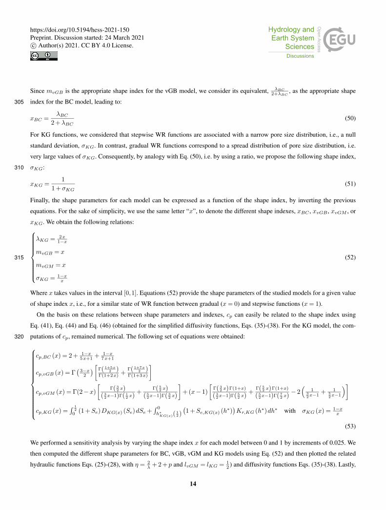
The hydraulic functions and diffusivity functions are plotted in Fig. 1 for the shape index value of 0.275, and their sensitivity330

upon each model’s shape index is shown in Fig. 2. For the sake of clarity, we plotted the relative hydraulic conductivity both

as functions of saturation degree, Kr (Se), and water pressure head, Kr (h∗), noting that these functions have distinct uses:

Kr (Se) defines the HC functions as a property of the soils, whereas Kr (h∗) is mostly used to compute sorptivity, e.g., as

in Eq. (13). Thus, Kr (h∗) has a similar role as the diffusivity function D∗ (Se), and the shapes and properties of these two

functions determine the values of the squared scaled sorptivity cp.335

The comparison between the hydraulic models (at the same shape index value) reveals some similarities and discrepancies

(Fig. 1). Three of the water retention models (vGB, vGM, KG) exhibit an inflection point with a continuous increase in

Se (h∗) over the whole interval (−∞,0] (Fig. 1a, “vGB”, “vGM”, and “KG”), while the BC model reaches the asymptote

Se = 1 at h∗ =−1 with full saturation for h∗ ≥−1 (Fig. 1a, “BC”). Despite that difference, the BC and vGB models exhibit

similar shapes (Fig. 1a, “BC” versus “vGB”). The vGM model exhibits a more progressive increase in Se (h∗) while remaining340

asymmetrically distributed across the inflection point (Fig. 1a, “vGM”). Lastly, the KG model exhibits an even more progressive

increase and a perfect symmetry around the inflection point (Fig. 1a, “KG”). The position of the inflection points depends on

the chosen hydraulic model. By construction, the inflection point is positioned at h∗ =−1 for the KG model. The others models

have inflection points positioned at larger abscises (in absolute values), with similar intermediate values for the BC and the

vGB models and the largest abscises for the vGM model (Fig. 1a).345

Regarding the relative hydraulic conductivity, the BC and vGB models have similar shapes for Kr (Se), with both typical

of power functions (Fig. 1b, “BC and “vGB”). In contrast, the vGM and KG models depict an inflection point, with larger

increase both at low saturation degrees and close to saturation compared to intermediate saturation degrees. In particular, these

two models exhibit a very large increase close to saturation whereas BC and vGB models have a gradual increase (Fig. 1b,

“vGM” and “KG” versus “BC” and “vGB”, close to Se = 1). This feature allows the vGM and KG models to simulate large350

drops in hydraulic conductivity close to saturation that are typical for certain soils. The functions Kr (h∗) are depicted in

Fig. 1c and combine the properties of the functions Kr (Se) and Se (h∗), as described depicted above. The function Kr (h∗)

exhibit similar shapes for BC and vGB models, with a quasi linear and sharp increase for h∗ ≤−1 followed by a plateau

(Fig. 1c, “BC” and “vGB”). The vGM and KG models exhibit a much more progressive increase, involving a much larger

range of water pressure heads. This feature is the most pronounced for the KG model. This more progressive increase reflects355

the more gradual WR functions, Se (h∗), as described in Fig. 1a combined with the drop in Kr (Se) that reaches unity only for

saturation degrees extremely close to unity (Fig. 1b).

15


10-3

100

103

106

0

1

0.2

0.4

0.6

0.8

0 10.2 0.4 0.6 0.80.1 0.3 0.5 0.7 0.910

-14

10-11

10-8

10-5

10-2

101

10-3

100

103

106

10-8

10-5

10-2

101

0 10.2 0.4 0.6 0.80.1 0.3 0.5 0.7 0.910

-8

10-5

10-2

101

(a) (b)

(c) (d)

Figure 1. Examples of water retention, Se (h∗) (a), relative unsaturated hydraulic, Kr (Se) (b) and Kr (h∗) (c), and diffusivity D∗ (Se)

functions (d) for the four hydraulic models: Brooks and Corey (BC), van Genuchten – Burdine (vGB), van Genuchten-Mualem (vGM), and

Kosugi (KG); the curves were plotted for a value of the shape index x of 0.275. The hydraulic parameters λBC , mvGM , mvGB , and σKG

were computed as a function of x using Eq. (52) with lvGM = lKG = 12

. The dashed line represents the "delta" model.

As for the WR and HC functions, the diffusivity functions exhibit close shapes for the BC and vGB models (Fig. 1d). The

BC model defines a concave shape with a finite maximum equal to λBC obtained at Se = 1, in line with the use of Eq. (35) at

Se = 1 (Fig. 1d, “BC”). In opposite, the vGB model diverts from the concave shape to tend towards infinity close to saturation,360

at Se = 1 (Fig. 1d, “vGB” versus “BC”). The vGB model defines a S shape that reflects the larger increases at both low and

high saturation degrees with lower increase at intermediate saturation degrees (Fig. 1d, “vGB”). The two other models, vGM

and KG, exhibit the same type of S shape with an infinite limit close to saturation (Fig. 1d, “vGM” and “KG”). Such infinite

limit spoils the numerical integration of Eqs. (23) for the determination of cp, requiring the use of the mixed formulation for

the KG models defined by Eqs. (47) and Eqs. (53).365

16


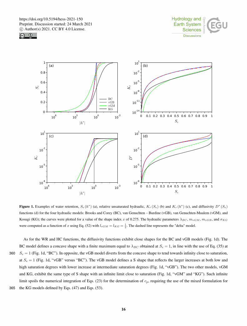
Varying the shape index changed the WRHC functions in an expected way (Fig. 2). For the WR functions, increasing the

shape index from 0 to 1 makes the shift from a gradual and moderate to an abrupt increase in saturation degree, respectively.

Values close to unity makes the WR functions close to a stepwise function corresponding to the Delta model (Fig. 2, 1st column,

arrows). As for the WR functions, the increase in the shape index put the curves Kr (h∗) close to stepwise functions (Fig. 2,

3rd column, arrows). For the BC model, we notice a decrease in Kr (h∗) for h∗ ≤−1 whereas Kr (h∗) remains equal to unity370

above (Fig. 2c, 3rd column). In opposite, for the vGB, vGM and KG models, the increase in the shape index has two antagonist

effects: a decrease of Kr (h∗) for h∗ ≤−1 followed by an increase for h∗ ≥−1 (Fig. 2g,k,n, 3rd column, arrows). Briefly,

as expected, the water retention and the relative hydraulic conductivity tend towards stepwise functions when the shape index

tends towards unity (Fig. 2, 1st and 3rd columns). This trend is less evident for the diffusivity functions (Fig. 2, 4th column).

These results show that, regardless of the selected model, increasing the shape index put the hydraulic functions closer to375

the Delta models that correspond to soils with narrow pore size distribution. In opposite, very small values of the shape index

ensure very gradual shapes for WR and HC functions. However, the results point at contrasting trends when the shape index is

decreased towards zero. It is clear that for the vGB and BC models, the relative hydraulic conductivity Kr (h∗) is not greatly

impacted close to h∗ = 0 (Fig. 2c,g). In opposite, for the vGM and KG models, Kr (h∗) tends towards zero in the vicinity of

h∗ = 0 (Fig. 2k,o, inverted arrows). Similarly, the dimensionless diffusivity D∗ (Se) tends towards zero over the whole interval380

[0,1] when the shape index tends towards zero (Fig. 2l,p, inverted arrows). Consequently, the features of Kr (h∗) and D∗ (Se)

functions presume very small values of the square scaled sorptivity for vGM and KG models, when the shape index tends

towards zero (see results below).

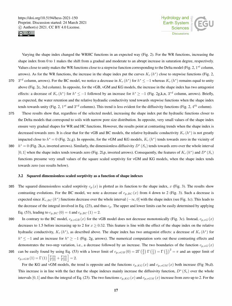
3.2 Squared dimensionless scaled sorptivity as a function of shape indexes

The squared dimensionless scaled sorptivity cp (x) is plotted as its function to the shape index, x (Fig. 3). The results show385

contrasting evolutions. For the BC model, we note a decrease of cp,BC (x) from 4 down to 2 (Fig. 3). Such a decrease is

expected since Kr,BC (h∗) functions decrease over the whole interval (−∞,0] with the shape index (see Fig. 1c). This leads to

the decrease of the integral involved in Eq. (23), and thus cp. The upper and lower limits can be easily determined by applying

Eq. (53), leading to cp,BC (0) = 4 and cp,BC (1) = 2.

In contrary to the BC model, cp,vGB (x) for the vGB model does not decrease monotonically (Fig. 3c). Instead, cp,vG (x)390

decreases to 1.5 before increasing up to 2 for x≥ 0.52. This feature is line with the effect of the shape index on the relative

hydraulic conductivity, Kr (h∗), as described above. The shape index has two antagonist effects: a decrease of Kr (h∗) for

h∗ ≤−1 and an increase for h∗ ≥−1 (Fig. 2g, arrows). The numerical computation sorts out these contrasting effects and

demonstrates the two-step variation, i.e., a decrease followed by an increase. The two boundaries of the function cp,vG (x)

can be easily found by using Eq. (53) with a lower limit of cp,vGB (0) = 2Γ(

32

)Γ(

12

)= Γ

(12

)2 = π and an upper limit of395

cp,vGB (1) = Γ(1)[

Γ(3)Γ(3) + Γ(4)

Γ(4)

]= 2.

For the KG and vGM models, the trend is opposite and the functions cp,KG (x) and cp,vGM (x) both increase (Fig 3b,d).

This increase is in line with the fact that the shape indexes mainly increase the diffusivity function, D∗ (Se) over the whole

intervals [0,1] and thus the integral of Eq. (23). The two functions cp,KG (x) and cp,vGM (x) increase from zero up to 2. For the

17


10-3

100

103

106

0

1

0.5

10-3

100

103

106

0

1

0.5

10-3

100

103

106

0

1

0.5

10-3

100

103

106

0

1

0.5

0 10.2 0.4 0.6 0.8

10-14

10-8

10-2

0 10.2 0.4 0.6 0.8

10-14

10-8

10-2

0 10.2 0.4 0.6 0.8

10-14

10-8

10-2

0 10.2 0.4 0.6 0.8

10-14

10-8

10-2

10-3

100

103

106

10-8

10-5

10-2

101

10-3

100

103

106

10-8

10-5

10-2

101

10-3

100

103

106

10-8

10-5

10-2

101

10-3

100

103

106

10-12

10-6

100

0 10.2 0.4 0.6 0.8

10-8

10-5

10-2

101

0 10.2 0.4 0.6 0.8

10-8

10-5

10-2

101

0 10.2 0.4 0.6 0.8

10-8

10-5

10-2

101

0 10.2 0.4 0.6 0.8

10-12

10-6

100

Figure 2. : Impact of the shape index, x, on the WRHC functions versus the selected hydraulic models: WR functions, Se (h∗) (1st column),

HC functions, Kr (Se) (2nd column) and Kr (h∗) (3rd column), and diffusivity function D∗ (Se) functions; Brooks and Corey (BC) (1st

row), van Genuchten – Burdine (vGB) (2nd row), van Genuchten-Mualem (vGM) (3rd row), and Kosugi (KG) models (4rd row); the arrows

indicate increasing values of the shape index x. The hydraulic parameters λBC , mvGM , mvGB , and σKG were computed as a function of x

using Eq. (52) with lvGM = lKG = 12

.

vGM model, the lower and upper limits can be demonstrated using Eq. (53) leading to cp,vGM (0) = 0 (see appendix A4) and400

cp,vGM (1) = Γ(1)[

Γ( 12 )

Γ( 12 ) +

Γ( 32 )

Γ( 32 )

]= 2. For KG hydraulic functions, the lower and upper limits were determined numerically,

leading also to 0 and 2, with null values over a large interval of shape index, i.e., [0,0.3] (Fig. 3b).

The four functions cp,BC (x), cp,vGB (x), cp,vGM (x), and cp,KG (x) all reach the value of 2 when the shape index approaches

unity, i.e., when the WR and HC functions tend towards stepwise functions. In fact, the value of cp (x) converges to the value

18


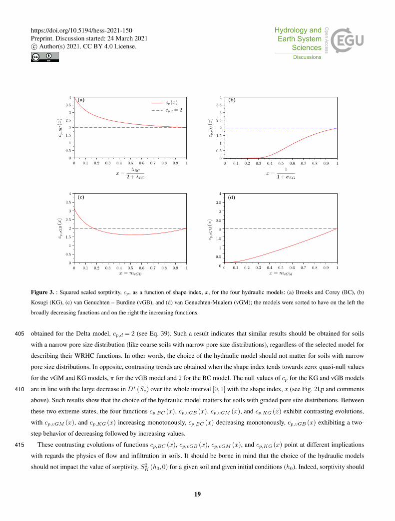
Figure 3. : Squared scaled sorptivity, cp, as a function of shape index, x, for the four hydraulic models: (a) Brooks and Corey (BC), (b)

Kosugi (KG), (c) van Genuchten – Burdine (vGB), and (d) van Genuchten-Mualem (vGM); the models were sorted to have on the left the

broadly decreasing functions and on the right the increasing functions.

obtained for the Delta model, cp,d = 2 (see Eq. 39). Such a result indicates that similar results should be obtained for soils405

with a narrow pore size distribution (like coarse soils with narrow pore size distributions), regardless of the selected model for

describing their WRHC functions. In other words, the choice of the hydraulic model should not matter for soils with narrow

pore size distributions. In opposite, contrasting trends are obtained when the shape index tends towards zero: quasi-null values

for the vGM and KG models, π for the vGB model and 2 for the BC model. The null values of cp for the KG and vGB models

are in line with the large decrease in D∗ (Se) over the whole interval [0,1] with the shape index, x (see Fig. 2l,p and comments410

above). Such results show that the choice of the hydraulic model matters for soils with graded pore size distributions. Between

these two extreme states, the four functions cp,BC (x), cp,vGB (x), cp,vGM (x), and cp,KG (x) exhibit contrasting evolutions,

with cp,vGM (x), and cp,KG (x) increasing monotonously, cp,BC (x) decreasing monotonously, cp,vGB (x) exhibiting a two-

step behavior of decreasing followed by increasing values.

These contrasting evolutions of functions cp,BC (x), cp,vGB (x), cp,vGM (x), and cp,KG (x) point at different implications415

with regards the physics of flow and infiltration in soils. It should be borne in mind that the choice of the hydraulic models

should not impact the value of sorptivity, S2K (h0,0) for a given soil and given initial conditions (h0). Indeed, sorptivity should

19


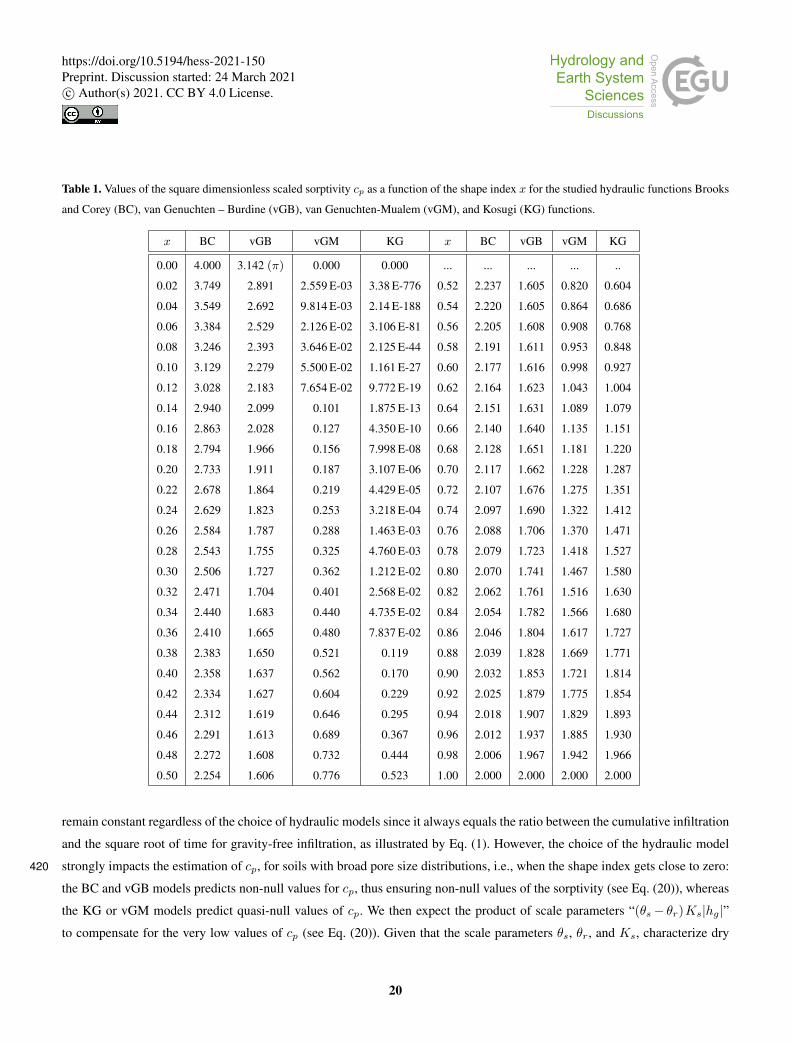
Table 1. Values of the square dimensionless scaled sorptivity cp as a function of the shape index x for the studied hydraulic functions Brooks

and Corey (BC), van Genuchten – Burdine (vGB), van Genuchten-Mualem (vGM), and Kosugi (KG) functions.

x BC vGB vGM KG x BC vGB vGM KG

0.00 4.000 3.142 (π) 0.000 0.000 ... ... ... ... ..

0.02 3.749 2.891 2.559 E-03 3.38 E-776 0.52 2.237 1.605 0.820 0.604

0.04 3.549 2.692 9.814 E-03 2.14 E-188 0.54 2.220 1.605 0.864 0.686

0.06 3.384 2.529 2.126 E-02 3.106 E-81 0.56 2.205 1.608 0.908 0.768

0.08 3.246 2.393 3.646 E-02 2.125 E-44 0.58 2.191 1.611 0.953 0.848

0.10 3.129 2.279 5.500 E-02 1.161 E-27 0.60 2.177 1.616 0.998 0.927

0.12 3.028 2.183 7.654 E-02 9.772 E-19 0.62 2.164 1.623 1.043 1.004

0.14 2.940 2.099 0.101 1.875 E-13 0.64 2.151 1.631 1.089 1.079

0.16 2.863 2.028 0.127 4.350 E-10 0.66 2.140 1.640 1.135 1.151

0.18 2.794 1.966 0.156 7.998 E-08 0.68 2.128 1.651 1.181 1.220

0.20 2.733 1.911 0.187 3.107 E-06 0.70 2.117 1.662 1.228 1.287

0.22 2.678 1.864 0.219 4.429 E-05 0.72 2.107 1.676 1.275 1.351

0.24 2.629 1.823 0.253 3.218 E-04 0.74 2.097 1.690 1.322 1.412

0.26 2.584 1.787 0.288 1.463 E-03 0.76 2.088 1.706 1.370 1.471

0.28 2.543 1.755 0.325 4.760 E-03 0.78 2.079 1.723 1.418 1.527

0.30 2.506 1.727 0.362 1.212 E-02 0.80 2.070 1.741 1.467 1.580

0.32 2.471 1.704 0.401 2.568 E-02 0.82 2.062 1.761 1.516 1.630

0.34 2.440 1.683 0.440 4.735 E-02 0.84 2.054 1.782 1.566 1.680

0.36 2.410 1.665 0.480 7.837 E-02 0.86 2.046 1.804 1.617 1.727

0.38 2.383 1.650 0.521 0.119 0.88 2.039 1.828 1.669 1.771

0.40 2.358 1.637 0.562 0.170 0.90 2.032 1.853 1.721 1.814

0.42 2.334 1.627 0.604 0.229 0.92 2.025 1.879 1.775 1.854

0.44 2.312 1.619 0.646 0.295 0.94 2.018 1.907 1.829 1.893

0.46 2.291 1.613 0.689 0.367 0.96 2.012 1.937 1.885 1.930

0.48 2.272 1.608 0.732 0.444 0.98 2.006 1.967 1.942 1.966

0.50 2.254 1.606 0.776 0.523 1.00 2.000 2.000 2.000 2.000

remain constant regardless of the choice of hydraulic models since it always equals the ratio between the cumulative infiltration

and the square root of time for gravity-free infiltration, as illustrated by Eq. (1). However, the choice of the hydraulic model

strongly impacts the estimation of cp, for soils with broad pore size distributions, i.e., when the shape index gets close to zero:420

the BC and vGB models predicts non-null values for cp, thus ensuring non-null values of the sorptivity (see Eq. (20)), whereas

the KG or vGM models predict quasi-null values of cp. We then expect the product of scale parameters “(θs− θr)Ks|hg|”to compensate for the very low values of cp (see Eq. (20)). Given that the scale parameters θs, θr, and Ks, characterize dry

20


(residual) or saturated states of the soil, these parameters are not expected to vary between the hydraulic models and are

supposed fixed. Consequently, only the scale parameters for water pressure head, |hg|, is expected to compensate for the very425

low values of cp when the vGM and KG models are used. We conclude that the value of |hg| must tends towards infinite when

the shape index tends towards zero for these two models. For KG models, such relation |hKG| xKG is related to the relation

|hKG| σKG since xKG = (1 +σKG)−1. Our statements imply that very larges values of σKG(xKG→ 0) should be associated

to very larges values of |hKG|, i.e., to very small pore radius. In other words, fine (coarse) soils with small (large) pores

should have broad (narrow) pore size distributions. These considerations are in line the previous studies on KG by Pollacco430

et al. (2013) (see Fig. 1 of their paper), and Fernández-Gálvez et al.. These authors even related the pore radius of soil to

the standard deviation of pore size distribution with a strongly decreasing function. Similar trends relating to some extent a

relation between pore mean and pore standard deviation should also apply to vGM model given our findings (and to avoid null

sorptivity for soils with broad pore size distributions). More investigations are needed to verify for real soils such link between

average pore size and standard deviations. More investigations are also needed to guide on the proper choice of the hydraulic435

models as a function of the type of soil, as already suggested by Fuentes et al. (1992). These aspects will be the subject of a

specific study.

Regarding the numerical accuracy of computed values of cp, we used analytical formulations for the BC, vGB and vGM

models as detailed in Eqs. (53). These values are expected to be perfect without any error since their correspond to the ap-

plication of exact analytical formulations. Instead, we used the mixed numerical formulation defined by Eqs. (53) for the KG440

model that relies on the numerical integration of the hydraulic conductivity or diffusivity functions. In that case, the numerical

integration may bring some numerical errors. The mixed form Eq. (47) was designed to minimize numerical indetermination

and uncertainty. Such formulation was applied to the other models (BC, vGB and vGM) and the resulting values were com-

pared against the analytical formulations (considered as the benchmark). A perfect agreement was obtained (errors < 1%), thus

validating the numerical mixed formulation and making the authors very confident on the values tabulated in Table 1. Note that445

the promotion of the numerical mixed formulation and the study of its uncertainty will be the subject of another study.

3.3 Upscaling sorptivity S2K (h0,0) from cp

In this section, we elaborate on the use of Eq. (22) for the easy and straightforward computation of S2K (h0,0) from the

tabulated values of cp (Table 1). The proposed scaling procedure Eq. (22) allows the computation of S2K (h0,0) given initial

hydric conditions (water contents or the water pressure heads), hydraulic shape and scale parameters, and specific hydraulic450

models selected among the studied hydraulic models Eqs. (7)-(10):

1. Use the shape parameter (λBC , mvGB , mvGM or σKG to compute the related shape index, x, considering the following

definitions: xvGB =mvGB , xvGM =mvGM , xKG = 1/(1 +σKG), and xBC = λBC2+λBC

.

2. Choose in Table 1 the value of cp corresponding to the shape index, x, and the chosen WRHC functions.

3. Consider or compute the initial water content θ0 or θ (h0) depending on the observation for the description of the initial455

condition (either θ0 or h0).

21


4. Compute the related hydraulic conductivity, K0 =K (θ0), using the HC function.

5. Compute the correcting factors Rθ = θs−θ0θs−θr and RK = Ks−K0

Ks.

6. Compute the scaled air-entry water pressure head: |h∗a|= |hahg |

7. Compute the square scaled sorptivity S2∗K (h∗0,0) =RKRθ (cp− 2|h∗a|) + 2Rθ|h∗a|460

8. Upscale to derive the square sorptivity: S2K (h0,0) = S2∗

K (h∗0,0) (θs− θr)Ks|hg|

As an illustrative example, let consider the case of a loamy soil submitted to water saturation with a slightly positive water

pressure head at the surface (h1 = 0) and an initial water pressure head of h0 =−10 m (dry conditions). The loamy soil has

the features of “loam” as defined in the database of Carsel and Parrish (1988). Its WRHC functions are described by the vGM

model, with the following shape and scale parameters: θr = 0.078, θs = 0.43, hg =−277 mm, and Ks = 2.88 10−3 mm s−1,465

nvGM = 1.56, and lvGM = 0.5. The application of the step-by-step procedure gives the following results:

1. Shape index: x=mvGM = 1− 1/nvGM leading to x= 0.359

2. Corresponding value of cp: cp = 0.480, given Table 1 (“vGM model” column, x= 0.36)

3. Initial water content: computed from the initial water pressure head of -10 m using vGM-WR function, i.e., Eqs. (9):

θ0 = 0.125.470

4. Initial hydraulic conductivity: computed from the initial water content using vGM-HC function,i.e., Eqs. (9):

K0 = 1.8710−9 mm s−1.

5. Corresponding correction factors: Rθ = θs−θ0θs−θr and RK = Ks−K0

K0, leading to:

Rθ = 0.865 and RK = 1.000

6. Air-entry water pressure head: no air-entry water pressure head, consequently, |h∗a|= 0475

7. Square scaled sorptivity: S2∗K (h∗0,0) =RKRθcp leading to:

S2∗K (h∗0,0) = 0.416

8. Sorptivity: S2K (h0,0) = S2∗

K (h∗0,0)(θs− θr)Ks|hg|, leading to:

S2K (h0,0) = 0.117 mm2 s−1, and SK (h0,0) = 0.342 mms−

12

To check the accuracy of the proposed approximation, we computed the nominal value of the sorptivity, using the regular480

Eq. (2). We found a very close value, with less than 0.5% relative error, demonstrating the accuracy of the proposed scaling

procedure Eq. (22).

As a second illustrative example, we consider the computation of sorptivity for the case of BC model, for the same conditions.

The difference with the previous case is that the BC model has a non-null air-entry water pressure head, inducing a non-null

22


saturated sorptivity. We consider the same loamy soil with the following parameters for BC model: r = 0.078, θs = 0.43,485

hg =−277 mm, and Ks = 2.88 10−3 mm s−1, with a value of λBC = 0.56. λBC was deduced from the previous value of

n= 1.56 considering the usual relation λ=mn, as suggested by Haverkamp et al. (2005). The application of the proposed

procedure leads to the following computations:

1. Shape index: xBC = λBC/(2 +λBC) leading to a value of xBC = 0.219

2. Corresponding value of cp: cp = 2.678 (see Table 1, “BC model” column for xBC = 0.22)490

3. Initial water content: computed from the initial water pressure head of -10 m using BC-WR function, i.e., Eqs. (7):

θ0 = 0.125.

4. Initial hydraulic conductivity: computed from the initial water content using BC-HC function, i.e., Eqs. (7):

K0 = 3.34210−9 mm s−1.

5. Corresponding correction factors: Rθ = θs−θ0θs−θr and RK = Ks−K0

K0, leading to:495

Rθ = 0.866 and RK = 1.000

6. Air-entry water pressure head: significant air-entry water pressure head, with, |hBC = ha| and |h∗a|= 1

7. Square scaled sorptivity: S2∗K (h∗0,0) =RKRθ (cp− 2|h∗a|) +−2Rθ |h∗a| leading to:

S2∗K (h∗0,0) = 2.318

8. Sorptivity: S2K (h0,0) = S2∗

K (h∗0,0)(θs− θr)Ks|hg|, leading to:500

S2K (h0,0) = 0.651mm2 s−1, and SK (h0,0) = 0.806 mm s−

12

Again, the exact value of sorptivity was estimated using the accurate Eq. (3) and lead to a similar value with a relative

error of 1‰. Note that, in this case, due to the non-null air-entry water pressure head, Eq. (3) must be employed instead of

Eq. (2) for the determination of the targeted value of sorptivity. The two preceding applications illustrated the accuracy of the

proposed scaling procedure Eq. (20) for the two cases of hydraulic functions with and without air-entry water pressure heads.505

Equation (20) proved appropriate and very accurate for the determination of the sorptivity, S2K (h0,0).

It must be noted that the proposed scaling procedure applies only for dry initial state. Indeed, Haverkamp et al. (2005)

stated that their approximation Eq. (15) was ensured only when θ0 ≤ 14 θs. For fine soils, even a small initial water pressure

head may cause θ0 >14 θs, which may spoil the proposed scaling procedure. To illustrate this point, we investigated the case

of the silty clay soil, as defined by Carsel and Parrish (1988). This soil is defined for the following parameters: θr = 0.07,510

θs = 0.36, hg =−2000 mm, and Ks = 5.555 10−5 mm s−1, n= 1.09, and l = 0.5. Considering the same value for the initial

water pressure head, i.e., h0 =−10 m, the initial water content is θ0 = 0.318; which exceeds 14θs. The application of the

scaling procedure lead to an estimated sorptivity of 0.0475 mm s−12 , whereas the targeted sorptivity computed with Eq. (2)

was 0.0127 mm s−12 . Such error corresponds to an overestimation by a factor of 2.73. Thus, we advise that the user verify that

θ0 ≤ 14 θs before using the proposed scaling procedure.515

23


4 Conclusions

The proper estimation of sorptivity is crucial to understand and model water infiltration into soils. However, its estimation

may be complicated, requiring complicated algebraic derivations and exhibiting potential numerical shortcomings when using

Eq. (2) or Eq. (3). In this study, we present a new scaling procedure for simplifying the computation of sorptivity for the case

of zero water pressure head imposed at surface and dry initial state (θ0 ≤ 14θs). We based our approach on the combination and520

adaptation of the scaling procedure proposed by Ross et al. (1996) and the approximation proposed by Haverkamp et al. (2005).

We then obtain a simple relation that relates the square sorptivity to the product of the square scaled sorptivity, referred to as

cp, the product of scale parameters and two correction factors that account for the initial conditions, (i.e., initial water content

and hydraulic conductivity). The value of the square scaled sorptivity cp was computed either analytically, when feasible, or

numerically, for four famous sets of hydraulic models: Brooks and Corey, van Genuchten – Mualem, van-Genuchten – Burdine525

and Kosugi models. The values of cp were tabulated as function of specific shape indexes representing similar states of WR

functions (well-graded versus stepwise shapes) between hydraulic models. The proposed scaling procedure is very easy of use.

Once a given hydraulic model is selected with related shape and scale parameters, the procedure steps are easy to perform:

computation of the shape index from the shape parameters, reading of the corresponding value of cp in Table 1, computation

of the correction factors (ratios in hydraulic conductivity and water contents, RK and Rθ), computation of the square scaled530

sorptivity from cp and these correction factors, and, lastly, upscaling by multiplying with the scale parameters. All these steps

are easy to conduct and straightforward. Illustrative examples are proposed at the end of this study and the accuracy of the

proposed scaling procedure is clearly demonstrated (with errors less than 1%), provided that the initial water content fulfills

the conditions: (θ0 ≤ 14θs).

In addition to providing a straightforward method for the determination of sorptivity, this study brings very interesting535

findings on the square scaled sorptivity cp and its dependency upon the shape index, x and the chosen hydraulic models.

The results show that the function cp (x) strongly depends on the hydraulic model selected for the WRHC curves. If all the

functions cp (x) converge for the same value, i.e., 2, close to x= 1 (stepwise WR functions – narrow pore size distribution),

they strongly divert close to x= 0 (graded WR functions – broad pore size distribution), with values of 0 for vGM and KG

models versus 3 - 4 for the vGB and BC models. However, the sorptivity should remain the same regardless of the selected540

hydraulic model: one soil submitted to peculiar initial conditions, one single sorptivity. Consequently, the contrast of scaled

sorptivity must be compensated by a contrast in scale parameters. However, among scale parameters, the residual and saturated

water contents and the saturated hydraulic conductivity cannot be changed between models, since they characterize the dry and

saturated states of the same soil. Consequently, the value of the scale parameter hg must be the one to compensate. Previous

studies on the Kosugi model have already hypothesized a strong relation between the scale parameter hKG and the standard545

deviation σKG (Pollacco et al., 2013). In other words, the scale parameter hKG should be parametrized as a function of the

shape parameter σKG, to get plausible WRHC functions and estimates of sorptivity. We may also expect the same link between

the scale parameter hg,vGM and the shape parameter mvGM to avoid unphysical scenarios and null sorptivity. However, such

hypothesis has never been suggested and requires further investigations. These results show the need to better understand the

24


mathematical properties of the hydraulic models, including the links between shape and scale parameters, and to better relate550

these properties to the physical processes of water infiltration into soils (Fuentes et al., 1992).

In addition to the proposed scaling procedure, this study gave the opportunity to derive analytically the scaled sorptivity for

the three models, BC, vGB and vGM, thus confirming the expressions provided by previous studies. For the vGM model, the

analytical derivation is brand new and had never been proposed before. Its use if of great interest and could be implemented

into soil hydraulic characterization methods. For instance, additional BEST methods could be developed ob the basis of the555

use of the proposed formulations for square scaled sorptivity to relate sorptivity to shape and scale parameters. In more details,

the prior estimation of shape parameters allows the determination of the parameter cp using Eq. (45). Then, the estimation of

saturated hydraulic conductivity, and sorptivity allows the determination of scale parameter hg once cp is determined. A similar

procedure may be proposed for the vGM model, using the Eq. (46) that defines the parameter cp to the shape parametermvGM .

The development of BEST method for the specific vGM hydraulic model, that is much more used than the vGB model, will560

be the subject of further investigations. It would also be interesting to derive somehow the residual water content, and not to

assume it to be equal to zero as it might alter the shape of the soil water retention function. The use of the scaled sorptivity for

these purposes are the subject of ongoing studies.

Code availability. Note all computations were done using Scilab free software. The scripts for the computation of Eqs. (25)-(28) for the

computation of WRHC functions, Eqs. (35)-(38) for the computation of the dimensionless diffusivity, and Eqs. (35)-(38) for the computation565

of the cp parameter can be downloaded online: https://zenodo.org/record/4587160 (Lassabatere, 2021).

Appendix A: Dimensionless hydraulic diffusivity functions, D∗(Se)

In the appendices, for the sake of clarity the notations of the shape parameters were simplified to λ, m, n, σ, in order to avoid

heavy equations. The dimensionless diffusivity functions were derived from their definition D∗ (Se), applying D∗ (Se) =

Kr (Se) dh∗

dSe. This task requires first to derive the inverse functions for the dimensionless water retention curves. The following570

equations can be easily found through usual algebraic developments:

h∗BC (Se) =−S−1λ

e (A1)

h∗vGB (Se) =−(S− 1m

e − 1) 1n

with m= 1− 2n

(A2)

h∗vGM (Se) =−(S− 1m

e − 1) 1n

with m= 1− 1n

(A3)

h∗KG (Se) =−e√

2σerfc−1(2Se) (A4)575

25


where erfc−1 is the inverse function of the complementary error function. These functions can be differentiated to define their

relative derivatives, dh∗

dSe:

dh∗BCdSe

(Se) =1λS− 1λ−1

e (A5)

dh∗vGBdSe

(Se) =1−m2m

S− 1+m

2me

(1−S

1me

)−m+12

(A6)

dh∗vGMdSe

(Se) =1−mm

S− 1m

e

(1−S

1me

)−m(A7)580

dh∗KGdSe

(Se) =√

2πσe(erfc−1(2Se))2

+√

2σerfc−1(2Se) (A8)

The differentiation of the function h∗KG involves the following usual rules of differentiation (f og)′= f

′og · g′ and

(f−1

)′=

1f ′ of−1 , considering bijective functions. We also use the usual derivative of the function erf function, erf

′(x) = 2√

πe−x

2, and

the relation between erfc and erf functions, erfc(x) = 1− erf(x).

The derivatives dh∗

dSecan now be multiplied with the hydraulic conductivity:585

Kr,BC (Se) = S ηe (A9)

Kr,vGB (Se) = S ηe (A10)

Kr,vGM (Se) = S le

(1− 2

(1−S

1me

)m+(

1−S1me

)2m)

(A11)

Kr,KG (Se) = S le

(12erfc

(erfc−1 (2Se) +

σ

2

))2

(A12)

Note that for the hydraulic conductivity function of vGM model, Kr,vGM , we distributed the terms according to (a+ b)2 =590

a2 + 2ab+ b2. The multiplication of Eqs. (A5)-(A8) with the expressions of relative conductivity Eq. (A9)-(A12) lead to the

following expressions of dimensionless diffusivity:

D∗BC (Se) = 1λS

η−( 1λ+1)

e

D∗vGB (Se) = 1−m2m S

η− 1+m2m

e

(1−S

1me

)− 1+m2

D∗vGM (Se) = 1−mm S

l− 1m

e

((1−S

1me

)−m+(

1−S1me

)m− 2)

D∗KG (Se) = 12

√π2σS

le

(erfc

(erfc−1 (2Se) + σ√

2

))2

e(erfc−1(2Se))2

+√

2σerfc−1(2Se)

(A13)

These equations, Eqs. (A13), correspond to the expressions of Eqs. (30)-(33). Afterwards, the combination with the capillarity

model Eq. (34) leads to Eqs. (35)-(38).595

26


Appendix B: Analytical developments for cp parameter

B1 Parameter cp for BC model

For the BC model, we need to account for the air entry pressure, h∗a =−1. We remind that by convention, the scale parameters

for water pressure head, hBC is equalled to the air-entry water pressure head, ha. We then use the equation Eq. (23) with |h∗a|=1. Then, the first part

∫ 1

0(1 +Se)D∗BC (Se)dSe can be integrated analytically given that the hydraulic diffusivity D∗BC (Se)600

obeys a power law. The following developments can be done:

cp,BC =

1∫

0

(1 +Se)D∗BC (Se)dSe + 2 |h∗a|

=

1∫

0

(1 +Se)D∗BC (Se)dSe + 2 (B1)

1∫

0

(1 +Se)D∗BC (Se)dSe =

1∫

0

D∗BC (Se)dSe +

1∫

0

SeD∗BC (Se)dSe

=

1∫

0

1λSη−( 1

λ+1)e dSe +

1∫

0

1λSeS

η−( 1λ+1)

e dSe

=1λ

1∫

0

Sη−( 1

λ+1)e dSe +

1∫

0

Sη− 1

λe dSe

=1λ

(1

η− 1λ

+1

η− 1λ + 1

)

=1

ηλ− 1+

1ηλ+λ− 1

(B2)

The final expression can be easily computed by combining Eqs. (B1) and Eqs. (B2):605

cp,BC (λ,η) =1

ηλ− 1+

1ηλ+λ− 1

+ 2 (B3)

The concatenation of the Eq. (B3) with the capillary model, Eq.( 34), leads to the following final expression:

cp,BC (λ) = 2 +1

3λ+ 1+

14λ+ 1

(B4)

These development demonstrate the equations proposed for cp for the BC model, i.e., Eqs. (40)-(41). This demonstration is in

line with Varado et al. (2006).610

27


B2 Parameter cp for vGB model

For vGB model, and the remaining models, there is no air-entry water pressure head, h∗a = 0, leading to:

cp,vGB =

1∫

0

(1 +Se)D∗vGB (Se)dSe + 2 |h∗a|

=

1∫

0

(1 +Se)D∗vGB (Se)dSe (B5)

Then, the integral∫ 1

0(1 +Se)D∗vGB (Se)dSe can be decomposed into well-known integrals:

cp,vGB (m,η) =

1∫

0

(1 +Se)D∗vGB (Se)dSe

=

1∫

0

D∗vGB (Se)dSe +

1∫

0

SeD∗vGB (Se)dSe

=

1∫

0

1−m2m

Sη− 1+m

2me

(1−S

1me

)− 1+m2dSe +

1∫

0

Se1−m2m

Sη− 1+m

2me

(1−S

1me

)− 1+m2dSe

=1−m2m

1∫

0

Sη− 1+m

2me

(1−S

1me

)− 1+m2dSe +

1∫

0

SeSη− 1+m

2me

(1−S

1me

)− 1+m2dSe

1−m2m

1∫

0

Sη− 1+m

2me

(1−S

1me

)− 1+m2dSe +

1∫

0

Sη+1− 1+m

2me

(1−S

1me

)− 1+m2dSe

=1−m2m

1∫

0

(S

1me

)mη− 1+m2(

1−S1me

)− 1+m2dSe +

1∫

0

(S

1me

)mη+m− 1+m2(

1−S1me

)− 1+m2dSe

(B6)615

The change of variable y = S1me provides the following expressions:

cp,vGB (m,η) =1−m

2

1∫

0

ymη+m2 − 3

2 (1− y)−m+1

2 dy+1−m

2

1∫

0

ymη+ 3m2 − 3

2 (1− y)−m+1

2 dy (B7)

We can recognize in equation the beta function B and use its following properties (assuming x > 0 and y > 0):

B (x,y) =

1∫

0

tx−1 ty−1dt

=Γ(x)Γ(y)Γ(x+ y) (B8)

28


Where the Γ function is already defined by Eq. (43): Γ(z) =∫ +∞

0tz−1 e−tdt (z > 0). Then, the parameter cp,vGB can be620

expressed as follows:

cp,vGB (m,η) =1−m

2B

(mη+

m

2− 1

2,1−m

2

)+

1nB

(mη+

3m2− 1

2,1−m

2

)

=1−m

2Γ(

1−m2

)(Γ(mη+ m

2 − 12

)

Γ(mη)+

Γ(mη+ 3m

2 − 12

)

Γ(mη+m)

)

= Γ(

3−m2

)(Γ(mη+ m

2 − 12

)

Γ(mη)+

Γ(mη+ 3m

2 − 12

)

Γ(mη+m)

)

(B9)

The last equation uses the fact that Γ(z+1) = zΓ(z). The Eq. (B9) corresponds to the equation suggested by Haverkamp et al.

(2005), considering m= 1− 2n :

cp,vGB (n,m,η) = Γ(

1 +1n

)(Γ(mη− 1

n

)

Γ(mη)+

Γ(mη+m− 1

n

)

Γ(mη+m)

)(B10)625

Note that the proposed simplification using the beta function, Eq. (B9) requires that mη+ m2 − 1

2 > 0, which is quite evident

since m< 1. When Eq. (B9) is combined with capillary model, i.e., Eq. (34), the expression becomes:

cp,vGB (m) = Γ(

3−m2

)(Γ(

1+5m2

)

Γ(1 + 2m)+

Γ(

1+7m2

)

Γ(1 + 3m)

)(B11)

The expressions of the parameter cp for the vGB model are accurately demonstrated, leading to Eqs. (42) and (44).

B3 Parameter cp for vGM model630

For the vGM model, the same equation Eq. (B5) applies and can be cut into two parts:

cp,vGM (m,l) =

1∫

0

(1 +Se)D∗vGM (Se)dSe

=

1∫

0

D∗vGM (Se)dSe

︸︷︷︸A

+

1∫

0

SeD∗vGM (Se)dSe

︸︷︷︸B

(B12)

For the sake of clarity, we demonstrate separately the simplifications of the two terms A and B:

A =1−mm

∫ 1

0

Sl− 1

me

((1−S

1me

)−m+(

1−S1me

)m− 2)dSe

=1−mm

(∫ 1

0

Sl− 1

me

(1−S

1me

)−mdSe +

∫ 1

0

Sl− 1

me

(1−S

1me

)mdSe− 2

∫ 1

0

Sl− 1

me dSe

)

=1−mm

(∫ 1

0

(S

1me

)ml−1(1−S

1me

)−mdSe +

∫ 1

0

(S

1me

)ml−1(1−S

1me

)mdSe− 2

∫ 1

0

Sl− 1

me dSe

)(B13)

29


The last term of A can be simplified easily:635

1∫

0

Sl− 1

me dSe =

1∫

0

Sl− 1

me dSe =

[Sl− 1

m+1e

l− 1m + 1

]1

0

=m

(l+ 1)m− 1(B14)

For the two first, terms, we use the same change of variable y = S1me as above to transform the integrals, leading to:

A = (1−m)

1∫

0

yml+m−2 (1− y)−m dy+

1∫

0

yml+m−2 (1− y)m dy− 2(l+ 1)m− 1

(B15)

In this case, we need to assume that ml+m− 2>−1, i.e. m> 1l+1 to use the beta function. Such a condition corresponds to

m> 23 , for the by-default value of l = 1

2 . The two first integrals can then be replaced using the beta and the gamma functions,640

leading to the final expression for part A of cp:

A = (1−m)(B (m(l+ 1)− 1,1−m) +B (m(l+ 1)− 1,1 +m)− 2

(l+ 1)m− 1

)

= (1−m)(

Γ(m(l+ 1)− 1)Γ(1−m)Γ(ml)

+Γ(m(l+ 1)− 1)Γ(1 +m)

Γ(m(l+ 2))− 2

(l+ 1)m− 1

)(B16)

By analogy, the following developments come out for parameter B:

B = (1−m)(

Γ(m(l+ 2)− 1)Γ(1−m)Γ(ml+m)

+Γ(m(l+ 2)− 1)Γ(1 +m)

Γ(m(l+ 3))− 2

(l+ 2)m− 1

)(B17)

The simplification for B is valid as soon as m> 12+l , which is the case since we suppose that m> 1

1+l . After rearranging645

terms, the following expressions comes out for the dimensionless sorptivity:

cp,vGM (m,l) = Γ(2−m)

(Γ(m(l+ 1)− 1)

Γ(ml)+

Γ(m(l+ 2)− 1)Γ(1−m)

Γ(ml+m)

)+ (1−m)

[(Γ(m(l+ 1)− 1)Γ(1 +m)

Γ(m(l+ 2))+

Γ(m(l+ 2)− 1)Γ(1 +m)

Γ(m(l+ 3))

)− 2

(1

(l+ 1)m− 1+

1

(l+ 2)m− 1

)](B18)

cp,vGM (m,l) = Γ(2−m)

(Γ(m(l+ 1))

(m(l+ 1)− 1) Γ(ml)+

Γ(m(l+ 2))

(m(l+ 2)− 1) Γ(ml+m)

)+ (1−m)

[(Γ(m(l+ 1)− 1) Γ(1 +m)

Γ(m(l+ 2))+

Γ(m(l+ 2)− 1) Γ(1 +m)

Γ(m(l+ 3))

)− 2

(1

(l+ 1)m− 1+

1

(l+ 2)m− 1

)](B19)

Note that, as stated above, that equation theoretically should apply only for the case of m> 11+l , which is quite restrictive.650

However, thanks to the analyticity of the functions involved in the expression, this equality remains valid for m> 11+l and can

be considered for any value of m ∈ [0,1] provided that m 6= 11+l and m 6= 1

2+l . The Eq. (B19) demonstrates the Eqs. (42). The

combination of these equations with the capillary model Eq. (34) leads to Eqs. (46).

30


Author contributions. L.L.: established the question, performed the analytical developments, computed the numerical results, provided the

first draft of the manuscript. P.-E.P. performed the analytical developments and verified the numerical results. D.Y., B.L., D.M.-F., S.d.P. and655

M.R. verified parts of the developments and numerical computations. J. P. and J. F.-G. helped for the use of the Kosugi model. R.D.S. and

M.A.N. helped for the editing and the presentation of the results, in particular the writing of the application of the proposed approach for

end-users. All the authors contributed to the editing of the manuscript.

Competing interests. No competing interest to declare.

Acknowledgements. This work was performed within the INFILTRON project supported by the French National Research Agency (ANR-660

17-CE04-010).

31


References

Angulo-Jaramillo, R., Bagarello, V., Iovino, M., and Lassabatere, L.: Infiltration measurements for soil hydraulic characterization, Infiltration

Measurements for Soil Hydraulic Characterization, https://doi.org/10.1007/978-3-319-31788-5, 2016.

Angulo-Jaramillo, R., Bagarello, V., Di Prima, S., Gosset, A., Iovino, M., and Lassabatere, L.: Beerkan Estimation of Soil Transfer parameters665

(BEST) across soils and scales, Journal of Hydrology, 576, 239–261, https://doi.org/10.1016/j.jhydrol.2019.06.007, 2019.

Bagarello, V., Di Prima, S., and Iovino, M.: Comparing alternative algorithms to analyze the beerkan infiltration experiment, Soil Science

Society of America Journal, 78, 724–736, https://doi.org/10.2136/sssaj2013.06.0231, 2014.

Braud, I.: European Journal of Soil Science, 56, 361, 2005.

Brooks, R. and Corey, A.: Hydraulic Properties of Porous Media, Hydrology Papers, Colorado State University, 1964.670

Carsel, R. F. and Parrish, R. S.: Developing joint probability distributions of soil water retention characteristics, Water Resources Research,

24, 755–769, https://doi.org/10.1029/WR024i005p00755, 1988.

Cook, F. and Minasny, B.: Sorptivity of Soils, in: Encyclopedia of Earth Sciences Series, pp. 824–826, https://doi.org/10.1007/978-90-481-

3585-1_161, 2011.

Fernández-Gálvez, J., Pollacco, J., Lassabatere, L., Angulo-Jaramillo, R., and Carrick, S.: A general Beerkan Estimation of Soil Transfer675

parameters method predicting hydraulic parameters of any unimodal water retention and hydraulic conductivity curves: Application to the

Kosugi soil hydraulic model without using particle size distribution data, 129, 118–130.

Fuentes, C., Haverkamp, R., and Parlange, J.-Y.: Parameter constraints on closed-form soil water relationships, Journal of hydrology, 134,

117–142, 1992.

Haverkamp, R., Leij, F. J., Fuentes, C., Sciortino, A., and Ross, P.: Soil water retention, Soil Science Society of America Journal, 69,680

1881–1890, 2005.

Hillel, D.: Environmental soil physics: Fundamentals, applications, and environmental considerations., Academic press.

Kosugi, K.: Lognormal Distribution Model for Unsaturated Soil Hydraulic Properties, Water Resources Research, 32, 2697–2703,

https://doi.org/https://doi.org/10.1029/96WR01776, 1996.

Kosugi, K. and Hopmans, J.: Scaling water retention curves for soils with lognormal pore-size distribution, Soil Science Society of America685

Journal, 62, 1496–1505, 1998.

Lassabatere, L.: Scilab script for sorptivity, https://doi.org/10.5281/zenodo.4587160, 2021.

Lassabatere, L., Angulo-Jaramillo, R., Soria Ugalde, J. M., Cuenca, R., Braud, I., and Haverkamp, R.: Beerkan estima-

tion of soil transfer parameters through infiltration experiments—BEST, Soil Science Society of America Journal, 70, 521,

https://doi.org/10.2136/sssaj2005.0026, 2006.690

Lassabatere, L., Angulo-Jaramillo, R., Soria-Ugalde, J., Šimunek, J., and Haverkamp, R.: Numerical evaluation of a set of analytical infiltra-

tion equations, Water Resources Research, 45, https://doi.org/10.1029/2009WR007941, 2009.

Lassabatere, L., Yilmaz, D., Peyrard, X., Peyneau, P., Lenoir, T., Šimunek, J., and Angulo-Jaramillo, R.: New analytical model for cumulative

infiltration into dual-permeability soils, Vadose Zone Journal, 13, 1–15, https://doi.org/10.2136/vzj2013.10.0181, 2014.

Lassabatere, L., Di Prima, S., Bouarafa, S., Iovino, M., Bagarello, V., and Angulo-Jaramillo, R.: BEST-2K Method for Char-695

acterizing Dual-Permeability Unsaturated Soils with Ponded and Tension Infiltrometers, Vadose Zone Journal, 18, 180 124,

https://doi.org/10.2136/vzj2018.06.0124, publisher: John Wiley & Sons, Ltd, 2019.

32


Mualem, Y.: A new model for predicting the hydraulic conductivity of unsaturated porous media, Water Resources Research, 12, 513–522,

1976.

Parlange, J.-Y.: On Solving the Flow Equation in Unsaturated Soils by Optimization: Horizontal Infiltration, Soil Science Society Of America700

Journal, 39, 415–418, 1975.

Philip, J. R.: The theory of infiltration: 2. the profile at infinity, Soil Science, 83, 257–264, 1957.

Pollacco, J., Nasta, P., Soria-Ugalde, J., Angulo-Jaramillo, R., Lassabatere, L., Mohanty, B., and Romano, N.: Reduction

of feasible parameter space of the inverted soil hydraulic parameter sets for Kosugi model, Soil Science, 178, 267–280,

https://doi.org/10.1097/SS.0b013e3182a2da21, 27, 2013.705

Ross, P., Haverkamp, R., and Parlange, J.-Y.: Calculating parameters for infiltration equations from soil hydraulic functions, Transport in

porous media, 24, 315–339, 1996.

Triadis, D. and Broadbridge, P.: The Green–Ampt limit with reference to infiltration coefficients, Water Resources Research, 48, WR011 747,

https://doi.org/10.1029/2011WR011747, 2012.

van Genuchten, M.: A closed-form equation for predicting the hydraulic conductivity of unsaturated soils., Soil science society of America710

journal, 44, 892–898, 1980.

Varado, N., Braud, I., Ross, P. J., and Haverkamp, R.: Assessment of an efficient numerical solution of the 1D Richards’ equation on bare

soil, Journal of Hydrology, 323, 244–257, 2006.

Yilmaz, D., Lassabatere, L., Angulo-Jaramillo, R., Deneele, D., and Legret, M.: Hydrodynamic characterization of basic oxygen furnace slag

through an adapted best method, Vadose Zone Journal, 9, 107–116, https://doi.org/10.2136/vzj2009.0039, 2010.715

Šimunek, J., Jarvis, N. J., van Genuchten, M. T., and Gärdenäs, A.: Review and comparison of models for describing non-equilibrium and

preferential flow and transport in the vadose zone, Journal of Hydrology, 272, 14–35, 2003.

33


Scaling procedure for straightforward computation of ...

Documents

Transcript of Scaling procedure for straightforward computation of ...