1

Scaling Laws of Multicast Capacity forPower-Constrained Wireless Networks under

Gaussian Channel ModelCheng Wang, Changjun Jiang, Member, IEEE, Xiang-Yang Li, Senior Member, IEEE,

Shaojie Tang, Yuan He, Member, IEEE, Xufei Mao, and Yunhao Liu, Senior Member, IEEE

Abstract—In this paper, we study the asymptotic networking-theoretic multicast capacity bounds for random extended networks (REN)under Gaussian channel model, in which all wireless nodes are individually power-constrained. During the transmission, the powerdecays along path with attenuation exponent α > 2. In REN, n nodes are randomly distributed in the square region of side length

√n.

There are ns randomly and independently chosen multicast sessions. Each multicast session has nd + 1 randomly chosen terminals,including one source and nd destinations. By effectively combining two types of routing and scheduling strategies, we analyze theasymptotic achievable throughput for all ns = ω(1) and nd. As a special case of our results, we show that for ns = Θ(n), theper-session multicast capacity for REN is of order Θ( 1√

ndn) when nd = O( n

(log n)α+1 ) and is of order Θ( 1nd

· (log n)−α2 ) when

nd = Ω( nlog n

).

Index Terms—Multicast Capacity, Percolation, Wireless ad hoc networks, Random networks, Achievable throughput

F

1 INTRODUCTION

T HE capacity scaling laws of wireless networks havereceived much attention from the researchers, especially

after the pioneer work by Gupta and Kumar [2]. There aregenerally two kinds of capacity bounds. The first kind is calledinformation-theoretic bound, which is obtained by allowingarbitrary (physical layer) cooperative relay strategies, [3].The issue was first addressed by Xie and Kumar [4]. Thesecond kind is called networking-theoretic bound [2], whichis derived under the assumption that the signals receivedfrom nodes other than one particular transmitter are regardedas interference degrading the communication. It is intuitivethat the optimal strategy for networking-theoretic bounds isto confine to nearest neighbor communication and maximizespatial reuse, because the interference generated by longcommunication would prevent most of the other nodes fromcommunicating simultaneously, [2], [5]. In this paper, wefocus on the networking-theoretic capacity that depends onthe adopted network models, including deployment models,

• Wang and Jiang are with the Department of Computer Science andEngineering, Tongji University, and with the Key Laboratory of EmbeddedSystem and Service Computing, Ministry of Education, China. (E-mail:3chengwang@gmail.com, cjjiang@tongji.edu.cn)

• Li is with the Tsinghua National Lab. for Information Sci. and Tech.(TNLIST), Tsinghua University. He is also with the Department of Com-puter Science, Illinois Institute of Technology. (E-mail: xli@cs.iit.edu)

• Shaojie Tang is with the Department of Computer Science, Illinois Instituteof Technology, Chicago, IL. (Email: tangshaojie@gmail.com)

• Mao is with Beijing Key Lab of Intelligent Telecommunications Softwareand Multimedia, Beijing University of Posts and Telecommunications,Beijing China. (Email: maoxufei@bupt.edu.cn)

• Liu and He are with TNLIST, School of Software, Tsinghua University, andwith the Department of Computer Science and Engineering, Hong KongUniv. of Sci. and Tech. (Email: yunhaoliu@gmail.com, heyust@gmail.com)

• The preliminary result was published at IEEE INFOCOM 2009 [1].

scaling models, communication models, and the pattern oftraffic sessions (unicast, broadcast, or multicast).

Gupta and Kumar [2] defined two deployment models:arbitrary networks, where the locations of nodes, destinationsof sources, and traffic demands are all arbitrarily set, andrandom networks, where the nodes are randomly placed andtheir destinations are also randomly chosen. The randomnesscontributes to the fact that the throughput of random networksis not greater than that of arbitrary networks in general.

Generally, two types of communication models are used. (1)The first is the binary-rate communication model under whichif the value of a given conditional expression is beyond thethreshold, the transmitter can send successfully to the receiverat a specific constant data rate; otherwise, it can not sendany. The protocol model (ProM) and physical model (PhyM)defined in [2] both belong to the binary-rate communicationmodel. The conditional expression of ProM is the fraction ofthe distances from the particular transmitter and other trans-mitters to the intended receiver; the conditional expressionof PhyM is SINR (signal to interference plus noise ratio).This model is simple, thus, analytically attractive. Many worktherein are based on this model, e.g., [6]–[15]. (2) The secondis the continuous-rate communication model that determinesthe transmission rate at which the transmitter can communicatewith receiver reliably, based on a continuous function of thereceiver’s SINR. Generally, two nodes vi and vj can establisha direct communication link, over a channel of bandwidth B,of rate R(vi, vj) = B log2(1+(1/η) SINR(vj)). When η > 1,the receiver can achieve the maximum rate that meets a givenBER requirement under a specific modulation and codingscheme; When η = 1, the receiver achieves the Shannon’scapacity with additive Gaussian white noise, see [16], [17].Then, in the case of η = 1, the continuous-rate communication

2

model can be called Gaussian channel model (GCM), alsocalled generalized physical model [18], [19].

About the relations among the ProM, PhyM and GCM, weobserve that: (i) For random dense networks (RDN) (wherethe area of deployment region is fixed and the node densityincreases to infinity), the ProM and PhyM can act as thereasonable simplifications of GCM; and if multiple commu-nication and interference radii (or the thresholds of SINR)are permitted under the ProM (or the PhyM), the capacityderived under GCM can be equally derived under the ProMand PhyM, and vice versa. (ii) For random extended networks(REN) (where the node density is fixed to a constant and thearea of the deployment region increases to infinity), the ProMand PhyM are both over-optimistic and unrealistic, while theGCM can capture the nature of wireless channels better.

In this paper, we study the networking-theoretic multicastcapacity for REN under GCM. We present both improvedlower bound and improved upper bound on multicast capacity,compared with previous literature. See Section 3 for our mainresults. Some existing results can be derived by our results asthe special cases, such as [3], [20], [21].

For studying the lower bound of multicast capacity, wedesign two types of multicast strategies for REN. In one typeof scheme, we construct the routing based on percolationtheory and schedule short-hops and long-hops respectively.In the other type, we construct the routing without using thepercolation theory, to avoid the bottleneck on the accessingpath into highways [20]. Combining the two types of schemes,we obtain the achievable throughput as the lower bound ofmulticast capacity, which improves the previously best knownresults. We design our routing and schedule schemes based onseveral innovative techniques: using both backbone highwayand second highway systems based on percolation theory, andparallel scheduling of nearby links. Second highway systemsand parallel scheduling of nearby links, to the best of ourknowledge, are not used in previous studies. In this work, weconsider all cases in terms of the number of multicast sessionsns = ω(1) and that of destinations nd per session, while mostknown results put constraints on ns and nd.

On the other hand, for deriving upper bounds on multicastcapacity, we apply several novel concepts such as lattice viewand island. One approach is to study the bottleneck on somelinks. We show that there exist some special links terminatingin certain islands that will be used by many multicast ses-sions (thus high load) and its own data rate is small, thus,implying an upper bound on per-session multicast capacity.Furthermore, for the lattice view consisting of cells of constantside length, by bounding the aggregated capacities and loadsof such cells under any routing and scheduling schemes, weobtain another upper bound on per-session multicast capacity.

The rest of the paper is structured as follows. In Section 2,we introduce the network model. Main results are presentedin Section 3. In Section 4, we present our general analysistechniques. In Section 5, we study upper bounds on multi-cast capacity. We design multicast strategies and analyze theachievable throughput for random extended networks in Sec-tion 6. We review existing results in Section 7, and concludethe paper in Section 8.

2 NETWORK MODELWe construct a random network N (a2, n) by placing nodesaccording to a Poisson point process (p.p.p.) of intensityλ(a2, n) = n

a2 on the two-dimension plane and focusing onthe square region A(a2) = [0, a] × [0, a]. Thus, let a =

√n,

we obtain the random extended network (REN). According toChebyshev’s inequality, we get that the number of nodes inA(a2) is within ((1 − ε)n, (1 + ε)n) with high probability,where ε > 0 is an arbitrarily small constant. To simplify thedescription, we assume that the number of nodes is exactlyn, without changing our results in order sense, [3], [20]. Weare mainly concerned with the events that occur inside thesesquares with high probability (w.h.p.); that is, with probabilitytending to one as n →∞.

2.1 Multicast Capacity DefinitionWe first give the formal definition of capacity in our model.Let V = v1, v2, · · · , vn denote the set of all ad hoc nodes.Assume that a subset S ⊆ V of ns = |S| random nodeswill serve as the source nodes of ns multicast sessions. Werandomly and independently choose ns multicast sessions asfollows. To generate the k-th (1 ≤ k ≤ ns) multicast session,denoted by MS,k, nd + 1 points pS,ki (0 ≤ i ≤ nd, and1 ≤ nd ≤ n−1) are randomly and independently chosen fromthe deployment region A(a2). Denote the set of these nd + 1points by PS,k = pS,k0 , pS,k1 , · · · , pS,knd

. Let vS,ki be thenearest ad hoc node from pS,ki (ties are broken randomly). InMS,k, the node vS,k0 , serving as a source, intends deliveringdata to nd destinations DS,k = vS,k1 , vS,k2 , · · · , vS,knd

atan arbitrary data rate λS,k. Let US,k = vS,k0 ∪DS,k be thespanning set of nodes for the multicast session MS,k.

Let ΛS,nd= (λS,1, λS,2, · · · , λS,ns) denote a rate vector

of the multicast data rate of all multicast sessions. We followthe standard definition of a feasible rate vector ΛS,nd

=(λS,1, λS,2, · · · , λS,ns) in [12], [21]. A multicast rate vectorΛS,nd

is feasible if there is a T < ∞ such that in every timeinterval (with unit seconds) [(t − 1) · T, t · T ], every nodevS,k0 ∈ S can send T ·λS,k bits to all its nd destinations. Fora multicast rate vector, we define the minimum per-sessionmulticast throughput (or per-session multicast throughput forsimplicity) as Λp

S,nd(n) = minvS,k0∈S λS,k.

Definition 1 (Achievable Per-Session Multicast Throughput):A per-session multicast throughput Λp

S,nd(n) is achievable for

ns multicast sessions (each session with nd destinations) ifthere is a feasible rate vector ΛS,nd

= (λS,1, λS,2, · · · , λS,ns)such that Λp

S,nd(n) = minvS,k0∈S λS,k.

Definition 2 (Multicast Capacity for Random Networks):The per-session multicast capacity for a class of randomnetworks is of order Θ(g(n)) if there are constants c > 0 andc < c′ < +∞ such that

limn→+∞

Pr(ΛpS,nd

(n) = c · g(n) is achievable) = 1,

lim infn→+∞

Pr(ΛpS,nd

(n) = c′ · g(n) is achievable) < 1.

2.2 Communication ModelWe assume all nodes are individually power-constrained, i.e.,for any node vi, it transmits at a constant power Pi ∈

3

[Pmin, Pmax], where Pmin and Pmax are some positive con-stants. Node vj receives the transmitted signal from node vi

with power Pi ·`(vi, vj), where `(vi, vj) indicates the path lossbetween vi and vj . We restrict ourselves to a model wherethe interference at the receiver is simply regarded as noise,i.e., we focus on the networking-theoretic bounds instead ofthe information-theoretic bounds, [4], [22]–[27]. Hence, anytwo nodes can establish a direct communication link, over achannel of bandwidth B, of rate

R(vi, vj) = B log2(1 +Pi · `(vi, vj)

N0 +∑

vk∈S(i)/viPk · `(vk, vj)

),

where N0 is the ambient noise power at the receiver, and S(i)is the set of nodes transmitting when vi is scheduled.

NOTATIONS: Throughout this paper, we use following nota-tions:• For a two-dimension line segment L = uv, |L| represents

the Euclidean distance between u and v. For a discreteset U , |U| represents its cardinality.

• For a continuous region A, we use ‖A‖ to denote its area.For an Euclidean tree T , we use ‖T ‖ to denote its totalEuclidean edge lengths.

• For a multicast session MS,k with spanning set US,k,let EMST(MS,k) or EMST(US,k) denote the Eu-clidean minimum spanning tree (EMST) over US,k, andEST(MS,k) or EST(US,k) represent an Euclidean span-ning tree (EST) over US,k.

To make the expression more concise,• define two functions as

maxorder

ϕ(n), φ(n) =

Θ(ϕ(n)), if ϕ(n) = Ω(φ(n))Θ(φ(n)), if φ(n) = Ω(ϕ(n))

minorder

ϕ(n), φ(n) =

Θ(ϕ(n)), if ϕ(n) = O(φ(n))Θ(φ(n)), if φ(n) = O(ϕ(n))

• let θ(n):[ϕ(n), φ(n)] represent that θ(n) = Ω(ϕ(n)) andθ(n) = O(φ(n)), and let θ(n):(ϕ(n), φ(n)] represent thatθ(n) = ω(ϕ(n)) and θ(n) = O(φ(n)).

3 MAIN RESULTS

Let the power attenuation function be

`(vi, vj) = min1, |vivj |−α

with α > 2 and N0 > 0. We study the multicast throughput bytaking all cases of ns = ω(1) and nd : [1, n] into account. Thegeneral results are shown in Theorem 7. In this section, wesummarize our results under the assumption that ns = Θ(n),as a special case of our general results.

For the upper bounds, we have thatTheorem 1: The per-session multicast capacity for random

extended networks is at most of order

O( 1√ndn ) when nd : [1, n

(log n)α ]O( 1

nd(log n)α2

) when nd : [ n(log n)α , n] (1)

For the lower bounds, we have that

Theorem 2: The per-session multicast capacity for randomextended networks is at least of order

Ω( 1√ndn ) when nd : [1, n

(log n)α+1 ]Ω( 1

nd(log n)α+1

2) when nd : [ n

(log n)α+1 , n(log n)2 ]

Ω( 1√

nnd·(log n)α−1

2) when nd : [ n

(log n)2 , nlog n ]

Ω( 1

nd(log n)α2

) when nd : [ nlog n , n]

(2)Combining Theorem 1 and Theorem 2, we obtain thatTheorem 3: The per-session multicast capacity for random

extended networks is of order

Θ( 1√ndn ) when nd : [1, n

(log n)α+1 ]Θ( 1

nd(log n)α2

) when nd : [ nlog n , n] (3)

Observe that there is a gap between our upper bound andlower bound when nd : [ n

(log n)α+1 , nlog n ]. The gap would be

closed by presenting possibly new tighter upper bound andlower bound, and designing algorithms to achieve it.

4 TECHNICAL LEMMAS

We first establish some technical lemmas to serve as the basicarguments for proving our main results.

4.1 Techniques for Upper Bounds

We first give a new notion called lattice view by which someupper bounds can be derived.

Definition 3 (Lattice View): Partition a square deploymentregionA(a2) = [0, a]2 into da

g e2 cells of side length g:[ a√n, a),

we call the produced lattice graph lattice view, and denote itby V(a, g).

Definition 4 (Island): In a lattice view V(a, g), a cell iscalled island if it contains Θ( n

a2 · g2) nodes and all its eightneighbor cells are empty.

Lemma 1: There exists w.h.p. an island in the lattice view

V(a, g), if g ≤ a2 ·

√(1−ε)·log n

2n , where ε ∈ (0, 1) is constant.Based on a given lattice view V(a, g), we next propose a

useful result about arbitrary multicast trees.Lemma 2: Given a multicast session MS,k, let TS,k be

a multicast tree for MS,k, and let N(TS,k, a, g) denote thenumber of cells used by TS,k in V(a, g), then it holds thatN(TS,k, a, g) = Ω( 1

g · ‖EMST(MS,k)‖) when nd = O(a2

g2 ).Under any multicast strategy F , the load of each cell in

a lattice view V(a, g) can be classified into two types, i.e.,initial transmission load and relay burden.

Definition 5: For any cell Cj ∈ V(a, g), j = 1, 2, · · · , da2

g2 e,define the load of Cj as the number of the links whosetransmitters or receivers are located in Cj ; among those links,call the number of the links whose transmitters or receiversbelong to any spanning sets US,k (for vS,k0 ∈ S) the initialtransmission load of Cj , and call the number of the other linksthe relay burden of Cj .

4

4.2 Techniques for Lower BoundsIn general, the lower bounds of network capacity are obtainedby designing some specific strategies. Denote a multicaststrategy by F , and denote the corresponding routing andtransmission scheduling scheme by F r and F t, respectively.

A routing scheme F r may have a hierarchical structureconsisting of τ phases corresponding to sub-routing schemesF r1 ,F r2 , · · · ,F rτ , where τ ≥ 1 is a constant. Let V(F rj )denote the set of nodes passed through by some multicastsessions under the routing scheme F rj , for j ∈ [1, τ ].

Definition 6 (Sufficient Region): For a node vji ∈ V(F rj ),

1 ≤ j ≤ τ , and a multicast session MS,k, 1 ≤ k ≤ ns, wecall a region Q(F rj ,MS,k, vj

i ) sufficient region if

Pr(E(F rj ,MS,k, vji )) ≤ Pr(E(F rj ,MS,k, vj

i )), (4)

where the event E(F rj ,MS,k, vji ) is defined as: MS,k is

routed through vji under the sub-routing scheme F rj ; and

the event E(F rj ,MS,k, vji ) is defined as: A Poisson node is

located in the region Q(F rj ,MS,k, vji ).

Lemma 3 (Achievable Throughput in Phase j): For a ran-dom network N (a2, n), if all nodes in V(F rj ) can sustainthe rate of Rj under the transmission scheduling F t, and fork ∈ [1, ns], the areas of sufficient regions satisfy w.h.p. that

‖Q(F rj ,MS,k, vji )‖ ≤ Qj (5)

where Qj is independent of k and i, then the achievable per-session throughput during Phase j is of

Λj =

Ω(Rj

ns· a2

Qj) when ns = [ a2

Qj· log n, n]

Ω(Rj · 1log n ) when ns = (1, a2

Qj· log n]

(6)

According to the principle of network bottleneck, we have,Lemma 4: The throughput under a multicast strategy F ,

consisting of τ phases, is achieved of Λ = minΛj , for 1 ≤j ≤ τ, where Λj is the throughput during Phase j.

5 UPPER BOUNDS OF MULTICAST CAPACITYWe study the upper bounds for random extended networks(REN) under Gaussian channel model.

5.1 Lattice View V(√

n, 13

√log n)

From Lemma 1, for ε = 19 , there is an island in the lattice

view V(√

n, 13

√log n). Thus, we get the following lemma.

Lemma 5: Under Gaussian channel model, the per-sessionmulticast capacity for REN is of order O( n

nsnd

(log n)−

α2).

Proof: Denote an island in V(√

n, 13

√log n) by I. For

a link, say u → v, where the receiver v is located in I, itslength is |uv| = Ω(

√log n), then the capacity of this link is

Cu,v ≤ B log2(1 +Pmax|uv|−α

N0) = O((log n)−

α2 )

Consider the initial transmission load of I. According toChernoff bound and union bounds, we have that the initialtransmission loads of all cells in V(

√n, 1

3

√log n) are w.h.p.

of order Ω(ns·nd log nn ). In addition, there are at most Θ(log n)

simultaneous links terminating (or initiating) in I since itcontains Θ(log n) nodes inside. By the pigeonhole principle,there exists a link whose load is Ω(nsnd

n ). Then, the lemmafollows from Cu,v = O((log n)−

α2 ).

vS,ki

vS,k0

pS,k0

pS,ki

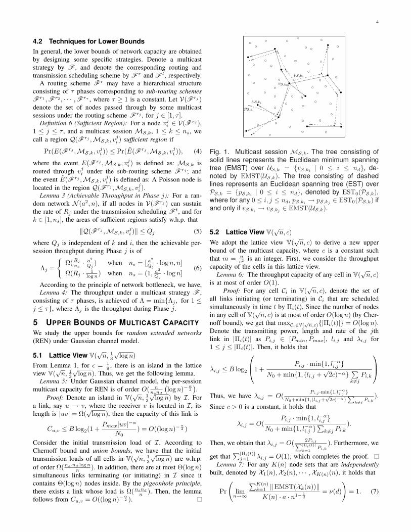
Fig. 1. Multicast session MS,k. The tree consisting ofsolid lines represents the Euclidean minimum spanningtree (EMST) over US,k = vS,ki | 0 ≤ i ≤ nd, de-noted by EMST(US,k). The tree consisting of dashedlines represents an Euclidean spanning tree (EST) overPS,k = pS,ki

| 0 ≤ i ≤ nd, denoted by EST0(PS,k),where for any 0 ≤ i, j ≤ nd, pS,ki → pS,kj ∈ EST0(PS,k) ifand only if vS,ki → vS,kj ∈ EMST(US,k).

5.2 Lattice View V(√

n, c)We adopt the lattice view V(

√n, c) to derive a new upper

bound of the multicast capacity, where c is a constant suchthat m = n

c2 is an integer. First, we consider the throughputcapacity of the cells in this lattice view.

Lemma 6: The throughput capacity of any cell in V(√

n, c)is at most of order O(1).

Proof: For any cell Ci in V(√

n, c), denote the set ofall links initiating (or terminating) in Ci that are scheduledsimultaneously in time t by Πi(t). Since the number of nodesin any cell of V(

√n, c) is at most of order O(log n) (by Cher-

noff bound), we get that maxCi∈V(√

n,c)|Πi(t)| = O(log n).Denote the transmitting power, length and rate of the jthlink in |Πi(t)| as Pi,j ∈ [Pmin, Pmax], li,j and λi,j for1 ≤ j ≤ |Πi(t)|. Then, it holds that

λi,j ≤ B log2

1 +

Pi,j ·min1, l−αi,j

N0 + min1, (li,j +√

2c)−α ∑k 6=j

Pi,k

Thus, we have λi,j = O(Pi,j ·min1,l−α

i,j

N0+min1,(li,j+√

2c)−α∑

k 6=jPi,k

).

Since c > 0 is a constant, it holds that

λi,j = O(Pi,j ·min1, l−α

i,j N0 + min1, l−α

i,j ∑

k 6=j Pi,k

).

Then, we obtain that λi,j = O( 2Pi,j∑|Πi(t)|k=1

Pi,k

). Furthermore, we

get that∑|Πi(t)|

j=1 λi,j = O(1), which completes the proof.Lemma 7: For any K(n) node sets that are independently

built, denoted by X1(n),X2(n), · · · ,XK(n)(n), it holds that

Pr

(lim

n→∞

∑K(n)k=1 ‖EMST(Xk(n))‖

K(n) · a · n1− 1d

= ν(d)

)= 1. (7)

5

Lemma 8: For all multicast sessions MS,k (1 ≤ k ≤ ns),it holds that when nd = o( n

log n ),∑ns

k=1‖EMST(MS,k)‖ = Ω(ns ·

√nd · n).

Proof: Recall that for any multicast session, say MS,k,a set of nd + 1 points are chosen randomly and inde-pendently from the deployment region A(n), denoted byPS,k = pS,k0 , pS,k1 , · · · , pS,knd

. Let EMST(PS,k) denotethe Euclidean minimum spanning tree (EMST) based on theset PS,k. Then, by Lemma 7, it holds almost surely that

∑ns

k=1‖EMST(PS,k)‖ = Θ(ns

√ndn). (8)

Next, we build an Euclidean spanning tree (EST) T0 =EST0(PS,k) on the basis of EMST(US,k), as illustrated inFig.1. Then, ‖EST0(PS,k‖ ≥ ‖EMST(PS,k‖. Denote anyedge pS,ki

→ pS,kjby < i, j > without confusion, then

‖EMST(US,k)‖≥ ∑

<i,j>∈T0

(|pS,kipS,kj | − |pS,kivS,ki | − |pS,kj vS,kj |)= ‖EST0(PS,k‖ −

∑<i,j>∈T0

(|pS,kivS,ki |+ |pS,kj vS,kj |)≥ ‖EMST(PS,k‖ − 2nd ·max|pS,kivS,ki |, for 0 ≤ i ≤ nd.

Let D(pS,ki , r(n)) denote the disk centered at the pointpS,ki with a radius r(n). Then, the number of nodes inD(pS,ki , r(n)), denoted by N(pS,ki , r(n)), follows a Poissondistribution of mean π · (r(n))2. Let r(n) = 3

√log n, accord-

ing to Chernoff bound, we have

Pr(

N(pS,ki , 3√

log n) ≤ 9π

2· log n

)≤ 1

n3.

Define Nmin := minN(pS,ki , r(n)), for all 0 ≤ i ≤ nd, 1 ≤k ≤ ns. By union bounds, we get

Pr(

Nmin ≤ 9π

2· log n

)≤ ns · (nd + 1) · 1

n3≤ 1

n→ 0,

which implies that for any 1 ≤ k ≤ ns and 0 ≤ i ≤ nd,|pS,kivS,ki | ≤ r(n) = 3

√log n, w.h.p.. Hence,

ns∑

k=1

‖EMST(US,k)‖ ≥ns∑

k=1

‖EMST(PS,k‖−6ns ·nd ·√

log n.

Following nd = o( nlog n ) and Equation (8), it holds that∑ns

k=1 ‖EMST(PS,k‖ = ω(6ns · nd ·√

log n). Thus,∑ns

k=1‖EMST(US,k)‖ = Ω(

∑ns

k=1‖EMST(PS,k‖).

Combining with Equation (8), we complete the proof.Lemma 9: The per-session multicast capacity for REN is

of order O(√

nns√

nd) when nd = o( n

log n ).Proof: For each multicast tree TS,k, denote the number

of cells in V(√

n, c) used by it as N(TS,k,√

n, c). Accordingto Lemma 2, it holds that

∑ns

k=1N(TS,k,

√n, c) = Ω

(∑ns

k=1‖EMST(MS,k)‖

)

(9)Case 1: When nd : (1, n/log n).Combining Lemma 8 with Equation (9), we obtain that∑ns

k=1 N(TS,k,√

n, c) = Ω(ns√

ndn) when nd = o( nlog n ).

By pigeonhole principle, there is at least one cell that willbe used by at least Ω(ns

√nd√n

) sessions. By Lemma 6, the totalthroughput capacity of any cell in V(

√n, c) is of order O(1).

Thus, under any strategy, due to the congestion in some cells,the multicast throughput is at most of order O(

√n

ns√

nd).

Case 2: When nd = Θ(1).The problem degenerates into the case of unicast sessions.

From the result in [21], the per-session unicast capacity forREN is of order O(

√n

ns), i.e., O(

√n

ns√

nd) for nd = Θ(1).

Combining two cases, we complete the proof.Based on Lemma 5 and Lemma 9, we obtain Theorem 4

by performing some simple algebraic manipulations.Theorem 4: The per-session multicast capacity for random

extended networks is of orderO(

√n

ns√

nd) when nd : [1, n

(log n)α ]O( n

nsnd· (log n)−

α2 ) when nd : [ n

(log n)α , n]

By letting ns = Θ(n), we get Theorem 1.

6 LOWER BOUNDS OF MULTICAST CAPACITY

We derive the lower bounds on multicast capacity for RENby proposing two multicast strategies, denoted by F andS , respectively. Our multicast strategies are cell-based, thenwe first recall a new notion called scheme lattice [28] forsuccinctness of the description.

Definition 7 (Scheme Lattice): Divide a square deploymentregion A(a2) = [0, a]2 into a lattice consisting of square cellsof side length g, we call the lattice scheme lattice and denote itby L(a, g, θ), where θ ∈ [0, π

4 ] is the minimum angle betweenthe sides of the deployment region and produced cells.

6.1 Highways SystemThe highway system consists of highways of two levels. Thefirst are the first-class highways (FHs), indeed the highwaysin [20]. The second are the second-class highways (SHs) thatare built without using percolation theory.

6.1.1 First-Class Highways (FHs)We recall the construction of FHs based on percolation theory[20], and introduce the transmission scheduling by which eachFH can sustain a rate of constant order.

Construction of FHs: The FHs are built based on thescheme lattice L(

√n, c, π

4 ), as depicted in Fig.2(a). Then,there are m2 cells in L(

√n, c, π

4 ), where m =⌈√

n/√

2c⌉

(we can adjust the value of c such that√

n/√

2c is an integer).Let N(Ci) denote the number of Poisson points inside cell Ci,which is a Poisson random variable with mean c2. For all i,the probability that a square Ci contains at least one Poissonpoint (N(Ci) ≥ 1) is p ≡ 1− e−c2

. We say a square is openif it contains at least one point, and closed otherwise. Thenany square is open with probability p, independently from eachother. Based on L(

√n, c, π

4 ), we draw a horizontal edge acrosshalf of the squares, and a vertical edge across the others, toobtain a scheme lattice L(

√n,√

2c, 0), as shown in Fig.2(a).We say a given edge ~ in L(

√n,√

2c, 0) is open if the cell inL(√

n, c, π4 ), crossed by ~, is open, and call a path comprised

6

θ1 log n

(a) First-class highways (b) Second-class highways

Fig. 2. (a) The bold polygonal line represents an openpath consisting of open edges. A vertical first-class high-way (FH) is illustrated by a polygonal line whose inflexionsare called first-class stations. (b) The bold lines connect-ing the nodes, called second-class stations, represent thesecond-class highways (SHs).

of edges in L(√

n,√

2c, 0) open if it contains only open edges.Based on an open path connecting the left side of A(n) withits right side (or connecting the upper side of A(n) with itsbottom side), as illustrated in Fig.2(a), choose a node fromeach cell in L(

√n, c, π

4 ) corresponding to the open edges ofthe open path, and connect a pair of nodes from two adjacentcells, we finally obtain a crossing path. We call those crossingpaths first-class highways (FHs).

Density of FHs: For a given κ > 0, partition the schemelattice L(

√n, c, π

4 ) into horizontal (or vertical) rectangle slabsof size m× (κ log m− εm) (or (κ log m− εm)×m), denotedby Rh

i (or Rvi ). Denote the number of disjoint horizontal (or

vertical) FHs within Rhi (or Rv

i ) by Nhi (or Nv

i ). It holds thatLemma 10: ( [20]) For every κ and p ∈ (5/6, 1) satisfying

2 + κ log(6(1− p)) < 0, there exists a δ = δ(κ, p) such that

limm→∞

Pr(Nh ≥ δ log m) = 1, limm→∞

Pr(Nv ≥ δ log m) = 1,

where Nh = mini Nhi and Nv = mini Nv

i .Notations for FHs: To simplify the description, we assume

that there are exactly δ log m horizontal (or vertical) FHs ineach horizontal (or vertical) slab, which does not change theresults in order sense. According to lemma 10, we can furtherdivide every slab into δ log m slices of size l × √

n, wherel = (κ log m−εm)

δ log m . Hence, we can define the mapping amongthe slabs, slices, and FHs. Please see the details in Table 1.The following are some remarks.

1) Any slice can and only can project to an FH containedby the slab that posses the slice, which ensures that thedistance from any points in the slice to the correspondinghighway is at most of κ log m− εm.

2) For a node v and horizontal slice Shi ∈ Sh (or vertical

slice Svi ∈ Sv), if v is located in Sh

i (or Svi ), then fh(v) =

gh(Shi ) (or fv(v) = gv(Sv

i )).3) ψh(hh

k) (or ψv(hvk)) denotes the horizontal (or vertical)

slab completely containing the horizontal (or vertical) FHhk (or hv

k).Transmission Scheduling for FHs: To schedule the FHs,

we use a 9-TDMA scheduling scheme based on the scheme

TABLE 1Notations for FHs

Notation Meaning

Rhi i-th horizontal slab of size m× (κ log m− εm)

Rvi i-th vertical slab of size (κ log m− εm)×m

Rh (or Rv) the set of all horizontal (or vertical) slabs

Shj j-th horizontal slice of size m× κ log m−εm

δ log m

Svj j-th vertical slice of size κ log m−εm

δ log m×m

Sh (or Sv) the set of all horizontal (or vertical) slices

hhk (or hv

k) k-th horizontal (or vertical) FH

Hh (or Hv) the set of all horizontal (or vertical) FHs

gh:Sh → Hh a bijection from horizontal slices to horizontal FHs

gv :Sv → Hv a bijection from vertical slices to vertical FHs

fh : V → Hh a function from nodes to horizontal FHs

fv : V → Hv a function from nodes to vertical FHs

ψh : Hh → Rh a function from horizontal FHs to horizontal slabs.

ψv : Hv → Rv a function from vertical FHs to vertical slabs.

lattice L(√

n, c, π4 ) by letting K = 3 and d = 1 in Fig. 4

of [20]. According to Theorem 3 in [20], all FHs can sustainw.h.p. the rate of order Ω(1).

6.1.2 Second-Class Highways (SHs)We build the SHs and design the transmission scheduling toachieve the rate of order Ω((log n)−

α2 ) along each SH.

Construction of SHs: The SHs are constructed based on thescheme lattice L(

√n, σ

√log n−εn, 0), as depicted in Fig.2(b),

where σ > 0 is a constant and we choose εn > 0 as thesmallest value such that

√n/(σ

√log n− εn) is an integer. It

is obvious that εn = o(1). Then there are n/(σ√

log n− εn)2

cells. Let N(Cj) be the number of Poisson nodes insidea cell Cj , which is a Poisson random variable with mean(σ√

log n − εn)2. Furthermore, we define the uniform lowerbound of N(Cj) as NC .

To ensure the feasibility of the method to construct SHs,we give the following lemma.

Lemma 11: For any %, % > 1 + log %, and σ, σ2 ≥4%

(2%−log %−1) , each cell in L(√

n, σ√

log n − εn, 0) containsw.h.p. no less than θ1 log n nodes, where θ1 is a constant withθ1 = σ2

2% .Proof: Since (σ

√log n − εn)2 > 1

2σ2 log n, as n → ∞,according to Chernoff bound and union bounds, we have

Pr(NC ≤ σ2·log n

2%

)≤ 2n

σ2·log nPr(N(Cj) ≤ σ2·log n

2%

)

≤ 2nσ2·log n

nσ22%

nσ22· nσ2·log %

2% = 2

σ2·log n·nσ22 −1− (1+log %)σ2

2%

Thus, when we choose % with % > 1 + log % and σ withσ2 ≥ 2%

ρ−(1+log ρ) , it holds that Pr(NC ≤ σ2·log n2% ) → 0.

We call each row (or column) of L(√

n, σ√

log n − εn, 0)row-slab (or column-slab), denoted by Rh

i (or Rvi ). In each

7

concurrent θ1 log n links

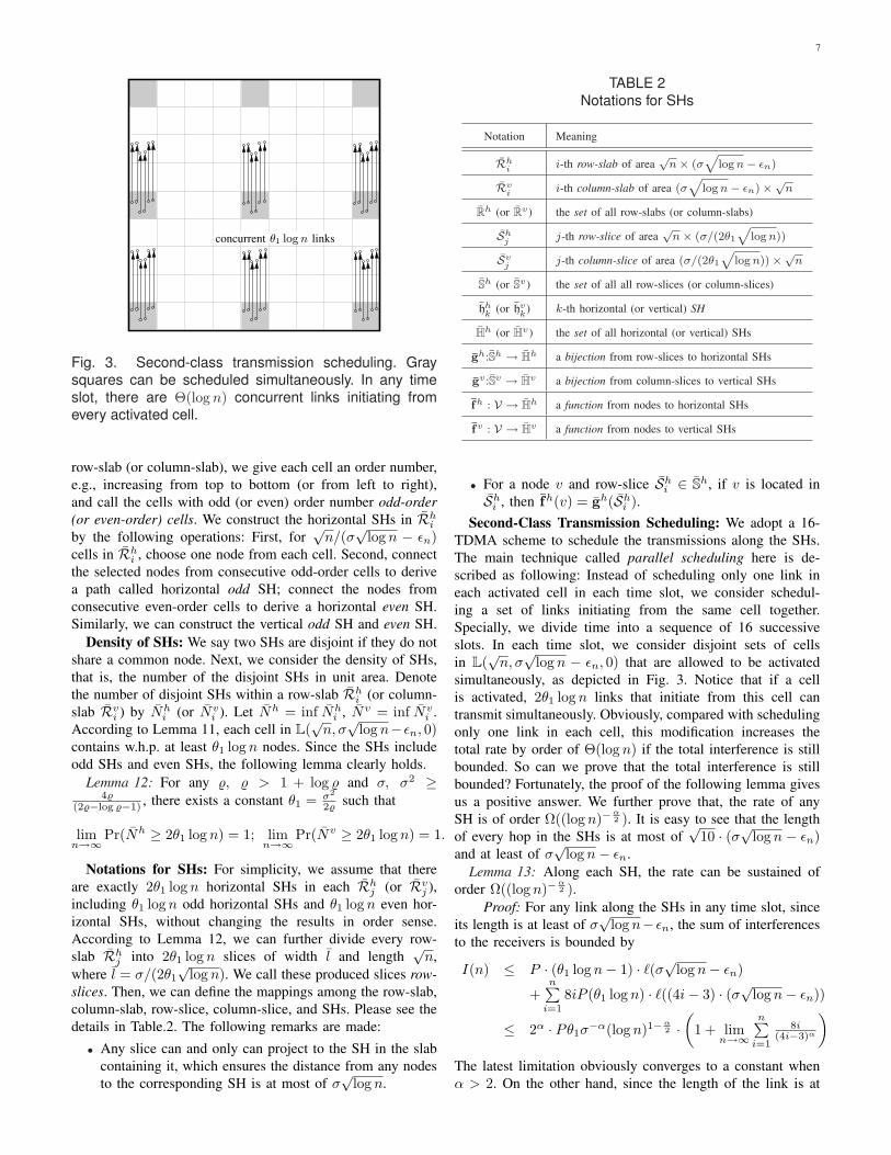
Fig. 3. Second-class transmission scheduling. Graysquares can be scheduled simultaneously. In any timeslot, there are Θ(log n) concurrent links initiating fromevery activated cell.

row-slab (or column-slab), we give each cell an order number,e.g., increasing from top to bottom (or from left to right),and call the cells with odd (or even) order number odd-order(or even-order) cells. We construct the horizontal SHs in Rh

i

by the following operations: First, for√

n/(σ√

log n − εn)cells in Rh

i , choose one node from each cell. Second, connectthe selected nodes from consecutive odd-order cells to derivea path called horizontal odd SH; connect the nodes fromconsecutive even-order cells to derive a horizontal even SH.Similarly, we can construct the vertical odd SH and even SH.

Density of SHs: We say two SHs are disjoint if they do notshare a common node. Next, we consider the density of SHs,that is, the number of the disjoint SHs in unit area. Denotethe number of disjoint SHs within a row-slab Rh

i (or column-slab Rv

i ) by Nhi (or Nv

i ). Let Nh = inf Nhi , Nv = inf Nv

i .According to Lemma 11, each cell in L(

√n, σ

√log n− εn, 0)

contains w.h.p. at least θ1 log n nodes. Since the SHs includeodd SHs and even SHs, the following lemma clearly holds.

Lemma 12: For any %, % > 1 + log % and σ, σ2 ≥4%

(2%−log %−1) , there exists a constant θ1 = σ2

2% such that

limn→∞

Pr(Nh ≥ 2θ1 log n) = 1; limn→∞

Pr(Nv ≥ 2θ1 log n) = 1.

Notations for SHs: For simplicity, we assume that thereare exactly 2θ1 log n horizontal SHs in each Rh

j (or Rvj ),

including θ1 log n odd horizontal SHs and θ1 log n even hor-izontal SHs, without changing the results in order sense.According to Lemma 12, we can further divide every row-slab Rh

j into 2θ1 log n slices of width l and length√

n,where l = σ/(2θ1

√log n). We call these produced slices row-

slices. Then, we can define the mappings among the row-slab,column-slab, row-slice, column-slice, and SHs. Please see thedetails in Table.2. The following remarks are made:

• Any slice can and only can project to the SH in the slabcontaining it, which ensures the distance from any nodesto the corresponding SH is at most of σ

√log n.

TABLE 2Notations for SHs

Notation Meaning

Rhi i-th row-slab of area

√n× (σ

√log n− εn)

Rvi i-th column-slab of area (σ

√log n− εn)×√n

Rh (or Rv) the set of all row-slabs (or column-slabs)

Shj j-th row-slice of area

√n× (σ/(2θ1

√log n))

Svj j-th column-slice of area (σ/(2θ1

√log n))×√n

Sh (or Sv) the set of all all row-slices (or column-slices)

hhk (or hv

k) k-th horizontal (or vertical) SH

Hh (or Hv) the set of all horizontal (or vertical) SHs

gh:Sh → Hh a bijection from row-slices to horizontal SHs

gv :Sv → Hv a bijection from column-slices to vertical SHs

fh : V → Hh a function from nodes to horizontal SHs

fv : V → Hv a function from nodes to vertical SHs

• For a node v and row-slice Shi ∈ Sh, if v is located in

Shi , then fh(v) = gh(Sh

i ).Second-Class Transmission Scheduling: We adopt a 16-

TDMA scheme to schedule the transmissions along the SHs.The main technique called parallel scheduling here is de-scribed as following: Instead of scheduling only one link ineach activated cell in each time slot, we consider schedul-ing a set of links initiating from the same cell together.Specially, we divide time into a sequence of 16 successiveslots. In each time slot, we consider disjoint sets of cellsin L(

√n, σ

√log n − εn, 0) that are allowed to be activated

simultaneously, as depicted in Fig. 3. Notice that if a cellis activated, 2θ1 log n links that initiate from this cell cantransmit simultaneously. Obviously, compared with schedulingonly one link in each cell, this modification increases thetotal rate by order of Θ(log n) if the total interference is stillbounded. So can we prove that the total interference is stillbounded? Fortunately, the proof of the following lemma givesus a positive answer. We further prove that, the rate of anySH is of order Ω((log n)−

α2 ). It is easy to see that the length

of every hop in the SHs is at most of√

10 · (σ√log n − εn)and at least of σ

√log n− εn.

Lemma 13: Along each SH, the rate can be sustained oforder Ω((log n)−

α2 ).

Proof: For any link along the SHs in any time slot, sinceits length is at least of σ

√log n− εn, the sum of interferences

to the receivers is bounded by

I(n) ≤ P · (θ1 log n− 1) · `(σ√log n− εn)

+n∑

i=1

8iP (θ1 log n) · `((4i− 3) · (σ√log n− εn))

≤ 2α · Pθ1σ−α(log n)1−

α2 ·

(1 + lim

n→∞

n∑i=1

8i(4i−3)α

)

The latest limitation obviously converges to a constant whenα > 2. On the other hand, since the length of the link is at

8

column−slab

column−slice

6

5

4

32

1

7

uij

whj

wvi

whi

uvij

uhij

wvj

vj

vi

κ log m− εm

σ

√log n− εn

fh(vi)

fv(vj)

fh(vj)

fv(vi)

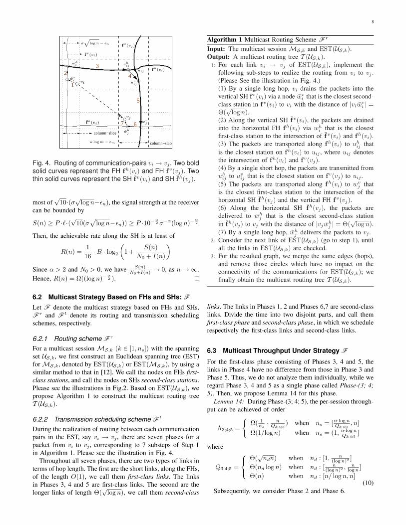
Fig. 4. Routing of communication-pairs vi → vj . Two boldsolid curves represent the FH fh(vi) and FH fv(vj). Twothin solid curves represent the SH fv(vi) and SH fh(vj).

most of√

10·(σ√log n−εn), the signal strength at the receivercan be bounded by

S(n) ≥ P ·`·(√

10(σ√

log n−εn)) ≥ P ·10−α2 σ−α(log n)−

α2

Then, the achievable rate along the SH is at least of

R(n) =116·B · log2

(1 +

S(n)N0 + I(n)

)

Since α > 2 and N0 > 0, we have S(n)N0+I(n) → 0, as n →∞.

Hence, R(n) = Ω((log n)−α2 ).

6.2 Multicast Strategy Based on FHs and SHs: F

Let F denote the multicast strategy based on FHs and SHs,F r and F t denote its routing and transmission schedulingschemes, respectively.

6.2.1 Routing scheme F r

For a multicast session MS,k (k ∈ [1, ns]) with the spanningset US,k, we first construct an Euclidean spanning tree (EST)for MS,k, denoted by EST(US,k) or EST(MS,k), by using asimilar method to that in [12]. We call the nodes on FHs first-class stations, and call the nodes on SHs second-class stations.Please see the illustrations in Fig.2. Based on EST(US,k), wepropose Algorithm 1 to construct the multicast routing treeT (US,k).

6.2.2 Transmission scheduling scheme F t

During the realization of routing between each communicationpairs in the EST, say vi → vj , there are seven phases for apacket from vi to vj , corresponding to 7 substeps of Step 1in Algorithm 1. Please see the illustration in Fig. 4.

Throughout all seven phases, there are two types of links interms of hop length. The first are the short links, along the FHs,of the length O(1), we call them first-class links. The linksin Phases 3, 4 and 5 are first-class links. The second are thelonger links of length Θ(

√log n), we call them second-class

Algorithm 1 Multicast Routing Scheme F r

Input: The multicast session MS,k and EST(US,k).Output: A multicast routing tree T (US,k).

1: For each link vi → vj of EST(US,k), implement thefollowing sub-steps to realize the routing from vi to vj .(Please See the illustration in Fig. 4.)(1) By a single long hop, vi drains the packets into thevertical SH fv(vi) via a node wv

i that is the closest second-class station in fv(vi) to vi with the distance of |viw

vi | =

Θ(√

log n).(2) Along the vertical SH fv(vi), the packets are drainedinto the horizontal FH fh(vi) via wh

i that is the closestfirst-class station to the intersection of fv(vi) and fh(vi).(3) The packets are transported along fh(vi) to uh

ij thatis the closest station on fh(vi) to uij , where uij denotesthe intersection of fh(vi) and fv(vj).(4) By a single short hop, the packets are transmitted fromuh

ij to uvij that is the closest station on fv(vj) to uij .

(5) The packets are transported along fh(vi) to wvj that

is the closest first-class station to the intersection of thehorizontal SH fh(vj) and the vertical FH fv(vj).(6) Along the horizontal SH fh(vj), the packets aredelivered to wh

j that is the closest second-class stationin fh(vj) to vj with the distance of |vjw

hj | = Θ(

√log n).

(7) By a single long hop, whj delivers the packets to vj .

2: Consider the next link of EST(US,k) (go to step 1), untilall the links in EST(US,k) are checked.

3: For the resulted graph, we merge the same edges (hops),and remove those circles which have no impact on theconnectivity of the communications for EST(US,k); wefinally obtain the multicast routing tree T (US,k).

links. The links in Phases 1, 2 and Phases 6,7 are second-classlinks. Divide the time into two disjoint parts, and call themfirst-class phase and second-class phase, in which we schedulerespectively the first-class links and second-class links.

6.3 Multicast Throughput Under Strategy F

For the first-class phase consisting of Phases 3, 4 and 5, thelinks in Phase 4 have no difference from those in Phase 3 andPhase 5. Thus, we do not analyze them individually, while weregard Phase 3, 4 and 5 as a single phase called Phase-(3; 4;5). Then, we propose Lemma 14 for this phase.

Lemma 14: During Phase-(3; 4; 5), the per-session through-put can be achieved of order

Λ3;4;5 =

Ω( 1

ns· n

Q3;4;5) when ns = [n·log n

Q3;4;5, n]

Ω(1/log n) when ns = (1, n·log nQ3;4;5

]

where

Q3;4;5 =

Θ(√

ndn) when nd : [1, n(log n)2 ]

Θ(nd log n) when nd : [ n(log n)2 , n

log n ]Θ(n) when nd : [n/ log n, n]

(10)Subsequently, we consider Phase 2 and Phase 6.

9

Lemma 15: In Phase 2, the per-session throughput can beachieved of order

Λ2 =

Ω(R2

ns· n

Q2) when ns = [ n

Q2· log n, n]

Ω(R2/log n) when ns = (1, nQ2· log n]

(11)

where R2 = Ω((log n)−α2 ), Q2 = minordernd

√log n, n.

By a similar procedure to the proof of Lemma 15, we canget the following result for Phase 6.

Lemma 16: In Phase 6, the per-session multicast throughputcan be achieved of the same order as in Phase 2.

During Phases 1 and 7, like Phases 2 and 6, we also use a16-TDMA scheme to schedule the links of length Θ(

√log n)

in parallel, by which we can ensure that every link achievesthe rate of order Ω((log n)−

α2 ). On the other hand, there is no

relay burden on the nodes in Phases 1 and 7 due to the single-hop pattern, thus, it is easy to obtain the following result.

Lemma 17: minorderΛ1,Λ7 = Ω(maxorderΛ2, Λ6).Combining Lemmas 14, 15, 16 and 17, we obtain the

following result according to Lemma 4.Theorem 5: By using the multicast strategy F , the per-

session multicast throughput is achieved of order:When nd = O(n/

√log n),

Ω( 1

(log n)1+α2

) when ns : (1, n log nΓ ]

Ω(minorder

nnsΓ , 1

(log n)1+α2) when ns : [n log n

Γ ,n√

log n

nd]

Ω(minorder

nnsΓ , n

nsnd(log n)α+1

2) when ns : [n

√log n

nd, n]

When nd = Ω(n/√

log n),

Ω( n

nsnd(log n)α+1

2) when ns : (1, n

√log n/nd]

Ω( 1

(log n)1+α2

) when ns : [n√

log n/nd, n]

where Γ := Q3;4;5 is defined in Equation (10).

6.4 Multicast Strategy Based on Only SHs: S

Now, we devise another multicast strategy, denoted by S ,which is only based on the SHs. The routing scheme is denotedby S r, and is described in Algorithm 2. For the transmissionscheduling, denoted by S t, we only need to implement thesecond-class transmission scheduling since no other types oflinks exist. It can be shown that if the bottleneck of F r liesin its second-class phase, the multicast throughput under Sis not less than that under F . Specifically, we have

Theorem 6: By using the multicast strategy S , the per-session multicast throughput is achieved of order

Ω( n

(log n)α2 ns·Q

) when ns = Ω(n·log nQ

)

Ω(1/(log n)1+α2 ) when ns = O(n·log n

Q)

where Q =

Θ(

√ndnlog n ) when nd = O( n

log n )

Θ(nd) when nd = Ω( nlog n ).

Proof: The throughputs during Phase 1 and Phase 5 arenot less than those during other phases, implying that thebottleneck of the entire routing lies on SHs. According toLemma 13, the rate of each SH can be achieved of orderΩ((log n)−

α2 ). On the other hand, by using a similar procedure

Algorithm 2 Multicast Routing Scheme S r

Input: The multicast session MS,k and EST(US,k).Output: A multicast routing tree T (US,k).

1: For each link vi → vj of EST(US,k), implement thefollowing sub-steps to realize the routing vi → vj .(1) By a single hop, vi drains the packets into the verticalSH fv(vi) via wv

i that is the closest second-class stationto vi on fv(vi) with the distance of |viw

vi | = Θ(

√log n)).

(2) The packets are transported along fv(vi) to uvij that

is the closest second-class station on fv(vi) to uij , whereuij denotes the intersection of fv(vi) and fh(vj);(3) By a single hop, the packets are transmitted from uv

ij

to uhij that is the closest station on fh(vj) to uij .

(4) The packets are transported along horizontal SH fh(vj)to wh

j that is the closest second-class station to vj onfh(vj) with the distance of |vjw

hj | = Θ(

√log n).

(5) By a single hop, whj delivers the packets to vj .

2: Consider the next link of EST(US,k) (go to step 1), untilall the links in EST(US,k) are checked.

3: Use the same method as step 3 of F r to obtain the finalmulticast routing tree T (US,k).

to the proof of Lemma 14, we can obtain that the burden ofthe second-class stations is w.h.p. at most of order

O(nsQ/n) when nsQ/n = Ω(log n)O(log n) when nsQ/n = O(log n) (12)

with Q = minorder√nnd/√

log n + nd, n. Hence, wecomplete the proof.

6.5 General Result for Random Extended NetworksCombining Theorem 5 and Theorem 6, we obtain the generalresult in Theorem 7.

Theorem 7: The per-session multicast throughput for ran-dom extended networks can be achieved of order Ω(λ(n)) asdescribed in Table 3.

Theorem 2 can be obtained based on Theorem 7 by lettingns = Θ(n).

As in [12], we design multicast routing schemes basedon the construction of Euclidean spanning trees. Note thatthis way of constructing the spanning tree is not symmetric,which leads that most paths will go through the center area ofthe network. Under such routing, some parts of the networkwill be under a relatively large load, therefore, those partswould become a bottleneck for the multicast sessions, calledlocal bottleneck. In fact, in the derivation of Theorem 2, it isjust this local bottleneck that limits the network throughputunder our schemes, since we take the maximum load of anypart of the network into account. Then, the existence of thelocal bottleneck makes our schemes look non-optimal. While,combining with the upper bounds in Theorem 1, we obtainthat our scheme is optimal (in order sense) in the regimesof nd : [1, n

(log n)α+1 ] and nd : [ nlog n , n]. That implies that

in these regimes of nd, the load at the local bottleneck isat most a constant times of that at other parts of the network.Furthermore, the local bottleneck issue should be fully studied

10

in the future work. Designing a multicast scheme without thelocal bottleneck is a possible solution to close the remaininggap between the upper and lower bounds.

7 LITERATURE REVIEWS

In this section, we mainly review the networking-theoretic ca-pacity scaling laws for random ad hoc network. We summarizethe classifications of this issue in Table 4, and indicate thescope of a related work by a 3-dimensional coordinate (x, y, z)based on Table 4, where x ∈U, B, M, y ∈D, E and z ∈O,Y, G. For instance, (U,E,G) denotes the per-session unicastcapacity for random extended networks (REN) under Gaussianchannel model (GCM).

In REN, there must be some links of length ω(1) underany routing scheme in order to ensure the connectivity ofnetwork. For those links, when the ProM or PhyM is adopted,the rate will be set as a constant order if they can be scheduled,which is over-optimistic and unrealistic for power-constrainedwireless networks. This can explain why we hardly introducethe works on (x,E,z), x ∈U, B, M and z ∈O, Y.Moreover, for RDN, the throughput under the GCM can beequivalently achieved under the ProM and PhyM, if multiplecommunication and interference radii (or the thresholds ofSINR) are permitted under the ProM (or the PhyM). In thefollowing review, we use session patterns as the main index.

Unicast Sessions: In the pioneering work of capacityscaling laws, Gupta and Kumar [2] showed that the orderof (U,D,O) is Θ(1/

√n log n); and they derived the lower

bound and upper bound of (U,D,Y) as Ω(1/√

n log n) andO(1/

√n), respectively, leaving a gap between the upper and

lower bounds of unicast capacity for RDN under PhyM.Franceschetti et al. [20] proposed the hierarchical schemes

based on bond percolation model, under which the lowerbounds of (U,D,G) and (U,E,G) can be both achieved of orderΩ(1/

√n); later, Keshavarz-Haddad et al. [29] derived the

upper bound of (U,D,G) as O(1/√

n), Li et al. [21] proved thatthe upper bound of (U,E,G) is also of O(1/

√n). Combining

the works in [20], [21], [29], one can get that the unicastcapacities for both RDN and REN under Gaussian channelmodel (GCM) are of order Θ(1/

√n).

Broadcast Sessions: According to [13], [30] done byKeshavarz-Haddad et al., and Tavli, respectively, the orderof (B,D,O) is of Θ( 1

n ). Keshavarz-Haddad and Riedi [31]analyzed the essential impact of topology and interference onthe broadcast capacity under the PhyM and GCM. As a part ofthe contributions of [31], the (B,D,Y) and (B,D,G) are provedto be both of order Θ( 1

n ) when the the bandwidth is of aconstant order. For (B,E,G), Zheng [3] proved that the orderis of Θ( (log n)−

α2

n ).Multicast Sessions: Earlier, Jacquet and Rodolakis

[32] showed that the upper bound of (M,D,O) is ofO(1/

√ndn log n). Shakkottai et al. [14] designed a novel

multicast scheme called comb, by which the lower bound of(M,D,O) can be achieved of order Ω(1/

√ndn log n) when

the number of multicast sources, denoted by ns, is nε forsome ε > 0, and the number of destinations per multicastsession, denoted by nd, is n1−ε. Li [12] proved that the order

TABLE 3Achievable Per-Session Multicast Throughput for REN

Range of nd Better Strategy and Order of λ(n)

[1, n(log n)1+α ] F :

(log n)−1−α2 if ns : (1,

√n√

nd· (log n)1+

α2 ]

√n

ns√

ndif ns : [

√n√

nd· (log n)1+

α2 , n]

[ n(log n)1+α , n

(log n)2] F :

(log n)−1−α2 if ns : (1,

n·√

log n

nd]

n

nsnd(log n)α+1

2if ns : [

n·√

log n

nd, n]

[ n(log n)2

, nlog n

] S :

(log n)−1−α2 if ns : (1,

√n·(log n)

32√

nd]

√n

ns√

nd·(log n)α−1

2if ns : [

√n·(log n)

32√

nd, n]

[ nlog n

, n] S :

(log n)−1−α2 if ns : (1, n log n

nd]

n

ns·nd·(log n)α2

if ns : [n log nnd

, n]

of (M,D,O) is of Θ(1/√

ndn log n) when nd = O(n/log n),and is of Θ(1/n) when nd = Ω(n/log n). By using anovel technique called arena, Keshavarz-Haddad and Riedi[19] proved all the upper bounds of (M,D,O), (M,D,Y) and(M,D,G) are of order O( 1√

nnd) when nd : [1, n

(log n)2 ], are ofO( 1

nd log n ) when nd : [ n(log n)2 , n

log n ], and are of O(1) whennd : [ n

log n , n]. Furthermore, they derived the lower boundsof (M,D,Y) and (M,D,G) are of order Ω( 1√

nnd) when nd :

[1, n(log n)3 ], are of Ω( (log n)−3/2

nd) when nd : [ n

(log n)3 , n(log n)2 ],

are of Ω( 1√nnd log n

) when nd : [ n(log n)2 , n

log n ], and are of

Ω(1) when nd : [ nlog n , n].

For (M,E,G), Li et al. [21] proposed a lower bound asΩ(

√n

ns√

nd) when nd = O( n

(log n)2α+6 ) and ns = Ω(n12+θ),

where θ > 0 is any positive constant. Note that we focus on(M,E,G) in this paper. We derive the more tight lower boundsof (M,E,G) for all cases of ns : (1, n] by introducing the two-level highway system and parallel transmission scheduling,and propose the upper bounds based on some new arguments.

There are some other types of sessions, such as gathercast(many-to-one sessions) [33], [34], anycast [35] and manycast[36], etc. We omit the review of works for those sessions,since they are not directly relevant to the scope of this paper.

8 CONCLUSION

We study the networking-theoretic multicast capacity boundsfor random extended networks (REN) under Gaussian Channelmodel. Based on percolation theory, we propose two mul-ticast strategies for REN and derive the achievable multi-cast throughput by considering all cases of ns : (1, n] andnd : [1, n]. We show that under the assumption of ns = Θ(n),the per-session multicast throughput derived by our scheme isorder-optimal when nd = O( n

(log n)α+1 ) or nd = Ω( nlog n ).

There are still gaps between the lower bounds and upperbounds on multicast capacity of REN for some regimes ofnd, i.e., nd : [ n

(log n)α+1 , nlog n ]. An interesting and challenging

11

TABLE 4Networking-Theoretic Capacity Scaling Laws for Random Ad Hoc Networks

Capacity of Session Patterns Scaling Models (Density) Communication Models

1 U: Unicast Capacity D: Random Dense Networks (RDN) O: Protocol Model (ProM)

2 B: Broadcast Capacity E: Random Extended Networks (REN) Y: Physical Model (PhyM)

3 M: Multicast Capacity G: Gaussian Channel Model (GCM)

issue is to close the gaps on multicast capacity by presentingpossibly new tighter upper bounds, and lower bounds, anddesigning corresponding algorithms to achieve the asymptoticmulticast capacity.

ACKNOWLEDGMENTS

The authors would like to thank the anonymous reviewersfor their constructive comments. The research of authors ispartially supported by the National Basic Research Programof China (973 Program) under grants No. 2010CB328101 andNo. 2010CB334707, the Program for Changjiang Scholarsand Innovative Research Team in University, the ShanghaiKey Basic Research Project under grant No. 10DJ1400300,the Expo Science and Technology Specific Projects of Chinaunder grant No. 2009BAK43B37, the NSF CNS-0832120 andCNS-1035894, the National Natural Science Foundation ofChina under grant No. 60828003, the Program for ZhejiangProvincial Key Innovative Research Team, and the Programfor Zhejiang Provincial Overseas High-Level Talents (One-hundred Talents Program).

REFERENCES

[1] C. Wang, X.-Y. Li, C. Jiang, S. Tang, and Y. Liu, “Scaling laws onmulticast capacity of large scale wireless networks,” in Proc. IEEEINFOCOM 2009.

[2] P. Gupta and P. R. Kumar, “The capacity of wireless networks,” IEEETransactions on Information Theory, vol. 46, no. 2, pp. 388–404, 2000.

[3] R. Zheng, “Asymptotic bounds of information dissemination in power-constrained wireless networks,” IEEE Transactions on Wireless Commu-nications, vol. 7, no. 1, pp. 251–259, Jan. 2008.

[4] L. Xie and P. Kumar, “A network information theory for wirelesscommunication: scaling laws and optimal operation,” IEEE Transactionson Information Theory, vol. 50, no. 5, pp. 748–767, 2004.

[5] A. OzgUr, O. LEvEque, and D. Tse, “Hierarchical Cooperation AchievesOptimal Capacity Scaling in Ad Hoc Networks,” IEEE Transactions onInformation Theory, vol. 53, no. 10, pp. 3549–3572, 2007.

[6] S. Yi, Y. Pei, and S. Kalyanaraman, “On the capacity improvement ofad hoc wireless networks using directional antennas,” in Proc. ACMMobiHoc 2003.

[7] S. R. Kulkarni and P. Viswanath, “A deterministic approach to through-put scaling in wireless networks,” IEEE Transactions on InformationTheory, vol. 50, no. 6, pp. 1041–1049, 2004.

[8] B. Liu, Z. Liu, and D. Towsley, “On the capacity of hybrid wirelessnetworks,” in Proc. IEEE INFOCOM 2003.

[9] U. C. Kozat and L. Tassiulas, “Throughput capacity of random ad hocnetworks with infrastructure support,” in Proc. ACM MobiCom 2003.

[10] A. Zemlianov and G. de Veciana, “Capacity of ad hoc wireless net-works with infrastructure support,” IEEE Journal on Selected Areas inCommunications, vol. 23, no. 3, pp. 657–667, 2005.

[11] J. Gomez and A. T. Campbell, “Variable-range transmission powercontrol in wireless ad hoc networks,” IEEE Transactions on MobileComputing, vol. 6, no. 1, pp. 87–99, 2007.

[12] X.-Y. Li, “Multicast capacity of wireless ad hoc networks,” IEEE/ACMTransactions on Networking, vol. 17, no. 3, pp. 950–961, 2009.

[13] A. Keshavarz-Haddad, V. Ribeiro, and R. Riedi, “Broadcast capacity inmultihop wireless networks,” in Proc. ACM MobiCom 2006.

[14] X. Shakkottai, S. Liu, and R. Srikant, “The multicast capacity of largemultihop wireless networks,” in Proc. ACM MobiHoc 2007.

[15] X. Wang, Y. Bei, Q. Peng, and L. Fu, “Speed improves delay-capacitytradeoff in motioncast,” to appear in IEEE Transactions on Parallel andDistributed Systems, 2011.

[16] S. Toumpis and A. J. Goldsmith, “Capacity regions for wireless adhoc networks,” IEEE Transactions on Wireless Communications, vol. 2,no. 4, pp. 736–748, 2003.

[17] T. Cover and J. Thomas, Elements of information theory. Wiley, 2006.[18] A. Agarwal and P. Kumar, “Capacity bounds for ad hoc and hybrid

wireless networks,” ACM SIGCOMM Computer Communication Review,vol. 34, no. 3, pp. 71–81, 2004.

[19] A. Keshavarz-Haddad and R. Riedi, “Multicast capacity of large homo-geneous multihop wireless networks,” in Proc. IEEE WiOpt 2008.

[20] M. Franceschetti, O. Dousse, D. Tse, and P. Thiran, “Closing the gapin the capacity of wireless networks via percolation theory,” IEEETransactions on Information Theory, vol. 53, no. 3, pp. 1009–1018,2007.

[21] X.-Y. Li, Y. Liu, S. Li, and S. Tang, “Multicast capacity of wireless adhoc networks under Gaussian channel model,” IEEE/ACM Transactionson Networking, vol. 18, no. 4, pp. 1145–1157, 2010.

[22] L. Xie and P. Kumar, “On the path-loss attenuation regime for positivecost and linear scaling of transport capacity in wireless networks,”IEEE/ACM Transactions on Networking, vol. 14, pp. 2313–2328, 2006.

[23] O. Dousse, M. Franceschetti, and P. Thiran, “Information theoreticbounds on the throughput scaling of wireless relay networks,” in Proc.IEEE INFOCOM 2005.

[24] A. OzgUr, O. LEvEque, and E. Preissmann, “Scaling Laws for One-andTwo-Dimensional Random Wireless Networks in the Low-AttenuationRegime,” IEEE Transactions on Information Theory, vol. 53, no. 10, pp.3573–3585, 2007.

[25] S. Ahmad, A. Jovicic, and P. Viswanath, “On outer bounds to thecapacity region of wireless networks,” IEEE/ACM Transactions onNetworking, vol. 14, pp. 2770–2776, 2006.

[26] O. Leveque and I. Telatar, “Information-theoretic upper bounds on thecapacity of large extended ad hoc wireless networks,” IEEE Transactionson Information Theory, vol. 51, no. 3, pp. 858–865, 2005.

[27] C. Hu, X. Wang, D. Nie, and J. Zhao, “Multicast scaling laws withhierarchical cooperation,” in Proc. IEEE INFOCOM 2010.

[28] C. Wang, X.-Y. Li, C. Jiang, S. Tang, and Y. Liu, “Multicast throughputfor hybrid wireless networks under Gaussian channel model,” to appearin IEEE Transactions on Mobile Computing, Oct. 2010.

[29] A. Keshavarz-Haddad and R. Riedi, “Bounds for the capacity of wirelessmultihop networks imposed by topology and demand,” in Proc. ACMMobiHoc 2007.

[30] B. Tavli, “Broadcast capacity of wireless networks,” IEEE Communica-tions Letters, vol. 10, no. 2, pp. 68–69, 2006.

[31] A. Keshavarz-Haddad and R. Riedi, “On the broadcast capacity of mul-tihop wireless networks: Interplay of power, density and interference,”in Proc. IEEE SECON 2007.

[32] P. Jacquet and G. Rodolakis, “Multicast scaling properties in massivelydense ad hoc networks,” in Proc. IEEE ICPADS 2005.

[33] D. Marco, E. Duarte-Melo, M. Liu, and D. Neuhoff, “On the many-to-one transport capacity of a dense wireless sensor network and thecompressibility of its data,” in Proc. IEEE IPSN 2003.

[34] A. Giridhar and P. Kumar, “Computing and communicating functionsover sensor networks,” IEEE Journal on Selected Areas in Communica-tions, vol. 23, no. 4, pp. 755–764, 2005.

[35] V. Lenders, M. May, and B. Plattner, “Density-based anycast: a robustrouting strategy for wireless ad hoc networks,” IEEE/ACM Transactionson Networking, vol. 16, no. 4, pp. 852–863, 2008.

12

[36] C. Carter, S. Yi, P. Ratanchandani, and R. Kravets, “Manycast: exploringthe space between anycast and multicast in ad hoc networks,” in Proc.ACM MobiCom 2003.

[37] J. Steele, “Growth rates of Euclidean minimal spanning trees with powerweighted edges,” The Annals of Probability, vol. 16, no. 4, pp. 1767–1787, 1988.

Cheng Wang received his BS degree at Depart-ment of Mathematics and Physics from Shan-dong University of Technology in 2002, his MSdegree at Department of Applied Mathematicsfrom Tongji University in 2006, and his PhDdegree in Department of Computer Science atTongji University in 2011. His research interestsinclude wireless communications and network-ing, network coding, and distributed computing.

Changjun Jiang received the Ph.D. degree fromthe Institute of Automation, Chinese Academyof Sciences, Beijing, China, in 1995 and con-ducted post-doctoral research at the Instituteof Computing Technology, Chinese Academy ofSciences, in 1997. Currently he is a Professorwith the Department of Computer Science andEngineering, Tongji University, Shanghai. He isalso a council member of China Automation Fed-eration and Artificial Intelligence Federation, theVice Director of Professional Committee of Petri

Net of China Computer Federation, the Vice Director of ProfessionalCommittee of Management Systems of China Automation Federation,and an Information Area Specialist of Shanghai Municipal Government.His current areas of research are concurrent theory, Petri net, andformal verification of software, concurrency processing and intelligenttransportation systems.

Xiang-Yang Li (M’99, SM’08) has been an As-sociate Professor (since 2006) and AssistantProfessor (from 2000 to 2006) of Computer Sci-ence at the Illinois Institute of Technology. He re-ceived MS (2000) and PhD (2001) degree at De-partment of Computer Science from Universityof Illinois at Urbana-Champaign. He receivedthe Bachelor degree at Department of ComputerScience and Bachelor degree at Department ofBusiness Management from Tsinghua Univer-sity, China, both in 1995. His research interests

span wireless ad hoc and sensor networks, game theory, computa-tional geometry, and cryptography and network security. He serves asan Editor of “IEEE Transactions on Parallel and Distributed Systems(TPDS)”, from 2010; an Editor of “Networks: An International Journal”from 2009, and Advisory Board of “Ad Hoc & Sensor Wireless Networks:An International Journal”, from 2005. He was a guest editor of specialissues for “ACM Mobile Networks and Applications”, “IEEE Journal onSelected Areas in Communications”, and several other journals. Hepublished a monograph ”Wireless Ad Hoc and Sensor Networks: Theoryand Applications”, in June 2008 by Cambridge University Press. He alsoco-edited the following books ”Encyclopedia of Algorithms”, by Springerpublisher, as the area editor for mobile computing.

Shaojie Tang has been a PhD student of Com-puter Science Department at the Illinois Insti-tute of Technology since 2006. He received BSdegree in Radio Engineering from SoutheastUniversity, China, in 2006. His current researchinterests include algorithm design and analysisfor wireless ad hoc networks, wireless sensornetworks, and online social networks.

Yuan He received his BE degree in Universityof Science and Technology of China, his ME de-gree in Institute of Software, Chinese Academyof Sciences, and his PhD degree in Hong KongUniversity of Science and Technology. He is amember of Tsinghua National Lab for Informa-tion Science and Technology. He now worksas a PostDoc Fellow with Prof. Yunhao Liu inthe Department of Computer Science and En-gineering at Hong Kong University of Scienceand Technology. His research interests include

sensor networks, peer-to-peer computing, and pervasive computing. Heis a member of the IEEE and ACM.

Dr. Xufei Mao is a Computer Science PhDstudent at Illinois Institute of Technology. Hereceived B.S. from Shenyang Univ. of Tech. andM.S. from Northeastern University, China. Hisresearch interests include design and analysis ofalgorithms for wireless networks and the designand implementation of large-scale wireless sen-sor networks. He is a student member of IEEE.

Yunhao Liu (SM’06) received his BS degree inAutomation Department from Tsinghua Univer-sity, China, in 1995, and an MA degree in BeijingForeign Studies University, China, in 1997, andan MS and a Ph.D. degree in Computer Scienceand Engineering at Michigan State University in2003 and 2004, respectively. He is a member ofTsinghua National Lab for Information Scienceand Technology, and the Director of TsinghuaNational MOE Key Lab for Information Security.He is also a faculty at the Department of Com-

puter Science and Engineering, the Hong Kong University of Scienceand Technology. Being a senior member of IEEE, he is also the ACMDistinguished Speaker.