SC07 Tut107 ParaView Handouts
56
Large Scale Visualization with ParaView 3 Kenneth Moreland 1 and John Greenfield 2 Sandia National Laboratories Abstract ParaView is a powerful open-source turnkey application for analyzing and visualizing large data sets in parallel. ParaView is regularly used by Sandia National Laboratories analysts to visualize simulations run on the Red Storm and ASC Purple supercomputers, which are currently ranked as the second and fourth fastest supercomputers, respectively, on www.top500.org . Designed to be configurable, extendible, and scalable, ParaView is built upon the Visualization Toolkit (VTK) to allow rapid deployment of visualization components. This tutorial presents the architecture of ParaView and the fundamentals of parallel visualization. We present the basics of using ParaView for scientific visualization with highlights on the new features in ParaView 3. The tutorial features detailed guidance in visualizing the massive simulations run on today’s supercomputers. 1 [email protected] 2 [email protected] i
-
Upload
wojtek-czuba -
Category
Documents
-
view
35 -
download
2
Transcript of SC07 Tut107 ParaView Handouts
Large Scale Visualization with ParaView 3 Kenneth Moreland1 and John Greenfield2
Sandia National Laboratories
Abstract ParaView is a powerful open-source turnkey application for analyzing and visualizing large data sets in parallel. ParaView is regularly used by Sandia National Laboratories analysts to visualize simulations run on the Red Storm and ASC Purple supercomputers, which are currently ranked as the second and fourth fastest supercomputers, respectively, on www.top500.org. Designed to be configurable, extendible, and scalable, ParaView is built upon the Visualization Toolkit (VTK) to allow rapid deployment of visualization components. This tutorial presents the architecture of ParaView and the fundamentals of parallel visualization. We present the basics of using ParaView for scientific visualization with highlights on the new features in ParaView 3. The tutorial features detailed guidance in visualizing the massive simulations run on today’s supercomputers.
1 [email protected] 2 [email protected]
i

Table of Contents
INTRODUCTION 1
Development and Funding 2
Basics of Visualization 3
More Information 5
BASIC USAGE 6
User Interface 6
Sources 7
Loading Data 9
Filters 11
Multiview 15
Further Exploration 18
Selection 20
Volume Rendering 22
Plotting 24
Time 26
Text Annotation 28
Animations 30
Scripting 32
VISUALIZING LARGE MODELS 34
ParaView Architecture 34
Setting up a ParaView Server 36
Parallel Visualization Algorithms 37 Ghost Levels 38 Data Partitioning 39
D3 Filter 40
Matching Job Size to Data Size 41
ii

Avoiding Data Explosion 41
Culling Data 44
Rendering 45 Basic Parameter Settings 46 Basic Parallel Rendering 47 Parallel Render Parameters 48 Parameters for Large Data 49
FURTHER READING 51
ACKNOWLEDGEMENTS 52
iii

iv
Moreland and Greenfield Large Scale Visualization with ParaView 3
Introduction ParaView is an open-source application for visualizing two- and three-dimensional data sets. The size of the data sets ParaView can handle varies widely depending on the architecture on which the application is run. The platforms supported by ParaView range from single-processor workstations to multiple-processor distributed-memory supercomputers or workstation clusters. Using a parallel machine, ParaView can process very large data sets in parallel and later collect the results. To date, Sandia National Laboratories has used ParaView to visualize meshes containing up to 6 billion structured cells and 250 million unstructured cells, respectively.
ParaView’s design contains many conceptual features that make it stand apart from other scientific visualization solutions.
o An open-source, scalable, multi-platform visualization application.
o Support for distributed computation models to process large data sets.
o An open, flexible, and intuitive user interface.
o An extensible, modular architecture based on open standards.
o Commercial maintenance and support.
ParaView is used by many academic, government, and commercial institutions all over the world, and ParaView is downloaded 5 to 10 thousand times each month.
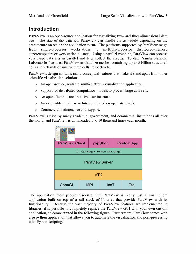
MPIOpenGL IceT Etc.
VTK
ParaView Server
ParaView Client pvpython Custom App
UI (Qt Widgets, Python Wrappings)
The application most people associate with ParaView is really just a small client application built on top of a tall stack of libraries that provide ParaView with its functionality. Because the vast majority of ParaView features are implemented in libraries, it is possible to completely replace the ParaView GUI with your own custom application, as demonstrated in the following figure. Furthermore, ParaView comes with a pvpython application that allows you to automate the visualization and post-processing with Python scripting.
1

Moreland and Greenfield Large Scale Visualization with ParaView 3
Available to each ParaView application is a library of user interface components to maximize code sharing between them. A ParaView Server library provides the abstraction layer necessary for running parallel, interactive visualization. It relieves the client application from most of the issues concerning if and how ParaView is running in parallel. The Visualization Toolkit (VTK) provides the basic visualization and rendering algorithms. VTK incorporates several other libraries to provide basic functionalities such as rendering, parallel processing, file I/O, and parallel rendering. Although this tutorial demonstrates using ParaView through the ParaView client application, be aware that the modular design of ParaView allows for a great deal of flexibility and customization.
Development and Funding The ParaView project started in 2000 as a collaborative effort between Kitware Inc. and Los Alamos National Laboratory. The initial funding was provided by a three year contract with the US Department of Energy ASCI Views program. The first public release, ParaView 0.6, was announced in October 2002. Development of ParaView continued through collaboration of Kitware Inc. with Sandia National Laboratories, Los Alamos National Laboratories, the Army Research Laboratory, and various other academic and government institutions.
In September 2005, Kitware, Sandia National Labs and CSimSoft started the development of ParaView 3.0. This was a major effort focused on rewriting the user interface to be more user friendly and on developing a quantitative analysis framework. ParaView 3.0 was released in May 2007.
Development of ParaView continues today. Sandia National Laboratories continues to fund ParaView development through the ASC project. ParaView is integrated as the major development platform for SciDAC Institute for Ultra-Scale Visualization (www.ultravis.org). The US Department of Energy also funds ParaView through Los Alamos National Laboratories, an Army SBIR, and an ERDC contract. The US National Science Foundation also funds ParaView with an SBIR. Other institutions also have ParaView support contracts: Electricity de France, Mirarco, and oil industry customers. Also, because ParaView is an open source project, other institutions such as the Swiss National Supercomputing Centre contribute back their own development.
2

Moreland and Greenfield Large Scale Visualization with ParaView 3
Basics of Visualization
Put simply, the process of visualization is taking raw data and converting it to a form that is viewable and understandable to humans. This allows us to get a better cognitive understanding of our data. Scientific visualization is specifically concerned with the type of data that has a well defined representation in 2D or 3D space. Data that comes from simulation meshes and scanner data is well suited for this type of analysis.
There are three basic steps to visualizing your data: reading, filtering, and rendering. First, your data must be read into ParaView. Next, you may apply any number of filters that process the data to generate, extract, or derive features from the data. Finally, a viewable image is rendered from the data.
Because ParaView handles data with spatial representation, the basic data types used in ParaView are meshes.
Uniform Rectilinear (Image Data) A uniform rectilinear grid is a one- two- or three- dimensional array of data. The points are orthonormal to each other and are spaced regularly along each direction.
3
Moreland and Greenfield Large Scale Visualization with ParaView 3
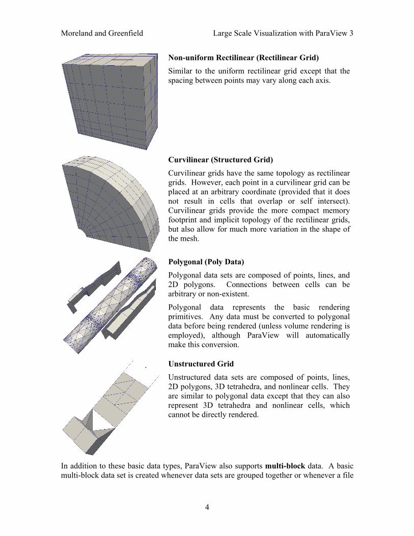
Non-uniform Rectilinear (Rectilinear Grid)
Similar to the uniform rectilinear grid except that the spacing between points may vary along each axis.
Curvilinear (Structured Grid) Curvilinear grids have the same topology as rectilinear grids. However, each point in a curvilinear grid can be placed at an arbitrary coordinate (provided that it does not result in cells that overlap or self intersect). Curvilinear grids provide the more compact memory footprint and implicit topology of the rectilinear grids, but also allow for much more variation in the shape of the mesh.
Polygonal (Poly Data) Polygonal data sets are composed of points, lines, and 2D polygons. Connections between cells can be arbitrary or non-existent.
Polygonal data represents the basic rendering primitives. Any data must be converted to polygonal data before being rendered (unless volume rendering is employed), although ParaView will automatically make this conversion.
Unstructured Grid Unstructured data sets are composed of points, lines, 2D polygons, 3D tetrahedra, and nonlinear cells. They are similar to polygonal data except that they can also represent 3D tetrahedra and nonlinear cells, which cannot be directly rendered.
In addition to these basic data types, ParaView also supports multi-block data. A basic multi-block data set is created whenever data sets are grouped together or whenever a file
4
Moreland and Greenfield Large Scale Visualization with ParaView 3
containing multiple blocks is read. ParaView also has some special data types for representing Hierarchical Adaptive Mesh Refinement (AMR), Hierarchical Uniform AMR, and Octree data sets.
More Information There are many places to find more information about ParaView. For starters, ParaView has online help that can be accessed by simply clicking the button in the application. In addition to the on-line help, The ParaView Guide written by Amy Henderson Squillacote is a helpful guide for all things ParaView. It is available from Kitware, and a new version updated for ParaView 3 should be available “real soon now.”
The ParaView web page, www.paraview.org, is also an excellent place to find more information about ParaView. From there you can find helpful links to mailing lists, Wiki pages, and frequently asked questions as well as information about professional support services.
5
Moreland and Greenfield Large Scale Visualization with ParaView 3
Basic Usage Let us get started using ParaView. In order to follow along, you will need your own installation of ParaView. If you do not already have ParaView, you can download a copy from http://www.paraview.org/New/download.html. ParaView launches like most other applications. On Windows, the launcher is located in the start menu. On Macintosh, open the application bundle that you installed. On Linux, execute paraview from a command prompt (you may need to set your path).
The examples in this tutorial also rely on some data that is available at http://www.paraview.org/Wiki/SC07_ParaView_Tutorial. You may install this data into any directory that you like, but make sure that you can find that directory easily. Any time the tutorial asks you to load a file it will be from the directory you installed this data in.
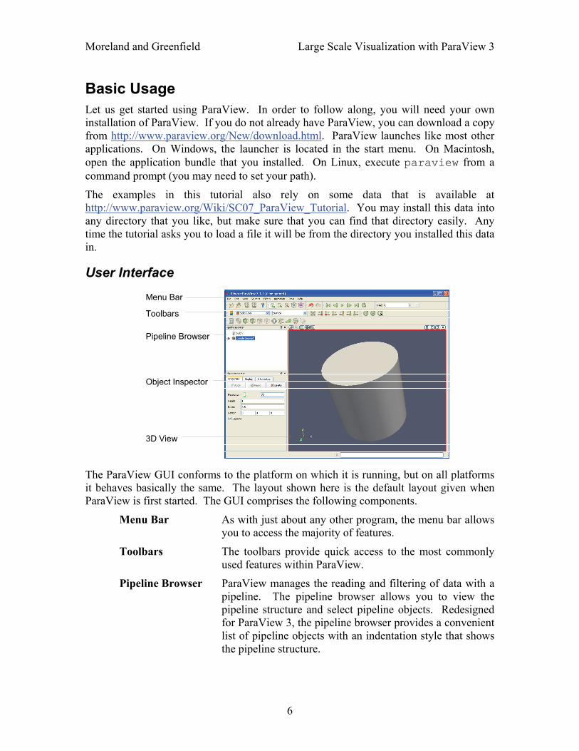
User Interface
Menu Bar
Toolbars
Pipeline Browser
Object Inspector
3D View
The ParaView GUI conforms to the platform on which it is running, but on all platforms it behaves basically the same. The layout shown here is the default layout given when ParaView is first started. The GUI comprises the following components.
Menu Bar As with just about any other program, the menu bar allows you to access the majority of features.
Toolbars The toolbars provide quick access to the most commonly used features within ParaView.
Pipeline Browser ParaView manages the reading and filtering of data with a pipeline. The pipeline browser allows you to view the pipeline structure and select pipeline objects. Redesigned for ParaView 3, the pipeline browser provides a convenient list of pipeline objects with an indentation style that shows the pipeline structure.
6
Moreland and Greenfield Large Scale Visualization with ParaView 3
Object Inspector The object inspector allows you to view and change the parameters of the current pipeline object. There are three tabs in the object inspector. The Properties tab presents the configurable options for the object behavior. The Display tab presents options for how the object is represented in the view. The Information tab shows basic statistics on the data produced by the pipeline object.
3D View The remainder of the GUI is used to present data so that you may view, interact with, and explore your data. This area is initially populated with a 3D view that will provide a geometric representation of the data.
Note that the GUI layout is highly configurable, so that it is easy to change the look of the window. The toolbars can be moved around and even hidden from view. To toggle the use of a toolbar, use the View → Toolbars submenu. The pipeline browser and object inspector are both dockable windows. This means that these components can be moved around in the GUI, torn off as their own floating windows, or hidden altogether. These two windows are important to the operation of ParaView, so if you hide them and then need them again, you can get them back with the View menu.
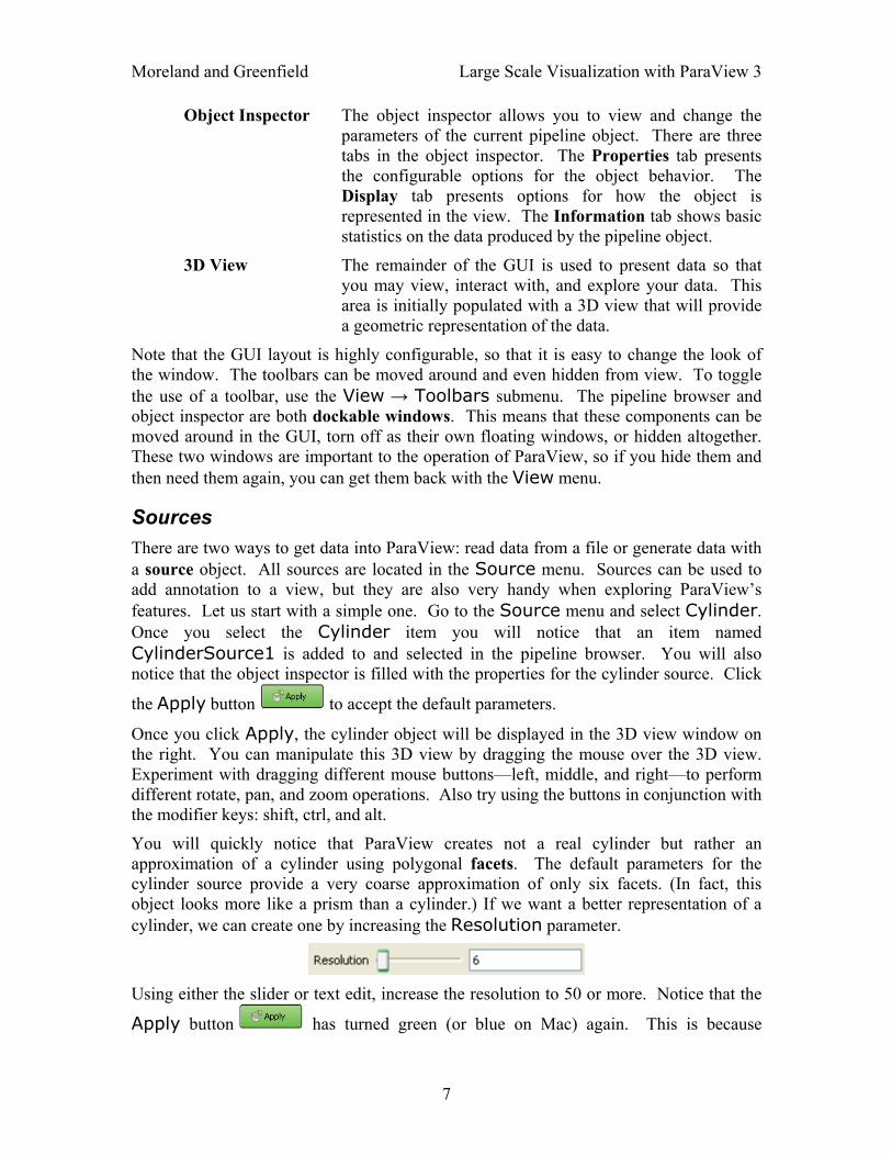
Sources There are two ways to get data into ParaView: read data from a file or generate data with a source object. All sources are located in the Source menu. Sources can be used to add annotation to a view, but they are also very handy when exploring ParaView’s features. Let us start with a simple one. Go to the Source menu and select Cylinder. Once you select the Cylinder item you will notice that an item named CylinderSource1 is added to and selected in the pipeline browser. You will also notice that the object inspector is filled with the properties for the cylinder source. Click
the Apply button to accept the default parameters.
Once you click Apply, the cylinder object will be displayed in the 3D view window on the right. You can manipulate this 3D view by dragging the mouse over the 3D view. Experiment with dragging different mouse buttons—left, middle, and right—to perform different rotate, pan, and zoom operations. Also try using the buttons in conjunction with the modifier keys: shift, ctrl, and alt.
You will quickly notice that ParaView creates not a real cylinder but rather an approximation of a cylinder using polygonal facets. The default parameters for the cylinder source provide a very coarse approximation of only six facets. (In fact, this object looks more like a prism than a cylinder.) If we want a better representation of a cylinder, we can create one by increasing the Resolution parameter.
Using either the slider or text edit, increase the resolution to 50 or more. Notice that the
Apply button has turned green (or blue on Mac) again. This is because
7
Moreland and Greenfield Large Scale Visualization with ParaView 3
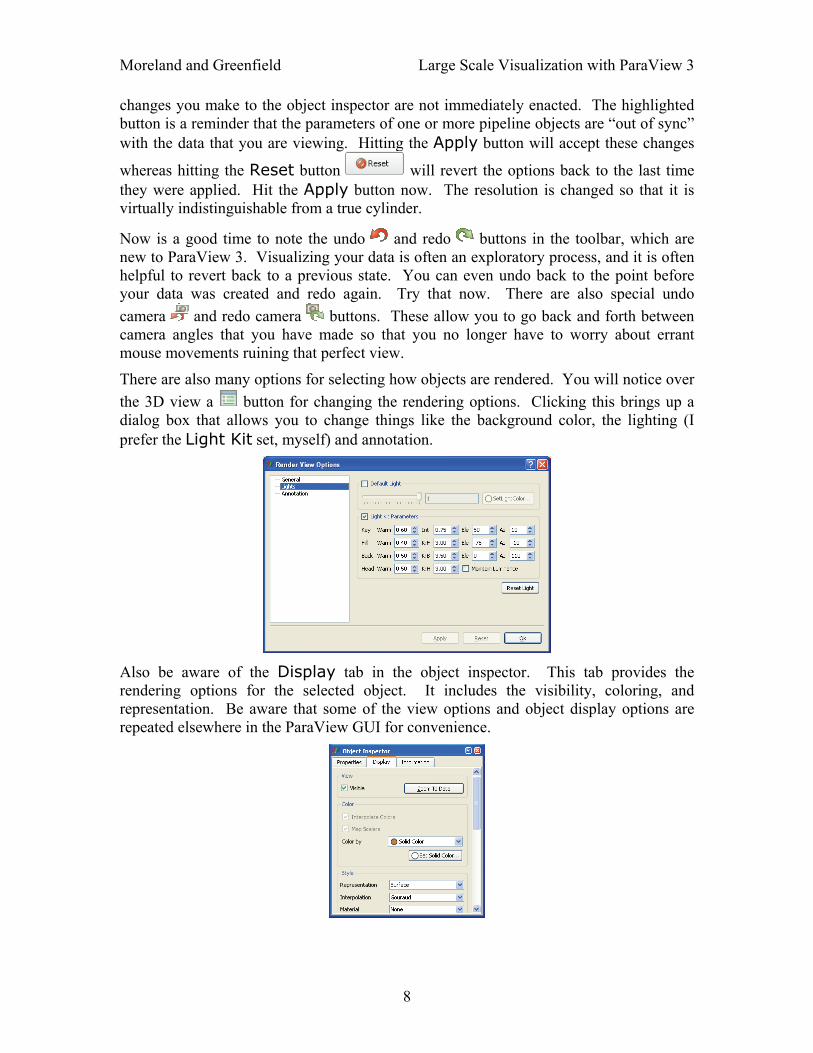
changes you make to the object inspector are not immediately enacted. The highlighted button is a reminder that the parameters of one or more pipeline objects are “out of sync” with the data that you are viewing. Hitting the Apply button will accept these changes
whereas hitting the Reset button will revert the options back to the last time they were applied. Hit the Apply button now. The resolution is changed so that it is virtually indistinguishable from a true cylinder.
Now is a good time to note the undo and redo buttons in the toolbar, which are new to ParaView 3. Visualizing your data is often an exploratory process, and it is often helpful to revert back to a previous state. You can even undo back to the point before your data was created and redo again. Try that now. There are also special undo camera and redo camera buttons. These allow you to go back and forth between camera angles that you have made so that you no longer have to worry about errant mouse movements ruining that perfect view.
There are also many options for selecting how objects are rendered. You will notice over the 3D view a button for changing the rendering options. Clicking this brings up a dialog box that allows you to change things like the background color, the lighting (I prefer the Light Kit set, myself) and annotation.
Also be aware of the Display tab in the object inspector. This tab provides the rendering options for the selected object. It includes the visibility, coloring, and representation. Be aware that some of the view options and object display options are repeated elsewhere in the ParaView GUI for convenience.
8
Moreland and Greenfield Large Scale Visualization with ParaView 3
We are done with the cylinder source now. We can delete the pipeline object by
selecting the Properties tab and hitting delete in the object inspector.
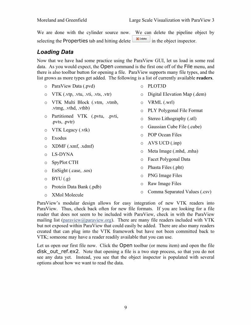
Loading Data Now that we have had some practice using the ParaView GUI, let us load in some real data. As you would expect, the Open command is the first one off of the File menu, and there is also toolbar button for opening a file. ParaView supports many file types, and the list grows as more types get added. The following is a list of currently available readers.
o ParaView Data (.pvd)
o VTK (.vtp, .vtu, .vti, .vts, .vtr)
o VTK Multi Block (.vtm, .vtmb, .vtmg, .vthd, .vthb)
o Partitioned VTK (.pvtu, .pvti, .pvts, .pvtr)
o VTK Legacy (.vtk)
o Exodus
o XDMF (.xmf, .xdmf)
o LS-DYNA
o SpyPlot CTH
o EnSight (.case, .sos)
o BYU (.g)
o Protein Data Bank (.pdb)
o XMol Molecule
o PLOT3D
o Digital Elevation Map (.dem)
o VRML (.wrl)
o PLY Polygonal File Format
o Stereo Lithography (.stl)
o Gaussian Cube File (.cube)
o POP Ocean Files
o AVS UCD (.inp)
o Meta Image (.mhd, .mha)
o Facet Polygonal Data
o Phasta Files (.pht)
o PNG Image Files
o Raw Image Files
o Comma Separated Values (.csv)
ParaView’s modular design allows for easy integration of new VTK readers into ParaView. Thus, check back often for new file formats. If you are looking for a file reader that does not seem to be included with ParaView, check in with the ParaView mailing list ([email protected]). There are many file readers included with VTK but not exposed within ParaView that could easily be added. There are also many readers created that can plug into the VTK framework but have not been committed back to VTK; someone may have a reader readily available that you can use.
Let us open our first file now. Click the Open toolbar (or menu item) and open the file disk_out_ref.ex2. Note that opening a file is a two step process, so that you do not see any data yet. Instead, you see that the object inspector is populated with several options about how we want to read the data.
9
Moreland and Greenfield Large Scale Visualization with ParaView 3
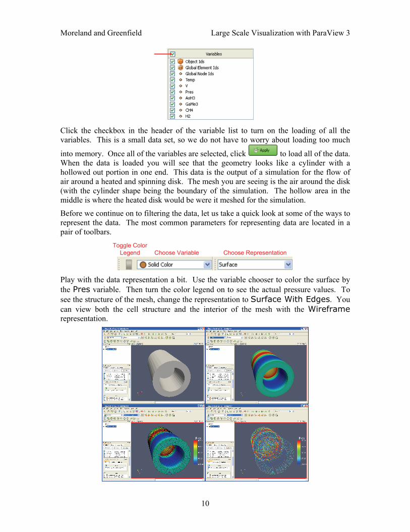
Click the checkbox in the header of the variable list to turn on the loading of all the variables. This is a small data set, so we do not have to worry about loading too much
into memory. Once all of the variables are selected, click to load all of the data. When the data is loaded you will see that the geometry looks like a cylinder with a hollowed out portion in one end. This data is the output of a simulation for the flow of air around a heated and spinning disk. The mesh you are seeing is the air around the disk (with the cylinder shape being the boundary of the simulation. The hollow area in the middle is where the heated disk would be were it meshed for the simulation.
Before we continue on to filtering the data, let us take a quick look at some of the ways to represent the data. The most common parameters for representing data are located in a pair of toolbars.
Toggle ColorLegend Choose Variable Choose Representation
Play with the data representation a bit. Use the variable chooser to color the surface by the Pres variable. Then turn the color legend on to see the actual pressure values. To see the structure of the mesh, change the representation to Surface With Edges. You can view both the cell structure and the interior of the mesh with the Wireframe representation.
10
Moreland and Greenfield Large Scale Visualization with ParaView 3
Filters We have now successfully read in some data and gleaned some information about it. We can see the basic structure of the mesh and map some data onto the surface of the mesh. However, as we will soon see, there are many interesting features about this data that we cannot determine by simply looking at the surface of this data. There are many variables associated with the mesh of different types (scalars and vectors). And remember that the mesh is a solid model. Most of the interesting information is on the inside.
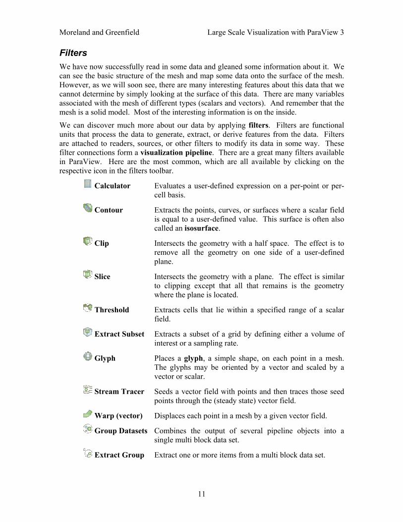
We can discover much more about our data by applying filters. Filters are functional units that process the data to generate, extract, or derive features from the data. Filters are attached to readers, sources, or other filters to modify its data in some way. These filter connections form a visualization pipeline. There are a great many filters available in ParaView. Here are the most common, which are all available by clicking on the respective icon in the filters toolbar.
Calculator Evaluates a user-defined expression on a per-point or per-cell basis.
Contour Extracts the points, curves, or surfaces where a scalar field is equal to a user-defined value. This surface is often also called an isosurface.
Clip Intersects the geometry with a half space. The effect is to remove all the geometry on one side of a user-defined plane.
Slice Intersects the geometry with a plane. The effect is similar to clipping except that all that remains is the geometry where the plane is located.
Threshold Extracts cells that lie within a specified range of a scalar field.
Extract Subset Extracts a subset of a grid by defining either a volume of interest or a sampling rate.
Glyph Places a glyph, a simple shape, on each point in a mesh. The glyphs may be oriented by a vector and scaled by a vector or scalar.
Stream Tracer Seeds a vector field with points and then traces those seed points through the (steady state) vector field.
Warp (vector) Displaces each point in a mesh by a given vector field.
Group Datasets Combines the output of several pipeline objects into a single multi block data set.
Extract Group Extract one or more items from a multi block data set.
11

Moreland and Greenfield Large Scale Visualization with ParaView 3
These eleven filters are a small sampling of what is available in ParaView. In the Filters menu are a great many more filters that you can use to process your data. ParaView currently exposes over eighty filters, so to make them easier to find the Filters menu is organized into submenus. These submenus are organized as follows.
Recent The list of most recently used filters sorted with the most recently used filters on top.
Common The most common filters. This is the same list of filters available in the filters toolbar and listed previously.
Data Analysis The filters designed to retrieve quantitative values from the data. These filters compute data on the mesh, extract elements from the mesh, or plot data.
Alphabetical An alphabetical listing of all the filters available. If you are not sure where to find a particular filter, this list is guaranteed to have it. There are also many filters that are not listed anywhere but in this list.
You have probably noticed that some of the filters are grayed out. Many filters only work on a specific types of data and therefore cannot always be used. ParaView disables these filters from the menu and toolbars to indicate (and enforce) that you cannot use these filters.
Throughout this tutorial we will explore many filters. However, we cannot explore all the filters in this forum. Consult The ParaView Guide for more information on each filter.
Let us apply our first filter. Make sure that disk_out_ref.ex2 is selected in the pipeline browser and then select the contour filter from the filter toolbar or Filters menu. Notice that a new item is added to the pipeline filter underneath the reader and the object inspector updates to the parameters of the new filter. As with reading a file, applying a filter is a two step process. After creating the filter you get a chance to modify the parameters (which you will almost always do) before applying the filter.
12
Moreland and Greenfield Large Scale Visualization with ParaView 3
Change to Temp
Change to 400
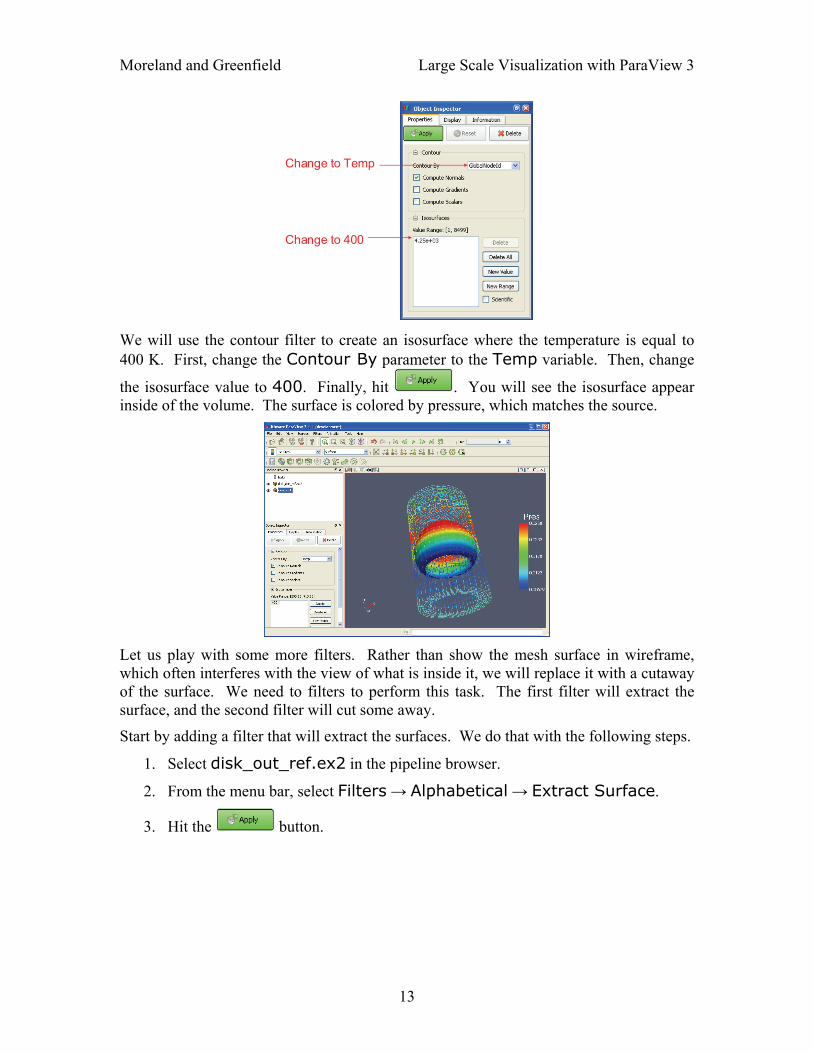
We will use the contour filter to create an isosurface where the temperature is equal to 400 K. First, change the Contour By parameter to the Temp variable. Then, change
the isosurface value to 400. Finally, hit . You will see the isosurface appear inside of the volume. The surface is colored by pressure, which matches the source.
Let us play with some more filters. Rather than show the mesh surface in wireframe, which often interferes with the view of what is inside it, we will replace it with a cutaway of the surface. We need to filters to perform this task. The first filter will extract the surface, and the second filter will cut some away.
Start by adding a filter that will extract the surfaces. We do that with the following steps.
1. Select disk_out_ref.ex2 in the pipeline browser.
2. From the menu bar, select Filters → Alphabetical → Extract Surface.
3. Hit the button.
13
Moreland and Greenfield Large Scale Visualization with ParaView 3
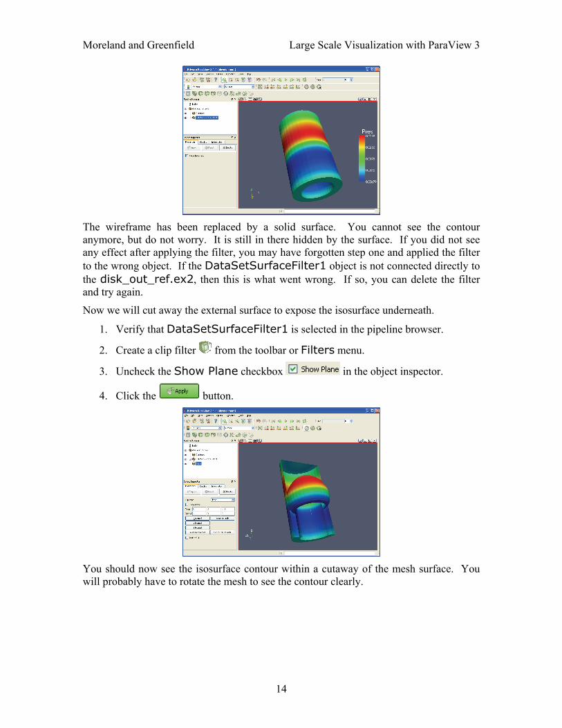
The wireframe has been replaced by a solid surface. You cannot see the contour anymore, but do not worry. It is still in there hidden by the surface. If you did not see any effect after applying the filter, you may have forgotten step one and applied the filter to the wrong object. If the DataSetSurfaceFilter1 object is not connected directly to the disk_out_ref.ex2, then this is what went wrong. If so, you can delete the filter and try again.
Now we will cut away the external surface to expose the isosurface underneath.
1. Verify that DataSetSurfaceFilter1 is selected in the pipeline browser.
2. Create a clip filter from the toolbar or Filters menu.
3. Uncheck the Show Plane checkbox in the object inspector.
4. Click the button.
You should now see the isosurface contour within a cutaway of the mesh surface. You will probably have to rotate the mesh to see the contour clearly.
14

Moreland and Greenfield Large Scale Visualization with ParaView 3
Disk_out_ref.ex2
Contour1DataSetSurfaceFilter1
Clip1
Now that we have added several filters to our pipeline, let us take a look at the layout of these filters in the pipeline browser. The pipeline browser provides a convenient list of pipeline objects that we have created make it easy to select pipeline objects and change their visibility by clicking on the eyeball icons next to them. But also notice the indentation of the entries in the list and the connecting lines toward the right. These features reveal the connectivity of the pipeline. It shows the same information as the traditional graph layout on the right, but in a much more compact space. The trouble with the traditional layout of pipeline objects is that it takes a lot of space, and even moderately sized pipelines require a significant portion of the GUI to see fully. The pipeline browser, however, is complete and compact.
Multiview Occasionally in the pursuit of science we can narrow our focus down to one variable. However, most interesting physical phenomena rely on not one but many variables interacting in certain ways. It can be very challenging to present many variables in the same view. To help you explore complicated visualization data, ParaView contains the ability to present multiple views of data and correlate them together.
So far in our visualization we are looking at two variables: We are coloring with pressure and have extracted an isosurface with temperature. Although we are starting to get the feel for the layout of these variables, it is still difficult to make correlations between them. To make this correlation easier, we can use multiple views. Each view can show an independent aspect of the data and together they may show a more complete understanding.
On top of each view is a small toolbar, and the buttons controlling the creating and deletion of views are located on the right side of this tool bar. There are four buttons in all. You can create a new view by splitting an existing view horizontally or vertically with the and buttons, respectively. The button deletes a view, whose space is consumed by an adjacent view. The temporarily fills view space with the selected view until is pressed. Press the button now.
15
Moreland and Greenfield Large Scale Visualization with ParaView 3
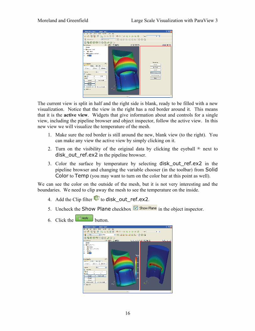
The current view is split in half and the right side is blank, ready to be filled with a new visualization. Notice that the view in the right has a red border around it. This means that it is the active view. Widgets that give information about and controls for a single view, including the pipeline browser and object inspector, follow the active view. In this new view we will visualize the temperature of the mesh.
1. Make sure the red border is still around the new, blank view (to the right). You can make any view the active view by simply clicking on it.
2. Turn on the visibility of the original data by clicking the eyeball next to disk_out_ref.ex2 in the pipeline browser.
3. Color the surface by temperature by selecting disk_out_ref.ex2 in the pipeline browser and changing the variable chooser (in the toolbar) from Solid Color to Temp (you may want to turn on the color bar at this point as well).
We can see the color on the outside of the mesh, but it is not very interesting and the boundaries. We need to clip away the mesh to see the temperature on the inside.
4. Add the Clip filter to disk_out_ref.ex2.
5. Uncheck the Show Plane checkbox in the object inspector.
6. Click the button.
16

Moreland and Greenfield Large Scale Visualization with ParaView 3
We now have two views: one showing information about pressure and the other information about temperature. We would like to compare these, but it is difficult to do because the orientations are different. How are we to know how a location in one correlates to a location in the other. We can solve this problem by adding a camera link so that the two views will always be drawn from the same viewpoint. Linking cameras is easy. First right click on one of the views and select Link Camera… from the pop up menu. (If you are on a Mac with no right mouse button, you can perform the same operation with the menu option Tools → Add Camera Link…) Now click in a second view. Viola! The two cameras are linked; each will follow the other.
With the cameras linked, we can make some comparisons between the two views. Click the button to get a straight-on view of the cross section. Notice that the temperature is highest at the interface with the heated disk. That alone is not surprising. We expect the air temperature to be greatest near the heat source and drop off away from it. But notice that at the same position the pressure is not maximal. The air pressure is maximal at a position above the disk. Based on this information we can draw some interesting hypotheses about the physical phenomenon. We can expect that there are two forces contributing to air pressure. The first force is that of gravity causing the upper air to press down on the lower air. The second force is that of the heated air becoming less dense and therefore rising. We can see based on the maximal pressure where these two forces are equal. Such an observation cannot be drawn without looking at both the temperature and pressure in this way.
Multiview in ParaView is of course not limited to simply two windows. Note that each of the views has its own set of multiview buttons. You can create more views by using the split view buttons to arbitrarily divide up the working space. And you can delete views at any time.
17
Moreland and Greenfield Large Scale Visualization with ParaView 3
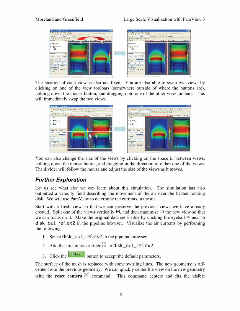
The location of each view is also not fixed. You are also able to swap two views by clicking on one of the view toolbars (somewhere outside of where the buttons are), holding down the mouse button, and dragging onto one of the other view toolbars. This will immediately swap the two views.
You can also change the size of the views by clicking on the space in between views, holding down the mouse button, and dragging in the direction of either one of the views. The divider will follow the mouse and adjust the size of the views as it moves.
Further Exploration Let us see what else we can learn about this simulation. The simulation has also outputted a velocity field describing the movement of the air over the heated rotating disk. We will use ParaView to determine the currents in the air.
Start with a fresh view so that we can preserve the previous views we have already created. Split one of the views vertically , and then maximize the new view so that we can focus on it. Make the original data set visible by clicking the eyeball next to disk_out_ref.ex2 in the pipeline browser. Visualize the air currents by performing the following.
1. Select disk_out_ref.ex2 in the pipeline browser.
2. Add the stream tracer filter to disk_out_ref.ex2.
3. Click the button to accept the default parameters.
The surface of the mesh is replaced with some swirling lines. The new geometry is off-center from the previous geometry. We can quickly center the view on the new geometry with the reset camera command. This command centers and fits the visible
18
Moreland and Greenfield Large Scale Visualization with ParaView 3
geometry within the current view and also resets the center of rotation to the middle of the visible geometry.
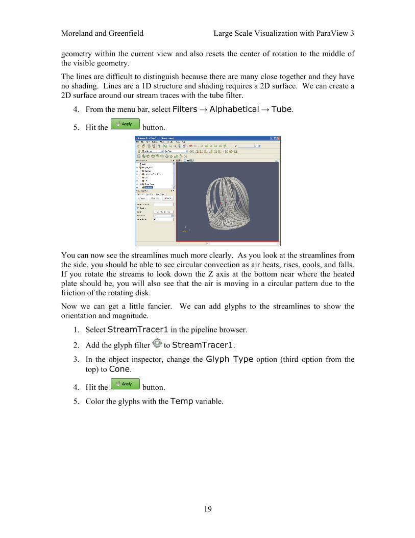
The lines are difficult to distinguish because there are many close together and they have no shading. Lines are a 1D structure and shading requires a 2D surface. We can create a 2D surface around our stream traces with the tube filter.
4. From the menu bar, select Filters → Alphabetical → Tube.
5. Hit the button.
You can now see the streamlines much more clearly. As you look at the streamlines from the side, you should be able to see circular convection as air heats, rises, cools, and falls. If you rotate the streams to look down the Z axis at the bottom near where the heated plate should be, you will also see that the air is moving in a circular pattern due to the friction of the rotating disk.
Now we can get a little fancier. We can add glyphs to the streamlines to show the orientation and magnitude.
1. Select StreamTracer1 in the pipeline browser.
2. Add the glyph filter to StreamTracer1.
3. In the object inspector, change the Glyph Type option (third option from the top) to Cone.
4. Hit the button.
5. Color the glyphs with the Temp variable.
19

Moreland and Greenfield Large Scale Visualization with ParaView 3
Now the streamlines are augmented with little pointers. The pointers face in the direction of the velocity, and their size is proportional to the magnitude of the velocity. Try using this new information to answer the following questions.
o Where is the air moving the fastest? Near the disk or away from it? At the center of the disk or near its edges?
o Which way is the plate spinning?
o At the surface of the disk, is air moving toward the center or away from it?
When you are done, you can restore all of your views by pressing the restore button on the view toolbar. Right click on the new view and select Link Camera… and then link the camera with either of the other two views. Now all three views have their cameras linked together.
Selection A feature that greatly improved with the release of ParaView 3 is that of selection. Selection can take place at any time, and ParaView maintains a current selected set that is linked between all views. That is, if you select something in one view, that selection is also shown in all other views that display the same object.
ParaView currently supports four different types of selection. All the selections allow you to perform a rubber-band selection. The selection types differ in which elements under the rubber band are selected.
Surface Cell Selection Selects cells that are visible in the view.
Surface Point Selection Selects points that are visible in the view.
Through Cell Selection Selects all cells that exist under the rubber band.
Through Point Selection Selects all points that exist under the rubber band.
Experiment with the selections now.
20

Moreland and Greenfield Large Scale Visualization with ParaView 3
You can manage your selection with the selection inspector. You can view the selection inspector through the menu View → Selection Inspector. The selection inspector allows you to view all the points and cells in the selection as well as modify the selection. You can also use the selection inspector to add labels to the selection to make it easier to identify which element is which.
You can also extract a selection in order to view the selected points or cells separately or perform some independent processing on them. This is done through the Extract Selections filter. Try this.
1. Perform a through cell selection on one of the objects in one of your views.
2. Make sure that the object you selected on is also selected in the pipeline browser.
3. From the menu bar, select Filters → Data Analysis → Extract Selection.
4. Click the Copy Active Selection button in the object inspector.
5. Hit the button.
The object in the view is replaced with the cells that you just selected. (Note that in this image I added a translucent surface to show the extracted cells in relation to the original data.) You can perform computations on the extracted cells by simply adding filters to the extract selection pipeline object. We are done with the extracted cells, so delete them.
6. Hit the button to delete the ExtractSurface1 pipeline object.
21

Moreland and Greenfield Large Scale Visualization with ParaView 3
Volume Rendering ParaView has several ways to represent data. We have already seen some examples: surfaces, wireframe, and a combination of both. ParaView can also render the points on the surface or simply draw a bounding box of the data.
A powerful way that ParaView lets you represent your data is with a technique called volume rendering. With volume rendering, a solid mesh is rendered as a translucent cloud with the scalar field determining the color and density at every point in the cloud. Unlike with surface rendering, volume rendering allows you to see features all the way through a volume.
Volume rendering is enabled by simply changing the representation of the object. Let us replace the view of the temperature with a volume rendering of the data.
1. Select the view showing the temperature on the surface of the clipped mesh.
2. Delete the clip filter that is visible. First select the filter in the pipeline and then
hit the button. The clipped mesh will be replaced with the full solid mesh (disk_out_ref.ex2).
3. Make sure disk_out_ref.ex2 is selected in the pipeline browser. Change the variable viewed to Temp and change the representation to Volume.
The solid opaque mesh is replaced with a translucent volume. You may notice that when rotating the image is temporarily replaced with a simpler image for performance reasons, we will discuss this feature in more detail later. A useful feature of ParaView’s volume rendering is that it can be mixed with the surface rendering of other objects. This allows you to add context to the volume rendering or to mix visualizations for a more information-rich view. For example, we can add a volume rendering of the temperature to the view containing the streamlines.
1. Select the view showing the streamlines.
2. Click on the next to disk_out_ref.ex2 in the pipeline browser to make it visible and also click on the label disk_out_ref.ex2 itself to select that object.
3. Change the variable viewed to Temp and change the representation to Volume.
22
Moreland and Greenfield Large Scale Visualization with ParaView 3
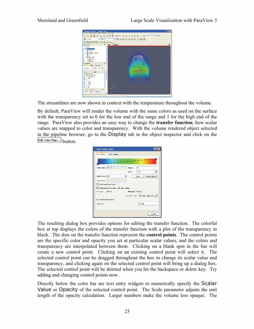
The streamlines are now shown in context with the temperature throughout the volume.
By default, ParaView will render the volume with the same colors as used on the surface with the transparency set to 0 for the low end of the range and 1 for the high end of the range. ParaView also provides an easy way to change the transfer function, how scalar values are mapped to color and transparency. With the volume rendered object selected in the pipeline browser, go to the Display tab in the object inspector and click on the
button.
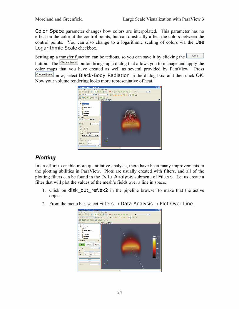
The resulting dialog box provides options for editing the transfer function. The colorful box at top displays the colors of the transfer function with a plot of the transparency in black. The dots on the transfer function represent the control points. The control points are the specific color and opacity you set at particular scalar values, and the colors and transparency are interpolated between them. Clicking on a blank spot in the bar will create a new control point. Clicking on an existing control point will select it. The selected control point can be dragged throughout the box to change its scalar value and transparency, and clicking again on the selected control point will bring up a dialog box. The selected control point will be deleted when you hit the backspace or delete key. Try adding and changing control points now.
Directly below the color bar are text entry widgets to numerically specify the Scalar Value or Opacity of the selected control point. The Scale parameter adjusts the unit length of the opacity calculation. Larger numbers make the volume less opaque. The
23
Moreland and Greenfield Large Scale Visualization with ParaView 3
Color Space parameter changes how colors are interpolated. This parameter has no effect on the color at the control points, but can drastically affect the colors between the control points. You can also change to a logarithmic scaling of colors via the Use Logarithmic Scale checkbox.
Setting up a transfer function can be tedious, so you can save it by clicking the button. The button brings up a dialog that allows you to manage and apply the color maps that you have created as well as several provided by ParaView. Press
now, select Black-Body Radiation in the dialog box, and then click OK. Now your volume rendering looks more representative of heat.
Plotting In an effort to enable more quantitative analysis, there have been many improvements to the plotting abilities in ParaView. Plots are usually created with filters, and all of the plotting filters can be found in the Data Analysis submenu of Filters. Let us create a filter that will plot the values of the mesh’s fields over a line in space.
1. Click on disk_out_ref.ex2 in the pipeline browser to make that the active object.
2. From the menu bar, select Filters → Data Analysis → Plot Over Line.
24
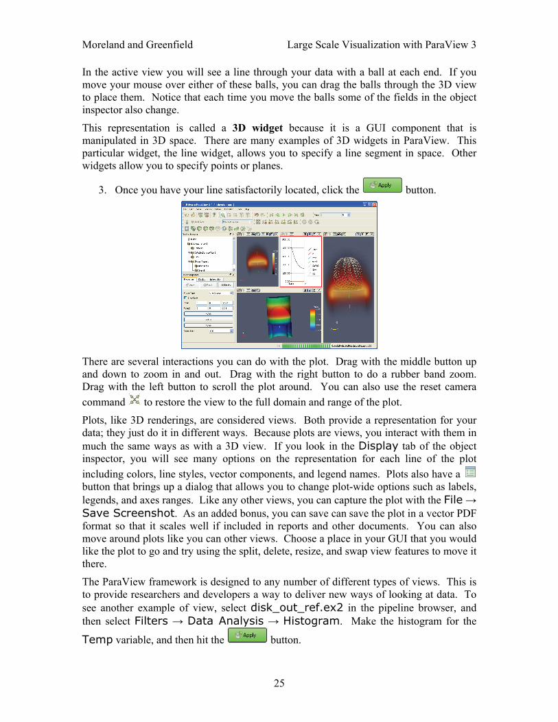
Moreland and Greenfield Large Scale Visualization with ParaView 3
In the active view you will see a line through your data with a ball at each end. If you move your mouse over either of these balls, you can drag the balls through the 3D view to place them. Notice that each time you move the balls some of the fields in the object inspector also change.
This representation is called a 3D widget because it is a GUI component that is manipulated in 3D space. There are many examples of 3D widgets in ParaView. This particular widget, the line widget, allows you to specify a line segment in space. Other widgets allow you to specify points or planes.
3. Once you have your line satisfactorily located, click the button.
There are several interactions you can do with the plot. Drag with the middle button up and down to zoom in and out. Drag with the right button to do a rubber band zoom. Drag with the left button to scroll the plot around. You can also use the reset camera command to restore the view to the full domain and range of the plot.
Plots, like 3D renderings, are considered views. Both provide a representation for your data; they just do it in different ways. Because plots are views, you interact with them in much the same ways as with a 3D view. If you look in the Display tab of the object inspector, you will see many options on the representation for each line of the plot including colors, line styles, vector components, and legend names. Plots also have a button that brings up a dialog that allows you to change plot-wide options such as labels, legends, and axes ranges. Like any other views, you can capture the plot with the File → Save Screenshot. As an added bonus, you can save can save the plot in a vector PDF format so that it scales well if included in reports and other documents. You can also move around plots like you can other views. Choose a place in your GUI that you would like the plot to go and try using the split, delete, resize, and swap view features to move it there.
The ParaView framework is designed to any number of different types of views. This is to provide researchers and developers a way to deliver new ways of looking at data. To see another example of view, select disk_out_ref.ex2 in the pipeline browser, and then select Filters → Data Analysis → Histogram. Make the histogram for the
Temp variable, and then hit the button.
25
Moreland and Greenfield Large Scale Visualization with ParaView 3
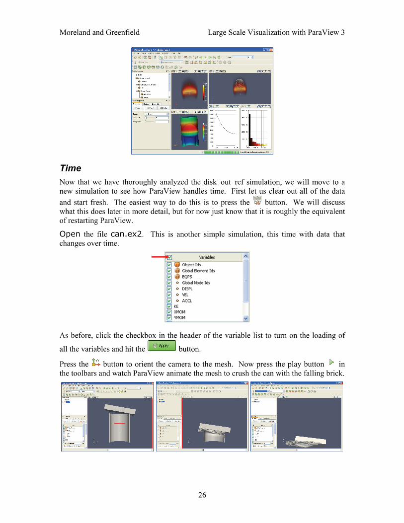
Time Now that we have thoroughly analyzed the disk_out_ref simulation, we will move to a new simulation to see how ParaView handles time. First let us clear out all of the data and start fresh. The easiest way to do this is to press the button. We will discuss what this does later in more detail, but for now just know that it is roughly the equivalent of restarting ParaView.
Open the file can.ex2. This is another simple simulation, this time with data that changes over time.
As before, click the checkbox in the header of the variable list to turn on the loading of
all the variables and hit the button.
Press the button to orient the camera to the mesh. Now press the play button in the toolbars and watch ParaView animate the mesh to crush the can with the falling brick.
26

Moreland and Greenfield Large Scale Visualization with ParaView 3
That is really all there is to dealing with data that is defined over time. ParaView has an internal concept of time and automatically links in the time defined by your data. Become familiar with the toolbars that can be used to control time.
FirstFrame
PreviousFrame Play Next
FrameLast
FrameLoop
AnimationCurrent
TimeCurrent
Time Step
Saving an animation is equally as easy. From the menu, select File → Save Animation. ParaView provides dialogs specifying how you want to save the animation, and then automatically iterates and saves the animation.
The biggest pitfall users run into is that with mapping a set of colors whose range changes over time. To demonstrate this, go to the first time step , turn on the EQPS variable, and then turn on the color legend . Now play through the animation (or skip to the last time step ). The coloring is now not very useful. To quickly fix the problem, go to the Display tab in the object inspector and click on the Rescale to Data Range button.
Although this seems like a bug, it is not. It is the consequence of two unavoidable behaviors. First, when you turn on the visibility of a scalar field, the range of the field is set to the range of values in the current time step. Ideally, the range would be set to the max and min over all time steps in the data. However, that would require ParaView to load in all of the data on the initial read, and that would be prohibitively slow for large data. Second, when you animate over time, it is important to hold the color range fixed even if the range in the data changes. Changing the scale of the data as an animation plays causes a misrepresentation of the data. It is far better to let the scalars go out of the original color maps range than to imply that they have not. To get around the problem, simply go to a representative time step and hit or open the edit color scale dialog box and specify a range for the data.
ParaView has many powerful options for controlling time and animation. The majority of these are accessed through the animation view. From the menu, click on View → Animation View.
For now we will examine the controls at the top of the animation view. The animation mode parameter determines how ParaView will step through time during playback. There are three modes available.
Sequence Given a start and end time, break the animation into a specified number of frames spaced equally apart.
27
Moreland and Greenfield Large Scale Visualization with ParaView 3
Real Time ParaView will play back the animation such that it lasts the specified number of seconds. The actual number of frames created depends on the update time between frames.
Snap To TimeSteps ParaView will play back exactly those time steps that are defined by your data.
Whenever you load a file that contains time, ParaView will automatically change the animation mode to Snap To TimeSteps. Thus, by default you can load in your data, hit play , and see each time step as defined in your data. This is by far the most common use case.
A counter use case can occur when a simulation writes data at variable time intervals. Perhaps you would like the animation to play back relative to the simulation time rather than the time index. No problem. We can switch to one of the other two animation modes. Another use case is the desire to change the playback rate. Perhaps you would like to speed up or slow down the animation. The other two animation modes allow us to do that.
Try it now. Change the animation mode to Real Time. By default the animation is set up with the time range specified by the data and a duration of 10 seconds. Play the animation now. The result looks similar, but the animation is now a linear scaling of the simulation time and will complete in 10 seconds.
Now try changing the Duration to 30 seconds. The animation is clearly playing back more slowly. Unless your computer is updating slowly, you will also notice that the animation is jerkier than before. This is because we have exceeded the temporal resolution of the data set. Often this is the desired behavior; it is showing you exactly what is present in the data. However, if you wanted to make an animation for a presentation, you may want a smoother animation.
There is a special filter in ParaView to make this possible. It is called the temporal interpolator. This filter will interpolate the positional and field data in between the time steps defined in the original data set. This functionality is made possible by recent advances in the ParaView and VTK pipeline structure. Try the filter now. With can.ex2 highlighted in the pipeline browser, select Filters → Alphabetical →
Temporal Interpolator. Hit and change back to Real Time mode in the animation view if necessary. Play the animation to see the effect.
Text Annotation When using ParaView as a communication tool it is often helpful to annotate the images you create with text. With ParaView 3 it is very easy to create text annotation wherever you want in a 3D view. There is a special text source that simply places some text in the view. Try it now.
1. From the menu bar, select Sources → Text.
2. In the text edit box of the object inspector, type a message.
28

Moreland and Greenfield Large Scale Visualization with ParaView 3
3. Hit the button.
The text you entered appears in the 3D view. You can place this text wherever you want by simply dragging it with the mouse. The Display tab in the object inspector provides additional options for the size, font, and color of the text. It also has additional controls for placing the text in the most common locations.
Often times you will need to put the current time value into the text annotation. Typing the correct time value can be tedious an error prone with the standard text source and impossible when making an animation. Therefore, there is a special annotate time source that will insert the current animation time into the string.
29

Moreland and Greenfield Large Scale Visualization with ParaView 3
There are instances when the current animation time is not the same as the time step read from a data file. Often it is important to know what the time stored in the data file is, and there is a special version of annotate time that acts as a filter. It can be accessed from Filters → Alphabetical → Annotate Time.
Animations We have already seen how to animate a data set with time in it (hit ). However, ParaView’s animation capabilities go far beyond that. With ParaView you can animate nearly any property of any pipeline object. We will demonstrate that now, but first press the button to clear out the current ParaView state. Now we are ready to make a simple animation.
1. Create a sphere source (Sources → Sphere) and it.
2. Now make sure the animation view panel is visible (View → Animation View if it is not).
3. Change the No. Frames option to 50 (10 will go far too quickly).
4. Find the property selection widgets at the bottom of the animation view and select SphereSource1 in the first box and Start Theta in the second box.
Hit the button.
What you have done is created a track for the Start Theta property of the SphereSource1 object. A track is represented as horizontal bars in the animation view. They hold key frames that specify values for the property a specific time instance. The value for the property is interpolated between the key frames. When you created a
30

Moreland and Greenfield Large Scale Visualization with ParaView 3
track two key frames were created automatically: a key frame at the start time with the minimal value and a key frame at the end time with the maximal value. The property you set here defines the start range of the sphere. If you play the animation, you will see the sphere open up then eventually wrap around itself and disappear.
You can modify a track by double clicking on it. That will bring up a dialog box that you can use to add, delete, and modify key frames.
Use this feature to create a new key frame in the animation.
5. Double-click on the SphereSource1 – Start Theta track.
6. In the Animation Keyframes dialog, click the New button. This will create a new key frame at time 0.5.
7. Modify the first key frame value to be 360 and the second key frame value to be 0.
8. Click OK.
When you play the animation, the sphere will first get bigger and then get smaller again.
You are not limited to animating just one property. You can animate any number of properties you wish. Now we will create an animation that depends on modifying two properties.
1. Double-click on the SphereSource1 – Start Theta track.
2. In the Animation Keyframes dialog, Delete the first track (at time step 0).
3. Click OK.
4. In the animation view, create a track for the SphereSource1 object, End Theta property.
31

Moreland and Greenfield Large Scale Visualization with ParaView 3
5. Double-click on the SphereSource1 – End Theta track.
6. Change the time for the second key frame to be 0.5.
The animation will show the sphere creating and destroying itself, but this time the range front rotates in the same direction. It makes for a very satisfying animation when you loop the animation.
Scripting There are many ways to modify and automate ParaView. One of the most convenient ways to do so is to use the Python scripting that is built into ParaView. Although the Python bindings are beyond the scope of this tutorial, we discuss the ways in which you can use them. You can get more information about the Python bindings from the ParaView Wiki (http://www.paraview.org/Wiki/images/2/26/Servermanager.pdf).
The most straightforward way to bring up Python in ParaView is to bring up the embedded Python shell. In the menu, select Tools → Python Shell. This brings up a dialog box with a Python shell that you can use to issue arbitrary commands like run previously written scripts, load a saved state, manipulate pipeline objects, and load plugins.
There is also a mechanism to use Python to manipulate data from within the pipeline. There is a special filter called the programmable filter (accessible from Filters → Data Analysis → Programmable Filter). This filter allows you to define a Python script in the object inspector. This script will be executed every time the pipeline is updated. The scripts have direct access to your data and allow you to manipulate them in any way you like. The truly great thing about the programmable filter is that it even works in parallel mode. If the data is on a distributed parallel machine, the Python script is also distributed on the machine and executes on the data in the same way it would as if it was running in serial. Thus, you can have parallel scripting of your data with no effort on your part.
32

Moreland and Greenfield Large Scale Visualization with ParaView 3
Sometimes it is convenient to automate your post-processing and visualization with a Python script that completely bypasses the ParaView GUI (and therefore any need for user intervention). You can do this with the pvpython application that comes with ParaView. The pvpython application is simply a Python interpreter with all of the ParaView bindings already loaded into it. You can execute that program with a script to completely automate ParaView. ParaView also comes with a similar program called pvbatch. Unlike pvpython, pvbatch can run in parallel without having to establish a client/server connection, but some of the GUI library will be unavailable.
33

Moreland and Greenfield Large Scale Visualization with ParaView 3
Visualizing Large Models
ParaView is used frequently at Sandia National Laboratories for visualizing data from large scale simulations run on the Red Storm supercomputer such as the examples shown here. The left image shows a CTH shock physics simulation with over 1 billion cells of a 10 megaton explosion detonated at the center of the Golevka asteroid. The center image shows a SEAM Climate Modeling simulation with 1 billion cells modeling the breakdown of the polar vortex, a circumpolar jet that traps polar air at high latitudes. The right image shows a loosely coupled SIERRA/Fuego/Syrinx/Calore simulation with 10 million unstructured hexahedra cells of objects-in-crosswind fire.
In this section we discuss visualizing large meshes like these using the parallel visualization capabilities of ParaView. This section is less “hands-on” than the previous section. You will learn the conceptual knowledge needed to perform large parallel visualization instead. We present the basic ParaView architecture and parallel algorithms and demonstrate how to apply this knowledge.
ParaView Architecture ParaView is designed as a three-tier client-server architecture. The three logical units of ParaView are as follows.
Data Server The unit responsible for data reading, filtering, and writing. All of the pipeline objects seen in the pipeline browser are contained in the data server. The data server can be parallel.
Render Server The unit responsible for rendering. The render server can also be parallel, in which case built in parallel rendering is also enabled.
Client The unit responsible for establishing visualization. The client controls the object creation, execution, and destruction in the servers, but does not contain any of the data (thus allowing the servers to scale without bottlenecking on the client). If there is a GUI, that is also in the client. The client is always a serial application.
These logical units need not by physically separated. Logical units are often embedded in the same application, removing the need for any communication between them. There are three modes in which you can run ParaView.
34

Moreland and Greenfield Large Scale Visualization with ParaView 3
Client
DataServer
RenderServer
The first mode, which you are already familiar with, is standalone mode. In standalone mode, the client, data server, and render server are all combined into a single serial application. When you run the paraview application, you are automatically connected to a builtin server so that you are ready to use the full features of ParaView.
ClientDataServer
RenderServer
The second mode is client-server mode. In client-server mode, you execute the pvserver program on a parallel machine and connect to it with the paraview client application. The pvserver program has both the data server and render server embedded in it, so both data processing and rendering take place there. The client and server are connected via a socket, which is assumed to be a relatively slow mode of communication, so data transfer over this socket is minimized.
ClientDataServer
RenderServer
The third mode is client-render server-data server mode. In this mode, all three logical units are running in separate programs. As before, the client is connected to the render server via a single socket connection. The render server and data server are connected by many socket connections, one for each process in the render server. Data transfer over the sockets is minimized.
35

Moreland and Greenfield Large Scale Visualization with ParaView 3
Although the client-render server-data server mode is supported, we almost never recommend using it. The original intention of this mode is to take advantage of heterogeneous environments where one might have a large, powerful computational platform and a second smaller parallel machine with graphics hardware in it. However, in practice we find any benefit is almost always outstripped by the time it takes to move geometry from the data server to the render server. If the computational platform is much bigger than the graphics cluster, then use software rendering on the large computational platform. If the two platforms are about the same size just perform all the computation on the graphics cluster.
Setting up a ParaView Server Setting up the standalone ParaView is usually trivial. You can download a pre-compiled binary, install it on your computer, and go. Setting up a ParaView server, however, is intrinsically harder. First, you will have to compile the server yourself. Because there are so many versions of MPI, the library that makes parallel programming possible, and each version of MPI may be altered to match the communication hardware of a parallel computer, it is impossible to reliably provide binary files to match every possible combination.
To compile ParaView on a parallel machine, you will need the following.
o CMake cross-platform building tool (www.cmake.org)
o MPI
o OpenGL (or use Mesa 3D www.mesa3d.org if otherwise unavailable)
o Qt 4.2.3 (optional)
o Python (optional)
Compiling without one of the optional libraries means a feature will not be available. Compiling without Qt means that you will not have the GUI application and compiling without Python means that you will not have scripting available.
To compile ParaView, you first run CMake, which will allow you to set up compiling parameters and point to libraries on your system. This will create the make files that you then use to build ParaView. For more details on building a ParaView server, see the ParaView Wiki.
http://www.paraview.org/Wiki/Setting_up_a_ParaView_Server#Compiling
Running ParaView in parallel is also intrinsically more difficult than running the standalone client. It typically involves a number of steps that change depending on the hardware you are running on: logging in to remote computers, allocating parallel nodes, launching a parallel program, establishing connections, and tunneling through firewalls.
Client-server connections are established through the paraview client application. You connect to servers and disconnect from servers with the and buttons. When ParaView starts, it automatically connects to the special builtin server. It also connects to builtin whenever it disconnects from a server. We have already seen examples of both.
36
Moreland and Greenfield Large Scale Visualization with ParaView 3
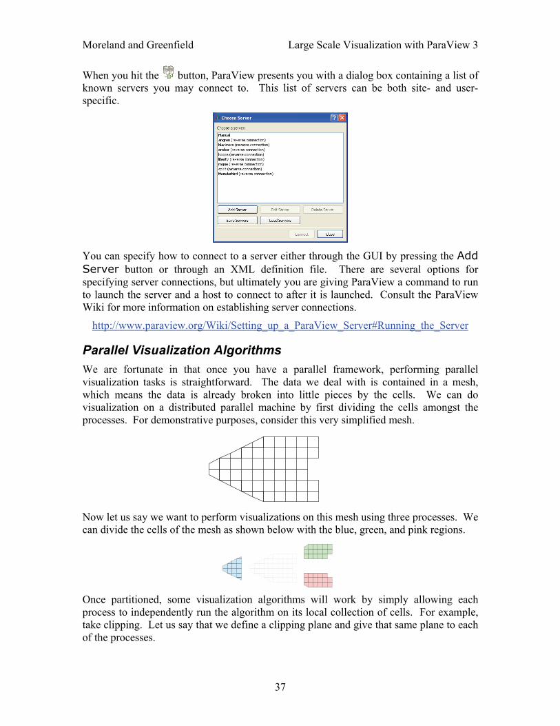
When you hit the button, ParaView presents you with a dialog box containing a list of known servers you may connect to. This list of servers can be both site- and user-specific.
You can specify how to connect to a server either through the GUI by pressing the Add Server button or through an XML definition file. There are several options for specifying server connections, but ultimately you are giving ParaView a command to run to launch the server and a host to connect to after it is launched. Consult the ParaView Wiki for more information on establishing server connections.
http://www.paraview.org/Wiki/Setting_up_a_ParaView_Server#Running_the_Server
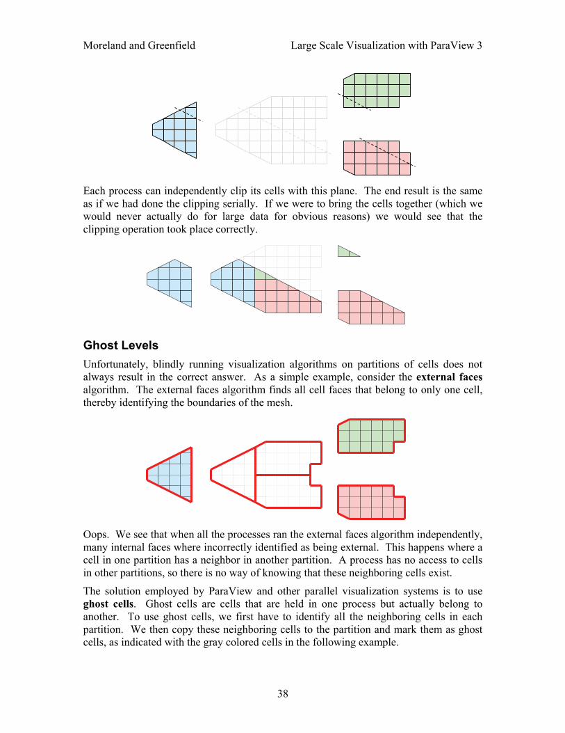
Parallel Visualization Algorithms We are fortunate in that once you have a parallel framework, performing parallel visualization tasks is straightforward. The data we deal with is contained in a mesh, which means the data is already broken into little pieces by the cells. We can do visualization on a distributed parallel machine by first dividing the cells amongst the processes. For demonstrative purposes, consider this very simplified mesh.
Now let us say we want to perform visualizations on this mesh using three processes. We can divide the cells of the mesh as shown below with the blue, green, and pink regions.
Once partitioned, some visualization algorithms will work by simply allowing each process to independently run the algorithm on its local collection of cells. For example, take clipping. Let us say that we define a clipping plane and give that same plane to each of the processes.
37
Moreland and Greenfield Large Scale Visualization with ParaView 3
Each process can independently clip its cells with this plane. The end result is the same as if we had done the clipping serially. If we were to bring the cells together (which we would never actually do for large data for obvious reasons) we would see that the clipping operation took place correctly.
Ghost Levels Unfortunately, blindly running visualization algorithms on partitions of cells does not always result in the correct answer. As a simple example, consider the external faces algorithm. The external faces algorithm finds all cell faces that belong to only one cell, thereby identifying the boundaries of the mesh.
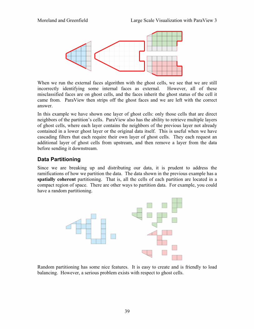
Oops. We see that when all the processes ran the external faces algorithm independently, many internal faces where incorrectly identified as being external. This happens where a cell in one partition has a neighbor in another partition. A process has no access to cells in other partitions, so there is no way of knowing that these neighboring cells exist.
The solution employed by ParaView and other parallel visualization systems is to use ghost cells. Ghost cells are cells that are held in one process but actually belong to another. To use ghost cells, we first have to identify all the neighboring cells in each partition. We then copy these neighboring cells to the partition and mark them as ghost cells, as indicated with the gray colored cells in the following example.
38
Moreland and Greenfield Large Scale Visualization with ParaView 3
When we run the external faces algorithm with the ghost cells, we see that we are still incorrectly identifying some internal faces as external. However, all of these misclassified faces are on ghost cells, and the faces inherit the ghost status of the cell it came from. ParaView then strips off the ghost faces and we are left with the correct answer.
In this example we have shown one layer of ghost cells: only those cells that are direct neighbors of the partition’s cells. ParaView also has the ability to retrieve multiple layers of ghost cells, where each layer contains the neighbors of the previous layer not already contained in a lower ghost layer or the original data itself. This is useful when we have cascading filters that each require their own layer of ghost cells. They each request an additional layer of ghost cells from upstream, and then remove a layer from the data before sending it downstream.
Data Partitioning Since we are breaking up and distributing our data, it is prudent to address the ramifications of how we partition the data. The data shown in the previous example has a spatially coherent partitioning. That is, all the cells of each partition are located in a compact region of space. There are other ways to partition data. For example, you could have a random partitioning.
Random partitioning has some nice features. It is easy to create and is friendly to load balancing. However, a serious problem exists with respect to ghost cells.
39
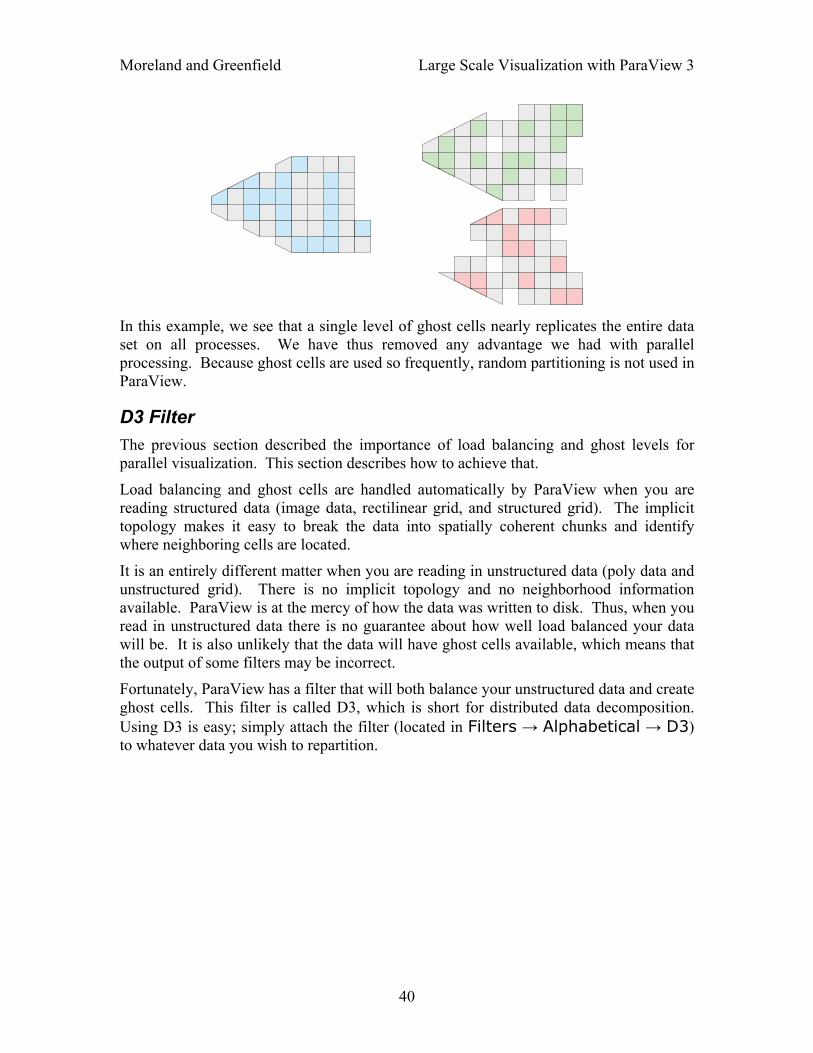
Moreland and Greenfield Large Scale Visualization with ParaView 3
In this example, we see that a single level of ghost cells nearly replicates the entire data set on all processes. We have thus removed any advantage we had with parallel processing. Because ghost cells are used so frequently, random partitioning is not used in ParaView.
D3 Filter The previous section described the importance of load balancing and ghost levels for parallel visualization. This section describes how to achieve that.
Load balancing and ghost cells are handled automatically by ParaView when you are reading structured data (image data, rectilinear grid, and structured grid). The implicit topology makes it easy to break the data into spatially coherent chunks and identify where neighboring cells are located.
It is an entirely different matter when you are reading in unstructured data (poly data and unstructured grid). There is no implicit topology and no neighborhood information available. ParaView is at the mercy of how the data was written to disk. Thus, when you read in unstructured data there is no guarantee about how well load balanced your data will be. It is also unlikely that the data will have ghost cells available, which means that the output of some filters may be incorrect.
Fortunately, ParaView has a filter that will both balance your unstructured data and create ghost cells. This filter is called D3, which is short for distributed data decomposition. Using D3 is easy; simply attach the filter (located in Filters → Alphabetical → D3) to whatever data you wish to repartition.
40

Moreland and Greenfield Large Scale Visualization with ParaView 3
The most common use case for D3 is to attach it directly to your unstructured grid reader. Regardless of how well load balance the incoming data might be, it is important to be able to retrieve ghost cell so that subsequent filters will generate the correct data. The example above shows a cutaway of the extract surface filter on an unstructured grid. On the left we see that there are many faces improperly extracted because we are missing ghost cells. On the right the problem is fixed by first using the D3 filter.
Matching Job Size to Data Size How many processors should I have in my ParaView server? This is a common question with many important ramifications. It is also an enormously difficult question. The answer depends on a wide variety of factors including what hardware each process has, how much data is being processed, what type of data is being processed, what type of visualization operations are being done, and your own patience.
Consequently, we have no hard answer. We do however have several rules of thumb.
If you are loading structured data (image data, rectilinear grid, structured grid), try to have a minimum of one processor per 20 million cells. If you can spare the processors, one processor for every 5 to 10 million cells is usually plenty.
If you are loading unstructured data (poly data, unstructured grid), try to have a minimum of one processor per 1 million cells. If you can spare the processors, one processor for every 250 to 500 thousand cells is usually plenty.
As stated before, these are just rules of thumb, not absolutes. You should always try to experiment to gage what your processor to data size should be. And, of course, there will always be times when the data you want to load will stretch the limit of the resources you have available. When this happens, you will want to make sure that you avoid data explosion and that you cull your data quickly.
Avoiding Data Explosion The pipeline model that ParaView presents is very convenient for exploratory visualization. The loose coupling between components provides a very flexible framework for building unique visualizations, and the pipeline structure allows you to tweak parameters quickly and easily.
The downside of this coupling is that it can have a larger memory footprint. Each stage of this pipeline maintains its own copy of the data. Whenever possible, ParaView performs shallow copies of the data so that different stages of the pipeline point to the
41
Moreland and Greenfield Large Scale Visualization with ParaView 3
same block of data in memory. However, any filter that creates new data or changes the values or topology of the data must allocate new memory for the result. If ParaView is filtering a very large mesh, inappropriate use of filters can quickly deplete all available memory. Therefore, when visualizing large data sets, it is important to understand the memory requirements of filters.
Please keep in mind that the following advice is intended only for when dealing with very large amounts of data and the remaining available memory is low. When you are not in danger of running out of memory, ignore all of the following advice.
When dealing with structured data, it is absolutely important to know what filters will change the data to unstructured. Unstructured data has a much higher memory footprint, per cell, than structured data because the topology must be explicitly written out. There are many filters in ParaView that will change the topology in some way, and these filters will write out the data as an unstructured grid, because that is the only data set that will handle any type of topology that is generated. The following list of filters will write out a new unstructured topology in its output that is roughly equivalent to the input. These filters should never be used with structured data and should be used with caution on unstructured data.
o Append Datasets
o Append Geometry
o Clean
o Clean to Grid
o Connectivity
o D3
o Delaunay 2D
o Extract Edges
o Linear Extrusion
o Loop Subdivision
o Reflection
o Rotational Extrusion
o Shrink
o Smooth
o Subdivide
o Tessellate
o Tetrahedralize
o Triangle Strips
o Triangulate
Technically, the Ribbon and Tube filters should fall into this list. However, as they only work on 1D cells in poly data, the input data is usually small and of little concern.
This similar set of filters also output unstructured grids, but they also tend to reduce some of this data. Be aware though that this data reduction is often smaller than the overhead of converting to unstructured data. Also note that the reduction is often not well balanced. It is possible (often likely) that a single process may not lose any cells. Thus, these filters should be used with caution on unstructured data and extreme caution on structured data.
o Clip
o Decimate
o Extract Cells by Region
o Extract Selections
o Extract Thresholds
o Quadric Clustering
42
Moreland and Greenfield Large Scale Visualization with ParaView 3
o Threshold
Similar to the items in the preceding list, Extract Subset performs data reduction on a structured data set, but also outputs a structured data set. So the warning about creating new data still applies, but you do not have to worry about converting to an unstructured grid.
This next set of filters also outputs unstructured data, but it also performs a reduction on the dimension of the data (for example 3D to 2D), which results in a much smaller output. Thus, these filters are usually safe to use with unstructured data and require only mild caution with structured data.
o Cell Centers
o Contour
o Extract CTH Parts
o Extract Surface
o Feature Edges
o Mask Points
o Outline (curvilinear)
o Slice
o Stream Tracer
These filters do not change the connectivity of the data at all. Instead, they only add field arrays to the data. All the existing data is shallow copied. These filters are usually safe to use on all data.
o Calculator
o Cell Data to Point Data
o Curvature
o Elevation
o Gradient
o Gradient (Unstructured)
o Gradient Magnitude
o Level Scalars
o Median
o Mesh Quality
o Normals Generation
o Octree Depth Limit
o Octree Depth Scalars
o Point Data to Cell Data
o Process Id Scalars
o Random Vectors
o Resample with dataset
o Surface Flow
o Surface Vectors
o Transform
o Warp (scalar)
o Warp (vector)
This final set of filters are those that either add no data to the output (all data of consequence is shallow copied) or the data they add is generally independent of the size of the input. These are almost always safe to add under any circumstances (although they may take a lot of time).
o Annotate Time
o Append Attributes
o Extract Datasets
43
Moreland and Greenfield Large Scale Visualization with ParaView 3
o Extract Group
o Glyph
o Group Datasets
o Histogram
o Integrate Variables
o Outline
o Outline Corners
o Plot Cell over Time
o Plot Field Variable over Time
o Plot Over Line
o Plot Point over Time
o Probe Location
o Probe Location over Time
o Temporal Shift Scale
There are a few special case filters that do not fit well into any of the previous classes. Some of the filters, currently Temporal Interpolator and Particle Tracer, perform calculations based on how data changes over time. Thus, these filters may need to load data for two or more instances of time, which can double or more the amount of data needed in memory. The Temporal Cache filter will also hold data for multiple instances of time.
The Programmable Filter is also a special case which is impossible to classify. Since this filter does whatever it is programmed to do, it can fall into any one of these categories.
Culling Data When dealing with large data, it is clearly best to cull out data whenever possible, and the earlier the better. Most large data starts as 3D geometry and the desired geometry is often a surface. As surfaces usually have a much smaller memory footprint than the volumes that they are derived from, it is best to convert to a surface soon. Once you do that, you can apply other filters in relative safety.
A very common visualization operation is to extract isosurfaces from a volume using the Contour filter. The Contour filter usually outputs geometry much smaller than its input. Thus, the Contour filter should be applied early if it is to be used at all. Be careful when setting up the parameters to the Contour filter because it still is possible for it to generate a lot of data. This obviously can happen if you specify many isosurface values. High frequencies such as noise around an isosurface value can also cause a large, irregular surface to form.
Another way to peer inside of a volume is to perform a Slice on it. The Slice filter will intersect a volume with a plane and allow you to see the data in the volume where the plane intersects. If you know the relative location of an interesting feature in your large data set, slicing is a good way to view it.
If you have little a-priori knowledge of your data and would like to explore the data without paying the memory and processing time for the full data set, you can use the Extract Subset filter to subsample the data. The subsampled data can be dramatically smaller than the original data and should still be well load balanced. Of
44
Moreland and Greenfield Large Scale Visualization with ParaView 3
course, be aware that you may miss small features if the subsampling steps over them and that once you find a feature you should go back and visualize it with the full data set.
There are also several features that can pull out a subset of a volume: Clip , Threshold , Extract Selection, and Extract Subset can all extract cells based on some criterion. Be aware, however, that the extracted cells are almost never well balanced; expect some processes to have no cells removed. Also, all of these filters with the exception of Extract Subset will convert structured data types to unstructured grids. Therefore, they should not be used unless the extracted cells are of at least an order of magnitude less than the source data.
When possible, replace the use of a filter that extracts 3D data with one that will extract 2D surfaces. For example, if you are interested in a plane through the data, use the Slice
filter rather than the Clip filter. If you are interested in knowing the location of a region of cells containing a particular range of values, consider using the Contour filter to generate surfaces at the ends of the range rather than extract all of the cells with the Threshold filter. Be aware that substituting filters can have an effect on downstream filters. For example, running the Histogram filter after Threshold will have an entirely different effect then running it after the roughly equivalent Contour filter.
Rendering Rendering is the process of synthesizing the images that you see based on your data. The ability to effectively interact with your data depends highly on the speed of the rendering. Thanks to advances in 3D hardware acceleration, fueled by the computer gaming market, we have the ability to render 3D quickly even on moderately priced computers. But, of course, the speed of rendering is proportional to the amount of data being rendered. As data gets bigger, the rendering process naturally gets slower.
To ensure that your visualization session remains interactive, ParaView supports two modes of rendering that are automatically flipped as necessary. In the first mode, still render, the data is rendered at the highest level of detail. This rendering mode ensures that all of the data is represented accurately. In the second mode, interactive render, speed takes precedence over accuracy. This rendering mode endeavors to provide a quick rendering rate regardless of data size.
While you are interacting with a 3D view, for example rotating, panning, or zooming with the mouse, ParaView uses an interactive render. This is because during the interaction a high frame rate is necessary to make these features usable and because each frame is immediately replaced with a new rendering while the interaction is occurring so that fine details are less important during this mode. At any time when interaction of the 3D view is not taking place, ParaView uses a still render so that the full detail of the data is available as you study it. As you drag your mouse in a 3D view to move the data, you may see an approximate rendering while you are moving the mouse, but the full detail will be presented as soon as you release the mouse button.
45
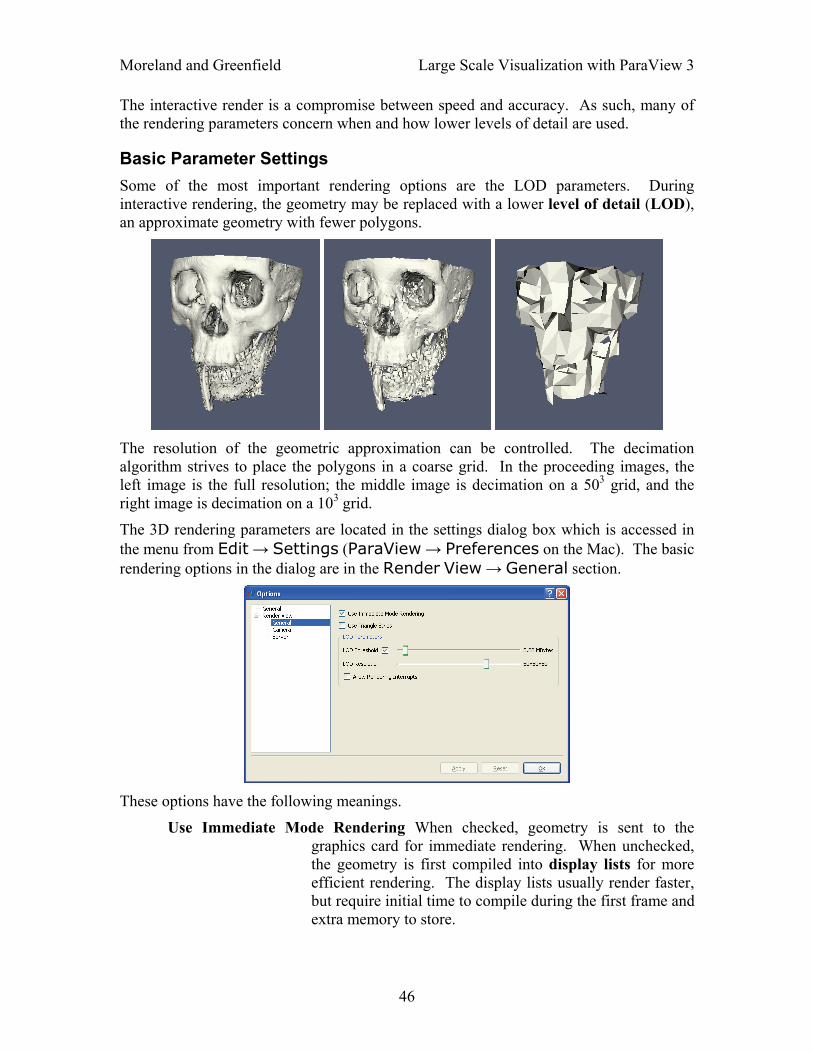
Moreland and Greenfield Large Scale Visualization with ParaView 3
The interactive render is a compromise between speed and accuracy. As such, many of the rendering parameters concern when and how lower levels of detail are used.
Basic Parameter Settings Some of the most important rendering options are the LOD parameters. During interactive rendering, the geometry may be replaced with a lower level of detail (LOD), an approximate geometry with fewer polygons.
The resolution of the geometric approximation can be controlled. The decimation algorithm strives to place the polygons in a coarse grid. In the proceeding images, the left image is the full resolution; the middle image is decimation on a 503 grid, and the right image is decimation on a 103 grid.
The 3D rendering parameters are located in the settings dialog box which is accessed in the menu from Edit → Settings (ParaView → Preferences on the Mac). The basic rendering options in the dialog are in the Render View → General section.
These options have the following meanings.
Use Immediate Mode Rendering When checked, geometry is sent to the graphics card for immediate rendering. When unchecked, the geometry is first compiled into display lists for more efficient rendering. The display lists usually render faster, but require initial time to compile during the first frame and extra memory to store.
46

Moreland and Greenfield Large Scale Visualization with ParaView 3
Use Triangle Strips When unchecked, data is rendered as defined in the poly data. When checked, the data is first converted to triangle strips. Triangle strips can be pushed to a graphics card more efficiently and can sometimes be rendered faster.
LOD Threshold Controls when to replace the geometry with a decimated version of the geometry. The checkbox turns the feature on or off. When on, the slider gives a threshold for the feature. If the geometry size is below the threshold, it is considered small enough to render. When the geometry size is above the threshold, the decimated form is used during rendering.
Allow Rendering Interrupts When checked, a still render may be interrupted by a request to perform an interactive render.
Basic Parallel Rendering When performing parallel visualization, we are careful to ensure that the data remains partitioned amongst all of the processes up to and including the rendering processes. ParaView uses a parallel rendering library called IceT. IceT uses a sort-last algorithm for parallel rendering. This parallel rendering algorithm allows each process to independently render its partition of the geometry and then composites the partial images together to form the final image.
The wonderful thing about sort-last parallel rendering is that its efficiency is completely insensitive to the amount of data being rendered. This makes it a very scalable algorithm and well suited to large data. However, the parallel rendering overhead does increase linearly with the number of pixels in the image. Consequently, some of the rendering parameters deal with the image size.
47
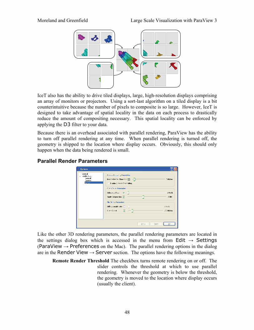
Moreland and Greenfield Large Scale Visualization with ParaView 3
IceT also has the ability to drive tiled displays, large, high-resolution displays comprising an array of monitors or projectors. Using a sort-last algorithm on a tiled display is a bit counterintuitive because the number of pixels to composite is so large. However, IceT is designed to take advantage of spatial locality in the data on each process to drastically reduce the amount of compositing necessary. This spatial locality can be enforced by applying the D3 filter to your data.
Because there is an overhead associated with parallel rendering, ParaView has the ability to turn off parallel rendering at any time. When parallel rendering is turned off, the geometry is shipped to the location where display occurs. Obviously, this should only happen when the data being rendered is small.
Parallel Render Parameters
Like the other 3D rendering parameters, the parallel rendering parameters are located in the settings dialog box which is accessed in the menu from Edit → Settings (ParaView → Preferences on the Mac). The parallel rendering options in the dialog are in the Render View → Server section. The options have the following meanings.
Remote Render Threshold The checkbox turns remote rendering on or off. The slider controls the threshold at which to use parallel rendering. Whenever the geometry is below the threshold, the geometry is moved to the location where display occurs (usually the client).
48
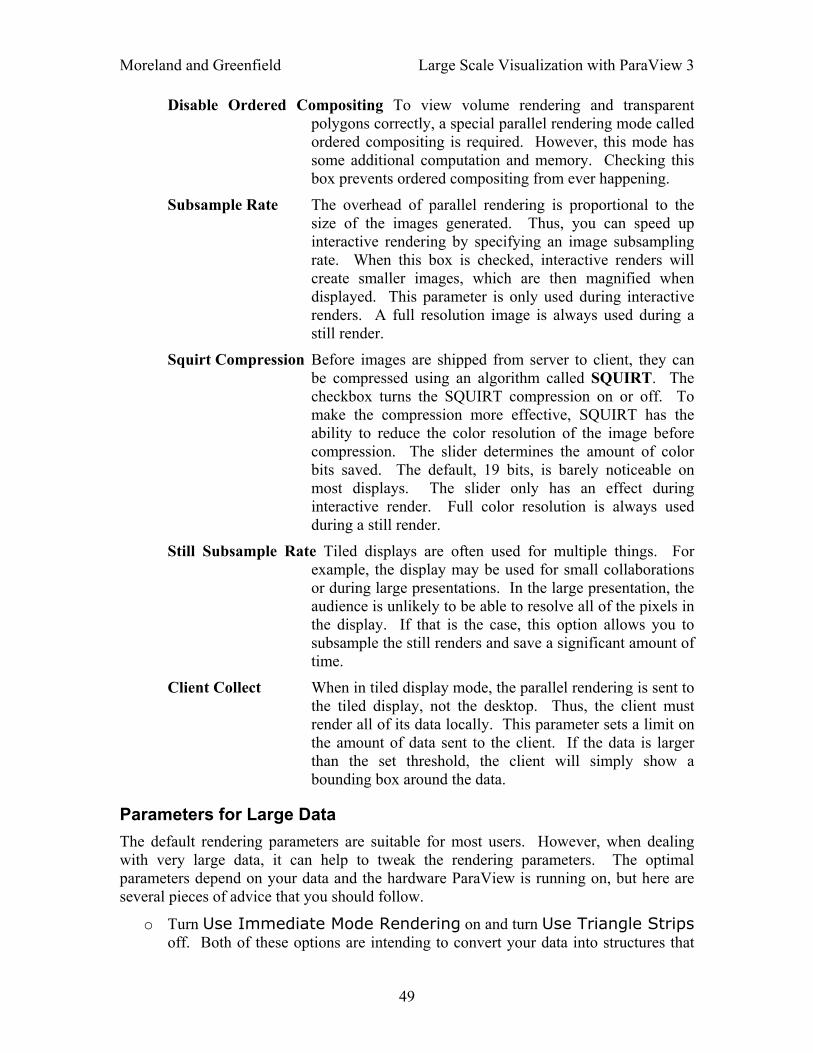
Moreland and Greenfield Large Scale Visualization with ParaView 3
Disable Ordered Compositing To view volume rendering and transparent polygons correctly, a special parallel rendering mode called ordered compositing is required. However, this mode has some additional computation and memory. Checking this box prevents ordered compositing from ever happening.
Subsample Rate The overhead of parallel rendering is proportional to the size of the images generated. Thus, you can speed up interactive rendering by specifying an image subsampling rate. When this box is checked, interactive renders will create smaller images, which are then magnified when displayed. This parameter is only used during interactive renders. A full resolution image is always used during a still render.
Squirt Compression Before images are shipped from server to client, they can be compressed using an algorithm called SQUIRT. The checkbox turns the SQUIRT compression on or off. To make the compression more effective, SQUIRT has the ability to reduce the color resolution of the image before compression. The slider determines the amount of color bits saved. The default, 19 bits, is barely noticeable on most displays. The slider only has an effect during interactive render. Full color resolution is always used during a still render.
Still Subsample Rate Tiled displays are often used for multiple things. For example, the display may be used for small collaborations or during large presentations. In the large presentation, the audience is unlikely to be able to resolve all of the pixels in the display. If that is the case, this option allows you to subsample the still renders and save a significant amount of time.
Client Collect When in tiled display mode, the parallel rendering is sent to the tiled display, not the desktop. Thus, the client must render all of its data locally. This parameter sets a limit on the amount of data sent to the client. If the data is larger than the set threshold, the client will simply show a bounding box around the data.
Parameters for Large Data The default rendering parameters are suitable for most users. However, when dealing with very large data, it can help to tweak the rendering parameters. The optimal parameters depend on your data and the hardware ParaView is running on, but here are several pieces of advice that you should follow.
o Turn Use Immediate Mode Rendering on and turn Use Triangle Strips off. Both of these options are intending to convert your data into structures that
49
Moreland and Greenfield Large Scale Visualization with ParaView 3
are more efficiently rendered. However, the processing and memory overhead are often not worth it when data is large. In fact, when the memory limits are stretched, this can actually reduce performance.
o Try turning the LOD Threshold off. The geometry decimation can take a long time with large data, and it sometimes does a poor job if your data has high curvatures or strange connectivity. If the LOD is improving your performance, try moving the LOD Resolution slider all the way to the right (10x10x10).
o Always have remote rendering on (controlled by the checkbox next to Remote Render Threshold). The remote rendering will use the power of entire server to render and ship images to the client. If remote rendering is off, geometry is shipped back to the client. When you have large data, it is always faster to ship images than to ship data.
o Turn on subsampling and adjust the Subsample Rate as needed. If image compositing is slow, if the connection between client and server has low bandwidth, or if you are rendering very large images, then a higher subsample rate can greatly improve your interactive rendering performance.
o Make sure Squirt Compression is on. It has a tremendous effect on desktop delivery performance, and the artifacts it introduces, which are only there during interactive rendering, are minimal.
50
Moreland and Greenfield Large Scale Visualization with ParaView 3
Further Reading Thank you for participating in this tutorial. Hopefully you have learned enough to get you started visualizing large data with ParaView. Here are some sources for further reading.
The ParaView Guide is a good resource to have with ParaView. An updated version for ParaView 3 is expected real soon now.
Amy Henderson Squillacote. The ParaView Guide. Kitware, Inc., 2006.
The ParaView Wiki is full of information that you can use to help you set up and use ParaView. In particular, those of you who wish to install a parallel ParaView server should consult the appropriate build and install pages.
http://www.paraview.org/Wiki/ParaView
http://www.paraview.org/Wiki/Setting_up_a_ParaView_Server
If you are interested in learning more about visualization or more specifics about the filters available in ParaView, consider picking up the following visualization textbook.
Will Schroeder, Ken Martin, and Bill Lorensen. The Visualization Toolkit. Kitware, Inc., fourth edition, 2006. ISBN 1-930934-19-X.
If you plan on customizing ParaView, the previous books and web pages have lots of information. For more information about using VTK, the underlying visualization library, and Qt, the GUI library, consider the following books have more information.
Kitware Inc. The VTK User’s Guide. Kitware, Inc., 2006.
Jasmin Blanchette and Mark Summerfield. C++ GUI Programming with Qt 4. Prentice Hall, 2006. ISBN 0-13-187249-4.
If you are interested about the design of parallel visualization and other features of the VTK pipeline, there are several technical papers available.
James Ahrens, Charles Law, Will Schroeder, Ken Martin, and Michael Papka. “A Parallel Approach for Efficiently Visualizing Extremely Large, Time-Varying Datasets.” Technical Report #LAUR-00-1620, Los Alamos National Laboratory, 2000.
James Ahrens, Kristi Brislawn, Ken Martin, Berk Geveci, C. Charles Law, and Michael Papka. “Large-Scale Data Visualization Using Parallel Data Streaming.” IEEE Computer Graphics and Applications, 21(4): 34–41, July/August 2001.
Andy Cedilnik, Berk Geveci, Kenneth Moreland, James Ahrens, and Jean Farve. “Remote Large Data Visualization in the ParaView Framework.” Eurographics Parallel Graphics and Visualization 2006, pg. 163–170, May 2006.
James P. Ahrens, Nehal Desai, Patrick S. McCormic, Ken Martin, and Jonathan Woodring. “A Modular, Extensible Visualization System Architecture for
51

Moreland and Greenfield Large Scale Visualization with ParaView 3
Culled, Prioritized Data Streaming.” Visualization and Data Analysis 2007, Proceedings of SPIE-IS&T Electronic Imaging, pg 64950I-1–12, January 2007.
John Biddiscombe, Berk Geveci, Ken Martin, Kenneth Moreland, and David Thompson. “Time Dependent Processing in a Parallel Pipeline Architecture.” IEEE Visualization 2007. October 2007.
If you are interested in the algorithms and architecture for ParaView’s parallel rendering, there are also many technical articles on this as well.
Kenneth Moreland, Brian Wylie, and Constantine Pavlakos. “Sort-Last Parallel Rendering for Viewing Extremely Large Data Sets on Tile Displays.” Proceedings of IEEE 2001 Symposium on Parallel and Large-Data Visualization and Graphics, pg. 85–92, October 2001.
Kenneth Moreland and David Thompson. “From Cluster to Wall with VTK.” Proceddings of IEEE 2003 Symposium on Parallel and Large-Data Visualization and Graphics, pg. 25–31, October 2003.
Kenneth Moreland, Lisa Avila, and Lee Ann Fisk. “Parallel Unstructured Volume Rendering in ParaView.” Visualization and Data Analysis 2007, Proceedings of SPIE-IS&T Electronic Imaging, pg. 64950F-1–12, January 2007.
Acknowledgements Thanks to Amy Squillacote, Berk Geveci, and Alan Scott for contributing material to the tutorial. And, of course, thanks to everyone at Kitware, Sandia, and CSimSoft for their hard work in making ParaView what it is today.
Sandia is a multiprogram laboratory operated by Sandia Corporation, a Lockheed Martin Company, for the United States Department of Energy’s National Nuclear Security Administration under contract DE-AC04-94AL85000.
52