Saving and habit formation: evidence from Dutch panel · 2017-08-29 · habit formation from...

Empir Econ (2010) 38:385–407DOI 10.1007/s00181-009-0272-z

ORIGINAL PAPER

Saving and habit formation: evidence from Dutch paneldata

Rob Alessie · Federica Teppa

Received: 19 March 2007 / Accepted: 18 June 2008 / Published online: 24 March 2009© The Author(s) 2009. This article is published with open access at Springerlink.com

Abstract This paper focuses on the role of habit formation in individual preferences.In this study, the model of Alessie and Lusardi (Econ Lett 55:103–108, 1997) and itsextension by Guariglia and Rossi (Oxf Econ Pap 54:1–19, 2002) are considered. Ourempirical specifications are based on their closed-form solutions, where current savingis expressed as a function of lagged saving and other regressors. In our study, we usea longitudinal data set from the Netherlands that allows us to disentangle the role ofhabit formation from unobserved heterogeneity. Contrary to most other studies usingsurvey data, we find evidence in favor of habit formation. However, the magnitudeof the habit formation coefficient is rather small. Income uncertainty seems to affectsaving behavior of Dutch households.

Keywords Habit formation · Permanent income · Precautionary savings ·Panel data

JEL Classification D91

R. Alessie (B)University of Groningen & Netspar & Tinbergen Institute, Faculty of Economics and Business,P. O. Box 800, 9700 AV Groningen, The Netherlandse-mail: [email protected]

F. TeppaDe Nederlandsche Bank & Netspar, Economics and Research Division,Postbus 98, 1000 AB Amsterdam, The Netherlandse-mail: [email protected]

123

386 R. Alessie, F. Teppa

1 Introduction

The concept of habit formation relies on the idea that one’s own past consumptionmight have an effect on the utility yielded by current consumption: for a given level ofcurrent consumption, a larger habit stock lowers utility. Habits were first introducedin the context of demand systems (see, e.g. Pollak 1970). In the literature a distinctionbetween two types of habits has been made: myopic (or naive) and rational. In the firstcase (see, e.g. Pollak 1970), consumers are not aware of the effects that their currentconsumption decisions will have on their future marginal rates of substitution betweengoods and as a consequence their behavior may be time-inconsistent. In the secondcase (Spinnewijn 1981), consumers are aware of the habit forming effect of currentconsumption.

The presence of habit formation may provide an appealing (partial) explanation toa number of anomalous empirical findings contrasting some of the permanent incomemodel’s predictions, such as the “excess sensitivity” of aggregate consumption growthrelative to current labor income growth,1 its “excess smoothness” relative to laggedlabor income growth,2 the equity premium3 puzzle, and the risk-free rate4 puzzle(Abel 1990; Campbell and Cochrane 1999). Moreover, Carroll et al. (2000) show thatif one allows for habit formation, then standard growth models can be reconciled withthe empirical evidence suggesting that high growth leads to high saving, rather thanthe other way around.

In general, mixed conclusions about the strength of habit formation arise from paststudies of time-nonseparable preferences based on aggregate consumption data. Anumber of studies using aggregate consumption data (see e.g. Dunn and Singleton1986) display very little evidence of habits. However, other studies concerning USdata (Ferson and Constantinides 1991) lead to a different conclusion.

One of the most common approaches in micro-econometric studies used to test thepresence of habit formation has been the Euler equation approach. It focuses on aspecific first-order condition implied by the optimization problem faced by a genericconsumer, allowing the estimation of preference parameters. In this strand of literature,Hotz et al. (1988) examine whether intertemporally nonseparable utility functions are

1 The permanent income model predicts that consumption changes should be orthogonal to predictable,or lagged, income changes. Yet, the correlation between consumption growth and lagged income growthseems to be one of the most robust features of aggregate data (Flavin 1981; Campbell and Deaton 1989;Runkle 1991).2 The permanent income model predicts that consumption growth should be more volatile than incomegrowth if aggregate income growth has positive serial correlation. Yet, aggregate consumption growth seemsto be much smoother than aggregate income growth (Campbell and Deaton 1989). Notice however thata number of studies based on household-level data (e.g. Runkle 1991) show a strong correlation betweenconsumption growth and lagged income growth.3 Under time-separable utility, Mehra and Prescott (1985) could not find a plausible pair of subjectivediscount rate and relative risk aversion of the representative consumer to match the mean of the annual realrate of interest and of the equity premium in a US sample over a 90-year period. That is, stocks were notsufficiently riskier than Treasury bills to explain the spread of their returns.4 Weil (1989) found that in the same sample used by Mehra and Prescott (1985), although individuals likeconsumption to be very smooth and although the risk-free rate is very low, they still save enough so thatper-capita consumption grows rapidly.

123

Saving and habit formation: evidence from Dutch panel data 387

important in characterizing microdata on life-cycle labor supply behavior among whitemale workers in the U.S. They find empirical support for the hypothesis that agents’preferences directly depend upon past leisure decisions and for the relatively simplespecification of nonseparable preferences. More recently, Meghir and Weber (1996)argue that the within marginal rate of substitution function can be used as a controlwhen evaluating results obtained using the intertemporal Euler equation. They use alarge sample of US households, drawn from twelve years of the Consumer Expendi-ture Survey to model the intertemporal and within period allocation of expenditure onfood in the home, transport, and services, and they allow for the presence of liquidityconstraints. Their findings show no empirical support for intertemporal non-separabil-ity of preferences over the three categories of consumption. Similarly, Dynan (2000)finds no evidence of habit formation at the annual frequency. Her analysis on foodconsumption data from the Panel Study on Income Dynamics indicates that habit for-mation has at most a limited impact on consumers’ behavior. This finding is robustto a number of changes in the model’s specification. However, both these studies donot control explicitly for time invariant unobserved heterogeneity across households,that may lead to a spurious relationship between future and past consumption. UsingSpanish panel data, Carrasco et al. (2005) build on the study by Meghir and Weber(1996) and show how crucial it is to account for fixed effects when testing for the pres-ence of habit formation in consumption decisions.5 If fixed effects are not taken intoaccount, they find evidence of intertemporally separable preferences.6 However thisresult is not robust once they control for time invariant unobserved heterogeneity acrosshouseholds: in this case, a significant role of habit formation is found. More recently,Malley and Molana (2006) use U.S. time series data on consumers’ expenditures anddisposable income from the U.S. National Income and Product Accounts coveringthe period 1929–2001 to estimate the path of aggregate consumption implied by thepermanent income model. They find a significant and robust role of habit formation.

An alternative approach to the Euler equation is adopted by Alessie and Lusardi(1997), who derive closed-form solutions for consumption (and saving) under theassumption of CARA within period preferences. Closed-form solutions for consump-tion and saving allow a better understanding of some of the issues concerning thosevariables, as they provide a rich specification that extends some of the previous resultsin the literature. A problem with the model of Alessie and Lusardi (1997) is that it doesnot preclude negative consumption. A detailed description of Alessie and Lusardi’smodel is provided in Sect. 2.

Guariglia and Rossi (2002) generalize Weil’s non-expected utility model (1993)by allowing for habit formation. They obtain a closed-form solution for saving as afunction of, among other things, lagged consumption. Their model can be seen as anextension of Alessie and Lusardi (1997), as in the closed form solution of Alessie andLusardi (1997) the lagged consumption variable does not appear as an explanatoryvariable. Guariglia and Rossi (2002) then derive an Euler equation of consumptionchanges, where current consumption changes depend on lagged changes and labor

5 Carrasco et al. (2005) focus on the same consumption items as Meghir and Weber (1996), namely foodat home, transport and services.6 This result is in line with both Meghir and Weber (1996) and Dynan (2000).

123


income risk.7 They estimate this Euler equation using food consumption data fromthe British Household Panel Survey for the period 1992–1997, by allowing for unob-served time invariant heterogeneity in preferences. They find that both labor incomerisk and past changes in consumption are important in determining current changesin consumption. In particular, their estimation results suggest that the lagged changesin consumption display a strong statistically significant negative effect on the currentchanges. This suggests that the utility function exhibits durability in Deaton (1992)sense, rather than habit formation. It is worthwhile saying that Guariglia and Rossi’sempirical model can also be justified by the model by Alessie and Lusardi (1997).In other words Guariglia and Rossi (2002) cannot infer empirically whether or nottheir extension of Weil’s model describes household behavior in a better way than themodel of Alessie and Lusardi (1997).

In this paper, we estimate the models of Alessie and Lusardi (1997) and Guarigliaand Rossi (2002). Our empirical models are based on their closed-form solutions,8

where saving is expressed as a function of lagged saving and other regressors. We optfor this choice because the closed form solution embodies more information about thehabit formation model than the Euler equation does, and allows for a more powerful testof the validity of the habit formation model than the alternative approach. For exam-ple, contrary to Guariglia and Rossi (2002) we are able to discriminate empiricallybetween the models of Alessie and Lusardi (1997) and Guariglia and Rossi (2002).However, we have to qualify a bit the remark about the advantages of using the closedform solution in the empirical exercise: the closed form solution approach relies moreheavily on proxy variables (e.g. we need a proxy for the expected discounted value offuture income changes).

The remainder of the paper is organized as follows. In Sect. 2, we present thetheoretical model. Section 3 describes our dataset, Sect. 4 provides the empiricalimplementation, and Sect. 5 contains the empirical results. Section 6 concludes thepaper.

2 The theoretical model for habit formation and precautionary saving

In this section we describe the theoretical model we will use for empirical tests. Westrictly refer to Alessie and Lusardi (1997) model of habit formation, in its precau-tionary saving specification.

The reference model is the one by Caballero (1990), with a Constant AbsoluteRisk Aversion (CARA) utility function and an uncertain non-capital income (incomeis assumed to be a strictly exogenous variable), following a moving-average processwith ψi representing the i th MA coefficient. Hence:

Et yτ − Et−1 yτ = ψτ−twt , τ ≥ t (1)

7 In the derivation of the Euler equation, Guariglia and Rossi (2002) assume that the rate of time preferenceequals the real interest rate.8 Alternatively, we could have used the Euler-equation approach (see e.g., Guariglia and Rossi (2002) andDynan (2000)).

123


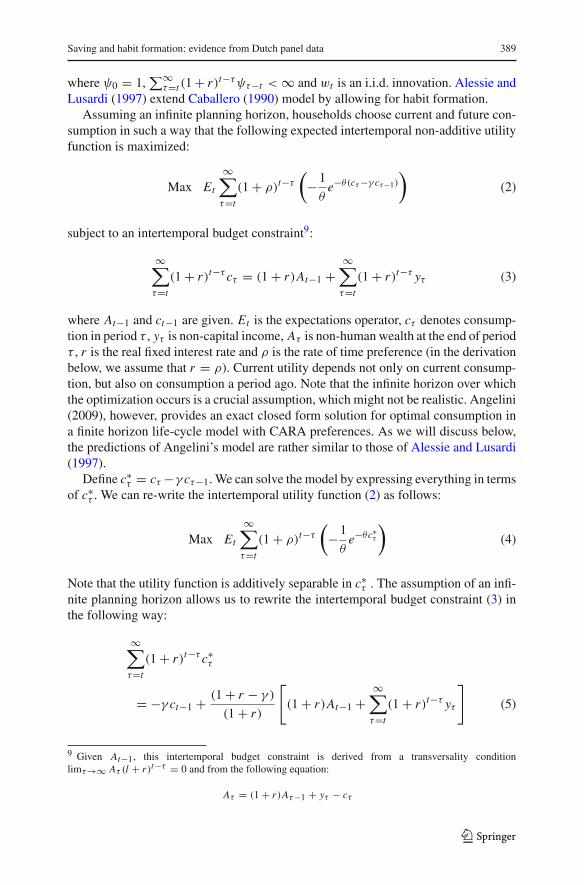
where ψ0 = 1,∑∞τ=t (1 + r)t−τψτ−t < ∞ and wt is an i.i.d. innovation. Alessie and

Lusardi (1997) extend Caballero (1990) model by allowing for habit formation.Assuming an infinite planning horizon, households choose current and future con-

sumption in such a way that the following expected intertemporal non-additive utilityfunction is maximized:

Max Et

∞∑

τ=t

(1 + ρ)t−τ(

−1

θe−θ(cτ−γ cτ−1)

)

(2)

subject to an intertemporal budget constraint9:

∞∑

τ=t

(1 + r)t−τ cτ = (1 + r)At−1 +∞∑

τ=t

(1 + r)t−τ yτ (3)

where At−1 and ct−1 are given. Et is the expectations operator, cτ denotes consump-tion in period τ , yτ is non-capital income, Aτ is non-human wealth at the end of periodτ , r is the real fixed interest rate and ρ is the rate of time preference (in the derivationbelow, we assume that r = ρ). Current utility depends not only on current consump-tion, but also on consumption a period ago. Note that the infinite horizon over whichthe optimization occurs is a crucial assumption, which might not be realistic. Angelini(2009), however, provides an exact closed form solution for optimal consumption ina finite horizon life-cycle model with CARA preferences. As we will discuss below,the predictions of Angelini’s model are rather similar to those of Alessie and Lusardi(1997).

Define c∗τ = cτ −γ cτ−1. We can solve the model by expressing everything in terms

of c∗τ . We can re-write the intertemporal utility function (2) as follows:

Max Et

∞∑

τ=t

(1 + ρ)t−τ(

−1

θe−θc∗

τ

)

(4)

Note that the utility function is additively separable in c∗τ . The assumption of an infi-

nite planning horizon allows us to rewrite the intertemporal budget constraint (3) inthe following way:

∞∑

τ=t

(1 + r)t−τ c∗τ

= −γ ct−1 + (1 + r − γ )

(1 + r)

[

(1 + r)At−1 +∞∑

τ=t

(1 + r)t−τ yτ

]

(5)

9 Given At−1, this intertemporal budget constraint is derived from a transversality conditionlimτ→∞ Aτ (l + r)t−τ = 0 and from the following equation:

Aτ = (1 + r)Aτ−1 + yτ − cτ

123


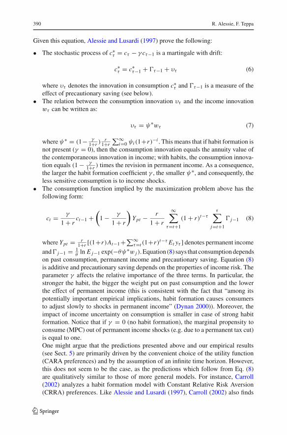
Given this equation, Alessie and Lusardi (1997) prove the following:

• The stochastic process of c∗τ = cτ − γ cτ−1 is a martingale with drift:

c∗τ = c∗

τ−1 + �τ−1 + υτ (6)

where υτ denotes the innovation in consumption c∗τ and �τ−1 is a measure of the

effect of precautionary saving (see below).• The relation between the consumption innovation υτ and the income innovationwτ can be written as:

υτ = ψ∗wτ (7)

whereψ∗ = (1− γ1+r )

r1+r

∑∞i=0 ψi (1+r)−i . This means that if habit formation is

not present (γ = 0), then the consumption innovation equals the annuity value ofthe contemporaneous innovation in income; with habits, the consumption innova-tion equals (1 − γ

1+r ) times the revision in permanent income. As a consequence,the larger the habit formation coefficient γ , the smaller ψ∗, and consequently, theless sensitive consumption is to income shocks.

• The consumption function implied by the maximization problem above has thefollowing form:

ct = γ

1 + rct−1 +

(

1 − γ

1 + r

)

Ypt − r

1 + r

∞∑

τ=t+1

(1 + r)t−ττ∑

j=t+1

� j−1 (8)

where Ypt = r1+r [(1+r)At−1 +∑∞

τ=t (1+r)t−τ Et yτ ] denotes permanent income

and� j−1 = 1θ

ln E j−1 exp(−θψ∗w j ). Equation (8) says that consumption dependson past consumption, permanent income and precautionary saving. Equation (8)is additive and precautionary saving depends on the properties of income risk. Theparameter γ affects the relative importance of the three terms. In particular, thestronger the habit, the bigger the weight put on past consumption and the lowerthe effect of permanent income (this is consistent with the fact that “among itspotentially important empirical implications, habit formation causes consumersto adjust slowly to shocks in permanent income” (Dynan 2000)). Moreover, theimpact of income uncertainty on consumption is smaller in case of strong habitformation. Notice that if γ = 0 (no habit formation), the marginal propensity toconsume (MPC) out of permanent income shocks (e.g. due to a permanent tax cut)is equal to one.One might argue that the predictions presented above and our empirical results(see Sect. 5) are primarily driven by the convenient choice of the utility function(CARA preferences) and by the assumption of an infinite time horizon. However,this does not seem to be the case, as the predictions which follow from Eq. (8)are qualitatively similar to those of more general models. For instance, Carroll(2002) analyzes a habit formation model with Constant Relative Risk Aversion(CRRA) preferences. Like Alessie and Lusardi (1997), Carroll (2002) also finds

123


that the MPC out of permanent income shocks is considerably lower than one ifhabit formation is an important phenomenon. In addition, Angelini (2009) extendsthe model of Alessie and Lusardi (1997) by considering a finite horizon. Herclosed form solution is similar to Eq. (8), but the coefficients corresponding topermanent income and lagged consumption are age specific. However, for youngand middle aged people those coefficients barely change with age. In otherwords, Eq. (8) seems to effectively describe the consumption behavior of suchindividuals.

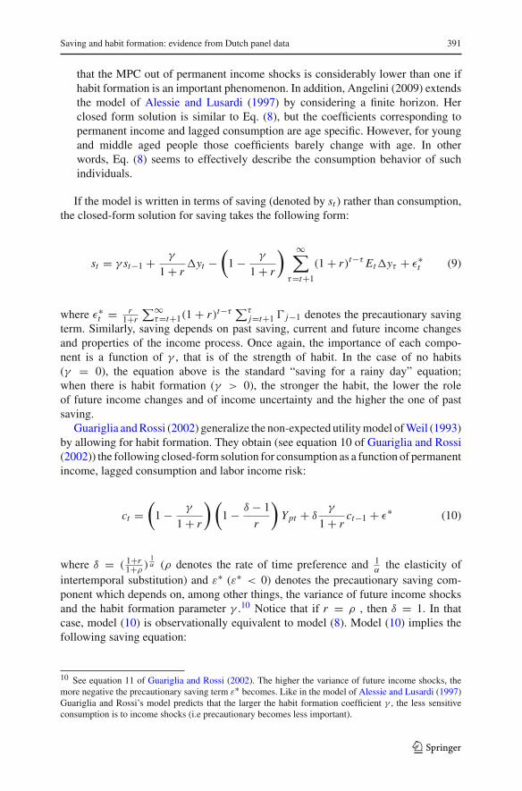
If the model is written in terms of saving (denoted by st ) rather than consumption,the closed-form solution for saving takes the following form:

st = γ st−1 + γ

1 + r�yt −

(

1 − γ

1 + r

) ∞∑

τ=t+1

(1 + r)t−τ Et�yτ + ε∗t (9)

where ε∗t = r1+r

∑∞τ=t+1(1 + r)t−τ

∑τj=t+1 � j−1 denotes the precautionary saving

term. Similarly, saving depends on past saving, current and future income changesand properties of the income process. Once again, the importance of each compo-nent is a function of γ , that is of the strength of habit. In the case of no habits(γ = 0), the equation above is the standard “saving for a rainy day” equation;when there is habit formation (γ > 0), the stronger the habit, the lower the roleof future income changes and of income uncertainty and the higher the one of pastsaving.

Guariglia and Rossi (2002) generalize the non-expected utility model of Weil (1993)by allowing for habit formation. They obtain (see equation 10 of Guariglia and Rossi(2002)) the following closed-form solution for consumption as a function of permanentincome, lagged consumption and labor income risk:

ct =(

1 − γ

1 + r

) (

1 − δ − 1

r

)

Ypt + δγ

1 + rct−1 + ε∗ (10)

where δ = ( 1+r1+ρ )

1α (ρ denotes the rate of time preference and 1

αthe elasticity of

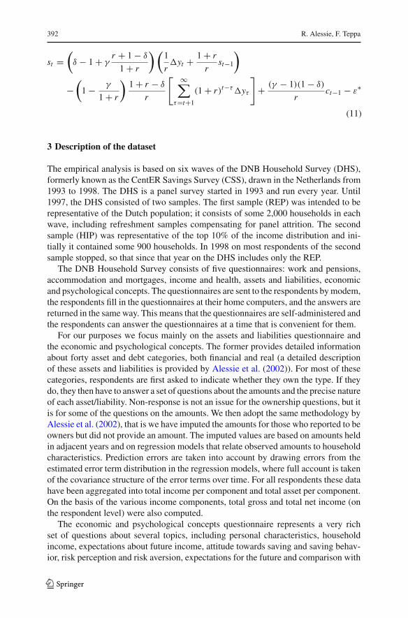
intertemporal substitution) and ε∗ (ε∗ < 0) denotes the precautionary saving com-ponent which depends on, among other things, the variance of future income shocksand the habit formation parameter γ .10 Notice that if r = ρ , then δ = 1. In thatcase, model (10) is observationally equivalent to model (8). Model (10) implies thefollowing saving equation:

10 See equation 11 of Guariglia and Rossi (2002). The higher the variance of future income shocks, themore negative the precautionary saving term ε∗ becomes. Like in the model of Alessie and Lusardi (1997)Guariglia and Rossi’s model predicts that the larger the habit formation coefficient γ , the less sensitiveconsumption is to income shocks (i.e precautionary becomes less important).

123


st =(

δ − 1 + γr + 1 − δ

1 + r

) (1

r�yt + 1 + r

rst−1

)

−(

1 − γ

1 + r

)1 + r − δ

r

[ ∞∑

τ=t+1

(1 + r)t−τ�yτ

]

+ (γ − 1)(1 − δ)

rct−1 − ε∗

(11)

3 Description of the dataset

The empirical analysis is based on six waves of the DNB Household Survey (DHS),formerly known as the CentER Savings Survey (CSS), drawn in the Netherlands from1993 to 1998. The DHS is a panel survey started in 1993 and run every year. Until1997, the DHS consisted of two samples. The first sample (REP) was intended to berepresentative of the Dutch population; it consists of some 2,000 households in eachwave, including refreshment samples compensating for panel attrition. The secondsample (HIP) was representative of the top 10% of the income distribution and ini-tially it contained some 900 households. In 1998 on most respondents of the secondsample stopped, so that since that year on the DHS includes only the REP.

The DNB Household Survey consists of five questionnaires: work and pensions,accommodation and mortgages, income and health, assets and liabilities, economicand psychological concepts. The questionnaires are sent to the respondents by modem,the respondents fill in the questionnaires at their home computers, and the answers arereturned in the same way. This means that the questionnaires are self-administered andthe respondents can answer the questionnaires at a time that is convenient for them.

For our purposes we focus mainly on the assets and liabilities questionnaire andthe economic and psychological concepts. The former provides detailed informationabout forty asset and debt categories, both financial and real (a detailed descriptionof these assets and liabilities is provided by Alessie et al. (2002)). For most of thesecategories, respondents are first asked to indicate whether they own the type. If theydo, they then have to answer a set of questions about the amounts and the precise natureof each asset/liability. Non-response is not an issue for the ownership questions, but itis for some of the questions on the amounts. We then adopt the same methodology byAlessie et al. (2002), that is we have imputed the amounts for those who reported to beowners but did not provide an amount. The imputed values are based on amounts heldin adjacent years and on regression models that relate observed amounts to householdcharacteristics. Prediction errors are taken into account by drawing errors from theestimated error term distribution in the regression models, where full account is takenof the covariance structure of the error terms over time. For all respondents these datahave been aggregated into total income per component and total asset per component.On the basis of the various income components, total gross and total net income (onthe respondent level) were also computed.

The economic and psychological concepts questionnaire represents a very richset of questions about several topics, including personal characteristics, householdincome, expectations about future income, attitude towards saving and saving behav-ior, risk perception and risk aversion, expectations for the future and comparison with

123


the current situation, planning of financial matters. For our purposes, we focus on anumber of questions related to saving behavior.

Equation (9) is the starting point of our empirical analysis. It should be stressed thatwe cannot estimate consumption equation (8) because the DHS data does not containdirect information on consumption. We now provide a description of the variablesused in the estimation procedure.

1. In the DHS, the dependent variable sit (saving by household i in year t) can bemeasured as follows. First, we use information about whether any money hasbeen put aside in the previous 12 months by an individual. Then they are askedto indicate how much money their household has put aside in the same period.In our analysis we do not use limited dependent variable estimation techniquefor reasons explained in footnote 11. It is therefore important to deal with “nomoney put aside” answers (1,907 cases out of the 6,602 cases). We have furtherinvestigated these cases by crossing them with other informative variables in thequestionnaire, in order to check for potential dissaving. In particular, we haveconsidered the following question:“Over the past 12 months, would you say the expenditures of your household werehigher than the income of the household, about equal the income of the household,or lower than the income of the household?”Second, we treat the dependent variable, sit , as a continuous variable, representedby the amount of money put aside.11 We have constructed this variable as follows.For those who have claimed to have put no money aside and whose expenditureswere about equal the income of the household, it was clear that they have notsaved and not dissaved either. We then have imputed zero as the amount of moneyput aside (1,701 cases). For those who have claimed to have put no money asideand whose expenditures were higher than the income of the household, we haveconstructed a change in liquid financial wealth as a proxy of their dissaving andimputed that negative value as the amount of money put aside (141 observations).Finally, for those who have claimed to have put no money aside and whose expen-ditures were lower than the income of the household, we have constructed a changein liquid financial wealth as a proxy of their saving and imputed that (positive)value as the amount of money put aside, in order to overcome the contradiction(65 cases). In constructing the imputed variable mentioned above, we have usedinformation about wealth. For each year, we have picked the most liquid cate-gories for assets (checking accounts, savings arrangements, linked to a Postbankaccount, deposit books, savings or deposit accounts, savings certificates) net ofthe most liquid categories of liabilities (private loans and extended lines of credit)

11 Respondents report the amount of money put aside in classes. Out of this piece of information we haveconstructed a “continuous” variable by taking the mid-points for each class. Alternatively, we could haveadopted a Limited Dependent Variable (LDV) technique (e.g. ordered probit) to obtain estimates of theparameters. However, our empirical habit formation model is clearly dynamic and allows for unobservedheterogeneity by including an individual effect. Obviously, some of the right hand side variables (apart fromlagged saving) may be correlated with the individual effect. The estimation of LDV models which allowfor both state dependence and correlated unobserved heterogeneity is notoriously difficult. Therefore, weabstain from such an approach.

123


and then taken first differences. We have deleted extreme values in order to avoidincluding outliers in our imputations.12

Obviously, we could have obtained an alternative saving measure by computingthe first differences in (liquid) wealth (�At ). We will argue in the next sectionthat using this measure may result in a spuriously negative estimate of the habitformation parameter.

2. Income change: We build a variable (“Realised income change”) from the follow-ing set of questions:A. “The total net income of your household consists of the income of all members

of the household, after deduction of taxes and premiums for social insurancepolicies, taken as the sum total over the past 12 months. Compared to aboutone year ago, did the total net income of your household increase, remainabout the same, or decrease?”

B. “By what percentage (approximately) has the total net income of your house-hold increased/decreased?”

We then transform percentages into amounts and use the latter specification in theempirical estimation.

3. Expectations on income change: Two time-horizon lenghts are considered, as weexploit the following questions:A1. “Do you think the total net income of your household will increase, remain

the same, or decrease in the next 12 months?”A2. “By what percentage do you think the total net income of your household

will increase/decrease in the next 12 months?”B1. “Do you think the total net income of your household will increase, remain

the same, or decrease in the next 5 years?”B2. “By what percentage do you think the total net income of your household

will increase/decrease in the next 5 years?”Two variables are then constructed: variable “Expected income change (next12 months)” refers to questions A1–A2, variable “Expected income change (next5 years)” refers to questions B1–B2. Both variables are in amounts.

4. Uncertainty on expected income change: Based on Das and Donkers (1999) andHochguertel (2003), we exploit seven questions related to uncertainty about futureincome. First, respondents are asked how probable it is that next year incomeincreases by more than 15%. They can answer on a seven-point scale rangingfrom “very unlikely” to “very likely”. The same type of question is asked for anincrease of between 10 and 15%, between 5 and 10%, no change, a decrease of

12 One may argue that the estimation results may be “dominated” by the imputed continuous savings datafor those who do not put money aside although it concerns a few observations. In order to investigatethis issue, we have also created an alternative measure for saving, by imputing averages of the change infinancial wealth for two classes of individuals:• individuals who do not report putting money aside and claim that their expenditures were lower than

income (average change fin. wealth = −10, 490);• individuals who do not report putting money aside and claim that their expenditures were higher than

income (average change fin. wealth = 9,873).This revised saving measure only takes 10 different values, namely −10490, 0, 1,500, 6,500, 9,873, 17,500,32,500, 57,500, 112,500, and 150,000 guilders. See Sect. 5 for a summary of the estimation results usingthis alternative saving measure.

123


between 5 and 10%, a decrease of between 10 and 15% and a decrease of morethan 15%. We follow the suggestion of Das and Donkers (1999) and constructedprobabilities for the categories of income changes in the following way:

Pj = W j∑7

k=1 Wk, j = 1, . . . , 7 (12)

where W j is the answer to question j concerning income uncertainty ( j =1, . . . , 7). Question 1 concerns income increase of more than 15%,…, question7 an income decrease of more than 15%. The variable W j takes the followingvalues: 1 (very unlikely), . . ., 7 (very likely). Given Eq. (12) it is rather easy tocompute the variance of the change income between now and next year (variable“Variance of 1-year change in future income”). In the calculation of “Variance of1-year change in future income” we take for each category of income change themidpoint (e.g. 7.5 in case of the category between 5 and 10).In a sensitivity analysis we have also considered an alternative measure of incomeuncertainty. For each of the time-horizon lenghts described above, people areasked the following question:“How certain do you feel about this income change? ”Individuals have to indicate their degree of uncertainty among four possibilities:very certain, rather certain, not very certain, not at all certain. Two categoricalvariables are then built: “... about inc. change (next 12 mths)” and “... about inc.change (next 5 years)” for 12 months expectations and for 5 years expectations,respectively. This measure of uncertainty is in line with other studies (see, e.g.Hochguertel 2003) relying on subjective information about the income process.

5. Background characteristics: We add a number of individual characteristics, suchas the number of adults and children and age classes (in dummies). In particular,the six age classes consist of age less than or equal 30 years, age between 31 and40, age between 41 and 50, age between 51 and 60, age between 61 and 70, andage more than 70. The latter class serves as reference group.

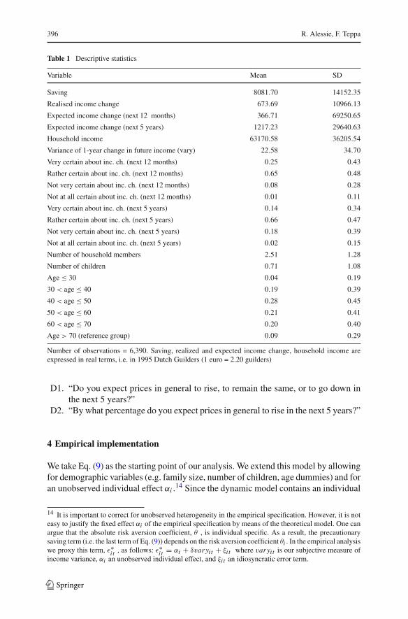
Table 1 reports summary statistics for the variables just described and used in theempirical study. In the empirical estimations, financial variables are used in real terms,as savings, financial wealth and income are deflated by means of the consumer priceindex. Deflating is also relevant for both the variable “Variance of 1-year change infuture income”and the expected income growth question, which ask about nominalgrowth. We correct for price changes by using a measure of expected inflation derivedfrom the following set of questions13:

C1. “Do you expect prices in general to rise, to remain the same, or to go down inthe next 12 months?”

C2. “By what percentage do you expect prices in general to rise in the next 12months?”

13 Note that we cannot deflate the uncertainty about expected income changes given the way this piece ofinformation is conveyed (see point 4).

123


Table 1 Descriptive statistics

Variable Mean SD

Saving 8081.70 14152.35

Realised income change 673.69 10966.13

Expected income change (next 12 months) 366.71 69250.65

Expected income change (next 5 years) 1217.23 29640.63

Household income 63170.58 36205.54

Variance of 1-year change in future income (vary) 22.58 34.70

Very certain about inc. ch. (next 12 months) 0.25 0.43

Rather certain about inc. ch. (next 12 months) 0.65 0.48

Not very certain about inc. ch. (next 12 months) 0.08 0.28

Not at all certain about inc. ch. (next 12 months) 0.01 0.11

Very certain about inc. ch. (next 5 years) 0.14 0.34

Rather certain about inc. ch. (next 5 years) 0.66 0.47

Not very certain about inc. ch. (next 5 years) 0.18 0.39

Not at all certain about inc. ch. (next 5 years) 0.02 0.15

Number of household members 2.51 1.28

Number of children 0.71 1.08

Age ≤ 30 0.04 0.19

30 < age ≤ 40 0.19 0.39

40 < age ≤ 50 0.28 0.45

50 < age ≤ 60 0.21 0.41

60 < age ≤ 70 0.20 0.40

Age > 70 (reference group) 0.09 0.29

Number of observations = 6,390. Saving, realized and expected income change, household income areexpressed in real terms, i.e. in 1995 Dutch Guilders (1 euro = 2.20 guilders)

D1. “Do you expect prices in general to rise, to remain the same, or to go down inthe next 5 years?”

D2. “By what percentage do you expect prices in general to rise in the next 5 years?”

4 Empirical implementation

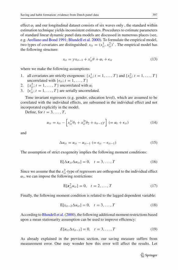
We take Eq. (9) as the starting point of our analysis. We extend this model by allowingfor demographic variables (e.g. family size, number of children, age dummies) and foran unobserved individual effect αi .14 Since the dynamic model contains an individual

14 It is important to correct for unobserved heterogeneity in the empirical specification. However, it is noteasy to justify the fixed effect αi of the empirical specification by means of the theoretical model. One canargue that the absolute risk aversion coefficient, θ , is individual specific. As a result, the precautionarysaving term (i.e. the last term of Eq. (9)) depends on the risk aversion coefficient θi . In the empirical analysiswe proxy this term, ε∗i t , as follows: ε∗i t = αi + δvaryit + ξi t where varyit is our subjective measure ofincome variance, αi an unobserved individual effect, and ξi t an idiosyncratic error term.

123


effect αi and our longitudinal dataset consists of six waves only , the standard withinestimation technique yields inconsistent estimates. Procedures to estimate parametersof standard linear dynamic panel data models are discussed in numerous places (see,e.g. Arellano and Bond 1991; Blundell et al. 2000). To formulate the empirical model,two types of covariates are distinguished: xit = (x1

i t , x2i t )

′ . The empirical model hasthe following structure:

sit = γ sit−1 + x ′i tθ + αi + εi t (13)

where we make the following assumptions:

1. all covariates are strictly exogenous: {x1i t ; t = 1, . . . , T } and {x2

i t ; t = 1, . . . , T }uncorrelated with {εi t ; t = 1, . . . , T }

2. {x2i t ; t = 1, . . . , T } uncorrelated with αi

3. {ε1i t ; t = 1, . . . , T } are serially uncorrelated.

Time invariant regressors (e.g. gender, education level), which are assumed to becorrelated with the individual effects, are subsumed in the individual effect and notincorporated explicitly in the model.

Define, for t = 3, . . . , T ,

uit = sit −[x1′

i t θ1 + x2′i t θ2 + sit−1γ

](= αi + εi t ) (14)

and

�uit = uit − uit−1 (= εi t − εi t−1) (15)

The assumption of strict exogeneity implies the following moment conditions:

E[�xi t�uit ] = 0, t = 3, . . . , T (16)

Since we assume that the x2i t -type of regressors are orthogonal to the individual effect

αi , we can impose the following restrictions:

E[x2i t uit ] = 0, t = 2, . . . , T (17)

Finally, the following moment condition is related to the lagged dependent variable:

E[sit−2�uit ] = 0, t = 3, . . . , T (18)

According to Blundell et al. (2000), the following additional moment restrictions basedupon a mean stationarity assumption can be used to improve efficiency:

E[uit�sit−1] = 0, t = 3, . . . , T (19)

As already explained in the previous section, our saving measure suffers frommeasurement error. One may wonder how this error will affect the results. Let

123


sit = s∗i t + νi t where s∗

i t and sit denote “true” and measured saving respectively(νi t is the measurement error in saving which is assumed to be I.I.D. distributed).In the presence of measurement error, the composite error term uit is equal to:uit = αi + εi t + νi t − γ νi t−1 (see Dynan 2000). In that case, the moment conditions(16) and (17) are still valid, conditions (18) and (19) however are not. Consequently,we do not use moment conditions (18) and (19) in our estimation procedure. Instead,in the main specification we impose the following moment conditions:

E[sit− j�uit ] = 0, j = 3, 4 (20)

E[uit�sit− j ] = 0, j = 2, 3 (21)

The moment conditions (20) and (21) are valid under the assumption that the mea-surement errors νi t are transitory (i.e. independent over time).15 However, those twomoment conditions are not valid if there is persistence in the measurement error. Wecarry out a Dif–Sargan test in order to check whether we can impose those momentconditions. Moreover, it can be shown that autocorrelation in the measurement errorsit also implies third order autocorrelation in �uit . We test for the presence of thirdorder autocorrelation in �uit .

In order to improve efficiency, in particular the efficiency of the habit formationcoefficient, we exploit additional information on saving behavior provided by theDHS. The following question is taken into consideration:

“How well can you manage on the total income of your household?1 very hard, 2 hard, 3 neither hard nor easy, 4 easy, 5 very easy ”.

On the basis of this information we construct a vector of instruments x3i t consisting of

three dummy variables (“neither hard or easy”, “easy” and “very easy”). Given thisinformation, we are able to exploit the following moment conditions in estimation:

E[x3i t−2�uit ] = 0 (22)

E[�x3i t−1uit ] = 0 (23)

We think that we can interpret the x3i t variables as qualitative measures of saving

behavior. In order to check this claim, we first regress sit on x3i t . It appears that the

x3i t variables predict saving (R2 = 0.14, F-statistic = 360.52). Notice that these extra

moment conditions are only valid if the measurement errors contained in the dummyvariables x3

i t are not correlated with the measurement error in our saving measure sit .We then estimate the model without using moment conditions (22) and (23) and checkthe validity of restrictions (22) and (23) by means of a Dif–Sargan test.

To summarize, for a given specification, i.e., given choices of x1i t and x2

i t , momentconditions (16), (17), (20), (21 ), (22) and (23) can be used for the so-called “systemGMM estimation”. However, one may feel uncomfortable with the mean stationarityassumptions (cf. moment conditions (21) and (23)). Therefore, we have also estimatedthe model while dropping these moment conditions. The GMM estimation techniqueallows for any type of heteroskedasticity in αi and εi t . Sargan tests for overidentifying

15 Bond et al. (2001) already proposed the method to deal with transitory measurement problem which weemploy in this paper.

123


restrictions are used to test the validity of the moment restrictions. Moreover, wealways present a difference Sargan test to check the validity of the moment conditions(21) and (23).

The assumption that the error terms εi t are serially uncorrelated seems quite strong,but it is common in this type of model. This assumption will be tested by checking forsecond order autocorrelation in the error terms in the differenced equations. To estimatethe empirical models, we use the Stata routine xtabond2 which has been developedby Roodman (2006). This program implements the so-called “system-GMM” esti-mator. Moreover, it implements the Windmeijer (2005) finite-sample correction tothe reported standard errors in the two-step estimation, without which those standarderrors tend to be severely downward biased.

5 Empirical results

Table 2 reports results for the estimation of coefficients in Equation (9) according toseveral alternative specifications. Column (1) refers to the base model defined on thefollowing specification (cf. moment conditions (16), (17), (20), (21), (22) and (23)):x1

i t includes the following variables: number of adults (in logs), ln(1+number of chil-dren), realized income change,16 both short and long run expectations about futureincome changes and the precautionary saving term, i.e. the degree of uncertainty aboutfuture income changes. x2

i t includes a full set of year and age class dummies.The base model passes some mis-specification tests. The Hansen test in column

(1) suggests that the over-identifying restrictions cannot be rejected (the value of theHansen statistic is 101.5 (degrees of freedom 95) with a p value of 0.306). The resultsof the difference Sargan test indicate that the moment conditions (17) are valid (thevalue of the Dif–Sargan statistic is 51.13 with a p value of 0.112). We also perform aDif–Sargan in order to check whether it is allowed to impose the moment conditions(22) and (23). The validity of those moment restrictions is not rejected (χ2

24 = 30.97,p value = 0.155). In comparison with the base model the parameter estimate of thehabit formation coefficient, 0.145, does not change dramatically if we do not exploitmoment conditions (22) and (23) in estimation. However, this coefficient estimate isless precise albeit significant at the 10% level (p value 0.094).17

In the empirical model it is assumed that the error term is serially uncorrelated.The second order autocorrelation test does not indicate rejection of the assumptionthat {ε1

i t ; t = 1, . . . , T } are serially uncorrelated. In Sect. 4 it is mentioned that mea-surement error in saving could cause third order serial correlation. We do not findevidence for this (see Table 2). When using the alternative saving measure computedas described in footnote 12, our estimation results barely change. Therefore, one canconclude that the estimation results are not “dominated” by the imputed continuoussavings data for those who do not put money aside.

16 In Sect. 2 we already mentioned that in the theoretical model, income is assumed to be a strictly exoge-nous variable.17 We obtain a much more precise coefficient estimate of the habit formation coefficient if we ignore thepossibility that saving is measured with error (i.e. if we use moment conditions (18) and (19) instead of(20) and (21)): γ̂ = 0.185, SD(γ̂ ) = 0.066.

123


Tabl

e2

Hab

itfo

rmat

ion

mod

el(s

ever

alal

tern

ativ

esp

ecifi

catio

ns)

Var

iabl

eB

ase

mod

elM

odel

2M

odel

3M

odel

4

Lag

ged

savi

ng0.

211*

*(0

.11)

0.22

1**

(0.0

93)

−0.4

56**

(0.1

9)0.

171*

(0.0

94)

Rea

lized

inco

me

chan

ge0.

184*

**(0

.027

)0.

180*

**(0

.019

)0.

0671

(0.1

0)0.

188*

**(0

.026

)

Exp

ecte

din

com

ech

ange

(nex

t12

mon

ths)

−0.0

009*

*(0

.000

4)−0.0

008*

*(0

.000

3)−0.0

001

(0.0

029)

−0.0

009*

*(0

.000

4)

Exp

ecte

din

com

ech

ange

(nex

t5ye

ars)

0.05

47*

(0.0

33)

0.04

06(0

.033

)0.

531*

(0.2

9)0.

0453

(0.0

31)

Var

ianc

eof

1-ye

arch

ange

infu

ture

inco

me

0.01

50**

*(0

.005

1)−0

.000

6(0

.077

)0.

0152

***

(0.0

053)

Rat

her

cert

ain

abou

tinc

.ch.

(nex

t12

mon

ths)

−0.3

11(0

.44)

Not

very

cert

ain

abou

tinc

.ch.

(nex

t12

mon

ths)

−0.1

68(0

.63)

Not

atal

lcer

tain

abou

tinc

.ch.

(nex

t12

mon

ths)

0.16

8(0

.87)

Rat

her

cert

ain

abou

tinc

.ch.

(nex

t5ye

ars)

0.13

7(0

.54)

Not

very

cert

ain

abou

tinc

.ch.

(nex

t5ye

ars)

−0.5

09(0

.70)

Not

atal

lcer

tain

abou

tinc

.ch.

(nex

t5ye

ars)

−0.9

32(1

.01)

Lag

ged

hous

ehol

din

com

e0.

0114

(0.0

13)

ln(n

o.ad

ults

)2.

885*

*(1

.23)

1.83

7(1

.23)

−1.8

98(1

6.4)

2.67

4**

(1.0

8)

ln(1

+no

.of

child

ren)

0.55

1(1

.09)

−0.4

32(1

.01)

−2.0

82(9

.17)

0.46

9(1

.06)

Num

ber

ofob

serv

atio

ns41

9448

5426

0941

94

pva

lue

Han

sen

test

0.30

60.

038

0.69

20.

177

pva

lue

diff

eren

ceSa

rgan

test

0.11

20.

243

0.62

30.

111

pva

lue

AR

1te

st0.

001

0.00

00.

470

0.00

0

pva

lue

AR

2te

st0.

839

0.32

50.

171

0.99

5

pva

lue

AR

3te

st0.

132

0.15

9.

0.17

4

All

mod

els

incl

ude

both

year

and

age

clas

sdu

mm

ies

(cf.

Tabl

e1)

.The

follo

win

gm

omen

tco

nditi

ons

are

impo

sed:

(1)

E[�

x1 it�

u it]

=0;

x1 it=

ln(n

o.ad

ults

),ln

(1+

no.

child

ren)

,rea

lized

and

exp

inc.

ch.(

12m

onth

s,5

year

s),p

rec

sav

mea

sure

(s);

(2)E

[�x2 it�

u it]

=0,

E[x

2 itu i

t]=

0:x2 it

=Y

eara

ndag

ecl

ass

dum

mie

s;(3

)E[s i

t−3�

u it]

=0

and

E[u i

t�s i

t−2]=

0,pl

usm

omen

t(22

)an

d(2

3)(s

eem

ain

text

)M

odel

2m

odel

with

alte

rnat

ive

prox

yva

riab

les

for

prec

autio

nary

savi

ng,M

odel

3sa

ving

=ch

ange

infin

anci

alw

ealth

,Mod

el4

mod

elof

Gua

rigl

iaan

dR

ossi

(200

2)St

anda

rder

rors

inpa

rent

hese

s:**

*p<

0.01

;**

p<

0.05

;*p<

0.1

123


Moreover, we follow the suggestion of Nickell and Nicolitsas (1999) and check therequirement of instrument relevance by means of two F tests.18 We carry out two firststage regressions. In the first one we perform a random effects regression of�sit−1 on�xit (see Eq. 13), sit−3 and x3

i t−2 (see equation (22)). Then we test the joint hypothe-sis that the coefficients corresponding to “remaining” instruments sit−3 and x3

i t−2 areequal to zero. The second F test checks whether �sit−2, �sit−3 and �x3

i t−1 explainsit−1 (after having corrected for x2

i t ). We find the following F values (p values): 13.93(0.000) for the first F test and 50.14 (0.001) for the second one.19 Stock and Watson(2003) have formulated a rule of thumb which says that the F value should exceed10 in order to circumvent the problem of weak instruments. In our analysis, both firststage regressions satisfy this requirement.

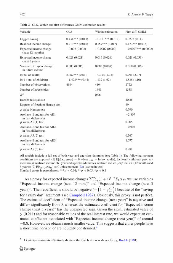
In the base model, the estimated habit formation parameter γ is equal to 0.211 anddiffers significantly from 0 at the 5 percent level (t value 1.96). It is interesting tocompare these results with those presented in Table 3, reporting OLS, Within Groupsand First Difference GMM estimations. In all regressions, year and age class dummiesare included but not reported in the table for space reasons. If we do not allow forunobserved heterogeneity, the OLS estimate of the habit formation coefficient getsconsiderably larger: 0.434 (t value 32.2). This result is not surprising, as it is wellknown that if unobserved heterogeneity is neglected, then the OLS estimate is upwardbiased (see Blundell et al. 2000). This result indicates that the unobserved hetero-geneity may partly explain the positive raw correlation between saving and laggedsaving. When performing the Within Groups estimation, the coefficient correspond-ing to lagged saving is negative (−0.12) and significant (t value −6.48). This result isalso in line with Blundell et al. (2000), who report that if T (=the number of waves inthe panel) is small, the within estimate of the lagged dependent variable is downwardbiased. Notice however that in Blundell et al. (2000) no other regressors are consid-ered when assessing the direction of the bias. The final column of Table 3 reportsresults from the First Difference GMM estimation in which the possibility that savingis measured with error is taken into account.20 One would expect the first-differenceGMM estimate to fall between the OLS and the within-group estimate. This is indeedthe case: the habit formation coefficient is slightly positive (0.027) and insignificant(t value 0.26). Notice that this estimate falls rather close to the within-group estimate.

Another feature to emphasize is that the estimate of the habit formation coefficientγ is close to the one for the realized income changes parameter (the estimated γ cor-responding to lagged saving is equal to 0.211 whereas the coefficient correspondingto “realized income change” γ

1+r is 0.184). This is in line with the theoretical model:in Eq. (9) the lagged saving coefficient should be rather close to the one of “realisedincome change”.

18 We have to carry out two F tests because we estimate the parameters of the habit formation model bymeans of system-GMM which involves both level and first-difference moments.19 The additional instruments stemming from the question “How well can you manage on the total incomeof your household? ” enter significantly into the second first stage regression: the F-statistic (p value) isequal to 10.32 (0.000). However, those dummies are not jointly significant in the other first stage regression.20 Table 3 also reports the moment conditions used in estimation.

123


Table 3 OLS, Within and first differences GMM estimation results

Variable OLS Within estimation First diff. GMM

Lagged saving 0.434*** (0.013) −0.121*** (0.019) 0.0273 (0.11)

Realized income change 0.213*** (0.016) 0.157*** (0.017) 0.173*** (0.018)

Expected income change −0.002 (0.002) −0.0009 (0.002) −0.0007*** (0.0002)(next 12 months)

Expected income change 0.023 (0.021) 0.015 (0.026) 0.021 (0.033)(next 5 years)

Variance of 1-year change 0.003 (0.006) 0.003 (0.008) 0.010 (0.006)in future income

ln(no. of adults) 3.082*** (0.69) −0.324 (2.72) 0.791 (2.07)

ln(1 + no. of children) −1.478*** (0.44) 1.139 (1.62) 1.535 (1.10)

Number of observations 4194 4194 2722

Number of households 1449 1338

R2 0.06

Hansen test statistic 40.85

Degrees of freedom Hansen test 49

p value Hansen test 0.790

Arellano–Bond test for AR1 −2.807in first differences

p value AR(1) test 0.005

Arellano–Bond test for AR2 −0.902in first differences


Arellano–Bond test for AR3 1.077in first differences


All models include a full set of both year and age class dummies (see Table 1). The following momentconditions are imposed: (1) E[�xi t�uit ] = 0 where xi t = ln(no. adults), ln(1+no. children), prec savmeasure(s), realized income ch., year and age class dummies, realized inc. ch., exp inc. ch. (12 months and5 years); (2) E[sit−3�uit ] = 0 , plus moment (22) (see main text)Standard errors in parentheses: ***p < 0.01; **p < 0.05; *p < 0.1

As a proxy for expected income changes∑∞τ=t (1 + r)t−τ Et�yτ we use variables

“Expected income change (next 12 mths)” and “Expected income change (next 5

years)”. Their coefficients should be negative (−(

1 − γ1+r

)) because of the “saving

for a rainy day” argument (see Campbell 1987). Obviously, this proxy is not perfect.The estimated coefficient of “Expected income change (next year)” is negative anddiffers significantly from 0, whereas the estimated coefficient for “Expected incomechange (next 5 years)” has the unexpected sign. Given the small estimated value ofγ (0.211) and for reasonable values of the real interest rate, we would expect an esti-mated coefficient associated with “Expected income change (next year)” of around−0.8. However, we obtain a much smaller value. This suggests that either people havea short time horizon or are liquidity constrained.21

21 Liquidity constraints effectively shortens the time horizon as shown by e.g. Runkle (1991).

123


In the base model, we capture the precautionary saving motive by including thevariable “Variance of 1-year change in future income” defined in the data section. Wefind that the precautionary saving motive plays a significant positive role in savingbehavior. This finding is in line with the evidence provided by Guariglia and Rossi(2002). Given the small estimated value of γ (0.211) this result turns out to coin-cide with the predictions of the theoretical model: the weaker the habit formation thestronger the precautionary saving motive.

As for the demographic variables, we observe (see Table 2) that saving behavioris affected significantly by both the number of adults and household composition.The age class dummies are jointly insignificant.22 This result might be explained bythe fact that we included a full set of year dummies. In a sensitivity analysis, wealso extend the model by including labor market status dummies. Contrary to bothMeghir and Weber (1996) and Carrasco et al. (2005), we do not find any significanteffect of labor market variables.

To summarize, our evidence indicates that habit formation is a relevant phenom-enon. In that respect, our results differ from those of Guariglia and Rossi (2002),as they get a negative, strongly significant estimate for γ . As already mentioned inthe introduction, they interpret this negative sign as an indicator of “durability” inDeaton (1992) sense. Dynan (2000) estimates a similar Euler equation as Guarigliaand Rossi (2002) but she considers food consumption instead of total consumption.Dynan (2000) also obtains a negative estimate for γ , albeit insignificant. Since foodis a clearly non-durable good, her negative estimate cannot be explained by means ofa durability argument.

However, another interpretation for the findings of Guariglia and Rossi (2002) andDynan (2000) can be provided. Their estimates come from the Euler equation forconsumption rather than from a closed form solution similar to our Eq. (13). Thedata at their disposal refers to consumption expenditures (rather than savings) whichare presumably measured with considerable error. Such measurement errors might beresponsible for a strong spurious negative correlation between differences in current(�cit ) and past consumption levels (�cit−1). As one can infer from the analysis byDynan (2000), the OLS estimate of the habit formation parameter γ is severely biaseddownward: even if the true habit formation coefficient is greater than zero, the esti-mated coefficient might be lower than zero and no standard attenuation bias towardszero occurs.23 Guariglia and Rossi (2002) indeed performed a formal test of instrumentvalidity, as in Nickell and Nicolitsas (1999). They regressed the first-differences of thelagged dependent variable and their uncertainty term on all the exogenous variables

22 The p value of the Wald test of the hypothesis that all five age coefficients are jointly equal to zerois 0.67.23 Dynan (2000) shows that the error term of the Euler equation has the following form: ζi t + νi t − (1 +γ )νi t−1 +γ νi t−2, where zetait and νiτ , τ = t, t −1, t −2 denote the forecast error and the measurementerrors in consumption respectively. If one ignores other RHS variables (this is a simplifying assumption)and if one assumes that the measurement error is IID distributed, one can easily show that the OLS estimate

of the habit formation parameter γ , converges to: plim γ̂O L S = γ − (1 + 2γ ) σ2ν

var(�cit−1). If the mea-

surement errors are sizable, it is well conceivable that the OLS estimate of the habit formation coefficientconverges to a negative number.

123


in their Eq. (13) plus the remaining instruments, using a GLS random-effects method.They then tested for the joint significance of the later instruments, using a Wald test.In both cases, they obtained p values equal to 0.00, indicating that the instrumentsgenerally have sufficient explanatory power. Moreover, they also used a system-GMMestimator, proposed by Blundell and Bond (1998), which combines the standard set ofequations in first differences with suitably lagged first-differences as instruments. Thelatter instruments are generally highly informative and allow to overcome the weakinstrument bias. In other words, the empirical results of Guariglia and Rossi (2002)should be taken seriously.

In order to better understand the role of precautionary saving, we perform a sensitiv-ity analysis by using an alternative measure of income uncertainty. Instead of the mea-sure employed by Das and Donkers (1999), we only consider the information relatedto how (un)certain respondents are about income changes next year and 5 years ahead(see also Hochguertel 2003). The results are summarized in Table 2, column “model 2”.In this case we do not find any evidence for precautionary saving. The other parameterestimates are not much affected by the choice of the precautionary saving measure.

It is worth noting that our definition of saving is based on information about moneyput aside and wealth. An alternative definition would be computing first differences inwealth. In the latter specification, our empirical model would take the following form:

�At = γ�At−1 + x ′i tθ + αi + εi t (24)

Obviously, there exists a strong negative correlation between �At and �At−1because At is measured with considerable error. If we estimate Eq. (24) by means ofOLS we get a negative estimate for γ . Even by applying GMM (see Table 2, column“Model 3”), we obtain a significant negative estimate of γ : −0.46 (standard error0.19). Given the fact that At is measured with error, we have employed the followingmoment conditions instead of Eqs. (20) and (21):

E[�Ait−4�uit ] = 0 (25)

E[uit�(�Ait−3)] = 0 (26)

This procedure would imply a loss of one year of observations, the number of obser-vations dropping from 4,194 to 2,609. More importantly, the problem with the systemGMM estimation is that we do not have good instruments for�Ait−1 (and�(�Ait−1))at our disposal, because this saving measure is extremely noisy.24 As a consequence,we have decided not to build (and work with) the saving measure with informationabout differences in wealth.

Finally, we consider Guariglia and Rossi (2002) extension of the model of Alessieand Lusardi (1997) (cf. Eq. 11). This model implies that we should extend the empiricalmodel (13) by adding lagged consumption to the right hand side:

24 As we did for the main specification (cf. Table 2), we perform two F tests to investigate whether weare able to predict the endogenous RHS variables�Ait−1 and�(�Ait−1). Unfortunately, we end up withlow F values and high p values. For the �Ait−1 regression the F value (p value) is equal to 2.50 (0.041)and for the �(�Ait−1) regression equal to 1.76 (0.135).

123


sit = ζ1sit−1 + x ′i tθ + ζ2cit−1 + αi + εi t (27)

Since we do not observe consumption directly, we rewrite Eq. (27) as follows:

sit = (ζ1 − ζ2)sit−1 + x ′i tθ + ζ2Yit−1 + αi + εi t (28)

where Yit−1 = total household income in year t − 1. In the estimation of Eq. (2) weassume that Yit−1 is a strictly exogenous variable but we allow for a possible cor-relation between this variable and the individual effect. It appears that the estimatedcoefficient ζ2 is rather small and not significantly different from 0 (see Table 2, col-umn “Model 4”). This result can be explained by ρ is approximately equal to r (ifthey are exactly equal then ζ2 = 0). In other words, we do not reject the hypothesisthat Guariglia and Rossi (2002) model and the one of Alessie and Lusardi (1997) areobservationally equivalent. This result should be interpreted with care. If r is close toρ, one needs a lot of observations in order to get a significant estimate for ζ2. Ourdataset is presumably too small in order to get such a precise estimate.

6 Conclusions

This paper focuses on the role of habit formation in individual preferences. In thisstudy, the model of Alessie and Lusardi (1997) and its extension by Guariglia andRossi (2002) are considered. Our empirical specifications are based on their closed-form solutions, where saving is expressed as a function of lagged saving and otherregressors. In our study, we use a longitudinal data set from the Netherlands thatallows us to disentangle the role of habit formation from unobserved heterogeneity.Contrary to other studies using survey data (using the Euler equation for consump-tion, both Dynan (2000) and Guariglia and Rossi (2002) find negative estimates of thehabit formation coefficient), we find evidence in favor of habit formation. However,the magnitude of the habit formation coefficient is rather small. Income uncertaintyseems also to affect saving behavior of Dutch households.

We should note that the habit formation model is not fully accepted by the data.We find evidence in favor of a short planning horizon and liquidity constraints. Moretheoretical research seems to be needed in order to investigate the joint impact ofliquidity constraints and habit formation.

Finally, up to this point we have not looked at preference interdependence (Maurerand Meier 2008), which might (partially) explain the significance of the habit forma-tion coefficient we have found. This should be on the agenda for future research.

Acknowledgments We thank Arie Kapteyn, Jan van Ours, Mario Padula, Arthur van Soest and seminarparticipants at the University of Lausanne for their helpful comments. We are very grateful to two anony-mous referees for their useful suggestions. Any remaining errors are our responsibility. In this paper, useis made of data of the DNB Household Survey (formerly known as CentER Savings Survey); we thankCentERdata at Tilburg University for supplying them.

Open Access This article is distributed under the terms of the Creative Commons Attribution Noncom-mercial License which permits any noncommercial use, distribution, and reproduction in any medium,provided the original author(s) and source are credited.

123


References

Abel A (1990) Asset prices under habit formation and catching up with the Jones. Am Econ Rev 40:38–42Alessie R, Hochguertel S, van Soest A (2002) Household portfolios in the Netherlands. In: Guiso L,

Haliassos M, Jappelli T (eds) Household portfolios. University Press, Cambridge pp 341–388Alessie R, Lusardi A (1997) Consumption, saving and habit formation. Econ Lett 55:103–108Angelini V (2009) Consumption and habit formation when time horizon is finite. Econ Lett (forthcoming)Arellano M, Bond S (1991) Some tests of specification for panel data: Monte Carlo evidence and an appli-

cation to employment equations. Rev Econ Stud 58:277–297Blundell R, Bond S (1998) Initial conditions and moment restrictions in dynamic panel data models.

J Econometrics 87:115–143Blundell R, Bond S, Windmeijer F (2000) Estimation in dynamic panel data models: improving on the

performance of the standard GMM estimators. In: Baltagi B (ed) Nonstationary panels, panel coin-tegration, and dynamic panels. Advances in econometrics, vol 15. JAI Press, Amsterdam

Bond S, Hoeffler A, Temple J (2001) GMM estimation of empirical growth models. CEPR discussion paper3048

Caballero R (1990) Consumption puzzles and precautionary savings. J Monet Econ 25:113–136Campbell J (1987) Does saving anticipate declining labor income? An alternative test of the permanent

income hypothesis. Econometrica 55:1249–1273Campbell J, Cochrane J (1999) By force of habit: a consumption-based explanation of aggregate stock

market behaviour. J Polit Econ 107:205–251Campbell J, Deaton A (1989) Why is consumption so smooth?. Rev Econ Stud 56:357–374Carrasco R, Labeaga J, Lopez-salido J (2005) Consumption and habits: evidence from panel data. Econ J

115:144–165Carroll C (2002) Risky habits and the marginal propensity to consume out of permanent income. Computing

in economics and finance, vol 42. Society for Computational EconomicsCarroll C, Overland J, Weil D (2000) Saving and growth with habit formation. Am Econ Rev 90:341–355Das M, Donkers B (1999) How certain are Dutch households about future income? An empirical analysis.

Rev Income Wealth 45:325–338Deaton A (1992) Understanding consumption. Clarendon Press, OxfordDunn K, Singleton K (1986) Modeling the term structure of interest rates under non-separable utility and

durability of goods. J Financ Econ 17:27–55Dynan K (2000) Habit formation in consumer preferences: evidence from panel data. Am Econ Rev 90:

391–406Ferson W, Constantinides G (1991) Habit persistence and durability in aggregate consumption: empirical

tests. J Financ Econ 29:199–240Flavin M (1981) The adjustment of consumption to changing expectations about future income. J Polit

Econ 89:974–1009Guariglia A, Rossi M (2002) Consumption, habit formation and precautionary saving: evidence from the

British Household Panel Survey. Oxf Econ Pap 54:1–19Hochguertel S (2003) Precautionary motives and portfolio decisions. J Appl Econ 18:61–77Hotz J, Kydland F, Sedlacek G (1988) Intertemporal preferences and labor supply. Econometrica 56:

335–360Malley J, Molana H (2006) Further evidence from aggregate data on the life-cycle-permanent-income

model. Empir Econ 31:1025–1041Maurer J, Meier A (2008) Smooth it like the ‘Joneses’? Estimating peer-group effects in intertemporal

consumption choice. Econ J 118:454–476Meghir C, Weber G (1996) Intertemporal nonseparability or borrowing restrictions? A disaggregate analysis

using a U.S. consumption panel. Econometrica 64:1151–1181Mehra R, Prescott E (1985) The equity premium: a puzzle. J Monet Econ 15:145–161Nickell S, Nicolitsas D (1999) How does financial pressure affect firms? Eur Econ Rev 43:1435–1456Pollak R (1970) Habit formation and dynamic demand function. J Polit Econ 78:745–763Roodman D (2006) How to do xtabond2: an introduction to “difference” and “system” GMM in Stata.

Center for Global Development Working Paper 103Runkle D (1991) Liquidity constraints and the permanent income hypothesis: evidence from panel data.

J Monet Econ 27:73–98Spinnewijn F (1981) Rational habit formation. Eur Econ Rev 15:91–109

123


Stock J, Watson M (2003) Introduction to econometrics. Addison-Wesley, BostonWeil P (1989) The equity premium puzzle and the risk-free rate puzzle. J Monet Econ 24:401–421Weil P (1993) Precautionary savings and the permanent income hypothesis. Rev Econ Stud 60:367–381Windmeijer F (2005) A finite sample correction for the variance of linear efficient two-step GMM estima-

tors. J Econom 126:25–51

123

Saving and habit formation: evidence from Dutch panel · 2017-08-29 · habit formation from...

Documents

Transcript of Saving and habit formation: evidence from Dutch panel · 2017-08-29 · habit formation from...