Satyen Kale (Yahoo! Research)

Joint work withElad Hazan (IBM Almaden) and Manfred Warmuth (UCSC)

x1

y1x2

y2 xT

yT

Input: pairs of unit vectors in Rn: (x1, y1), (x2, y2), …, (xT, yT)

Assumption: yt = Rxt + noise, where R is an unknown rotation matrix

Problem: find “best-fit” rotation matrix for the data, i.e.arg minR t kRxt – ytk2

kRxt – ytk2 = kRxtk2 + kytk2 – 2(yt xt>) ² R

= 2 - 2(yt xt>) ² R.

arg minR t kRxt – ytk2 = arg maxR t yt xt> ² R

Computing arg maxR M² R: “Wahba’s problem” Can be solved using SVD of M

A ² B = Tr(A> B) = ij AijBij

Linear in R

x1

y1x2

y2 xT

yT

R1 x1

Choose rot matrix R1

Predict R1x1

L1(R1) = kR1x1 – y1k2

Choose rot matrix R2

Predict R2x2

L2(R2) = kR2x2– y2k2

Choose rot matrix RT

Predict RTxT

LT(RT) = kRTxT – yTk2

R2x2RTxT

Goal: Minimize regret:Regret = t Lt(Rt) – minR t Lt(R)

Open problem from COLT 2008 [Smith, Warmuth]

Rot matrix ´ orthogonal matrix of determinant 1 Set of rot matrices, SO(n):

Non-convex: so online convex optimization techniques like gradient descent, exponentiated gradient, etc. don’t apply directly

Lie group with Lie algebra = set of all skew-symmetricmatrices

Lie group gives universal representation for all Lie groups via a conformal embedding

[Arora, NIPS ’09] using Lie group/Lie algebra structure

Based on matrix exponentiated gradient: matrix exp maps Lie algebra to Lie group

Deterministic algorithm

(T) lower bound on any such deterministic algorithm, so randomization is crucial

Assume for convenience that n is even. Bad example: xt = e1, yt = -Rtxt. Lt(Rt) = kRtxt - ytk2 = k2ytk2 = 4. So total loss = 4T.

Since n is even, both I, -I are rot matrices, andt Lt(I) + Lt(-I) = t 2kytk2 + 2kxtk2 = 4T.

Hence, minR t Lt(R) · 2T. So, Regret ¸ 2T.

Adversary can compute Rt

since alg is deterministic

Randomized algorithm with expected regret O(pnL), where L = minR t Lt(R)

Lower bound on regret of any online learning algorithm for choosing rot matrices of (pnT)

Using Hannan/Kalai-Vempala’s Follow-The-Perturbed-Leader technique based on linearity of loss function

Sample noise matrix N with i.i.d entriesdistributed uniformly in [-1/, 1/]

In round t, use Rt = arg minR 1

t-1Li(R) - N ² R.

Thm [KV’05]: Regret · O(n5/4pT).

Using SVD solution to Wahba’s problem

In round t, use Rt = arg minR 1

t-1Li(R) - N ² R.

Sample n numbers 1,2, …,n i.i.d. from the exponential distribution of density exp(-)

Sample 2 orthogonal matrices U, V from theuniform Haar measure

Set N = UV>, where = diag(1,2, …,n).

In round t, use Rt = arg minR 1

t-1Li(R) - N ² R.

Sample n numbers 1,2, …,n i.i.d. from the exponential distribution of density exp(-)

Sample 2 orthogonal matrices U, V from theuniform Haar measure

Set N = UV>, where = diag(1,2, …,n).E.g. using QR-decomposition of matrix with i.i.d. standard Gaussian entries

In round t, use Rt = arg minR 1

t-1Li(R) - N ² R.

Sample n numbers 1,2, …,n i.i.d. from the exponential distribution of density exp(-)

Sample 2 orthogonal matrices U, V from theuniform Haar measure

Set N = UV>, where = diag(1,2, …,n).

Effectively, we choose N w.p. / exp(-kNk*), where kNk*= trace norm, i.e. sum of singular values of N

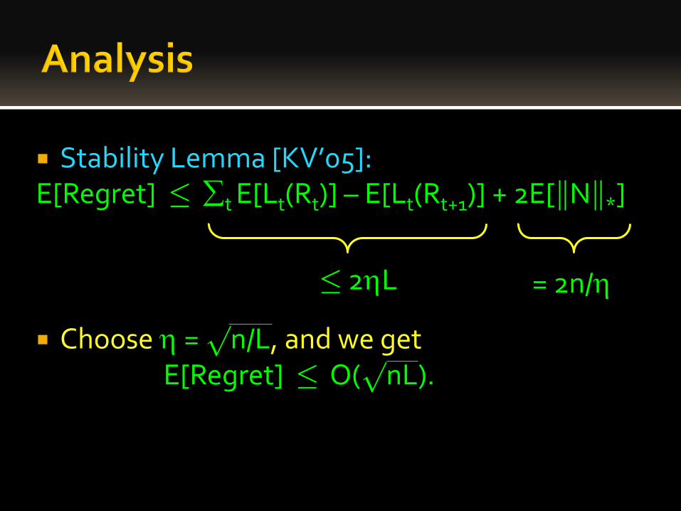
Stability Lemma [KV’05]:E[Regret] · t E[Lt(Rt)] – E[Lt(Rt+1)] + 2E[kNk*]

Choose = pn/L, and we getE[Regret] · O(pnL).

· 2L = 2n/

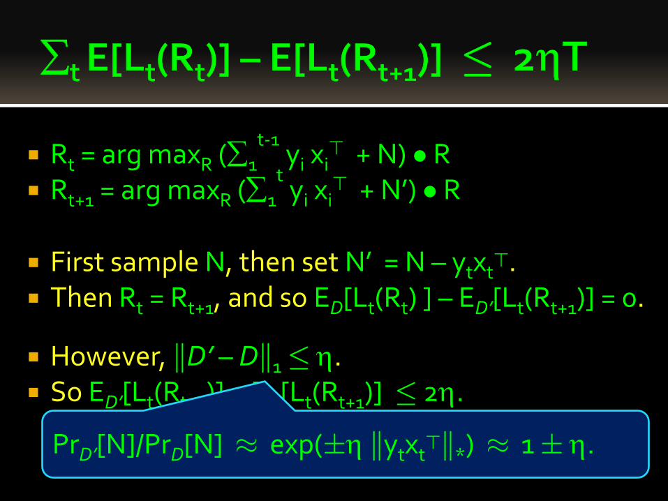
Rt = arg maxR (1

t-1yi xi

> + N) ² R Rt+1 = arg maxR (1

tyi xi

> + N’) ² R

Re-randomization doesn’t change expected regret

Rt = arg maxR (1

t-1yi xi

> + N) ² R Rt+1 = arg maxR (1

tyi xi

> + N’) ² R

First sample N, then set N’ = N – ytxt>.

Then Rt = Rt+1, and so ED[Lt(Rt) ] – ED’[Lt(Rt+1)] = 0.

D = dist of N, D’ = dist of N’

Rt = arg maxR (1

t-1yi xi

> + N) ² R Rt+1 = arg maxR (1

tyi xi

> + N’) ² R

First sample N, then set N’ = N – ytxt>.

Then Rt = Rt+1, and so ED[Lt(Rt) ] – ED’[Lt(Rt+1)] = 0.

However, kD’ – Dk1· . So ED’[Lt(Rt+1)] – ED[Lt(Rt+1)] · 2.

Rt = arg maxR (1

t-1yi xi

> + N) ² R Rt+1 = arg maxR (1

tyi xi

> + N’) ² R

First sample N, then set N’ = N – ytxt>.

Then Rt = Rt+1, and so ED[Lt(Rt) ] – ED’[Lt(Rt+1)] = 0.

However, kD’ – Dk1· . So ED’[Lt(Rt+1)] – ED[Lt(Rt+1)] · 2.

PrD’[N]/PrD[N] ¼ exp(§ kytxt>k*) ¼ 1 § .

E[kNk*] = E[i i]= i E[i]= n/.

Because i is drawn from the exponential distribution of density exp(-)

Bad example: xt = et mod n, yt = §xt w.p. ½ each

Opt rot matrix R*= diag(sgn(X1),…, sgn(Xn))

Xi = sum of § signs over all t s.t. (t mod n) = i.

* ignoring det(R*) = 1 issue

*

Bad example: xt = et mod n, yt = §xt w.p. ½ each

Opt rot matrix R*= diag(sgn(X1),…, sgn(Xn)) Expected total loss =

2T – 2i E[|Xi| ] ¸ 2T - n¢ (pT/n) = 2T - (pnT)

But for any Rt, E[Lt(Rt)] = 2 – 2E[(ytxt> ) ² Rt] = 2,

and hence total expected loss of alg = 2T.

So, E[Regret] ¸(pnT).* ignoring det(R*) = 1 issue

*

Optimal algorithm for online learning of rotations with regret O(pnL)

Based on FSPL

Open questions: Other applications for FSPL? Matrix Hedge?

Faster algorithms for SDPs? More details in Manfred’s open problem talk.

Any other example of natural problems where FPLis the only known technique that works?

Thank you!