SaTScan 9.4 Tutorial v1 · The data required for this tutorial can be found on the ... linked...
34
Transcript of SaTScan 9.4 Tutorial v1 · The data required for this tutorial can be found on the ... linked...
[email protected] SaTScan (v9.4) Tutorial # 1 Page 1

[email protected] SaTScan (v9.4) Tutorial # 1 Page 2
1. Introduction This is a step-by-step tutorial for the SaTScan™ software. SaTScan is a free software that analyzes spatial, temporal and space-time data using the spatial, temporal, or space-time scan statistics. It is designed to detect spatial or space-time disease clusters, and to determine if they are statistically significant. The software may also be used for similar problems in other fields such as archeology, criminology, demography, ecology, geography or zoology. A wide list of published application areas can be found in the SaTScan bibliography: http://www.satscan.org/references.html This tutorial is meant to serve as a quick start guide. It is intended for self-learning, but it can also be used in a classroom setting. We recommend using it as a complement to the SaTScan User Guide and to the various scientific publications describing the statistical methods. The only pre-requisite knowledge is a basic understanding of statistics and epidemiology. In this first SaTScan tutorial, we will use the purely spatial scan statistic to analyze the geographical distribution of breast cancer incidence in New York State, USA, in order to determine if there are any geographical clusters of breast cancer incidence. That is, we will determine if there are any geographical areas with more breast cancer cases than would be expected if the risk of breast cancer was evenly distributed across the state. The tutorial is written for SaTScan version 9.4 for Windows. The software tabs for subsequent versions may be slightly different than the screen shots shown in this tutorial, but they will be almost the same and there should not be a problem using the tutorial for subsequent versions. You can also use this tutorial if you use SaTScan for Linux or the Mac, except that some of the file handling steps will have to be adapted to those operating systems.
2. New York State Breast Cancer Incidence Data The data for this tutorial consists of female breast cancer incidence in New York State, for the years 2005 to 2009. The data comes from the New York State Cancer Registry, which is a part of the New York State Department of Health. It can be downloaded from the https://health.data.ny.gov/d/cw3n-fkji?category=Health&view_name=Cancer-Mapping-Data-2005-2009 website. In addition to the downloadable data, an interactive map of the data can be viewed on the NYSDOH web site. Geographical Resolution: The data are provided at the level of the census block group. Block groups are relatively homogeneous statistical units and are the smallest unit for which

[email protected] SaTScan (v9.4) Tutorial # 1 Page 3
sample-based data are tabulated by the United States Census Bureau’s American Community Survey (United States Census Bureau, 2014). In order to protect patient confidentiality, a block group needs to have a minimum of six tumors diagnosed among males and females separately. Block groups not meeting this threshold were merged with neighboring block groups. This resulted in a reduction in the number of block groups. Expected Counts: The expected counts were calculated using the indirect standardization method, adjusted for 5-year age groups up to 85+, using the 2010 census counts for New York State. In exchange for such fine geographic detail, other aspects of the data had to be omitted to ensure patient confidentiality. Accordingly, there is no information on the age, race, ethnicity, or any other demographic characteristics of the cases. Socio-economic Status: Along with New York State Cancer data, two separate files containing socioeconomic status (SES) data fields and block group crosswalk are also provided. Each of these files contains a common field, DOHREGION, which can be used for linking the cancer data with these files for further analysis. The SES file includes block group level information by sex and race, ethnicity, average household size, number of occupied and vacant housing units, number of persons above and below the poverty line, median household income, and number of persons with and without a high school education. The population counts included in this file are from the 2010 United States Census and the socioeconomic data is from the 2006-2010 American Community Survey. More information about the New York State Cancer Registry and breast cancer can be found at the http://www.health.ny.gov/statistics/cancer/registry/ and http://www.health.ny.gov/diseases/cancer/breast/ websites, respectively. Links to Original Data Sources:
Data Source Links
Cancer Data
https://health.data.ny.gov/d/cw3n-fkji?category=Health&view_name=Cancer-Mapping-Data-2005-2009
Population Data http://www2.census.gov/census_2010/04-Summary_File_1/
SES Data http://www.census.gov/acs/www/about_the_survey/american_community_survey_and_2010_census/
Link to the Data Set for this Tutorial: The data required for this tutorial can be found on the SatScan website, at http://www.satscan.org/datasets.html. The name of the file is ‘NYSCancer_Region.dbf’. Please download this file to your computer before you proceed to the next step.

[email protected] SaTScan (v9.4) Tutorial # 1 Page 4
Data Directories: SaTScan Input Files: InputFiles directory (NYSDOH Cancer Data). Data is available in txt, csv, kmz, shp and MapInfo formats in the Data directory SaTScan Output Files: OuputFiles directory Data Dictionary: InputFiles directory (Data_Dictionary_SatScan_Training.xls) Socio-demographic Data: InputFiles directory Geographical Data: InputFiles directory File required for tutorial: \sample_data\InputFiles\NYSCancer_Region.dbf
3. SaTScan Software Download and Installation To download the free SaTScan software, please go to www.satscan.org. Select “download”, and follow the instructions. In order to obtain the download password, you need to register, providing your name, email address, affiliation and country. The SaTScan software is able to depict detected clusters on Google Earth. For this feature to work, you need to install Google Earth on your computer. To download, go to http://www.google.com/earth/index.html, and follow the instructions. This is an optional step, and you can run SaTScan perfectly well without Google Earth.
4. Launching the SaTScan Software Launch the SaTScan software by using one of the following three methods. Your set-up may vary slightly on your compter.
As the next step, select “Create New Session” from the Start Window.

[email protected] SaTScan (v9.4) Tutorial # 1 Page 5
You should now see the input data tab, and you are ready to specify the anaylis you want to run. The SaTScan software has three main tabs for specifying the input data, analysis parameters and output formats respectively. We will go over each in turn. Each of the three main tabs also have a set of advanced tabs to define less used software options.
5. Input Data Tab

[email protected] SaTScan (v9.4) Tutorial # 1 Page 6
The first of the three main tabs is used to specify the input data. For a Poisson model, which we will be using, three input files are required: for the breast cancer incident cases, for the background population at risk and for the geographical information. The three files are linked through a location ID, which represents the name or code for some geographical entety such as a state, province, county, postal code area, census tract or dwelling. In the New York State data, the locations used are different Department of Health Regions (DOHREGION), with each one represented by a set of twelve integers. 5.1 Input Tab: Case File (*.cas)
If the Case File is in the SaTScan input file format (see User Guide), it is enough to specfy its name in the Case File text box. In our case, we do not have the breast cancer cases in such a format, so we will instead use the SaTScan Import Wizard.
The SaTScan import wizard can read several common file formats including *.csv, *.xlsx, *.xls, *.dbf, *.txt and *.shp. We are using a *.dbf file.
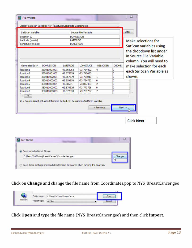
Once the import file has been selected, you must assign columns to each of the required SaTScan variables. For the case file, we first need to specify the column for the location ID, which in our case is DOHREGION. Click on the word “unassigned” that is to the right of the Location ID variable name, and then select DOHREGION. The next step is to repeat the same procedure for the number of cases. Since we are interested in breast cancer, we select OBREAST. The O in OBREAST stands for the Observed number of breast cancer cases. After finishing this tutorial, you can reapeat the analysis for a different cancer site such as bladder, bone or brain cancer. As a third step, assign YEAR as the date/time. For a purely spatial analysis, this step is optional.

[email protected] SaTScan (v9.4) Tutorial # 1 Page 7

[email protected] SaTScan (v9.4) Tutorial # 1 Page 8
After assigning all the variables, click on next. You are now asked to specify the file name and the directory in which you want to save the case file. You do not have to, but if you want to, you can change the name of the case input file, to something that is easier to remember. For this tutorial, we suggest that you do not change the directory, but do change the file name to NYS_BreastCancer.cas. This file is in the SaTScan case file format, with the extention *.cas. It is automatically assigned as the case file for the current analysis.
You can change the name of the case input file to something that is easier to remember, but it’s not necessary.

[email protected] SaTScan (v9.4) Tutorial # 1 Page 9
5.2 Population Data Once you are done with the case file, repeat the same process using the population data to create the population file. For population, you want to select the EBREAST variable, which is the expected number of breast cancer cases, adjusted for age. Population Data (*.pop):

[email protected] SaTScan (v9.4) Tutorial # 1 Page 10

[email protected] SaTScan (v9.4) Tutorial # 1 Page 11
The numbers in the population file can be either expected counts, like we have, or raw population numbers. If we had the latter, SaTScan could automatically do the age adjustment. This is done by providing SaTScan with case and population numbers stratified by age, and assigning the age variable as covariate 1 in both the case and population files. Since our expected counts are already adjusted for age, we do not have to worry about that. Instead, just click next to save the population file.
Click on Change and change the file name from Population.pop to NYS_BreastCancer.pop
Click Open and type the file name (NYS_BreastCancer.pop) and then click import.

[email protected] SaTScan (v9.4) Tutorial # 1 Page 12
5.3 Geographical Data We cannot do a spatial analysis without information about the spatial location of the cancer cases and the population. Using the same location IDs as for the cases and the population, we have to specify the geographical coordinates for each location ID. That is done using the coordinates file. Coordinates File (*.geo):
[email protected] SaTScan (v9.4) Tutorial # 1 Page 13
Click on Change and change the file name from Coordinates.pop to NYS_BreastCancer.geo
Click Open and type the file name (NYS_BreastCancer.geo) and then click import.
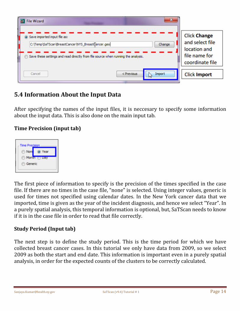
[email protected] SaTScan (v9.4) Tutorial # 1 Page 14
5.4 Information About the Input Data After specifying the names of the input files, it is neccesary to specify some information about the input data. This is also done on the main input tab. Time Precision (input tab)
The first piece of information to specify is the precision of the times specified in the case file. If there are no times in the case file, “none” is selected. Using integer values, generic is used for times not specified using calendar dates. In the New York cancer data that we imported, time is given as the year of the incident diagnosis, and hence we select “Year”. In a purely spatial analysis, this temporal information is optional, but, SaTScan needs to know if it is in the case file in order to read that file correctly. Study Period (Input tab) The next step is to define the study period. This is the time period for which we have collected breast cancer cases. In this tutorial we only have data from 2009, so we select 2009 as both the start and end date. This information is important even in a purely spatial analysis, in order for the expected counts of the clusters to be correctly calculated.

[email protected] SaTScan (v9.4) Tutorial # 1 Page 15
Coordinates (Input tab) In SaTScan, the geographical locations can either be specified as latitude and longitude, or, as Cartesian coordinates, which is the regular x,y-coordinate system taught in high school. For the New York cancer data, we have latitude and longitude coordinates. It is important to make the correct selection, since otherwise, the intended circles will not be circles. Note that, when latitude/longitude is used, SaTScan draws perfect circles on the surface of the earth, and no map projection is used.

[email protected] SaTScan (v9.4) Tutorial # 1 Page 16
5.5 Final Check of Input Tab You should now be done with the input tab, but before moving on to the next tab, it is a good idea to double check all the entries to make sure they are right. To do so, you can compare your input tab with the one below.

[email protected] SaTScan (v9.4) Tutorial # 1 Page 17
6. SaTScan Analysis Parameter Settings After providing SaTScan with the data needed to run an analysis, the next step is to tell SaTScan the type of analysis to perfrom. This is done on the Analysis Tab. Analysis Tab:
The first choice is to decide whether to do the analysis using a purely spatial, a purely temporal or a space-time scan statistic. We are not intrested in time, so we will do a purely spatial analysis.

[email protected] SaTScan (v9.4) Tutorial # 1 Page 18
Next, it is necessary to choose the probability model. We have count data, where there is a background population from which the cases arise, and where under the null hypothesis, the cases of breast cancer are independent of each other. For such data, it is suitable to use the Poisson probability model. Scan statistics are typically used to detect clusters of cases; that is, areas with a larger number of cases than would be expected by chance. This indicates areas where there may be a higher risk for the disease. Sometimes it is also of interest to look for areas with fewer cases than expected, where the risk of the disease is lower. In our case, let’s say that we are interested in areas of either high and low risk. We then select to scan for areas with high or low rates. The last option on the Analysis Tab is for Time Aggregation, but that is only relevant for purely temporal and space-time analyses. Since we are doing a purely spatial analaysis, this option is greyed out, and we simply ignore it. If we wanted to, we could now be done with the Analysis Tab and move on to the Output Tab, but we will instead go to the advanced tabs. This is reached by clicking on “Advanced” in the bottom right corner of the Analysis Tab. See the blue box below.

[email protected] SaTScan (v9.4) Tutorial # 1 Page 19
The first of the six advanced analysis tabs is called ‘Spatial Windows’, which is the one we want. The default in SaTScan is to look for clusters covering up to half the population at risk, or to be more precise, half of the total expected counts. In New York State, that can be a very large area, containing almost the whole state except New York City. To avoid the detection of such large clusters, one can set a smaller maximum on the cluster size. We will pick a maximum of 25% of the population at risk, and this is specified on the top of the ‘Spatial Windows’ tab.
Note: It is inappropriate to try different values of this maximum, running multiple SaTScan analyses. Instead, pick the largest number that you could concievably be interested in, and SaTScan will look for any cluster of that size or smaller, adjusting for the multiple testing. While we are on the advanced analaysis tabs, please go to the fourth one, which is called ‘Inference’. One important parameter there is the number of Monte Carlo replications. This should be at least 999 when running an actual analysis, although it can be set to 0 or 9 for a trial run. A larger number is always better on statistical grounds, as it will increase the statistical power of the analysis. Above 999, the increase in power is very marginal. The drawback of a larger number is that the analysis takes a longer time to run. A good rule of thumb is to use 999 for large data sets that are computer intensive to run, while using 9,999 or 99,999 for smaller data sets that are quick to run. Since we have a fairly large data set, and we want this tutorial to work on both slow and fast computers, we will pick 999. Feel free to experiment with other numbers as well. As a side note, the reason that the number of Monte Carlo replications always end 999 is that the random data sets plus the one real data set is a multiple of one thousand. This ensures that the Monte carlo based p-values have a finite number of decimals, such as 0.021

[email protected] SaTScan (v9.4) Tutorial # 1 Page 20
or 0.001, and that there are no p-values with an infinite number of decimals, such as 0.021729560302171…..
Once all the advanced parameter setting have been specified, click on ‘Close’ in the bottom right corner. If you click on ‘Set Default’, SaTScan will erase your choosen setting and return them to the default values.
7. Specifying SaTScan Output Options SaTScan gives several options to view and save the results of the scan statistic analysis. You will need to make these selections before you execute the SaTScan session. Click on the Output tab to view and select one or more options.

[email protected] SaTScan (v9.4) Tutorial # 1 Page 21
Output Tab:
There are three sections on the main output tab for text, geographical and column output format.
Click on the icon to modify/select the location of SaTScan output file. The file will be saved as a text file and will have several important sections including a summary of the data, locaction IDs of each location included in each cluster, coordinates and radius of each cluster, population, number of cases, number of expected cases, relative risk and p-value for each cluster detected.

[email protected] SaTScan (v9.4) Tutorial # 1 Page 22
SaTScan will typically find multiple overlapping clusters, some of which are almost identical to each other. In SaTScan there are options to report a different number of these overlapping clusters based on different criteria. For this tutorial, select ‘No Geographical Overlap’, which is the most restrictive choice. With this option, a secondary cluster will only be reported if it does not overlap with a more likely and previously reported cluster.

[email protected] SaTScan (v9.4) Tutorial # 1 Page 23
For the purpose of this tutorial, make selections as shown in screen below.
After you have made all the selections on the output tabs, you are ready to run a SaTScan analysis.

[email protected] SaTScan (v9.4) Tutorial # 1 Page 24
8. Running SaTScan Once all the SaTScan parameters have been selected on the various tabs, it is time to run the program. This can be done in either of two ways. From the menu, first select ‘Session’ and then ‘Execute’.
From Menu: Session > Execute Alternatively, and much faster, just click on the button with the green triangle.
Once the SaTScan analysis is running, you will see a window that shows the progress being made. There is nothing in this window that you need to write down or memorize. After the analysis is done, this window will show the text-based results file. You will be able to scroll through this window to see all the results, as well as the parameter settings you used. These are the same results that are saved in the file that you specified in section 7.

[email protected] SaTScan (v9.4) Tutorial # 1 Page 25
Sometimes SaTScan produces warnings or errors. The most common errors are problems with the input files, such as a location ID that is present in the case file but missing in the geographical coordinates file. In this tutorial, you should not get any warnings or errors if you have done everything accordining to the tutorial instructions.

[email protected] SaTScan (v9.4) Tutorial # 1 Page 26
9. Reading and Intepreting the Results The SaTScan software provides the output result in various formats, some of which are optional. The main text-based results file will automatically open once the calculations are complete:
The first thing to do is to check for any warnings or errors. These are designed to help the user find any data problems that may exist in the input files as well as unintended parameter settings. At the end of the main results file, there is a list of the parameter settings used for the analysis. For example, it states how many Monte Carlo replications were used. In this way, you can always go back and check the parameters you used for a particular analysis. At the very end, there is also information about when the SaTScan program was run, and how long it took to run it.

[email protected] SaTScan (v9.4) Tutorial # 1 Page 27
The list of parameter settings also includes the names of the optional results files that you requested, if any. These optional files contain the results in column and row format, for easy incorporation and further analysis using GIS and other software products.
[email protected] SaTScan (v9.4) Tutorial # 1 Page 29
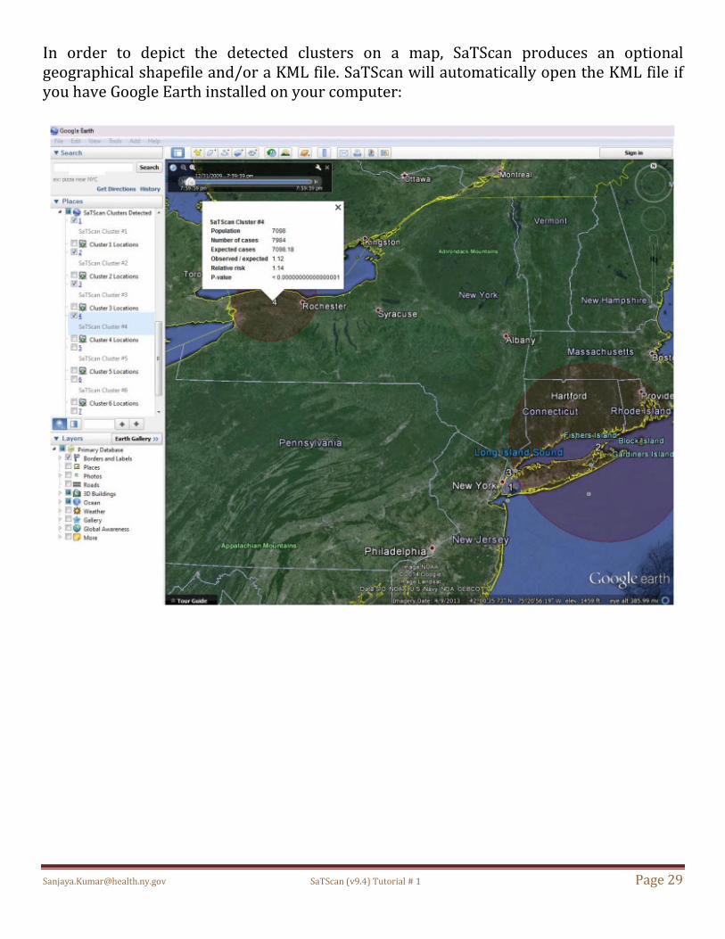
In order to depict the detected clusters on a map, SaTScan produces an optional geographical shapefile and/or a KML file. SaTScan will automatically open the KML file if you have Google Earth installed on your computer:
[email protected] SaTScan (v9.4) Tutorial # 1 Page 30
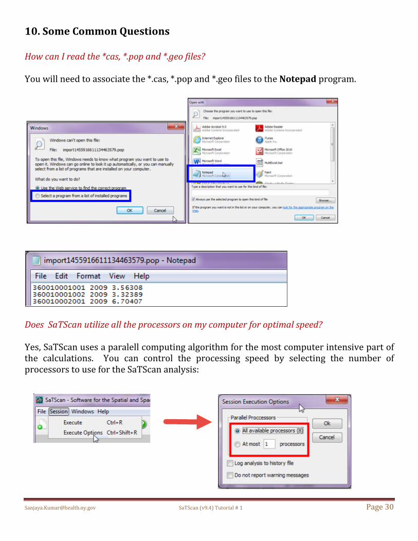
10. Some Common Questions How can I read the *cas, *.pop and *.geo files? You will need to associate the *.cas, *.pop and *.geo files to the Notepad program.
Does SaTScan utilize all the processors on my computer for optimal speed? Yes, SaTScan uses a paralell computing algorithm for the most computer intensive part of the calculations. You can control the processing speed by selecting the number of processors to use for the SaTScan analysis:

[email protected] SaTScan (v9.4) Tutorial # 1 Page 31
How can I save my parameter settings? To save time when you run the same program next time, you can save the current SaTScan session with all its parameter settings, by clicking on “File” and then “Save Session” or “Save Session As”:
How can I open a saved session? When you start SaTScan, you will be asked if you want to open an already saved session.
Alternatively, you can select “File” followed by “Open Session File” or “Reopen Session File”. Can SaTScan create kml and shp output files if my input files are in a Cartesian coordinate system? No, SaTScan must have latitude and longitude coordinates in the input file in order to create shp and kml files.

[email protected] SaTScan (v9.4) Tutorial # 1 Page 32
Can SaTScan test for non-circular shaped clusters? Yes, if the coordinate system is Cartesian, it is possible to use ellipses instead of circles. This is an advanced option on the Windows Tab.
11. References and Further Reading This is the first in a series of SaTScan tutorials. Subsequent tutorials cover space-time scan statistics; different probability models and different types of diseases. We also strongly recommend using the SaTScan User Guide. The User Guide is automatically downloaded together with the software, and can be found as a pdf file in the SaTScan directory. It can also be downloaded directly from the SaTScan web site: http://www.satscan.org/techdoc.html. For scientific publications describing the Poisson based purely spatial scan statistic, we recommend:
General Statistical Theory, Poisson Probability Model Kulldorff M. A spatial scan statistic. Communications in Statistics: Theory and Methods, 1997; 26:1481-1496. [online] Application to Breast Cancer Data with Covariate Adjustments Kulldorff M, Feuer EJ, Miller BA, Freedman LS. Breast cancer in northeastern United States: A geographical analysis. American Journal of Epidemiology, 146:161-170, 1997. [online] Sheehan TJ, DeChello LM, Kulldorff M, Gregorio DI, Gershman S, Mroszczyk M. The geographic distribution of breast cancer incidence in Massachusetts 1988-1997, adjusted for covariates. International Journal of Health Geographics, 2004, 3:17. [online] Additional references of both a methodological and applied nature can be found in the SaTScan User Guide: http://www.satscan.org/techdoc.html.

[email protected] SaTScan (v9.4) Tutorial # 1 Page 33
Please contact the authors with any comments, questions or suggestions: Thomas Talbot; New York State Department of Health [email protected] Sanjaya Kumar; New York State Department of Health [email protected] Martin Kulldorff; Harvard Medical School [email protected]

[email protected] SaTScan (v9.4) Tutorial # 1 Page 34
NOTES --------------------------------------------------------------------------------------------------------------------------------------------------------------------------------------------------------------------------------------------------------------------------------------------------------------------------------------------------------------------------------------------------------------------------------------------------------------------------------------------------------------------------------------------------------------------------------------------------------------------------------------------------------------------------------------------------------------------------------------------------------------------------------------------------------------------------------------------------------------------------------------------------------------------------------------------------------------------------------------------------------------------------------------------------------------------------------------------------------------------------------------------------------------------------------------------------------------------------------------------------------------------------------------------------------------------------------------------------------------------------------------------------------------------------------------------------------------------------------------------------------------------------------------------------------------------------------------------------------------------------------------------------------------------------------------------------------------------------------------------------------------------------------------------------------------------------------------------------------------------------------------------------------------------------------------------------------------------------------------------------------------------------------------------------------------------------------------------------------------------------------------------------------------------------------------------------------------------------------------------------------------------------------------------------------------------------------------------------------------------------------------------------------------------------------------------------------------------------------------------------------------------------------------------------------------------------------------------------------------------------------------------------------------------------------------------------------------------------------------------------------------------------------------------------------------------------------------------------------------------------------------------------------------------------------------------------------------------------------------------------------------------------------------------------------------------------------------------------------------------------------------------------------------------------------------------------------------------------------------------------------------------------------------------------------------------------------------------------------------------------------------------------------------------------------------------------------------------------------------------------------------------------------------------------------------------------------------------------------------------------------------------------------------------------------------------------------------------------------------------------------------------------------------------------------------------------------------------------------------------------------------------------------------------------------------------------------------------------------------------------------------------------------------------------------------------------------------------------------------------------------------------------------------------------------------------------------------------------------------------------------------------------------------------------------------------------------------------------------------------------------------------------------------------------------------------------------------------------------------------------------------------------------------------------------------------------------------------------------------------------------------------------------------------------------------------------------------------------------------------------------------------------------------------------------------------------------