Satisability Solvers - Home | Department of Computer … (SAT) solvers . Despite the worst-case...
46
Handbook of Knowledge Representation 89 Edited by F. van Harmelen, V. Lifschitz and B. Porter c 2008 Elsevier B.V. All rights reserved Chapter 2 Satisfiability Solvers Carla P. Gomes, Henry Kautz, Ashish Sabharwal, and Bart Selman The past few years have seen an enormous progress in the performance of Boolean satisfiability (SAT) solvers . Despite the worst-case exponential run time of all known algorithms, satisfiability solvers are increasingly leaving their mark as a general- purpose tool in areas as diverse as software and hardware verification [29–31, 228], automatic test pattern generation [138, 221], planning [129, 197], scheduling [103], and even challenging problems from algebra [238]. Annual SAT competitions have led to the development of dozens of clever implementations of such solvers [e.g. 13, 19, 71, 93, 109, 118, 150, 152, 161, 165, 170, 171, 173, 174, 184, 198, 211, 213, 236], an exploration of many new techniques [e.g. 15, 102, 149, 170, 174], and the cre- ation of an extensive suite of real-world instances as well as challenging hand-crafted benchmark problems [cf. 115]. Modern SAT solvers provide a “black-box” procedure that can often solve hard structured problems with over a million variables and several million constraints. In essence, SAT solvers provide a generic combinatorial reasoning and search platform. The underlying representational formalism is propositional logic. However, the full potential of SAT solvers only becomes apparent when one considers their use in applications that are not normally viewed as propositional reasoning tasks. For example, consider AI planning, which is a PSPACE-complete problem. By restrict- ing oneself to polynomial size plans, one obtains an NP-complete reasoning prob- lem, easily encoded as a Boolean satisfiability problem, which can be given to a SAT solver [128, 129]. In hardware and software verification, a similar strategy leads one to consider bounded model checking, where one places a bound on the length of pos- sible error traces one is willing to consider [30]. Another example of a recent appli- cation of SAT solvers is in computing stable models used in the answer set program- ming paradigm, a powerful knowledge representation and reasoning approach [81]. In these applications—planning, verification, and answer set programming—the trans- lation into a propositional representation (the “SAT encoding”) is done automatically
Transcript of Satisability Solvers - Home | Department of Computer … (SAT) solvers . Despite the worst-case...

Handbook of Knowledge Representation 89Edited by F. van Harmelen, V. Lifschitz and B. Porterc© 2008 Elsevier B.V. All rights reserved
Chapter 2
Satisfiability Solvers
Carla P. Gomes, Henry Kautz,Ashish Sabharwal, and Bart Selman
The past few years have seen an enormous progress in the performance of Booleansatisfiability (SAT) solvers . Despite the worst-case exponential run time of all knownalgorithms, satisfiability solvers are increasingly leaving their mark as a general-purpose tool in areas as diverse as software and hardware verification [29–31, 228],automatic test pattern generation [138, 221], planning [129, 197], scheduling [103],and even challenging problems from algebra [238]. Annual SAT competitions haveled to the development of dozens of clever implementations of such solvers [e.g. 13,19, 71, 93, 109, 118, 150, 152, 161, 165, 170, 171, 173, 174, 184, 198, 211, 213, 236],an exploration of many new techniques [e.g. 15, 102, 149, 170, 174], and the cre-ation of an extensive suite of real-world instances as well as challenging hand-craftedbenchmark problems [cf. 115]. Modern SAT solvers provide a “black-box” procedurethat can often solve hard structured problems with over a million variables and severalmillion constraints.
In essence, SAT solvers provide a generic combinatorial reasoning and searchplatform. The underlying representational formalism is propositional logic. However,the full potential of SAT solvers only becomes apparent when one considers their usein applications that are not normally viewed as propositional reasoning tasks. Forexample, consider AI planning, which is a PSPACE-complete problem. By restrict-ing oneself to polynomial size plans, one obtains an NP-complete reasoning prob-lem, easily encoded as a Boolean satisfiability problem, which can be given to a SATsolver [128, 129]. In hardware and software verification, a similar strategy leads oneto consider bounded model checking, where one places a bound on the length of pos-sible error traces one is willing to consider [30]. Another example of a recent appli-cation of SAT solvers is in computing stable models used in the answer set program-ming paradigm, a powerful knowledge representation and reasoning approach [81]. Inthese applications—planning, verification, and answer set programming—the trans-lation into a propositional representation (the “SAT encoding”) is done automatically

90 2. Satisfiability Solvers
and is hidden from the user: the user only deals with the appropriate higher-levelrepresentation language of the application domain. Note that the translation to SATgenerally leads to a substantial increase in problem representation. However, largeSAT encodings are no longer an obstacle for modern SAT solvers. In fact, for manycombinatorial search and reasoning tasks, the translation to SAT followed by the useof a modern SAT solver is often more effective than a custom search engine runningon the original problem formulation. The explanation for this phenomenon is thatSAT solvers have been engineered to such an extent that their performance is difficultto duplicate, even when one tackles the reasoning problem in its original representa-tion.1
Although SAT solvers nowadays have found many applications outside of knowl-edge representation and reasoning, the original impetus for the development of suchsolvers can be traced back to research in knowledge representation. In the early tomid eighties, the tradeoff between the computational complexity and the expressive-ness of knowledge representation languages became a central topic of research. Muchof this work originated with a seminal series of papers by Brachman and Levesque oncomplexity tradeoffs in knowledge representation, in general, and description logics,in particular [36–38, 145, 146]. For a review of the state of the art in this area, seeChapter 3 of this Handbook. A key underling assumption in the research on complex-ity tradeoffs for knowledge representation languages is that the best way to proceedis to find the most elegant and expressive representation language that still allows forworst-case polynomial time inference. In the early nineties, this assumption was chal-lenged in two early papers on SAT [168, 213]. In the first [168], the tradeoff betweentypical-case complexity versus worst-case complexity was explored. It was shownthat most randomly generated SAT instances are actually surprisingly easy to solve(often in linear time), with the hardest instances only occurring in a rather small rangeof parameter settings of the random formula model. The second paper [213] showedthat many satisfiable instances in the hardest region could still be solved quite effec-tively with a new style of SAT solvers based on local search techniques. These resultschallenged the relevance of the ”worst-case” complexity view of the world.2
The success of the current SAT solvers on many real-world SAT instances withmillions of variables further confirms that typical-case complexity and the complexityof real-world instances of NP-complete problems is much more amenable to effectivegeneral purpose solution techniques than worst-case complexity results might sug-gest. (For some initial insights into why real-world SAT instances can often be solvedefficiently, see [233].) Given these developments, it may be worthwhile to reconsiderthe study of complexity tradeoffs in knowledge representation languages by not insist-
1 Each year the International Conference on Theory and Applications of Satisfiability Testing hosts aSAT competition or race that highlights a new group of “world’s fastest” SAT solvers, and presents detailedperformance results on a wide range of solvers [141–143, 215]. In the 2006 competition, over 30 solverscompeted on instances selected from thousands of benchmark problems. Most of these SAT solvers canbe downloaded freely from the web. For a good source of solvers, benchmarks, and other topics relevantto SAT research, we refer the reader to the websites SAT Live! (http://www.satlive.org) andSATLIB (http://www.satlib.org).
2 The contrast between typical- and worst-case complexity may appear rather obvious. However,note that the standard algorithmic approach in computer science is still largely based on avoiding anynon-polynomial complexity, thereby implicitly acceding to a worst-case complexity view of the world.Approaches based on SAT solvers provide the first serious alternative.
C.P. Gomes et al. 91
ing on worst-case polynomial time reasoning but allowing for NP-complete reasoningsub-tasks that can be handled by a SAT solver. Such an approach would greatly extendthe expressiveness of representation languages. The work on the use of SAT solversto reason about stable models is a first promising example in this regard.
In this chapter, we first discuss the main solution techniques used in modern SATsolvers, classifying them as complete and incomplete methods. We then discuss recentinsights explaining the effectiveness of these techniques on practical SAT encodings.Finally, we discuss several extensions of the SAT approach currently under devel-opment. These extensions will further expand the range of applications to includemulti-agent and probabilistic reasoning. For a review of the key research challengesfor satisfiability solvers, we refer the reader to [127].
2.1 Definitions and Notation
A propositional or Boolean formula is a logic expressions defined over variables (oratoms) that take value in the set FALSE, TRUE, which we will identify with 0,1.A truth assignment (or assignment for short) to a set V of Boolean variables is a mapσ : V → 0,1. A satisfying assignment for F is a truth assignment σ such that Fevaluates to 1 under σ . We will be interested in propositional formulas in a certainspecial form: F is in conjunctive normal form (CNF) if it is a conjunction (AND,∧) ofclauses, where each clause is a disjunction (OR, ∨) of literals, and each literal is eithera variable or its negation (NOT, ¬). For example, F = (a∨¬b)∧(¬a∨c∨d)∧(b∨d)is a CNF formula with four variables and three clauses.
The Boolean Satisfiability Problem (SAT) is the following: Given a CNF for-mula F, does F have a satisfying assignment? This is the canonical NP-completeproblem [51, 147]. In practice, one is not only interested in this decision (“yes/no”)problem, but also in finding an actual satisfying assignment if there exists one. Allpractical satisfiability algorithms, known as SAT solvers, do produce such an assign-ment if it exists.
It is natural to think of a CNF formula as a set of clauses and each clause asa set of literals. We use the symbol Λ to denote the empty clause, i.e., the clausethat contains no literals and is therefore unsatisfiable. A clause with only one literalis referred to as a unit clause. A clause with two literals is referred to as a binaryclause. When every clause of F has k literals, we refer to F as a k-CNF formula.The SAT problem restricted to 2-CNF formulas is solvable in polynomial time, whilefor 3-CNF formulas, it is already NP-complete. A partial assignment for a formulaF is a truth assignment to a subset of the variables of F . For a partial assignment ρfor a CNF formula F , F |ρ denotes the simplified formula obtained by replacing thevariables appearing in ρ with their specified values, removing all clauses with at leastone TRUE literal, and deleting all occurrences of FALSE literals from the remainingclauses.
CNF is the generally accepted norm for SAT solvers because of its simplicity andusefulness; indeed, many problems are naturally expressed as a conjunction of rela-tively simple constraints. CNF also lends itself to the DPLL process to be describednext. The construction of Tseitin [225] can be used to efficiently convert any givenpropositional formula to one in CNF form by adding new variables corresponding to

92 2. Satisfiability Solvers
its subformulas. For instance, given an arbitrary propositional formula G, one wouldfirst locally re-write each of its logic operators in terms of ∧,∨, and ¬ to obtain, say,G = (((a∧b)∨ (¬a∧¬b))∧¬c)∨d. To convert this to CNF, one possibility is to addfour auxiliary variables w,x,y, and z, construct clauses that encode the four relationsw↔ (a∧b), x↔ (¬a∧¬b), y↔ (w∨x), and z↔ (y∧¬c), and add to that the clause(z∨d).
2.2 SAT Solver Technology—Complete Methods
A complete solution method for the SAT problem is one that, given the input formulaF , either produces a satisfying assignment for F or proves that F is unsatisfiable.One of the most surprising aspects of the relatively recent practical progress of SATsolvers is that the best complete methods remain variants of a process introducedseveral decades ago: the DPLL procedure, which performs a backtrack search in thespace of partial truth assignments. A key feature of DPLL is efficient pruning of thesearch space based on falsified clauses. Since its introduction in the early 1960’s, themain improvements to DPLL have been smart branch selection heuristics, extensionslike clause learning and randomized restarts, and well-crafted data structures such aslazy implementations and watched literals for fast unit propagation. This section isdevoted to understanding these complete SAT solvers, also known as “systematic”solvers.3
2.2.1 The DPLL ProcedureThe Davis-Putnam-Logemann-Loveland or DPLL procedure is a complete, system-atic search process for finding a satisfying assignment for a given Boolean formula orproving that it is unsatisfiable. Davis and Putnam [61] came up with the basic ideabehind this procedure. However, it was only a couple of years later that Davis, Lo-gemann, and Loveland [60] presented it in the efficient top-down form in which it iswidely used today. It is essentially a branching procedure that prunes the search spacebased on falsified clauses.
Algorithm 1, DPLL-recursive(F,ρ), sketches the basic DPLL procedure onCNF formulas. The idea is to repeatedly select an unassigned literal ` in the inputformula F and recursively search for a satisfying assignment for F |` and F¬`. Thestep where such an ` is chosen is commonly referred to as the branching step. Setting` to TRUE or FALSE when making a recursive call is called a decision, and is asso-ciated with a decision level which equals the recursion depth at that stage. The endof each recursive call, which takes F back to fewer assigned variables, is called thebacktracking step.
A partial assignment ρ is maintained during the search and output if the formulaturns out to be satisfiable. If F |ρ contains the empty clause, the corresponding clauseof F from which it came is said to be violated by ρ . To increase efficiency, unit clausesare immediately set to TRUE as outlined in Algorithm 1; this process is termed unit
3 Due to space limitation, we cannot do justice to a large amount of recent work on complete SATsolvers, which consists of hundreds of publications. The aim of this section is to give the reader an overviewof several techniques commonly employed by these solvers.

C.P. Gomes et al. 93
Algorithm 2.1: DPLL-recursive(F,ρ)
Input : A CNF formula F and an initially empty partial assignment ρOutput : UNSAT, or an assignment satisfying Fbegin
(F,ρ)← UnitPropagate(F,ρ)if F contains the empty clause then return UNSATif F has no clauses left then
Output ρreturn SAT
`← a literal not assigned by ρ // the branching stepif DPLL-recursive(F|`,ρ ∪`) = SAT then return SATreturn DPLL-recursive(F|¬`,ρ ∪¬`)
end
sub UnitPropagate(F,ρ)begin
while F contains no empty clause but has a unit clause x doF ← F|xρ ← ρ ∪x
return (F,ρ)end
propagation. Pure literals (those whose negation does not appear) are also set toTRUE as a preprocessing step and, in some implementations, during the simplificationprocess after every branch.
Variants of this algorithm form the most widely used family of complete algo-rithms for formula satisfiability. They are frequently implemented in an iterativerather than recursive manner, resulting in significantly reduced memory usage. Thekey difference in the iterative version is the extra step of unassigning variables whenone backtracks. The naive way of unassigning variables in a CNF formula is compu-tationally expensive, requiring one to examine every clause in which the unassignedvariable appears. However, the watched literals scheme provides an excellent wayaround this and will be described shortly.
2.2.2 Key Features of Modern DPLL-Based SAT SolversThe efficiency of state-of-the-art SAT solvers relies heavily on various features thathave been developed, analyzed, and tested over the last decade. These include fastunit propagation using watched literals, learning mechanisms, deterministic and ran-domized restart strategies, effective constraint database management (clause deletionmechanisms), and smart static and dynamic branching heuristics. We give a flavor ofsome of these next.
Variable (and value) selection heuristic is one of the features that vary the mostfrom one SAT solver to another. Also referred to as the decision strategy, it can havea significant impact on the efficiency of the solver (see e.g. [160] for a survey). Thecommonly employed strategies vary from randomly fixing literals to maximizing amoderately complex function of the current variable- and clause-state, such as the

94 2. Satisfiability Solvers
MOMS (Maximum Occurrence in clauses of Minimum Size) heuristic [121] or theBOHM heuristic [cf. 32]. One could select and fix the literal occurring most fre-quently in the yet unsatisfied clauses (the DLIS (Dynamic Largest Individual Sum)heuristic [161]), or choose a literal based on its weight which periodically decays butis boosted if a clause in which it appears is used in deriving a conflict, like in theVSIDS (Variable State Independent Decaying Sum) heuristic [170]. Newer solverslike BerkMin [93], Jerusat [171], MiniSat [71], and RSat [184] employ furthervariations on this theme.
Clause learning has played a critical role in the success of modern completeSAT solvers. The idea here is to cache “causes of conflict” in a succinct manner (aslearned clauses) and utilize this information to prune the search in a different part ofthe search space encountered later. We leave the details to Section 2.2.3, which willbe devoted entirely to clause learning. We will also see how clause learning provablyexponentially improves upon the basic DPLL procedure.
The watched literals scheme of Moskewicz et al. [170], introduced in their solverzChaff, is now a standard method used by most SAT solvers for efficient constraintpropagation. This technique falls in the category of lazy data structures introducedearlier by Zhang [236] in the solver Sato. The key idea behind the watched literalsscheme, as the name suggests, is to maintain and “watch” two special literals foreach active (i.e., not yet satisfied) clause that are not FALSE under the current partialassignment; these literals could either be set to TRUE or be as yet unassigned. Recallthat empty clauses halt the DPLL process and unit clauses are immediately satisfied.Hence, one can always find such watched literals in all active clauses. Further, aslong as a clause has two such literals, it cannot be involved in unit propagation. Theseliterals are maintained as follows. Suppose a literal ` is set to FALSE. We performtwo maintenance operations. First, for every clause C that had ` as a watched literal,we examine C and find, if possible, another literal to watch (one which is TRUE orstill unassigned). Second, for every previously active clause C′ that has now becomesatisfied because of this assignment of ` to FALSE, we make ¬` a watched literal forC′. By performing this second step, positive literals are given priority over unassignedliterals for being the watched literals.
With this setup, one can test a clause for satisfiability by simply checking whetherat least one of its two watched literals is TRUE. Moreover, the relatively small amountof extra book-keeping involved in maintaining watched literals is well paid off whenone unassigns a literal ` by backtracking—in fact, one needs to do absolutely nothing!The invariant about watched literals is maintained as such, saving a substantial amountof computation that would have been done otherwise. This technique has played acritical role in the success of SAT solvers, in particular those involving clause learn-ing. Even when large numbers of very long learned clauses are constantly added tothe clause database, this technique allows propagation to be very efficient—the longadded clauses are not even looked at unless one assigns a value to one of the literalsbeing watched and potentially causes unit propagation.
Conflict-directed backjumping, introduced by Stallman and Sussman [220], al-lows a solver to backtrack directly to a decision level d if variables at levels d or lowerare the only ones involved in the conflicts in both branches at a point other than thebranch variable itself. In this case, it is safe to assume that there is no solution extend-ing the current branch at decision level d, and one may flip the corresponding variable

C.P. Gomes et al. 95
at level d or backtrack further as appropriate. This process maintains the completenessof the procedure while significantly enhancing the efficiency in practice.
Fast backjumping is a slightly different technique, relevant mostly to the now-popular FirstUIP learning scheme used in SAT solvers Grasp [161] and zChaff [170].It lets a solver jump directly to a lower decision level d when even one branch leadsto a conflict involving variables at levels d or lower only (in addition to the variableat the current branch). Of course, for completeness, the current branch at level d isnot marked as unsatisfiable; one simply selects a new variable and value for leveld and continues with a new conflict clause added to the database and potentially anew implied variable. This is experimentally observed to increase efficiency in manybenchmark problems. Note, however, that while conflict-directed backjumping is al-ways beneficial, fast backjumping may not be so. It discards intermediate decisionswhich may actually be relevant and in the worst case will be made again unchangedafter fast backjumping.
Assignment stack shrinking based on conflict clauses is a relatively new tech-nique introduced by Nadel [171] in the solver Jerusat, and is now used in othersolvers as well. When a conflict occurs because a clause C′ is violated and the re-sulting conflict clause C to be learned exceeds a certain threshold length, the solverbacktracks to almost the highest decision level of the literals in C. It then starts as-signing to FALSE the unassigned literals of the violated clause C′ until a new conflictis encountered, which is expected to result in a smaller and more pertinent conflictclause to be learned.
Conflict clause minimization was introduced by Een and Sorensson [71] in theirsolver MiniSat. The idea is to try to reduce the size of a learned conflict clauseC by repeatedly identifying and removing any literals of C that are implied to beFALSE when the rest of the literals in C are set to FALSE. This is achieved usingthe subsumption resolution rule, which lets one derive a clause A from (x∨A) and(¬x∨B) where B ⊆ A (the derived clause A subsumes the antecedent (x∨A)). Thisrule can be generalized, at the expense of extra computational cost that usually paysoff, to a sequence of subsumption resolution derivations such that the final derivedclause subsumes the first antecedent clause.
Randomized restarts, introduced by Gomes et al. [102], allow clause learningalgorithms to arbitrarily stop the search and restart their branching process from de-cision level zero. All clauses learned so far are retained and now treated as additionalinitial clauses. Most of the current SAT solvers, starting with zChaff [170], employaggressive restart strategies, sometimes restarting after as few as 20 to 50 backtracks.This has been shown to help immensely in reducing the solution time. Theoretically,unlimited restarts, performed at the correct step, can provably make clause learningvery powerful. We will discuss randomized restarts in more detail later in the chapter.
2.2.3 Clause Learning and Iterative DPLLAlgorithm 2.2 gives the top-level structure of a DPLL-based SAT solver employingclause learning. Note that this algorithm is presented here in the iterative format(rather than recursive) in which it is most widely used in today’s SAT solvers.
The procedure DecideNextBranch chooses the next variable to branch on (andthe truth value to set it to) using either a static or a dynamic variable selection heuris-
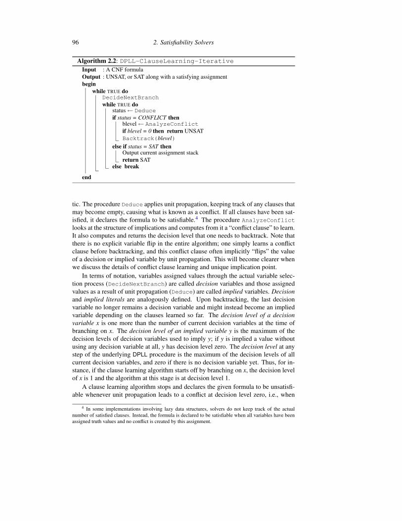
96 2. Satisfiability Solvers
Algorithm 2.2: DPLL-ClauseLearning-IterativeInput : A CNF formulaOutput : UNSAT, or SAT along with a satisfying assignmentbegin
while TRUE doDecideNextBranchwhile TRUE do
status← Deduceif status = CONFLICT then
blevel← AnalyzeConflictif blevel = 0 then return UNSATBacktrack(blevel)
else if status = SAT thenOutput current assignment stackreturn SAT
else breakend
tic. The procedure Deduce applies unit propagation, keeping track of any clauses thatmay become empty, causing what is known as a conflict. If all clauses have been sat-isfied, it declares the formula to be satisfiable.4 The procedure AnalyzeConflictlooks at the structure of implications and computes from it a “conflict clause” to learn.It also computes and returns the decision level that one needs to backtrack. Note thatthere is no explicit variable flip in the entire algorithm; one simply learns a conflictclause before backtracking, and this conflict clause often implicitly “flips” the valueof a decision or implied variable by unit propagation. This will become clearer whenwe discuss the details of conflict clause learning and unique implication point.
In terms of notation, variables assigned values through the actual variable selec-tion process (DecideNextBranch) are called decision variables and those assignedvalues as a result of unit propagation (Deduce) are called implied variables. Decisionand implied literals are analogously defined. Upon backtracking, the last decisionvariable no longer remains a decision variable and might instead become an impliedvariable depending on the clauses learned so far. The decision level of a decisionvariable x is one more than the number of current decision variables at the time ofbranching on x. The decision level of an implied variable y is the maximum of thedecision levels of decision variables used to imply y; if y is implied a value withoutusing any decision variable at all, y has decision level zero. The decision level at anystep of the underlying DPLL procedure is the maximum of the decision levels of allcurrent decision variables, and zero if there is no decision variable yet. Thus, for in-stance, if the clause learning algorithm starts off by branching on x, the decision levelof x is 1 and the algorithm at this stage is at decision level 1.
A clause learning algorithm stops and declares the given formula to be unsatisfi-able whenever unit propagation leads to a conflict at decision level zero, i.e., when
4 In some implementations involving lazy data structures, solvers do not keep track of the actualnumber of satisfied clauses. Instead, the formula is declared to be satisfiable when all variables have beenassigned truth values and no conflict is created by this assignment.

C.P. Gomes et al. 97
no variable is currently branched upon. This condition is sometimes referred to as aconflict at decision level zero.
Clause learning grew out of work in artificial intelligence seeking to improve theperformance of backtrack search algorithms by generating explanations for failure(backtrack) points, and then adding the explanations as new constraints on the originalproblem. The results of Davis [62], de Kleer and Williams [63], Dechter [64], Gene-sereth [82], Stallman and Sussman [220], and others proved this approach to be quitepromising. For general constraint satisfaction problems the explanations are called“conflicts” or “no-goods”; in the case of Boolean CNF satisfiability, the techniquebecomes clause learning—the reason for failure is learned in the form of a “conflictclause” which is added to the set of given clauses. Despite the initial success, the earlywork in this area was limited by the large numbers of no-goods generated during thesearch, which generally involved many variables and tended to slow the constraintsolvers down. Clause learning owes a lot of its practical success to subsequent re-search exploiting efficient lazy data structures and constraint database managementstrategies. Through a series of papers and often accompanying solvers, BayardoJr. and Miranker [17], Bayardo Jr. and Schrag [19], Marques-Silva and Sakallah[161], Moskewicz et al. [170], Zhang [236], Zhang et al. [240], and others showedthat clause learning can be efficiently implemented and used to solve hard problemsthat cannot be approached by any other technique.
In general, the learning process hidden in AnalyzeConflict is expected to saveus from redoing the same computation when we later have an assignment that causesconflict due in part to the same reason. Variations of such conflict-driven learninginclude different ways of choosing the clause to learn (different learning schemes)and possibly allowing multiple clauses to be learned from a single conflict. We nextformalize the graph-based framework used to define and compute conflict clauses.
Implication Graph and ConflictsUnit propagation can be naturally associated with an implication graph that capturesall possible ways of deriving all implied literals from decision literals. In what fol-lows, we use the term known clauses to refer to the clauses of the input formula aswell as to all clauses that have been learned by the clause learning process so far.
Definition 1. The implication graph G at a given stage of DPLL is a directed acyclicgraph with edges labeled with sets of clauses. It is constructed as follows:
Step 1: Create a node for each decision literal, labeled with that literal. Thesewill be the indegree-zero source nodes of G.
Step 2: While there exists a known clause C = (l1∨ . . . lk∨ l) such that¬l1, . . . ,¬lklabel nodes in G,
i. Add a node labeled l if not already present in G.ii. Add edges (li, l),1≤ i≤ k, if not already present.
iii. Add C to the label set of these edges. These edges are thought of asgrouped together and associated with clause C.

98 2. Satisfiability Solvers
Step 3: Add to G a special “conflict” node Λ. For any variable x that occurs bothpositively and negatively in G, add directed edges from x and ¬x to Λ.
Since all node labels in G are distinct, we identify nodes with the literals labelingthem. Any variable x occurring both positively and negatively in G is a conflict vari-able , and x as well as ¬x are conflict literals. G contains a conflict if it has at leastone conflict variable. DPLL at a given stage has a conflict if the implication graph atthat stage contains a conflict. A conflict can equivalently be thought of as occurringwhen the residual formula contains the empty clause Λ. Note that we are using Λ todenote the node of the implication graph representing a conflict, and Λ to denote theempty clause.
By definition, the implication graph may not contain a conflict at all, or it maycontain many conflict variables and several ways of deriving any single literal. Tobetter understand and analyze a conflict when it occurs, we work with a subgraph ofthe implication graph, called the conflict graph (see Figure 2.1), that captures only oneamong possibly many ways of reaching a conflict from the decision variables usingunit propagation.
a cut correspondingto clause (¬ a ∨ ¬ b)
¬ p
¬ q
b
a
¬ t
¬ x1
¬ x2
¬ x3
y
¬¬¬¬ y
Λ
reason side conflict side
conflictvariable
Figure 2.1: A conflict graph
Definition 2. A conflict graph H is any subgraph of the implication graph with thefollowing properties:
(a) H contains Λ and exactly one conflict variable.
(b) All nodes in H have a path to Λ.
(c) Every node l in H other than Λ either corresponds to a decision literal or hasprecisely the nodes¬l1,¬l2, . . . ,¬lk as predecessors where (l1∨ l2∨ . . .∨ lk∨ l)is a known clause.
While an implication graph may or may not contain conflicts, a conflict graphalways contains exactly one. The choice of the conflict graph is part of the strategyof the solver. A typical strategy will maintain one subgraph of an implication graphthat has properties (b) and (c) from Definition 2, but not property (a). This can be

C.P. Gomes et al. 99
thought of as a unique inference subgraph of the implication graph. When a conflictis reached, this unique inference subgraph is extended to satisfy property (a) as well,resulting in a conflict graph, which is then used to analyze the conflict.
Conflict clauses
For a subset U of the vertices of a graph, the edge-cut (henceforth called a cut) cor-responding to U is the set of all edges going from vertices in U to vertices not inU .
Consider the implication graph at a stage where there is a conflict and fix a conflictgraph contained in that implication graph. Choose any cut in the conflict graph thathas all decision variables on one side, called the reason side, and Λ as well as at leastone conflict literal on the other side, called the conflict side. All nodes on the reasonside that have at least one edge going to the conflict side form a cause of the conflict.The negations of the corresponding literals forms the conflict clause associated withthis cut.
Learning Schemes
The essence of clause learning is captured by the learning scheme used to analyze andlearn the “cause” of a failure. More concretely, different cuts in a conflict graph sep-arating decision variables from a set of nodes containing Λ and a conflict literal cor-respond to different learning schemes (see Figure 2.2). One may also define learningschemes based on cuts not involving conflict literals at all such as a scheme suggestedby Zhang et al. [240], but the effectiveness of such schemes is not clear. These willnot be considered here.
FirstNewCut clause(x1 ∨ x2 ∨ x3)
Decision clause(p ∨ q ∨ ¬ b)
1UIP clauset
rel-sat clause(¬ a ∨ ¬ b)
¬ p
¬ q
b
a
¬ t
¬ x1
¬ x2
¬ x3
y
¬¬¬¬ y
Λ
Figure 2.2: Learning schemes corresponding to different cuts in the conflict graph
It is insightful to think of the nondeterministic scheme as the most general learn-ing scheme. Here we select the cut nondeterministically, choosing, whenever pos-sible, one whose associated clause is not already known. Since we can repeatedlybranch on the same last variable, nondeterministic learning subsumes learning mul-tiple clauses from a single conflict as long as the sets of nodes on the reason side ofthe corresponding cuts form a (set-wise) decreasing sequence. For simplicity, we willassume that only one clause is learned from any conflict.

100 2. Satisfiability Solvers
In practice, however, we employ deterministic schemes. The decision scheme[240], for example, uses the cut whose reason side comprises all decision variables.Relsat [19] uses the cut whose conflict side consists of all implied variables at thecurrent decision level. This scheme allows the conflict clause to have exactly onevariable from the current decision level, causing an automatic flip in its assignmentupon backtracking. In the example depicted in Figure 2.2, the decision clause (p∨q∨¬b) has b as the only variable from the current decision level. After learning thisconflict clause and backtracking by unassigning b, the truth values of p and q (bothFALSE) immediately imply ¬b, flipping the value of b from TRUE to FALSE.
This nice flipping property holds in general for all unique implication points(UIPs) [161]. A UIP of an implication graph is a node at the current decision leveld such that every path from the decision variable at level d to the conflict variable orits negation must go through it. Intuitively, it is a single reason at level d that causesthe conflict. Whereas relsat uses the decision variable as the obvious UIP, Grasp[161] and zChaff [170] use FirstUIP, the one that is “closest” to the conflict variable.Grasp also learns multiple clauses when faced with a conflict. This makes it typicallyrequire fewer branching steps but possibly slower because of the time lost in learningand unit propagation.
The concept of UIP can be generalized to decision levels other than the currentone. The 1UIP scheme corresponds to learning the FirstUIP clause of the current de-cision level, the 2UIP scheme to learning the FirstUIP clauses of both the current leveland the one before, and so on. Zhang et al. [240] present a comparison of all theseand other learning schemes and conclude that 1UIP is quite robust and outperformsall other schemes they consider on most of the benchmarks.
Another learning scheme, which underlies the proof of a theorem to be presentedin the next section, is the FirstNewCut scheme [22]. This scheme starts with the cutthat is closest to the conflict literals and iteratively moves it back toward the decisionvariables until a conflict clause that is not already known is found; hence the nameFirstNewCut.
2.2.4 A Proof Complexity PerspectivePropositional proof complexity is the study of the structure of proofs of validity ofmathematical statements expressed in a propositional or Boolean form. Cook andReckhow [52] introduced the formal notion of a proof system in order to study math-ematical proofs from a computational perspective. They defined a propositional proofsystem to be an efficient algorithm A that takes as input a propositional statement Sand a purported proof π of its validity in a certain pre-specified format. The crucialproperty of A is that for all invalid statements S, it rejects the pair (S,π) for all π ,and for all valid statements S, it accepts the pair (S,π) for some proof π . This notionof proof systems can be alternatively formulated in terms of unsatisfiable formulas—those that are FALSE for all assignments to the variables.
They further observed that if there is no propositional proof system that admitsshort (polynomial in size) proofs of validity of all tautologies, i.e., if there exist com-putationally hard tautologies for every propositional proof system, then the complex-ity classes NP and co-NP are different, and hence P 6= NP. This observation makesfinding tautological formulas (equivalently, unsatisfiable formulas) that are computa-

C.P. Gomes et al. 101
tionally difficult for various proof systems one of the central tasks of proof complexityresearch, with far reaching consequences to complexity theory and Computer Sciencein general. These hard formulas naturally yield a hierarchy of proof systems based onthe sizes of proofs they admit. Tremendous amount of research has gone into under-standing this hierarchical structure. Beame and Pitassi [23] summarize many of theresults obtained in this area.
To understand current complete SAT solvers, we focus on the proof system calledresolution, denoted henceforth as RES. It is a very simple system with only one rulewhich applies to disjunctions of propositional variables and their negations: (a OR B)and ((NOT a) OR C) together imply (B OR C). Repeated application of this rulesuffices to derive an empty disjunction if and only if the initial formula is unsatisfiable;such a derivation serves as a proof of unsatisfiability of the formula.
Despite its simplicity, unrestricted resolution as defined above (also called gen-eral resolution) is hard to implement efficiently due to the difficulty of finding goodchoices of clauses to resolve; natural choices typically yield huge storage require-ments. Various restrictions on the structure of resolution proofs lead to less powerfulbut easier to implement refinements that have been studied extensively in proof com-plexity. Those of special interest to us are tree-like resolution, where every derivedclause is used at most once in the refutation, and regular resolution, where everyvariable is resolved upon at most one in any “path” from the initial clauses to theempty clause. While these and other refinements are sound and complete as proofsystems, they differ vastly in efficiency. For instance, in a series of results, Bonetet al. [34], Bonet and Galesi [35], and Buresh-Oppenheim and Pitassi [41] have shownthat regular, ordered, linear, positive, negative, and semantic resolution are all expo-nentially stronger than tree-like resolution. On the other hand, Bonet et al. [34] andAlekhnovich et al. [7] have proved that tree-like, regular, and ordered resolution areexponentially weaker than RES.
Most of today’s complete SAT solvers implement a subset of the resolution proofsystem. However, till recently, it wasn’t clear where exactly do they fit in the proofsystem hierarchy and how do they compare to refinements of resolution such as reg-ular resolution. Clause learning and random restarts can be considered to be twoof the most important ideas that have lifted the scope of modern SAT solvers fromexperimental toy problems to large instances taken from real world challenges. De-spite overwhelming empirical evidence, for many years not much was known of theultimate strengths and weaknesses of the two.
Beame, Kautz, and Sabharwal [22, 199] answered several of these questions in aformal proof complexity framework. They gave the first precise characterization ofclause learning as a proof system called CL and began the task of understanding itspower by relating it to resolution. In particular, they showed that with a new learningscheme called FirstNewCut, clause learning can provide exponentially shorter proofsthan any proper refinement of general resolution satisfying a natural self-reductionproperty. These include regular and ordered resolution, which are already known tobe much stronger than the ordinary DPLL procedure which captures most of the SATsolvers that do not incorporate clause learning. They also showed that a slight variantof clause learning with unlimited restarts is as powerful as general resolution itself.
From the basic proof complexity point of view, only families of unsatisfiable for-mulas are of interest because only proofs of unsatisfiability can be large; minimum

102 2. Satisfiability Solvers
proofs of satisfiability are linear in the number of variables of the formula. In prac-tice, however, many interesting formulas are satisfiable. To justify the approach ofusing a proof system CL, we refer to the work of Achlioptas, Beame, and Molloy [2]who have shown how negative proof complexity results for unsatisfiable formulas canbe used to derive run time lower bounds for specific inference algorithms, especiallyDPLL, running on satisfiable formulas as well. The key observation in their workis that before hitting a satisfying assignment, an algorithm is very likely to explorea large unsatisfiable part of the search space that results from the first bad variableassignment.
Proof complexity does not capture everything we intuitively mean by the powerof a reasoning system because it says nothing about how difficult it is to find short-est proofs. However, it is a good notion with which to begin our analysis becausethe size of proofs provides a lower bound on the running time of any implementationof the system. In the systems we consider, a branching function, which determineswhich variable to split upon or which pair of clauses to resolve, guides the search. Anegative proof complexity result for a system (“proofs must be large in this system”)tells us that a family of formulas is intractable even with a perfect branching func-tion; likewise, a positive result (“small proofs exist”) gives us hope of finding a goodbranching function, i.e., a branching function that helps us uncover a small proof.
We begin with an easy to prove relationship between DPLL (without clause learn-ing) and tree-like resolution (for a formal proof, see e.g. [199]).
Proposition 1. For a CNF formula F, the size of the smallest DPLL refutation of F isequal to the size of the smallest tree-like resolution refutation of F.
The interesting part is to understand what happens when clause learning is broughtinto the picture. It has been previously observed by Lynce and Marques-Silva [157]that clause learning can be viewed as adding resolvents to a tree-like resolution proof.The following results show further that clause learning, viewed as a propositionalproof system CL, is exponentially stronger than tree-like resolution. This explains,formally, the performance gains observed empirically when clause learning is addedto DPLL based solvers.
Clause Learning ProofsThe notion of clause learning proofs connects clause learning with resolution andprovides the basis for the complexity bounds to follow. If a given formula F is unsat-isfiable, the clause learning based DPLL process terminates with a conflict at decisionlevel zero. Since all clauses used in this final conflict themselves follow directly orindirectly from F , this failure of clause learning in finding a satisfying assignmentconstitutes a logical proof of unsatisfiability of F . In an informal sense, we denote byCL the proof system consisting of all such proofs; this can be made precise using thenotion of a branching sequence [22]. The results below compare the sizes of proofs inCL with the sizes of (possibly restricted) resolution proofs. Note that clause learningalgorithms can use one of many learning schemes, resulting in different proofs.
We next define what it means for a refinement of a proof system to be natural andproper. Let CS(F) denote the length of a shortest refutation of a formula F under aproof system S.

C.P. Gomes et al. 103
Definition 3 ([22, 199]). For proof systems S and T , and a function f : N→ [1,∞),
• S is natural if for any formula F and restriction ρ on its variables, CS(F |ρ) ≤CS(F).
• S is a refinement of T if proofs in S are also (restricted) proofs in T .
• S is f (n)-proper as a refinement of T if there exists a witnessing family Fnof formulas such that CS(Fn)≥ f (n) ·CT (Fn). The refinement is exponentially-proper if f (n) = 2nΩ(1) and super-polynomially-proper if f (n) = nω(1).
Under this definition, tree-like, regular, linear, positive, negative, semantic, andordered resolution are natural refinements of RES, and further, tree-like, regular, andordered resolution are exponentially-proper [7, 34].
Now we are ready to state the somewhat technical theorem relating the clauselearning process to resolution, whose corollaries are nonetheless easy to understand.The proof of this theorem is based on an explicit construction of so-called “proof-traceextension” formulas, which interestingly allow one to translate any known separationresult between RES and a natural proper refinement S of RES into a separation be-tween CL and S.
Theorem 1 ([22, 199]). For any f (n)-proper natural refinement S of RES and for CLusing the FirstNewCut scheme and no restarts, there exist formulas Fn such thatCS(Fn)≥ f (n) ·CCL(Fn).
Corollary 1. CL can provide exponentially shorter proofs than tree-like, regular, andordered resolution.
Corollary 2. Either CL is not a natural proof system or it is equivalent in strength toRES.
We remark that this leaves open the possibility that CL may not be able to simulateall regular resolution proofs. In this context, MacKenzie [158] has used argumentssimilar to those of Beame et al. [20] to prove that a natural variant of clause learningcan indeed simulate all of regular resolution.
Finally, let CL-- denote the variant of CL where one is allowed to branch on a literalwhose value is already set explicitly or because of unit propagation. Of course, sucha relaxation is useless in ordinary DPLL; there is no benefit in branching on a variablethat doesn’t even appear in the residual formula. However, with clause learning, sucha branch can lead to an immediate conflict and allow one to learn a key conflict clausethat would otherwise have not been learned. This property can be used to prove thatRES can be efficiently simulated by CL-- with enough restarts. In this context, a clauselearning scheme will be called non-redundant if on a conflict, it always learns a clausenot already known. Most of the practical clause learning schemes are non-redundant.
Theorem 2 ([22, 199]). CL-- with any non-redundant scheme and unlimited restartsis polynomially equivalent to RES.
We note that by choosing the restart points in a smart way, CL together withrestarts can be converted into a complete algorithm for satisfiability testing, i.e., for

104 2. Satisfiability Solvers
all unsatisfiable formulas given as input, it will halt and provide a proof of unsatis-fiability [16, 102]. The theorem above makes a much stronger claim about a slightvariant of CL, namely, with enough restarts, this variant can always find proofs ofunsatisfiability that are as short as those of RES.
2.2.5 Symmetry BreakingOne aspect of many theoretical as well as real-world problems that merits attention isthe presence of symmetry or equivalence amongst the underlying objects. Symmetrycan be defined informally as a mapping of a constraint satisfaction problem (CSP)onto itself that preserves its structure as well as its solutions. The concept of sym-metry in the context of SAT solvers and in terms of higher level problem objects isbest explained through some examples of the many application areas where it nat-urally occurs. For instance, in FPGA (field programmable gate array) routing usedin electronics design, all available wires or channels used for connecting two switchboxes are equivalent; in our design, it does not matter whether we use wire #1 be-tween connector X and connector Y, or wire #2, or wire #3, or any other availablewire. Similarly, in circuit modeling, all gates of the same “type” are interchangeable,and so are the inputs to a multiple fan-in AND or OR gate (i.e., a gate with several in-puts); in planning, all identical boxes that need to be moved from city A to city B areequivalent; in multi-processor scheduling, all available processors are equivalent; incache coherency protocols in distributed computing, all available identical caches areequivalent. A key property of such objects is that when selecting k of them, we canchoose, without loss of generality, any k. This without-loss-of-generality reasoning iswhat we would like to incorporate in an automatic fashion.
The question of symmetry exploitation that we are interested in addressing ariseswhen instances from domains such as the ones mentioned above are translated intoCNF formulas to be fed to a SAT solver. A CNF formula consists of constraints overdifferent kinds of variables that typically represent tuples of these high level objects(e.g. wires, boxes, etc.) and their interaction with each other. For example, duringthe problem modeling phase, we could have a Boolean variable zw,c that is TRUE iffthe first end of wire w is attached to connector c. When this formula is convertedinto DIMACS format for a SAT solver, the semantic meaning of the variables, that,say, variable 1324 is associated with wire #23 and connector #5, is discarded. Con-sequently, in this translation, the global notion of the obvious interchangeability ofthe set of wire objects is lost, and instead manifests itself indirectly as a symmetrybetween the (numbered) variables of the formula and therefore also as a symmetrywithin the set of satisfying (or un-satisfying) variable assignments. These sets ofsymmetric satisfying and un-satisfying assignments artificially explode both the sat-isfiable and the unsatisfiable parts of the search space, the latter of which can be achallenging obstacle for a SAT solver searching for a satisfying assignment.
One of the most successful techniques for handling symmetry in both SAT andgeneral CSPs originates from the work of Puget [187], who showed that symme-tries can be broken by adding one lexicographic ordering constraint per symmetry.Crawford et al. [55] showed how this can be done by adding a set of simple “lex-constraints” or symmetry breaking predicates (SBPs) to the input specification toweed out all but the lexically-first solutions. The idea is to identify the group of

C.P. Gomes et al. 105
permutations of variables that keep the CNF formula unchanged. For each such per-mutation π , clauses are added so that for every satisfying assignment σ for the originalproblem, whose permutation π(σ) is also a satisfying assignment, only the lexically-first of σ and π(σ) satisfies the added clauses. In the context of CSPs, there has beena lot of work in the area of SBPs. Petrie and Smith [182] extended the idea to valuesymmetries, Puget [189] applied it to products of variable and value symmetries, andWalsh [231] generalized the concept to symmetries acting simultaneously on vari-ables and values, on set variables, etc. Puget [188] has recently proposed a techniquefor creating dynamic lex-constraints, with the goal of minimizing adverse interactionwith the variable ordering used in the search tree.
In the context of SAT, value symmetries for the high-level variables naturally man-ifest themselves as low-level variable symmetries, and work on SBPs has taken adifferent path. Tools such as Shatter by Aloul et al. [8] improve upon the basicSBP technique by using lex-constraints whose size is only linear in the number ofvariables rather than quadratic. Further, they use graph isomorphism detectors likeSaucy by Darga et al. [56] to generate symmetry breaking predicates only for thegenerators of the algebraic groups of symmetry. This latter problem of computinggraph isomorphism, however, is not known to have any polynomial time algorithms,and is conjectured to be strictly between the complexity classes P and NP [cf. 136].Hence, one must resort to heuristic or approximate solutions. Further, while there areformulas for which few SBPs suffice, the number of SBPs one needs to add in orderto break all symmetries can be exponential. This is typically handled in practice bydiscarding “large” symmetries, i.e., those involving too many variables with respect toa fixed threshold. This may, however, sometimes result in much slower SAT solutionsin domains such as clique coloring and logistics planning.
A very different and indirect approach for addressing symmetry is embodied inSAT solvers such as PBS by Aloul et al. [9], pbChaff by Dixon et al. [68], andGalena by Chai and Kuehlmann [44], which utilize non-CNF formulations knownas pseudo-Boolean inequalities. Their logic reasoning is based on what is called theCutting Planes proof system which, as shown by Cook et al. [53], is strictly strongerthan resolution on which DPLL type CNF solvers are based. Since this more powerfulproof system is difficult to implement in its full generality, pseudo-Boolean solversoften implement only a subset of it, typically learning only CNF clauses or restrictedpseudo-Boolean constraints upon a conflict. Pseudo-Boolean solvers may lead topurely syntactic representational efficiency in cases where a single constraint such asy1 + y2 + . . .+ yk ≤ 1 is equivalent to
(k2)
binary clauses. More importantly, they arerelevant to symmetry because they sometimes allow implicit encoding. For instance,the single constraint x1 +x2 + . . .+xn ≤m over n variables captures the essence of thepigeonhole formula PHPn
m over nm variables which is provably exponentially hard tosolve using resolution-based methods without symmetry considerations [108]. Thisimplicit representation, however, is not suitable in certain applications such as cliquecoloring and planning that we discuss. In fact, for unsatisfiable clique coloring in-stances, even pseudo-Boolean solvers provably require exponential time.
One could conceivably keep the CNF input unchanged but modify the solver todetect and handle symmetries during the search phase as they occur. Although thisapproach is quite natural, we are unaware of its implementation in a general purposeSAT solver besides sEqSatz by Li et al. [151], which has been shown to be effective

106 2. Satisfiability Solvers
on matrix multiplication and polynomial multiplication problems. Symmetry han-dling during search has been explored with mixed results in the CSP domain usingframeworks like SBDD and SBDS [e.g. 72, 73, 84, 87]. Related work in SAT hasbeen done in the specific areas of automatic test pattern generation by Marques-Silvaand Sakallah [162] and SAT-based model checking by Shtrichman [214]. In bothcases, the solver utilizes global information obtained at a stage to make subsequentstages faster. In other domain-specific work on symmetries in problems relevant toSAT, Fox and Long [74] propose a framework for handling symmetry in planningproblems solved using the planning graph framework. They detect equivalence be-tween various objects in the planning instance and use this information to reduce thesearch space explored by their planner. Unlike typical SAT-based planners, this ap-proach does not guarantee plans of optimal length when multiple (non-conflicting)actions are allowed to be performed at each time step in parallel. Fortunately, thisissue does not arise in the SymChaff approach for SAT to be mentioned shortly.
Dixon et al. [67] give a generic method of representing and dynamically maintain-ing symmetry in SAT solvers using algebraic techniques that guarantee polynomialsize unsatisfiability proofs of many difficult formulas. The strength of their work liesin a strong group theoretic foundation and comprehensiveness in handling all possiblesymmetries. The computations involving group operations that underlie their currentimplementation are, however, often quite expensive.
When viewing complete SAT solvers as implementations of proof systems, thechallenge with respect to symmetry exploitation is to push the underlying proof sys-tem up in the weak-to-strong proof complexity hierarchy without incurring the signifi-cant cost that typically comes from large search spaces associated with complex proofsystems. While most of the current SAT solvers implement subsets of the resolutionproof system, a different kind of solver called SymChaff [199, 200] brings it up closerto symmetric resolution, a proof system known to be exponentially stronger than res-olution [139, 226]. More critically, it achieves this in a time- and space-efficientmanner. Interestingly, while SymChaff involves adding structure to the problem de-scription, it still stays within the realm of SAT solvers (as opposed to using a constraintprogramming (CP) approach), thereby exploiting the many benefits of the CNF formand the advances in state-of-the-art SAT solvers.
As a structure-aware solver, SymChaff incorporates several new ideas, includingsimple but effective symmetry representation, multiway branching based on variableclasses and symmetry sets, and symmetric learning as an extension of clause learningto multiway branches. Two key places where it differs from earlier approaches arein using high level problem description to obtain symmetry information (instead oftrying to recover it from the CNF formula) and in maintaining this information dy-namically but without using a complex group theoretic machinery. This allows it toovercome many drawbacks of previously proposed solutions. It is shown, in particu-lar, that straightforward annotation in the usual PDDL specification of planning prob-lems is enough to automatically and quickly generate relevant symmetry information,which in turn makes the search for an optimal plan several orders of magnitude faster.Similar performance gains are seen in other domains as well.
C.P. Gomes et al. 107
2.3 SAT Solver Technology—Incomplete Methods
An incomplete method for solving the SAT problem is one that does not providethe guarantee that it will eventually either report a satisfying assignment or provethe given formula unsatisfiable. Such a method is typically run with a pre-set limit,after which it may or may not produce a solution. Unlike the systematic solversbased on an exhaustive branching and backtracking search, incomplete methods aregenerally based on stochastic local search. On problems from a variety of domains,such incomplete methods for SAT can significantly outperform DPLL-based methods.Since the early 1990’s, there has been a tremendous amount of research on designing,understanding, and improving local search methods for SAT [e.g. 43, 77, 88, 89,104, 105, 109, 113, 114, 116, 132, 137, 152, 164, 180, 183, 191, 206, 219] as wellas on hybrid approaches that attempt to combine DPLL and local search methods[e.g. 10, 106, 163, 185, 195].5 We begin this section by discussing two methodsthat played a key role in the success of local search in SAT, namely GSAT [213] andWalksat [211]. We will then explore the phase transition phenomenon in randomSAT and a relatively new incomplete technique called Survey Propagation. We notethat there are also other exciting related solution techniques such as those based onLagrangian methods [207, 229, 235] and translation to integer programming [112,124].
The original impetus for trying a local search method on satisfiability problemswas the successful application of such methods for finding solutions to large N-queensproblems, first using a connectionist system by Adorf and Johnston [6], and then us-ing greedy local search by Minton et al. [167]. It was originally assumed that thissuccess simply indicated that N-queens was an easy problem, and researchers felt thatsuch techniques would fail in practice for SAT. In particular, it was believed that localsearch methods would easily get stuck in local minima, with a few clauses remainingunsatisfied. The GSAT experiments showed, however, that certain local search strate-gies often do reach global minima, in many cases much faster than systematic searchstrategies.
GSAT is based on a randomized local search technique [153, 177]. The basic GSATprocedure, introduced by Selman et al. [213] and described here as Algorithm 2.3,starts with a randomly generated truth assignment. It then greedily changes (‘flips’)the assignment of the variable that leads to the greatest decrease in the total numberof unsatisfied clauses. Such flips are repeated until either a satisfying assignment isfound or a pre-set maximum number of flips (MAX-FLIPS) is reached. This process isrepeated as needed, up to a maximum of MAX-TRIES times.
Selman et al. showed that GSAT substantially outperformed even the best back-tracking search procedures of the time on various classes of formulas, including ran-domly generated formulas and SAT encodings of graph coloring problems [123]. Thesearch of GSAT typically begins with a rapid greedy descent towards a better assign-ment, followed by long sequences of “sideways” moves, i.e., moves that do not in-crease or decrease the total number of unsatisfied clauses. In the search space, eachcollection of truth assignments that are connected together by a sequence of possible
5 As in our discussion of the complete SAT solvers, we cannot do justice to all recent research in localsearch solvers for SAT. We will again try to provide a brief overview and touch upon some interestingdetails.

108 2. Satisfiability Solvers
Algorithm 2.3: GSAT (F)
Input : A CNF formula FParameters : Integers MAX-FLIPS, MAX-TRIESOutput : A satisfying assignment for F , or FAILbegin
for i← 1 to MAX-TRIES doσ ← a randomly generated truth assignment for Ffor j← 1 to MAX-FLIPS do
if σ satisfies F then return σ // successv← a variable flipping which results in the greatest decrease
(possibly negative) in the number of unsatisfied clausesFlip v in σ
return FAIL // no satisfying assignment foundend
sideways moves is referred to as a plateau. Experiments indicate that on many for-mulas, GSAT spends most of its time moving from plateau to plateau. Interestingly,Frank et al. [77] observed that in practice, almost all plateaus do have so-called “exits”that lead to another plateau with a lower number of unsatisfied clauses. Intuitively,in a very high dimensional search space such as the space of a 10,000 variable for-mula, it is very rare to encounter local minima, which are plateaus from where thereis no local move that decreases the number of unsatisfied clauses. In practice, thismeans that GSAT most often does not get stuck in local minima, although it may takea substantial amount of time on each plateau before moving on to the next one. Thismotivates studying various modifications in order to speed up this process [209, 210].One of the most successful strategies is to introduce noise into the search in the formof uphill moves, which forms the basis of the now well-known local search methodfor SAT called Walksat [211].
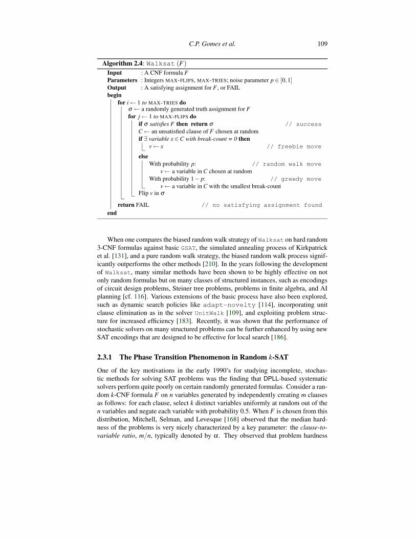
Walksat interleaves the greedy moves of GSAT with random walk moves of astandard Metropolis search. It further focuses the search by always selecting the vari-able to flip from an unsatisfied clause C (chosen at random). If there is a variable in Cflipping which does not turn any currently satisfied clauses to unsatisfied, it flips thisvariable (a “freebie” move). Otherwise, with a certain probability, it flips a randomliteral of C (a “random walk” move), and with the remaining probability, it flips avariable in C that minimizes the break-count, i.e., the number of currently satisfiedclauses that become unsatisfied (a “greedy” move). Walksat is presented in detailas Algorithm 2.4. One of its parameters, in addition to the maximum number of triesand flips, is the noise p ∈ [0,1], which controls how often are non-greedy moves con-sidered during the stochastic search. It has been found empirically that for variousproblems from a single domain, a single value of p is optimal.
The focusing strategy of Walksat based on selecting variables solely from un-satisfied clauses was inspired by the O(n2) randomized algorithm for 2-SAT by Pa-padimitriou [178]. It can be shown that for any satisfiable formula and starting fromany truth assignment, there exists a sequence of flips using only variables from unsat-isfied clauses such that one obtains a satisfying assignment.
C.P. Gomes et al. 109
Algorithm 2.4: Walksat (F)
Input : A CNF formula FParameters : Integers MAX-FLIPS, MAX-TRIES; noise parameter p ∈ [0,1]Output : A satisfying assignment for F , or FAILbegin
for i← 1 to MAX-TRIES doσ ← a randomly generated truth assignment for Ffor j← 1 to MAX-FLIPS do
if σ satisfies F then return σ // successC← an unsatisfied clause of F chosen at randomif ∃ variable x ∈C with break-count = 0 then
v← x // freebie move
elseWith probability p: // random walk move
v← a variable in C chosen at randomWith probability 1− p: // greedy move
v← a variable in C with the smallest break-countFlip v in σ
return FAIL // no satisfying assignment foundend
When one compares the biased random walk strategy of Walksat on hard random3-CNF formulas against basic GSAT, the simulated annealing process of Kirkpatricket al. [131], and a pure random walk strategy, the biased random walk process signif-icantly outperforms the other methods [210]. In the years following the developmentof Walksat, many similar methods have been shown to be highly effective on notonly random formulas but on many classes of structured instances, such as encodingsof circuit design problems, Steiner tree problems, problems in finite algebra, and AIplanning [cf. 116]. Various extensions of the basic process have also been explored,such as dynamic search policies like adapt-novelty [114], incorporating unitclause elimination as in the solver UnitWalk [109], and exploiting problem struc-ture for increased efficiency [183]. Recently, it was shown that the performance ofstochastic solvers on many structured problems can be further enhanced by using newSAT encodings that are designed to be effective for local search [186].
2.3.1 The Phase Transition Phenomenon in Random k-SATOne of the key motivations in the early 1990’s for studying incomplete, stochas-tic methods for solving SAT problems was the finding that DPLL-based systematicsolvers perform quite poorly on certain randomly generated formulas. Consider a ran-dom k-CNF formula F on n variables generated by independently creating m clausesas follows: for each clause, select k distinct variables uniformly at random out of then variables and negate each variable with probability 0.5. When F is chosen from thisdistribution, Mitchell, Selman, and Levesque [168] observed that the median hard-ness of the problems is very nicely characterized by a key parameter: the clause-to-variable ratio, m/n, typically denoted by α . They observed that problem hardness
110 2. Satisfiability Solvers
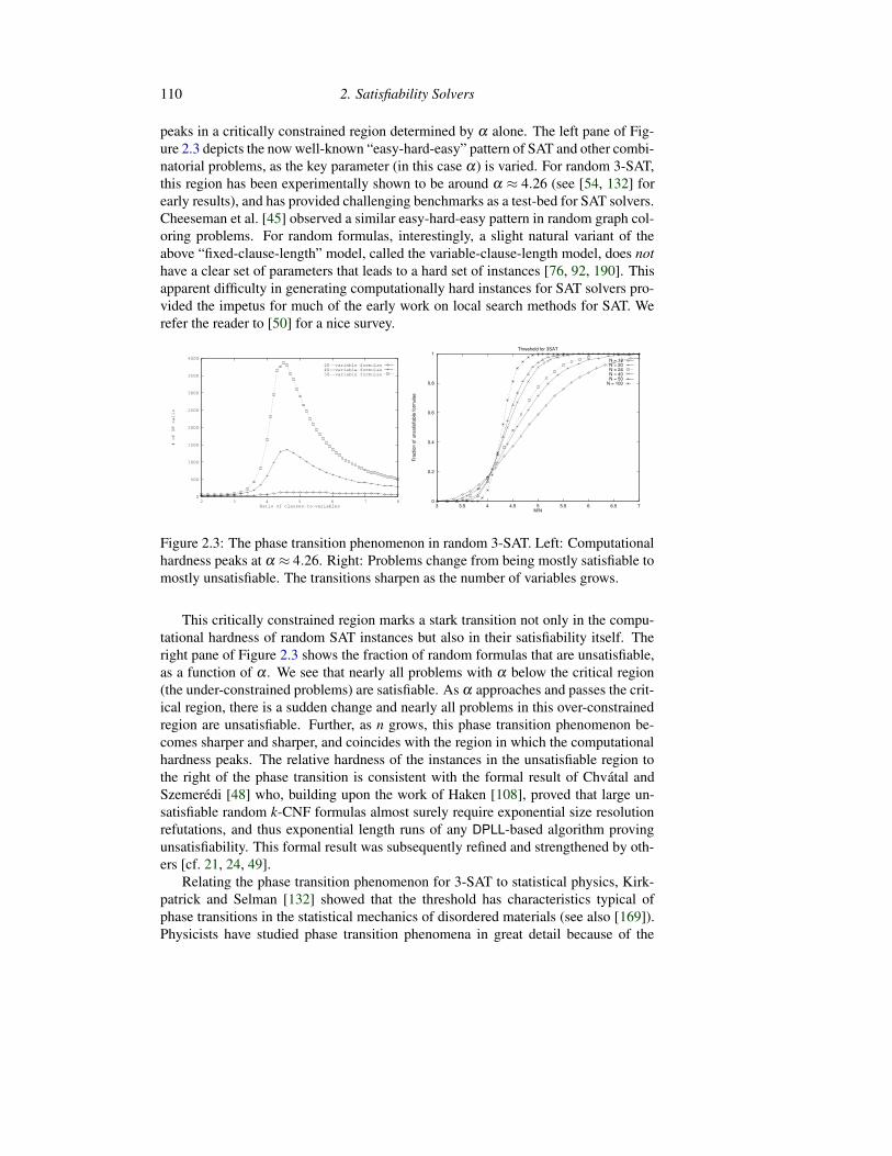
peaks in a critically constrained region determined by α alone. The left pane of Fig-ure 2.3 depicts the now well-known “easy-hard-easy” pattern of SAT and other combi-natorial problems, as the key parameter (in this case α) is varied. For random 3-SAT,this region has been experimentally shown to be around α ≈ 4.26 (see [54, 132] forearly results), and has provided challenging benchmarks as a test-bed for SAT solvers.Cheeseman et al. [45] observed a similar easy-hard-easy pattern in random graph col-oring problems. For random formulas, interestingly, a slight natural variant of theabove “fixed-clause-length” model, called the variable-clause-length model, does nothave a clear set of parameters that leads to a hard set of instances [76, 92, 190]. Thisapparent difficulty in generating computationally hard instances for SAT solvers pro-vided the impetus for much of the early work on local search methods for SAT. Werefer the reader to [50] for a nice survey.
0
500
1000
1500
2000
2500
3000
3500
4000
2 3 4 5 6 7 8
# of DP calls
Ratio of clauses-to-variables
20--variable formulas40--variable formulas50--variable formulas
0
0.2
0.4
0.6
0.8
1
3 3.5 4 4.5 5 5.5 6 6.5 7
Frac
tion
of u
nsat
isfia
ble
form
ulae
M/N
Threshold for 3SAT
N = 12N = 20N = 24N = 40N = 50
N = 100
Figure 2.3: The phase transition phenomenon in random 3-SAT. Left: Computationalhardness peaks at α ≈ 4.26. Right: Problems change from being mostly satisfiable tomostly unsatisfiable. The transitions sharpen as the number of variables grows.
This critically constrained region marks a stark transition not only in the compu-tational hardness of random SAT instances but also in their satisfiability itself. Theright pane of Figure 2.3 shows the fraction of random formulas that are unsatisfiable,as a function of α . We see that nearly all problems with α below the critical region(the under-constrained problems) are satisfiable. As α approaches and passes the crit-ical region, there is a sudden change and nearly all problems in this over-constrainedregion are unsatisfiable. Further, as n grows, this phase transition phenomenon be-comes sharper and sharper, and coincides with the region in which the computationalhardness peaks. The relative hardness of the instances in the unsatisfiable region tothe right of the phase transition is consistent with the formal result of Chvatal andSzemeredi [48] who, building upon the work of Haken [108], proved that large un-satisfiable random k-CNF formulas almost surely require exponential size resolutionrefutations, and thus exponential length runs of any DPLL-based algorithm provingunsatisfiability. This formal result was subsequently refined and strengthened by oth-ers [cf. 21, 24, 49].
Relating the phase transition phenomenon for 3-SAT to statistical physics, Kirk-patrick and Selman [132] showed that the threshold has characteristics typical ofphase transitions in the statistical mechanics of disordered materials (see also [169]).Physicists have studied phase transition phenomena in great detail because of the

C.P. Gomes et al. 111
many interesting changes in a system’s macroscopic behavior that occur at phaseboundaries. One useful tool for the analysis of phase transition phenomena is calledfinite-size scaling analysis. This approach is based on rescaling the horizontal axisby a factor that is a function of n. The function is such that the horizontal axis isstretched out for larger n. In effect, rescaling “slows down” the phase-transition forhigher values of n, and thus gives us a better look inside the transition. From the re-sulting universal curve, applying the scaling function backwards, the actual transitioncurve for each value of n can be obtained. In principle, this approach also localizesthe 50%-satisfiable-point for any value of n, which allows one to generate the hardestpossible random 3-SAT instances.
Interestingly, it is still not formally known whether there even exists a critical con-stant αc such that as n grows, almost all 3-SAT formulas with α < αc are satisfiableand almost all 3-SAT formulas with α > αc are unsatisfiable. In this respect, Friedgut[78] provided the first positive result, showing that there exists a function αc(n) de-pending on n such that the above threshold property holds. (It is quite likely that thethreshold in fact does not depend on n, and is a fixed constant.) In a series of papers,researchers have narrowed down the gap between upper bounds on the threshold for3-SAT [e.g. 40, 69, 76, 120, 133], the best so far being 4.596, and lower bounds [e.g.1, 5, 40, 75, 79, 107, 125], the best so far being 3.52. On the other hand, for random2-SAT, we do have a full rigorous understanding of the phase transition, which occursat clause-to-variable ratio of 1 [33, 47]. Also, for general k, the threshold for randomk-SAT is known to be in the range 2k ln2−O(k) [3, 101].
2.3.2 A New Technique for Random k-SAT: Survey PropagationWe end this section with a brief discussion of Survey Propagation (SP), an excitingnew algorithm for solving hard combinatorial problems. It was discovered in 2002 byMezard, Parisi, and Zecchina [165], and is so far the only known method successful atsolving random 3-SAT instances with one million variables and beyond in near-lineartime in the most critically constrained region.6
The SP method is quite radical in that it tries to approximate, using an iterativeprocess of local “message” updates, certain marginal probabilities related to the setof satisfying assignments. It then assigns values to variables with the most extremeprobabilities, simplifies the formula, and repeats the process. This strategy is referredto as SP-inspired decimation. In effect, the algorithm behaves like the usual DPLL-based methods, which also assign variable values incrementally in an attempt to find asatisfying assignment. However, quite surprisingly, SP almost never has to backtrack.In other words, the “heuristic guidance” from SP is almost always correct. Note that,interestingly, computing marginals on satisfying assignments is strongly believed tobe much harder than finding a single satisfying assignment (#P-complete vs. NP-complete). Nonetheless, SP is able to efficiently approximate certain marginals onrandom SAT instances and uses this information to successfully find a satisfying as-signment.
SP was derived from rather complex statistical physics methods, specifically, theso-called cavity method developed for the study of spin glasses. The method is still far
6 It has been recently shown that by finely tuning the noise parameter, Walksat can also be made toscale well on hard random 3-SAT instances, well above the clause-to-variable ratio of 4.2 [208].

112 2. Satisfiability Solvers
from well-understood, but in recent years, we are starting to see results that provideimportant insights into its workings [e.g. 4, 12, 39, 140, 159, 166]. Close connectionsto belief propagation (BP) methods [181] more familiar to computer scientists havebeen subsequently discovered. In particular, it was shown by Braunstein and Zecchina[39] (later extended by Maneva, Mossel, and Wainwright [159]) that SP equations areequivalent to BP equations for obtaining marginals over a special class of combinato-rial objects, called covers. In this respect, SP is the first successful example of the useof a probabilistic reasoning technique to solve a purely combinatorial search problem.The recent work of Kroc et al. [140] empirically established that SP, despite the veryloopy nature of random formulas which violate the standard tree-structure assump-tions underlying the BP algorithm, is remarkably good at computing marginals overthese covers objects on large random 3-SAT instances.
Unfortunately, the success of SP is currently limited to random SAT instances. Itis an exciting research challenge to further understand SP and apply it successfully tomore structured, real-world problem instances.
2.4 Runtime Variance and Problem Structure
The performance of backtrack-style search methods can vary dramatically dependingon the way one selects the next variable to branch on (the “variable selection heuris-tic”) and in what order the possible values are assigned to the variable (the “valueselection heuristic”). The inherent exponential nature of the search process appearsto magnify the unpredictability of search procedures. In fact, it is not uncommon toobserve a backtrack search procedure “hang” on a given instance, whereas a differentheuristic, or even just another randomized run, solves the instance quickly. A relatedphenomenon is observed in random problem distributions that exhibit an “easy-hard-easy” pattern in computational complexity, concerning so-called “exceptionally hard”instances: such instances seem to defy the “easy-hard-easy” pattern. They occur inthe under-constrained area, but they seem to be considerably harder than other similarinstances and even harder than instances from the critically constrained area. Thisphenomenon was first identified by Hogg and Willimans in graph coloring [111] andby Gent and Walsh in satisfiability problems [83]. An instance is considered to be ex-ceptionally hard, for a particular search algorithm, when it occurs in the region wherealmost all problem instances are satisfiable (i.e., the under constrained area), but isconsiderably harder to solve than other similar instances, and even harder than mostof the instances in the critically constrained area [83, 111, 217]. However, subse-quent research showed that such instances are not inherently difficult; for example,by simply renaming the variables or by considering a different search heuristic suchinstances can be easily solved [212, 218]. Therefore, the “hardness” of exceptionallyhard instances does not reside in the instances per se, but rather in the combina-tion of the instance with the details of the search method. This is the reason whyresearchers studying the hardness of computational problems use the median to char-acterize search difficulty, instead of the mean, since the behavior of the mean tends tobe quite erratic [95].

C.P. Gomes et al. 113
2.4.1 Fat and Heavy Tailed behaviorThe study of the full runtime distributions of search methods—instead of just the mo-ments and median—has been shown to provide a better characterization of searchmethods and much useful information in the design of algorithms. In particular,researchers have shown that the runtime distributions of complete backtrack searchmethods reveal intriguing characteristics of such search methods: quite often com-plete backtrack search methods exhibit fat and heavy-tailed behavior [80, 95, 111].Such runtime distributions can be observed when running a deterministic backtrack-ing procedure on a distribution of random instances, and perhaps more importantlyby repeated runs of a randomized backtracking procedure on a single instance.
The notion of fat-tailedness is based on the concept of kurtosis. The kurtosisis defined as µ4/µ2
2 (µ4 is the fourth central moment about the mean and µ2 is thesecond central moment about the mean, i.e., the variance). If a distribution has a highcentral peak and long tails, than the kurtosis is in general large. The kurtosis of thestandard normal distribution is 3. A distribution with a kurtosis larger than 3 is fat-tailed or leptokurtic. Examples of distributions that are characterized by fat-tails arethe exponential distribution, the lognormal distribution, and the Weibull distribution.
Heavy-tailed distributions have “heavier” tails than fat-tailed distributions; in factthey have some infinite moments, e.g., they can have infinite mean, infinite variance,etc. More rigorously, a random variable X with probability distribution function F(·)is heavy-tailed if it has the so-called Pareto like decay of the tails, i.e.:
1−F(x) = Pr[X > x]∼Cx−α , x > 0,
where α > 0 and C > 0 are constants. When 1 < α < 2, X has infinite variance,and infinite mean and variance when 0 < α <= 1. The log-log plot of 1−F(x) of aPareto-like distribution (i.e., the survival function) shows linear behavior with slopedetermined by α . Like heavy-tailed distributions, fat-tailed distributions have longtails, with a considerable mass of probability concentrated in the tails. Nevertheless,the tails of fat-tailed distributions are lighter than heavy-tailed distributions.
DPLL style complete backtrack search methods have been shown to exhibit heavy-tailed behavior, both in random instances and real-world instances. Example domainsare QCP [95], scheduling [97], planning[102], model checking, and graph coloring[122, 230]. Several formal models generating heavy-tailed behavior in search havebeen proposed [46, 94, 122, 233, 234]. If the runtime distribution of a backtracksearch method is heavy-tailed, it will produce runs spanning over several orders ofmagnitude, some extremely long but also some extremely short. Methods like ran-domization and restarts try to exploit this phenomenon [102].
2.4.2 BackdoorsInsight into heavy-tailed behavior comes from considering backdoor variables. Theseare variables which, when set, give us a polynomial subproblem. Intuitively, a smallbackdoor set explains how a backtrack search method can get “lucky” on certain runs,where backdoor variables are identified early on in the search and set the right way.Formally, the definition of a backdoor depends on a particular algorithm, referred to

114 2. Satisfiability Solvers
as sub-solver, that solves a tractable sub-case of the general constraint satisfactionproblem [233].
Definition 4. A sub-solver A given as input a CSP, C, satisfies the following:
i. Trichotomy: A either rejects the input C, or “determines” C correctly (as unsatis-fiable or satisfiable, returning a solution if satisfiable),
ii. Efficiency: A runs in polynomial time,
iii. Trivial solvability: A can determine if C is trivially true (has no constraints) ortrivially false (has a contradictory constraint),
iv. Self-reducibility: if A determines C, then for any variable x and value v, A deter-mines C[v/x].7
For instance, A could be an algorithm that enforces arc consistency. Using thedefinition of sub-solver we can now formally define the concept of backdoor set. LetA be a sub-solver and C be a CSP. A nonempty subset S of the variables with domainD is a (weak) backdoor in C for A if for some aS : S→ D, A returns a satisfyingassignment of C[aS]. Intuitively, the backdoor corresponds to a set of variables, suchthat when set correctly, the sub-solver can solve the remaining problem. A strongernotion of backdoors considers both satisfiable and unsatisfiable (inconsistent) probleminstances. A nonempty subset S of the variables is a strong backdoor in C for A if forall aS : S→D, A returns a satisfying assignment or concludes unsatisfiability of C[aS].
Szeider [223] considered the parameterized complexity of the problem of deter-mining whether a SAT instance has a weak or strong backdoor set of size k or less forDPLL style sub-solvers, i.e., subsolvers based on unit propagation and/or pure literalelimination. He showed that detection of weak and strong backdoor sets is unlikely tobe fixed-parameter tractable. Nishimura et al. [172] provided more positive results fordetecting backdoor sets where the sub-solver solves Horn or 2-CNF formulas, bothof which are linear time problems. They proved that the detection of such a strongbackdoor set is fixed-parameter tractable, while the detection of a weak backdoor setis not. The explanation that they offered for such a discrepancy is quite interesting:for strong backdoor sets one only has to guarantee that the chosen set of variablesgives a subproblem within the chosen syntactic class; for weak backdoor sets, onealso has to guarantee satisfiability of the simplified formula, a property that cannot bedescribed syntactically.
Dilkina et al. [66] studied the tradeoff between the complexity of backdoor de-tection and the backdoor size. They proved that adding certain obvious inconsistencychecks to the underlying class can make the complexity of backdoor detection jumpfrom being within NP to being both NP-hard and coNP-hard. On the positive side,they showed that this change can dramatically reduce the size of the resulting back-doors. They also explored the differences between so-called deletion backdoors andstrong backdoors, in particular with respect to the class of renamable Horn formulas.
Concerning the size of backdoors, random formulas do not appear to have smallbackdoor sets. For example, for random 3-SAT problems near the phase transition,the backdoor size appears to be a constant fraction (roughly 30%) of the total number
7We use C[v/x] to denote the simplified CSP obtained by setting the value of variable x to v in C.

C.P. Gomes et al. 115
of variables [119]. This may explain why the current DPLL based solvers have notmade significant progress on hard randomly generated instances. Empirical resultsbased on real-world instances suggest a more positive picture. Structured probleminstances can have surprisingly small sets of backdoor variables, which may explainwhy current state-of-the-art solvers are able to solve very large real-world instances.For example the logistics-d planning problem instance (log.d) has a backdoor set ofjust 12 variables, compared to a total of nearly 7,000 variables in the formula, usingthe polynomial time propagation techniques of the SAT solver Satz [148]. Hoffmannet al. [110] proved the existence of strong backdoor sets of size just O(logn) forcertain families of logistics planning problems and blocks world problems.
Figure 2.4: Constraint graph of a real-world instance from the logistics planning do-main. The instance in the plot has 843 vars and 7,301 clauses. One backdoor set forthis instance w.r.t. unit propagation has size 16 (not necessarily the minimum back-door set). Left: Constraint graph of the original instance. Center: Constraint graphafter setting 5 variables and performing unit propagation. Right: Constraint graphafter setting 14 variables and performing unit propagation.
Even though computing minimum backdoor sets is worst-case intractable [223], ifwe bound the size of the backdoor, heuristics and techniques like randomization andrestarts can often uncover a small backdoor in practice [130]. In fact, state-of-the-art SAT solvers are surprisingly effective in finding small backdoors in many struc-tured problem instances. Figure 2.4 shows a visualization of the constraint graph ofa logistics planning problem and how this graph is drastically simplified after onlya few variables occurring in a small backdoor (found by SAT solvers) are set. Inrelated work, Slaney and Walsh [216] studied the structural notion of “backbones”and Dequen and Dubois introduced a heuristic for DPLL based solvers that exploitsthe notion of backbone and outperforms other heuristics on random 3-SAT problems[65, 70].
2.4.3 RestartsOne way to exploit heavy-tailed behavior is to add restarts to a backtracking proce-dure. A sequence of short runs instead of a single long run may be a more effective useof computational resources (see Figure 2.5). Gomes et al. proposed randomized rapidrestarts (RRR) to take advantage of heavy-tailed behavior and boost the efficiency of

116 2. Satisfiability Solvers
complete backtrack search procedures [102]. In practice, one gradually increases thecutoff to maintain completeness [16, 102]. Gomes et al. showed that a restart strategywith a fixed cutoff eliminates heavy-tail behavior and has finite moments [96].
Prior to the discovery of heavy-tailed behavior and backdoor sets, randomizedrestart policies have been studied in the context of general randomized Las Vegasprocedures. Luby et al. [155] showed that when the underlying runtime distributionof the randomized procedure is fully known, the optimal restart policy is a fixed cut-off. When there is no a priori knowledge about the distribution, they also provideda universal strategy which minimizes the expected cost. This consists of runs whoselengths are powers of two, and each time a pair of runs of a given length has beencompleted, a run of twice that length is immediately executed. The universal strategyis of the form: 1,1,2,1,1,2,4,1,1,2,4,8, · · ·. Although the universal strategy of Lubyet al. is provably within a log factor of the optimal fixed cutoff, the schedule oftenconverges too slowly in practice. Walsh [230] introduced a restart strategy, inspiredby Luby et al.’s analysis, in which the cutoff value increases geometrically. The ad-vantage of such a strategy is that it is less sensitive to the details of the underlyingdistribution. Following the findings of Gomes et al. [102] and starting with zChaff,state-of-the-art SAT solvers now routinely use restarts. In practice, the solvers use adefault cutoff value, which is increased, linearly, every given number of restarts, guar-anteeing the completeness of the solver in the limit [170]. Another important featureis that they retain learned clauses across restarts.
0.0001
0.001
0.01
0.1
1
1 10 100 1000
fraction u
nsolv
ed
total number of backtracks
effect of restarts (cutoff 4)
no restarts
with restarts
23
1000
10000
100000
1000000
1 10 100 1000 10000 100000 1000000log( cutoff )
log
( b
acktr
acks )
(a) (b)
Figure 2.5: Restarts: (a) Tail (1−F(x)) as a function of the total number of backtracksfor a QCP instance, log-log scale; the lower curve is for a cutoff value of 4 and theupper curve is without restarts. (b) The effect of different cutoff values on solutioncost for the logistics.d planning problem. Graph adapted from [95, 96].
In reality, we will be somewhere between full and no knowledge of the runtimedistribution. Horvitz et al. [117] introduced a Bayesian framework for learning pre-dictive models of randomized backtrack solvers based on this situation. Extending

C.P. Gomes et al. 117
that work, Kautz et al. [126] considered restart policies that can factor in informationbased on real-time observations about a solver’s behavior. In particular, they intro-duced an optimal policy for dynamic restarts that considers observations about solverbehavior. They also considered the dependency between runs. They gave a dynamicprogramming approach to generate the optimal restart strategy, and combined the re-sulting policy with real-time observations to boost performance of backtrack searchmethods.
Variants of restart strategies include randomized backtracking [156], and the ran-dom jump strategy [237] which has been used to solve a dozen previously open prob-lems in finite algebra. Finally, one can also take advantage of the high variance ofcombinatorial search methods by combining several algorithms into a “portfolio,” andrunning them in parallel or interleaving them on a single processor [100, 173].
2.5 Beyond SAT: Quantified Boolean Formulas and ModelCounting
We end this chapter with a brief overview of two important problems that extendbeyond propositional satisfiability testing and will lie at the heart of the next genera-tion automated reasoning systems: Quantified Boolean Formula (QBF) reasoning andcounting the number of models (solutions) of a problem. These problems present fas-cinating challenges and pose new research questions. Efficient algorithms for thesewill have a significant impact on many application areas that are inherently beyondSAT, such as adversarial and contingency planning, unbounded model checking, andprobabilistic reasoning.
These problems can be solved, in principle and to some extent in practice, by ex-tending the two most successful frameworks for SAT algorithms, namely, DPLL andlocal search. However, there are some interesting issues and choices that arise whenextending SAT-based techniques to these harder problems. In general, these problemsrequire the solver to, in a sense, be cognizant of all solutions in the search space,thereby reducing the effectiveness and relevance of commonly used SAT heuristicsdesigned for quickly zooming in on a single solution. The resulting scalability chal-lenge has drawn many satisfiability researchers to these problems.
2.5.1 QBF ReasoningA Quantified Boolean Formula (QBF) is a Boolean formula in which variables arequantified as existential (∃) or universal (∀) [cf. 135]. We will use the term QBF fortotally quantified (also known as closed) Boolean formulas in prenex form beginning(for simplicity) with ∃:
F = ∃x11 . . .∃xt(1)
1 ∀x12 . . .∀xt(2)
2 . . . Qx1k . . .Qxt(k)
k M
where M is a Boolean formula referred to as the matrix of F , x ji above are distinct and
include all variables appearing in M, and Q is ∃ if k is odd and ∀ if k is even. DefiningVi =
x1i , . . .x
t(i)i
and using associativity within each level of quantification, we cansimplify the notation to F = ∃V1∀V2∃V3 . . . QVk M. A QBF solver is an algorithm

118 2. Satisfiability Solvers
that determines the truth value of such formulas F , i.e., whether there exist values ofvariables in V1 such that for every assignment of values to variables in V2 there existvalues of variables in V3, and so on, such that M is satisfied (i.e., evaluates to TRUE).
QBF reasoning extends the scope of SAT to domains requiring adversarial anal-ysis, like conditional planning [192], unbounded model checking [26, 194], and dis-crete games [86]. As a simple applied example, consider a two-player game whereeach player has a discrete set of actions. Here a winning strategy for a player is apartial game tree that, for every possible game play of the opponent, indicates how toproceed so as to guarantee a win. This kind of reasoning is more complex than thesingle-agent reasoning that SAT solvers offer, and requires modeling and analyzingadversarial actions of another agent with competing interests. Fortunately, such prob-lems are easily and naturally modeled using QBF. The QBF approach thus supports amuch richer setting than SAT. However, it also poses new and sometimes unforeseenchallenges.
In terms of the worst-case complexity, deciding the truth of a QBF is PSPACE-complete [222] whereas SAT is “only” NP-complete.8 Even with very few quantifica-tion levels, the explosion in the search space is tremendous in practice. Further, as thewinning strategy example indicates, even a solution to a QBF may require exponentialspace to describe, causing practical difficulties [25].
Nonetheless, several tools for deciding the truth of a given QBF (QBFsolvers) have been developed. These include DPLL-style search based solvers likeQuaffle [241], QuBE [90], Semprop [144], Evaluate [42], Decide [193], andQRSat [175]; local search methods like WalkQSAT [85]; skolemization based solverslike sKizzo [26]; q-resolution [134] based solvers like Quantor [28]; and symbolic,BDD based tools like QMRES and QBDD [176]. Most of these solvers extend the con-cepts underlying SAT solvers. In particular, they inherit conjunctive normal form(CNF) as the input representation, which has been the standard for SAT solvers forover a decade. Internally, some solvers also employ disjunctive normal form (DNF)to cache partial solutions for efficiency [242].
We focus here on DPLL-based QBF solvers. The working of these solvers is notvery different from that of DPLL-based SAT solvers. The essential difference is thatwhen the DPLL process branches on an universal variable x by setting it to TRUE andfinds that branch to be satisfiable, it must also verify that the branch x = FALSE isalso satisfiable. The need to be able to do this “universal reasoning” and explore bothbranches of universal variables has, as expected, a substantial impact on the efficiencyof the solver.
In a series of papers, Zhang and Malik [241], Letz [144], and Giunchiglia et al.[91] described how the clause learning techniques from SAT can be extended to so-lution learning for QBF. The idea is to not only cache small certificates of unsatisfi-ability of sub-formulas (as learned CNF clauses), but also to cache small certificatesof satisfiability of sub-formulas (as learned DNF “terms”, also referred to as cubes).This can, in principle, be very useful because not only does a QBF solver need todetect unsatisfiability efficiently, it needs to also detect satisfiability efficiently andrepeatedly.
8 PSPACE-complete problems are generally believed to be significantly harder than NP-complete prob-lems; cf. [179].

C.P. Gomes et al. 119
Another interesting change, which is now part of most QBF solvers, is relatedto unit propagation. This stems from the observation that if the variables with thedeepest quantification level in a clause are universal, they cannot help satisfy thatclause. The clause can effectively ignore these universal variables. This also plays arole in determining which clauses are learned upon reaching a conflict, and also has adual counterpart about existential variables in a DNF term.
While the performance of QBF solvers has been promising, translating a QBFinto a (much larger) SAT specification and using a good SAT solver is often faster inpractice—a fact well-recognized and occasionally exploited [26, 28, 202]. This mo-tivates the need for further investigation into the design of QBF solvers and possiblefundamental weaknesses in the modeling methods used.
It has been recently demonstrated by Samulowitz et al. that the efficiency of QBFsolvers can be improved significantly—much more so than SAT solvers—by employ-ing certain pre-processing techniques on the formula at the very beginning [204] orusing inference techniques, such as those based on binary clauses, on the fly [203].These methods typically involve adding a certain type of easy-to-compute resolventsas redundant constraints to the problem, with the hope of achieving faster propagation.Results show that this works very well in practice.
Any QBF reasoning task has a natural game playing interpretation at a high level.Using this fact, Ansotegui et al. [11] described a general framework for modelingadversarial tasks as QBF instances. They view a problem P as a two-player game Gwith a bounded number of turns. This is different from the standard interpretationof a QBF as a game [179]; in their approach, one must formulate the higher levelproblem P as a game G before modeling it as a QBF. The sets of “rules” to whichthe existential and universal players of G are bound may differ from one player tothe other. Ansotegui et al. [11] observed that typical CNF-based encodings for QBFsuffer from the “illegal search space issue” where the solver finds it artificially hardto detect certain illegal moves made by the universal player. An example of an illegalmove in, say, chess is to move a piece completely off the board or to move two piecesat a time. Recognizing such illegal moves of the universal player corresponds todeducing that the resulting formula can be easily satisfied by the existential playerno matter what the universal player does next. Unlike a “local” violation of a clause,such detection involves all clauses of the formula and is non-trivial. In the standardQBF encodings, the solver is often be forced to explore an exponential number ofsuch moves on multiple levels in the search tree. Ansotegui et al. proposed the useof special indicator variables that flag the occurrence of such illegal moves, which isthen exploited by their solver to prune the search space.
Another recent proposal by Sabharwal et al. [201], implemented in the QBF solverDuaffle which extends Quaffle, is a new generic QBF modeling technique thatuses a dual CNF-DNF representation. The dual representation considers the abovegame-theoretic view of the problem. The key idea is to exploit a dichotomy betweenthe players: rules for the existential player are modeled as CNF clauses, (the negationsof) rules for the universal player modeled as DNF terms, and game state informationis split equally into clauses and terms. This symmetric dual format places “equal re-sponsibility” on the two players, in stark contrast with other QBF encodings whichtend to leave most work for the existential player. This representation has several ad-vantages over pure-CNF encodings for QBF. In particular, it allows unit propagation

120 2. Satisfiability Solvers
across quantifiers and avoids the illegal search space issue altogether.An independent dual CNF-DNF approach of Zhang [239] converts a full CNF
encoding into a logically equivalent full DNF encoding and provides both to thesolver. In contrast, Duaffle exploits the representational power of DNF to sim-plify the model and make it more compact, while addressing some issues associatedwith pure CNF representations. Both of these dual CNF-DNF approaches are dif-ferent from fully non-clausal encodings, which also have promise but are unable todirectly exploit rapid advances in CNF-based SAT solvers. Recently, Benedetti et al.[27] have proposed “restricted quantification” for pure-CNF encodings for QCSPs.This general technique addresses the illegal search space issue and is applicable alsoto QBF solvers other than those that are search based.
2.5.2 Model CountingPropositional model counting or #SAT is the problem of computing the number ofmodels for a given propositional formula, i.e., the number of distinct variable assign-ments for which the formula evaluates to TRUE. This problem generalizes SAT and isknown to be a #P-complete problem, which means that it is no easier than solving aQBF with a fixed but unbounded number of “there exist” and “forall” quantificationlevels in its variables [224]. For comparison, notice that SAT can be thought of as aQBF with exactly one level of “there exist” quantification.
Effective model counting procedures would open up a range of new applications.For example, various probabilistic inference problems, such as Bayesian net reason-ing, can be effectively translated into model counting problems [cf. 14, 58, 154, 196].Another application is in the study of hard combinatorial problems, such as com-binatorial designs, where the number of solutions provides further insights into theproblem. Even finding a single solution can be a challenge for such problems: count-ing the number of solutions is much harder. Not surprisingly, the largest formulaswe can solve for the model counting problem with state-of-the-art model counters aresignificantly smaller than the formulas we can solve with the best SAT solvers.
The earliest practical approach for counting models is based on an extension ofsystematic DPLL-based SAT solvers. The idea is to directly explore the completesearch tree for an n-variable formula, associating 2t solutions with a search tree branchif that branch leads to a solution at decision level n− t. By using appropriate multipli-cation factors and continuing the search after a single solution is found, Relsat [18]is able to provide incremental lower bounds on the model count as it proceeds, andfinally computes the exact model count. Newer tools such as Cachet [205] oftenimprove upon this by using techniques such as component caching [20].
Another approach for model counting is to convert the formula into a form fromwhich the count can be deduced easily. The tool c2d [57] uses this knowledge com-pilation technique to convert the given CNF formula into decomposable negation nor-mal form (DDNF) [59] and compute the model count.
Most exact counting methods, especially those based on DPLL search, essentiallyattack a #P-complete problem “head on”—by searching the raw combinatorial searchspace. Consequently, these algorithms often have difficulty scaling up to larger prob-lem sizes. We should point out that problems with a higher solution count are notnecessarily harder to determine the model count of. In fact, Relsat can compute the
C.P. Gomes et al. 121
true model count of highly under-constrained problems with many “don’t care” vari-ables and a lot of models by exploiting big clusters in the solution space. The modelcounting problem is instead much harder for more intricate combinatorial problemswhere the solutions are spread much more finely throughout the combinatorial space.
Wei and Selman [232] use Markov Chain Monte Carlo (MCMC) sampling to com-pute an approximation of the true model count. Their model counter, ApproxCount,is able to solve several instances quite accurately, while scaling much better than bothRelsat and Cachet as problem size increases. The drawback of ApproxCount isthat one is not able to provide any hard guarantees on the model count it computes. Tooutput a number close to the true count, this counting strategy requires near-uniformsampling from the set of solutions, which is generally difficult to achieve. Near-uniform sampling from the solution space is much harder than just generating a singlesolution. MCMC methods can provide theoretical convergence guarantees but onlyin the limit, which in the worst case may require an exponential number of Markovchain steps.
Interestingly, the inherent strength of most state-of-the-art SAT solvers comes ac-tually from the ability to quickly narrow down to a certain portion of the search spacethe solver is designed to handle best. Such solvers therefore sample solutions in ahighly non-uniform manner, making them seemingly ill-suited for model counting,unless one forces the solver to explore the full combinatorial space. An intriguingquestion is whether there is a way around this apparent limitation of the use of state-of-the-art SAT solvers for model counting.
MBound [98] is a new method for model counting, which interestingly uses anycomplete SAT solver “as is.” It follows immediately that the more efficient the SATsolver used, the more powerful its counting strategy becomes. MBound is inspired byrecent work on so-called “streamlining constraints” [99], in which additional, non-redundant constraints are added to the original problem to increase constraint propa-gation and to focus the search on a small part of the subspace, (hopefully) still contain-ing solutions. This strategy was earlier shown to be successful in solving very hardcombinatorial design problems, with carefully created, domain-specific streamliningconstraints. In contrast, MBound uses a domain-independent streamlining technique.
The central idea of the approach is to use a special type of randomly chosen con-strains as streamliners, namely XOR or parity constraints on the problem variables.Such constraints require that an odd number of the involved variables be set to TRUE.(This requirement can be translated into the usual CNF form by using additional vari-ables [225].) MBound works by repeatedly adding a number s of such constraints tothe formula and feeding the result to a state-of-the-art complete SAT solver. At a veryhigh level, each random XOR constraint will cut the search space approximately inhalf. So, intuitively, if after the addition of s XOR’s the formula is still satisfiable, theoriginal formula must have at least of the order of 2s models. More rigorously, it canbe shown that if we perform t experiments of adding s random XOR constraints andour formula remains satisfiable in each case, then with probability at least 1− 2−αt ,our original formula will have at least 2s−α satisfying assignments for any α > 0.As a result, by repeated experiments or by weakening the claimed bound, one canarbitrarily boost the confidence in the lower bound count. Similar results can also bederived for the upper bound. A surprising feature of this approach is that it does notdepend at all on how the solutions are distributed throughout the search space. It relies

122 2. Satisfiability Solvers
on the very special properties of random parity constraints, which in effect provide agood hash function, randomly dividing the solutions into two near-equal sets. Suchconstraints were first used by Valiant and Vazirani [227] in a randomized reductionfrom SAT to the related problem Unique SAT.
Bibliography
[1] D. Achlioptas. Setting 2 variables at a time yields a new lower bound forrandom 3-SAT. In 32st STOC, pages 28–37, Portland,OR, May 2000.
[2] D. Achlioptas, P. Beame, and M. Molloy. A sharp threshold in proof complex-ity. In 33rd STOC, pages 337–346, Crete, Greece, July 2001.
[3] D. Achlioptas, A. Naor, and Y. Peres. Rigorous location of phase transitions inhard optimization problems. Nature, 435:759–764, 2005.
[4] D. Achlioptas and F. Ricci-Tersenghi. On the solution-space geometry of ran-dom constraint satisfaction problems. In 38th STOC, pages 130–139, Seattle,WA, May 2006.
[5] D. Achlioptas and G. Sorkin. Optimal myopic algorithms for random 3-SAT.In 41st FOCS, pages 590–600, Redondo Beach, CA, Nov. 2000. IEEE.
[6] H. Adorf and M. Johnston. A discrete stochastic neural network algorithm forconstraint satisfaction problems. In Intl. Joint Conf. on Neural Networks, pages917–924, San Diego, CA, 1990.
[7] M. Alekhnovich, J. Johannsen, T. Pitassi, and A. Urquhart. An exponentialseparation between regular and general resolution. In 34th STOC, pages 448–456, Montreal, Canada, May 2002.
[8] F. A. Aloul, I. L. Markov, and K. A. Sakallah. Shatter: Efficient symmetry-breaking for Boolean satisfiability. In 40th DAC, pages 836–839, Anahein,CA, June 2003.
[9] F. A. Aloul, A. Ramani, I. L. Markov, and K. A. Sakallah. PBS: A backtrack-search pseudo-Boolean solver and optimizer. In 5th SAT, pages 346–353,Cincinnati, OH, May 2002.
[10] Anbulagan, D. N. Pham, J. K. Slaney, and A. Sattar. Old resolution meetsmodern SLS. In 20th AAAI, pages 354–359, Pittsburgh, PA, July 2005.
[11] C. Ansotegui, C. P. Gomes, and B. Selman. The Achilles’ heel of QBF. In 20thAAAI, pages 275–281, Pittsburgh, PA, July 2005.
[12] E. Aurell, U. Gordon, and S. Kirkpatrick. Comparing beliefs, surveys, andrandom walks. In 17th NIPS, Vancouver, Canada, Dec. 2004.
[13] F. Bacchus. Enhancing Davis Putnam with extended binary clause reasoning.In 18th AAAI, pages 613–619, Edmonton, Canada, July 2002.
[14] F. Bacchus, S. Dalmao, and T. Pitassi. Algorithms and complexity results for#SAT and Bayesian inference. In 44nd FOCS, pages 340–351, Cambridge,MA, Oct. 2003.
[15] F. Bacchus and J. Winter. Effective preprocessing with hyper-resolution andequality reduction. In 6th SAT, volume 2919 of LNCS, pages 341–355, SantaMargherita, Italy, May 2003.
[16] L. Baptista and J. P. Marques-Silva. Using randomization and learning to solve

C.P. Gomes et al. 123
hard real-world instances of satisfiability. In 6th CP, pages 489–494, Singa-pore, Sept. 2000.
[17] R. J. Bayardo Jr. and D. P. Miranker. A complexity analysis of space-boundedlearning algorithms for the constraint satisfaction problem. In 13th AAAI, pages298–304, Portland, OR, Aug. 1996.
[18] R. J. Bayardo Jr. and J. D. Pehoushek. Counting models using connected com-ponents. In 17th AAAI, pages 157–162, Austin, TX, July 2000.
[19] R. J. Bayardo Jr. and R. C. Schrag. Using CSP look-back techniques to solvereal-world SAT instances. In 14th AAAI, pages 203–208, Providence, RI, July1997.
[20] P. Beame, R. Impagliazzo, T. Pitassi, and N. Segerlind. Memoization andDPLL: Formula caching proof systems. In Proc., 18th Annual IEEE Conf.on Comput. Complexity, pages 225–236, Aarhus, Denmark, July 2003.
[21] P. Beame, R. Karp, T. Pitassi, and M. Saks. On the Complexity of Unsatisfi-ability Proofs for Random k-CNF Formulas. In 30th STOC, pages 561–571,Dallas, TX, May 1998.
[22] P. Beame, H. Kautz, and A. Sabharwal. Understanding and harnessing thepotential of clause learning. JAIR, 22:319–351, Dec. 2004.
[23] P. Beame and T. Pitassi. Propositional Proof Complexity: Past, Present, Fu-ture. In Current Trends in Theoretical Computer Science, pages 42–70. WorldScientific, 2001.
[24] P. W. Beame and T. Pitassi. Simplified and improved resolution lower bounds.In 37th FOCS, pages 274–282, Burlington, VT, Oct. 1996. IEEE.
[25] M. Benedetti. Extracting certificates from quantified Boolean formulas. In19th IJCAI, pages 47–53, Edinburgh, Scotland, July 2005.
[26] M. Benedetti. sKizzo: a suite to evaluate and certify QBFs. In 20th CADE,volume 3632 of LNCS, pages 369–376, Tallinn, Estonia, July 2005.
[27] M. Benedetti, A. Lallouet, and J. Vautard. QCSP made practical by virtue ofrestricted quantification. In 20th IJCAI, pages 38–43, Hyderabad, India, Jan.2007.
[28] A. Biere. Resolve and expand. In 7th SAT, volume 3542 of LNCS, pages 59–70,Vancouver, BC, Canada, May 2004. Selected papers.
[29] A. Biere, A. Cimatti, E. M. Clarke, M. Fujita, and Y. Zhu. Symbolic modelchecking using SAT procedures instead of BDDs. In 36th DAC, pages 317–320, New Orleans, LA, June 1999.
[30] A. Biere, A. Cimatti, E. M. Clarke, and Y. Zhu. Symbolic model checkingwithout BDDs. In 5th TACAS, pages 193–207, Amsterdam, the Netherlands,Mar. 1999.
[31] P. Bjesse, T. Leonard, and A. Mokkedem. Finding bugs in an alpha micropro-cessor using satisfiability solvers. In Proc. 13th Int. Conf. on Computer AidedVerification, 2001.
[32] M. Bohm and E. Speckenmeyer. A fast parallel SAT-solver – efficient workloadbalancing. Annals of Math. and AI, 17(3-4):381–400, 1996.
[33] B. Bollobas, C. Borgs, J. T. Chayes, J. H. Kim, and D. B. Wilson. The scalingwindow of the 2-SAT transition. Random Struct.s and Alg., 19(3-4):201–256,2001.
[34] M. L. Bonet, J. L. Esteban, N. Galesi, and J. Johansen. On the relative com-
124 2. Satisfiability Solvers
plexity of resolution refinements and cutting planes proof systems. SIAM J.Comput., 30(5):1462–1484, 2000.
[35] M. L. Bonet and N. Galesi. Optimality of size-width tradeoffs for resolution.Comput. Complx., 10(4):261–276, 2001.
[36] R. J. Brachman and H. J. Levesque. The tractability of subsumption in framebased description languages. In AAAI’84, pages 34–37, 1984.
[37] R. J. Brachman and H. J. Levesque, editors. Readings in Knowledge Represen-tation. Morgan Kaufmann, 1985.
[38] R. J. Brachman and J. Schmolze. An overview of the KL-ONE knowledgerepresentation system. Cognitive Science, 9(2):171–216, 1985.
[39] A. Braunstein and R. Zecchina. Survey propagation as localequilibrium equations. J. Stat. Mech., P06007, 2004. URLhttp://lanl.arXiv.org/cond-mat/0312483.
[40] A. Broder, A. Frieze, and E. Upfal. On the satisfiability and maximum satisfi-ability of random 3-CNF formulas. In Proc., 4th SODA, Jan. 1993.
[41] J. Buresh-Oppenheim and T. Pitassi. The complexity of resolution refinements.In 18th Annual IEEE Symp. on Logic in Comput. Sci., pages 138–147, Ottawa,Canada, June 2003.
[42] M. Cadoli, M. Schaerf, A. Giovanardi, and M. Giovanardi. An algorithm toevaluate quantified Boolean formulae and its experimental evaluation. J. Auto.Reas., 28(2):101–142, 2002.
[43] B. Cha and K. Iwama. Adding new clauses for faster local search. In 13thAAAI, pages 332–337, Portland, OR, Aug. 1996.
[44] D. Chai and A. Kuehlmann. A fast pseudo-Boolean constraint solver. In 40thDAC, pages 830–835, Anahein, CA, June 2003.
[45] P. Cheeseman, B. Kenefsky, and W. Taylor. Where the really hard problemsare. In Proceedings of IJCAI-91, pages 331–337. Morgan Kaufmann, 1991.
[46] H. Chen, C. Gomes, and B. Selman. Formal models of heavy-tailed behaviorin combinatorial search. In 7th CP, 2001.
[47] V. Chvatal and B. Reed. Mick gets some (the odds are on his side). In 33rdFOCS, pages 620–627, Pittsburgh, PA, Oct. 1992. IEEE.
[48] V. Chvatal and E. Szemeredi. Many hard examples for resolution. J. Assoc.Comput. Mach., 35(4):759–768, 1988.
[49] M. Clegg, J. Edmonds, and R. Impagliazzo. Using the Grobner basis algorithmto find proofs of unsatisfiability. In 28th STOC, pages 174–183, Philadelphia,PA, May 1996.
[50] S. Cook and D. Mitchell. Finding hard instances of the satisfiability problem:a survey. In DIMACS Series in Discr. Math. and Theoretical Comp. Sci., vol-ume 35, pages 1–17. American Math. Society, 1997.
[51] S. A. Cook. The complexity of theorem proving procedures. In Conf. Recordof 3rd STOC, pages 151–158, Shaker Heights, OH, May 1971.
[52] S. A. Cook and R. A. Reckhow. The relative efficiency of propositional proofsystems. J. Symb. Logic, 44(1):36–50, 1977.
[53] W. Cook, C. R. Coullard, and G. Turan. On the complexity of cutting planeproofs. Discr. Applied Mathematics, 18:25–38, 1987.
[54] J. M. Crawford and L. D. Auton. Experimental results on the cross-over pointin satisfiability problems. In Proc. AAAI-93, pages 21–27, Washington, DC,

C.P. Gomes et al. 125
1993.[55] J. M. Crawford, M. L. Ginsberg, E. M. Luks, and A. Roy. Symmetry-breaking
predicates for search problems. In 5th KR, pages 148–159, Cambridge, MA,Nov. 1996.
[56] P. T. Darga, M. H. Liffiton, K. A. Sakallah, and I. L. Markov. Exploitingstructure in symmetry detection for CNF. In 41st DAC, pages 518–522, SanDiego, CA, June 2004.
[57] A. Darwiche. New advances in compiling CNF into decomposable negationnormal form. In Proc., 16th Euro. Conf. on AI, pages 328–332, Valencia, Spain,Aug. 2004.
[58] A. Darwiche. The quest for efficient probabilistic inference, July 2005. InvitedTalk, IJCAI-05.
[59] A. Darwiche and P. Marquis. A knowledge compilation map. JAIR, 17:229–264, 2002.
[60] M. Davis, G. Logemann, and D. Loveland. A machine program for theoremproving. CACM, 5:394–397, 1962.
[61] M. Davis and H. Putnam. A computing procedure for quantification theory.CACM, 7:201–215, 1960.
[62] R. Davis. Diagnostic reasoning based on structure and behavior. J. AI, 24(1-3):347–410, 1984.
[63] J. de Kleer and B. C. Williams. Diagnosing multiple faults. J. AI, 32(1):97–130, 1987.
[64] R. Dechter. Learning while searching in constraint-satisfaction-problems. In5th AAAI, pages 178–185, Philadelphia, PA, Aug. 1986.
[65] G. Dequen and O. Dubois. Kcnfs: An efficient solver for random k-SAT for-mulae. In 6th SAT, 2003.
[66] B. Dilkina, C. P. Gomes, and A. Sabharwal. Tradeoffs in the complexity ofbackdoor detection. In 13th CP, Providence, RI, Sept. 2007.
[67] H. E. Dixon, M. L. Ginsberg, E. M. Luks, and A. J. Parkes. GeneralizingBoolean satisfiability II: Theory. JAIR, 22:481–534, 2004.
[68] H. E. Dixon, M. L. Ginsberg, and A. J. Parkes. Generalizing Boolean satisfia-bility I: Background and survey of existing work. JAIR, 21:193–243, 2004.
[69] O. Dubois, Y. Boufkhad, and J. Mandler. Typical random 3-SAT formulaeand the satisfiability threshold. In Proc., 11th SODA, pages 126–127, SanFrancisco, CA, Jan. 2000.
[70] O. Dubois and G. Dequen. A backbone search heuristic for efficient solving ofhard 3-SAT formulae. In 18th IJCAI, 2003.
[71] N. Een and N. Sorensson. MiniSat: A SAT solver with conflict-clause mini-mization. In 8th SAT, St. Andrews, U.K., June 2005.
[72] T. Fahle, S. Schamberger, and M. Sellmann. Symmetry breaking. In 7th CP,volume 2239 of LNCS, pages 93–107, Paphos, Cyprus, Nov. 2001.
[73] F. Focacci and M. Milano. Global cut framework for removing symmetries. In7th CP, volume 2239 of LNCS, pages 77–92, Paphos, Cyprus, Nov. 2001.
[74] M. Fox and D. Long. The detection and exploitation of symmetry in planningproblems. In 16th IJCAI, pages 956–961, July 1999.
[75] J. Franco. Probabilistic analysis of the pure literal heuristic for the satisfiabilityproblem. Annals of Operations Research, 1:273–289, 1983.

126 2. Satisfiability Solvers
[76] J. Franco and M. Paull. Probabilistic analysis of the Davis-Putnam procedurefor solving the satisfiability problem. Discr. Applied Mathematics, 5:77–87,1983.
[77] J. Frank, P. Cheeseman, and J. Stutz. Where gravity fails: Local search topol-ogy. JAIR, 7:249–281, 1997.
[78] E. Friedgut. Sharp thresholds of graph properties, and the k-sat problem. Jour-nal of the American Mathematical Society, 12:1017–1054, 1999.
[79] A. Frieze and S. Suen. Analysis of two simple heuristics on a random instanceof k- SAT. J. Alg., 20(2):312–355, 1996.
[80] D. Frost, I. Rish, and L. Vila. Summarizing CSP hardness with continuousprobability distributions. In Proceedings of the Fourteenth National Confer-ence on Artificial Intelligence (AAAI-97), pages 327–334, New Providence,RI, 1997. AAAI Press.
[81] M. Gelfond. Answer sets. In F. van Harmelen, V. Lifschitz, and B. Porter,editors, The Handbook of Knowledge Representation. Elsevier, Oxford, 2006.
[82] M. R. Genesereth. The use of design descriptions in automated diagnosis. J. AI,24(1-3):411–436, 1984.
[83] I. Gent and T. Walsh. Easy problems are sometimes hard. J. AI, 70:335–345,1994.
[84] I. P. Gent, W. Harvey, T. Kelsey, and S. Linton. Generic sbdd using computa-tional group theory. In 8th CP, volume 2833 of LNCS, pages 333–347, Kinsale,Ireland, Sept. 2003.
[85] I. P. Gent, H. H. Hoos, A. G. D. Rowley, and K. Smyth. Using stochasticlocal search to solver quantified Boolean formulae. In 8th CP, volume 2833 ofLNCS, pages 348–362, Kinsale, Ireland, Sept. 2003.
[86] I. P. Gent and A. G. Rowley. Encoding Connect-4 using quantified Boolean for-mulae. In 2nd Intl. Work. Modelling and Reform. CSP, pages 78–93, Kinsale,Ireland, Sept. 2003.
[87] I. P. Gent and B. M. Smith. Symmetry breaking in constraint programming. InProc., 14th Euro. Conf. on AI, pages 599–603, Berlin, Germany, Aug. 2000.
[88] I. P. Gent and T. Walsh. Towards an understanding of hill-climbing proceduresfor SAT. In 11th AAAI, pages 28–33, Washington, DC, July 1993.
[89] M. L. Ginsberg and D. A. McAllester. GSAT and dynamic backtracking. In4th KR, pages 226–237, Bonn, Germany, May 1994.
[90] E. Giunchiglia, M. Narizzano, and A. Tacchella. QUBE: A system for decidingquantified Boolean formulas satisfiability. In 1st IJCAR, volume 2083 of LNCS,pages 364–369, Siena, Italy, June 2001.
[91] E. Giunchiglia, M. Narizzano, and A. Tacchella. Learning for quantifiedBoolean logic satisfiability. In 18th AAAI, pages 649–654, Edmonton, Canada,July 2002.
[92] A. Goldberg. On the complexity of the satisfiability problem. Technical ReportReport No. 16, Courant Computer Science, New York University, 1979.
[93] E. Goldberg and Y. Novikov. BerkMin: A fast and robust sat-solver. In DATE,pages 142–149, Paris, France, Mar. 2002.
[94] C. Gomes, C. Fernandez, B. Selman, and C. Bessiere. Statistical regimes acrossconstrainedness regions. In 10th CP, 2004.
[95] C. Gomes, B. Selman, and N. Crato. Heavy-tailed distributions in combinato-

C.P. Gomes et al. 127
rial search. In 3rd CP, pages 121–135, 1997.[96] C. Gomes, B. Selman, N. Crato, and H. Kautz. Heavy-tailed phenomena in
satisfiability and constraint satisfaction problems. J. Auto. Reas., 24(1/2):67–100, 2000.
[97] C. Gomes, B. Selman, K. McAloon, and C. Tretkoff. Randomization in back-track search: Exploiting heavy-tailed profiles for solving hard scheduling prob-lems. In 4th Int. Conf. Art. Intel. Planning Syst., 1998.
[98] C. P. Gomes, A. Sabharwal, and B. Selman. Model counting: A new strategyfor obtaining good bounds. In 21th AAAI, pages 54–61, Boston, MA, July2006.
[99] C. P. Gomes and M. Sellmann. Streamlined constraint reasoning. In 10th CP,volume 3258 of LNCS, pages 274–289, Toronto, Canada, Oct. 2004.
[100] C. P. Gomes and B. Selman. Algorithm portfolios. Artificial Intelligence, 126(1-2):43–62, 2001.
[101] C. P. Gomes and B. Selman. Can get satisfaction. Nature, 435:751–752, 2005.[102] C. P. Gomes, B. Selman, and H. Kautz. Boosting combinatorial search through
randomization. In 15th AAAI, pages 431–437, Madison, WI, July 1998.[103] C. P. Gomes, B. Selman, K. McAloon, and C. Tretkoff. Randomization in
backtrack search: Exploiting heavy-tailed profiles for solving hard schedulingproblems. In 4th Int. Conf. Art. Intel. Planning Syst., pages 208–213, Pitts-burgh, PA, June 1998.
[104] J. Gu. Efficient local search for very large-scale satisfiability problems. SigartBulletin, 3(1):8–12, 1992.
[105] J. Gu, P. W. Purdom, J. Franco, and B. J. Wah. Algorithms for the Satisfiability(SAT) Problem: A Survey. In Satisfiability (SAT) Problem, DIMACS, pages19–151. American Mathematical Society, 1997.
[106] D. Habet, C. M. Li, L. Devendeville, and M. Vasquez. A hybrid approach forSAT. In 8th CP, volume 2470 of LNCS, pages 172–184, Ithaca, NY, Sept.2002.
[107] M. Hajiaghayi and G. Sorkin. The satisfiability threshold for random 3-SAT isat least 3.52, 2003. URL http://arxiv.org/abs/math/0310193.
[108] A. Haken. The intractability of resolution. Theoretical Comput. Sci., 39:297–305, 1985.
[109] E. A. Hirsch and A. Kojevnikov. UnitWalk: A new SAT solver that uses localsearch guided by unit clause elimination. Annals Math. and AI, 43(1):91–111,2005.
[110] J. Hoffmann, C. Gomes, and B. Selman. Structure and problem hardness:Asymmetry and DPLL proofs in SAT-based planning. In 11th CP, 2005.
[111] T. Hogg and C. Williams. Expected gains from parallelizing constraint solv-ing for hard problems. In Proceedings of the Twelfth National Conference onArtificial Intelligence (AAAI-94), pages 1310–1315, Seattle, WA, 1994. AAAIPress.
[112] J. N. Hooker. A quantitative approach to logical inference. Decision SupportSystems, 4:45–69, 1988.
[113] H. H. Hoos. On the run-time behaviour of stochastic local search algorithmsfor SAT. In Proceedings of AAAI-99, pages 661–666. AAAI Press, 1999.
[114] H. H. Hoos. An adaptive noise mechanism for WalkSAT. In 18th AAAI, pages
128 2. Satisfiability Solvers
655–660, Edmonton, Canada, July 2002.[115] H. H. Hoos and T. Stutzle. SATLIB: An online resource for research on SAT.
In I. P. Gent, H. van Maaren, and T. Walsh, editors, SAT2000, pages 283–292.IOS Press, 2000. URL http://www.satlib.org.
[116] H. H. Hoos and T. Stutzle. Stochastic Local Search: Foundations and Applica-tions. Morgan Kaufmann, San Francisco, CA, USA, 2004.
[117] E. Horvitz, Y. Ruan, C. Gomes, H. Kautz, B. Selman, and D. Chickering. Abayesian approach to tackling hard computational problems. In 17th UAI, 2001.
[118] M. Huele, J. van Zwieten, M. Dufour, and H. van Maaren. March-eq: Imple-menting additional reasoning into an efficient lookahead SAT solver. In 7thSAT, volume 3542 of LNCS, pages 345–359, Vancouver, BC, Canada, May2004. Springer.
[119] Y. Interian. Backdoor sets for random 3-SAT. In 6th SAT, 2003.[120] S. Janson, Y. C. Stamatiou, and M. Vamvakari. Bounding the unsatisfiability
threshold of random 3-SAT. Random Struct.s and Alg., 17(2):103–116, 2000.[121] R. G. Jeroslow and J. Wang. Solving propositional satisfiability problems.
Annals of Math. and AI, 1(1-4):167–187, 1990.[122] H. Jia and C. Moore. How much backtracking does it take to color random
graphs? rigorous results on heavy tails. In 10th CP, 2004.[123] D. Johnson, C. Aragon, L. McGeoch, and C. Schevon. Optimization by simu-
lated annealing: an experimental evaluation; part ii. Operations Research, 39,1991.
[124] A. Kamath, N. Karmarkar, K. Ramakrishnan, and M. Resende. Computationalexperience with an interior point algorithm on the satisfiability problem. InProceedings of Integer Programming and Combinatorial Optimization, pages333–349, Waterloo, Canada, 1990. Mathematical Programming Society.
[125] A. C. Kaporis, L. M. Kirousis, and E. G. Lalas. The probabilistic analysis ofa greedy satisfiability algorithm. Random Structures and Algorithms, 28(4):444–480, 2006.
[126] H. Kautz, E. Horvitz, Y. Ruan, C. Gomes, and B. Selman. Dynamic restartpolicies. In 18th AAAI, 2002.
[127] H. Kautz and B. Selman. The state of SAT. Discrete Applied Mathematics,155(12):1514–1524, 2007.
[128] H. A. Kautz and B. Selman. Planning as satisfiability. In Proc., 10th Euro.Conf. on AI, pages 359–363, Vienna, Austria, Aug. 1992.
[129] H. A. Kautz and B. Selman. Pushing the envelope: Planning, propositionallogic, and stochastic search. In 13th AAAI, pages 1194–1201, Portland, OR,Aug. 1996.
[130] P. Kilby, J. Slaney, S. Thiebaux, and T. Walsh. Backbones and backdoors insatisfiability. In 20th AAAI, 2005.
[131] S. Kirkpatrick, D. Gelatt Jr., and M. Vecchi. Optimization by simuleated an-nealing. Science, 220(4598):671–680, 1983.
[132] S. Kirkpatrick and B. Selman. Critical behavior in the satisfiability of ran-dom boolean expressions. Science, 264:1297–1301, May 1994. Also p. 1249:”Math. Logic: Pinning Down a Trecherous Border in Logical Statements” byB. Cipra.
[133] L. M. Kirousis, E. Kranakis, and D. Krizanc. Approximating the unsatisfi-

C.P. Gomes et al. 129
ability threshold of random formulas. In Proceedings of the Fourth AnnualEuropean Symposium on Algorithms, pages 27–38, Barcelona, Spain, Sept.1996.
[134] H. Kleine-Buning, M. Karpinski, and A. Flogel. Resolution for quantifiedBoolean formulas. Information and Computation, 117(1):12–18, 1995.
[135] H. Kleine-Buning and T. Lettmann. Propositional Logic: Deduction and Al-gorithms. Cambridge University Press, 1999.
[136] J. Kobler, U. Schoning, and J. Toran. The Graph Isomorphism Problem: itsStructural Complexity. Birkhauser Verlag, 1993. ISBN 0-8176-3680-3.
[137] K. Konolige. Easy to be hard: Difficult problems for greedy algorithms. In 4thKR, pages 374–378, Bonn, Germany, May 1994.
[138] H. Konuk and T. Larrabee. Explorations of sequential ATPG using Booleansatisfiability. In 11th VLSI Test Symposium, pages 85–90, 1993.
[139] B. Krishnamurthy. Short proofs for tricky formulas. Acta Inf., 22:253–274,1985.
[140] L. Kroc, A. Sabharwal, and B. Selman. Survey propagation revisited. In 23rdUAI, pages 217–226, Vancouver, BC, July 2007.
[141] D. Le Berre, O. Roussel, and L. Simon (Organizers). SAT 2007 competition,May 2007. URL http://www.satcompetition.org/2007.
[142] D. Le Berre and L. Simon (Organizers). SAT 2004 competition, May 2004.URL http://www.satcompetition.org/2004.
[143] D. Le Berre and L. Simon (Organizers). SAT 2005 competition, June 2005.URL http://www.satcompetition.org/2005.
[144] R. Letz. Lemma and model caching in decision procedures for quantifiedBoolean formulas. In Proc. of the TABLEAUX, volume 2381 of LNCS, pages160–175, Copenhagen, Denmark, July 2002.
[145] H. J. Levesque and R. J. Brachman. A fundamental tradeoff in knowledge rep-resentation and reasoning. In R. J. Brachman and H. J. Levesque, editors, Read-ings in Knowledge Representation, pages 41–70. Morgan Kaufmann, 1985.
[146] H. J. Levesque and R. J. Brachman. Expressiveness and tractability in knowl-edge representation and reasoning. Computational Intelligence, 3(2):78–93,1987.
[147] L. Levin. Universal sequential search problems. Problems of InformationTransmission, 9(3):265–266, 1973. Originally in Russian.
[148] C. Li and Anbulagan. Heuristics based on unit propagation for satisfiabilityproblems. In 15th IJCAI, 1997.
[149] C. M. Li. Integrating equivalency reasoning into Davis-Putnam procedure. In17th AAAI, pages 291–296, Austin, TX, July 2000.
[150] C. M. Li and Anbulagan. Heuristics based on unit propagation for satisfiabilityproblems. In 15th IJCAI, pages 366–371, Nagoya, Japan, Aug. 1997.
[151] C. M. Li, B. Jurkowiak, and P. W. Purdom. Integrating symmetry breaking intoa DLL procedure. In SAT, pages 149–155, Cincinnati, OH, May 2002.
[152] X. Y. Li, M. F. M. Stallmann, and F. Brglez. QingTing: A local search satsolver using an effective switching strategy and an efficient unit propagation.In 6th SAT, pages 53–68, Santa Margherita, Italy, May 2003.
[153] S. Lin and B. Kernighan. An efficient heuristic algorithm for the traveling-salesman problem. Operations Research, 21:498–516, 1973.

130 2. Satisfiability Solvers
[154] M. L. Littman, S. M. Majercik, and T. Pitassi. Stochastic Boolean satisfiability.J. Auto. Reas., 27(3):251–296, 2001.
[155] M. Luby, A. Sinclair, and D. Zuckerman. Optimal speedup of Las Vegas algo-rithms. Inf. Process. Lett., 47:173–180, 1993.
[156] I. Lynce, L. Baptista, and J. Marques-Silva. Stochastic systematic search algo-rithms for satisfiability. In 4th SAT, 2001.
[157] I. Lynce and J. P. Marques-Silva. An overview of backtrack search satisfiabilityalgorithms. Annals Math. and AI, 37(3):307–326, 2003.
[158] P. D. MacKenzie, July 2005. Private communication.[159] E. N. Maneva, E. Mossel, and M. J. Wainwright. A new look at survey prop-
agation and its generalizations. In 16th SODA, pages 1089–1098, Vancouver,Canada, Jan. 2005.
[160] J. P. Marques-Silva. The impact of branching heuristics in propositional sat-isfiability algorithms. In 9th Portuguese Conf. on AI, volume 1695 of LNCS,pages 62–74, Sept. 1999.
[161] J. P. Marques-Silva and K. A. Sakallah. GRASP – a new search algorithm forsatisfiability. In ICCAD, pages 220–227, San Jose, CA, Nov. 1996.
[162] J. P. Marques-Silva and K. A. Sakallah. Robust search algorithms for test pat-tern generation. In 27th FTCS, pages 152–161, Seattle, WA, June 1997.
[163] B. Mazure, L. Sais, and E. Gregoire. Boosting complete techniques thanks tolocal search methods. In Proc. Math and AI, 1996.
[164] D. A. McAllester, B. Selman, and H. Kautz. Evidence for invariants in localsearch. In AAAI/IAAI, pages 321–326, Providence, RI, July 1997.
[165] M. Mezard, G. Parisi, and R. Zecchina. Analytic and Algorithmic Solution ofRandom Satisfiability Problems. Science, 297(5582):812–815, 2002.
[166] M. Mezard and R. Zecchina. Random k-satisfiability problem: From an ana-lytic solution to an efficient algorithm. Phy. Rev. E, 66:056126, Nov. 2002.
[167] S. Minton, M. Johnston, A. Philips, and P. Laird. Solving large-scale con-straint satisfaction an scheduling problems using a heuristic repair method. InProceedings AAAI-90, pages 17–24. AAAI Press, 1990.
[168] D. Mitchell, B. Selman, and H. Levesque. Hard and easy distributions of satproblems. In Proc. AAAI-92, pages 459–465, San Jose, CA, 1992.
[169] R. Monasson, R. Zecchina, S. Kirkpatrick, B. Selman, and L. Troyansky. De-termining computational complexity from characteristic phase transitions. Na-ture, 400(8):133–137, 1999.
[170] M. W. Moskewicz, C. F. Madigan, Y. Zhao, L. Zhang, and S. Malik. Chaff:Engineering an efficient SAT solver. In 38th DAC, pages 530–535, Las Vegas,NV, June 2001.
[171] A. Nadel. The Jerusat SAT solver. Master’s thesis, Hebrew University ofJerusalem, 2002.
[172] N. Nishimura, P. Ragde, and S. Szeider. Detecting backdoor sets with respectto horn and binary clauses. In 7th SAT, 2004.
[173] E. Nudelman, A. Devkar, Y. Shoham, K. Leyton-Brown, and H. H. Hoos.SATzilla: An algorithm portfolio for SAT, 2004. In conjunction with SAT-04.
[174] R. Ostrowski, E. Gregoire, B. Mazure, and L. Sais. Recovering and exploitingstructural knowledge from cnf formulas. In 8th CP, volume 2470 of LNCS,pages 185–199, Ithaca, NY, Sept. 2002. SV.

C.P. Gomes et al. 131
[175] C. Otwell, A. Remshagen, and K. Truemper. An effective QBF solver forplanning problems. In Proc. MSV/AMCS, pages 311–316, Las Vegas, NV, June2004.
[176] G. Pan and M. Y. Vardi. Symbolic decision procedures for QBF. In 10th CP,number 3258 in LNCS, pages 453–467, Toronto, Canada, Sept. 2004.
[177] C. Papadimitriou and K. Steiglitz. Combinatorial Optimization. Prentice-Hall,Inc., 1982.
[178] C. H. Papadimitriou. On selecting a satisfying truth assignment. In 32nd FOCS,pages 163–169, San Juan, Puerto Rico, Oct. 1991. IEEE.
[179] C. H. Papadimitriou. Computational Complexity. Addison-Wesley, 1994.[180] A. J. Parkes and J. P. Walser. Tuning local search for satisfiability testing. In
13th AAAI, pages 356–362, Portland, OR, Aug. 1996.[181] J. Pearl. Probabilistic Reasoning in Intelligent Systems: Networks of Plausible
Inference. Morgan Kaufmann, 1988.[182] K. E. Petrie and B. M. Smith. Symmetry breaking in graceful graphs. In 8th
CP, volume 2833 of LNCS, pages 930–934, Kinsale, Ireland, Sept. 2003.[183] D. N. Pham, J. Thornton, and A. Sattar. Building structure into local search for
SAT. In 20th IJCAI, pages 2359–2364, Hyderabad, India, Jan. 2007.[184] K. Pipatsrisawat and A. Darwiche. RSat 1.03: SAT solver description. Tech-
nical Report D–152, Automated Reasoning Group, Computer Science Depart-ment, UCLA, 2006.
[185] S. D. Prestwich. Local search and backtracking vs non-systematic backtrack-ing, 2001.
[186] S. D. Prestwich. Variable dependency in local search: Prevention is better thancure. In 10th SAT, Lisbon, Portugal, May 2007.
[187] J.-F. Puget. On the satisfiability of symmetrical constrained satisfaction prob-lems. In Int. Symp. on Method. for Intel. Syst., volume 689 of LNCS, pages350–361, Trondheim, Norway, June 1993.
[188] J.-F. Puget. Dynamic lex constraints. In 12th CP, volume 4204 of LNCS, pages453–467, Nantes, France, Sept. 2006.
[189] J.-F. Puget. An efficient way of breaking value symmetries. In 21th AAAI,Boston, MA, July 2006.
[190] P. W. Purdom Jr. and C. A. Brown. Polynomial average-time satisfiability prob-lems. Information Science, 41:23–42, 1987.
[191] M. G. C. Resende and T. A. Feo. A GRASP for satisfiability. In D. S. John-son and M. A. Trick, editors, Cliques, Coloring, and Satisfiability: the SecondDIMACS Implementation Challenge. DIMACS Series in Discrete Mathemat-ics and Theoretical Computer Science, volume 26, pages 499–520. AmericanMathematical Society, 1996.
[192] J. Rintanen. Constructing conditional plans by a theorem prover. JAIR, 10:323–352, 1999.
[193] J. Rintanen. Improvements to the evaluation of quantified Boolean formulae.In 16th IJCAI, pages 1192–1197, Stockholm, Sweden, July 1999.
[194] J. Rintanen. Partial implicit unfolding in the Davis-Putnam procedure for quan-tified Boolean formulae. In 8th Intl. Conf. Logic for Prog., AI, and Reason.,volume 2250 of LNCS, pages 362–376, Havana, Cuba, Dec. 2001.
[195] I. Rish and R. Dechter. To guess or to think? hybrid algorithms for SAT. In
132 2. Satisfiability Solvers
Proceedings of the Conference on Principles of Constraint Programming (CP-96), pages 555–556, 1996.
[196] D. Roth. On the hardness of approximate reasoning. J. AI, 82(1-2):273–302,1996.
[197] S. J. Russell and P. Norvig. Artificial Intelligence: A Modern Approach. Pren-tice Hall, 2nd edition, 2002.
[198] L. Ryan. Efficient algorithms for clause-learning SAT solvers. Master’s thesis,Simon Fraser University, Vancouver, 2003.
[199] A. Sabharwal. Algorithmic Applications of Propositional Proof Complexity.PhD thesis, University of Washington, Seattle, 2005.
[200] A. Sabharwal. SymChaff: A structure-aware satisfiability solver. In 20th AAAI,pages 467–474, Pittsburgh, PA, July 2005.
[201] A. Sabharwal, C. Ansotegui, C. P. Gomes, J. W. Hart, and B. Selman. QBFmodeling: Exploiting player symmetry for simplicity and efficiency. In 9thSAT, volume 4121 of LNCS, pages 353–367, Seattle, WA, Aug. 2006.
[202] H. Samulowitz and F. Bacchus. Using SAT in QBF. In 11th CP, volume 3709of LNCS, pages 578–592, Sitges, Spain, Oct. 2005.
[203] H. Samulowitz and F. Bacchus. Binary clause reasoning in QBF. In 9th SAT,volume 4121 of LNCS, pages 353–367, Seattle, WA, Aug. 2006.
[204] H. Samulowitz, J. Davies, and F. Bacchus. Preprocessing QBF. In 12th CP,volume 4204 of LNCS, pages 514–529, Nantes, France, Sept. 2006.
[205] T. Sang, F. Bacchus, P. Beame, H. A. Kautz, and T. Pitassi. Combining com-ponent caching and clause learning for effective model counting. In 7th SAT,Vancouver, Canada, May 2004.
[206] D. Schuurmans and F. Southey. Local search characteristics of incomplete SATprocedures. In Proc. of the 17th National Conf. on Articial Intelligence (AAAI-2000), pages 297–302, 2000.
[207] D. Schuurmans, F. Southey, and R. C. Holte. The exponentiated subgradientalgorithm for heuristic boolean programming. In 17th IJCAI, pages 334–341,Seattle, WA, Aug. 2001.
[208] S. Seitz, M. Alava, and P. Orponen. Focused local search for random 3-satisfiability. J. Stat. Mech., P06006:1–27, 2005.
[209] B. Selman and H. Kautz. Domain-independent extensions to GSAT: Solvinglarge structured satisfiability problems. In 13th IJCAI, pages 290–295, France,1993.
[210] B. Selman, H. Kautz, and B. Cohen. Noise strategies for local search. In Proc.AAAI-94, pages 337–343, Seattle, WA, 1994.
[211] B. Selman, H. Kautz, and B. Cohen. Local search strategies for satisfiabilitytesting. In D. S. Johnson and M. A. Trick, editors, Cliques, Coloring, andSatisfiability: the Second DIMACS Implementation Challenge. DIMACS Seriesin Discrete Mathematics and Theoretical Computer Science, volume 26, pages521–532. American Mathematical Society, 1996.
[212] B. Selman and S. Kirkpatrick. Finite-Size Scaling of the Computational Costof Systematic Search. Artificial Intelligence, 81(1–2):273–295, 1996.
[213] B. Selman, H. J. Levesque, and D. G. Mitchell. A new method for solving hardsatisfiability problems. In 10th AAAI, pages 440–446, San Jose, CA, July 1992.
[214] O. Shtrichman. Accelerating bounded model checking of safety properties.

C.P. Gomes et al. 133
Form. Meth. in Sys. Des., 1:5–24, 2004.[215] C. Sinz (Organizer). SAT-race 2006, Aug. 2006. URL
http://fmv.jku.at/sat-race-2006.[216] J. K. Slaney and T. Walsh. Backbones in optimization and approximation. In
17th IJCAI, pages 254–259, Seattle, WA, Aug. 2001.[217] B. M. Smith and S. A. Grant. Sparse constraint graphs and exceptionally hard
problems. In 14th IJCAI, volume 1, pages 646–654, Montreal, Canada, Aug.1995.
[218] B. M. Smith and S. A. Grant. Modelling exceptionally hard constraint satis-faction problems. In 3rd CP, volume 1330 of LNCS, pages 182–195, Austria,Oct. 1997.
[219] W. M. Spears. Simulated annealing for hard satisfiability problems. In D. S.Johnson and M. A. Trick, editors, Cliques, Coloring, and Satisfiability: theSecond DIMACS Implementation Challenge. DIMACS Series in Discrete Math-ematics and Theoretical Computer Science, volume 26, pages 533–558. Amer-ican Mathematical Society, 1996.
[220] R. M. Stallman and G. J. Sussman. Forward reasoning and dependency-directed backtracking in a system for computer-aided circuit analysis. J. AI,9:135–196, 1977.
[221] P. R. Stephan, R. K. Brayton, and A. L. Sangiovanni-Vincentelli. Combinato-rial test generation using satisfiability. IEEE Trans. CAD and IC, 15(9):1167–1176, 1996.
[222] L. J. Stockmeyer and A. R. Meyer. Word problems requiring exponential time.In Conf. Record of 5th STOC, pages 1–9, Austin, TX, Apr.-May 1973.
[223] S. Szeider. Backdoor sets for DLL solvers. J. Auto. Reas., 2006. Special issueon SAT 2005. To appear.
[224] S. Toda. On the computational power of PP and ⊕P. In 30th FOCS, pages514–519, 1989.
[225] G. S. Tseitin. On the complexity of derivation in the propositional calculus. InA. O. Slisenko, editor, Studies in Constructive Mathematics and MathematicalLogic, Part II. 1968.
[226] A. Urquhart. The symmetry rule in propositional logic. Discr. Applied Mathe-matics, 96-97:177–193, 1999.
[227] L. G. Valiant and V. V. Vazirani. NP is as easy as detecting unique solutions.Theoretical Comput. Sci., 47(3):85–93, 1986.
[228] M. N. Velev and R. E. Bryant. Effective use of Boolean satisfiability proceduresin the formal verification of superscalar and vliw microprocessors. J. Symb.Comput., 35(2):73–106, 2003.
[229] B. W. Wah and Y. Shang. A discrete Lagrangian-based global-search methodfor solving satisfiability problems. J. of Global Optimization, 12(1):61–99,1998.
[230] T. Walsh. Search in a small world. In 16th IJCAI, 1999.[231] T. Walsh. General symmetry breaking constraints. In 12th CP, volume 4204
of LNCS, pages 650–664, Sept. 2006.[232] W. Wei and B. Selman. A new approach to model counting. In 8th SAT, volume
3569 of LNCS, pages 324–339, St. Andrews, U.K., June 2005.[233] R. Williams, C. Gomes, and B. Selman. Backdoors to typical case complexity.
134 2. Satisfiability Solvers
In 18th IJCAI, 2003.[234] R. Williams, C. Gomes, and B. Selman. On the connections between back-
doors, restarts, and heavy-tailedness in combinatorial search. In 6th SAT, 2003.[235] Z. Wu and B. W. Wah. Trap escaping strategies in discrete Lagrangian methods
for solving hard satisfiability and maximum satisfiability problems. In 16thAAAI, pages 673–678, Orlando, FL, July 1999.
[236] H. Zhang. SATO: An efficient propositional prover. In 14th CADE, volume1249 of LNCS, pages 272–275, Townsville, Australia, July 1997.
[237] H. Zhang. A random jump strategy for combinatorial search. In InternationalSymposium on AI and Math, Fort Lauderdale, FL, 2002.
[238] H. Zhang and J. Hsiang. Solving open quasigroup problems by propositionalreasoning. In Proceedings of the International Computer Symp., Hsinchu, Tai-wan, 1994.
[239] L. Zhang. Solving QBF by combining conjunctive and disjunctive normalforms. In 21th AAAI, pages 143–149, Boston, MA, July 2006.
[240] L. Zhang, C. F. Madigan, M. H. Moskewicz, and S. Malik. Efficient conflictdriven learning in a Boolean satisfiability solver. In ICCAD, pages 279–285,San Jose, CA, Nov. 2001.
[241] L. Zhang and S. Malik. Conflict driven learning in a quantified Boolean satis-fiability solver. In ICCAD, pages 442–449, San Jose, CA, Nov. 2002.
[242] L. Zhang and S. Malik. Towards a symmetric treatment of satisfaction andconflicts in quantified Boolean formula evaluation. In 8th CP, pages 200–215,Ithaca, NY, Sept. 2002.