Satellite Communications
12
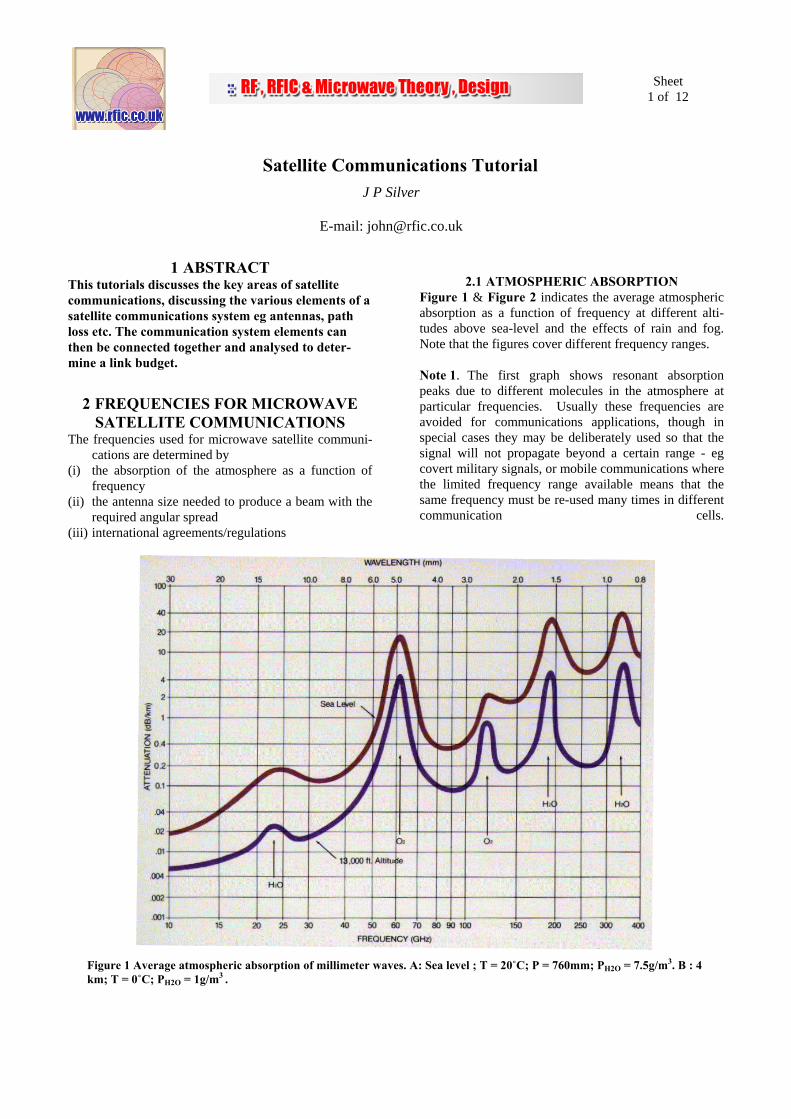
Sheet 1 of 12 Satellite Communications Tutorial J P Silver E-mail: [email protected] 1 ABSTRACT This tutorials discusses the key areas of satellite communications, discussing the various elements of a satellite communications system eg antennas, path loss etc. The communication system elements can then be connected together and analysed to deter- mine a link budget. 2 FREQUENCIES FOR MICROWAVE SATELLITE COMMUNICATIONS The frequencies used for microwave satellite communi- cations are determined by (i) the absorption of the atmosphere as a function of frequency (ii) the antenna size needed to produce a beam with the required angular spread (iii) international agreements/regulations 2.1 ATMOSPHERIC ABSORPTION Figure 1 & Figure 2 indicates the average atmospheric absorption as a function of frequency at different alti- tudes above sea-level and the effects of rain and fog. Note that the figures cover different frequency ranges. Note 1. The first graph shows resonant absorption peaks due to different molecules in the atmosphere at particular frequencies. Usually these frequencies are avoided for communications applications, though in special cases they may be deliberately used so that the signal will not propagate beyond a certain range - eg covert military signals, or mobile communications where the limited frequency range available means that the same frequency must be re-used many times in different communication cells. Figure 1 Average atmospheric absorption of millimeter waves. A: Sea level ; T = 20˚C; P = 760mm; P H2O = 7.5g/m 3 . B : 4 km; T = 0˚C; P H2O = 1g/m 3 .
description
This tutorials discusses the key areas of satellitecommunications, discussing the various elements of asatellite communications system eg antennas, pathloss etc.
Transcript of Satellite Communications
Sheet
1 of 12
Satellite Communications Tutorial J P Silver
E-mail: [email protected]
1 ABSTRACT This tutorials discusses the key areas of satellite communications, discussing the various elements of a satellite communications system eg antennas, path loss etc. The communication system elements can then be connected together and analysed to deter-mine a link budget.
2 FREQUENCIES FOR MICROWAVE SATELLITE COMMUNICATIONS
The frequencies used for microwave satellite communi-cations are determined by
(i) the absorption of the atmosphere as a function of frequency
(ii) the antenna size needed to produce a beam with the required angular spread
(iii) international agreements/regulations
2.1 ATMOSPHERIC ABSORPTION Figure 1 & Figure 2 indicates the average atmospheric absorption as a function of frequency at different alti-tudes above sea-level and the effects of rain and fog. Note that the figures cover different frequency ranges. Note 1. The first graph shows resonant absorption peaks due to different molecules in the atmosphere at particular frequencies. Usually these frequencies are avoided for communications applications, though in special cases they may be deliberately used so that the signal will not propagate beyond a certain range - eg covert military signals, or mobile communications where the limited frequency range available means that the same frequency must be re-used many times in different communication cells.
Figure 1 Average atmospheric absorption of millimeter waves. A: Sea level ; T = 20˚C; P = 760mm; PH2O = 7.5g/m3. B : 4 km; T = 0˚C; PH2O = 1g/m3 .
Sheet
2 of 12
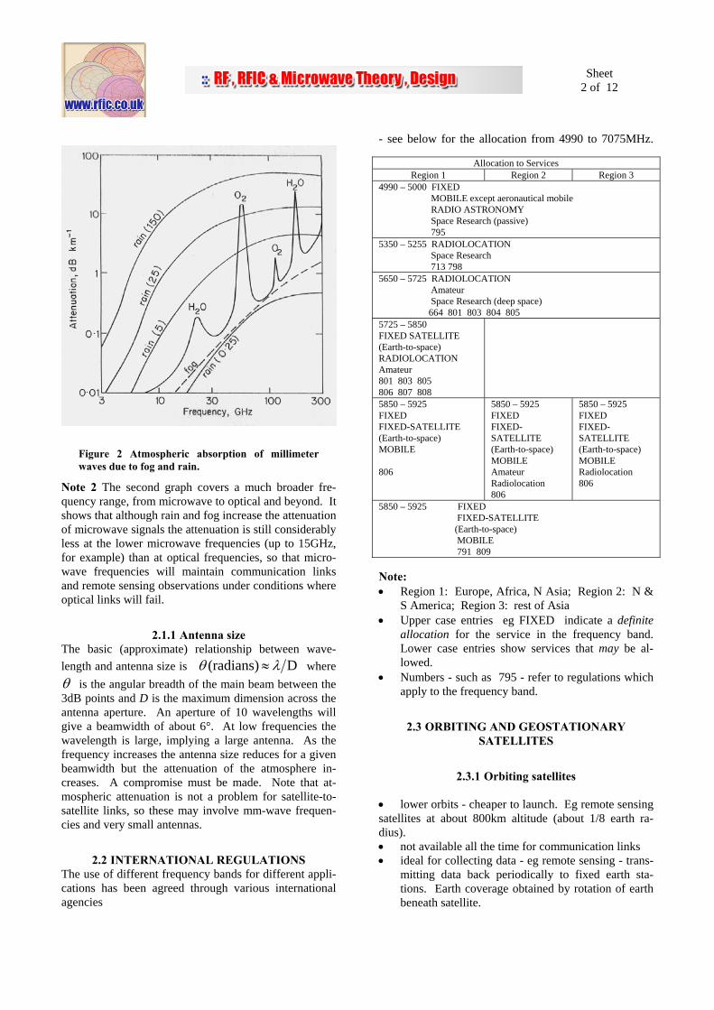
Figure 2 Atmospheric absorption of millimeter waves due to fog and rain.
Note 2 The second graph covers a much broader fre-quency range, from microwave to optical and beyond. It shows that although rain and fog increase the attenuation of microwave signals the attenuation is still considerably less at the lower microwave frequencies (up to 15GHz, for example) than at optical frequencies, so that micro-wave frequencies will maintain communication links and remote sensing observations under conditions where optical links will fail.
2.1.1 Antenna size The basic (approximate) relationship between wave-length and antenna size is D (radians) λθ ≈ where θ is the angular breadth of the main beam between the 3dB points and D is the maximum dimension across the antenna aperture. An aperture of 10 wavelengths will give a beamwidth of about 6°. At low frequencies the wavelength is large, implying a large antenna. As the frequency increases the antenna size reduces for a given beamwidth but the attenuation of the atmosphere in-creases. A compromise must be made. Note that at-mospheric attenuation is not a problem for satellite-to-satellite links, so these may involve mm-wave frequen-cies and very small antennas.
2.2 INTERNATIONAL REGULATIONS The use of different frequency bands for different appli-cations has been agreed through various international agencies
- see below for the allocation from 4990 to 7075MHz.
Allocation to Services Region 1 Region 2 Region 3
4990 – 5000 FIXED MOBILE except aeronautical mobile RADIO ASTRONOMY Space Research (passive) 795 5350 – 5255 RADIOLOCATION Space Research 713 798 5650 – 5725 RADIOLOCATION Amateur Space Research (deep space) 664 801 803 804 805 5725 – 5850 FIXED SATELLITE (Earth-to-space) RADIOLOCATION Amateur 801 803 805 806 807 808
5850 – 5925 FIXED FIXED-SATELLITE (Earth-to-space) MOBILE 806
5850 – 5925 FIXED FIXED-SATELLITE (Earth-to-space) MOBILE Amateur Radiolocation 806
5850 – 5925 FIXED FIXED-SATELLITE (Earth-to-space) MOBILE Radiolocation 806
5850 – 5925 FIXED FIXED-SATELLITE (Earth-to-space) MOBILE 791 809 Note: • Region 1: Europe, Africa, N Asia; Region 2: N &
S America; Region 3: rest of Asia • Upper case entries eg FIXED indicate a definite
allocation for the service in the frequency band. Lower case entries show services that may be al-lowed.
• Numbers - such as 795 - refer to regulations which apply to the frequency band.
2.3 ORBITING AND GEOSTATIONARY SATELLITES
2.3.1 Orbiting satellites • lower orbits - cheaper to launch. Eg remote sensing satellites at about 800km altitude (about 1/8 earth ra-dius). • not available all the time for communication links • ideal for collecting data - eg remote sensing - trans-
mitting data back periodically to fixed earth sta-tions. Earth coverage obtained by rotation of earth beneath satellite.
Sheet
3 of 12
• receive antennas must track satellite • lower coverage than geostationary
2.3.2 Geostationary satellites • occupy fixed position with respect to earth above
the equator - no tracking required • 3 satellites provide coverage for most of earth's sur-
face (not polar regions)
• Data: radius of orbit: 42 000km (about 7 times earth radius) altitude: 36 000km orbital period: 24hours
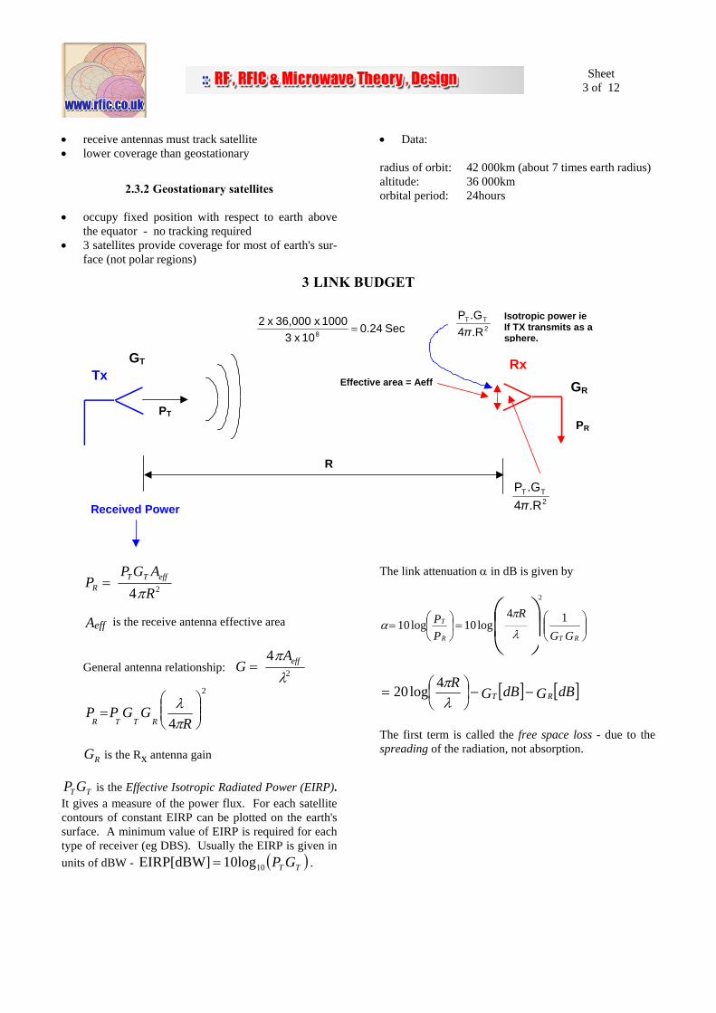
3 LINK BUDGET
Tx GT
PT
R
Rx GR
PR
Effective area = Aeff
2TT
.R4.GPπ
Isotropic power ie If TX transmits as a sphere.
2TT
.R4.GPπSec 0.24
10 x 31000 x 36,000 x 2
8 =
Received Power
PP G A
RRT T eff=4 2π
effA is the receive antenna effective area
General antenna relationship: GAeff=
42
πλ
2
4 ⎟⎟⎠
⎞⎜⎜⎝
⎛=
RGGPP
RTTR πλ
GR is the Rx antenna gain
P GT T is the Effective Isotropic Radiated Power (EIRP). It gives a measure of the power flux. For each satellite contours of constant EIRP can be plotted on the earth's surface. A minimum value of EIRP is required for each type of receiver (eg DBS). Usually the EIRP is given in units of dBW - ( )TT GP1010logEIRP[dBW] = .
The link attenuation α in dB is given by
⎟⎟⎠
⎞⎜⎜⎝
⎛=⎟
⎠
⎞⎜⎝
⎛= ⎟
⎠⎞
⎜⎝⎛
GG
R
PP
RTR
T 14log10log10
2
λ
πα
[ ] [ ]dBGdBGR
RT −−⎟⎠⎞
⎜⎝⎛=λπ4log20
The first term is called the free space loss - due to the spreading of the radiation, not absorption.
Sheet
4 of 12
3.1 DBW (DECIBEL WATTS) Link budget calculations are often carried out using powers measured in dBW. The power is measured rela-tive to a 1 watt reference power. Power in dBW 10 log Power in Watts
1 Watt=
[ ] [ ] [ ] ⎟⎠⎞
⎜⎝⎛−+=λπR
GEIRPP RR4log20dBdBWdBW
Corrections must be added to RP for additional losses due to 1. antenna efficiency - power is lost in the antenna
feed structure, also in connections to the receiver 2. atmospheric absorption due to water and oxygen
molecules 3. polarisation mismatches of Tx and Rx antennas 4. antenna misalignments - ie boresights of Tx and
Rx antennas not aligned An additional loss factor L is introduced to the link budget equation to take account of these losses. The equations become
( ) LRGGPP RTTR
14
2
πλ=
[ ] [ ] [ ] [ ] ( ) [ ]dB4log20dBdBdBWdBW LRGGPP RTTR −−++=
λπ
Typically L is about 5dB.
3.2 LINK BUDGET CALCULATION Calculate the power that must be transmitted from a geo-stationary satellite to give a power of -116dBW (2.5 × 10⁻²¹ W) at a receiver on the earth. Assume f=10GHz,
dB40=RG , dB30=TG and additional losses of 5dB. R = altitude = 36000km
[ ] [ ] [ ] [ ] ( ) [ ]dB4log20dBdBdBWdBW LRGGPP RTTR −−++=
λπ
[ ] [ ] 52034030dBWdBW116 −−++=−
TP
∴ =TP dBW dBW = 159W22 and EIRP = 22 dBW + 30dB = 52 dBW
3.3 ANTENNA BEAMWIDTH AND GAIN The satellite antenna beamwidth must correspond to the area of the earth to be illuminated. This determines the gain of the antenna. The earth station antenna must be able to select a particular geostationary satellite - the satellite spacing in the crowded parts of the geostation-ary orbit is about 2°, though there may also be frequency discrimination between neighbouring satellites. The following approximate results for a circular aperture antenna may be used to estimate suitable antenna sizes and gains.
( )λπη DG
2
=
η is the antenna efficiency, typically 0.6 to 0.7, D is the antenna diameter θ λ3 70dB = D the 3dB beamwidth in degrees of the antenna.
3.4 SYSTEM NOISE TEMPERATURE For satisfactory operation a communication link must have: 1. a large enough signal for the receiver sensitivity,
and 2. a high enough S/N ratio or BER at the receiver
output for good quality communication eg for TV reception international regulations re-
quire a S/N ratio ≥ 47dB Information is conveyed by modulating a high frequency carrier with a message signal. The basic quality of a link is expressed in terms of its carrier to noise ratio C/N where C is the power for the unmodulated carrier and N is the noise power, both measured at the receiver input. The signal to noise ratio for an information signal - ie a modulated carrier - depends upon both the C/N ratio for the link and the type of modulation used - ie AM, FM, FSK, PSK etc.
Sheet
5 of 12
The noise power associated with the link is specified by the system noise temperature Ts. This is made up from three contributions:
1. antenna noise TA 2. antenna - receiver connection - a cable or waveguide TC 3. receiver noise TR this may include RF, mixer and IF stage contributions
In each case the noise power in watts (this is the avail-able noise power) is calculated from the noise tempera-
ture (which must be in degrees K, ie absolute tempera-ture) using the general relationship available noise power = kTB where k is Boltzmann's constant and B is the bandwidth. k = 1.38 × 10⁻²³ J K-1
A useful figure to remember is that at 290K the available noise power density is -174dBm/Hz
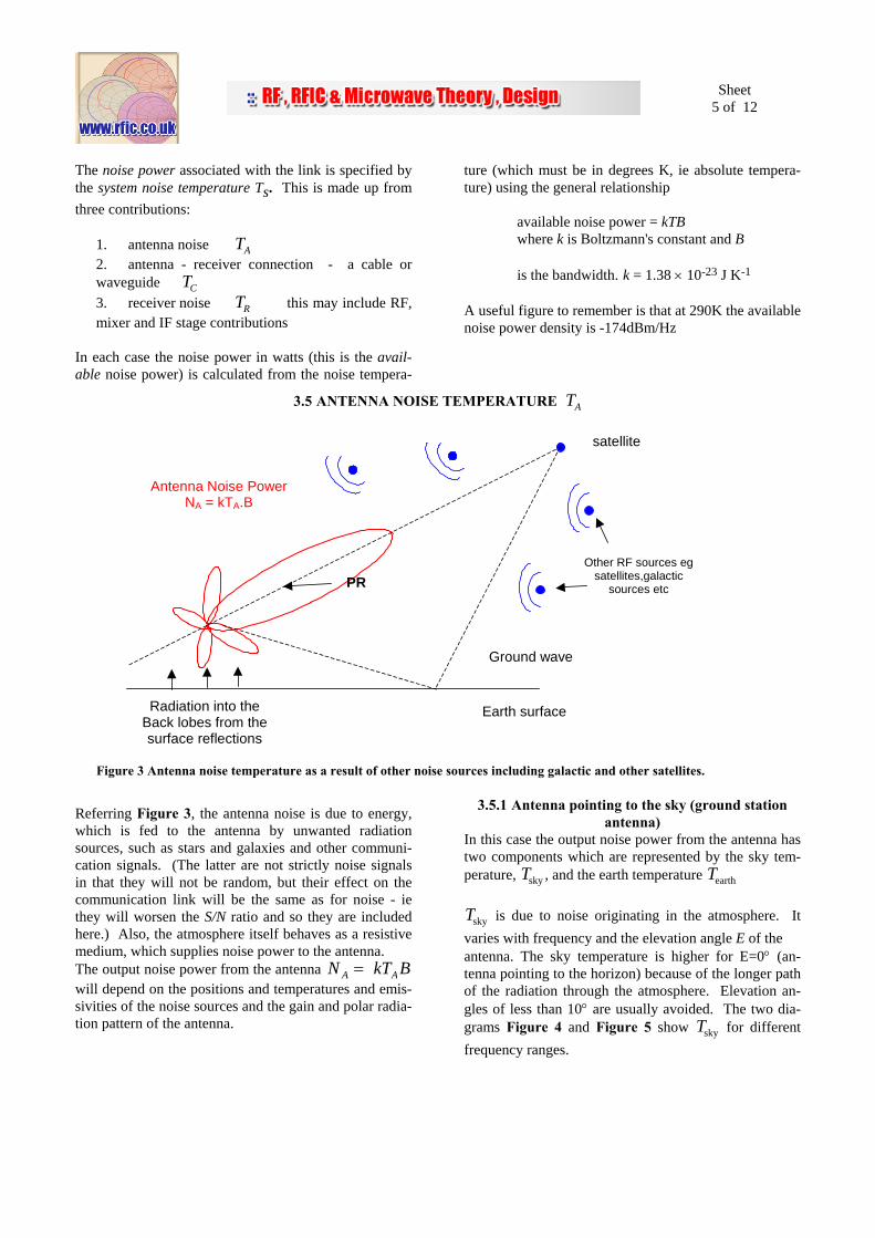
3.5 ANTENNA NOISE TEMPERATURE TA
PR
Radiation into the Back lobes from the surface reflections
Ground wave
Other RF sources eg satellites,galactic
sources etc
satellite
Antenna Noise Power NA = kTA.B
Earth surface
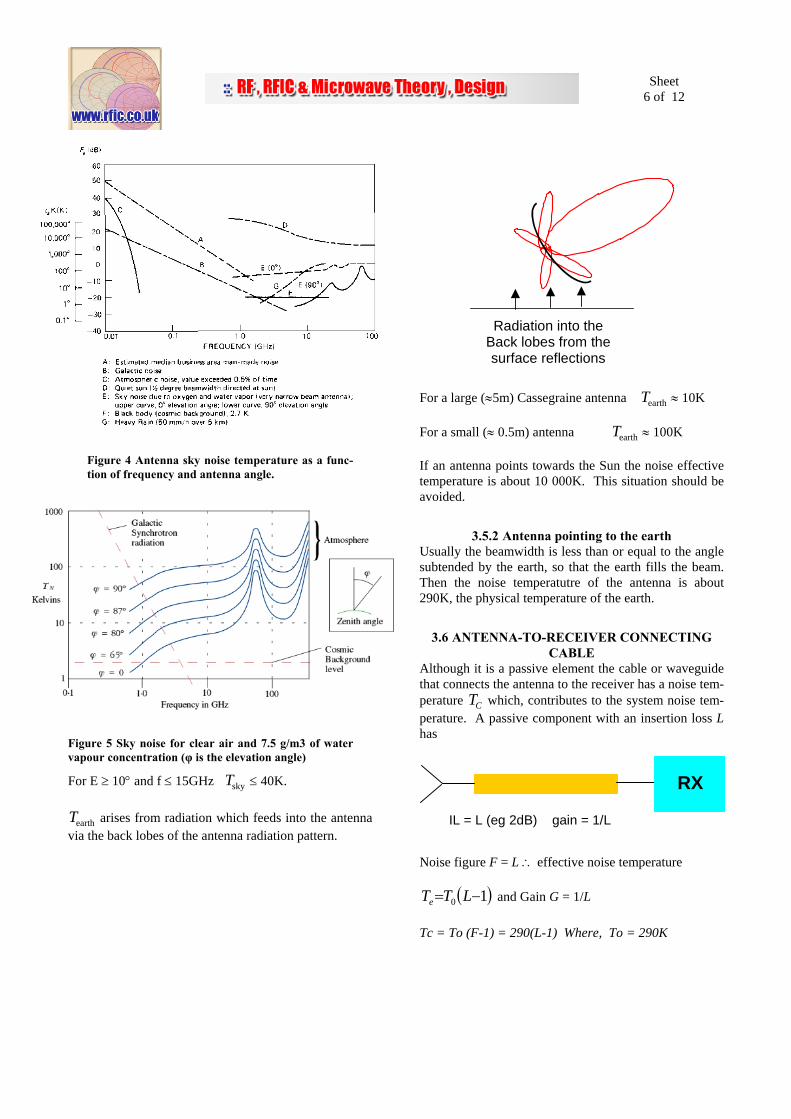
Figure 3 Antenna noise temperature as a result of other noise sources including galactic and other satellites.
Referring Figure 3, the antenna noise is due to energy, which is fed to the antenna by unwanted radiation sources, such as stars and galaxies and other communi-cation signals. (The latter are not strictly noise signals in that they will not be random, but their effect on the communication link will be the same as for noise - ie they will worsen the S/N ratio and so they are included here.) Also, the atmosphere itself behaves as a resistive medium, which supplies noise power to the antenna. The output noise power from the antenna N kT BA A= will depend on the positions and temperatures and emis-sivities of the noise sources and the gain and polar radia-tion pattern of the antenna.
3.5.1 Antenna pointing to the sky (ground station antenna)
In this case the output noise power from the antenna has two components which are represented by the sky tem-perature, Tsky , and the earth temperature Tearth Tsky is due to noise originating in the atmosphere. It varies with frequency and the elevation angle E of the antenna. The sky temperature is higher for E=0° (an-tenna pointing to the horizon) because of the longer path of the radiation through the atmosphere. Elevation an-gles of less than 10° are usually avoided. The two dia-grams Figure 4 and Figure 5 show Tsky for different frequency ranges.
Sheet
6 of 12
Figure 4 Antenna sky noise temperature as a func-tion of frequency and antenna angle.
Figure 5 Sky noise for clear air and 7.5 g/m3 of water vapour concentration (φ is the elevation angle)
For E ≥ 10° and f ≤ 15GHz Tsky ≤ 40K. Tearth arises from radiation which feeds into the antenna via the back lobes of the antenna radiation pattern.
Radiation into the Back lobes from the surface reflections
For a large (≈5m) Cassegraine antenna Tearth ≈ 10K For a small (≈ 0.5m) antenna Tearth ≈ 100K If an antenna points towards the Sun the noise effective temperature is about 10 000K. This situation should be avoided.
3.5.2 Antenna pointing to the earth Usually the beamwidth is less than or equal to the angle subtended by the earth, so that the earth fills the beam. Then the noise temperatutre of the antenna is about 290K, the physical temperature of the earth.
3.6 ANTENNA-TO-RECEIVER CONNECTING CABLE
Although it is a passive element the cable or waveguide that connects the antenna to the receiver has a noise tem-perature TC which, contributes to the system noise tem-perature. A passive component with an insertion loss L has
RX
IL = L (eg 2dB) gain = 1/L
Noise figure F = L ∴ effective noise temperature
( )10 −= LTTe and Gain G = 1/L Tc = To (F-1) = 290(L-1) Where, To = 290K
Sheet
7 of 12
3.7 RECEIVER NOISE
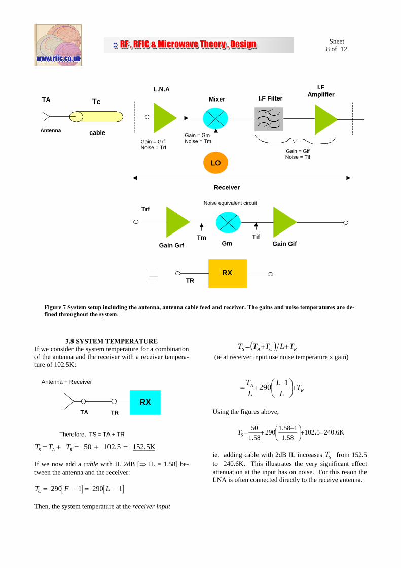
Receiver noise includes contributions from thermal noise, shot noise and possibly flicker noise. These may arise in the input RF section of the receiver, the mixers used for frequency translation and the IF stages. A schematic diagram of a simple receiver and its equiva-lent noise circuit is shown below. The total receiver noise figure RT can be calculated from the individual contributions from the usual formula for cascaded cir-cuits.
( )1−= RoR FTT FR is the receiver noise figure In the schematic receiver shown in Figure 7.
mrf
if
rf
mrfR GG
TGT
TT ++=
Note: This formula follows from the corresponding for-mula for the noise figure Ftotal for cascaded stages,
...11
21
3
1
21total +
−+
−+=
GGF
GF
FF with
each noise figure replaced by its equivalent effective noise temperature using ( )1−= FTT oe . Example LNA (low noise amplifier) T G Grf rf rf= =50 23K dB [ = 200] Mixer T G Gm m m= = =500 0K dB [ 1] IF stage T G GIF IF IF= = =1000 30K dB [ 1000]
∴ = + +×
= + + =TR 50 500200
1000200 1
50 2 5 5 57 5. . K
Usually, the mixer has conversion loss eg suppose dBG Gm m=− ∴ =+10 0 1.
∴ = + +×
= + + =T KR 50 500200
1000200 0 1
50 2 5 50 102 5.
. .
mrf
if
rf
mrfR GG
TGT
TT ++=
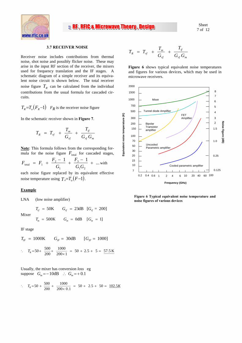
Figure 6 shows typical equivalent noise temperatures and figures for various devices, which may be used in microwave receivers.
15
20
30
50
70
100
150
200
300
500
700
1000
1500
2000
0.2
10
7
1.5
0.125
1.0
0.25
2
3
4
5
6
7
8
0.60.4 2 1 6 4 20 10 10040 60
Frequency (GHz)
Equi
vale
nt n
oise
tem
pera
ture
(K)
Noise figure (dB
)
Mixer
Tunnel diode Amplifier
Cooled parametric amplifier
FET Amplifier
Uncooled Parametric amplifier
Bipolar Transistor amplifier
Figure 6 Typical equivalent noise temperature and noise figures of various devices
Sheet
8 of 12
LO
Receiver
Tc
cable
TA
Antenna
L.N.AMixer I.F Filter
I.F Amplifier
Gain = Gif Noise = Tif
Gain = Gm Noise = Tm Gain = Grf
Noise = Trf
Noise equivalent circuit Trf
Gain Grf Gm Tm
Gain Gif Tif
RXTR
___ ___ ___
Figure 7 System setup including the antenna, antenna cable feed and receiver. The gains and noise temperatures are de-fined throughout the system.
3.8 SYSTEM TEMPERATURE If we consider the system temperature for a combination of the antenna and the receiver with a receiver tempera-ture of 102.5K:
RX
Antenna + Receiver
TA TR
Therefore, TS = TA + TR
T T TS A R= + = + =50 102 5 152 5. . K If we now add a cable with IL 2dB [⇒ IL = 1.58] be-tween the antenna and the receiver: T F LC = − = −290 1 290 1 Then, the system temperature at the receiver input
( ) RCAS TLTTT ++= (ie at receiver input use noise temperature x gain)
RA T
LL
LT
+⎟⎠⎞
⎜⎝⎛ −
+=1290
Using the figures above,
K6.2405102581
1581290581
50=+⎟
⎠⎞
⎜⎝⎛ −
+= ..
..ST
ie. adding cable with 2dB IL increases TS from 152.5 to 240.6K. This illustrates the very significant effect attenuation at the input has on noise. For this reaon the LNA is often connected directly to the receive antenna.
Sheet
9 of 12
3.9 C/N RATIO AT RECEIVER OUTPUT
Tx GT
PT
R
Rx GR
PR
L1.
R.4.).GGP(
2
RTT ⎟⎠⎞
⎜⎝⎛+=πλ
˜ C = Carrier power
From before: ( )LR
GGPP RTTR1
4
2
⎟⎠⎞
⎜⎝⎛=πλ
If system temperature is TS (includes antenna noise TA , cable and receiver noise) Noise power (single link) at receiver input is
N kT BS=
( )kBLRT
GGPBkTP
NC
s
RTT
s
R 114
link2
⎟⎠⎞
⎜⎝⎛
⎟⎟⎠
⎞⎜⎜⎝
⎛==∴
πλ
merit.offigurereceiver theis ⎟⎟⎠
⎞⎜⎜⎝
⎛
S
R
TG
Usually the down link is the most critical due to the lim-ited power which is available on board the satellite ( PT ) and the antenna gain GT (limited by its size). Hence, the most critical receiver is the earth station eg Intelstat ground station
GHz 4at 740 1−=⎟⎟⎠
⎞⎜⎜⎝
⎛dBK
TG
S
R .
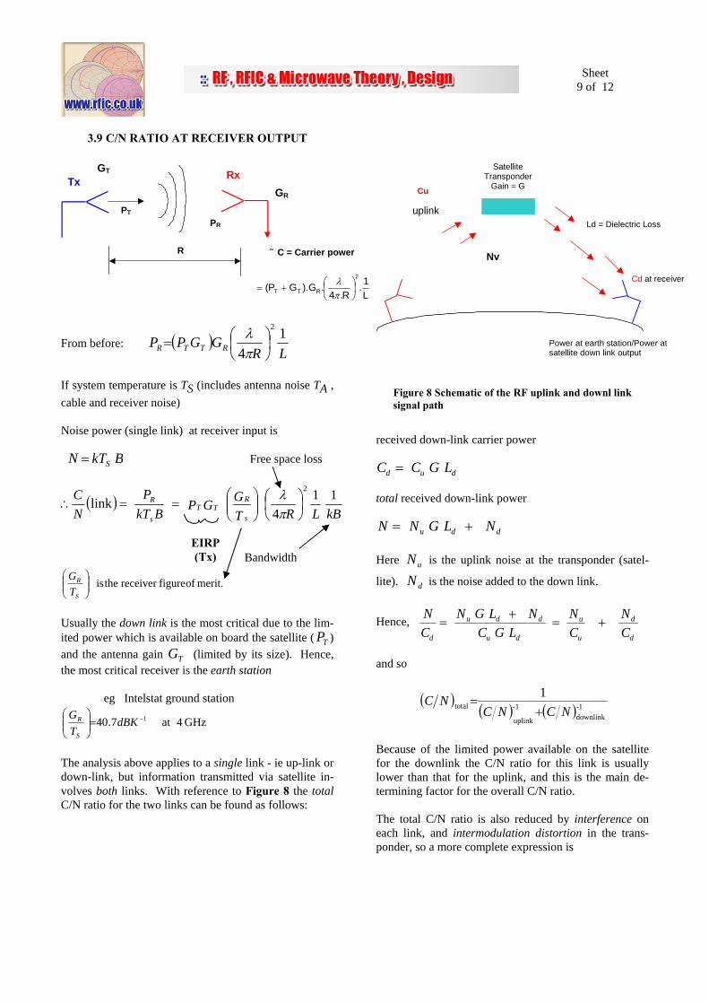
The analysis above applies to a single link - ie up-link or down-link, but information transmitted via satellite in-volves both links. With reference to Figure 8 the total C/N ratio for the two links can be found as follows:
Satellite
Transponder Gain = G
Ld = Dielectric Loss uplink
Nv
Cd at receiver
Power at earth station/Power at satellite down link output
Cu
Figure 8 Schematic of the RF uplink and downl link signal path
received down-link carrier power C C G Ld u d= total received down-link power N N G L Nu d d= + Here uN is the uplink noise at the transponder (satel-
lite). dN is the noise added to the down link.
Hence, NC
N G L NC G L
NC
NCd
u d d
u d
u
u
d
d
=+
= +
and so
( )( ) ( ) 1-
downlink1-
uplink
total1
NCNCNC
+=
Because of the limited power available on the satellite for the downlink the C/N ratio for this link is usually lower than that for the uplink, and this is the main de-termining factor for the overall C/N ratio. The total C/N ratio is also reduced by interference on each link, and intermodulation distortion in the trans-ponder, so a more complete expression is
EIRP (Tx)
Free space loss
Bandwidth
Sheet
10 of 12
( )( ) ( ) ( ) ( ) ( ) 1
intermods1-downlink
1-
uplink
1-downlink
1-
uplink
total1
−++++=
NCICICNCNCNC
Calculations using the above relationships apply to clear air propagation conditions, but allowance has to be made for additional attenuation and noise which may be introduced on each link due to rainfall or other possible meteorological conditions. The margin that must be allowed depends upon the required reliability (eg link maintained for 99.99% of time, averaged over one year) and the range of climatic conditions which are predicted along the link. The margins also vary with frequency and the angle of elevation. Typical margin values are 2dB (C band) and 8dB (Ku band).
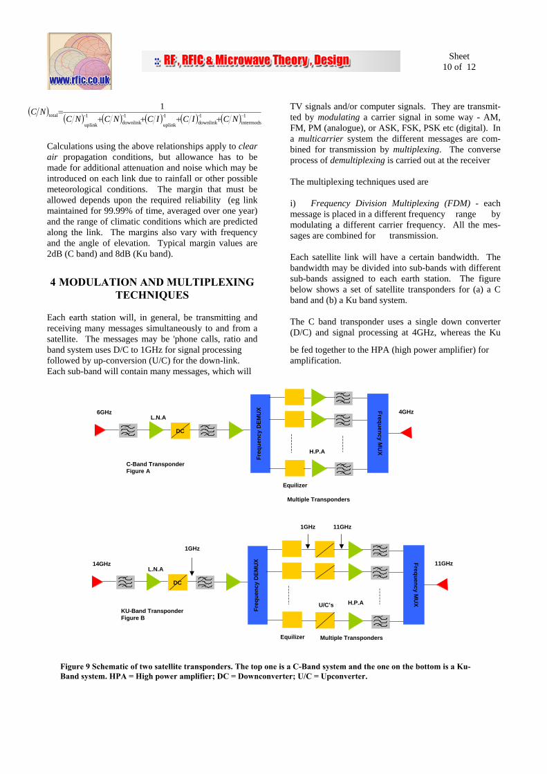
4 MODULATION AND MULTIPLEXING TECHNIQUES
Each earth station will, in general, be transmitting and receiving many messages simultaneously to and from a satellite. The messages may be 'phone calls, ratio and
TV signals and/or computer signals. They are transmit-ted by modulating a carrier signal in some way - AM, FM, PM (analogue), or ASK, FSK, PSK etc (digital). In a multicarrier system the different messages are com-bined for transmission by multiplexing. The converse process of demultiplexing is carried out at the receiver The multiplexing techniques used are i) Frequency Division Multiplexing (FDM) - each message is placed in a different frequency range by modulating a different carrier frequency. All the mes-sages are combined for transmission. Each satellite link will have a certain bandwidth. The bandwidth may be divided into sub-bands with different sub-bands assigned to each earth station. The figure below shows a set of satellite transponders for (a) a C band and (b) a Ku band system. The C band transponder uses a single down converter (D/C) and signal processing at 4GHz, whereas the Ku
band system uses D/C to 1GHz for signal processing followed by up-conversion (U/C) for the down-link. Each sub-band will contain many messages, which will
be fed together to the HPA (high power amplifier) for amplification.
6GHz
DC
L.N.A
Multiple Transponders
Freq
uenc
y D
EMU
X
Equilizer
H.P.A
Frequency MU
X
4GHz
14GHz
DC
L.N.A
Multiple Transponders
Freq
uenc
y D
EMU
X
Equilizer
H.P.A
Frequency MU
X
11GHz
1GHz
U/C’s
1GHz 11GHz
C-Band Transponder Figure A
KU-Band Transponder Figure B
Figure 9 Schematic of two satellite transponders. The top one is a C-Band system and the one on the bottom is a Ku-Band system. HPA = High power amplifier; DC = Downconverter; U/C = Upconverter.
Sheet
11 of 12
In the C band 6/4GHz transponder (Figure 9 A): • the uplink is at the higher frequency, so λD is
greater for the (common) receive/transmit antenna – it will have a higher gain
• the input filter is a fairly wideband band-pass‘roofing’ filter to allow all the uplink frequen-cies in, but eliminating out-of-band noise
• LNA – low noise amplifier • D/C – down converter to 4GHz (the down-link fre-
quency) for signal processing – error correction, amplification, signal channelling etc.
• frequency demultiplexing – divides input signal into sub-bands to reduce non-linear distortion during amplification. Each sub-frequency band is proc-essed by a single transponder.
• equalisers – correct for phase differences between the different frequency components of a signal which are introduced by filters, de-multiplexers etc
• HPAs – high power amplifiers – to increase power levels before re-transmission on the down-link. Non-linear performance in the HPAs can intoduce harmonics, intermodulation distortion etc
• band-pass filters at various points remove out-of-band products from the HPAs etc and reduce the background noise, but they cannot remove in-band products – eg 3rd order intermodulation (IM) prod-ucts
The Ku (14/11GHz) system (Figure 9 – B) has many of the same elements, but the down-link frequency (11GHz) is too high for the elements in each trans-ponder, so the input is mixed down from 14GHz to 1GHz for de-multiplexing and equalisation, then mixed up to 11GHz for power amplification, frequency MUX and re-transmission.
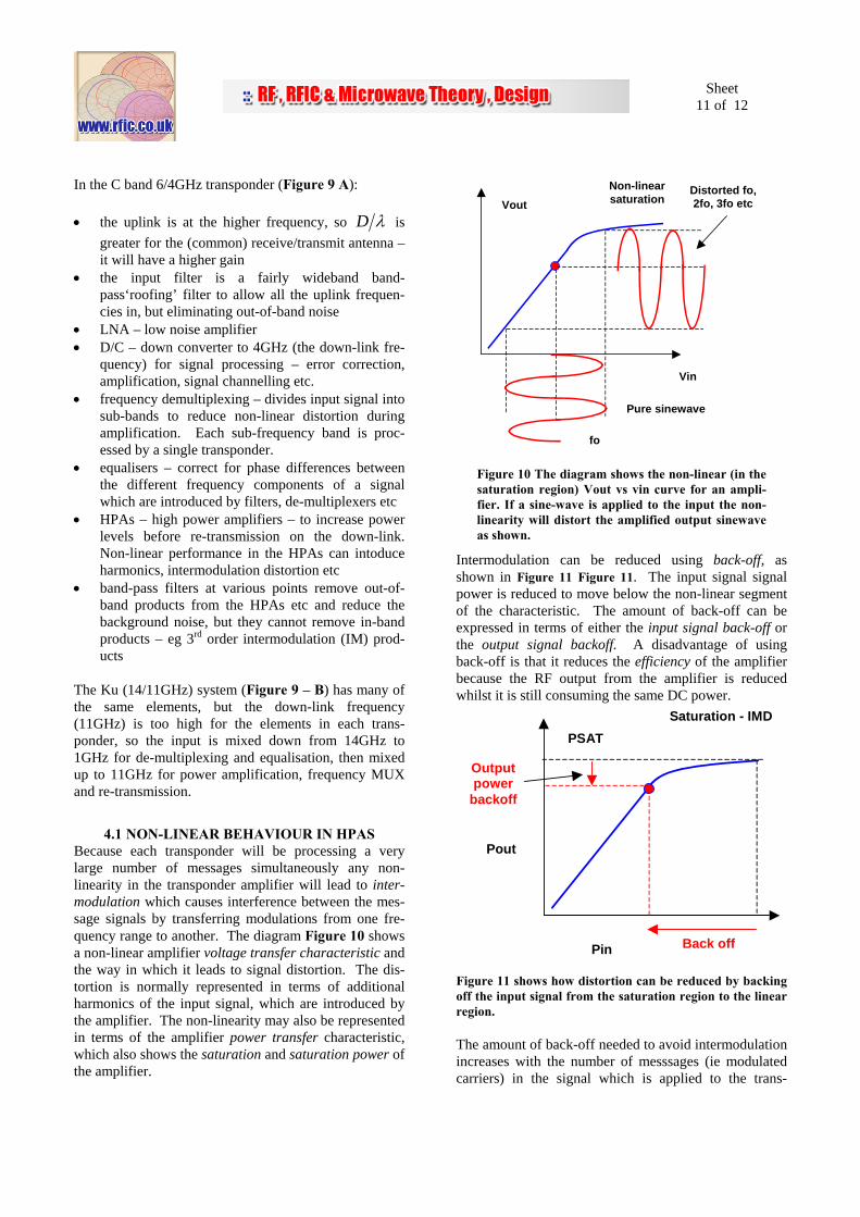
4.1 NON-LINEAR BEHAVIOUR IN HPAS Because each transponder will be processing a very large number of messages simultaneously any non-linearity in the transponder amplifier will lead to inter-modulation which causes interference between the mes-sage signals by transferring modulations from one fre-quency range to another. The diagram Figure 10 shows a non-linear amplifier voltage transfer characteristic and the way in which it leads to signal distortion. The dis-tortion is normally represented in terms of additional harmonics of the input signal, which are introduced by the amplifier. The non-linearity may also be represented in terms of the amplifier power transfer characteristic, which also shows the saturation and saturation power of the amplifier.
Vout
Pure sinewave
Vin
Non-linear saturation
Distorted fo, 2fo, 3fo etc
fo
Figure 10 The diagram shows the non-linear (in the saturation region) Vout vs vin curve for an ampli-fier. If a sine-wave is applied to the input the non-linearity will distort the amplified output sinewave as shown.
Intermodulation can be reduced using back-off, as shown in Figure 11 Figure 11. The input signal signal power is reduced to move below the non-linear segment of the characteristic. The amount of back-off can be expressed in terms of either the input signal back-off or the output signal backoff. A disadvantage of using back-off is that it reduces the efficiency of the amplifier because the RF output from the amplifier is reduced whilst it is still consuming the same DC power.
Pout
Back off Pin
Saturation - IMDPSAT
Output power
backoff
Figure 11 shows how distortion can be reduced by backing off the input signal from the saturation region to the linear region. The amount of back-off needed to avoid intermodulation increases with the number of messsages (ie modulated carriers) in the signal which is applied to the trans-
Sheet
12 of 12
ponder. One solution is to increase the number of trans-ponders on board the satellite so that each need only handle a restricted bandwidth and number of carriers. This, of course, increases the satellite mass, so a suitable compromise must be reached between the number of transponders and the intermodulation. Back-off modifies the formula for the down-link C/N ratio by making : P P BOT os o= − Where, Pos is the output power of the HPA at satura-tion and BOo is the output backoff power . Pos is normally known for a given amplifier, then oBO is adjusted dynamically according to the strength of the input signal. Solid state amplifiers are superior to TWT amplifiers in their linearity. Considerable attention has been devoted to techniques for linearising HPAs to improve their effi-ciency. This involves extending the linear part of the power amplifier characteristic. ii) Time Division Multiplexing (TDM) - each message is transmitted at a different time. TDM is usually used with digitally coded messages. Whereas with FDM each message is transmitted continuously using a restricted bandwidth, with TDM each message is only transmitted for a small fraction of the available time, but during that time it uses all the available bandwidth. Clearly, a system must be established to regulate the timeslots for each message. This scheduling will itself require the communication of earth stations via the satel-lite which imposes a network management overhead on the available bandwidth/transmission time. An appro-priate balance must be struck between the complexity of the 'housekeeping' of the communication system and the useful communication capacity. An advantage of TDM is that intermodulation distortion can be avoided, because only one message is being am-plified at any one time. iii) Code Division Multiplex (CDM) - each message includes a unique code which means that TDMA can be used with different signals being transmitted simultane-ously - the code allows the elements of the different messages to be grouped correctly. CDM uses a very wide bandwidth and so this technique is sometimes also known as a spread spectrum technique.
4.2 MULTIPLE ACCESS Multiple access refers to the fact that many earth stations share the same satellite. Signals from several earth sta-
tions may arrive simultaneously at the satellite antenna from which they are fed to the transponder which will process the signals in several ways - eg amplification, error detection and correction, filtering and frequency changing - before feeding the signals back to the satellite antenna for the down link. The uplink and the down link operate at different frequencies to avoid direct cou-pling of signals from the transmit to the receive channels eg 6/4GHz (C band), 14/11GHz Ku band). The higher frequency is used for the up-link because the satellite antenna has limited size and a higher noise temperature (usually 290K). The gain is higher at the upper fre-quency for a fixed antenna size. Similarly, the signals transmitted from a satellite will usually be received by all the earth stations. Most of the messages received will not be needed by a specific earth station - they must be filtered out during de-multiplexing. In a typical analogue system a trans-ponder may have a bandwidth of 36MHz, but this will be subdivided into 12 sub-bands, each with a bandwidth of 3MHz. When an earth station receives messages from its vicinity via the PSTN network it sorts them out into their destination earth stations. All the messages for a particular earth station are combined to one sub-band for the uplink. They are all processed by the satellite transponder and transmitted to the earth stations, but each earth station will only process its own sub-band. As noted earlier, multiplexing and modulation are sepa-rate processes and so various combinations of the differ-ent techniques available for each can be used. Accord-ing to Glover and Grant, the predominant multiplex-ing/modulation/multiple access technique in current use for PSTN satellite telephony is FDM/FM/FDMA, but this leads to large intermodulation products. Increas-ingly, digital modulation (PCM) is replacing analogue techniques, leading to TDM/PSK/TDMA. With the systems described so far the communication capacity between different earth stations is essentially 'designed in' when the bandwidths assigned to each sta-tion are fixed, and changes cannot easily be made even if demand changes. Capacity can be increased, and made more flexible, by i) using multiple spot beams that can be steered as required to different points on the earth's surface, and ii) by using a switching matrix on board the satellite to co-ordinate the message transmission with the beam direction.
![Satellite communications[1]](https://static.fdocuments.in/doc/165x107/588ae6481a28abab6c8b6391/satellite-communications1.jpg)