
Satellite Communication...
269
Transcript of Satellite Communication...
Marcel Dekker, Inc. New York • BaselTM
Satellite Communication
Engineering
Michael O. KolawoleJolade Pty. Ltd.
Melbourne, Australia
Copyright © 2002 by Marcel Dekker, Inc. All Rights Reserved.

ISBN: 0-8247-0777-X
This book is printed on acid-free paper.
Headquarters
Marcel Dekker, Inc.
270 Madison Avenue, New York, NY 10016
tel: 212-696-9000; fax: 212-685-4540
Eastern Hemisphere Distribution
Marcel Dekker AG
Hutgasse 4, Postfach 812, CH-4001 Basel, Switzerland
tel: 41-61-261-8482; fax: 41-61-261-8896
World Wide Web
http://www.dekker.com
The publisher offers discounts on this book when ordered in bulk quantities. For more
information, write to Special Sales=Professional Marketing at the headquarters address
above.
Copyright # 2002 by Marcel Dekker, Inc. All Rights Reserved.
Neither this book nor any part may be reproduced or transmitted in any form or by any
means, electronic or mechanical, including photocopying, microfilming, and recording,
or by any information storage and retrieval system, without permission in writing from
the publisher.
Current printing (last digit):
10 9 8 7 6 5 4 3 2 1
PRINTED IN THE UNITED STATES OF AMERICA
Copyright © 2002 by Marcel Dekker, Inc. All Rights Reserved.

This book is dedicated to my families in Australia and Nigeria
for their belief in and support for me.
The joy of family is divine.
For this I am eternally blessed and grateful.
Copyright © 2002 by Marcel Dekker, Inc. All Rights Reserved.
Series Introduction
Over the past 50 years, digital signal processing has evolved as a major
engineering discipline. The fields of signal processing have grown from the
origin of fast Fourier transform and digital filter design to statistical spectral
analysis and array processing, image, audio, and multimedia processing, and
shaped developments in high-performance VLSI signal processor design.
Indeed, there are few fields that enjoy so many applications—signal processing
is everywhere in our lives.
When one uses a cellular phone, the voice is compressed, coded, and
modulated using signal processing techniques. As a cruise missile winds along
hillsides searching for the target, the signal processor is busy processing the
images taken along the way. When we are watching a movie in HDTV, millions
of audio and video data ar being sent to our homes and received with
unbelievable fidelity. When scientists compare DNA samples, fast pattern
recognition techniques are being used. On and on, one can see the impact of
signal processing in almost every engineering and scientific discipline.
Copyright © 2002 by Marcel Dekker, Inc. All Rights Reserved.
Because of the immense importance of signal processing and the fast-
growing demands of business and industry, this series on signal processing
serves to report up-to-date developments and advances in the field. The topics
of interest include but are not limited to the following.
� Signal theory and analysis
� Statistical signal processing
� Speech and audio processing
� Image and video processing
� Multimedia signal processing and technology
� Signal processing for communications
� Signal processing architectures and VLSI design
I hope this series will provide the interested audience with high-quality, state-
of-the-art signal processing literature through research monographs, edited
books, and rigorously written textbooks by experts in their fields.
K. J. Ray Liu
Copyright © 2002 by Marcel Dekker, Inc. All Rights Reserved.
Preface
Satellite communication is one of the most impressive spin-offs from space
programs, and has made a major contribution to the pattern of international
communications. The engineering aspect of satellite communications
combines such diverse topics as antennas, radio wave propagation, signal
processing, data communication, modulation, detection, coding, filtering,
orbital mechanics, and electronics. Each is a major field of study and each
has its own extensive literature. Satellite Communication Engineering empha-
sizes the relevant material from these areas that is important to the book’s
subject matter and derives equations that the reader can follow and understand.
The aim of this book is to present in a simple and concise manner the
fundamental principles common to the majority of information communica-
tions systems. Mastering the basic principles permits moving on to concrete
realizations without great difficulty. Throughout, concepts are developed
mostly on an intuitive, physical basis, with further insight provided by
Copyright © 2002 by Marcel Dekker, Inc. All Rights Reserved.
means of a combination of applications and performance curves. Problem sets
are provided for those seeking additional training. Starred sections containing
basic mathematical development may be skipped with no loss of continuity by
those seeking only a qualitative understanding. The book is intended for
electrical, electronics, and communication engineering students, as well as
practicing engineers wishing to familiarize themselves with the broad field of
information transmission, particularly satellite communications.
The first of the book’s eight chapters covers the basic principles of
satellite communications, including message security (cryptology).
Chapter 2 discusses the technical fundamentals for satellite communica-
tions services, which do not change as rapidly as technology and provides the
reader with the tools necessary for calculation of basic orbit characteristics
such as period, dwell time, and coverage area; antenna system specifications
such as type, size, beam width, and aperture-frequency product; and power
system design. The system building blocks comprising satellite transponder
and system design procedure are also described. While acknowledging that
systems engineering is a discipline on its own, it is my belief that the reader
will gain a broad understanding of system engineering design procedure,
accumulated from my experience in large, complex turnkey projects.
Earth station, which forms the vital part of the overall satellite system, is
the central theme of Chapter 3. The basic intent of data transmission is to
provide quality transfer of information from the source to the receiver with
minimum error due to noise in the transmission channel. To ensure quality
information requires smart signal processing technique (modulation) and
efficient use of system bandwidth (coding, discussed extensively in Chapter
6). The most popular forms of modulation employed in digital communica-
tions, such as BPSK, QPSK, OQPSK, and 8-PSK, are discussed together with
their performance criteria (BER). An overview of information theory is given
to enhance the reader’s understanding of how maximum data can be trans-
mitted reliably over the communication medium. Chapter 3 concludes by
describing a method for calculating system noise temperature and the items
that facilitate primary terrestrial links to and from the Earth stations.
Chapter 4 discusses the process of designing and calculating the carrier-
to-noise ratio as a measure of the system performance standard. The quality of
signals received by the satellite transponder and that retransmitted and
received by the receiving earth station is important if successful information
transfer via the satellite is to be achieved. Within constraints of transmitter
power and information channel bandwidth, a communication system must be
designed to meet certain minimum performance standards. The most impor-
tant performance standard is ratio of the energy bit per noise density in the
Copyright © 2002 by Marcel Dekker, Inc. All Rights Reserved.
information channel, which carries the signals in a format in which they are
delivered to the end users.
To broadcast video, data, and=or audio signals over a wide area to many
users, a single transmission to the satellite is repeated and received by multiple
receivers. While this might be a common application of satellites, there are
others which may attempt to exploit the unique capacity of a satellite medium
to create an instant network and connectivity between any points within its
view. To exploit this geometric advantage, it is necessary to create a system of
multiple accesses in which many transmitters can use the same satellite
transponder simultaneously. Chapter 5 discusses the sharing techniques
called multiple access. Sharing can be in many formats, such as sharing the
transponder bandwidth in separate frequency slots (FDMA), sharing the
transponder availability in time slots (TDMA), or allowing coded signals to
overlap in time and frequency (CDMA). The relative performance of these
sharing techniques is discussed.
Chapter 6 explores the use of error-correcting codes in a noisy commu-
nication environment, and how transmission error can be detected and
correction effected using the forward error correction (FEC) methods,
namely, the linear block and convolutional coding techniques. Examples are
sparingly used as illustrative tools to explain the FEC techniques.
The regulation that covers satellite networks occurs on three levels:
international, regional, and national. Chapter 7 discusses the interaction
among these three regulatory levels.
Customer’s demands for personalized services and mobility, as well as
provision of standardized system solutions, have caused the proliferation of
telecommunications systems. Chapter 8 examines basic mobile-satellite-
system services and their interaction with land-based backbone networks—in
particular the integrated service digital network (ISDN). Since the services
covered by ISDN should also, in principle, be provided by digital satellite
network, it is necessary to discuss in some detail the basic architecture of
ISDN as well as its principal functional groups in terms of reference
configurations, applications, and protocols. Chapter 8 concludes by briefly
looking at cellular mobile system, including cell assignment and internetwork-
ing principles, as well as technological obstacles to providing efficient Internet
access over satellite links.
The inspiration for writing Satellite Communication Engineering comes
partly from my students who have wanted me to share the wealth of my
experience acquired over the years and to ease their burden in understanding
the fundamental principles of satellite communications. A very special thanks
go to my darling wife, Dr. Marjorie Helen Kolawole, who actively reminds me
Copyright © 2002 by Marcel Dekker, Inc. All Rights Reserved.

about my promise to my students, and more importantly to transfer knowledge
to a wider audience. I am eternally grateful for their vision and support.
I also thank Professor Patrick Leung of Victoria University, Melbourne,
Australia, for his review of the manuscript and his constructive criticisms, and
acknowledge the anonymous reviewers for their helpful comments.
Finally, I want to thank my family for sparing me the time, which I
would have otherwise spent with them, and their unconditional love that keeps
me going.
Michael O. Kolawole
Copyright © 2002 by Marcel Dekker, Inc. All Rights Reserved.
Contents
Series Introduction K. J. Ray Liu
Preface
1. Basic Principles of Satellite Communications
1.1 The Origin of Satellites
1.2 Communications Via Satellite
1.3 Characteristic Features of Communication Satellites
1.4 Message Security
1.5 Summary
2. Satellites
2.1 Overview
2.2 Satellite Orbits and Orbital Errors
Copyright © 2002 by Marcel Dekker, Inc. All Rights Reserved.
2.3 Coverage Area and Satellite Networks
2.4 Geometric Distances
2.5 Swath Width, Communication Time, and Satellite
Visibility
2.6 Systems Engineering: Design Procedure
2.7 Antennas
2.8 Satellite Power Systems
2.9 Onboard Processing and Switching Systems
2.10 Summary
3. Earth Stations
3.1 Basic Principle of Earth Stations
3.2 Modulation
3.3 Modem and Codec
3.4 Earth Station Design Considerations
3.5 Terrestrial Links from and to Earth Stations
3.6 Summary
4. Satellite Links
4.1 Link Equations
4.2 Carrier-to-Noise Plus Interference Ratio
4.3 Summary
5. Communication Networks and Systems
5.1 Principles of Multiple Access
5.2 Capacity Comparison of Multiple-Access Methods
5.3 Summary
Copyright © 2002 by Marcel Dekker, Inc. All Rights Reserved.
6. Error Detection and Correction Coding Schemes
6.1 Channel Coding
6.2 Forward Error Correction Coding Techniques
6.3 Summary
7. Regulatory Agencies and Procedures
7.1 International Regulations
7.2 National and Regional Regulations
7.3 Summary
8. Mobile Satellite System Services
8.1 Overview
8.2 Mobile Satellite Systems Architecture
8.3 The Internet and Satellites
8.4 Summary
Appendix A Notations
Appendix B Glossary of Terms
Copyright © 2002 by Marcel Dekker, Inc. All Rights Reserved.
1
Basic Principles of SatelliteCommunications
Satellite communication is one of the most impressive spinoffs from the space
programs and has made a major contribution to the pattern of international
communications. A communication satellite is basically an electronic commu-
nication package placed in orbit whose prime objective is to initiate or assist
communication transmission of information or message from one point to
another through space. The information transferred most often corresponds to
voice (telephone), video (television), and digital data.
Communication involves the transfer of information between a source
and a user. An obvious example of information transfer is through terrestrial
media, through the use of wire lines, coaxial cables, optical fibers, or a
combination of these media.
Communication satellites may involve other important communication
subsystems as well. In this instance, the satellites need to be monitored for
Copyright © 2002 by Marcel Dekker, Inc. All Rights Reserved.
position location in order to instantaneously return an upwardly transmitting
(uplink) ranging waveform for tracking from an earth terminal (or station).
The term earth terminal refers collectively to the terrestrial equipment
complex concerned with transmitting signals to and receiving signals from
the satellite. The earth terminal configurations vary widely with various types
of systems and terminal sizes. An earth terminal can be fixed and mobile land-
based, sea-based, or airborne. Fixed terminals, used in military and commer-
cial systems, are large and may incorporate network control center functions.
Transportable terminals are movable but are intended to operate from a fixed
location, that is, a spot that does not move. Mobile terminals operate while in
motion; examples are those on commercial and navy ships as well as those on
aircraft. Chapter 3 addresses a basic earth terminal configuration.
Vast literature has been published on the subject of satellite commu-
nications. However, the available literature appears to deal specifically with
specialized topics related to communication techniques, design or parts
thereof, or satellite systems as a whole.
This chapter briefly looks at the development and principles of satellite
communication and its characteristic features.
1.1 THE ORIGIN OF SATELLITES
The Space Age began in 1957 with the U.S.S.R.’s launch of the first artificial
satellite, called Sputnik, which transmitted telemetry information for 21 days.
This achievement was followed in 1958 by the American artificial satellite
Score, which was used to broadcast President Eisenhower’s Christmas
message. Two satellites were deployed in 1960: a reflector satellite, called
Echo, and Courier. The Courier was particularly significant because it
recorded a message that could be played back later. In 1962 active commu-
nication satellites (repeaters), called Telstar and Relay, were deployed, and the
first geostationary satellite, called Syncom, was launched in 1963. The race for
space exploitation for commercial and civil purposes thus truly started.
A satellite is geostationary if it remains relatively fixed (stationary) in an
apparent position relative to the earth. This position is typically about
35,784 km away from the earth. Its elevation angle is orthogonal (i.e., 90�)to the equator, and its period of revolution is synchronized with that of the
earth in inertial space. A geostationary satellite has also been called a
geosynchronous or synchronous orbit, or simply a geosatellite.
The first series of commercial geostationary satellites (Intelsat and
Molnya) was inaugurated in 1965. These satellites provided video (television)
Copyright © 2002 by Marcel Dekker, Inc. All Rights Reserved.
and voice (telephone) communications for their audiences. Intelsat was the
first commercial global satellite system owned and operated by a consortium
of more than 100 nations; hence its name, which stands for International
Telecommunications Satellite Organization. The first organization to provide
global satellite coverage and connectivity, it continues to be the major
communications provider with the broadest reach and the most comprehensive
range of services.
Other providers for industrial and domestic markets include Westar in
1974, Satcom in 1975, Comstar in 1976, SBS in 1980, Galaxy and Telstar in
1983, Spacenet and Anik in 1984, Gstar in 1985, Aussat in 1985–86, Optus A2
in 1985, Hughes-Ku in 1987, NASA ACTS in 1993, Optus A3 in 1997, and
Iridium and Intelsat VIIIA in 1998. Even more are planned. Some of these
satellites host dedicated military communication channels. The need to have
market domination and a competitive edge in military surveillance and tactical
fields results in more sophisticated developments in the satellite field.
1.2 COMMUNICATIONS VIA SATELLITE
Radiowaves, suitable as carriers of information with a large bandwidth, are
found in frequency ranges where the electromagnetic waves are propagated
through space almost in conformity with the law of optics, so that only line-of-
sight radio communication is possible [1]. As a result, topographical condi-
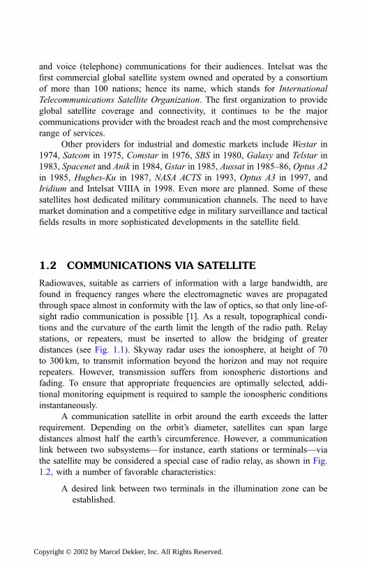
tions and the curvature of the earth limit the length of the radio path. Relay
stations, or repeaters, must be inserted to allow the bridging of greater
distances (see Fig. 1.1). Skyway radar uses the ionosphere, at height of 70
to 300 km, to transmit information beyond the horizon and may not require
repeaters. However, transmission suffers from ionospheric distortions and
fading. To ensure that appropriate frequencies are optimally selected, addi-
tional monitoring equipment is required to sample the ionospheric conditions
instantaneously.
A communication satellite in orbit around the earth exceeds the latter
requirement. Depending on the orbit’s diameter, satellites can span large
distances almost half the earth’s circumference. However, a communication
link between two subsystems—for instance, earth stations or terminals—via
the satellite may be considered a special case of radio relay, as shown in Fig.
1.2, with a number of favorable characteristics:
A desired link between two terminals in the illumination zone can be
established.
Copyright © 2002 by Marcel Dekker, Inc. All Rights Reserved.
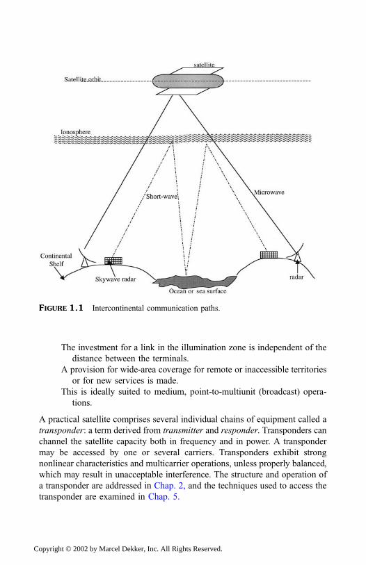
The investment for a link in the illumination zone is independent of the
distance between the terminals.
A provision for wide-area coverage for remote or inaccessible territories
or for new services is made.
This is ideally suited to medium, point-to-multiunit (broadcast) opera-
tions.
A practical satellite comprises several individual chains of equipment called a
transponder: a term derived from transmitter and responder. Transponders can
channel the satellite capacity both in frequency and in power. A transponder
may be accessed by one or several carriers. Transponders exhibit strong
nonlinear characteristics and multicarrier operations, unless properly balanced,
which may result in unacceptable interference. The structure and operation of
a transponder are addressed in Chap. 2, and the techniques used to access the
transponder are examined in Chap. 5.
FIGURE 1.1 Intercontinental communication paths.
Copyright © 2002 by Marcel Dekker, Inc. All Rights Reserved.
1.3 CHARACTERISTIC FEATURES OFCOMMUNICATION SATELLITES
Satellite communication circuits have several characteristic features. These
include
1. Circuits that traverse essentially the same radiofrequency (RF)
pathlength regardless of the terrestrial distance between the term-
inals.
2. Circuits positioned in geosynchronous orbits may suffer a transmis-
sion delay, td , of about 119ms between an earth terminal and the
satellite, resulting in a user-to-user delay of 238ms and an echo
delay of 476ms.
For completeness, transmission delay is calculated using
td ¼h0
cð1:1Þ
where h0 is the altitude above the subsatellite point on the earth
terminal and c is the speed of light (c ¼ 3� 108 m=sec).For example, consider a geostationary satellite whose altitude h0above the subsatellite point on the equator is 35,784 km. This gives
a one-way transmission delay of 119msec, or a roundtrip transmis-
sion delay of 238msec. It should be noted that an earth terminal not
located at the subsatellite point would have greater transmission
delays.
FIGURE 1.2 Communication between two earth stations via a satellite.
Copyright © 2002 by Marcel Dekker, Inc. All Rights Reserved.
3. Satellite circuits in a common coverage area pass through a single
RF repeater for each satellite link (more is said of the coverage area,
repeater, and satellite links in Chaps. 2 and 4). This ensures that
earth terminals, which are positioned at any suitable location within
the coverage area, are illuminated by the satellite antenna(s). The
terminal equipment could be fixed or mobile on land or mobile on
ship and aircraft.
4. Although the uplink power level is generally high, the signal
strength or power level of the received downlink signal is consider-
ably low because of
High signal attenuation due to free-space loss
Limited available downlink power
Finite satellite downlink antenna gain, which is dictated by
the required coverage area
For these reasons, the earth terminal receivers must be designed to
work at significantly low RF signal levels. This leads to the use of
the largest antennas possible for a given type of earth terminal
(discussed in Chap. 3) and the provision of low-noise amplifiers
(LNA) located at close proximity to the antenna feed.
5. Messages transmitted via the circuits are to be secured, rendering
them inaccessible to unauthorized users of the system. Message
security is a commerce closely monitored by the security system
designers and users alike. For example, Pretty Good Privacy (PGP),
invented by Philip Zimmerman, is an effective encryption tool [2].
The U.S. government sued Zimmerman for releasing PGP to the
public, alleging that making PGP available to enemies of the United
States could endanger national security. Although the lawsuit was
later dropped, the use of PGP in many other countries is still illegal.
1.4 MESSAGE SECURITY
Customers’ (private and government) increasing demand to protect satellite
message transmission against passive eavesdropping or active tampering has
prompted system designers to make encryption an essential part of satellite
communication system design. Message security can be provided through
cryptographic techniques. Cryptology is the theory of cryptography (i.e., the
art of writing in or deciphering secret code) and cryptanalysis (i.e., the art of
Copyright © 2002 by Marcel Dekker, Inc. All Rights Reserved.
interpreting or uncovering the deciphered codes without the sender’s consent
or authorization).
Cryptology is an area of special difficulty for readers and students
because many good techniques and analyses are available but remain the
property of organizations whose main business is secrecy. As such, we discuss
the fundamental technique of cryptography in this section without making any
specific recommendations.
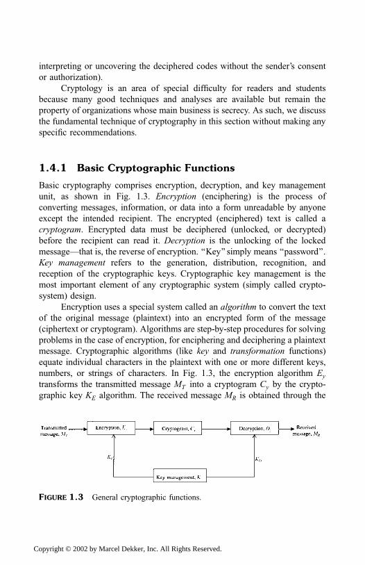
1.4.1 Basic Cryptographic Functions
Basic cryptography comprises encryption, decryption, and key management
unit, as shown in Fig. 1.3. Encryption (enciphering) is the process of
converting messages, information, or data into a form unreadable by anyone
except the intended recipient. The encrypted (enciphered) text is called a
cryptogram. Encrypted data must be deciphered (unlocked, or decrypted)
before the recipient can read it. Decryption is the unlocking of the locked
message—that is, the reverse of encryption. ‘‘Key’’ simply means ‘‘password’’.
Key management refers to the generation, distribution, recognition, and
reception of the cryptographic keys. Cryptographic key management is the
most important element of any cryptographic system (simply called crypto-
system) design.
Encryption uses a special system called an algorithm to convert the text
of the original message (plaintext) into an encrypted form of the message
(ciphertext or cryptogram). Algorithms are step-by-step procedures for solving
problems in the case of encryption, for enciphering and deciphering a plaintext
message. Cryptographic algorithms (like key and transformation functions)
equate individual characters in the plaintext with one or more different keys,
numbers, or strings of characters. In Fig. 1.3, the encryption algorithm Ey
transforms the transmitted message MT into a cryptogram Cy by the crypto-
graphic key KE algorithm. The received message MR is obtained through the
FIGURE 1.3 General cryptographic functions.
Copyright © 2002 by Marcel Dekker, Inc. All Rights Reserved.
decryption algorithm Dy with the corresponding decryption key KD algorithm.
These cryptographic functions are concisely written as follows.
Encryption:
Cy ¼ EyðMT ;KEÞ ð1:2ÞDecryption:
MR ¼ DyðCy;KDÞ¼ DyðEyðMT ;KEÞ;KDÞ
ð1:3Þ
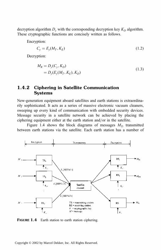
1.4.2 Ciphering in Satellite CommunicationSystems
New-generation equipment aboard satellites and earth stations is extraordina-
rily sophisticated. It acts as a series of massive electronic vacuum cleaners,
sweeping up every kind of communication with embedded security devices.
Message security in a satellite network can be achieved by placing the
ciphering equipment either at the earth station and=or in the satellite.
Figure 1.4 shows the block diagrams of messages MTi transmitted
between earth stations via the satellite. Each earth station has a number of
FIGURE 1.4 Earth station to earth station ciphering.
Copyright © 2002 by Marcel Dekker, Inc. All Rights Reserved.

cryptographic keys Kti (where i ¼ 1; 2; . . . ; n) shared between the commu-
nicating earth stations while the satellite remains transparent: meaning the
satellite has no role in the ciphering process.
A cryptosystem that may work for the scenario depicted by Fig. 1.4 is
described as follows. All the earth stations TS(i) and RS( j) are assumed
capable of generating random numbers RDN(i) and RDN( j), respectively.
Each transmitting earth station TS(i) generates and stores the random numbers
RDN(i). It then encrypts RDN(i), that is, Ey½RDNðiÞ�, and transmits the
encrypted random number Ey½RDNðiÞ� to RS( j). The receiving earth station
RS( j) generates RDN( j) and performs modulo-2 (simply, mod-2) addition
with RDN(i); that is, RDNð jÞ � RDNðiÞ to obtain the session key Krð jÞ,where � denotes mod-2 addition. It should be noted that mod-2 addition is
implemented with exclusive-OR gates and obeys the ordinary rules of addition
except that 1� 1 ¼ 0.
The transmitting earth station retrieves RDN(i) and performs mod-2
addition with RDN( j) (that is, RDNðiÞ � RDNð jÞ) to obtain the session key
KtðiÞ. This process is reversed if RSð jÞ transmits messages and TSðiÞ receives.Figure 1.5 demonstrates the case where the satellite plays an active
ciphering role. In it the keys KEi (where i ¼ 1; 2; . . . ; nÞ the satellite receives
from the transmitting uplink stations TSi are recognized by the onboard
processor, which in turn arranges, ciphers, and distributes to the downlink
FIGURE 1.5 Ciphering with keyed satellite onboard processors.
Copyright © 2002 by Marcel Dekker, Inc. All Rights Reserved.
earth stations, RS( j) (more is said about onboard processing in Chap. 2). Each
receiving earth station has matching cryptographic keys KDj (where
j ¼ l;m; . . . ; zÞ to be able to decipher the received messages MRj.
The cryptosystem that may work for the scenario depicted in Fig. 1.5 is
described as follows. It is assumed that the satellite onboard processor is
capable of working the cryptographic procedures of the satellite network. It is
also assumed that all earth stations TS(i) and RS( j) play passive roles and only
respond to the requests of the satellite onboard processor. The key session of
the onboard processor is encrypted under the station master key. The onboard
processor’s cryptographic procedure provides the key session for recognizing
the key session of each earth station. Thus, when an earth station receives
encrypted messages from the satellite, the earth station’s master key is
retrieved from storage. Using the relevant working key to recognize the
session key activates the decryption procedure. The earth station is ready to
retrieve the original (plaintext) message using the recognized session key.
The European Telecommunication satellite (EUTELSAT) has imple-
mented encryption algorithms, such as the Data Encryption Standard (DES),
as a way of providing security for its satellite link (more is said about DES in
Sec. 1.4.3).
Having discussed the session key functions K, the next item to discuss is
the basic functionality of ciphering techniques and transformation functions.
1.4.3 Ciphering Techniques
Two basic ciphering techniques fundamental to secret system design are
discussed in this section: block ciphering and feedback ciphering.
Block Ciphering
Block ciphering is a process by which messages are encrypted and decrypted
in blocks of information digits. Block ciphering has the same fundamental
structure as block coding for error correction (block coding is further
discussed in Chap. 6). Comparatively, a ciphering system consists of an
encipher and a decipher, while a coding system consists of an encoder and a
decoder. The major difference between the two systems (ciphering and block
coding) is that block ciphering is achieved by ciphering keys while coding
relies on parity checking. A generalized description of a block ciphering
technique is shown in Fig. 1.6. In block ciphering, system security is achieved
by
Copyright © 2002 by Marcel Dekker, Inc. All Rights Reserved.
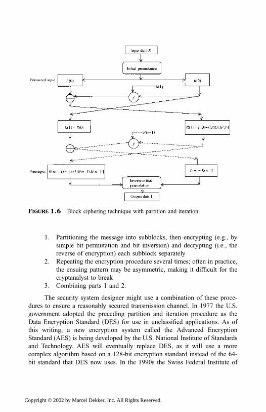
1. Partitioning the message into subblocks, then encrypting (e.g., by
simple bit permutation and bit inversion) and decrypting (i.e., the
reverse of encryption) each subblock separately
2. Repeating the encryption procedure several times; often in practice,
the ensuing pattern may be asymmetric, making it difficult for the
cryptanalyst to break
3. Combining parts 1 and 2.
The security system designer might use a combination of these proce-
dures to ensure a reasonably secured transmission channel. In 1977 the U.S.
government adopted the preceding partition and iteration procedure as the
Data Encryption Standard (DES) for use in unclassified applications. As of
this writing, a new encryption system called the Advanced Encryption
Standard (AES) is being developed by the U.S. National Institute of Standards
and Technology. AES will eventually replace DES, as it will use a more
complex algorithm based on a 128-bit encryption standard instead of the 64-
bit standard that DES now uses. In the 1990s the Swiss Federal Institute of
FIGURE 1.6 Block ciphering technique with partition and iteration.
Copyright © 2002 by Marcel Dekker, Inc. All Rights Reserved.
Technology developed an advanced encryption system based on 128-bit
segments, called the International Data Encryption Algorithm, or IDEA.
This type of encryption is meant for transaction security. Banks in the
United States and several European countries use the IDEA standard for
many of their transactions.
The DES system uses public-key encryption [3]. In a DES system, each
person gets two keys: a public key and a private key. The keys allow a person
to either lock (encrypt) a message or unlock (decipher) an enciphered
message. Each person’s public key is published, and the private key is kept
secret. Messages are encrypted using the intended recipient’s public key and
can only be decrypted using the private key, which is never shared. It is
virtually impossible to determine the private key even if you know the public
key. In addition to encryption, public-key cryptography can be used for
authentication; that is, providing a digital signature that proves a sender
and=or the identity of the recipient. There are other public-key cryptosystems,
such as trapdoor [4], the Rivest–Shamir–Adleman (RSA) system [5], and
McEliece’s system [6].
The basic algorithm for block ciphering is shown in Fig. 1.6 and
described as follows. Suppose there are nþ 1 iterations to be performed.
Denote the input and output data by X ¼ x1, x2, x3; . . . ; xm and Y ¼ y1, y2,
y3; . . . ; ym, y1, y2, y3; . . . ; ym, respectively. Since the input data to be
transformed iteratively is nþ 1 times, the block of data is divided equally
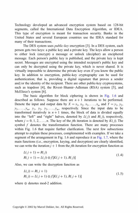
into the ‘‘left’’ and ‘‘right’’ halves, denoted by Lð jÞ and Rð jÞ, respectively,where j ¼ 0; 1; 2; . . . ; n. The key of the jth iteration is denoted by Kð jÞ. Thesymbol f denotes the transformation function. There are many processes
within Fig. 1.6 that require further clarification. The next few subsections
attempt to explain these processes, complemented with examples. If we take a
segment of the arrangement in Fig. 1.6 and reproduce it as Fig. 1.7, where the
main functions (i.e., encryption, keying, and decryption) are clearly identified,
we can write the iteration j þ 1 from the jth iteration for encryption function as
Lð j þ 1Þ ¼ Rð jÞRð j þ 1Þ ¼ Lð jÞ � f ½Kð j þ 1Þ;Rð jÞ� ð1:4Þ
Also, we can write the decryption function as
Lð jÞ ¼ Rð j þ 1ÞRð jÞ ¼ Lð j þ 1Þ � f ½Kð j þ 1Þ;Rð j þ 1Þ� ð1:5Þ
where � denotes mod-2 addition.
Copyright © 2002 by Marcel Dekker, Inc. All Rights Reserved.
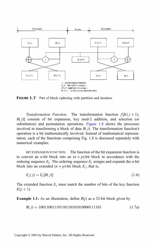
Transformation Function. The transformation function f ½Kð j þ 1Þ,Rð jÞ� consists of bit expansion, key mod-2 addition, and selection (or
substitution) and permutation operations. Figure 1.8 shows the processes
involved in transforming a block of data Rð jÞ. The transformation function’s
operation is a bit mathematically involved. Instead of mathematical represen-
tation, each of the functions comprising Fig. 1.8 is discussed separately with
numerical examples.
BIT EXPANSION FUNCTION. The function of the bit expansion function is
to convert an n-bit block into an ðnþ pÞ-bit block in accordance with the
ordering sequence Ef . The ordering sequence Ef assigns and expands the n-bit
block into an extended ðnþ pÞ-bit block Ex; that is,
Exð jÞ ¼ Ef ½Rð jÞ� ð1:6Þ
The extended function Ex must match the number of bits of the key function
Kðj þ 1Þ.
Example 1.1: As an illustration, define RðjÞ as a 32-bit block given by
Rð jÞ ¼ 10011001110110110101010000111101 ð1:7aÞ
FIGURE 1.7 Part of block ciphering with partition and iteration.
Copyright © 2002 by Marcel Dekker, Inc. All Rights Reserved.
The bit expansion function can be solved by partitioning Rð jÞ into
eight segments (columns) with four bits in each segment. Ensure that
each of the end bits of the segment is assigned to two positions, with the
exception of the first and last bits, thus ensuring the ordering sequence of a
48-bit block:
Ef ¼
32 1 2 3 4 5
4 5 6 7 8 9
8 9 10 11 12 13
12 13 14 15 16 17
16 17 18 19 20 21
20 21 22 23 24 25
24 25 26 27 28 29
28 29 30 31 32 1
ð1:7bÞ
FIGURE 1.8 Sequence of the transformation function.
Copyright © 2002 by Marcel Dekker, Inc. All Rights Reserved.
Based on the ordering sequence of (1.7b), the bit expansion function of (1.6)
becomes
Exð jÞ ¼ Ef ½Rð jÞ� ¼
1 1 0 0 1 11 1 0 0 1 11 1 0 1 1 01 0 1 1 0 10 1 0 1 0 10 1 0 0 0 00 0 1 1 1 11 1 0 1 1 0
0BBBBBBBB@
1CCCCCCCCA
ð1:8Þ
which equates to 48 bits, matching the number of bits of the key function
Kð j þ 1Þ.SELECTION FUNCTION. For simplicity, consider an 8-bit selection
function Sfj, where j ¼ 1; 2; . . . ; 8. Each function has l rows and (mþ 1)
columns. The elements of selection function Sfj have a specific arrangement of
any set of integers from 0 to m. From Example 1.1, each function Sfj takes a 6-
bit block as its input, Sin, denoted by
Sin ¼ x1; x2; x3; x4; x5; x6 ð1:9ÞSuppose rj and cj correspond to a particular row and column of selection
function Sfj. Row rj is determined by the first and last digits of Sin; that is, ðx1,x6). Since x1 and x6 are binary digits, it follows that there can be only four
possible outcomes to indicate the four rows (l ¼ 4) of Sfj while the other four
binary digits (x2, x3, x4, x5) will provide numbers between 0 and m, thereby
determining cj. The intersection of rj and cj in Sfj produces a specific integer
between 0 and m, which, when converted to its binary digits, gives the output
Sop ¼ y1; y2; y3; y4 ð1:10ÞIn practice, the elements of the selection functions Sfj are tabulated like a
lookup table. In the case of DES, l ¼ 4 and m ¼ 15; these elements are shown
in Table 1.1. As seen in Table 1.1, each selection function Sfj has 4-bit output,
giving a total of 32 bits for all selection functions. Example 1.2 demonstrates
how the selection function’s algorithm is implemented.
Example 1.2: Take a row from (1.8), say the first row, as input data; that is,
Sin ¼ 110011. It follows that rj ¼ ðx1; x6Þ ¼ 11 and cj ¼ 1001 ¼ 9. Our task
now is to provide the output Sop due to Sin using the previous transformation
process on the basis of the selection functions given by Table 1.1. If we let
j ¼ 8, the element of S8 in the 4th row and 9th column is 15, which equates to
the digital output Sop ¼ y1, y2, y3, y4 ¼ 1111.
Copyright © 2002 by Marcel Dekker, Inc. All Rights Reserved.
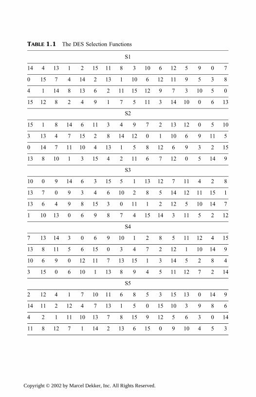
TABLE 1.1 The DES Selection Functions
S1
14 4 13 1 2 15 11 8 3 10 6 12 5 9 0 7
0 15 7 4 14 2 13 1 10 6 12 11 9 5 3 8
4 1 14 8 13 6 2 11 15 12 9 7 3 10 5 0
15 12 8 2 4 9 1 7 5 11 3 14 10 0 6 13
S2
15 1 8 14 6 11 3 4 9 7 2 13 12 0 5 10
3 13 4 7 15 2 8 14 12 0 1 10 6 9 11 5
0 14 7 11 10 4 13 1 5 8 12 6 9 3 2 15
13 8 10 1 3 15 4 2 11 6 7 12 0 5 14 9
S3
10 0 9 14 6 3 15 5 1 13 12 7 11 4 2 8
13 7 0 9 3 4 6 10 2 8 5 14 12 11 15 1
13 6 4 9 8 15 3 0 11 1 2 12 5 10 14 7
1 10 13 0 6 9 8 7 4 15 14 3 11 5 2 12
S4
7 13 14 3 0 6 9 10 1 2 8 5 11 12 4 15
13 8 11 5 6 15 0 3 4 7 2 12 1 10 14 9
10 6 9 0 12 11 7 13 15 1 3 14 5 2 8 4
3 15 0 6 10 1 13 8 9 4 5 11 12 7 2 14
S5
2 12 4 1 7 10 11 6 8 5 3 15 13 0 14 9
14 11 2 12 4 7 13 1 5 0 15 10 3 9 8 6
4 2 1 11 10 13 7 8 15 9 12 5 6 3 0 14
11 8 12 7 1 14 2 13 6 15 0 9 10 4 5 3
Copyright © 2002 by Marcel Dekker, Inc. All Rights Reserved.

PERMUTATION FUNCTION. The purpose of the permutation function Pf
of Fig. 1.8 is to take all the selection function’s 32 bits and permute the digits
to produce a 32-bit block output. The permutation function Pf simply
performs
Z ¼ Pf ðY Þ ð1:11Þwhere the permutation is like the ordering sequence of the ‘‘expansion
function’’:
Pf ¼
16 7 20 2129 12 28 171 15 23 265 18 31 102 8 24 1432 27 3 919 13 30 622 11 4 25
ð1:12aÞ
TABLE 1.1 (continued )
S6
12 1 10 15 9 2 6 8 0 13 3 4 14 7 5 11
10 15 4 2 7 12 9 5 6 1 13 14 0 11 3 8
9 14 15 5 2 8 12 3 7 0 4 10 1 13 11 6
4 3 2 12 9 5 15 10 11 14 1 7 6 0 8 13
S7
4 11 2 14 15 0 8 13 3 12 9 7 5 10 6 1
13 0 11 7 4 9 1 10 14 3 5 12 2 15 8 6
1 4 11 13 12 3 7 14 10 15 6 8 0 5 9 2
6 11 13 8 1 4 10 7 9 5 0 15 14 2 3 12
S8
13 2 8 4 6 15 11 1 10 9 3 14 5 0 12 7
1 15 13 8 10 3 7 4 12 5 6 11 0 14 9 2
7 1 4 1 9 12 14 2 0 6 10 13 15 3 5 8
2 1 14 7 4 10 8 13 15 12 9 0 3 5 6 11
Copyright © 2002 by Marcel Dekker, Inc. All Rights Reserved.
and the 32-bit block input is
Y ¼ y1; y2; y3; . . . ; y32 ð1:12bÞHence, on the basis of (1.12), the permutation function can be written as
Z ¼ Pf ðY Þ ¼ y16; y7; y20; y21; y29; . . . ; y4; y25 ð1:13Þwhich suggests that the 32-bit block input (1.12b) is rearranged (permuted)
according to the ordered permutation function given by (1.12a).
Example 1.3: Suppose
Y ¼ 10011001110110110101010000111101
If we rearrange Y according to (1.12a), the output of the permutation function
is
Z ¼ 10101110110011010100110101101010
In summary, the subsection ‘‘Bit Expansion Function’’ has demonstrated the
process by which an input block data Rð jÞ is transformed to produce an output
function, zð jÞ.Feedback Ciphering
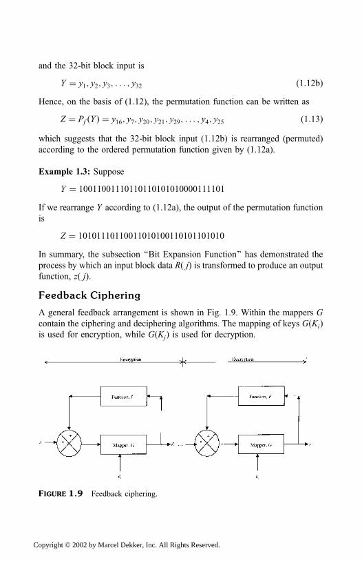
A general feedback arrangement is shown in Fig. 1.9. Within the mappers G
contain the ciphering and deciphering algorithms. The mapping of keys GðKiÞis used for encryption, while GðKjÞ is used for decryption.
FIGURE 1.9 Feedback ciphering.
Copyright © 2002 by Marcel Dekker, Inc. All Rights Reserved.
For an uncoded message x and the feedback function F, the encrypted
message z can be written as
z ¼ ½x� zF�GðKiÞ ð1:14ÞRearranging (1.14) in terms of z, we have
z½1� FGðKiÞ� ¼ xGðKiÞ ð1:15aÞor
z ¼ GðKiÞ1� FGðKiÞ
x ð1:15bÞ
For the decryption circuit, the expression for the decrypted message x can be
written as
x ¼ ½z� xF�GðKjÞ ð1:16aÞAlternatively, in terms of encrypted message z,
z ¼ 1� FGðKjÞGðKjÞ
x ð1:16bÞ
For the same transmission sequence, (1.15b) and (1.16b) must be equal; that
is,
1� FGðKjÞGðKjÞ
¼ GðKiÞ1� FGðKiÞ
ð1:17Þ
which turns to
GðKiÞ ¼ 1� FGðKjÞGðKjÞ ¼ 1� FGðKiÞ
ð1:18Þ
It can be seen in (1.18) that the key functions relate to the feedback functions.
If for argument’s sake we let the feedback F equate unity, then the key
functions become an additive inverse of each other. This shows that the
feedback function and the mapping function are linear functions in this type of
ciphering. In general, a feedback mechanism enhances the strength of a
cryptosystem [7].
1.5 SUMMARY
This chapter has briefly introduced the genesis and characteristic features of
communication satellites. A communication satellite is basically an electronic
Copyright © 2002 by Marcel Dekker, Inc. All Rights Reserved.
communication package placed in orbit whose prime objective is to initiate or
assist the communication transmission of information or a message from one
point to another through space. The information transferred most often
corresponds to voice (telephone), video (television), and digital data.
As electronic forms of communication, commerce, and information
storage and processing have developed, the opportunities to intercept and read
confidential information have grown, and the need for sophisticated encryption
has increased. This chapter has also explained basic cryptographic techniques.
Many newer cryptography techniques being introduced to the market are
highly complex and nearly unbreakable, but their designers and users alike
carefully guard their secrets.
The use of satellites for communication has been steadily increasing,
and more frontiers will be broken as advances in technology make system
production costs economical.
REFERENCES
1. Dressler, W. (1987). Satellite communications, in Siemens Telecom report, vol. 10.
2. Meyer, C. and Matyas, S. (1982). Cryptography: A New Dimension in Computer
Data Security. John Wiley.
3. National Bureau of Standards (1977). Data Encryption Standard. Federal Infor-
mation Processing Standard, Publication 46, U.S. Dep. of Commerce.
4. Diffie, W. and Hellman, M. (1976). New directions in cryptography, IEEE
Transactions on Communications Tech., 29:11, 644–654.
5. Rivest, R., Shamir, A., and Adleman, L. (1978). A method for obtaining digital
signatures and public-key cryptosystems, Communications for the ACM 21:2,
120–126.
6. McEliece, R. (1977). The theory of information and coding, in Encyclopedia of
Mathematics and Its Applications. Addison-Wesley.
7. Wu, W.W. (1985). Elements of Digital Satellite Communication. Computer
Science Press.
PROBLEMS
1. The role of telecommunications networks has changed over the last decade.
(a) Discuss the role of telecommunications networks in modern society.
(b) How has this changed your perception in terms of security, social
cohesion, and commerce?
Copyright © 2002 by Marcel Dekker, Inc. All Rights Reserved.

2. Your task is to develop a communication network covering some inhos-
pitable terrain. What sort of telecommunication infrastructure would you
suggest? Discuss the social, legal, and political implications of the
recommended telecommunication network(s).
3. A packet-switched network is to be designed with onboard processing
capability. Design a suitable cryptosystem for securing the information flow
and message contents.
Copyright © 2002 by Marcel Dekker, Inc. All Rights Reserved.
2
Satellites
2.1 OVERVIEW
A satellite is a radiofrequency repeater. New-generation satellites are regen-
erative; that is, they have onboard processing capability making them more of
an intelligent unit than a mere repeater (more is said of onboard processing in
Sec. 2.9). This capability enables the satellite to condition, amplify, or
reformat received uplink data and route the data to specified locations, or
actually regenerate data onboard the spacecraft as opposed to simply acting as
a relay station between two or more ground stations.
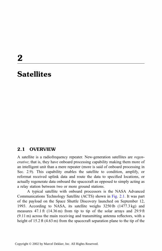
A typical satellite with onboard processors is the NASA Advanced
Communications Technology Satellite (ACTS) shown in Fig. 2.1. It was part
of the payload on the Space Shuttle Discovery launched on September 12,
1993. According to NASA, its satellite weighs 3250 lb (1477.3 kg) and
measures 47.1 ft (14.36m) from tip to tip of the solar arrays and 29.9 ft
(9.11m) across the main receiving and transmitting antenna reflectors, with a
height of 15.2 ft (4.63m) from the spacecraft separation plane to the tip of the
Copyright © 2002 by Marcel Dekker, Inc. All Rights Reserved.
highest antenna. The solar arrays provide approximately 1.4 kilowatts. The
main communication antennas are a 7.2-ft (2.19-m) receiving antenna and a
10.8-ft (3.29-m) transmitting antenna. We describe more about satellite
components’ design later in this chapter, particularly
Overall system design procedure, availability, and reliability in Sec. 2.6
Antennas in Sec. 2.7
Power systems in Sec. 2.8
Onboard processing and switching systems in Sec. 2.9
Antennas control and tracking in Chap. 3, Sec. 3.4.2
Other characteristics of satellites are discussed in the next five sections.
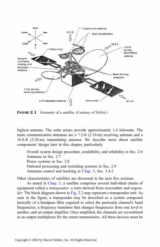
As stated in Chap. 1, a satellite comprises several individual chains of
equipment called a transponder: a term derived from transmitter and respon-
der. The block diagram shown in Fig. 2.2 may represent a transponder unit. As
seen in the figure, a transponder may be described as a system composed
basically of a bandpass filter required to select the particular channel’s band
frequencies, a frequency translator that changes frequencies from one level to
another, and an output amplifier. Once amplified, the channels are recombined
in an output multiplexer for the return transmission. All these devices must be
FIGURE 2.1 Geometry of a satellite. (Courtesy of NASA.)
Copyright © 2002 by Marcel Dekker, Inc. All Rights Reserved.
stable over their operating temperature range to maintain the desired rejection
characteristics. The functionality of these devices (each component block in
Fig. 2.2), is addressed later in this chapter. A transponder may channel the
satellite capacity both in frequency and in power and may be accessed by one
or several carriers.
In most system applications, one satellite serves many earth stations.
With the assistance of earth stations, fixed or transportable, satellites are
opening a new era for global satellite multiaccess channels’ data transmission
and broadcast of major news events, live, from anywhere in the world.
Commercial and operational needs dictate the design and complexity of
satellites. The most common expected satellite attributes include the follow-
ing:
1. Improved coverage areas and quality services, and frequency
reuseability
2. Compatibility of satellite system with other systems and expand-
ability of current system that enhances future operations
3. High-gain, multiple hopping beam antenna systems that permit
smaller-aperture earth stations
4. Increased capacity requirements that allow several G=sec commu-
nication between users
5. Competitive pricing
FIGURE 2.2 Basic transponder arrangement.
Copyright © 2002 by Marcel Dekker, Inc. All Rights Reserved.
Future trends in satellite antennas (concerning design and complexity) are
likely to be dictated from the status of the satellite technology, traffic growth,
emerging technology, and commercial activities.
The next two sections examine the type of satellites and the major
characteristics that determine the satellite path relative to the earth. These
characteristics are as follows:
1. Orbital eccentricity of the selected orbit
2. Period of the orbit
3. Elevation angle; the inclination of the orbital plane relative to the
reference axis
2.1.1 Types of Satellites
There are, in general, four types of satellite:
Geostationary satellite (GEO)
High elliptical orbiting satellite (HEO)
Middle-earth orbiting satellite (MEO)
Low-earth-orbiting satellite (LEO)
An HEO satellite is a specialized orbit in which a satellite continuously swings
very close to the earth, loops out into space, and then repeats its swing by the
earth. It is an elliptical orbit approximately 18,000 to 35,000 km above the
earth’s surface, not necessarily above the equator. HEOs are designed to give
better coverage to countries with higher northern or southern latitudes.
Systems can be designed so that the apogee is arranged to provide continuous
coverage in a particular area. By definition, an apogee is the highest altitude-
point of the orbit, that is, the point in the orbit where the satellite is farthest
from the earth. To clarify some of the terminology, we provide, Fig. 2.3, which
shows the geometric properties of an elliptical orbit. By geometry,
Sm ¼ affiffiffiffiffiffiffiffiffiffiffiffiffi1� e2p
ð2:1ÞSp ¼
Sm
a¼ að1� e2Þ ð2:2Þ
where the eccentricity, or the amount by which the ellipse departs from a
circle, is
e ¼ Sf
að2:3Þ
Copyright © 2002 by Marcel Dekker, Inc. All Rights Reserved.
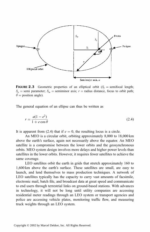
The general equation of an ellipse can thus be written as
r ¼ að1� e2Þ1þ e cos y
ð2:4Þ
It is apparent from (2.4) that if e ¼ 0, the resulting locus is a circle.
An MEO is a circular orbit, orbiting approximately 8,000 to 18,000 km
above the earth’s surface, again not necessarily above the equator. An MEO
satellite is a compromise between the lower orbits and the geosynchronous
orbits. MEO system design involves more delays and higher power levels than
satellites in the lower orbits. However, it requires fewer satellites to achieve the
same coverage.
LEO satellites orbit the earth in grids that stretch approximately 160 to
1,600 km above the earth’s surface. These satellites are small, are easy to
launch, and lend themselves to mass production techniques. A network of
LEO satellites typically has the capacity to carry vast amounts of facsimile,
electronic mail, batch file, and broadcast data at great speed and communicate
to end users through terrestrial links on ground-based stations. With advances
in technology, it will not be long until utility companies are accessing
residential meter readings through an LEO system or transport agencies and
police are accessing vehicle plates, monitoring traffic flow, and measuring
truck weights through an LEO system.
FIGURE 2.3 Geometric properties of an elliptical orbit (Sf ¼ semifocal length;
Sp ¼ semi parameter; Sm ¼ semiminor axis; r ¼ radius distance, focus to orbit path;
y ¼ position angle).
Copyright © 2002 by Marcel Dekker, Inc. All Rights Reserved.
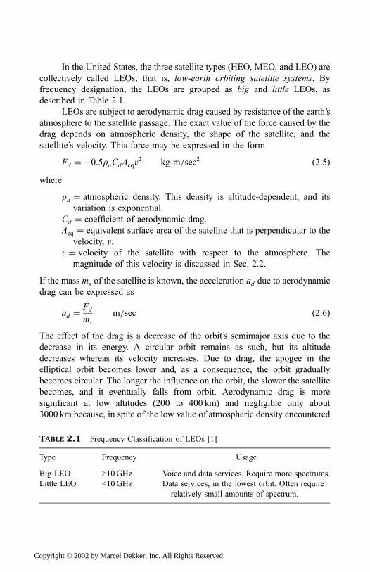
In the United States, the three satellite types (HEO, MEO, and LEO) are
collectively called LEOs; that is, low-earth orbiting satellite systems. By
frequency designation, the LEOs are grouped as big and little LEOs, as
described in Table 2.1.
LEOs are subject to aerodynamic drag caused by resistance of the earth’s
atmosphere to the satellite passage. The exact value of the force caused by the
drag depends on atmospheric density, the shape of the satellite, and the
satellite’s velocity. This force may be expressed in the form
Fd ¼ �0:5raCdAeqv2 kg-m=sec2 ð2:5Þ
where
ra ¼ atmospheric density. This density is altitude-dependent, and its
variation is exponential.
Cd ¼ coefficient of aerodynamic drag.
Aeq ¼ equivalent surface area of the satellite that is perpendicular to the
velocity, v.
v ¼ velocity of the satellite with respect to the atmosphere. The
magnitude of this velocity is discussed in Sec. 2.2.
If the mass ms of the satellite is known, the acceleration ad due to aerodynamic
drag can be expressed as
ad ¼Fd
ms
m=sec ð2:6Þ
The effect of the drag is a decrease of the orbit’s semimajor axis due to the
decrease in its energy. A circular orbit remains as such, but its altitude
decreases whereas its velocity increases. Due to drag, the apogee in the
elliptical orbit becomes lower and, as a consequence, the orbit gradually
becomes circular. The longer the influence on the orbit, the slower the satellite
becomes, and it eventually falls from orbit. Aerodynamic drag is more
significant at low altitudes (200 to 400 km) and negligible only about
3000 km because, in spite of the low value of atmospheric density encountered
TABLE 2.1 Frequency Classification of LEOs [1]
Type Frequency Usage
Big LEO >10GHz Voice and data services. Require more spectrums.
Little LEO <10GHz Data services, in the lowest orbit. Often require
relatively small amounts of spectrum.
Copyright © 2002 by Marcel Dekker, Inc. All Rights Reserved.

at the altitudes of satellites, their high orbital velocity implies that perturba-
tions due to drag are very significant.
A geostationary orbit is a nonretrograde circular orbit in the equatorial
plane with zero eccentricity and zero inclination. The satellite remains fixed
(stationary) in an apparent position relative to the earth; about 35,784 km away
from the earth if its elevation angle is orthogonal (90�) to the equator. Its
period of revolution is synchronized with that of the earth in inertial space.
The geometric considerations for a geostationary satellite communication
system are discussed later in the text.
Commercial GEOs provide fixed satellite service (FSS) in the C and Ku
bands of the radio spectrum. Some GEOs use the Ku band to provide certain
mobile services. The International Telecommunication Union (ITU) (see Chap.
7) has allocated satellite bands in various parts of the radio spectrum from
VHF to 275GHz. Table 2.2 shows satellite communications frequency bands
and the services they perform, while Table 2.3 shows typical links frequency
bands.
Frequency bands in the UHF are suitable for communicating with small
or mobile terminals, for television broadcasting, and for military fleet
communication. The band of frequencies suitable for an earth–space–earth
radio link is between 450MHz and 20GHz. Frequencies between 20 and
50GHz can be used but would be subject to precipitation attenuation.
However, if an availability greater than 99.5% is required, a special provision
such as diversity reception and adaptive power control would need to be
TABLE 2.2 Communication Satellite Frequency Bands Allocation
Band Frequency range (GHz) Services
VHF 0.03–0.3 Messaging
UHF 0.3–1.0 Military, navigation mobile
L 1–2 Mobile, audio broadcast radiolo-
cation
S 2–4 Mobile navigation
C 4–8 Fixed
X 8–12 Military
Ku 12–18 Fixed video broadcast
K 18–27 Fixed
Ka 27–40 Fixed, audio broadcast, intersatel-
lite
mm waves >40 Intersatellite
Copyright © 2002 by Marcel Dekker, Inc. All Rights Reserved.
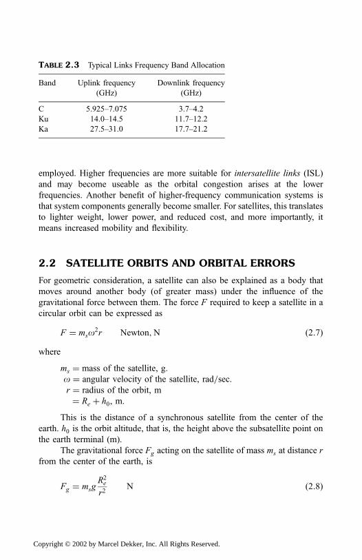
employed. Higher frequencies are more suitable for intersatellite links (ISL)
and may become useable as the orbital congestion arises at the lower
frequencies. Another benefit of higher-frequency communication systems is
that system components generally become smaller. For satellites, this translates
to lighter weight, lower power, and reduced cost, and more importantly, it
means increased mobility and flexibility.
2.2 SATELLITE ORBITS AND ORBITAL ERRORS
For geometric consideration, a satellite can also be explained as a body that
moves around another body (of greater mass) under the influence of the
gravitational force between them. The force F required to keep a satellite in a
circular orbit can be expressed as
F ¼ mso2r Newton;N ð2:7Þ
where
ms ¼ mass of the satellite, g.
o ¼ angular velocity of the satellite, rad=sec.r ¼ radius of the orbit, m
¼ Re þ h0, m.
This is the distance of a synchronous satellite from the center of the
earth. h0 is the orbit altitude, that is, the height above the subsatellite point on
the earth terminal (m).
The gravitational force Fg acting on the satellite of mass ms at distance r
from the center of the earth, is
Fg ¼ msgR2e
r2N ð2:8Þ
TABLE 2.3 Typical Links Frequency Band Allocation
Band Uplink frequency Downlink frequency
(GHz) (GHz)
C 5.925–7.075 3.7–4.2
Ku 14.0–14.5 11.7–12.2
Ka 27.5–31.0 17.7–21.2
Copyright © 2002 by Marcel Dekker, Inc. All Rights Reserved.
where
g ¼ acceleration due to gravity at the surface of the earth
¼ 9:8087m=sec2.Re ¼ radius of the earth. The value varies with location. For example,
Re at the equator ¼ 6378.39 km (6378 km).
Re at the pole ¼ 6356.91 km (6357 km).
Consequently, for a satellite in a stable circular orbit around the earth,
F ¼ Fg ð2:9ÞIn view of (2.7) and (2.8) in (2.9),
r3 ¼ gR2e
o2ð2:10Þ
The period of the orbit, ts, that is, the time taken for one complete revolution
(360� or 2p radians), can be expressed as
ts ¼2po¼ 2p
Re
ffiffiffiffir3
g
ssec ð2:11Þ
If we assume a spherical homogeneous earth, a satellite will have an orbital
velocity represented by
v ¼ Re
ffiffiffig
r
rm=sec ð2:12Þ
For elliptical orbits, Eqs. (2.11) and (2.12) are also valid by equating the
ellipse semimajor axis, a with the orbit radius r (i.e., r ¼ a). In terms of the
orbit parameters, r is replaced with the average of apogee to focus and perigee
to focus. By definition, a perigee is the lowest altitude point of the orbit,
whereas an apogee is the highest altitude point of the orbit. In a circular orbit,
with variable altitude and upon substitution of empirical values in (2.11) and
(2.12), Fig. 2.4, which relates period and velocity for circular orbits, assuming
a spherical homogeneous earth, is plotted.
For a circular orbit at an altitude of 35,784 km, Fig. 2.4 shows that a
geosatellite orbit takes a period of rotation of the earth relative to the fixed star
(called sidereal day) in 86163.9001 sec, or 23 h, 56min, and 4 sec. In some
books and papers, an approximate value of 36,000 km is frequently cited for
the altitude of the satellite in geosynchronous orbit. The geosynchronous orbit
in the equatorial plane is called the geostationary orbit. Although a satellite in
Copyright © 2002 by Marcel Dekker, Inc. All Rights Reserved.
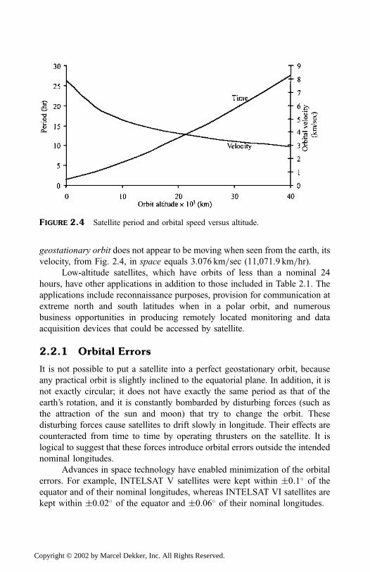
geostationary orbit does not appear to be moving when seen from the earth, its
velocity, from Fig. 2.4, in space equals 3.076 km=sec (11,071.9 km=hr).Low-altitude satellites, which have orbits of less than a nominal 24
hours, have other applications in addition to those included in Table 2.1. The
applications include reconnaissance purposes, provision for communication at
extreme north and south latitudes when in a polar orbit, and numerous
business opportunities in producing remotely located monitoring and data
acquisition devices that could be accessed by satellite.
2.2.1 Orbital Errors
It is not possible to put a satellite into a perfect geostationary orbit, because
any practical orbit is slightly inclined to the equatorial plane. In addition, it is
not exactly circular; it does not have exactly the same period as that of the
earth’s rotation, and it is constantly bombarded by disturbing forces (such as
the attraction of the sun and moon) that try to change the orbit. These
disturbing forces cause satellites to drift slowly in longitude. Their effects are
counteracted from time to time by operating thrusters on the satellite. It is
logical to suggest that these forces introduce orbital errors outside the intended
nominal longitudes.
Advances in space technology have enabled minimization of the orbital
errors. For example, INTELSAT V satellites were kept within �0:1� of theequator and of their nominal longitudes, whereas INTELSAT VI satellites are
kept within �0:02� of the equator and �0:06� of their nominal longitudes.
FIGURE 2.4 Satellite period and orbital speed versus altitude.
Copyright © 2002 by Marcel Dekker, Inc. All Rights Reserved.
2.3 COVERAGE AREA AND SATELLITENETWORKS
2.3.1 Geometric Coverage Area
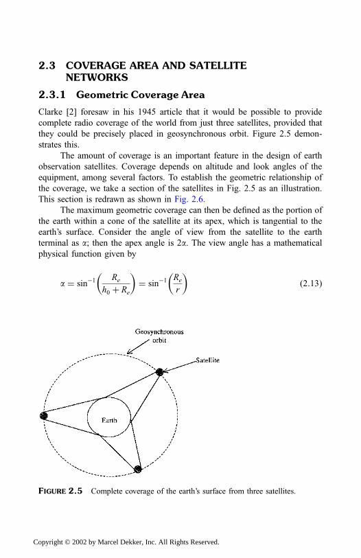
Clarke [2] foresaw in his 1945 article that it would be possible to provide
complete radio coverage of the world from just three satellites, provided that
they could be precisely placed in geosynchronous orbit. Figure 2.5 demon-
strates this.
The amount of coverage is an important feature in the design of earth
observation satellites. Coverage depends on altitude and look angles of the
equipment, among several factors. To establish the geometric relationship of
the coverage, we take a section of the satellites in Fig. 2.5 as an illustration.
This section is redrawn as shown in Fig. 2.6.
The maximum geometric coverage can then be defined as the portion of
the earth within a cone of the satellite at its apex, which is tangential to the
earth’s surface. Consider the angle of view from the satellite to the earth
terminal as a; then the apex angle is 2a. The view angle has a mathematical
physical function given by
a ¼ sin�1Re
h0 þ Re
� �¼ sin�1
Re
r
� �ð2:13Þ
FIGURE 2.5 Complete coverage of the earth’s surface from three satellites.
Copyright © 2002 by Marcel Dekker, Inc. All Rights Reserved.
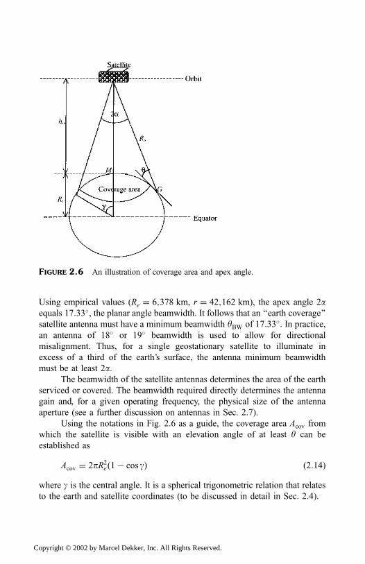
Using empirical values (Re ¼ 6;378 km, r ¼ 42;162 km), the apex angle 2aequals 17:33�, the planar angle beamwidth. It follows that an ‘‘earth coverage’’
satellite antenna must have a minimum beamwidth yBW of 17:33�. In practice,
an antenna of 18� or 19� beamwidth is used to allow for directional
misalignment. Thus, for a single geostationary satellite to illuminate in
excess of a third of the earth’s surface, the antenna minimum beamwidth
must be at least 2a.The beamwidth of the satellite antennas determines the area of the earth
serviced or covered. The beamwidth required directly determines the antenna
gain and, for a given operating frequency, the physical size of the antenna
aperture (see a further discussion on antennas in Sec. 2.7).
Using the notations in Fig. 2.6 as a guide, the coverage area Acov from
which the satellite is visible with an elevation angle of at least y can be
established as
Acov ¼ 2pR2eð1� cos gÞ ð2:14Þ
where g is the central angle. It is a spherical trigonometric relation that relates
to the earth and satellite coordinates (to be discussed in detail in Sec. 2.4).
FIGURE 2.6 An illustration of coverage area and apex angle.
Copyright © 2002 by Marcel Dekker, Inc. All Rights Reserved.
The apex angle required at the satellite to produce a given coverage Acov
must satisfy
2pf1� cos ag ¼ Acov
h20ð2:15Þ
However, for small angles, that is, a 1, we can approximate the global
beamwidth to
2a dcov
h0ð2:16Þ
where dcov is the coverage area diameter.
In order to provide communications among areas serviced by the three
satellites, a terrestrial repeater must be provided at a location where both
satellites are visible. Alternatively, a link can be established between the
satellites (see Section 2.3.2) and using a multibeam satellite configuration (see
Sec. 2.3.3). Also, by using nonsynchronous orbits, the tradeoff between
synchronous and non-synchronous orbits is a complicated system design
problem.
2.3.2 Satellite Constellation
A constellation is a group of similar satellites working together in partnership
to provide a network of useful service. The constellation (or configuration) of
satellites in the LEO system is designed to function as a network primarily to
get more or better coverage. Each satellite in an orbital plane maintains its
position in relation to the other satellites in the plane. Each satellite in an LEO
constellation, for example, acts as a switching node and is connected to nearby
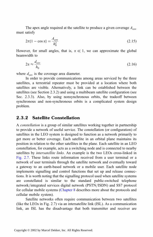
satellites by intersatellite links. An example is the two LEOs cross-linked in
Fig. 2.7. These links route information received from a user terminal or a
network of user terminals through the satellite network and eventually toward
a gateway to an earth-based network or a mobile user. Each satellite node
implements signalling and control functions that set up and release connec-
tions. It is worth noting that the signalling protocol used when satellite systems
are constellated is similar to the standard public-switched telephone
network=integrated services digital network (PSTN=ISDN) and SS7 protocol
for cellular mobile systems (Chapter 8 describes more about the protocols and
cellular mobile system).
Satellite networks often require communication between two satellites
(like the LEOs in Fig. 2.7) via an intersatellite link (ISL). As a communication
link, an ISL has the disadvantage that both transmitter and receiver are
Copyright © 2002 by Marcel Dekker, Inc. All Rights Reserved.
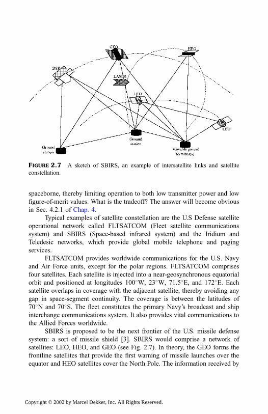
spaceborne, thereby limiting operation to both low transmitter power and low
figure-of-merit values. What is the tradeoff? The answer will become obvious
in Sec. 4.2.1 of Chap. 4.
Typical examples of satellite constellation are the U.S Defense satellite
operational network called FLTSATCOM (Fleet satellite communications
system) and SBIRS (Space-based infrared system) and the Iridium and
Teledesic networks, which provide global mobile telephone and paging
services.
FLTSATCOM provides worldwide communications for the U.S. Navy
and Air Force units, except for the polar regions. FLTSATCOM comprises
four satellites. Each satellite is injected into a near-geosynchronous equatorial
orbit and positioned at longitudes 100�W, 23�W, 71:5�E, and 172�E. Eachsatellite overlaps in coverage with the adjacent satellite, thereby avoiding any
gap in space-segment continuity. The coverage is between the latitudes of
70�N and 70�S. The fleet constitutes the primary Navy’s broadcast and ship
interchange communications system. It also provides vital communications to
the Allied Forces worldwide.
SBIRS is proposed to be the next frontier of the U.S. missile defense
system: a sort of missile shield [3]. SBIRS would comprise a network of
satellites: LEO, HEO, and GEO (see Fig. 2.7). In theory, the GEO forms the
frontline satellites that provide the first warning of missile launches over the
equator and HEO satellites cover the North Pole. The information received by
FIGURE 2.7 A sketch of SBIRS, an example of intersatellite links and satellite
constellation.
Copyright © 2002 by Marcel Dekker, Inc. All Rights Reserved.

the frontline satellites is then passed via dedicated defense support program
(DSP) satellites to earth terminals. The DSP satellites are programmed to look
for the launch flares of a missile taking off or the distinctive double flares that
mark the explosion of a nuclear weapon. The details of the missile trajectories
are then passed to a network of LEOs, which would track the missile warheads
after they separate from their launchers and cruise through space. The space-
based laser system is then activated to track incoming missile(s).
The Iridium network, deployed in 1998, consists of 66 satellites in six
orbital planes [4]. Each satellite has 48 spot beams. The satellite network’s
switching algorithm allows some of the beams to be switched off as it
approaches the poles but maintains a sizeable proportion of the beams at
any given time. Each satellite is connected to four neighboring satellites, and
the intersatellite links operate in the 23.18- to 23.38-GHz band. Communica-
tions between the satellite network and terrestrial network are through ground
station gateways. The uplink and downlink frequency bands to the gateways
are 29.1 to 29.3GHz and 19.2 to 19.6GHz, respectively.
The Teledesic network plans for 288 satellites to be deployed in a
number of polar orbits [5]. Each satellite is interconnected to eight adjacent
satellites to provide tolerance to faults and adaptability to congestion. In this
network the earth is divided into approximately 20,000 square ‘‘supercells’’,
each 160 km long and comprised of 9 square cells. Each satellite’s beam covers
up to 64 supercells; the actual effective supercell coverage depends on the
satellite’s orbital position and its relative distance to other satellites. Each cell
in the supercell is allocated a time slot, and each satellite focuses on the cell in
the supercell at that allotted time. When the beam is directed at a cell, each
terminal in the cell transmits on the uplink, using one or more frequency
channels that have been assigned to it. During this time frame, the satellite
transmits a sequence of packets of terminals in the cells. The terminals in turn
receive all packets and distribute them to respective localities.
2.3.3 Multibeam Satellite Network
Multibeam antennas carried aboard the satellites attempt to conserve available
frequencies. A multibeam antenna transmits a family of pencil-thin beams,
often so small that, by the time they reach the earth’s surface, their footprint
covers an oval only a few tens of kilometers wide. As an illustration, instead of
using a global angular width of 17:33� for one satellite for a global beam
coverage discussed in Sec. 2.3.1, multiple narrow beams, each of an angular
Copyright © 2002 by Marcel Dekker, Inc. All Rights Reserved.
width of 1:73� with reduced coverage and increased gain, are used. This
scheme permits multibeam satellite configuration. This scheme includes the
following advantages:
1. Power is divided among the beams, and the bandwidth remains
constant for each beam. As a result, the total bandwidth increases by
the number of beams.
2. Performance improves as the number of beams increases although
limited by technology and the complexity of the satellite, which
increases with the number of beams.
3. There is extended satellite coverage from the juxtaposition of
several beams, and each beam provides an antenna gain that
increases as the angular beamwidth decreases.
4. Frequency reuse is achieved, which means using the same frequency
band several times so as to increase the overall capacity of the
network without increasing the allocated bandwidth. This can be
achieved by exploiting the isolation resulting from antenna direc-
tivity to reuse the same frequency band in different beams. For
instance, an antenna designed to transmit or receive an electro-
magnetic wave of a given polarization can neither transmit nor
receive in the orthogonal polarization. This property enables two
simultaneous links to be established at the same frequency between
two identical locations. This process is called frequency reuse or
orthogonal polarization. To achieve this feat, either two polarized
antennas must be provided at each end or, preferably, one antenna,
which operates with the two specified polarizations, may be used.
The drawback is that this could lead to mutual interference of the
two links. The magnitude of this interference on the total transmis-
sion link will be examined in Chap. 4.
2.4 GEOMETRIC DISTANCES
By considering the geometry of the geosatellite’s orbit in its orbital plane, we
will be able to calculate
1. The distance between the satellite and earth station, called the slant
range, Rs.
2. The azimuth and elevation angles, collectively called the look
angles. The look angles are the coordinates to which an earth
Copyright © 2002 by Marcel Dekker, Inc. All Rights Reserved.
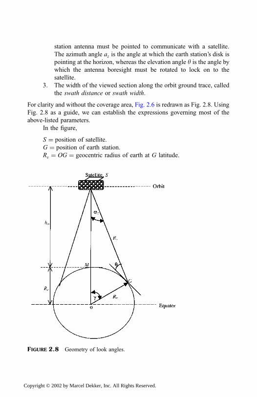
station antenna must be pointed to communicate with a satellite.
The azimuth angle az is the angle at which the earth station’s disk is
pointing at the horizon, whereas the elevation angle y is the angle bywhich the antenna boresight must be rotated to lock on to the
satellite.
3. The width of the viewed section along the orbit ground trace, called
the swath distance or swath width.
For clarity and without the coverage area, Fig. 2.6 is redrawn as Fig. 2.8. Using
Fig. 2.8 as a guide, we can establish the expressions governing most of the
above-listed parameters.
In the figure,
S ¼ position of satellite.
G ¼ position of earth station.
Rv ¼ OG ¼ geocentric radius of earth at G latitude.
FIGURE 2.8 Geometry of look angles.
Copyright © 2002 by Marcel Dekker, Inc. All Rights Reserved.
y ¼ elevation angle of satellite from the earth station.
LET ¼ latitude of the earth station. This value is positive for latitudes in
the Northern Hemisphere (i.e., north of the equator) and negative for
the Southern Hemisphere (i.e., south of the equator).
M ¼ location of subsatellite point. This location’s longitude and latitude
are determined from a satellite ephemeris table. Nominally, latitude is
taken as 0� for geostationary satellite.
LSAT ¼ latitude of the satellite.
D ¼ difference in longitude between the earth station and the satellite.
g ¼ central angle.
r ¼ radius of the orbit ¼ OM þMS ¼ Re þ h0.
Using the spherical trigonometric relations, we determined the central angle
from
g ¼ cos�1ðsinLSAT sin LET þ cos LSAT cos LET cosDÞ ð2:17ÞUsing cosine law, we find the slant range equation to be
Rs ¼ffiffiffiffiffiffiffiffiffiffiffiffiffiffiffiffiffiffiffiffiffiffiffiffiffiffiffiffiffiffiffiffiffiffiffiffiffiffiffiffiR2e þ r2 � 2rRe cos g
pkm ð2:18aÞ
Alternatively,
Rs ¼Rv sin g
cosðgþ yÞ km ð2:18bÞ
The geocentric radius, Rv, may be described by
Rv ¼ Reð0:99832þ 0:001684 cos 2LET � 0:000004 cos 4LET � � �Þ ðkmÞð2:19Þ
The elevation angle y may be written as
y ¼ tan�1cosD cos LET � ðRe=rÞffiffiffiffiffiffiffiffiffiffiffiffiffiffiffiffiffiffiffiffiffiffiffiffiffiffiffiffiffiffiffiffiffiffiffiffiffiffi
1� cos2 D cos2 LETp
!deg ð2:20aÞ
Alternatively,
y ¼ tan�1 cot g� Rv
r sin g
� �deg ð2:20bÞ
The above equations developed for elevation angle y give the geometric value.
The true elevation angle yt, taking into account the average atmospheric
refraction, is given by the approximate equation (Porcelli [6]).
yt ¼ 0:5ðyþffiffiffiffiffiffiffiffiffiffiffiffiffiffiffiffiffiffiffiffiffiffiy2 þ 4:132
pÞ deg ð2:21Þ
Copyright © 2002 by Marcel Dekker, Inc. All Rights Reserved.
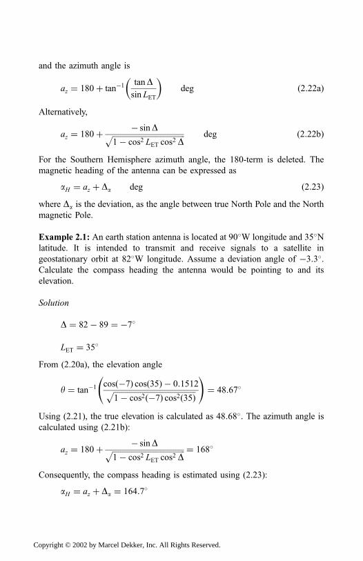
and the azimuth angle is
az ¼ 180þ tan�1tanDsin LET
� �deg ð2:22aÞ
Alternatively,
az ¼ 180þ � sinDffiffiffiffiffiffiffiffiffiffiffiffiffiffiffiffiffiffiffiffiffiffiffiffiffiffiffiffiffiffiffiffiffiffiffiffiffiffi1� cos2 LET cos
2 Dp deg ð2:22bÞ
For the Southern Hemisphere azimuth angle, the 180-term is deleted. The
magnetic heading of the antenna can be expressed as
aH ¼ az þ Da deg ð2:23Þwhere Da is the deviation, as the angle between true North Pole and the North
magnetic Pole.
Example 2.1: An earth station antenna is located at 90�W longitude and 35�Nlatitude. It is intended to transmit and receive signals to a satellite in
geostationary orbit at 82�W longitude. Assume a deviation angle of �3:3�.Calculate the compass heading the antenna would be pointing to and its
elevation.
Solution
D ¼ 82� 89 ¼ �7�
LET ¼ 35�
From (2.20a), the elevation angle
y ¼ tan�1cosð�7Þ cosð35Þ � 0:1512ffiffiffiffiffiffiffiffiffiffiffiffiffiffiffiffiffiffiffiffiffiffiffiffiffiffiffiffiffiffiffiffiffiffiffiffiffiffiffiffiffiffiffi
1� cos2ð�7Þ cos2ð35Þp
!¼ 48:67�
Using (2.21), the true elevation is calculated as 48:68�: The azimuth angle is
calculated using (2.21b):
az ¼ 180þ � sinDffiffiffiffiffiffiffiffiffiffiffiffiffiffiffiffiffiffiffiffiffiffiffiffiffiffiffiffiffiffiffiffiffiffiffiffiffiffi1� cos2 LET cos
2 Dp ¼ 168�
Consequently, the compass heading is estimated using (2.23):
aH ¼ az þ Da ¼ 164:7�
Copyright © 2002 by Marcel Dekker, Inc. All Rights Reserved.
We can conclude that the antenna must be pointed toward a compass heading
of 164:7� and be adjusted to an elevation of 48:68� to transmit or receive
signals from the satellite in the geostationary orbit.
2.5 SWATH WIDTH, COMMUNICATION TIME,AND SATELLITE VISIBILITY
2.5.1 Visibility of Satellites from the Earth
One of the most important pieces of information about a communication
satellite is whether it can be seen from a particular location on the earth. The
use of (2.21) and (2.22b) enables us to interpret the bearings relative to the
local meridian. As an illustration, suppose LET ¼ 40� and D ¼ 50�. Conse-quently, az ¼ 62� and the elevation of the satellite y ¼ 21�. Now, on the one
hand, suppose the satellite is east of the earth station and the station is south of
the equator; the azimuth of the satellite from the station will equal az, that is,
62�E of N. On the other hand, if the station is north of the equator, then the
azimuth of the satellite is ð180� azÞ ¼ 118�E of N. Similarly, if the satellite is
west of the station, then the azimuth of the satellite is ð180þ azÞ ¼ 242�E of
N for the station north of the equator, and finally ð360� azÞ ¼ 298�E of N for
a station south of the equator.
2.5.2 Communication Time
The amount of time tp an earth station is required to communicate with an
orbiting satellite as it passes overhead is given by
tp ¼g
180�� � ts
1� ðts=teÞ� �
ð2:24Þ
where
ts ¼ orbit period.
te ¼ rotation period of the earth ¼ 1 sidereal day.
Note that the sign � depends on whether the satellite is in a retrograde
(opposite-direction) orbit or a prograde (same-direction) orbit. For instance, if
a satellite is in a prograde orbit, te ¼ ts, and as such tp ¼ 1. The expression
(2.24) is valid for a satellite orbiting at altitude h0 and passing over any point
on earth with an elevation angle exceeding y.
Copyright © 2002 by Marcel Dekker, Inc. All Rights Reserved.
2.5.3 Swath Width
The width of the viewed section along the orbit ground trace is called the
swath width. Following the previous assumption of a spherical earth, it can be
demonstrated that the swath width may be written as
ws ¼Re
9090� yBW
2� cos�1
h0Rv
Re
sinyBW2
� �� �ð2:25Þ
where yBW is the antenna beamwidth in degrees. Other symbols are as defined
previously. The above expression can be used to determine the coverage at any
latitude during a particular operation. For practical explanation, when a polar
orbit is used, the percentage coverage at the equator is taken as the ratio of
swath width to the total distance between consecutive passes. To the contrary,
at latitudes beside the equator, the percentage coverage in a given day is the
equatorial coverage divided by the cosine of the latitude.
2.6 SYSTEMS ENGINEERING: DESIGN PROCEDURE
The constraints imposed by the satellite on size, shape, cost, and weight are
important factors in design consideration [7]. A satellite design block diagram
is shown in Fig. 2.9; it shows the flow-down of requirements to system
development. Several factors dictate the satellite system design process, but
some generalizations are possible.
The overriding concern is the cost for developing the system. It is
imperative that system cost-effectiveness analysis be performed, as it supports
the development of the lifecycle of products, processes, and risk management
activities.
2.6.1 Mission Requirements
In general, mission requirements are intended to indicate, as definitively as
practical, the objectives of the mission: what is to be achieved and how to
measure performance. In some cases, the requirements are not clear-cut. It is
the system engineer’s responsibility to (1) ensure that both the customer and
the developer understand the mission objectives and (2) clearly define
practically attainable and practically verifiable results.
Copyright © 2002 by Marcel Dekker, Inc. All Rights Reserved.
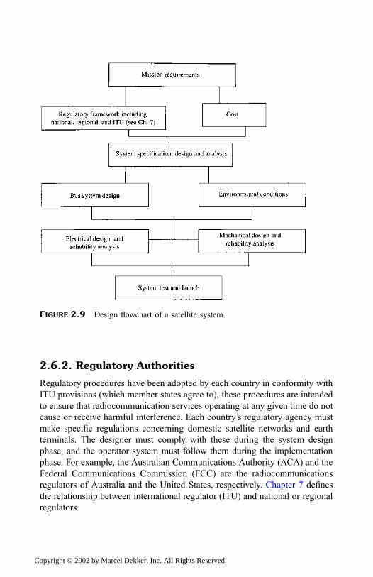
2.6.2. Regulatory Authorities
Regulatory procedures have been adopted by each country in conformity with
ITU provisions (which member states agree to), these procedures are intended
to ensure that radiocommunication services operating at any given time do not
cause or receive harmful interference. Each country’s regulatory agency must
make specific regulations concerning domestic satellite networks and earth
terminals. The designer must comply with these during the system design
phase, and the operator system must follow them during the implementation
phase. For example, the Australian Communications Authority (ACA) and the
Federal Communications Commission (FCC) are the radiocommunications
regulators of Australia and the United States, respectively. Chapter 7 defines
the relationship between international regulator (ITU) and national or regional
regulators.
FIGURE 2.9 Design flowchart of a satellite system.
Copyright © 2002 by Marcel Dekker, Inc. All Rights Reserved.
2.6.3 System Speci¢cations: Analysis and Design
System specifications are essentially sets of dos and don’ts as applied to
system operations and could be labeled as technical requirements in terms of
function, performance, interface, and design requirements for the system,
equipment, and software. The technical requirements may relate to manning,
operating, maintaining, and logistically supporting the system, equipment,
and=or software to the extent that these requirements define or constrain the
design.
It is at this phase that the requirements are dissected and analyzed in
greater detail, covering
1. Description of the methods, procedures, tools for analysis of
mission statement(s), operations, and environment
2. Identification of functional and performance requirements for
design, development, manufacturing, verification, deployment, oper-
ations, support, training, and disposal
3. Determination of system constraints, including description of the
following:
Reliability and maintainability
Survivability
Electromagnetic compatibility, radiofrequency management,
and electrostatic discharge
Human engineering and human systems integration
Safety and health hazards
Test and evaluation
Integrated diagnostics
Other system functionality that has bearing on the determination
of performance and functional requirements for the system
4. Risk management, covering at least the following:
Approach and criteria for risk identification, prioritization,
sensitivity assessment, handling, and risk impact integration
into the decision process
The risks associated with the system development test and
evaluation requirements
Appropriate plans to handle technical risks (for example, those
associated with technology and integration verification,
backup development, etc.)
Copyright © 2002 by Marcel Dekker, Inc. All Rights Reserved.
Risk control and monitoring measures, including technical
performance measurement
Risks associated with cost and schedule performance measure-
ment
5. Environmental factors
The prime environmental problems a satellite encounters are electro-
magnetic charges, radiation, pressure differential, solar radiation or flare, and
other artifacts like meteoroids. The space environment is composed of
electromagnetic and corpuscular radiation. Electromagnetic radiation comes
mainly from the sun and exhibits the properties of waves travelling at the
speed of light. Corpuscular radiation originates both in the sun and in galactic
space and consists of charged and uncharged particles whose velocity is the
product of the mechanics of generation. In essence, environmental conditions
during launch and in space affect mechanical and electrical design as well as
reliability consideration.
Upon completion of these analyses, an operational concept document
(OCD) is produced, whose main purposes are to
1. Specify the system characteristics from an operational perspective.
2. Ensure that users understand the system goals.
3. Provide guidance for development of subsequent system definition
documents such as system specification, interface specification,
product specification, test specification, etc.
4. Describe the user organization and mission from an integrated
system and=or user point of view.
It is important to note that, at this system-level design, the customer’s approval
must be gained for the OCD to become valid because the customer is the
owner of the OCD. The production and subsequent approval of the OCD is the
first step in clarifying the customer’s needs and establishing the customer’s
requirements as well as providing practical guidelines on how to apply these
outlined requirements for system analysis and design.
2.6.4 System Design: Bus, Electrical, and Mechanical
The satellite bus system design must consider the beam pointing accuracy,
velocity, and angular range.
Copyright © 2002 by Marcel Dekker, Inc. All Rights Reserved.
Like all materials that require coupling, all mechanical conditions must
be properly observed. These conditions include accurate dimensioning, overall
weight of the component parts, sinusoidal and random vibration, noise, heat,
dynamic strength, stiffness, acceleration, and launching (or deployment)
shock. These conditions, in some regards, apply to the electrical component’s
design.
To reduce distortions due to heat, the material property must be well
determined and stress-release design properly considered. Modern design
incorporates venting to avoid destruction due to pressure change during
satellite launch.
The electrical design must first consider what type of antenna is
preferred: omnidirectional, single-beam, multibeam, or shaped-beam. Omni-
directional antennas are those that radiate uniformly in all directions. Single-
beam antennas are used as global-beam or spot-beam antennas in satellite
communication antennas. Horn antennas are generally used for global-beam
purposes. Spot-beam antennas usually use larger-aperture diameters to form a
narrow beam; these antennas usually employ reflectors (e.g., the paraboloidal
reflector, horn reflector, Cassegrain reflector, and Gregorian reflector). The
characteristics of these antennas, which are generally applicable to both
satellite and earth stations, are discussed in Sec. 2.7. Shaped-beam antennas
are antennas whose radiated beams are shaped to a prescribed pattern. A
reflector or lens antenna is widely used with multiple-feed elements for
generating a shaped beam for a satellite communication antenna system.
The advantage of beam shaping includes enhancement of the antenna gain and
improvement of beam-to-beam isolation, which is a key parameter for
increasing communication capacity due to frequency reuse.
As demonstrated in Sec. 2.3, the beamwidth of the satellite antenna is
directly related to the size of the coverage area and, for a given operating
frequency, the antenna aperture diameter D. Antenna selection is governed by
the aperture-frequency (D � f ) product, as shown in Table 2.4. The operating
frequency f is in GHz and the aperture D in m.
After selecting the appropriate antenna(s), then, for a fixed received
carrier level and the noise ðC=N Þ and prechosen modulation system, calculate
the bandwidth, the number of beams, and frequency or frequency-band
necessary for a coverage area of interest. Next determine the desired beam
shape and polarization and their isolation. A typical isolation requirement is
about 27 dB for circular polarization and 33 dB for linear polarization. It
should be noted that low sidelobes and cross-polarization are necessary to
prevent excessive interference among beams. The beamwidth or gain and the
frequency determine the initial value of the aperture diameter D. At this stage,
Copyright © 2002 by Marcel Dekker, Inc. All Rights Reserved.
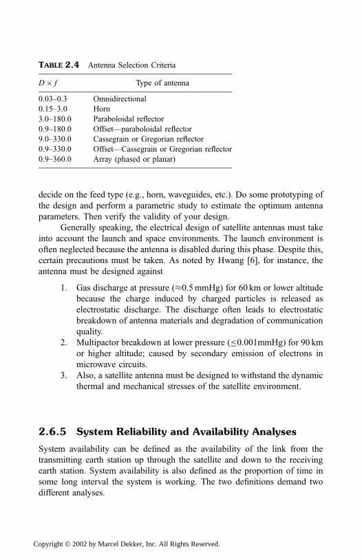
decide on the feed type (e.g., horn, waveguides, etc.). Do some prototyping of
the design and perform a parametric study to estimate the optimum antenna
parameters. Then verify the validity of your design.
Generally speaking, the electrical design of satellite antennas must take
into account the launch and space environments. The launch environment is
often neglected because the antenna is disabled during this phase. Despite this,
certain precautions must be taken. As noted by Hwang [6], for instance, the
antenna must be designed against
1. Gas discharge at pressure (0.5mmHg) for 60 km or lower altitude
because the charge induced by charged particles is released as
electrostatic discharge. The discharge often leads to electrostatic
breakdown of antenna materials and degradation of communication
quality.
2. Multipactor breakdown at lower pressure ( 0.001mmHg) for 90 km
or higher altitude; caused by secondary emission of electrons in
microwave circuits.
3. Also, a satellite antenna must be designed to withstand the dynamic
thermal and mechanical stresses of the satellite environment.
2.6.5 System Reliability and Availability Analyses
System availability can be defined as the availability of the link from the
transmitting earth station up through the satellite and down to the receiving
earth station. System availability is also defined as the proportion of time in
some long interval the system is working. The two definitions demand two
different analyses.
TABLE 2.4 Antenna Selection Criteria
D� f Type of antenna
0.03–0.3 Omnidirectional
0.15–3.0 Horn
3.0–180.0 Paraboloidal reflector
0.9–180.0 Offset—paraboloidal reflector
9.0–330.0 Cassegrain or Gregorian reflector
0.9–330.0 Offset—Cassegrain or Gregorian reflector
0.9–360.0 Array (phased or planar)
Copyright © 2002 by Marcel Dekker, Inc. All Rights Reserved.
By the first definition, the system availability expression can be
established by assuming that the system is made up of independently operating
subsystems—the transmitting earth station, the receiving earth station, and the
satellite. As such, a link outage, an earth station failure, and a satellite failure
occur mutually independently. The system engineer must first determine the
link availability, PLA, which is the average probability of the bit error
exceeding the design threshold, Pth. This threshold is the sum of the uplink
and downlink threshold outages, neglecting joint threshold outages. If we let
P0 represent the total percentage of outages per year above the threshold, then
the system link availability can be expressed as
PLA ¼ 1� Po ð2:26Þ
Thus, the system availability is
PSA ¼ PESAPLAPSATPESB ð2:27Þ
where
PSA ¼ system availability.
PESA ¼ availability of transmitting earth station A.
PESB ¼ availability of receiving earth station B.
PSAT ¼ satellite availability.
By the second definition, the system availability expression can be established
by also assuming that the system is made up of independently operating
subsystems—the transmitting earth station, the receiving earth station, and the
satellite. These subsystems fail independently and with adequate facilities to
initiate repair of any subsystem when it fails. The failure and repair process of
each subsystem is such that each subsystem can be associated with an up time,
a down time, and a time between failures which all have a constant mean value
when the system has been operating long enough to be in statistical
equilibrium. Then the means of these times can be denoted respectively by
MUT, MDT, and MTBF. This analysis assumes that
1. The system associated times depend on external events (e.g., rain-
ing, not raining, daytime, nighttime, eclipse, solar flare).
2. The means of these times can be defined for these events.
3. Online replacement of failed units by functioning units is in place.
Copyright © 2002 by Marcel Dekker, Inc. All Rights Reserved.
Then the system availability can be expressed as
PSA ¼MUT
MTBF
¼ MTBF�MDT
MTBF
ð2:28Þ
Similarly, the system unavailability can be written as
�PPSA ¼ 1� PSA
¼ MDT
MTBF
ð2:29Þ
The system reliability block diagram can be drawn, as in Fig. 2.10, for satellite
communication between two earth stations (A and B) to be established.
The system availability can be expressed as a product of each subsys-
tem’s availability:
PSA ¼MUTESA
MTBFESA
� �MUTSAT
MTBFSAT
� �MUTESB
MTBFESB
� �ð2:30Þ
Subscripts ESA, SAT, and ESB respectively denote earth station A, satellite,
and earth station B. If r of n units X1, X2, X3; . . . ;Xn are required for each
subsystem to be working, and each unit Xi has the same availability Pai; thenthe subsystem availability can be written as
PAsub ¼n
r
� �Prai�PPn�rai þ
n
r þ 1
� �Prþ1ai
�PPn�r�1ai þ � � �
þ n
r þ j
� �P
rþjai
�PPn�r�jai þ � � � þ Pn
ai ð2:31Þ
where ðn=mÞ are the binomial coefficients.
Example 2.2: The mean times per year of the earth stations A and B and the
satellite are collated as tabulated below. Calculate the system availability.
FIGURE 2.10 System reliability block diagram.
Copyright © 2002 by Marcel Dekker, Inc. All Rights Reserved.
Solution
From (2.28), we can estimate the availability of each subsystem:
Earth station A PaA ¼300� 3
300¼ 0:99
Earth station B PaB ¼200� 10
200¼ 0:95
Satellite PaSAT ¼500� 4
500¼ 0:992
Hence, the system availability from (2.30) is
PSA ¼ PaAPaBPaSAT ¼ 0:933
This means that the system will be available for 93.3% (alternatively,
unavailable for about 6.7%) of the year.
System Reliability
System reliability attempts to predict the future or quantitatively provides a
certain level of guarantees the system would meet; it is a by-product of
reliability theory. By definition, the reliability RðtÞ of a subsystem is the ratio
of the number of surviving components NsðtÞ within a system at time t to the
number of components at the start of the subsystem test period N0; that is,
RðtÞ ¼ NsðtÞN0
ð2:32Þ
The number of components that failed at time t can be written as
Nf ðtÞ ¼ N0 � NsðtÞ ð2:33Þ
From a system engineering perspective, we can relate any component failure to
the system MTBF. To do this, we need to know the probability of any one of
the components failing at the start. If one assumes that all components were
continuously tested until all of them failed, the MTBF of the ith component
failing after time ti can be written as
MTBF ¼ 1
N0
PN0
i¼1ti ð2:34Þ
Copyright © 2002 by Marcel Dekker, Inc. All Rights Reserved.
In fact, MTBF is the reciprocal of the average failure rate lr. For simplicity, the
average failure rate is assumed constant for a given batch of components.
Thus, for a small sample of failed components, we can write
lr ¼1
Ns
DNf
Dt¼ 1
Ns
dNf
dtð2:35Þ
Alternatively, lr can be expressed in terms of the rate of survival (dNs=dt) asfollows. Differentiating (2.33) with respect to t, we found that dNs=dt is thenegative of dNf =dt. By substituting the differentiation in (2.35) and in view of
the reliability definition of (2.32), the average failure rate is
lr ¼ �1
Ns
dNs
dt
¼ � 1
RðtÞdRðtÞdt
ð2:36Þ
A solution for reliability RðtÞ in (2.36) may be written as
RðtÞ ¼ e�lr t ð2:37Þ
This expression shows that reliability decreases exponentially with time, with
zero reliability after infinite time (t � 1). In practice, the end of useful life is
often taken to be the time t at which reliability falls to 0.3679 (i.e., 1=e), whichis when t ¼ MTBF. An example of a reliability problem is given in Sec. 2.8
(Example 2.6).
Redundancy
Redundancy is provided whenever failure of a unit or subsystem will cause the
loss of a significant part of the satellite communication capacity. A transponder
shown in Fig. 2.2, for example, will have two parallel pairs of a low-noise
amplifier (LNA) in the receive chain and two parallel pairs of a high-power
amplifier (HPA) in the transmit chain, as in Fig. 2.11. If one LNA is lost, the
transmitted signals from the antenna that pass through the LNA would be
recombined at the output of the other parallel LNA to avoid catastrophe.
Similarly, if one HPA is defective, the other HPA will allow information to be
transmitted.
Copyright © 2002 by Marcel Dekker, Inc. All Rights Reserved.
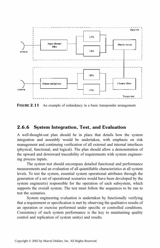
2.6.6 System Integration, Test, and Evaluation
A well-thought-out plan should be in place that details how the system
integration and assembly would be undertaken, with emphasis on risk
management and continuing verification of all external and internal interfaces
(physical, functional, and logical). The plan should allow a demonstration of
the upward and downward traceability of requirements with system engineer-
ing process inputs.
The system test should encompass detailed functional and performance
measurements and an evaluation of all quantifiable characteristics at all system
levels. To test the system, essential system operational attributes through the
generation of a set of operational scenarios would have been developed by the
system engineer(s) responsible for the operation of each subsystem, which
supports the overall system. The test must follow the sequences to be run to
test the scenarios.
System engineering evaluation is undertaken by functionally verifying
that a requirement or specification is met by observing the qualitative results of
an operation or exercise performed under specific or controlled conditions.
Consistency of such system performance is the key to maintaining quality
control and replication of system unit(s) and results.
FIGURE 2.11 An example of redundancy in a basic transponder arrangement.
Copyright © 2002 by Marcel Dekker, Inc. All Rights Reserved.
2.7 ANTENNAS
Based on function, satellite antennas can be classified into the following
categories: communication and special satellite antennas [8]. The commu-
nication antennas are used for tracking, telemetry, and command operation
throughout mission phases after launch vehicle separation. A nondirectional
(i.e., omnidirectional) and circularly polarized antenna is required to ensure
the continuous coverage and reception of command signals during mission
operation. Two or more broadbeam antennas with switches can be used,
instead of a directional antenna, to provide continuous coverage. Special
satellite antennas, on the other hand, are directional for specific purposes, such
as meteorology, cross-link, earth coverage, and autotracking.
Simplistically, an antenna is the interface between a free-space electro-
magnetic wave and a guided wave. There are many types of antennas and
many different variations on the basic types, but their mode of operation is
essentially the same. That is, a radiofrequency transmitter excites electric
currents in the conductive surface layers of the antenna and radiates an
electromagnetic wave. If the same antenna is used with a receiver, the converse
process applies; that is, an incident radiowave excites currents in the antenna,
which are conducted to the receiver. The ability of an antenna to work both
ways is termed the principle of reciprocity.
An antenna’s radiation varies from omnidirectional to highly directional
and can be fixed or changed to accommodate specific needs as they arise.
Three basic, generic types of antennas are the reflector, lens, and phased
array; however, helical antennas have been deployed in space, particularly for
military systems.
A reflector antenna is the most desirable candidate for satellite antennas
because of its light weight, structural simplicity, and design maturity. Horns
are frequently used as feeds to illuminate reflector antennas, which typically
provide narrow beams. A horn antenna can be used alone, usually for wide-
angle coverage of the earth. The reflector, however, may need to be offset for
multiple-beam antenna systems to avoid feed blockage. The blockage destroys
the rotational symmetry of the surface and limits the range scan before
aberrations seriously degrade the scanning performance.
A lens antenna is the counterpart of the reflector from the optical
property point of view. It can be made rotationally symmetric to preserve good
optical characteristics. It has no feed blockage and compactness; however, it is
heavier at low-frequency applications and has lens surface mismatch.
A phased-array antenna is a class of array antennas that provides beam
agility by effecting a progressive change of phase between successive
Copyright © 2002 by Marcel Dekker, Inc. All Rights Reserved.
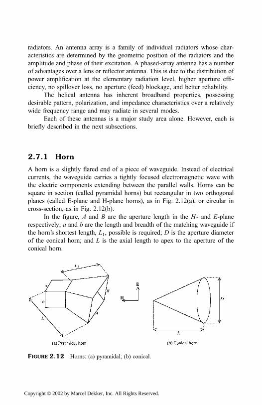
radiators. An antenna array is a family of individual radiators whose char-
acteristics are determined by the geometric position of the radiators and the
amplitude and phase of their excitation. A phased-array antenna has a number
of advantages over a lens or reflector antenna. This is due to the distribution of
power amplification at the elementary radiation level, higher aperture effi-
ciency, no spillover loss, no aperture (feed) blockage, and better reliability.
The helical antenna has inherent broadband properties, possessing
desirable pattern, polarization, and impedance characteristics over a relatively
wide frequency range and may radiate in several modes.
Each of these antennas is a major study area alone. However, each is
briefly described in the next subsections.
2.7.1 Horn
A horn is a slightly flared end of a piece of waveguide. Instead of electrical
currents, the waveguide carries a tightly focused electromagnetic wave with
the electric components extending between the parallel walls. Horns can be
square in section (called pyramidal horns) but rectangular in two orthogonal
planes (called E-plane and H-plane horns), as in Fig. 2.12(a), or circular in
cross-section, as in Fig. 2.12(b).
In the figure, A and B are the aperture length in the H- and E-plane
respectively; a and b are the length and breadth of the matching waveguide if
the horn’s shortest length, L1, possible is required; D is the aperture diameter
of the conical horn; and L is the axial length to apex to the aperture of the
conical horn.
FIGURE 2.12 Horns: (a) pyramidal; (b) conical.
Copyright © 2002 by Marcel Dekker, Inc. All Rights Reserved.
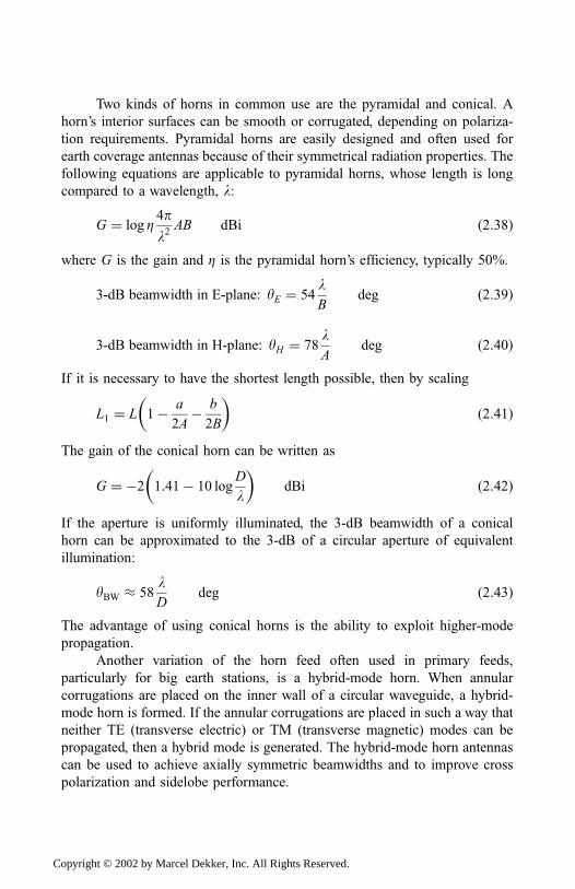
Two kinds of horns in common use are the pyramidal and conical. A
horn’s interior surfaces can be smooth or corrugated, depending on polariza-
tion requirements. Pyramidal horns are easily designed and often used for
earth coverage antennas because of their symmetrical radiation properties. The
following equations are applicable to pyramidal horns, whose length is long
compared to a wavelength, l:
G ¼ log Z4p
l2AB dBi ð2:38Þ
where G is the gain and Z is the pyramidal horn’s efficiency, typically 50%.
3-dB beamwidth in E-plane: yE ¼ 54lB
deg ð2:39Þ
3-dB beamwidth in H-plane: yH ¼ 78lA
deg ð2:40Þ
If it is necessary to have the shortest length possible, then by scaling
L1 ¼ L 1� a
2A� b
2B
� �ð2:41Þ
The gain of the conical horn can be written as
G ¼ �2 1:41� 10 logD
l
� �dBi ð2:42Þ
If the aperture is uniformly illuminated, the 3-dB beamwidth of a conical
horn can be approximated to the 3-dB of a circular aperture of equivalent
illumination:
yBW 58lD
deg ð2:43Þ
The advantage of using conical horns is the ability to exploit higher-mode
propagation.
Another variation of the horn feed often used in primary feeds,
particularly for big earth stations, is a hybrid-mode horn. When annular
corrugations are placed on the inner wall of a circular waveguide, a hybrid-
mode horn is formed. If the annular corrugations are placed in such a way that
neither TE (transverse electric) or TM (transverse magnetic) modes can be
propagated, then a hybrid mode is generated. The hybrid-mode horn antennas
can be used to achieve axially symmetric beamwidths and to improve cross
polarization and sidelobe performance.
Copyright © 2002 by Marcel Dekker, Inc. All Rights Reserved.
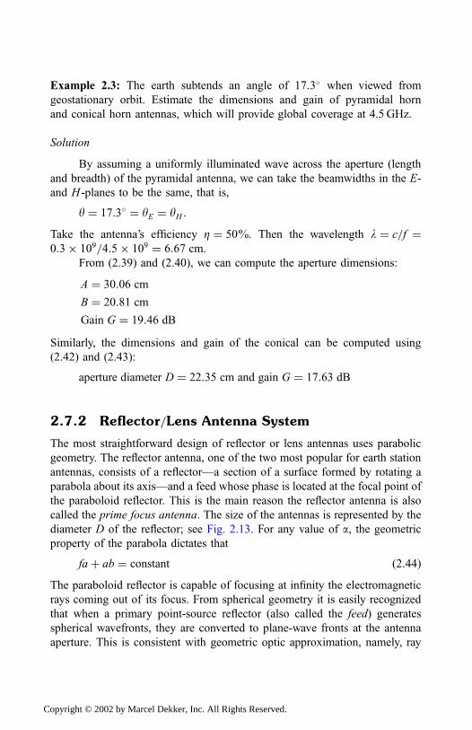
Example 2.3: The earth subtends an angle of 17:3� when viewed from
geostationary orbit. Estimate the dimensions and gain of pyramidal horn
and conical horn antennas, which will provide global coverage at 4.5GHz.
Solution
By assuming a uniformly illuminated wave across the aperture (length
and breadth) of the pyramidal antenna, we can take the beamwidths in the E-
and H-planes to be the same, that is,
y ¼ 17:3� ¼ yE ¼ yH :
Take the antenna’s efficiency Z ¼ 50%. Then the wavelength l ¼ c=f ¼0:3� 109=4:5� 109 ¼ 6:67 cm.
From (2.39) and (2.40), we can compute the aperture dimensions:
A ¼ 30:06 cm
B ¼ 20:81 cm
Gain G ¼ 19:46 dB
Similarly, the dimensions and gain of the conical can be computed using
(2.42) and (2.43):
aperture diameter D ¼ 22:35 cm and gain G ¼ 17:63 dB
2.7.2 Re£ector=Lens Antenna System
The most straightforward design of reflector or lens antennas uses parabolic
geometry. The reflector antenna, one of the two most popular for earth station
antennas, consists of a reflector—a section of a surface formed by rotating a
parabola about its axis—and a feed whose phase is located at the focal point of
the paraboloid reflector. This is the main reason the reflector antenna is also
called the prime focus antenna. The size of the antennas is represented by the
diameter D of the reflector; see Fig. 2.13. For any value of a, the geometric
property of the parabola dictates that
faþ ab ¼ constant ð2:44ÞThe paraboloid reflector is capable of focusing at infinity the electromagnetic
rays coming out of its focus. From spherical geometry it is easily recognized
that when a primary point-source reflector (also called the feed) generates
spherical wavefronts, they are converted to plane-wave fronts at the antenna
aperture. This is consistent with geometric optic approximation, namely, ray
Copyright © 2002 by Marcel Dekker, Inc. All Rights Reserved.
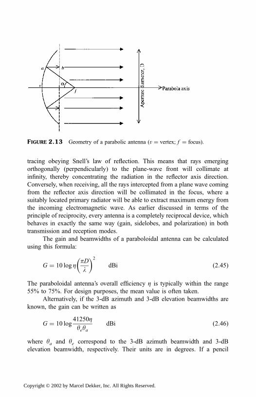
tracing obeying Snell’s law of reflection. This means that rays emerging
orthogonally (perpendicularly) to the plane-wave front will collimate at
infinity, thereby concentrating the radiation in the reflector axis direction.
Conversely, when receiving, all the rays intercepted from a plane wave coming
from the reflector axis direction will be collimated in the focus, where a
suitably located primary radiator will be able to extract maximum energy from
the incoming electromagnetic wave. As earlier discussed in terms of the
principle of reciprocity, every antenna is a completely reciprocal device, which
behaves in exactly the same way (gain, sidelobes, and polarization) in both
transmission and reception modes.
The gain and beamwidths of a paraboloidal antenna can be calculated
using this formula:
G ¼ 10 log ZpDl
� �2
dBi ð2:45Þ
The paraboloidal antenna’s overall efficiency Z is typically within the range
55% to 75%. For design purposes, the mean value is often taken.
Alternatively, if the 3-dB azimuth and 3-dB elevation beamwidths are
known, the gain can be written as
G ¼ 10 log41250Zyeya
dBi ð2:46Þ
where ya and ye correspond to the 3-dB azimuth beamwidth and 3-dB
elevation beamwidth, respectively. Their units are in degrees. If a pencil
FIGURE 2.13 Geometry of a parabolic antenna (v ¼ vertex; f ¼ focus).
Copyright © 2002 by Marcel Dekker, Inc. All Rights Reserved.
beam is assumed symmetrical (i.e., ya ¼ ye), then the 3-dB beamwidth can be
approximated using
ya 65l
DffiffiffiZp deg ð2:47Þ
Example 2.4: A paraboloidal antenna working at 1.8GHz and having a
diameter of 9.5m is required to achieve a gain of 41.5 dB. Find the necessary
efficiency. How much gain variation is associated with �4.5% efficiency
variation?
Solution
From (2.45) the antenna efficiency can be written in terms of other antenna
parameters:
Z ¼ 100:1GlpD
� �2
¼ 44:05%
So, for Z ¼ 44:05� 4:5%, we obtain gain G ¼ 41:5� 0:4 dB.
Re£ector=Lens Antenna Con¢guration
Many small paraboloidal antennas are front-fed; that is, the feed is situated at
the focus of the reflector, as shown in Fig. 2.14(a). However, the feeds of
transceiver earth station antennas may be bulky, especially if they transmit and
receive orthogonally polarized transmissions [8,9].
There are several variations to the basic parabolic configurations result-
ing in the creation of the Cassegrain antenna and the Gregorian antenna.
Cassegrain or Gregorian can be center-fed or offset. The center-fed arrange-
ments are shown in Fig. 2.14(b) and Fig. 2.14(c) for the Cassegrain and
Gregorian antenna, respectively. The antennas in Fig. 2.14 use main reflectors
whose surfaces are symmetrical about the axis of the paraboloid; hence the
name axisymmetric reflectors. The feeds of these antennas are at one focus of a
hyperboloidal subreflector while the other focus of the hyperboloidal is
coincident with the focus of the main reflector.
The advantage of using offset (asymmetric) reflectors is that the
subreflector can be put where it does not block or scatter the energy radiated
by, or falling on, the antenna aperture. By this arrangement, one can achieve
better sidelobe performance than the axisymmetric antennas.
The reflector or lens antenna can be configured to have single-feed or
multiple-feed elements. For the multiple-feed elements configuration, as in
Copyright © 2002 by Marcel Dekker, Inc. All Rights Reserved.
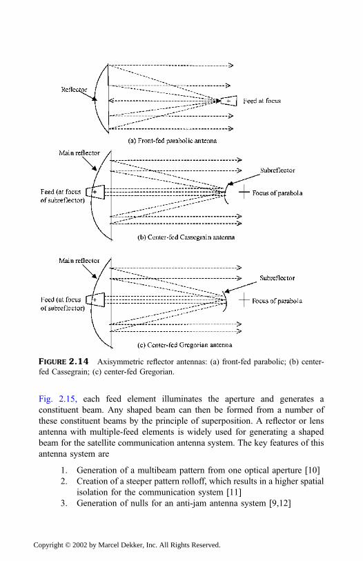
Fig. 2.15, each feed element illuminates the aperture and generates a
constituent beam. Any shaped beam can then be formed from a number of
these constituent beams by the principle of superposition. A reflector or lens
antenna with multiple-feed elements is widely used for generating a shaped
beam for the satellite communication antenna system. The key features of this
antenna system are
1. Generation of a multibeam pattern from one optical aperture [10]
2. Creation of a steeper pattern rolloff, which results in a higher spatial
isolation for the communication system [11]
3. Generation of nulls for an anti-jam antenna system [9,12]
FIGURE 2.14 Axisymmetric reflector antennas: (a) front-fed parabolic; (b) center-
fed Cassegrain; (c) center-fed Gregorian.
Copyright © 2002 by Marcel Dekker, Inc. All Rights Reserved.
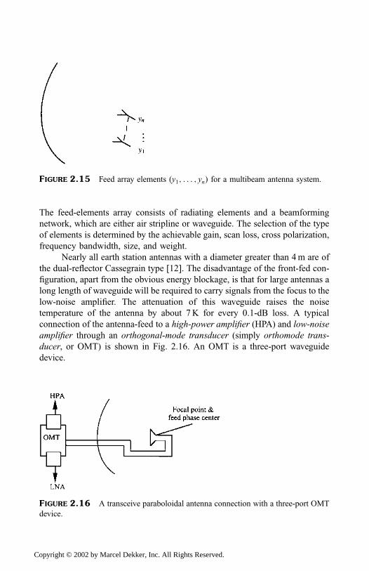
The feed-elements array consists of radiating elements and a beamforming
network, which are either air stripline or waveguide. The selection of the type
of elements is determined by the achievable gain, scan loss, cross polarization,
frequency bandwidth, size, and weight.
Nearly all earth station antennas with a diameter greater than 4m are of
the dual-reflector Cassegrain type [12]. The disadvantage of the front-fed con-
figuration, apart from the obvious energy blockage, is that for large antennas a
long length of waveguide will be required to carry signals from the focus to the
low-noise amplifier. The attenuation of this waveguide raises the noise
temperature of the antenna by about 7K for every 0.1-dB loss. A typical
connection of the antenna-feed to a high-power amplifier (HPA) and low-noise
amplifier through an orthogonal-mode transducer (simply orthomode trans-
ducer, or OMT) is shown in Fig. 2.16. An OMT is a three-port waveguide
device.
FIGURE 2.15 Feed array elements ðy1; . . . ; ynÞ for a multibeam antenna system.
FIGURE 2.16 A transceive paraboloidal antenna connection with a three-port OMT
device.
Copyright © 2002 by Marcel Dekker, Inc. All Rights Reserved.
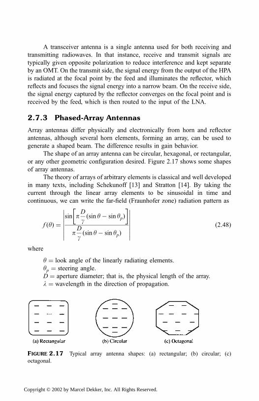
A transceiver antenna is a single antenna used for both receiving and
transmitting radiowaves. In that instance, receive and transmit signals are
typically given opposite polarization to reduce interference and kept separate
by an OMT. On the transmit side, the signal energy from the output of the HPA
is radiated at the focal point by the feed and illuminates the reflector, which
reflects and focuses the signal energy into a narrow beam. On the receive side,
the signal energy captured by the reflector converges on the focal point and is
received by the feed, which is then routed to the input of the LNA.
2.7.3 Phased-Array Antennas
Array antennas differ physically and electronically from horn and reflector
antennas, although several horn elements, forming an array, can be used to
generate a shaped beam. The difference results in gain behavior.
The shape of an array antenna can be circular, hexagonal, or rectangular,
or any other geometric configuration desired. Figure 2.17 shows some shapes
of array antennas.
The theory of arrays of arbitrary elements is classical and well developed
in many texts, including Schekunoff [13] and Stratton [14]. By taking the
current through the linear array elements to be sinusoidal in time and
continuous, we can write the far-field (Fraunhofer zone) radiation pattern as
f ðyÞ ¼sin p
D
gðsin y� sin ypÞ
� �pD
gðsin y� sin ypÞ
��������
�������� ð2:48Þ
where
y ¼ look angle of the linearly radiating elements.
yp ¼ steering angle.
D ¼ aperture diameter; that is, the physical length of the array.
l ¼ wavelength in the direction of propagation.
FIGURE 2.17 Typical array antenna shapes: (a) rectangular; (b) circular; (c)
octagonal.
Copyright © 2002 by Marcel Dekker, Inc. All Rights Reserved.
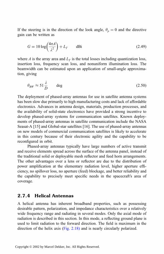
If the steering is in the direction of the look angle, yp ¼ 0 and the directive
gain can be written as
G ¼ 10 log4pA
l2
� �þ LT dBi ð2:49Þ
where A is the array area and LT is the total losses including quantization loss,
insertion loss, frequency scan loss, and nonuniform illumination loss. The
beamwidth can be estimated upon an application of small-angle approxima-
tion, giving
yBW 51lD
deg ð2:50Þ
The deployment of phased-array antennas for use in satellite antenna systems
has been slow due primarily to high manufacturing costs and lack of affordable
electronics. Advances in antenna design, materials, production processes, and
the availability of solid-state electronics have provided a strong incentive to
develop phased-array systems for communication satellites. Known deploy-
ments of phased-array antennas in satellite communication include the NASA
Seasat-A [15] and Global-star satellites [16]. The use of phased-array antennas
on new models of commercial communication satellites is likely to accelerate
in this century because of their electronic agility and the capability to be
reconfigured in orbit.
Phased-array antennas typically have large numbers of active transmit
and receive elements spread across the surface of the antenna panel, instead of
the traditional solid or deployable mesh reflector and feed horn arrangements.
The other advantages over a lens or reflector are due to the distribution of
power amplification at the elementary radiation level, higher aperture effi-
ciency, no spillover loss, no aperture (feed) blockage, and better reliability and
the capability to precisely meet specific needs in the spacecraft’s area of
coverage.
2.7.4 Helical Antennas
A helical antenna has inherent broadband properties, such as possessing
desirable pattern, polarization, and impedance characteristics over a relatively
wide frequency range and radiating in several modes. Only the axial mode of
radiation is described in this section. In this mode, a reflecting ground plane is
used to limit radiation to the forward direction. The field is maximum in the
direction of the helix axis (Fig. 2.18) and is nearly circularly polarized.
Copyright © 2002 by Marcel Dekker, Inc. All Rights Reserved.
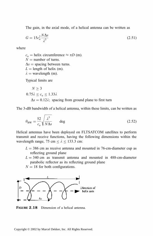
The gain, in the axial mode, of a helical antenna can be written as
G ¼ 15c2uNDs
l3ð2:51Þ
where
cu ¼ helix circumference pD (m).
N ¼ number of turns.
Ds ¼ spacing between turns.
L ¼ length of helix (m).
l ¼ wavelength (m).
Typical limits are
N � 3
0:75l cu 1:33l
Ds ¼ 0:12l; spacing from ground plane to first turn
The 3-dB bandwidth of a helical antenna, within these limits, can be written as
yBW ¼52
cu
ffiffiffiffiffiffiffiffiffil3
NDs
sdeg ð2:52Þ
Helical antennas have been deployed on FLTSATCOM satellites to perform
transmit and receive functions, having the following dimensions within the
wavelength range, 75 cm l 133:3 cm:
L ¼ 386 cm as receive antenna and mounted in 76-cm-diameter cup as
reflecting ground plane
L ¼ 340 cm as transmit antenna and mounted in 488-cm-diameter
parabolic reflector as its reflecting ground plane
N ¼ 18 for both configurations.
FIGURE 2.18 Dimension of a helical antenna.
Copyright © 2002 by Marcel Dekker, Inc. All Rights Reserved.
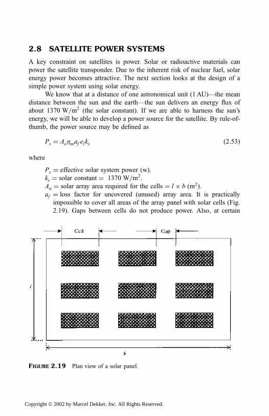
2.8 SATELLITE POWER SYSTEMS
A key constraint on satellites is power. Solar or radioactive materials can
power the satellite transponder. Due to the inherent risk of nuclear fuel, solar
energy power becomes attractive. The next section looks at the design of a
simple power system using solar energy.
We know that at a distance of one astronomical unit (1AU)—the mean
distance between the sun and the earth—the sun delivers an energy flux of
about 1370 W=m2 (the solar constant). If we are able to harness the sun’s
energy, we will be able to develop a power source for the satellite. By rule-of-
thumb, the power source may be defined as
Ps ¼ AaZmaf elks ð2:53Þ
where
Ps ¼ effective solar system power (w).
ks ¼ solar constant ¼ 1370 W=m2.
Aa ¼ solar array area required for the cells ¼ l � b ðm2Þ.af ¼ loss factor for uncovered (unused) array area. It is practically
impossible to cover all areas of the array panel with solar cells (Fig.
2.19). Gaps between cells do not produce power. Also, at certain
FIGURE 2.19 Plan view of a solar panel.
Copyright © 2002 by Marcel Dekker, Inc. All Rights Reserved.
angles, spacecraft may shadow the sun, hence this loss factor
estimation. A good estimate is about 20% for this loss factor.
el ¼ electrical losses, which account for losses in panel wiring, and
transmission losses in the cell cover glasses. A good estimate is about
20% for electrical losses.
Zm ¼ solar cells’ conversion efficiency; depends on the material used.
For example:
Zm ¼ 26% for gallium arsenide (GaAs) semiconductor.
Zm ¼ 23% for monocrystalline silicon.
Zm ¼ 10% for polycrystalline silicon.
The system designer may choose which material to use that will deliver the
required power to the system. Research studies are continuing to increase the
amount of sunlight solar cells that can be harnessed to about 37% to 40% of
the sun’s energy. Advanced flywheel technology could provide longer life for
power systems and more compact energy storage than chemical battery
systems.
During eclipses, solar cells are inert. To keep the communication system
operating, backup batteries make up the power system.
Example 2.5: A customer requires 140W of continuous power for a commu-
nication satellite. Design a power source that meets this requirement.
Solution
You are given P ¼ 140 W and solar constant kS ¼ 1370 W=m2.
You are at liberty to make sensible assumptions such as
1. Cell material efficiency Zm ¼ say, gallium arsenide (GaAs) semi-
conductor, Zm ¼ 26%.
2. Electrical loss factor el ¼ 20%.
3. Poorly arranged solar cells leave gaps af uncovered to 20% of
total area.
Hence, from (2.53), you require a panel of nominal area Aa ¼ 9:825 m2.
Example 2.6: A three-array arrangement of solar cells forms the power system
of a satellite system. The solar cells are connected in a series=parallel pattern,similar to that shown in Fig. 2.19. Preliminary tests indicate that each of the
three arrays, with each array having 80 cells, has the following failure rates:
Short-circuit failures in 108 hours
Nine open circuit failures in 108 hours
Copyright © 2002 by Marcel Dekker, Inc. All Rights Reserved.
Calculate (1) the probability that one solar cell goes (a) short-circuit and (b)
open circuit in a one-year period, (2) the probability that the three cells in one
arm short-circuit, and (3) the reliability of the solar power system for a one-
year period.
Solution
The solution to Example 2.5 uses the equations derived in (2.32)
through (2.36). So
Ns ¼ 80
dNf ¼ 6 for short-circuit
dNf ¼ 9 for open circuit
dt ¼ 108 hr
t ¼ ð365� 24Þ ¼ 8760 hr for nonleap year
1. To obtain the probability of the open and short-circuit cases, each
case’s failure rate and reliability must be established since their
probability P ¼ 1� reliability. Hence for
(a) A short-circuit cell, using (2.35) the average failure rate is
given by
lrðs=cÞ ¼1
Ns
dNf
dt¼ 1
80
6
108¼ 0:75*10�9
Using (2.37), the reliability is
R ¼ e�lrðs=cÞt ¼ 0:99999343
Hence, the probability of a short circuit within a calendar year
is
Ps=c ¼ 1� Rs=c ¼ 6:75*10�6
(b) Similarly, for an open circuit cell
lrðo=cÞ ¼1
Ns
dNf
dt¼ 1
80
9
108¼ 1:13*10�9
Its reliability Ro=c ¼ 0:99999015. The probability of an open
circuit within the calendar year Po=c ¼ 9:85*10�6.2. The probability of the cells array in one arm short-circuiting is
Parray ¼ Ns*Ps=c ¼ 80*6:57*10�6 ¼ 5:26*10�4
Copyright © 2002 by Marcel Dekker, Inc. All Rights Reserved.
3. The probability of both parallel arms short-circuiting is
Psystem ¼ 2*ðPs=cÞ3 ¼ 80*6:57*10�6 ¼ 5:26*10�4
Consequently, the reliability of the solar power system over a one-year period
is unity, or 100%.
2.9 ONBOARD PROCESSING AND SWITCHINGSYSTEMS
New-generation satellite technology requires more sophisticated processing of
carrier signals at the satellite prior to retransmission: an area referred to as
onboard processing. With this processing capability, a more efficient overall
satellite link can be realized, and it could lead to a simplification of the present
earth stations’ requirements. As stated in the introductory section of this
chapter, onboard processing enables the satellite to condition, amplify, or
reformat received uplink data and route (or switch) the data to specified
locations, or actually regenerate data onboard the spacecraft. The onboard
processor can provide a data storage facility required for a switched-beam
system and can also perform error correction on uplink data. A satellite system
that performs onboard processing is called a regenerative satellite.
Onboard processing is divided roughly into two parts: carrier proces-
sing and baseband processing. The basic concept of the carrier processing
technique is where the uplink modulated carriers from different sources are
distributed directly to output port (downlink) antennas using fixed or reconfi-
gurable (solid-state) circuitry and switches at the satellite; see Fig. 2.20. A
switch is reconfigurable when the interconnection patterns among its input and
output ports (channel filters) can be changed in response to changing patterns
among source–destination pairs. By this technique, no attempt is made to
recover the baseband data during the processing, and no changes in modula-
tion formats are allowed.
In baseband processing, the uplink carriers are first demodulated to
baseband data bits (or packets), then demultiplexed, switched (routed),
remodulated, and remultiplexed for delivery, each to a destination in different
downlink antennas. A schematic diagram of a baseband processor is shown in
Fig. 2.21. Multiplexing is the ability for multiple users to access a single
transponder circuit, also known as the process of combining separate signal
channels into one composite stream.
Multiplexing may be done in the time division mode, in which the
identity of each source of information is maintained by assigning that
Copyright © 2002 by Marcel Dekker, Inc. All Rights Reserved.
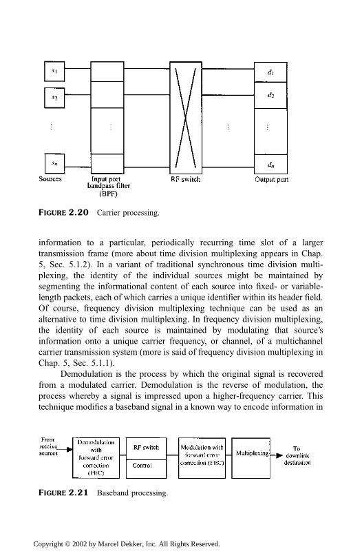
information to a particular, periodically recurring time slot of a larger
transmission frame (more about time division multiplexing appears in Chap.
5, Sec. 5.1.2). In a variant of traditional synchronous time division multi-
plexing, the identity of the individual sources might be maintained by
segmenting the informational content of each source into fixed- or variable-
length packets, each of which carries a unique identifier within its header field.
Of course, frequency division multiplexing technique can be used as an
alternative to time division multiplexing. In frequency division multiplexing,
the identity of each source is maintained by modulating that source’s
information onto a unique carrier frequency, or channel, of a multichannel
carrier transmission system (more is said of frequency division multiplexing in
Chap. 5, Sec. 5.1.1).
Demodulation is the process by which the original signal is recovered
from a modulated carrier. Demodulation is the reverse of modulation, the
process whereby a signal is impressed upon a higher-frequency carrier. This
technique modifies a baseband signal in a known way to encode information in
FIGURE 2.21 Baseband processing.
FIGURE 2.20 Carrier processing.
Copyright © 2002 by Marcel Dekker, Inc. All Rights Reserved.
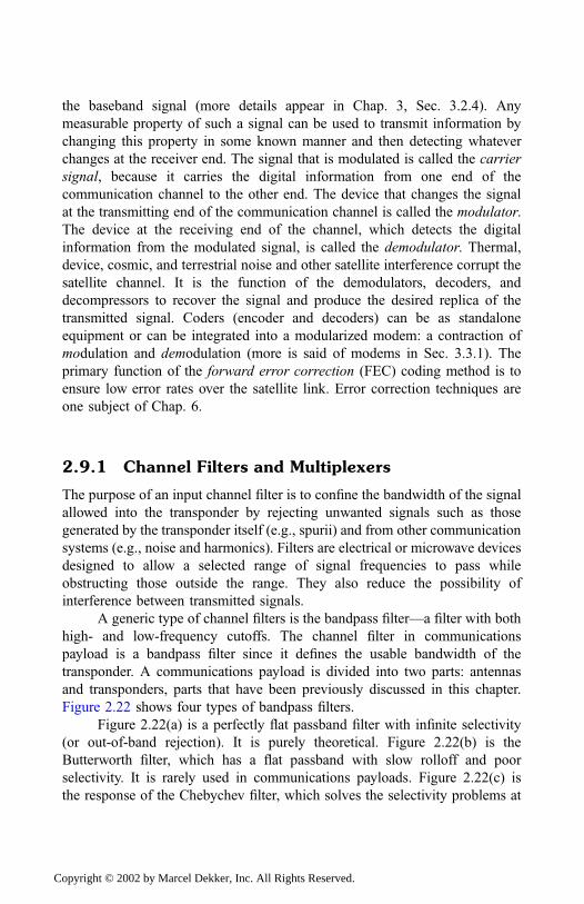
the baseband signal (more details appear in Chap. 3, Sec. 3.2.4). Any
measurable property of such a signal can be used to transmit information by
changing this property in some known manner and then detecting whatever
changes at the receiver end. The signal that is modulated is called the carrier
signal, because it carries the digital information from one end of the
communication channel to the other end. The device that changes the signal
at the transmitting end of the communication channel is called the modulator.
The device at the receiving end of the channel, which detects the digital
information from the modulated signal, is called the demodulator. Thermal,
device, cosmic, and terrestrial noise and other satellite interference corrupt the
satellite channel. It is the function of the demodulators, decoders, and
decompressors to recover the signal and produce the desired replica of the
transmitted signal. Coders (encoder and decoders) can be as standalone
equipment or can be integrated into a modularized modem: a contraction of
modulation and demodulation (more is said of modems in Sec. 3.3.1). The
primary function of the forward error correction (FEC) coding method is to
ensure low error rates over the satellite link. Error correction techniques are
one subject of Chap. 6.
2.9.1 Channel Filters and Multiplexers
The purpose of an input channel filter is to confine the bandwidth of the signal
allowed into the transponder by rejecting unwanted signals such as those
generated by the transponder itself (e.g., spurii) and from other communication
systems (e.g., noise and harmonics). Filters are electrical or microwave devices
designed to allow a selected range of signal frequencies to pass while
obstructing those outside the range. They also reduce the possibility of
interference between transmitted signals.
A generic type of channel filters is the bandpass filter—a filter with both
high- and low-frequency cutoffs. The channel filter in communications
payload is a bandpass filter since it defines the usable bandwidth of the
transponder. A communications payload is divided into two parts: antennas
and transponders, parts that have been previously discussed in this chapter.
Figure 2.22 shows four types of bandpass filters.
Figure 2.22(a) is a perfectly flat passband filter with infinite selectivity
(or out-of-band rejection). It is purely theoretical. Figure 2.22(b) is the
Butterworth filter, which has a flat passband with slow rolloff and poor
selectivity. It is rarely used in communications payloads. Figure 2.22(c) is
the response of the Chebychev filter, which solves the selectivity problems at
Copyright © 2002 by Marcel Dekker, Inc. All Rights Reserved.
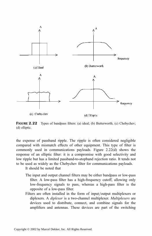
the expense of passband ripple. The ripple is often considered negligible
compared with mismatch effects of other equipment. This type of filter is
commonly used in communications payloads. Figure 2.22(d) shows the
response of an elliptic filter: it is a compromise with good selectivity and
low ripple but has a limited passband-to-stopband rejection ratio. It tends not
to be used as widely as the Chebychev filter for communications payloads.
It should be noted that
The input and output channel filters may be either bandpass or low-pass
filter. A low-pass filter has a high-frequency cutoff, allowing only
low-frequency signals to pass, whereas a high-pass filter is the
opposite of a low-pass filter.
Filters are often installed in the form of input=output multiplexers or
diplexers. A diplexer is a two-channel multiplexer. Multiplexers are
devices used to distribute, connect, and combine signals for the
amplifiers and antennas. These devices are part of the switching
FIGURE 2.22 Types of bandpass filters: (a) ideal; (b) Butterworth; (c) Chebychev;
(d) elliptic.
Copyright © 2002 by Marcel Dekker, Inc. All Rights Reserved.
matrix in the communications subsystem of a satellite. In fact, a
multiplexer is a multichannel filter. For instance, where a number of
channels share the bandwidth available in a satellite transponder, an
input multiplexer separates the channel frequencies and routes each
carrier to its own amplifier chain. Once amplified, the channels are
recombined in an output multiplexer for return transmission.
The channel output filter has a narrower passband than the input filter. It
is this output channel filter that defines the usable bandwidth of the
transponder—an important quantity as far as the service’s user is
concerned.
2.9.2 Other Onboard Communication Subsystems
For completeness, other components comprising the transponder, depicted in
block diagram in Fig. 2.2, are described in this section. The description
enriches the reader’s understanding of the overall satellite systems.
Low-Noise Ampli¢ers (LNA)
The design objective of the LNA is to deliver a good signal-to-noise ratio
(SNR). The reader will learn in Sec. 4.1 that the typical received signal power
is extremely low. As such, it is imperative to reject noise introduced in the
signal during its passage through the 36,000 km of free space. If the noise is
carried through the entire chain, it will be successively amplified and finally
retransmitted. Two types of LNA are frequently utilized: a bipolar transistor
used up to 2GHz and a field effect transistor (FET) used where the carrier
frequency is between 2 and 20GHz.
High-Power Ampli¢ers (HPA)
High-power amplifiers are traditionally travelling wave tube amplifiers
(TWTA). The function of the HPA is to provide the radiofrequency power
the downlink needs in order to maintain the required carrier-to-noise ratio,
ðC=N Þ at the earth terminals with minimum amplitude variation. The func-
tional relationship between the SNR and C=N will become clearer to the
reader in Chap. 3. TWTAs are part of a family of microwave tubes, which
includes magnetrons and klystrons. These tubes (magnetrons and klystrons)
permit frequency agility and in-pulse frequency scanning, which are essential
features of modern communication systems. Figure 2.23 shows a klystron.
Copyright © 2002 by Marcel Dekker, Inc. All Rights Reserved.
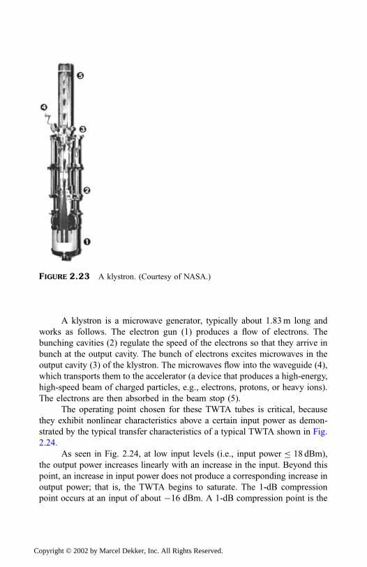
A klystron is a microwave generator, typically about 1.83m long and
works as follows. The electron gun (1) produces a flow of electrons. The
bunching cavities (2) regulate the speed of the electrons so that they arrive in
bunch at the output cavity. The bunch of electrons excites microwaves in the
output cavity (3) of the klystron. The microwaves flow into the waveguide (4),
which transports them to the accelerator (a device that produces a high-energy,
high-speed beam of charged particles, e.g., electrons, protons, or heavy ions).
The electrons are then absorbed in the beam stop (5).
The operating point chosen for these TWTA tubes is critical, because
they exhibit nonlinear characteristics above a certain input power as demon-
strated by the typical transfer characteristics of a typical TWTA shown in Fig.
2.24.
As seen in Fig. 2.24, at low input levels (i.e., input power 18 dBm),
the output power increases linearly with an increase in the input. Beyond this
point, an increase in input power does not produce a corresponding increase in
output power; that is, the TWTA begins to saturate. The 1-dB compression
point occurs at an input of about �16 dBm. A 1-dB compression point is the
FIGURE 2.23 A klystron. (Courtesy of NASA.)
Copyright © 2002 by Marcel Dekker, Inc. All Rights Reserved.
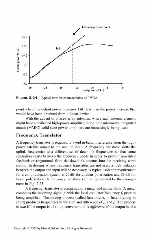
point where the output power increases 1 dB less than the power increase that
would have been obtained from a linear device.
With the advent of phased-array antennas, where each antenna element
might have a dedicated high-power amplifier, monolithic microwave integrated
circuit (MMIC) solid-state power amplifiers are increasingly being used.
Frequency Translator
A frequency translator is required to avoid in-band interference from the high-
power satellite output to the satellite input. A frequency translator shifts the
uplink frequencies to a different set of downlink frequencies so that some
separation exists between the frequency bands in order to prevent unwanted
feedback or ringaround, from the downlink antenna into the receiving earth
station. In designs where frequency translators are not used, a high isolation
between the output and input will be necessary. A typical isolation requirement
for a communication system is 27 dB for circular polarization and 33 dB for
linear polarization. A frequency translator can be represented by the arrange-
ment in Fig. 2.25.
A frequency translator is comprised of a mixer and an oscillator. A mixer
combines the incoming signal fc with the local oscillator frequency fl prior to
being amplified. The mixing process (called heterodyne, or heterodyning in
short) produces frequencies to the sum and difference of fc and fl. The process
is sum if the output is of an up converter and is difference if the output is of a
FIGURE 2.24 Typical transfer characteristics of TWTA.
Copyright © 2002 by Marcel Dekker, Inc. All Rights Reserved.
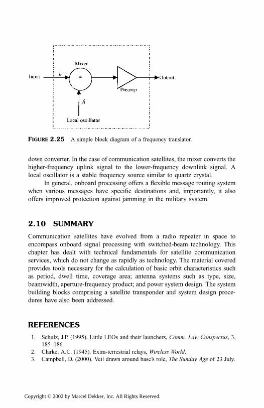
down converter. In the case of communication satellites, the mixer converts the
higher-frequency uplink signal to the lower-frequency downlink signal. A
local oscillator is a stable frequency source similar to quartz crystal.
In general, onboard processing offers a flexible message routing system
when various messages have specific destinations and, importantly, it also
offers improved protection against jamming in the military system.
2.10 SUMMARY
Communication satellites have evolved from a radio repeater in space to
encompass onboard signal processing with switched-beam technology. This
chapter has dealt with technical fundamentals for satellite communication
services, which do not change as rapidly as technology. The material covered
provides tools necessary for the calculation of basic orbit characteristics such
as period, dwell time, coverage area; antenna systems such as type, size,
beamwidth, aperture-frequency product; and power system design. The system
building blocks comprising a satellite transponder and system design proce-
dures have also been addressed.
REFERENCES
1. Schulz, J.P. (1995). Little LEOs and their launchers, Comm. Law Conspectus, 3,
185–186.
2. Clarke, A.C. (1945). Extra-terrestrial relays, Wireless World.
3. Campbell, D. (2000). Veil drawn around base’s role, The Sunday Age of 23 July.
FIGURE 2.25 A simple block diagram of a frequency translator.
Copyright © 2002 by Marcel Dekker, Inc. All Rights Reserved.
4. Iridium LCC (1997). Iridium System Facts.
http:==www.apspg.com=whatsnew=iridium=facts.html
5. Teledisic (1998). Technical overview of the Teledesic network.
http:==www.teledisic.com=tech=details.html
6. Porcelli, G. (1986). Effects of atmospheric refraction on sun interference, INTEL-
SAT Technical Memorandum, IOD-E-86-05.
7. Kitsuregawa, T. (1990). Advanced Technology in Satellite Communication
Antenna: Electrical and Mechanical Design. Artech House.
8. Mayhan, J.T. (1983). Adaptive antenna design considerations for satellite commu-
nication antennas, Proc. IEEE, 130, parts F & H.
9. Pritchard, W.L., Suyderhoud, H.G., and Nelson, R.A. (1993). Satellite Commu-
nication Systems Engineering. Prentice-Hall.
10. Hwang, Y. (1992). Satellite antennas, Proc. IEEE, 80, 183–193.
11. Dalgleish, D.I. (1989). An Introduction to Satellite Communications. Peter
Peregrinus.
12. Maral, G. and Bousquet, M. (1993). Satellite Communications System: Systems,
Techniques and Technology. John Wiley.
13. Schekunoff, S.A. (1943). Electromagnetic Waves. D van Nostrand.
14. Stratton, J.A. (1941). Electromagnetic Theory. McGraw-Hill.
15. Aviation Week & Space Technology, Dec. 1977, 51.
16. Aviation Week & Space Technology, Jan. 1999, 65.
PROBLEMS
1. A satellite system consists of 1000 units in series configuration. The failure
rate of each unit is 0.48% per 1000 hours and is known to be constant. If
the mission time of the system is 1000 hours, calculate the system
reliability. If the desired reliability of the system for a mission time of
1000 hours is 0.98, determine what failure rate would be required of the
components.
2. An earth station is located at 79:34�W longitude and 37:09�N latitude.
Calculate its look angle and range to a geosynchronous satellite whose
subsatellite point is located at 102�W longitude.
3. Your colleague has been told to design an earth station, which is to be
located in your town. As an independent observer, you are encouraged to
provide a solution to check your colleague’s calculation. The subsatellite
point should be within �22:25� of the town’s longitude. Write a computer
program to compute the various look angles and ranges to a satellite located
in geosynchronous orbit.
4. A customer required 165.85W continuous power for a communication
satellite. Design a power source that meets this requirement. What addi-
Copyright © 2002 by Marcel Dekker, Inc. All Rights Reserved.
tional protection is required to ensure continuity of supply during a partial
or total eclipse?
5. Given a satellite altitude and desired illumination spot diameter on the
earth’s surface, simulate the antenna aperture diameter and maximum gain
to give the desired spot diameter.
6. Briefly describe the usefulness of an antenna in satellite communication.
7. Describe how the capacity of a transmission channel can be measured.
Copyright © 2002 by Marcel Dekker, Inc. All Rights Reserved.
3
Earth Stations
In Chap. 2 we discuss the basic structure of a satellite system. We now
consider a vital part of the overall satellite system: earth stations. An earth
station is a collection of equipment for communicating with the satellite,
regardless of whether it is fixed, mobile, aeronautical, or marine terminals. An
earth station provides a means of transmitting the modulated RF carrier to the
satellite within the uplink frequency spectrum and receiving the RF carrier
from the satellite with the downlink frequency spectrum. It is the vital link
between satellites and communications users.
This chapter considers a basic arrangement of an earth station, the
technical and operational requirements, the different types of earth stations
used for day-to-day communications, the switching technique employed, the
system capacity requirements, and the interface with terrestrial equipment and
users.
Copyright © 2002 by Marcel Dekker, Inc. All Rights Reserved.
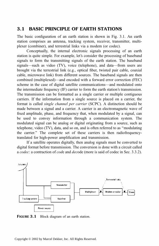
3.1 BASIC PRINCIPLE OF EARTH STATIONS
The basic configuration of an earth station is shown in Fig. 3.1. An earth
station comprises an antenna, tracking system, receiver, transmitter, multi-
plexer (combiner), and terrestrial links via a modem (or codec).
Conceptually, the internal electronic signals processing of an earth
station is quite simple. For example, let’s consider the processing of baseband
signals to form the transmitting signals of the earth station. The baseband
signals—such as video (TV), voice (telephone), and data—from users are
brought via the terrestrial link (e.g., optical fiber, twisted pair cable, coaxial
cable, microwave link) from different sources. The baseband signals are then
combined (multiplexed)—and encoded with a forward error correction (FEC)
scheme in the case of digital satellite communications—and modulated onto
the intermediate frequency (IF) carrier to form the earth station’s transmission.
The transmission can be formatted as a single carrier or multiple contiguous
carriers. If the information from a single source is placed on a carrier, the
format is called single channel per carrier (SCPC). A distinction should be
made between a signal and a carrier. A carrier is an electromagnetic wave of
fixed amplitude, phase, and frequency that, when modulated by a signal, can
be used to convey information through a communication system. The
modulated signal can be analog or digital originating from a source, such as
telephone, video (TV), data, and so on, and is often referred to as ‘‘modulating
the carrier.’’ The complete set of these carriers is then radiofrequency-
translated for high-power amplification and transmission.
If a satellite operates digitally, then analog signals must be converted to
digital format before transmission. The conversion is done with a circuit called
a codec: a contraction of code and decode (more is said of codec in Sec. 3.3.2).
FIGURE 3.1 Block diagram of an earth station.
Copyright © 2002 by Marcel Dekker, Inc. All Rights Reserved.
The most popular forms of modulation used in digital communications are
binary phase shift keying (BPSK), quadrature phase shift keying (QPSK),
offset-quadrature phase shift keying (OQPSK), and 8-PSK. These modulation
formats can be described in a general form as M-PSK modulation, where
M ¼ 2b bits, each symbol represents b bits, and b is an integer, 1, 2, or 3. The
generalized M-PSK is discussed in Sec. 3.2.
A modem converts a digital signal to an analog tone (modulation) and
reconverts the analog tone (demodulation) into its original digital signal at the
other side of connection (modems are described in Sec. 3.3.1). Both ampli-
tude-modulation (AM) and frequency-modulation (FM) techniques are exam-
ples of analog-type or uncoded signal-transmission systems with one-to-one
correspondence between the input signal and the modulated carrier eventually
transmitted.
The reader might ask, why code? A coded system makes much more
efficient use of bandwidth widening to increase the output signal-to-noise ratio
than does an uncoded system. Coded systems are inherently capable of better
transmission efficiency than the uncoded types.
A general division may be made to classify frequency division multi-
plexing (FDM) voice and video signals to use FM while classifying digitally
multiplexed voice and data to use some form of phase modulation.
In the receiving chain, the received signals pass through a sequence of
processing steps that are essentially the reverse of those followed to prepare
the outgoing signals. The RF received signals are passed through a low-noise
wideband RF front end, followed by a translator to IF. It is at the IF stage that
the specific uplink carriers hoping to be received are separated and grouped by
destination, then demodulated to their original baseband signals followed by
an FEC decoder (in the case of digital satellite communications). Those not
specifically destined to the earth station are retransmitted, thereby acting like a
transponder. The demodulated baseband signals may then be demultiplexed, if
necessary, and thereby transferred to the users.
The antenna in Fig. 3.1 is used for transmitting and receiving: this type
is called a transceiver. The basic principles and characteristics of antennas
have been discussed in Chap. 2, Sec. 2.7; they also apply to the earth station
antennas. However, in addition to the antenna characteristics discussed in Sec.
2.7, the antenna subsystem requires separate tracking equipment, which
ensures precise pointing of the antenna at the satellite. With small earth
stations where the antenna’s bandwidth is large, precision-tracking equipment
is not necessary. The antenna tracking system can be programmed to point to
preassigned direction(s) automatically and can also be directed manually. We
discuss more on antenna tracking systems in Sec. 3.4.2.
Copyright © 2002 by Marcel Dekker, Inc. All Rights Reserved.
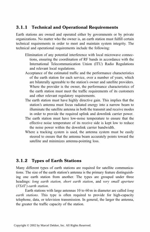
3.1.1 Technical and Operational Requirements
Earth stations are owned and operated either by governments or by private
organizations. No matter who the owner is, an earth station must fulfill certain
technical requirements in order to meet and maintain system integrity. The
technical and operational requirements include the following:
Elimination of any potential interference with local microwave connec-
tions, ensuring the coordination of RF bands in accordance with the
International Telecommunication Union (ITU) Radio Regulations
and relevant local regulations.
Acceptance of the estimated traffic and the performance characteristics
of the earth station for each service, over a number of years, which
are bilaterally agreeable to the station’s owner and satellite providers.
Where the provider is the owner, the performance characteristics of
the earth station must meet the traffic requirements of its customers
and other relevant regulatory requirements.
The earth station must have highly directive gain. This implies that the
station’s antenna must focus radiated energy into a narrow beam to
illuminate the satellite antenna in both the transmit and receive modes
in order to provide the required uplink and downlink carrier power.
The earth station must have low-noise temperature to ensure that the
effective noise temperature of its receive side is kept low to reduce
the noise power within the downlink carrier bandwidth.
Where a tracking system is used, the antenna system must be easily
steered to ensure that the antenna beam accurately points toward the
satellite and minimizes antenna-pointing loss.
3.1.2 Types of Earth Stations
Many different types of earth stations are required for satellite communica-
tions. The size of the earth station’s antenna is the primary feature distinguish-
ing one earth station from another. The types are grouped under three
headings: long earth station, short earth station, and very small aperture
ðVSAT Þ earth station.
Earth stations with large antennas 10 to 60m in diameter are called long
earth stations. This type is often required to provide for high-capacity
telephone, data, or television transmission. In general, the larger the antenna,
the greater the traffic capacity of the station.
Copyright © 2002 by Marcel Dekker, Inc. All Rights Reserved.
Small earth stations are antennas with diameters between 1 and 10m.
They are commonly sighted on the roofs or in the gardens of domestic and
commercial buildings. Small earth stations provide capabilities for reception
of broadcast television and=or connection for thin-route telephony systems in
remote regions.
Very small aperture (VSAT) earth stations are networks of satellite earth
terminals, each of which has an antenna diameter between 0.3 and 0.9m:
hence the name ‘‘very small.’’ VSAT networks are usually arranged in a star
configuration in which small aperture terminals each communicate via the
satellite to a large central earth station known as a hub station. Any aperture
smaller than VSAT is called an ultra-small aperture terminal (USAT ).
Nearly all earth station antennas with a diameter greater than 4m are of
the paraboloidal-reflector Cassegrain type (discussed in Chap. 2, Sec. 2.7.2)
with the following advantages [1]:
Greater electrical design flexibility, which allows aperture illumination
efficiency to be maximized
Feed is easily accessible and connectable to LNAs and HPAs
Primary spillover is normally directed toward clear sky, which picks less
noise than the conventional parabolic configurations
Operational flexibility, particularly in moving the antenna easily in either
azimuthal and elevation directions
3.2 MODULATION
Modulation is a signal processing technique that involves switching or keying
the amplitude, frequency, or phase of the carrier in accordance with the
information binary digits. There are three basic modulation schemes: ampli-
tude shift keying (ASK), frequency shift keying (FSK), and phase shift keying
(PSK). These schemes are, respectively, the binary equivalent of analog
transmission’s amplitude modulation (AM), frequency modulation (FM), and
pulse modulation (PM) when used to transmit data signals.
Consider an input signal sðtÞ of duration Ts represented by
sðtÞ ¼ A cosð2pfct þ fnÞ; ðn� 1ÞTs t nTs ð3:1Þwhere A and fn correspond to the amplitude and nth phase of the signal.
For the ASK scheme, the signal’s amplitude A is varied while the phase
fn and carrier frequency fc remain constant. In the FSK, only the frequency fcis varied, with A and fn remaining constant. In the case of PSK, A and fc are
kept constant, with the fn varied. PSK, compared with the other schemes, has
Copyright © 2002 by Marcel Dekker, Inc. All Rights Reserved.
excellent protection against noise because the information is contained within
its phase. Noise mainly affects the amplitude of the carrier.
In the M-PSK schemes, the phase of the carrier takes on one of M
possible values or symbols. The (stream of ) input binary data is first divided
into b-bit blocks. Each block is transmitted as one of M possible values or
symbols. Each symbol is a carrier frequency sinusoid having one of M
possible phase values spaced 2p=M apart. Then, for the nth M -tuple say,
the M-PSK phase of (3.1) will exist in all intervals:
fn 2 0;2pM
;4pM
; . . . ;2ðM � 1Þp
M
To ensure that each transmitted binary digit contains an integral number of
cycles, the unmodulated carrier frequency fc ¼ kc=Ts; where kc is a fixed
integer. For example, if the amplitude of (3.1) has a plus or minus unity value,
that is, A ¼ �1, then kc ¼ 2. A pair of signals that differ in phase by 180� isreferred to as antipodal signals.
For M-PSK, a symbol duration
Ts ¼ Tb log2 M
¼ bTb ð3:2Þ
providing there is no reduction in information throughput, where Tb is the
input binary interval.
From this M-PSK generalization, one can derive the most important
modulation schemes used in satellite communications: BPSK, QPSK or
OQPSK, and 8-PSK. The derivation is as follows.
3.2.1 Binary PSK
When the index b ¼ 1;M ¼ 2, a binary PSK is derived. It is also referred to as
BPSK or 2-PSK. In this case, the binary input baseband data vðtÞ modulates
constant amplitude, constant frequency in such a way that two phase values
differing by 180� (recall 2p=M , where M in this case is 2) represent the binary
symbols 0 and 1, respectively. The corresponding BPSK symbol expression
can be written as
sðtÞ ¼ AvðtÞ sinoct ð3:3ÞThe BPSK signal constellation (space) diagram is shown in Fig. 3.2, where I
and Q represent the in-phase and in-quadrature axes, respectively.
Copyright © 2002 by Marcel Dekker, Inc. All Rights Reserved.
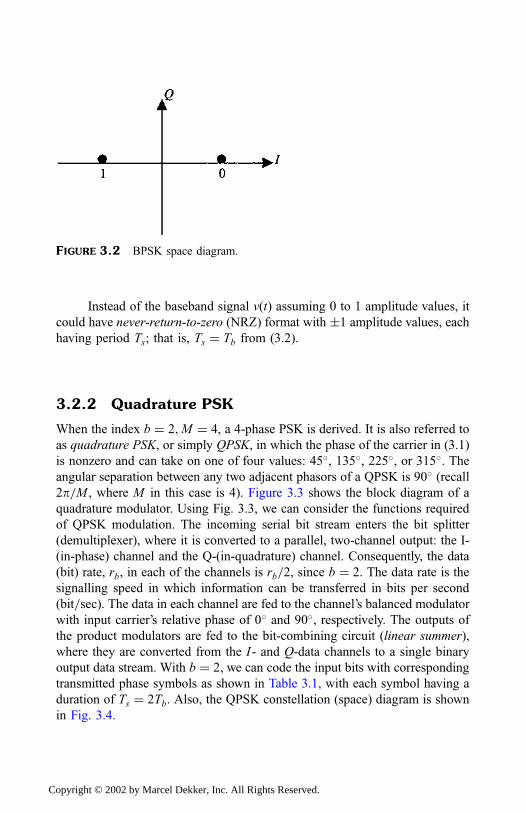
Instead of the baseband signal vðtÞ assuming 0 to 1 amplitude values, it
could have never-return-to-zero (NRZ) format with �1 amplitude values, each
having period Ts; that is, Ts ¼ Tb from (3.2).
3.2.2 Quadrature PSK
When the index b ¼ 2;M ¼ 4, a 4-phase PSK is derived. It is also referred to
as quadrature PSK, or simply QPSK, in which the phase of the carrier in (3.1)
is nonzero and can take on one of four values: 45�, 135�, 225�, or 315�. Theangular separation between any two adjacent phasors of a QPSK is 90� (recall2p=M , where M in this case is 4). Figure 3.3 shows the block diagram of a
quadrature modulator. Using Fig. 3.3, we can consider the functions required
of QPSK modulation. The incoming serial bit stream enters the bit splitter
(demultiplexer), where it is converted to a parallel, two-channel output: the I-
(in-phase) channel and the Q-(in-quadrature) channel. Consequently, the data
(bit) rate, rb, in each of the channels is rb=2, since b ¼ 2. The data rate is the
signalling speed in which information can be transferred in bits per second
(bit=sec). The data in each channel are fed to the channel’s balanced modulator
with input carrier’s relative phase of 0� and 90�, respectively. The outputs of
the product modulators are fed to the bit-combining circuit (linear summer),
where they are converted from the I - and Q-data channels to a single binary
output data stream. With b ¼ 2, we can code the input bits with corresponding
transmitted phase symbols as shown in Table 3.1, with each symbol having a
duration of Ts ¼ 2Tb. Also, the QPSK constellation (space) diagram is shown
in Fig. 3.4.
FIGURE 3.2 BPSK space diagram.
Copyright © 2002 by Marcel Dekker, Inc. All Rights Reserved.
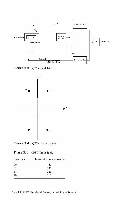
FIGURE 3.3 QPSK modulator.
FIGURE 3.4 QPSK space diagram.
TABLE 3.1 QPSK Truth Table
Input bits Transmitted phase symbol
00 45�
01 135�
11 225�
10 315�
Copyright © 2002 by Marcel Dekker, Inc. All Rights Reserved.
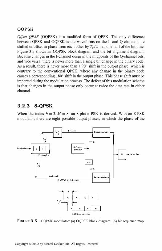
OQPSK
Offset QPSK (OQPSK) is a modified form of QPSK. The only difference
between QPSK and OQPSK is the waveforms on the I- and Q-channels are
shifted or offset in-phase from each other by Tb=2, i.e., one-half of the bit time.
Figure 3.5 shows an OQPSK block diagram and the bit alignment diagram.
Because changes in the I-channel occur in the midpoints of the Q-channel bits,
and vice versa, there is never more than a single bit change in the binary code.
As a result, there is never more than a 90� shift in the output phase, which is
contrary to the conventional QPSK, where any change in the binary code
causes a corresponding 180� shift in the output phase. This phase shift must be
imparted during the modulation process. The defect of this modulation scheme
is that changes in the output phase only occur at twice the data rate in either
channel.
3.2.3 8-QPSK
When the index b ¼ 3;M ¼ 8, an 8-phase PSK is derived. With an 8-PSK
modulator, there are eight possible output phases, in which the phase of the
FIGURE 3.5 OQPSK modulator: (a) OQPSK block diagram; (b) bit sequence map.
Copyright © 2002 by Marcel Dekker, Inc. All Rights Reserved.
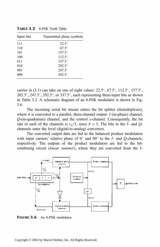
carrier in (3.1) can take on one of eight values: 22.5�, 67.5�, 112.5�, 157.5�,202.5�, 247.5�, 292.5�, or 337.5�, each representing three-input bits as shown
in Table 3.2. A schematic diagram of an 8-PSK modulator is shown in Fig.
3.6.
The incoming serial bit stream enters the bit splitter (demultiplexer),
where it is converted to a parallel, three-channel output: I -(in-phase) channel,
Q-(in-quadrature) channel, and the control x-channel. Consequently, the bit
rate in each of the channels is rb=3, since b ¼ 3. The bits in the I - and Q-
channels enter the level (digital-to-analog) converters.
The converted output data are fed to the balanced product modulators
with input carriers’ relative phase of 0� and 90� to the I - and Q-channels,
respectively. The outputs of the product modulators are fed to the bit-
combining circuit (linear summer), where they are converted from the I -
FIGURE 3.6 An 8-PSK modulator.
TABLE 3.2 8-PSK Truth Table
Input bits Transmitted phase symbols
111 22.5�
110 67.5�
101 157.5�
100 112.5�
011 337.5�
010 292.5�
001 247.5�
000 202.5�
Copyright © 2002 by Marcel Dekker, Inc. All Rights Reserved.
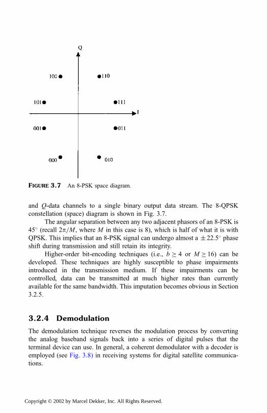
and Q-data channels to a single binary output data stream. The 8-QPSK
constellation (space) diagram is shown in Fig. 3.7.
The angular separation between any two adjacent phasors of an 8-PSK is
45� (recall 2p=M , where M in this case is 8), which is half of what it is with
QPSK. This implies that an 8-PSK signal can undergo almost a � 22.5� phaseshift during transmission and still retain its integrity.
Higher-order bit-encoding techniques (i.e., b � 4 or M � 16) can be
developed. These techniques are highly susceptible to phase impairments
introduced in the transmission medium. If these impairments can be
controlled, data can be transmitted at much higher rates than currently
available for the same bandwidth. This imputation becomes obvious in Section
3.2.5.
3.2.4 Demodulation
The demodulation technique reverses the modulation process by converting
the analog baseband signals back into a series of digital pulses that the
terminal device can use. In general, a coherent demodulator with a decoder is
employed (see Fig. 3.8) in receiving systems for digital satellite communica-
tions.
FIGURE 3.7 An 8-PSK space diagram.
Copyright © 2002 by Marcel Dekker, Inc. All Rights Reserved.
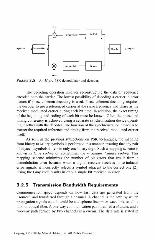
The decoding operation involves reconstructing the data bit sequence
encoded onto the carrier. The lowest possibility of decoding a carrier in error
occurs if phase-coherent decoding is used. Phase-coherent decoding requires
the decoder to use a referenced carrier at the same frequency and phase as the
received modulated carrier during each bit time. In addition, the exact timing
of the beginning and ending of each bit must be known. Often the phase and
timing coherency is achieved using a separate synchronization device operat-
ing together with the decoder. The function of the synchronization device is to
extract the required reference and timing from the received modulated carrier
itself.
As seen in the previous subsections on PSK techniques, the mapping
from binary to M -ary symbols is performed in a manner ensuring that any pair
of adjacent symbols differs in only one binary digit. Such a mapping scheme is
known as Gray coding or, sometimes, the maximum distance coding. This
mapping scheme minimizes the number of bit errors that result from a
demodulation error because when a digital receiver receives noise-induced
error signals, it incorrectly selects a symbol adjacent to the correct one [2].
Using the Gray code results in only a single bit received in error.
3.2.5 Transmission Bandwidth Requirements
Communication speed depends on how fast data are generated from the
‘‘source’’ and transferred through a channel. A channel is the path by which
propagation signals take. It could be a telephone line, microwave link, satellite
link, or optical fiber. A one-way communication path is called a channel, and a
two-way path formed by two channels is a circuit. The data rate is stated in
FIGURE 3.8 An M -ary PSK demodulator and decoder.
Copyright © 2002 by Marcel Dekker, Inc. All Rights Reserved.
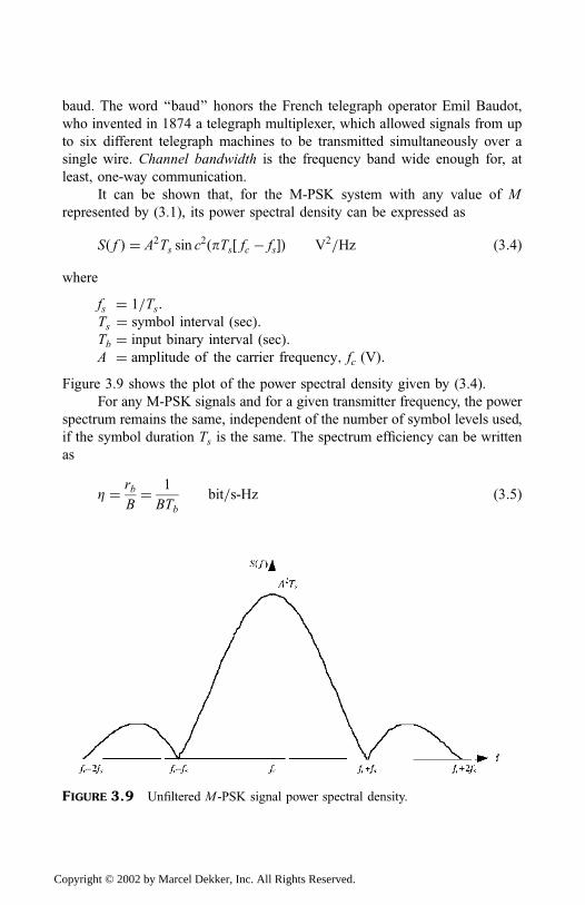
baud. The word ‘‘baud’’ honors the French telegraph operator Emil Baudot,
who invented in 1874 a telegraph multiplexer, which allowed signals from up
to six different telegraph machines to be transmitted simultaneously over a
single wire. Channel bandwidth is the frequency band wide enough for, at
least, one-way communication.
It can be shown that, for the M-PSK system with any value of M
represented by (3.1), its power spectral density can be expressed as
Sð f Þ ¼ A2Ts sin c2ðpTs½ fc � fs�Þ V2=Hz ð3:4Þ
where
fs ¼ 1=Ts:Ts ¼ symbol interval (sec):Tb ¼ input binary interval (sec):A ¼ amplitude of the carrier frequency; fc ðVÞ:
Figure 3.9 shows the plot of the power spectral density given by (3.4).
For any M-PSK signals and for a given transmitter frequency, the power
spectrum remains the same, independent of the number of symbol levels used,
if the symbol duration Ts is the same. The spectrum efficiency can be written
as
Z ¼ rb
B¼ 1
BTbbit=s-Hz ð3:5Þ
FIGURE 3.9 Unfiltered M -PSK signal power spectral density.
Copyright © 2002 by Marcel Dekker, Inc. All Rights Reserved.
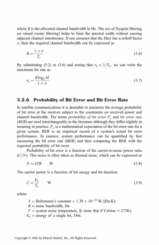
where B is the allocated channel bandwidth in Hz. The use of Nyquist filtering
(or raised cosine filtering) helps to limit the spectral width without causing
adjacent channel interference. If one assumes that the filter has a rolloff factor
a, then the required channel bandwidth can be expressed as
B ¼ 1þ aTs
ð3:6Þ
By substituting (3.2) in (3.6) and noting that rb ¼ 1=Tb; we can write the
maximum bit rate as
rb ¼B log2 M
1þ að3:7Þ
3.2.6 Probability of Bit Error and Bit Error Rate
In satellite communications it is desirable to minimize the average probability
of bit error at the receiver subject to the constraints on received power and
channel bandwidth. The terms probability of bit error Pe and bit error rate
ðBERÞ are used interchangeably in the literature although they differ slightly in
meaning in practice. Pe is a mathematical expectation of the bit error rate for a
given system. BER is an empirical record of a system’s actual bit error
performance. In essence, system performance can be quantified by first
measuring the bit error rate (BER) and then comparing the BER with the
expected probability of bit error.
Probability of bit error is a function of the carrier-to-noise power ratio
(C=N ). This noise is often taken as thermal noise, which can be expressed as
N ¼ kTB W ð3:8Þ
The carrier power is a function of bit energy and bit duration:
C ¼ Eb
TbW ð3:9Þ
where
k ¼ Boltzmann’s constant ¼ 1:38� 10�23 W=ðHz-KÞ:B ¼ noise bandwidth, Hz:T ¼ system noise temperature, K (note that 0�Celsius 273KÞ:Eb ¼ energy of a single bit, J/bit:
Copyright © 2002 by Marcel Dekker, Inc. All Rights Reserved.
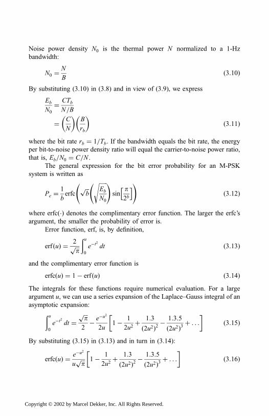
Noise power density N0 is the thermal power N normalized to a 1-Hz
bandwidth:
N0 ¼N
Bð3:10Þ
By substituting (3.10) in (3.8) and in view of (3.9), we express
Eb
N0
¼ CTb
N=B
¼ C
N
� �B
rb
� �ð3:11Þ
where the bit rate rb ¼ 1=Tb. If the bandwidth equals the bit rate, the energy
per bit-to-noise power density ratio will equal the carrier-to-noise power ratio,
that is, Eb=N0 ¼ C=N .
The general expression for the bit error probability for an M-PSK
system is written as
Pe ¼1
berfc
ffiffiffibp
ffiffiffiffiffiffiEb
N0
s !sin
p2b
h i !ð3:12Þ
where erfcð�Þ denotes the complimentary error function. The larger the erfc’s
argument, the smaller the probability of error is.
Error function, erf, is, by definition,
erf ðuÞ ¼ 2ffiffiffipp
ðu0
e�t2
dt ð3:13Þ
and the complimentary error function is
erfcðuÞ ¼ 1� erf ðuÞ ð3:14ÞThe integrals for these functions require numerical evaluation. For a large
argument u, we can use a series expansion of the Laplace–Gauss integral of an
asymptotic expansion:ðu0
e�t2
dt ¼ffiffiffipp2� e�u
2
2u1� 1
2u2þ 1:3
ð2u2Þ2 �1:3:5
ð2u2Þ3 þ . . .
� �ð3:15Þ
By substituting (3.15) in (3.13) and in turn in (3.14):
erfcðuÞ ¼ e�u2
uffiffiffipp 1� 1
2u2þ 1:3
ð2u2Þ2 �1:3:5
ð2u2Þ3 þ . . .
� �ð3:16Þ
Copyright © 2002 by Marcel Dekker, Inc. All Rights Reserved.
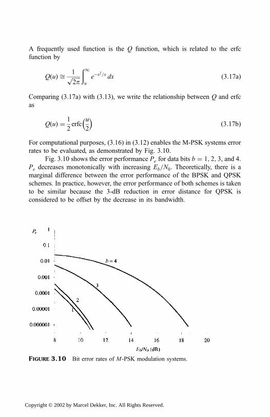
A frequently used function is the Q function, which is related to the erfc
function by
QðuÞ ffi 1ffiffiffiffiffiffi2pp
ð1u
e�x2=x dx ð3:17aÞ
Comparing (3.17a) with (3.13), we write the relationship between Q and erfc
as
QðuÞ ¼ 1
2erfc
u
2
� �ð3:17bÞ
For computational purposes, (3.16) in (3.12) enables the M-PSK systems error
rates to be evaluated, as demonstrated by Fig. 3.10.
Fig. 3.10 shows the error performance Pe for data bits b ¼ 1; 2; 3, and 4.Pe decreases monotonically with increasing Eb=N0. Theoretically, there is a
marginal difference between the error performance of the BPSK and QPSK
schemes. In practice, however, the error performance of both schemes is taken
to be similar because the 3-dB reduction in error distance for QPSK is
considered to be offset by the decrease in its bandwidth.
FIGURE 3.10 Bit error rates of M -PSK modulation systems.
Copyright © 2002 by Marcel Dekker, Inc. All Rights Reserved.
We observe in (3.11) that Eb=N0 is related to carrier power C, input data
bit rate rb, and channel bandwidth B. If Eb=N0 in (3.12) is replaced with the
right-hand terms of (3.11) and the bit rate rb is kept constant, we must increase
the carrier power C to maintain or minimize Pe. This means an increase in the
total power capability of the satellite itself and=or the transmitted power of the
earth station. This might not be possible in many satellite systems that are
power-limited and bandwidth-limited. Increasing power and=or bandwidth is
not a solution to minimizing or reducing the probability of error Pe. An
effective method of reducing Pe in satellite communications is the use of error
correction coding, which is discussed in Chap. 6.
In practice, error performance objectives are usually a compromise
between the performance the user wants and the price he or she is prepared to
pay. Early error performance objectives set by CCIR for an international
telephony channel between two earth stations were that BER should be better
than
1 in 106 (i.e., 10-min mean value) for at least 80% of any month
1 in 104 (i.e., 1-min mean value) for at least 99.7% of any month
1 in 103 (i.e., 1-sec mean value) for at least 99.99% of any year
For connection via the satellite system, the BER should exceed 1 in 103 (i.e.,
1-sec mean value) more than 99.97% of the time. A typical objective for
business systems (e.g., EUTELSAT SMS Systems) is that BER should exceed
1 in 1010 at least 99% of the year; it is usually necessary to provide error
correction in order to achieve this objective [3]. Other objectives for satellite
links between network points are available with ITU.
3.2.7 Theoretical Limit on Eb=N0 for anErrorfree Performance
Shannon [4] demonstrated that error introduced by an ideal additive white
Gaussian noise (AWGN) in a transmission channel of finite bandwidth B can
be reduced. Doing so is possible—without sacrificing the rate of information
transmission—by encoding information whose transmission bit rate rb does
not exceed the channel capacity, Cc. The AWGN is assumed to have a spectral
density N0=2. Shannon (1948) gave the channel capacity as
Cc ¼ B log2 1þ C
N
� �ð3:18Þ
Copyright © 2002 by Marcel Dekker, Inc. All Rights Reserved.

In view of (3.11), Eq. (3.18) can be written as
Cc ¼ B log2 1þ rbEb
BN0
� �
¼ rbEb
N0
BN0
rbEb
log2 1þ rbEb
BN0
� �� �ð3:19Þ
By taking the limit of Cc as the channel bandwidth tends to infinity (B!1),
we can estimate the theoretical limit the channel places on Eb=N0. By
l’Hopital’s rule [5], the limit of a sequence
limx!1 1þ 1
x
� �x
¼ e ð3:20aÞ
Taking log to base 2 of this expression, we have
limx!1
x log2 1þ 1
x
� �¼ log2 e
¼ 1
loge 2¼ 1:443 ð3:20bÞ
Note that
log2 e ¼log10 e
log10 2¼ 1
loge 2and e ¼ 2:718281828459 . . .
By taking the limit of (3.19) and comparing it with (3.20b), we can write
limB!1
Cc ¼ 1:443rbEb
N0
� �ð3:21Þ
Since rb must always be less than limB!1 Cc, we can write
rb 1:443rbEb
N0
� �ð3:22Þ
Alternatively,
Eb
N0
� 1
1:443� 0:693 ð� �1:6 dBÞ ð3:23Þ
This is the required minimum value of Eb=N0, the absolute limit the channel
capacity places to communicate with an errorfree performance. In other words,
a coding scheme exists that allows an arbitrarily low error rate. For example,
PSK modulation requires Eb=N0 9:6 dB to achieve Pe ¼ 10�5. Relating this
Copyright © 2002 by Marcel Dekker, Inc. All Rights Reserved.
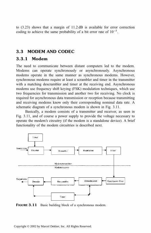
to (3.23) shows that a margin of 11.2 dB is available for error correction
coding to achieve the same probability of a bit error rate of 10�5.
3.3 MODEM AND CODEC
3.3.1 Modem
The need to communicate between distant computers led to the modem.
Modems can operate synchronously or asynchronously. Asynchronous
modems operate in the same manner as synchronous modems. However,
synchronous modems require at least a scrambler and timer in the transmitter
with a matching descrambler and timer at the receiving end. Asynchronous
modems use frequency shift keying (FSK) modulation techniques, which use
two frequencies for transmission and another two for receiving. No clock is
required for asynchronous data transmission or reception because transmitting
and receiving modems know only their corresponding nominal data rate. A
schematic diagram of a synchronous modem is shown in Fig. 3.11.
Basically, a modem consists of a transmitter and receiver, as seen in
Fig. 3.11, and of course a power supply to provide the voltage necessary to
operate the modem’s circuitry (if the modem is a standalone device). A brief
functionality of the modem circuitries is described next.
FIGURE 3.11 Basic building block of a synchronous modem.
Copyright © 2002 by Marcel Dekker, Inc. All Rights Reserved.
Encoder and Decoder
An encoder is an option built into many modems. It is used in conjunction
with some modulation schemes, enabling each signal to represent more than
one bit of information. Encoding can be either binary (bit by bit) or group
(groups of bits). The encoding scheme may be augmented by a forward error
correction technique to improve performance.
For a synchronous modem’s received timer to function properly, it must
remain in synchronization with the data being received. This requires enough
changes in the composition of the data—for instance, 0 to 1 and 1 to 0—to
permit the receiving modem’s circuitry to derive timing from the received data.
A clocking signal tells the terminal device when to sample the received data.
To prevent slipping of the data relative to the modems’ clocks, the data are
always grouped in very short blocks (characters) with framing (start and stop)
bits. Since the data stream can consist of an arbitrary bit pattern, it is possible
for data to randomly contain long sequences of 0s and 1s. When these
sequences occur, the data will not provide the modem’s receiver with
enough transitions for clock recovery, a condition that necessitated the
inclusion of scramblers into synchronous modems.
Decoding involves reconstructing the data bit sequence encoded onto
the carrier. As indicated in Sec. 3.2.4, when phase-coherent decoding is used,
the lowest possibility of decoding a carrier in error occurs. As such, phase-
coherent decoding requires the decoder to use a referenced carrier, possibly
from the ‘‘carrier detector’’ at the same frequency and phase as the received
modulated carrier during each bit time. In addition, the exact timing of the
beginning and end of each bit must be known.
Scrambler and Descrambler
Scrambling is a coding operation applied to the input information message at
the transmitter to randomize the input bit stream. Scrambling eliminates long
strings of similar bits that might impair receiver synchronization and periodic
bit patterns, which could produce undesirable discrete-frequency components
in the power spectrum. In essence, a scrambler modifies the data to be
modulated based on a predefined algorithm. A matching descrambler is
required at the receiving end so that, after demodulation, the randomized
sequence is stripped off. The operation of scrambler and descrambler is
discussed with the aid of Fig. 3.12.
The scrambler takes the form of a shift register with feedback connec-
tions, while the descrambler is a feedforward connected shift register. A
primary reason for the choice of Fig. 3.12 is bit error propagation. A single bit
Copyright © 2002 by Marcel Dekker, Inc. All Rights Reserved.
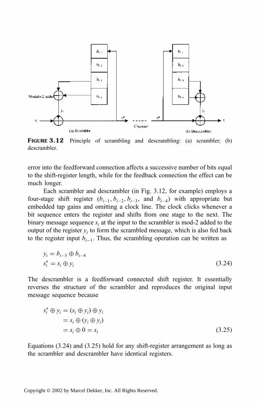
error into the feedforward connection affects a successive number of bits equal
to the shift-register length, while for the feedback connection the effect can be
much longer.
Each scrambler and descrambler (in Fig. 3.12, for example) employs a
four-stage shift register (bi�1; bi�2; bi�3, and bi�4) with appropriate but
embedded tap gains and omitting a clock line. The clock clicks whenever a
bit sequence enters the register and shifts from one stage to the next. The
binary message sequence si at the input to the scrambler is mod-2 added to the
output of the register yi to form the scrambled message, which is also fed back
to the register input bi�1. Thus, the scrambling operation can be written as
yi ¼ bi�3 � bi�4s�i ¼ si � yi ð3:24Þ
The descrambler is a feedforward connected shift register. It essentially
reverses the structure of the scrambler and reproduces the original input
message sequence because
s�i � yi ¼ ðsi � yiÞ � yi
¼ si � ðyi � yiÞ¼ si � 0 ¼ si ð3:25Þ
Equations (3.24) and (3.25) hold for any shift-register arrangement as long as
the scrambler and descrambler have identical registers.
FIGURE 3.12 Principle of scrambling and descrambling: (a) scrambler; (b)
descrambler.
Copyright © 2002 by Marcel Dekker, Inc. All Rights Reserved.
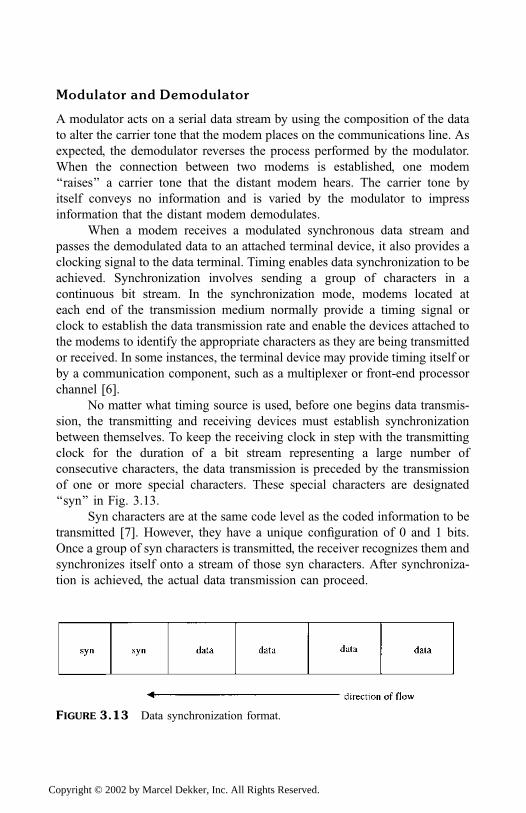
Modulator and Demodulator
A modulator acts on a serial data stream by using the composition of the data
to alter the carrier tone that the modem places on the communications line. As
expected, the demodulator reverses the process performed by the modulator.
When the connection between two modems is established, one modem
‘‘raises’’ a carrier tone that the distant modem hears. The carrier tone by
itself conveys no information and is varied by the modulator to impress
information that the distant modem demodulates.
When a modem receives a modulated synchronous data stream and
passes the demodulated data to an attached terminal device, it also provides a
clocking signal to the data terminal. Timing enables data synchronization to be
achieved. Synchronization involves sending a group of characters in a
continuous bit stream. In the synchronization mode, modems located at
each end of the transmission medium normally provide a timing signal or
clock to establish the data transmission rate and enable the devices attached to
the modems to identify the appropriate characters as they are being transmitted
or received. In some instances, the terminal device may provide timing itself or
by a communication component, such as a multiplexer or front-end processor
channel [6].
No matter what timing source is used, before one begins data transmis-
sion, the transmitting and receiving devices must establish synchronization
between themselves. To keep the receiving clock in step with the transmitting
clock for the duration of a bit stream representing a large number of
consecutive characters, the data transmission is preceded by the transmission
of one or more special characters. These special characters are designated
‘‘syn’’ in Fig. 3.13.
Syn characters are at the same code level as the coded information to be
transmitted [7]. However, they have a unique configuration of 0 and 1 bits.
Once a group of syn characters is transmitted, the receiver recognizes them and
synchronizes itself onto a stream of those syn characters. After synchroniza-
tion is achieved, the actual data transmission can proceed.
FIGURE 3.13 Data synchronization format.
Copyright © 2002 by Marcel Dekker, Inc. All Rights Reserved.
Equalization Filter
An equalization filter (also called simply an equalizer) is used to remove a
large part of the intersymbol interference introduced by channel filtering [8]. A
channel filter, as in Fig. 3.11, is used to remove the channel’s extraneous tones
caused by noise that may have escaped filtering prior to transmission.
To illustrate the basic idea of an equalizer, consider a channel perturbing
the received signal, say yðtÞ, with white Gaussian noise with double-sided
power spectral density ð1=2ÞN0. Let’s formulate the received signal as
yðtÞ ¼ sdðtÞ þ bcsdðt � tDÞ þ nðtÞ ð3:26Þ
where
bc ¼ Attenuation due to intersymbol interference.
ti ¼ Delay induced by intersymbol interference.
sdðtÞ ¼ AdðtÞ cos oct:dðtÞ ¼Data stream: a sequence of �1, each of which is T sec in
duration.
A ¼ voltage level.
If we take the Fourier transform of this expression and—although important—
the noise component nðtÞ is neglected for simplicity, the transfer function of
the channel is
Hcð f Þ ¼=½ yðtÞ�=½sdðtÞ�
¼ 1þ bce�j2ptDf ð3:27Þ
If bc and tD are known, the equalizer will have a transfer function of
Heqð f Þ ¼1
Hcð f Þð3:28Þ
This expression leads to the concept of an inverse filter: a filter best matched to
the incoming signal to achieve optimal reception. This type of filter is called a
matched filter. Since bc and tD will not be exact or may even change with time,
we must allow for adjusting the parameters of the equalizer. If we restrict
ourselves to transversal or tapped delay-line structures for the purpose of
equalization, we can develop a simple algorithm for estimating the tap weights
an using either a zero forcing or minimum mean-square error technique. These
techniques are described in the next subsections.
Copyright © 2002 by Marcel Dekker, Inc. All Rights Reserved.
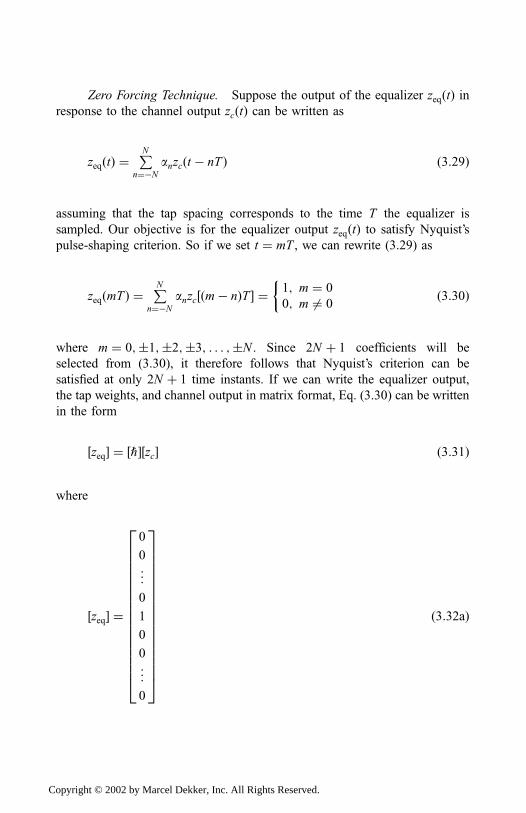
Zero Forcing Technique. Suppose the output of the equalizer zeqðtÞ inresponse to the channel output zcðtÞ can be written as
zeqðtÞ ¼PN
n¼�Nanzcðt � nT Þ ð3:29Þ
assuming that the tap spacing corresponds to the time T the equalizer is
sampled. Our objective is for the equalizer output zeqðtÞ to satisfy Nyquist’s
pulse-shaping criterion. So if we set t ¼ mT , we can rewrite (3.29) as
zeqðmT Þ ¼PN
n¼�Nanzc½ðm� nÞT � ¼ 1; m ¼ 0
0; m 6¼ 0
ð3:30Þ
where m ¼ 0;�1;�2;�3; . . . ;�N . Since 2N þ 1 coefficients will be
selected from (3.30), it therefore follows that Nyquist’s criterion can be
satisfied at only 2N þ 1 time instants. If we can write the equalizer output,
the tap weights, and channel output in matrix format, Eq. (3.30) can be written
in the form
½zeq� ¼ ½h�½zc� ð3:31Þ
where
½zeq� ¼
0
0
..
.
0
1
0
0
..
.
0
266666666666666664
377777777777777775
ð3:32aÞ
Copyright © 2002 by Marcel Dekker, Inc. All Rights Reserved.
that is, N zeros at the top and bottom of 1;
½h� ¼
a�Na�Nþ1a�Nþ2
..
.
a0a1...
aN
26666666666664
37777777777775
ð3:32bÞ
and
zc� � ¼
zcð0Þ zcð�T Þ . . . zcð�2NT ÞzcðT Þ zcð0Þ . . . zc½ð�2N þ 1ÞT �... ..
.. . . ..
.
zcð2NT Þ zc½ð2N � 1ÞT � . . . zcð0Þ
26664
37775 ð3:32cÞ
The preceding procedure describes the zero forcing technique. Since ½zeq� isspecified by the zero forcing condition, all that is required is to find ½zc��1; thatis, the inverse of ½zc�. The desired coefficient matrix ½h� is then the middle
column of ½zc��1, which follows by multiplying ½zc��1 and ½zeq�.As a refresher, the inverse of a nonsingular matrix A is defined as
A�1 ¼ Aadj
jAj
where Aadj denotes the adjoint matrix of A, and jAj denotes the determinant of
A. For example, if A is a square matrix, its adjoint is the transpose of the
matrix obtained from A by replacing each element of A by its cofactor. This
definition becomes clearer with an illustration.
Example 3.1: Find the inverse of matrix A defined by
A ¼1 2 0
3 �1 �21 0 �3
24
35 ð3:33aÞ
Copyright © 2002 by Marcel Dekker, Inc. All Rights Reserved.
The adjoint of matrix A is obtained as
Aadj ¼
�1 �20 �3
�������� � 2 0
0 �3
�������� 2 0
�1 �2
��������
� 3 �21 �3
�������� 1 0
1 �3
�������� � 1 0
3 �2
��������
3 �11 0
�������� � 1 2
1 0
�������� 1 2
3 �1
��������
2666666664
3777777775
¼3 6 �47 �3 2
1 2 �7
264
375 ð3:33bÞ
noting that the determinant of
C ¼a b c
d e f
g h i
264
375
¼ a½ei� fh� � b½di� gf � þ c½dh� eg� ð3:33cÞIn view of (3.33c), the determinant of A is
jAj ¼ 17 ð3:33dÞHence, the inverse matrix is
A�1 ¼ Aadj
jAj ¼3=17 6=17 �4=177=17 �3=17 2=17
1=17 2=17 �7=17
264
375 ð3:33eÞ
As an exercise for the reader, show that AAadj is a diagonal matrix with
diagonal elements equal to jAj; that is,AAadj ¼ AadjA ¼ jAjI
¼ jAj1 0 0
0 1 0
0 0 1
264
375 ð3:33f Þ
To have a feel for the algorithm described by (3.31), we use Example 3.2 as an
illustration.
Copyright © 2002 by Marcel Dekker, Inc. All Rights Reserved.
Example 3.2: Consider a transmission channel for which the following
sample values of its pulse response are given as
zcð0Þ ¼ 1:0 zcðT Þ ¼ 0:3 zcð2T Þ ¼ �0:07zcð�2T Þ ¼ �0:05zcð�T Þ ¼ 0:2
Solution
We can therefore write the channel output matrix as
½zc� ¼1:0 0:2 �0:050:3 1:0 0:2�0:07 0:3 1:0
24
35 ð3:34aÞ
and its inverse matrix becomes
½zc��1 ¼1:0815 �0:2474 0:1035�0:3613 1:1465 �0:24740:1841 �0:3613 1:0815
24
35 ð3:34bÞ
The desired coefficient ½h� is½h� ¼ ½zc��1½zeq�
¼1:0815 �0:2474 0:1035
�0:3613 1:1465 �0:24740:1841 �0:3613 1:0815
264
375 0
1
0
264
375
¼�0:24741:1465
�0:3613
264
375 ð3:34cÞ
This result is, in effect, the middle column of the inverse matrix that gives the
zero forcing tap coefficients. Using these desired coefficients, the equalizer
output is thus expressed as
zeqðmT Þ ¼ �0:2474zc½ðmþ 1ÞT � þ 1:1465zcðmT Þ � 0:3613zc½ðm� 1ÞT �ð3:34dÞ
The equalizer response of zeqðmT Þ;m ¼ �1; 0; 1 at constant sample time
T ¼ 1, is shown in Fig. 3.14.
Minimum Mean-Square Error (MMSE) Technique. The concept of the
MMSE is to seek the tap weights that minimize the mean-square error between
the desired output from the equalizer and the actual output at any given time t.
Copyright © 2002 by Marcel Dekker, Inc. All Rights Reserved.
We denote the desired and actual equalizer’s output by zdðtÞ and zaðtÞrespectively. So the MMSE technique is expressed as [3]
e ¼ Ef½zaðtÞ � zdðtÞ�2g ð3:35Þwhere Ef�g denotes the expectation of f�g. Like (3.29), the actual output is
zaðtÞ ¼PN
n¼�Nanzcðt � nDÞ ð3:36Þ
where, in this instance, the tap spacing D does not correspond to the sampling
time. Our task is to set a sufficient condition to minimize the tap weights an.Since e is a concave function of an, then a sufficient condition for error
minimization is
@e@an¼ 0 ¼ 2E ½zaðtÞ � zdðtÞ�
@zaðtÞ@an
; n ¼ 0; �1; . . . ;�N ð3:37Þ
Upon substituting (3.36) in (3.37) and differentiating the resultant, we obtain
the conditions
Ef½zaðtÞ � zdðtÞ�zcðt � nDÞg ¼ 0; n ¼ 0;�1; . . . ;�N ð3:38ÞAlternatively,
Ef½zdðtÞ�zcðt � nDÞg ¼ Ef½zaðtÞ�zcðt � nDÞg ð3:39ÞLet’s pause to emphasize what we have obtained in terms of data autocorrela-
tion. By definition, cross correlation of signals x and y is
RxyðtÞ ¼ EfxðtÞyðt þ tÞg ð3:40aÞ
FIGURE 3.14 The three-tap equalizer response using zero forcing technique.
Copyright © 2002 by Marcel Dekker, Inc. All Rights Reserved.
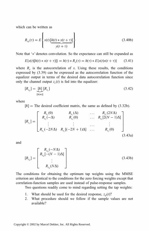
which can be written as
RxyðtÞ ¼ E xðtÞ ½hðtÞ � xðt þ tÞ�|fflfflfflfflfflfflfflfflfflfflffl{zfflfflfflfflfflfflfflfflfflfflffl}yðt þ tÞ
8><>:
9>=>; ð3:40bÞ
Note that ‘�’ denotes convolution. So the expectance can still be expanded as
EfxðtÞ½hðtÞ � xðt þ tÞ�g ¼ hðtÞ � RxðtÞ ¼ hðtÞ � EfxðtÞxðt þ tÞg ð3:41Þwhere Rx is the autocorrelation of x. Using these results, the conditions
expressed by (3.39) can be expressed as the autocorrelation function of the
equalizer output in terms of the desired data autocorrelation function since
only the channel output zcðtÞ is fed into the equalizer:
½Rzd� ¼ ½h�|{z}
½hðmÞ�½Rzc� ð3:42Þ
where
½h� ¼ The desired coefficient matrix, the same as defined by (3.32b).
½Rzc� ¼
Rzcð0Þ Rzc
ðDÞ . . . Rzcð2NDÞ
Rzcð�DÞ Rzc
ð0Þ . . . Rzc½2ðN � 1ÞD�
..
. ...
. . . ...
Rzcð�2NDÞ Rzc
½ð�2N þ 1ÞD� . . . Rzcð0Þ
26664
37775ð3:43aÞ
and
½Rzd� ¼
Rzdð�NDÞ
Rzd�ðN � 1ÞD½ �
..
.
RzdðNDÞ
26664
37775 ð3:43bÞ
The conditions for obtaining the optimum tap weights using the MMSE
criterion are identical to the conditions for the zero forcing weights except that
correlation-function samples are used instead of pulse-response samples.
Two questions readily come to mind regarding setting the tap weights:
1. What should be used for the desired response, zdðtÞ?2. What procedure should we follow if the sample values are not
available?
Copyright © 2002 by Marcel Dekker, Inc. All Rights Reserved.
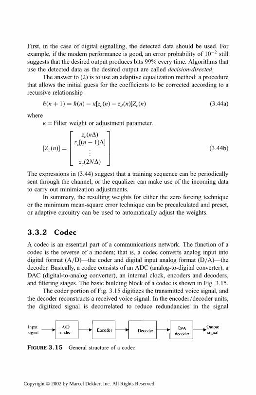
First, in the case of digital signalling, the detected data should be used. For
example, if the modem performance is good, an error probability of 10�2 stillsuggests that the desired output produces bits 99% every time. Algorithms that
use the detected data as the desired output are called decision-directed.
The answer to (2) is to use an adaptive equalization method: a procedure
that allows the initial guess for the coefficients to be corrected according to a
recursive relationship
hðnþ 1Þ ¼ hðnÞ � k½zcðnÞ � zdðnÞ�ZcðnÞ ð3:44aÞwhere
k¼ Filter weight or adjustment parameter.
½ZcðnÞ� ¼zcðnDÞ
zc½ðn� 1ÞD�...
zcð2NDÞ
26664
37775 ð3:44bÞ
The expressions in (3.44) suggest that a training sequence can be periodically
sent through the channel, or the equalizer can make use of the incoming data
to carry out minimization adjustments.
In summary, the resulting weights for either the zero forcing technique
or the minimum mean-square error technique can be precalculated and preset,
or adaptive circuitry can be used to automatically adjust the weights.
3.3.2 Codec
A codec is an essential part of a communications network. The function of a
codec is the reverse of a modem; that is, a codec converts analog input into
digital format (A=D)—the coder and digital input analog format (D=A)—the
decoder. Basically, a codec consists of an ADC (analog-to-digital converter), a
DAC (digital-to-analog converter), an internal clock, encoders and decoders,
and filtering stages. The basic building block of a codec is shown in Fig. 3.15.
The coder portion of Fig. 3.15 digitizes the transmitted voice signal, and
the decoder reconstructs a received voice signal. In the encoder=decoder units,the digitized signal is decorrelated to reduce redundancies in the signal
FIGURE 3.15 General structure of a codec.
Copyright © 2002 by Marcel Dekker, Inc. All Rights Reserved.
because a voice signal is usually highly correlated. The filtering stages form
part of internal constructs of encoder=decoder units. Their function is to
suppress low-frequency noise and apply an anti-aliasing process to it.
Various types of codecs are available, and their applications vary as the
network demands. However, the levels of programmability, the clock frequen-
cies, and the fabrication technologies used dictate the difference. The codec
also coordinates the timing between itself and the network(s) with which it
interfaces. Data transmission is synchronized and multiplexed. To maintain the
industry standard of voice signal quality, the digitized voice signal must have a
signal-to-distortion level of at least 30 dB over a 40-dB dynamic range [9]. In
order to meet this specification, two methods of data reduction (companding)
have been specified: m-law (also called Mu-255 law) and A-law.
Companding, simply a compression and expansion process, is used to
upgrade the quality of the pulse, which increases the signal-to-noise ratio and
reduces peak power to prevent overloading. Both the encoder and decoder
units of the codec perform companding.
The m-law companding technique is the standard used in North America
and Japan, whereas the A-law companding technique is the accepted standard
in Europe. Most codec manufacturers have developed a device that meets both
companding techniques. These laws are logarithmics:
m-law:
Y ¼ lnð1þ mjxjÞlnð1þ mÞ ð3:45Þ
where
Y ¼Coding range.
x¼Amplitude, �1 x 1.
The value of m is determined by the law and is constant.
A-law:
Y ¼ 1þ lnðAjxjÞ1þ lnðAÞ ; where
1
A jxj 1 ð3:46Þ
Y ¼ Ax
1þ lnðAÞ ; where 0 jxj 1
Að3:47Þ
The value of A is determined by the law and is constant.
The main difference between m-law and A-law is that in A-law the
normalized amplitude x is replaced with a signal whose amplitude is smaller
Copyright © 2002 by Marcel Dekker, Inc. All Rights Reserved.
than 1=A. Whichever law is used, the prime objective of companding rules is
to guarantee a quantization ratio proportional to the size of the original signal.
The most important noise affecting codec design is the idle channel
noise, which exists even when there is no signal traffic. This idle channel noise
occurs due to the quantization of a 0-V input analog signal as the digital output
bounces around the assigned binary value for zero along with any nonlinearity
existing along the transmission line.
3.3.3 Summary
Modems can be segmented according to their usage by the modulation
schemes utilized:
Frequency division multiplexing (FDM) for traffic and video
Single channel per carrier (SCPC) for voice channels’ low-level carrier
Time division multiplexing=time division multiple access (TDM=TDMA) for data transmission over satellite links and to data users
Spread spectrum modems, particularly by military satellite communica-
tions
The configuration and modulation=demodulation scheme deployed and their
performance characteristics separate one modem from another. Intersymbol
interference introduced by channel filtering can be removed to a large part by
zero forcing and mimimum mean-square error techniques. Carrier acquisition
and symbol synchronization or timing extraction are critical to the operation of
high-performance modems. With the gradual change to digital transmission,
codecs, will become a common feature.
3.4 EARTH STATION DESIGN CONSIDERATIONS
Earth stations form an important part of the overall satellite system. In general,
when designing an earth station, the following must be considered, including
implementation restrictions:
1. System parameters such as
Transmitter EIRP.
Receiver figure of merit (G=T)—quality of received signal.
System noise and other interference including site location, en-
suring that the total interference level does not exceed the
acceptable level. Interference to, from, and between satellite
Copyright © 2002 by Marcel Dekker, Inc. All Rights Reserved.
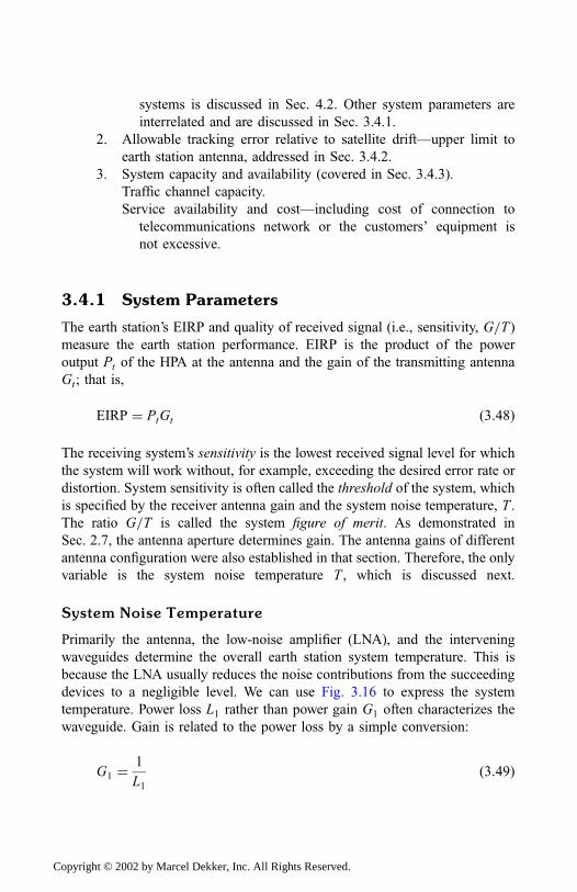
systems is discussed in Sec. 4.2. Other system parameters are
interrelated and are discussed in Sec. 3.4.1.
2. Allowable tracking error relative to satellite drift—upper limit to
earth station antenna, addressed in Sec. 3.4.2.
3. System capacity and availability (covered in Sec. 3.4.3).
Traffic channel capacity.
Service availability and cost—including cost of connection to
telecommunications network or the customers’ equipment is
not excessive.
3.4.1 System Parameters
The earth station’s EIRP and quality of received signal (i.e., sensitivity, G=T )measure the earth station performance. EIRP is the product of the power
output Pt of the HPA at the antenna and the gain of the transmitting antenna
Gt; that is,
EIRP ¼ PtGt ð3:48Þ
The receiving system’s sensitivity is the lowest received signal level for which
the system will work without, for example, exceeding the desired error rate or
distortion. System sensitivity is often called the threshold of the system, which
is specified by the receiver antenna gain and the system noise temperature, T .
The ratio G=T is called the system figure of merit. As demonstrated in
Sec. 2.7, the antenna aperture determines gain. The antenna gains of different
antenna configuration were also established in that section. Therefore, the only
variable is the system noise temperature T , which is discussed next.
System Noise Temperature
Primarily the antenna, the low-noise amplifier (LNA), and the intervening
waveguides determine the overall earth station system temperature. This is
because the LNA usually reduces the noise contributions from the succeeding
devices to a negligible level. We can use Fig. 3.16 to express the system
temperature. Power loss L1 rather than power gain G1 often characterizes the
waveguide. Gain is related to the power loss by a simple conversion:
G1 ¼1
L1ð3:49Þ
Copyright © 2002 by Marcel Dekker, Inc. All Rights Reserved.
In view of (3.8), the noise power at the output of the waveguide can be written
as
N ¼ kB
L1ðTa þ Te1Þ ð3:50Þ
where Ta and Te1 respectively correspond to the antenna noise temperature and
waveguide noise temperature. The equivalent noise temperature Tex for a lossy
two-port system whose power loss L is greater than unity can be related to the
absolute temperature T0; using the expression
Tex ¼ T0ðL� 1Þ ð3:51Þ
Hence, we can write the waveguide noise temperature as
Te1 ¼ T0ðL1 � 1Þ ð3:52Þ
Substituting (3.52) in (3.50), we have the noise power at the output of the
waveguide
N ¼ kBTa
L1þ T0ðL1 � 1Þ
L1
� �ð3:53Þ
By comparing (3.53) with (3.8), the equivalent noise temperature at the
waveguide’s output is
Tw ¼Ta
L1þ T0ðL1 � 1Þ
L1ð3:54Þ
The earth station system noise temperature referred to the input of the LNA
simply is
T ¼ Tw þ Te ð3:55Þ
FIGURE 3.16 Block diagram for estimating system noise temperature.
Copyright © 2002 by Marcel Dekker, Inc. All Rights Reserved.
where Te is the equivalent temperature, considering the contributions from
LNA and other devices, as seen at the LNA input (at the dotted line point of
Fig. 3.15):
Te ¼ Te2 þTe3
G2
ð3:56Þ
By substituting (3.56) and (3.54) in (3.55), we see that the system noise
temperature is
T ¼ Ta
L1þ T0ðL1 � 1Þ
L1þ Te2 þ
Te3
G2
ð3:57Þ
With the gain expressions developed for different kinds of antennas in Sec. 2.7
and the system noise temperature in (3.57), we can establish the earth station
sensitivity G=T.
Example 3.3: A 20-m Cassegrain antenna, having a receive antenna gain of
54.53 dB at 11.2GHz and an ambient temperature of 275K, is characterized
by the following parameters:
Antenna noise temperature¼ 60K.
Waveguide loss¼ 0.3 dB.
Low-noise amplifier (LNA) with 20-dB gain and 350K effective noise
temperature.
Effective noise temperature of the downconverter¼ 1500K.
Estimate (1) the earth station system noise temperature and (2) the antenna
gain referred to the input of the LNA.
Solution
L1 ¼ 100:03 ¼ 1:0715 G2 ¼ 20 dB ¼ 102 ¼ 100
Ta ¼ 60 T0 ¼ 275 Te3 ¼ 1500 Te2 ¼ 350
1. Using (3.57), we can calculate the earth station temperature as
T ¼ 60
1:0715þ 275 � 0:0715
1:0715þ 350þ 1500
100¼ 439:345 K
2. Antenna gain referred to the input of LNA: Ga ¼ ð54:53� 0:3Þ ¼54:50 dB.
Copyright © 2002 by Marcel Dekker, Inc. All Rights Reserved.
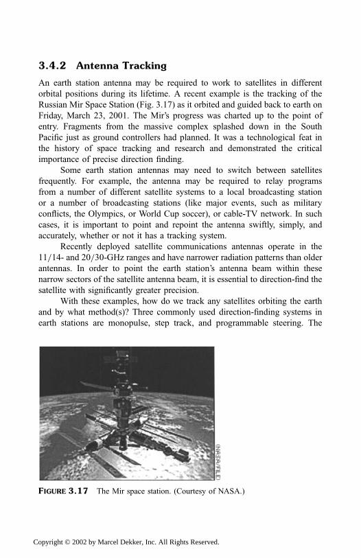
3.4.2 Antenna Tracking
An earth station antenna may be required to work to satellites in different
orbital positions during its lifetime. A recent example is the tracking of the
Russian Mir Space Station (Fig. 3.17) as it orbited and guided back to earth on
Friday, March 23, 2001. The Mir’s progress was charted up to the point of
entry. Fragments from the massive complex splashed down in the South
Pacific just as ground controllers had planned. It was a technological feat in
the history of space tracking and research and demonstrated the critical
importance of precise direction finding.
Some earth station antennas may need to switch between satellites
frequently. For example, the antenna may be required to relay programs
from a number of different satellite systems to a local broadcasting station
or a number of broadcasting stations (like major events, such as military
conflicts, the Olympics, or World Cup soccer), or cable-TV network. In such
cases, it is important to point and repoint the antenna swiftly, simply, and
accurately, whether or not it has a tracking system.
Recently deployed satellite communications antennas operate in the
11=14- and 20=30-GHz ranges and have narrower radiation patterns than older
antennas. In order to point the earth station’s antenna beam within these
narrow sectors of the satellite antenna beam, it is essential to direction-find the
satellite with significantly greater precision.
With these examples, how do we track any satellites orbiting the earth
and by what method(s)? Three commonly used direction-finding systems in
earth stations are monopulse, step track, and programmable steering. The
FIGURE 3.17 The Mir space station. (Courtesy of NASA.)
Copyright © 2002 by Marcel Dekker, Inc. All Rights Reserved.
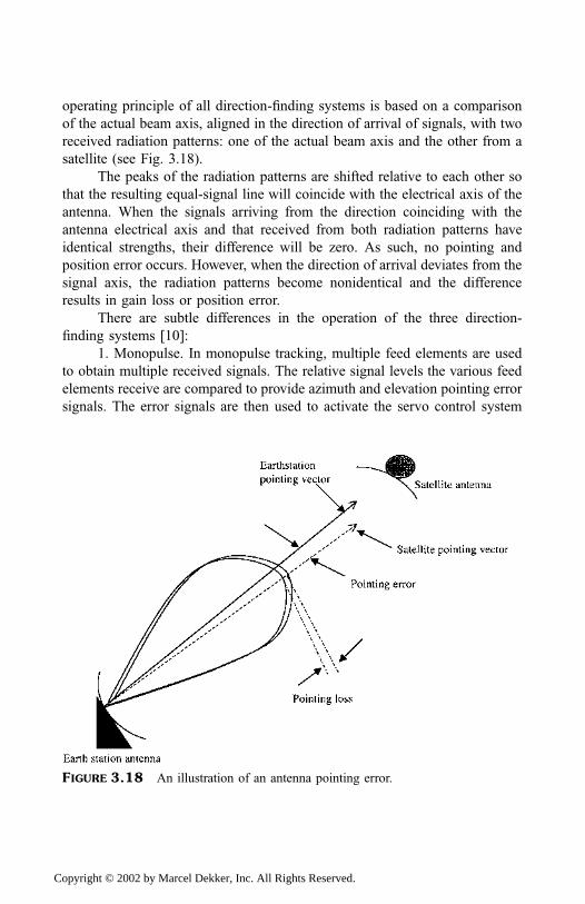
operating principle of all direction-finding systems is based on a comparison
of the actual beam axis, aligned in the direction of arrival of signals, with two
received radiation patterns: one of the actual beam axis and the other from a
satellite (see Fig. 3.18).
The peaks of the radiation patterns are shifted relative to each other so
that the resulting equal-signal line will coincide with the electrical axis of the
antenna. When the signals arriving from the direction coinciding with the
antenna electrical axis and that received from both radiation patterns have
identical strengths, their difference will be zero. As such, no pointing and
position error occurs. However, when the direction of arrival deviates from the
signal axis, the radiation patterns become nonidentical and the difference
results in gain loss or position error.
There are subtle differences in the operation of the three direction-
finding systems [10]:
1. Monopulse. In monopulse tracking, multiple feed elements are used
to obtain multiple received signals. The relative signal levels the various feed
elements receive are compared to provide azimuth and elevation pointing error
signals. The error signals are then used to activate the servo control system
FIGURE 3.18 An illustration of an antenna pointing error.
Copyright © 2002 by Marcel Dekker, Inc. All Rights Reserved.
controlling antenna pointing. The monopulse method is used in systems that
utilize polarization isolation, when greater satellite tracking precision is
necessary—for example, in INTELSAT antennas.
2. Step track method. In the step track method, the radiation pattern of
the antenna is shifted discretely in small ‘‘steps.’’ The position corresponding
to the peak signal is determined by measuring the sign of the difference of the
signal levels before and after a step. The differential yields the step size for the
next change in position alternately in azimuth and elevation. The iteration
process is interrupted when the position is optimum, that is, when the
differential is negligibly small. The advantages of the step track method are
its simplicity and relative low cost. Its disadvantage is its low speed.
3. Programmable steering method. In this technique, antenna pointing is
based upon knowledge of the relative motion of the satellite with respect to the
earth station. A mathematical function, together with the known geographical
coordinates of the earth station, is programmed and used to update the antenna
pointing without reference to a signal received from the satellite. This
technique is independent of earth station’s performance and link parameters,
yet it is relatively complex to achieve considerable precision accuracy.
In general, whichever scheme is implemented and in order to prevent the
pointing loss, the main lobe of the earth station’s antenna must be pointed
automatically or manually at the satellite with the greatest possible accuracy.
This operation is performed by the tracking system that, by means of its
various control loops, ensures that the position errors of the antenna main
beam (e.g., due to wind or satellite drift) from the ideal satellite position are
compensated. The antenna tracking system together with the tracking servo
system, the drive electronics, the electric drives, and the antenna form a closed
control loop. The servo system processes the error signals supplied by the
tracking receiver and prepares them for the drive electronics that control the dc
motors on the antenna axis. The electric drive supplies the drive torque
through mechanical gears to the antenna axis and compensates the gears’
backlash by producing bias torque.
3.4.3 System Capacity, Cost, and Availability
Like the satellite system availability analysis performed in Sec. 2.6.5, a similar
analysis must be performed for the earth station’s system availability. Cost is
determined by what the customers want, what level of performance has been
guaranteed, and what is technically achievable. Whether an earth station is
owned or leased, it is important that selected equipment meet the operational
Copyright © 2002 by Marcel Dekker, Inc. All Rights Reserved.
performance of the satellite communications to be networked to and that each
unit of a particular equipment closely match the performance of the other. This
ensures that the overall system is consistently superior with a high reliability
factor, thereby guaranteeing high performance.
System Capacity
Video (TV), voice (telephone), and data signals from users via the public-
switched data networks (e.g., integrated service digital network, or ISDN) are
brought through the terrestrial link (e.g., optical fiber, twisted pair cable,
coaxial cable, microwave link) from different sources to the earth station.
Terrestrial links are investigated in Sec. 3.5. ISDN basically evolved from
telephone networks with an emphasis on multiplexing and switching arrange-
ments, offering a variety of services to a large number of users. ISDN is
explored in Chap. 8. Naturally, an earth station may accept traffic from a
number of independent terrestrial carriers. The carriers may have been
assembled in different access formats (e.g., TDMA, FDMA, or CDMA—
more about these access formats appears in Chap. 5). In some applications,
earth stations may operate in a transponding mode with the same or different
assemblies, in which received satellite signals are used to initiate a retrans-
mission from the station to another station or to the satellite. As such, it may
be necessary to extract a few channels from each of a number of large
assemblies and to disassemble them to the channel level. In this case the
amount of demultiplexing necessary at the earth station may be substantial.
The goal of this section is to estimate the channel capacity.
To enhance the reader’s understanding of the subject matter, this section
briefly introduces information theory and then explains channel capacity
analysis. By mastering the basic information theory, the reader will be able
to move on to concrete realizations without great difficulty.
Information Theory. Information theory deals with the mathematical
modelling and analysis of a communication system. It provides limits on
The minimum number of bits per symbol required to fully represent the
information source.
The maximum rate at which reliable communication can take place over
the channel, known as the Shannon bound. The Shannon bound
provides the motivation for coding.
Source Information and Entropy. Figure 3.19 represents a generalized
simple model of a digital communication system. The source data contains M
Copyright © 2002 by Marcel Dekker, Inc. All Rights Reserved.
symbols from a finite source states xi, which are traversed via a discrete
memoryless channel (DMC) to produce data yi.
The output data yi, which contain N symbols, can be viewed as a time
sequence of source states. The term memoryless implies that the source output
is independent of all preceding and succeeding source outputs. For conve-
nience, we write the input and output states as
X ¼ ðx1; x2; x3; . . . ; xM ÞY ¼ ðy1; y2; y3; . . . ; yN Þ
ð3:58Þ
The theory of effective encoding of signals from various sources is a branch of
modern information theory. The results of the theory descend from the
Shannon theorem, which states that the minimum average number of symbols
necessary for data transmission from some sources equals its entropy, H . Thus,
entropy implies the average information associated with the sources; the
average is over all source states. The information I associated with source
states xi is
I ðxiÞ ¼ loga1
pðxiÞð3:59Þ
where a, the base of the logarithm, determines the unit in which the
information is measured. Also, pðxiÞ is the probability that the source state
is transmitted. From elementary mathematics, the sum of the source prob-
abilities is unity:
PMi¼1
pðxiÞ ¼ 1 ð3:60aÞ
Note that
loga k ¼log10 k
log10 að3:60bÞ
Equation (3.59) satisfies these three conditions:
1. I ðxiÞ � 0 within the bound 0 pðxiÞ 1.
2. As pðxiÞ approaches unity, I ðxiÞ approaches zero.
FIGURE 3.19 A generalized model of a digital communication system.
Copyright © 2002 by Marcel Dekker, Inc. All Rights Reserved.
3. For two independent sources, with states xr and xs, the probability of
xr and xs equals the product of their individual state’s probability,
pðxrÞpðxsÞ. Consequently, the information conveyed by the joint
event of the two symbols is
I rs ¼ loga1
pðxrÞpðxsÞ¼ loga
1
pðxrÞþ loga
1
pðxsÞ¼ I r þ I s ð3:61Þ
This expression shows that the information conveyed by the joint event of the
two symbols equals the sum of the information conveyed by each symbol.
Although important, it is not the information associated with source
states but rather the average information associated with the source. Hence, the
entropy of the DMC source can be written as
HðX Þ ¼PMi¼1
pðxiÞ loga1
pðxiÞð3:62Þ
Example 3.4: As an illustration of the meaning of ‘‘entropy,’’ consider a
binary source that generates two symbols 0 and 1, with corresponding
probabilities b and ð1� bÞ. From (3.62), the binary source entropy is
expressed as
HðbÞ ¼ b log21
bþ ð1� bÞ log2
1
1� bð3:63Þ
Using this expression, we can draw the entropy function as in Fig. 3.20.
Figure 3.20 shows that at the two extremes (i.e., when b ¼ 0 and 1) the
source output is always certain, meaning the entropy is zero; HðbÞ ¼ 0.
However, if the symbols’ probabilities are equally probable—that is, when
b ¼ 0:5—the source output is maximally uncertain and the entropy is
maximum, HðbÞ ¼ 1. This condition demonstrates that the entropy can be
interpreted as a measure of uncertainty.
It is easy to generalize for a DMC with a binary symmetric channel
(BSC) in which all M symbols are equally likely to be transmitted and would
have an entropy
HðX Þ ¼ log2ðM Þ ð3:64Þ
Copyright © 2002 by Marcel Dekker, Inc. All Rights Reserved.
Thus, the entropy could be bounded as
0 HðX Þ log2ðM Þ ð3:65ÞThe information transmission rate can be written as
Rr ¼ rbHðX Þ ð3:66Þwhere rb is the data transmission rate (bit=sec).
Conditional Probabilities. Where information is mutually shared
between the channel’s input and output, the entropy measurement is condi-
tional on the quality of information received either way. The entropy is then
interpreted as a conditional measure of uncertainty. Consider a BSC as an
example of a DMC, as seen in Fig. 3.21.
The DMC is defined by a set of transition probabilities. The probability
of transmitting x1 and receiving y1 is pðx1; y1Þ. By Bayes’ theorem, this
probability can be rewritten as
pðx1; y1Þ ¼ pðy1jx1Þpðx1Þ ð3:67aÞAlternatively,
pðx1; y1Þ ¼ pðx1jy1Þpðy1Þ ð3:67bÞwhere
pðy1jx1Þ ¼ probability of receiving y1 given that x1 was transmitted.
pðx1jy1Þ ¼ probability of transmitting x1 given that y1 was received.
pðx1Þ ¼ probability of transmitting x1.
pðy1Þ ¼ probability of receiving y1.
FIGURE 3.20 Entropy of a binary source.
Copyright © 2002 by Marcel Dekker, Inc. All Rights Reserved.
From (3.67), one can write the probability of receiving 0:
pðy1Þ ¼ pðy1jx1Þpðx1Þ þ pðy1jx2Þpðx2Þ ð3:68aÞConversely, the probability of receiving 1 is written as
pðy2Þ ¼ pðy2jx1Þpðx1Þ þ pðy2jx2Þpðx2Þ ð3:68bÞFollowing the preceding procedure, one can generalize for the source symbols
ðx1; x2; x3; . . . ; xM Þ and the output symbols ðy1; y2; y3; . . . ; yN Þ. Since the
forward transition probability pðyj j xiÞ is easy to determine, the receiving
probabilities can be written as
pðyjÞ ¼ pðyj j x1Þpðx1Þ þ pðyj j x2Þpðx2Þ þ pðyj j x3Þpðx3Þ þ � � �þ pðyj j xM ÞpðxM Þ
¼PMi¼1
pðyj j xiÞpðxiÞ ð3:69Þ
The average mutual information I ðX ; Y Þ is the average information transferred
per symbol across the channel; that is,
I ðX ; Y Þ ¼PMi¼1
PNj¼1
pðxi; yjÞI ðxi; yjÞ ð3:70Þ
Comparing this expression with that of the average self-information given by
(3.62), the average mutual information becomes
I ðX ; Y Þ ¼ HðY Þ � HðY j X Þ ð3:71Þ
FIGURE 3.21 A representation of mutual information system using BSC as an
example of DMC.
Copyright © 2002 by Marcel Dekker, Inc. All Rights Reserved.
where
HðY Þ ¼ output entropy, the average information received per
symbol; given by
HðY Þ ¼PNj¼1
pðyjÞ log21
pðyjÞð3:72Þ
HðY jX Þ ¼ conditional entropy, the average information lost per symbol;
given by
HðY jX Þ ¼PMi¼1
PNj¼1
pðxi; yjÞ log21
pðyj j xiÞð3:73Þ
Recognizing the above, we have
PNj¼1
pðxi; yjÞ ¼ pðxiÞ ð3:74Þ
and
pðxi j yiÞ ¼pðxi; yiÞpðyiÞ
ð3:75Þ
In view of (3.72)–(3.75), the average mutual information of (3.71) may be
written as
I ðX ; Y Þ ¼PNj¼1
pðyjÞ log21
pðyjÞ�PM
i¼1
PNj¼1
pðxi; yjÞ log21
pðyj j xiÞð3:76Þ
By following a similar development, the channel input–output mutual infor-
mation is
I ðX ; Y Þ ¼ HðX Þ � HðX j Y Þ ð3:77Þ
Consequently,
I ðX ; Y Þ ¼PMi¼1
pðxiÞ log21
pðxiÞ�PM
i¼1
PNj¼1
pðxi; yjÞ log21
pðxi j yjÞð3:78Þ
Copyright © 2002 by Marcel Dekker, Inc. All Rights Reserved.
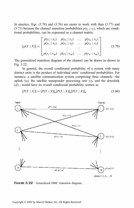
In practice, Eqs. (3.78) and (3.76) are easier to work with than (3.77) and
(3.71) because the channel transition probabilities pðyj j xiÞ, which are condi-
tional probabilities, can be expressed as a channel matrix:
pðY j X Þ½ � ¼pðy1 j x1Þ pðy2 j x1Þ . . . pðyN j x1Þpðy1 j x2Þ pðy2 j x2Þ . . . pðyN j x2Þ
..
. ... ..
. ...
pðy1 j xM Þ pðy2 j xM Þ . . . pðyN j xM Þ
26664
37775 ð3:79Þ
The generalized transition diagram of the channel can be drawn as shown in
Fig. 3.22.
In general, the overall conditional probability of a system with many
distinct units is the product of individual units’ conditional probabilities. For
instance, a satellite communication system comprising three channels—the
uplink ðuÞ, the satellite transponder processing unit ðsÞ, and the downlink
ðdÞ—would have its overall conditional probability written as
PðY j X Þ½ � ¼ PðY j X Þ½ �u PðY j X Þ½ �s PðY j X Þ½ �d ð3:80Þ
FIGURE 3.22 Generalized DMC transition diagram.
Copyright © 2002 by Marcel Dekker, Inc. All Rights Reserved.
To have a feel for this expression, an illustration in the form of Example 3.5
will be examined after the concept of channel capacity has been introduced.
Channel Capacity. Channel capacity is the maximum value of mutual
information I ðY ;X Þ. As an illustration, the BSC as the DMC in Fig. 3.21 is
used to evaluate the channel capacity. The average information transferred is
given by (3.71). The output entropy is
HðY Þ ¼ PN¼2j¼1
pðyjÞ log21
pðyjÞ
¼ pðy1Þ log21
pðy1Þþ pðy2Þ log2
1
pðy2Þð3:81Þ
By allowing the crossover probabilities to be equal ðpðy1 j x2Þ ¼pðy2 j x1Þ ¼ aÞ and the states probabilities to be pðx1Þ ¼ b and pðx2Þ ¼ð1� bÞ, we can write the receiving self-probability using (3.68) as
pðy1Þ ¼ ð1� aÞbþ að1� bÞ ð3:82ÞTherefore, pðy2Þ ¼ 1� pðy1Þ. So, the output entropy becomes
HðY Þ ¼ O pðy1Þð Þ ¼ Oðbþ a� 2abÞ ð3:83ÞFollowing the iterative approach, we can show that the conditional output
entropy is
HðY j X Þ ¼ OðaÞ ð3:84Þwhere Oð Þ is a functional abstract term. This expression depends on the noise
in the channel. Substituting (3.83) and (3.84) in (3.71), the BSC average
mutual information is
I ðX ; Y Þ ¼ Oðbþ a� 2abÞ � OðaÞ ð3:85ÞIn real life a channel is fixed and the channel’s noise is difficult to control. The
objective, therefore, will be to maximize the first Oð Þ-term, the nonnoise
component term, on the right-hand side of (3.85). It was noticed in Fig. 3.20
that the entropy HðbÞ is maximum when the symbols’ source probabilities are
equally probable; that is, b ¼ 0:5. Therefore, we want the nonnoise component
of (3.85) to be
0:5 ¼ ðbþ a� 2abÞ ð3:86Þ
Copyright © 2002 by Marcel Dekker, Inc. All Rights Reserved.

This condition is always satisfied when b ¼ 0:5. This means that if the source
encoder can make b ¼ 0:5 for a BSC, then
1: Channel capacity Cc ¼ 1� OðaÞ bit=symbol ð3:87Þ2: Source information rate Rr ¼ rbOðbÞ bit=sec ð3:88aÞ3: if b ¼ 0:5;Rr ¼ rb bit=sec ð3:88bÞ4: The maximum rate at which information can be transferred across
a BSC channel is
Cm ¼ rbCc ¼ 1� OðaÞ½ �rb bit=sec ð3:89ÞSome books refer to this expression as the channel capacity. In
practice, Eq. (3.87) is often referred to as the channel capacity.
In general, in calculating the channel capacity, whether or not the input data
transfer rate is specified, OðaÞ is replaced with each channel’s self-entropy,
HðX Þ.
Example 3.5: Consider a digital satellite system to comprise three channels:
the uplink, onboard processor, and the downlink. The uplink has an error
probability of 0.001. The processing unit has an error probability of 0.00025.
The downlink error probability is 0.01. Calculate
1. Each channel’s capacity
2. The system’s overall conditional probability
3. The overall system channel capacity
Solution
1. Define each channel’s error probability pðy1Þ. pðy2Þ ¼ 1� pðy1Þ.Using (3.80) and (3.87), we can define each channel capacity as
Cc ¼ 1� pðy1Þ log21
pðy1Þþ pðy2Þ log2
1
pðy2Þ� �
bit=symbol
ð3:90ÞThus:
Channels pðy1Þ pðy2Þ Capacity, Cc
Uplink 0.001 0.999 0.9886
Onboard processor 0.00025 0.99975 0.9966
Downlink 0.01 0.99 0.9192
Copyright © 2002 by Marcel Dekker, Inc. All Rights Reserved.
2. The system’s overall conditional probability, using (3.79), can be
arranged as follows:
PðX j Y Þ½ � ¼ 0:999 0:001
0:001 0:999
� �0:99975 0:00025
0:00025 0:99975
� �0:99 0:01
0:01 0:99
� �
¼ 0:9878 0:0112
0:0112 0:9878
� �3. Because the conditional probability results of part (2) are symme-
trical, the overall system capacity can be calculated using (3.90):
Cc ¼ 0:91259 bit=symbol
It should be noted that in the event that ½PðX j Y Þ� is not symme-
trical, select the elements with higher values to calculate the overall
system capacity. For example, let the 2� 2 elements of PðX j Y Þ� bedenoted by a11; a12; a21, and a22. If a11 6¼ a22, and a12 6¼ a21, then
Select a11 if a11 > a22.Select a12 if a12 > a21.
3.5 TERRESTRIAL LINKS FROM AND TOEARTH STATIONS
Terrestrial links are primarily optical fibers, microwave, and coaxial cables.
The most favored use in digital transmission is optical links because their
available broad bandwidths open the way to high data transmission rates, with
minimum error probabilities. Optical and microwave links are discussed in this
section.
3.5.1 Optical Fiber
Optical fibers are used extensively in telecommunications to transfer informa-
tion over distance. Their function is to act as a guide for light waves. Optical
fibers are glass hairs that are as tough as metal wires but lighter. The diameter
of the core that carries the light is only 10 microns (10 millionths of a meter).
Fibers are packaged into cables that can be strung from poles, buried in the
ground, or carried in ducts; see Fig. 3.23(a).
How does an optical link function? An opto-electrical converter takes
electrical signals from the user’s device (e.g., telephone, computer, or paging
or fax machines) and turns them into light pulses. After conversion, light is
Copyright © 2002 by Marcel Dekker, Inc. All Rights Reserved.
FIGURE 3.23 Optical fiber: (a) optical fiber packaging; (b) optical circuit.
Copyright ©
2002 by Marcel D
ekker, Inc. All R
ights Reserved.
transmitted down the fiber as digital pulses, usually from a semiconductor
laser.
Light then propagates in a step-index optical fiber through its internal
reflections. That is, as the light pulses travel along the fiber’s inner core, they
hit the surface of the cladding glass and bounce back, in a series of glancing
collisions. Using laser diodes, the propagated burst of light is to indicate
binary digit 1 and no light indicates binary digit 0. The light input is then
modulated by a scheme known as optical on–off keying (OOK). At the other
end, a light-sensitive laser diode, for instance, detects the pulses and turns
them back to electrical signals for sending to another terminal; see
Fig. 3.23(b).
The different angles of rays entering an optical fiber are called
propagation modes. Different propagation modes have different speeds of
propagation along the fiber. Only a finite set of modes can propagate along an
optical fiber. If the radius of the optical fiber is small enough, then only one
mode can propagate (i.e., single-mode fibers). Propagation in optical fibers is
subject to multimode pulse spreading, attenuation, and dispersion. These
effects limit the transmission rate and usable length of a fiber. This is why
optical fiber links sometimes require repeaters every 30 to 50 km. Encouraging
research has shown how inline optical signal amplification is possible, thereby
making the receivers more sensitive, since such signals are weak and quickly
overcome by noise, particularly thermal noise.
With wavelength multiplexing—a term used to describe the combined
transmission of multiple optical signals of different wavelengths over a
common optical fiber—optical fiber links have shown a larger capacity to
carry traffic. An example is the dense wavelength division multiplexing
(DWDM) system, which uses light of different colors travelling down an
optical fiber cable.
3.5.2 Microwave
In a microwave radio system, telecommunications traffic is transmitted in the
form of direct beams of microwave energy. Microwaves, like light, travel in a
straight line between antenna dishes that concentrate the beam. In some cases,
the microwave dishes are used as part of the transmission network; they act as
repeater stations, which receive, amplify, and retransmit the signal they
collect. These repeater stations are located at regular intervals in such a way
that the overall transmission route is slightly zig-zagged to account for the
earth’s curvature and, importantly, to prevent signals from passing between two
Copyright © 2002 by Marcel Dekker, Inc. All Rights Reserved.
repeaters overshooting into subsequent paths. In this way the signal level is
relatively maintained. At the distant end, the receiver detects the signal, which
a multiplexer delivers to the end users if required.
3.6 SUMMARY
Earth stations form a vital part of the overall satellite system. This chapter
discusses many types of earth stations. In some applications, earth stations
operate in a transponding mode, in which received satellite signals are used to
initiate a retransmission from the station to another station or to the satellite.
For digital transmission, one of the most important performance criteria
is the bit error rate. This rate depends, in part, on the type of modulation
scheme used for transmission. This chapter also examines the M-PSK
modulation scheme and develops some useful expressions for calculating
the bit error rate, the transmission bandwidth, and the absolute limit to
communicate with an errorfree performance.
System noise temperature is one of the important variables required in
evaluating the performance of an earth station. The text describes a method
that calculates this variable. In order to prevent antenna pointing loss, the main
lobe of the earth station’s antenna must be pointed automatically or manually
at the satellite with the greatest possible accuracy. The commonly used
methods for achieving pointing accuracy are monopulse, step track, and
programmable steering. Finally, system capacity requirements, as well as the
primary terrestrial links to and from the earth station, which facilitate data
transmissions are discussed.
REFERENCES
1. Gargliardi, R.M. (1991). Satellite Communications. Van Nostrand Reinhold.
2. Tomasi, W. (1987). Advanced Electronic Communications Systems. Prentice-Hall.
3. Ziemer, R.E. and Tranter, W.H. (1988). Principles of Communications: Systems,
Modulation, and Noise. John Wiley.
4. Shannon, C.E. (1948). A mathematical theory of communication, Bell System Tech
J., vol. 27.
5. Rektorys, K. (1969). Survey of Applicable Mathematics. Iliffe Books.
6. Holzmann, G.J. (1991). Design and Validation of Computer Protocols. Prentice-
Hall.
7. Held, G. (1991). The Complete Modem Reference. John Wiley.
8. Qureshi, S. (1982). Adaptive equalization, IEEE Communications, vol. 20.
9. Afshar, A. (1995). Principles of Semiconductor Network Testing. Butterworth-
Heinemann.
Copyright © 2002 by Marcel Dekker, Inc. All Rights Reserved.
10. Kantor, L. Y. (ed). (1987). Handbook of Satellite Communication and Broad-
casting. Artech House.
PROBLEMS
1. Your boss named you as the system analyst to integrate the company’s
new earth station in order to access an existing satellite network; for
example, INTELSAT or EUTELSAT. Describe the factors you will
consider to implement this task.
2. An M -ary communication system transmits data at a rate of 104
symbol=sec. Estimate the equivalent bit rates in bit=sec for
M ¼ 4; 8; and 64.
3. BPSK and QPSK systems are designed to transmit equal (1) rates; that is,
two bits are transmitted with the BPSK system for each phase in the
QPSK system, and (2) transmission bandwidths. Compare the systems’
symbol error probabilities versus energy per bit-to-noise power density
ratio.
4. An earth station received a digital signal from a satellite with an energy
per bit-to-noise power density ratio of 20 dB.
(a) If the required bit error rate is 10�5, what is the maximum data
transmission rate possible with a PSK modulation?
(b) For an available bandwidth of 100Hz, compare your result with the
capacity of the system. What is the required energy per bit-to-noise
power density ratio at capacity?
5. You will investigate digital communication from a geosynchronous
satellite to an earth station. The following parameters are given:
Transmission power¼ 9.5W.
Frequency¼ 0.35GHz.
Antenna gains of the satellite and earth station are 10.05 and 29.75 dB,
respectively,
Additive noise spectral density is 10�20 W=Hz.Desirable error probability is 10�5.
(a) What is the maximum data rate the system will allow, assuming an
ideal PSK modulation?
(b) Find the maximum binary rate for M ¼ 32.
(c) The error probability must be extremely small. What is the maximum
transmission rate possible if an arbitrarily large bandwidth and
complex encoding scheme are allowed?
Copyright © 2002 by Marcel Dekker, Inc. All Rights Reserved.
6. Conventional BPSK modulation allows the transmission of either 0� or180� phase values. If the phases in the signal are 60� or 120�, will theresulting waveform still remain BPSK?
7. If data are scrambled in a transmitter, a corresponding descrambler will be
required in the receiver. Explain how the data can be recovered. Also
explain modes of transmission where a descrambler (a) must be synchro-
nized to the incoming data and (b) operates without initialization. What
type of error, if any, will be introduced in (b)?
8. Consider a channel for which the following sample values of its pulse
response are given:
zcð0Þ ¼ 1:0; zcðT Þ ¼ 0:2; zcð2T Þ ¼ �0:08; zcð3T Þ ¼ 0:008
zcð�3T Þ ¼ 0:001; zcð�2T Þ ¼ �0:05; zcð�T Þ ¼ 0:12
Find (a) the taps coefficient for the 3-tap zero forcing equalizer and (b) the
output samples for mT ¼ �2T ;�T ; 0; T, and �2T .9. A 20-m Cassegrain antenna, whose receive antenna gain is 54.53 dB at
11.2GHz and ambient temperature is 275K, is characterized by the
following parameters:
Antenna noise temperature¼ 60K.
Waveguide loss¼ 0.3 dB.
The LNA has a 20-dB gain and an effective noise temperature of
350K.
If the effective noise temperature of the downconverter is 1500K,
estimate the earth station system noise temperature and the antenna
gain referred to the input of the LNA.
10. A satellite repeater system consists of three channels: the uplink, trans-
ponder processing unit, and the downlink. The uplink has an error
probability of 0.1%. The processing unit has an error probability of
0.025%. If the downlink error probability of 1% is desired, calculate
(a) The capacity of each channel
(b) The conditional probability of the whole system
(c) The expected capacity of the overall system
11. Write a computer program to design an equalizer for specified channel
conditions using (a) zero forcing and (b) minimum mean-square error
criteria.
Copyright © 2002 by Marcel Dekker, Inc. All Rights Reserved.
142. Simulate the probability of bit error for M-ary PSK for variable M and
10�5 Pe 10�4.13. Using (3.12), compute the M -PSK system’s bit error probability for a
range of energy per bit-to-noise power density ratio ðEb=N0Þ ¼0; 3; 6; and 9 dB.
14. For Problem 13, plot the graphs of Pe using the exact expression and when
Q is used. Estimate the difference in percentage between the two results.
15. What can you conclude about coding systems in general as the bit error
probability becomes increasingly severe?
Copyright © 2002 by Marcel Dekker, Inc. All Rights Reserved.
4
Satellite Links
A satellite link consists of an uplink (transmit earth station to satellite) and a
downlink (satellite to the receive earth station); see Fig. 4.1. Signal quality
over the uplink depends on how strong the signal is when it leaves the source
earth station and how the satellite receives it. Also, on the downlink side, the
signal quality depends on how strongly the satellite can retransmit the signal
and how the receiving earth station receives the signal.
Satellite link design involves a mathematical approach to the selection of
link subsystem variables in such a way that the overall system performance
criteria are met. The most important performance criterion is the signal
quality; that is, the energy per bit noise density ratio ðEb=N0Þ in the
information channel, which carries the signal in the form in which it is
delivered to the user(s). As such, in designing a satellite communication
system, the designer must attempt to ensure a minimum Eb=N0 in the receiver’s
Copyright © 2002 by Marcel Dekker, Inc. All Rights Reserved.
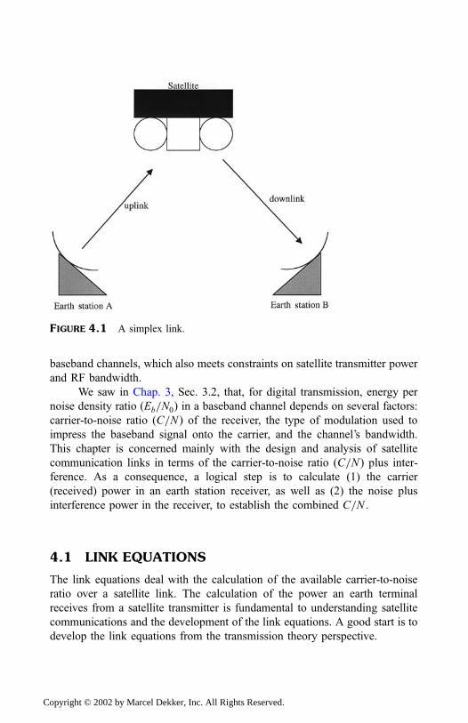
baseband channels, which also meets constraints on satellite transmitter power
and RF bandwidth.
We saw in Chap. 3, Sec. 3.2, that, for digital transmission, energy per
noise density ratio ðEb=N0Þ in a baseband channel depends on several factors:
carrier-to-noise ratio ðC=N Þ of the receiver, the type of modulation used to
impress the baseband signal onto the carrier, and the channel’s bandwidth.
This chapter is concerned mainly with the design and analysis of satellite
communication links in terms of the carrier-to-noise ratio ðC=N Þ plus inter-
ference. As a consequence, a logical step is to calculate (1) the carrier
(received) power in an earth station receiver, as well as (2) the noise plus
interference power in the receiver, to establish the combined C=N .
4.1 LINK EQUATIONS
The link equations deal with the calculation of the available carrier-to-noise
ratio over a satellite link. The calculation of the power an earth terminal
receives from a satellite transmitter is fundamental to understanding satellite
communications and the development of the link equations. A good start is to
develop the link equations from the transmission theory perspective.
FIGURE 4.1 A simplex link.
Copyright © 2002 by Marcel Dekker, Inc. All Rights Reserved.
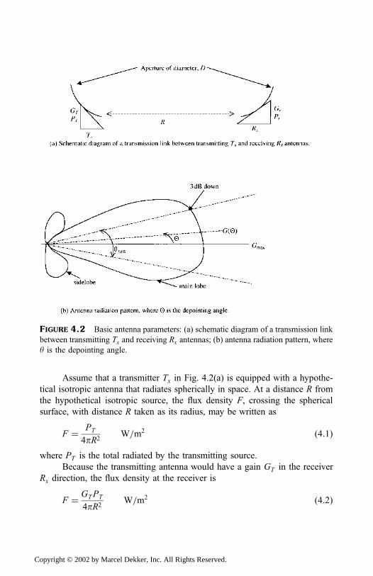
Assume that a transmitter Tx in Fig. 4.2(a) is equipped with a hypothe-
tical isotropic antenna that radiates spherically in space. At a distance R from
the hypothetical isotropic source, the flux density F, crossing the spherical
surface, with distance R taken as its radius, may be written as
F ¼ PT
4pR2W=m2 ð4:1Þ
where PT is the total radiated by the transmitting source.
Because the transmitting antenna would have a gain GT in the receiver
Rx direction, the flux density at the receiver is
F ¼ GTPT
4pR2W=m2 ð4:2Þ
FIGURE 4.2 Basic antenna parameters: (a) schematic diagram of a transmission link
between transmitting Tx and receiving Rx antennas; (b) antenna radiation pattern, where
y is the depointing angle.
Copyright © 2002 by Marcel Dekker, Inc. All Rights Reserved.
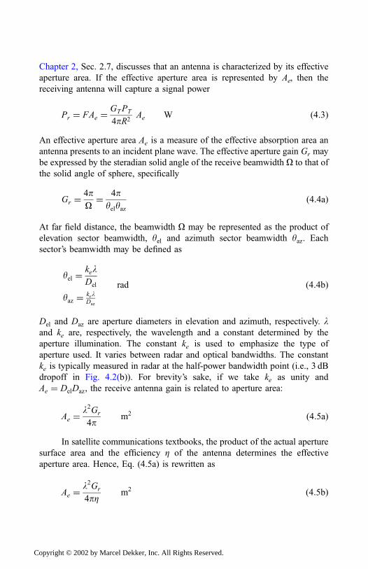
Chapter 2, Sec. 2.7, discusses that an antenna is characterized by its effective
aperture area. If the effective aperture area is represented by Ae, then the
receiving antenna will capture a signal power
Pr ¼ FAe ¼GTPT
4pR2Ae W ð4:3Þ
An effective aperture area Ae is a measure of the effective absorption area an
antenna presents to an incident plane wave. The effective aperture gain Gr may
be expressed by the steradian solid angle of the receive beamwidth O to that of
the solid angle of sphere, specifically
Gr ¼4pO¼ 4p
yelyazð4:4aÞ
At far field distance, the beamwidth O may be represented as the product of
elevation sector beamwidth, yel and azimuth sector beamwidth yaz. Each
sector’s beamwidth may be defined as
yel ¼kelDel
yaz ¼ kelDaz
rad ð4:4bÞ
Del and Daz are aperture diameters in elevation and azimuth, respectively. land ke are, respectively, the wavelength and a constant determined by the
aperture illumination. The constant ke is used to emphasize the type of
aperture used. It varies between radar and optical bandwidths. The constant
ke is typically measured in radar at the half-power bandwidth point (i.e., 3 dB
dropoff in Fig. 4.2(b)). For brevity’s sake, if we take ke as unity and
Ae ¼ DelDaz, the receive antenna gain is related to aperture area:
Ae ¼l2Gr
4pm2 ð4:5aÞ
In satellite communications textbooks, the product of the actual aperture
surface area and the efficiency Z of the antenna determines the effective
aperture area. Hence, Eq. (4.5a) is rewritten as
Ae ¼l2Gr
4pZm2 ð4:5bÞ
Copyright © 2002 by Marcel Dekker, Inc. All Rights Reserved.
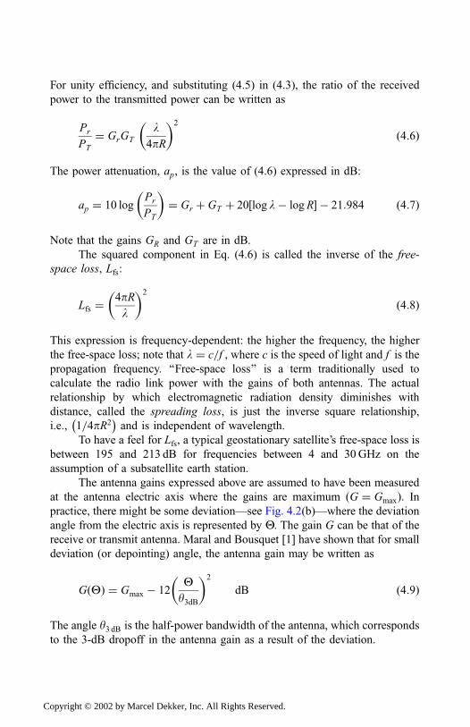
For unity efficiency, and substituting (4.5) in (4.3), the ratio of the received
power to the transmitted power can be written as
Pr
PT
¼ GrGT
l4pR
� �2
ð4:6Þ
The power attenuation, ap, is the value of (4.6) expressed in dB:
ap ¼ 10 logPr
PT
� �¼ Gr þ GT þ 20½log l� logR� � 21:984 ð4:7Þ
Note that the gains GR and GT are in dB.
The squared component in Eq. (4.6) is called the inverse of the free-
space loss, Lfs:
Lfs ¼4pRl
� �2
ð4:8Þ
This expression is frequency-dependent: the higher the frequency, the higher
the free-space loss; note that l ¼ c=f , where c is the speed of light and f is the
propagation frequency. ‘‘Free-space loss’’ is a term traditionally used to
calculate the radio link power with the gains of both antennas. The actual
relationship by which electromagnetic radiation density diminishes with
distance, called the spreading loss, is just the inverse square relationship,
i.e., 1=4pR2� �
and is independent of wavelength.
To have a feel for Lfs, a typical geostationary satellite’s free-space loss is
between 195 and 213 dB for frequencies between 4 and 30GHz on the
assumption of a subsatellite earth station.
The antenna gains expressed above are assumed to have been measured
at the antenna electric axis where the gains are maximum ðG ¼ GmaxÞ. Inpractice, there might be some deviation—see Fig. 4.2(b)—where the deviation
angle from the electric axis is represented by Y. The gain G can be that of the
receive or transmit antenna. Maral and Bousquet [1] have shown that for small
deviation (or depointing) angle, the antenna gain may be written as
GðYÞ ¼ Gmax � 12Yy3dB
� �2
dB ð4:9Þ
The angle y3 dB is the half-power bandwidth of the antenna, which corresponds
to the 3-dB dropoff in the antenna gain as a result of the deviation.
Copyright © 2002 by Marcel Dekker, Inc. All Rights Reserved.
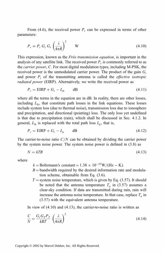
From (4.6), the received power Pr can be expressed in terms of other
parameters:
Pr ¼ Pt Gt Gr
l4pR
� �2
W ð4:10Þ
This expression, known as the Friis transmission equation, is important in the
analysis of any satellite link. The received power Pr is commonly referred to as
the carrier power, C. For most digital modulation types, including M-PSK, the
received power is the unmodulated carrier power. The product of the gain Gt
and power Pt of the transmitting antenna is called the effective isotropic
radiated power (EIRP). Alternatively, we write the received power as
Pr ¼ EIRPþ Gr � Lfs dB ð4:11Þwhere all the terms in the equation are in dB. In reality, there are other losses,
including Lfs, that constitute path losses in the link equations. These losses
include system loss (due to thermal noise), transmission loss due to ionosphere
and precipitation, and directional (pointing) loss. The only loss yet undefined
is that due to precipitation (rain), which shall be discussed in Sec. 4.1.2. In
general, Lfs is replaced with the total path loss Lp, that is,
Pr ¼ EIRPþ Gr � Lp dB ð4:12ÞThe carrier-to-noise ratio C=N can be obtained by dividing the carrier power
by the system noise power. The system noise power is defined in (3.8) as
N ¼ kTB ð4:13Þwhere
k ¼Boltzmann’s constant¼ 1:38� 10�23W=ðHz� KÞ.B¼ bandwidth required by the desired information rate and modula-
tion scheme, obtainable from Eq. (3.6).
T ¼ system noise temperature, which is given by Eq. (3.57). It should
be noted that the antenna temperature Ta in (3.57) assumes a
clear-sky condition. If data are transmitted during rain, rain will
increase the antenna noise temperature. In that case, replace Ta in
(3.57) with the equivalent antenna temperature.
In view of (4.10) and (4.13), the carrier-to-noise ratio is written as
C
N¼ GrGTPT
kBT
l4pR
� �2
ð4:14Þ
Copyright © 2002 by Marcel Dekker, Inc. All Rights Reserved.
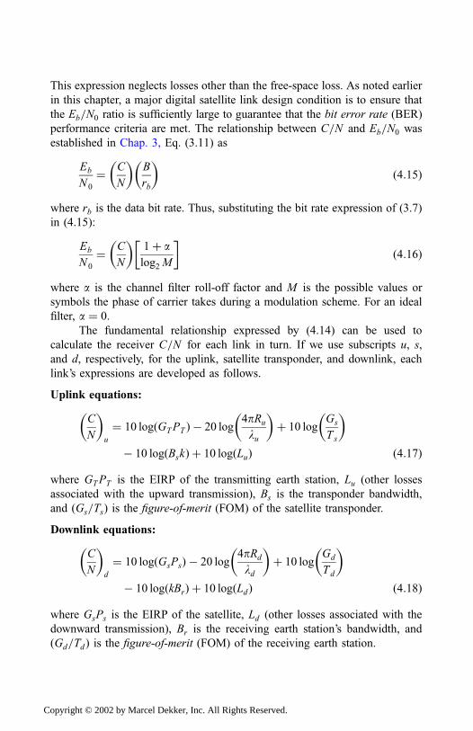
This expression neglects losses other than the free-space loss. As noted earlier
in this chapter, a major digital satellite link design condition is to ensure that
the Eb=N0 ratio is sufficiently large to guarantee that the bit error rate (BER)
performance criteria are met. The relationship between C=N and Eb=N0 was
established in Chap. 3, Eq. (3.11) as
Eb
N 0
¼ C
N
� �B
rb
� �ð4:15Þ
where rb is the data bit rate. Thus, substituting the bit rate expression of (3.7)
in (4.15):
Eb
N 0
¼ C
N
� �1þ alog2 M
� �ð4:16Þ
where a is the channel filter roll-off factor and M is the possible values or
symbols the phase of carrier takes during a modulation scheme. For an ideal
filter, a ¼ 0.
The fundamental relationship expressed by (4.14) can be used to
calculate the receiver C=N for each link in turn. If we use subscripts u, s,
and d, respectively, for the uplink, satellite transponder, and downlink, each
link’s expressions are developed as follows.
Uplink equations:
C
N
� �u
¼ 10 logðGTPT Þ � 20 log4pRu
lu
� �þ 10 log
Gs
Ts
� �� 10 logðBskÞ þ 10 logðLuÞ ð4:17Þ
where GTPT is the EIRP of the transmitting earth station, Lu (other losses
associated with the upward transmission), Bs is the transponder bandwidth,
and ðGs=TsÞ is the figure-of-merit (FOM) of the satellite transponder.
Downlink equations:
C
N
� �d
¼ 10 logðGsPsÞ � 20 log4pRd
ld
� �þ 10 log
Gd
Td
� �� 10 logðkBrÞ þ 10 logðLdÞ ð4:18Þ
where GsPs is the EIRP of the satellite, Ld (other losses associated with the
downward transmission), Br is the receiving earth station’s bandwidth, and
ðGd=TdÞ is the figure-of-merit (FOM) of the receiving earth station.
Copyright © 2002 by Marcel Dekker, Inc. All Rights Reserved.
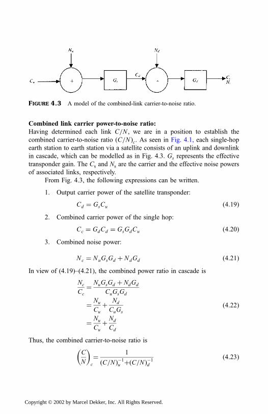
Combined link carrier power-to-noise ratio:
Having determined each link C=N , we are in a position to establish the
combined carrier-to-noise ratio ðC=N Þc. As seen in Fig. 4.1, each single-hop
earth station to earth station via a satellite consists of an uplink and downlink
in cascade, which can be modelled as in Fig. 4.3. Gs represents the effective
transponder gain. The Cs and Ns are the carrier and the effective noise powers
of associated links, respectively.
From Fig. 4.3, the following expressions can be written.
1. Output carrier power of the satellite transponder:
Cd ¼ GsCu ð4:19Þ2. Combined carrier power of the single hop:
Cc ¼ GdCd ¼ GsGdCu ð4:20Þ3. Combined noise power:
Nc ¼ NuGsGd þ NdGd ð4:21ÞIn view of (4.19)–(4.21), the combined power ratio in cascade is
Nc
Cc
¼ NuGsGd þ NdGd
CuGsGd
¼ Nu
Cu
þ Nd
CuGs
¼ Nu
Cu
þ Nd
Cd
ð4:22Þ
Thus, the combined carrier-to-noise ratio is
C
N
� �c
¼ 1
C=Nð Þ�1u þ C=Nð Þ�1d
ð4:23Þ
FIGURE 4.3 A model of the combined-link carrier-to-noise ratio.
Copyright © 2002 by Marcel Dekker, Inc. All Rights Reserved.
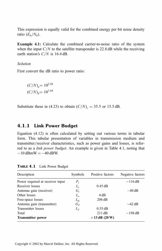
This expression is equally valid for the combined energy per bit noise density
ratio ðEb=N0Þ.
Example 4.1: Calculate the combined carrier-to-noise ratio of the system
when the input C=N to the satellite transponder is 22.8 dB while the receiving
earth station’s C=N is 16.4 dB.
Solution
First convert the dB ratio to power ratio:
C=Nð Þu¼ 102:28
C=Nð Þd¼ 101:64
Substitute these in (4.23) to obtain ðC=N Þc ¼ 35:5 or 15.5 dB.
4.1.1 Link Power Budget
Equation (4.12) is often calculated by setting out various terms in tabular
form. This tabular presentation of variables in transmission medium and
transmitter=receiver characteristics, such as power gains and losses, is refer-
red to as a link power budget. An example is given in Table 4.1, noting that
�10 dBmW¼�40 dBW.
TABLE 4.1 Link Power Budget
Description Symbols Positive factors Negative factors
Power required at receiver input Pr �116 dBReceiver losses Lr 0.45 dB
Antenna gain (receiver) Gr �40 dBOther losses Lo 4 dB
Free-space losses Lfs 206 dB
Antenna gain (transmitter) GT �42 dBTransmitter losses LT 0.55 dB
Total 211 dB �198 dBTransmitter power þ13 dB (20W)
Copyright © 2002 by Marcel Dekker, Inc. All Rights Reserved.
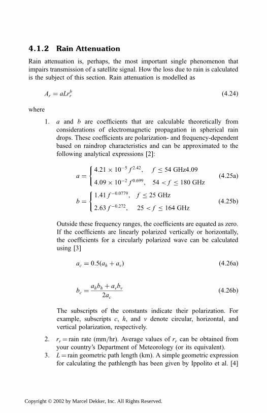
4.1.2 Rain Attenuation
Rain attenuation is, perhaps, the most important single phenomenon that
impairs transmission of a satellite signal. How the loss due to rain is calculated
is the subject of this section. Rain attenuation is modelled as
Ar ¼ aLrbr ð4:24Þ
where
1. a and b are coefficients that are calculable theoretically from
considerations of electromagnetic propagation in spherical rain
drops. These coefficients are polarization- and frequency-dependent
based on raindrop characteristics and can be approximated to the
following analytical expressions [2]:
a ¼4:21� 10�5 f 2:42; f 54 GHz4:09
4:09� 10�2 f 0:699; 54 < f 180 GHz
(ð4:25aÞ
b ¼1:41 f �0:0779; f 25 GHz
2:63 f �0:272; 25 < f 164 GHz
(ð4:25bÞ
Outside these frequency ranges, the coefficients are equated as zero.
If the coefficients are linearly polarized vertically or horizontally,
the coefficients for a circularly polarized wave can be calculated
using [3]
ac ¼ 0:5ðah þ avÞ ð4:26aÞ
bc ¼ahbh þ avbv
2acð4:26bÞ
The subscripts of the constants indicate their polarization. For
example, subscripts c, h, and v denote circular, horizontal, and
vertical polarization, respectively.
2. rr ¼ rain rate (mm=hr). Average values of rr can be obtained from
your country’s Department of Meteorology (or its equivalent).
3. L¼ rain geometric path length (km). A simple geometric expression
for calculating the pathlength has been given by Ippolito et al. [4]
Copyright © 2002 by Marcel Dekker, Inc. All Rights Reserved.
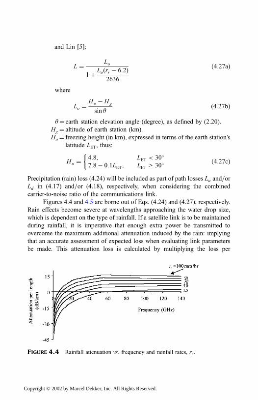
and Lin [5]:
L ¼ Lo
1þ Loðrr � 6:2Þ2636
ð4:27aÞ
where
Lo ¼Ho � Hg
sin yð4:27bÞ
y¼ earth station elevation angle (degree), as defined by (2.20).
Hg ¼ altitude of earth station (km).
Ho¼ freezing height (in km), expressed in terms of the earth station’s
latitude LET, thus:
Ho ¼ 4:8; LET < 30�
7:8� 0:1LET; LET � 30�
ð4:27cÞ
Precipitation (rain) loss (4.24) will be included as part of path losses Lu and=orLd in (4.17) and=or (4.18), respectively, when considering the combined
carrier-to-noise ratio of the communications link.
Figures 4.4 and 4.5 are borne out of Eqs. (4.24) and (4.27), respectively.
Rain effects become severe at wavelengths approaching the water drop size,
which is dependent on the type of rainfall. If a satellite link is to be maintained
during rainfall, it is imperative that enough extra power be transmitted to
overcome the maximum additional attenuation induced by the rain: implying
that an accurate assessment of expected loss when evaluating link parameters
be made. This attenuation loss is calculated by multiplying the loss per
FIGURE 4.4 Rainfall attenuation vs. frequency and rainfall rates, rr.
Copyright © 2002 by Marcel Dekker, Inc. All Rights Reserved.
rainstorm pathlength with the mean pathlength: values that can be extracted
from Figs. 4.4 and 4.5 or alternatively, using expressions (4.24) and (4.27)
after collecting the truth data of the earth station, such as location (latitude,
altitude), orientation (elevation angle), and the average rainfall per hour most
of the year.
Example 4.2: Consider an earth station situated at latitude 5.6�N and at an
altitude of 100m. The Bureau of Meteorology gave the average rainfall of
7.85mm=hr not exceeding 1.09% of the year for the location. If the station is
to be oriented to the satellite at 28.5�, estimate the loss due to rain and the
availability of the link for 12.5-GHz transmission.
Solution
This example brings us to the concepts of outage and availability already
discussed in Chap. 2, Sec. 2.6.5. If PoðArÞ is the percentage of time (also
called percent outage) an attenuation is exceeded, then f1� PoðArÞg is the
percent availability of the link with an attenuation not exceeding Ar. Ar is the
attenuation given by (4.24). Solving this problem:
1. Calculate coefficients a and b using (4.25):
a ¼ 0:01918:
b ¼ 1:1523:
2. Calculate pathlength using (4.27):
L ¼ 9:9759 km:
FIGURE 4.5 Average rainstorm pathlength vs. elevation angle for varying rainfall
rates.
Copyright © 2002 by Marcel Dekker, Inc. All Rights Reserved.
3. Calculate attenuation Ar in dB using (4.24):
Ar ¼ 3:13 dB:
4. Availability
The link can withstand and be available f1� ð1:09%Þg times of the year
if the link design has factored in the effect of rain attenuation. That is, the link
is available 98.91% of the year.
4.2 CARRIER-TO-NOISE PLUS INTERFERENCE RATIO
A transmission source cannot be completely ignored as a potential cause of
interference simply because its primary transmission is out of the operating
band of the satellite links. Interference generated within the transponder can be
a result of one or all of the following:
1. Amplification of multiple carriers by the high-power amplifiers,
which produces intermodulation products and in turn causes strong
interference in other frequency bands.
2. Adjacent channel interference or adjacent transponder interference,
which arises in band-limited satellite channels and may cause
spectrum spreading.
3. A network of earth stations and satellites operating within proximity
of the frequency band, where there is no careful coordination. This
effect is explained as follows, using Fig. 4.6 as a guide.
Suppose that the transmitting earth station (earth station A) radiates a
small percentage of its EIRP toward another satellite (satellite B). Often the
interference generated by an earth station comes from its antenna sidelobes.
This interference signal will appear as noise in the information bandwidth. The
noise and signal in a frequency translating transponder will be amplified and
reradiated to the receiving earth station, B. As a result, the reradiated
interfering uplink and the interfering downlink transmissions combine and
appear as noise in the receiver. It is also possible that satellite B would radiate
some interfering signal to the receiving earth station A, which is receiving
from satellite A. By regulation, this interference is out-of-band and is usually
neglected.
Regulatory agencies (discussed in Chap. 7) provide some guidance on
permissible sidelobes’ envelope level relative to a unity isotropic gain (1 or
0 dB). For example, the U.S. radiocommunications regulator, the Federal
Copyright © 2002 by Marcel Dekker, Inc. All Rights Reserved.
Communications Commission (FCC), specifies the following as permissible
sidelobe envelope levels [6]:
ð29� 25 log yÞ dB 1� a 7�
8 dB 7� a 9:2�
ð32� 25 log yÞ dB 9:2� a 48�
�10 dB 48� a 180�ð4:28Þ
where a is the antenna off-axis (or depointing) angle in degrees. For example
at 6.2�, the sidelobe envelope level must not exceed 9.2 dB above the isotropic
(0-dB) level.
The angular separation between satellites, as seen by the earth stations,
influences the level of interference generated or received from the sidelobe of
the earth station antenna into or from an adjacent satellite. Example 4.3 is
given as an illustration of the influence.
Example 4.3: If the angular separation between two geostationary satellites is
3.45�, and a station-keeping accuracy of � 0.5� is assumed, then the worst-
case viewing angle is 2.95�, which corresponds to the antenna off-axis a of
approximately 3�. Hence, using (4.28), the earth station antenna sidelobes’
envelope level must not exceed 17.1 dB above the isotropic (0-dB) level.
FIGURE 4.6 Adjacent satellite interference.
Copyright © 2002 by Marcel Dekker, Inc. All Rights Reserved.
4.2.1 Intersatellite Links
As indicated earlier in Chap. 2, satellite networks often require communica-
tions between two satellites via an intersatellite link (ISL) as in Fig. 4.6. An
ISL is also called a cross-link. As a communication link, an ISL has the
disadvantage that both transmitter and receiver are spaceborne, thereby limit-
ing operation to both low transmitter power Pt and low figure-of-merit ðG=T Þvalues. For long cross-links, it would be necessary to increase the satellite
EIRP. This means resorting to transmitting with narrow beams to achieve a
higher power concentration. We are constrained by the size of the antenna on
the satellite as such narrow beams can be achieved by transmitting at higher
frequencies. What are the other tradeoffs? The answer will become obvious by
modelling cross-linked satellites as seen in Fig. 4.7.
The two satellites (A and B) in Fig. 4.7 are assumed to know the exact
location of one another, use identical antenna of diameter D and beamwidth fc
pointing at each other, in the same orbit of altitude h, and are not influenced by
any aerodynamic drag.
If the satellites are separated by propagation distance dc and angle gs,and satellite A transmits signal of power Pt to satellite B of equivalent noise
temperature Te, then, by geometry,
dc ¼ 2ðRe þ hÞ sin gs=2� � ð4:29Þ
FIGURE 4.7 A model of an intersatellite link.
Copyright © 2002 by Marcel Dekker, Inc. All Rights Reserved.
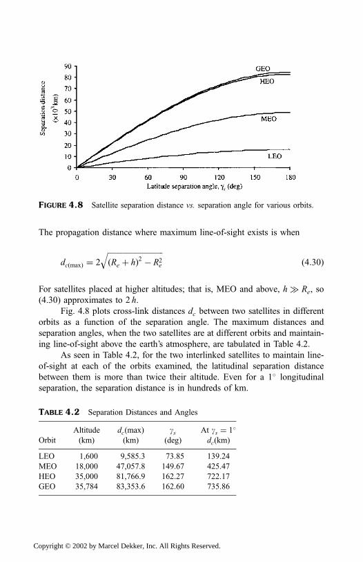
The propagation distance where maximum line-of-sight exists is when
dcðmaxÞ ¼ 2
ffiffiffiffiffiffiffiffiffiffiffiffiffiffiffiffiffiffiffiffiffiffiffiffiffiffiffiffiffiðRe þ hÞ2 � R2
e
qð4:30Þ
For satellites placed at higher altitudes; that is, MEO and above, h� Re, so
(4.30) approximates to 2 h.
Fig. 4.8 plots cross-link distances dc between two satellites in different
orbits as a function of the separation angle. The maximum distances and
separation angles, when the two satellites are at different orbits and maintain-
ing line-of-sight above the earth’s atmosphere, are tabulated in Table 4.2.
As seen in Table 4.2, for the two interlinked satellites to maintain line-
of-sight at each of the orbits examined, the latitudinal separation distance
between them is more than twice their altitude. Even for a 1� longitudinal
separation, the separation distance is in hundreds of km.
FIGURE 4.8 Satellite separation distance vs. separation angle for various orbits.
TABLE 4.2 Separation Distances and Angles
Altitude dcðmaxÞ gs At gs ¼ 1�
Orbit (km) (km) (deg) dc(km)
LEO 1,600 9,585.3 73.85 139.24
MEO 18,000 47,057.8 149.67 425.47
HEO 35,000 81,766.9 162.27 722.17
GEO 35,784 83,353.6 162.60 735.86
Copyright © 2002 by Marcel Dekker, Inc. All Rights Reserved.
We know from (4.4b) that fc is dependent on antenna diameter and
propagation frequency in any sector: that is,
fc lD
ð4:31Þ
This expression assumes that the aperture illumination constant ke equals
unity. We also know that the receiving antenna gain is related to the aperture
area. So, if the antennas are pointing precisely at the desired direction, then
from (4.4a) and (4.5a) we can write the transmitting and receiving satellites’
antenna gain respectively as
Gt ¼4p
f2c
ð4:32aÞ
Gt ¼ 4pAe
l2ð4:32bÞ
The illuminated area Ae is a circle circumscribed by the satellite B antenna of
diameter D; that is, Ae ¼ ðp=4ÞD2. By substituting (4.32) in (4.10), we can
write the carrier-to-noise ratio C=N delivered to the receiving satellite over the
ISL as
C
N¼ pPtD
4
4Nl2d2cð4:33Þ
Since, in practice, satellite cross-links are typically in the K-band in the GHz
frequency range, we can conveniently express the propagation wavelength l asð0:3=f Þ, where f is in GHz. Hence,
C
N¼ 8:73
Pt f2D4
Nd2cð4:34Þ
From this expression, the most practical means of delivering high C=N to the
receiving satellite over ISL is by one of the following because in practice we
are constrained by the size of the antenna that can be deployed:
1. Decreasing the separation distance dc2. Increasing the transmission frequency f
3. Lowering the system front-end noise temperature Te since N is
directly proportional to Te from (3.8)
The limitation of using an extremely narrow concentration of beamwidth
may result in an antenna pointing error due to the inability of satellite A to
accurately locate satellite B. Attitudinal error may also occur; that is, the
Copyright © 2002 by Marcel Dekker, Inc. All Rights Reserved.
inability of satellite A to accurately orient itself quickly enough to point at the
desired direction. These errors are larger than those produced by earth-based
tracking antennas. How then do we quantify the uncertainty angle due to
inaccurate orientation?
If we denote the attitudinal error by fat and the relative location
uncertainty by Dr, we can express the total uncertainty angle as
Y ¼ fat þ180Drpdc
deg ð4:35Þ
This expression implies that the transmitting satellite’s beamwidth must be
wide enough to accommodate these pointing errors. It therefore follows that a
tradeoff exists, either reducing beamwidth fc or improving the pointing
accuracy.
Despite attempts to stabilize the satellites in their orbit, it is difficult to
envision precision pointing every time. It is therefore necessary to consider a
situation where uncertainty can be visualized. If each satellite antenna has
pointing error Y, each antenna’s gain will be a function of GðYÞ, as in (4.9).
Let us denote the transmitting and receiving antenna gain by GtðYtÞ andGrðYrÞ, respectively, and their pointing errors as Yt and Yr, respectively. We
can rewrite C=N delivered at receiving satellite B as
C
N¼ PtGtðYtÞGrðYrÞl2
ð4pÞ2Nd2cð4:36Þ
Upon application of (4.9) in (4.36), the carrier power delivered at the receiving
end can be estimated. Note that the half-power beamwidth, y3 db in (4.9),
equals fc in (4.31).
As noted earlier in this chapter, a major digital satellite link design
condition is to ensure that the Eb=N0 ratio is sufficiently large to guarantee that
the bit error rate (BER) performance criteria are met. From this established
functional relationship between C=N and Eb=N0 , given by Eq. (3.11), and for
an M-PSK system, the decoding Eb=N0 can be written as
Eb
N 0
¼ PtGtðYtÞGrðYrÞl2ð4pÞ2kTed2c rb
ð4:37Þ
where k is the Boltzmann constant (¼ 1.38� 10�23W=Hz-K).Fig 4.9 shows the variation in the data transfer rate with increasing
antenna size for two LEOs maintaining line-of-sight over the earth’s atmo-
sphere, with several transmitter powers, Pt. The antennas are assumed to be
pointing precisely to the desired direction. To have a feel for the data rate that
Copyright © 2002 by Marcel Dekker, Inc. All Rights Reserved.
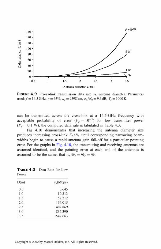
can be transmitted across the cross-link at a 14.5-GHz frequency with
acceptable probability of error (Pe ¼ 10�5) for low transmitter power
ðPt ¼ 0:1 WÞ, the computed data rate is tabulated in Table 4.3.
Fig 4.10 demonstrates that increasing the antenna diameter size
produces increasing cross-link Eb=N0 until corresponding narrowing beam-
widths begin to cause a rapid antenna gain fall-off for a particular pointing
error. For the graphs in Fig. 4.10, the transmitting and receiving antennas are
assumed identical, and the pointing error at each end of the antennas is
assumed to be the same; that is, Yt ¼ Yr ¼ Y.
FIGURE 4.9 Cross-link transmission data rate vs. antenna diameter. Parameters
used: f ¼ 14.5GHz, Z¼ 65%, dc¼ 9598 km, eb=N0¼ 9.6 dB, Te¼ 1000K.
TABLE 4.3 Data Rate for Low
Power
D(m) rb(Mbps)
0.5 0.645
1.0 10.313
1.5 52.212
2.0 156.015
2.5 402.869
3.0 835.390
3.5 1547.663
Copyright © 2002 by Marcel Dekker, Inc. All Rights Reserved.
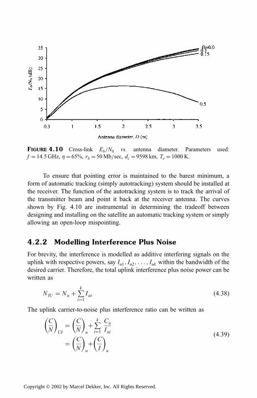
To ensure that pointing error is maintained to the barest minimum, a
form of automatic tracking (simply autotracking) system should be installed at
the receiver. The function of the autotracking system is to track the arrival of
the transmitter beam and point it back at the receiver antenna. The curves
shown by Fig. 4.10 are instrumental in determining the tradeoff between
designing and installing on the satellite an automatic tracking system or simply
allowing an open-loop mispointing.
4.2.2 Modelling Interference Plus Noise
For brevity, the interference is modelled as additive interfering signals on the
uplink with respective powers, say Iu1; Iu2; . . . ; Iuk within the bandwidth of the
desired carrier. Therefore, the total uplink interference plus noise power can be
written as
NIU ¼ Nu þPki¼1
I ui ð4:38Þ
The uplink carrier-to-noise plus interference ratio can be written as
C
N
� �UI
¼ C
N
� �u
þPki¼1
Cu
Iui
¼ C
N
� �u
þ C
I
� �u
ð4:39Þ
FIGURE 4.10 Cross-link Eb=N0 vs. antenna diameter. Parameters used:
f ¼ 14.5GHz, Z¼ 65%, rb¼ 50Mb=sec, dc¼ 9598 km, Te¼ 1000K.
Copyright © 2002 by Marcel Dekker, Inc. All Rights Reserved.
Follow the uplink procedure for the downlink case and consider additive
interfering signals on the downlink with respective powers, say Id1; Id2; . . . ; Idkwithin the bandwidth of the desired carrier. As such, the corresponding carrier-
to-noise plus interference ratio can be written as
C
N
� �DI
¼ C
N
� �d
þPki¼1
Cd
Idi
¼ C
N
� �d
þ C
I
� �d
ð4:40Þ
Thus, the combined carrier-to-noise ratio for a single-hop transmission is
C
N¼ 1
C=Nð Þ�1UIþ C=Nð Þ�1DI
ð4:41Þ
This expression is the most widely used equation in satellite system engineer-
ing. Care must be taken when applying (4.41). For example, when rain occurs
on the downlink only, the carrier-to-noise and interference are attenuated
equally. As such, the downlink carrier-to-interference ratio remains at the
clear-sky value and Eq. (4.40) is used: meaning that the rain attenuation factor
is not included. However, if rain occurs in both uplink and downlink, the effect
of rain-induced attenuation must be included in the link calculation, which is
to further reduce the carrier-to-noise plus interference ratio of the link being
considered.
The overall system quality Eb=N0, the bit energy-to-noise plus inter-
ference density ratio, can be computed from (4.41) and (3.11).
Example 4.4: A satellite system uplink was designed so that the transponder
carrier-to-noise plus interference ratio is 22.5 dB. The link is cascaded with the
downlink for which the receiver carrier-to-noise plus interference ratio is
16.25 dB. Estimate the overall carrier-to-noise ratio of the cascaded link.
Solution
Convert the carrier-to-noise plus interference ratios into power ratio form:
C
N
� �UI
¼ 102:25 ¼ 177:828
and
C
N
� �DI
¼ 101:625 ¼ 42:1697
Copyright © 2002 by Marcel Dekker, Inc. All Rights Reserved.
Then using (4.41), the overall C=N at the cascaded link output becomes
C
N¼ 1
ð177:828Þ�1 þ ð42:1697Þ�1 ¼ 34:087 or 15:33 dB
4.3 SUMMARY
The quality of signals received by the satellite transponder and that retrans-
mitted and received by the receiving earth station are important if successful
information transfer via the satellite is to be achieved. Within constraints of
transmitter power and information channel bandwidth, a communication
system must be designed to meet certain minimum performance standards.
The most important performance standard is the bit energy per noise density
ratio in the information channel, which carries the signals in a format in which
they are delivered to the end users. This chapter explains the process of
designing and calculating the carrier-to-noise ratio as a measure of the system
performance standard.
REFERENCES
1. Maral, G. and Bousquet, M. (1993). Satellite Communications Systems. John
Wiley.
2. Gagliardi, R.M. (1991). Satellite Communications. Van Nostrand Reinhold.
3. Tri, T.H. (1986). Digital Satellite Communications. McGraw-Hill.
4. Ippolito, L.J., Kaul, R.D., and Wallace, R.G. (1986). Propagation effects handbook
for satellite systems design, NASA reference publication 1082(03).
5. Lin, S.H. (1979). Empirical rain attenuation model for earth-satellite path, IEEE
Trans. Communications, 27:5, 812–817.
6. Pritchard, W.L. and Sciulli, J.A. (1986). Satellite Communication Systems Engi-
neering. Prentice-Hall.
PROBLEMS
1. A commercial satellite communication system is to be deployed in an
orbit and is noted to use a 6=4-GHz band. The system has the following
parameters:
Copyright © 2002 by Marcel Dekker, Inc. All Rights Reserved.
Satellite:
Frequencies:
14.75GHz up and
11.36GHz down
Antennas: 1.425� beamwidth up and down (Note that this is 3-dB
measurement.)
Transponder:
Bandwidth¼ 50MHz.
Saturated output power¼ 20.02W.
Input noise temperature¼ 226.5�C.Gain (up to point of saturation)¼ 119.2 dB.
Path losses in benign environment:
201 dB at 14.75GHz
195 dB at 11.36GHz
Earth station:
Antenna:
Diameter 3m
Aperture efficiencies:
64.5% at 1.47GHz 61.25% at 11.36GHz
Ohmic loss between the antenna and LNA¼ 1 dB
Receiver (IF) bandwidth¼ 50MHz.
Calculate the transmitter power required to just saturate the trans-
ponder output amplifier for an earth station at the edge of the
coverage zone of the satellite antenna. Ignoring any noise contri-
butions from the satellite transponder, estimate (i) the earth
station’s G=T required to give a carrier-to-noise ratio of
17.92 dB in the earth station IF amplifier and (ii) the earth station
noise temperature allowing for a loss figure of 0.5 dB.
Find the carrier-to-noise ratio in the transponder when its output is
just saturated. Also find the carrier-to-noise ratio in the earth
receiver IF amplifier when the transponder noise is included.
2. A satellite carrying a 9.8-GHz continuous-wave beacon transmitter is
located in geosynchronous orbit 37,586 km from an earth station. The
beacon’s output power is 0.3Wand feeds an antenna of 19-dB gain toward
the earth station. The antenna is 3.65m in diameter with an aperture
efficiency of 62.5%.
(i) Calculate the satellite EIRP.
(ii) Calculate the receiving antenna gain.
(iii) Calculate the path loss.
Copyright © 2002 by Marcel Dekker, Inc. All Rights Reserved.
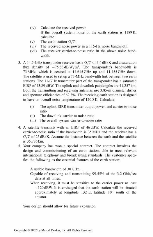
(iv) Calculate the received power.
If the overall system noise of the earth station is 1189K,
calculate
(v) The earth station G=T .(vi) The received noise power in a 115-Hz noise bandwidth.
(vii) The receiver carrier-to-noise ratio in the above noise band-
width.
3. A 14.5-GHz transponder receiver has a G=T of 3.4 dB=K and a saturation
flux density of �75.83 dBW=m2. The transponder’s bandwidth is
73MHz, which is centred at 14.615GHz up and 11.455GHz down.
The satellite is used to set up a 73-MHz bandwidth link between two earth
stations. The 11-GHz transmitter part of the transponder has a saturated
EIRP of 43.89 dBW. The uplink and downlink pathlengths are 41,257 km.
Both the transmitting and receiving antennas use 3.85-m diameter dishes
and aperture efficiencies of 62.3%. The receiving earth station is designed
to have an overall noise temperature of 120.8K. Calculate:
(i) The uplink EIRP, transmitter output power, and carrier-to-noise
ratio
(ii) The downlink carrier-to-noise ratio
(iii) The overall system carrier-to-noise ratio
4. A satellite transmits with an EIRP of 46 dBW. Calculate the received
carrier-to-noise ratio if the bandwidth is 35MHz and the receiver has a
G=T of 25 dB=K. Assume the distance between the earth and the satellite
is 35,786 km.
5. Your company has won a special contract. The contract involves the
design and commissioning of an earth station, able to meet relevant
international telephony and broadcasting standards. The customer speci-
fies the following as the essential features of the earth station:
A usable bandwidth of 30GHz.
Capable of receiving and transmitting 99.55% of the 3.2-Gbit=secdata at all times.
When receiving, it must be sensitive to the carrier power at least
�120 dBW. It is envisaged that the earth station will be situated
approximately at longitude 132�E, latitude 10� south of the
equator.
Your design should allow for future expansion.
Copyright © 2002 by Marcel Dekker, Inc. All Rights Reserved.
6. For link to be maintained between a geosatellite and an earth station about
35,786 km apart, calculate the carrier power (in dB) necessary giving the
following antenna characteristics:
60% efficiency
2.5-cm wavelength
1.3-m diameter transmitting dish
1.0-m diameter receiving dish
To ensure high service quality, it is suggested that the carrier power at the
receiver input must be at least �116 dBW.
7. A satellite transmits with an EIRP of 46 dBW. Calculate the received
carrier-to-noise ratio if the bandwidth is 35MHz and the receiver has a
G=T of 25 dB=K. Assume the distance between the earth and the satellite
is 35,786 km.
8. A broadcast satellite is located in Sydney with the uplinks centred as
20GHz and the downlinks at 12GHz. Calculate the uplink rain attenua-
tion at Brisbane and the downlink attenuation at Melbourne that will not
exceed 99% of the time.
9. A LEO satellite, 1250 km from earth, with a transmitter power of 15W
illuminates a terrestrial circular zone with an approximate radius of
575 km. Calculate the power flux density on the ground in dBW=m2 (i)
for the LEO, (ii) if the satellite is HEO, (iii) if same satellite is positioned
in geostationary orbit. (iv) What advice will you provide a customer
considering positioning a satellite in one of these orbits?
10. A satellite transmits with an EIRP of 46 dBW. Calculate the received
carrier-to-noise ratio if the bandwidth is 35MHz and the receiver has a
G=T of 25 dB=K. Assume the distance between the earth and the satellite
is 35,000 km.
Copyright © 2002 by Marcel Dekker, Inc. All Rights Reserved.
5
Communication Networks andSystems
Communication involves the transfer of information between a source and a
user. Many sources may attempt to transfer information through one satellite
transponder with the result that the available communication capacity of the
transponder is shared among several earth terminals. This sharing technique is
called multiple access (MA). The term access, in satellite transmission
systems, usually refers to multiple access. Sharing can be in many formats,
such as sharing the transponder bandwidth in separate frequency slots
(FDMA), sharing the transponder availability in time slots (TDMA), or
allowing coded signals to overlap in time and frequency (CDMA). The
symbol ‘‘D’’ in the acronym stands for ‘‘division.’’ Division implies switching.
The various transmission switching techniques are discussed in much detail in
this chapter.
Copyright © 2002 by Marcel Dekker, Inc. All Rights Reserved.
5.1 PRINCIPLES OF MULTIPLE ACCESS
As an illustration, consider a satellite transponder of B bandwidth with n
channels as shown in Fig. 5.1. When the transponder is in an operational state
at any time ti, each channel amplifies every carrier fi of the earth terminals ESi(where i ¼ 1; 2; . . . ; n). If no safeguards are in place, it is likely that several
carriers will occupy a particular channel simultaneously and will mutually
interfere.
To avoid such mutual interference, it is important that the receivers of
other earth terminals be able to discriminate among the received carriers.
Discrimination can be achieved by any of three techniques: filtering, temporal
gating, or signature assignment [1].
1. Filtering. Take for instance the carrier energies to be in the frequency
domain. If we subdivide the available channel bandwidth into a number, say n,
as shown in Fig. 5.1, and assign a subchannel to each user upon that user’s
request, then the receiver can discriminate among carriers by filtering. This
multiple-access method is the principle of multiple access by frequency
division (FDMA). It is commonly used in wireline channels to accommodate
multiple users for voice and data transmission.
2. Temporal gating. If, for instance, we subdivide the frame duration Tsinto, say, n nonoverlapping subintervals, each of duration Ts=n, and assign
each user to a particular time slot within each frame, then several carrier
energies can be received sequentially by the receiver. The receiver can thus
FIGURE 5.1 Principle of multiple access.
Copyright © 2002 by Marcel Dekker, Inc. All Rights Reserved.
discriminate among carriers by temporal gating. This multiple-access tech-
nique is the principle of multiple access by time division (TDMA). It is
frequently used in data and digital voice transmission.
It can be observed from the preceding definitions of FDMA and TDMA
that the channel is basically partitioned into independent single-user channels,
that is, nonoverlapping frequency bands or time slots, respectively. FDMA and
TDMA techniques tend to be insufficient in an environment where [2]
1. The transmission from various users is bursty; that is, information
transmission from a single user is separated by periods of silence,
simply no transmission. An example of this case is in digital mobile
cellular communication systems where digitized voice signals
typically contain long pauses,
2. Transmission from several users has a low duty cycle; that is, a
situation where the periods of no transmission are greater than the
periods of transmission.
An alternative to FDMA and TDMA is to allow more than one user to
share a channel or subchannel by use of signature assignment.
3. Signature assignment. This is a process by which a user is assigned a
unique code (or signature) sequence that allows the user to modulate and
spread the information-bearing signal across the assigned frequency band. As
a result, signals from various users can be separated at the receiver by cross
correlation of the received signal with each of the possible user signatures.
This process ensures identification of the carriers even when all the carriers
simultaneously occupy the same frequency band. If the code sequences are
designed to have relatively small cross correlations, then the effect of cross
talk inherent in the demodulation of the signals will be minimized. This
multiple-access technique is the principle of CDMA. Signature assignment is
most often realized by means of pseudo random codes (or pseudo noise
codes), hence the name ‘‘code division multiple access’’ (CDMA). The effect
of using codes is broadening the carrier spectrum in comparison with other
schemes that may have been modulated by the carrier information alone. This
is why CDMA is also called spread-spectrum multiple access (SSMA).
Spreading of the carrier spectrum has an inherent antijam advantage. For
this reason, the designation SSMA is usually used in conjunction with military
systems, whereas CDMA is generally reserved for commercial usage. The
major telecommunication provider in Australia, Telstra, has used CDMA
techniques to provide telecommunication services in rural areas.
An alternative method to CDMA is nonspread random access (NSRA).
In this method, when two users attempt to use a common channel simulta-
Copyright © 2002 by Marcel Dekker, Inc. All Rights Reserved.
neously, their transmissions collide and interfere with each other, resulting in
information loss and possibly requiring retransmission. To avoid retransmis-
sion, protocols are developed for rescheduling transmissions in nonspread
cases. A protocol is a set of necessary procedures or a format that establishes
the timing, instructs the processors, and recognizes the messages.
In essence, depending on the multiplexing and modulation techniques
employed, a range of multiple-access combinations can be derived from these
three basic techniques. The hybrid-access types, for example, could be [3,4]
1. Frequency=time=code division (FD=TD=CDMA)
2. Frequency=time division (FD=TDMA)
3. Time=code division (TD=CDMA)
4. Frequency=code division (FD=CDMA)
It must be recognized that each carrier can employ any modulation
schemes it prefers; for instance, switching or keying the amplitude (ASK),
frequency (FSK), or phase (PSK) of the carrier in accordance with the
information binary digits. To describe a multiple-access system completely,
it is necessary to indicate details of the multiplexing (for instance, frequency
division multiplexer, FDM) and the modulation method (FM) for the channel
group or carrier to be transmitted. A typical designation employed by the
INTELSAT network is FDM-FM-FDMA. The FDM-FM-FDMA utilizes a
multichannel-per-carrier transmission technique. For instance, the transmit-
ting earth station frequency division-multiplexes several single-sideband
suppressed carrier telephone channels into one carrier baseband assembly,
which frequency-modulates an RF carrier and in turn transmits it to an FDMA
satellite transponder.
5.1.1 Frequency Division Multiple Access (FDMA)
The FDMA scheme allows the partitioning of a bandwidth-limited commu-
nication channel into a set of independent lower-speed channels, each of
which uses its permanently assigned portion of the total frequency spectrum
[5]. Each frequency slot contains a unique pair of frequencies needed for
sending its digital signals.
A basic FDMA system is shown in Fig. 5.2, where each uplink earth
station, ESi, in the network transmits one or more carriers at different carrier
frequencies, fi, to the satellite transponder. Each carrier is assigned a frequency
band with a small guard band (or safety zone) to avoid electrically overlapping
Copyright © 2002 by Marcel Dekker, Inc. All Rights Reserved.
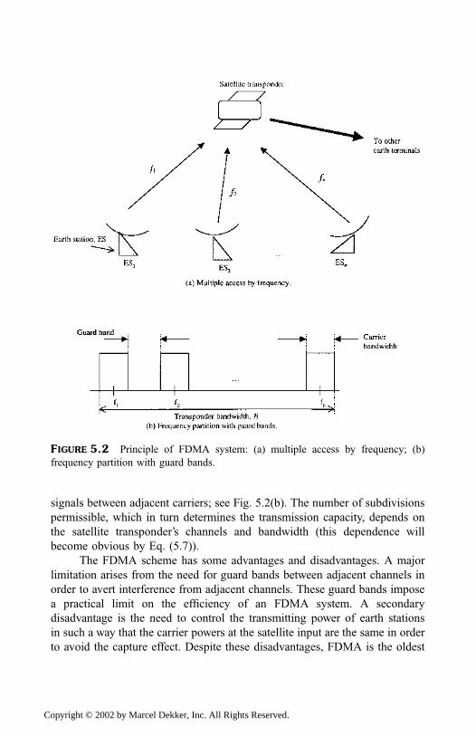
signals between adjacent carriers; see Fig. 5.2(b). The number of subdivisions
permissible, which in turn determines the transmission capacity, depends on
the satellite transponder’s channels and bandwidth (this dependence will
become obvious by Eq. (5.7)).
The FDMA scheme has some advantages and disadvantages. A major
limitation arises from the need for guard bands between adjacent channels in
order to avert interference from adjacent channels. These guard bands impose
a practical limit on the efficiency of an FDMA system. A secondary
disadvantage is the need to control the transmitting power of earth stations
in such a way that the carrier powers at the satellite input are the same in order
to avoid the capture effect. Despite these disadvantages, FDMA is the oldest
FIGURE 5.2 Principle of FDMA system: (a) multiple access by frequency; (b)
frequency partition with guard bands.
Copyright © 2002 by Marcel Dekker, Inc. All Rights Reserved.
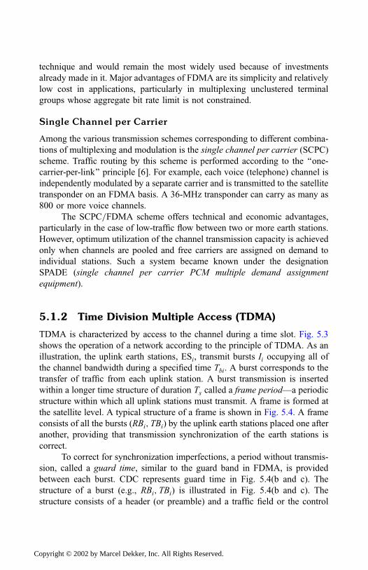
technique and would remain the most widely used because of investments
already made in it. Major advantages of FDMA are its simplicity and relatively
low cost in applications, particularly in multiplexing unclustered terminal
groups whose aggregate bit rate limit is not constrained.
Single Channel per Carrier
Among the various transmission schemes corresponding to different combina-
tions of multiplexing and modulation is the single channel per carrier (SCPC)
scheme. Traffic routing by this scheme is performed according to the ‘‘one-
carrier-per-link’’ principle [6]. For example, each voice (telephone) channel is
independently modulated by a separate carrier and is transmitted to the satellite
transponder on an FDMA basis. A 36-MHz transponder can carry as many as
800 or more voice channels.
The SCPC=FDMA scheme offers technical and economic advantages,
particularly in the case of low-traffic flow between two or more earth stations.
However, optimum utilization of the channel transmission capacity is achieved
only when channels are pooled and free carriers are assigned on demand to
individual stations. Such a system became known under the designation
SPADE (single channel per carrier PCM multiple demand assignment
equipment).
5.1.2 Time Division Multiple Access (TDMA)
TDMA is characterized by access to the channel during a time slot. Fig. 5.3
shows the operation of a network according to the principle of TDMA. As an
illustration, the uplink earth stations, ESi, transmit bursts Ii occupying all of
the channel bandwidth during a specified time Tbi. A burst corresponds to the
transfer of traffic from each uplink station. A burst transmission is inserted
within a longer time structure of duration Ts called a frame period—a periodic
structure within which all uplink stations must transmit. A frame is formed at
the satellite level. A typical structure of a frame is shown in Fig. 5.4. A frame
consists of all the bursts (RBi; TBi) by the uplink earth stations placed one after
another, providing that transmission synchronization of the earth stations is
correct.
To correct for synchronization imperfections, a period without transmis-
sion, called a guard time, similar to the guard band in FDMA, is provided
between each burst. CDC represents guard time in Fig. 5.4(b and c). The
structure of a burst (e.g., RBi; TBi) is illustrated in Fig. 5.4(b and c). The
structure consists of a header (or preamble) and a traffic field or the control
Copyright © 2002 by Marcel Dekker, Inc. All Rights Reserved.
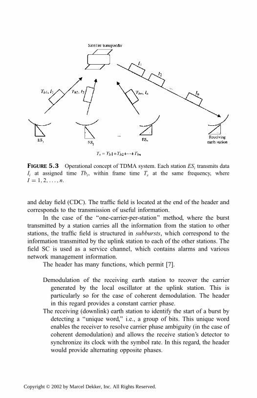
and delay field (CDC). The traffic field is located at the end of the header and
corresponds to the transmission of useful information.
In the case of the ‘‘one-carrier-per-station’’ method, where the burst
transmitted by a station carries all the information from the station to other
stations, the traffic field is structured in subbursts, which correspond to the
information transmitted by the uplink station to each of the other stations. The
field SC is used as a service channel, which contains alarms and various
network management information.
The header has many functions, which permit [7].
Demodulation of the receiving earth station to recover the carrier
generated by the local oscillator at the uplink station. This is
particularly so for the case of coherent demodulation. The header
in this regard provides a constant carrier phase.
The receiving (downlink) earth station to identify the start of a burst by
detecting a ‘‘unique word,’’ i.e., a group of bits. This unique word
enables the receiver to resolve carrier phase ambiguity (in the case of
coherent demodulation) and allows the receive station’s detector to
synchronize its clock with the symbol rate. In this regard, the header
would provide alternating opposite phases.
FIGURE 5.3 Operational concept of TDMA system. Each station ESi transmits data
Ii at assigned time Tbi, within frame time Ts at the same frequency, where
I ¼ 1; 2; . . . ; n.
Copyright © 2002 by Marcel Dekker, Inc. All Rights Reserved.
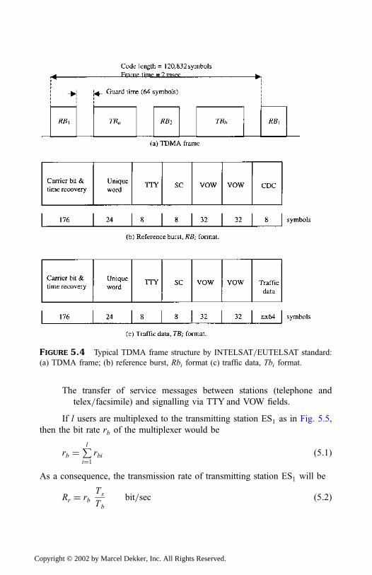
The transfer of service messages between stations (telephone and
telex=facsimile) and signalling via TTY and VOW fields.
If l users are multiplexed to the transmitting station ES1 as in Fig. 5.5,
then the bit rate rb of the multiplexer would be
rb ¼Pli¼1
rbi ð5:1Þ
As a consequence, the transmission rate of transmitting station ES1 will be
Rr ¼ rbTs
Tb
bit=sec ð5:2Þ
FIGURE 5.4 Typical TDMA frame structure by INTELSAT=EUTELSAT standard:
(a) TDMA frame; (b) reference burst, Rbi format (c) traffic data, Tbi format.
Copyright © 2002 by Marcel Dekker, Inc. All Rights Reserved.
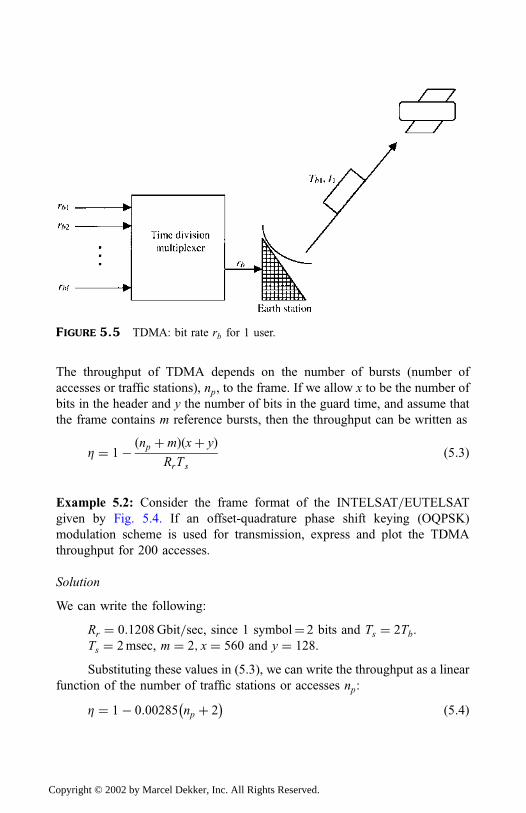
The throughput of TDMA depends on the number of bursts (number of
accesses or traffic stations), np, to the frame. If we allow x to be the number of
bits in the header and y the number of bits in the guard time, and assume that
the frame contains m reference bursts, then the throughput can be written as
Z ¼ 1� ðnp þ mÞðxþ yÞRrTs
ð5:3Þ
Example 5.2: Consider the frame format of the INTELSAT=EUTELSATgiven by Fig. 5.4. If an offset-quadrature phase shift keying (OQPSK)
modulation scheme is used for transmission, express and plot the TDMA
throughput for 200 accesses.
Solution
We can write the following:
Rr ¼ 0:1208Gbit=sec, since 1 symbol¼ 2 bits and Ts ¼ 2Tb.
Ts ¼ 2msec, m ¼ 2; x ¼ 560 and y ¼ 128.
Substituting these values in (5.3), we can write the throughput as a linear
function of the number of traffic stations or accesses np:
Z ¼ 1� 0:00285 np þ 2� � ð5:4Þ
FIGURE 5.5 TDMA: bit rate rb for 1 user.
Copyright © 2002 by Marcel Dekker, Inc. All Rights Reserved.
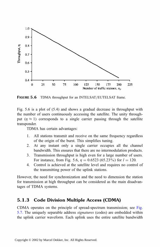
Fig. 5.6 is a plot of (5.4) and shows a gradual decrease in throughput with
the number of users continuously accessing the satellite. The unity through-
put (Z 1) corresponds to a single carrier passing through the satellite
transponder.
TDMA has certain advantages:
1. All stations transmit and receive on the same frequency regardless
of the origin of the burst. This simplifies tuning.
2. At any instant only a single carrier occupies all the channel
bandwidth. This ensures that there are no intermodulation products.
3. Transmission throughput is high even for a large number of users.
For instance, from Fig. 5.6, Z ¼ 0:6523 ð65:23%Þ for l ¼ 120.
4. Control is achieved at the satellite level and requires no control of
the transmitting power of the uplink stations.
However, the need for synchronization and the need to dimension the station
for transmission at high throughput can be considered as the main disadvan-
tages of TDMA systems.
5.1.3 Code Division Multiple Access (CDMA)
CDMA operates on the principle of spread-spectrum transmission; see Fig.
5.7. The uniquely separable address signatures (codes) are embedded within
the uplink carrier waveform. Each uplink uses the entire satellite bandwidth
FIGURE 5.6 TDMA throughput for an INTELSAT=EUTELSAT frame.
Copyright © 2002 by Marcel Dekker, Inc. All Rights Reserved.
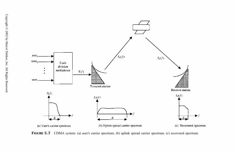
FIGURE 5.7 CDMA system: (a) user’s carrier spectrum; (b) uplink spread carrier spectrum; (c) recovered spectrum.
Copyright ©
2002 by Marcel D
ekker, Inc. All R
ights Reserved.
and transmits through the satellite whenever needed, with all active stations
superimposing their waveforms on the downlink. As such, no time or
frequency separation is required. Carrier separation is achieved at each earth
station by identifying the carrier with the proper signature.
The uplink station, as in Fig. 5.7(b), spreads the user’s spectrum of Fig.
5.7(a). The spread spectrum might contain some noise and other interference
when it is retransmitted. The receiver recovers the useful information by
reducing the spectrum of the carrier transmitted in its original bandwidth, as in
Fig. 5.7(c). The effect of noise and other interference has been suppressed in
Fig. 5.7(c) for brevity. This operation simultaneously spreads the spectrum of
other users in such a way that they appear as noise of low spectral density.
It should be noted that one could not simply use codes of arbitrary
different phases to provide CDMA, because the codes have high-autocorrela-
tion sidelobes at the subsequent periods. Furthermore, the power spectral
density of the codes has line components at frequencies corresponding to each
of the code periods [8].
The spreading ratio is determined primarily by the code ratio kc=rc andcan be achieved either with low-rate channel codes or long address codes,
where
kc ¼ TsB ð5:5Þ
rc ¼1
Tsrbð5:6Þ
Thus, the spreading ratio: kc=rc ¼ B=rb. This ratio is commonly referred to as
the spreading ratio of the code modulation or CDMA bandwidth expansion
factor. In some texts, this ratio is halved because the carrier bandwidth is taken
as B=2.CDMA has some advantages:
1. It is simple to operate.
2. It does not require any transmission synchronization between
stations. The only synchronization required is that of the receiver
to the sequence of the received carrier.
3. It offers sufficient protection against interference from other stations
and that due to multiple paths. This makes CDMA attractive for
networks of small stations with large antenna beamwidths and for
satellite communication with mobiles.
However, on the average, its main disadvantage is the low throughput
demonstrated in the next section.
Copyright © 2002 by Marcel Dekker, Inc. All Rights Reserved.
5.2 CAPACITY COMPARISON OFMULTIPLE-ACCESS METHODS
The capacity of multiple-access (FDMA, TDMA and CDMA) methods can be
examined in terms of the information rate that each method achieves in an
ideal additive white Gaussian noise (AWGN) channel of finite bandwidth B
[9]. For simplicity, we assume a uniform number of users, say l. Each user has
a similar average carrier power Ci ¼ C, for all values of i users where
i ¼ 1; 2; . . . ; l.In FDMA, each user is allocated a bandwidth (B=l). Hence, in view of
(3.10) and (3.19), the capacity for each user can be expressed as
CFD ¼B
llog2 1þ C
B=lð ÞN0
� �ð5:7Þ
Superficially, this expression indicates that for a fixed bandwidth B, the total
capacity goes to infinity as the number of users increases linearly with l. This
is not true, as will be demonstrated later. By writing the carrier power C in
terms of the energy of a single bit Eb as in (3.11), the normalized total capacity
Cn for an FDMA system can be expressed as
Cn ¼ log2 1þ Cn
Eb
N0
� �ð5:8Þ
where Cn ¼ lrb=B, which is the total bit rate for all l users per unit bandwidth
and rb is the input digital bit rate of the user (bit=sec). Alternatively,
Eb
N 0
¼ 2Cn � 1
Cn
ð5:9Þ
Fig. 5.8 shows the graph of Cn versus Eb=N0. We observe that Cn increases as
Eb=NO increases above the minimum value of loge 2, which is the absolute
minimum value, demonstrated by Eq. (3.22), imposed on finite channel
capacity for an error free transmission.
In the TDMA system, each user is allowed to transmit for Ts=l of thetime through the channel of bandwidth B. The total capacity per user can be
expressed as
CTD ¼ BTs
llog2 1þ C
B Ts=l� �
N 0
!ð5:10Þ
This expression is identical to that of the FDMA system in (5.7). In the TDMA
system, however, it may not be possible for the transmitter to sustain an
Copyright © 2002 by Marcel Dekker, Inc. All Rights Reserved.
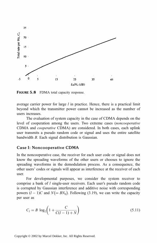
average carrier power for large l in practice. Hence, there is a practical limit
beyond which the transmitter power cannot be increased as the number of
users increases.
The evaluation of system capacity in the case of CDMA depends on the
level of cooperation among the users. Two extreme cases (noncooperative
CDMA and cooperative CDMA) are considered. In both cases, each uplink
user transmits a pseudo random code or signal and uses the entire satellite
bandwidth B. Each signal distribution is Gaussian.
Case I: Noncooperative CDMA
In the noncooperative case, the receiver for each user code or signal does not
know the spreading waveforms of the other users or chooses to ignore the
spreading waveforms in the demodulation process. As a consequence, the
other users’ codes or signals will appear as interference at the receiver of each
user.
For developmental purposes, we consider the system receiver to
comprise a bank of l single-user receivers. Each user’s pseudo random code
is corrupted by Gaussian interference and additive noise with corresponding
powers ðl � 1ÞC and N ¼ BN0
� �. Following (3.19), we can write the capacity
per user as
Cl ¼ B log2 1þ C
Cðl � 1Þ þ N
� �ð5:11Þ
FIGURE 5.8 FDMA total capacity response.
Copyright © 2002 by Marcel Dekker, Inc. All Rights Reserved.
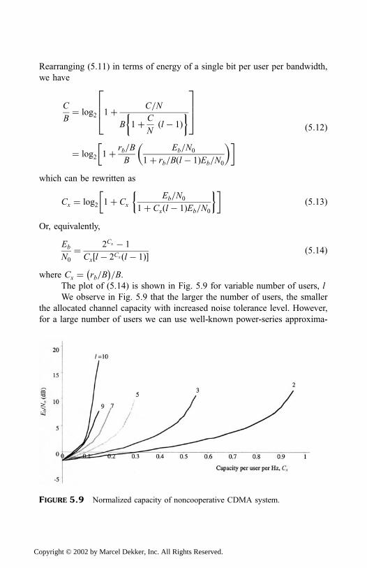
Rearranging (5.11) in terms of energy of a single bit per user per bandwidth,
we have
C
B¼ log2 1þ C=N
B 1þ C
Nðl � 1Þ
2664
3775
¼ log2 1þ rb=B
B
Eb=N0
1þ rb=Bðl � 1ÞEb=N0
� �� � ð5:12Þ
which can be rewritten as
Cx ¼ log2 1þ Cx
Eb=N0
1þ Cxðl � 1ÞEb=N0
� �ð5:13Þ
Or, equivalently,
Eb
N0
¼ 2Cx � 1
Cx l � 2Cx ðl � 1Þ½ � ð5:14Þ
where Cx ¼ rb=B� �
=B.The plot of (5.14) is shown in Fig. 5.9 for variable number of users, l
We observe in Fig. 5.9 that the larger the number of users, the smaller
the allocated channel capacity with increased noise tolerance level. However,
for a large number of users we can use well-known power-series approxima-
FIGURE 5.9 Normalized capacity of noncooperative CDMA system.
Copyright © 2002 by Marcel Dekker, Inc. All Rights Reserved.
tion; that is, logeð1þ xÞ x to estimate the total capacity, where �1 x 1.
In view of (5.13) and upon application of the well-known power-series
approximation, we can write
Cx Cx
Eb=No
1þ Cxðl � 1ÞEb=No
loge ð5:15Þ
Alternatively,
Cx log2 e�1
Eb=N0
1
loge 2� 1
Eb=N0
<1
loge 2
ð5:16Þ
The preceding expressions and Fig. 5.9 show that the total capacity does not
increase with number of users as in FDMA and TDMA systems.
Case II: Cooperative CDMA
In the cooperative CDMA case, the receiver for each user code or signal does
know the spreading waveforms of the other users. As a consequence, the
system receiver comprising a bank of l single-user receivers knows all l users’
spreading waveforms and jointly detects and demodulates all users’ codes. If
we assign each user
A transmission rate Rri (where i ¼ 1; 2; . . . ; l)A codebook containing a set of 2kðLc�1Þ
� �) codewords* of carrier power
CI (where k ¼ number of input bits and Lc¼ constraint lengthy)
then the achievable l-dimensional rate region for the l users may be
represented by
Rr ¼Pli¼1
Rri < B log2 1þ lCi
N
� �ð5:17Þ
Note that this expression assumes equal carrier power Ci ¼ C for each user.
*A codeword is the number of bits transmitted in a block. For example, if we transmit n bits in ablock, which is made up of k message bits plus r parity check bits, then the n-bit block is called acodeword.y Constraint length is defined as the number of shifts over which a single message bit can influencethe encoder output. This definition becomes clearer in Chap. 6.
Copyright © 2002 by Marcel Dekker, Inc. All Rights Reserved.
The transmission bit rate is
Rr ¼ rbTs
Tb
bit=sec ð5:18Þ
where
rb¼ input digital bit rate of the user (bit=sec).Ts¼ symbol (or frame) duration (sec).
Tb¼ bit (or burst) duration (sec).
It follows from this expression that if the rates Rri were selected to fall
within the specified capacity region, the probabilities of errorsz for l users tendto zero as the code block length, b, tends to infinity. Suffice to say that the sum
of the rates tends to infinity with l users. In this instance, the cooperative
CDMA has a similar format as the FDMA and TDMA.
Further comparison with FDMA and TDMA systems shows that if all
the rates in the CDMA are selected to be identical, than (5.17) reduces to
Rr < B log2 1þ lCi
N
� �ð5:19Þ
which incidentally is identical to the constraint applied to TDMA and FDMA;
note that N ¼ BN0 and lCi is the total carrier power for all the users. We
conclude that if the aggregated rates are unequally selected, there exists a point
where the rates in the CDMA system exceed the capacity of FDMA and
TDMA. This point will be fun for the reader to establish.
5.3 SUMMARY
This chapter has discussed the techniques that permit several earth terminals or
stations on the same network to exchange information via a nodal point that
the satellite represents. These techniques are FDMA, TDMA, and CDMA:
they exploit the geometric advantage created by the use of the satellite.
Comparisons between the capacity of these multiple-access methods are
examined in terms of the information rate that each method achieves in an
ideal ‘‘additive white Gaussian noise’’ channel of finite bandwidth.
zAs defined in Chap. 3, Eq. (3.12).
Copyright © 2002 by Marcel Dekker, Inc. All Rights Reserved.
REFERENCES
1. Spilker, J.J. (1977). Digital Communications by Satellite. Prentice-Hall.
2. Puente, J.G. and Werth, A.M. (1974). Demand-assigned service for the Intelsat
Global Network, IEEE Spectrum, vol. 8:1, 59–69.
3. Gargliardi, R.M. (1991). Satellite Communications. Van Nostrand Reinhold.
4. Tri, T.H. (1986). Digital Satellite Communications. McGraw-Hill.
5. Frenkel, G. (1974). The grade of service in multiple-access satellite communica-
tions systems with demand assignments, IEEE Trans. Communications, COM-22
1681–1685.
6. Maral, G. and Bousquet, M. (1993). Satellite Communications Systems. JohnWiley.
7. CCIR-1988.
8. Viterbi, A.J (1995). CDMA: Principles of Spread Spectrum Communication.
Addison-Wesley.
9. Shannon, C.E. (1948). A mathematical theory of communication, Bell System Tech
J., vol. 27.
PROBLEMS
1. What does the phrase ‘‘access to a communication satellite’’ mean?
2. Explain the principle behind the following schemes: FDMA, CDMA, and
TDMA. Is it operationally possible to have a combination of these
schemes? Give examples.
3. A TDMA slot acquisition system uses a frequency burst of 20 ms to
determine its range. The satellite has a 500-MHz bandwidth and can
produce a 10-dB downlink carrier. How much lower in power can the
frequency burst be, relative to a TDMA carrier, to produce the same carrier-
to-noise ratio in its filter bandwidth?
4. A QPSK TDMA system is to transmit 10,000 digital voice channels. Each
channel has four bits per sample at a rate of 64 kb=sec. The system is
envisioned to accommodate 100 data bits=slot, at a frame efficiency of
15%. Determine
(i) The satellite bandwidth required
(ii) The number of slots per frame
(iii) The number of preamble bits to be used
5. In an FDMA system, frequency band selection may be fixed or assigned
when demanded. Describe the difference between these two schemes. What
action must be taken to prevent carrier cross talk?
Copyright © 2002 by Marcel Dekker, Inc. All Rights Reserved.
6
Error Detection and CorrectionCoding Schemes
Coding techniques are used for several reasons: reduction of dc wandering,
suppression of intersymbol interference, and self-clocking capability. These
problems are of engineering interest in the transmission of digital data. The
coding schemes discussed in this chapter are for error detection and correction,
specifically forward error correction (FEC) techniques. FEC codes may be
divided into two classes of codes, namely, linear block codes and convolu-
tional codes [1]. Depending on the intended use of codes, FEC enables the
receiver not only to detect errors but also to facilitate their correction.
To enhance the reader’s understanding of the subject matter, we briefly
introduce the principle of channel coding, followed by coding and decoding
schemes. This arrangement enables the reader to move on to concrete
realizations without great difficulty.
Copyright © 2002 by Marcel Dekker, Inc. All Rights Reserved.
6.1 CHANNEL CODING
Noise within a transmission channel inevitably causes discrepancies or errors
between the channel input and channel output. A channel is a specific portion
of the information-carrying capacity of a network interface specified by a
certain transmission rate. In Chap. 3, Sec. 3.2.5, and Chap. 5, Sec. 5.2, the
concepts of bit error rate and channel capacity using Shannon’s theorem were
respectively discussed in some detail [2].
Coding enables the receiver to decode the incoming coded signals not
only to detect errors but also to correct them. Effectively encoding signals
from discrete sources and approximating a specified Shannon limit are
achievable by symbol combination in large blocks and by the application of
special coding methods such as Huffman [3] codes and Fano1 [4] codes. For
clarification, the terms ‘‘data compression’’ and ‘‘effective encoding’’ are
treated as synonyms: meaning that redundancy is eliminated from the original
signal, and it is then encoded as economically as possible with a minimum
number of binary symbols [5]. An encoder performs redundancy elimination.
The application of the effective encoding methods essentially reduces the
required channel transmission rate.
In general, if k binary digits enter the channel encoder, and the channel
encoder outputs n binary digits, then the code rate can be defined as
Rc ¼k
nð6:1Þ
The channel-coding theorem specifies the capacity Cc as a fundamental limit
on the rate at which the transmission of reliable errorfree message can take
place over a discrete memoryless channel (DMC). The concept of DMC has
been discussed in Chap. 3. For example, let a discrete memoryless source with
an alphabet X have entropy HðX Þ and produce one symbol every Ts sec.
Supposing that a DMC with capacity Cc (bit=symbol) is used once every Tcsec; then if
HðX ÞTs Cc
Tcð6:2Þ
there exists a coding scheme for which the source output can be transmitted
over the channel and be retrieved and reconstructed with an arbitrarily small
probability of error. Conversely, it is impossible to transfer information over
1 Also called Shannon–Fado codes.
Copyright © 2002 by Marcel Dekker, Inc. All Rights Reserved.
the channel and reconstruct the source signal with an arbitrarily small
probability of error if
HðX ÞTs
>Cc
Tcð6:3Þ
The parameter Cc=Tc is called the critical rate. When HðX Þ=Ts ¼ Cc=Tc, thesystem is said to be operating at the critical rate (at capacity). Fig. 5.8 (in
Chap. 5, Sec. 5.2) has demonstrated that operating a system at capacity is
achievable only if the value of Eb=N0 is above the Shannon limit; that is,
loge 2ð�1:6 dBÞ. Recently, however, parallel-concatenated convolutional codes
have achieved a performance close to this theoretical limit [6] (more is said of
the convolutional coding technique in Sec. 6.2.2). In general, the objective is
to achieve maximum data transfer in a minimum bandwidth while maintaining
an acceptable quality of transmission. To achieve this, an error-detecting code
must be devised. The most desirable solution is to use a forward error
correction (FEC) technique. Error detection coding is a technique for
adding redundant (extra) bits to a data stream in such a way that an error in
the data stream can be detected [7].
6.2 FORWARD ERROR CORRECTION CODINGTECHNIQUES
Forward error correction (FEC) techniques are widely used in control and
telecommunication systems. FEC codes may be divided into two broad types:
linear block codes and convolutional codes.
6.2.1 Linear Block Codes
In linear block codes, the encoder splits up (or maps) the incoming data stream
into blocks of k digits and processes each block individually by adding
redundancy (extra digits) as a parity check according to a predefined algo-
rithm. The output of the encoder is a codeword with n digits, where n > k. The
code rate is also given by (6.1).
The general form of a linear block codeword is
Y ¼ GX ð6:4Þ
Copyright © 2002 by Marcel Dekker, Inc. All Rights Reserved.
where G is a generator matrix that creates the check bits from the data bits,
while the input message vector X and code (output) vector Y have components
defined as
X ¼ ðx1; x2; x3; . . . ; xkÞY ¼ ðy1; y2; y3; . . . ; ynÞ
ð6:5Þ
From elementary mathematics, multiplication of matrices can be performed
only when the number of columns in Y equals the number of rows in matrix X .
Hence the generator matrix G will have k rows by n columns:
G ¼g11 g12 � � � g1ng21 g22 � � � g2n
..
. ... � � � ..
.
gk1 gk2 � � � gkn
26664
37775 ð6:6Þ
The addition that occurs in the matrix multiplication is mod-2 arithmetic; this
becomes clearer in the example that follows.
Example 6.1: Consider message data X to be a 2-bit data word [8] and the
generator matrix is
G ¼ 1 0 1
0 1 1
� �ð6:7aÞ
Then the codeword Y is
Y ¼ 1 0 1
0 1 1
� �½1 0�
¼ ½ð1� 1Þ � ð0� 0Þ�½ð1� 0Þ � ð0� 1Þ�½ð1� 1Þ � ð0� 1Þ�¼ ð1� 0Þð0� 0Þð1� 0Þ¼ 101
ð6:7bÞ
Thus, Y is a (3, 2) codeword having two data bits and one parity bit.
The process of code design is the process of determining the elements of
the generator matrix. The subject of code design is involved, and the interested
reader should consult Lin and Costello [9] for a detailed treatment of the
subject and Shamnugam [10] for a review of coding for communication
purposes.
Without loss of generality, the code in Example 6.1 can be considered
systematic. A code is systematic if the first k bits of codeword Y constitute the
Copyright © 2002 by Marcel Dekker, Inc. All Rights Reserved.
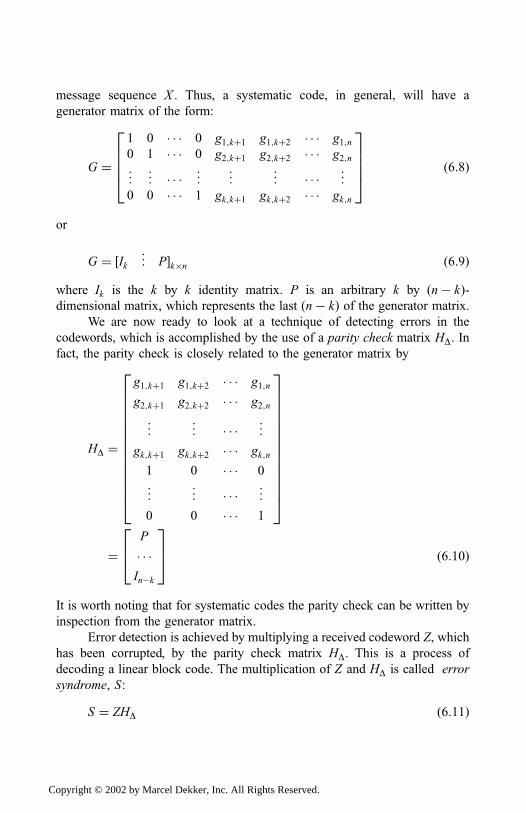
message sequence X . Thus, a systematic code, in general, will have a
generator matrix of the form:
G ¼
1 0 � � � 0 g1;kþ1 g1;kþ2 � � � g1;n0 1 � � � 0 g2;kþ1 g2;kþ2 � � � g2;n
..
. ... � � � ..
. ... ..
. � � � ...
0 0 � � � 1 gk;kþ1 gk;kþ2 � � � gk;n
26664
37775 ð6:8Þ
or
G ¼ ½Ik ...
P�k�n ð6:9Þwhere Ik is the k by k identity matrix. P is an arbitrary k by ðn� kÞ-dimensional matrix, which represents the last ðn� kÞ of the generator matrix.
We are now ready to look at a technique of detecting errors in the
codewords, which is accomplished by the use of a parity check matrix HD. In
fact, the parity check is closely related to the generator matrix by
HD ¼
g1;kþ1 g1;kþ2 � � � g1;n
g2;kþ1 g2;kþ2 � � � g2;n
..
. ... � � � ..
.
gk;kþ1 gk;kþ2 � � � gk;n
1 0 � � � 0
..
. ... � � � ..
.
0 0 � � � 1
266666666666664
377777777777775
¼P
� � �In�k
264
375 ð6:10Þ
It is worth noting that for systematic codes the parity check can be written by
inspection from the generator matrix.
Error detection is achieved by multiplying a received codeword Z, which
has been corrupted, by the parity check matrix HD. This is a process of
decoding a linear block code. The multiplication of Z and HD is called error
syndrome, S:
S ¼ ZHD ð6:11Þ
Copyright © 2002 by Marcel Dekker, Inc. All Rights Reserved.
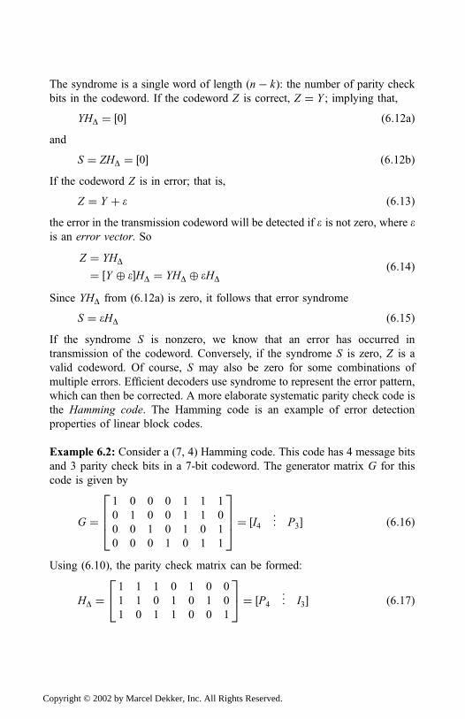
The syndrome is a single word of length (n� k): the number of parity check
bits in the codeword. If the codeword Z is correct, Z ¼ Y ; implying that,
YHD ¼ ½0� ð6:12aÞand
S ¼ ZHD ¼ ½0� ð6:12bÞIf the codeword Z is in error; that is,
Z ¼ Y þ e ð6:13Þthe error in the transmission codeword will be detected if e is not zero, where eis an error vector. So
Z ¼ YHD
¼ ½Y � e�HD ¼ YHD � eHDð6:14Þ
Since YHD from (6.12a) is zero, it follows that error syndrome
S ¼ eHD ð6:15ÞIf the syndrome S is nonzero, we know that an error has occurred in
transmission of the codeword. Conversely, if the syndrome S is zero, Z is a
valid codeword. Of course, S may also be zero for some combinations of
multiple errors. Efficient decoders use syndrome to represent the error pattern,
which can then be corrected. A more elaborate systematic parity check code is
the Hamming code. The Hamming code is an example of error detection
properties of linear block codes.
Example 6.2: Consider a (7, 4) Hamming code. This code has 4 message bits
and 3 parity check bits in a 7-bit codeword. The generator matrix G for this
code is given by
G ¼1 0 0 0 1 1 1
0 1 0 0 1 1 0
0 0 1 0 1 0 1
0 0 0 1 0 1 1
2664
3775 ¼ ½I4 ..
.P3� ð6:16Þ
Using (6.10), the parity check matrix can be formed:
HD ¼1 1 1 0 1 0 0
1 1 0 1 0 1 0
1 0 1 1 0 0 1
24
35 ¼ ½P4
..
.I3� ð6:17Þ
Copyright © 2002 by Marcel Dekker, Inc. All Rights Reserved.
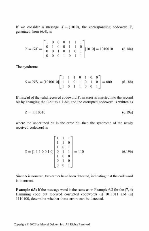
If we consider a message X ¼ ð1010Þ, the corresponding codeword Y,
generated from (6.4), is
Y ¼ GX ¼1 0 0 0 1 1 1
0 1 0 0 1 1 0
0 0 1 0 1 0 1
0 0 0 1 0 1 1
2664
3775½1010� ¼ 1010010 ð6:18aÞ
The syndrome
S ¼ YHD ¼ ½1010010�1 1 1 0 1 0 0
1 1 0 1 0 1 0
1 0 1 1 0 0 1
24
35 ¼ 000 ð6:18bÞ
If instead of the valid received codeword Y, an error is inserted into the second
bit by changing the 0-bit to a 1-bit, and the corrupted codeword is written as
Z ¼ 1110010 ð6:19aÞ
where the underlined bit is the error bit, then the syndrome of the newly
received codeword is
S ¼ ½1 1 1 0 0 1 0�
1 1 1
1 1 0
1 0 1
0 1 1
1 0 0
0 1 0
0 0 1
2666666664
3777777775¼ 110 ð6:19bÞ
Since S is nonzero, two errors have been detected, indicating that the codeword
is incorrect.
Example 6.3: If the message word is the same as in Example 6.2 for the (7, 4)
Hamming code but received corrupted codewords (i) 1011011 and (ii)
1110100, determine whether these errors can be detected.
Copyright © 2002 by Marcel Dekker, Inc. All Rights Reserved.
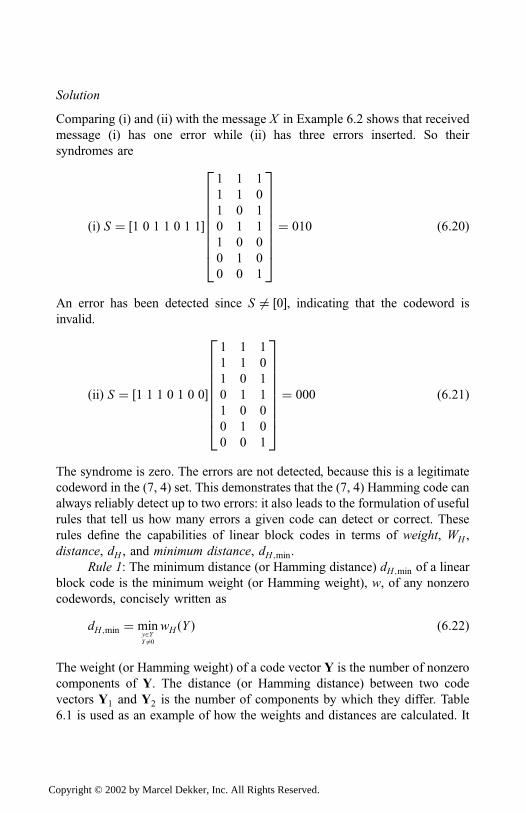
Solution
Comparing (i) and (ii) with the message X in Example 6.2 shows that received
message (i) has one error while (ii) has three errors inserted. So their
syndromes are
ðiÞ S ¼ ½1 0 1 1 0 1 1�
1 1 1
1 1 0
1 0 1
0 1 1
1 0 0
0 1 0
0 0 1
2666666664
3777777775¼ 010 ð6:20Þ
An error has been detected since S 6¼ ½0�, indicating that the codeword is
invalid.
ðiiÞ S ¼ ½1 1 1 0 1 0 0�
1 1 1
1 1 0
1 0 1
0 1 1
1 0 0
0 1 0
0 0 1
2666666664
3777777775¼ 000 ð6:21Þ
The syndrome is zero. The errors are not detected, because this is a legitimate
codeword in the (7, 4) set. This demonstrates that the (7, 4) Hamming code can
always reliably detect up to two errors: it also leads to the formulation of useful
rules that tell us how many errors a given code can detect or correct. These
rules define the capabilities of linear block codes in terms of weight, WH ,
distance, dH , and minimum distance, dH;min.
Rule 1: The minimum distance (or Hamming distance) dH;min of a linear
block code is the minimum weight (or Hamming weight), w, of any nonzero
codewords, concisely written as
dH;min ¼ miny2YY 6¼0
wH ðY Þ ð6:22Þ
The weight (or Hamming weight) of a code vector Y is the number of nonzero
components of Y. The distance (or Hamming distance) between two code
vectors Y1 and Y2 is the number of components by which they differ. Table
6.1 is used as an example of how the weights and distances are calculated. It
Copyright © 2002 by Marcel Dekker, Inc. All Rights Reserved.
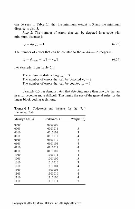
can be seen in Table 6.1 that the minimum weight is 3 and the minimum
distance is also 3.
Rule 2: The number of errors that can be detected in a code with
minimum distance is
nd ¼ dH;min � 1 ð6:23Þ
The number of errors that can be counted to the next-lowest integer is
nc ¼ dH;min � 1=2 ¼ nd=2 ð6:24Þ
For example, from Table 6.1:
The minimum distance dH;min ¼ 3:The number of errors that can be detected nd ¼ 2.
The number of errors that can be counted nc ¼ 1.
Example 6.3 has demonstrated that detecting more than two bits that are
in error becomes more difficult. This limits the use of the general rules for the
linear block coding technique.
TABLE 6.1 Codewords and Weights for the (7,4)
Hamming Code
Message bits, X Codeword, Y Weight, wH
0000 0000000 —
0001 0001011 3
0010 0010101 3
0011 0011110 4
0100 0100110 3
0101 0101101 4
0110 0110011 4
0111 0111000 3
1000 1000111 4
1001 1001100 3
1010 1010010 3
1011 1011001 4
1100 1100001 3
1101 1101010 4
1110 1110100 4
1111 1111111 7
Copyright © 2002 by Marcel Dekker, Inc. All Rights Reserved.
Cyclic Codes
Cyclic codes are a subset of linear block codes. They are the most useful and
popular because encoding and decoding can be implemented by using simple
shift registers: error detection and correction are achieved with shift registers
and some additional logic gates. With a cyclic code, an end-around shift of a
codeword yields another codeword. For example, if
ðy1; y2; y3; � � � ; yn�1; ynÞis a codeword, then, by definition, a cyclic code is also a codeword of the form
ðyn; y1; y2; y3; � � � ; yn�1ÞIt follows from the above cyclic code description that only n� 1 codewords
can be generated by cyclic shifts of a single codeword.
Encoding is achieved by using either an ðn� kÞ-stage shift register or ak-stage shift register. Syndrome calculation for decoding is achieved by an
ðn� kÞ-stage shift register or a k-stage shift register. An example of encoding
and decoding of a cyclic code is shown in Fig. 6.1.
Fig. 6.1(a) is a (7, 4) encoder. It generates a 7-bit codeword using a 3-
shift register ðr0; r1; r2Þ. The message bits form the first 4 bits of the 7-bit
codeword. When the gate is closed and the output switch is set to position 1,
the most significant bits of the message bits are transmitted first. As the 4
message bits are transmitted, the gate is opened, allowing the data bits to be
shifted into the 3-shift register. After the 4 bits have been transmitted and fed
into the shift register, the output switch is set to position 2. The contents of the
shift register are then transmitted, forming the 3 parity check bits.
The output buffer from the encoder is the 7-bit-long codeword, which is
fed into the syndrome forming part of the decoder in Fig. 6.1(b). The
syndrome output is AND-gated, acting as the error detector. The AND gate
gives a binary ‘‘1’’ output only when the AND input equals 100. If the AND
output is ‘‘0,’’ the current bit in the received codeword is correct and the
received sequence is then shifted out of the decoder.
Cyclic codes have rich algebraic properties, which allow for efficient
decoding techniques. A number of books, including Peterson [11], Lin and
Costello [9], and Shamnugam [10], have provided excellent mathematical
treatment of cyclic codes that inquiring readers should consult.
BCH Codes
The BCH (Bose–Chaudhuri–Hocquenghem) codes [12] are perhaps the most
powerful and flexible group of cyclic error correction codes available. Their
Copyright © 2002 by Marcel Dekker, Inc. All Rights Reserved.
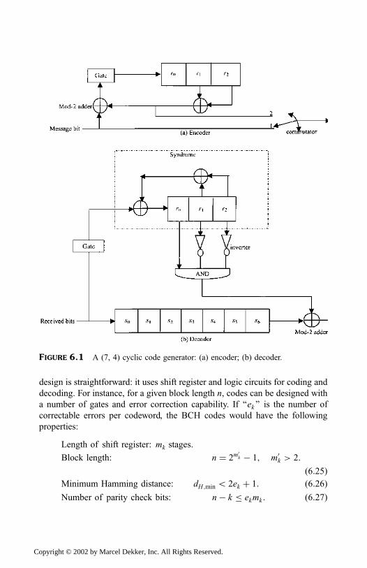
design is straightforward: it uses shift register and logic circuits for coding and
decoding. For instance, for a given block length n, codes can be designed with
a number of gates and error correction capability. If ‘‘ek’’ is the number of
correctable errors per codeword, the BCH codes would have the following
properties:
Length of shift register: mk stages:
Block length: n ¼ 2m0k � 1; m0k > 2:
ð6:25ÞMinimum Hamming distance: dH;min 5 2ek þ 1: ð6:26ÞNumber of parity check bits: n� k ekmk : ð6:27Þ
FIGURE 6.1 A (7, 4) cyclic code generator: (a) encoder; (b) decoder.
Copyright © 2002 by Marcel Dekker, Inc. All Rights Reserved.
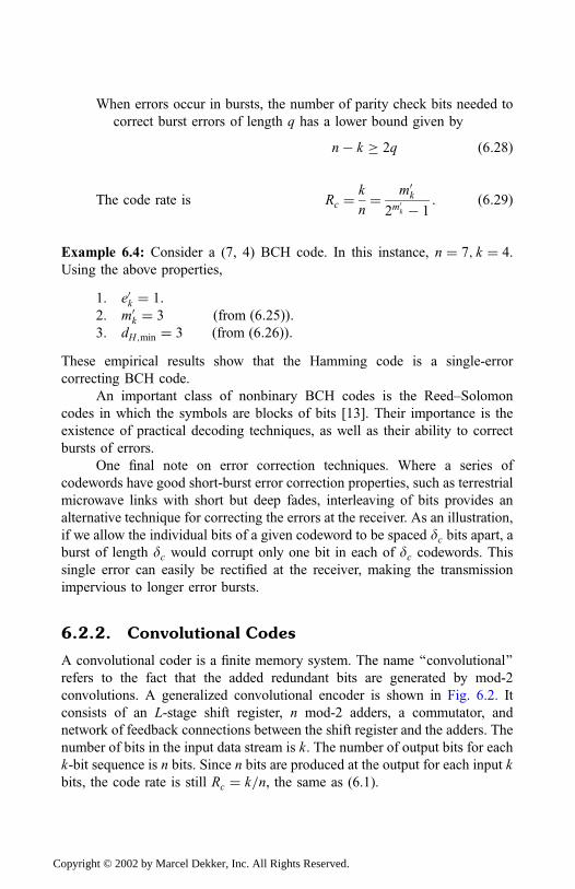
When errors occur in bursts, the number of parity check bits needed to
correct burst errors of length q has a lower bound given by
n� k � 2q ð6:28Þ
The code rate is Rc ¼k
n¼ m0k
2m0k � 1
: ð6:29Þ
Example 6.4: Consider a (7, 4) BCH code. In this instance, n ¼ 7; k ¼ 4.
Using the above properties,
1. e0k ¼ 1:2. m0k ¼ 3 ðfrom ð6:25ÞÞ:3. dH;min ¼ 3 ðfrom ð6:26ÞÞ:
These empirical results show that the Hamming code is a single-error
correcting BCH code.
An important class of nonbinary BCH codes is the Reed–Solomon
codes in which the symbols are blocks of bits [13]. Their importance is the
existence of practical decoding techniques, as well as their ability to correct
bursts of errors.
One final note on error correction techniques. Where a series of
codewords have good short-burst error correction properties, such as terrestrial
microwave links with short but deep fades, interleaving of bits provides an
alternative technique for correcting the errors at the receiver. As an illustration,
if we allow the individual bits of a given codeword to be spaced dc bits apart, aburst of length dc would corrupt only one bit in each of dc codewords. Thissingle error can easily be rectified at the receiver, making the transmission
impervious to longer error bursts.
6.2.2. Convolutional Codes
A convolutional coder is a finite memory system. The name ‘‘convolutional’’
refers to the fact that the added redundant bits are generated by mod-2
convolutions. A generalized convolutional encoder is shown in Fig. 6.2. It
consists of an L-stage shift register, n mod-2 adders, a commutator, and
network of feedback connections between the shift register and the adders. The
number of bits in the input data stream is k. The number of output bits for each
k-bit sequence is n bits. Since n bits are produced at the output for each input k
bits, the code rate is still Rc ¼ k=n, the same as (6.1).
Copyright © 2002 by Marcel Dekker, Inc. All Rights Reserved.
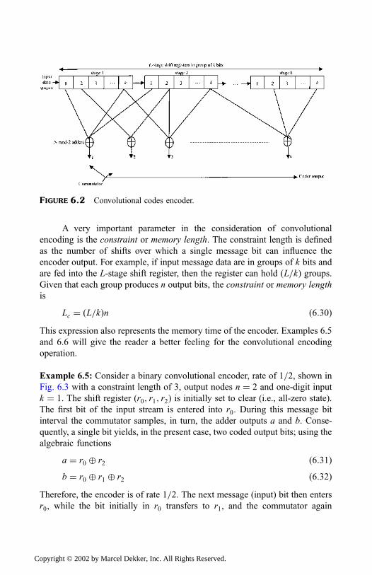
A very important parameter in the consideration of convolutional
encoding is the constraint or memory length. The constraint length is defined
as the number of shifts over which a single message bit can influence the
encoder output. For example, if input message data are in groups of k bits and
are fed into the L-stage shift register, then the register can hold L=kð Þ groups.Given that each group produces n output bits, the constraint or memory length
is
Lc ¼ L=kð Þn ð6:30ÞThis expression also represents the memory time of the encoder. Examples 6.5
and 6.6 will give the reader a better feeling for the convolutional encoding
operation.
Example 6.5: Consider a binary convolutional encoder, rate of 1=2, shown in
Fig. 6.3 with a constraint length of 3, output nodes n ¼ 2 and one-digit input
k ¼ 1. The shift register (r0; r1; r2) is initially set to clear (i.e., all-zero state).
The first bit of the input stream is entered into r0. During this message bit
interval the commutator samples, in turn, the adder outputs a and b. Conse-
quently, a single bit yields, in the present case, two coded output bits; using the
algebraic functions
a ¼ r0 � r2 ð6:31Þb ¼ r0 � r1 � r2 ð6:32Þ
Therefore, the encoder is of rate 1=2. The next message (input) bit then enters
r0, while the bit initially in r0 transfers to r1, and the commutator again
FIGURE 6.2 Convolutional codes encoder.
Copyright © 2002 by Marcel Dekker, Inc. All Rights Reserved.
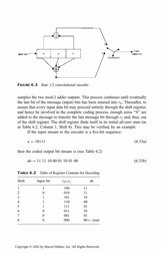
samples the two mod-2 adder outputs. This process continues until eventually
the last bit of the message (input) bits has been entered into r0. Thereafter, to
ensure that every input data bit may proceed entirely through the shift register,
and hence be involved in the complete coding process, enough zeros ‘‘0’’ are
added to the message to transfer the last message bit through r2 and, thus, out
of the shift register. The shift register finds itself in its initial all-zero state (as
in Table 6.2, Column 1, Shift 8). This may be verified, by an example.
If the input stream to the encoder is a five-bit sequence:
x ¼ 10111 ð6:33aÞ
then the coded output bit stream is (see Table 6.2)
ab ¼ 11 11 10 00 01 10 01 00 ð6:33bÞ
FIGURE 6.3 Rate 1/2 convolutional encoder.
TABLE 6.2 Table of Register Contents for Decoding
Shift Input bit r0r1r2 ab
1 1 100 11
2 0 010 11
3 1 101 10
4 1 110 00
5 1 111 01
6 0 011 10
7 0 001 01
8 0 000 00 reset
Copyright © 2002 by Marcel Dekker, Inc. All Rights Reserved.
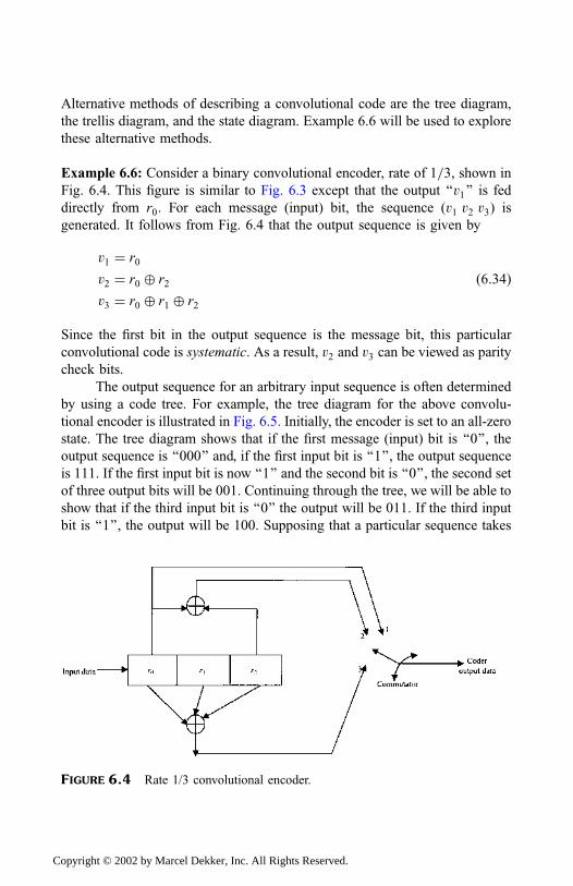
Alternative methods of describing a convolutional code are the tree diagram,
the trellis diagram, and the state diagram. Example 6.6 will be used to explore
these alternative methods.
Example 6.6: Consider a binary convolutional encoder, rate of 1=3, shown in
Fig. 6.4. This figure is similar to Fig. 6.3 except that the output ‘‘v1’’ is fed
directly from r0. For each message (input) bit, the sequence (v1 v2 v3) is
generated. It follows from Fig. 6.4 that the output sequence is given by
v1 ¼ r0
v2 ¼ r0 � r2
v3 ¼ r0 � r1 � r2
ð6:34Þ
Since the first bit in the output sequence is the message bit, this particular
convolutional code is systematic. As a result, v2 and v3 can be viewed as parity
check bits.
The output sequence for an arbitrary input sequence is often determined
by using a code tree. For example, the tree diagram for the above convolu-
tional encoder is illustrated in Fig. 6.5. Initially, the encoder is set to an all-zero
state. The tree diagram shows that if the first message (input) bit is ‘‘0’’, the
output sequence is ‘‘000’’ and, if the first input bit is ‘‘1’’, the output sequence
is 111. If the first input bit is now ‘‘1’’ and the second bit is ‘‘0’’, the second set
of three output bits will be 001. Continuing through the tree, we will be able to
show that if the third input bit is ‘‘0’’ the output will be 011. If the third input
bit is ‘‘1’’, the output will be 100. Supposing that a particular sequence takes
FIGURE 6.4 Rate 1/3 convolutional encoder.
Copyright © 2002 by Marcel Dekker, Inc. All Rights Reserved.
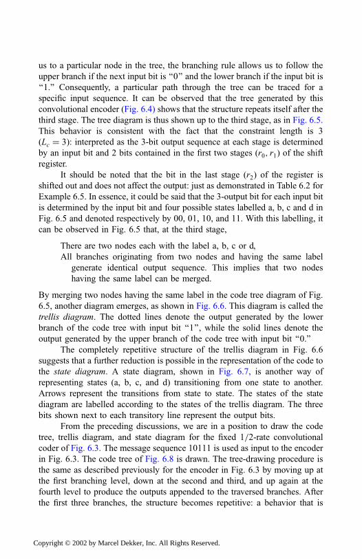
us to a particular node in the tree, the branching rule allows us to follow the
upper branch if the next input bit is ‘‘0’’ and the lower branch if the input bit is
‘‘1.’’ Consequently, a particular path through the tree can be traced for a
specific input sequence. It can be observed that the tree generated by this
convolutional encoder (Fig. 6.4) shows that the structure repeats itself after the
third stage. The tree diagram is thus shown up to the third stage, as in Fig. 6.5.
This behavior is consistent with the fact that the constraint length is 3
(Lc ¼ 3): interpreted as the 3-bit output sequence at each stage is determined
by an input bit and 2 bits contained in the first two stages (r0; r1) of the shift
register.
It should be noted that the bit in the last stage (r2) of the register is
shifted out and does not affect the output: just as demonstrated in Table 6.2 for
Example 6.5. In essence, it could be said that the 3-output bit for each input bit
is determined by the input bit and four possible states labelled a, b, c and d in
Fig. 6.5 and denoted respectively by 00, 01, 10, and 11. With this labelling, it
can be observed in Fig. 6.5 that, at the third stage,
There are two nodes each with the label a, b, c or d,
All branches originating from two nodes and having the same label
generate identical output sequence. This implies that two nodes
having the same label can be merged.
By merging two nodes having the same label in the code tree diagram of Fig.
6.5, another diagram emerges, as shown in Fig. 6.6. This diagram is called the
trellis diagram. The dotted lines denote the output generated by the lower
branch of the code tree with input bit ‘‘1’’, while the solid lines denote the
output generated by the upper branch of the code tree with input bit ‘‘0.’’
The completely repetitive structure of the trellis diagram in Fig. 6.6
suggests that a further reduction is possible in the representation of the code to
the state diagram. A state diagram, shown in Fig. 6.7, is another way of
representing states (a, b, c, and d) transitioning from one state to another.
Arrows represent the transitions from state to state. The states of the state
diagram are labelled according to the states of the trellis diagram. The three
bits shown next to each transitory line represent the output bits.
From the preceding discussions, we are in a position to draw the code
tree, trellis diagram, and state diagram for the fixed 1=2-rate convolutional
coder of Fig. 6.3. The message sequence 10111 is used as input to the encoder
in Fig. 6.3. The code tree of Fig. 6.8 is drawn. The tree-drawing procedure is
the same as described previously for the encoder in Fig. 6.3 by moving up at
the first branching level, down at the second and third, and up again at the
fourth level to produce the outputs appended to the traversed branches. After
the first three branches, the structure becomes repetitive: a behavior that is
Copyright © 2002 by Marcel Dekker, Inc. All Rights Reserved.
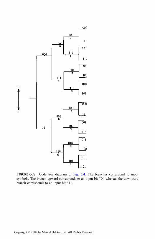
FIGURE 6.5 Code tree diagram of Fig. 6.4. The branches correspond to input
symbols. The branch upward corresponds to an input bit ‘‘0’’ whereas the downward
branch corresponds to an input bit ‘‘1’’.
Copyright © 2002 by Marcel Dekker, Inc. All Rights Reserved.
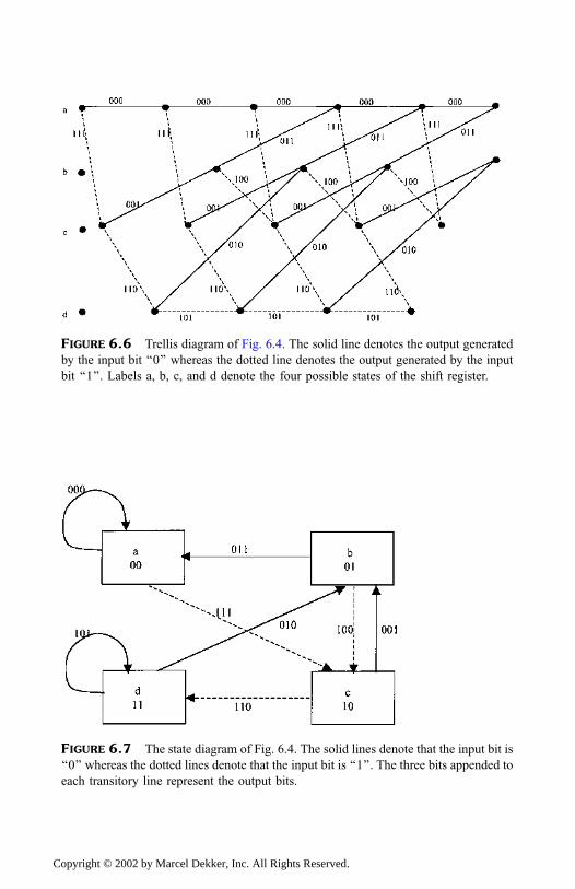
FIGURE 6.6 Trellis diagram of Fig. 6.4. The solid line denotes the output generated
by the input bit ‘‘0’’ whereas the dotted line denotes the output generated by the input
bit ‘‘1’’. Labels a, b, c, and d denote the four possible states of the shift register.
FIGURE 6.7 The state diagram of Fig. 6.4. The solid lines denote that the input bit is
‘‘0’’ whereas the dotted lines denote that the input bit is ‘‘1’’. The three bits appended to
each transitory line represent the output bits.
Copyright © 2002 by Marcel Dekker, Inc. All Rights Reserved.
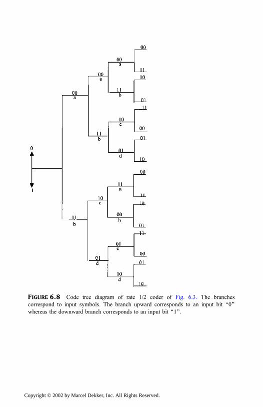
FIGURE 6.8 Code tree diagram of rate 1/2 coder of Fig. 6.3. The branches
correspond to input symbols. The branch upward corresponds to an input bit ‘‘0’’
whereas the downward branch corresponds to an input bit ‘‘1’’.
Copyright © 2002 by Marcel Dekker, Inc. All Rights Reserved.
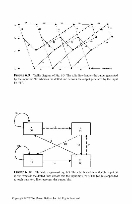
FIGURE 6.9 Trellis diagram of Fig. 6.3. The solid line denotes the output generated
by the input bit ‘‘0’’ whereas the dotted line denotes the output generated by the input
bit ‘‘1’’.
FIGURE 6.10 The state diagram of Fig. 6.3. The solid lines denote that the input bit
is ‘‘0’’ whereas the dotted lines denote that the input bit is ‘‘1’’. The two bits appended
to each transitory line represent the output bits.
Copyright © 2002 by Marcel Dekker, Inc. All Rights Reserved.
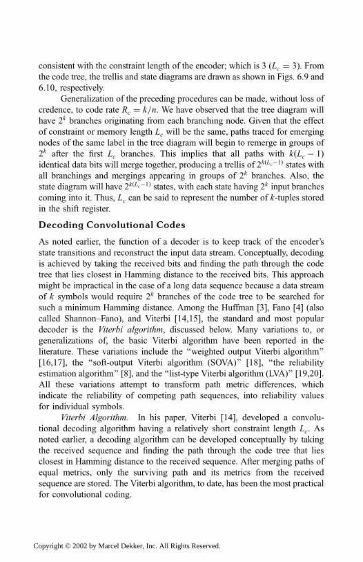
consistent with the constraint length of the encoder; which is 3 (Lc ¼ 3). From
the code tree, the trellis and state diagrams are drawn as shown in Figs. 6.9 and
6.10, respectively.
Generalization of the preceding procedures can be made, without loss of
credence, to code rate Rc ¼ k=n. We have observed that the tree diagram will
have 2k branches originating from each branching node. Given that the effect
of constraint or memory length Lc will be the same, paths traced for emerging
nodes of the same label in the tree diagram will begin to remerge in groups of
2k after the first Lc branches. This implies that all paths with kðLc � 1Þidentical data bits will merge together, producing a trellis of 2kðLc�1Þ states withall branchings and mergings appearing in groups of 2k branches. Also, the
state diagram will have 2kðLc�1Þ states, with each state having 2k input branchescoming into it. Thus, Lc can be said to represent the number of k-tuples stored
in the shift register.
Decoding Convolutional Codes
As noted earlier, the function of a decoder is to keep track of the encoder’s
state transitions and reconstruct the input data stream. Conceptually, decoding
is achieved by taking the received bits and finding the path through the code
tree that lies closest in Hamming distance to the received bits. This approach
might be impractical in the case of a long data sequence because a data stream
of k symbols would require 2k branches of the code tree to be searched for
such a minimum Hamming distance. Among the Huffman [3], Fano [4] (also
called Shannon–Fano), and Viterbi [14,15], the standard and most popular
decoder is the Viterbi algorithm, discussed below. Many variations to, or
generalizations of, the basic Viterbi algorithm have been reported in the
literature. These variations include the ‘‘weighted output Viterbi algorithm’’
[16,17], the ‘‘soft-output Viterbi algorithm (SOVA)’’ [18], ‘‘the reliability
estimation algorithm’’ [8], and the ‘‘list-type Viterbi algorithm (LVA)’’ [19,20].
All these variations attempt to transform path metric differences, which
indicate the reliability of competing path sequences, into reliability values
for individual symbols.
Viterbi Algorithm. In his paper, Viterbi [14], developed a convolu-
tional decoding algorithm having a relatively short constraint length Lc. As
noted earlier, a decoding algorithm can be developed conceptually by taking
the received sequence and finding the path through the code tree that lies
closest in Hamming distance to the received sequence. After merging paths of
equal metrics, only the surviving path and its metrics from the received
sequence are stored. The Viterbi algorithm, to date, has been the most practical
for convolutional coding.
Copyright © 2002 by Marcel Dekker, Inc. All Rights Reserved.
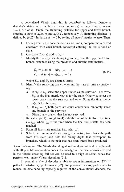
A generalized Viterbi algorithm is described as follows. Denote a
decoder’s states as s, with its metric as mðs; tÞ at any time t, where
s ¼ a; b; c or d. Denote the Hamming distance for upper and lower branch
entering a state as dU ðs; tÞ and dLðs; tÞ, respectively. A Hamming distance is
defined by (6.22). Initialize at t ¼ 0 by setting all states’ metrics to zero. Then:
1. For a given trellis node or state s and time t, compare the received
codeword with each branch codeword entering the trellis node or
state.
2. Calculate dU ðs; tÞ and dLðs; tÞ.3. Modify the path by calculating DU and DL from the upper and lower
branch distances using the previous and current state metrics:
Du ¼ dU ðs; tÞ þ mðst�1; t � 1ÞDl ¼ dLðs; tÞ þ mðst�1; t � 1Þ ð6:35Þ
where DU and DL are abstract terms.
4. Identify the surviving branch entering the state at time t consider-
ing:
a. If DU < DL select the upper branch as the survivor. Then write
DU as the final metric mðs; tÞ for the state. Otherwise select thelower branch as the survivor and write DL as the final metric
mðs; tÞ for the state,
b. If DU ¼ DL both paths are equal contenders; randomly select
any branch as the survivor.
c. Discard any branch that has not survived.
5. Repeat steps (1) through to (4) until the end of the trellis tree at time
t ¼ trec, where trec is the time when the final trellis state has been
reached.
6. Form all final state metrics, i.e., mðs; trecÞ.7. Select the minimum distance (dmin) or metric, trace back the path
from this state, and note the binary digits that correspond to
branches, which is the path that has been traced back produced.
Aword of caution! The Viterbi decoding algorithm does not work equally well
with all possible convolution codes. Knowledge of the mechanisms involved
in the Viterbi decoding failures can be used to design or select codes that
perform well under Viterbi decoding [21].
In general, a Viterbi decoder is able to retain information on 2kðLc�1Þ
paths for satisfactory performance [22]. For practical reasons, particularly to
reduce the data-handling capacity required of the convolutional decoder, the
Copyright © 2002 by Marcel Dekker, Inc. All Rights Reserved.
trellis depth is approximated to 5Lc nodes. This allows decoding of only the
oldest received sequence within the trellis and selecting the path with the
fewest errors, while deleting the remaining paths.
6.3 SUMMARY
The transmission of data over a communication link is highly likely to result in
some errors occurring in the received data, for at least a small proportion of
time, because of noise added by the transmission medium and system. Some
techniques on how the errors can be detected and correction effected have
been explored in this chapter. These techniques are forward error correcting,
broadly classified under two headings: block codes and convolutional codes.
In the block coding techniques, the encoder splits up incoming data
stream into blocks of finite-number digits and processes each block by adding
extra bits (called redundancy) according to a predefined algorithm. The output
of the encoder is a codeword with another finite number of digits. A few
subsets of linear block codes, such as Hamming, cyclic, and BCH, have also
been discussed. Their importance is the existence of practical decoding
techniques.
In the convolutional coding techniques, the encoder processes the
incoming data stream continuously while its decoder employs the Viterbi
algorithm among others. Convolutional codes are very popular because they
are simple in concept and in practice to utilize.
Examples were sparingly used as illustrative tools to explain these
forward error correction techniques.
BIBLIOGRAPHY
1. Berlekamp, E.R. (1968). Algebraic Coding Theory. McGraw-Hill: New York.
2. Hagenauer, J. and Hoeher, P. (1989). AViterbi algorithm with soft-decision outputs
and its applications, GLOBECOM’89 Dallas, Texas Conference Proc., 1680–
1686.
REFERENCES
1. Feher, K. (1984) Digital Communications: Satellite=Earth Station Engineering.
Prentice-Hall.
2. Shannon, C.E. (1948). A mathematical theory of communication, Bell System Tech
J., vol. 26.
Copyright © 2002 by Marcel Dekker, Inc. All Rights Reserved.
3. Huffman, D.A. (1952). A method for the construction of minimum redundancy
codes, Proc. IRE, 40, 1098–1101.
4. Fano, R.M. (1963). A heuristic discussion of probabilistic decoding, IEEE Trans.
Information Theory, 9, 64–74.
5. Okunev, I.B. (1997). Phase and Phase-Difference Modulation in Digital Commu-
nications. Artech House.
6. Lee, E.A. and Messerschmitt, D.G. (1994). Digital Communication. Kluwer
Academic.
7. Lin, S. (1970). An Introduction to Error Correcting Codes. Prentice-Hall.
8. Huber, J. and Rueppel, A. (1990). Reliability estimation for symbols detected by
Trellis decoders (in German), AEU, 44, 8–21.
9. Lin, S. and Costello, D.J. (1983). Error Control Coding: Fundamentals and
Applications. Prentice-Hall.
10. Shamnugam, K.S. (1979). Digital and Analog Communication Systems. John
Wiley.
11. Peterson, W.W. (1972). Error Correcting Codes. MIT Press.
12. Bose, R.C and Ray-Chaudhuri, D.K. (1960). On a class of error correcting binary
group codes, Information Control, 3, 68–79.
13. Pratt, T. and Bostian, C.W. (1986). Satellite Communications. John Wiley.
14. Viterbi, A.J. (1967). Error bounds for convolutional codes and an asymptotically
optimum decoding algorithm, IEEE Trans. Information Theory, 13, 260–269.
15. Viterbi, A.J. and Omura, J.K. (1979). Principles of Digital Communication and
Coding. McGraw-Hill.
16. Battail, G. (1989). Building long codes by combination of simple ones, thanks to
weighted-output decoding, Proc. URSI ISSSE, Erlangen, 634–637.
17. Berrou, C. and Glavieux, A. (1996). Near optimum error correcting coding and
decoding, IEEE Trans. Communications, 44:10, 1261–1271.
18. Proakis, J.G. (1995). Digital Communications. McGraw-Hill.
19. Hashimoto, T. (1987). A list-type reduced-constraint generalization of the Viterbi
algorithm, IEEE Trans. Information Theory, 26, 540–547.
20. Sundberg, C.W. (1992). Generalizations of the Viterbi algorithm with applications
in radio systems in Advanced Methods for Satellite and Deep Space Communica-
tions. Springer-Verlag.
21. Rorabaugh, C.B. (1996). Error Coding Cookbook; Practical C=Cþþ Routines
and Recipes for Error Detection and Correction. McGraw-Hill.
22. Heller, J.A. and Jacobs, I.M. (1981). Viterbi decoding for satellite and space
communications, IEEE Trans. Communications, 19, 835–848.
PROBLEMS
1. A channel-coded CDMA system uses a rate 1=2, 7-stage convolutional
encoder before addressing at each transmitter. Determine by which factor
Copyright © 2002 by Marcel Dekker, Inc. All Rights Reserved.
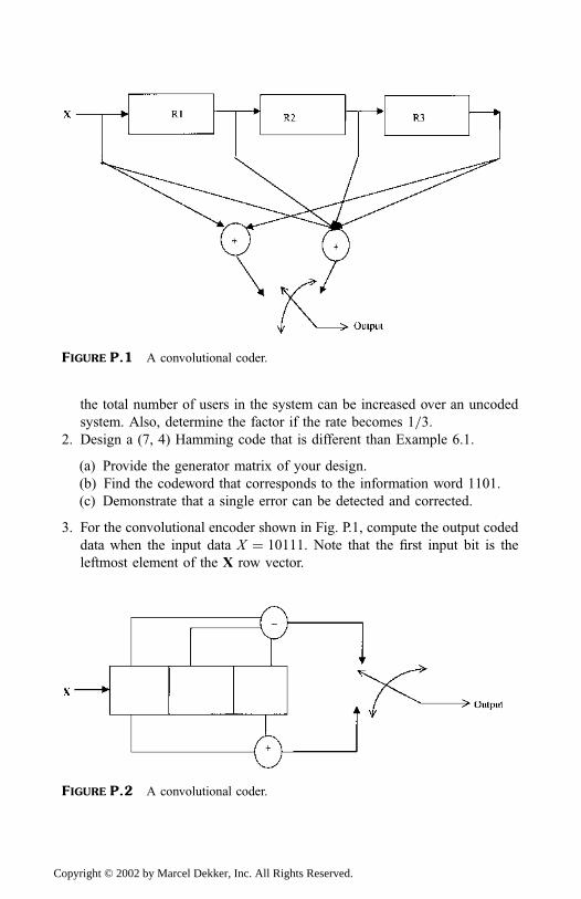
the total number of users in the system can be increased over an uncoded
system. Also, determine the factor if the rate becomes 1=3.2. Design a (7, 4) Hamming code that is different than Example 6.1.
(a) Provide the generator matrix of your design.
(b) Find the codeword that corresponds to the information word 1101.
(c) Demonstrate that a single error can be detected and corrected.
3. For the convolutional encoder shown in Fig. P.1, compute the output coded
data when the input data X ¼ 10111. Note that the first input bit is the
leftmost element of the X row vector.
FIGURE P.1 A convolutional coder.
FIGURE P.2 A convolutional coder.
Copyright © 2002 by Marcel Dekker, Inc. All Rights Reserved.

4. Draw a block diagram for a convolutional coder that has a rate of 2=3 and a
constraint length of 5.
5. A convolutional coder is shown in Fig. P.2.
(a) Determine the code rate and constraint length.
(b) Draw the state diagram and code trellis.
(c) Draw the Viterbi trellis.
(d) For the received codeword X ¼ 11 10 11 11 01 01, trace the path
sequence.
Copyright © 2002 by Marcel Dekker, Inc. All Rights Reserved.
7
Regulatory Agencies andProcedures
The regulation that covers satellite communication networks occurs on three
levels: international, regional, and national. The interaction among the three
regulatory levels is briefly discussed in this chapter.
7.1 INTERNATIONAL REGULATIONS
The reader might query the purpose and need for international regulations.
This emerges as the international community realizes that the radiofrequency
spectrum and the geostationary satellite orbit are two finite natural resources
available to humans. Each of these resources has the unique property of being
conserved if it is used properly and wasted if it is not used properly. To
conserve the precious commodity, certain requirements need to be fulfilled.
Copyright © 2002 by Marcel Dekker, Inc. All Rights Reserved.
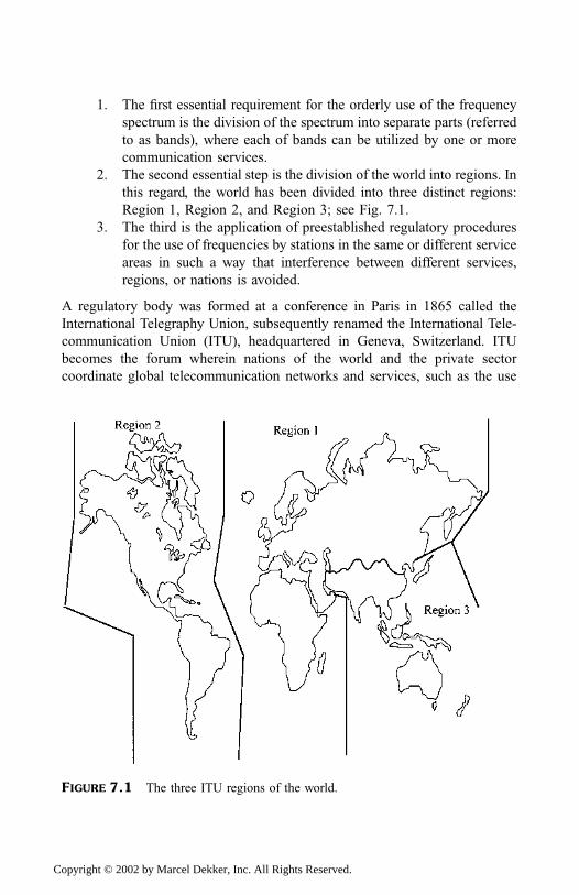
1. The first essential requirement for the orderly use of the frequency
spectrum is the division of the spectrum into separate parts (referred
to as bands), where each of bands can be utilized by one or more
communication services.
2. The second essential step is the division of the world into regions. In
this regard, the world has been divided into three distinct regions:
Region 1, Region 2, and Region 3; see Fig. 7.1.
3. The third is the application of preestablished regulatory procedures
for the use of frequencies by stations in the same or different service
areas in such a way that interference between different services,
regions, or nations is avoided.
A regulatory body was formed at a conference in Paris in 1865 called the
International Telegraphy Union, subsequently renamed the International Tele-
communication Union (ITU), headquartered in Geneva, Switzerland. ITU
becomes the forum wherein nations of the world and the private sector
coordinate global telecommunication networks and services, such as the use
FIGURE 7.1 The three ITU regions of the world.
Copyright © 2002 by Marcel Dekker, Inc. All Rights Reserved.
of the radiofrequency spectrum, and set standards regarding interference
levels, equipment characteristics, and communication protocols for all tele-
communications systems. This forum also establishes procedures for the
coordination of frequency spectrum use by member states [1].
With the advent of space technology, new provisions have been adopted
in the Radio regulations. These are required to regulate the use of space
radiocommunications, particularly the geostationary and nongeostationary
orbits.
It should be emphasized that the underlying principle upon which the
effectiveness of rules and regulations is based is the voluntary undertaking by
each signatory to comply and ensure international cooperation. Though ITU
does not have the authority to enforce its rules and regulations, nations have
generally adhered to its recommendations as a matter of policy.
To fulfill its mission, ITU established an administrative body, which
consists of permanent organizations that convene regional and world confer-
ences to discuss and establish policy to guide its permanent organ and member
nations’ telecommunication services. The administrative body includes
I. The General Secretariat
II. Administrative Council
III. The International Frequency Registration Board (IFRB)
IV. The International Radio Consultative Committee (CCIR)
V. The International Telegraph and Telephone Consultative Council
(CCITT)
The General Secretariat has an elected Secretary General and Deputy. The
secretariat, being the collective name for the permanent organizations asso-
ciated with ITU, is charged with discharging the administrative duties of the
ITU but has no authority to establish basic policy. The plenary assembly is the
main functioning body of the ITU. It usually meets every four years, where
draft Reports and Recommendations prepared by study groups within the
permanent organs (e.g., CCIR) are considered and approved. It is during these
plenary sessions that the Secretary General, its Deputy, and the administrative
board members are elected. The Plenary assembly also elects the directors of
the CCITT and CCIR.
It should be noted that many of the approved Reports and Recommen-
dations form the basis for revision of the Radio regulations of the world
administrative conferences. Administrative conferences are normally convened
to consider specific telecommunication matters: can be regional or world
conferences. Radio Regulations define the rules to be applied in using the
spectrum and the orbit, as well as the rights and obligations resulting from this
Copyright © 2002 by Marcel Dekker, Inc. All Rights Reserved.
use. The ITU Radio Regulations govern satellite communication networks.
The approved Reports and Recommendations are not of themselves obligatory
in the same content as the Radio Regulations, but serve as standards for use by
the world’s telecommunication community. World administrative radio confer-
ences (WARCs) elect the five members of the International Frequency
Registration Board (IFRB). WARCs may also adopt resolutions and
recommendations. Only member states vote at these conferences, but repre-
sentatives of other international organizations and private sectors can attend
the sessions.
The International Radio Consultative Committee (CCIR) and the Inter-
national Telegraph and Telephone Consultative Council (CCITT) convene
study groups in order to recommend technical specifications for equipment
and to conduct propagation, interference, and other types of analyses. The
work of these committees (CCIR and CCITT) has considerable influence on
system planners, network designers, and equipment manufacturers, and to a
lesser degree on operators. For this reason the next subsections briefly describe
their origin, responsibilities, and functions.
7.1.1 CCIR
The CCIR duties are (as defined under the International Telecommunication
Convention, Nairobi, 1982, first part, chapter 1, Article II, No. 83) to study
technical and operating questions relating specifically to radiocommunication
without limit of frequency range, and to issue recommendations on them. The
objectives of the CCIR are in particular:
1. To provide the technical bases for use by the administrative radio
conferences and radiocommunication services for efficient utiliza-
tion of the radiofrequency spectrum and the geostationary satellite
orbit, bearing in mind the needs of the various radio services
2. To recommend performance standards for radio systems and tech-
nical arrangements, which ensure their effective and compatible
interworking in international telecommunications
3. To collect, exchange, analyze, and disseminate technical informa-
tion resulting from the studies by the CCIR, and other information
available, for the development, planning and operation of radio
systems, including any necessary special measures required to
facilitate the use of such information in developing countries
Copyright © 2002 by Marcel Dekker, Inc. All Rights Reserved.
The CCIR works through the medium of a number of study groups, each
dealing with a particular aspect of radio communication. The CCIR has eleven
study groups:
1. Spectrum utilization and monitoring
2. Space research and radio astronomy
3. Fixed service at frequencies below about 30MHz
4. Fixed satellite service
5. Propagation in nonionized medium
6. Ionospheric propagation
7. Standard frequencies and time signals
8. Mobile services
9. Fixed service using radio relay systems
10. Broadcasting service—sound
11. Broadcasting service—television
The members of these study groups come primarily from the nations most
technically advanced in the telecommunication field: these include the United
States, Russia, the United Kingdom, Canada, France, Japan, Australia, etc.
Since the reports and recommendations of these study groups are nonbinding,
an effort is made to achieve consensus and unanimity in their findings.
Naturally, national interests of the member nations are jealously ‘‘guarded,
awaiting’’ in the preparation of the consensus documents.
The most relevant of these groups to satellite communication networks
is Study Group 4, which deals with fixed services using satellites. A lot of
interactions occur between study groups 4 and 9, in defining the criteria for
assessing interference between satellite networks and terrestrial terminals in
shared bands.
7.1.2 CCITT
The CCITT was formed in 1956 as a result of the merger of two ITU
organizations, the CCIT (the technical consultative committee for telephone)
and the CCIF (technical consultative committee for telegraphy). The primary
function of the CCITT is to standardize, promote, and ensure the operation of
international telecommunication systems. This goal is accomplished by
establishing recommended standards for performance, interconnection, and
maintenance of international networks for telephone, telegraph, and data
communications.
Copyright © 2002 by Marcel Dekker, Inc. All Rights Reserved.
Within the CCITT structure exist a number of study groups that provide
the work classification or specialization for developing the recommendations.
The CCITT has 17 study groups:
I. Definition and operational aspects of telegraph and user
services (telex, facsimile, videotex, etc.)
II. Telephone operation and quality of service
III. General tariff principles
IV. Transmission maintenance of international lines, circuits, and
chains of circuits; maintenance of automatic and semiautomatic
networks
V. Protection against dangers and disturbances of electromagnetic
origin
VI. Protection and specifications of cable sheaths and poles
VII. Data communication networks
VIII. Terminal equipment for services (telex, facsimile, videotex,
etc.)
IX. Telegraph networks and terminal equipment
X. Telegraph switching
XI. Telephone switching and signalling
XII. Telephone transmission performance and local telephone
networks
XIV. This group has similar function as Group 8
XV. Transmission system
XVI. Telephone circuits
XVII. Data transmission over the telephone network
XVIII. Digital networks
There are joint CCIR and CCITT study groups, namely the CMV and CMTT,
responsible for vocabulary and transmission of sound broadcasting and
television signals over long distances, respectively.
The recommendations of Group XVIII in particular have paved the
way for the standardization of interfaces for public data networks and
protocols for international packet-switched data networks. Their work, with
some contributions from Groups I, II, and XVII, has provided significant
building blocks for integrated services digital networks (ISDN) and in turn
integrated services digital satellite networks (ISDSN). With our rapidly
changing technology, particularly in multimedia and digital baseband proces-
sing, Group 4 of CCIR has become involved in order to standardize ISDSN
services.
Copyright © 2002 by Marcel Dekker, Inc. All Rights Reserved.
7.1.3 IFRB
The International Frequency Registration Board (IFRB) is a collegiate body
that possesses through its members a thorough knowledge of radiocommuni-
cations and the problems of their use in various regions throughout the world.
The board members are supposed to be custodians of an international public
trust. Its composition and duties are defined in Articles 10 and 57 of the
Plenipotentiary Conference of 1947. Although IFRB’s composition, duties,
and working methods have undergone some changes since then, its essential
duties can be summarized as follows:
I. To effect an orderly recording of frequency assignments made by
different countries
II. To effect an orderly recording of the orbital positions assigned by
countries to geostationary satellites
III. To advise countries on efficient utilization of the spectrum and
geostationary satellite orbit
IV. To follow the procedures laid down in the Radio Regulations or by
Administrative Conferences
V. To provide technical assistance in organizing and preparing for
radio conferences in consultation with other permanent organs of
ITU, and to assist developing countries in their preparations for
such conferences
VI. To maintain the records essential for the performance of its
duties
The Board’s duty is to examine all frequency assignment notices submitted to
it by administrations, and formulate in respect of each notice what the Radio
Regulations term a finding. Each finding is a statement of a juridical nature
based on regulatory and technical grounds. It results in a decision either to
record an assignment in the Master International Frequency Register (MIRF)
in accordance with the Radio Regulations or to return the notice to the
notifying administration because of its nonconformity with one or more
relevant provisions. Once the assignment is entered in the MIRF, it has
international recognition and certain legitimacy. The procedures governing
notification and registration of frequency assignments in the MIRF may be
broadly subdivided into the areas of coordination, notification, examination,
and registration.
Copyright © 2002 by Marcel Dekker, Inc. All Rights Reserved.
7.2 NATIONAL AND REGIONAL REGULATIONS
It is logical to institute a national or regional regulatory body that oversees and
manages the country’s or region’s spectrum and adopt national (or regional)
legislation that includes, as the basic minimum, the essential provisions of the
International Telecommunication Convention. This is necessary because the
International Telecommunication Convention and Radio Regulations annexed
to the Convention are intergovernmental treaties, which have been ratified and
accepted by the governments of the countries. These governments are bound to
apply the provisions of the treaties in their countries and the other geographical
areas under their jurisdiction. In reality, a regional body is formed in the
context of bilateral agreements with neighboring countries to settle policy or
operational issues, for the purpose of coordinating the establishment of
telecommunication systems and importantly for other items of mutual interest.
To this effect, a country must adopt national legislation, that is enforce-
able, enabling the national regulatory body
1. To develop regulations for effective use of spectrum on the basis of
national or regional priorities.
2. To coordinate and oversee long-term spectrum management policy
and planning.
3. To identify the spectrum requirements, which satisfy the need of the
country or region.
4. To develop technical standards.
5. To monitor, detect, and resolve operational irregularities, harmful
interference, and technical ambiguities.
6. To conduct negotiations relating to frequency spectrum manage-
ment and related matters that may improve technical and adminis-
trative cooperation with other countries and international
organizations.
7. To keep accurate and up-to-date data records. This is a requirement
of utmost importance for effective national, regional, and interna-
tional coordination; licensing and enforcement activities; policy
formulation; interference investigation and resolution; and financial
considerations.
8. To participate in ITU Study Group(s) where national or regional
interests are safeguarded.
9. To provide personnel training for frequency management, such as
training in the IFRB, CCIR, and that supplemented by other means
like seminars organized by the IFRB, exchange of staff with other
countries, and hands-on operational experience on the job.
Copyright © 2002 by Marcel Dekker, Inc. All Rights Reserved.

The national or regional spectrum management body should therefore admin-
ister day-to-day spectrum applications originating from the public and govern-
mental sectors. In some instances, the flow of activities concerned with the
approval, licensing, spectrum allocation, and international coordination of
commercial and military satellite systems may be handled by different sections
of the national or regional body according to the requirements and resources of
the country concerned.
7.3 SUMMARY
The regulation that covers satellite networks occurs on three levels: interna-
tional, regional, and national. The underlying principle on which the effec-
tiveness of the international and regional regulations is based is the voluntary
undertaking by the governments that signed the regulations to comply with
them and ensure international and regional cooperation. The regulatory bodies
formed by these governments have the legislative power, within their jurisdic-
tion, to ensure and enforce an orderly distribution of frequency spectrum in
compliance with the treaties acceded to and ensuring no interference in the
spectrum assigned to the operator(s). The underlying principle and the
interaction among the three regulatory levels have been discussed in this
chapter.
REFERENCE
1. ITU (1988). Booklet on national frequency management. Geneva.
PROBLEM
Study the radio communication regulatory agency of your country. Is there any
way you can rationalize the various departments within the agency?
Copyright © 2002 by Marcel Dekker, Inc. All Rights Reserved.
8
Mobile Satellite System Services
8.1 OVERVIEW
Until the introduction of international maritime satellite communications
systems (INMARSAT) to serve ships at sea, all satellite communication
links were between fixed locations. The introduction of maritime services
served to focus attention on the whole field of mobile communications and
opened up a range of novel opportunities. These include
1. Standardization of system solutions; the most successful standar-
dized systems is the Global System for Mobile Communications
(GSM). The GSM architecture is based on terrestrial switched
network.
2. Provision of personalized services and mobility as well as inter-
active telecommunications systems (e.g., short text messaging)
using small handheld terminals and the need for a single telephone
number worldwide for a roaming traveller.
Copyright © 2002 by Marcel Dekker, Inc. All Rights Reserved.
3. The need to expand or enhance the capability of the existing
terrestrial and cellular communication networks to sparsely popu-
lated regions, remote areas, or areas where a communication
infrastructure is suddenly destroyed or has never existed.
4. Provision of very accurate navigational data, ship-to-shore search
and rescue messages in emergencies.
5. Direct broadcast television, instant broadcast of impending danger,
and specialized business services.
6. Systems tracking for logistic reasons.
This chapter examines the basic structure of a mobile satellite system (MSS)
and its interaction with land-based public-switched digital networks, in
particular the integrated service digital network (ISDN). Since the services
covered by ISDN are also, in principle, provided by a mobile satellite system
network, it is considered necessary to discuss in some detail the basic
architecture of ISDN as well as its principal functional groups in terms of
reference configurations, applications, and protocol. The chapter finishes by
briefly examining the cellular mobile system including cell assignment and the
internetworking principle as well as technological shortcomings to providing
efficient Internet access over satellite links.
8.2 MOBILE SATELLITE SYSTEMSARCHITECTURE
A mobile satellite system (MSS) is a system that provides radio communica-
tion services between
1. Mobile earth stations and one or more satellite stations
2. Mobile earth stations by means of one or more satellites
3. Satellites.
Figure 8.1 shows the basic architecture of a mobile satellite system (MSS)
with a land-based digital switched network (LDSN) and intersatellite cross
link. Assuming that a new-generation mobile satellite is being designed for
Fig. 8.1, the total spacecraft system such as power, guidance and control, and
data handling would have advanced-technology components. The satellite
would contain onboard digital signal processors (DSP) and memory for
onboard data processing capability, and onboard fast packet switches. The
onboard fast packet switches would be capable of supporting space-optimized
traffic from multiple earth stations.
Copyright © 2002 by Marcel Dekker, Inc. All Rights Reserved.
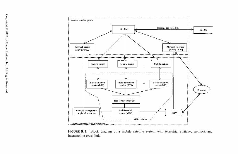
FIGURE 8.1 Block diagram of a mobile satellite system with terrestrial switched network and
intersatellite cross link.
Copyright ©
2002 by Marcel D
ekker, Inc. All R
ights Reserved.
The DSP will be responsible for resource management and control
including encryption=decryption, channelization, demodulation, and deco-
ding=encoding. This functionality has been discussed in the previous chapters.
As stated earlier, since most, if not all, of the services covered by the MSS are,
in principle, provided by terrestrial switched digital networks (e.g. ISDN) we
will attempt to explain some the concepts applicable to ISDN that have not
been previously dealt with in previous chapters.
The network routers (gateways) allow
Seamless intersatellite cross link; that is, direct data transfers from one
satellite to another,
Seamless connectivity for users anywhere in the world through mobile=fixed earth stations and public-switched digital networks
Traffic shaping, resource accounting, cache for traffic redirection and
load sharing, and integrated network management to support a
myriad of simultaneous connections per satellite
Any mobile station registered on the mobile satellite network is interconnected
to any available channel of the network interface gateway (NIG) through
proper channel assignments issued by the network access gateway (NAG).
When the satellite illuminates a particular area or region, the mobile
satellite system routes intended messages (e.g., telephone calls, data, etc.)
through the ground networks (e.g., ISDN), ground stations, or directly to the
user terminals. User terminals can be personal terminals for individual
subscribers or multiuser terminals for corporate (e.g., Internet providers,
communication resellers, etc) and communal residential subscribers.
The public terrestrial switched networks, called in this text Land-based
Digital Switched Network (LDSN), contain the integrated services digital
network (ISDN) and mobile communications systems to provide end users
with efficient communication services between fixed and fixed terminals, fixed
and mobile terminals, and mobile and mobile terminals. In the network
arrangement shown in Fig. 8.1, any mobile stations using the services of
PLSN can communicate both signalling and bearer traffic to the base
transceiver station (BTS) that provides the most favorable radiofrequency
(RF) signal. This establishes an association between the mobile station’s
geographic location and the closest BTS. As the mobile station moves from
the coverage area of one BTS to another, the first association is released and a
new one is formed. This procedure is called handover. The base station
controller (BSC) and mobile switching center (MSC) manage radio resources,
channel assignments, and handover services. A single BSC can control
multiple BTSs. A single MSC can control multiple BSCs. Multiple MSCs
Copyright © 2002 by Marcel Dekker, Inc. All Rights Reserved.
may reside within a single LDSN. The network management application
process (MAP) defines services for signalling among several MSCs. In
principle, all the services MAP defines and provides are applicable to the
MSS. This duality of services becomes obvious when considering MAP in
Sec. 8.2.1 since the services are offspring of the parent class of LDSN.
As previously discussed in Chap. 5, sufficient access can be provided by
satellites; however, the type and number of accesses provided depend on the
access scheme employed. As noted in Chap. 2, satellite-based transmitter and
receiver chains can operate through high-gain spot beam antennas deployed in
arrays of multiple beams to cover the desired service area on earth. If an
antenna beam is focused at a fixed area, we can use a single satellite network
access gateway to manage and control all mobile stations located within the
spot beam to provide direct data link access. Multiple network interface
gateways may be deployed, in circumstances where service areas are sparsely
distributed, to provide local terrestrial interconnection between the satellite and
public terrestrial networks for efficient routing of circuit-switched bearer
services and teleservices.
At this stage, it is considered necessary to discuss in some detail the
basic architecture of ISDN as well as its principal functional groups in terms of
reference configurations, applications, and protocol.
8.2.1 Integrated Services Digital Network (ISDN)
An integrated service digital network (ISDN) is a telecommunications network
that provides end-to-end digital connections to end users and other network
facilities. An MSS network should also, in principle, provide the services
covered by ISDN. However, network standards of MSS networks should
complement that of ISDN.
The principles of ISDN recommended by CCITT, particularly Group 18
(see Chap. 7), govern its development, protocols, and standards. Recently,
CCIR Study Group 5 (see Chap. 7) became involved with digital baseband
processing techniques, particularly for fixed and broadcasting satellite
services. As such, their work has an impact on the standardization of
integrated digital services that would be provided by satellite digital network
[1].
The next subsections discuss structural aspects of the ISDN’s commu-
nications capabilities because they [2]
1. Impose a logical structure on the communication-related aspects of
a functional group
Copyright © 2002 by Marcel Dekker, Inc. All Rights Reserved.
2. Provide a convenient framework within which we may define the
physical and logical relationship between communicating functional
groups, the types of information flows they exchange with each
other, and the protocols that govern their interaction
3. Describe the characteristics of the services that an ISDN makes
available to the end users
ISDN forms the backbone of terrestrial digital networks. To a considerable
extent, ISDN topology depends on the nature of the users and network
providers. A high-level functional representation of an ISDN is shown in
Fig. 8.2.
With this high-level functional configuration, we are able to partition the
network into a set of components that interact with each other at well-defined
interfaces. By this partition we are able to specify each component function
individually and define the relationship between the end user and those of the
network.
A number of books and papers have been devoted to this topic alone,
including those listed in the Reference section [1–6]. As a result, a brief
description of principal functional groups of ISDN is given in terms of
reference configurations; that is, abstract representations of its overall structure
into a number of functional groups.
Central to an ISDN is the interexchange network (IEN), which consists
of the physical and logic components of the backbone transmission network,
including switching facilities. These facilities comprise a number of switching
exchanges (called digital transit exchanges) and a series of transmission media
that interconnect the exchanges in a distributed network topology. The
exchanges provide the physical terminations of the interexchange transmission
media, select and allocate transmission and storage facilities for the end user
connections. Since the end users, connections can be circuit-switched or
packet-switched, both switching exchanges are normally present in an ISDN.
Packet switching is a method of transmission in which small blocks of
data called packets traverse in a store-and-forward method from source to
FIGURE 8.2 ISDN configuration.
Copyright © 2002 by Marcel Dekker, Inc. All Rights Reserved.
destination through the intermediate modes of the communications network
and in which the resources of the networks are shared among many users.
Circuit switching is a method of transferring information in which switching
and transmission functions are achieved by permanently allocating a number
of channels or bandwidth between the connections.
The common channel signalling network (CCSN) provides the physical
and transmission capacity for the transfer of connection control signals
between components of IEN. In essence, it provides the functions required
for the control, management, and maintenance of ISDN.
The subscriber-access network (SAN) consists of the part of ISDN
between the end user or subscriber and CCSN and IEN. SAN can further be
decomposed into several reference points, ensuring physical or virtual inter-
faces between the functional groups. A further decomposition of each
functional group is omitted in this text. However, an inquiring reader should
consult Helgert [2] and Ronayne [6] for a start.
The functions of each of these interconnected components (IEN, CCSN,
and SAN) do not necessarily correspond in a one-to-one manner when
specifying physical parts. The functions of each of these parts may be
contained in one or more functional groups that interact with each other
across reference points. For example, individual functions may be implemen-
ted in one or several pieces of equipment, and one piece of equipment may
perform functions in more than one group.
In order to balance the requirements of efficiency, universality, flex-
ibility, minimum complexity, and low cost on the one hand and the wide
variety of existing and evolving devices and applications on the other, three
distinct end-user-to-network interfaces have been identified, namely basic-
access, primary-access, and broadband-access, as shown in Fig. 8.3. These
three interfaces vary practically in the level of physical and logical complexity
of the functional groups, the degree of end user control over the network
connections, and the types of connections required.
In terms of data rates, the basic access operates up to 100 kbit=sec:designed primarily for single or multiple low-speed terminals, digital tele-
phones, and residential and small-business users. The data rates for the
primary access are up to 2Mbit=sec and are intended for slow-scan, high-
quality audio devices, high-speed facsimile, local area networks (LAN), and
digital private automatic branch exchange (PABX). The data rates of the
broadband-access type are in the several Gbit=sec range. The broadband-
access type of user-network interfaces is designed for video terminals, multi-
media multiplexers, high-speed file transfer, or document retrieval to name a
few.
Copyright © 2002 by Marcel Dekker, Inc. All Rights Reserved.
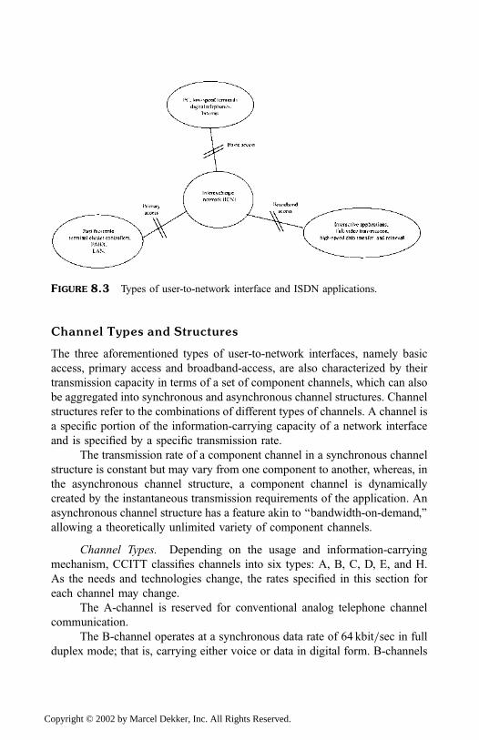
Channel Types and Structures
The three aforementioned types of user-to-network interfaces, namely basic
access, primary access and broadband-access, are also characterized by their
transmission capacity in terms of a set of component channels, which can also
be aggregated into synchronous and asynchronous channel structures. Channel
structures refer to the combinations of different types of channels. A channel is
a specific portion of the information-carrying capacity of a network interface
and is specified by a specific transmission rate.
The transmission rate of a component channel in a synchronous channel
structure is constant but may vary from one component to another, whereas, in
the asynchronous channel structure, a component channel is dynamically
created by the instantaneous transmission requirements of the application. An
asynchronous channel structure has a feature akin to ‘‘bandwidth-on-demand,’’
allowing a theoretically unlimited variety of component channels.
Channel Types. Depending on the usage and information-carrying
mechanism, CCITT classifies channels into six types: A, B, C, D, E, and H.
As the needs and technologies change, the rates specified in this section for
each channel may change.
The A-channel is reserved for conventional analog telephone channel
communication.
The B-channel operates at a synchronous data rate of 64 kbit=sec in full
duplex mode; that is, carrying either voice or data in digital form. B-channels
FIGURE 8.3 Types of user-to-network interface and ISDN applications.
Copyright © 2002 by Marcel Dekker, Inc. All Rights Reserved.
can be used at separate user-to-network interfaces to provide access to a variety
of communication modes within the ISDN. For example, two B-channels may
be attached to each other via network-provided circuit-switched or packet-
switched connections, or by permanent or temporary connections based on
circuit switching or packet switching.
The C-channel is primarily assigned to telemetry and packet-switched
data. The channel may have a variable data rate, and by virtue of its layered
protocol may be mixed with signalling information for an analog channel.
More is said about ‘‘layered protocols’’ ahead.
The D-channel primary function is to carry signalling information for
the control of circuit-switched connections involving one or more B-channels
between the end user and the network. Two types of D-channels have been
defined: layered protocols and X.25. Both operate at synchronous data rates of
either 16 kbit=sec or 64 kbit=sec in full duplex.
The E-channel is a 64 kbit=sec channel intended to transmit signalling
information for circuit-switched ISDN. It may be used for multiplexing and
providing multiple-access interfaces.
The H-channel is designed for a variety of user information functions
with channel capacity greater than the B-channel’s. Currently, there are four
types of H-channels: H0, H1, H2 and H4 with successively higher rates (see
Table 8.1.) Channels H1 and H2 exist in two versions: denoted as H11 and
H12, and H21 and H22.
The H0-channel operates at a full duplex synchronous data rate, six
times the B-channel rate, which is a submultiple of CCITT multiplex
structures (for example, 1.544Mbit=sec and 2.048Mbit=sec). TheH0-channel is suitable for standard broadcast digital audio programs.
TABLE 8.1 H-Channel Transmission (Data) Rates
Component
channel
Data rate kbit=sec Multiple of B-channel rate
H0 384 6
H1 H11 1536 24
H12 1920 30
H2 H21 32,768 512
H22 44,160 690
H4 135,168 2112
Copyright © 2002 by Marcel Dekker, Inc. All Rights Reserved.
H1-channels are designed to carry very high-speed facsimile signals,
standard compressed videoconferencing signals with reduced spatial
resolution and movement, and transmission capacity for private
network trunks.
H2-channels are intended to satisfy the requirements of fast-scan
compressed video sources.
The H4-channel is designed for a variety of user-information functions,
including enhanced video, compressed high-definition television
(HDTV) and telecasting.
For circuit-switched connections none of the H-channels carries signalling
information.
Channel Structures. Channel structures define the maximum digital
carrying capacity in terms of bit rates across the ISDN interface. The bit rates
and channel combinations are chosen to match the aggregate data rates of the
intended application(s). The fundamental objective of channel combinations is
to create the possibility of several simultaneous and independent voice or data
calls, either by the same or by different terminals over a single user-to-network
interface particularly for synchronous channel structures.
The basic channel structure, corresponding to basic access, is comprised
of two B-channels and one D-channel. As an illustration, for an aggregate data
rate of 144 kbit=sec, we can choose
2Bþ 1D ¼ ð2 � 64þ 16Þ kbit=sec ð8:1ÞThe primary channel structure corresponds to primary access, designed to
accommodate applications requiring more than two simultaneous connections
and=or data rates in excess of 64 kbit=sec. For example, for an aggregate data
rate of 1.544Mbit=sec, we choose either
nH0þ mBþ D ð8:2aÞwhere the integers n and m have values in the range
0 n 3
0 m 23
6nþ m 23
ð8:2bÞ
or in the form
nH0þ mB ð8:3aÞ
Copyright © 2002 by Marcel Dekker, Inc. All Rights Reserved.
where
0 n 4
0 m 24
6nþ m 24
ð8:3bÞ
Justification for using either (8.2) or (8.3) depends on whether or not any call
control information signals are transmitted. As the aggregate data rate
increases, the channel combinatorial aspects vary with intended applications.
Naturally, the broadband channel structure corresponds to broadband
access, appropriate for multimedia applications, which include data, full
video, interactive applications, and call control signals. As an illustration,
for the transmission of 129Mbit=sec, we can choose several combinations for
several applications, such as
H4þ 4H12þ 2Bþ D ð8:4Þwhere functions can be distributed across the channels; for example,
The H4 channel can be assigned to carry normal television (or
compressed high-definition television (HDTV) signals, fast facsimile,
to name a few.
The four H12 channels can provide capacity to convey fast data transfer,
etc.
The remainder of the channels, that is, (2B þ D), are to provide support
for low-data rate information.
For asynchronous channel structures, information flows are not constant.
Figure 8.4 shows a basic asynchronous channel structure. The design of
asynchronous channel structures is based on the concept of the transfer cell. A
cell is an information frame containing a fixed and integral number of octets of
FIGURE 8.4 An asynchronous channel structure.
Copyright © 2002 by Marcel Dekker, Inc. All Rights Reserved.
information. The transfer cell provides a basic unit of capacity. A particular
transfer cell carries within it a header for channel identification, and the other
portion of the cell is used for carrying the useful information.
If an asynchronous channel uses an average of 1 out of every K cells, its
average data rate hrbi can be expressed as
hrbi ¼RrðLa � hÞ
KLabit=sec ð8:5aÞ
and the average time between successive channels is
Tc ¼ 8KLa
Rr
sec ð8:5bÞ
where
K ¼ number of cells.
La¼ number of octets in a cell.
Rr ¼ transmission rate (bits=sec).h¼ number of octets in the header.
The total capacity of the channel structure must be sufficient to at least
accommodate the application with the highest data rate that must be supported
over the user-to-network interface.
Unlike the synchronous channel structures with fixed channel arrange-
ment and known capacity, the component channel of the asynchronous
channel structures dynamically provides a data rate matching the requirements
of the applications. This arrangement offers flexibility in efficiently supporting
a wide and dynamically varying spectrum of applications with different data
rates and usage patterns.
In general, the channel structures provide the transmission capacity for
the exchange of information between functional groups on the two sides of the
user-to-network interface. The principle of functional layering inherent in the
open systems interconnection (OSI) leads to a more general representation of
the total communications capacity of a functional group. Total communica-
tions of a functional group mean, for example, the interchange of information
between the user and the network elements, between network elements of the
same network, and between different networks. Since the OSI reference model
was designed to allow various ‘‘open’’ systems to communicate, more is said
later on the OSI reference mode. A system that communicates with other
systems is defined as open. As such, an open system is standards-(protocols)-
based instead of propriety-based. The ISDN protocol reference model is the
basis for a set of ISDN protocol configurations. There is a functional
Copyright © 2002 by Marcel Dekker, Inc. All Rights Reserved.
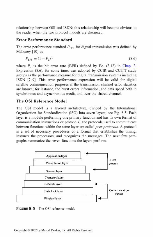
relationship between OSI and ISDN: this relationship will become obvious to
the reader when the two protocol models are discussed.
Error Performance Standard
The error performance standard PEFS for digital transmission was defined by
Mahoney [10] as
PEFS ¼ ð1� PeÞrb ð8:6Þwhere Pe is the bit error rate (BER) defined by Eq. (3.12) in Chap. 3.
Expression (8.6), for some time, was adopted by CCIR and CCITT study
groups as the performance measure for digital transmission systems including
ISDN [7–9]. This error performance expression will be valid for digital
satellite communication purposes if the transmission channel error statistics
are known; for instance, the burst errors information, and data speed both in
synchronous and asynchronous media and over the shared channel.
The OSI Reference Model
The OSI model is a layered architecture, divided by the International
Organization for Standardization (ISO) into seven layers; see Fig. 8.5. Each
layer is a module performing one primary function and has its own format of
communication instructions or protocols. The protocols used to communicate
between functions within the same layer are called peer protocols. A protocol
is a set of necessary procedures or a format that establishes the timing,
instructs the processors, and recognizes the messages. The next few para-
graphs summarize the seven functions the layers perform.
FIGURE 8.5 The OSI reference model.
Copyright © 2002 by Marcel Dekker, Inc. All Rights Reserved.
The OSI layers are divided into two important subsets: the host process
(or customer portion of the system) and the communication subnet (also called
communication subnetwork or the carrier portion of the system). The host
process is comprised of the upper three layers (the session, presentation, and
application layers). The middle layer, the transport layer, is the first end-to-end
layer, which acts as a buffer between the two subsets. In some literature, the
transport layer is grouped with the host process.
The lowest layer of the OSI reference model is the physical layer. It
handles the data transmission between one node (e.g., host workstation) and
the next, monitors data error rates, and defines anything generally associated
with the physical transmission of the bit stream.
The data link layer maintains a reliable communication link between
adjacent nodes. Once communication is established between two nodes, their
data link layers are connected physically through the physical layer and
logically through peer protocols. Data transmissions through this layer are
synchronized so that frames (or packets) are sent in the same sequence as
received.
The network layer creates the logical paths, known as virtual circuits,
along the communication subnet for transmitting data from node to node. Only
the network layer knows the virtual circuits. Switching, routing, and control-
ling the congestion of information frames within the subnet are functions of
this layer.
The transport layer manages the successful node-to-node transportation
of data. This layer handles packet errors, packet order, and other critical
transport issues. The major difference between the data link and transport
layers is that the data link domain lies between adjacent nodes, whereas that of
the transport layer extends from the source node to the destination (or end-to-
end) within the communication subnet.
The transmission link between two nodes is maintained by the session
layer, ensuring that point-to-point transmissions are established and remain
uninterrupted. Once the communication session is finished, this layer
‘‘performs a disconnect’’ between the nodes.
The presentation layer formats and encrypts data to be transmitted
across a network. It provides a data manipulation function, not a communica-
tion function.
The application layer provides application services for end users. These
services include file transfers, file management, e-mail, virtual terminal
emulation, remote database access, and other network software services.
In summary, the OSI reference model of network communications
provides in particular a basis for nodes to communicate within the same
Copyright © 2002 by Marcel Dekker, Inc. All Rights Reserved.
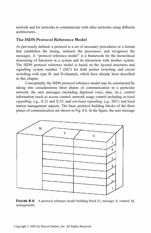
network and for networks to communicate with other networks using different
architectures.
The ISDN Protocol Reference Model
As previously defined, a protocol is a set of necessary procedures or a format
that establishes the timing, instructs the processors, and recognizes the
messages. A ‘‘protocol reference model’’ is a framework for the hierarchical
structuring of functions in a system and its interaction with another system.
The ISDN protocol reference model is based on the layered structures and
signalling system number 7 (SS7) for both packet switching and circuit
switching with type B- and D-channels, which have already been described
in this chapter.
Conceptually, the ISDN protocol reference model may be constructed by
taking into considerations three planes of communication in a particular
network: the user messages (including digitized voice, data, etc.), control
information (such as access control; network usage control including in-band
signalling, e.g., X.21 and X.25; and out-band signalling, e.g., SS7), and local
station management aspects. The basic protocol building blocks of the three
planes of communication are shown in Fig. 8.6. In the figure, the user message
FIGURE 8.6 A protocol reference model building block (U, message; S, control; M,
management).
Copyright © 2002 by Marcel Dekker, Inc. All Rights Reserved.
plane is denoted by U, the control information plane by S, and the manage-
ment plane by M.
The primary function of the U-plane is to convey user information flows,
user-to-user signalling flows, and user management information flows. In
terms of channel structures, the U-plane is associated with the B- or H-
channels but may also involve the D-channels. The U-plane is, in general,
incapable of changing the state of the connection itself.
The main function of the S-plane is to control information flow as well
as the management information flows between a user and a network manage-
ment facility. The S-plane is normally associated with the D-channels. Both
the U- and S-planes are further decomposed into seven layers: numbered from
U-1 to U-7 and S-1 to S-7, respectively. These layers’ flows are conveyed in a
logical sense between peer entities in the appropriate plane of communicating
functional groups.
Physically all the layers’ subflows are transmitted as a single flow over
the physical transmission medium that interconnects the functional groups. To
identify which layer belongs to what, names such as ‘‘network layer’’ or ‘‘data
link layer’’ are used. The functions of each of these layers may be contained in
one or more functional groups that interact with each other across the user-to-
network interface for the purpose of transferring information flows.
Most interactions between the U and S layers go through the manage-
ment plane, M; the exceptions are in the higher layers. The main function of
the M-plane is to manage the U and S resources, facilitate prompt exchanges
of information flows between them, and convey management information to
another system the management application process (MAP).
The preceding discussion allows us to say that a logical transfer of the
subflows (i.e., at the layers level) between functional groups exists and is
governed by peer-to-peer protocols between pairs of U-plane or S-plane
entities. Additionally, the protocol of each layer is independent of the protocol
of the other layer. Consequently, a general ISDN protocol reference model can
be developed with the aid of Fig. 8.7 as follows:
For the reference model within the network segment, different media
connections may be used between two inner building blocks.
The U-plane can be represented by the three lower layers for network
elements that perform information exchange and transfer functions.
The seven layers are used for network elements that perform end-system
functions.
The notation TE in Fig. 8.7 denotes terminal (or station) equipment: a
functional group that includes functions necessary for protocol handling,
Copyright © 2002 by Marcel Dekker, Inc. All Rights Reserved.
FIGURE 8.7 An ISDN protocol reference model.
Copyright ©
2002 by Marcel D
ekker, Inc. All R
ights Reserved.
interfacing, maintenance, and connection to other equipment. S=T is the
signalling point or user=network point whose primary function is to transfer
signalling messages from one signalling link to another. The other codes are as
previously defined. The various information flows exchanged between peer
planes and peer entities in different functional groups are carried over the same
physical medium. The physical and logical interface is the connection point to
external networks. ISDN incorporates the physical, data link, network, and
transport layers of the OSI model. It should be noted that the information flows
could be carried over separate component channels of the existing channel
structure or be multiplexed onto a single component channel.
Advances in technology demand further expansion in the development
of protocols covering full multimedia services (broadband and the Internet).
As such, there is a need for protocols that
Define a universal user-access interface for broadband satellite multi-
media services that (1) is open to different satellite system imple-
mentations and (2) provides both the Internet Protocol (IP) and real-
time seamless broadband service provision
Converge both fixed and mobile multimedia networks toward a global
multimedia mobility architecture; that is, by merging service func-
tions derived from the universal mobile telecommunication system
(UMTS) and the third-generation mobile services (simply called
IMT-2000, mobile multimedia phones, or smart mobiles) and from
fixed broadband access
Separate higher-layer access network functions, which traditionally hide
the lower-layer dependent functions from both the end user and the
core network
Demonstrate how to apply higher-layer access network functions or
layer-dependent functions to other existing satellite access network
functions and planned systems
Allow measurement of quality of service (QoS) and flexibility for
optimized or proprietary air interfaces to satellite systems
8.2.2 Cellular Mobile Systems
An example of a cellular mobile system is the Global System for Mobile
Communications (GSM), which is one of the most successful standardized
systems. The GSM architecture is based on the Public Land Mobile Network
(PLMN), a segment of the land-based digital-switched network (LDSN),
Copyright © 2002 by Marcel Dekker, Inc. All Rights Reserved.
shown in Fig. 8.1. Some of the attributes of mobile communications systems
include [10]
The extensive frequency reuse with a large number of widely dispersed
low-power transmitters located at the base stations
Computer-controlled capabilities to set up automatic handovers from
base station to base station when the signal strength or transmission
distance can be improved to a more acceptable value
The major differences between mobile–satellite communications and land–
mobile communications include path loss, noise environment, and fading
characteristics. Path loss and noise are discussed in Chaps. 3 and 4, and fading
is covered ahead. The functional components comprising mobile communica-
tions are described in Sec. 8.2. Our next task is to describe the basic call setup
for a mobile (cellular) terminal.
Call Setup
When a call is placed, the handset first senses the presence or absence of
cellular frequencies and attempts to place a call through the local cellular
networks if they are available. If cellular service is blocked or not available, the
network operator routes the call through the satellite for an acknowledgment
of the call status. User circuits established through a particular base transceiver
station enter the ground networks (e.g., ISDN) through the satellite gateway
located within the region being served. Call setup is thus established through
an order wire to a mobile switch center (MSC). Often a separate order wire is
assigned to each satellite antenna beam. To make a circuit request, the user
terminal (handset) transmits requests via order wires to satellite. The user (1) is
assigned a beam that provides the strongest signal to the base transceiver
station and (2) is then instructed to use a suitable power level and particular
access technique appropriate to the beam. In some cases with very long calls,
circuit transfer to another satellite is performed without the callers’ participa-
tion.
When the user is moving outside the beam coverage, the call is handed
over to the next beam—a process called handover. For call setup via order
wire, each base station constantly monitors the strength of the modulated
signals it is receiving from each user. When the quality of this signal falls
below certain preassigned norms (values) because the direct path signal may
have been attenuated or the cellular user is moving outside the beam coverage,
the base station sends a request to the centralized cellular switch (MSC) asking
it to attempt a handover. The base station is usually located in the barocenter
(center of the cell) of the service area. The switch then automatically asks each
Copyright © 2002 by Marcel Dekker, Inc. All Rights Reserved.
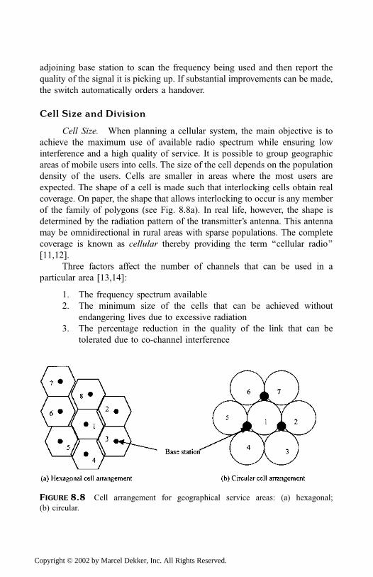
adjoining base station to scan the frequency being used and then report the
quality of the signal it is picking up. If substantial improvements can be made,
the switch automatically orders a handover.
Cell Size and Division
Cell Size. When planning a cellular system, the main objective is to
achieve the maximum use of available radio spectrum while ensuring low
interference and a high quality of service. It is possible to group geographic
areas of mobile users into cells. The size of the cell depends on the population
density of the users. Cells are smaller in areas where the most users are
expected. The shape of a cell is made such that interlocking cells obtain real
coverage. On paper, the shape that allows interlocking to occur is any member
of the family of polygons (see Fig. 8.8a). In real life, however, the shape is
determined by the radiation pattern of the transmitter’s antenna. This antenna
may be omnidirectional in rural areas with sparse populations. The complete
coverage is known as cellular thereby providing the term ‘‘cellular radio’’
[11,12].
Three factors affect the number of channels that can be used in a
particular area [13,14]:
1. The frequency spectrum available
2. The minimum size of the cells that can be achieved without
endangering lives due to excessive radiation
3. The percentage reduction in the quality of the link that can be
tolerated due to co-channel interference
FIGURE 8.8 Cell arrangement for geographical service areas: (a) hexagonal;
(b) circular.
Copyright © 2002 by Marcel Dekker, Inc. All Rights Reserved.
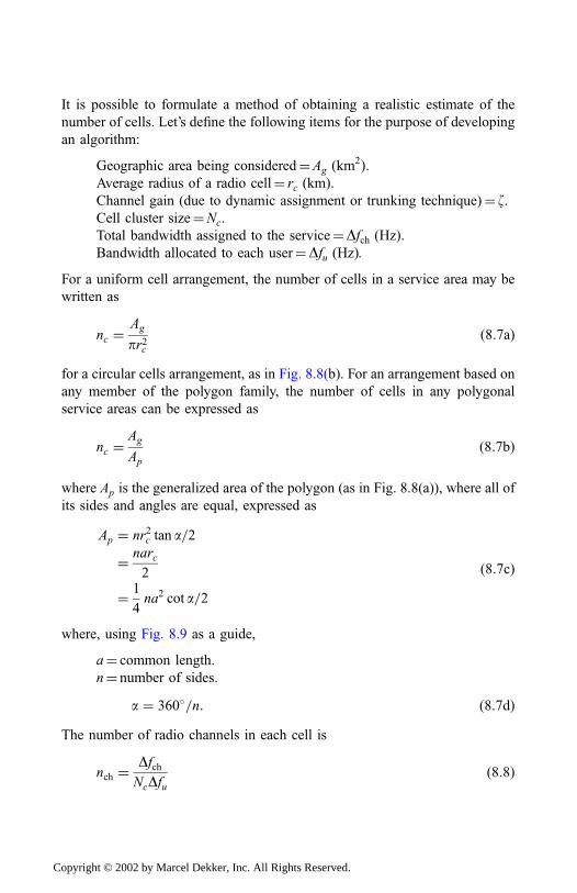
It is possible to formulate a method of obtaining a realistic estimate of the
number of cells. Let’s define the following items for the purpose of developing
an algorithm:
Geographic area being considered¼Ag ðkm2Þ.Average radius of a radio cell¼ rc ðkmÞ.Channel gain (due to dynamic assignment or trunking technique)¼ z.Cell cluster size¼Nc.
Total bandwidth assigned to the service¼Dfch ðHzÞ.Bandwidth allocated to each user¼Dfu ðHzÞ.
For a uniform cell arrangement, the number of cells in a service area may be
written as
nc ¼Ag
pr2cð8:7aÞ
for a circular cells arrangement, as in Fig. 8.8(b). For an arrangement based on
any member of the polygon family, the number of cells in any polygonal
service areas can be expressed as
nc ¼Ag
Ap
ð8:7bÞ
where Ap is the generalized area of the polygon (as in Fig. 8.8(a)), where all of
its sides and angles are equal, expressed as
Ap ¼ nr2c tan a=2
¼ narc
2
¼ 1
4na2 cot a=2
ð8:7cÞ
where, using Fig. 8.9 as a guide,
a¼ common length.
n¼ number of sides.
a ¼ 360�=n: ð8:7dÞThe number of radio channels in each cell is
nch ¼DfchNcDfu
ð8:8Þ
Copyright © 2002 by Marcel Dekker, Inc. All Rights Reserved.
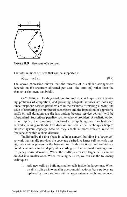
The total number of users that can be supported is
Nusers ¼ ncznch ð8:9ÞThe above expression shows that the success of a cellular arrangement
depends on the spectrum allocated per user—the term Dfu rather than the
channel assignment bandwidth.
Cell Division. Finding a solution to limited radio frequencies, alleviat-
ing problems of congestion, and providing adequate services are not easy.
Since telephone service providers are in the business of making a profit, the
issue of restricting the number of subscribers and the imposition of aggressive
tariffs on call durations are the last options because service delivery will be
substandard. Subscribers penalize such telephone providers. A realistic option
is to improve the economy of networks by applying more sophisticated
network-planning methods. Cell division and smaller cell techniques help to
increase system capacity because they enable a more efficient reuse of
frequencies within a short distance.
Traditionally, the first phase in cellular network building is a larger cell
network that rapidly provides the coverage desired. A larger cell network uses
high transmitter powers in the base station. Both directional and omnidirec-
tional antennas can be deployed according to the required coverage and
frequency reuse demands. When the traffic increases, larger cells can be
divided into smaller ones. When reducing cell size, we can use the following
techniques:
1. Add new cells by building smaller cells inside the larger one. When
a cell is split up into smaller ones, omnidirectional base stations are
replaced by more stations with a larger antenna height and reduced
FIGURE 8.9 Geometry of a polygon.
Copyright © 2002 by Marcel Dekker, Inc. All Rights Reserved.
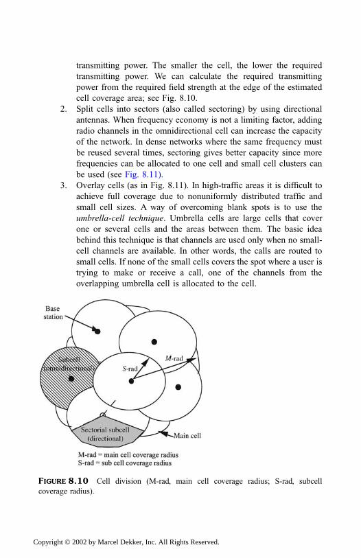
transmitting power. The smaller the cell, the lower the required
transmitting power. We can calculate the required transmitting
power from the required field strength at the edge of the estimated
cell coverage area; see Fig. 8.10.
2. Split cells into sectors (also called sectoring) by using directional
antennas. When frequency economy is not a limiting factor, adding
radio channels in the omnidirectional cell can increase the capacity
of the network. In dense networks where the same frequency must
be reused several times, sectoring gives better capacity since more
frequencies can be allocated to one cell and small cell clusters can
be used (see Fig. 8.11).
3. Overlay cells (as in Fig. 8.11). In high-traffic areas it is difficult to
achieve full coverage due to nonuniformly distributed traffic and
small cell sizes. A way of overcoming blank spots is to use the
umbrella-cell technique. Umbrella cells are large cells that cover
one or several cells and the areas between them. The basic idea
behind this technique is that channels are used only when no small-
cell channels are available. In other words, the calls are routed to
small cells. If none of the small cells covers the spot where a user is
trying to make or receive a call, one of the channels from the
overlapping umbrella cell is allocated to the cell.
FIGURE 8.10 Cell division (M-rad, main cell coverage radius; S-rad, subcell
coverage radius).
Copyright © 2002 by Marcel Dekker, Inc. All Rights Reserved.
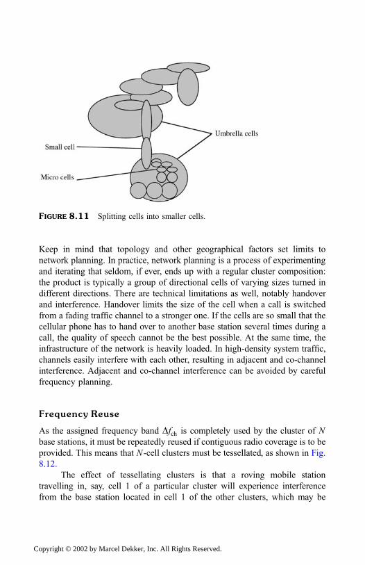
Keep in mind that topology and other geographical factors set limits to
network planning. In practice, network planning is a process of experimenting
and iterating that seldom, if ever, ends up with a regular cluster composition:
the product is typically a group of directional cells of varying sizes turned in
different directions. There are technical limitations as well, notably handover
and interference. Handover limits the size of the cell when a call is switched
from a fading traffic channel to a stronger one. If the cells are so small that the
cellular phone has to hand over to another base station several times during a
call, the quality of speech cannot be the best possible. At the same time, the
infrastructure of the network is heavily loaded. In high-density system traffic,
channels easily interfere with each other, resulting in adjacent and co-channel
interference. Adjacent and co-channel interference can be avoided by careful
frequency planning.
Frequency Reuse
As the assigned frequency band Dfch is completely used by the cluster of N
base stations, it must be repeatedly reused if contiguous radio coverage is to be
provided. This means that N -cell clusters must be tessellated, as shown in Fig.
8.12.
The effect of tessellating clusters is that a roving mobile station
travelling in, say, cell 1 of a particular cluster will experience interference
from the base station located in cell 1 of the other clusters, which may be
FIGURE 8.11 Splitting cells into smaller cells.
Copyright © 2002 by Marcel Dekker, Inc. All Rights Reserved.
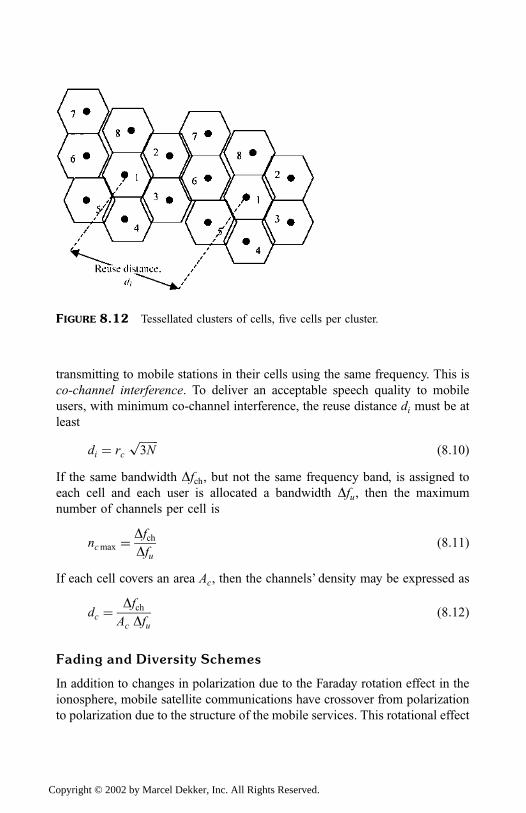
transmitting to mobile stations in their cells using the same frequency. This is
co-channel interference. To deliver an acceptable speech quality to mobile
users, with minimum co-channel interference, the reuse distance di must be at
least
di ¼ rcffiffiffiffiffiffiffi3Np
ð8:10ÞIf the same bandwidth Dfch, but not the same frequency band, is assigned to
each cell and each user is allocated a bandwidth Dfu, then the maximum
number of channels per cell is
ncmax ¼DfchDfu
ð8:11Þ
If each cell covers an area Ac, then the channels’ density may be expressed as
dc ¼DfchAc Dfu
ð8:12Þ
Fading and Diversity Schemes
In addition to changes in polarization due to the Faraday rotation effect in the
ionosphere, mobile satellite communications have crossover from polarization
to polarization due to the structure of the mobile services. This rotational effect
FIGURE 8.12 Tessellated clusters of cells, five cells per cluster.
Copyright © 2002 by Marcel Dekker, Inc. All Rights Reserved.
causes signal fading. Of course, the crossover effect precludes the use of two
different orthogonally polarized waves to increase channel capacity.
A diversity scheme is needed to combat fading. Several diversity
schemes have been employed, including space diversity, frequency diversity,
micro- and macrodiversity, and time diversity. The mode of operation in which
two or more base stations serve the same area is called macrodiversity.
Microdiversity refers to the condition in which two or more signals are
received at one base site or mobile site. Microspace diversity is routinely
used in cellular base sites.
Space diversity can be used to combat short-term fading, whereas
positioning satellites at different locations, not necessarily in the same orbital
plane, can be used to reduce long-term fading. Space-diversity systems
employ two or more antennas spaced a certain distance apart. For example,
a separation of only 30 cm wavelength, which is suitable for implementation
on the mobile side, is sufficient to provide a notable improvement in some
mobile radio channel environments. Macrodiversity is also a form of space
diversity.
Frequency-diversity systems employ two or more different carrier
frequencies to transmit the same information. Statistically, the same informa-
tion signal may or may not fade at the same time at the different carrier
frequencies. An example of a frequency-diversity scheme includes frequency
hopping and very wide band signalling. Time-diversity systems are used
primarily for data transmission. The same data are sent through the radio
channel as many times as necessary until the required quality of transmission
is achieved. An example of this type of scheme is the well-known automatic
repeat request (ARQ).
The improvement of any diversity scheme strongly depends on the
combining techniques employed: the switched combining, feed-forward or
feedback combining, majority vote, and so forth.
8.3 THE INTERNET AND SATELLITES
Satellites have offered broadband services like television or video-on-demand
broadcast, wireless telephone, and electronic mail for years. Developers now
place more emphasis on the speed of delivery of electronic commerce via the
Internet and other telecommunication applications, which makes multimedia
interactivity via the satellite very attractive. This section examines how the
Internet works via the existing land-based integrated digital networks and via
the satellite as well as the technical difficulties that currently prevent rapid
expansion and delivery of these services via the Internet.
Copyright © 2002 by Marcel Dekker, Inc. All Rights Reserved.
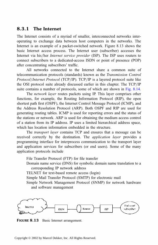
8.3.1 The Internet
The Internet consists of a myriad of smaller, interconnected networks inter-
operating to exchange data between host computers in the networks. The
Internet is an example of a packet-switched network. Figure 8.13 shows the
basic Internet access process. The Internet user (subscriber) accesses the
Internet via his=her Internet service provider (ISP). The ISP uses routers to
connect subscribers to a dedicated-access ISDN or point of presence (POP)
after concentrating subscribers’ traffic.
All networks connected to the Internet share a common suite of
telecommunication protocols (standards) known as the Transmission Control
Protocol=Internet Protocol (TCP=IP). TCP=IP is a layered protocol suite like
the OSI protocol suite already discussed earlier in this chapter. The TCP=IPsuite contains a number of protocols, some of which are shown in Fig. 8.14.
The network layer routes packets using IP. This layer comprises other
functions, for example, the Routing Information Protocol (RIP), the open
shortest path first (OSPF), the Internet Control Message Protocol (ICMP), and
the Address Resolution Protocol (ARP). Both OSPF and RIP are used for
generating routing tables. ICMP is used for reporting errors and the status of
the stations or network. ARP is used for obtaining the medium access control
of a station from its IP address. IP uses a limited hierarchical address space,
which has location information embedded in the structure.
The transport layer contains TCP and ensures that a message can be
received correctly by the destination. The application layer provides a
programming interface for interprocess communication to the transport layer
and application services for subscribers (or end users). Some of the many
application protocols include
File Transfer Protocol (FTP) for file transfer
Domain name service (DNS) for symbolic domain name translation to a
corresponding IP network address
TELNET for text-based remote access (login)
Simple Mail Transfer Protocol (SMTP) for electronic mail
Simple Network Management Protocol (SNMP) for network hardware
and software management
FIGURE 8.13 Basic Internet arrangement.
Copyright © 2002 by Marcel Dekker, Inc. All Rights Reserved.
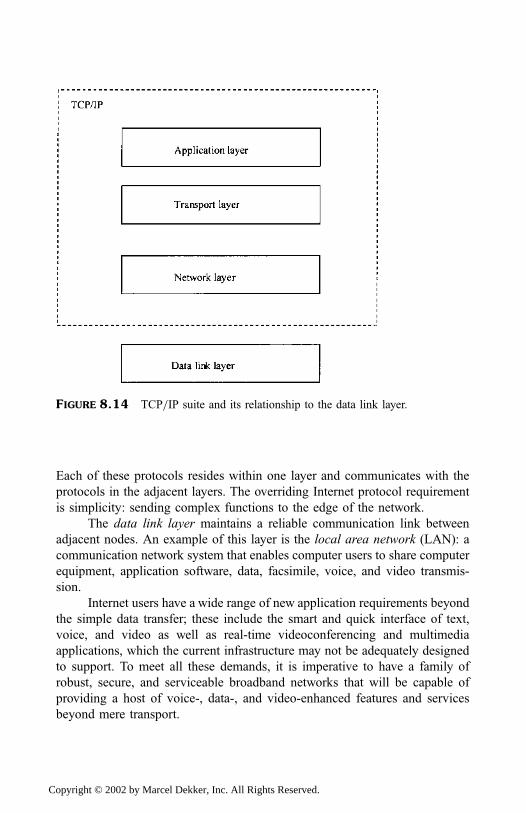
Each of these protocols resides within one layer and communicates with the
protocols in the adjacent layers. The overriding Internet protocol requirement
is simplicity: sending complex functions to the edge of the network.
The data link layer maintains a reliable communication link between
adjacent nodes. An example of this layer is the local area network (LAN): a
communication network system that enables computer users to share computer
equipment, application software, data, facsimile, voice, and video transmis-
sion.
Internet users have a wide range of new application requirements beyond
the simple data transfer; these include the smart and quick interface of text,
voice, and video as well as real-time videoconferencing and multimedia
applications, which the current infrastructure may not be adequately designed
to support. To meet all these demands, it is imperative to have a family of
robust, secure, and serviceable broadband networks that will be capable of
providing a host of voice-, data-, and video-enhanced features and services
beyond mere transport.
FIGURE 8.14 TCP=IP suite and its relationship to the data link layer.
Copyright © 2002 by Marcel Dekker, Inc. All Rights Reserved.
Security
Data security is a matter of great concern to many Internet users. Two broad
types of security have been discussed in the literature and in practice: firewalls
and encryption. A prominent public-key encryption method for e-mail is the
Pretty Good Privacy (PGP), which is based on the Rivest–Shamir–Adleman
(RSA) algorithm [15]. A secured network can be built over the network by
encrypting and decrypting information at both end terminals and stations.
Chapter 1, Sec. 1.4 discusses the principles of encryption and decryption.
Firewalls attempt to provide filters for both incoming and outgoing
packets in order to improve the security of the networks connected to the
Internet. Examples include
Packet filters, which use the IP address and TCP port number to decide
if a packet can pass through the routers. This filter type is used at the
network layer to regulate traffic flow.
Proxy servers (also called circuit-level gateways) prevent direct connec-
tion from the outside to the service on the inside.
Stateful packet inspection (also called dynamic firewall technology) uses
a comparison-basis technique, where a packet under filtering is
compared with the saved state of the previously forwarded packets.
If the record shows that the packet under inspection appears reason-
able, then permission is granted to pass the packet to the intended
destination.
Several firewall products are currently available.
8.3.2 The Internet Via Satellite
Current technology allows the Internet interaction channel to remain within
the ISDN link. Satellite technologies are uniquely poised to address some of
the key challenges that must be met for the Internet to continue its rapid
expansion and advancement: specifically, high-speed access for rural and
remote areas; the distribution and delivery of media-rich content; and tight
integration with existing technologies. With advances in technology and the
miniaturization of electronic components, bidirectional communications can
be carried over satellite, eliminating the necessity of the subscribers’ (end
users’) terrestrial Internet connections that are inherent with the existing one-
way satellite systems.
Figure 8.15 shows a basic Internet access through satellite. The Internet
user (subscriber) accesses the Internet via his=her ISP, which then establishes
Copyright © 2002 by Marcel Dekker, Inc. All Rights Reserved.
access to an Internet point of presence via a gateway station for connection to
the satellite’s network access gateway (NAG). The NAG then sends the
message across the proximate backbone network of the recipient’s ISP,
which is finally delivered to the intended recipient’s address. For this type
of application, channel capacity needs to be shared by different users.
Subscribers’ access to satellite using a subscriber unit (e.g., handheld,
pocket-sized phones) may be the simplest feature of satellite mobile systems of
the future where the subscribers will be able to access voice, facsimile, data,
and paging services with acceptable high quality.
There are direct benefits for users accessing Internet via satellite,
including
Connection through or bypassing terrestrial networks and provision for
direct-to-home services via the digital video broadcasting (DVB) IP.
DVB technology uses multiplexing (e.g., MPEG-2) for data packet-
ing but with different channel modulation. MPEG-2 is the broadcast-
quality compression standard for video communication.
Provision for higher throughput and possibly asymmetric links.
Allowance for multicasting transmission; that is, sending one message to
authorized users instantaneously within the network through a variety
of earth stations.
Provision for faster access (or response) time and delivery of informa-
tion to any inhospitable terrain or region where there is rapidly
expanding customer demand but insufficient terrestrial infrastructure.
Of course, there have been attempts to deliver IP via satellite, but the satellite
technologies have focused on connection-oriented transmission protocols,
which are really suited for voice traffic rather than IP, unnecessarily squander-
ing expensive capacity. What are the challenges ahead for effective delivery of
IP via satellite?
8.3.3 Technical Challenges
The TCP=IP shortcomings in the typical satellite environment include latency
(degradations due to slow-start), data security over the satellite link, and
optimization (window size, traffic acknowledgment for short transmissions
over high-latency channels, as well as scheduling capacity). These short-
comings demand attention in order to provide more efficient, secure, and
application-expansive internetworking via satellite. The issue of data or
Copyright © 2002 by Marcel Dekker, Inc. All Rights Reserved.
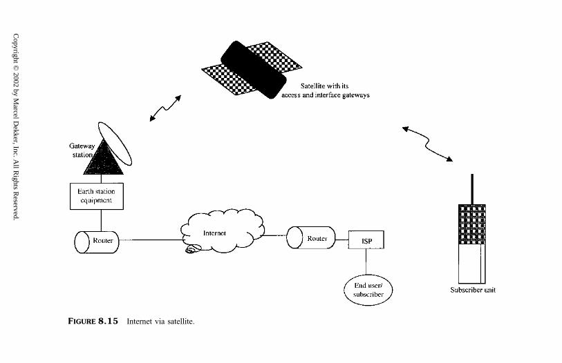
FIGURE 8.15 Internet via satellite.
Copyright ©
2002 by Marcel D
ekker, Inc. All R
ights Reserved.
message security via satellite is discussed in Chap. 1 and earlier in this chapter.
Thus, we examine other TCP=IP challenges in this section.
Latency. Latency is a critical parameter of communication service
quality, particularly for interactive communications and for many standard
data protocols. TCP=IP performs poorly over high-latency or noisy channels.
Bit error rates (BER) of 10�7 can be acceptable in telephone environments,
but this level of performance will render TCP=IP almost unusable. Geo-
stationary satellite links are inherently high-latency and can be noisy. For
example, we note in Chap. 1, Sec. 1.3, that if circuits are positioned in
geosynchronous orbits, they suffer a transmission delay of about 119msec
between an earth terminal and the satellite, resulting in a user-to-user delay of
238msec and an echo delay of 476msec. Latency in voice communications
becomes noticeable with a round-trip delay over 100msec. To overcome the
slow-start this delay causes, an enhanced communications protocol over the
satellite link must be implemented which terminates and re-originates TCP
connections at both ends of the satellite link without sacrificing the discovery
process and still maintaining end-to-end standards compliance [16].
Optimization. Window size and scheduling capacity are optimization
issues, which affect data throughput and network efficiency. Window sizing
works simply by allowing a transmitter to send a number of packets before
waiting for an acknowledgment from the receiver. Typically, the window size
is short in comparison to the 476msec delay of a satellite link; however, it
minimizes the amount of data that would need to be retransmitted when
packets are dropped. This operation dramatically slows down a satellite
connection.
Scheduling capacity as well as the ‘‘burstiness’’ of subscriber traffic over
the satellite link is another area that can potentially reduce data throughput or
network efficiency. There are two common ways of scheduling capacity:
connection-oriented and connectionless, which reflect two different philoso-
phies of link management. Traffic burstiness determines which scheduling
method is appropriate for data transmission.
The connection-oriented method assigns a fixed level of capacity prior to
transmission and reassigns capacity at the completion of a transmission. What
is remarkable about this method is that at least one round-trip delay is required
to both allocate and de-allocate capacity. For long connections such as voice
phone calls, the overhead to set up and tear down links is very small. For short
connections, such as a URL request over a network, the setup and teardown
time can overwhelm any efficiency the existing protocol achieves. The
traditional switched telephone network’s traffic is relatively smooth and is
Copyright © 2002 by Marcel Dekker, Inc. All Rights Reserved.
well suited to this method. The connection-oriented method does not handle
bursty traffic efficiently because bursts potentially slow down by the ceiling on
capacity allocation.
Connectionless refers in part to the way in which capacity is allocated. It
requires no setup and teardown time. An underlying connectionless method is
a multiple-access scheme that allows for random traffic, collision detection,
and an efficient method for handling collisions to avoid channel breakdown.
Traffic characteristic of data networking environments tends to arrive in bursts,
which is suited to a connectionless method. The issue is how to run an efficient
multiple-access scheme that addresses the issue of channel breakdown.
8.4 SUMMARY
The unrelenting growing demand for interactive communications systems
using small handheld terminals has resulted in the provision of mobile satellite
systems services. As demand for networks has evolved, standards organiza-
tions have worked—and still strive—to ensure compatibility of networks and
networking equipment. This chapter discusses the basic architecture of mobile
satellite systems as well as the backbone transmission network, channel types,
channel structures, the OSI and ISDN protocol reference models, and error
performance standards.
Satellites excell in one-to-many communications, reaching remote areas
where it is not profitable to set up a cellular or Internet network for
telecommunications or data transfer. This chapter also examines cellular
network, Internet operating principles and protocols, and system security.
Latency, channel congestion, capacity scheduling, and network optimization
are some of the issues that require solutions to ensure reliable and secure data
transmission via satellite. With rapid advances in technology, lower production
costs, and the insatiable appetite for consumers’ dollars—as well as the
consumers’ demand for rapid, secure, and reliable interactive telecommunica-
tions—the future is bright for communications via satellite.
BIBLIOGRAPHY
1. Duc, N.Q., and Chew, E.K. (1985). ISDN protocol architecture, IEEE Commu-
nications Magazine, 15–22.
Copyright © 2002 by Marcel Dekker, Inc. All Rights Reserved.

REFERENCES
1. Wu, W.W. (1989). Elements of Digital Satellite Communication: Channel Coding
and Integrated Services Digital Satellite Networks. Computer Science Press.
2. Helgert, H.J. (1991). Integrated Services Digital Networks. Addison-Wesley.
3. Hass, T. (1982). International standardization and ISBN. J. Telecommunication
Networks, I, 4.
4. Mahoney, J. (1975). Users’ view of the network. Bell Systems Technical J. 54, 5.
5. Potter, R. (1985). ISDN protocol and architecture models. Computer Networks and
ISDN Systems, vol. 10.
6. Ronayne, J. (1988). The Integrated Services Digital Network: From Concept to
application. Pitman=Wiley.
7. CCITT (1988). Public land mobile network, mobile application part and interfaces,
Recommendations Q1051–Q1063.
8. CCITT (1988). Public land mobile network, interworking with ISDN and PSTN,
Recommendations Q1000–Q1032.
9. CCITT (1983). Study Group XVIII–Report No. R3–R5 for 1981–1984.
10. Anderson, S. (1996). GSM-Interoperable mobile station call processing architec-
ture in mobile and personal satellite communications 2, Proc. European workshop
on Mobile=Personal Satcoms, 247–269.11. Steele, R. (1994). Mobile Radio Communications. Pentech Press.
12. White, G. (1995). Mobile Radio Technology. Newnes.
13. Kangas, S. and Lahtela, K. (1989). Cell division in mobile telephone systems, in
Pan-European mobile communications. IBC Technical Services, 91–95.
14. Kucar, A.D. (1995). Mobile radio—an overview in Cellular Radio and Personal
Communications, Rappaport, ed. IEEE Press.
15. Rivest, R., Shamir, A., and Adleman, L. (1978). A method for obtaining digital
signatures and public-key cryptosystems, Communications for the ACM, 21:2,
120–126.
16. Tachyon (2001). Internet Access Service.
http://www.tachyon.net/Internet_Access.html
PROBLEMS
1. You are consulting for a county that is considering replacing its anti-
quated communications systems. Besides the county’s administrative
center, most of its population is sparsely spread out, with varying terrain.
What questions would you ask before deciding on your recommendations
for the communications network design? Explain the rationale behind
your questions.
2. Explain the differences between the OSI and ISDN reference models.
3. What applications are parts of TCP=IP, and what functions do they
perform?
Copyright © 2002 by Marcel Dekker, Inc. All Rights Reserved.

4. Describe the protocol used on the Internet.
5. Why is a layered architecture used for network communications?
6. Explain the differences between the end-user-to-network interfaces and
their usefulness in the ISDN architecture.
7. What is the difference between ‘‘peer protocol’’ and ‘‘virtual circuit’’ in a
reference model?
8. Is it correct to consider the interconnectivity architecture as two ‘‘half
gateways’’?
9. Design a security system that protects your system from unwarranted
intrusion from other networks and mail-order marketers.
10. What is stored in a routing table?
Copyright © 2002 by Marcel Dekker, Inc. All Rights Reserved.
Appendix A
Notations
The symbols have been chosen as carefully as possible to prevent confusion.
In a few instances, the same symbol was used. When this occurs, a clear
distinction is made in their meaning and where used in the text.
Symbol Definition
A Aperture length in H-plane of a pyramidal horn
Aa Solar array area required for the cells
Ac Area covered by each radio cell
Ae Effective aperture area
Aeq Equivalent surface area of the satellite that is perpendicular to the
orbit velocity
Ag Cellular radio coverage area for circular cells
Ap Cellular radio coverage area for polygonal cells
Copyright © 2002 by Marcel Dekker, Inc. All Rights Reserved.
B Aperture length in E-plane of a pyramidal horn (in Chap. 2) or
channel bandwidth (in other chapters)
C Average carrier power
Cd Coefficient of aerodynamic drag
CCD=FD=TD User capacity in CDMA=FDMA=TDMA system
Cn=x Normalized total capacity for FDMA=CDMA system
D Aperture diameter
Del;Daz Aperture diameters in elevation and azimuth, respectively
F Flux density at the receiver
Fd Force due to aerodynamic drag
Fg Gravitational force acting on the satellite
G Antenna gain or generator matrix (in Chap. 6)
H Entropy
HD Parity check matrix
Hg Altitude of earth station
H0 Freezing height
I ðxiÞ Information associated with source states xiIdi Power of the ith interfering signals on the downlink
I Identity matrix
Iui Power of the ith interfering signals on the uplink
K Number of cells per channel
KD Decryption key
KE Encryption key
L Axial length to apex to the aperture of the conical horn or rain
geometric path length (Chap. 4)
La Number of octets in a cell
Lc Constraint length of the convolutional code
Ll The pyramidal horn shortest length
LET Latitude of the earth station
Lfs Free-space loss
Lp Total path loss
LSAT Latitude of the satellite
LT Total antenna losses
Mr Received decrypted message
Mt Transmitted plaintext message
N Noise power
Nc Cell cluster size
Nf Number of failing system components
NIU Total uplink noise power
N0 Number of components comprising the system at test period
Copyright © 2002 by Marcel Dekker, Inc. All Rights Reserved.
Ns Number of surviving system components
P Arbitrary matrix
Pr Received power
Ps Effective solar system power
PT Total radiated by transmitting source
R Distance from the hypothetical isotropic source or spherical
surface radius
RðtÞ System reliability at time t
Rc Code rate
Re Equatorial radius of the earth
Rr Data transmission rate
Rv Geocentric radius of earth station
S Error syndrome
Sf Semifocal length of an elliptic orbit
Sm Semiminor axis of an elliptic orbit
Sp Semiparameter of an elliptic orbit
T System noise temperature
Ta Antenna temperature
Tb Bit (or burst) duration
Tc Average time between successive channels
Ts Symbol (or frame) duration
X Message data
Y Received codeword
Z Error-prone received codeword
a Semimajor axis of an ellipse (Chap. 2); unpolarized rain attenua-
tion coefficient (Chap. 4); or side of a polygon (Chap. 8)
ac Attenuation coefficient for circularly polarized raindrop
ad Acceleration due to aerodynamic drag
af Loss factor for solar array cells
ap Power attenuation
b Message length
b Unpolarized rain attenuation coefficient
bc Attenuation coefficient for circularly polarized raindrop
c Speed of light
dc Channel density
dH;min Hamming minimum distance
di Frequency band reuse distance
e Eccentricity of an ellipse
ek Number of correctable errors per codeword in the BCH coding
techniques
Copyright © 2002 by Marcel Dekker, Inc. All Rights Reserved.
el Electrical losses of solar cells
fc Incoming signal frequency
fl Local oscillator frequency
g Acceleration due to gravity at the surface of the earth
h Number of octets in the header
h0 Altitude above the subsatellite point on the earth terminal
k Boltzmann’s constant
ke Constant used to emphasise the type of aperture
ks Solar constant
l Number of accesses or users
m Reference bursts
mk Length of shift register
ms Satellite mass
n Block length
nc Number of cells in a designated radio cell area
nch Number of radio channels in a cell
np Number of bursts, accesses, or traffic stations to the frame
pðxÞ Probability of x
pðyÞ Probability of y
pðxj yÞ Probability of transmitting x given that y was received
q Length of burst errors
r Radius distance focus to the orbit path
rb Input digital bit rate of the user (bit=sec)rc Average radius of a radio cell
rr Rain rate
td Transmission delay between an earth terminal and satellite
te Rotation period of the earth
tp Amount of time an earth station is required to communicate with
an orbiting satellite as it passes overhead
ts Orbit period
v Velocity of the satellite with respect to the atmosphere
ws Swath width
a Apex angle for global coverage
aH Magnetic heading of the antenna
b State probability
D Difference in longitude between the earth station and the satellite
Da Deviation angle between true North and North magnetic poles
Dfch Total bandwidth assigned to the service
Dfu Bandwidth allocated to each user
e Error vector
Copyright © 2002 by Marcel Dekker, Inc. All Rights Reserved.

g Central angle
z Channel gain
Z Antenna efficiency (Chap. 2); throughput (Chap. 5)
Zm Solar cells’ conversion efficiency
l Wavelength in free space
lf Average failure rate
y Earth station elevation angle
Y Deviation angle from the electric axis of the antenna
yBW 3-dB antenna beamwidth
yE 3-dB antenna beamwidth in E-plane
yH 3-dB antenna beamwidth in H-plane
yt True elevation angle
ra Atmospheric density
o Angular velocity
Copyright © 2002 by Marcel Dekker, Inc. All Rights Reserved.
Appendix B
Glossary of Terms
Antenna The interface between a free-space electromagnetic
wave and a guided wave. It can also be described as
the input and output interface of a spacecraft.
Antenna illumination The distribution of radio energy across an antenna or
reflector surface. Illumination affects antenna gain.
Distribution of the radio energy depends on the feed
horn.
Aperture The surface area of an antenna that is exposed to a
radiofrequency (RF) signal.
Apogee The highest point along an elliptical orbit where the
orbit is farthest from earth.
Copyright © 2002 by Marcel Dekker, Inc. All Rights Reserved.
Attenuation The power loss between one transmitting source and
the receiver due to path losses.
Bandwidth The range of frequencies required to represent the
information contained in a signal.
Bearer service A type of telecommunication service that provides the
capacity for the transmission of signals between user-
to-network interface.
Bit error rate (BER) An empirical record of a system’s actual bit error
performance.
Cell A short block of information usually of fixed length,
which is identified with a label.
Channel A specific portion of the information-carrying capa-
city of a network interface, and specified by a specific
transmission rate.
Channel structure The structure that defines the maximum digital carry-
ing capacity in terms of bit rates across a network
interface.
Circuit switching The method of transferring information in which
switching and transmission functions are achieved
by permanently allocating a number of channels or
bandwidth between the connections.
Codec A contraction of code and decode.
Code division
multiple access
A multiple-access scheme where stations use spread-
spectrum modulations and orthogonal codes to avoid
interfering with one another.
Common channel
signalling network
The network that provides physical and transmission
capacity for the transfer of connection control signals
between components of an interexchange network.
Communication
satellite
An electronic relay station orbiting in space that picks
up messages transmitted from the ground and retrans-
mits them to a distant location.
Constellation A collection of similar satellites designed to provide
multiple coverage or multiple redundancy.
Copyright © 2002 by Marcel Dekker, Inc. All Rights Reserved.
Cryptography A science that comprises encryption, decryption, and
a cryptographic key management unit.
Cryptographic key
management
The generation, distribution, recognition, and recep-
tion of the cryptographic keys (passwords).
Decoding The process required to reconstruct the data bit
sequence encoded onto the carrier.
Decryption The unlocking of the locked (decrypted) message; the
reverse of encryption.
Demodulation A process by which the original signal is recovered
from a modulated carrier; the reverse of modulation.
Delay Time a signal takes to go from the sending station
through the satellite to the receiving station.
Downlink The space-to-earth telecommunication pathway.
Drag The friction between a moving vehicle through the
earth’s atmosphere opposing the vehicle’s forward
motion.
Earth station A terrestrial terminal that provides a means of trans-
mitting the modulated RF carrier to the satellite within
the uplink frequency spectrum and receiving the RF
carrier from the satellite with the downlink frequency
spectrum. It is the vital link between satellite and
communications users.
Encryption
(enciphering)
The process of converting messages, information, or
data into a form unreadable by anyone except the
intended recipient.
Feed The radiofrequency (RF) input=output device.
Footprint An area on earth illuminated by a satellite antenna. Its
shape and size depend on a number of factors,
including the antenna design and the satellite’s angle
of elevation.
Forward error
correction
A transmission error detection and correction techni-
que that, in addition to detecting errors, also corrects
errors at the receive end of the link.
Copyright © 2002 by Marcel Dekker, Inc. All Rights Reserved.
Frequency division
multiple access
A technique by which the transponder bandwidth is
shared in separate frequency slots.
Frequency reuse Using the same frequency band several times in such a
way as to increase the overall capacity of a network
without increasing the allocated bandwidth.
Functional group A set of functions required for carrying out tasks in
cooperation with another functional element or group.
Gain A measure of amplifier power expressed in watts (W)
or decibel (dB).
Gateway A special switch used to link part of a network.
Geostationary
satellite (GEO)
A satellite placed in the geosynchronous orbit in the
equatorial plane. Although it appears not to be moving
when seen from the earth, its velocity in space is
3.076 km=sec (11,071.9 km=hr).
Gigahertz (GHz) One billion (109) cycles per second.
High elliptical
orbiting satellite
(HEO)
A specialized orbit in which a satellite continuously
swings very close to the earth, loops out into space,
and then repeats its swing-by. It is an elliptical orbit
approximately 18,000–35,000 km above the earth’s
surface, not necessarily above the equator.
Horn An open-ended waveguide designed to radiate maxi-
mum power in one direction. It could also be part of a
feed.
Internet (or
Internetworking)
The interconnection of multiple networks into a
single, large virtual network.
INMARSAT The International Maritime Satellite Organization that
primarily operates telecommunication services for
ships at sea.
ISDN A telecommunications network that provides end-to-
end digital connections to end users and other network
facilities. ISDN stands for ‘‘integrated service digital
network’’.
Copyright © 2002 by Marcel Dekker, Inc. All Rights Reserved.
Intersatellite link
(ISL)
The link between two satellites in the same orbit.
JPEG Stands for ‘‘Joint Photographic Experts Group’’ the
standard used for compressing and decompressing
continuous-tone (color or grayscale) images. The
ISO=IEC JTC1=SC29 Working Group 10 sets this
standard.
Ka Band Frequency range from 18 to 31GHz.
Kbit=sec Data transmission speed of 1000 bit=sec.
Ku band Frequency range from 10.9 to 17GHz.
L-band Frequency range from 0.5 to 1.5 GHz. Also used to
refer to the 950 to 1450MHz used for cellular radio
communications.
Low-earth orbiting
satellite (LEO)
A satellite that orbits the earth in grids, stretching
approximately 160–1600 km above the earth’s surface.
Middle-earth
orbiting satellite
(MEO)
A compromise satellite between the lower orbits and
the geosynchronous orbits; circular and orbits
approximately 8000–18,000 km above the earth’s
surface, not necessarily above the equator.
MPEG Stands for ‘‘Motion Picture Expert Group’’; the stan-
dard used for compressing motion pictures and multi-
media, in contrast to JPEG. The ISO=IEC JTC1=SC29Working Group 11 sets this standard.
Mobile satellite
system (MSS)
A radio communication service between mobile earth
stations and one or more space stations; between
mobile earth stations by means of one or more
space stations; or between space stations.
Modem A converter that performs modulation and demodula-
tion of transmitted data.
Multicasting Sending one message to specific groups of users
within a network.
Multiplexers Devices that are part of the switching matrix in the
satellite communications subsystem, which distribute,
Copyright © 2002 by Marcel Dekker, Inc. All Rights Reserved.
connect, and combine signals for the amplifiers and
antennas.
Multiplexing The ability to access a single transponder circuit by
multiple users.
Network A collection of links and nodes, which provides
connections between two or more defined points to
facilitate communication between them.
Omnidirectional
antenna
An antenna that radiates uniformly in all directions.
Orbit A path, relative to a specified frame of reference,
described by the center of mass of a satellite in space,
subject to gravitational attraction.
Packet switching A data transmission method that divides messages
into standard-sized packets for greater efficiency of
routing and transport through a network.
Perigee The lowest point along an elliptical orbit, where the
satellite is closest to the earth.
Protocol A set of rules specified to ensure that a disciplined and
accurate transmission and exchange of information
occur across a communication channel.
Protocol reference
model
A framework for the hierarchical structuring of func-
tions in a system and its interaction with another
system.
PSTN Stands for ‘‘Public Switched Telephone Networks’’; a
telecommunications network that provides end-to-end
telephone connections to end users and other network
facilities.
Receiver An electronic device that enables the desired modu-
lated signal to be separated from all other signals
coming from an antenna.
Router Same as gateway.
Satellite A sophisticated electronic communications system
positioned in an orbital plane above the earth. Alter-
natively, a body that revolves around another body of
Copyright © 2002 by Marcel Dekker, Inc. All Rights Reserved.
preponderant mass and that has a motion primarily
and permanently determined by the force of attraction
of this body.
Scrambler A device that electronically alters a modulated signal
so that only those recipients equipped with special
decoders can pick up and interpret an undefiled
version of the original signal.
Signalling system A set of protocols for the exchange of signalling
information; for example, SS7.
Signalling transfer
point (S=T)A signalling point whose primary function is to
transfer signalling messages from one signalling link
to another.
Single channel per
carrier
A multiple-access technique in which each distinct
user channel is allocated a specific carrier instead of a
number of channels being multiplexed onto a single
carrier.
Subscriber access
network
The functional part of ISDN that lies between the
enduser or subscriber and common channel signalling
network (CCSN) and interexchange network (IEN).
Teleservice A type of telecommunication service that provides
both bearer capabilities and higher-layer capabilities
for communication between users.
Terminal equipment
(TE)
A functional group that includes functions necessary
for protocol handling, interfacing, maintenance, and
connection with other equipment.
Time division
multiple access
A form of multiple access where a single carrier is
shared by many users. Signals from earth stations
reaching the satellite consecutively are processed in
time segments without overlapping.
Transmitter An electronic device that broadcasts modulated
signals toward one or many distant receivers.
Transponder An electronic device carried onboard a communica-
tion satellite that picks up a signal on one frequency,
amplifies it, and retransmits it on another frequency.
Copyright © 2002 by Marcel Dekker, Inc. All Rights Reserved.
Uplink The earth-to-space telecommunication pathway.
User-to-network
interface
The point of demarcation between the terminal equip-
ment and the network termination.
X.21 A recommendation by CCITT that specifies the inter-
face between a ‘‘data terminal equipment’’ (DTE) and
a ‘‘data-circuit terminal equipment’’ (DCE) for
synchronous operation over public circuit-switched
data networks.
X.25 A recommendation by CCITT that specifies the inter-
face between a ‘‘data terminal equipment’’ (DTE) and
a ‘‘data-circuit terminal equipment’’ (DCE) for opera-
tion in virtual circuit mode over a packet-switched
network.
Copyright © 2002 by Marcel Dekker, Inc. All Rights Reserved.