SAS/STAT 9.3 User's Guide: The VARIOGRAM Procedure (Chapter)
134
SAS/STAT ® 14.1 User’s Guide The VARIOGRAM Procedure
Transcript of SAS/STAT 9.3 User's Guide: The VARIOGRAM Procedure (Chapter)

SAS/STAT® 14.1 User’s GuideThe VARIOGRAMProcedure

This document is an individual chapter from SAS/STAT® 14.1 User’s Guide.
The correct bibliographic citation for this manual is as follows: SAS Institute Inc. 2015. SAS/STAT® 14.1 User’s Guide. Cary, NC:SAS Institute Inc.
SAS/STAT® 14.1 User’s Guide
Copyright © 2015, SAS Institute Inc., Cary, NC, USA
All Rights Reserved. Produced in the United States of America.
For a hard-copy book: No part of this publication may be reproduced, stored in a retrieval system, or transmitted, in any form or byany means, electronic, mechanical, photocopying, or otherwise, without the prior written permission of the publisher, SAS InstituteInc.
For a web download or e-book: Your use of this publication shall be governed by the terms established by the vendor at the timeyou acquire this publication.
The scanning, uploading, and distribution of this book via the Internet or any other means without the permission of the publisher isillegal and punishable by law. Please purchase only authorized electronic editions and do not participate in or encourage electronicpiracy of copyrighted materials. Your support of others’ rights is appreciated.
U.S. Government License Rights; Restricted Rights: The Software and its documentation is commercial computer softwaredeveloped at private expense and is provided with RESTRICTED RIGHTS to the United States Government. Use, duplication, ordisclosure of the Software by the United States Government is subject to the license terms of this Agreement pursuant to, asapplicable, FAR 12.212, DFAR 227.7202-1(a), DFAR 227.7202-3(a), and DFAR 227.7202-4, and, to the extent required under U.S.federal law, the minimum restricted rights as set out in FAR 52.227-19 (DEC 2007). If FAR 52.227-19 is applicable, this provisionserves as notice under clause (c) thereof and no other notice is required to be affixed to the Software or documentation. TheGovernment’s rights in Software and documentation shall be only those set forth in this Agreement.
SAS Institute Inc., SAS Campus Drive, Cary, NC 27513-2414
July 2015
SAS® and all other SAS Institute Inc. product or service names are registered trademarks or trademarks of SAS Institute Inc. in theUSA and other countries. ® indicates USA registration.
Other brand and product names are trademarks of their respective companies.

Chapter 122
The VARIOGRAM Procedure
ContentsOverview: VARIOGRAM Procedure . . . . . . . . . . . . . . . . . . . . . . . . . . . . . . 9846
Introduction to Spatial Prediction . . . . . . . . . . . . . . . . . . . . . . . . . . . . 9847Getting Started: VARIOGRAM Procedure . . . . . . . . . . . . . . . . . . . . . . . . . . . 9847
Preliminary Spatial Data Analysis . . . . . . . . . . . . . . . . . . . . . . . . . . . . 9848Empirical Semivariogram Computation . . . . . . . . . . . . . . . . . . . . . . . . . 9852Autocorrelation Analysis . . . . . . . . . . . . . . . . . . . . . . . . . . . . . . . . . 9855Theoretical Semivariogram Model Fitting . . . . . . . . . . . . . . . . . . . . . . . . 9856
Syntax: VARIOGRAM Procedure . . . . . . . . . . . . . . . . . . . . . . . . . . . . . . . 9861PROC VARIOGRAM Statement . . . . . . . . . . . . . . . . . . . . . . . . . . . . 9861BY Statement . . . . . . . . . . . . . . . . . . . . . . . . . . . . . . . . . . . . . . 9868COMPUTE Statement . . . . . . . . . . . . . . . . . . . . . . . . . . . . . . . . . . 9869COORDINATES Statement . . . . . . . . . . . . . . . . . . . . . . . . . . . . . . . 9874DIRECTIONS Statement . . . . . . . . . . . . . . . . . . . . . . . . . . . . . . . . 9875ID Statement . . . . . . . . . . . . . . . . . . . . . . . . . . . . . . . . . . . . . . . 9875MODEL Statement . . . . . . . . . . . . . . . . . . . . . . . . . . . . . . . . . . . . 9875PARMS Statement . . . . . . . . . . . . . . . . . . . . . . . . . . . . . . . . . . . . 9887NLOPTIONS Statement . . . . . . . . . . . . . . . . . . . . . . . . . . . . . . . . . 9891STORE Statement . . . . . . . . . . . . . . . . . . . . . . . . . . . . . . . . . . . . 9891VAR Statement . . . . . . . . . . . . . . . . . . . . . . . . . . . . . . . . . . . . . . 9892
Details: VARIOGRAM Procedure . . . . . . . . . . . . . . . . . . . . . . . . . . . . . . . 9892Theoretical Semivariogram Models . . . . . . . . . . . . . . . . . . . . . . . . . . . 9892
Characteristics of Semivariogram Models . . . . . . . . . . . . . . . . . . . 9893Nested Models . . . . . . . . . . . . . . . . . . . . . . . . . . . . . . . . . 9897
Theoretical and Computational Details of the Semivariogram . . . . . . . . . . . . . 9897Stationarity . . . . . . . . . . . . . . . . . . . . . . . . . . . . . . . . . . . 9899Ergodicity . . . . . . . . . . . . . . . . . . . . . . . . . . . . . . . . . . . . 9899Anisotropy . . . . . . . . . . . . . . . . . . . . . . . . . . . . . . . . . . . 9900Pair Formation . . . . . . . . . . . . . . . . . . . . . . . . . . . . . . . . . 9900Angle Classification . . . . . . . . . . . . . . . . . . . . . . . . . . . . . . 9902Distance Classification . . . . . . . . . . . . . . . . . . . . . . . . . . . . . 9903Bandwidth Restriction . . . . . . . . . . . . . . . . . . . . . . . . . . . . . 9904Computation of the Distribution Distance Classes . . . . . . . . . . . . . . . 9905Semivariance Computation . . . . . . . . . . . . . . . . . . . . . . . . . . . 9909Empirical Semivariograms and Surface Trends . . . . . . . . . . . . . . . . 9910
Theoretical Semivariogram Model Fitting . . . . . . . . . . . . . . . . . . . . . . . . 9911Parameter Initialization . . . . . . . . . . . . . . . . . . . . . . . . . . . . . 9913

9846 F Chapter 122: The VARIOGRAM Procedure
Parameter Estimates . . . . . . . . . . . . . . . . . . . . . . . . . . . . . . 9915Quality of Fit . . . . . . . . . . . . . . . . . . . . . . . . . . . . . . . . . . 9915Fitting with Matérn Forms . . . . . . . . . . . . . . . . . . . . . . . . . . . 9918
Autocorrelation Statistics . . . . . . . . . . . . . . . . . . . . . . . . . . . . . . . . 9919Autocorrelation Weights . . . . . . . . . . . . . . . . . . . . . . . . . . . . 9919Autocorrelation Statistics Types . . . . . . . . . . . . . . . . . . . . . . . . 9920Interpretation . . . . . . . . . . . . . . . . . . . . . . . . . . . . . . . . . . 9922The Moran Scatter Plot . . . . . . . . . . . . . . . . . . . . . . . . . . . . . 9922
Computational Resources . . . . . . . . . . . . . . . . . . . . . . . . . . . . . . . . 9923Output Data Sets . . . . . . . . . . . . . . . . . . . . . . . . . . . . . . . . . . . . . 9924Displayed Output . . . . . . . . . . . . . . . . . . . . . . . . . . . . . . . . . . . . . 9927ODS Table Names . . . . . . . . . . . . . . . . . . . . . . . . . . . . . . . . . . . . 9929ODS Graphics . . . . . . . . . . . . . . . . . . . . . . . . . . . . . . . . . . . . . . 9930
Examples: VARIOGRAM Procedure . . . . . . . . . . . . . . . . . . . . . . . . . . . . . 9931Example 122.1: Aspects of Semivariogram Model Fitting . . . . . . . . . . . . . . . 9931Example 122.2: An Anisotropic Case Study with Surface Trend in the Data . . . . . . 9941
Analysis with Surface Trend Removal . . . . . . . . . . . . . . . . . . . . . 9945Example 122.3: Analysis without Surface Trend Removal . . . . . . . . . . . . . . . 9955Example 122.4: Covariogram and Semivariogram . . . . . . . . . . . . . . . . . . . 9962Example 122.5: A Box Plot of the Square Root Difference Cloud . . . . . . . . . . . 9966
References . . . . . . . . . . . . . . . . . . . . . . . . . . . . . . . . . . . . . . . . . . . 9969
Overview: VARIOGRAM ProcedureThe VARIOGRAM procedure computes empirical measures of spatial continuity for two-dimensional spatialdata. These measures are a function of the distances between the sample data pairs. When the data are free ofnonrandom (or systematic) surface trends, the estimated continuity measures are the empirical semivarianceand covariance. The procedure also fits permissible theoretical models to the empirical semivariograms, sothat you can use them in subsequent analysis to perform spatial prediction. You can produce plots of theempirical semivariograms in addition to plots of the fitted models. Both isotropic and anisotropic continuitymeasures are available.
PROC VARIOGRAM also provides the Moran’s I and Geary’s c spatial autocorrelation statistics, in additionto the Moran scatter plot to visualize spatial associations within a specified neighborhood around observa-tions. The procedure produces the OUTVAR=, OUTPAIR=, and OUTDISTANCE= data sets that containinformation about the semivariogram analysis. Also, the OUTACWEIGHTS= and the OUTMORAN= outputdata sets contain information about the autocorrelation analysis.
The VARIOGRAM procedure uses ODS Graphics to create graphs as part of its output. For generalinformation about ODS Graphics, see Chapter 21, “Statistical Graphics Using ODS.” For more informationabout the graphics available in PROC VARIOGRAM, see the section “ODS Graphics” on page 9930.

Introduction to Spatial Prediction F 9847
Introduction to Spatial PredictionMany activities in science and technology involve measurements of one or more quantities at given spatiallocations, with the goal of predicting the measured quantities at unsampled locations. Application areasinclude reservoir prediction in mining and petroleum exploration, in addition to modeling in a broad spectrumof fields (for example, environmental health, environmental pollution, natural resources and energy, hydrology,and risk analysis). Often, the unsampled locations are on a regular grid, and the predictions are used toproduce surface plots or contour maps.
The preceding tasks fall within the scope of spatial prediction, which, in general, is any prediction methodthat incorporates spatial dependence. The study of these tasks involves naturally occurring uncertaintiesthat cannot be ignored. Stochastic analysis frameworks and methods are often used to account for theseuncertainties. Hence, the terms stochastic spatial prediction and stochastic modeling are also used tocharacterize this type of analysis.
A popular method of spatial prediction is ordinary kriging, which produces both predicted values andassociated standard errors. Ordinary kriging requires the complete specification (the form and parametervalues) of the spatial dependence that characterizes the spatial process. For this purpose, models for thespatial dependence are expressed in terms of the distance between any two locations in the spatial domain ofinterest. These models take the form of a covariance or semivariance function.
Spatial prediction, then, involves two steps. First, you model the covariance or semivariance of the spatialprocess. These measures are typically not known in advance. This step involves computing an empiricalestimate, in addition to determining both the mathematical form and the values of any parameters for atheoretical form of the dependence model. Second, you use this dependence model to solve the krigingsystem at a specified set of spatial points, resulting in predicted values and associated standard errors.
SAS/STAT software has two procedures that correspond to these steps for spatial prediction of two-dimensional data. The VARIOGRAM procedure is used in the first step (that is, calculating and modelingthe dependence model), and the KRIGE2D procedure performs the kriging operations to produce the finalpredictions.
This introduction concludes with a note on terminology. You might commonly encounter the terms estimationand prediction used interchangeably by experts in different fields; this could be a source of confusion. Aprecise statistical vernacular uses the term estimation to refer to inferences about the value of fixed butunknown parameters, whereas prediction concerns inferences about the value of random variables—see,for example, Cressie (1993, p. 106). In light of these definitions, kriging methods are clearly predictivetechniques, since they are concerned with making inferences about the value of a spatial random field atobserved or unobserved locations. The SAS/STAT suite of procedures for spatial analysis and prediction(VARIOGRAM, KRIGE2D, and SIM2D) follows the statistical vernacular in the use of the terms estimationand prediction.
Getting Started: VARIOGRAM ProcedurePROC VARIOGRAM uses your data to compute the empirical semivariogram. This computation refers tothe steps you take to derive the empirical semivariance from the data, and then to produce the correspondingsemivariogram plot.

9848 F Chapter 122: The VARIOGRAM Procedure
You can proceed further with the semivariogram analysis if the data are free of systematic trends. Inthat case, you can use the empirical outcome to determine a theoretical semivariogram model by usingthe automated methods provided by the VARIOGRAM procedure. The model characterizes the type oftheoretical semivariance function you use to describe spatial dependence in your data set.
Graphical displays are requested by enabling ODS Graphics. For general information about ODS Graphics,see Chapter 21, “Statistical Graphics Using ODS.” For specific information about the graphics available inthe VARIOGRAM procedure, see the section “ODS Graphics” on page 9930.
Preliminary Spatial Data AnalysisThe thick data set is available from the Sashelp library. The data set simulates measurements of coal seamthickness (in feet) taken over an approximately square area. The Thick variable has the thickness values inthe thick data set. The coordinates are offsets from a point in the southwest corner of the measurement area,with the north and east distances in units of thousands of feet.
It is instructive to see the locations of the measured points in the area where you want to perform spatialprediction. It is desirable to have the sampling locations scattered evenly throughout the prediction area. Ifthe locations are not scattered evenly, the prediction error might be unacceptably large where measurementsare sparse.
You can run PROC VARIOGRAM in this preliminary analysis to determine potential problems. In thefollowing statements, the NOVARIOGRAM option in the COMPUTE statement specifies that only thedescriptive summaries and a plot of the raw data be produced.
title 'Spatial Correlation Analysis with PROC VARIOGRAM';
ods graphics on;
proc variogram data=sashelp.thick plots=pairs(thr=30);compute novariogram nhc=20;coordinates xc=East yc=North;var Thick;
run;
PROC VARIOGRAM produces the table in Figure 122.1 that shows the number of Thick observations readand used. This table provides you with useful information in case you have missing values in the input data.
Figure 122.1 Number of Observations for the thick Data Set
Spatial Correlation Analysis with PROC VARIOGRAM
The VARIOGRAM Procedure
Dependent Variable: Thick
Spatial Correlation Analysis with PROC VARIOGRAM
The VARIOGRAM Procedure
Dependent Variable: Thick
Number of Observations Read 75
Number of Observations Used 75
Then, the scatter plot of the observed data is produced as shown in Figure 122.2. According to the figure,although the locations are not ideally spread around the prediction area, there are not any extended areas

Preliminary Spatial Data Analysis F 9849
lacking measurements. The same graph also provides the values of the measured variable by using coloredmarkers.
Figure 122.2 Scatter Plot of the Observations Spatial Distribution
The following is a crucial step. Any obvious surface trend must be removed before you compute the empiricalsemivariogram and proceed to estimate a model of spatial dependence (the theoretical semivariogram model).You can observe in Figure 122.2 the small-scale variation typical of spatial data, but a first inspection indicatesno obvious major systematic trend.
Assuming, therefore, that the data are free of surface trends, you can work with the original thickness ratherthan residuals obtained from a trend removal process. The following analysis also assumes that the spatialcharacterization is independent of the direction of the line that connects any two equidistant pairs of data;this is a property known as isotropy. See “Example 122.2: An Anisotropic Case Study with Surface Trend inthe Data” on page 9941 for a more detailed approach to trend analysis and the issue of anisotropy.
Following the previous exploratory analysis, you then need to classify each data pair as a member of a distanceinterval (lag). PROC VARIOGRAM performs this grouping with two required options for semivariogramcomputation: the LAGDISTANCE= and MAXLAGS= options. These options are based on your assessmentof how to group the data pairs within distance classes.
9850 F Chapter 122: The VARIOGRAM Procedure
The meaning of the required LAGDISTANCE= option is as follows. Classify all pairs of points into intervalsaccording to their pairwise distance. The width of each distance interval is the LAGDISTANCE= value. Themeaning of the required MAXLAGS= option is simply the number of intervals you consider. The problemis that given only the scatter plot of the measurement locations, it is not clear what values to give to theLAGDISTANCE= and MAXLAGS= options.
Ideally, you want a sufficient number of distance classes that capture the extent to which your data arecorrelated and you want each class to contain a minimum of data pairs to increase the accuracy in yourcomputations. A rule of thumb used in semivariogram computations is that you should have at least 30 pairsper lag class. This is an empirical arbitrary threshold; see the section “Choosing the Size of Classes” onpage 9907 for further details.
In the preliminary analysis, you use the option NHCLASSES= in the COMPUTE statement to help youexperiment with these numbers and choose values for the LAGDISTANCE= and MAXLAGS= options. Here,in particular, you request NHCLASSES=20 to preview a classification that uses 20 distance classes acrossyour spatial domain. A zero lag class is always considered; therefore the output shows the number of distanceclasses to be one more than the number you specified.
Based on your selection of the NHCLASSES= option, the NOVARIOGRAM option produces a pairwise dis-tances table from your observations shown in Figure 122.3, and the corresponding histogram in Figure 122.4.For illustration purposes, you also specify a threshold of minimum data pairs per distance class in the PAIRSoption as THR=30. As a result, a reference line appears in the histogram so that you can visually identify anylag classes with pairs that fall below your specified threshold.
Figure 122.3 Pairwise Distance Intervals Table
Pairwise Distance Intervals
LagClass Bounds
Numberof Pairs
Percentageof Pairs
0 0.00 3.48 7 0.25%
1 3.48 10.45 81 2.92%
2 10.45 17.42 138 4.97%
3 17.42 24.39 167 6.02%
4 24.39 31.36 204 7.35%
5 31.36 38.33 210 7.57%
6 38.33 45.30 213 7.68%
7 45.30 52.27 253 9.12%
8 52.27 59.24 237 8.54%
9 59.24 66.20 280 10.09%
10 66.20 73.17 252 9.08%
11 73.17 80.14 230 8.29%
12 80.14 87.11 217 7.82%
13 87.11 94.08 154 5.55%
14 94.08 101.05 71 2.56%
15 101.05 108.02 41 1.48%
16 108.02 114.99 14 0.50%
17 114.99 121.96 5 0.18%
18 121.96 128.93 1 0.04%
19 128.93 135.89 0 0.00%
20 135.89 142.86 0 0.00%
Preliminary Spatial Data Analysis F 9851
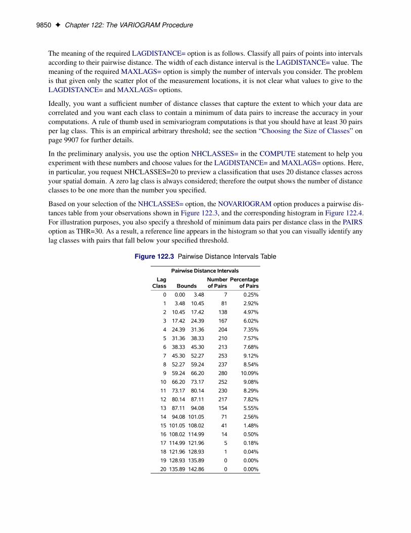
The NOVARIOGRAM option also produces a table with useful facts about the pairs and the distancesbetween the most remote data in selected directions, shown in Figure 122.5. In particular, the lag distancevalue is calculated based on your selection of the NHCLASSES= option. The last three table entries reportthe overall maximum distance among your data pairs, in addition to the maximum distances in the main axesdirections—that is, the vertical (N–S) axis and the horizontal (E–W) axis. This information is also providedin the inset of Figure 122.4. When you specify a threshold in the PAIRS suboption of the PLOTS option, asin this example, the threshold also appears in the table. Then, the line that follows indicates the highest lagclass with the following property: each one of the distance classes that lie farther away from this lag featuresa pairs population below the specified threshold.
With the preceding information you can determine appropriate values for the LAGDISTANCE= andMAXLAGS= options in the COMPUTE statement. In particular, the classification that uses 20 distanceclasses is satisfactory, and you can choose LAGDISTANCE=7 after following the suggestion in Figure 122.5.
Figure 122.4 Distribution of Pairwise Distances

9852 F Chapter 122: The VARIOGRAM Procedure
Figure 122.5 Pairs Information Table
Pairs Information
Number of Lags 21
Lag Distance 6.97
Minimum Pairs Threshold 30
Highest Lag With Pairs > Threshold 15
Maximum Data Distance in East 97.50
Maximum Data Distance in North 99.60
Maximum Data Distance 139.38
The MAXLAGS= option needs to be specified based on the spatial extent to which your data are correlated.Unless you know this size, in the present omnidirectional case you can assume the correlation extent to beroughly equal to half the overall maximum distance between data points.
The table in Figure 122.5 suggests that this number corresponds to 139,380 feet, which is most likely on orclose to a diagonal direction (that is, the northeast–southwest or northwest–southeast direction). Hence, youcan expect the correlation extent in this scale to be around 139:4=2 D 69; 700 feet. Consequently, considerlag classes up to this distance for the empirical semivariogram computations. Given your lag size selection,Figure 122.3 indicates that this distance corresponds to about 10 lags; hence you can set MAXLAGS=10.
Overall, for a specific NHCLASSES= choice of class count, you can expect your choice of MAXLAGS=to be approximately half the number of the lag classes (see the section “Spatial Extent of the EmpiricalSemivariogram” on page 9908 for more details).
After you have starting values for the LAGDISTANCE= and MAXLAGS= options, you can run the VARI-OGRAM procedure multiple times to inspect and compare the results you get by specifying different valuesfor these options.
Empirical Semivariogram ComputationUsing the values of LAGDISTANCE=7 and MAXLAGS=10 computed previously, rerun PROC VARI-OGRAM without the NOVARIOGRAM option in order to compute the empirical semivariogram. Youspecify the CL option in the COMPUTE statement to calculate the 95% confidence limits for the classicalsemivariance. The section “COMPUTE Statement” on page 9869 describes how to use the ALPHA= optionto specify a different confidence level.
Also, you can request a robust version of the semivariance with the ROBUST option in the COMPUTEstatement. PROC VARIOGRAM produces a plot that shows both the classical and the robust empiricalsemivariograms. See the details of the PLOTS option to specify different instances of plots of the empiricalsemivariogram. The following statements implement the preceding requests:

Empirical Semivariogram Computation F 9853
proc variogram data=sashelp.thick outv=outv;compute lagd=7 maxlag=10 cl robust;coordinates xc=East yc=North;var Thick;
run;
Figure 122.6 displays the PROC VARIOGRAM output empirical semivariogram table for the precedingstatements. The table displays a total of eleven lag classes, even though you specified MAXLAGS=10. TheVARIOGRAM procedure always includes a zero lag class in the computations in addition to the MAXLAGSclasses you request with the MAXLAGS= option. Hence, semivariance is actually computed at MAXLAGS+1lag classes; see the section “Distance Classification” on page 9903 for more details.
Figure 122.6 Output Table for the Empirical Semivariogram Analysis
Spatial Correlation Analysis with PROC VARIOGRAM
The VARIOGRAM Procedure
Dependent Variable: Thick
Spatial Correlation Analysis with PROC VARIOGRAM
The VARIOGRAM Procedure
Dependent Variable: Thick
Empirical Semivariogram
Semivariance
LagClass
PairCount
AverageDistance Robust Classical
StandardError
95%Confidence
Limits
0 7 2.64 0.028 0.034 0.018 0 0.069
1 82 7.29 0.210 0.394 0.061 0.273 0.514
2 138 14.16 1.008 1.179 0.142 0.901 1.458
3 169 21.08 3.018 2.799 0.304 2.202 3.396
4 205 27.93 4.811 4.602 0.455 3.711 5.493
5 213 35.17 5.990 5.928 0.574 4.802 7.054
6 214 42.20 8.104 7.518 0.727 6.094 8.943
7 250 48.78 7.533 7.221 0.646 5.955 8.487
8 247 56.16 8.066 7.195 0.647 5.926 8.464
9 281 62.89 8.279 6.845 0.577 5.713 7.976
10 250 69.93 8.144 6.358 0.569 5.243 7.472
Figure 122.7 shows both the classical and robust empirical semivariograms. In addition, the plot features theapproximate 95% confidence limits for the classical semivariance. The figure exhibits a typical behavior ofthe computed semivariance uncertainty, where in general the variance increases with distance from the originat Distance=0.

9854 F Chapter 122: The VARIOGRAM Procedure
Figure 122.7 Classical and Robust Empirical Semivariograms for Coal Seam Thickness Data
The needle plot in the lower part of the Figure 122.7 provides the number of pairs that were used in thecomputation of the empirical semivariance for each lag class shown. In general, this is a pairwise distributionthat is different from the distribution depicted in Figure 122.4. First, the number of pairs shown in the needleplot depends on the particular criteria you specify in the COMPUTE statement of PROC VARIOGRAM.Second, the distances shown for each lag on the Distance axis are not the midpoints of the lag classes as inthe pairwise distances plot, but rather the average distance from the origin Distance=0 of all pairs in a givenlag class.

Autocorrelation Analysis F 9855
Autocorrelation AnalysisYou can use the autocorrelation analysis features of PROC VARIOGRAM to compute the autocorrelationMoran’s I and Geary’s c statistics and to obtain the Moran scatter plot. In the following statements, you askfor the Moran’s I and Geary’s c statistics under the assumption of randomization using binary weights, inaddition to the Moran scatter plot:
proc variogram data=sashelp.thick outv=outv plots(only)=moran;compute lagd=7 maxlag=10 autocorr(assum=random);coordinates xc=East yc=North;var Thick;
run;
For the autocorrelation analysis with binary weights and the Moran scatter plot, the LAGDISTANCE= optionindicates that you consider as neighbors of an observation all other observations within the specified distancefrom it.
Figure 122.8 shows the output from the requested autocorrelation analysis. This includes the observed(computed) Moran’s I and Geary’s c coefficients, the expected value and standard deviation for each coeffi-cient, the corresponding Z score, and the p-value in the Pr >j Z j column. The low p-values suggest strongautocorrelation for both statistics types. A two-sided p-value is reported, which is the probability that theobserved coefficient lies farther away from j Z j on either side of the coefficient’s expected value—that is,lower than –Z or higher than Z. The sign of Z for both Moran’s I and Geary’s c coefficients indicates positiveautocorrelation in the Thick data values; see the section “Interpretation” on page 9922 for more details.
Figure 122.8 Output Table for the Autocorrelation Statistics
Spatial Correlation Analysis with PROC VARIOGRAM
The VARIOGRAM Procedure
Dependent Variable: Thick
Spatial Correlation Analysis with PROC VARIOGRAM
The VARIOGRAM Procedure
Dependent Variable: Thick
Autocorrelation Statistics
Assumption Coefficient Observed ExpectedStdDev Z Pr > |Z|
Randomization Moran's I 0.9240 -0.0244 0.145 6.53 <.0001
Randomization Geary's c 0.0162 1.0000 0.175 -5.62 <.0001
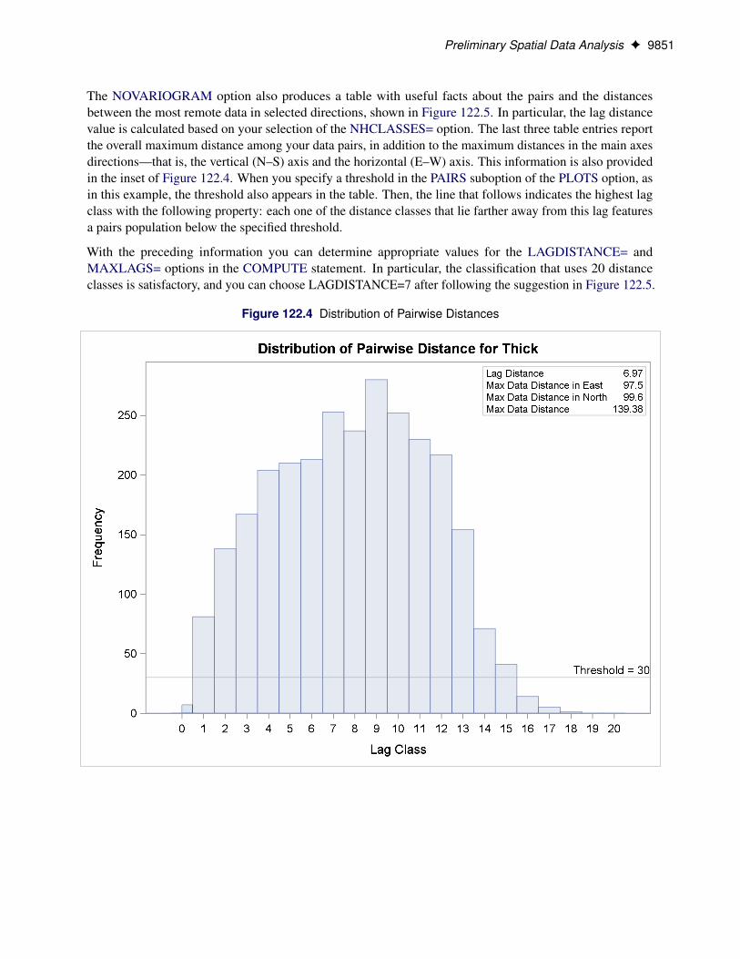
The requested Moran scatter plot is shown in Figure 122.9. The plot includes all nonmissing observations thathave neighbors within the specified LAGDISTANCE= distance. The horizontal axis displays the standardizedThick values, and the vertical axis displays the corresponding weighted average of their neighbors. The plotdata points are concentrated in the upper right and lower left quadrants defined by the lines x = 0 and y =0, and clearly around the axes’ diagonal reference line y = x of slope 1. This fact indicates strong positivespatial association in the thick data set observations. Therefore, for each observation its neighbors withinthe specified LAGDISTANCE= distance have overall similar Thick values to that observation. The plotalso displays the linear regression slope, whose value is the Moran’s I coefficient when the binary weightsare row-averaged. See the section “The Moran Scatter Plot” on page 9922 for more details about the Moranscatter plot.
9856 F Chapter 122: The VARIOGRAM Procedure
Figure 122.9 Moran Scatter Plot for Coal Seam Thickness Data
Theoretical Semivariogram Model FittingPROC VARIOGRAM features automated semivariogram fitting. In particular, the procedure selects atheoretical semivariogram model to fit the empirical semivariance and produces estimates of the modelparameters in addition to a fit plot. You have the option to save these estimates in an item store, which is abinary file format that is defined by the SAS System and that you cannot modify. Then, you can retrieve thisinformation at a later point from the item store for future analysis with PROC KRIGE2D or PROC SIM2D.
The coal seam thickness empirical semivariogram in Figure 122.7 shows first a slow, then rapid, rise from theorigin. This behavior suggests that you can approximate the empirical semivariance with a Gaussian-typeform
z.h/ D c0
"1 � exp
�h2
a20
!#

Theoretical Semivariogram Model Fitting F 9857
as shown in the section “Theoretical Semivariogram Models” on page 9892. Based on this remark, youchoose to fit a Gaussian model to your classical semivariogram. Run PROC VARIOGRAM again and specifythe MODEL statement with the FORM=GAU option. By default, PROC VARIOGRAM uses the weightedleast squares (WLS) method to fit the specified model, although you can explicitly specify the METHOD=option to request the fitting method. You want additional information about the estimated parameters, soyou specify the CL option in the MODEL statement to compute their 95% confidence limits and the COVBoption of the MODEL statement to produce a table with their approximate covariances. You also specify theSTORE statement to save the fitting outcome into an item store file with the name SemivStoreGau and adesired label. You run the following statements:
proc variogram data=sashelp.thick outv=outv;store out=SemivStoreGau / label='Thickness Gaussian WLS Fit';compute lagd=7 maxlag=10;coordinates xc=East yc=North;model form=gau cl / covb;var Thick;
run;
ods graphics off;
After you run the procedure you get a series of output objects from the fitting analysis. In particular,Figure 122.10 shows first a model fitting table with the name and a short label of the model that you requestedto use for the fit. The table also displays the name and label of the specified item store.
Figure 122.10 Semivariogram Model Fitting General Information
Spatial Correlation Analysis with PROC VARIOGRAM
The VARIOGRAM Procedure
Dependent Variable: ThickAngle: Omnidirectional
Current Model: Gaussian
Spatial Correlation Analysis with PROC VARIOGRAM
The VARIOGRAM Procedure
Dependent Variable: ThickAngle: Omnidirectional
Current Model: Gaussian
Semivariogram Model Fitting
Name Gaussian
Label Gau
Output Item Store WORK.SEMIVSTOREGAU
Item Store Label Thickness Gaussian WLS Fit
If you specify no parameters, as in the current example, then PROC VARIOGRAM initializes the modelparameters for you with default values based on the empirical semivariance; for more details, see the section“Theoretical Semivariogram Model Fitting” on page 9911. The initial values provided by the VARIOGRAMprocedure for the Gaussian model are displayed in the table in Figure 122.11.
Figure 122.11 Semivariogram Fitting Model Information
Model Information
ParameterInitialValue
Nugget 0
Scale 6.7992
Range 34.9635
9858 F Chapter 122: The VARIOGRAM Procedure
Otherwise, in PROC VARIOGRAM you can specify initial values for parameters with the PARMS statement.Alternatively, you can specify fixed values for the model scale and range with the SCALE= and RANGE=options, respectively, in the MODEL statement. A nugget effect is always used in model fitting. Unless youexplicitly specify a fixed nugget effect with the NUGGET= option in the MODEL statement or initialize thenugget parameter in the PARMS statement, the nugget effect is automatically initialized to zero. See thesection “Syntax: VARIOGRAM Procedure” on page 9861 for more details about how the MODEL statementand the PARMS statement handle model parameters.
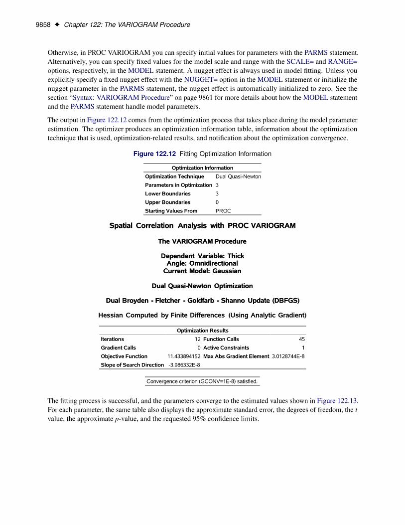
The output in Figure 122.12 comes from the optimization process that takes place during the model parameterestimation. The optimizer produces an optimization information table, information about the optimizationtechnique that is used, optimization-related results, and notification about the optimization convergence.
Figure 122.12 Fitting Optimization Information
Optimization Information
Optimization Technique Dual Quasi-Newton
Parameters in Optimization 3
Lower Boundaries 3
Upper Boundaries 0
Starting Values From PROC
Spatial Correlation Analysis with PROC VARIOGRAM
The VARIOGRAM Procedure
Dependent Variable: ThickAngle: Omnidirectional
Current Model: Gaussian
Dual Quasi-Newton Optimization
Dual Broyden - Fletcher - Goldfarb - Shanno Update (DBFGS)
Spatial Correlation Analysis with PROC VARIOGRAM
The VARIOGRAM Procedure
Dependent Variable: ThickAngle: Omnidirectional
Current Model: Gaussian
Dual Quasi-Newton Optimization
Dual Broyden - Fletcher - Goldfarb - Shanno Update (DBFGS)
Hessian Computed by Finite Differences (Using Analytic Gradient)
Optimization Results
Iterations 12 Function Calls 45
Gradient Calls 0 Active Constraints 1
Objective Function 11.433894152 Max Abs Gradient Element 3.0128744E-8
Slope of Search Direction -3.986332E-8
Convergence criterion (GCONV=1E-8) satisfied.
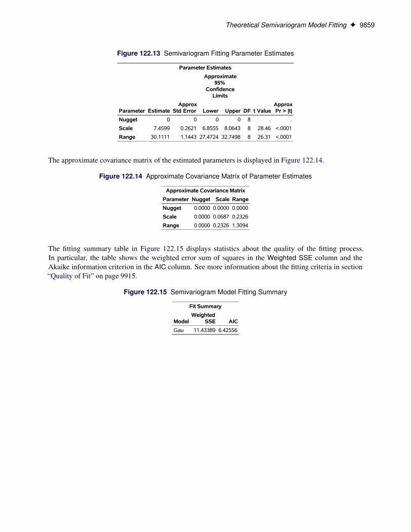
The fitting process is successful, and the parameters converge to the estimated values shown in Figure 122.13.For each parameter, the same table also displays the approximate standard error, the degrees of freedom, the tvalue, the approximate p-value, and the requested 95% confidence limits.
Theoretical Semivariogram Model Fitting F 9859
Figure 122.13 Semivariogram Fitting Parameter Estimates
Parameter Estimates
Approximate95%
ConfidenceLimits
Parameter EstimateApprox
Std Error Lower Upper DF t ValueApproxPr > |t|
Nugget 0 0 0 0 8 . .
Scale 7.4599 0.2621 6.8555 8.0643 8 28.46 <.0001
Range 30.1111 1.1443 27.4724 32.7498 8 26.31 <.0001
The approximate covariance matrix of the estimated parameters is displayed in Figure 122.14.
Figure 122.14 Approximate Covariance Matrix of Parameter Estimates
Approximate Covariance Matrix
Parameter Nugget Scale Range
Nugget 0.0000 0.0000 0.0000
Scale 0.0000 0.0687 0.2326
Range 0.0000 0.2326 1.3094
The fitting summary table in Figure 122.15 displays statistics about the quality of the fitting process.In particular, the table shows the weighted error sum of squares in the Weighted SSE column and theAkaike information criterion in the AIC column. See more information about the fitting criteria in section“Quality of Fit” on page 9915.
Figure 122.15 Semivariogram Model Fitting Summary
Fit Summary
ModelWeighted
SSE AIC
Gau 11.43389 6.42556
9860 F Chapter 122: The VARIOGRAM Procedure
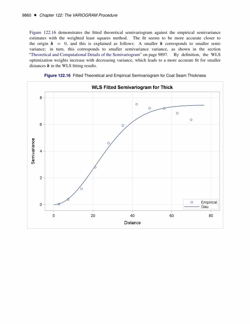
Figure 122.16 demonstrates the fitted theoretical semivariogram against the empirical semivarianceestimates with the weighted least squares method. The fit seems to be more accurate closer tothe origin h D 0, and this is explained as follows: A smaller h corresponds to smaller semi-variance; in turn, this corresponds to smaller semivariance variance, as shown in the section“Theoretical and Computational Details of the Semivariogram” on page 9897. By definition, the WLSoptimization weights increase with decreasing variance, which leads to a more accurate fit for smallerdistances h in the WLS fitting results.
Figure 122.16 Fitted Theoretical and Empirical Semivariogram for Coal Seam Thickness

PROC VARIOGRAM Statement F 9861
Syntax: VARIOGRAM ProcedureThe following statements are available in the VARIOGRAM procedure:
PROC VARIOGRAM options ;BY variables ;COMPUTE computation-options ;COORDINATES coordinate-variables ;DIRECTIONS directions-list ;ID variable ;MODEL model-options ;PARMS parameters-list < / parameters-options > ;NLOPTIONS < options > ;STORE store-options ;VAR analysis-variables-list ;
The COMPUTE and COORDINATES statements are required. The MODEL and PARMS statements arehierarchical. If you specify a PARMS statement, it must follow a MODEL statement.
PROC VARIOGRAM StatementPROC VARIOGRAM options ;
The PROC VARIOGRAM statement invokes the VARIOGRAM procedure. Table 122.1 summarizes theoptions available in the PROC VARIOGRAM statement.
Table 122.1 PROC VARIOGRAM Statement Options
Option Description
DATA= Specifies the input data setIDGLOBAL Labels observations across BY groups using ascending observation numbersIDNUM Labels observations using the observation numberNOPRINT Suppresses normal display of resultsOUTACWEIGHTS= Specifies a data set to store autocorrelation weights informationOUTDISTANCE= Specifies a data set to store summary distance informationOUTMORAN= Specifies a data set to store Moran scatter plot informationOUTPAIR= Specifies a data set to store pairwise point informationOUTVAR= Specifies a data set to store spatial continuity measuresPLOTS Specifies the plot display and options
You can specify the following options in the PROC VARIOGRAM statement.
DATA=SAS-data-setspecifies a SAS data set that contains the x and y coordinate variables and the VAR statement variables.

9862 F Chapter 122: The VARIOGRAM Procedure
IDGLOBALspecifies that ascending observation numbers be used across BY groups for the observation labels inthe appropriate output data sets and the OBSERVATIONS plot, instead of resetting the observationnumber in the beginning of each BY group. The IDGLOBAL option is ignored if no BY variables arespecified. Also, if you specify the ID statement, then the IDGLOBAL option is ignored unless youalso specify the IDNUM option in the PROC VARIOGRAM statement.
IDNUMspecifies that the observation number be used for the observation labels in the appropriate outputdata sets and the OBSERVATIONS plot. The IDNUM option takes effect when you specify the IDstatement; otherwise, it is ignored.
NOPRINTsuppresses the normal display of results. The NOPRINT option is useful when you want only to createone or more output data sets with the procedure.
NOTE: This option temporarily disables the Output Delivery System (ODS); see the section “ODSGraphics” on page 9930 for more information.
OUTACWEIGHTS=SAS-data-setOUTACW=SAS-data-setOUTA=SAS-data-set
specifies a SAS data set in which to store the autocorrelation weights information for each pair ofpoints in the DATA= data set. Use this option with caution when the DATA= data set is large. If ndenotes the number of observations in the DATA= data set, then the OUTACWEIGHTS= data setcontains Œn.n � 1/�=2 observations.
See the section “OUTACWEIGHTS=SAS-data-set” on page 9924 for details.
OUTDISTANCE=SAS-data-setOUTDIST=SAS-data-setOUTD=SAS-data-set
specifies a SAS data set in which to store summary distance information. This data set contains acount of all pairs of data points within a given distance interval. The number of distance intervals iscontrolled by the NHCLASSES= option in the COMPUTE statement. The OUTDISTANCE= data setis useful for plotting modified histograms of the count data for determining appropriate lag distances.See the section “OUTDIST=SAS-data-set” on page 9925 for details.
OUTMORAN=SAS-data-setOUTM=SAS-data-set
specifies a SAS data set in which to store information that is illustrated in the Moran plot, namely thestandardized value of each observation in the DATA= data set and the weighted average of its localneighbors. You must also specify the LAGDISTANCE= and AUTOCORRELATION options in theCOMPUTE statement; otherwise, the OUTMORAN= data set request is ignored.
The OUTMORAN= data set is useful when you want to save the information that is illustrated inthe Moran scatter plot. The data set can also contain entries of missing observations with neighbors,although these observations are not displayed in the Moran plot. However, if the only observationswith neighbors in your input data set are observations with missing values, then the OUTMORAN=output data set is empty.
See the section “OUTMORAN=SAS-data-set” on page 9925 for details.

PROC VARIOGRAM Statement F 9863
OUTPAIR=SAS-data-set
OUTP=SAS-data-setspecifies a SAS data set in which to store distance and angle information for each pair of points in theDATA= data set.
Use this option with caution when your DATA= data set is large. Assume that your DATA= data sethas n observations. When you specify the NOVARIOGRAM option in the COMPUTE statement, theOUTPAIR= data set is populated with all Œn.n� 1/�=2 pairs that can be formed with the n observations.
If the NOVARIOGRAM option is not specified, then the OUTPAIR= data set contains only pairs ofdata that are located within a certain distance away from each other. Specifically, it contains pairswhose distance between observations belongs to a lag class up to the specified MAXLAGS= optionin the COMPUTE statement. Then, depending on your specification of the LAGDISTANCE= andMAXLAGS= options, the OUTPAIR= data set might contain Œn.n � 1/�=2 or fewer pairs.
Finally, you can restrict the number of pairs in the OUTPAIR= data set with the OUTPDISTANCE=option in the COMPUTE statement. The OUTPDISTANCE= option in the COMPUTE statementexcludes pairs of points when the distance between the pairs exceeds the OUTPDISTANCE= value.
See the section “OUTPAIR=SAS-data-set” on page 9926 for details.
OUTVAR=SAS-data-set
OUTVR=SAS-data-setspecifies a SAS data set in which to store the continuity measures.
See the section “OUTVAR=SAS-data-set” on page 9927 for details.
PLOTS < (global-plot-options) > < = plot-request< (options) > >
PLOTS < (global-plot-options) > < = (plot-request< (options) > < . . . plot-request< (options) > >) >controls the plots produced through ODS Graphics. When you specify only one plot request, you canomit the parentheses around the plot request. Here are some examples:
plots=noneplots=observplots=(observ semivar)plots(unpack)=semivarplots=(semivar(cla unpack) semivar semivar(rob))
ODS Graphics must be enabled before plots can be requested. For example:
ods graphics on;
proc variogram data=sashelp.thick;compute novariogram;coordinates xc=East yc=North;var Thick;
run;
ods graphics off;

9864 F Chapter 122: The VARIOGRAM Procedure
For more information about enabling and disabling ODS Graphics, see the section “Enabling andDisabling ODS Graphics” on page 609 in Chapter 21, “Statistical Graphics Using ODS.”
If ODS Graphics is enabled but you omit the PLOTS option or have specified PLOTS=ALL, thenPROC VARIOGRAM produces a default set of plots, which might be different for different COMPUTEstatement options, as discussed in the following.
� If you specify NOVARIOGRAM in the COMPUTE statement, the VARIOGRAM procedureproduces a scatter plot of your observations spatial distribution, in addition to the histogram ofthe pairwise distances of your data. For an example of the observations plot, see Figure 122.2.For an example of the pairwise distances plot, see Figure 122.4.
� If you omit NOVARIOGRAM in the COMPUTE statement, the VARIOGRAM procedurecomputes the empirical semivariogram for the specified LAGDISTANCE= and MAXLAGS=options. The observations plot appears by default in this case too. The VARIOGRAM procedurealso produces a plot of the classical empirical semivariogram. If you also specify ROBUST inthe COMPUTE statement, then the VARIOGRAM procedure instead produces a plot of boththe classical and robust empirical semivariograms, in addition to the observations plot. For anexample of the empirical semivariogram plot, see Output 122.7. Moreover, if you specify theMODEL statement and perform model fitting, then PROC VARIOGRAM also produces a fit plotof the fitted semivariogram. An example of the fit plot is shown in Figure 122.16.
The following global-plot-options are available:
ONLYsuppresses the default plots. Only plots that are specifically requested are displayed.
UNPACKPANEL
UNPACKsuppresses paneling. By default, multiple plots can appear in some output panels. SpecifyUNPACKPANEL to get each plot in a separate panel. You can specify PLOTS(UNPACKPANEL)to unpack the default plots. You can also specify UNPACKPANEL as a suboption with theSEMIVAR option.
The following individual plot-requests and plot options are available:
ALLproduces all appropriate plots. You can specify other options with ALL. For example, to requestall default plots and an additional classical empirical semivariogram, specify PLOTS=(ALLSEMIVAR(CLA)).
EQUATEspecifies that all appropriate plots be produced in a way that the coordinates of the axes haveequal size units.
FITPLOT < (fitplot-options) >
FIT < (fitplot-options) >requests a plot that shows the model fitting results against the empirical semivariogram. Bydefault, FITPLOT displays one plot of the fitted model (or a panel of plots for different angles inthe anisotropic case).
PROC VARIOGRAM Statement F 9865
If you specify the FORM=AUTO option in the MODEL statement, then each class of equivalentfitted models is displayed with a different curve on the plot. The best fitting model class is chosenbased on the criteria that you specify in the CHOOSE option of the MODEL statement, and athicker line on top of any other curve is shown for it. The plot legend shows the ranked classesby displaying the label of the representative model of each class in the plot. If appropriate, thenumber of additional models in the same equivalence class also shows within parentheses.
You can specify the following fitplot-options:
NCLASSES=number
NCLASSES=ALLspecifies the maximum number of classes to display on the fit plot, where number is apositive integer. The default is NCLASSES=5 for nonpaneled plots and NCLASSES=3for paneled plots. The option takes effect when you specify the FORM=AUTO option inthe MODEL statement, and it is ignored when you fit one single model. If you specifyNCLASSES=ALL or a larger number than the available classes, then all available classesare shown on the fit plot. If you specify multiple instances of the NCLASSES= option, thenonly the last specified instance is honored.
UNPACKsuppresses paneling in paneled fit plots. By default, fit plots appear in a panel, whenappropriate.
MORAN < (moran-options) >
MOR < (moran-options) >produces a Moran scatter plot of the observations with nonmissing values. For more details aboutthis plot, see the section “The Moran Scatter Plot” on page 9922. In addition to the Moran scatterplot points, the plot also displays the fit line for the linear regression of the weighted average onthe standardized observation values, the regression fit line slope, and a reference line with slopeequal to 1. The MORAN plot has the following moran-options:
LABEL < ( label-options ) >labels the observations. The label is the ID variable if the ID statement is specified; otherwise,it is the observation number. The label-options can be one or more of the following:
HHspecifies that labels show for observations in the upper right (high-high) plot quadrantof positive spatial association.
HLspecifies that labels show for observations in the lower right (high-low) plot quadrant ofnegative spatial association.
LHspecifies that labels show for observations in the upper left (low-high) plot quadrant ofnegative spatial association.

9866 F Chapter 122: The VARIOGRAM Procedure
LLspecifies that labels show for observations in the lower left (low-low) plot quadrant ofpositive spatial association.
If you specify multiple instances of the MORAN option and you specify the LABEL subop-tion in any of those, then the resulting Moran scatter plot displays the observations labels.By default, when you specify none of the label-options, the PLOTS=MORAN(LABEL)request puts labels in all observations.
ROWAVG=rowavg-optionspecifies the flag value for row-averaging of weights in the computation of the weightedaverage. The rowavg-option can be either of the following:
OFFspecifies that autocorrelation weights not be row-averaged.
ONspecifies that row-averaged autocorrelation weights be used.
The default behavior is ROWAVG=ON. If you specify the ROWAVG= option more thanonce in the same MORAN plot request, then the behavior is set to ROWAVG=ON unlessany of the instances is ROWAVG=OFF.
When you specify the PLOTS=MORAN option, you must specify both the AUTOCORRELATIONand the LAGDISTANCE= options in the COMPUTE statement to produce the Moran scatter plot.For more information about the plot, see the section “The Moran Scatter Plot” on page 9922.
NONEsuppresses all plots.
OBSERVATIONS < (observations-plot-options) >
OBSERV < (observations-plot-options) >
OBS < (observations-plot-options) >produces the observed data plot. Only one observations plot is created if you specify theOBSERVATIONS option more than once within a PLOTS option.
The OBSERVATIONS option has the following suboptions:
GRADIENTspecifies that observations be displayed as circles colored by the observed measurement.
LABEL < ( label-option ) >labels the observations. The label is the ID variable if the ID statement is specified; otherwise,it is the observation number. The label-option can be one of the following:
EQ=numberspecifies that labels show for any observation whose value is equal to the specifiednumber .

PROC VARIOGRAM Statement F 9867
MAX=numberspecifies that labels show for observations with values smaller than or equal to thespecified number .
MIN=numberspecifies that labels show for observations with values equal to or greater than thespecified number .
If you specify multiple instances of the OBSERVATIONS option and you specify the LABELsuboption in any of those, then the resulting observations plot displays the observationslabels. If more than one label-option is specified in multiple LABEL suboptions, then theprevailing label-option in the resulting OBSERVATIONS plot emerges by adhering to thechoosing order: MIN, MAX, EQ.
OUTLINEspecifies that observations be displayed as circles with a border but with a completelytransparent fill.
OUTLINEGRADIENTis the same as OBSERVATIONS(GRADIENT) except that a border is shown around eachobservation.
SHOWMISSINGspecifies that observations with missing values be displayed in addition to the observationswith nonmissing values. By default, missing values locations are not shown on the plot.If you specify multiple instances of the OBSERVATIONS option and you specify theSHOWMISSING suboption in any of those, then the resulting observations plot displays theobservations with missing values.
If you omit any of the GRADIENT, OUTLINE, and OUTLINEGRADIENT suboptions, theOUTLINEGRADIENT is the default suboption. If you specify multiple instances of the OBSER-VATIONS option or multiple suboptions for OBSERVATIONS, then the resulting observationsplot honors the last specified GRADIENT, OUTLINE, or OUTLINEGRADIENT suboption.
PAIRS < (pairs-plot-options) >specifies that the pairwise distances histogram be produced. By default, the horizontal axisdisplays the lag class number. The vertical axis shows the frequency (count) of pairs in the lagclasses. Notice that the zero lag class width is half the width of the other classes.
The PAIRS option has the following suboptions:
MIDPOINT
MIDspecifies that the plot that is created with the PAIRS option display the lag class midpointvalue on the horizontal axis, rather than the default lag class number. The midpoint value isthe actual distance of a lag class center from the assumed origin point at distance zero. Seealso the illustration in Figure 122.22.

9868 F Chapter 122: The VARIOGRAM Procedure
NOINSET
NOIspecifies that the plot created with the PAIRS option be produced without the default insetthat provides additional information about the pairs distribution.
THRESHOLD=minimum pairs
THR=minimum pairsspecifies that a reference line appear in the plot that is created with the PAIRS option toindicate the minimum pairs frequency of data pairs. You can use this line as an exploratorytool when you want to select lag classes that contain at least THRESHOLD point pairs. Theoption helps you to identify visually any portion of the PAIRS distribution that lies belowthe specified THRESHOLD value.
Only one pairwise distances histogram is created if you specify the PAIRS option within a PLOTSoption. If you specify multiple instances of the PAIRS option, the resulting plot has the followingfeatures:
� If the MIDPOINT or NOINSET suboption has been specified in any of the instances, it isactivated in the resulting plot.� If you have specified the THRESHOLD= suboption more than once, then the THRESHOLD=
value specified last prevails.
SEMIVARIOGRAM < (semivar-plot-options) >
SEMIVAR < (semivar-plot-options) >specifies that the empirical semivariogram plot be produced. You can specify the SEMIVARoption multiple times in the same PLOTS option to request instances of plots with the followingsemivar-plot-options:
ALL | CLASSICAL | ROBUST
ALL | CLA | ROBspecifies a single type of empirical semivariogram (classical or robust) to plot, or specifiesthat all the available types be included in the same plot. The default is ALL.
UNPACKPANEL
UNPACKspecifies that paneled semivariogram plots be displayed separately. By default, plots appearin a panel, when appropriate.
BY StatementBY variables ;
You can specify a BY statement with PROC VARIOGRAM to obtain separate analyses of observations ingroups that are defined by the BY variables. When a BY statement appears, the procedure expects the inputdata set to be sorted in order of the BY variables. If you specify more than one BY statement, only the lastone specified is used.
If your input data set is not sorted in ascending order, use one of the following alternatives:
COMPUTE Statement F 9869
� Sort the data by using the SORT procedure with a similar BY statement.
� Specify the NOTSORTED or DESCENDING option in the BY statement for the VARIOGRAMprocedure. The NOTSORTED option does not mean that the data are unsorted but rather that thedata are arranged in groups (according to values of the BY variables) and that these groups are notnecessarily in alphabetical or increasing numeric order.
� Create an index on the BY variables by using the DATASETS procedure (in Base SAS software).
For more information about BY-group processing, see the discussion in SAS Language Reference: Concepts.For more information about the DATASETS procedure, see the discussion in the Base SAS Procedures Guide.
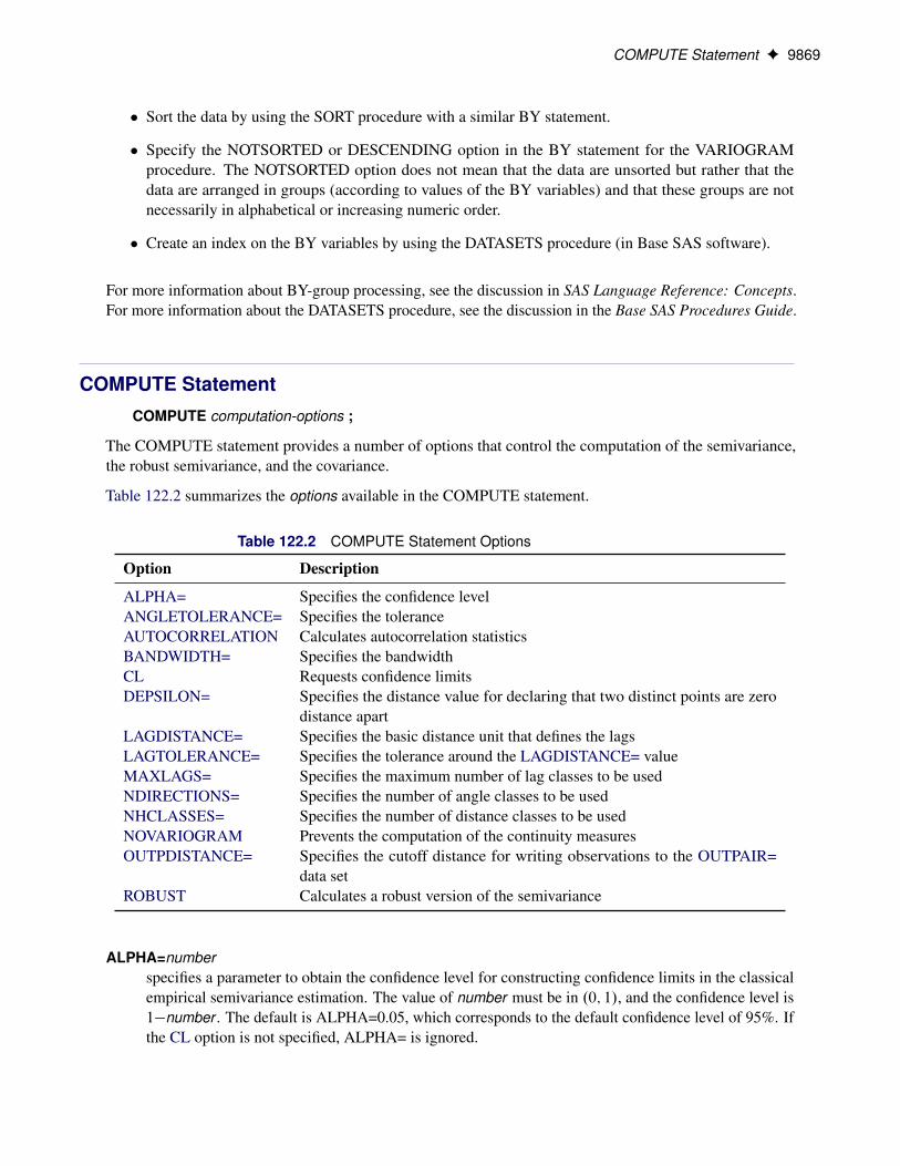
COMPUTE StatementCOMPUTE computation-options ;
The COMPUTE statement provides a number of options that control the computation of the semivariance,the robust semivariance, and the covariance.
Table 122.2 summarizes the options available in the COMPUTE statement.
Table 122.2 COMPUTE Statement Options
Option Description
ALPHA= Specifies the confidence levelANGLETOLERANCE= Specifies the toleranceAUTOCORRELATION Calculates autocorrelation statisticsBANDWIDTH= Specifies the bandwidthCL Requests confidence limitsDEPSILON= Specifies the distance value for declaring that two distinct points are zero
distance apartLAGDISTANCE= Specifies the basic distance unit that defines the lagsLAGTOLERANCE= Specifies the tolerance around the LAGDISTANCE= valueMAXLAGS= Specifies the maximum number of lag classes to be usedNDIRECTIONS= Specifies the number of angle classes to be usedNHCLASSES= Specifies the number of distance classes to be usedNOVARIOGRAM Prevents the computation of the continuity measuresOUTPDISTANCE= Specifies the cutoff distance for writing observations to the OUTPAIR=
data setROBUST Calculates a robust version of the semivariance
ALPHA=numberspecifies a parameter to obtain the confidence level for constructing confidence limits in the classicalempirical semivariance estimation. The value of number must be in .0; 1/, and the confidence level is1�number . The default is ALPHA=0.05, which corresponds to the default confidence level of 95%. Ifthe CL option is not specified, ALPHA= is ignored.

9870 F Chapter 122: The VARIOGRAM Procedure
ANGLETOLERANCE=angle-tolerance
ANGLETOL=angle-tolerance
ATOL=angle-tolerancespecifies the tolerance, in degrees, around the angles determined by the NDIRECTIONS= specification.The default is 180ı=.2nd /, where nd is the NDIRECTIONS= specification. If you do not specify theNDIRECTIONS= option or the DIRECTIONS statement, ANGLETOLERANCE= is ignored.
See the section “Theoretical and Computational Details of the Semivariogram” on page 9897 forfurther information.
AUTOCORRELATION < (autocorrelation-options) >
AUTOCORR < (autocorrelation-options) >
AUTOC < (autocorrelation-options) >specifies that autocorrelation statistics be calculated. You can further specify the followingautocorrelation-options in parentheses following the AUTOCORRELATION option.
ASSUMPTION < = assumption-options >
ASSUM < = assumption-options >specifies the type of autocorrelation assumption to use. The assumption-options can be one ofthe following:
NORMALITY | NORMAL | NORspecifies use of the normality assumption.
RANDOMIZATION | RANDOM | RANspecifies use of the randomization assumption.
The default is ASSUMPTION=NORMALITY.
STATISTICS < = (stats-options) >
STATS < = (stats-options) >specifies the autocorrelation statistics in detail. The stats-options can be one or more of thefollowing:
ALLapplies all available types of autoregression statistics.
GEARY | GEAspecifies use of the Geary’s c statistics.
MORAN | MORspecifies use of the Moran’s I statistics.
The default is STATISTICS=ALL.
WEIGHTS < = weights-options >
WEI < = weights-options >specifies the scheme used for the computation of the autocorrelation weights. You can chooseone of the following weights-options:
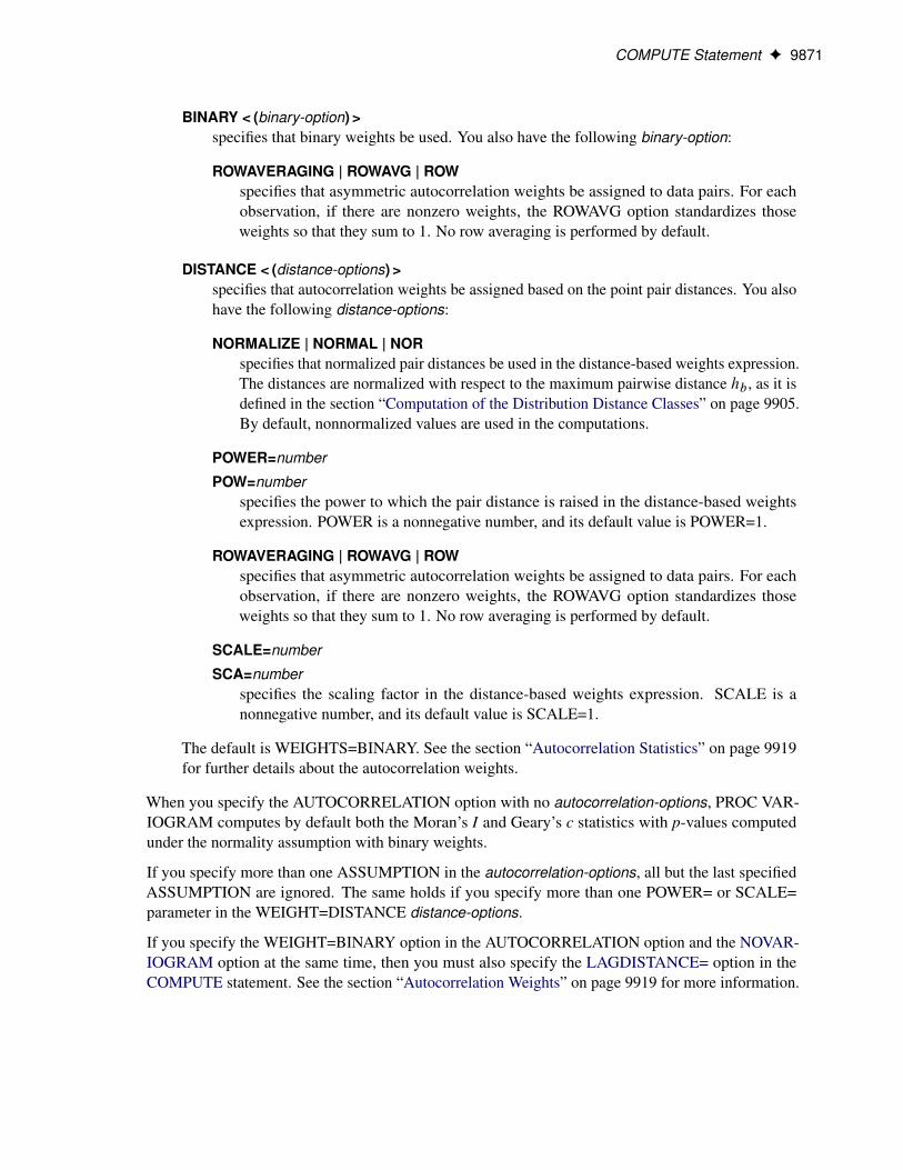
COMPUTE Statement F 9871
BINARY < (binary-option) >specifies that binary weights be used. You also have the following binary-option:
ROWAVERAGING | ROWAVG | ROWspecifies that asymmetric autocorrelation weights be assigned to data pairs. For eachobservation, if there are nonzero weights, the ROWAVG option standardizes thoseweights so that they sum to 1. No row averaging is performed by default.
DISTANCE < (distance-options) >specifies that autocorrelation weights be assigned based on the point pair distances. You alsohave the following distance-options:
NORMALIZE | NORMAL | NORspecifies that normalized pair distances be used in the distance-based weights expression.The distances are normalized with respect to the maximum pairwise distance hb , as it isdefined in the section “Computation of the Distribution Distance Classes” on page 9905.By default, nonnormalized values are used in the computations.
POWER=number
POW=numberspecifies the power to which the pair distance is raised in the distance-based weightsexpression. POWER is a nonnegative number, and its default value is POWER=1.
ROWAVERAGING | ROWAVG | ROWspecifies that asymmetric autocorrelation weights be assigned to data pairs. For eachobservation, if there are nonzero weights, the ROWAVG option standardizes thoseweights so that they sum to 1. No row averaging is performed by default.
SCALE=number
SCA=numberspecifies the scaling factor in the distance-based weights expression. SCALE is anonnegative number, and its default value is SCALE=1.
The default is WEIGHTS=BINARY. See the section “Autocorrelation Statistics” on page 9919for further details about the autocorrelation weights.
When you specify the AUTOCORRELATION option with no autocorrelation-options, PROC VAR-IOGRAM computes by default both the Moran’s I and Geary’s c statistics with p-values computedunder the normality assumption with binary weights.
If you specify more than one ASSUMPTION in the autocorrelation-options, all but the last specifiedASSUMPTION are ignored. The same holds if you specify more than one POWER= or SCALE=parameter in the WEIGHT=DISTANCE distance-options.
If you specify the WEIGHT=BINARY option in the AUTOCORRELATION option and the NOVAR-IOGRAM option at the same time, then you must also specify the LAGDISTANCE= option in theCOMPUTE statement. See the section “Autocorrelation Weights” on page 9919 for more information.

9872 F Chapter 122: The VARIOGRAM Procedure
BANDWIDTH=bandwidth-distance
BANDW=bandwidth-distancespecifies the bandwidth, or perpendicular distance cutoff for determining the angle class for a givenpair of points. The distance classes define a series of cylindrically shaped areas, while the angle classesradially cut these cylindrically shaped areas. For a given angle class .�1 � ı�1; �1 C ı�1/, as youproceed out radially, the area encompassed by this angle class becomes larger. The BANDWIDTH=option restricts this area by excluding all points with a perpendicular distance from the line � D �1that is greater than the BANDWIDTH= value. See Figure 122.23 for a visual representation of thebandwidth.
If you omit the BANDWIDTH= option, no restriction occurs. If you omit the NDIRECTIONS= optionor the DIRECTIONS statement, BANDWIDTH= is ignored.
CLrequests confidence limits for the classical semivariance estimate. The lower bound of the confidencelimits is always nonnegative, adhering to the behavior of the theoretical semivariance. You can controlthe confidence level with the ALPHA= option.
DEPSILON=distance-value
DEPS=distance-valuespecifies the distance value for declaring that two distinct points are zero distance apart. Such pairs,if they occur, cause numeric problems. If you specify DEPSILON=�", then pairs of points P1 andP2 for which the distance between them j P1P2 j< �" are excluded from the continuity measurecalculations. The default value of the DEPSILON= option is 100 times the machine precision; thisproduct is approximately 1E–10 on most computers.
LAGDISTANCE=distance-unit
LAGDIST=distance-unit
LAGD=distance-unitspecifies the basic distance unit that defines the lags. For example, a specification of LAGDISTANCE=xresults in lag distance classes that are multiples of x. For a given pair of points P1 and P2, the distancebetween them, denoted j P1P2 j, is calculated. If j P1P2 jD x, then this pair is in the first lag class. Ifj P1P2 jD 2x, then this pair is in the second lag class, and so on.
For irregularly spaced data, the pairwise distances are unlikely to fall exactly on multiples of theLAGDISTANCE= value. In this case, a distance tolerance of ıx accommodates a spread of distancesaround multiples of x (the LAGTOLERANCE= option specifies the distance tolerance). For example,if j P1P2 j is within x ˙ ıx, you would place this pair in the first lag class; if j P1P2 j is within2x ˙ ıx, you would place this pair in the second lag class; and so on.
You can experiment and determine the candidate values for the LAGDISTANCE= option by plottingthe pairwise distance histogram for different numbers of histogram classes, using the NHCLASSES=option.
A LAGDISTANCE= value is required for the semivariance and the autocorrelation computations.However, when you specify the NOVARIOGRAM option without the AUTOCORRELATION option,you need not specify the LAGDISTANCE= option.
See the section “Theoretical and Computational Details of the Semivariogram” on page 9897 for moreinformation.

COMPUTE Statement F 9873
LAGTOLERANCE=tolerance-number
LAGTOL=tolerance-number
LAGT=tolerance-numberspecifies the tolerance around the LAGDISTANCE= value for grouping distance pairs into lag classes.See the description of the LAGDISTANCE= option for information about the use of the LAGTOLER-ANCE= option, and the section “Theoretical and Computational Details of the Semivariogram” onpage 9897 for more details.
If you omit the LAGTOLERANCE= option, a default value of 12
times the LAGDISTANCE= value isused.
MAXLAGS=number-of-lags
MAXLAG=number-of-lags
MAXL=number-of-lagsspecifies the maximum number of lag classes to be used in constructing the continuity measures inaddition to a zero lag class; see also the section “Distance Classification” on page 9903. This optionexcludes any pair of points P1 and P2 for which the distance between them, j P1P2 j, exceeds theMAXLAGS= value times the LAGDISTANCE= value.
You can determine candidate values for the MAXLAGS= option by plotting or displaying the OUT-DISTANCE= data set.
A MAXLAGS= value is required unless you specify the NOVARIOGRAM option.
NDIRECTIONS=number-of-directions
NDIR=number-of-directions
ND=number-of-directionsspecifies the number of angle classes to use in computing the continuity measures. This option is usefulwhen there is potential anisotropy in the spatial continuity measures. Anisotropy is a field property inwhich the characterization of spatial continuity depends on the data pair orientation (or angle betweenthe N–S direction and the axis defined by the data pair). Isotropy is the absence of this effect; that is,the description of spatial continuity depends only on the distance between the points, not the angle.
The angle classes formed from the NDIRECTIONS= option start from N–S and proceed clockwise.For example, NDIRECTIONS=3 produces three angle classes. In terms of compass points, theseclasses are centered at 0ı (or its reciprocal, 180ı), 60ı (or its reciprocal, 240ı), and 120ı (or itsreciprocal, 300ı). For irregularly spaced data, the angles between pairs are unlikely to fall exactly inthese directions, so an angle tolerance of ı� is used (the ANGLETOLERANCE= option specifies theangle tolerance). If NDIRECTIONS=nd , the base angle is � D 180ı=nd , and the angle classes are
.k� � ı�; k� C ı�/ k D 0; : : : ; nd � 1
If you omit the NDIRECTIONS= option, no angles are formed. This is the omnidirectional case wherethe spatial continuity measures are assumed to be isotropic.
The NDIRECTIONS= option is useful for exploring possible anisotropy. The DIRECTIONS statement,described in the section “DIRECTIONS Statement” on page 9875, provides greater control over theangle classes.
See the section “Theoretical and Computational Details of the Semivariogram” on page 9897 for moreinformation.

9874 F Chapter 122: The VARIOGRAM Procedure
NHCLASSES=number-of-histogram-classesNHCLASS=number-of-histogram-classesNHC=number-of-histogram-classes
specifies the number of distance classes to consider in the spatial domain in the exploratory stageof the empirical semivariogram computation. The actual number of classes is one more than theNHCLASSES= value, since a special lag zero class is also computed. The NHCLASSES= optionis used to produce the distance intervals table, the histogram of pairwise distances, and the OUT-DISTANCE= data set. See the OUTDISTANCE= option, the section “OUTDIST=SAS-data-set”on page 9925, and the section “Theoretical and Computational Details of the Semivariogram” onpage 9897 for more information.
The default value is NHCLASSES=10.
NOVARIOGRAMprevents the computation of the continuity measures. This option is useful for preliminary analysis, orwhen you require only the OUTDISTANCE= or OUTPAIR= data sets.
OUTPDISTANCE=distance-limitOUTPDIST=distance-limitOUTPD=distance-limit
specifies the cutoff distance for writing observations to the OUTPAIR= data set. If you specifyOUTPDISTANCE=dmax , the distance j P1P2 j between each pair of points P1 and P2 is checkedagainst dmax . If j P1P2 j> dmax , the observation for this pair is not written to the OUTPAIR= dataset. If you omit the OUTPDISTANCE= option, all distinct pairs are written. This option is ignored ifyou omit the OUTPAIR= data set.
ROBUSTrequests that a robust version of the semivariance be calculated in addition to the classical semivariance.
COORDINATES StatementCOORDINATES coordinate-variables ;
The following two options give the names of the variables in the DATA= data set that contains the values ofthe x and y coordinates of the data.
Only one COORDINATES statement is allowed, and it is applied to all the analysis variables. In other words,it is assumed that all the VAR variables have the same x and y coordinates.
XCOORD=(variable-name)XC=(variable-name)X=(variable-name)
gives the name of the variable that contains the x coordinate of the data in the DATA= data set.
YCOORD=(variable-name)YC=(variable-name)Y=(variable-name)
gives the name of the variable that contains the y coordinate of the data in the DATA= data set.
DIRECTIONS Statement F 9875
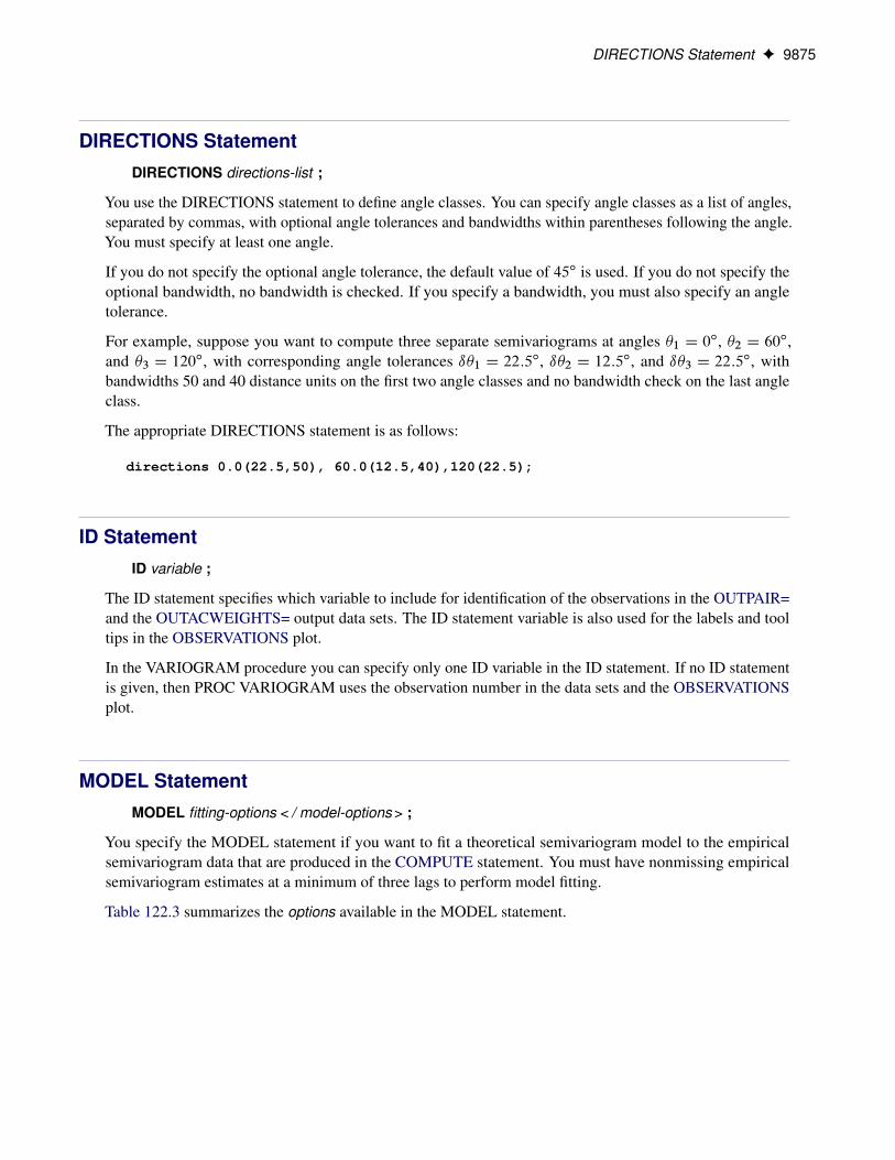
DIRECTIONS StatementDIRECTIONS directions-list ;
You use the DIRECTIONS statement to define angle classes. You can specify angle classes as a list of angles,separated by commas, with optional angle tolerances and bandwidths within parentheses following the angle.You must specify at least one angle.
If you do not specify the optional angle tolerance, the default value of 45ı is used. If you do not specify theoptional bandwidth, no bandwidth is checked. If you specify a bandwidth, you must also specify an angletolerance.
For example, suppose you want to compute three separate semivariograms at angles �1 D 0ı, �2 D 60ı,and �3 D 120ı, with corresponding angle tolerances ı�1 D 22:5ı, ı�2 D 12:5ı, and ı�3 D 22:5ı, withbandwidths 50 and 40 distance units on the first two angle classes and no bandwidth check on the last angleclass.
The appropriate DIRECTIONS statement is as follows:
directions 0.0(22.5,50), 60.0(12.5,40),120(22.5);
ID StatementID variable ;
The ID statement specifies which variable to include for identification of the observations in the OUTPAIR=and the OUTACWEIGHTS= output data sets. The ID statement variable is also used for the labels and tooltips in the OBSERVATIONS plot.
In the VARIOGRAM procedure you can specify only one ID variable in the ID statement. If no ID statementis given, then PROC VARIOGRAM uses the observation number in the data sets and the OBSERVATIONSplot.
MODEL StatementMODEL fitting-options < / model-options > ;
You specify the MODEL statement if you want to fit a theoretical semivariogram model to the empiricalsemivariogram data that are produced in the COMPUTE statement. You must have nonmissing empiricalsemivariogram estimates at a minimum of three lags to perform model fitting.
Table 122.3 summarizes the options available in the MODEL statement.

9876 F Chapter 122: The VARIOGRAM Procedure
Table 122.3 MODEL Statement Options
Option Description
Fitting OptionsALPHA= Specifies confidence levelCHOOSE= Ranks the fitted models and chooses the optimally fit modelCL Constructs a t-type confidence intervalEQUIVTOL= Specifies a positive upper value toleranceFIT= Specifies which type of empirical semivariogram to fitFORM= Specifies the functional form (type) of the semivariogram modelMDATA= Specifies the input data setMETHOD= Fits a theoretical model to the empirical semivarianceNEPSILON= Adds a minimal nugget effectNUGGET= Specifies the nugget effectRANGE= Specifies the range parameterRANGELAG= Uses consecutive nonmissing empirical semivariance lags to fit modelRANKEPS= Specifies the minimum threshold to compare fit qualitySCALE= Specifies the scale parameter in semivariogram modelsSMOOTH= Specifies the positive smoothness parameter �
Model OptionsCOVB Requests the covariance matrixCORRB Requests the approximate correlation matrixDETAILS Produces different levels of outputGRADIENT Displays the gradient of the objective functionMTOGTOL= Specifies a threshold value for the smoothness parameterNOFIT Suppresses the model fitting processNOITPRINT Suppresses the display of the iteration history table
You can choose to perform a fully automated fitting or to fit one model with specific forms. In the first caseyou simply specify a list of forms or no forms at all. All suitable combinations are tested, and the result is themodel that produces the best fit according to specified criteria. In the second case you specify one theoreticalsemivariogram model, and you have more control over its parameters for the fitting process.
Furthermore, you can specify a theoretical semivariogram model in two ways:
� You explicitly specify the FORM option and any of the options SCALE, RANGE, and NUGGET inthe MODEL statement.
� You can specify an MDATA= data set. This data set contains variables that correspond to the FORMoption and to any of the options SCALE, RANGE, NUGGET, and SMOOTH. You can also use anMDATA= data set to request a fully automated fitting.
The two methods are exclusive; either you specify all parameters explicitly, or they all are read from theMDATA= data set.
MODEL Statement F 9877
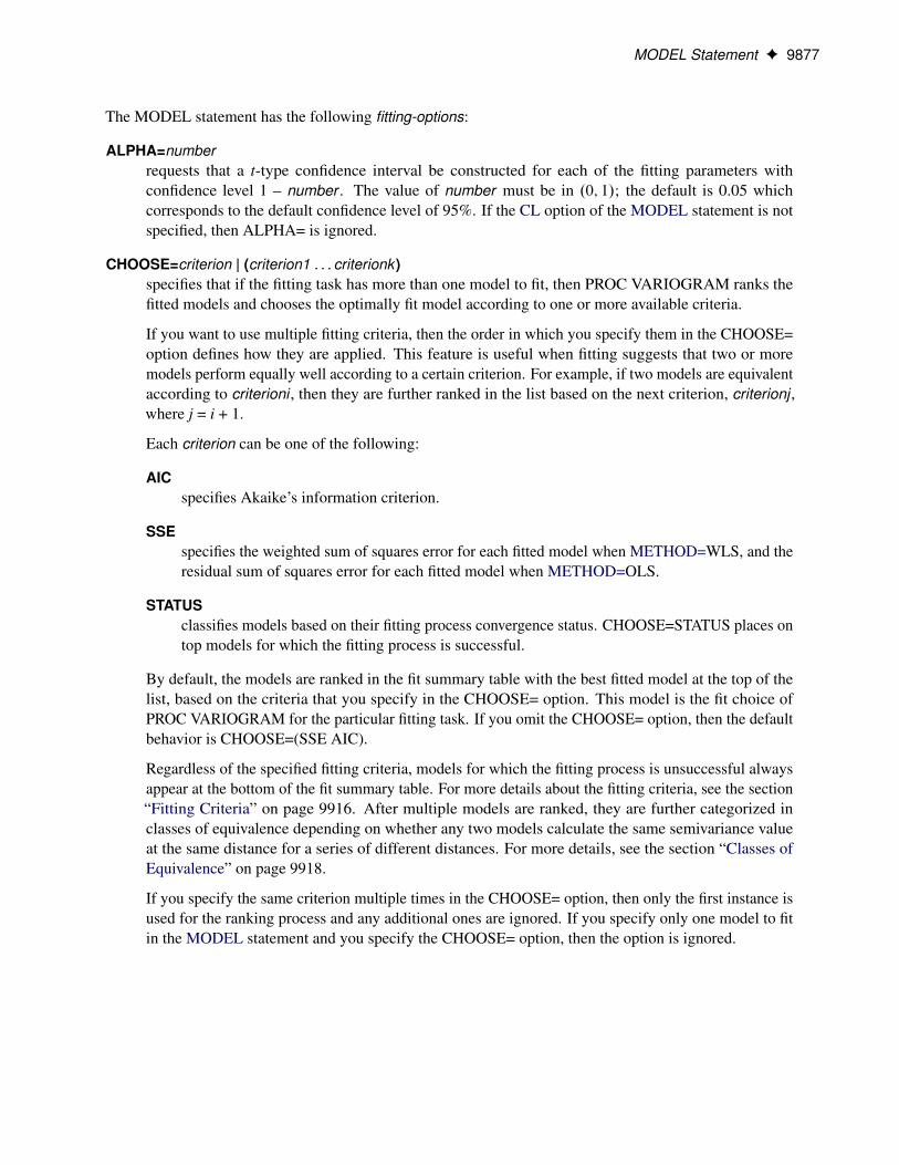
The MODEL statement has the following fitting-options:
ALPHA=numberrequests that a t-type confidence interval be constructed for each of the fitting parameters withconfidence level 1 – number . The value of number must be in .0; 1/; the default is 0.05 whichcorresponds to the default confidence level of 95%. If the CL option of the MODEL statement is notspecified, then ALPHA= is ignored.
CHOOSE=criterion | (criterion1 . . . criterionk )specifies that if the fitting task has more than one model to fit, then PROC VARIOGRAM ranks thefitted models and chooses the optimally fit model according to one or more available criteria.
If you want to use multiple fitting criteria, then the order in which you specify them in the CHOOSE=option defines how they are applied. This feature is useful when fitting suggests that two or moremodels perform equally well according to a certain criterion. For example, if two models are equivalentaccording to criterioni , then they are further ranked in the list based on the next criterion, criterionj ,where j = i + 1.
Each criterion can be one of the following:
AICspecifies Akaike’s information criterion.
SSEspecifies the weighted sum of squares error for each fitted model when METHOD=WLS, and theresidual sum of squares error for each fitted model when METHOD=OLS.
STATUSclassifies models based on their fitting process convergence status. CHOOSE=STATUS places ontop models for which the fitting process is successful.
By default, the models are ranked in the fit summary table with the best fitted model at the top of thelist, based on the criteria that you specify in the CHOOSE= option. This model is the fit choice ofPROC VARIOGRAM for the particular fitting task. If you omit the CHOOSE= option, then the defaultbehavior is CHOOSE=(SSE AIC).
Regardless of the specified fitting criteria, models for which the fitting process is unsuccessful alwaysappear at the bottom of the fit summary table. For more details about the fitting criteria, see the section“Fitting Criteria” on page 9916. After multiple models are ranked, they are further categorized inclasses of equivalence depending on whether any two models calculate the same semivariance valueat the same distance for a series of different distances. For more details, see the section “Classes ofEquivalence” on page 9918.
If you specify the same criterion multiple times in the CHOOSE= option, then only the first instance isused for the ranking process and any additional ones are ignored. If you specify only one model to fitin the MODEL statement and you specify the CHOOSE= option, then the option is ignored.

9878 F Chapter 122: The VARIOGRAM Procedure
CLrequests that t-type confidence limits be constructed for each of the fitting parameters estimates. Theconfidence level is 0.95 by default; this can be changed with the ALPHA= option of the MODELstatement.
EQUIVTOL=etol-value
ETOL=etol-valuespecifies a positive upper value tolerance to use when categorizing multiple models in classes ofequivalence. For this categorization, the VARIOGRAM procedure computes the sum of absolutedifferences of semivariances for pairs of consecutively ranked models. If the sum is lower than theEQUIVTOL= value for any such model pair, then these two models are deemed to be equivalent. Asa result, the EQUIVTOL= option can affect the number and size of classes of equivalence in the fitsummary table. Smaller values of the EQUIVTOL= parameter result in a more strict model comparisonand can lead to a higher number of classes of equivalence. For more details, see the section “Classes ofEquivalence” on page 9918.
The default value for the EQUIVTOL= parameter is 10�3. The EQUIVTOL= option applies when youfit multiple models with the FORM=AUTO option of the MODEL statement; otherwise, it is ignored.
The EQUIVTOL= option is independent of the ranking results from the RANKEPS= option of theMODEL statement. This means that you could possibly have models listed but not ranked in the fitsummary table, and still have equivalence classes assigned according to the order in which the modelsappear in the table.
FIT=fit-type-optionsspecifies which type of empirical semivariogram to fit. You can choose between the following fit-type-options:
CLASSICAL
CLAfits a model for the classical empirical semivariance.
ROBUST
ROBfits a model for the robust empirical semivariance. This option can be used only when theROBUST option is specified in the COMPUTE statement.
The default value is FIT=CLASSICAL.
FORM=form | (form1, . . . , formk ) | AUTO (auto-options)specifies the functional form (type) of the semivariogram model. The supported structures are two-parameter models that use the sill and range as parameters. The Matérn model is an exception thatmakes use of a third smoothing parameter �.
The FORM= option is required when you specify the MODEL statement. You can perform fittingof a theoretical semivariogram model either explicitly or in an automated manner. For the explicitspecification you specify suitable model forms in the FORM= option. For an automated fit you specifythe FORM=AUTO option which has the AUTO(MLIST=) and AUTO(NEST=) suboptions. You canread more details in the following two subsections.

MODEL Statement F 9879
Explicit Model Specification
You can explicitly specify a theoretical semivariogram model to fit by using any combination of one, two,or three forms. Use the syntax with the single form to specify a non-nested model. Use the syntax with kstructures formi , i = 1, . . . , k, to specify up to three nested structures (k � 3) in a semivariogram model. Eachof the forms can be any of the following:
CUBIC | EXPONENTIAL | GAUSSIAN | MATERN |
PENTASPHERICAL | POWER | SINEHOLEEFFECT | SPHERICAL
CUB | EXP | GAU | MAT | PEN | POW | SHE | SPHspecify a form.
All of these forms are presented in more detail in the section “Theoretical Semivariogram Models” onpage 9892. In addition, you can optionally specify a nugget effect for your model with the NUGGET optionin the MODEL statement.
For example, the syntax
FORM=GAU
specifies a model with a single Gaussian structure. Also, the syntax
FORM=(EXP,SHE,MAT)
specifies a nested model with an exponential, a sine hole effect, and a Matérn structure. Finally
FORM=(EXP,EXP)
specifies a nested model with two structures both of which are exponential.
NOTE: In the documentation, models are named either by using their full names or by using the first threeletters of their structures. Also, the names of different structures in a nested model are separated by a hyphen(-). According to this convention, the previous examples illustrate how to specify a GAU, an EXP-SHE-MAT,and an EXP-EXP model, respectively, with the FORM= option.
When you explicitly specify the types of structures, you can fix parameter values or ask PROC VARIOGRAMto select default initial values for the forms parameters by using the SCALE, RANGE, NUGGET, andSMOOTH options. You can set your own, non-default initial parameter values by using the PARMS statementin combination with an explicitly specified semivariogram model in the MODEL statement.
Automated Model Selection
Use the FORM=AUTO option to request the highest level of automation in the best fit selection of theparameters. If you specify FORM=AUTO, any of the SCALE, RANGE, or SMOOTH options that are alsospecified are ignored. When you specify the FORM=AUTO option, you cannot specify the PARMS statementfor the corresponding MODEL statement. As a result, when you use the FORM=AUTO option, you cannotfix any of the model parameters and PROC VARIOGRAM sets initial values for them.
The AUTO option has the following auto-options:
MLIST=mform | (mform1, . . . , mformp)specifies one or more different model forms to use in combinations during the model fitting process. Ifyou omit the MLIST= suboption, then combinations are made among all available model types. Themform can be any of the following eight forms:

9880 F Chapter 122: The VARIOGRAM Procedure
CUBIC | EXPONENTIAL | GAUSSIAN | MATERN |
PENTASPHERICAL | POWER | SINEHOLEEFFECT | SPHERICAL
CUB | EXP | GAU | MAT | PEN | POW | SHE | SPHspecify a form.
If you use more than one mform, then each mformi, i = 1, . . . , p must be different from the others in thegroup of p � 8 forms that you specify.
NEST=nest-listspecifies the number of nested structures to use for the fitting. You can choose between the followingto specify the nest-list:
n a single value
m TO n a sequence in which m equals the starting value and n equals the ending value
For example,
NEST=1
produces the best fit with one single model among all model types specified in the MLIST= suboption.Also,
NEST=2 TO 3
produces the best fit among all combinations of the model types specified in the MLIST= suboptionthat result in nested models with two or three structures. The combinations that are tested includerepetitions. Hence, if you specify, for example,
MODEL FORM=AUTO(MLIST=(EXP,SPH) NEST=1 TO 2)
then the different models that are tested are equivalent to the specifications FORM=EXP, FORM=SPH,FORM=(EXP,EXP), FORM=(EXP,SPH), FORM=(SPH,SPH) and FORM=(SPH,EXP). NOTE: Themodels EXP-SPH and SPH-EXP are taken as two separate models. Although they are mathematicallyequivalent (see the section “Nested Models” on page 9897), PROC VARIOGRAM assigns differentinitial values to the model structures in each case, which can lead to different fitting results. (See thesection “Example 122.1: Aspects of Semivariogram Model Fitting” on page 9931.)
If you omit the NEST suboption, then by default PROC VARIOGRAM searches for the best fit withup to three nested structures in a model. The default behavior is equivalent to
NEST=1 TO 3

MODEL Statement F 9881
In the VARIOGRAM procedure you can use a maximum of three nested structures to fit an empiricalsemivariogram; that is, n � 3.
You can use the AUTO value for the form in the MDATA= data set, and also in the FORM= option. However,in the former case the automation functionality is limited compared to the latter case and the auto-options ofthe FORM=AUTO option. In particular, when you specify the form to be AUTO in the MDATA= data set,then PROC VARIOGRAM follows only the default behavior and searches among all available forms for thebest fit with up to three nested structures in a model.
MDATA=SAS-data-setspecifies the input data set that contains parameter values for the covariance or semivariogram model.The MDATA= data set must contain a variable named FORM, and it can optionally include any of thevariables SCALE, RANGE, NUGGET, and SMOOTH.
The FORM variable must be a character variable. It accepts only the AUTO value or the form valuesthat can be specified in the FORM= option in the MODEL statement. The RANGE, SCALE, NUGGET,and SMOOTH variables must be numeric or missing.
The number of observations present in the MDATA= data set corresponds to the level of nesting of thesemivariogram model. Each observation line describes a structure of the model you submit for fitting.
If you specify the AUTO value for the FORM variable in an observation, then you cannot specifyadditional nested structures in the same data set, and any parameters you specify in the same structureare ignored. In that case, PROC VARIOGRAM performs a crude automated search among all availableforms to obtain the best fit with up to three nested structures in a model. You can refine this type ofsearch with additional suboptions when you perform it with the FORM=AUTO option instead of theMDATA= option in the MODEL statement.
When you have a nested model, you might want to specify parameter values for only some of thenested structures. In this case, you must specify the corresponding parameter values for the remainingmodel structures as missing values.
For example, you can use the following DATA step to specify a non-nested model that uses a sphericalcovariance within an MDATA= data set:
data md1;input scale range form $;datalines;
25 10 SPH;
Then, you can use the md1 data in the MODEL statement of PROC VARIOGRAM as shown in thefollowing statements:
proc variogram data=...;compute ...;model mdata=md1;
run;
This is equivalent to the following explicit specification of the semivariance model parameters:

9882 F Chapter 122: The VARIOGRAM Procedure
proc variogram data=...;compute ...;model form=sph scale=25 range=10;
run;
The following data set md2 is an example of a nested model:
data md2;input form $ scale range nugget smooth;datalines;
SPH 20 8 5 .MAT 12 3 5 0.7GAU . 1 5 .;
This specification is equivalent to the following explicit specification of the semivariance modelparameters:
proc variogram data=...;compute ....;model form=(sph,mat,gau)
scale=(20,12,.) range=(8,3,1) smooth=0.7 nugget=5;run;
Use the SMOOTH variable column in the MDATA= data set to specify the smoothing parameter �in the Matérn semivariogram models. The SMOOTH variable values must be positive and no greaterthan 1,000,000. PROC VARIOGRAM sets this upper limit for numerical and performance reasons.In any case, if the fitting process leads the smoothness value to exceed the default threshold value10,000, then the VARIOGRAM procedure converts the Matérn form into a Gaussian form and repeatsthe model fitting. To adjust the switching threshold value, you can use the MTOGTOL= option in theMODEL statement.
If you specify a SMOOTH column in the MDATA= data set, then its elements are ignored except forthe rows in which the corresponding FORM is Matérn.
The NUGGET variable value is the same for all nested structures. This is the way to specify a nuggeteffect in the MDATA= data set. If you specify more than one nugget value for different structures, thenthe last nugget value specified is used.
METHOD=method-optionsmust be specified in the MODEL statement to fit a theoretical model to the empirical semivariance.The METHOD option has the following suboptions:
OLSspecifies that ordinary least squares be used for the fitting.
WLSspecifies that weighted least squares be used for the fitting.
The default is METHOD=WLS.

MODEL Statement F 9883
NEPSILON=min-nugget-factor
NEPS=min-nugget-factorspecifies that a minimal nugget effect be added to the theoretical semivariance in the unlikely occasionthat the theoretical semivariance becomes zero during fitting with weighted least squares. As explainedin the section “Theoretical and Computational Details of the Semivariogram” on page 9897, thetheoretical semivariance is always positive for any distance larger than zero. If a conflicting situationemerges as a result of numerical fitting issues, then the NEPSILON= option can help you alleviate theproblem by adding a minimal variance at the distance lag where the issue is encountered. For moredetails, see the section “Parameter Initialization” on page 9913.
If you omit the NEPSILON= option, then PROC VARIOGRAM sets a default value of 10�6. Ifa minimal nugget effect is used, its value is case-specific and is based on the min-nugget-factor .Specifically, its value is defined as min-nugget-factor times the sample variance of the input data set,or as min-nugget-factor when the sample variance is equal to zero.
NUGGET=numberspecifies the nugget effect for the model. The nugget effect is due to a discontinuity in the semivari-ogram as determined by plotting the sample semivariogram; see “Theoretical Semivariogram Models”on page 9892 for more details. The NUGGET= parameter is a nonnegative number. If you specify anonmissing value, then it is used as a fixed parameter in the fitting process.
PROC VARIOGRAM assigns a default initial value for the nugget effect in the following cases:
� if you specify a missing value.
� if you omit the NUGGET= option and you do not specify an associated PARMS statement withinitial values for the nugget.
The NUGGET= option is incompatible with the specification of the PARMS statement for the corre-sponding MODEL statement.
RANGE=range | (range1, . . . , rangek )specifies the range parameter in semivariogram models. The RANGE= option is optional. However,if you specify the RANGE= option, then you must provide range values for all structures that youhave specified explicitly in the FORM= option. All nonmissing range values are considered as fixedparameters. PROC VARIOGRAM assigns a default initial value to any of the model structures forwhich you specify a missing range value. PROC VARIOGRAM assigns default initial values to allmodel structures if you omit the RANGE= option, unless you specify an associated PARMS statementand initial values for the range in it.
The range parameter is a positive number, has the units of distance, and is related to the correlationscale of the underlying spatial process.
NOTE: If you specify this parameter for a power model, then it does not correspond to a range. Forpower models, the parameter you specify in the RANGE option is a dimensionless power exponentwhose value must range within [0,2) so that the power model is a valid semivariance function.
The RANGE= option is ignored when you specify the FORM=AUTO option. The RANGE= option isincompatible with the specification of the PARMS statement for the corresponding MODEL statement.
9884 F Chapter 122: The VARIOGRAM Procedure
RANGELAG=rlag-list
RLAG=rlag-listspecifies that you prefer to use the range of consecutive nonmissing empirical semivariance lags in therlag-list for the semivariogram fitting process, instead of using all MAXLAGS+1 lag classes by default.You can specify rlag-list in either of the following forms:
k a single value that designates the width of the selected lag range by starting atlag zero. You must use at least three lags to perform model fitting, so you canspecify k within [3, : : : , MAXLAGS+1].
m TO n a sequence in which m equals the starting lag and n equals the ending lag. Theparameters m and n must be nonnegative integer numbers to designate lag classesbetween zero and MAXLAGS. Use at least three lags for model fitting; hence itholds that n �m � 2.
The following two brief examples exhibit the use of the RANGELAG option. These examples assumethat you have set the MAXLAGS= option to 9 or higher to indicate nonmissing empirical semivarianceestimates at 10 lags or more.
In the first example,
RANGELAG=8
uses the empirical semivariance in the first eight lags to fit a theoretical model. Hence, RANGELAG=8uses only the lag classes zero to seven. This approach enables you to account only for the correlationbehavior described by the first k empirical semivariogram lag classes.
In the second example,
RANGELAG=2 TO 9
specifies that the empirical semivariance values at lag classes zero, one, and after lag class nine areexcluded from the model fitting process.
RANKEPS=reps-value
REPS=reps-valuespecifies the minimum threshold to compare fit quality of two models for a specific criterion. Beyondthis threshold the criterion values become insensitive to comparison. In particular, when you fit multiplemodels, PROC VARIOGRAM computes for each one the value of the fitting criterion specified inthe CHOOSE= option of the MODEL statement. These values are examined in pairs at the sortingstage. If the difference of a given pair exceeds the reps-value, then the sort order of the correspondingmodels is reversed; otherwise, the two models retain their relative order in the rankings. Hence, theRANKEPS= option can affect model ranking in the fit summary table.
The default value for the RANKEPS= parameter is 10�6 and accounts for the default optimizationconvergence tolerance at the fitting stage prior to model ranking. The convergence tolerance itselflimits the accuracy that you can use to compare two models under a given criterion. As a result, smallervalues of the RANKEPS= parameter might not lead to a sensible and more strict model comparisonbecause for a smaller reps-value, ranking could depend on digits beyond the accuracy limit.
MODEL Statement F 9885
In the opposite end, if the specified reps-value turns out to be large compared to the criterion valuedifferences, then it can make the sorting process insensitive to the specified sorting criterion. When thishappens, the fit summary table ranking reflects only the order in which different models are examinedin the procedure flow. You can tell whether the criterion is bypassed; if it is, then one or more values ofthe specified criterion might not appear to be sorted in the fit summary table.
The RANKEPS= parameter must be a positive number. The RANKEPS= option applies when you fitmultiple models with the FORM=AUTO option of the MODEL statement; otherwise, it is ignored.
SCALE=scale | (scale1, . . . , scalek )specifies the scale parameter in semivariogram models. The SCALE= option is optional. However,if you specify the SCALE= option, then you must provide sill values for all structures that youhave specified explicitly in the FORM= option. All nonmissing scale values are considered as fixedparameters. PROC VARIOGRAM assigns a default initial value to any of the model structures forwhich you specify a missing scale value. PROC VARIOGRAM assigns default initial values to allmodel structures if you omit the SCALE= option, unless you specify an associated PARMS statementwith initial values for scale.
The scale parameter is a positive number. It has the same units as the variance of the variable inthe VAR statement. The scale of each structure in a semivariogram model represents the variancecontribution of the structure to the total model variance.
In power models the SCALE= parameter does not correspond to a sill because the power model has nosill. Instead, PROC VARIOGRAM uses the SCALE= option to designate the slope (or scaling factor)in power model forms. The power model slope has the same variance units as the variable in the VARstatement.
The SCALE= option is ignored when you specify the FORM=AUTO option. The SCALE= option isincompatible with the specification of the PARMS statement for the corresponding MODEL statement.
SMOOTH=smooth | (smooth1, . . . , smoothm)specifies the positive smoothness parameter � in the Matérn type of semivariance structures. Thespecial case � D 0:5 is equivalent to the exponential model, whereas the theoretical limit � ! 1gives the Gaussian model.
The SMOOTH= option is optional. When you specify an explicit model in the FORM= option with mMatérn structures, you can provide up to m smoothness values. You can specify a value for smoothi ,i D 1; : : : ; m that is positive and no greater than 1,000,000. PROC VARIOGRAM sets this upperlimit for the SMOOTH= option values for numerical and performance reasons. In any case, if thefitting process leads the smoothness value to exceed the default threshold value 10,000, then theVARIOGRAM procedure converts the Matérn form into a Gaussian form and repeats the model fitting.To adjust the switching threshold value, you can use the MTOGTOL= option in the MODEL statement.
If you specify fewer than m values, then the remaining Matérn structures have their smoothnessparameters initialized to missing values. If you specify more than m values, then values in excess areignored.
All nonmissing smoothness values are considered as fixed parameters of the corresponding Matérnstructures. PROC VARIOGRAM assigns a default initial value to any of the model Matérn structures,if any, for which you specify a missing smoothness value. PROC VARIOGRAM assigns defaultinitial values to all model Matérn structures if you omit the SMOOTH= option, unless you specify anassociated PARMS statement and initial values for smoothness in it.

9886 F Chapter 122: The VARIOGRAM Procedure
The SMOOTH= option is ignored when you specify the FORM=AUTO option. The SMOOTH=option is incompatible with the specification of the PARMS statement for the corresponding MODELstatement.
In addition to the fitting-options, you can specify the following model-options after a slash (/) in the MODELstatement.
COVBrequests the approximate covariance matrix for the parameter estimates of the model fitting. TheCOVB option is ignored when you also specify the DETAILS=ALL option.
When you specify an explicit model with the FORM= option in the MODEL statement, the COVBoption produces the requested approximate covariance matrix. When you specify the FORM=AUTOoption in the MODEL statement, by default the COVB option produces output only for the selectedmodel, where the choice is based on the criteria that you specify in the CHOOSE= option of theMODEL statement. If you specify the DETAILS option in addition to FORM=AUTO in the MODELstatement, then the COVB option produces output for each one of the fitted models.
CORRBrequests the approximate correlation matrix for the parameter estimates of the model fitting. TheCORRB option is ignored when you also specify the DETAILS=ALL option.
When you specify an explicit model with the FORM= option in the MODEL statement, the CORRBoption produces the requested approximate correlation matrix. When you specify the FORM=AUTOoption in the MODEL statement, by default the CORRB option produces output only for the selectedmodel, where the choice is based on the criteria that you specify in the CHOOSE= option of theMODEL statement. If you specify the DETAILS option in addition to FORM=AUTO in the MODELstatement, then the CORRB option produces output for each one of the fitted models.
DETAILS < = detail-level >requests different levels of output to be produced during the fitting process. You can specify any of thefollowing detail-level arguments:
MODspecifies that the default output for all candidate models be produced when the FORM=AUTOoption is specified in the MODEL statement. If you fit only one explicit model, then theDETAILS=MOD option has no effect and is ignored.
ITRrequests that a complete iteration history be produced in addition to the default output. The outputfor DETAILS=ITR includes the current values of the parameter estimates, their gradients, andadditional optimization statistics.
ALLrequests the most detailed level of output when fitting a model. Specifically, except for the defaultoutput, the DETAILS=ALL option produces optimization statistics in addition to the combinedoutput of the DETAILS=ITR, COVB, and CORRB options.
When you fit multiple models with the FORM=AUTO option in the MODEL statement, only theselected model default output is produced. The model selection is based on the criteria that you specifyin the CHOOSE= option of the MODEL statement. With the DETAILS option you can produce ODStables with information about the fitting process of all the models that you fit. Moreover, you canproduce output at different levels of detail that you can specify with the detail-level argument.

PARMS Statement F 9887
Omitting the DETAILS option or specifying the DETAILS option without any argument is equivalentto specifying DETAILS=MOD.
GRADIENTdisplays the gradient of the objective function with respect to the parameter estimates in the “ParameterEstimates” table.
MTOGTOL=numberMTOL=number
specifies a threshold value for the smoothness parameter of the Matérn form. Above this threshold, aMatérn form in a model switches to the Gaussian form. The number value must be positive and nogreater than 1,000,000, which is the smoothness upper bound set by the VARIOGRAM procedure.
By default, if the fitting process progressively increases the Matérn smoothness parameter � withoutconverging to a smoothness estimate, then PROC VARIOGRAM converts the Matérn form into aGaussian form when smoothness exceeds the default value 10,000. If you specify the number value tobe greater than the 1,000,000 boundary value, then it is ignored and reset to the default threshold value.For more details about the Matérn-to-Gaussian form conversion, see the section “Fitting with MatérnForms” on page 9918.
NOFITsuppresses the model fitting process.
NOITPRINTsuppresses the display of the iteration history table when you have also specified the DETAILS=ITR orDETAILS=ALL option in the MODEL statement. Otherwise, the NOITPRINT option is ignored.
PARMS StatementPARMS (value-list). . . < / options > ;
The PARMS statement specifies initial values for the semivariance parameters of a single specified model inthe MODEL statement. Alternatively, the PARMS statement can request a grid search over several values ofthese parameters. You must specify the values by starting with the nugget effect parameter. You continue inthe order in which semivariogram forms are specified in the FORM= option of the MODEL statement byspecifying for each structure the values for its scale, range, and any other parameters as applicable.
The PARMS statement is optional and must follow the associated MODEL statement.
The value-list specification can take any of several forms:
m a single value
m1; m2; : : : ; mn several values
m to n a sequence in which m equals the starting value, n equals the ending value, and theincrement equals 1
m to n by i a sequence in which m equals the starting value, n equals the ending value, and theincrement equals i
m1; m2 to m3 mixed values and sequences

9888 F Chapter 122: The VARIOGRAM Procedure
You can use the PARMS statement to input fixed values for parameters and also initial values that you wantto optimize.
Suppose that you want to fit a semivariogram model with a Matérn component of scale 3, range 20, smoothingparameter 4.5, and an exponential component of unspecified scale and range 15. Assume that you also wantto fix all the specified parameter values for the optimization. Including the nugget effect, you have a modelwith six parameters.
In terms of the PARMS statement, your specifications mean that you have initial values for the second, third,fourth, and sixth parameter in the parameter list. Also, the same specifications imply that you provide noinitial values for the first parameter (which corresponds to the nugget effect) and the fifth parameter (whichcorresponds to the exponential model scale). For these parameters you prefer that PROC VARIOGRAMselects initial values, instead. Since you must specify values for all model parameters in the PARMSstatement, you simply specify missing values for the first and fifth parameter. This is the way to request thatPROC VARIOGRAM assigns default initial values to parameters. The SAS statements to implement thesespecifications are as follows:
proc variogram data=FirstData;< other VARIOGRAM statements >model form=(mat,exp);parms (.) (3) (20) (4.5) (.) (15) / hold=(2 to 4,6);
run;
NOTE: The preceding statements are equivalent to the following ones in which the PARMS statement isomitted:
proc variogram data=FirstData;< other VARIOGRAM statements >model form=(mat,exp) scale=(3,.) range(20,15) smooth=4.5;
run;
This example might suggest that you can always use either the PARMS or the MODEL statement to specifythe same fitting parameters in the VARIOGRAM procedure. However, the PARMS statement gives you moreflexibility in two ways:
� You can set non-default initial parameter values by using the PARMS statement, whereas in theMODEL statement you can request default initial values only by setting parameters to missing values.For this reason the PARMS statement cannot be specified when the FORM=AUTO option is specified inthe associated MODEL statement. As an example, the following statements do not have an equivalentwithout using the PARMS statement, because the first parameter in the PARMS statement list (whichcorresponds to the NUGGET parameter) is set to the specific initial value of 2.1 and the fifth parameter(which corresponds to the exponential structure scale) is set to the specific initial value of 0.3.
proc variogram data=FirstData;< other VARIOGRAM statements >model form=(mat,exp);parms (2.1) (3) (20) (4.5) (0.3) (15) / hold=(2 to 4,6);
run;
� In the MODEL statement all the nonmissing parameter values that you specify remain fixed. Instead,the PARMS statement considers all values in the specified parameter sets to be subjected to optimization

PARMS Statement F 9889
unless you force values to be fixed with the HOLD= option. In the previous example, you can specifythat you want to optimize all of your parameters by skipping the HOLD= option as shown in thefollowing modified statements:
proc variogram data=FirstData;< other VARIOGRAM statements >model form=(mat,exp);parms (2.1) (3) (20) (4.5) (1) (15);
run;
When you omit the PARMS statement list and the PDATA= data set in a PARMS statement, the specificationis equivalent to a PARMS statement list where all the parameters have missing initial values. However, if youspecify no other option in the PARMS statement, then the PARMS statement is ignored.
In order to avoid ambiguity, you cannot specify the PARMS statement if any of the scale, range, nugget, orsmoothness parameters has been specified in the associated MODEL statement either explicitly or in theMDATA= data set. This condition is in effect even when you specify an empty PARMS statement.
If you specify more than one set of initial values, a grid of initial values sets is created. PROC VARIOGRAMseeks among the specified sets for the one that gives the lowest objective function value. Then, the procedureuses the initial values in the selected set for the fitting optimization.
The results from the PARMS statement are the values of the parameters on the specified grid. The ODS nameof the “Parameter Search” table is ParmSearch.
You can specify the following options after a slash (/) in the PARMS statement:
HOLD=value-list
EQCONS=value-listspecifies which parameter values be constrained to equal the specified values. For example, the follow-ing statement constrains the first and third semivariance parameters to equal 0.5 and 12, respectively.The fourth parameter is fixed to the default initial value that is assigned to it by PROC VARIOGRAM.
parms (0.5) (3) (12) (.) / hold=1,3,4;
The HOLD= option accepts only nonmissing values in its list. If you specify more than the availableparameters in the HOLD= option list, then the ones in excess are ignored. If the HOLD= option listhas integer values that do not correspond to variables in the PARMS list, then they are also ignored.Noninteger values are rounded to the closest integer and evaluated accordingly.
When you specify more than one set of parameter initial values, the HOLD= option list applies to theset that gives the lowest objective function value before this set is sent to the optimizer for the fitting.
LOWERB=value-listspecifies lower boundary constraints on the semivariance parameters. The value-list specification is alist of numbers or missing values (.) separated by commas. You must list the numbers in the order thatPROC VARIOGRAM uses for the semivariance parameters, and each number corresponds to the lowerboundary constraint. A missing value instructs PROC VARIOGRAM to use its default constraint.
If you do not specify lower bounds for all of the semivariance parameters, then PROC VARIOGRAMassumes that the remaining parameters are not bounded. If you specify more lower bounds in the

9890 F Chapter 122: The VARIOGRAM Procedure
value-list than the available parameters, then the numbers in excess are ignored. If you specify lowerbounds for parameters with missing initial values, then the VARIOGRAM procedure enforces thespecified bounds in the fitting process. By default, the lower bound for all parameters is zero.
When you specify the HOLD= option together with the LOWERB= option, the lower bounds in theLOWERB= option value-list that correspond to fixed parameters are ignored. When you specify theNOBOUND option together with the LOWERB= option, the LOWERB= option is ignored.
MAXSCALE=maxscalespecifies a positive upper threshold for the fitted semivariogram sill. This option imposes a linearconstraint on the optimization of the nonfixed semivariogram scale and nugget parameters so thatthe sum of all scale and nugget parameters does not exceed the specified MAXSCALE= value. TheMAXSCALE= constraint is ignored if all the semivariogram scale and nugget parameters are fixed.
NOBOUNDrequests the removal of boundary constraints on semivariance parameters. For example, semivarianceparameters have a default zero lower boundary constraint since they have a physical meaning only forpositive values. The NOBOUND option enables the fitting process to derive negative estimates; hence,you need to be cautious with the outcome when you specify this option.
The NOBOUND option has no effect on the power model exponent parameter. The exponent mustrange within [0,2) so that the model is a valid semivariance function. Also, the NOBOUND option hasno effect on the Matérn smoothness parameter. The options LOWERB= and UPPERB= are ignored ifeither of them is specified together with the NOBOUND option in the PARMS statement.
PARMSDATA=SAS-data-set
PDATA=SAS-data-setspecifies that semivariance parameters values be read from a SAS data set. The data set should containthe values in the sequence required by the PARMS statement in either of the following two ways:
� Specify one single column under the variable Estimate (or Est) that contains all the parametervalues.
� Use one column for each parameter, and place the n columns under the Parm1–Parmn variables.
For example, the following two data sets are valid and equivalent ways to specify initial values for thenugget effect and the parameters of the Matérn and exponential structures that have been used in theprevious examples in the PARMS statement section:
data parData1;input Estimate @@;datalines;
. 3 20 4.5 . 15;
data parData2;input Parm1 Parm2 Parm3 Parm4 Parm5 Parm6;datalines;
. 3 20 4.5 . 15;

NLOPTIONS Statement F 9891
If you have the parData1 data set, then you can import this information into the PARMS statement asfollows:
proc variogram data=FirstData;< other VARIOGRAM statements >model form=(mat,exp);parms / pdata=parData1 hold=(2 to 4,6);
run;
You can specify more than one set of initial values in the PDATA= data set by following the precedingguidelines. PROC VARIOGRAM seeks among the specified sets for the one that gives the lowestobjective function value. Then, the procedure uses the initial values in the selected set for the fittingoptimization.
You can explicitly specify initial parameter values in the PARMS statement or use the PDATA= option,but you cannot use both at the same time.
UPPERB=value-listspecifies upper boundary constraints on the semivariance parameters. The value-list specification is alist of numbers or missing values (.) separated by commas. You must list the numbers in the order thatPROC VARIOGRAM uses for the semivariance parameters, and each number corresponds to the upperboundary constraint. A missing value instructs PROC VARIOGRAM to use its default constraint.
If you do not specify upper bounds for all of the semivariance parameters, then PROC VARIOGRAMassumes that the remaining parameters are not bounded. If you specify more upper bounds in thevalue-list than the available parameters, then the numbers in excess are ignored. If you specify upperbounds for parameters with missing initial values, then the VARIOGRAM procedure enforces thespecified bounds in the fitting process. By default, the scale, range, nugget, and Matérn smoothnessparameters have no upper bounds, whereas the power model exponent parameter is lower than two.
When you specify the HOLD= option together with the UPPERB= option, the upper bounds in theUPPERB= option value-list that correspond to fixed parameters are ignored. When you specify theNOBOUND option together with the UPPERB= option, the UPPERB= option is ignored.
NLOPTIONS StatementNLOPTIONS < options > ;
By default, PROC VARIOGRAM uses the technique TECH=NRRIDG, which corresponds to Newton-Raphson optimization with ridging. For more information about the NLOPTIONS, see the section “NLOP-TIONS Statement” on page 492 in Chapter 19, “Shared Concepts and Topics.”
STORE StatementSTORE OUT=store-name < / option > ;
The STORE statement requests that the procedure save the context and results of the semivariogram modelfitting analysis in an item store. An item store is a binary file defined by the SAS System. You cannot modify

9892 F Chapter 122: The VARIOGRAM Procedure
the contents of an item store. The contents of item stores produced by PROC VARIOGRAM can be processedonly with the KRIGE2D or the SIM2D procedure. After you save results in an item store, you can use themat a later time without having to fit the model again.
The store-name is a usual one- or two-level SAS name, as for SAS data sets. If you specify a one-levelname, then the item store resides in the Work library and is deleted at the end of the SAS session. Sinceitem stores are often used for postprocessing tasks, typical usage specifies a two-level name of the formlibname.membername. If an item store by the same name as specified in the STORE statement already exists,the existing store is replaced.
You can specify the following option in the STORE statement after a slash (/):
LABEL=store-labelspecifies a custom label for the item store that is produced by PROC VARIOGRAM. When anotherprocedure processes an item store, the label appears in the procedure’s output along with otheridentifying information.
VAR StatementVAR analysis-variables-list ;
Use the VAR statement to specify the analysis variables. You can specify only numeric variables. If youomit the VAR statement, all numeric variables in the DATA= data set that are not in the COORDINATESstatement are used.
Details: VARIOGRAM Procedure
Theoretical Semivariogram ModelsThe VARIOGRAM procedure computes the empirical (also known as sample or experimental) semivariogramfrom a set of point measurements. Semivariograms are used in the first steps of spatial prediction as tools thatprovide insight into the spatial continuity and structure of a random process. Naturally occurring randomnessis accounted for by describing a process in terms of the spatial random field (SRF) concept (Christakos1992). An SRF is a collection of random variables throughout your spatial domain of prediction. For some ofthem you already have measurements, and your data set constitutes part of a single realization of this SRF.Based on your sample, spatial prediction aims to provide you with values of the SRF at locations where nomeasurements are available.
Prediction of the SRF values at unsampled locations by techniques such as ordinary kriging requires the useof a theoretical semivariogram or covariance model. Due to the randomness involved in stochastic processes,the theoretical semivariance cannot be computed. Instead, it is possible that the empirical semivariance canprovide an estimate of the theoretical semivariance, which then characterizes the spatial structure of theprocess.
The VARIOGRAM procedure follows a general flow of investigation that leads you from a set of spatialobservations to an expression of theoretical semivariance to characterize the SRF continuity. Specifically,

Theoretical Semivariogram Models F 9893
the empirical semivariogram is computed after a suitable choice is made for the LAGDISTANCE= andMAXLAGS= options. For computations in more than one direction you can further use the NDIRECTIONS=option or the DIRECTIONS statement. Potential theoretical models (which can also incorporate nesting,anisotropy, and the nugget effect) can be fitted to the empirical semivariance by using the MODEL statement,and then plotted against the empirical semivariogram. The flow of this analytical process is illustrated inFigure 122.17. After a suitable theoretical model is determined, it is used in PROC KRIGE2D for theprediction stage. The prediction analysis is presented in detail in the section “Details of Ordinary Kriging”on page 4959 in Chapter 67, “The KRIGE2D Procedure.”
Figure 122.17 Flowchart for Semivariogram Selection
It is critical to note that the empirical semivariance provides an estimate of its theoretical counterpart onlywhen the SRF satisfies stationarity conditions. These conditions imply that the SRF has a constant (or zero)expected value. Consequently, your data need to be sampled from a trend-free random field and need to havea constant mean, as assumed in “Getting Started: VARIOGRAM Procedure” on page 9847. Equivalently,your data could be residuals of an initial sample that has had a surface trend removed, as portrayed in“Example 122.2: An Anisotropic Case Study with Surface Trend in the Data” on page 9941. For a closer lookat stationarity, see the section “Stationarity” on page 9899. For details about different stationarity types andconditions see, for example, Chilès and Delfiner (1999, section 1.1.4).
Characteristics of Semivariogram Models
When you obtain a valid empirical estimate of the theoretical semivariance, it is then necessary to choose atype of theoretical semivariogram model based on that estimate. Commonly used theoretical semivariogram

9894 F Chapter 122: The VARIOGRAM Procedure
shapes rise monotonically as a function of distance. The shape is typically characterized in terms of particularparameters; these are the range a0, the sill (or scale) c0, and the nugget effect cn. Figure 122.18 displays atheoretical semivariogram of a spherical semivariance model and points out the semivariogram characteristics.
Figure 122.18 A Theoretical Semivariogram of Spherical Type and Its Characteristics
Specifically, the sill is the semivariogram upper bound. The range a0 denotes the distance at which thesemivariogram reaches the sill. When the semivariogram increases asymptotically toward its sill value, asoccurs in the exponential and Gaussian semivariogram models, the term effective (or practical) range is alsoused. The effective range r� is defined as the distance at which the semivariance value achieves 95% ofthe sill. In particular, for these models the relationship between the range and effective range is r� D 3a0(exponential model) and r� D
p3a0 (Gaussian model).
The nugget effect cn represents a discontinuity of the semivariogram that can be present at the origin. It istypically attributed to microscale effects or measurement errors. The semivariance is always 0 at distanceh D 0; hence, the nugget effect demonstrates itself as a jump in the semivariance as soon as h > 0 (note inFigure 122.18 the discontinuity of the function at h D 0 in the presence of a nugget effect).
The sill c0 consists of the nugget effect, if present, and the partial sill �02; that is, c0 D cnC �02. If the SRFZ.s/ is second-order stationary (see the section “Stationarity” on page 9899), the estimate of the sill is anestimate of the constant variance VarŒZ.s/� of the field. Nonstationary processes have variances that dependon the location s. Their semivariance increases with distance; hence their semivariograms have no sill.
Not every function is a suitable candidate for a theoretical semivariogram model. The semivariance function z.h/, as defined in the following section, is a so-called conditionally negative-definite function that satisfies(Cressie 1993, p. 60)
mXiD1
mXjDi
qiqj z.si � sj / � 0

Theoretical Semivariogram Models F 9895
for any number m of locations si , sj in R2 with h D si�sj , and any real numbers qi such thatPmiD1 qi D 0.
PROC VARIOGRAM can use a variety of permissible theoretical semivariogram models. Specifically,Table 122.4 shows a list of such models that you can use for fitting in the MODEL statement of theVARIOGRAM procedure.
Table 122.4 Permissible Theoretical Semivariogram Models(a0 > 0, unless noted otherwise)
Model Type Semivariance
Exponential z.h/ D
(0 if j h jD 0
cn C �02h1 � exp
��jhja0
�iif 0 <j h j
Gaussian z.h/ D
8<: 0 if j h jD 0
cn C �02
�1 � exp
��jhj2
a20
��if 0 <j h j
Power z.h/ D
�0 if j h jD 0cn C �0
2ha0 if 0 <j h j, 0 � a0 < 2
Spherical z.h/ D
8̂<̂:0 if j h jD 0
cn C �02h32jhja0�12. jhja0/3i
if 0 <j h j� a0c0 if a0 <j h j
Cubic z.h/ D
8̂<̂:0 if j h jD 0
cn C �02h7. jhja0/2 � 35
4. jhja0/3 C 7
2. jhja0/5 � 3
4. jhja0/7i
if 0 <j h j� a0c0 if a0 <j h j
Pentaspherical z.h/ D
8̂<̂:0 if j h jD 0
cn C �02h158jhja0�54. jhja0/3 C 3
8. jhja0/5i
if 0 <j h j� a0c0 if a0 <j h j
Sine hole effect z.h/ D
(0 if j h jD 0
cn C �02h1 � sin.�jhj=a0/
�jhj=a0
iif 0 <j h j
Matérn class z.h/ D
(0 if j h jD 0
cn C �02h1 � 2
�.�/
�jhjp�
a0
��K�
�2jhjp�
a0
�iif 0 <j h j, � > 0
All of these models, except for the power model, are transitive. A transitive model characterizes a randomprocess whose variation reaches the sill value c0 within a specific range from any location in the field.
The power model is nontransitive and applies to processes whose variance increases with distance. It hasno scale and range; instead, it quantifies the process variation by using a positive slope parameter and adimensionless power exponent ˛ that indicate how fast the variance increases. The expression for the powermodel is a valid semivariogram only when the exponent parameter ranges within 0 � ˛ < 2. For convenience,PROC VARIOGRAM registers the power model slope parameter under the SCALE= option parameters inthe MODEL statement. For the same reason, the scale and power slope parameters are represented with thecommon symbol �02 in Table 122.4. Also for convenience, PROC VARIOGRAM registers the power model

9896 F Chapter 122: The VARIOGRAM Procedure
exponent parameter under the RANGE= option parameters. The range and the power exponent parametersare represented with the common symbol a0 in Table 122.4.
The power model is a generalized case of the linear model, which is not included explicitly in the model setof PROC VARIOGRAM. The linear model is derived from the power model when you specify the exponent˛ D 1.
Among the models displayed in Table 122.4, the Matérn (or K-Bessel) class is a class of semivariance modelsthat distinguish from each other by means of the positive smoothing parameter �. Different values of �correspond to different correlation models. Most notably, for � D 0:5 the Matérn semivariance is equivalentto the exponential model, whereas � ! 1 gives the Gaussian model. Also, Table 122.4 shows that theMatérn semivariance computations use the gamma function �.�/ and the second kind Bessel function K� .
In PROC VARIOGRAM, you can input the model parameter values either explicitly as arguments of options,or as lists of values. In the latter case, you are expected to provide the values in the order the models arespecified in the SAS statements, and furthermore in the sequential order of the scale, range, and smoothingparameter for each model as appropriate, and always starting with the nugget effect. If the parameter valuesare specified through an input file, then the total of n parameters should be provided either as one variablenamed Estimate or as many variables with the respective names Parm1–Parmn.
You can review in further detail the models shown in Table 122.4 in the section “Theoretical SemivariogramModels” on page 4943 in Chapter 67, “The KRIGE2D Procedure.”
The theoretical semivariogram models are used to describe the spatial structure of random processes. Basedon their shape and characteristics, the semivariograms of these models can provide a plethora of information(Christakos 1992, section 7.3):
� Examination of the semivariogram variation in different directions provides information about theisotropy of the random process. (See also the discussion about isotropy in the following section.)
� The semivariogram range determines the zone of influence that extends from any given location. Valuesat surrounding locations within this zone are correlated with the value at the specific location by meansof the particular semivariogram.
� The semivariogram behavior at large distances indicates the degree of stationarity of the process. Inparticular, an asymptotic behavior suggests a stationary process, whereas either a linear increase andslow convergence to the sill or a fast increase is an indicator of nonstationarity.
� The semivariogram behavior close to the origin indicates the degree of regularity of the processvariation. Specifically, a parabolic behavior at the origin implies a very regular spatial variation,whereas a linear behavior characterizes a nonsmooth process. The presence of a nugget effect isadditional evidence of irregularity in the process.
� The semivariogram behavior within the range provides description of potential periodicities or anoma-lies in the spatial process.
A brief note on terminology: In some fields (for example, geostatistics) the term homogeneity is sometimesused instead of stationarity in spatial analysis; however, in statistics homogeneity is defined differently(Banerjee, Carlin, and Gelfand 2004, section 2.1.3). In particular, the alternative terminology characterizesas homogeneous the stationary SRF in Rn; n > 1, whereas it retains the term stationary for such SRFin R1 (SRF in R1 are also known as random processes). Often, studies in a single dimension refer to
Theoretical and Computational Details of the Semivariogram F 9897
temporal processes; hence, you might see time-stationary random processes called “temporally stationary” orsimply stationary, and stationary SRF in Rn; n > 1, characterized as “spatially homogeneous” or simplyhomogeneous. This distinction made by the alternative nomenclature is more evident in spatiotemporalrandom fields (S/TRF), where the different terms clarify whether stationarity applies in the spatial or thetemporal part of the S/TRF.
Nested Models
When you try to represent an empirical semivariogram by fitting a theoretical model, you might find thatusing a combination of theoretical models results in a more accurate fit onto the empirical semivariance thanusing a single model. This is known as model nesting. The semivariance models that result as the sum of twoor more semivariance structures are called nested models.
In general, a linear combination of permissible semivariance models produces a new permissible semivariancemodel. Nested models are based on this premise. You can include in a sum any combination of the modelspresented in Table 122.4. For example, a nested semivariance z.h/ that contains two structures, oneexponential z;EXP.h/ and one spherical z;SPH.h/, can be expressed as
z.h/ D z;EXP.h/C z;SPH.h/
If you have a nested model and a nugget effect, then the nugget effect cn is a single parameter that isconsidered jointly for all the nested structures.
Nested models, anisotropic models, and the nugget effect increase the scope of theoretical models available.You can find additional discussion about these concepts in the section “Theoretical Semivariogram Models”on page 4943 in Chapter 67, “The KRIGE2D Procedure.”
Theoretical and Computational Details of the SemivariogramLet fZ.s/; s 2 D � R2g be a spatial random field (SRF) with n measured values zi D Z.si / at respectivelocations si , i D 1; : : : ; n. You use the VARIOGRAM procedure because you want to gain insight into thespatial continuity and structure of Z.s/. A good measure of the spatial continuity of Z.s/ is defined bymeans of the variance of the difference Z.si / �Z.sj /, where si and sj are locations in D. Specifically, ifyou consider si and sj to be spatial increments such that h D sj � si , then the variance function based onthe increments h is independent of the actual locations si , sj . Most commonly, the continuity measure usedin practice is one half of this variance, better known as the semivariance function,
z.h/ D1
2VarŒZ.sC h/ �Z.s/�
or, equivalently,
z.h/ D1
2
�EfŒZ.sC h/ �Z.s/�2g � fEŒZ.sC h/� � EŒZ.s/�g2
�The plot of semivariance as a function of h is the semivariogram. You might also commonly see the termsemivariogram used instead of the term semivariance.

9898 F Chapter 122: The VARIOGRAM Procedure
Assume that the SRF Z.s/ is free of nonrandom (or systematic) surface trends. Then, the expected valueEŒZ.s/� of Z.s/ is a constant for all s 2 R2, and the semivariance expression is simplified to the following:
z.h/ D1
2EfŒZ.sC h/ �Z.s/�2g
Given the preceding assumption, you can compute an estimate O z.h/ of the semivariance z.h/ from a finiteset of points in a practical way by using the formula
O z.h/ D1
2 j N.h/ j
XN.h/
ŒZ.si / �Z.sj /�2
where the sets N.h/ contain all the neighboring pairs at distance h,
N.h/ D fi; j W si � sj D hg
and j N.h/ j is the number of such pairs .i; j /.
The expression for O z.h/ is called the empirical semivariance (Matheron 1963). This is the quantity thatPROC VARIOGRAM computes, and its corresponding plot is the empirical semivariogram.
The empirical semivariance O z.h/ is also referred to as classical. This name is used so that it can bedistinguished from the robust semivariance estimate N z.h/ and the corresponding robust semivariogram.The robust semivariance was introduced by Cressie and Hawkins (1980) to weaken the effect that outliers inthe observations might have on the semivariance. It is described by Cressie (1993, p. 75) as
N z.h/ D‰4.h/
2Œ0:457C 0:494=N.h/�
In the preceding expression the parameter ‰.h/ is defined as
‰.h/ D1
N.h/
XPiPj2N.h/
ŒZ.si / �Z.sj /�12
According to Cressie (1985), the estimate O z.h/ has approximate variance
VarŒ O z.h/� '2Œ z.h/�
2
N.h/
This approximation is possible by assuming Z.s/ to be a Gaussian SRF, and by further assuming the squareddifferences in empirical semivariances to be uncorrelated for different distances h. Typically, semivarianceestimates are correlated because of the underlying spatial correlation among the observations, and alsobecause the same observation pairs might be used for the estimation of more than one semivariogram point,as described in the following subsections. Despite these restrictive assumptions, the approximate varianceprovides an idea about the semivariance estimate variance and enables fitting of a theoretical model to theempirical semivariance; see the section “Theoretical Semivariogram Model Fitting” on page 9911 for moredetails about the fitting process.
NOTE: If your data include a surface trend, then the empirical semivariance O z.h/ is not an estimate of thetheoretical semivariance function z.h/. Instead, rather than the spatial increments variance, it represents a
Theoretical and Computational Details of the Semivariogram F 9899
different quantity known as pseudo-semivariance, and its corresponding plot is a pseudo-semivariogram. Inprinciple, pseudo-semivariograms do not provide measures of the spatial continuity. They can thus lead tomisinterpretations of the Z.s/ spatial structure, and are consequently unsuitable for the purpose of spatialprediction. For further information, see the detailed discussion in the section “Empirical Semivariograms andSurface Trends” on page 9910. Under certain conditions you might be able to gain some insight about thespatial continuity with a pseudo-semivariogram. This case is presented in “Example 122.3: Analysis withoutSurface Trend Removal” on page 9955.
Stationarity
In the combined presence of the previous two assumptions—that is, when EŒZ.s/� is constant and spatialincrements define z.h/—the SRF Z.s/ is characterized as intrinsically stationary (Cressie 1993, p. 40).
The expected value EŒZ.s/� is the first statistical moment of the SRF Z.s/. The second statistical moment ofthe SRF Z.s/ is the covariance function between two points si and sj in Z.s/, and it is defined as
Cz.si ; sj / D E�ŒZ.si / � EŒZ.si /��
�Z.sj / � EŒZ.sj /�
��When si D sj D s, the covariance expression provides the variance at s.
The assumption of a constant EŒZ.s/� D m means that the expected value is invariant with respect totranslations of the spatial location s. The covariance is considered invariant to such translations when itdepends only on the distance h D si � sj between any two points si and sj . If both of these conditions aretrue, then the preceding expression becomes
Cz.si ; sj / D Cz.si � sj / D Cz.h/ D E .ŒZ.s/ �m�ŒZ.sC h/ �m�/
When both EŒZ.s/� and C.si ; sj / are invariant to spatial translations, the SRF Z.s/ is characterized assecond-order stationary (Cressie 1993, p. 53).
In a second-order stationary SRF the quantity C.h/ is the same for any two points that are separated bydistance h. Based on the preceding formula, for h D 0 you can see that the variance is constant throughout asecond-order stationary SRF. Hence, second-order stationarity is a stricter condition than intrinsic stationarity.
Under the assumption of second-order stationarity, the semivariance definition at the beginning of this sectionleads to the conclusion that
z.h/ D C.0/ � C.h/
which relates the theoretical semivariance and covariance. Keep in mind that the empirical estimates ofthese quantities are not related in exactly the same way, as indicated in Schabenberger and Gotway (2005,section 4.2.1).
Ergodicity
In addition to the constant EŒZ.s/� and the assumption of intrinsic stationarity, ergodicity is a necessary thirdhypothesis to estimate the empirical semivariance. Assume that for the SRF Z.s/ you have measurements ziwhose sample mean is estimated by NZ. The hypothesis of ergodicity dictates that NZ D EŒZ.s/�.
In general, an SRF Z.s/ is characterized as ergodic if the statistical moments of its realizations coincidewith the corresponding ones of the SRF. In spatial analysis you are often interested in the first two statistical

9900 F Chapter 122: The VARIOGRAM Procedure
moments, and consequently a more relaxed ergodicity assumption is made only for them. See Christakos(1992, section 2.12) for the use of the ergodicity hypothesis in SRF, and Cressie (1993, p. 57) for a moredetailed discussion of ergodicity.
The semivariogram analysis makes implicit use of the ergodicity hypothesis. The VARIOGRAM procedureworks with the residual centered values V.si / D vi D zi � NZ, i D 1; : : : ; n, where it is assumed that thesample mean NZ is the constant expected value EŒZ.s/� of Z.s/. This is equivalent to using the originalvalues, since V.si / � V.sj / D Z.si / � Z.sj /, which shows the property of the semivariance to filter outthe mean. See the section “Semivariance Computation” on page 9909 for the exact expressions PROCVARIOGRAM uses to compute the empirical classical O z.h/ and robust N z.h/ semivariances.
Anisotropy
Semivariance is defined on the basis of the spatial increment vector h. If the variance characteristics of Z.s/are independent of the spatial direction, then Z.s/ is called isotropic; if not, then Z.s/ is called anisotropic.In the case of isotropy, the semivariogram depends only on the length h of h and z.h/ D z.h/. Anisotropyis characterized as geometric, when the range a0 of the semivariogram varies in different directions, andzonal, when the semivariogram sill c0 depends on the spatial direction. Either type or both types of anisotropycan be present.
In the more general case, an SRF can be anisotropic. For an accurate characterization of the spatial structureit is necessary to perform individual analyses in multiple directions. Goovaerts (1997, p. 98) suggests aninitial investigation in at least one direction more than the working spatial dimensions—for example, at leastthree different directions in R2. Olea (2006) supports exploring as many directions as possible when the dataset allows.
You might not know in advance whether you have anisotropy or not. If the semivariogram characteristicsremain unchanged in different directions, then you assume the SRF is isotropic. If your directional analysisreveals anisotropic behavior in particular directions, then you proceed to focus your analysis on thesedirections. For example, in an anisotropic SRF in R2 you should expect to find two distinct directions whereyou observe the major axis and the minor axis of anisotropy. Typically, these two directions are perpendicular,although they might be at other than right angles when zonal anisotropy is present.
If you can distinguish a maximum and a minimum sill in different directions, then you have a case of zonalanisotropy. The SRF exhibits strongest continuity in the direction of the lowest sill, which is the directionof the major anisotropy axis. If the sill does not change across directions, then the major axis direction ofstrongest continuity is the one in which the semivariogram has maximum range. See “Example 122.2: AnAnisotropic Case Study with Surface Trend in the Data” on page 9941 for a detailed demonstration of a casewith anisotropy when you use PROC VARIOGRAM.
You can find additional information about anisotropy analysis in the section “Anisotropic Models” onpage 4952 in Chapter 67, “The KRIGE2D Procedure.”
Pair Formation
The basic starting point in computing the empirical semivariance is the enumeration of pairs of points for thespatial data. Figure 122.19 shows the spatial domain D and the set of n measurements zi , i D 1; : : : ; n, thathave been sampled at the indicated locations in D. Two data points P1 and P2, with coordinates s1 D .x1; y1/and s2 D .x2; y2/, respectively, are selected for illustration.

Theoretical and Computational Details of the Semivariogram F 9901
A vector, or directed line segment, is drawn between these points. If the length
j PiPj jDj s2 � s1 jD .x2 � x1/2C .y2 � y1/
2
of this vector is smaller than the specified DEPSILON= value, then the pair is excluded from the continuitymeasure calculations because the two points P1 and P2 are considered to be at zero distance apart (orcollocated). Spatial collocation might appear due to different scales in sampling, observations made at thesame spatial location at different time instances, and errors in the data sets. PROC VARIOGRAM excludessuch pairs from the pairwise distance and semivariance computations because they can cause numericproblems in spatial analysis.
If this pair is not discarded on the basis of collocation, it is then classified—first by orientation of the directedline segment s2 � s1, and then by its length j PiPj j. For example, it is unlikely for actual data that thedistance j PiPj j between any pair of data points Pi and Pj located at si and sj , respectively, would exactlysatisfy j PiPj j D j h j D h in the preceding computation of O z.h/. A similar argument can be made for theorientation of the segment s2 � s1. Consequently, the pair P1P2 is placed into an angle and distance class.
The following subsections give more details about the nature of these classifications. You can also findextensive discussions about the size and the number of classes to consider for the computation of the empiricalsemivariogram.
Figure 122.19 Selection of Points P1 and P2 in Spatial Domain D

9902 F Chapter 122: The VARIOGRAM Procedure
Angle Classification
Suppose you specify NDIRECTIONS=3 in the COMPUTE statement in PROC VARIOGRAM. This resultsin three angle classes defined by midpoint angles between 0ı and 180ı: 0ı ˙ ı� , 60ı ˙ ı� , and 120ı ˙ ı� ,where ı� is the angle tolerance. If you do not specify an angle tolerance by using the ANGLETOLERANCE=option in the COMPUTE statement, the following default value is used:
ı� D180ı
2 �NDIR
For example, if NDIRECTIONS=3, the default angle tolerance is ı� D 30ı. When the directed line segmentP1P2 in Figure 122.19 is superimposed on the coordinate system that shows the angle classes, its angle isapproximately 45ı, measured clockwise from north. In particular, it falls within Œ60ı � ı�; 60ı C ı�/ DŒ30ı; 90ı/, the second angle class (Figure 122.20).
NOTE: If the designated points P1 and P2 are labeled in the opposite order, the orientation is in the oppositedirection—that is, approximately 225ı instead of approximately 45ı. This does not affect angle classselection; the angle classes Œ60ı � ı�; 60ı C ı�/ and Œ240ı � ı�; 240ı C ı�/ are the same.
Figure 122.20 Selected Pair P1P2 Falls within the Second Angle Class
If you specify an angle tolerance less than the default, such as ATOL=15ı, some point pairs might be excluded.For example, the selected point pair P1P2 in Figure 122.20, while closest to the 60ı axis, might lie outsideŒ60� ı�; 60C ı�/ D Œ45ı; 75ı/. In this case, the point pair P1P2 would be excluded from the semivariancecomputation. This setting can be desirable if you want to reduce interference between neighboring angles. Anangle tolerance that is too small might result in too few point pairs in some distance classes for the empiricalsemivariance estimation (see also the discussion in the section “Choosing the Size of Classes” on page 9907).

Theoretical and Computational Details of the Semivariogram F 9903
On the other hand, you can specify an angle tolerance greater than the default. This can result in a point pairbeing counted in more than one angle classes. This has a smoothing effect on the variogram and is usefulwhen only a small amount of data is present or the available data are sparsely located. However, in cases ofanisotropy the smoothing effect might have the side effect of amplifying weaker anisotropy in some directionand weakening stronger anisotropy in another (Deutsch and Journel 1992, p. 59).
Changes in the values of the BANDWIDTH= option have a similar effect. See the section “BandwidthRestriction” on page 9904 for an explanation of how BANDWIDTH= functions.
An alternative way to specify angle classes and angle tolerances is with the DIRECTIONS statement.The DIRECTIONS statement is useful when angle classes are not equally spaced. When you use theDIRECTIONS statement, consider specifying the angle tolerance too. The default value of the angletolerance is 45ı when a DIRECTIONS statement is used instead of the NDIRECTIONS= option in theCOMPUTE statement. This might not be appropriate for a particular set of angle classes. See the section“DIRECTIONS Statement” on page 9875 for more details.
Distance Classification
The distance class for a point pair P1P2 is determined as follows. The directed line segment P1P2 issuperimposed on the coordinate system that shows the distance or lag classes. These classes are determinedby the LAGDISTANCE= option in the COMPUTE statement. Denoting the length of the line segment byj P1P2 j and the LAGDISTANCE= value by �, the lag class L is determined by
L.P1P2/ D
�j P1P2 j
�C 0:5
�
where bxc denotes the largest integer � x.
When the directed line segment P1P2 is superimposed on the coordinate system that shows the distanceclasses, it is seen to fall in the first lag class; see Figure 122.21 for an illustration for � D 1.
Figure 122.21 Selected Pair P1P2 Falls within the First Lag Class

9904 F Chapter 122: The VARIOGRAM Procedure
Pairwise distances are positive. Therefore, the line segment j P1P2 j might belong to one of the MAXLAGlag classes or it could be shorter than half the length of the LAGDISTANCE= value. In the last case thesegment is said to belong to the lag class zero. Hence, lag class zero is smaller than lag classes 1; : : : ;MAXLAGS. The definition of lag classes in this manner means that when you specify the MAXLAGS=parameter, PROC VARIOGRAM produces a semivariogram with a total of MAXLAGS+1 lag classesincluding the zero lag class. For example, if you specify LAGDISTANCE=1 and MAXLAGS=10 and you donot specify a LAGTOLERANCE= value in the COMPUTE statement in PROC VARIOGRAM, the 11 lagclasses generated by the preceding equation are
Œ0; 0:5/; Œ0:5; 1:5/; Œ1:5; 2:5/; : : : ; Œ9:5; 10:5/
The preceding lag classes description is correct under the assumption of the default lag tolerance, which ishalf the LAGDISTANCE= value. Using the default lag tolerance results in no gaps between the distanceclass intervals, as shown in Figure 122.22.
Figure 122.22 Lag Distance Axis Showing Lag Classes
On the other hand, if you do specify a distance tolerance with the LAGTOLERANCE= option in theCOMPUTE statement, a further check is performed to see whether the point pair falls within this tolerance ofthe nearest lag. In the preceding example, if you specify LAGDISTANCE=1 and MAXLAGS=10 (as before)and also specify LAGTOLERANCE=0.25, the intervals become
Œ0; 0:25/; Œ0:75; 1:25/; Œ1:75; 2:25/; : : : ; Œ9:75; 10:25/
You might want to avoid this specification because it results in gaps in the lag classes. For example, if a pointpair P1P2 falls in an interval such as
j P1P2 j2 Œ1:25; 1:75/
then it is excluded from the semivariance calculation. The maximum LAGTOLERANCE= value allowed ishalf the LAGDISTANCE= value; no overlap of the distance classes is allowed.
See the section “Computation of the Distribution Distance Classes” on page 9905 for a more extensivediscussion of practical aspects in the specification of the LAGDISTANCE= and MAXLAGS= options.
Bandwidth Restriction
Because the areal segments that are generated from the angle and distance classes increase in area as the lagdistance increases, it is sometimes desirable to restrict this area (Deutsch and Journel 1992, p. 45). If youspecify the BANDWIDTH= option in the COMPUTE statement, the lateral, or perpendicular, distance fromthe axis that defines the angle classes is fixed.
For example, suppose two points P3, P4 are picked from the domain in Figure 122.19 and are superimposedon the grid that defines distance and angle classes, as shown in Figure 122.23.

Theoretical and Computational Details of the Semivariogram F 9905
The endpoint of vector P3P4 falls within the angle class around 60ı and the fifth lag class; however, it fallsoutside the restricted area that is defined by the bandwidth. Hence, it is excluded from the semivariancecalculation.
Figure 122.23 Selected Pair P3P4 Falls outside Bandwidth Limit
Finally, a pair PiPj that falls in a lag class larger than the value of the MAXLAGS= option is excluded fromthe semivariance calculation.
The BANDWIDTH= option complements the angle and lag tolerances in determining how point pairs areincluded in distance classes. Clearly, the number of pairs within each angle/distance class is strongly affectedby the angle and lag tolerances and whether BANDWIDTH= has been specified. See also the section “AngleClassification” on page 9902 for more details about the effects these rules can have, since BANDWIDTH=operates in a manner similar to the ANGLETOLERANCE= option.
Computation of the Distribution Distance Classes
This section deals with theoretical considerations and practical aspects when you specify theLAGDISTANCE= and MAXLAGS= options. In principle, these values depend on the amount andspatial distribution of your experimental data.
The value of the LAGDISTANCE= option regulates how many pairs of data are contained within eachdistance class. In effect, this information defines the pairwise distance distribution (see the followingsubsection). Your choice of MAXLAGS= specifies how many of these lags you want to include in theempirical semivariogram computation. Adjusting the values of these parameters is a crucial part of youranalysis. Based on your observations sample, they determine whether you have sufficient points for adescriptive empirical semivariogram, and they can affect the accuracy of the estimated semivariance, too.
The simplest way of determining the distribution of pairwise distances is to determine the maximum distancehmax between any pair of points in your data, and then to divide this distance by some number N of intervalsto produce distance classes of length ı D hmax=N . The distance j P1P2 j between each pair of pointsP1; P2 is computed, and the pair P1P2 is counted in the kth distance class if j P1P2 j2 Œ.k � 1/ı; kı/ fork D 1; : : : ; N .
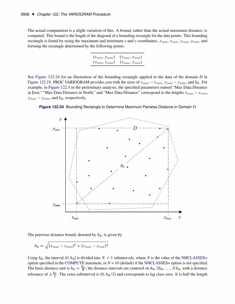
9906 F Chapter 122: The VARIOGRAM Procedure
The actual computation is a slight variation of this. A bound, rather than the actual maximum distance, iscomputed. This bound is the length of the diagonal of a bounding rectangle for the data points. This boundingrectangle is found by using the maximum and minimum x and y coordinates, xmax ; xmin ; ymax ; ymin , andforming the rectangle determined by the following points:
.xmin ; ymax / .xmax ; ymax /
.xmin ; ymin/ .xmax ; ymin/
See Figure 122.24 for an illustration of the bounding rectangle applied to the data of the domain D inFigure 122.19. PROC VARIOGRAM provides you with the sizes of xmax � xmin , ymax � ymin , and hb . Forexample, in Figure 122.4 in the preliminary analysis, the specified parameters named “Max Data Distancein East,” “Max Data Distance in North,” and “Max Data Distance” correspond to the lengths xmax � xmin ,ymax � ymin , and hb , respectively.
Figure 122.24 Bounding Rectangle to Determine Maximum Pairwise Distance in Domain D
The pairwise distance bound, denoted by hb , is given by
hb D
q.xmax � xmin/2 C .ymax � ymin/2
Using hb , the interval .0; hb� is divided into N C 1 subintervals, where N is the value of the NHCLASSES=option specified in the COMPUTE statement, or N = 10 (default) if the NHCLASSES= option is not specified.The basic distance unit is h0 D hb
N; the distance intervals are centered on h0; 2h0; : : : ; Nh0, with a distance
tolerance of ˙h0
2. The extra subinterval is .0; h0=2/ and corresponds to lag class zero. It is half the length
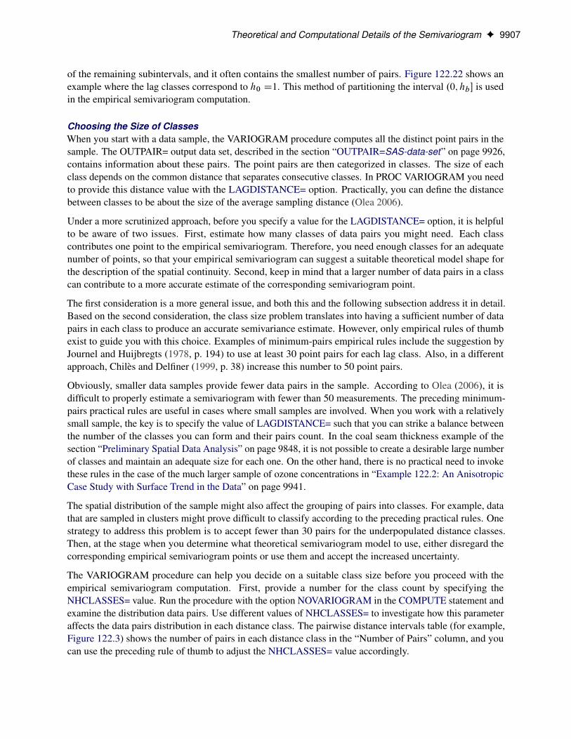
Theoretical and Computational Details of the Semivariogram F 9907
of the remaining subintervals, and it often contains the smallest number of pairs. Figure 122.22 shows anexample where the lag classes correspond to h0 D1. This method of partitioning the interval .0; hb� is usedin the empirical semivariogram computation.
Choosing the Size of ClassesWhen you start with a data sample, the VARIOGRAM procedure computes all the distinct point pairs in thesample. The OUTPAIR= output data set, described in the section “OUTPAIR=SAS-data-set” on page 9926,contains information about these pairs. The point pairs are then categorized in classes. The size of eachclass depends on the common distance that separates consecutive classes. In PROC VARIOGRAM you needto provide this distance value with the LAGDISTANCE= option. Practically, you can define the distancebetween classes to be about the size of the average sampling distance (Olea 2006).
Under a more scrutinized approach, before you specify a value for the LAGDISTANCE= option, it is helpfulto be aware of two issues. First, estimate how many classes of data pairs you might need. Each classcontributes one point to the empirical semivariogram. Therefore, you need enough classes for an adequatenumber of points, so that your empirical semivariogram can suggest a suitable theoretical model shape forthe description of the spatial continuity. Second, keep in mind that a larger number of data pairs in a classcan contribute to a more accurate estimate of the corresponding semivariogram point.
The first consideration is a more general issue, and both this and the following subsection address it in detail.Based on the second consideration, the class size problem translates into having a sufficient number of datapairs in each class to produce an accurate semivariance estimate. However, only empirical rules of thumbexist to guide you with this choice. Examples of minimum-pairs empirical rules include the suggestion byJournel and Huijbregts (1978, p. 194) to use at least 30 point pairs for each lag class. Also, in a differentapproach, Chilès and Delfiner (1999, p. 38) increase this number to 50 point pairs.
Obviously, smaller data samples provide fewer data pairs in the sample. According to Olea (2006), it isdifficult to properly estimate a semivariogram with fewer than 50 measurements. The preceding minimum-pairs practical rules are useful in cases where small samples are involved. When you work with a relativelysmall sample, the key is to specify the value of LAGDISTANCE= such that you can strike a balance betweenthe number of the classes you can form and their pairs count. In the coal seam thickness example of thesection “Preliminary Spatial Data Analysis” on page 9848, it is not possible to create a desirable large numberof classes and maintain an adequate size for each one. On the other hand, there is no practical need to invokethese rules in the case of the much larger sample of ozone concentrations in “Example 122.2: An AnisotropicCase Study with Surface Trend in the Data” on page 9941.
The spatial distribution of the sample might also affect the grouping of pairs into classes. For example, datathat are sampled in clusters might prove difficult to classify according to the preceding practical rules. Onestrategy to address this problem is to accept fewer than 30 pairs for the underpopulated distance classes.Then, at the stage when you determine what theoretical semivariogram model to use, either disregard thecorresponding empirical semivariogram points or use them and accept the increased uncertainty.
The VARIOGRAM procedure can help you decide on a suitable class size before you proceed with theempirical semivariogram computation. First, provide a number for the class count by specifying theNHCLASSES= value. Run the procedure with the option NOVARIOGRAM in the COMPUTE statement andexamine the distribution data pairs. Use different values of NHCLASSES= to investigate how this parameteraffects the data pairs distribution in each distance class. The pairwise distance intervals table (for example,Figure 122.3) shows the number of pairs in each distance class in the “Number of Pairs” column, and youcan use the preceding rule of thumb to adjust the NHCLASSES= value accordingly.

9908 F Chapter 122: The VARIOGRAM Procedure
PROC VARIOGRAM displays a rounded value of the distance between the lag bounds as the “Lag Distance”parameter in the pairs information table (see Figure 122.5) or the pairwise distances histogram (see Fig-ure 122.4), which you can use for the LAGDISTANCE= specification. However, this is only one tool. For thesemivariogram computation you can specify your own LAGDISTANCE= value based on your experience.Smaller LAGDISTANCE= values result in fewer data pairs in the classes. In that sense, you might findsmaller values useful when you work with large samples so that you obtain more semivariogram points. Also,if the LAGDISTANCE= value is too large, you might end up “wasting” too many point pairs in fewer classesat the expense of computing fewer semivariogram points and no significant accuracy gains in the estimation.
As explained earlier, depending on the sample size and its spatial distribution you might have classes withfewer points than what the practical rules advise. Most commonly, the deficient distance classes are thelimiting ones close to the origin h D 0 and the most remote ones at large h. The classes near the origincorrespond to lags 0 and 1. These lags are crucial because the empirical semivariogram in small distances hcharacterizes the process smoothness and can help you detect the presence of a nugget effect. However, asdiscussed in the section “Distance Classification” on page 9903, lag zero is half the size of the rest of theclasses by definition, so it can be expected to violate the rule of thumb for the number of pairs in a class.
The classes located at higher and extreme distances within a spatial domain are often not accounted for in theempirical semivariogram. The fewer pairs that can be formed in these distances do not allow for an accurateassessment of the spatial correlation, as is explained in the following section.
Spatial Extent of the Empirical SemivariogramGiven your choice for the LAGDISTANCE= value in your spatial domain, the following paragraphs provideguidelines on how many classes to consider when you compute the empirical semivariogram.
Obviously, you want to include no more classes beyond the limit where the pairs count falls below theminimum-pairs empirical rule threshold, as discussed in the preceding subsection. PROC VARIOGRAMprovides you with a visual way to inspect this upper limit, if you decide to make use of the minimum-pairsempirical rule. In particular, specify your threshold choice for the minimum pairs per class by using theTHRESHOLD= parameter for the PLOTS=PAIRS option.
Then, the procedure produces in the pairwise distances histogram a reference line at the specified THRESH-OLD= value, which leaves below the line all lags whose pairs count is lower than the threshold value; see,for example, Figure 122.4. The last lag class whose pair population is above the THRESHOLD= value isreported in the pairs information table as “Highest Lag With Pairs > Threshold.” This value is not a recom-mendation for the MAXLAGS= option, but rather is an upper limit for your choice. Detailed informationabout the pairs count in each class is displayed in the corresponding pairwise distance intervals table, asFigure 122.3 demonstrates.
The preceding suggests that you have an upper limit indication, but you still need some criterion to decidehow many lags to include in the semivariogram estimation. The criterion is the extent of spatial dependencein your domain.
Spatial dependence can exist beyond your domain limits. However, you have no data past your domain scaleto define a range for larger-scale spatial dependencies. As you look for pairs of data that are gradually fartherapart, the number of pairs naturally decreases with distance. The pairs at the more distant classes might be sofew that they are likely to be independent with respect to the spatial dependence scale that you can detect. Ifyou include the largest distances in your empirical semivariogram plot, then these pairs only contribute addednoise. In the same sense, you cannot explore in detail spatial dependencies in scales smaller than an averageminimum distance between your data. The nugget effect represents then microscale correlations whose effectis evident in your working scale.

Theoretical and Computational Details of the Semivariogram F 9909
You specify the spatial dependence extent with commonly used measures such as the correlation range (orcorrelation length) � and the correlation radius hc . Both are defined in a similar manner. The correlationrange � is the distance at which the covariance is 5% of its value at h D 0, and shows that beyond � thecovariance is considered to be negligible. The correlation radius hc is the distance at which the covarianceis about half the variance at h D 0, and indicates the distance over which significant correlations prevail(Christakos 1992, p. 76). The physical meanings of these measures are similar to that of the semivariogramrange. Also, the effective range r� used in asymptotically increasing semivariance models has essentiallythe same definition as the correlation range � (see the section “Theoretical Semivariogram Models” onpage 9892).
A rough estimate of the correlation extent measures might be available from previous studies of a similar site,or from prior information about related measurements. In such an event, you typically want to consider amaximum pairwise distance that does not exceed the length of two or three correlation radii, or one and ahalf correlation ranges. You can then specify the MAXLAGS= value on the basis of the lags that fit in thatdistance.
When you have no estimates of correlation extent measures, you can use first use a crude measure to getstarted with your analysis: you can typically expect MAXLAGS= to be about half of the lag classes shown inthe pairwise distances histogram.
Then, if necessary, you can refine your MAXLAGS= choice by using the following maximum lags rule ofthumb: Journel and Huijbregts (1978, p. 194) advise considering lags up to about half of the extreme distancebetween data in the direction of interest. The VARIOGRAM procedure assists you in this task by providingthe overall extreme data distance hb , in addition to the extreme data distances in the vertical and horizontalaxes directions. For example, hb is reported in the pairs information table as “Maximum Data Distance” (seeFigure 122.5), and in the pairwise distances histogram as “Max Data Distance” (see Figure 122.4).
Overall, avoid significant deviations from the maximum lags rule of thumb. As was stated earlier, aMAXLAGS= value that takes you well beyond the half-extreme distance between data in a given directionmight give you limited accuracy in the empirical semivariance estimates at higher distances. At the otherend, a value of MAXLAGS= that is too small might lead you to omit important information about the spatialstructure that potentially lies within the range of distances you skipped.
Semivariance Computation
With the classification of a point pair PiPj into an angle/distance class, as shown earlier in this section, thesemivariance computation proceeds as follows.
Denote all pairs that PiPj belong to angle class Œ�k � ı�k; �k C ı�k/ and distance class L D L.PiPj / asN.�k; L/. For example, based on Figure 122.20 and Figure 122.21, P1P2 belongs to N.60ı; 1/.
Let j N.�k; L/ j denote the number of such pairs. The component of the standard (or method of moments)semivariance that correspond to angle/distance class N.�k; L/ is given by
O .hk/ D1
2 j N.�k; L/ j
XPiPj2N.�k ;L/
ŒV .si / � V.sj /�2
where hk is the average distance in class N.�k; L/; that is,
hk D1
j N.�k; L/ j
XPiPj2N.�k ;L/
j PiPj j

9910 F Chapter 122: The VARIOGRAM Procedure
The robust version of the semivariance is given by
N .hk/ D‰4.hk/
2Œ0:457C 0:494=N.�k; L/�
where
‰.hk/ D1
N.�k; L/
XPiPj2N.�k ;L/
ŒV .si / � V.sj /�12
This robust version of the semivariance is computed when you specify the ROBUST option in the COMPUTEstatement in PROC VARIOGRAM.
PROC VARIOGRAM computes and writes to the OUTVAR= data set the quantities hk; �k; L;N.�k; L/; O .h/,and N .h/.
Empirical Semivariograms and Surface Trends
It was stressed in the beginning of the section “Theoretical and Computational Details of the Semivariogram”on page 9897 that if your data are not free of nonrandom surface trends, then the empirical semivarianceO z.h/ you obtain from PROC VARIOGRAM represents a pseudo-semivariance rather than an estimate of thetheoretical semivariance z.h/.
In practice, two major difficulties appear. First, you might have no knowledge of underlying surface trendsin your SRF Z.s/. It can be possible to have this information when you deal with a repetitive phenomenon(Chilès and Delfiner 1999, p. 123), or if you work within a subdomain of a broader region with knowncharacteristics; often, though, this is not the case. Second, even if you suspect the existence of an underlyingnonrandom trend, its precise nature might be unknown (Cressie 1993, p. 114, 162).
Based on the last remark, the criteria to define the exact form of a surface trend can be subjective. However,statistical methods can identify the presence and remove an estimate of such a trend. Different trend formscan be estimated in your SRF depending on the trend estimation model that you choose. This choice canlead to different degrees of smoothing in the residual random fluctuations. It might also have an effect onthe residuals spatial structure characterization, because trend removals with different models are essentiallydifferent operations acting upon the values of your original observations. Following the comment by Chilèsand Delfiner (1999, section 2.7.3), there are as many semivariograms of residuals as there are ways ofestimating the trend. The same source also examines the introduction of bias in the semivariance of theresiduals as a side effect of trend removal processes. This bias is small when you examine distances close tothe origin h D 0, and it can increase with distance.
Keeping in mind the preceding remarks, an approach you can take is to use one of the many predictivemodeling tools in SAS/STAT software to estimate the unknown trend. Then you use PROC VARIOGRAM toanalyze the residuals after you remove the trend. If the resulting model does not require too many degrees offreedom (such as if you use a low-order polynomial), then this approach might be sufficient. The section“Analysis with Surface Trend Removal” on page 9945 demonstrates how to use PROC GLM (see Chapter 46,“The GLM Procedure”) for that purpose.
Apart from the standard semivariogram analysis, you can attempt to fit a theoretical semivariogram model toyour empirical semivariogram if (a) either the analysis itself or your knowledge of the SRF does not clearlysuggest the presence of any surface trend, or (b) the analysis can indicate a potentially trend-free direction,along which your data have a constant mean.

Theoretical Semivariogram Model Fitting F 9911
For example, you might observe overall similar values in your data. This can be an indication that your dataare free of nonrandom trends, or that a very mild trend is present. The case falls under the preceding option(a). A very mild trend still allows a good determination of the semivariance at short distances according toChilès and Delfiner (1999, p. 125), and this can be sufficient for your spatial prediction goal. An analysis ofthis type is assumed in the section “Preliminary Spatial Data Analysis” on page 9848.
If you observe similar values locally across a particular direction, this an instance of option (b). Olea (2006)suggests recognizing a trend-free direction as being perpendicular to the axis of the maximum dip in the valuesof Z.s/. If you suspect that at least one such direction exists for your data, then run PROC VARIOGRAMfor a series of directions in the angular vicinity. The trend-free direction, if it exists, coincides with the onewhose pseudo-semivariogram exhibits minimal increase with distance; see “Example 122.3: Analysis withoutSurface Trend Removal” on page 9955 for a demonstration of this approach. However, you cannot testZ.s/ for anisotropy in this case, because you can investigate the semivariogram only in the single trend-freedirection (Olea 1999, p. 76). Chilès and Delfiner (1999, section 2.7.4) suggest fitting a theoretical model in atrend-free direction only if the hypothesis of an isotropic semivariogram appears reasonable in your analysis.
As a result, you need to be very cautious when you choose to perform semivariogram analysis on data youhave not previously examined for surface trends. In this event, both of the options (a) and (b) that werereviewed in the preceding paragraphs rely mostly on empirical and subjective criteria. As noted in thissection, a degree of subjectivity exists in the selection of the surface trend itself. This fact suggests that asignificant part of the semivariogram analysis is based on metastatistical decisions and on your understandingof your data and the physical considerations that govern your study. In any case, as shown in the section“Theoretical and Computational Details of the Semivariogram” on page 9897, your semivariogram analysisrelies fundamentally on the use of trend-free data.
Theoretical Semivariogram Model FittingYou can choose between two approaches to select a theoretical semivariogram model and fit the empiricalsemivariance. The first one is manual fitting, in which a theoretical semivariogram model is selected basedon visual inspection of the empirical semivariogram. For example, see Hohn (1988, p. 25) and commentsfrom defendants of this approach in Olea (1999, p. 82). The second approach is to perform model fitting inan automated manner. For this task you can use methods such as least squares, maximum likelihood, androbust methods (Cressie 1993, section 2.6).
The VARIOGRAM procedure features automated semivariogram model fitting that uses the weighted leastsquares (WLS) or the ordinary least squares (OLS) method. Use the MODEL statement to request that specificmodel forms or an array of candidate models be tested for optimal fitting to the empirical semivariance.
Assume that you compute first the empirical semivariance �z .h/ at MAXLAGS=k distance classes, where �z .h/ can be either the classical estimate O z.h/ or the robust estimate N z.h/, as shown in the section“Theoretical and Computational Details of the Semivariogram” on page 9897. In fitting based on least squares,you want to estimate the parameters vector � of the theoretical semivariance z.h/ that minimizes the sumof square differences R.�/ given by the expression
R.�/ D
kXiD1
wi2� �z .hi / � z.hi I�/
�2
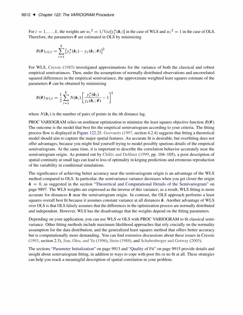
9912 F Chapter 122: The VARIOGRAM Procedure
For i D 1; : : : ; k, the weights are wi 2 D 1=VarŒ �z .hi /� in the case of WLS and wi 2 D 1 in the case of OLS.Therefore, the parameters � are estimated in OLS by minimizing
R.�/OLS D
kXiD1
� �z .hi / � z.hi I�/
�2For WLS, Cressie (1985) investigated approximations for the variance of both the classical and robustempirical semivariances. Then, under the assumptions of normally distributed observations and uncorrelatedsquared differences in the empirical semivariance, the approximate weighted least squares estimate of theparameters � can be obtained by minimizing
R.�/WLS D1
2
kXiD1
N.hi /
� �z .hi /
z.hi I�/� 1
�2
where N.hi / is the number of pairs of points in the ith distance lag.
PROC VARIOGRAM relies on nonlinear optimization to minimize the least squares objective function R.�/.The outcome is the model that best fits the empirical semivariogram according to your criteria. The fittingprocess flow is displayed in Figure 122.25. Goovaerts (1997, section 4.2.4) suggests that fitting a theoreticalmodel should aim to capture the major spatial features. An accurate fit is desirable, but overfitting does notoffer advantages, because you might find yourself trying to model possibly spurious details of the empiricalsemivariogram. At the same time, it is important to describe the correlation behavior accurately near thesemivariogram origin. As pointed out by Chilès and Delfiner (1999, pp. 104–105), a poor description ofspatial continuity at small lags can lead to loss of optimality in kriging predictions and erroneous reproductionof the variability in conditional simulations.
The significance of achieving better accuracy near the semivariogram origin is an advantage of the WLSmethod compared to OLS. In particular, the semivariance variance decreases when you get closer the originh D 0, as suggested in the section “Theoretical and Computational Details of the Semivariogram” onpage 9897. The WLS weights are expressed as the inverse of this variance; as a result, WLS fitting is moreaccurate for distances h near the semivariogram origin. In contrast, the OLS approach performs a leastsquares overall best fit because it assumes constant variance at all distances h. Another advantage of WLSover OLS is that OLS falsely assumes that the differences in the optimization process are normally distributedand independent. However, WLS has the disadvantage that the weights depend on the fitting parameters.
Depending on your application, you can use WLS or OLS with PROC VARIOGRAM to fit classical semi-variance. Other fitting methods include maximum likelihood approaches that rely crucially on the normalityassumption for the data distribution, and the generalized least squares method that offers better accuracybut is computationally more demanding. You can find extensive discussions about these issues in Cressie(1993, section 2.3), Jian, Olea, and Yu (1996), Stein (1988), and Schabenberger and Gotway (2005).
The sections “Parameter Initialization” on page 9913 and “Quality of Fit” on page 9915 provide details andinsight about semivariogram fitting, in addition to ways to cope with poor fits or no fit at all. These strategiescan help you reach a meaningful description of spatial correlation in your problem.

Theoretical Semivariogram Model Fitting F 9913
Figure 122.25 Semivariogram Fitting Process Flowchart
Parameter Initialization
An important stage when you prepare for the model fitting process is initialization of the model parameters.As stated earlier, nonlinear optimization techniques are used in the fitting process. These techniques assist inthe estimation of the model parameters, and being nonlinear means they can be very sensitive to selection ofthe initial values.
You can specify initial values close to the expected estimates when you have a relatively simple problem,such as in the example of the section “Getting Started: VARIOGRAM Procedure” on page 9847. In the caseof nested models the selection of initial values can be more challenging because you have to assess the levelof contribution for each one of the nested components.

9914 F Chapter 122: The VARIOGRAM Procedure
The VARIOGRAM procedure features automatic selection of initial values based on the recommendations inJian, Olea, and Yu (1996). Specifically, if you compute the estimated empirical semivariogram O z.h/ at klags, then:
� The default initial nugget effect cn;0 is
cn;0 D Max�0; O z.h1/ �
h1
h2 � h1Œ O z.h2/ � O z.h1/�
�� The default initial slope �0;02 and initial exponent a0;0 for the power model are
�0;02DŒ O z.hk�2/C O z.hk�1/C O z.hk/� =3 � cn;0
hk � h1
a0;0 D 1
� The default initial scale �0;02 and initial range a0;0 for all other models are
�0;02DŒ O z.hk�2/C O z.hk�1/C O z.hk/�
3� cn;0
a0;0 D 0:5hk
When you use the Matérn form, PROC VARIOGRAM sets the default initial value for the Matérn smoothnessto �0 D 1.
These rules are observed in the case of single, non-nested model fitting, and they are slightly modifiedto apply for nested model fitting as follows: Assume that you want to fit a nested model composed of mstructures. As stated in the section “Nested Models” on page 9897, the nugget effect is a single parameter andis independent of the number of nested structures in a model. Also, the sum of the nested structure scales andthe nugget effect, if any, must be equal to the total variance. For this reason, PROC VARIOGRAM simplydivides the initial scale value it would assign to a non-nested model into m components �0;0;12; : : : ; �0;0;m2.For the range parameter, the VARIOGRAM procedure sets the initial range a0;0;1 of the first nested structureequal to the value it would assign to a non-nested model initial range. Then, the initial range a0;0;m of them-component is set recursively to half the value of the initial range a0;0;m�1 of the .m � 1/-component.
Your empirical semivariogram must have nonmissing estimates at least at three lags so that you can use theautomated fitting feature in PROC VARIOGRAM. Overall, if you specify a model form with q parameters tofit to an empirical semivariogram with nonmissing estimates at k lags, then the fitting problem is well-definedonly when the degrees of freedom are DF D k � q � 0.
A potential numerical issue is that fitting could momentarily lead the fitting parameters to near-zero semivari-ance values at lags away from zero distance. The theoretical semivariance is always positive for any distancelarger than zero, and this is also a requirement for the numerical computation of R.�/WLS in weighted leastsquares fitting. Such numerical issues are unlikely but possible, depending on the data set you use and theparameter initial values. If an event of nonpositive semivariance at a given lag occurs during an iteration,then PROC VARIOGRAM transparently adds a minimal amount of variance at that lag for the specificiteration. You can control this amount of variance with the NEPSILON= option of the MODEL statement. Itis recommended that you leave this parameter at its default value.
The section concludes with a reminder of the fitting process sensitivity to the initial parameter valuesselection. The VARIOGRAM procedure facilitates this selection for you by using the simple rules shown

Theoretical Semivariogram Model Fitting F 9915
earlier. However, the suggested initial values might not always be the best choice. In simple cases, suchas the introductory example in the section “Getting Started: VARIOGRAM Procedure” on page 9847, thisapproach is very convenient and effective.
In principle, you are strongly encouraged to experiment with initial values. You want to make sure that thefitting process leads the model parameters to converge to estimates that make sense for your problem. Whena parameter estimate seems unreasonable on the basis of your problem specification (for example, a modelscale might be estimated to be 10 times the size of your sample variance, or the estimate of a range might bezero), PROC VARIOGRAM produces a note to let you know about a potentially ambiguous fit. These issuesare examined in more detail in the section “Quality of Fit” on page 9915.
Parameter Estimates
When the fit process is complete, the VARIOGRAM procedure produces the “Parameter Estimates” tablewith information about the fitted model parameters. The table includes estimates of the parameters, theirapproximate standard error, the statistical degrees of freedom DF, the corresponding t statistic, and itsapproximate p-value. For a model with q parameters that fits an empirical semivariogram of k nonmissinglags, DF D k � q.
NOTE: Parameter estimates might have nonzero standard errors even in the rather extreme case whereDF D 0. This can typically occur when there are active optimization constraints in the fitting process.
You can request the confidence intervals for the parameter estimates of a fitted model by specifying the CLoption of the MODEL statement. These confidence intervals are computed using the Wald-based formula
b̌i ˙ stderri � t .k � q; 1 � ˛=2/
where b̌i is the ith parameter estimate, stderri is its estimated approximate standard error, t .k � q; 1� ˛=2/is the t statistic with DF D k � q degrees of freedom. The confidence intervals are only asymptotically valid.The significance level ˛ used in the construction of these confidence limits can be set with the ALPHA=option of the MODEL statement; the default value is ˛ D 0:05.
Specify the COVB and the CORRB options in the MODEL statement to request the approximate covarianceand approximate correlation matrices of the fitted parameters, respectively. These matrices are based on theoptimization process results. In agreement with reporting similar optimization output in SAS/STAT software,parameters with active restraints have zeros in the corresponding rows and columns in the covariance andcorrelation matrices, and display 1 in the correlation matrix diagonal.
Quality of Fit
The VARIOGRAM procedure produces a fit summary table to report about the goodness of fit. When youspecify multiple models to fit with the FORM=AUTO option in the MODEL statement, the VARIOGRAMprocedure uses two processes to rank the fitted models: The first one depends on your choice among availablefitting criteria. The second one is based on an operational classification of equivalent models in classes. Thetwo processes are described in more detail in the following subsections.
Overall, no absolutely correct way exists to rank and classify multiple models. Your choice of ranking criteriacould depend on your study specifications, physical considerations, or even your personal assessment offitting performance. The VARIOGRAM procedure provides you with fitting and comparison features tofacilitate and help you better understand the fitting process.

9916 F Chapter 122: The VARIOGRAM Procedure
Fitting CriteriaThe fit summary table ranks multiple models on the basis of one or more fitting criteria that you can specifywith the CHOOSE= option of the MODEL statement, as explained in the section “Syntax: VARIOGRAMProcedure” on page 9861. Currently, the VARIOGRAM procedure offers two numerical criteria (for which asmaller value indicates a better fit) and a qualitative criterion:
� The residual sum of squares error (SSE) is based on the objective function of the fitting process. Whenthe specified method is weighted least squares, the sum of squares of the weighted differences (WSSE)is computed according to the expression
WSSE DkXiD1
wi2� �z .hi / � z.hi I�/
�2where �z .hi / can be either the classical or robust semivariance estimate of the theoretical semivariance z.hi I�/ at the ith lag and the weights wi 2 are taken at lags i D 1; : : : ; k. When you specify theMETHOD=OLS option in the MODEL, the weights wi 2 D 1 for i D 1; : : : ; k, and the SSE isexpressed as
SSE DkXiD1
� �z .hi / � z.hi I�/
�2� Akaike’s information criterion (AIC) is included in the fit summary table when there is at least one
nonfixed parameter. In its strict definition, AIC assumes that the model errors are normally andindependently distributed. This assumption is not correct in the semivariance fitting analysis. However,the AIC can be also defined in an operational manner on the basis of the weighted squared error sumWSSE as
AIC D kln�
WSSEk
�C 2q
for k lags and q model parameters; see, for example, Olea (1999, p. 84). The operational definition of theAIC is provided as an additional criterion for the comparison of fitted models in PROC VARIOGRAM.
The AIC expression suggests that when you specify multiple models with the FORM=AUTO option inthe MODEL statement, all models with the same number of parameters are ranked in the same way bythe AIC and the WSSE criteria. Among models with the same WSSE value, AIC ranks higher the oneswith fewer parameters.
� The third qualitative criterion enables you to classify multiple models based on their convergencestatus. A model is sent to the bottom of the ranking table if the parameter estimation optimization failsto converge or fitting is unsuccessful due to any other issue. These two cases are distinguished by thedifferent notes they produce in the fit summary ODS table. If you specify the STORE statement to savethe fitting output in an item store, then models that have failed to fit are not passed to the item store.
With respect to convergence status, PROC VARIOGRAM ranks higher those models that have successfullycompleted the fitting process. It might occur that the selection of parameter initial values, physical considera-tions about the forms that are used for the fit, or numerical aspects of the nonlinear optimization could resultin ambiguous fits. For example, you might see that model parameters converge at or near their boundary
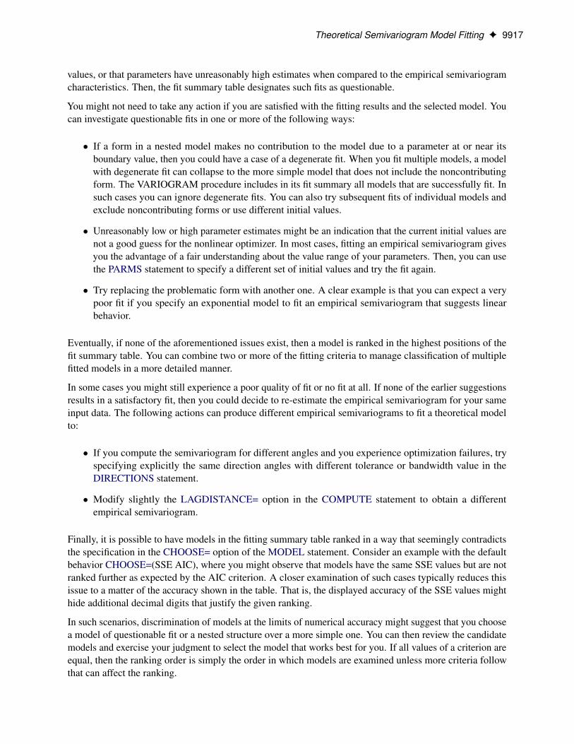
Theoretical Semivariogram Model Fitting F 9917
values, or that parameters have unreasonably high estimates when compared to the empirical semivariogramcharacteristics. Then, the fit summary table designates such fits as questionable.
You might not need to take any action if you are satisfied with the fitting results and the selected model. Youcan investigate questionable fits in one or more of the following ways:
� If a form in a nested model makes no contribution to the model due to a parameter at or near itsboundary value, then you could have a case of a degenerate fit. When you fit multiple models, a modelwith degenerate fit can collapse to the more simple model that does not include the noncontributingform. The VARIOGRAM procedure includes in its fit summary all models that are successfully fit. Insuch cases you can ignore degenerate fits. You can also try subsequent fits of individual models andexclude noncontributing forms or use different initial values.
� Unreasonably low or high parameter estimates might be an indication that the current initial values arenot a good guess for the nonlinear optimizer. In most cases, fitting an empirical semivariogram givesyou the advantage of a fair understanding about the value range of your parameters. Then, you can usethe PARMS statement to specify a different set of initial values and try the fit again.
� Try replacing the problematic form with another one. A clear example is that you can expect a verypoor fit if you specify an exponential model to fit an empirical semivariogram that suggests linearbehavior.
Eventually, if none of the aforementioned issues exist, then a model is ranked in the highest positions of thefit summary table. You can combine two or more of the fitting criteria to manage classification of multiplefitted models in a more detailed manner.
In some cases you might still experience a poor quality of fit or no fit at all. If none of the earlier suggestionsresults in a satisfactory fit, then you could decide to re-estimate the empirical semivariogram for your sameinput data. The following actions can produce different empirical semivariograms to fit a theoretical modelto:
� If you compute the semivariogram for different angles and you experience optimization failures, tryspecifying explicitly the same direction angles with different tolerance or bandwidth value in theDIRECTIONS statement.
� Modify slightly the LAGDISTANCE= option in the COMPUTE statement to obtain a differentempirical semivariogram.
Finally, it is possible to have models in the fitting summary table ranked in a way that seemingly contradictsthe specification in the CHOOSE= option of the MODEL statement. Consider an example with the defaultbehavior CHOOSE=(SSE AIC), where you might observe that models have the same SSE values but are notranked further as expected by the AIC criterion. A closer examination of such cases typically reduces thisissue to a matter of the accuracy shown in the table. That is, the displayed accuracy of the SSE values mighthide additional decimal digits that justify the given ranking.
In such scenarios, discrimination of models at the limits of numerical accuracy might suggest that you choosea model of questionable fit or a nested structure over a more simple one. You can then review the candidatemodels and exercise your judgment to select the model that works best for you. If all values of a criterion areequal, then the ranking order is simply the order in which models are examined unless more criteria followthat can affect the ranking.

9918 F Chapter 122: The VARIOGRAM Procedure
Classes of EquivalenceThe fit summary that is produced after fitting multiple models further categorizes the ranked models inclasses of equivalence. Equivalence classification is an additional investigation that is unrelated to the rankingcriteria presented in the previous subsection; it is an operational criterion that provides you with a qualitativeoverview of multiple model fit performance under given fitting conditions.
To examine model equivalence, the VARIOGRAM procedure computes the semivariances for each one ofthe fitted models at a set of distances. For any pair of consecutively ranked models, if the sum of theirsemivariance absolute differences at all designated distances is smaller than the tolerance specified by theEQUIVTOL= parameter, then the two models are deemed equivalent and placed in the same class; otherwise,they are placed in different classes. Equivalence classification depends on the existing ranking; hence theresulting classes can differ when you specify different ranking criteria in the CHOOSE= option of theMODEL statement.
The equivalence class numbers start at 1 for the top-ranked model in the fit summary table. You can considerthe top model of each equivalence class to be a representative of the class behavior. When you specify that fitplots be produced and there are equivalence classes, the plot displays the equivalence classes and the legenddesignates each one by its representative model.
Consequently, if an equivalence class contains multiple members after a fit, then all of its members producein general the exact same semivariogram. A typical reason could be that the fitting process estimates of scaleparameters are at or close to their zero boundaries in one or more nested forms in a model. In such cases, thebehavior of this model reduces to the behavior of its nested components with nonzero parameters. Whenone or more models share this situation or have the same contributing nested forms, they could end up asmembers of the same equivalence class depending on the ranking criteria.
It is not necessary for all models in the same equivalence class to produce the exact same semivariogram. If afit of two obviously different forms involves semivariance values that are small enough for the equivalencecriterion to be satisfied by the default value of the EQUIVTOL= option, then you might need to specify aneven smaller value in the EQUIVTOL= option to rank these two models in separate equivalence classes.
Fitting with Matérn Forms
When you use a Matérn form in the fitting process, it is possible that the fitting optimizer might encounternumerical difficulties if it tries to push the smoothing parameter � towards increasingly high values. TheVARIOGRAM procedure addresses this issue by imposing an amply elevated upper bound of 1,000,000 onthe smoothness values it processes. The section “Characteristics of Semivariogram Models” on page 9893mentions that � ! 1 gives the Gaussian model. In the scenario of progressively increasing smoothnessvalues, PROC VARIOGRAM acknowledges that the Matérn form behavior tends asymptotically to becomeGaussian and replaces automatically the Matérn with a Gaussian form in the model. Subsequently, fittingresumes with the resulting model.
If you explore fitting of multiple models, then any duplicate models that might occur due to Matérn-to-Gaussian form conversions are fitted only once. Also, if a nested model has more than one Matérn form, thenthe fitting process checks one of them at a time about whether they need to be replaced by a Gaussian form.Consequently, following the switch of one Matérn form, the fitting process starts anew with the resultingmodel before any decisions for additional form conversions are made.
Replacement of the Matérn form with the Gaussian form occurs by default when � > 10; 000. However, youcan control this threshold value with the MTOGTOL= parameter of the MODEL statement. Practically, theMatérn form starts to resemble the Gaussian behavior for � values that are about � > 10. If you encounter

Autocorrelation Statistics F 9919
such conversions of the Matérn form into Gaussian and you prefer to set a lower � threshold for the conversionthan the default, you might experience improved code performance because computation of the Matérnsemivariance can be numerically demanding.
Autocorrelation StatisticsSpatial autocorrelation measures offer you additional insight into the interdependence of spatial data. Thesemeasures quantify the correlation of an SRFZ.s/ with itself at different locations, and they can be very usefulwhether you have information at exact locations (point-referenced data) or measurements that characterize anarea type such as counties, census tracts, zip codes, and so on (areal data).
As in the semivariogram computation, a key issue for the autocorrelation statistics is that you work with a setzi of measurements, i D 1; : : : ; n, that are free of nonrandom surface trends and have a constant mean.
Autocorrelation Weights
In general, the choice of a weighting scheme is subjective. You can obtain different results by using differentschemes, options, and parameters. PROC VARIOGRAM offers you considerable flexibility in choosingweights that are appropriate for prior considerations such as different hypotheses about neighboring areas,definition of the neighborhood structure, and accounting for natural barriers or other spatial characteristics;see the discussion in Cliff and Ord (1981, p. 17). As stressed for all types of spatial analysis, it is importantto have good knowledge of your data. In the autocorrelation statistics, this knowledge can help you avoidspurious correlations when you choose the weights.
The starting point is to assign individual weights to each one of the n data values zi , i D 1; : : : ; n, withrespect to the rest. An n � n matrix of weights is thus defined, such that for any two locations si and sj , theweight wij denotes the effect of the value zi at location si on the value zj at location sj . Depending on thenature of your study, the weights wij need not be symmetric; that is, it can be true that wij ¤ wj i .
Binary and Nonbinary WeightsThe weights wij can be either binary or nonbinary values. Binary values of 1 or 0 are assigned if the SRFZ.si / at one location si is deemed to be connected or not, respectively, to its value Z.sj / at another locationsj . Nonbinary values can be used in the presence of more refined measures of connectivity between anytwo data points Pi and Pj . PROC VARIOGRAM offers a choice between a binary and a distance-basednonbinary weighting scheme.
In the binary weighting scheme the weight wij D 1 if the data pair at si and sj is closer than the user-defined distance that is defined by the LAGDISTANCE= option, and wij D 0 if i D j or in any othercase. For that reason, in the COMPUTE statement, if you specify the WEIGHTS=BINARY suboption ofthe AUTOCORRELATION option when the NOVARIOGRAM option is also specified, then you must alsospecify the LAGDISTANCE= option.
The nonbinary weighting scheme is based on the pair distances and is invoked with theWEIGHTS=DISTANCE suboption of the AUTOCORRELATION option. PROC VARIOGRAM uses avariation of the Pareto form functional to set the weights. Namely, the autocorrelation weight for every pointpair Pi and Pj located at si and sj , respectively, is defined as
wij D s1
1C j h jp
where h D si � sj and p � 0 and s � 0 are user-defined parameters for the adjustment of the weights.

9920 F Chapter 122: The VARIOGRAM Procedure
In particular, the power parameter p is specified in the POWER= option of the DISTANCE suboption withinthe AUTOCORRELATION option. The default value for this parameter is p = 1. Also, the scaling parameters is specified by the SCALE= option in the DISTANCE suboption of the AUTOCORRELATION option.The default value for the scaling parameter is s = 1. You can use the p and s parameters to adjust theactual values of the weights according to your needs. Variations in the scaling parameter s do not affect thecomputed values of the Moran’s I and Geary’s c autocorrelation coefficients that are introduced in the section“Autocorrelation Statistics Types” on page 9920.
Nonbinary Weights with Normalized DistancesPROC VARIOGRAM offers additional flexibility in the DISTANCE weighting scheme through an optionto use normalized pair distances. You can invoke this feature by specifying the NORMALIZE option inthe DISTANCE suboption of the AUTOCORRELATION option. In this case, the distances used in thedefinition of the weights are normalized by the maximum pairwise distance hb (see the section “Computationof the Distribution Distance Classes” on page 9905 and Figure 122.24); the weights are then defined aswij D s=Œ1C .j h j =hb/
p�.
Most likely, hb has a different value for different data sets. Hence, it is suggested that you avoid using theweights you obtain from the preceding equation and one data set for comparisons with the weights you derivefrom different data sets.
Symmetric and Asymmetric WeightsThe weighting schemes presented in the preceding paragraphs are symmetric; that is, wij D wj i for everydata pair at locations si and sj . However, you can also define asymmetric weights w0ij such thatX
j2J
w0ij D 1
for i D 1; 2; : : : ; n, where w0ij D wij =Pj2J wij , i D 1; 2; : : : ; n. In the distance-based scheme, J is the
set of all locations that form point pairs with the point at si . In the binary scheme, J is the set of the locationsthat are connected to si based on your selection of the LAGDISTANCE= option; see Cliff and Ord (1981,p. 18). The weights w0ij are row-averaged (or standardized by the count of their connected neighbors). Youcan apply row averaging in weights when you specify the ROWAVG option within either the BINARY orDISTANCE suboptions in the AUTOCORRELATION option.
Autocorrelation Statistics Types
One measure of spatial autocorrelation provided by PROC VARIOGRAM is Moran’s I statistic, which wasintroduced by Moran (1950) and is defined as
I Dn
.n � 1/S2W
Xi
Xj
wij vivj
where S2 D .n � 1/�1Pi v2i , and W D
Pi
Pj¤i wij .
Another measure of spatial autocorrelation in PROC VARIOGRAM is Geary’s c statistic (Geary 1954),defined as
c D1
2S2W
Xi
Xj
wij .zi � zj /2

Autocorrelation Statistics F 9921
These expressions indicate that Moran’s I coefficient makes use of the centered variable, whereas theGeary’s c expression uses the noncentered values in the summation.
Inference on these two statistic types comes from approximate tests based on the asymptotic distribution of Iand c, which both tend to a normal distribution as n increases. To this end, PROC VARIOGRAM calculatesthe means and variances of I and c. The outcome depends on the assumption made regarding the distributionZ.s/. In particular, you can choose to investigate any of the statistics under the normality (also known asGaussianity) or the randomization assumption. Cliff and Ord (1981) provided the equations for the meansand variances of the I and c distributions, as described in the following.
The normality assumption asserts that the random field Z.s/ follows a normal distribution of constant mean( NZ) and variance, from which the zi values are drawn. In this case, the I statistics yield
Eg ŒI � D �1
n � 1
and
Eg ŒI 2� D1
.nC 1/.n � 1/W 2.n2S1 � nS2 C 3W
2/
where S1 D 0:5Pi
Pj¤i .wij C wj i /
2 and S2 DPi .Pj wij C
Pj wj i /
2. The corresponding momentsfor the c statistics are
Eg Œc� D 1
and
VargŒc� D.2S1 C S2/.n � 1/ � 4W
2
2.nC 1/W 2
According to the randomization assumption, the I and c observations are considered in relation to all thedifferent values that I and c could take, respectively, if the n zi values were repeatedly randomly permutedaround the domain D. The moments for the I statistics are now
Er ŒI � D �1
n � 1
and
Er ŒI 2� DA1 C A2
.n � 1/.n � 2/.n � 3/W 2
where A1 D nŒ.n2 � 3n C 3/S1 � nS2 C 3W2�, A2 D �b2Œn.n � 1/S1 � 2nS2 C 6W 2�. The factor
b2 D m4=.m22/ is the coefficient of kurtosis that uses the sample moments mk D 1
n
Pi vki for k D 2; 4.
Finally, the c statistics under the randomization assumption are given by
Er Œc� D 1
and
VarrŒc� DB1 C B2 C B3
n.n � 2/.n � 3/W 2
9922 F Chapter 122: The VARIOGRAM Procedure
with B1 D .n � 1/S1Œn2 � 3nC 3 � .n � 1/b2�, B2 D �14.n � 1/S2Œn2 C 3n � 6 � .n2 � nC 2/b2�, and
B3 D W2Œn2 � 3 � b2.n � 1/
2�.
If you specify LAGDISTANCE= to be larger than the maximum data distance in your domain, the binaryweighting scheme used by the VARIOGRAM procedure leads to all weights wij D 1, i ¤ j . In this extremecase the preceding definitions can show that the variances of the I and c statistics become zero under eitherthe normality or the randomization assumption.
A similar effect might occur when you have collocated observations (see the section “Pair Formation” onpage 9900). The Moran’s I and Geary’s c statistics allow for the inclusion of such pairs in the computations.Hence, contrary to the semivariance analysis, PROC VARIOGRAM does not exclude pairs of collocated datafrom the autocorrelation statistics.
Interpretation
For Moran’s I coefficient, I > EŒI � indicates positive autocorrelation. Positive autocorrelation suggests thatneighboring values si and sj tend to have similar feature values zi and zj , respectively. When I < EŒI �,this is a sign of negative autocorrelation, or dissimilar values at neighboring locations. A measure of strengthof the autocorrelation is the size of the absolute difference j I � EŒI � j.
Geary’s c coefficient interpretation is analogous to that of Moran’s I. The only difference is that c > EŒc�indicates negative autocorrelation and dissimilarity, whereas c < EŒc� signifies positive autocorrelation andsimilarity of values.
The VARIOGRAM procedure uses the mathematical definitions in the preceding section to provide the ob-served and expected values, and the standard deviation of the autocorrelation coefficients in the autocorrelationstatistics table. The Z scores for each type of statistics are computed as
ZI DI � EŒI �p
VarŒI �
for Moran’s I coefficient, and
Zc Dc � EŒc�p
VarŒc�
for Geary’s c coefficient. PROC VARIOGRAM also reports the two-sided p-value for each coefficientunder the null hypothesis that the sample values are not autocorrelated. Smaller p-values correspond tostronger autocorrelation for both the I and c statistics. However, the p-value does not tell you whether theautocorrelation is positive or negative. Based on the preceding remarks, you have positive autocorrelationwhen ZI > 0 or Zc < 0, and you have negative autocorrelation when ZI < 0 or Zc > 0.
The Moran Scatter Plot
The Moran scatter plot (Anselin 1996) is a useful visual tool for exploratory analysis, because it enables youto assess how similar an observed value is to its neighboring observations. Its horizontal axis is based onthe values of the observations and is also known as the response axis. The vertical Y axis is based on theweighted average or spatial lag of the corresponding observation on the horizontal X axis. NOTE: The termspatial lag in the current context is unrelated to the concept of the semivariogram lag presented in the section“Distance Classification” on page 9903.

Computational Resources F 9923
The Moran scatter plot provides a visual representation of spatial associations in the neighborhood around eachobservation. You specify a neighborhood size with the LAGDISTANCE= option in the COMPUTE statement.The observations are represented by their standardized values; therefore only nonmissing observations areshown in the plot. For each one of those, the VARIOGRAM procedure computes the weighted average,which is the weighted mean value of its neighbors. Then, the centered weighted average is plotted against thestandardized observations. As a result, the scatter plot is centered on the coordinates (0; 0), and distances inthe plot are expressed in deviations from the origin (0; 0).
Depending on their position on the plot, the Moran plot data points express the level of spatial association ofeach observation with its neighboring ones. Conceptually, these characteristics differentiate the Moran plotfrom the semivariogram. The latter is typically used in geostatistics to depict spatial associations across thewhole domain as a continuous function of a distance metric.
You can find the data points on the Moran scatter plot in any of the four quadrants defined by the horizontalline y = 0 and the vertical line x = 0. Points in the upper right (or high-high) and lower left (or low-low)quadrants indicate positive spatial association of values that are higher and lower than the sample mean,respectively. The lower right (or high-low) and upper left (or low-high) quadrants include observations thatexhibit negative spatial association; that is, these observed values carry little similarity to their neighboringones.
When you use binary, row-averaged weights for the creation of the Moran scatter plot and in autocorrelationstatistics, Moran’s I coefficient is equivalent to the regression slope of the Moran scatter plot. That is, whenyou specify
PLOTS=MORAN(ROWAVG=ON)
in the PROC VARIOGRAM statement and
AUTOCORR(WEIGHTS=BINARY(ROWAVERAGING))
in the COMPUTE statement, then the regression line slope of the Moran scatter plot is the Moran’s I coef-ficient shown in the section “Autocorrelation Statistics Types” on page 9920. In this sense, the Moran’s Icoefficient has a global character, whereas the Moran scatter plot provides you with a more detailed ex-ploratory view of the autocorrelation behavior of the individual observations.
This detailed view can reveal outliers with respect to the regression line slope of the Moran scatter plot.Outliers, if present, can function as leverage points that affect the value of Moran’s I coefficient. As noted byAnselin (1996), such extremes indicate local instability in spatial association. This instability can be causedeither by problems with the autocorrelation weights matrix or by fine-scale characteristics of the spatialstructure, which are beneath the current observation structure.
Computational ResourcesThe fundamental computation of the VARIOGRAM procedure is binning: for each pair of observations in theinput data set, a distance class and an angle class are determined and recorded. Let Nd denote the number ofdistance classes, Na denote the number of angle classes, and Nv denote the number of VAR variables. Thememory requirements for these operations are proportional to Nd �Na �Nv. This is typically small.
The CPU time required for the computations is proportional to the number of pairs of observations, or toN 2 �Nv, where N is the number of observations in the input data set.

9924 F Chapter 122: The VARIOGRAM Procedure
Output Data SetsThe VARIOGRAM procedure produces four data sets: the OUTACWEIGHTS=SAS-data-set, theOUTDIST=SAS-data-set, the OUTPAIR=SAS-data-set, and the OUTVAR=SAS-data-set. These data sets aredescribed in the following sections.
OUTACWEIGHTS=SAS-data-set
The OUTACWEIGHTS= data set contains one observation for each pair of points P1; P2 in the original dataset, where P1 is different from P2, with information about the data distance and autocorrelation weight ofeach point pair.
The OUTACWEIGHTS= data set can be very large, even for a moderately sized DATA= data set. Forexample, if the DATA= data set has NOBS=500, then the OUTACWEIGHTS= data set has NOBS.NOBS �1/=2=124,750 observations.
When you perform autocorrelation computations, the OUTACWEIGHTS= data set is a practical way to savethe autocorrelation weights for further use.
The OUTACWEIGHTS= data set contains the following variables:
� ACWGHT12, the autocorrelation weight for the pair P1; P2
� ACWGHT21, the autocorrelation weight for the pair P2; P1
� DISTANCE, the distance between the data in the pair
� ID1, the ID variable value or observation number for the first point in the pair
� ID2, the ID variable value or observation number for the second point in the pair
� V1, the variable value for the first point in the pair
� V2, the variable value for the second point in the pair
� VARNAME, the variable name for the current VAR variable
� X1, the x coordinate of the first point in the pair
� X2, the x coordinate of the second point in the pair
� Y1, the y coordinate of the first point in the pair
� Y2, the y coordinate of the second point in the pair
When the autocorrelation weights are symmetric, the pair P1; P2 has the same weight as the pair P2; P1.For this reason, in the case of symmetric weights the OUTACWEIGHTS= data set contains only theautocorrelation weights ACWGHT12.
If no ID statement is specified, then the corresponding observation number is assigned to each one of thevariables ID1 and ID2, instead.
Output Data Sets F 9925
OUTDIST=SAS-data-set
The OUTDIST= data set contains counts for a modified histogram that shows the distribution of pairwisedistances. This data set provides you with information related to the choice of values for the LAGDISTANCE=option in the COMPUTE statement.
To request an OUTDIST= data set, specify the OUTDIST= data set in the PROC VARIOGRAM statementand the NOVARIOGRAM option in the COMPUTE statement. The NOVARIOGRAM option prevents anysemivariogram or covariance computation from being performed.
The following variables are written to the OUTDIST= data set:
� COUNT, the number of pairs that fall into this lag class
� LAG, the lag class value
� LB, the lower bound of the lag class interval
� UB, the upper bound of the lag class interval
� PER, the percent of all pairs that fall in this lag class
� VARNAME, the name of the current VAR variable
OUTMORAN=SAS-data-set
The OUTMORAN= data set contains the standardized value (or response) of each observation and theweighted average of its N neighbors, based on a neighborhood within a LAGDISTANCE= distance fromthe observation. To request this data set, specify the OUTMORAN= data set in the PROC VARIOGRAMstatement, in addition to the AUTOCORRELATION and LAGDISTANCE= options in the COMPUTEstatement.
The following variables are written to the OUTMORAN= data set:
� DISTANCE, the value of the neighborhood radius, which is specified with the LAGDISTANCE= option
� ID, the ID variable value or observation number for the current observation
� N, the number of neighbors within the specified DISTANCE from the current observation
� RESPONSE, the standardized value of the current observation
� STDWAVG, the standardized weighted average of the neighbors for the current observation
� V, the variable value of the current observation
� VARNAME, the variable name for the current VAR variable
� X, the x coordinate of the current observation
� Y, the y coordinate of the current observation
� WAVG, the weighted average of the neighbors for the current observation
9926 F Chapter 122: The VARIOGRAM Procedure
For zero neighbors in the neighborhood of a nonmissing observation, the corresponding value of the variableN=0 and the variables STDWAVG and WAVG are assigned missing values. Observations with missing valuesare included in the OUTMORAN= data set if they have neighbors and only if nonmissing observations withneighbors also exist in the same data set.
OUTPAIR=SAS-data-set
When you specify the NOVARIOGRAM option in the COMPUTE statement, the OUTPAIR= data set containsone observation for each distinct pair of points P1; P2 in the original data set. Otherwise, the OUTPAIR=data set might have fewer observations, depending on the values you specify in the LAGDISTANCE= andMAXLAGS= options and whether you specify the OUTPDISTANCE= option in the COMPUTE statement.
If the NOVARIOGRAM option is not specified in the COMPUTE statement, then the OUTPAIR= data setcontains one observation for each distinct pair of points that are up to a distance within MAXLAGS= awayfrom each other. If you also specify the OUTPDISTANCE=Dmax option in the COMPUTE statement, thenall pairs P1; P2 in the original data set that satisfy the relation j P1P2 j� Dmax are written to the OUTPAIR=data set.
Given the aforementioned specifications, note that the OUTPAIR= data set can be very large even for amoderately sized DATA= data set. For example, if the DATA= data set has NOBS=500, then the OUTPAIR=data could have up to NOBS.NOBS � 1/=2=124,750 observations if no OUTPDISTANCE= restriction isgiven in the COMPUTE statement.
The OUTPAIR= data set contains information about the distance and orientation of each point pair, and youcan use it for specialized continuity measure calculations.
The OUTPAIR= data set contains the following variables:
� AC, the angle class value
� COS, the cosine of the angle between pairs
� DC, the distance (lag) class
� DISTANCE, the distance between the data in pairs
� ID1, the ID variable value or observation number for the first point in the pair
� ID2, the ID variable value or observation number for the second point in the pair
� V1, the variable value for the first point in the pair
� V2, the variable value for the second point in the pair
� VARNAME, the variable name for the current VAR variable
� X1, the x coordinate of the first point in the pair
� X2, the x coordinate of the second point in the pair
� Y1, the y coordinate of the first point in the pair
� Y2, the y coordinate of the second point in the pair
If no ID statement is specified, then the corresponding observation number is assigned to each one of thevariables ID1 and ID2, instead.
Displayed Output F 9927
OUTVAR=SAS-data-set
The OUTVAR= data set contains the standard and robust versions of the sample semivariance, the covariance,and other information in each lag class.
The OUTVAR= data set contains the following variables:
� ANGLE, the angle class value (clockwise from N to S)
� ATOL, the angle tolerance for the lag or angle class
� AVERAGE, the average variable value for the lag or angle class
� BANDW, the bandwidth for the lag or angle class
� COUNT, the number of pairs in the lag or angle class
� COVAR, the covariance value for the lag or angle class
� DISTANCE, the average lag distance for the lag or angle class
� LAG, the lag class value (in LAGDISTANCE= units)
� RVARIO, the sample robust semivariance value for the lag or angle class
� STDERR, the approximate standard error of the sample semivariance estimate
� VARIOG, the sample semivariance value for the lag or angle class
� VARNAME, the name of the current VAR variable
The robust semivariance estimate, RVARIO, is not included in the data set if you omit the option ROBUST inthe COMPUTE statement.
The bandwidth variable, BANDW, is not included in the data set if no bandwidth specification is given in theCOMPUTE statement or in a DIRECTIONS statement.
The OUTVAR= data set contains a line where the LAG variable is –1. The AVERAGE variable in this linedisplays the sample mean value NZ of the SRF Z.s/, and the COVAR variable shows the sample varianceVarŒZ.s/�.
Displayed OutputIn addition to the output data sets, the VARIOGRAM procedure produces a variety of output objects. Mostof these are produced depending on whether you specify either NOVARIOGRAM or LAGDISTANCE= andMAXLAGS= in the COMPUTE statement. The VARIOGRAM procedure output objects are the following:
� a default “Number of Observations” table that displays the number of observations read from the inputdata set and the number of observations used in the analysis

9928 F Chapter 122: The VARIOGRAM Procedure
� a default map that shows the spatial distribution of the observations of the current variable in the VARstatement. The observations are displayed by default with circled markers whose color indicates theVAR value at the corresponding location.
� a table with basic information about the lags and the extreme distance between data pairs, whenNOVARIOGRAM is specified
� a table that describes the distribution of data pairs in distance intervals, when NOVARIOGRAM isspecified
� a histogram plot of the pairwise distance distribution, when NOVARIOGRAM is specified). Theplot also displays a reference line at a user-specified pairs frequency threshold when you specify theTHRESHOLD= parameter in the PLOTS=PAIRS option. The option PLOTS=PAIRS(NOINSET)forces the informational inset that appears in the plot to hide.
� empirical semivariogram details, when NOVARIOGRAM is not specified and LAGDISTANCE= andMAXLAGS= are specified. This table also includes the semivariance estimate variance and confidencelimits when CL is specified, and estimates of the robust semivariance when ROBUST is specified.
� plots of the appropriate empirical semivariograms, when NOVARIOGRAM is not specified andLAGDISTANCE= and MAXLAGS= are specified. If you perform the analysis in more than onedirection simultaneously, the output is a panel that contains the empirical semivariogram plots for thespecified angles. If the semivariograms are nonpaneled, then each plot includes in the lower part aneedle plot of the contributing pairs distribution.
� a table that provides autocorrelation statistics, when the options AUTOCORRELATION and LAGDIS-TANCE= are specified
� the Moran scatter plot of the standardized observation values against the weighted averages of theirneighbors, when the options PLOTS=MORAN, AUTOCORRELATION, and LAGDISTANCE= arespecified
When you specify the MODEL statement and request a fit of a theoretical model to the empirical semivari-ogram, the VARIOGRAM procedure also produces the following default output:
� a table with some general fitting information, in addition to the output item store if you have specifiedone with the STORE statement
� a table with more specific information about the selected model’s parameters and their initial values
� a table with general information about the optimization that provides the fitting parameters of theselected model
� a table with the optimization process output and a table with the convergence status of the optimizationprocess, if you have specified a single model to fit
� a “Parameter Estimates” table with information about the fitted parameters estimates
� a “Fit Summary” table that reports the fit quality of all models you requested to fit

ODS Table Names F 9929
� plots of fitted theoretical semivariogram models. If you perform model fitting in more than onedirection angle or for more than one variable in your DATA= data set, then the output is a panel thatcontains all fitted models for the respective directions or variables.
Additional output can be produced in model fitting if you specify a higher level of output detail with theDETAILS option in the MODEL statement. This output can be information tables for each separate modelwhen you specify multiple models to fit, tables with more details about the optimization process, and thecovariance and correlation matrices of the model parameter estimates. The complete listing of the PROCVARIOGRAM output follows in the section “ODS Table Names” on page 9929 and the section “ODS GraphNames” on page 9930.
ODS Table NamesEach table created by PROC VARIOGRAM has a name associated with it, and you must use this name torefer to the table when using ODS Graphics. These names are listed in Table 122.6.
Table 122.6 ODS Tables Produced by PROC VARIOGRAM
ODS Table Name Description RequiredStatement
Option
AutoCorrStats Autocorrelation statistics infor-mation
COMPUTE AUTOCORRELATION
ConvergenceStatus Status of optimization at conclu-sion
MODEL Default output
CorrB Approximate correlation matrixof model parameter estimates
MODEL CORRB
CovB Approximate covariance matrixof model parameter estimates
MODEL COVB
DistanceIntervals Pairwise distances matrix COMPUTE NOVARIOGRAM
FitGenInfo General fitting information MODEL Default output
FitSummary Fitting process summary MODEL Default output
InputOptions Optimization input options MODEL DETAILS=ALL
IterHist Iteration history MODEL DETAILS=ITR
IterStop Optimization-related results MODEL Default output
Lagrange Information about Lagrange mul-tipliers
MODEL DETAILS=ALL
ModelInfo Model information MODEL Default output
NObs Number of observations read andused
PROC Default output
OptInfo Optimization information MODEL Default output
PairsInformation General information about thepairs distribution in classes anddata maximum distances in se-lected directions
COMPUTE NOVARIOGRAM

9930 F Chapter 122: The VARIOGRAM Procedure
Table 122.6 continued
ODS Table Name Description RequiredStatement
Option
ParameterEstimates Model fitting solution and statis-tics
MODEL Default output
ParameterEstimatesResults Parameter estimates and gradientinformation
MODEL DETAILS=ALL
ParameterEstimatesStart More detailed model information MODEL DETAILS=ITR
ParmSearch Parameter search values MODEL Default output
ProblemDescription Information at the optimizationstart
MODEL DETAILS=ITR
ProjGrad Projected gradient information MODEL DETAILS=ALL
SemivariogramTable Empirical semivariance classes,parameters, and estimates
COMPUTE LAGD=,MAXLAGS=
ODS GraphicsStatistical procedures use ODS Graphics to create graphs as part of their output. ODS Graphics is describedin detail in Chapter 21, “Statistical Graphics Using ODS.”
Before you create graphs, ODS Graphics must be enabled (for example, by specifying the ODS GRAPH-ICS ON statement). For more information about enabling and disabling ODS Graphics, see the section“Enabling and Disabling ODS Graphics” on page 609 in Chapter 21, “Statistical Graphics Using ODS.”
The overall appearance of graphs is controlled by ODS styles. Styles and other aspects of using ODSGraphics are discussed in the section “A Primer on ODS Statistical Graphics” on page 608 in Chapter 21,“Statistical Graphics Using ODS.”
For additional control of the graphics that are displayed, see the PLOTS option in the section “PROCVARIOGRAM Statement” on page 9861.
ODS Graph Names
PROC VARIOGRAM assigns a name to each graph it creates by using ODS Graphics. You can use thisname to refer to the graph when using ODS Graphics. You must also specify the PLOTS= option indicated inTable 122.7.
Table 122.7 Graphs Produced by PROC VARIOGRAM
ODS Graph Name Plot Description Statement Option
FitPanel Panel of one or more classes of fitted semi-variograms in different angles
PROC PLOTS=FIT
FitPlot Plot of one or more classes of fitted semi-variograms
PROC PLOTS=FIT

Examples: VARIOGRAM Procedure F 9931
Table 122.7 continued
ODS Graph Name Plot Description Statement Option
MoranPlot Scatter plot of standardized observed val-ues against weighted averages
PROC PLOTS=MORAN
ObservationsPlot Scatter plot of observed data and coloredmarkers that indicates observed values
PROC PLOTS=OBSERV
PairDistPlot Histogram of the pairwise distance distri-bution
PROC PLOTS=PAIRS
Semivariogram Plots of empirical classical and robust (op-tional) semivariograms
PROC PLOTS=SEMIVAR
SemivariogramPanel Panel of empirical classical and robust (op-tional) semivariogram plots
PROC PLOTS=SEMIVAR
Examples: VARIOGRAM Procedure
Example 122.1: Aspects of Semivariogram Model FittingThis example helps you explore aspects of automated semivariogram fitting with PROC VARIOGRAM. Thetest case is a spatial study of arsenic (As) concentration in drinking water.
Arsenic is a toxic pollutant that can occur in drinking water because of human activity or, typically, due tonatural release from the sediments in water aquifers. The World Health Organization has a standard thatallows As concentration up to a maximum of 10 �g/lt (micrograms per liter) in drinking water.
In general, natural release of arsenic into groundwater is very slow. Arsenic concentration in water mightexhibit no significant temporal fluctuations over a period of a few months. For this reason, it is acceptable toperform a spatial study of arsenic with input from time-aggregated pollutant concentrations. This examplemakes use of this assumption for its data set logAsData. The data set consists of 138 simulated observationsfrom wells across a square area of 500 km � 500 km. The variable logAs in the logAsData data set is thenatural logarithm of arsenic concentration. Often, the natural logarithm of arsenic concentration (logAs) isused as the random variable to facilitate the analysis because its distribution tends to resemble the normaldistribution.
The goal is to explore spatial continuity in the logAs observations. The following statements read the logAsvalues from the logAsData data set:
title 'Semivariogram Model Fitting of Log-Arsenic Concentration';
data logAsData;input East North logAs @@;label logAs='log(As) Concentration';datalines;
193.0 296.6 -0.68153 232.6 479.1 0.96279 268.7 312.5 -1.0290843.6 4.9 0.65010 152.6 54.9 1.87076 449.1 395.8 0.95932
310.9 493.6 -1.66208 287.8 164.9 -0.01779 330.0 8.0 2.06837

9932 F Chapter 122: The VARIOGRAM Procedure
225.7 241.7 0.15899 452.3 83.4 -1.21217 156.5 462.5 -0.8903111.5 84.4 -0.24496 144.4 335.7 0.11950 149.0 431.8 -0.57251
234.3 123.2 -1.33642 37.8 197.8 -0.27624 183.1 173.9 -2.14558149.3 426.7 -1.06506 434.4 67.5 -1.04657 439.6 237.0 -0.0907436.4 175.2 -1.21211 370.6 244.0 3.28091 452.0 96.5 -0.77081
247.0 86.8 0.04720 413.6 373.2 1.78235 253.5 291.7 0.56132129.7 111.9 1.34000 352.7 42.1 0.23621 279.3 82.7 2.12350382.6 290.7 0.86756 188.2 222.8 -1.23308 382.8 154.5 -0.94094304.4 309.2 -1.95158 337.5 387.2 -1.31294 490.7 189.8 0.40206159.0 100.1 -0.22272 245.5 329.2 -0.26082 372.1 379.5 -1.89078417.8 84.1 -1.25176 173.9 407.6 -0.24240 121.5 107.7 1.54509453.5 313.6 0.65895 143.5 346.7 -0.87196 157.4 125.5 -1.96165371.8 353.2 -0.59464 358.9 338.2 -1.07133 8.6 437.8 1.44203395.9 394.2 -0.24144 149.5 58.9 1.17459 453.5 420.6 -0.63951182.3 85.0 1.00005 21.0 290.1 0.31016 11.1 352.2 -0.88418131.2 238.4 -0.57184 104.9 6.3 1.12054 247.3 256.0 0.14019428.4 383.7 0.92448 327.8 481.1 -2.72543 199.2 92.8 -0.05717453.9 230.1 0.16571 205.0 250.6 0.07581 459.5 271.6 0.93700229.5 262.8 1.83590 370.4 228.6 2.96611 330.2 281.9 1.79723354.8 388.3 -3.18262 406.2 222.7 2.41594 254.4 393.1 2.0322196.7 85.2 -0.47156 407.2 256.8 0.66747 498.5 273.8 1.03041
417.2 471.4 -1.42766 368.8 424.3 -0.70506 303.0 59.1 1.43070403.1 264.1 1.64554 21.2 360.8 0.67094 148.2 78.1 2.15323305.5 310.7 -1.47985 228.5 180.3 -0.68386 161.1 143.3 1.0790170.5 155.1 0.54652 363.1 282.6 -0.43051 86.0 472.5 -1.18855
175.9 105.3 -2.08112 96.8 426.3 1.56592 475.1 453.1 -1.53776125.7 485.4 1.40054 277.9 201.6 -0.54565 406.2 125.0 -1.3865760.0 275.5 -0.59966 431.3 494.6 -0.36860 399.9 399.0 -0.7726528.8 311.1 0.91693 166.1 348.2 -0.49056 266.6 83.5 0.6727754.7 356.3 0.49596 433.5 460.3 -1.61309 201.7 167.6 -1.40678
158.1 203.6 -1.32499 67.6 230.4 1.14672 81.9 250.0 0.63378372.0 50.7 0.72445 26.4 264.6 1.00862 300.1 91.7 -0.74089303.0 447.4 1.74589 108.4 386.2 1.12847 55.6 191.7 0.9517536.3 273.2 1.78880 94.5 298.3 -2.43320 366.1 187.3 -0.80526
130.7 389.2 -0.31513 37.2 324.2 0.24489 295.5 211.8 0.4189958.6 206.2 0.18495 346.3 142.8 -0.92038 484.2 215.9 0.08012
451.4 415.7 0.02773 58.9 86.5 0.17652 212.6 363.9 0.17215378.7 407.6 0.51516 265.9 305.0 -0.30718 123.2 314.8 -0.9059126.9 471.7 1.70285 16.5 7.1 0.51736 255.1 472.6 2.02381
111.5 148.4 -0.09658 440.4 375.0 1.23285 406.4 19.5 1.01181321.2 65.8 -0.02095 466.4 357.1 -0.49272 2.0 484.6 0.50994200.9 205.1 0.43543 30.3 337.0 1.60882 297.0 12.7 1.79824158.2 450.7 0.05295 122.8 105.3 1.53936 417.8 329.7 -2.08124;
First you want to inspect the logAs data for surface trends and the pairwise distribution. You run theVARIOGRAM procedure with the NOVARIOGRAM option in the COMPUTE statement. You also requestthe PLOTS=PAIRS(MID) option, which prompts the pair distance plot to display the actual distance betweenpairs, rather than the lag number itself, in the midpoint of the lags. You use the following statements:
ods graphics on;

Example 122.1: Aspects of Semivariogram Model Fitting F 9933
proc variogram data=logAsData plots=pairs(mid);compute novariogram nhc=50;coord xc=East yc=North;var logAs;
run;
The observations scatter plot in Output 122.1.1 shows a rather uniform distribution of the locations in thestudy domain. Reasonably, neighboring values of logAs seem to exhibit some correlation. There seems to beno definite sign of an overall surface trend in the logAs values. You can consider that the observations aretrend-free, and proceed with estimation of the empirical semivariance.
Output 122.1.1 logAs Observation Data Scatter Plot
The observed logAs values go as high as 3.28091, which corresponds to a concentration of 26.6 �g/lt. In fact,only three observations exceed the health standard of 10 �g/lt (or about 2.3 in the log scale), and they aresituated in relatively neighboring locations to the east of the domain center.
Based on the discussion in section “Preliminary Spatial Data Analysis” on page 9848, the pair distance plotin Output 122.1.2 suggests that you could consider pairs that are anywhere around up to half the maximumpairwise distance of about 700 km.

9934 F Chapter 122: The VARIOGRAM Procedure
Output 122.1.2 Distribution of Pairwise Distances for logAs Data
After some experimentation with values for the LAGDISTANCE= and MAXLAGS= options, you actuallyfind that a lag distance of 5 km over 40 lags can provide a clear representation of the logAs semivariance.With respect to Output 122.1.2, this finding indicates that in the current example it is sufficient to considerpairs separated by a distance of up to 200 km. You run the following statements to obtain the empiricalsemivariogram:
proc variogram data=logAsData plots(only)=semivar;compute lagd=5 maxlag=40;coord xc=East yc=North;var logAs;
run;
The first few lag classes of the logAs empirical semivariance table are shown in Output 122.1.3.

Example 122.1: Aspects of Semivariogram Model Fitting F 9935
Output 122.1.3 Partial Output of the Empirical Semivariogram Table for logAs Data
Semivariogram Model Fitting of Log-Arsenic Concentration
The VARIOGRAM ProcedureDependent Variable: logAs
Empirical Semivariogram
Semivariogram Model Fitting of Log-Arsenic Concentration
The VARIOGRAM ProcedureDependent Variable: logAs
Empirical Semivariogram
LagClass
PairCount
AverageDistance Semivariance
0 1 1.9 0.111
1 5 4.9 0.145
2 6 9.7 0.286
3 11 14.6 0.545
4 27 20.0 0.900
Output 122.1.3 and Output 122.1.4 indicate that the logarithm of arsenic spatial correlation starts with a smallnugget effect around 0.11 and rises to a sill value that is most likely between 1.4 and 1.8. The rise couldbe of exponential type, although the smooth increase of semivariance close to the origin could also suggestGaussian behavior. You suspect that a Matérn form might also work, since its smoothness parameter � canregulate the form to exhibit an intermediate behavior between the exponential and Gaussian forms.
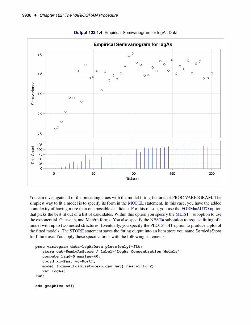
9936 F Chapter 122: The VARIOGRAM Procedure
Output 122.1.4 Empirical Semivariogram for logAs Data
You can investigate all of the preceding clues with the model fitting features of PROC VARIOGRAM. Thesimplest way to fit a model is to specify its form in the MODEL statement. In this case, you have the addedcomplexity of having more than one possible candidate. For this reason, you use the FORM=AUTO optionthat picks the best fit out of a list of candidates. Within this option you specify the MLIST= suboption to usethe exponential, Gaussian, and Matérn forms. You also specify the NEST= suboption to request fitting of amodel with up to two nested structures. Eventually, you specify the PLOTS=FIT option to produce a plot ofthe fitted models. The STORE statement saves the fitting output into an item store you name SemivAsStorefor future use. You apply these specifications with the following statements:
proc variogram data=logAsData plots(only)=fit;store out=SemivAsStore / label='LogAs Concentration Models';compute lagd=5 maxlag=40;coord xc=East yc=North;model form=auto(mlist=(exp,gau,mat) nest=1 to 2);var logAs;
run;
ods graphics off;

Example 122.1: Aspects of Semivariogram Model Fitting F 9937
The table of general information about fitting is shown in Output 122.1.5. The table lets you know that 12model combinations are to be tested for weighted least squares fitting, based on the three forms that youspecified.
Output 122.1.5 Semivariogram Model Fitting General Information
Semivariogram Model Fitting of Log-Arsenic Concentration
The VARIOGRAM Procedure
Dependent Variable: logAsAngle: Omnidirectional
Semivariogram Model Fitting of Log-Arsenic Concentration
The VARIOGRAM Procedure
Dependent Variable: logAsAngle: Omnidirectional
Semivariogram Model Fitting
Model Selection from 12 form combinations
Output Item Store WORK.SEMIVASSTORE
Item Store Label LogAs Concentration Models
The combinations include repetitions. For example, you specified the GAU form; hence the GAU-GAU formis tested, too. The model combinations also include permutations. For example, you specified the GAU andthe EXP forms; hence the GAU-EXP and EXP-GAU models are fitted separately. According to the section“Nested Models” on page 9897, it might seem that the same model is fitted twice. However, in each ofthese two cases, each structure starts the fitting process with different parameter initial values. This can leadGAU-EXP to a different fit than EXP-GAU leads to, as seen in the fitting summary table in Output 122.1.6.The table shows all the model combinations that were tested and fitted. By default, the ordering is based onthe weighted sum of squares error criterion, and you can see that the lowest values in the Weighted SSEcolumn are in top slots of the list.
Output 122.1.6 Semivariogram Model Fitting Summary
Fit Summary
Class ModelWeighted
SSE AIC
1 Gau-Gau 25.42435 -9.59246
Gau-Mat 25.42482 -7.59169
2 Exp-Gau 25.97835 -8.70865
3 Exp-Mat 26.36846 -6.09754
4 Mat 26.37519 -10.08708
5 Gau 26.78629 -11.45296
6 Exp 28.01200 -9.61851
Exp-Exp 28.01200 -5.61850
Mat-Exp 28.01200 -3.61850
Gau-Exp 28.01200 -5.61850

9938 F Chapter 122: The VARIOGRAM Procedure
Note the leftmost Class column in Output 122.1.6. As explained in detail in section “Classes of Equivalence”on page 9918, when you fit more than one model, all fitted models that compute the same semivariance areplaced in the same class of equivalence. For example, in this fitting example the top ranked GAU-GAU andGAU-MAT nested models produce indistinguishable semivariograms; for that reason they are both placed inthe same class 1 of equivalence. The same occurs with the EXP, GAU-EXP, EXP-EXP, and MAT-EXP modelsin the bottom of the table. By default, PROC VARIOGRAM uses the AIC as a secondary classificationcriterion; hence models in each equivalence class are already ordered based on their AIC values.
Another remark in Output 122.1.6 is that despite submitting 12 model combinations for fitting, the tableshows only 10. You can easily see that the combinations MAT-GAU and MAT-MAT are not among the listedmodels in the fit summary. This results from the behavior of the VARIOGRAM procedure in the followingsituation: A parameter optimization takes place during the fitting process. In the present case the optimizerkeeps increasing the Matérn smoothness parameter � in the MAT-GAU model. At the limit of an infinite �parameter, the Matérn form becomes the Gaussian form. For that reason, when the parameter � is driventowards very high values, PROC VARIOGRAM automatically replaces the Matérn form with the Gaussian.This switch converts the MAT-GAU model into a GAU-GAU model. However, a GAU-GAU model alreadyexists among the specified forms; consequently, the duplicate GAU-GAU model is skipped, and the fittedmodel list is reduced by one model. A similar explanation justifies the omission of the MAT-MAT modelfrom the fit summary table.
In our example, the nested Gaussian-Gaussian model is the fitting selection of the procedure based onthe default ranking criteria. Output 122.1.7 displays additional information about the selected model. Inparticular, you see the table with general information about the Gaussian-Gaussian model, the initial valuesused for its parameters, and information about the optimization process for the fitting.
Output 122.1.7 Fitting and Optimization Information for Gaussian-Gaussian Model
Semivariogram ModelFitting
Name Gaussian-Gaussian
Label Gau-Gau
Model Information
ParameterInitialValue
Nugget 0.0903
GauScale1 0.6709
GauRange1 100.0
GauScale2 0.6709
GauRange2 50.0230
Optimization Information
Optimization Technique Dual Quasi-Newton
Parameters in Optimization 5
Lower Boundaries 5
Upper Boundaries 0
Starting Values From PROC

Example 122.1: Aspects of Semivariogram Model Fitting F 9939
The estimated parameter values of the selected Gaussian-Gaussian model are shown in Output 122.1.8.
Output 122.1.8 Parameter Estimates of the Fitting Selected Model
Parameter Estimates
Parameter EstimateApprox
Std Error DF t ValueApproxPr > |t|
Nugget 0.08308 0.05097 36 1.63 0.1118
GauScale1 0.3277 0.2077 36 1.58 0.1234
GauRange1 62.3127 19.8488 36 3.14 0.0034
GauScale2 1.2615 0.2070 36 6.10 <.0001
GauRange2 21.4596 3.2722 36 6.56 <.0001
By default, when you specify more than one model to fit, PROC VARIOGRAM produces a fit plot thatcompares the first five classes of the successfully fit candidate models. The model that is selected accordingto the specified fitting criteria is shown with a thicker line in the plot.
You can modify the number of displayed equivalence classes with the NCLASSES= suboption of thePLOTS=FIT option. When you have such comparison plots, PROC VARIOGRAM displays the representativemodel from each class of equivalence.
The default fit plot for the current model comparison is shown in Output 122.1.9. The legend informs youthere is one more model in the first class of equivalence, as the fitting summary table indicated earlier inOutput 122.1.6.

9940 F Chapter 122: The VARIOGRAM Procedure
Output 122.1.9 Fitted Theoretical and Empirical logAs Concentration Semivariograms for the SpecifiedModels
In the present example, all fitted models in the first five classes have very similar semivariograms. Theselected Gaussian-Gaussian model seems to have a relatively larger range than the rest of the displayedmodels, but you can expect any of these models to exhibit a near-identical behavior in terms of spatialcorrelation. As a result, all models in the displayed classes are likely to lead to very similar output, if youproceed to use any of them for spatial prediction.
In that sense, semivariogram fitting is a partially subjective process, for which there might not exist only onesingle correct answer to solve your problem. In the context of the example, on one hand you might concludethat the selected Gaussian-Gaussian model is exactly sufficient to describe spatial correlation in the arsenicstudy. On the other hand, the similar performance of all models might prompt you to choose instead a moresimple non-nested model for prediction like the Matérn or the Gaussian model.
Regardless of whether you might opt to sacrifice the statistically best fit (depending on your selected criteria)to simplicity, eventually you are the one to decide which approach serves your study optimally. The modelfitting features of PROC VARIOGRAM offer you significant assistance so that you can assess your optionsefficiently.

Example 122.2: An Anisotropic Case Study with Surface Trend in the Data F 9941
Example 122.2: An Anisotropic Case Study with Surface Trend in the DataThis example shows how to examine data for nonrandom surface trends and anisotropy. You use simulateddata where the variable is atmospheric ozone (O3) concentrations measured in Dobson units (DU). Thecoordinates are offsets from a point in the southwest corner of the measurement area, with the east and northdistances in units of kilometers (km). You work with the ozoneSet data set that contains 300 measurementsin a square area of 100 km � 100 km.
The following statements read the data set:
title 'Semivariogram Analysis in Anisotropic Case With Trend Removal';
data ozoneSet;input East North Ozone @@;datalines;
34.9 68.2 286 39.2 12.5 270 44.4 37.7 275 90.5 27.0 28291.1 40.8 285 98.6 61.6 294 61.8 26.7 281 64.0 11.5 27422.4 26.5 274 89.3 18.3 279 32.3 28.3 274 31.1 53.1 27943.0 17.5 272 79.3 42.3 283 99.9 57.9 291 1.8 24.1 27381.7 73.5 294 22.9 32.0 273 64.9 67.5 292 76.5 56.3 28578.7 11.7 276 61.8 99.3 307 49.1 86.6 299 40.0 35.8 27369.3 3.8 278 23.4 9.3 270 66.3 94.3 304 71.3 6.5 2759.7 54.4 280 85.2 81.7 300 30.3 60.9 284 94.6 94.3 309
10.6 10.3 271 73.0 43.0 280 4.9 50.7 280 19.0 79.4 2892.4 73.1 287 77.7 25.2 278 8.4 27.1 276 93.5 19.7 2790.2 34.5 275 50.4 91.3 302 55.7 26.2 279 50.3 2.3 274
16.3 84.4 293 19.0 6.9 272 57.1 92.3 303 61.0 0.4 27510.7 18.7 271 15.2 43.5 277 67.0 87.4 301 79.0 54.0 28536.0 53.3 279 58.3 52.1 282 56.6 79.7 294 40.4 32.4 27548.9 64.1 286 54.0 54.9 281 27.5 48.5 279 36.4 30.3 27510.5 31.0 273 87.0 39.4 283 47.9 37.5 274 64.7 63.4 2880.5 90.8 294 22.8 22.4 275 31.1 78.8 291 93.6 49.8 2902.5 39.3 273 83.6 25.6 282 49.8 24.1 278 73.1 91.8 305
30.5 90.6 297 26.0 61.2 284 58.4 66.2 289 30.5 4.3 27338.3 85.6 298 89.2 96.6 309 53.4 6.3 275 27.3 12.8 27143.4 56.5 281 99.5 86.9 305 85.8 22.8 281 83.0 10.9 27824.8 16.7 271 51.1 18.8 275 59.0 54.3 283 35.5 91.4 29818.1 56.0 279 78.0 36.4 277 56.8 6.9 275 21.1 44.5 27773.9 75.9 296 54.2 0.1 274 33.2 75.1 290 38.2 3.3 27415.2 14.7 272 15.9 84.2 292 60.2 95.2 304 9.8 27.2 27691.2 56.4 289 94.7 86.9 303 56.7 49.6 281 24.2 9.5 27043.0 17.0 272 85.9 10.7 278 53.9 41.1 276 30.4 63.4 28662.8 86.3 299 76.8 24.6 279 31.6 94.0 300 26.9 73.8 28718.9 68.4 284 99.4 37.2 285 79.1 3.3 277 34.9 74.7 2896.4 33.8 277 48.4 82.2 294 86.0 58.0 289 92.0 60.4 293
50.2 91.6 300 12.2 38.3 275 72.7 48.9 283 82.7 34.1 27977.0 51.0 286 86.6 15.8 278 42.0 42.7 277 99.3 8.2 27817.4 70.6 286 11.2 92.4 295 60.2 28.8 280 92.0 73.3 29725.3 30.6 273 36.6 8.9 274 34.2 4.4 273 26.6 54.7 2781.7 27.4 278 49.6 1.1 275 62.8 89.3 301 28.0 49.3 279
51.2 75.1 293 59.3 93.5 304 83.6 90.5 304 79.4 87.0 30278.0 28.3 281 16.8 19.1 272 9.1 81.2 292 23.7 55.8 277

9942 F Chapter 122: The VARIOGRAM Procedure
75.5 21.3 279 64.4 43.3 279 38.9 98.9 303 22.5 87.9 29396.7 37.9 285 92.3 93.9 308 16.9 25.4 273 15.2 61.5 28373.8 94.0 306 57.4 97.2 305 73.2 4.9 276 39.2 82.3 29495.7 99.4 315 66.0 98.4 306 95.3 26.9 283 45.4 75.3 29164.8 15.4 276 69.8 55.4 284 36.3 74.9 290 9.9 22.2 27665.8 13.9 276 13.0 82.0 293 95.6 77.2 301 32.5 55.6 27945.8 35.5 275 62.2 6.6 274 25.2 51.2 279 92.4 8.1 27740.5 35.3 273 9.9 3.9 271 43.5 44.0 278 68.6 61.3 28764.2 77.5 296 57.6 81.6 294 69.5 64.7 291 64.3 95.1 3042.8 62.4 283 33.2 83.3 294 10.7 71.0 285 24.3 88.2 294
94.5 32.2 283 21.0 67.6 286 20.1 71.6 286 85.2 71.3 29694.8 30.7 283 53.4 92.0 301 81.0 50.0 287 54.6 29.9 27771.1 90.1 303 15.2 2.9 271 83.6 17.8 278 76.0 21.8 27955.6 37.4 275 86.7 83.7 303 43.6 83.6 295 44.2 31.7 27490.0 83.3 300 6.2 0.5 270 42.2 87.7 298 31.7 4.3 27391.4 41.2 285 78.0 50.6 286 27.1 56.1 278 72.6 63.9 29129.3 49.9 281 49.0 36.9 275 13.9 53.5 280 93.1 83.2 30073.0 61.6 289 63.1 27.5 280 38.3 72.5 287 72.7 34.2 2776.9 32.3 274 17.1 58.6 280 19.6 94.6 297 2.7 36.5 276
34.5 5.5 275 98.6 95.9 313 9.1 71.1 285 88.6 55.8 28726.8 78.5 289 64.8 66.6 292 59.7 25.7 280 47.3 70.2 2886.1 94.4 296 50.5 82.7 296 9.1 41.6 276 86.0 71.0 296
75.2 69.8 293 73.3 84.8 300 42.5 15.9 274 56.1 76.1 29287.9 41.2 285 65.1 9.8 274 79.0 41.2 282 44.6 65.1 28754.7 68.3 289 57.0 26.8 279 8.7 12.3 270 33.7 61.9 28625.0 55.8 278 69.3 94.9 306 49.2 64.6 287 78.2 93.7 30747.9 26.6 277 96.9 51.4 292 39.6 73.4 287 37.9 66.1 28594.5 71.4 296 51.6 18.3 276 37.6 73.2 287 68.5 10.7 27446.7 9.6 273 87.4 38.9 282 45.6 43.9 277 70.7 76.9 29682.8 53.6 287 82.5 55.4 286 37.8 5.1 275 89.8 96.1 30963.9 4.9 276 2.0 11.7 270 31.3 59.2 282 93.9 65.3 29647.9 93.0 301 29.9 36.0 274 14.6 28.3 274 17.5 70.1 2862.6 68.5 282 23.1 12.0 268 36.8 20.4 273 80.9 9.0 276
39.2 0.0 274 26.2 44.3 276 81.9 12.9 277 3.2 21.4 27276.9 76.7 297 88.6 7.7 277 9.7 8.4 273 26.7 91.5 29673.8 6.1 276 33.7 39.3 276 64.0 58.4 286 5.7 91.2 29585.8 93.8 307 85.8 39.1 281 93.9 63.4 295 53.1 46.3 27851.9 42.9 277 16.8 75.7 288 29.2 66.9 285 37.4 72.5 287;
The initial step is to explore the data set by inspecting the data spatial distribution. Run PROC VARIOGRAM,specifying the NOVARIOGRAM option in the COMPUTE statement as follows:
ods graphics on;
proc variogram data=ozoneSet;compute novariogram nhc=35;coord xc=East yc=North;var Ozone;
run;
The result is a scatter plot of the observed data shown in Output 122.2.1. The scatter plot suggests an almostuniform spread of the measurements throughout the prediction area. No direct inference can be made aboutthe existence of a surface trend in the data. However, the apparent stratification of ozone values in thenortheast–southwest direction might indicate a nonrandom trend.

Example 122.2: An Anisotropic Case Study with Surface Trend in the Data F 9943
Output 122.2.1 Ozone Observation Data Scatter Plot
You need to define the size and count of the data classes by specifying suitable values for the LAGDIS-TANCE= and MAXLAGS= options, respectively. Compared to the smaller sample of thickness data usedin “Getting Started: VARIOGRAM Procedure” on page 9847, the larger size of the ozoneSet data resultsin more densely populated distance classes for the same value of the NHCLASSES= option. After youexperiment with a variety of values for the NHCLASSES= option, you can adjust LAGDISTANCE= tohave a relatively small number. Then you can account for a large value of MAXLAGS= so that you obtainmany sample semivariogram points within your data correlation range. Specifying these values requiressome exploration, for which you might need to return to this point from a later stage in your semivariogramanalysis. For illustration purposes you now specify NHCLASSES=35.
Your choice of NHCLASSES=35 yields the pairwise distance intervals table in Output 122.2.2 and thecorresponding histogram in Output 122.2.3.

9944 F Chapter 122: The VARIOGRAM Procedure
Output 122.2.2 Pairwise Distance Intervals Table
Pairwise Distance Intervals
LagClass Bounds
Numberof Pairs
Percentageof Pairs
0 0.00 2.01 52 0.12%
1 2.01 6.03 420 0.94%
2 6.03 10.06 815 1.82%
3 10.06 14.08 1143 2.55%
4 14.08 18.10 1518 3.38%
5 18.10 22.12 1680 3.75%
6 22.12 26.15 1931 4.31%
7 26.15 30.17 2135 4.76%
8 30.17 34.19 2285 5.09%
9 34.19 38.21 2408 5.37%
10 38.21 42.24 2551 5.69%
11 42.24 46.26 2444 5.45%
12 46.26 50.28 2535 5.65%
13 50.28 54.30 2487 5.55%
14 54.30 58.33 2460 5.48%
15 58.33 62.35 2391 5.33%
16 62.35 66.37 2302 5.13%
17 66.37 70.39 2285 5.09%
18 70.39 74.41 2079 4.64%
19 74.41 78.44 1786 3.98%
20 78.44 82.46 1640 3.66%
21 82.46 86.48 1493 3.33%
22 86.48 90.50 1243 2.77%
23 90.50 94.53 925 2.06%
24 94.53 98.55 710 1.58%
25 98.55 102.57 421 0.94%
26 102.57 106.59 274 0.61%
27 106.59 110.62 200 0.45%
28 110.62 114.64 120 0.27%
29 114.64 118.66 55 0.12%
30 118.66 122.68 35 0.08%
31 122.68 126.71 14 0.03%
32 126.71 130.73 11 0.02%
33 130.73 134.75 2 0.00%
34 134.75 138.77 0 0.00%
35 138.77 142.80 0 0.00%
Notice the overall high pair count in the majority of classes in Output 122.2.2. You can see that even forhigher values of NHCLASSES= the classes are still sufficiently populated for your semivariogram analysisaccording to the rule of thumb stated in the section “Choosing the Size of Classes” on page 9907. Based onthe displayed information in Output 122.2.3, you specify LAGDISTANCE=4 km. You can further experimentwith smaller lag sizes to obtain more points in your sample semivariogram.

Example 122.2: An Anisotropic Case Study with Surface Trend in the Data F 9945
You can focus on the MAXLAGS= specification at a later point. The important step now is to investigatethe presence of trends in the measurement. The following section makes a suggestion about how to removesurface trends from your data and then continues the semivariogram analysis with the detrended data.
Output 122.2.3 Distribution of Pairwise Distances for Ozone Observation Data
Analysis with Surface Trend Removal
You can use a SAS/STAT predictive modeling procedure to extract surface trends from your original data. Ifyour goal is spatial prediction, you can continue processing the detrended data for the prediction tasks, and atthe end you can reinstate the trend at the prediction locations to report your analysis results.
In general, the exact form of the trend is unknown, as discussed in the section “Empirical Semivariogramsand Surface Trends” on page 9910. In this case, the spatial distribution of the measurements shown inFigure 122.2.1 suggests that you can use a quadratic model to describe the surface trend like the one thatfollows:
T .East;North/ D f0 C f1 ŒEast�C f2 ŒEast�2 C f3 ŒNorth�C f4 ŒNorth�2

9946 F Chapter 122: The VARIOGRAM Procedure
The following statements show how to invoke the GLM procedure for your ozone data and how to extract thepreceding trend from them:
proc glm data=ozoneSet plots=none;model ozone = East East*East North North*North;output out=gmout predicted=pred residual=ResidualOzone;
run;
Among other output, PROC GLM produces estimates for the parameters f0; : : : ; f4 in the preceding trendmodel. Output 122.2.4 shows the table with the parameter estimates. In this table, the coefficient f0corresponds to the intercept estimate, and the rest of the coefficients correspond to their matching variables;for example, the estimate in the line of “East*East” refers to f2 in the preceding model. For more informationabout the syntax and the PROC GLM output, see Chapter 46, “The GLM Procedure.”
Output 122.2.4 Parameter Estimates for the Surface Trend Model
Semivariogram Analysis in Anisotropic Case With Trend Removal
The GLM Procedure
Dependent Variable: Ozone
Semivariogram Analysis in Anisotropic Case With Trend Removal
The GLM Procedure
Dependent Variable: Ozone
Parameter EstimateStandard
Error t Value Pr > |t|
Intercept 270.6798273 0.40595731 666.77 <.0001
East 0.0065148 0.01360281 0.48 0.6323
East*East 0.0010726 0.00012987 8.26 <.0001
North -0.0369159 0.01297491 -2.85 0.0047
North*North 0.0035587 0.00012659 28.11 <.0001
The detrending process leaves you with the GMOUT data set, which contains the ResidualOzone dataresiduals. This time you run PROC VARIOGRAM again with the NOVARIOGRAM option to inspect thedetrended residuals, and with a request only for the observations plot, as follows:
proc variogram data=gmout plots(only)=observ;compute novariogram nhc=35;coord xc=East yc=North;var ResidualOzone;
run;
The requested observations plot is shown in Output 122.2.5.

Example 122.2: An Anisotropic Case Study with Surface Trend in the Data F 9947
Output 122.2.5 Ozone Residual Observation Data Scatter Plot
Before you proceed with the empirical semivariogram computation and model fitting, examine your datafor anisotropy. This investigation is necessary to portray the spatial structure of your SRF accurately. Ifanisotropy exists, it manifests itself as different ranges or sills or both for the empirical semivariograms indifferent directions.
You want detail in your analysis, so you ask for the empirical semivariance in 12 directions by specifyingNDIRECTIONS=12. Based on the NDIRECTIONS= option, empirical semivariograms are produced inincrements of the base angle � D 180ı=12 D 15ı.
You also choose ANGLETOLERANCE=22.5 and BANDWIDTH=20. A different choice of values producesdifferent empirical semivariograms, because these options can regulate the number of pairs that are includedin a class. Avoid assigning values that are too small to these parameters so that you can allow for an adequatenumber of point pairs per class. At the same time, the higher the values of these parameters are, the moredata pairs that come from closely neighboring directions are included in each lag. Therefore, values for theANGLETOLERANCE= and BANDWIDTH= options that are too high pose a risk of losing information alongthe particular direction. The side effect occurs because you incorporate data pairs from a broader spectrumof angles; thus, you potentially amplify weaker anisotropy or weaken stronger anisotropy, as noted in thesection “Angle Classification” on page 9902. You can experiment with different ANGLETOLERANCE=and BANDWIDTH= values to reach this balance with your data, if necessary.

9948 F Chapter 122: The VARIOGRAM Procedure
With the following statements you ask to display only the SEMIVAR plots in the specified number ofdirections. Multiple empirical semivariograms are placed by default in panels, as Output 122.2.6 shows. If youwant an individual plot for each angle, then you need to further specify the plot option SEMIVAR(UNPACK).
proc variogram data=gmout plot(only)=semivar;compute lagd=4 maxlag=16 ndir=12 atol=22.5 bandw=20;coord xc=East yc=North;var ResidualOzone;
run;
Output 122.2.6 Ozone Empirical Semivariograms with 0ı � � < 180ı and ı� D 15ı

Example 122.2: An Anisotropic Case Study with Surface Trend in the Data F 9949
Output 122.2.6 continued
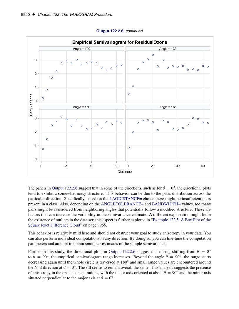
9950 F Chapter 122: The VARIOGRAM Procedure
Output 122.2.6 continued
The panels in Output 122.2.6 suggest that in some of the directions, such as for � D 0ı, the directional plotstend to exhibit a somewhat noisy structure. This behavior can be due to the pairs distribution across theparticular direction. Specifically, based on the LAGDISTANCE= choice there might be insufficient pairspresent in a class. Also, depending on the ANGLETOLERANCE= and BANDWIDTH= values, too manypairs might be considered from neighboring angles that potentially follow a modified structure. These arefactors that can increase the variability in the semivariance estimate. A different explanation might lie inthe existence of outliers in the data set; this aspect is further explored in “Example 122.5: A Box Plot of theSquare Root Difference Cloud” on page 9966.
This behavior is relatively mild here and should not obstruct your goal to study anisotropy in your data. Youcan also perform individual computations in any direction. By doing so, you can fine-tune the computationparameters and attempt to obtain smoother estimates of the sample semivariance.
Further in this study, the directional plots in Output 122.2.6 suggest that during shifting from � D 0ı
to � D 90ı, the empirical semivariogram range increases. Beyond the angle � D 90ı, the range startsdecreasing again until the whole circle is traversed at 180ı and small range values are encountered aroundthe N–S direction at � D 0ı. The sill seems to remain overall the same. This analysis suggests the presenceof anisotropy in the ozone concentrations, with the major axis oriented at about � D 90ı and the minor axissituated perpendicular to the major axis at � D 0ı.

Example 122.2: An Anisotropic Case Study with Surface Trend in the Data F 9951
The multidirectional analysis requires that for a given LAGDISTANCE= you also specify a MAXLAGS=value. Since the ozone correlation range might be unknown (as assumed here), you can apply the rule ofthumb that suggests use of the half-extreme data distance in the direction of interest, as explained in thesection “Spatial Extent of the Empirical Semivariogram” on page 9908. Following the information displayedin Output 122.2.3, for different directions this distance varies between 99:4=2 D 49:7 and 140:8=2 D 70:4km. In turn, the pairwise distances table in Output 122.2.2 indicates that within this range of distances youcan specify MAXLAGS= to be between 12 and 17 lags. In this example you specify MAXLAGS=16.
At this point you are ready to continue with fitting theoretical semivariogram models to the empiricalsemivariogram in the selected directions of � D 0ı and � D 90ı. By trying out different models, you seethat an exponential one is suitable for your empirical data:
z.h/ D c0
�1 � exp
��h
a0
��
For the purpose of the present example, it is reasonable to assume a constant nugget effect equal to zero,based on the empirical semivariograms shown in Output 122.2.6. The same output suggests that the modelscale is likely to be above 2, and that the range might be relatively small in � D 0ı. You specify the PARMSstatement to set initial values for the exponential model parameters and account for these considerations.
In particular, you assign an initial value of zero to the nugget effect. Then you request a grid search for therange and scale parameters, so that the optimal initial values set is selected for the parameter estimation ineach of the two angles � D 0ı and � D 90ı. By inspecting the empirical semivariograms in Output 122.2.6,you specify the value list 2, 2.5, and 3 for the scale, and the values from 5 to 25 with a step of 10 for therange. In addition, you specify the parameter 1 in the HOLD= option to designate the nugget effect parameteras a constant. According to these specifications, you use the following statements:
proc variogram data=gmout plot(only)=fit;compute lagd=4 maxlag=16;directions 0(22.5,10) 90(22.5,10);coord xc=East yc=North;model form=exp;parms (0.) (2 to 3 by 0.5) (5 to 25 by 10) / hold=(1);var ResidualOzone;
run;
ods graphics off;
The VARIOGRAM procedure repeats the fitting process for each one of the selected directions. First, in� D 0ı the parameter search table in Output 122.2.7 shows you which value combinations are tested initiallyto choose the one that gives the lowest objective function value.

9952 F Chapter 122: The VARIOGRAM Procedure
Output 122.2.7 Parameter Search for the Selected Direction � D 0ı
Semivariogram Analysis in Anisotropic Case With Trend Removal
The VARIOGRAM Procedure
Dependent Variable: ResidualOzoneAngle: 0
Current Model: Exponential
Semivariogram Analysis in Anisotropic Case With Trend Removal
The VARIOGRAM Procedure
Dependent Variable: ResidualOzoneAngle: 0
Current Model: Exponential
Parameter Search
Set Nugget Scale RangeObjectiveFunction
1 0 2 5 391.06593
2 0 2 15 1740.0
3 0 2 25 5167.5
4 0 2.5 5 64.86565
5 0 2.5 15 664.03665
6 0 2.5 25 2480.5
7 0 3 5 72.86743
8 0 3 15 305.53306
9 0 3 25 1305.0
From this search, the combination of scale equal to 2.5 and a range of size 5 is passed as initial values to themodel fitting process. This result is reflected in the model information table shown in Output 122.2.8.
Output 122.2.8 Model Initial Values for the Selected Direction � D 0ı
Model Information
ParameterInitialValue Status
Nugget 0 Fixed
Scale 2.5000
Range 5.0000
Fitting is successful, and among the output objects you can see the estimated parameters and the fit summarytables for the direction � D 0ı in Output 122.2.9.
Output 122.2.9 Weighted Least Squares Fitting Parameter Estimates and Summary for the SelectedDirection � D 0ı
Parameter Estimates
Parameter EstimateApprox
Std Error DF t ValueApproxPr > |t|
Scale 2.6657 0.03830 15 69.60 <.0001
Range 3.7277 0.5609 15 6.65 <.0001
Fit Summary
ModelWeighted
SSE AIC
Exp 43.35103 19.91399

Example 122.2: An Anisotropic Case Study with Surface Trend in the Data F 9953
A corresponding parameter search takes place for the direction � D 90ı. The respective table and the choiceof initial values for fitting in the direction � D 90ı are shown in Output 122.2.10.
Output 122.2.10 Parameter Search and Model Initial Values for the Selected Direction � D 90ı
Parameter Search
Set Nugget Scale RangeObjectiveFunction
1 0 2 5 302.54551
2 0 2 15 635.93338
3 0 2 25 1996.0
4 0 2.5 5 95.09939
5 0 2.5 15 104.56776
6 0 2.5 25 662.06813
7 0 3 5 155.50670
8 0 3 15 20.48482
9 0 3 25 190.30599
Model Information
ParameterInitialValue Status
Nugget 0 Fixed
Scale 3.0000
Range 15.0000
Output 122.2.11 displays the estimated parameters and the fit summary for the direction � D 90ı.
Output 122.2.11 Weighted Least Squares Fitting Parameter Estimates and Summary for the SelectedDirection � D 90ı
Parameter Estimates
Parameter EstimateApprox
Std Error DF t ValueApproxPr > |t|
Scale 2.9199 0.07007 15 41.67 <.0001
Range 14.7576 0.9530 15 15.49 <.0001
Fit Summary
ModelWeighted
SSE AIC
Exp 19.12246 6.00005
The fitted and empirical semivariograms for the selected directions are displayed in the panel of Out-put 122.2.12.

9954 F Chapter 122: The VARIOGRAM Procedure
Output 122.2.12 Fitted Theoretical and Empirical Semivariogram for the Ozone Data in the � D 0ı and� D 90ı Directions
Conclusively, your semivariogram analysis on the detrended ozone data suggests that the ozone SRF exhibitsanisotropy in the perpendicular directions of N–S (� D 0ı) and E–W (� D 90ı).
The sills in the two directions of anisotropy are similar in size. By inspecting again the empirical semivar-iograms in Output 122.2.6, you could make the reasonable assumption that you have a case of geometricanisotropy, where the range in the major axis is about 4.5 times larger than the minor axis range. If youwould like to use these PROC VARIOGRAM results for predictions, then you would need to specify a singlescale value for the geometric anisotropy sill. In this case you could choose an arbitrary value for the constantscale from the narrow interval formed by the estimated scales in the previous results. For example, you canspecify the PARMS statement modified as shown in the following statement to approximate a common scalefor the semivariance in all directions:
parms (0.) (2.7) (5 to 25 by 10) / hold=(1,2);
As an alternative, you can use PROC VARIOGRAM to fit an exponential model to all different anglesexamined in this example, and then select the constant scale value to be the mean of the scales across alldirections.

Example 122.3: Analysis without Surface Trend Removal F 9955
Example 122.3: Analysis without Surface Trend RemovalThis example uses PROC VARIOGRAM without removing potential surface trends in a data set in orderto investigate a distinguished spatial direction in the data. In doing so, this example also serves as aguide to examine under which circumstances you might be able to bypass the effect of a trend on asemivariogram. Typically though, for theoretical semivariogram estimations you follow the analysis presentedin “Example 122.2: An Anisotropic Case Study with Surface Trend in the Data” on page 9941.
As explained in the section “Details: VARIOGRAM Procedure” on page 9892, when you compute the empir-ical semivariance for data that contain underlying surface trends, the outcome is the pseudo-semivariance.Pseudo-semivariograms are not estimates of the theoretical semivariogram; hence, they provide no informa-tion about the spatial continuity of your SRF.
However, in the section “Empirical Semivariograms and Surface Trends” on page 9910 it is mentioned thatyou might still be able to perform a semivariogram analysis with potentially non-trend-free data, if yoususpect that your measurements might be trend-free across one or more specific directions. The exampledemonstrates this approach.
Reconsider the ozone data presented at the beginning of “Example 122.2: An Anisotropic Case Study withSurface Trend in the Data” on page 9941. The spatial distribution of the data is shown in Figure 122.2.1,and the pairwise distance distribution for NHCLASSES=35 is illustrated in Figure 122.2.3. This exploratoryanalysis suggested a LAGDISTANCE=4 km, and Figure 122.2.2 indicated that for this LAGDISTANCE=you can consider a value of MAXLAGS=16.
Recall from the section “Empirical Semivariograms and Surface Trends” on page 9910 that you need toinvestigate the empirical semivariogram of the data in a few different directions in order to identify a trend-freedirection. If such a direction exists, then you can proceed with this special type of analysis. The followingstatements employ NDIRECTIONS=8 to examine eight directions:
ods graphics on;
proc variogram data=ozoneSet plot(only)=semivar;compute lagd=4 maxlag=16 ndirections=8 robust;coord xc=East yc=North;var Ozone;
run;
By default, the range of 180ı is divided into eight equally distanced angles: � D 0ı, � D 22:5ı, � D 45ı,� D 67:5ı, � D 90ı, � D 112:5ı, � D 135ı, and � D 157:5ı. The resulting empirical semivariograms forthese angles are shown in Output 122.3.1.

9956 F Chapter 122: The VARIOGRAM Procedure
Output 122.3.1 Ozone Empirical Semivariograms with 0ı � � < 180ı and ı� D 22:5ı

Example 122.3: Analysis without Surface Trend Removal F 9957
Output 122.3.1 continued
The figures in Output 122.3.1 suggest an overall continuing increase with distance of the semivariance in alldirections. As explained in the section “Theoretical Semivariogram Models” on page 9892, this can be anindication of systematic trends in the data. However, the direction of � D 112:5ı clearly indicates that theincrease rate, if any, is smaller than the corresponding rates across the rest of the directions. You then want tosearch whether there exists a trend-free direction in the neighborhood of this angle.
Run PROC VARIOGRAM again, specifying several directions within an interval of angles where youwant to close in and you suspect the existence of a trend-free direction. In the following step youspecify ANGLETOL=15ı, which is smaller than the default value of 22.5ı, and you also specifyBANDWIDTH=10 km. The smaller values help with minimization of the interference with neighboringdirections, as discussed in the section “Angle Classification” on page 9902.
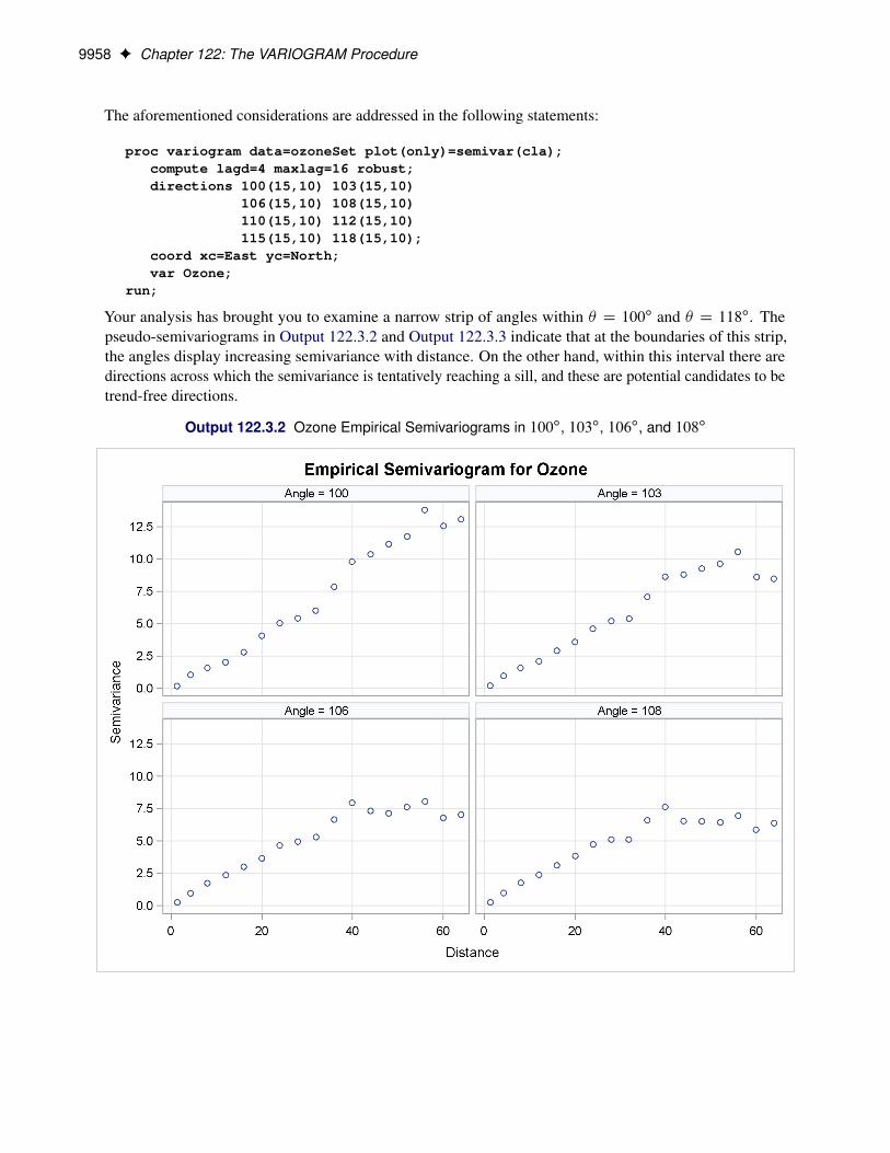
9958 F Chapter 122: The VARIOGRAM Procedure
The aforementioned considerations are addressed in the following statements:
proc variogram data=ozoneSet plot(only)=semivar(cla);compute lagd=4 maxlag=16 robust;directions 100(15,10) 103(15,10)
106(15,10) 108(15,10)110(15,10) 112(15,10)115(15,10) 118(15,10);
coord xc=East yc=North;var Ozone;
run;
Your analysis has brought you to examine a narrow strip of angles within � D 100ı and � D 118ı. Thepseudo-semivariograms in Output 122.3.2 and Output 122.3.3 indicate that at the boundaries of this strip,the angles display increasing semivariance with distance. On the other hand, within this interval there aredirections across which the semivariance is tentatively reaching a sill, and these are potential candidates to betrend-free directions.
Output 122.3.2 Ozone Empirical Semivariograms in 100ı, 103ı, 106ı, and 108ı

Example 122.3: Analysis without Surface Trend Removal F 9959
Output 122.3.3 Ozone Empirical Semivariograms in 110ı, 112ı, 115ı, and 118ı
You can further investigate this angle spectrum in more detail. For example, you can monitor additionalangles in between, or use a smaller LAGDISTANCE= and increased MAXLAGS= values to single out themost qualified candidate. For the purpose of this example, you can consider the direction � D 108ı to verylikely be the trend-free one you are looking for.
From a physical standpoint, the trend-free direction, if it exists, is expected to be perpendicular to the directionof the maximum dip in the values of the ozone field, as mentioned in the section “Empirical Semivariogramsand Surface Trends” on page 9910. If you cross-examine the ozone data distribution in Output 122.2.1,the figure suggests that this direction exists and is slightly tilted clockwise with respect to the E–W axis.This direction emerges from the mild stratification of the ozone values in your data distribution. The ozoneconcentrations across it are similar when compared to surrounding directions, and as such, it has beenidentified as a trend-free direction.
Your next step is to obtain the empirical semivariogram in the suspected trend-free direction of � D 108ı andto perform a theoretical model fit.
The semivariance in Output 122.3.2 exhibits a slow, almost linear rise at short distances and seems to bereaching the sill fast, rather than asymptotically. You can accommodate this behavior by using the sphericalmodel
z.h/ D
(cn C �0
2h32ha0�12. ha0/3i; for 0 < h � a0
c0; for a0 < h
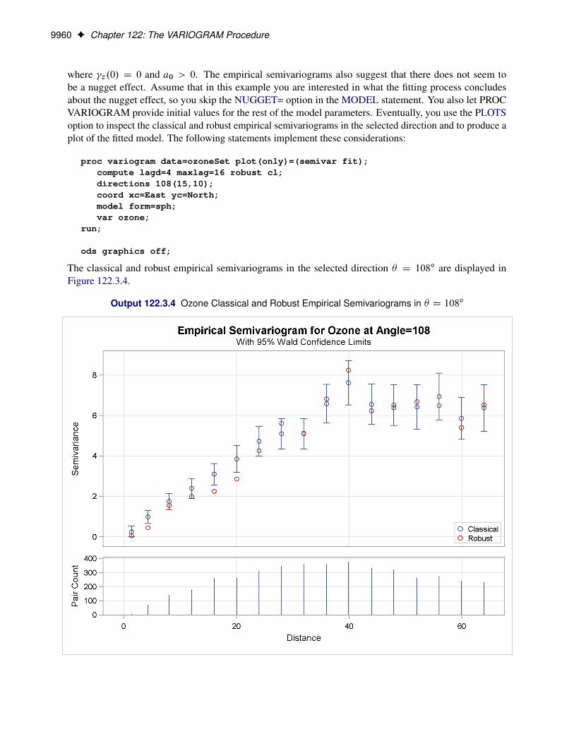
9960 F Chapter 122: The VARIOGRAM Procedure
where z.0/ D 0 and a0 > 0. The empirical semivariograms also suggest that there does not seem tobe a nugget effect. Assume that in this example you are interested in what the fitting process concludesabout the nugget effect, so you skip the NUGGET= option in the MODEL statement. You also let PROCVARIOGRAM provide initial values for the rest of the model parameters. Eventually, you use the PLOTSoption to inspect the classical and robust empirical semivariograms in the selected direction and to produce aplot of the fitted model. The following statements implement these considerations:
proc variogram data=ozoneSet plot(only)=(semivar fit);compute lagd=4 maxlag=16 robust cl;directions 108(15,10);coord xc=East yc=North;model form=sph;var ozone;
run;
ods graphics off;
The classical and robust empirical semivariograms in the selected direction � D 108ı are displayed inFigure 122.3.4.
Output 122.3.4 Ozone Classical and Robust Empirical Semivariograms in � D 108ı

Example 122.3: Analysis without Surface Trend Removal F 9961
The output continues with information about the fitting process, which terminates successfully and producesthe estimated parameters and the fit summary tables shown in Output 122.3.5. The near-zero nugget parameterestimate indicates that you can consider the process to be practically free of nugget effect.
Output 122.3.5 Weighted Least Squares Fitting Parameter Estimates and Summary in � D 108ı
Parameter Estimates
Parameter EstimateApprox
Std Error DF t ValueApproxPr > |t|
Nugget 0.006260 0.09449 14 0.07 0.9481
Scale 6.6791 0.1741 14 38.37 <.0001
Range 47.3012 2.0776 14 22.77 <.0001
Fit Summary
ModelWeighted
SSE AIC
Sph 13.13869 1.61991
The fitted and empirical semivariograms for the selected direction � D 108ı are displayed in Output 122.3.6.
Output 122.3.6 Fitted Theoretical and Empirical Semivariogram for the Ozone Data in � D 108ı

9962 F Chapter 122: The VARIOGRAM Procedure
A comparative look at the empirical and fitted semivariograms in Output 122.3.6 and Output 122.2.12suggests that the analysis of the trend-free ResidualOzone produces a different outcome from that of theoriginal Ozone values. In fact, a more suitable comparison can be made between the semivariograms in theassumed trend-free direction � D 108ı of the current scenario and the one shown in Output 122.2.6 in thenearly identical direction � D 105ı. It might seem unreasonable that these two semivariograms are producedboth in the same ozone study and in a narrow band of directions free of apparent surface trends, yet they bearno resemblance. However, the lack of similarity in these plots stems from operating on two different data setswhere the outcome depends on the actual data values.
More specifically, the semivariogram analysis treats the trend-free ozone set and the original ozone measure-ments as different quantities. The process of detrending the original Ozone values is a transformation ofthese values into the trend-free values of ResidualOzone. Any existing spatial correlation in the originaldata is not necessarily retained within the transformed data. Depending on the transformation features, theemerging data set has its own characteristics, as demonstrated in this example.
A final remark concerns the issue of isotropy. Based on the details presented in the section “EmpiricalSemivariograms and Surface Trends” on page 9910, your knowledge of the spatial structure of the ozoneSetdata set is limited to the selected trend-free direction you indicated in the present example. You can generalizethis outcome for all spatial directions only if you consider the hypothesis of isotropy in the ozone field to bereasonable. However, you cannot infer the assumption of anisotropy in the present example based on theanalysis in the section “Analysis with Surface Trend Removal” on page 9945. Again, the reason is that youcurrently use the observed Ozone values, whereas the ResidualOzone data in the previous example emergedfrom a transformation of the current data. Hence, you have essentially two data sets that do not necessarilyshare the same properties.
Example 122.4: Covariogram and SemivariogramThe covariance that was reviewed in the section “Stationarity” on page 9899 is an alternative measureof spatial continuity that can be used instead of the semivariance. In a similar manner to the empiricalsemivariance that was presented in the section “Theoretical and Computational Details of the Semivariogram”on page 9897, you can also compute the empirical covariance. The covariograms are plots of this quantityand can be used to fit permissible theoretical covariance models, in correspondence to the semivariogramanalysis presented in the section “Theoretical Semivariogram Models” on page 9892. This example displaysa comparative view of the empirical covariogram and semivariogram, and examines some additional aspectsof these two measures.
You consider 500 simulations of an SRF Z.s/ in a square domain of 100 � 100 (106 km2). The followingDATA step defines the data locations:
title 'Covariogram and Semivariogram';
data dataCoord;retain seed 837591;do i=1 to 100;
East = round(100*ranuni(seed),0.1);North = round(100*ranuni(seed),0.1);output;
end;run;

Example 122.4: Covariogram and Semivariogram F 9963
For the simulations you use PROC SIM2D, which produces Gaussian simulations of SRFs with user-specifiedcovariance structure—see Chapter 103, “The SIM2D Procedure.” The Gaussian SRF implies full knowledgeof the SRF expected value EŒZ.s/� and variance VarŒZ.s/� at every location s. The following statementssimulate an isotropic, second-order stationary SRF with constant expected value and variance throughout thesimulation domain:
proc sim2d outsim=dataSims;simulate numreal=500 seed=79750
nugget=2 scale=6 range=10 form=exp;mean 30;grid gdata=dataCoord xc=East yc=North;
run;
Here, the SIMULATE statement accommodates the simulation parameters. The NUMREAL= option specifiesthat you want to perform 500 simulations, and the SEED= option specifies the seed for the simulation randomnumber generator. You use the MEAN statement to specify the expected value EŒZ.s/� D 30 units of Z. Youalso specify two variance components. The first is the nugget effect, and you use the NUGGET= optionto set it to cn D 2. The second is the partial sill �02 D 6 that you specify with the SCALE= option. Thetwo variance components make up the total SRF variance VarŒZ.s/� D cn C �0
2 D 8. You assume anexponential covariance structure to describe the field spatial continuity, where �02 is the sill value and itsrange a0 D 10 km (effective range a� D 3a0 D 30 km) is specified by the RANGE= option. The optionFORM= specifies the covariance structure type.
The empirical semivariance and covariance are computed by the VARIOGRAM procedure, and are availableeither in the ODS output semivariogram table (as variables Semivariance and Covariance, respectively) or inthe OUTVAR= data set. In the following statements you obtain these variables by using the OUTVAR= dataset of the VARIOGRAM procedure:
proc variogram data=dataSims outv=outv noprint;compute lagd=3 maxlag=18;coord xc=gxc yc=gyc;by _ITER_;var svalue;
run;
For each distance lag you take the average of the empirical measures over the number of simulations. PROCSORT prepares the input data for PROC MEANS, which produces these averages and stores them in thedataAvgs data set. This sequence is performed with the following statements:
proc sort data=outv;by lag;
run;
proc means data=outv n mean noprint;var Distance variog covar;by lag;output out=dataAvgs mean(variog)=Semivariance
mean(covar)=Covariancemean(Distance)=Distance;
run;
The SGPLOT procedure creates the plot of the average empirical semivariogram and covariogram, as in thefollowing statements:
9964 F Chapter 122: The VARIOGRAM Procedure
proc sgplot data=dataAvgs;title "Empirical Semivariogram and Covariogram";xaxis label = "Distance" grid;yaxis label = "Semivariance" min=-0.5 max=9 grid;y2axis label = "Covariance" min=-0.5 max=9;scatter y=Semivariance x=Distance /
markerattrs = GraphData1name='Semivar'legendlabel='Semivariance';
scatter y=Covariance x=Distance /y2axismarkerattrs = GraphData2name='Covar'legendlabel='Covariance';
discretelegend 'Semivar' 'Covar';run;
The plot of the average empirical semivariance and covariance of the preceding analysis is shown inOutput 122.4.1. The high number of simulations led to averages of empirical continuity measures thataccurately approximate the simulated SRF characteristics. Specifically, the empirical semivariogram andcovariogram both exhibit clearly exponential behavior. The semivariogram sill is approximately at thespecified variance VarŒZ.s/� D 8 of the SRF.
The simulated SRF is second-order stationary, so you expect at each lag the sum of the empirical semivarianceand covariance to approximate the field variance VarŒZ.s/�, as explained in the section “Stationarity” onpage 9899. This behavior is evident in Output 122.4.1.
This example concludes with a discussion of basic reasons why the empirical semivariogram analysis iscommonly preferred to the empirical covariance analysis. A first reason comes from the assumptions that arenecessary to compute each of these two measures. The condition of intrinsic stationarity that is required inorder to define the empirical semivariogram is less restrictive than the condition of second-order stationaritythat is required in order to consider the covariance function as a parameter of the process.
Also, an empirical semivariogram can indicate whether a nugget effect is present in your data sample, whereasthe empirical covariogram itself might not reveal this information. This point is illustrated in Output 122.4.1,where you expect to see that C.0/ D VarŒZ.s/�, but the empirical covariogram cannot have a point at exactlyh D 0. A practical way to investigate for a nugget effect when you use empirical covariograms is as follows:recall that the OUTVAR= data set provides you with the sample variance (shown in the COVAR column forLAG=–1), as the following statement shows:
/* Obtain the sample variance from the data set ----------------*/
proc print data=dataAvgs (obs=1);run;

Example 122.4: Covariogram and Semivariogram F 9965
Output 122.4.1 Average Empirical Semivariogram and Covariogram from 500 Simulations
Output 122.4.2 is a partial output of the dataAvgs data set, which contains averages of the OUTVAR= dataset and shows the computed average C.0/ in the Covariance column. The combination of the empiricalcovariogram and the C.0/ value can help you fit a theoretical covariance model that includes any nuggeteffect, if present. See also the discussion in Schabenberger and Gotway (2005, section 4.2.2) about theMatérn definition of the covariance function that is related to this issue. In particular, this definition providesfor an additional variance component in the covariance expression at h D 0 to account for the correspondingnugget effect in the semivariogram.
Output 122.4.2 Partial Outcome of the dataAvgs Data Set
Empirical Semivariogram and CovariogramEmpirical Semivariogram and Covariogram
Obs LAG _TYPE_ _FREQ_ Semivariance Covariance Distance
1 -1 0 500 . 7.74832 .
In addition to the preceding points, if the SRF is nonstationary, the empirical semivariogram indicates thatthe SRF variance increases with distance h, as Output 122.3.1 shows in “Example 122.3: Analysis withoutSurface Trend Removal” on page 9955. In that case it makes no sense to compute the empirical covariogram.

9966 F Chapter 122: The VARIOGRAM Procedure
Specifically, the covariogram could provide you with an estimate of the sample variance, which is notsufficient to indicate that the SRF might not be stationary (see also Chilès and Delfiner 1999, p. 31).
Finally, the definitions of the empirical semivariance and covariance in the section “Theoretical and Com-putational Details of the Semivariogram” on page 9897 clearly show that the sample mean NZ and the SRFexpected value EŒZ.s/� are not important for the computation of the semivariance, but either one is necessaryfor the covariance. Hence, the semivariance expression filters the mean, and this behavior is especiallyuseful when the mean is unknown. On the other hand, if EŒZ.s/� is unknown and the empirical covariance iscomputed based on the sample mean NZ, this can induce additional bias in the covariance computation.
Example 122.5: A Box Plot of the Square Root Difference CloudThe Gaussian form selected for the semivariogram in the section “Getting Started: VARIOGRAM Procedure”on page 9847 is based on consideration of the plots of the sample semivariogram. For the coal thickness data,the Gaussian form appears to be a reasonable choice.
However, it can often happen that a plot of the sample variogram shows so much scatter that no particularform is evident. The cause of this scatter can be one or more outliers in the pairwise differences of themeasured quantities.
A method of identifying potential outliers is discussed in Cressie (1993, section 2.2.2). This exampleillustrates how to use the OUTPAIR= data set from PROC VARIOGRAM to produce a square root differencecloud, which is useful in detecting outliers.
For the SRF Z.s/; s 2 R2, the square root difference cloud for a particular direction e is given by
j Z.si C he/ �Z.si / j12
for a given lag distance h. In the actual computation, all pairs P1P2 of points P1, P2 within a distancetolerance around h and an angle tolerance around the direction e are used. This generates a number of pointpairs for each lag class h. The spread of these values gives an indication of outliers.
Following the example in the section “Getting Started: VARIOGRAM Procedure” on page 9847, this exampleuses a basic LAGDISTANCE=7, with a distance tolerance of 3.5, and a direction of N–S, with an angletolerance ATOL=30ı.
First, use PROC VARIOGRAM to produce an OUTPAIR= data set. Then use a DATA step to subset this databy choosing pairs within 30ı of N–S. In addition, compute lag class and square root difference variables, asthe following statements show:
title 'Square Root Difference Cloud Example';
proc variogram data=sashelp.thick outp=outp noprint;compute novariogram;coordinates xc=East yc=North;var Thick;
run;

Example 122.5: A Box Plot of the Square Root Difference Cloud F 9967
data sqroot;set outp;/*- Include only points +/- 30 degrees of N-S -------*/where abs(cos) < 0.5;/*- Unit lag of 7, distance tolerance of 3.5 --------*/lag_class=int(distance/7 + 0.5000001);sqr_diff=sqrt(abs(v1-v2));
run;
proc sort data=sqroot;by lag_class;
run;
Next, summarize the results by using the MEANS procedure:
proc means data=sqroot noprint n mean std;var sqr_diff;by lag_class;output out=msqrt n=n mean=mean std=std;
run;title2 'Summary of Results';
proc print data=msqrt;id lag_class;var n mean std;
run;
The preceding statements produce Output 122.5.1.
Output 122.5.1 Summary of Results
Square Root Difference Cloud ExampleSummary of Results
Square Root Difference Cloud ExampleSummary of Results
lag_class n mean std
0 5 0.47300 0.14263
1 31 0.77338 0.41467
2 51 1.17052 0.47800
3 58 1.52287 0.51454
4 65 1.68625 0.58465
5 65 1.66963 0.68582
6 80 1.79693 0.62929
7 88 1.73334 0.73191
8 83 1.75528 0.68767
9 108 1.72901 0.58274
10 80 1.48268 0.48695
11 84 1.19242 0.47037
12 68 0.89765 0.42510
13 38 0.84223 0.44249
14 7 1.05653 0.42548
15 3 1.35076 0.11472
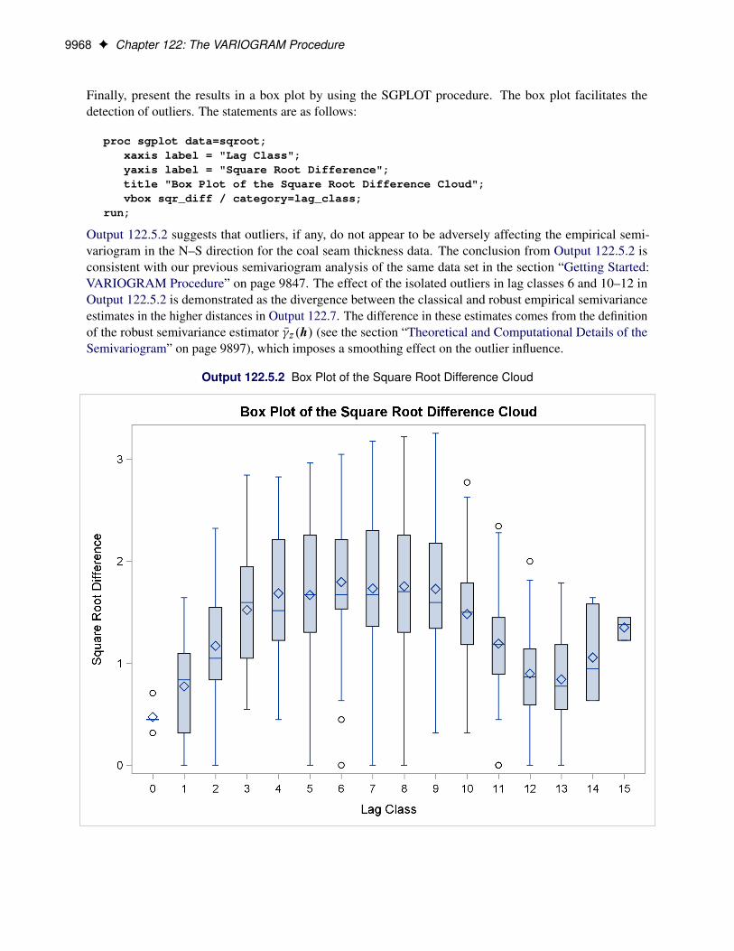
9968 F Chapter 122: The VARIOGRAM Procedure
Finally, present the results in a box plot by using the SGPLOT procedure. The box plot facilitates thedetection of outliers. The statements are as follows:
proc sgplot data=sqroot;xaxis label = "Lag Class";yaxis label = "Square Root Difference";title "Box Plot of the Square Root Difference Cloud";vbox sqr_diff / category=lag_class;
run;
Output 122.5.2 suggests that outliers, if any, do not appear to be adversely affecting the empirical semi-variogram in the N–S direction for the coal seam thickness data. The conclusion from Output 122.5.2 isconsistent with our previous semivariogram analysis of the same data set in the section “Getting Started:VARIOGRAM Procedure” on page 9847. The effect of the isolated outliers in lag classes 6 and 10–12 inOutput 122.5.2 is demonstrated as the divergence between the classical and robust empirical semivarianceestimates in the higher distances in Output 122.7. The difference in these estimates comes from the definitionof the robust semivariance estimator N z.h/ (see the section “Theoretical and Computational Details of theSemivariogram” on page 9897), which imposes a smoothing effect on the outlier influence.
Output 122.5.2 Box Plot of the Square Root Difference Cloud

References F 9969
References
Anselin, L. (1996). “The Moran Scatterplot as an ESDA Tool to Assess Local Instability in SpatialAssociation.” In Spatial Analytical Perspectives on GIS, edited by M. Fischer, H. Scholten, and D. Unwin,111–125. London: Taylor & Francis.
Banerjee, S., Carlin, B. P., and Gelfand, A. E. (2004). Hierarchical Modeling and Analysis for Spatial Data.Boca Raton, FL: Chapman & Hall/CRC.
Chilès, J. P., and Delfiner, P. (1999). Geostatistics: Modeling Spatial Uncertainty. New York: John Wiley &Sons.
Christakos, G. (1992). Random Field Models in Earth Sciences. New York: Academic Press.
Cliff, A. D., and Ord, J. K. (1981). Spatial Processes: Models and Applications. London: Pion Ltd.
Cressie, N. (1985). “Fitting Variogram Models by Weighted Least Squares.” Mathematical Geology17:563–570.
Cressie, N. (1993). Statistics for Spatial Data. Rev. ed. New York: John Wiley & Sons.
Cressie, N., and Hawkins, D. M. (1980). “Robust Estimation of the Variogram: I.” Mathematical Geology12:115–125.
Deutsch, C. V., and Journel, A. G. (1992). GSLIB: Geostatistical Software Library and User’s Guide. NewYork: Oxford University Press.
Geary, R. C. (1954). “The Contiguity Ratio and Statistical Mapping.” Incorporated Statistician 5:115–145.
Goovaerts, P. (1997). Geostatistics for Natural Resources Evaluation. New York: Oxford University Press.
Hohn, M. E. (1988). Geostatistics and Petroleum Geology. New York: Van Nostrand Reinhold.
Jian, X., Olea, R. A., and Yu, Y.-S. (1996). “Semivariogram Modeling by Weighted Least Squares.”Computers and Geosciences 22:387–397.
Journel, A. G., and Huijbregts, C. J. (1978). Mining Geostatistics. New York: Academic Press.
Matheron, G. (1963). “Principles of Geostatistics.” Economic Geology 58:1246–1266.
Moran, P. A. P. (1950). “Notes on Continuous Stochastic Phenomena.” Biometrika 37:17–23.
Olea, R. A. (1999). Geostatistics for Engineers and Earth Scientists. Boston: Kluwer Academic.
Olea, R. A. (2006). “A Six-Step Practical Approach to Semivariogram Modeling.” Stochastic EnvironmentalResearch and Risk Assessment 20:307–318.
Schabenberger, O., and Gotway, C. A. (2005). Statistical Methods for Spatial Data Analysis. Boca Raton,FL: Chapman & Hall/CRC.
Stein, M. L. (1988). “Asymptotically Efficient Prediction of a Random Field with a Misspecified CovarianceFunction.” Annals of Statistics 16:55–63.

Subject Index
AIC, see fit criteria (VARIOGRAM)Akaike information criterion, see fit criteria
(VARIOGRAM)angle
classes (VARIOGRAM), 9872, 9873, 9875, 9902,9903
tolerance (VARIOGRAM), 9870, 9873, 9875,9902, 9903
anisotropygeometric (VARIOGRAM), 9900major axis (VARIOGRAM), 9900, 9950minor axis (VARIOGRAM), 9900, 9950VARIOGRAM procedure, 9873, 9900, 9911,
9941zonal (VARIOGRAM), 9900
autocorrelationGeary’s c coefficient (VARIOGRAM), 9846,
9870, 9920Moran scatter plot (VARIOGRAM), 9855, 9862,
9922Moran’s I coefficient (VARIOGRAM), 9846,
9870, 9920VARIOGRAM procedure, 9846, 9919
autocorrelation weightsrow-averaged (VARIOGRAM), 9855, 9920, 9923standardized (VARIOGRAM), 9920VARIOGRAM procedure, 9919
bandwidthVARIOGRAM procedure, 9872, 9875, 9904
boundary constraintsVARIOGRAM procedure, 9889, 9891
class, see angle classes (VARIOGRAM), see fitequivalence classes (VARIOGRAM), see lagclassification (VARIOGRAM)
collocationVARIOGRAM procedure, 9901, 9922
confidence levelVARIOGRAM procedure, 9869, 9877
confidence limitsVARIOGRAM procedure, 9872, 9878
constraintsboundary (VARIOGRAM), 9889, 9891scale (VARIOGRAM), 9890
correlationlength (VARIOGRAM), 9909radius (VARIOGRAM), 9909range (VARIOGRAM), 9909
covarianceVARIOGRAM procedure, 9846, 9899, 9962
covariogramVARIOGRAM procedure, 9962
cubic semivariance modelVARIOGRAM procedure, 9879, 9895
distance, see lag (VARIOGRAM)classification (VARIOGRAM), 9904
equivalence class, see fit equivalence classes(VARIOGRAM)
ergodicityVARIOGRAM procedure, 9900
estimationVARIOGRAM procedure, 9847
exploratory data analysisVARIOGRAM procedure, 9848
exponential semivariance modelVARIOGRAM procedure, 9879, 9895
fit, see also semivariogram theoretical model fitting(VARIOGRAM)
automated (VARIOGRAM), 9911criteria (VARIOGRAM), 9916equivalence classes (VARIOGRAM), 9918quality (VARIOGRAM), 9915
Gaussian semivariance modelVARIOGRAM procedure, 9879, 9895
Geary’s c coefficient, see autocorrelation
initial valuesVARIOGRAM procedure, 9887, 9913
isotropy, see anisotropy (VARIOGRAM)VARIOGRAM procedure, 9849, 9873, 9900
krigingordinary kriging (VARIOGRAM), 9847
lagclassification (VARIOGRAM), 9850, 9903count (VARIOGRAM), 9850, 9905distance (VARIOGRAM), 9849, 9872, 9905,
9908number of point pairs in (VARIOGRAM), 9907pairwise distance (VARIOGRAM), 9849tolerance (VARIOGRAM), 9872, 9904VARIOGRAM procedure, 9849

Matérn, see also semivariogram theoretical models(VARIOGRAM)
Matérnmodel fitting (VARIOGRAM), 9918
Matérn semivariance modelVARIOGRAM procedure, 9879, 9895
mean trend, see surface trend (VARIOGRAM)measures of spatial continuity
VARIOGRAM procedure, 9846, 9897, 9962model fitting, see semivariogram theoretical model
fitting (VARIOGRAM)VARIOGRAM procedure, 9931
modeling, see semivariogram theoretical model fitting(VARIOGRAM)
Moran scatter plot, see autocorrelationMoran’s I coefficient, see autocorrelation
nested modelsVARIOGRAM procedure, 9897
nonrandom trend, see surface trendnormality assumption
VARIOGRAM procedure, 9870, 9921nugget effect
VARIOGRAM procedure, 9883, 9894, 9897
ODS graph namesVARIOGRAM procedure, 9930
ODS GraphicsVARIOGRAM procedure, 9863
ODS table namesVARIOGRAM procedure, 9929
output data setsVARIOGRAM procedure, 9862, 9863, 9907,
9924–9926
pairwise distance, see also lag classification(VARIOGRAM)
distribution (VARIOGRAM), 9905VARIOGRAM procedure, 9850
panels (VARIOGRAM procedure), see plots(VARIOGRAM procedure)
pentaspherical semivariance modelVARIOGRAM procedure, 9879, 9895
plots (VARIOGRAM procedure)Fit, 9930Fit panel, 9930Moran scatter plot, 9930Observations, 9930Pairs, 9930Pairwise distance distribution, 9930panels, 9864, 9948, 9955, 9958Semivariogram, 9930Semivariogram panel, 9930
point pairsVARIOGRAM procedure, 9849, 9898, 9901
power semivariance modelVARIOGRAM procedure, 9879, 9895
predictionVARIOGRAM procedure, 9847
preliminary data analysis, see exploratory data analysispseudo-semivariance
VARIOGRAM procedure, 9899pseudo-semivariogram
VARIOGRAM procedure, 9899, 9955
randomization assumptionVARIOGRAM procedure, 9870, 9921
rangeeffective (VARIOGRAM), 9894practical (VARIOGRAM), 9894VARIOGRAM procedure, 9894
scale constraintsVARIOGRAM procedure, 9890
semivariance, see also semivariogramclassical (VARIOGRAM), 9852, 9898computation (VARIOGRAM), 9909empirical (VARIOGRAM), 9898robust (VARIOGRAM), 9852, 9874, 9898theoretical models, 9895variance (VARIOGRAM), 9898VARIOGRAM procedure, 9846, 9897, 9962
semivariogramanalysis (VARIOGRAM), 9848and covariogram (VARIOGRAM), 9962computation (VARIOGRAM), 9848empirical (VARIOGRAM), 9848, 9898parameters (VARIOGRAM), 9894robust (VARIOGRAM), 9898theoretical model fitting, 9856, 9875, 9887, 9911,
9951theoretical models (VARIOGRAM), 9848, 9849,
9892VARIOGRAM procedure, 9846, 9897
sillVARIOGRAM procedure, 9894
sine hole effect semivariance modelVARIOGRAM procedure, 9879, 9895
spatial continuityVARIOGRAM procedure, 9846, 9847, 9897,
9899, 9955, 9962spatial dependence, see spatial continuityspatial lag, see also autocorrelation Moran scatter plot
(VARIOGRAM)VARIOGRAM procedure, 9922
spatial predictionVARIOGRAM procedure, 9847, 9899
spatial random fieldautocorrelation (VARIOGRAM), 9919
ergodicity (VARIOGRAM), 9900intrinsically stationary (VARIOGRAM), 9899isotropic (VARIOGRAM), 9900, 9911realization (VARIOGRAM), 9892spatial continuity (VARIOGRAM), 9897, 9955VARIOGRAM procedure, 9892
spatial structure, see spatial continuityspherical semivariance model
VARIOGRAM procedure, 9879, 9895square root difference cloud
VARIOGRAM procedure, 9966SRF, see spatial random fieldSSE, see fit criteria (VARIOGRAM)standard errors
VARIOGRAM procedure, 9847stationarity
intrinsic (VARIOGRAM), 9899second-order (VARIOGRAM), 9899, 9964VARIOGRAM procedure, 9893
stochastic analysisVARIOGRAM procedure, 9847
stochastic modeling, see semivariogram theoreticalmodel fitting (VARIOGRAM), see spatialprediction (VARIOGRAM)
stochastic spatial prediction, see spatial prediction(VARIOGRAM)
surface trendVARIOGRAM procedure, 9846, 9849, 9898,
9910, 9941, 9945systematic trend, see surface trend
tables (VARIOGRAM procedure)Approximate Correlation Matrix, 9929Approximate Covariance Matrix, 9929Autocorrelation Statistics, 9855, 9927, 9929Convergence Status, 9929Empirical Semivariogram, 9853, 9927, 9929Fit Summary, 9929Fitting General Information, 9929Iteration History, 9929Lagrange Multipliers, 9929Model Information, 9929Number of Observations, 9927Optimization Information, 9929Optimization Input Options, 9929Optimization Results, 9929Pairs Information, 9850, 9907–9909, 9927, 9929Pairwise Distance Intervals, 9850, 9907–9909,
9927, 9929, 9943, 9950Parameter Estimates, 9929Parameter Estimates Results, 9929Parameter Search, 9929Problem Description, 9929PROC VARIOGRAM statements, 9861
Projected Gradient, 9929Starting Parameter Estimates, 9929
theoretical semivariogram models, see semivariogram(VARIOGRAM)
tolerance, see angle tolerance (VARIOGRAM), see lagtolerance (VARIOGRAM)
trend, see surface trend (VARIOGRAM)
uncertaintyVARIOGRAM procedure, 9847
VARIOGRAM procedureangle classes, 9872, 9873, 9875, 9902, 9903angle tolerance, 9870, 9873, 9875, 9902, 9903anisotropy, 9873, 9941autocorrelation, 9846, 9919autocorrelation weights, 9919bandwidth, 9872, 9875, 9904boundary constraints, 9889, 9891collocation, 9901, 9922confidence level, 9869, 9877confidence limits, 9872, 9878correlation measures, 9909covariance, 9846, 9899, 9962covariance matrix, 9886cubic semivariance model, 9879, 9895cutoff distance, 9874DATA= data set, 9861distance classes, 9905, 9907, 9908distance classification, 9903, 9904distance interval, 9850ergodicity, 9900estimation, 9847examples, 9848, 9931, 9941, 9955, 9962, 9966exploratory data analysis, 9848exponential semivariance model, 9879, 9895Gaussian semivariance model, 9879, 9895Geary’s c coefficient, 9846, 9870, 9920grid search, 9887initial values, 9887, 9913input data set, 9861isotropy, 9873lag, 9849, 9905, 9907lag distance, 9872, 9905lag tolerance, 9872Matérn semivariance model, 9879, 9895measures of spatial continuity, 9846, 9897, 9962model fitting, 9856, 9875, 9887, 9911, 9931, 9951Moran scatter plot, 9855, 9862, 9922Moran’s I coefficient, 9846, 9870, 9920nested models, 9897normality assumption, 9870, 9921nugget effect, 9883, 9894, 9897ODS graph names, 9930
ODS Graphics, 9863ODS table names, 9929ordinary kriging, 9847OUTACWEIGHTS= data set, 9862OUTDIST= data set, 9862, 9907OUTMORAN= data set, 9862OUTPAIR= data set, 9863output data sets, 9862, 9863, 9924–9926OUTVAR= data set, 9863pairwise distance, 9850, 9872panel plots, 9863pentaspherical semivariance model, 9879, 9895point pairs, 9849, 9898, 9901power semivariance model, 9879, 9895prediction, 9847pseudo-semivariance, 9899pseudo-semivariogram, 9899, 9955randomization assumption, 9870, 9921scale constraints, 9890semivariance, 9846, 9897, 9962semivariance computation, 9909semivariance, classical, 9852, 9898semivariance, empirical, 9898semivariance, robust, 9852, 9874, 9898semivariance, variance, 9898semivariogram, 9846, 9897semivariogram analysis, 9848semivariogram and covariogram, 9962semivariogram computation, 9848semivariogram effective range, 9894semivariogram parameters, 9894semivariogram range, 9894semivariogram sill, 9894semivariogram, empirical, 9848, 9898semivariogram, robust, 9898sine hole effect semivariance model, 9879, 9895spatial continuity, 9846, 9847, 9897, 9899, 9955,
9962spatial lag, 9922spatial prediction, 9847, 9899spatial random field, 9892, 9897, 9899, 9900,
9911, 9919, 9955spherical semivariance model, 9879, 9895square root difference cloud, 9966standard errors, 9847stationarity, 9893, 9899, 9964stochastic analysis, 9847surface trend, 9846, 9849, 9898, 9910, 9941, 9945theoretical semivariogram models, 9848, 9849,
9856, 9892, 9895, 9951uncertainty, 9847weighted average, 9855, 9922
VARIOGRAM procedure, plotsFit, 9930
Fit panel, 9930Moran scatter plot, 9930Observations, 9930Pairs, 9930Pairwise distance distribution, 9930Semivariogram, 9930Semivariogram panel, 9930
VARIOGRAM procedure, tablesApproximate Correlation Matrix, 9929Approximate Covariance Matrix, 9929Autocorrelation Statistics, 9855, 9927, 9929Convergence Status, 9929Empirical Semivariogram, 9853, 9927, 9929Fit Summary, 9929Fitting General Information, 9929Iteration History, 9929Lagrange Multipliers, 9929Model Information, 9929Number of Observations, 9927Optimization Information, 9929Optimization Input Options, 9929Optimization Results, 9929Pairs Information, 9850, 9907–9909, 9927, 9929Pairwise Distance Intervals, 9850, 9907–9909,
9927, 9929, 9943, 9950Parameter Estimates, 9929Parameter Estimates Results, 9929Parameter Search, 9929Problem Description, 9929PROC VARIOGRAM statements, 9861Projected Gradient, 9929Starting Parameter Estimates, 9929
weighted averageVARIOGRAM procedure, 9855, 9922
weighted least squares, see fit criteria (VARIOGRAM)WSSE, see fit criteria (VARIOGRAM)

Syntax Index
ALPHA= optionCOMPUTE statement (VARIOGRAM), 9869MODEL statement (VARIOGRAM), 9877
ANGLETOLERANCE= optionCOMPUTE statement (VARIOGRAM), 9870
AUTOCORRELATION optionVARIOGRAM procedure, COMPUTE statement,
9870AUTOCORRELATION STATISTICS= option
VARIOGRAM procedure, COMPUTE statement,9870
BANDWIDTH= optionCOMPUTE statement (VARIOGRAM), 9872
BY statementVARIOGRAM procedure, 9868
CHOOSE= optionMODEL statement (VARIOGRAM), 9877
CL optionCOMPUTE statement (VARIOGRAM), 9872MODEL statement (VARIOGRAM), 9878
COMPUTE statementVARIOGRAM procedure, 9869
COORDINATES statementVARIOGRAM procedure, 9874
CORRB optionMODEL statement (VARIOGRAM), 9886
COVB optionMODEL statement (VARIOGRAM), 9886
DATA= optionPROC VARIOGRAM statement, 9861
DEPSILON= optionCOMPUTE statement (VARIOGRAM), 9872
DETAILS optionMODEL statement (VARIOGRAM), 9886
DIRECTIONS statementVARIOGRAM procedure, 9875
EQCONS= optionPARMS statement (VARIOGRAM), 9889
EQUIVTOL= optionMODEL statement (VARIOGRAM), 9878
FIT optionMODEL statement (VARIOGRAM), 9878
FORM= optionMODEL statement (VARIOGRAM), 9878
GRADIENT optionMODEL statement (VARIOGRAM), 9887
HOLD= optionPARMS statement (VARIOGRAM), 9889
ID statementVARIOGRAM procedure, 9875
IDGLOBAL optionPROC VARIOGRAM statement, 9862
IDNUM optionPROC VARIOGRAM statement, 9862
LABEL= optionSTORE statement (VARIOGRAM), 9892
LAGDISTANCE= optionCOMPUTE statement (VARIOGRAM), 9872
LAGTOLERANCE= optionCOMPUTE statement (VARIOGRAM), 9873
LOWERB= optionPARMS statement (VARIOGRAM), 9889
MAXLAGS= optionCOMPUTE statement (VARIOGRAM), 9873
MAXSCALE= optionPARMS statement (VARIOGRAM), 9890
MDATA= optionMODEL statement (VARIOGRAM), 9881
MODEL statementVARIOGRAM procedure, 9875
MTOGTOL= optionMODEL statement (VARIOGRAM), 9887
NDIRECTIONS= optionCOMPUTE statement (VARIOGRAM), 9873
NEPSILON= optionMODEL statement (VARIOGRAM), 9883
NHCLASSES= optionCOMPUTE statement (VARIOGRAM), 9874
NLOPTIONS statementVARIOGRAM procedure, 9891
NOBOUND optionPARMS statement (VARIOGRAM), 9890
NOFIT optionMODEL statement (VARIOGRAM), 9887
NOITPRINT optionMODEL statement (VARIOGRAM), 9887
NOPRINT optionPROC VARIOGRAM statement, 9862

NOVARIOGRAM optionCOMPUTE statement (VARIOGRAM), 9874
NUGGET= optionMODEL statement (VARIOGRAM), 9883
OUTACWEIGHTS= optionPROC VARIOGRAM statement, 9862
OUTDISTANCE= optionPROC VARIOGRAM statement, 9862
OUTMORAN= optionPROC VARIOGRAM statement, 9862
OUTPAIR= optionPROC VARIOGRAM statement, 9863
OUTPDISTANCE= optionCOMPUTE statement (VARIOGRAM), 9874
output data setsVARIOGRAM procedure, 9846
OUTVAR= optionPROC VARIOGRAM statement, 9863
PARMS statementVARIOGRAM procedure, 9887
PARMSDATA= optionPARMS statement (VARIOGRAM), 9890
PDATA= optionPARMS statement (VARIOGRAM), 9890
PLOTS optionVARIOGRAM procedure, PROC VARIOGRAM
statement, 9863PLOTS(ONLY) option
VARIOGRAM procedure, PROC VARIOGRAMstatement, 9864
PLOTS(UNPACKPANEL) optionVARIOGRAM procedure, PROC VARIOGRAM
statement, 9864PLOTS=ALL option
VARIOGRAM procedure, PROC VARIOGRAMstatement, 9864
PLOTS=EQUATE optionVARIOGRAM procedure, PROC VARIOGRAM
statement, 9864PLOTS=FITPLOT option
VARIOGRAM procedure, PROC VARIOGRAMstatement, 9864
PLOTS=MORAN optionVARIOGRAM procedure, PROC VARIOGRAM
statement, 9865PLOTS=NONE option
VARIOGRAM procedure, PROC VARIOGRAMstatement, 9866
PLOTS=OBSERVATIONS optionVARIOGRAM procedure, PROC VARIOGRAM
statement, 9866PLOTS=PAIRS option
VARIOGRAM procedure, PROC VARIOGRAMstatement, 9867
PLOTS=SEMIVARIOGRAM optionVARIOGRAM procedure, PROC VARIOGRAM
statement, 9868PROC VARIOGRAM statement, see VARIOGRAM
procedure
RANGE= optionMODEL statement (VARIOGRAM), 9883
RANGELAG= optionMODEL statement (VARIOGRAM), 9884
RANKEPS= optionMODEL statement (VARIOGRAM), 9884
ROBUST optionCOMPUTE statement (VARIOGRAM), 9874
SCALE= optionMODEL statement (VARIOGRAM), 9885
SMOOTH= optionMODEL statement (VARIOGRAM), 9885
STORE statementVARIOGRAM procedure, 9891
UPPERB= optionPARMS statement (VARIOGRAM), 9891
VAR statementVARIOGRAM procedure, 9892
VARIOGRAM procedure, 9846output data sets, 9846syntax, 9861
VARIOGRAM procedure, BY statement, 9868VARIOGRAM procedure, COMPUTE statement, 9869
ALPHA= option, 9869ANGLETOLERANCE= option, 9870AUTOCORRELATION option, 9870AUTOCORRELATION STATISTICS= option,
9870BANDWIDTH= option, 9872CL option, 9872DEPSILON= option, 9872LAGDISTANCE= option, 9872LAGTOLERANCE= option, 9873MAXLAGS= option, 9873NDIRECTIONS= option, 9873NHCLASSES= option, 9874NOVARIOGRAM option, 9874OUTPDISTANCE= option, 9874ROBUST option, 9874
VARIOGRAM procedure, COORDINATES statement,9874
XCOORD= option, 9874YCOORD= option, 9874
VARIOGRAM procedure, DIRECTIONS statement,9875
VARIOGRAM procedure, ID statement, 9875VARIOGRAM procedure, MODEL statement, 9875
ALPHA= option, 9877CHOOSE= option, 9877CL option, 9878CORRB option, 9886COVB option, 9886DETAILS option, 9886EQUIVTOL= option, 9878FIT option, 9878FORM= option, 9878GRADIENT option, 9887MDATA= option, 9881MTOGTOL= option, 9887NEPSILON= option, 9883NOFIT option, 9887NOITPRINT option, 9887NUGGET= option, 9883RANGE= option, 9883RANGELAG= option, 9884RANKEPS= option, 9884SCALE= option, 9885SMOOTH= option, 9885
VARIOGRAM procedure, NLOPTIONS statement,9891
VARIOGRAM procedure, PARMS statement, 9887EQCONS= option, 9889HOLD= option, 9889LOWERB= option, 9889MAXSCALE= option, 9890NOBOUND option, 9890PARMSDATA= option, 9890PDATA= option, 9890UPPERB= option, 9891
VARIOGRAM procedure, PROC VARIOGRAMstatement, 9861
DATA= option, 9861IDGLOBAL option, 9862IDNUM option, 9862NOPRINT option, 9862OUTACWEIGHTS= option, 9862OUTDISTANCE= option, 9862OUTMORAN= option, 9862OUTPAIR= option, 9863OUTVAR= option, 9863PLOTS option, 9863PLOTS(ONLY) option, 9864PLOTS(UNPACKPANEL) option, 9864PLOTS=ALL option, 9864PLOTS=EQUATE option, 9864PLOTS=FITPLOT option, 9864PLOTS=MORAN options, 9865
PLOTS=NONE option, 9866PLOTS=OBSERVATIONS option, 9866PLOTS=PAIRS option, 9867PLOTS=SEMIVARIOGRAM option, 9868
VARIOGRAM procedure, STORE statement, 9891LABEL= options, 9892
VARIOGRAM procedure, VAR statement, 9892
XCOORD=optionCOORDINATES statement (VARIOGRAM),
9874
YCOORD=optionCOORDINATES statement (VARIOGRAM),
9874