
SAS_Manual.pdf
163
Jordan University of Science and Technology USER’S MANUAL FOR SAS-MCT 4.0 A Computer Program for Stability Analysis of Slopes Using Monte Carlo Technique By Abdallah I. Husein Malkawi, Ph.D. Professor and Dean of Research Geotechnical and Dam Engineering Email: [email protected] Waleed Falih Hassan, M.Sc. Research Associate Geotechnical Engineering Research Group Civil Engineering Department Jordan University of Science and Technology Irbid 22110 – JORDAN Version 4.0 May, 2003
-
Upload
eduardo-infante -
Category
Documents
-
view
223 -
download
1
Transcript of SAS_Manual.pdf
Jordan University of Science and Technology
USER’S MANUAL
FOR
SAS-MCT 4.0
A Computer Program for Stability Analysis of Slopes Using Monte Carlo Technique
By
Abdallah I. Husein Malkawi, Ph.D.
Professor and Dean of Research Geotechnical and Dam Engineering
Email: [email protected]
Waleed Falih Hassan, M.Sc.
Research Associate
Geotechnical Engineering Research Group
Civil Engineering Department Jordan University of Science and Technology
Irbid 22110 – JORDAN
Version 4.0 May, 2003

ii
Copyright © Geotechnical Engineering Research Group 2003 This research was partly conducted at Jordan University of Science and Technology and partly supported by Deanship of Research. The authorship rights are reserved for Jordan University of Science and Technology and the authors.
iii
PREFACE Development of SAS-MCT began in 1997 at Jordan University of Science and Technology as an initiative to develop an easy-to-use computer program for solving complicated slope stability problems involving earth structures such as natural slopes, excavations, dams, or man-made embankments. A new automatic search procedure coupled with a new Monte-Carlo method of both random jumping and random walking types for locating the global critical circular and non-circular slip surface was developed and integrated in the code. This procedure was published in the following well known international Journals;
Husein Malkawi, A.I.; Hassan, W.F and Abdulla, F. (2000) “Uncertainty and reliability analysis applied to slope stability” Structural Safety Journal, 22, 161-187. Husein Malkawi, A.I.; Hassan, W.F. and S.K. Sarma (2001) "A global search method for locating general slip surface using Monte Carlo Techniques", ASCE Geotechnical and Geoenvironmental Journal, August. Husein Malkawi, A.I.; Hassan, W.F. and S.K. Sarma (2001) "An efficient search method for locating circular slip surface using Monte Carlo Technique", Canadian Geotechnical Journal., October. Husein Malkawi, A.I.; Hassan, W.F. and S.K. Sarma (2002) "Closure to discussion of - a global search method for locating general slip surface using Monte Carlo Techniques", by Gautam Bhattacharya, ASCE Geotechnical and Geoenvironmental Journal, December.
Husein Malkawi, A.I.; Hassan, W.F. and S.K. Sarma (2003) "Reply to discussion of - an efficient search method for locating circular slip surface using Monte Carlo Technique", By V.R. Greco, Canadian Geotechnical Journal., February.
The first and second versions of SAS-MCT Software were released in 1999; these versions run under DOS operating systems. Two years later i.e., in 2001, the third version was released SAS-MCT 3.0. The main code was kept in Fortran language whereas the graphics user interface was coded by Dr. Nezar A. Hammouri in Visual Basic. This version runs on PC’s using Windows operating system. Later on, the main code and the supporting graphics were converted into Microsoft® Visual Basic 6.0 by Eng. Mohammad Yamin. This new version SAS-MCT 4.0 runs on PC’s Windows operating systems. Today, there are two versions of the software: SAS-MCT4.0 Standard for ordinary users and SAS-MCT4.0 PRO for researchers and professionals. The SAS-MCT4.0 PRO is more accurate and usually requires more computational time, especially when rigorous methods are used.
iv
TABLE OF CONTENTS
CHAPTER I INTRODUCTION 1
CHAPTER II DREVATION OF FACTOR OF SAFFTY 3
Introduction 3 Stability Methods used by SAS-MCT Program 7 Ordinary or Fellenius Method 8
Simplified Bishop Method 10 Janbu’s Simplified Method 11 Morgenstern- Price Method 13 Spencer’s Method 16 Three-Dimension Stability Analysis 17 General 17 Bishop method in Three-Dimensions 18 Janbu’s Method in Three-Dimensions 21
CHAPTER III MONTE-CARLO TECHNIAUE TO ESTIMETE UNCERTAINTY 22 Introduction 22
Uncertainty in Soil Properties 22 Safety Factor Distribution 24 Normal Distribution Generation 25 Log-Normal Distribution Generation 27 First-Order Second-Moment Approximation 29
CHAPTER IV SAS-MCT PROGRAM 31
Program Features 31 Program Description and Organization 38
CHAPTER V ILLUSTRATIVE EXAMPLES 40
EXAMPLE 1 40 EXAMPLE 2 70 EXAMPLE 3 95 EXAMPLE 4 104 EXAMPLE 5 134

1
CHAPTER I
Introduction Preamble Stability Analysis Slopes using Monte – Carlo Technique (SAS – MCT)
Version 4.0 is a computer software designed to operate on Windows
operating system. The program is capable of analyzing the stability of man –
made or natural slopes under static and earthquake loading. The program
uses a new developed automatic search procedure coupled with a new
Monte-Carlo method of both random jumping and random walking types for
locating the global critical circular and non-circular slip surface. Calculation of
the factor of safety against instability is performed by one of the following
limiting equilibrium based methods. Ordinary method, Bishop’s simplified
method, Janbu’s method, Spencer’s method, and the generalized limited
equilibrium (GLE) method, a discrete version of Morgenstern – Price method.
The program provides a number of high quality plots. These plots can be
viewed and easily sent to printers. Water can be defined in terms of pore
water pressure ratio (ru) or as a phreatic surface. Total and effective stress
analysis can be performed. Specific circular and non circular slip surface can
be defined and analyzed. Analysis is performed using SI units (kN, m) or
British Units (lbf, ft). Point loads and surcharge loads can be included in the
analysis; inclination of these loads is specified with respect to the vertical axis.
Detailed output files are created to provide the user with extensive information
about the output. In details, the program features the following:
1- Two-Dimensional analysis of slopes assuming circular slip
surface and using either one of the following methods as
specified by the user: Ordinary method, Bishop’s method,
Janbu’s method, Spencer’s method, and the generalized Limited
Equilibrium (GLE) method, which is a discrete version of
Morgenstern-Price method.

2
2- The program can be used to search for critical slip surfaces
based on maximum probability of failure. First order second
moment approximation is used to estimate the reliability index
(β). This option is valid only for Ordinary method of slices.
3- A two-dimensional analysis of slope stability assuming irregular slip
surfaces and using one of the following methods: Janbu’s method,
Spencer’s method, and Morgenstern-Price method (GLE). In this
respect, the program searches for the most critical slip surface by
representing every trial surface by 4,5,6,… to 12 vertices trying to
simulate the shape of the real slip surface. The most critical slip
surface corresponding to these vertices will be also shown graphically.
4- A seismic slope stability analysis using the peseudo-static approach.
The program computes the reduction in the factor of safety due to the
specified acceleration input expressed in percent of ground
acceleration (g).
5- Three-dimensional slope stability analysis using one of the extensions
of Bishop’s or Janbu’s two-dimensional methods.
6- Reliability Analysis is performed using Monte-Carlo simulation
technique. Normal and log normal distribution are considered. The
program generates a large number of different expected soil
parameters and calculates the safety factor for each random set.
These trials are used to construct the distribution of the safety factor.
The corresponding reliability index (β) and the probability of failure Pf
can be obtained. Soil parameters can be assumed to follow either
normal or log-normal distribution.

3
CHAPTER II
Derivation for Factor of Safety
Introduction
The main goal of slope stability analysis is to determine the most
critical failure surface and its associated minimum factor of safety. The factor
of safety is defined as a ratio of resisting force to driving force, both applied
along the failure surface.
The shape of the failure surface may be quite irregular, depending on
the homogeneity of the materials of the slope. If the material is homogeneous,
the most probable critical failure surface will be cylindrical, because a circle
has the least surface area per unit mass; the surface area is being related to
the resisting force and the mass to the driving force. Practically, all stability
analyses of slopes are based on the concept of limiting equilibrium. In most
methods of limiting equilibrium, only the concept of statics is applied. Except
in the simplest cases, most problems in slope stability are statically
indeterminate. As a result, some simplifying assumptions are made in order to
determine a unique factor of safety. Due to the differences in assumptions
variety of methods, which result in different values for the calculated factor of
safety, have been developed. The most popular methods are Fellenius
(1936), Bishop (1955), Janbu (1954, 1973), Morgenstern and Price (1965),
Spencer (1967), and Sarma (1973,1979). Some of these methods satisfy only
overall moment equilibrium, like Fellenius and simplified Bishop methods that
are both applicable only to circular failure surfaces. On the other hand, Janbu,
Morgenstern-price, Spencer, and Sarma methods satisfy both moment and
force equilibrium and are applicable to failure surfaces of any shape. All these
methods use the same principle in the analysis of the slope stability, i.e.,
dividing the failure surface into a number of slices.
4
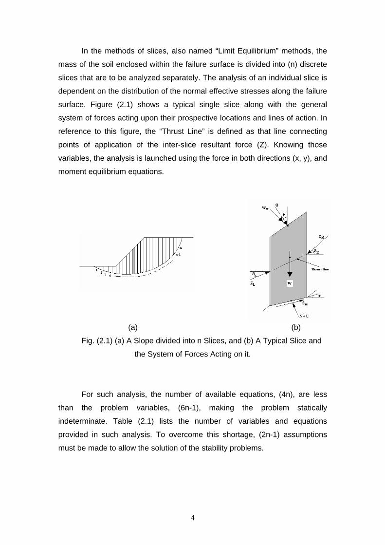
In the methods of slices, also named “Limit Equilibrium” methods, the
mass of the soil enclosed within the failure surface is divided into (n) discrete
slices that are to be analyzed separately. The analysis of an individual slice is
dependent on the distribution of the normal effective stresses along the failure
surface. Figure (2.1) shows a typical single slice along with the general
system of forces acting upon their prospective locations and lines of action. In
reference to this figure, the “Thrust Line” is defined as that line connecting
points of application of the inter-slice resultant force (Z). Knowing those
variables, the analysis is launched using the force in both directions (x, y), and
moment equilibrium equations.
(a) (b)
Fig. (2.1) (a) A Slope divided into n Slices, and (b) A Typical Slice and
the System of Forces Acting on it.
For such analysis, the number of available equations, (4n), are less
than the problem variables, (6n-1), making the problem statically
indeterminate. Table (2.1) lists the number of variables and equations
provided in such analysis. To overcome this shortage, (2n-1) assumptions
must be made to allow the solution of the stability problems.

5
Table 2.1: Equations and Unknowns Encountered in the Method of Slices.
Equations Condition n Moment equilibrium of individual slice. 2n Single slice force equilibrium in two direction.
n Mohr-Coulomb relationship between shear strength and normal effective stress.
4n Total no. of equations. Unknowns Variable
1 Factor of Safety n Normal force at the base of each slice, N’ n Location of normal force. n Mobilized shear force at the base of each slice, Sm.
n-1 Inter-slice resultant force, Z. n-1 Inclination of inter-slice force. n-1 Location of the inter-slice force (line of thrust). 1 Lambda (λ), where λ is a constant value.
6n-1 Total no. of unknowns
The most common assumption made by almost all-slicing methods is
that the slice normal force is located at the slice base mid-length, reducing the
number of variables to (5n-1) and leaving an additional (n-1) assumptions to
be made.
These assumptions are solely related to the inter-slice resultant forces,
where different assumptions result in different analytic methods. These
include Ordinary Method of Slices (OMS) (Fellenius, 1927,1936), Bishop’s
Simplified and Rigorous methods (1955,1955), Janbu’s Simplified and
generalized methods (1954,1957,1973), Lowe and Karafiath’s (1960), Corps
of Engineer’s (1982), Spencer’s (1967,1973), Morgenstern-Price (1965), and
Sarma’s (1973,1979) methods. Some of these methods discard the existence
of inter-slice forces, try to relate their location to ground and slice base
inclinations, assume constant angle of inclinations, or even define a “portion”
of a function describing the points of action of those inter-slice resultant
forces. Table (2.2) summarizes the static equilibrium conditions of the Limit
Equilibrium based methods, where only Bishop’s Rigorous, Spencer’s,
Morgenstern-Price, and Sarma’s methods are found to fully satisfy all
equilibrium conditions.

6
Table (2.2): Comparison between Different Limit Equilibrium Based Methods.
Force equilibrium Method 1st
Direction*2nd
Direction*
Moment equilibrium
Ordinary or Fellenius. Yes No Yes Bishop’s Simplified. Yes No Yes Janbu’s Simplified. Yes Yes No Corps of Engineers. Yes Yes No Lowe and Karafiath. Yes Yes No Janbu’s Generalized. Yes Yes No Bishop Rigorous. Yes Yes Yes Spencer’s. Yes Yes Yes Sarma’s Yes Yes Yes Morgenstern-Price.(GLE) Yes Yes Yes
* Any of the two orthogonal directions can be selected for the summation of forces.
In the next section, a brief description of the most frequently used
methods in slope stability analysis is presented. The program SAS-MCT
incorporated these methods.

7
STABILITY METHODS USED BY SAS-MCT 4.0 PROGRAM:
In order to calculate the factor of safety against sliding for a slope, it is
important that the geotechnical engineer is familiar with the formulation used
by limit equilibrium methods. The complexity of these procedures ranges from
the simple ordinary method, which is suitable for hand calculations, to the
rigorous methods such as Morgenstern-Price method, which really require the
use of a computer. The complete equations for several popular limit
equilibrium methods, which are used in SAS-MCT program, are presented
next. Figure (2.2) depicts the forces acting on a typical slice.
F = factor of safety. ZL = left inter-slice force. ZR = right inter-slice force. δL = left inter-slice force inclination angle.
Sm = mobilized shear strength.
FNbcSm
φtan. ′+′=
δR = right inter-slice force inclination angle.
U = pore water pressure. hL = height of force ZL. W = weight of slice. hR = height of force ZR. Ww = surface water force. α = Inclination of slice base. Q = external surcharge. β = Inclination of slice top. N’ = effective normal force b = width of the slice. Kh = horizontal seismic coefficient. h = average height of the slice. µ = Angle of inclination of external load.
ha = height to the center of the slice.
Fig. (2.2) Forces Acting on a Typical Slice.
8
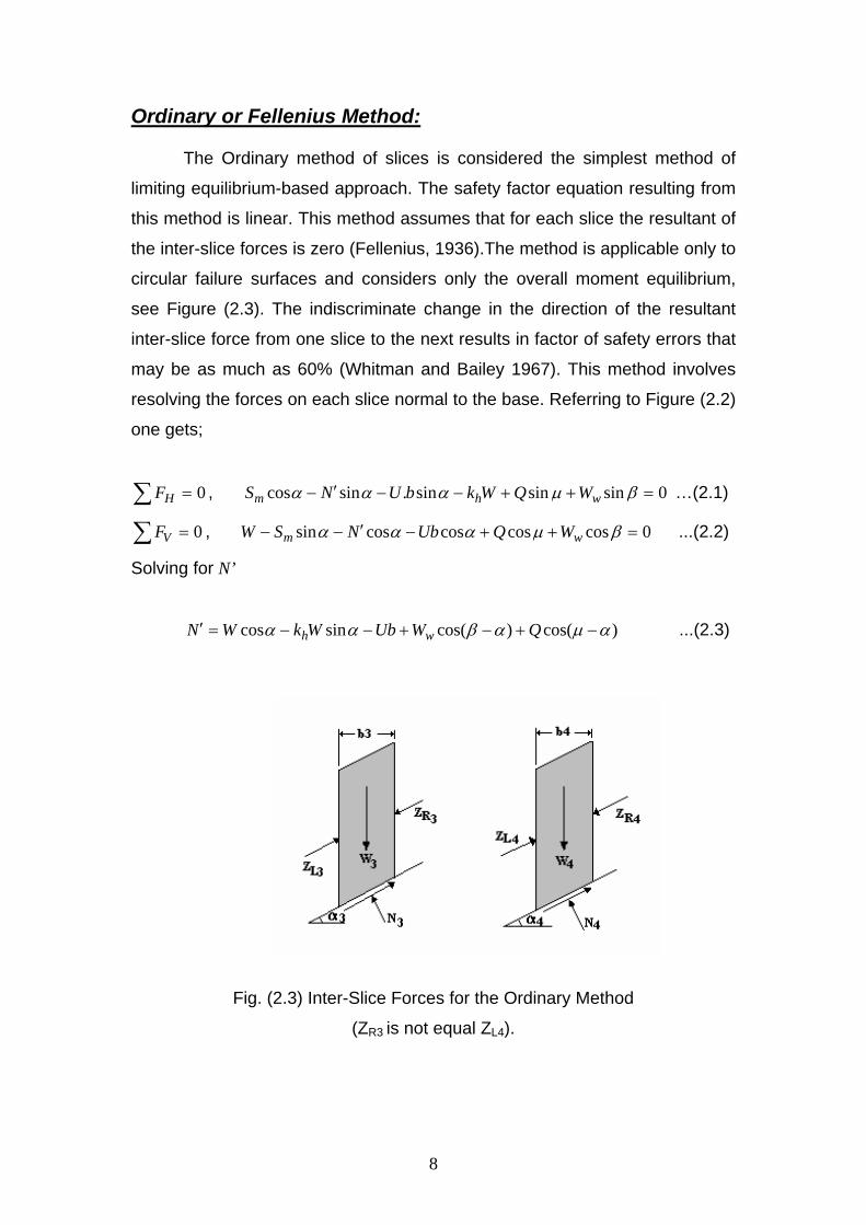
Ordinary or Fellenius Method:
The Ordinary method of slices is considered the simplest method of
limiting equilibrium-based approach. The safety factor equation resulting from
this method is linear. This method assumes that for each slice the resultant of
the inter-slice forces is zero (Fellenius, 1936).The method is applicable only to
circular failure surfaces and considers only the overall moment equilibrium,
see Figure (2.3). The indiscriminate change in the direction of the resultant
inter-slice force from one slice to the next results in factor of safety errors that
may be as much as 60% (Whitman and Bailey 1967). This method involves
resolving the forces on each slice normal to the base. Referring to Figure (2.2)
one gets;
0=∑ HF , 0sinsinsin.sincos =++−−′− βµααα whm WQWkbUNS …(2.1)
0=∑ VF , 0coscoscoscossin =++−′−− βµααα wm WQUbNSW ...(2.2)
Solving for N’
)cos()cos(sincos αµαβαα −+−+−−=′ QWUbWkWN wh ...(2.3)
Fig. (2.3) Inter-Slice Forces for the Ordinary Method
(ZR3 is not equal ZL4).

9
The Mohr-Coulomb mobilized shear strength, Sm , along the base of each
slice is given by;
FNbcSm
φ′′+′=
tan. ...(2.4)
c’ and φtanN ′ are the cohesive and frictional shear strength components of
the soil.
The factor of safety is derived from the summation of moment about
the center of rotation;
Mo =∑ 0
∑=
++=n
iw RQWW
1sin)coscos( αµβ
∑=
−+−n
iW hRQW
1)cos)(sinsin( αµβ
∑∑==
−+−n
iah
n
im hRWKRS
11)cos( α ...(2.5)
Where
R = the radius of the circular failure surface.
h = average height of the slice.
ha = vertical height between center of the base slice and the center of
the slice.
If the factor of safety is assumed to be the same for each slice, then
[ ]
∑ ∑ ∑
∑
= = =
=
−+−+−++
′−+−+−++′= n
i
n
i
n
i
ahWw
h
n
iw
Rh
WkRhQWQWW
bUWkWQWbcF
1 1 1
1
)(cos))(cossinsin(sin)coscos(
tan].sin)cos()cos(cos[sec.
ααµβαµβ
φααβαµαα
…(2.6)

10
Simplified Bishop Method:
In simplified Bishop Method, the inter-slice shear forces are neglected, and only the normal forces are used to define the inter-slice forces, Bishop (1955). This assumption implies that there is no friction between any two slices. In this method, overall moment equilibrium and vertical force equilibrium are satisfied. However, for individual slices, neither moment nor horizontal force equilibrium is satisfied. Although equilibrium conditions are not completely satisfied, the method is, nevertheless, a satisfactory procedure and is recommended for most routine work where the failure surface can be approximated by a circle.
The effective normal forces are derived from the summation of forces
in the vertical direction; refer to Figure (2.2),
∑ = 0VF
⎥⎦⎤
⎢⎣⎡ ++−
′−=′ µβα
αcoscostan1 QWub
FbcW
mN W …(2.7)
where: F
m φααα′
+=tansincos …(2.8)
The factor of safety is derived from the summation of moments about a
common point. Summing the overall moment equilibrium of the forces acting
on each slice about the point of rotation,
∑ =oM
∑ ∑= =
−+−++n
i
n
iWW hRQWRQWW
1 1)cos)(sinsin(sin)coscos( αµβαµβ
0)]cos([11
=−+− ∑∑==
n
iah
n
im hRWkRS α ...(2.9)
Substituting the Mohr-Coulomb failure criterion and solving for the factor of
safety gives;
∑ ∑∑
∑
= ==
=
−+−+−++
′′+′
= n
i
n
i
ahWW
n
i
n
i
RhWk
RhQWQWW
NbcF
1 11
1
)(cos))(cossinsin(sin)coscos(
)0tansec(
ααµβαµβ
φα
…(2.10)

11
Janbu’s Simplified Method: Janbu (1954, 1973) suggested the following method. It satisfies vertical
force equilibrium for each slice and the overall horizontal force equilibrium for
the entire slices mass. It is applicable to failure surfaces of any shape. The
normal force is derived from the summation of vertical forces, with the inter-
slice shear forces ignored. Referring to Figure (2.2) one gets;
∑ = 0VF
µβαα coscossincos)( QWWSubN Wm −−−++′= … (2.11)
αµβαα
coscoscossincos QWWSubN Wm +++−−
=′ …(2.12)
Substituting the value of Sm ,
αµβαα
mQWubF
bcWN W⎭⎬⎫
⎩⎨⎧ ++−
′−=′ coscoscossin ….(2.13)
where F
m φααα′
+=tansincos ….(2.14)
The horizontal force equilibrium equation is used to derive the factor of
safety.
∑ = 0HF
αµβα cossinsinsin)( mWh SQWWkubN +++−+′−= ….(2.15)
Substituting the value of Sm and rearranging the equation for overall
horizontal force equilibrium for the sliding mass,
[ ]∑ ∑ ∑= = =
⎥⎦⎤
⎢⎣⎡ ′′+′
+++−+′−=n
i
n
i
n
iWhH F
NbcQWWkubNF1 1 1
costansinsinsin)( αφµβα …(2.16)
If the factor of safety is assumed to be the same for each slice, then

12
∑∑
∑
==
=
′+−−+
′′+′
= n
iWh
n
i
n
i
NQWWkub
NbcF
11
1
sin)sinsinsin(
cos)tansec(
αµβα
αφα ….(2.17)
On the basis of a strictly limited number of such calculations, Janbu
proposed an empirical correction to be applied to the results of calculations
made using his routine method. This is shown in Figure (2.4). The correction
factor is in the nature of an increase in the factor of safety and depends on the
relative depth of the landslide in relation to its length, and on the nature of the
soil properties (cohesion and angle of internal friction). It has a maximum
value of 13% increase in F. The correction should be applied after the routine
procedure has been followed, i.e. the correction is made to the converged
factor of safety, not during the iterative procedure, as follows:
FfF ocorrected .= ….(2.18)
Where fo is taken from the chart in Figure (2.4).
Fig. (2.4) Janbu’s Correction Factor Chart.

13
MORGENSTERN-PRICE METHOD: Morgenstern-Price (1965) introduced a method in which the inter-slice
resultant force angle is assumed to vary according to an arbitrary function,
f(x). However, the general limit equilibrium (GLE) proposed by (Chugh, 1986,
Fredlund, et al. 1981) is adopted, which is a discrete version of Morgenstern –
Price method. It comprises most of the assumptions used in all methods of
slices. This method follows Spencer’s procedure once the assumed function f
(x) is set to a constant value or to any other shape for a discrete version of a
Morgenstern-Price method. Figure (2.5) illustrates some of the functions used
to describe the variation of inter-slice force angle along the slope.
Fig. (2.5) Function Used to Describe the Variation of Inter-Slice Force Angle.

14
Force Equilibrium
The summing of forces along and normal to the base of the slice are as
follows;
)cos()cos(sin αδαδα −−−+= LLRRm ZZWS
)sin()sin(cos αµαβα −−−−+ QWWk Wh ….(2.19)
)sin()sin(cos αδαδα −−−+=′ LLRR ZZWN
)cos()cos(secsin αµαβαα −+−+−− QWubWk Wh ….(2.20)
From Mohr-Coulomb theory
FNbcSm
φα ′′+′=
tansec. ….(2.21)
Substituting Eq. (2.19) into Eq. (2.21); and eliminating N from Eqs.
(2.20) and (2.21) and solving for ZR;
)cos(tan)sin(tancossec.sin
)cos(tan)sin()cos(tan)sin(
αδφαδφααα
αδφαδαδφαδ
−−′−′−′−
+−−′−−−′−
=RR
LRR
LLR F
WbcFWZFFZ
)cos(tan)sin(]tan)cos()sin([
)cos(tan)sin(cos)tantan(tansec
αδφαδφαβαβ
αδφαδααφφα
−−′−′−+−
−−−′−
′++′+
RR
W
RR
hF
FWF
FWkub
)cos(tan)sin(]tan)cos()sin([
αδφαδφµαµα
−−′−′−+−
−RR F
FQ ….(2.22)

15
Moment Equilibrium
Summing moments of forces about the midpoint at the base of a slice
to determine the location of the inter-slice forces, hR; is on the right-hand side
of each slice,
∑ = 0cM
µβδδαδ sinsin2
sinsin2
)tan2
(cos hQhWbZbZbhZ WRRLLLLL ++++−
0)tan2
(cos =+−− αδ bhZhaWk RRRh ….(2.23)
Solving Eq. (2.23) for hR;
αδδδα
δδ
δδ tan
2tan
22cossintan
2coscos
coscos
2bbb
ZZb
ZZh
ZZh
R
L
R
L
R
L
R
LL
R
L
R
LR −++−=
RR
ah
RRRR
WZ
hWkZhQ
ZhW
δδµ
δβ
coscossin
cossin
−++ ….(2.24)
ZL and hL define the boundary conditions for the first slice and ZR and
hR for the last slice. In many cases, these values are zero.
Equations (2.23) and (2.24) provide two equations for solving the unknown
functions ZR,hR, and δ. In order to complete the system of equations, it is
assumed that;
)(.tan xfλδ = In which f(x) is a function of x and λ is a constant. The problem is now
fully specified, λ and F can be determined by solving equations (2.23) and
(2.24) that satisfy the appropriate boundary conditions. The function f(x) can
be assumed to be one of the functions shown in Figure (2.5).

16
Spencer’s method: Spencer’s method (1967,1973) assumes that the angle of inclination of
the inter-slice forces is constant for all slices. It is a special case of the
Morgenstern-Price method. According to Spencer’s assumption;
)( slicesallforLR δδδ ==
The force equilibrium equation becomes;
)cos(tan)sin(cos)tantan(tansec
)cos(tan)sin(tancossec.sin
αδφαδααφφα
αδφαδφααα
−−′−′−+′
+−−′−
′−′−+=
FFWkub
FWbcFWZZ h
LR
)cos(tan)sin(]tan)cos()sin([
αδφαδφµαµα
−−′−′−−−
+F
FQ)cos(tan)sin(
]tan)cos()sin([αδφαδ
φβαβα−−′−
′−−−+
FFWW ...(2.25)
While the moment equilibrium equation becomes;
αδδα tan2
tan22
tantan2
bbbZZb
ZZh
ZZh
R
L
R
LL
R
LR −++−=
δδ
µδβ
coscossin
cossin
R
ha
RR
WZ
WkhZhQ
ZhW
−++ ...(2.26)
ZL and hL define the boundary conditions for the first slice and ZR and hR
for the last slice. In many cases, these values are zero. By using assumed
values for the solution parameters, F and (δ), and considering the known
boundary conditions, ZL and hL, it becomes possible to use Eqs. (2.25) and
(2.26) in a recursive manner, slice by slice, and evaluate ZR and hR for the last
slice. The calculated values of ZR and hR at the boundary are compared with
the given values. An adjustment is made to the assumed values of F and (δ),
and the procedure is repeated.
The iterations are terminated when the calculated values of ZR and hR
are within an acceptable tolerance to the known values of ZR and hR at the
boundary.
17
Three-Dimension Stability Analysis:
General:
Most of the three-dimensional methods developed are simplified
methods and are not rigorous, since they either neglect the inter-column
forces or make assumptions that have not been completely verified.
Hovland (1977) determined the three-dimensional factor of safety for
several example problems. The solutions indicated that the three-dimensional
analysis of slopes give factors of safety that are smaller than the two-
dimensional factors of safety for a certain method. Hutchinson and Sarma
(1985) pointed out that the ratio F3/F2 can approach 1.0, but should not fall
below 1.0, where F3 and F2 are the 3-D and 2-D factors of safety,
respectively. Hunger (1987), indicated that, for all cases, the ratio F3/F2 was
greater than 1.0. Chen and Chameau (1983) found that the ratio F3/F2 might
be less than 1.0 at certain circumstances. Cavounidis (1987) concluded that
the F3/F2 ratios must be equal to or greater than unity and methods that give
F3/F2 ratios below the unity are not accurate.
In the next section, Bishop and Janbu simplified 2-D methods
extended to 3-D methods and are implemented in the program SAS-MCT.
These two methods can be used to calculate the 3-D safety factor for any
specific circular slip surface, where the sliding mass is considered spherical,
and the axis of rotation passes through the center of the slip surface.

18
Bishop Method in Three-Dimensions:
The derivation of the three-dimensional algorithm is based on the two
assumptions proposed by Bishop (1955), namely:
1-The Vertical inter-column shear forces are negligible, Figure (2.6).
2-The vertical force equilibrium of each column and the overall moment
equilibrium of the column assembly are sufficient conditions to determine all
the unknowns. Horizontal force equilibrium conditions in both the longitudinal
(Y) and transverse (X) directions are neglected, similar to the Bishop’s two-
dimensional method.
Hutchison (1981) and Hunger (1987) derive the total normal force
acting at the base of each column using the vertical force equilibrium equation
of a single column as follows (see Figure (2.6));
Fig. (2.6) Forces Acting on a Single Column. The Vertical Inter-Column Shear Forces are not Shown.

19
zz SNW += … (2.27) ( )
yz FAC
FAUNNW αφγ sin.tan.cos ⎥⎦
⎤⎢⎣⎡ +
′−+= … (2.28)
Solving Eq. (2.28) for N;
α
αφα
mF
AUF
ACW
N
yy sintan.sin. ′+−
= …. (2.29)
Where;
W= total weight of the column.
A = the base area of the column.
U = pore pressure at the center of column base.
F
m zz
φαγα′
+=tansincos …. (2.30)
The true base area of the column, A, and the local dip of the sliding
surface at a grid point, (γz), are calculated from geometry;
( )yx
yxyxA
αααα
coscossinsin1
.21
22−∆∆= …. (2.31)
21
22 1tantan1cos
⎥⎥⎦
⎤
⎢⎢⎣
⎡
++=
xyz αα
γ …. (2.32)
Where;
∆x, ∆y = the column width and length.
αx and αy = the inclination of the sliding surface in the direction of the
coordinate axes.

20
The factor of safety is derived from the sum of moments around a
horizontal axis, parallel to the x-axis. The moment equilibrium equation of the
column is written as;
( ) 0tan....
..coscos...
=⎥⎦⎤
⎢⎣⎡ ′−+
−++−
∑
∑ ∑ ∑
FRAUNRAC
dQhakWfNxW yz
ϕ
αγ …. (2.33)
( )[ ]
∑ ∑ ∑∑
++−
′−+=
dQhkWfNxW
RAUNRACF
ay
z ..cos
cos...
tan....
αγ
φ …. (2.34)
Where;
R= moment arm of the resisting force.
x= moment arm of column weight.
f= moment arm of the normal force.
ha= moment arm of horizontal earthquake force acting at the mid point
of each column.
k= % of gravity acceleration.
Q= resultant of the applied point load.
d= moment arm of the resultant of the applied point load.
For a rotational surface, the reference axis is also the axis of rotation
and f is zero in each column.

21
Janbu’s Method in Three-Dimensions: It is also possible to derive the factor of safety from the horizontal force
equilibrium in the direction of motion (y-direction). The normal force is derived
from the vertical force equilibrium as in Bishop, Eq. (2-29), while the safety
factor (F) is calculated from the summation of forces in the y-axis as follow,
∑ = 0Fy
0coscos]/./tan).[(sincos 2 =++−− yyyz kWFACFAUNN ααφαγ .... (2.35)
( )[ ]∑ ∑
∑+
′−+=
kWNAUNAC
Fyz
yy
αγαφα
tancoscostan..cos..
…. (2.36)
This is the three-dimensional equivalent of the Janbu’s simplified
method, presented here without a correction factor (Janbu, et al., 1965). For a
cylindrical slope problem, αx equals zero, and γz equals αy. The above
equations reduce to their well-known two-dimensional forms.
These two methods have been incorporated in SAS-MCT 4.0 program.
The program calculates the 3-D safety factor for the critical circular slip
surface located by the 2-D method.

22
CHAPTER III MONTE-CARLO
Technique to Estimate Uncertainty
Introduction
In SAS-MCT software, Monte-Carlo technique was used to estimate
the uncertainty in slope stability analysis. This technique consists of randomly
generating large numbers of expected soil parameters, shear strength, angle
of internal friction and unit weight of the soil, (c, φ, γ). These parameters are
generated in the range of (± 3 × standard deviation) of each mean value to
establish the distribution of the safety factor and the reliability index (β).
The reliability index expresses uncertainty in the stability analysis and
describes safety of slopes by the number of standard deviations separating
the best estimate of the safety factor F from its defined failure value of 1.0.
This approach was coded in SAS-MCT program. The distribution of the
soil parameters (c, φ, γ) can be assumed either normal or log-normal. The
program generates up to 1000 random trials of different expected soil
parameters and calculates the safety factor for each random set. These trials
are used to construct the distribution of the safety factor, corresponding
reliability index, and probability of failure.
UNCERTAINTY IN SOIL PROPERTIES:
There are many factors that cause the uncertainty in the slope stability
analysis. These include the geological details missed in the exploration
program, the estimation of soil properties, which are very difficult to be
quantified, (i.e. the special variability in the field can’t be reproduced
accurately), fluctuation in pore water pressure, testing errors, and many other
relevant factors as well can be considered.
The uncertainties in soil properties can arise from two sources,
Christian, et al. (1994): 1) Scattering in the data, and 2) Systematic errors in
the estimation of the soil properties. The former consists of inherent spatial

23
variability in the properties and random testing errors in their measurement,
while the latter consists of systematic statistical errors due to the sampling
process and bias in the measurement process itself. Figure (3.1) illustrates
how the uncertainties in soil properties can arise as explained before.
Fig. (3.1) Categories of Uncertainty in Soil Properties. After Christian, et al. (1994).
Uncertainty in soil ti
Systematic Error Data Scatter
Bias inMeasurement
procedures
StatisticalError in the Mean
Random Testing Errors
Real Spatial
Variation

24
SAFETY FACTOR DISTRIBUTION:
When the shape of the probability distribution of the factor of safety is
known, the reliability index can thus be related to the probability of failure,
Figure (3.2). In this program, the Monte-Carlo approach is used to achieve the
distribution of the safety factor resulted from the critical slip surface and its
parameters. This approach consists of randomly generating a large number of
the main variables that contribute to the computation of the safety factor (c,
φ, γ). The generation of these expected values mainly depends on the
distribution of each variable(c, φ, γ). In SAS-MCT program either normal or
log-normal can be used and the standard deviation of each variable(c, φ, γ)
should be input in the data file. The estimation of the uncertainty in the factor
of safety and the corresponding reliability index can be explained as follows;
0.0 1.0 2.0 3.0 4.0Reliability index
0.000
0.001
0.010
0.100
1.000
Prob
abilit
y of
failu
re
Fig. (4.2) Reliability index vs. Probability of failure for normally distributed safety factor.
Fig. (3.2) Reliability Index vs. Probability of Failure For Normally Distributed Safety Factor.

25
Normal Distribution Generation:
The normal distribution, also known as the Gaussian distribution, has
a probability density function given by,
( )⎥⎥⎦
⎤
⎢⎢⎣
⎡⎟⎠⎞
⎜⎝⎛ −
−=2
21exp
21
σµ
πσxxfX ∞<<∞− x ….(3.1)
Where µ and σ are the parameters of the distribution N (µ,σ ),
A Gaussian distribution with parameters µ = 0.0 and σ = 1.0 is known
as the standard normal distribution and is denoted appropriately as N
(0.0,1.0). The density function, accordingly, is
( ) ( ) 22
1
21 s
sf eS−
=π
∞<<∞− x ….(3.2)
The value of a standard normal variate at a cumulative probability P
would be denoted as,
( )Psp1−= φ ….(3.3)
where
s = Standard variate = σ
µ−x -3 < S < +3
p = Probability (0.0 - 1.0)
x = Expected value. The procedure starts with generating random numbers between 0.0
and 1.0. These numbers represent the probability. The corresponding
standard variate (s) can be computed through solving the numerical
integration of the standard normal density function using any numerical
method then:
σ
µ−=
xs ….(3.4)
( ) σµ ×+= sxE ….(3.5)
E(x) = Expected value based on normal distribution.
26
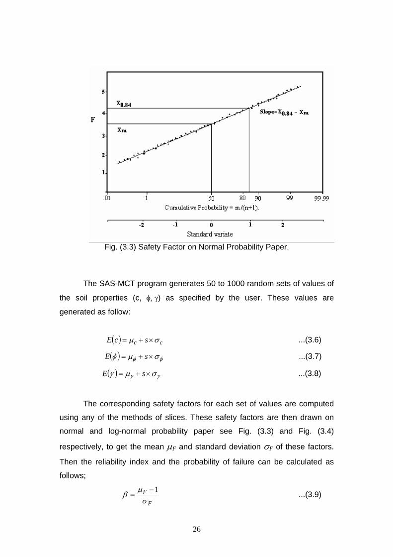
Fig. (3.3) Safety Factor on Normal Probability Paper.
The SAS-MCT program generates 50 to 1000 random sets of values of
the soil properties (c, φ, γ) as specified by the user. These values are
generated as follow:
( ) cc scE σµ ×+= ...(3.6)
( ) φφ σµφ ×+= sE ...(3.7)
( ) γγ σµγ ×+= sE ...(3.8)
The corresponding safety factors for each set of values are computed
using any of the methods of slices. These safety factors are then drawn on
normal and log-normal probability paper see Fig. (3.3) and Fig. (3.4)
respectively, to get the mean µF and standard deviation σF of these factors.
Then the reliability index and the probability of failure can be calculated as
follows;
F
Fσ
µβ 1−= ...(3.9)

27
( ) ( )βφ −=<= 1FpPF ...(3.10)
or
( ) ⎟⎟⎠
⎞⎜⎜⎝
⎛ −=<=
F
FF FpP
σµφ 11 ...(3.11)
where
µF and σF = The mean and the standard deviation of the
safety factor obtained from normal probability
paper.
β = Reliability index.
PF = Probability of failure.
Log-Normal Distribution Generation:
The density function of the log-normal distribution is:
( ) ( )⎥⎥⎦
⎤
⎢⎢⎣
⎡⎟⎟⎠
⎞⎜⎜⎝
⎛ −−=
2ln
21exp
21
ζλ
πζx
xxfX ∞<≤ x0 ...(3.12)
The standard variate (s) based on log-normal distribution is: ( )
ζλ−
=xs ln
….(3.13)
where ( ) 2
21ln ζµλ −= ...(3.14)
⎟⎟⎠
⎞⎜⎜⎝
⎛+= 2
22 1ln
µσζ ...(3.15)

28
Fig. (3.4) Safety Factor on Log-Normal Probability Paper.
The expected value can be derived by solving Eq. (3.12) for x,
( ) ( ) ⎟⎟⎠
⎞⎜⎜⎝
⎛+×+⎟
⎟⎠
⎞⎜⎜⎝
⎛⎟⎟⎠
⎞⎜⎜⎝
⎛+−= 2
2
2
21ln1ln
21lnln
µσ
µσµ sx ….(3.16)
( ) ( )⎥⎥
⎦
⎤
⎢⎢
⎣
⎡
⎟⎟⎠
⎞⎜⎜⎝
⎛+×+⎟
⎟⎠
⎞⎜⎜⎝
⎛⎟⎟⎠
⎞⎜⎜⎝
⎛+−= 2
2
2
21ln1ln
21lnexp
µσ
µσµ sxE ….(3.17)
E(x) = expected value based on log-normal distribution.
Based on Log-Normal distribution the reliability index is,
)1ln(
1)(ln
2
2
2
2
F
F
FF
µσ
µσµ
β
+
⎥⎥⎦
⎤
⎢⎢⎣
⎡+
= ….(3.18)

29
First-Order Second-Moment Approximation
This approach was used by the program SAS-MCT in the search for
maximum probability of failure option. In this approach, the distribution of the
safety factor is not essential and the uncertainty in the safety factor can be
measured by its variance, the performance function (safety factor) can be
described as:
exgF += )( …..(3.19)
Where:
g(x) = the method used in the calculation of the safety factor, which depends
on the geometry and soil properties.
e= modeling error.
Expanding this equation in a Taylor series and trimming to the first
terms yield:
[ ] [ ] [ ]∑∑= =
+∂∂
∂∂
≈k
iji
ji
k
jeVarxxC
xg
xgFVar
1 1, …..(3.20)
where:
[ ] =ji xxC , Covariance of the parameters xi and xj and
[ ] [ ]iji xVxxC =, …..(3.21)
if all the xi and xj are uncorrelated for ji ≠ , then
[ ] [ ] [ ]∑=
+⎟⎟⎠
⎞⎜⎜⎝
⎛∂∂
≈k
ii
ieVarxVar
xgFVar
1
2
…..(3.22)
Making the simplifying assumption that uncertainty in the model error
(e) is uncorrelated with the uncertainties in the model parameters xi and xj.
Equation (3.22) uses the variance (i.e second moment), of the variables, and
it is trimmed to the first-order terms. Hence, the approach is called a first-
order, second-moment method.

30
This approach can be used only with the ordinary method of slices.
Since it is easy to make direct differentiation on the safety factor equation.
Direct differentiation on the other methods is very difficult and complicated.
In order to evaluate the reliability index and the corresponding
probability of failure for each slip surface, the solution of the partial derivatives
of Eq.(3.22) is necessary. According to the ordinary method of slices, for a
slope, the safety factor is defined as,
iii
k
i
k
iiiiii
A
AbCF
αγ
φαγα
sin..
tan.cos..sec..
1
1
′
′′+′
=
∑
∑
=
= …(3.23)
The first-order approximation of the variance of the safety factor in
eq.(3.23) is;
)()()()(222
γγ
φφ
′⎟⎟⎠
⎞⎜⎜⎝
⎛′∂
∂+′⎟⎟
⎠
⎞⎜⎜⎝
⎛′∂
∂+′⎟
⎠⎞
⎜⎝⎛
′∂∂
= VarFVarFCVarCFFVar ...(3.24)
Where
∑
∑
=
=
′=
′∂∂
k
iii
k
iii
A
b
CF
1
1
sin..
sec
αγ
α ...(3.25)
∑
∑
=
=
′
′′
=′∂
∂k
iii
k
iii
A
AF
1
1
2
sin..
sec.cos..
αγ
φαγ
φ ...(3.25)
[ ]
2
1
1
)sin..(
)sin.)(tan.cos..sec..()tansin.)(sin..(
∑
∑
=
=
′
′′+′−′′=
′∂∂
k
iiii
k
iiiiiiiiiiii
A
AAbCAAF
αγ
αφαγαφααγ
γ…(3.26)

31
CHAPTER IV
SAS-MCT PROGRAM
Program Features:
Stability Analysis of Slopes using Monte-Carlo Technique (SAS-MCT4.0)
is a computer software programmed in Microsoft® Visual Basic 6.0 capable of
analyzing stability of man-made or natural slopes under static and earthquake
loading. The most critical slip surface and its corresponding safety factor are
evaluated using Monte-Carlo technique and methods of slices. The main frame
of the program is shown in Fig. (4.1). The program aims at solving the following
problems in slope stability analysis:
1- Two-dimensional analysis of any slope stability configuration
assuming circular slip surface, and using either one of the following
methods- as specified by the user:
a- Ordinary method,
b- Bishop’s method,
c- Janbu’s method,
d- Spencer’s method, and e- Morgenstern-Price method (GLE).
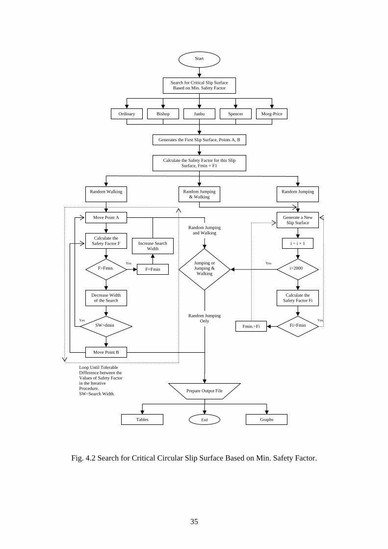
The program aims at evaluating the global minimum safety factor using
Monte Carlo technique. In this respect, the program supports a user friendly
interface wizard for file preparation in which the geometry of slopes, layers,
and the properties of materials are encoded. The program also shows the
critical surface searching routine graphically, and locates the most critical slip
surface. See Fig. (4.2).

32
2- The program can be used to search for the critical circular slip
surface as in point (10 above, but based on maximum probability of failure.
First-order second-moment approximation is used to estimate the probability
of failure (pf). This option is valid for ordinary method. See Fig. (4.3).
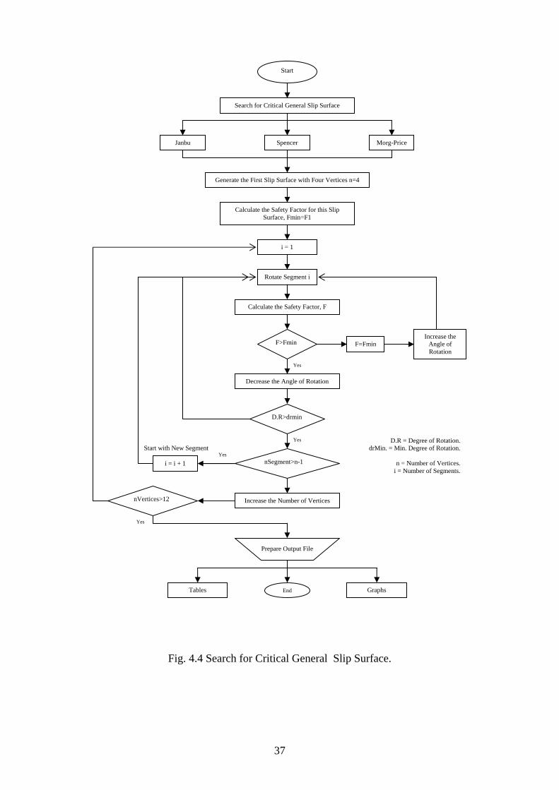
3- Two-dimensional analysis of slope stability assuming irregular slip
surface using one of the following methods;
a- Janbu’s method,
b- Spencer’s method, and
c- Morgenstern-Price method (GLE).
In this respect, the program searches for the most critical slip surface by
representing every trial surface by 4,5,6, …. to 12 vertices trying to simulate the
shape of the real slip surface. The most critical slip surface corresponding to
these vertices will also be shown graphically. See Fig. (4.4).
4- The program also calculates the safety factor for a specified circular
and non-circular slip surfaces.
5- Seismic slope stability analysis using the Pseudo-static method. The
program computes the reduction in the safety factor due to a specified
acceleration input- expressed in percent of ground acceleration (g).
6- Three-dimensional slope stability analysis using one of the
extensions of Bishop’s or Janbu’s two-dimensional methods. The most critical
slip surface will also be shown in three-dimensional view.

33
7- SAS-MCT program user may perform Reliability Analysis. In this
part, the program generates a large number of different expected soil
parameters assuming either normal or log-normal distribution and calculates
the safety factor for each random set. These trails are used to construct the
distribution of the safety factor and the corresponding reliability index (β) and
the probability of failure Pf.
8- Stability analysis can be conducted using either total or effective
parameters.
9- Stability analysis can be conducted using both SI and British units.

34
Fig. 4.1 Main Frame of SAS-MCT Program.
Generation of N Different Values of Soil Properties c, φ, and γ to estimate the Uncertainty in the calculated Safety Factor.
Circular Non-Circular
Start
Prepare Input File
Specified Slip Surface Search for Min. Factor of Safety
Circular Non-Circular
Input Xc,Yc,R Input Vertices See Figure(4.2 and 4.4) See Figure (4.3)
Ordinary Bishop Janbu Spencer Morg-Price
Calculate Factor of Safety
No
Yes
Input Seismic Coefficient
Prepare Output File
No
Yes
Generate New C,Phi,Gama
Prepare Normal Probability Paper
Tables Graphs End
Reliability?
Seismic?
Search for Max. Probability of Failure
Circular Non-Circular
35
Fig. 4.2 Search for Critical Circular Slip Surface Based on Min. Safety Factor.
Yes
Yes
Yes
Yes
Loop Until Tolerable Difference between the Values of Safety Factor in the Iterative Procedure. SW=Search Width. Prepare Output File
Tables Graphs End
Start
Search for Critical Slip Surface Based on Min. Safety Factor
Ordinary Bishop Janbu Spencer Morg-Price
Generates the First Slip Surface, Points A, B
Calculate the Safety Factor for this Slip Surface, Fmin = F1
Random Walking Random Jumping & Walking
Random Jumping
Move Point A
Calculate the Safety Factor F
F>Fmin.
Decrease Width of the Search
SW>dmin
Move Point B
Generate a New Slip Surface
i = i + 1
i>2000
Calculate the Safety Factor Fi
Fi>Fmin
Jumping or Jumping &
Walking F=Fmin
Increase Search Width
Fmin.=Fi
Random Jumping Only
Random Jumping and Walking

36
Fig. 4.3 Search for Critical Circular Slip Surface Based on Max. Probability of
Failure.
Yes
Yes
Yes
Yes
Loop Until Tolerable Difference between the Values of Safety Factor in the Iterative Procedure. SW=Search Width. Prepare Output File
Tables Graphs End
Start
Search for Critical Circular Slip Surface Based on Max. Probability of Failure
Generates the First Slip Surface, Points A, B
Calculate the Probability of Failure for this Slip Surface, PfMax. = Pf1
Random Walking Random Jumping & Walking
Random Jumping
Move Point A
Calculate the Safety Factor F
Pf>Max
Decrease Width of the Search
SW>dmin
Move Point B
Generate a New Slip Surface
i = i + 1
i>2000
Calculate the Prob. of Failure
Pf<Max
Jumping or Jumping &
Walking PfMax=Pf
Increase Search Width
PfMax=Pf
Random Jumping Only
Random Jumping and Walking
Ordinary Method (Only)
Note: The Probability of Failure are Calculated Based on First Order Approximation.
37
Fig. 4.4 Search for Critical General Slip Surface.
Start with New Segment
Yes
Yes
Yes
Yes
Prepare Output File
Tables Graphs End
Start
Search for Critical General Slip Surface
Generate the First Slip Surface with Four Vertices n=4
Calculate the Safety Factor for this Slip Surface, Fmin=F1
F>Fmin
Janbu Spencer Morg-Price
i = 1
Rotate Segment i
Calculate the Safety Factor, F
Decrease the Angle of Rotation
D.R>drmin
Increase the Number of Vertices
i = i + 1
nVertices>12
F=Fmin Increase the
Angle of Rotation
nSegment>n-1
D.R = Degree of Rotation. drMin. = Min. Degree of Rotation.
n = Number of Vertices.
i = Number of Segments.

38
Program Description and Organization:
The program is composed of different classes and modules written in
Microsoft® Visual Basic 6.0. The following are the main subroutines and
functions that are used in the program:
1- Subroutine ORDINARY is used to determine the factor of safety by
Ordinary method, i.e., Fellenius method of slices.
2- Subroutine BISHOP is used to determine the factor of safety by simplified
Bishop’s method of slices.
3- Subroutine JANBU is used to determine the factor of safety using Janbu’s
simplified method of stability analysis.
4- Subroutine SPENCER is used to determine the safety factor via Spencer’s
method of stability analysis.
5- Subroutine MORG is used to determine the factor of safety using
Morganstern-Price method of stability analysis.
6- Subroutine 3DBISH is used to determine the three-dimensional safety
factor for the most critical slip surface observed in two-dimensional analysis
using the extension of Bishop’s two-dimensional analysis.
7- Subroutine 3DJANBU is used to determine the three-dimensional safety
factor for the most critical slip surface observed in two-dimensional analysis
using the extension of Janbu’s two-dimensional analysis.
8- Subroutine JANNON is used to calculate the safety factor for non-circular
slip surface using Janbu’s simplified method of stability.

39
9- Subroutine SPENNON is used to calculate the safety factor for non-
circular slip surface using Spencer’s simplified method of stability for non-
circular slip surface.
10- Subroutine DEVIDER is used to increase the number of vertices of the
critical slip surface by putting a new one in the center of the largest
distance between two adjacent vertices. The subroutine checks that the
new vertex satisfies the boundary condition.
11- Function RAN1 is used to generate random numbers extracted from a
uniformly distributed population in the range [0,1].
12- Function FO is used to calculate the correction factor of Janbu’s
simplified method. This function depends on the relative depth of the
landslide in relation to its length and on the nature of the soil properties.
13- Subroutine NORMAL is used to generate (n) random sets of the
parameters (c, φ, and γ) and to calculate the safety factor for every set of
values, where n varies from 50 to 1000.
14- Subroutine AREANOR is used to calculate the standard normal variate
(gasdev) for the (n) cumulative probabilities generated by Subroutine
NORMAL.
15- Subroutine ZNOR numerically integrates the standard normal
distribution equation using Least Square method.
16- Subroutine PAPER is used to construct the normal probability paper.
17- Subroutine GAWS is used to fit the data in the normal probability
paper.

40
CHAPTER V
Illustrative Examples
Example 1
Description:
This example is taken from Stable5M manual and is analyzed using
Janbu’s method. The safety factor obtained using PC Stable5M is 1.371.
Figure (5.1) shows the cross section and Table (5.1) shows the summary
information for this example. The physical properties of soil layers and the
coordinates of the geometry are shown in Tables (5.2 & 5.3) respectively.
Two cases will be conducted for this example. In Case (I) the slope will
be analyzed assuming circular slip surface, while case (II) assumes a
noncircular slip surface.
Fig. (5.1) Slope Geometry.

41
Table (5.1) Summary Information. Item Case I Case II
Objective of the Search
Find Minimum Safety Factor
Method of Search Janbu’s Method Slip Surface Circular Non-Circular Type of Analysis 3-Dimension 2-Dimension Type of Search Random Jumping --- Stress Analysis Type Effective Stress Search Limits (3.5-62.5) m No. of Layers 3 Layers No. of Slices 50 Slices Unit Weight of Water 9.81 kN/mP
3P
Existence of Water Table
Water Table
Storage Type Not Filled Existence of Stiff Layer Stiff Layer (Bearing Stratum) Existence of Cracks No Cracks Reliability Analysis Not Required Seismic Data Static Analysis External Loads No External Loads Table (5.2) Soil Properties.
Layer No. Description φ (P
oP) C
(kN/m P
2P)
γ (kN/m P
3P)
1 Layer 1 0 0.00 18.30 2 Layer 2 14 23.94 18.30 3 Layer 3 14 23.94 19.52
Table (5.3) Geometry. Layer 1 Layer 2 Layer 3
X Y X Y X Y 0.00 20.73 0.00 20.73 0.00 20.736.71 20.42 6.71 20.42 6.71 20.42
11.58 19.20 11.58 19.20 11.58 19.2030.80 26.83 30.80 26.83 19.20 22.5042.07 31.40 62.50 30.18 25.30 23.7862.50 33.53 31.71 25.00
37.20 25.91 42.68 26.52 62.50 28.35

42
File Preparation: Open SAS-MCT program, on the File menu click “New”, the
browser will appear that requests you to specify the path of the file to
be created. Input wizard screen will appear as shown in Figure (5.2).
Fig. (5.2) Input Wizard.
UGeneral TabU: Contains general information about the project. Feel free to
fill in this information (Optional Information). Then, click Next button to move
into objective tab as shown in Figure (5.3).

43
Fig. (5.3) Objective Tab.
UObjective Tab U: In this tab the user will be prompted to specify the
objective of the search and the slip surface mechanism. The objective of
the search will be one the following three options:
1. Minimum Safety Factor: This option can be used when
minimum safety factor is required.
2. Maximum Probability of Failure: First-order second moment
approximation is used to estimate the reliability index (β).
(Note: Maximum Probability of Failure can be used only with
the Ordinary method.)

44
3. Safety Factor for a Specified Slip Surface: This option can be
used when the user wants to calculate the safety factor for a
slope with a predefined slip surface.
For the slip surface mechanism, the user can either use a circular or a
noncircular slip surface. (Note: When calculating the safety factor for a
specified slip surface, the user will be prompted to enter the radius, x-
coordinates, and y-coordinates for the circular slip surfaces. Otherwise,
the x & y coordinates will be defined for the noncircular slip surface.)
In this example, the aim is to find the minimum safety factor with
circular slip surface (Case I) and the minimum noncircular slip surface
(Case II). Click Circular Slip Surface, then, click next button to move into
method tab as shown in Figure (5.4).
Fig. (5.4) Method Tab.
U

45
Method Tab U: Five common methods of stability analysis can be used
for the simulation process, these are:
1. Ordinary Method.
2. Bishop’s Method.
3. Janbu’s Method.
4. Spencer’s Method.
5. Morgenstern-Price’s Method.
When using Morgenstern-Price’s method, the user has to specify the
Morgenstern-Price function option that will be used, see Figure (5.5) and
these options are as follows:
1. Constant Function.
2. Half-Sine Function.
3. Clipped-Sine Function.
4. User-Specified Function.
Note: Ordinary and Bishop’s methods are not valid for noncircular slip
surface analysis.
In this example, use Janbu’s method, then click Next button to move
into options tab as shown in Figure (5.6).

46
Fig. (5.5) Types of Functions Used for Morgenstern-Price’s Method.

47
Fig. (5.6) Options Tab.
UOptions TabU: In this tab the user must specify the desired options such
as:
1. Type of Analysis: 2-dimensional analysis or 3-dimensional
analysis (Note: 3-dimensional analysis is only valid for
circular slip surfaces), in this example case I select 3-
dimensional analysis, and for case II select 2-dimensional
analysis.
2. Type of Search: (only for circular slip surface) The user might
choose one of the three types of search: random jumping,
random walking, or both random jumping and walking. Select
the random jumping option.
48
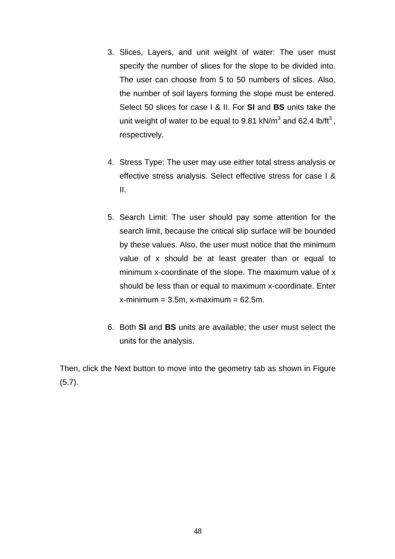
3. Slices, Layers, and unit weight of water: The user must
specify the number of slices for the slope to be divided into.
The user can choose from 5 to 50 numbers of slices. Also,
the number of soil layers forming the slope must be entered.
Select 50 slices for case I & II. For SI and BS units take the
unit weight of water to be equal to 9.81 kN/mP
3P and 62.4 lb/ftP
3 P,
respectively.
4. Stress Type: The user may use either total stress analysis or
effective stress analysis. Select effective stress for case I &
II.
5. Search Limit: The user should pay some attention for the
search limit, because the critical slip surface will be bounded
by these values. Also, the user must notice that the minimum
value of x should be at least greater than or equal to
minimum x-coordinate of the slope. The maximum value of x
should be less than or equal to maximum x-coordinate. Enter
x-minimum = 3.5m, x-maximum = 62.5m.
6. Both SI and BS units are available; the user must select the
units for the analysis.
Then, click the Next button to move into the geometry tab as shown in Figure
(5.7).
49
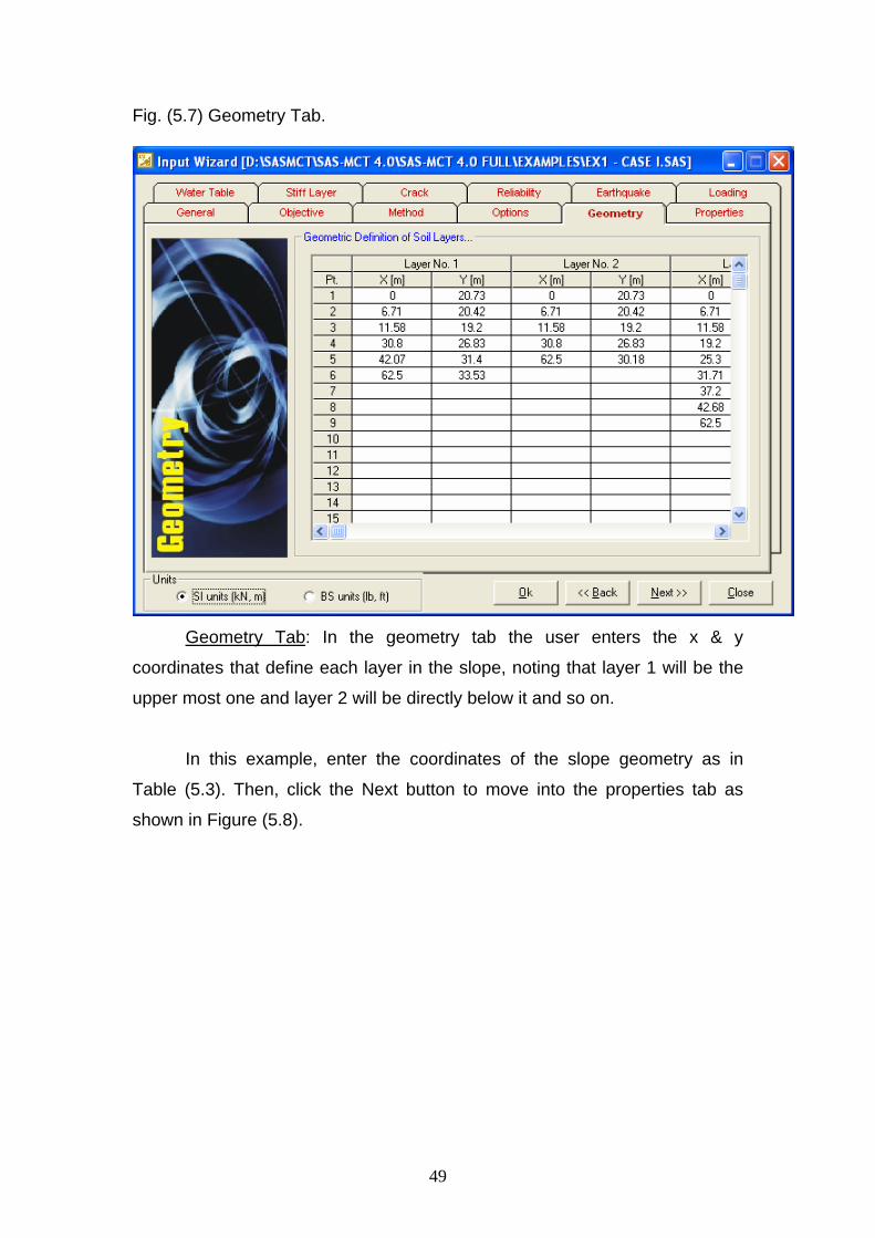
Fig. (5.7) Geometry Tab.
UGeometry TabU: In the geometry tab the user enters the x & y
coordinates that define each layer in the slope, noting that layer 1 will be the
upper most one and layer 2 will be directly below it and so on.
In this example, enter the coordinates of the slope geometry as in
Table (5.3). Then, click the Next button to move into the properties tab as
shown in Figure (5.8).
50
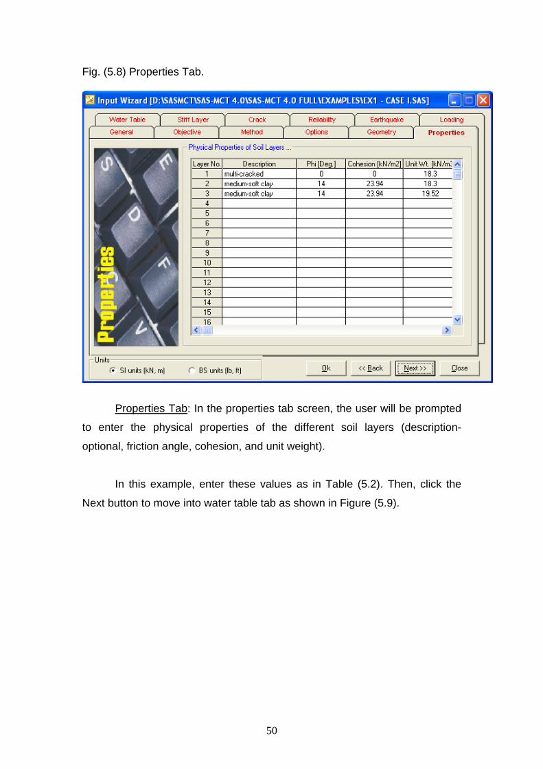
Fig. (5.8) Properties Tab.
UProperties TabU: In the properties tab screen, the user will be prompted
to enter the physical properties of the different soil layers (description-
optional, friction angle, cohesion, and unit weight).
In this example, enter these values as in Table (5.2). Then, click the
Next button to move into water table tab as shown in Figure (5.9).

51
Fig. (5.9) Water Table Tab.
UWater Table TabU: In this tab the user must specify whether there is a
water table or not simply by clicking on the check box beside the Existence of
Water Table field. The user may skip this screen if there is no water table.
Otherwise, the user should specify whether it is the water table or the pore
water pressure ratio option. Also, should specify the storage type whether
filled with water or not. When the storage is filled with water, the user will be
prompted to enter the x-intersection of water level with the topography, see
Figure (5.10).

52
Fig. (5.10) Storage Filled with Water.
In this example, no water storage is chosen and water table option is used.
Enter the coordinates of the layer that define the water table as shown in
Figure (5.10). Then, click the Next button to move into Stiff layer tab as shown
in Figure (5.11).

53
Fig. (5.11) Stiff Layer Tab.
UStiff Layer TabU: In this tab the user must specify whether there is a stiff
layer or not simply by clicking on the check box beside the Existence of Stiff
Layer field. The user may skip this screen if there is no stiff layer. Otherwise,
the user should enter the coordinates that define the stiff layer.
In our example, a stiff layer exists and is defined by the coordinates as
shown in Figure (5.11). Then, click the Next button to move into the crack tab
as shown in Figure (5.12).

54
Fig. (5.12) Crack Tab.
UCrack TabU: In this tab, the user is asked to specify whether there is a
cracked layer or not. The user may skip this screen if there is no cracked
layer. Otherwise, the user will be prompted to enter the x-position of crack and
its depth, see Figure (5.13a), and whether it is filled with water or not. It is
worthy to say that if there is a cracked layer (layer with multi cracks), see
Figure (5.13b), the user may skip this screen and consider this layer as a
layer with a friction angle and cohesion equal to zero (i.e.: φ=0, c=0).

55
a- Single Crack.
b- Multi Cracks.
Fig. (5.13) Presence of Cracks.

56
In this example, skip this screen to the reliability tab as shown in Figure
(5.14).
Fig. (5.14) Reliability Tab.
UReliability Tab U: The user may use this screen when reliability analysis
is required, and the number of generation data must be entered. Also, the
standard deviation for the friction angle, cohesion, and unit weight, for each
soil layer, must be supplied.
In this example, reliability analysis is not required, so skip this screen
by clicking the Next button to move into the earthquake tab as shown in
Figure (5.15).

57
Fig. (5.15) Earthquake Tab.
UEarthquake TabU: In the earthquake tab, the user is asked to specify
the seismic data by choosing either static or earthquake analysis. When
earthquake analysis is required, seismic coefficient as a percent of gravity
acceleration should be entered.
In our example, static analysis is conducted by clicking on static
option. Then click the Next button and move into the last tab in the input
wizard, the loading tab, as shown in Figure (5.16).
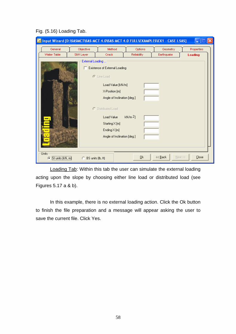
58
Fig. (5.16) Loading Tab.
ULoading Tab U: Within this tab the user can simulate the external loading
acting upon the slope by choosing either line load or distributed load (see
Figures 5.17 a & b).
In this example, there is no external loading action. Click the Ok button
to finish the file preparation and a message will appear asking the user to
save the current file. Click Yes.

59
a- Line Load Option.
b- Distributed Load Option.
Fig. (5.17) Presence of External Loading.

60
After completing the file preparation, click on the View menu >> Graphs
>> Slope Geometry to see the slope. After that, it is time for slope stability
processing. This can simply occur by clicking on Process menu >> Start or
(press F5). A screen will appear showing that the analysis process is in
progress (see Figure 5.18).
Fig. (5.18) SAS-MCT Running Screen.
61
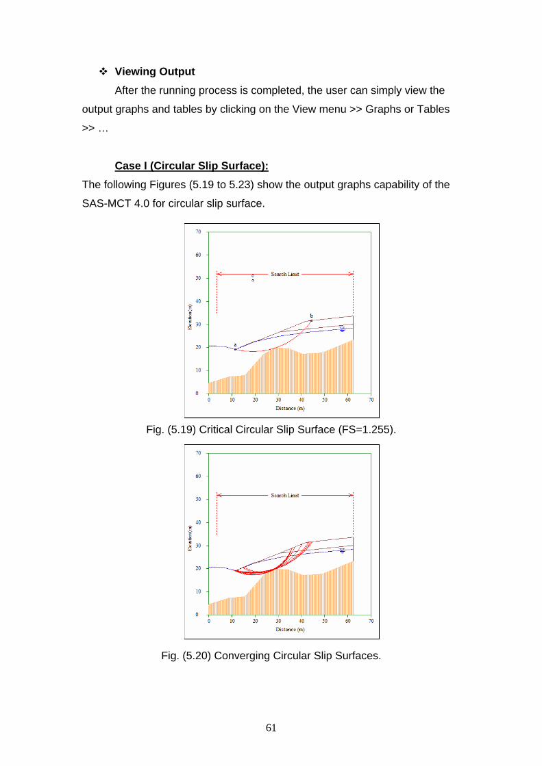
Viewing Output After the running process is completed, the user can simply view the
output graphs and tables by clicking on the View menu >> Graphs or Tables
>> …
UCase I (Circular Slip Surface): The following Figures (5.19 to 5.23) show the output graphs capability of the
SAS-MCT 4.0 for circular slip surface.
Fig. (5.19) Critical Circular Slip Surface (FS=1.255).
Fig. (5.20) Converging Circular Slip Surfaces.

62
Fig. (5.21) All Tested Circular Slip Surfaces.
Fig. (5.22) 3-Dimensional Circular Slip Surface (FS=1.791).
63
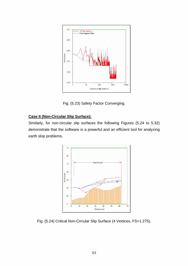
Fig. (5.23) Safety Factor Converging.
UCase II (Non-Circular Slip Surface):U
Similarly, for non-circular slip surfaces the following Figures (5.24 to 5.32)
demonstrate that the software is a powerful and an efficient tool for analyzing
earth slop problems.
Fig. (5.24) Critical Non-Circular Slip Surface (4 Vertices, FS=1.275).

64
Fig. (5.25) Critical Non-Circular Slip Surface (5 Vertices, FS=1.256).
Fig. (5. 26) Critical Non-Circular Slip Surface (6 Vertices, FS=1.256).

65
Fig. (5.27) Critical Non-Circular Slip Surface (7 Vertices, FS=1.243).
Fig. (5.28) Critical Non-Circular Slip Surface (8 Vertices, FS=1.237).

66
Fig. (5.29) Critical Non-Circular Slip Surface (9 Vertices, FS=1.237).
Fig. (5.30) Critical Non-Circular Slip Surface (10 Vertices, FS=1.237).

67
Fig. (5.31) Critical Non-Circular Slip Surface (11 Vertices, FS=1.236).
Fig. (5.32) Critical Non-Circular Slip Surface (12 Vertices, FS=1.224).
68
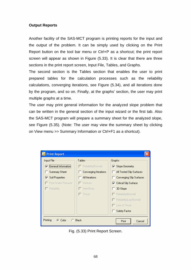
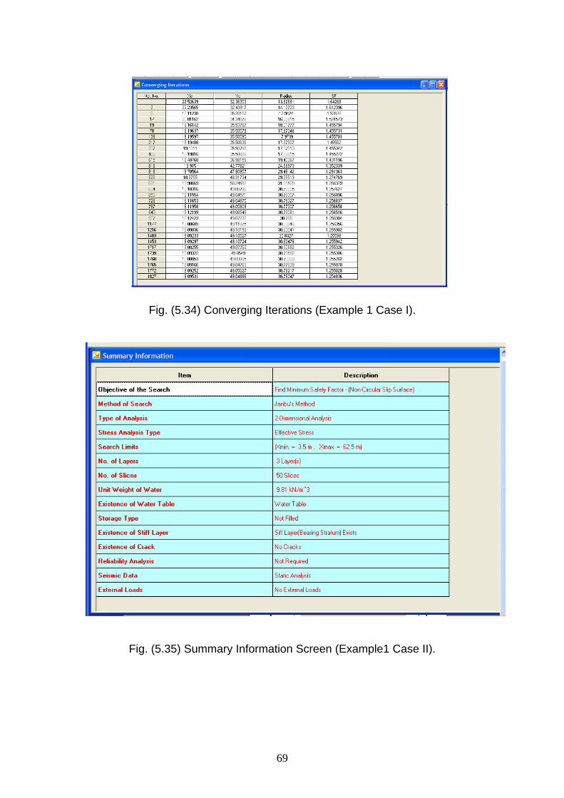
Output Reports Another facility of the SAS-MCT program is printing reports for the input and
the output of the problem. It can be simply used by clicking on the Print
Report button on the tool bar menu or Ctrl+P as a shortcut; the print report
screen will appear as shown in Figure (5.33). It is clear that there are three
sections in the print report screen, Input File, Tables, and Graphs.
The second section is the Tables section that enables the user to print
prepared tables for the calculation processes such as the reliability
calculations, converging iterations, see Figure (5.34), and all iterations done
by the program, and so on. Finally, at the graphs’ section, the user may print
multiple graphs at a time.
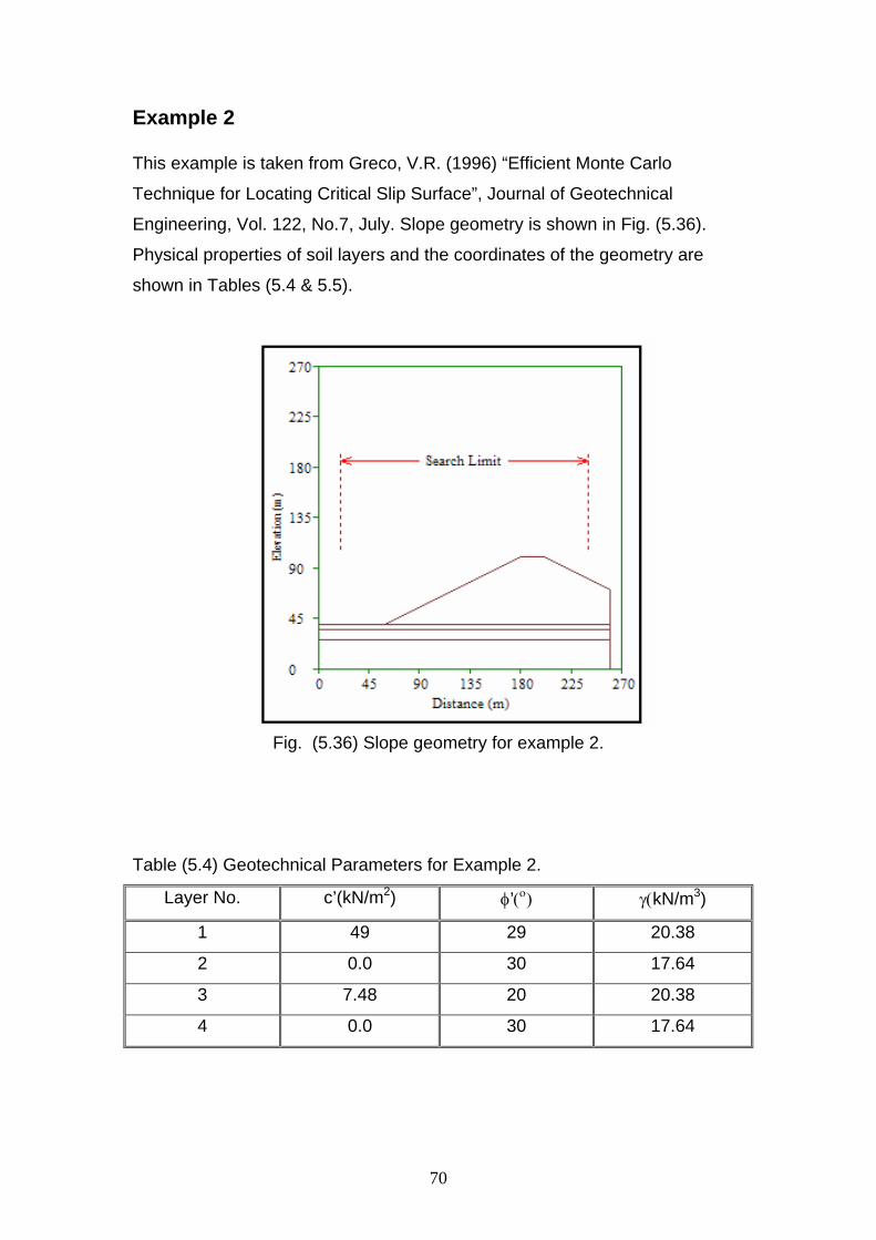
The user may print general information for the analyzed slope problem that
can be written in the general section of the input wizard or the first tab. Also
the SAS-MCT program will prepare a summary sheet for the analyzed slope,
see Figure (5.35). (Note: The user may view the summary sheet by clicking
on View menu >> Summary Information or Ctrl+F1 as a shortcut).
Fig. (5.33) Print Report Screen.
69
Fig. (5.34) Converging Iterations (Example 1 Case I).
Fig. (5.35) Summary Information Screen (Example1 Case II).
70
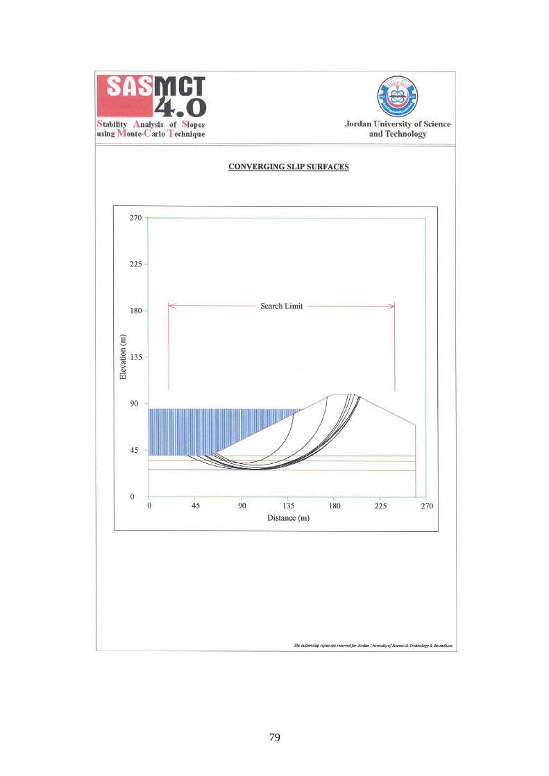
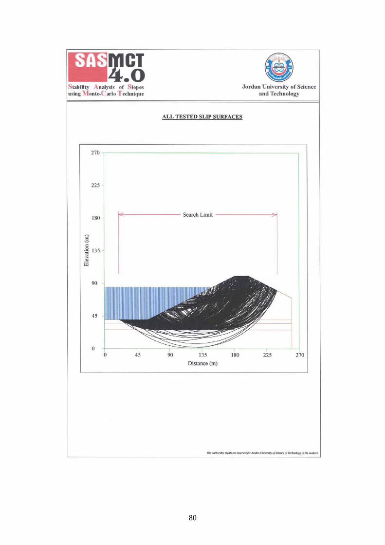
Example 2 This example is taken from Greco, V.R. (1996) “Efficient Monte Carlo
Technique for Locating Critical Slip Surface”, Journal of Geotechnical
Engineering, Vol. 122, No.7, July. Slope geometry is shown in Fig. (5.36).
Physical properties of soil layers and the coordinates of the geometry are
shown in Tables (5.4 & 5.5).
Fig. (5.36) Slope geometry for example 2.
Table (5.4) Geotechnical Parameters for Example 2.
Layer No. c’(kN/mP
2P) φ’( P
οP) γ(kN/mP
3P)
1 49 29 20.38
2 0.0 30 17.64
3 7.48 20 20.38
4 0.0 30 17.64

71
Table (5.5) Cross Section Geometry.
Layer 1 Layer 2 Layer 3 Layer 4
X y x y x y x y
0.0 40.0 0.0 40.0 0.0 35.0 0.0 26.0
60.0 40.0 260.0 40.0 260.0 35.0 260.0 26.0
180.0 100.0
200.0 100.0
260.0 70.0
Several authors analyzed this example and Greco, (1996) summarized their
results along with his results and they are given in Table (5.6) below. This
example is further analyzed using SAS-MCT4.0 program. Different types of
analysis with different cases of loading are used. The results of the analyzed
slope are presented herein after.
Table (5.6) Summary Results using Different Search Methods. Method Factor of Safety
BFGS
DFP
Powell
Simplex
1.423
1.453
1.402
1.405
Pattern Search
Monte Carlo
1.400
1.401
Range of values of safety factors for slip surfaces Method
4 vertices 7 vertices 13 vertices
Pattern Search
Monte Carlo
1.438-1.775
1.437-1.625
1.406-1.421
1.407-1.431
1.4-1.406
1.4-1.413

72
Output for Example No. 2, Case I Circular Slip Surface

73

74

75

76

77

78
79
80

81
82
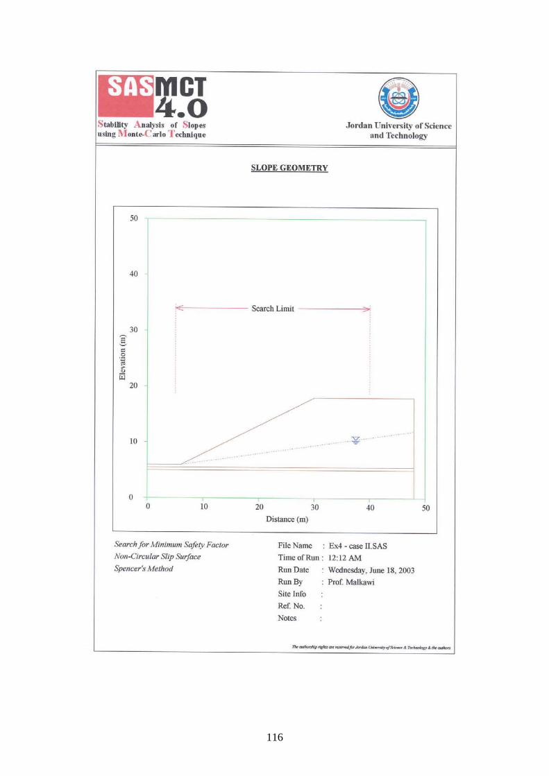
Output for Example No. 2, Case II Non-Circular Slip Surface with Earthquake Loading

83

84

85

86

87
Output for Example No. 2, Case III Specified Slip Surface, Line of Thrust

88

89

90

91

92

93

94

95
Example 3
Karameh dam is situated in the Dead Sea Rift and it is built on deep
soft compressible deposits. Fig. (5.37) presents the cross section. Tables (5.7
and 5.8) show the slope geometry and the soil parameters for the dam.
Fig. (5.37) Cross Section of Karameh Dam.
Table (5.7) Cross Section Geometry.
Layer 1 Layer 2 Layer 3 Layer 4 Layer 5 Layer 6
x Y X y x y x Y x y x Y
0.0 57.0 0.0 57.0 0.0 57.0 0.0 40.0 0.0 39.0 0.0 22.0
83.0 60.0 83.0 60.0 57.0 60.0 140.0 40.0 140.0 39.0 230.0 22.0
143.0 80.0 143.0 80.0 77.0 50.0 145.0 80.0 145.0 34.0
157.0 80.0 157.0 80.0 141.0 50.0 157.0 80.0 157.0 34.0
217.0 59.0 167.0 77.0 145.0 80.0 162.0 39.0 162.0 39.0
230.0 59.0 173.0 42.0 157.0 80.0 230.0 39.0 230.0 39.0
230.0 42.0 162.0 39.0
230.0 39.0

96
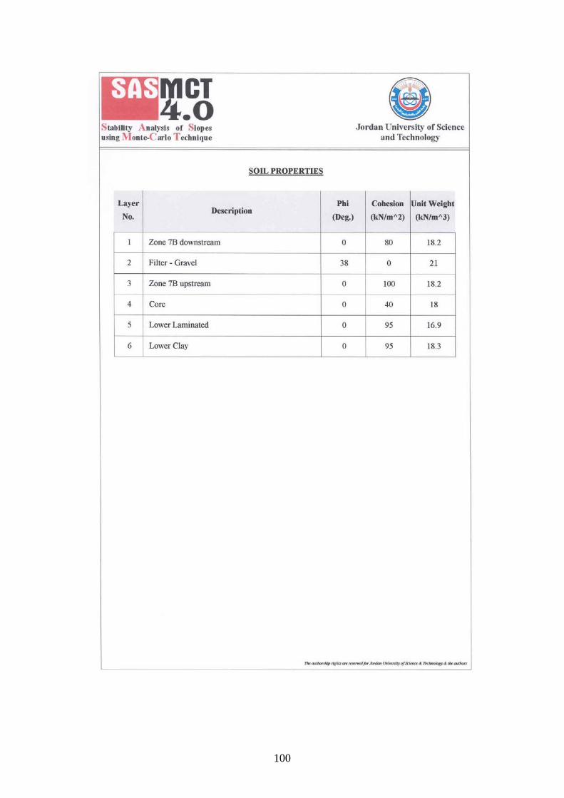
Table (5.8) Soil Properties for Karameh Dam Project.
No. Description γ (kN/mP
3P) c’ (kN/mP
2P) φ’
1 Zone 7B Downstream 18.2 80.0 0.0 2 Filter/ Gravel 21.0 0.0 38.0 3 Zone 7B Upstream 18.2 100.0 0.0 4 Core 18.0 40.0 0.0 5 Lower Laminated 16.9 95.0 0.0 6 Lower Clay 18.3 95.0 0.0
This example was analyzed using SAS-MCT 4.0. The results are
shown below.

97
Output for Example No. 3 Circular Slip Surface

98

99
100

101

102

103

104
Example 4 Example 4 is a homogeneous slope with the presence of a weak thin layer.
This example was originally used by Fredlund and Krahn (1977). Fig. (5.38)
shows the cross section of the analyzed slope. Tables (5.9 and 5.10) show
the coordinates of slope and properties of the soil layers, respectively.
Fig. (5.38) Shows the Cross Section for Example 4.
This example is analyzed using SAS-MCT 4.0. Several loading conditions
were considered, such as line load, uniformly distributed load, crack option
etc. Several illustrative plots are enclosed.

105
Table (5.9) Cross Section Geometry for Example 4.
Layer 1 Layer 2 Layer 3 Water Table
x Y x Y x y x y
0.0 6.0 0.0 5.5 0.0 5.0 0.0 6.0
6.0 6.0 48.0 5.5 48.0 5.0 6.0 6.0
30.0 18.0 48.0 12.0
48.0 18.0
Table (5.10) Geotechnical Soil Properties for Example 4.
Layer No. γ (kN/mP
3P) c’ (kN/mP
2P) φ’
1 18.8 29.0 20.0 2 18.8 0.0 7.0 3 18.8 29.0 20.0

106
Output for Example No. 4, Case I Circular Slip Surface

107

108

109

110

111

112

113
Output for Example No. 4, Case II Non-Circular Slip Surface

114

115
116

117
118
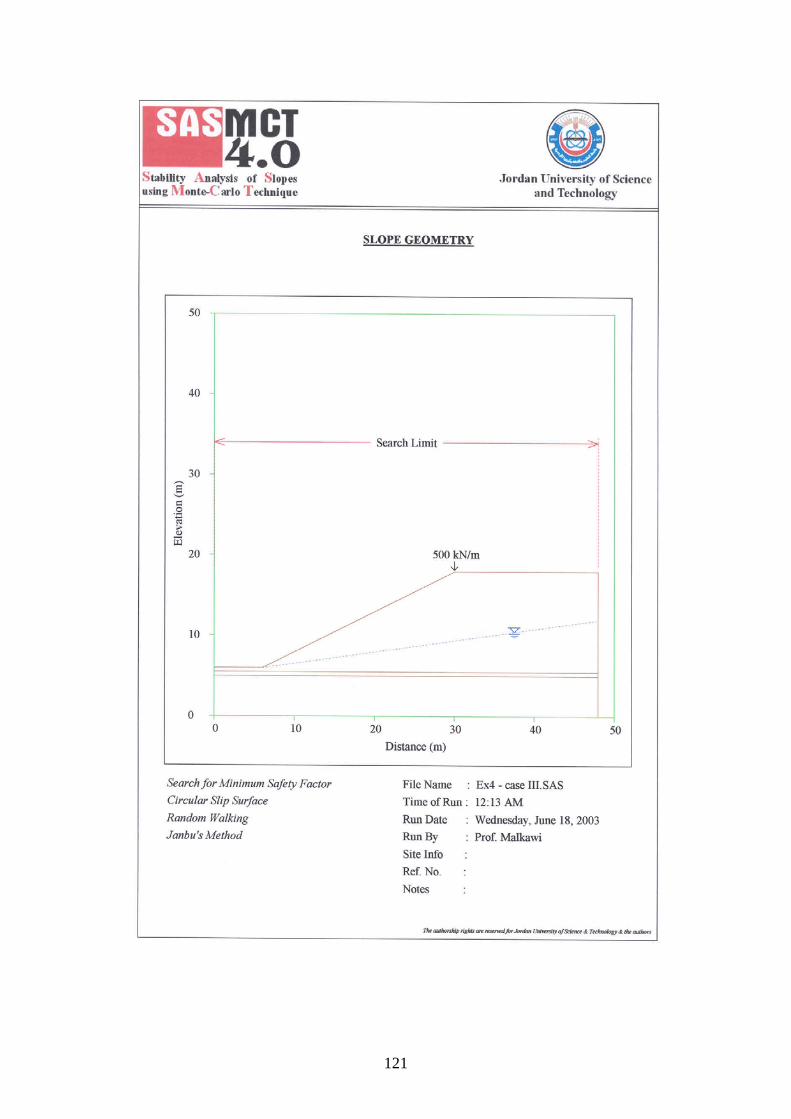
Output for Example No. 4, Case III Circular Slip Surface with Line Load

119

120
121

122

123
Output for Example No. 4, Case IV Non-Circular Slip Surface, Existence of Crack

124

125

126

127

128
Output for Example No. 4, Case V Non-Circular Slip Surface, Distributed Load

129

130

131

132

133

134
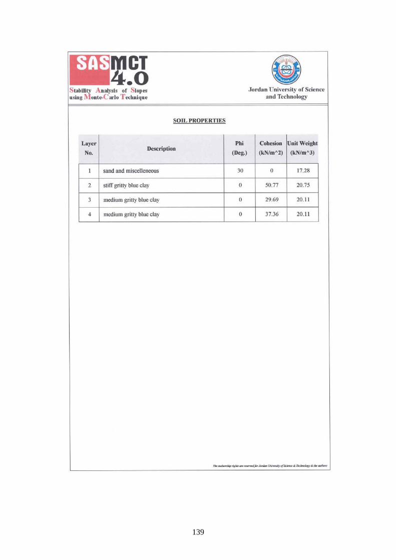
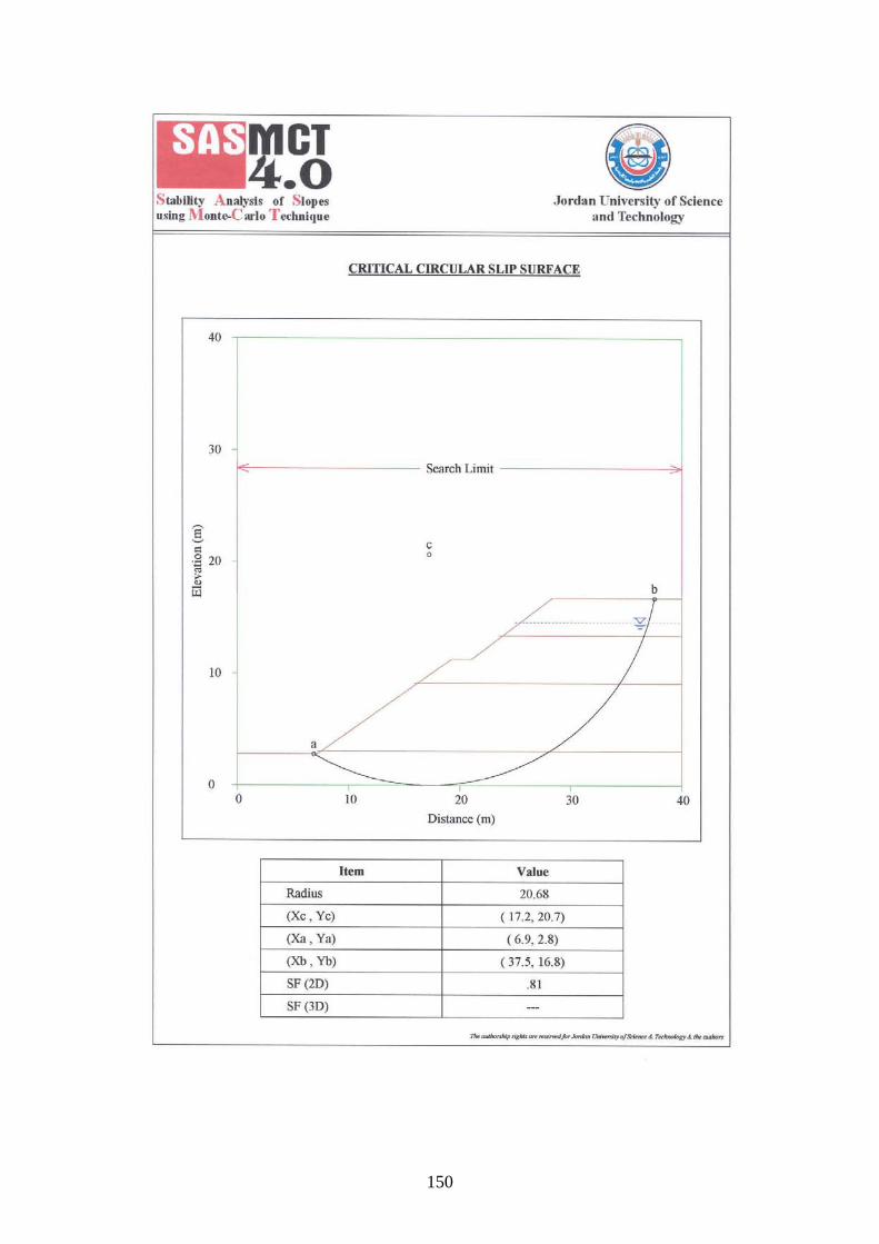
Example 5
This landslide occurred in 1952 during the construction of Congress Street in
Chicago, the north side. Fig. (5.39) shows the cross section of the Congress
street project and Tables (5.11 and 5.12) present the statistical values for the
shear strength parameters and slope coordinates, respectively.
Fig. (5.39) Shows the Cross-Section for Example 5.

135
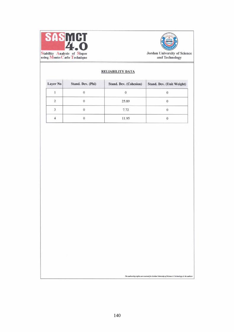
Table (5.11) Statistical Values for the Undrained Strengths at the Congress
Street Project.
Material Type Mean value
(µ)
Standard
Deviation (σ)
Coefficient of
variation (%)
γ (kN/mP
3P) 12.28 n/a n/a
φBu B ( P
oP) 30.0 0.0 0.0
Sand and
miscellaneous
fill (1) CBu B (kN/mP
2P) 0.0 0.0 0.0
γ (kN/mP
3P) 20.75 n/a n/a
φBu B ( P
oP) 0.0 0.0 0.0
Stiff gritty blue
clay (upper
layer) (2) CBu B (kN/mP
2P) 50.77 25.89 51.0
γ (kN/mP
3P) 20.11 n/a n/a
φBu B ( P
oP) 0.0 0.0 0.0
Medium gritty
blue clay
(middle clay)
(3) CBu B (kN/mP
2P) 29.69 7.72 26.0
γ (kN/mP
3P) 20.11 n/a n/a
φBu B ( P
oP) 0.0 0.0 0.0
Medium gritty
blue clay
(middle layer)
(4) CBu B (kN/mP
2P) 37.36 11.95 32.0
Table (5.12) Slope Coordinates.
Layer 1 Layer 2 Layer 3 Layer 4 Water
Table
x y x y X Y x y x y
0.0 2.8 23.5 13.411 15.9 9.144 7.16 3.05 25.0 14.6
7.16 2.8 40.0 13.411 40.0 9.14 40.0 3.05 40.0 14.6
19.2 11.277
21.03 11.277
28.3 16.760
40.0 16.760

136
Output for Example No. 5, Case I Search Based on Minimum Factor of Safety
(Janbu Method)

137

138
139
140

141

142

143

144

145

146
Example No. 5, Case Ia
Search Based on Minimum Factor of Safety
(Ordinary Method)

147

148

149
150
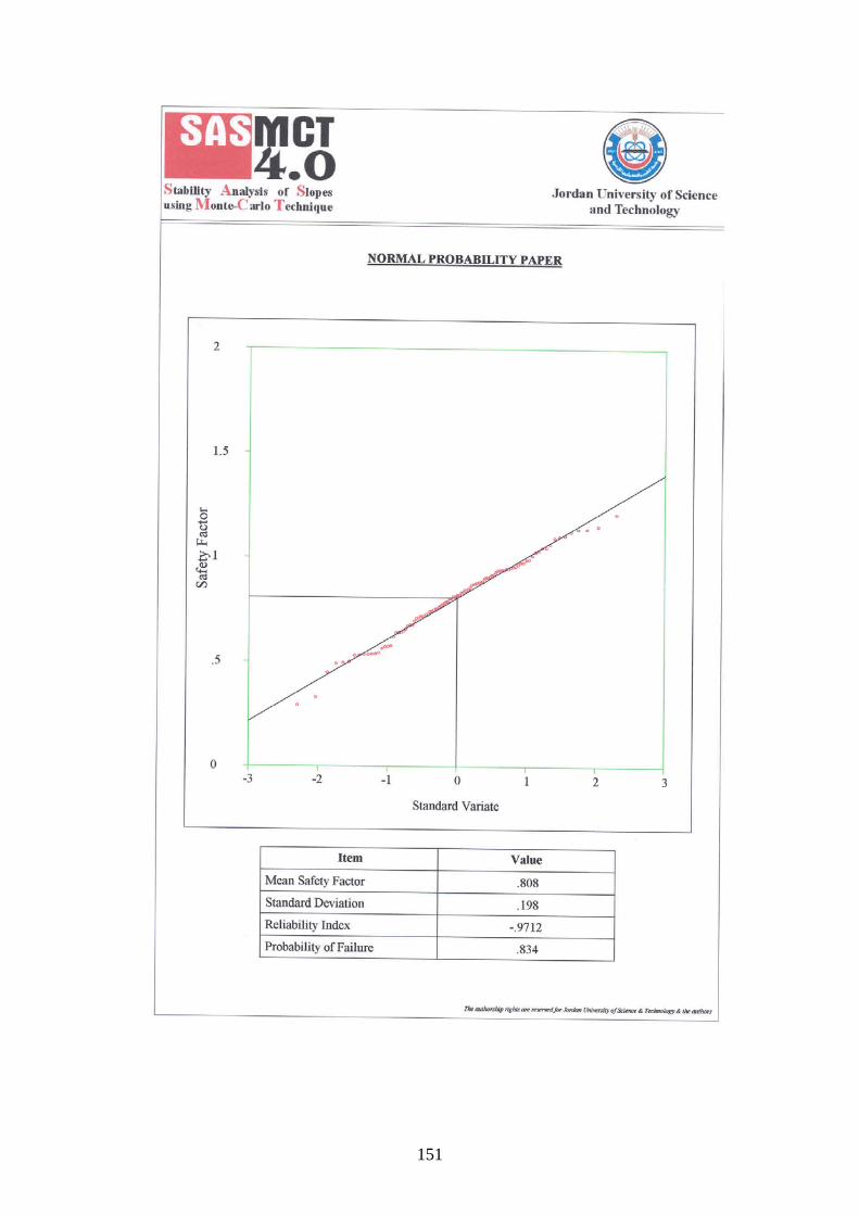
151

152

153
Output for Example No. 5, Case II Search Based on Maximum Probability of Failure

154
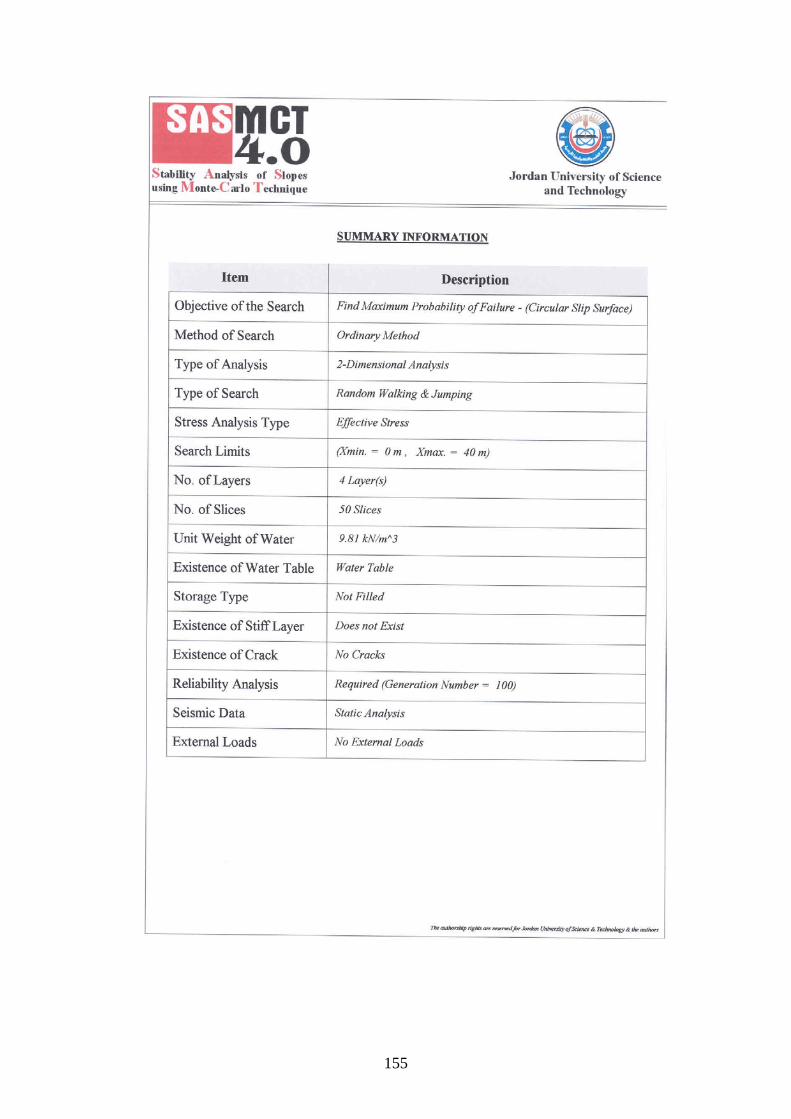
155

156

157
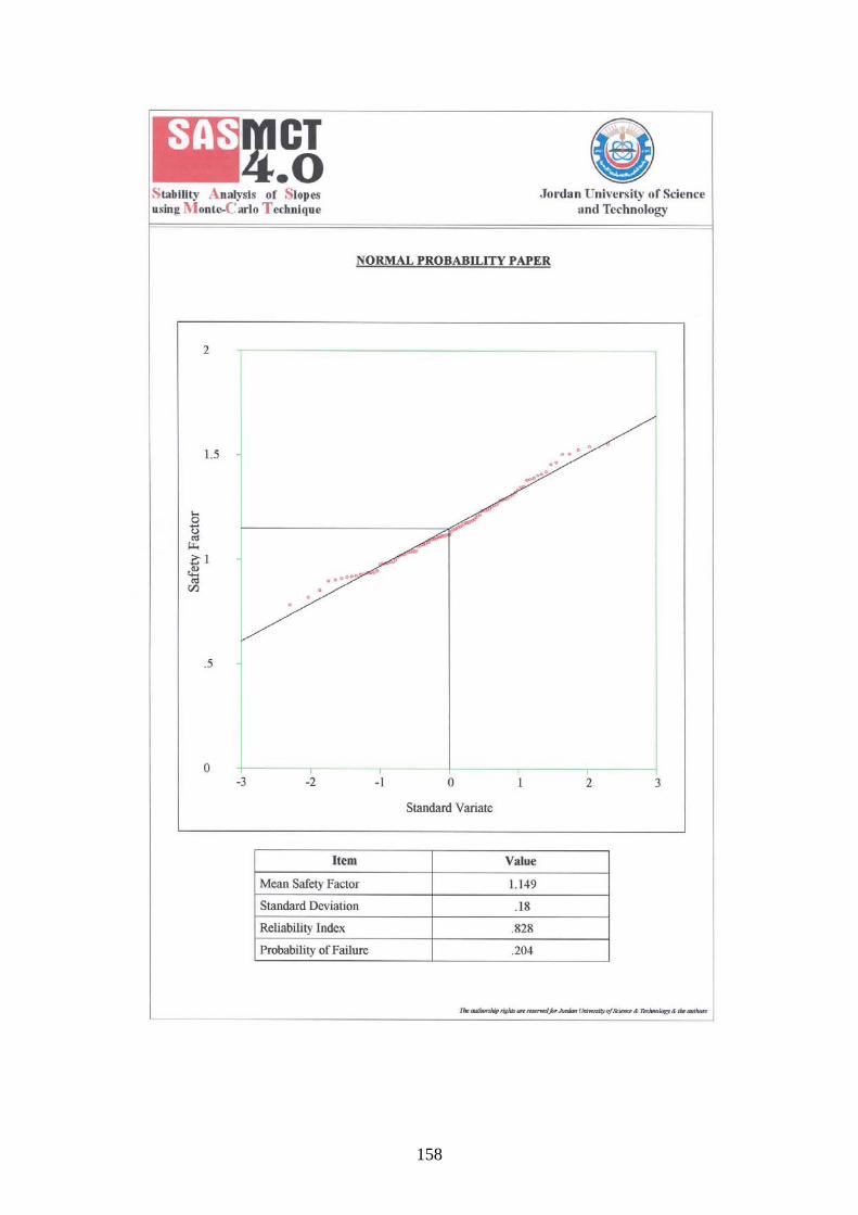
158

159


