SAS/ETS 15.1 User’s Guide
160
SAS/ETS ® 15.1 User’s Guide The AUTOREG Procedure
Transcript of SAS/ETS 15.1 User’s Guide
SAS/ETS® 15.1User’s GuideThe AUTOREG Procedure

This document is an individual chapter from SAS/ETS® 15.1 User’s Guide.
The correct bibliographic citation for this manual is as follows: SAS Institute Inc. 2018. SAS/ETS® 15.1 User’s Guide. Cary, NC:SAS Institute Inc.
SAS/ETS® 15.1 User’s Guide
Copyright © 2018, SAS Institute Inc., Cary, NC, USA
All Rights Reserved. Produced in the United States of America.
For a hard-copy book: No part of this publication may be reproduced, stored in a retrieval system, or transmitted, in any form or byany means, electronic, mechanical, photocopying, or otherwise, without the prior written permission of the publisher, SAS InstituteInc.
For a web download or e-book: Your use of this publication shall be governed by the terms established by the vendor at the timeyou acquire this publication.
The scanning, uploading, and distribution of this book via the Internet or any other means without the permission of the publisher isillegal and punishable by law. Please purchase only authorized electronic editions and do not participate in or encourage electronicpiracy of copyrighted materials. Your support of others’ rights is appreciated.
U.S. Government License Rights; Restricted Rights: The Software and its documentation is commercial computer softwaredeveloped at private expense and is provided with RESTRICTED RIGHTS to the United States Government. Use, duplication, ordisclosure of the Software by the United States Government is subject to the license terms of this Agreement pursuant to, asapplicable, FAR 12.212, DFAR 227.7202-1(a), DFAR 227.7202-3(a), and DFAR 227.7202-4, and, to the extent required under U.S.federal law, the minimum restricted rights as set out in FAR 52.227-19 (DEC 2007). If FAR 52.227-19 is applicable, this provisionserves as notice under clause (c) thereof and no other notice is required to be affixed to the Software or documentation. TheGovernment’s rights in Software and documentation shall be only those set forth in this Agreement.
SAS Institute Inc., SAS Campus Drive, Cary, NC 27513-2414
November 2018
SAS® and all other SAS Institute Inc. product or service names are registered trademarks or trademarks of SAS Institute Inc. in theUSA and other countries. ® indicates USA registration.
Other brand and product names are trademarks of their respective companies.
SAS software may be provided with certain third-party software, including but not limited to open-source software, which islicensed under its applicable third-party software license agreement. For license information about third-party software distributedwith SAS software, refer to http://support.sas.com/thirdpartylicenses.
Chapter 8
The AUTOREG Procedure
ContentsOverview: AUTOREG Procedure . . . . . . . . . . . . . . . . . . . . . . . . . . . . . . . 312Getting Started: AUTOREG Procedure . . . . . . . . . . . . . . . . . . . . . . . . . . . . 314
Regression with Autocorrelated Errors . . . . . . . . . . . . . . . . . . . . . . . . . 314Forecasting Autoregressive Error Models . . . . . . . . . . . . . . . . . . . . . . . . 321Testing for Autocorrelation . . . . . . . . . . . . . . . . . . . . . . . . . . . . . . . 322Stepwise Autoregression . . . . . . . . . . . . . . . . . . . . . . . . . . . . . . . . . 325Testing for Heteroscedasticity . . . . . . . . . . . . . . . . . . . . . . . . . . . . . . 327Heteroscedasticity and GARCH Models . . . . . . . . . . . . . . . . . . . . . . . . . 331
Syntax: AUTOREG Procedure . . . . . . . . . . . . . . . . . . . . . . . . . . . . . . . . . 335Functional Summary . . . . . . . . . . . . . . . . . . . . . . . . . . . . . . . . . . . 335PROC AUTOREG Statement . . . . . . . . . . . . . . . . . . . . . . . . . . . . . . 339BY Statement . . . . . . . . . . . . . . . . . . . . . . . . . . . . . . . . . . . . . . 340CLASS Statement . . . . . . . . . . . . . . . . . . . . . . . . . . . . . . . . . . . . 341MODEL Statement . . . . . . . . . . . . . . . . . . . . . . . . . . . . . . . . . . . . 341HETERO Statement . . . . . . . . . . . . . . . . . . . . . . . . . . . . . . . . . . . 360NLOPTIONS Statement . . . . . . . . . . . . . . . . . . . . . . . . . . . . . . . . . 362OUTPUT Statement . . . . . . . . . . . . . . . . . . . . . . . . . . . . . . . . . . . 363RESTRICT Statement . . . . . . . . . . . . . . . . . . . . . . . . . . . . . . . . . . 365TEST Statement . . . . . . . . . . . . . . . . . . . . . . . . . . . . . . . . . . . . . 366
Details: AUTOREG Procedure . . . . . . . . . . . . . . . . . . . . . . . . . . . . . . . . . 368Missing Values . . . . . . . . . . . . . . . . . . . . . . . . . . . . . . . . . . . . . . 368Autoregressive Error Model . . . . . . . . . . . . . . . . . . . . . . . . . . . . . . . 368Alternative Autocorrelation Correction Methods . . . . . . . . . . . . . . . . . . . . 372GARCH Models . . . . . . . . . . . . . . . . . . . . . . . . . . . . . . . . . . . . . 373Heteroscedasticity- and Autocorrelation-Consistent Covariance Matrix Estimator . . . 379Goodness-of-Fit Measures and Information Criteria . . . . . . . . . . . . . . . . . . 382Testing . . . . . . . . . . . . . . . . . . . . . . . . . . . . . . . . . . . . . . . . . . 385Predicted Values . . . . . . . . . . . . . . . . . . . . . . . . . . . . . . . . . . . . . 409OUT= Data Set . . . . . . . . . . . . . . . . . . . . . . . . . . . . . . . . . . . . . . 413OUTEST= Data Set . . . . . . . . . . . . . . . . . . . . . . . . . . . . . . . . . . . 413Printed Output . . . . . . . . . . . . . . . . . . . . . . . . . . . . . . . . . . . . . . 415ODS Table Names . . . . . . . . . . . . . . . . . . . . . . . . . . . . . . . . . . . . 416ODS Graphics . . . . . . . . . . . . . . . . . . . . . . . . . . . . . . . . . . . . . . 418
Examples: AUTOREG Procedure . . . . . . . . . . . . . . . . . . . . . . . . . . . . . . . 419Example 8.1: Analysis of Real Output Series . . . . . . . . . . . . . . . . . . . . . . 419Example 8.2: Comparing Estimates and Models . . . . . . . . . . . . . . . . . . . . 423

312 F Chapter 8: The AUTOREG Procedure
Example 8.3: Lack-of-Fit Study . . . . . . . . . . . . . . . . . . . . . . . . . . . . . 427Example 8.4: Missing Values . . . . . . . . . . . . . . . . . . . . . . . . . . . . . . 430Example 8.5: Money Demand Model . . . . . . . . . . . . . . . . . . . . . . . . . . 435Example 8.6: Estimation of ARCH(2) Process . . . . . . . . . . . . . . . . . . . . . 439Example 8.7: Estimation of GARCH-Type Models . . . . . . . . . . . . . . . . . . . 443Example 8.8: Illustration of ODS Graphics . . . . . . . . . . . . . . . . . . . . . . . 447
References . . . . . . . . . . . . . . . . . . . . . . . . . . . . . . . . . . . . . . . . . . . 455
Overview: AUTOREG ProcedureThe AUTOREG procedure estimates and forecasts linear regression models for time series data whenthe errors are autocorrelated or heteroscedastic. The autoregressive error model is used to correct forautocorrelation, and the generalized autoregressive conditional heteroscedasticity (GARCH) model and itsvariants are used to model and correct for heteroscedasticity.
When time series data are used in regression analysis, often the error term is not independent through time.Instead, the errors are serially correlated (autocorrelated). If the error term is autocorrelated, the efficiencyof ordinary least squares (OLS) parameter estimates is adversely affected and standard error estimates arebiased.
The autoregressive error model corrects for serial correlation. The AUTOREG procedure can fit autore-gressive error models of any order and can fit subset autoregressive models. You can also specify stepwiseautoregression to select the autoregressive error model automatically.
To diagnose autocorrelation, the AUTOREG procedure produces generalized Durbin-Watson (DW) statisticsand their marginal probabilities. Exact p-values are reported for generalized DW tests to any specified order.For models with lagged dependent regressors, PROC AUTOREG performs the Durbin t test and the Durbin htest for first-order autocorrelation and reports their marginal significance levels.
Ordinary regression analysis assumes that the error variance is the same for all observations. When the errorvariance is not constant, the data are said to be heteroscedastic, and ordinary least squares estimates areinefficient. Heteroscedasticity also affects the accuracy of forecast confidence limits. More efficient use ofthe data and more accurate prediction error estimates can be made by models that take the heteroscedasticityinto account.
To test for heteroscedasticity, the AUTOREG procedure uses the portmanteau Q test statistics (McLeod andLi 1983), Engle’s Lagrange multiplier tests (Engle 1982), tests from Lee and King (1993), and tests fromWong and Li (1995). Test statistics and significance p-values are reported for conditional heteroscedasticityat lags 1 through 12. The Jarque-Bera normality test statistic and its significance level are also reported totest for conditional nonnormality of residuals. The following tests for independence are also supported by theAUTOREG procedure for residual analysis and diagnostic checking: Brock-Dechert-Scheinkman (BDS) test,runs test, turning point test, and the rank version of the von Neumann ratio test.

Overview: AUTOREG Procedure F 313
The family of GARCH models provides a means of estimating and correcting for the changing variability ofthe data. The GARCH process assumes that the errors, although uncorrelated, are not independent, and itmodels the conditional error variance as a function of the past realizations of the series.
The AUTOREG procedure supports the following variations of the GARCH models:
� generalized ARCH (GARCH)
� integrated GARCH (IGARCH)
� exponential GARCH (EGARCH)
� quadratic GARCH (QGARCH)
� threshold GARCH (TGARCH)
� power GARCH (PGARCH)
� GARCH-in-mean (GARCH-M)
For GARCH-type models, the AUTOREG procedure produces the conditional prediction error variances inaddition to parameter and covariance estimates.
The AUTOREG procedure can also analyze models that combine autoregressive errors and GARCH-typeheteroscedasticity. PROC AUTOREG can output predictions of the conditional mean and variance for modelswith autocorrelated disturbances and changing conditional error variances over time.
Four estimation methods are supported for the autoregressive error model:
� Yule-Walker
� iterated Yule-Walker
� unconditional least squares
� exact maximum likelihood
The maximum likelihood method is used for GARCH models and for mixed AR-GARCH models.
The AUTOREG procedure produces forecasts and forecast confidence limits when future values of theindependent variables are included in the input data set. PROC AUTOREG is a useful tool for forecastingbecause it uses the time series part of the model in addition to the systematic part in generating predictedvalues. The autoregressive error model takes into account recent departures from the trend in producingforecasts.
The AUTOREG procedure permits embedded missing values for the independent or dependent variables.The procedure should be used only for ordered and equally spaced time series data.
314 F Chapter 8: The AUTOREG Procedure
Getting Started: AUTOREG Procedure
Regression with Autocorrelated ErrorsOrdinary regression analysis is based on several statistical assumptions. One key assumption is that the errorsare independent of each other. However, with time series data, the ordinary regression residuals usually arecorrelated over time. It is not desirable to use ordinary regression analysis for time series data since theassumptions on which the classical linear regression model is based will usually be violated.
Violation of the independent errors assumption has three important consequences for ordinary regression.First, statistical tests of the significance of the parameters and the confidence limits for the predicted valuesare not correct. Second, the estimates of the regression coefficients are not as efficient as they would be if theautocorrelation were taken into account. Third, since the ordinary regression residuals are not independent,they contain information that can be used to improve the prediction of future values.
The AUTOREG procedure solves this problem by augmenting the regression model with an autoregressivemodel for the random error, thereby accounting for the autocorrelation of the errors. Instead of the usualregression model, the following autoregressive error model is used:
yt D x0tˇ C �t�t D �'1�t�1 � '2�t�2 � � � � � 'm�t�m C �t
�t � IN.0; �2/
The notation �t � IN.0; �2/ indicates that each �t is normally and independently distributed with mean 0and variance �2.
By simultaneously estimating the regression coefficients ˇ and the autoregressive error model parameters 'i ,the AUTOREG procedure corrects the regression estimates for autocorrelation. Thus, this kind of regressionanalysis is often called autoregressive error correction or serial correlation correction.
Example of Autocorrelated Data
A simulated time series is used to introduce the AUTOREG procedure. The following statements generate asimulated time series Y with second-order autocorrelation:
/* Regression with Autocorrelated Errors */data a;
ul = 0; ull = 0;do time = -10 to 36;
u = + 1.3 * ul - .5 * ull + 2*rannor(12346);y = 10 + .5 * time + u;if time > 0 then output;ull = ul; ul = u;
end;run;
Regression with Autocorrelated Errors F 315
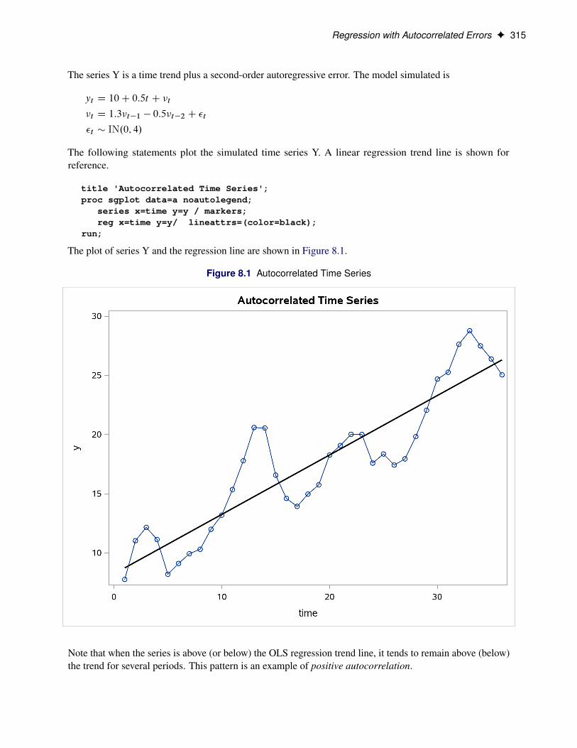
The series Y is a time trend plus a second-order autoregressive error. The model simulated is
yt D 10C 0:5t C �t
�t D 1:3�t�1 � 0:5�t�2 C �t
�t � IN.0; 4/
The following statements plot the simulated time series Y. A linear regression trend line is shown forreference.
title 'Autocorrelated Time Series';proc sgplot data=a noautolegend;
series x=time y=y / markers;reg x=time y=y/ lineattrs=(color=black);
run;
The plot of series Y and the regression line are shown in Figure 8.1.
Figure 8.1 Autocorrelated Time Series
Note that when the series is above (or below) the OLS regression trend line, it tends to remain above (below)the trend for several periods. This pattern is an example of positive autocorrelation.
316 F Chapter 8: The AUTOREG Procedure
Time series regression usually involves independent variables other than a time trend. However, the simpletime trend model is convenient for illustrating regression with autocorrelated errors, and the series Y shownin Figure 8.1 is used in the following introductory examples.
Ordinary Least Squares Regression
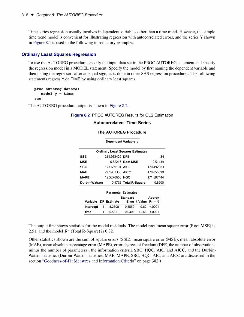
To use the AUTOREG procedure, specify the input data set in the PROC AUTOREG statement and specifythe regression model in a MODEL statement. Specify the model by first naming the dependent variable andthen listing the regressors after an equal sign, as is done in other SAS regression procedures. The followingstatements regress Y on TIME by using ordinary least squares:
proc autoreg data=a;model y = time;
run;
The AUTOREG procedure output is shown in Figure 8.2.
Figure 8.2 PROC AUTOREG Results for OLS Estimation
Autocorrelated Time Series
The AUTOREG Procedure
Dependent Variable y
Ordinary Least Squares Estimates
SSE 214.953429 DFE 34
MSE 6.32216 Root MSE 2.51439
SBC 173.659101 AIC 170.492063
MAE 2.01903356 AICC 170.855699
MAPE 12.5270666 HQC 171.597444
Durbin-Watson 0.4752 Total R-Square 0.8200
Parameter Estimates
Variable DF EstimateStandard
Error t ValueApproxPr > |t|
Intercept 1 8.2308 0.8559 9.62 <.0001
time 1 0.5021 0.0403 12.45 <.0001
The output first shows statistics for the model residuals. The model root mean square error (Root MSE) is2.51, and the model R2 (Total R-Square) is 0.82.
Other statistics shown are the sum of square errors (SSE), mean square error (MSE), mean absolute error(MAE), mean absolute percentage error (MAPE), error degrees of freedom (DFE, the number of observationsminus the number of parameters), the information criteria SBC, HQC, AIC, and AICC, and the Durbin-Watson statistic. (Durbin-Watson statistics, MAE, MAPE, SBC, HQC, AIC, and AICC are discussed in thesection “Goodness-of-Fit Measures and Information Criteria” on page 382.)

Regression with Autocorrelated Errors F 317
The output then shows a table of regression coefficients, with standard errors and t tests. The estimated modelis
yt D 8:23C 0:502t C �t
Est. Var.�t / D 6:32
The OLS parameter estimates are reasonably close to the true values, but the estimated error variance, 6.32,is much larger than the true value, 4.
Autoregressive Error Model
The following statements regress Y on TIME with the errors assumed to follow a second-order autoregressiveprocess. The order of the autoregressive model is specified by the NLAG=2 option. The Yule-Walkerestimation method is used by default. The example uses the METHOD=ML option to specify the exactmaximum likelihood method instead.
ods graphics on;proc autoreg data=a;
model y = time / nlag=2 method=ml;run;
The first part of the results is shown in Figure 8.3. The initial OLS results are produced first, followed byestimates of the autocorrelations computed from the OLS residuals. The autocorrelations are also displayedgraphically.
Figure 8.3 Preliminary Estimate for AR(2) Error Model
Autocorrelated Time Series
The AUTOREG Procedure
Dependent Variable y
Ordinary Least Squares Estimates
SSE 214.953429 DFE 34
MSE 6.32216 Root MSE 2.51439
SBC 173.659101 AIC 170.492063
MAE 2.01903356 AICC 170.855699
MAPE 12.5270666 HQC 171.597444
Durbin-Watson 0.4752 Total R-Square 0.8200
Parameter Estimates
Variable DF EstimateStandard
Error t ValueApproxPr > |t|
Intercept 1 8.2308 0.8559 9.62 <.0001
time 1 0.5021 0.0403 12.45 <.0001
Preliminary MSE 1.7943

318 F Chapter 8: The AUTOREG Procedure
Figure 8.4 Estimates of Autocorrelations
The maximum likelihood estimates are shown in Figure 8.5. This figure also shows the preliminary Yule-Walker estimates that are used as starting values for the iterative computation of the maximum likelihoodestimates.
Figure 8.5 Maximum Likelihood Estimates of AR(2) Error Model
Estimates of AutoregressiveParameters
Lag CoefficientStandard
Error t Value
1 -1.169057 0.148172 -7.89
2 0.545379 0.148172 3.68
Algorithm converged.
Maximum Likelihood Estimates
SSE 54.7493022 DFE 32
MSE 1.71092 Root MSE 1.30802
SBC 133.476508 AIC 127.142432
MAE 0.98307236 AICC 128.432755
MAPE 6.45517689 HQC 129.353194
Log Likelihood -59.571216 Transformed Regression R-Square 0.7280
Durbin-Watson 2.2761 Total R-Square 0.9542
Observations 36
Parameter Estimates
Variable DF EstimateStandard
Error t ValueApproxPr > |t|
Intercept 1 7.8833 1.1693 6.74 <.0001
time 1 0.5096 0.0551 9.25 <.0001
AR1 1 -1.2464 0.1385 -9.00 <.0001
AR2 1 0.6283 0.1366 4.60 <.0001
Autoregressive parameters assumed given
Variable DF EstimateStandard
Error t ValueApproxPr > |t|
Intercept 1 7.8833 1.1678 6.75 <.0001
time 1 0.5096 0.0551 9.26 <.0001
Regression with Autocorrelated Errors F 319
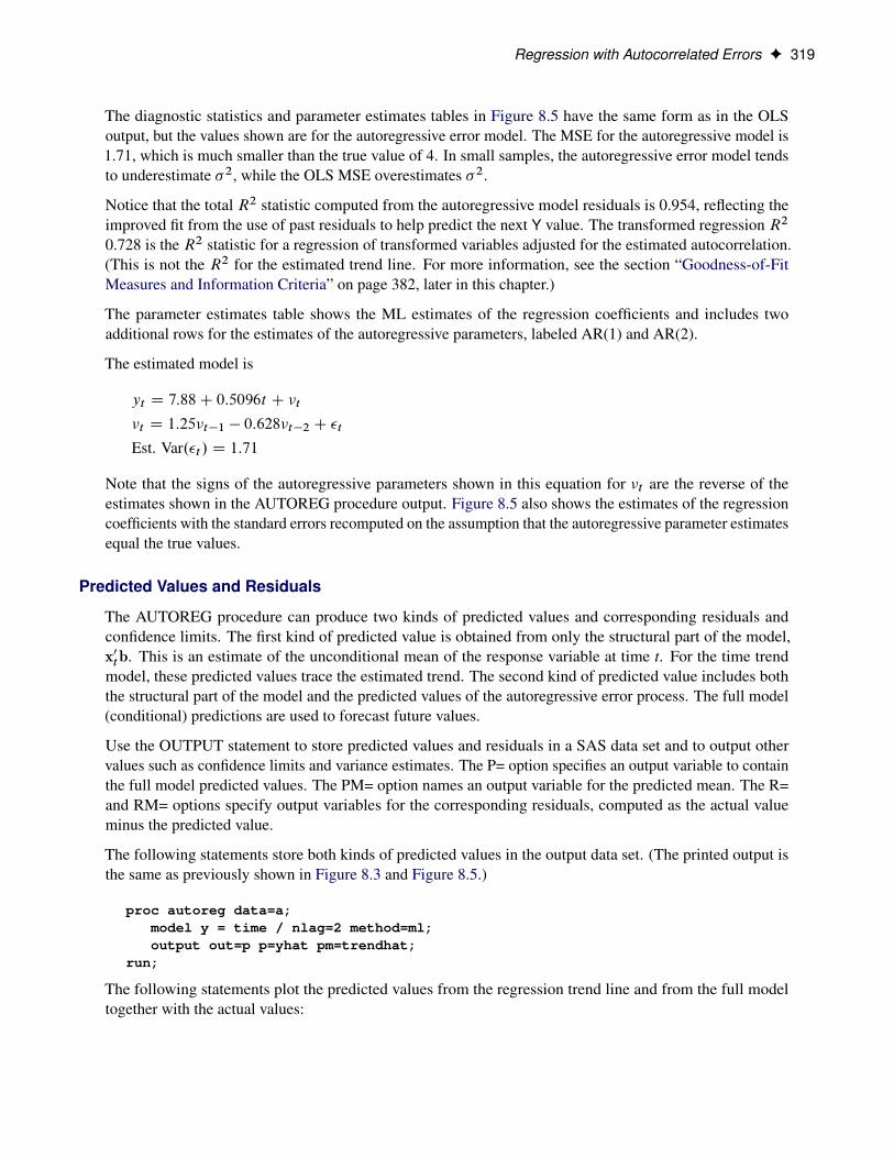
The diagnostic statistics and parameter estimates tables in Figure 8.5 have the same form as in the OLSoutput, but the values shown are for the autoregressive error model. The MSE for the autoregressive model is1.71, which is much smaller than the true value of 4. In small samples, the autoregressive error model tendsto underestimate �2, while the OLS MSE overestimates �2.
Notice that the total R2 statistic computed from the autoregressive model residuals is 0.954, reflecting theimproved fit from the use of past residuals to help predict the next Y value. The transformed regression R2
0.728 is the R2 statistic for a regression of transformed variables adjusted for the estimated autocorrelation.(This is not the R2 for the estimated trend line. For more information, see the section “Goodness-of-FitMeasures and Information Criteria” on page 382, later in this chapter.)
The parameter estimates table shows the ML estimates of the regression coefficients and includes twoadditional rows for the estimates of the autoregressive parameters, labeled AR(1) and AR(2).
The estimated model is
yt D 7:88C 0:5096t C �t
�t D 1:25�t�1 � 0:628�t�2 C �t
Est. Var.�t / D 1:71
Note that the signs of the autoregressive parameters shown in this equation for �t are the reverse of theestimates shown in the AUTOREG procedure output. Figure 8.5 also shows the estimates of the regressioncoefficients with the standard errors recomputed on the assumption that the autoregressive parameter estimatesequal the true values.
Predicted Values and Residuals
The AUTOREG procedure can produce two kinds of predicted values and corresponding residuals andconfidence limits. The first kind of predicted value is obtained from only the structural part of the model,x0tb. This is an estimate of the unconditional mean of the response variable at time t. For the time trendmodel, these predicted values trace the estimated trend. The second kind of predicted value includes boththe structural part of the model and the predicted values of the autoregressive error process. The full model(conditional) predictions are used to forecast future values.
Use the OUTPUT statement to store predicted values and residuals in a SAS data set and to output othervalues such as confidence limits and variance estimates. The P= option specifies an output variable to containthe full model predicted values. The PM= option names an output variable for the predicted mean. The R=and RM= options specify output variables for the corresponding residuals, computed as the actual valueminus the predicted value.
The following statements store both kinds of predicted values in the output data set. (The printed output isthe same as previously shown in Figure 8.3 and Figure 8.5.)
proc autoreg data=a;model y = time / nlag=2 method=ml;output out=p p=yhat pm=trendhat;
run;
The following statements plot the predicted values from the regression trend line and from the full modeltogether with the actual values:
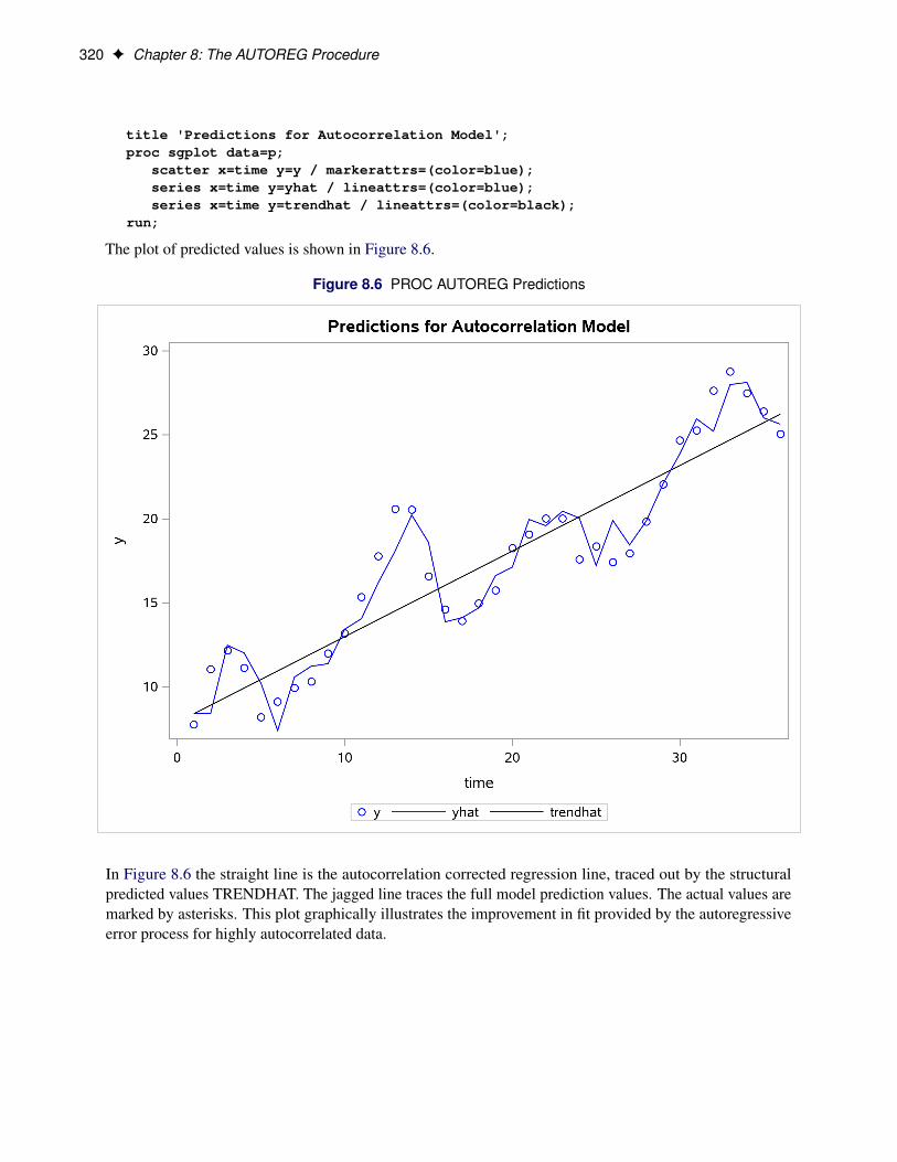
320 F Chapter 8: The AUTOREG Procedure
title 'Predictions for Autocorrelation Model';proc sgplot data=p;
scatter x=time y=y / markerattrs=(color=blue);series x=time y=yhat / lineattrs=(color=blue);series x=time y=trendhat / lineattrs=(color=black);
run;
The plot of predicted values is shown in Figure 8.6.
Figure 8.6 PROC AUTOREG Predictions
In Figure 8.6 the straight line is the autocorrelation corrected regression line, traced out by the structuralpredicted values TRENDHAT. The jagged line traces the full model prediction values. The actual values aremarked by asterisks. This plot graphically illustrates the improvement in fit provided by the autoregressiveerror process for highly autocorrelated data.
Forecasting Autoregressive Error Models F 321
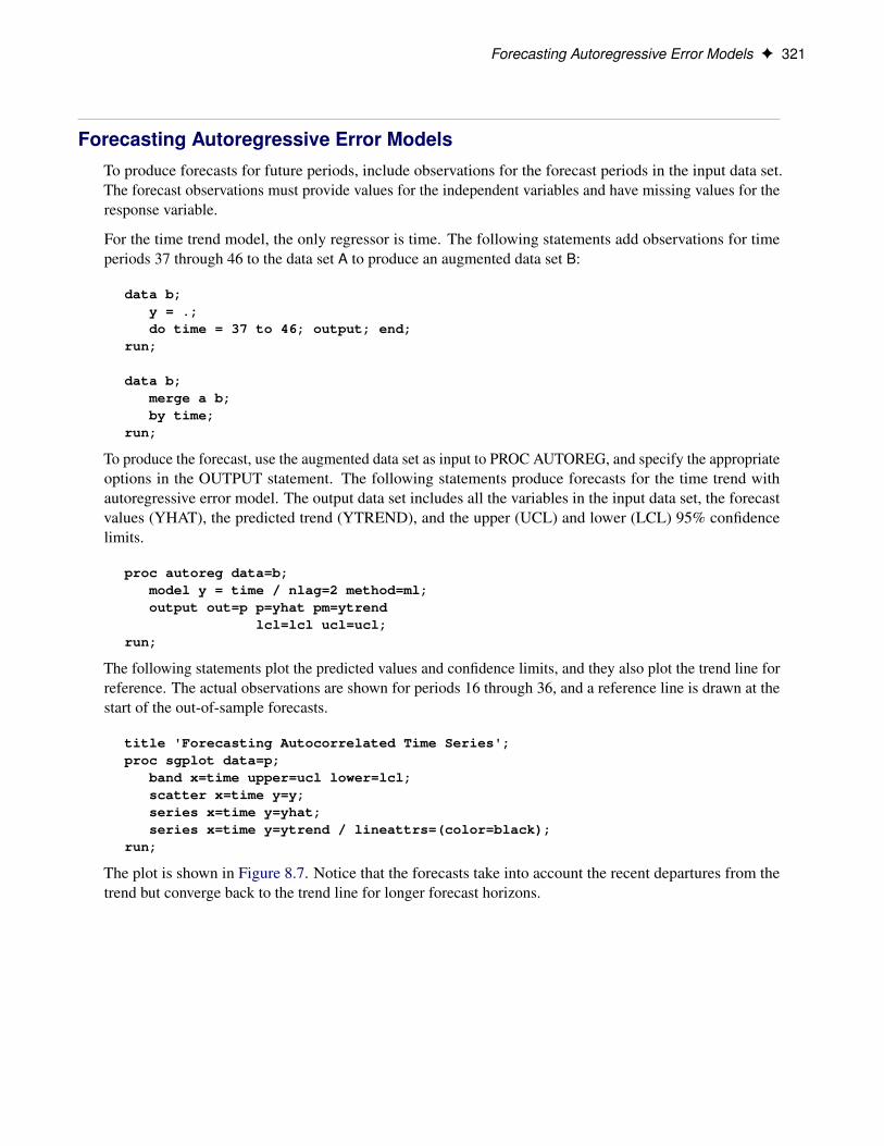
Forecasting Autoregressive Error ModelsTo produce forecasts for future periods, include observations for the forecast periods in the input data set.The forecast observations must provide values for the independent variables and have missing values for theresponse variable.
For the time trend model, the only regressor is time. The following statements add observations for timeperiods 37 through 46 to the data set A to produce an augmented data set B:
data b;y = .;do time = 37 to 46; output; end;
run;
data b;merge a b;by time;
run;
To produce the forecast, use the augmented data set as input to PROC AUTOREG, and specify the appropriateoptions in the OUTPUT statement. The following statements produce forecasts for the time trend withautoregressive error model. The output data set includes all the variables in the input data set, the forecastvalues (YHAT), the predicted trend (YTREND), and the upper (UCL) and lower (LCL) 95% confidencelimits.
proc autoreg data=b;model y = time / nlag=2 method=ml;output out=p p=yhat pm=ytrend
lcl=lcl ucl=ucl;run;
The following statements plot the predicted values and confidence limits, and they also plot the trend line forreference. The actual observations are shown for periods 16 through 36, and a reference line is drawn at thestart of the out-of-sample forecasts.
title 'Forecasting Autocorrelated Time Series';proc sgplot data=p;
band x=time upper=ucl lower=lcl;scatter x=time y=y;series x=time y=yhat;series x=time y=ytrend / lineattrs=(color=black);
run;
The plot is shown in Figure 8.7. Notice that the forecasts take into account the recent departures from thetrend but converge back to the trend line for longer forecast horizons.
322 F Chapter 8: The AUTOREG Procedure
Figure 8.7 PROC AUTOREG Forecasts
Testing for AutocorrelationIn the preceding section, it is assumed that the order of the autoregressive process is known. In practice, youneed to test for the presence of autocorrelation.
The Durbin-Watson test is a widely used method of testing for autocorrelation. The first-order Durbin-Watson statistic is printed by default. This statistic can be used to test for first-order autocorrelation. Usethe DWPROB option to print the significance level (p-values) for the Durbin-Watson tests. (Since theDurbin-Watson p-values are computationally expensive, they are not reported by default.)
You can use the DW= option to request higher-order Durbin-Watson statistics. Since the ordinary Durbin-Watson statistic tests only for first-order autocorrelation, the Durbin-Watson statistics for higher-orderautocorrelation are called generalized Durbin-Watson statistics.
The following statements perform the Durbin-Watson test for autocorrelation in the OLS residuals for orders1 through 4. The DWPROB option prints the marginal significance levels (p-values) for the Durbin-Watsonstatistics.

Testing for Autocorrelation F 323
/*-- Durbin-Watson test for autocorrelation --*/proc autoreg data=a;
model y = time / dw=4 dwprob;run;
The AUTOREG procedure output is shown in Figure 8.8. In this case, the first-order Durbin-Watson test ishighly significant, with p < .0001 for the hypothesis of no first-order autocorrelation. Thus, autocorrelationcorrection is needed.
Figure 8.8 Durbin-Watson Test Results for OLS Residuals
Forecasting Autocorrelated Time Series
The AUTOREG Procedure
Dependent Variable y
Ordinary Least Squares Estimates
SSE 214.953429 DFE 34
MSE 6.32216 Root MSE 2.51439
SBC 173.659101 AIC 170.492063
MAE 2.01903356 AICC 170.855699
MAPE 12.5270666 HQC 171.597444
Total R-Square 0.8200
Durbin-Watson Statistics
Order DW Pr < DW Pr > DW
1 0.4752 <.0001 1.0000
2 1.2935 0.0137 0.9863
3 2.0694 0.6545 0.3455
4 2.5544 0.9818 0.0182
NOTE: Pr<DW is the p-value for testing positive autocorrelation, and Pr>DW is the p-value fortesting negative autocorrelation.
Parameter Estimates
Variable DF EstimateStandard
Error t ValueApproxPr > |t|
Intercept 1 8.2308 0.8559 9.62 <.0001
time 1 0.5021 0.0403 12.45 <.0001
Using the Durbin-Watson test, you can decide if autocorrelation correction is needed. However, generalizedDurbin-Watson tests should not be used to decide on the autoregressive order. The higher-order testsassume the absence of lower-order autocorrelation. If the ordinary Durbin-Watson test indicates no first-order autocorrelation, you can use the second-order test to check for second-order autocorrelation. Onceautocorrelation is detected, further tests at higher orders are not appropriate. In Figure 8.8, since the first-orderDurbin-Watson test is significant, the order 2, 3, and 4 tests can be ignored.
When using Durbin-Watson tests to check for autocorrelation, you should specify an order at least as largeas the order of any potential seasonality, since seasonality produces autocorrelation at the seasonal lag. Forexample, for quarterly data use DW=4, and for monthly data use DW=12.
324 F Chapter 8: The AUTOREG Procedure
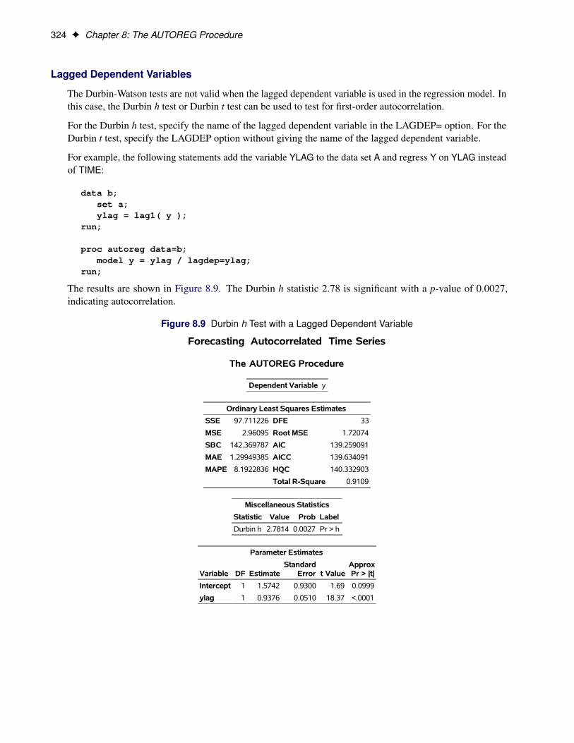
Lagged Dependent Variables
The Durbin-Watson tests are not valid when the lagged dependent variable is used in the regression model. Inthis case, the Durbin h test or Durbin t test can be used to test for first-order autocorrelation.
For the Durbin h test, specify the name of the lagged dependent variable in the LAGDEP= option. For theDurbin t test, specify the LAGDEP option without giving the name of the lagged dependent variable.
For example, the following statements add the variable YLAG to the data set A and regress Y on YLAG insteadof TIME:
data b;set a;ylag = lag1( y );
run;
proc autoreg data=b;model y = ylag / lagdep=ylag;
run;
The results are shown in Figure 8.9. The Durbin h statistic 2.78 is significant with a p-value of 0.0027,indicating autocorrelation.
Figure 8.9 Durbin h Test with a Lagged Dependent Variable
Forecasting Autocorrelated Time Series
The AUTOREG Procedure
Dependent Variable y
Ordinary Least Squares Estimates
SSE 97.711226 DFE 33
MSE 2.96095 Root MSE 1.72074
SBC 142.369787 AIC 139.259091
MAE 1.29949385 AICC 139.634091
MAPE 8.1922836 HQC 140.332903
Total R-Square 0.9109
Miscellaneous Statistics
Statistic Value Prob Label
Durbin h 2.7814 0.0027 Pr > h
Parameter Estimates
Variable DF EstimateStandard
Error t ValueApproxPr > |t|
Intercept 1 1.5742 0.9300 1.69 0.0999
ylag 1 0.9376 0.0510 18.37 <.0001

Stepwise Autoregression F 325
Stepwise AutoregressionOnce you determine that autocorrelation correction is needed, you must select the order of the autoregressiveerror model to use. One way to select the order of the autoregressive error model is stepwise autoregression.The stepwise autoregression method initially fits a high-order model with many autoregressive lags and thensequentially removes autoregressive parameters until all remaining autoregressive parameters have significantt tests.
To use stepwise autoregression, specify the BACKSTEP option, and specify a large order with the NLAG=option. The following statements show the stepwise feature, using an initial order of 5:
/*-- stepwise autoregression --*/proc autoreg data=a;
model y = time / method=ml nlag=5 backstep;run;
The results are shown in Figure 8.10.
Figure 8.10 Stepwise Autoregression
Forecasting Autocorrelated Time Series
The AUTOREG Procedure
Dependent Variable y
Ordinary Least Squares Estimates
SSE 214.953429 DFE 34
MSE 6.32216 Root MSE 2.51439
SBC 173.659101 AIC 170.492063
MAE 2.01903356 AICC 170.855699
MAPE 12.5270666 HQC 171.597444
Durbin-Watson 0.4752 Total R-Square 0.8200
Parameter Estimates
Variable DF EstimateStandard
Error t ValueApproxPr > |t|
Intercept 1 8.2308 0.8559 9.62 <.0001
time 1 0.5021 0.0403 12.45 <.0001
Backward Elimination ofAutoregressive Terms
Lag Estimate t Value Pr > |t|
4 -0.052908 -0.20 0.8442
3 0.115986 0.57 0.5698
5 0.131734 1.21 0.2340
326 F Chapter 8: The AUTOREG Procedure
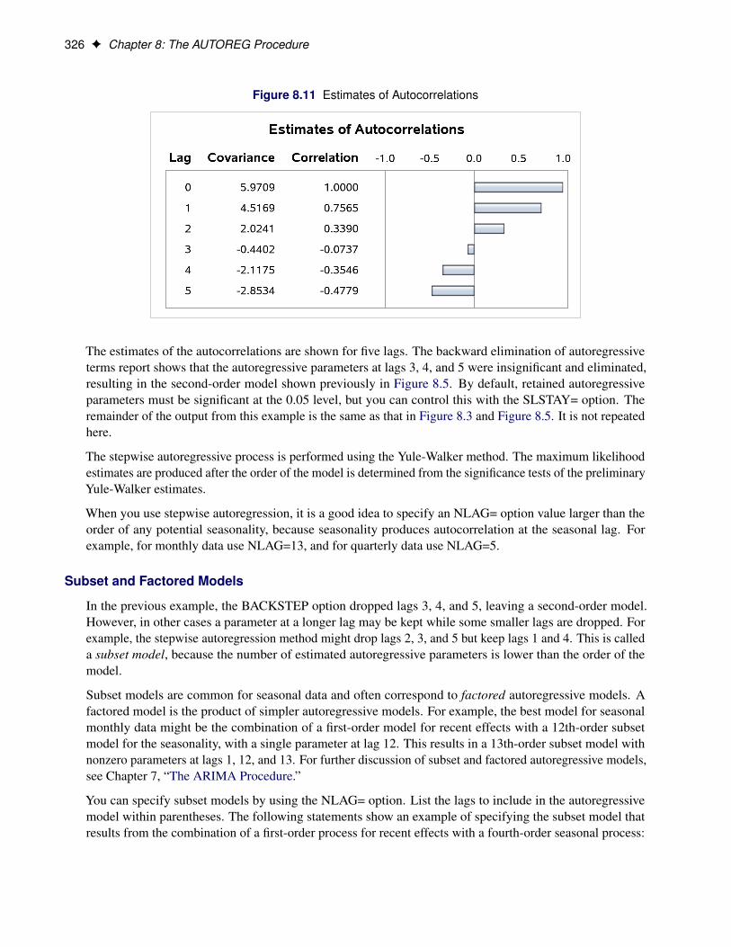
Figure 8.11 Estimates of Autocorrelations
The estimates of the autocorrelations are shown for five lags. The backward elimination of autoregressiveterms report shows that the autoregressive parameters at lags 3, 4, and 5 were insignificant and eliminated,resulting in the second-order model shown previously in Figure 8.5. By default, retained autoregressiveparameters must be significant at the 0.05 level, but you can control this with the SLSTAY= option. Theremainder of the output from this example is the same as that in Figure 8.3 and Figure 8.5. It is not repeatedhere.
The stepwise autoregressive process is performed using the Yule-Walker method. The maximum likelihoodestimates are produced after the order of the model is determined from the significance tests of the preliminaryYule-Walker estimates.
When you use stepwise autoregression, it is a good idea to specify an NLAG= option value larger than theorder of any potential seasonality, because seasonality produces autocorrelation at the seasonal lag. Forexample, for monthly data use NLAG=13, and for quarterly data use NLAG=5.
Subset and Factored Models
In the previous example, the BACKSTEP option dropped lags 3, 4, and 5, leaving a second-order model.However, in other cases a parameter at a longer lag may be kept while some smaller lags are dropped. Forexample, the stepwise autoregression method might drop lags 2, 3, and 5 but keep lags 1 and 4. This is calleda subset model, because the number of estimated autoregressive parameters is lower than the order of themodel.
Subset models are common for seasonal data and often correspond to factored autoregressive models. Afactored model is the product of simpler autoregressive models. For example, the best model for seasonalmonthly data might be the combination of a first-order model for recent effects with a 12th-order subsetmodel for the seasonality, with a single parameter at lag 12. This results in a 13th-order subset model withnonzero parameters at lags 1, 12, and 13. For further discussion of subset and factored autoregressive models,see Chapter 7, “The ARIMA Procedure.”
You can specify subset models by using the NLAG= option. List the lags to include in the autoregressivemodel within parentheses. The following statements show an example of specifying the subset model thatresults from the combination of a first-order process for recent effects with a fourth-order seasonal process:
Testing for Heteroscedasticity F 327
/*-- specifying the lags --*/proc autoreg data=a;
model y = time / nlag=(1 4 5);run;
The MODEL statement specifies the following fifth-order autoregressive error model:
yt D aC bt C �t
�t D �'1�t�1 � '4�t�4 � '5�t�5 C �t
Testing for HeteroscedasticityOne of the key assumptions of the ordinary regression model is that the errors have the same variancethroughout the sample. This is also called the homoscedasticity model. If the error variance is not constant,the data are said to be heteroscedastic.
Since ordinary least squares regression assumes constant error variance, heteroscedasticity causes the OLSestimates to be inefficient. Models that take into account the changing variance can make more efficientuse of the data. Also, heteroscedasticity can make the OLS forecast error variance inaccurate because thepredicted forecast variance is based on the average variance instead of on the variability at the end of theseries.
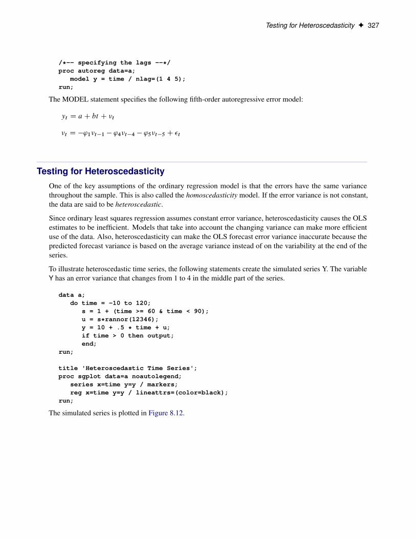
To illustrate heteroscedastic time series, the following statements create the simulated series Y. The variableY has an error variance that changes from 1 to 4 in the middle part of the series.
data a;do time = -10 to 120;
s = 1 + (time >= 60 & time < 90);u = s*rannor(12346);y = 10 + .5 * time + u;if time > 0 then output;end;
run;
title 'Heteroscedastic Time Series';proc sgplot data=a noautolegend;
series x=time y=y / markers;reg x=time y=y / lineattrs=(color=black);
run;
The simulated series is plotted in Figure 8.12.
328 F Chapter 8: The AUTOREG Procedure
Figure 8.12 Heteroscedastic and Autocorrelated Series
To test for heteroscedasticity with PROC AUTOREG, specify the ARCHTEST option. The followingstatements regress Y on TIME and use the ARCHTEST= option to test for heteroscedastic OLS residuals:
/*-- test for heteroscedastic OLS residuals --*/proc autoreg data=a;
model y = time / archtest;output out=r r=yresid;
run;
The PROC AUTOREG output is shown in Figure 8.13. The Q statistics test for changes in variance acrosstime by using lag windows that range from 1 through 12. (For more information, see the section “Testing forNonlinear Dependence: Heteroscedasticity Tests” on page 403.) The p-values for the test statistics stronglyindicate heteroscedasticity, with p < 0.0001 for all lag windows.

Testing for Heteroscedasticity F 329
The Lagrange multiplier (LM) tests also indicate heteroscedasticity. These tests can also help determine theorder of the ARCH model that is appropriate for modeling the heteroscedasticity, assuming that the changingvariance follows an autoregressive conditional heteroscedasticity model.
Figure 8.13 Heteroscedasticity Tests
Heteroscedastic Time Series
The AUTOREG Procedure
Dependent Variable y
Ordinary Least Squares Estimates
SSE 223.645647 DFE 118
MSE 1.89530 Root MSE 1.37670
SBC 424.828766 AIC 419.253783
MAE 0.97683599 AICC 419.356347
MAPE 2.73888672 HQC 421.517809
Durbin-Watson 2.4444 Total R-Square 0.9938
Tests for ARCH Disturbances Based onOLS Residuals
Order Q Pr > Q LM Pr > LM
1 19.4549 <.0001 19.1493 <.0001
2 21.3563 <.0001 19.3057 <.0001
3 28.7738 <.0001 25.7313 <.0001
4 38.1132 <.0001 26.9664 <.0001
5 52.3745 <.0001 32.5714 <.0001
6 54.4968 <.0001 34.2375 <.0001
7 55.3127 <.0001 34.4726 <.0001
8 58.3809 <.0001 34.4850 <.0001
9 68.3075 <.0001 38.7244 <.0001
10 73.2949 <.0001 38.9814 <.0001
11 74.9273 <.0001 39.9395 <.0001
12 76.0254 <.0001 40.8144 <.0001
Parameter Estimates
Variable DF EstimateStandard
Error t ValueApproxPr > |t|
Intercept 1 9.8684 0.2529 39.02 <.0001
time 1 0.5000 0.003628 137.82 <.0001
The tests of Lee and King (1993) and Wong and Li (1995) can also be applied to check the absence of ARCHeffects. The following example shows that Wong and Li’s test is robust to detect the presence of ARCHeffects with the existence of outliers:

330 F Chapter 8: The AUTOREG Procedure
/*-- data with outliers at observation 10 --*/data b;
do time = -10 to 120;s = 1 + (time >= 60 & time < 90);u = s*rannor(12346);y = 10 + .5 * time + u;if time = 10 then
do; y = 200; end;if time > 0 then output;
end;run;/*-- test for heteroscedastic OLS residuals --*/proc autoreg data=b;
model y = time / archtest=(qlm) ;model y = time / archtest=(lk,wl) ;
run;
As shown in Figure 8.14, the p-values of Q or LM statistics for all lag windows are above 90%, which failsto reject the null hypothesis of the absence of ARCH effects. Lee and King’s test, which rejects the nullhypothesis for lags more than 8 at 10% significance level, works better. Wong and Li’s test works best,rejecting the null hypothesis and detecting the presence of ARCH effects for all lag windows.
Figure 8.14 Heteroscedasticity Tests
Heteroscedastic Time Series
The AUTOREG Procedure
Tests for ARCH Disturbances Basedon OLS Residuals
Order Q Pr > Q LM Pr > LM
1 0.0076 0.9304 0.0073 0.9319
2 0.0150 0.9925 0.0143 0.9929
3 0.0229 0.9991 0.0217 0.9992
4 0.0308 0.9999 0.0290 0.9999
5 0.0367 1.0000 0.0345 1.0000
6 0.0442 1.0000 0.0413 1.0000
7 0.0522 1.0000 0.0485 1.0000
8 0.0612 1.0000 0.0565 1.0000
9 0.0701 1.0000 0.0643 1.0000
10 0.0701 1.0000 0.0742 1.0000
11 0.0701 1.0000 0.0838 1.0000
12 0.0702 1.0000 0.0939 1.0000

Heteroscedasticity and GARCH Models F 331
Figure 8.14 continued
Tests for ARCH Disturbances Based onOLS Residuals
Order LK Pr > |LK| WL Pr > WL
1 -0.6377 0.5236 34.9984 <.0001
2 -0.8926 0.3721 72.9542 <.0001
3 -1.0979 0.2723 104.0322 <.0001
4 -1.2705 0.2039 139.9328 <.0001
5 -1.3824 0.1668 176.9830 <.0001
6 -1.5125 0.1304 200.3388 <.0001
7 -1.6385 0.1013 238.4844 <.0001
8 -1.7695 0.0768 267.8882 <.0001
9 -1.8881 0.0590 304.5706 <.0001
10 -2.2349 0.0254 326.3658 <.0001
11 -2.2380 0.0252 348.8036 <.0001
12 -2.2442 0.0248 371.9596 <.0001
Heteroscedasticity and GARCH ModelsThere are several approaches to dealing with heteroscedasticity. If the error variance at different times isknown, weighted regression is a good method. If, as is usually the case, the error variance is unknown andmust be estimated from the data, you can model the changing error variance.
The generalized autoregressive conditional heteroscedasticity (GARCH) model is one approach to modelingtime series with heteroscedastic errors. The GARCH regression model with autoregressive errors is
yt D x0tˇ C �t
�t D �t � '1�t�1 � � � � � 'm�t�m
�t Dphtet
ht D ! C
qXiD1
˛i�2t�i C
pXjD1
jht�j
et � IN.0; 1/
This model combines the mth-order autoregressive error model with the GARCH.p; q/ variance model. It isdenoted as the AR.m/-GARCH.p; q/ regression model.
The tests for the presence of ARCH effects (namely, Q and LM tests, tests from Lee and King (1993) andtests from Wong and Li (1995)) can help determine the order of the ARCH model appropriate for the data.For example, the Lagrange multiplier (LM) tests shown in Figure 8.13 are significant .p < 0:0001/ throughorder 12, which indicates that a very high-order ARCH model is needed to model the heteroscedasticity.
The basic ARCH.q/model .p D 0/ is a short memory process in that only the most recent q squared residualsare used to estimate the changing variance. The GARCH model .p > 0/ allows long memory processes,which use all the past squared residuals to estimate the current variance. The LM tests in Figure 8.13 suggestthe use of the GARCH model .p > 0/ instead of the ARCH model.
332 F Chapter 8: The AUTOREG Procedure
The GARCH.p; q/ model is specified with the GARCH=(P=p, Q=q) option in the MODEL statement. Thebasic ARCH.q/ model is the same as the GARCH.0; q/ model and is specified with the GARCH=(Q=q)option.
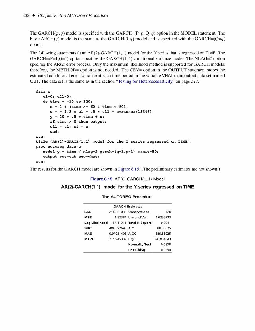
The following statements fit an AR(2)-GARCH.1; 1/ model for the Y series that is regressed on TIME. TheGARCH=(P=1,Q=1) option specifies the GARCH.1; 1/ conditional variance model. The NLAG=2 optionspecifies the AR(2) error process. Only the maximum likelihood method is supported for GARCH models;therefore, the METHOD= option is not needed. The CEV= option in the OUTPUT statement stores theestimated conditional error variance at each time period in the variable VHAT in an output data set namedOUT. The data set is the same as in the section “Testing for Heteroscedasticity” on page 327.
data c;ul=0; ull=0;do time = -10 to 120;
s = 1 + (time >= 60 & time < 90);u = + 1.3 * ul - .5 * ull + s*rannor(12346);y = 10 + .5 * time + u;if time > 0 then output;ull = ul; ul = u;end;
run;title 'AR(2)-GARCH(1,1) model for the Y series regressed on TIME';proc autoreg data=c;
model y = time / nlag=2 garch=(q=1,p=1) maxit=50;output out=out cev=vhat;
run;
The results for the GARCH model are shown in Figure 8.15. (The preliminary estimates are not shown.)
Figure 8.15 AR(2)-GARCH.1; 1/ Model
AR(2)-GARCH(1,1) model for the Y series regressed on TIME
The AUTOREG Procedure
GARCH Estimates
SSE 218.861036 Observations 120
MSE 1.82384 Uncond Var 1.6299733
Log Likelihood -187.44013 Total R-Square 0.9941
SBC 408.392693 AIC 388.88025
MAE 0.97051406 AICC 389.88025
MAPE 2.75945337 HQC 396.804343
Normality Test 0.0838
Pr > ChiSq 0.9590

Heteroscedasticity and GARCH Models F 333
Figure 8.15 continued
Parameter Estimates
Variable DF EstimateStandard
Error t ValueApproxPr > |t|
Intercept 1 8.9301 0.7456 11.98 <.0001
time 1 0.5075 0.0111 45.90 <.0001
AR1 1 -1.2301 0.1111 -11.07 <.0001
AR2 1 0.5023 0.1090 4.61 <.0001
ARCH0 1 0.0850 0.0780 1.09 0.2758
ARCH1 1 0.2103 0.0873 2.41 0.0159
GARCH1 1 0.7375 0.0989 7.46 <.0001
The normality test is not significant (p = 0.959), which is consistent with the hypothesis that the residualsfrom the GARCH model, �t=
pht , are normally distributed. The parameter estimates table includes rows for
the GARCH parameters. ARCH0 represents the estimate for the parameter !, ARCH1 represents ˛1, andGARCH1 represents 1.
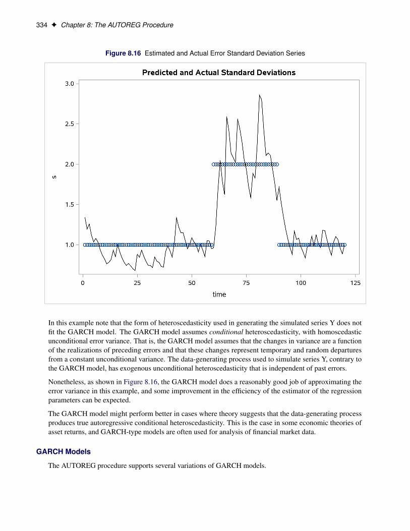
The following statements transform the estimated conditional error variance series VHAT to the estimatedstandard deviation series SHAT. Then, they plot SHAT together with the true standard deviation S used togenerate the simulated data.
data out;set out;shat = sqrt( vhat );
run;
title 'Predicted and Actual Standard Deviations';proc sgplot data=out noautolegend;
scatter x=time y=s;series x=time y=shat/ lineattrs=(color=black);
run;
The plot is shown in Figure 8.16.
334 F Chapter 8: The AUTOREG Procedure
Figure 8.16 Estimated and Actual Error Standard Deviation Series
In this example note that the form of heteroscedasticity used in generating the simulated series Y does notfit the GARCH model. The GARCH model assumes conditional heteroscedasticity, with homoscedasticunconditional error variance. That is, the GARCH model assumes that the changes in variance are a functionof the realizations of preceding errors and that these changes represent temporary and random departuresfrom a constant unconditional variance. The data-generating process used to simulate series Y, contrary tothe GARCH model, has exogenous unconditional heteroscedasticity that is independent of past errors.
Nonetheless, as shown in Figure 8.16, the GARCH model does a reasonably good job of approximating theerror variance in this example, and some improvement in the efficiency of the estimator of the regressionparameters can be expected.
The GARCH model might perform better in cases where theory suggests that the data-generating processproduces true autoregressive conditional heteroscedasticity. This is the case in some economic theories ofasset returns, and GARCH-type models are often used for analysis of financial market data.
GARCH Models
The AUTOREG procedure supports several variations of GARCH models.

Syntax: AUTOREG Procedure F 335
Using the TYPE= option along with the GARCH= option enables you to control the constraints placedon the estimated GARCH parameters. You can specify unconstrained, nonnegativity-constrained (default),stationarity-constrained, or integration-constrained models. The integration constraint produces the integratedGARCH (IGARCH) model.
You can also use the TYPE= option to specify the exponential form of the GARCH model, called theEGARCH model, or other types of GARCH models, namely the quadratic GARCH (QGARCH), thresholdGARCH (TGARCH), and power GARCH (PGARCH) models. The MEAN= option along with the GARCH=option specifies the GARCH-in-mean (GARCH-M) model.
The following statements illustrate the use of the TYPE= option to fit an AR(2)-EGARCH.1; 1/ model to theseries Y. (Output is not shown.)
/*-- AR(2)-EGARCH(1,1) model --*/proc autoreg data=a;
model y = time / nlag=2 garch=(p=1,q=1,type=exp);run;
For more information, see the section “GARCH Models” on page 373.
Syntax: AUTOREG ProcedureThe AUTOREG procedure is controlled by the following statements:
PROC AUTOREG options ;BY variables ;CLASS variables ;MODEL dependent = regressors / options ;HETERO variables / options ;NLOPTIONS options ;OUTPUT < OUT=SAS-data-set > < options > < keyword=name > ;RESTRICT equation , . . . , equation ;TEST equation , . . . , equation / option ;
At least one MODEL statement must be specified. One OUTPUT statement can follow each MODELstatement. One HETERO statement can follow each MODEL statement.
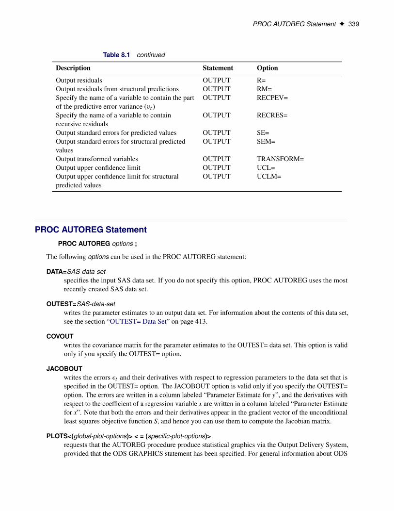
Functional SummaryThe statements and options used with the AUTOREG procedure are summarized in Table 8.1.
Table 8.1 AUTOREG Functional Summary
Description Statement Option
Data Set OptionsSpecify the input data set AUTOREG DATA=Write parameter estimates to an output data set AUTOREG OUTEST=

336 F Chapter 8: The AUTOREG Procedure
Table 8.1 continued
Description Statement Option
Include covariances in the OUTEST= data set AUTOREG COVOUTInclude errors and their derivatives in theOUTEST= data set
AUTOREG JACOBOUT
Request that the procedure produce graphics viathe Output Delivery System
AUTOREG PLOTS=
Write predictions, residuals, and confidence limitsto an output data set
OUTPUT OUT=
Declaring the Role of VariablesSpecify BY-group processing BYSpecify classification variables CLASS
Printing Control OptionsRequest all printing options MODEL ALLPrint transformed coefficients MODEL COEFPrint correlation matrix of the estimates MODEL CORRBPrint covariance matrix of the estimates MODEL COVBPrint DW statistics up to order j MODEL DW=jPrint marginal probability of the generalizedDurbin-Watson test statistics for large samplesizes
MODEL DWPROB
Print the p-values for the Durbin-Watson test becomputed using a linearized approximation of thedesign matrix
MODEL LDW
Print inverse of Toeplitz matrix MODEL GINVPrint the Godfrey LM serial correlation test MODEL GODFREY=Print details at each iteration step MODEL ITPRINTPrint the Durbin t statistic MODEL LAGDEPPrint the Durbin h statistic MODEL LAGDEP=Print the log-likelihood value of the regressionmodel
MODEL LOGLIKL
Print the Jarque-Bera normality test MODEL NORMALPrint the tests for the absence of ARCH effects MODEL ARCHTEST=Print BDS tests for independence MODEL BDS=Print rank version of von Neumann ratio test forindependence
MODEL VNRRANK=
Print runs test for independence MODEL RUNS=Print the turning point test for independence MODEL TP=Print the Lagrange multiplier test HETERO TEST=LMPrint Bai-Perron tests for multiple structuralchanges
MODEL BP=
Print the Chow test for structural change MODEL CHOW=Print the predictive Chow test for structuralchange
MODEL PCHOW=

Functional Summary F 337
Table 8.1 continued
Description Statement Option
Suppress printed output MODEL NOPRINTPrint partial autocorrelations MODEL PARTIALPrint Ramsey’s RESET test MODEL RESETPrint augmented Dickey-Fuller tests forstationarity or unit roots
MODEL STATIONARITY=(ADF=)
Print ERS tests for stationarity or unit roots MODEL STATIONARITY=(ERS=)Print KPSS tests or Shin tests for stationarity orcointegration
MODEL STATIONARITY=(KPSS=)
Print Ng-Perron tests for stationarity or unit roots MODEL STATIONARITY=(NP=)Print Phillips-Perron tests for stationarity or unitroots
MODEL STATIONARITY=(PHILLIPS=)
Print tests of linear hypotheses TESTSpecify the test statistics to use TEST TYPE=Print the uncentered regression R2 MODEL URSQ
Options to Control the Optimization ProcessSpecify the optimization options NLOPTIONS See Chapter 6, “Nonlinear
Optimization Methods.”
Model Estimation OptionsSpecify the order of autoregressive process MODEL NLAG=Center the dependent variable MODEL CENTERSuppress the intercept parameter MODEL NOINTRemove nonsignificant AR parameters MODEL BACKSTEPSpecify significance level for BACKSTEP MODEL SLSTAY=Specify the convergence criterion MODEL CONVERGE=Specify the type of covariance matrix MODEL COVEST=Set the initial values of parameters used by theiterative optimization algorithm
MODEL INITIAL=
Specify iterative Yule-Walker method MODEL ITERSpecify maximum number of iterations MODEL MAXITER=Specify the estimation method MODEL METHOD=Use only first sequence of nonmissing data MODEL NOMISSSpecify the optimization technique MODEL OPTMETHOD=Imposes restrictions on the regression estimates RESTRICTEstimate and test heteroscedasticity models HETERO
GARCH Related OptionsSpecify order of GARCH process MODEL GARCH=(Q=,P=)Specify type of GARCH model MODEL GARCH=(. . . ,TYPE=)Specify various forms of the GARCH-M model MODEL GARCH=(. . . ,MEAN=)Suppress GARCH intercept parameter MODEL GARCH=(. . . ,NOINT)Specify the trust region method MODEL GARCH=(. . . ,TR)Estimate the GARCH model for the conditional tdistribution
MODEL GARCH=(. . . ) DIST=

338 F Chapter 8: The AUTOREG Procedure
Table 8.1 continued
Description Statement Option
Estimate the start-up values for the conditionalvariance equation
MODEL GARCH=(. . . ,STARTUP=)
Specify the functional form of theheteroscedasticity model
HETERO LINK=
Specify that the heteroscedasticity model does notinclude the unit term
HETERO NOCONST
Impose constraints on the estimated parameters inthe heteroscedasticity model
HETERO COEF=
Impose constraints on the estimated standarddeviation of the heteroscedasticity model
HETERO STD=
Output conditional error variance OUTPUT CEV=Output conditional prediction error variance OUTPUT CPEV=Specify the flexible conditional variance form ofthe GARCH model
HETERO
Output Control OptionsSpecify confidence limit size OUTPUT ALPHACLI=Specify confidence limit size for structuralpredicted values
OUTPUT ALPHACLM=
Specify the significance level for the upper andlower bounds of the CUSUM and CUSUMSQstatistics
OUTPUT ALPHACSM=
Specify the name of a variable to contain thevalues of the Theil’s BLUS residuals
OUTPUT BLUS=
Output the value of the error variance �2t OUTPUT CEV=Output transformed intercept variable OUTPUT CONSTANT=Specify the name of a variable to contain theCUSUM statistics
OUTPUT CUSUM=
Specify the name of a variable to contain theCUSUMSQ statistics
OUTPUT CUSUMSQ=
Specify the name of a variable to contain theupper confidence bound for the CUSUM statistic
OUTPUT CUSUMUB=
Specify the name of a variable to contain thelower confidence bound for the CUSUM statistic
OUTPUT CUSUMLB=
Specify the name of a variable to contain theupper confidence bound for the CUSUMSQstatistic
OUTPUT CUSUMSQUB=
Specify the name of a variable to contain the lowerconfidence bound for the CUSUMSQ statistic
OUTPUT CUSUMSQLB=
Output lower confidence limit OUTPUT LCL=Output lower confidence limit for structuralpredicted values
OUTPUT LCLM=
Output predicted values OUTPUT P=Output predicted values of structural part OUTPUT PM=
PROC AUTOREG Statement F 339
Table 8.1 continued
Description Statement Option
Output residuals OUTPUT R=Output residuals from structural predictions OUTPUT RM=Specify the name of a variable to contain the partof the predictive error variance (vt )
OUTPUT RECPEV=
Specify the name of a variable to containrecursive residuals
OUTPUT RECRES=
Output standard errors for predicted values OUTPUT SE=Output standard errors for structural predictedvalues
OUTPUT SEM=
Output transformed variables OUTPUT TRANSFORM=Output upper confidence limit OUTPUT UCL=Output upper confidence limit for structuralpredicted values
OUTPUT UCLM=
PROC AUTOREG StatementPROC AUTOREG options ;
The following options can be used in the PROC AUTOREG statement:
DATA=SAS-data-setspecifies the input SAS data set. If you do not specify this option, PROC AUTOREG uses the mostrecently created SAS data set.
OUTEST=SAS-data-setwrites the parameter estimates to an output data set. For information about the contents of this data set,see the section “OUTEST= Data Set” on page 413.
COVOUTwrites the covariance matrix for the parameter estimates to the OUTEST= data set. This option is validonly if you specify the OUTEST= option.
JACOBOUTwrites the errors �t and their derivatives with respect to regression parameters to the data set that isspecified in the OUTEST= option. The JACOBOUT option is valid only if you specify the OUTEST=option. The errors are written in a column labeled “Parameter Estimate for y”, and the derivatives withrespect to the coefficient of a regression variable x are written in a column labeled “Parameter Estimatefor x”. Note that both the errors and their derivatives appear in the gradient vector of the unconditionalleast squares objective function S, and hence you can use them to compute the Jacobian matrix.
PLOTS<(global-plot-options)> < = (specific-plot-options)>requests that the AUTOREG procedure produce statistical graphics via the Output Delivery System,provided that the ODS GRAPHICS statement has been specified. For general information about ODS

340 F Chapter 8: The AUTOREG Procedure
Graphics, see Chapter 21, “Statistical Graphics Using ODS” (SAS/STAT User’s Guide). The global-plot-options apply to all relevant plots generated by the AUTOREG procedure. The global-plot-optionssupported by the AUTOREG procedure follow.
Global Plot Options
ONLY suppresses the default plots. Only the plots specifically requested are produced.
UNPACKPANEL | UNPACK displays each graph separately. (By default, some graphs can appeartogether in a single panel.)
Specific Plot Options
ALL requests that all plots appropriate for the particular analysis be produced.
ACF produces the autocorrelation function plot.
IACF produces the inverse autocorrelation function plot of residuals.
PACF produces the partial autocorrelation function plot of residuals.
FITPLOT plots the predicted and actual values.
COOKSD produces the Cook’s D plot.
QQ Q-Q plot of residuals.
RESIDUAL | RES plots the residuals.
STUDENTRESIDUAL plots the studentized residuals. For the models with the NLAG= or GARCH=options in the MODEL statement or with the HETERO statement, this option isreplaced by the STANDARDRESIDUAL option.
STANDARDRESIDUAL plots the standardized residuals.
WHITENOISE plots the white noise probabilities.
RESIDUALHISTOGRAM | RESIDHISTOGRAM plots the histogram of residuals.
NONE suppresses all plots.
In addition, any of the following MODEL statement options can be specified in the PROC AUTOREGstatement, which is equivalent to specifying the option for every MODEL statement: ALL, ARCHTEST,BACKSTEP, CENTER, COEF, CONVERGE=, CORRB, COVB, DW=, DWPROB, GINV, ITER, ITPRINT,MAXITER=, METHOD=, NOINT, NOMISS, NOPRINT, and PARTIAL.
BY StatementBY variables ;
A BY statement can be used with PROC AUTOREG to obtain separate analyses on observations in groupsdefined by the BY variables.

CLASS Statement F 341
CLASS StatementCLASS variables ;
The CLASS statement names the classification variables to be used in the analysis. Classification variablescan be either character or numeric.
In PROC AUTOREG, the CLASS statement enables you to output classification variables to a data set thatcontains a copy of the original data.
Class levels are determined from the formatted values of the CLASS variables. Thus, you can use formatsto group values into levels. For more information, see the discussion of the FORMAT procedure in SASLanguage Reference: Dictionary.
MODEL StatementMODEL dependent = regressors / options ;
The MODEL statement specifies the dependent variable and independent regressor variables for the regressionmodel. If no independent variables are specified in the MODEL statement, only the mean is fitted. (This is away to obtain autocorrelations of a series.)
Models can be given labels of up to eight characters. Model labels are used in the printed output to identifythe results for different models. The model label is specified as follows:
label : MODEL . . . ;
The following options can be used in the MODEL statement after a slash (/).
CENTERcenters the dependent variable by subtracting its mean and suppresses the intercept parameter from themodel. This option is valid only when the model does not have regressors (explanatory variables).
NOINTsuppresses the intercept parameter.
Autoregressive Error Options
NLAG=number
NLAG=(number-list)specifies the order of the autoregressive error process or the subset of autoregressive error lags to befitted. Note that NLAG=3 is the same as NLAG=(1 2 3). If the NLAG= option is not specified, PROCAUTOREG does not fit an autoregressive model.
GARCH Estimation Options
DIST=valuespecifies the distribution assumed for the error term in GARCH-type estimation. If no GARCH=option is specified, the option is ignored. If EGARCH is specified, the distribution is always the normaldistribution. The values of the DIST= option are as follows:
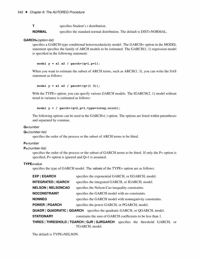
342 F Chapter 8: The AUTOREG Procedure
T specifies Student’s t distribution.
NORMAL specifies the standard normal distribution. The default is DIST=NORMAL.
GARCH=(option-list)specifies a GARCH-type conditional heteroscedasticity model. The GARCH= option in the MODELstatement specifies the family of ARCH models to be estimated. The GARCH.1; 1/ regression modelis specified in the following statement:
model y = x1 x2 / garch=(q=1,p=1);
When you want to estimate the subset of ARCH terms, such as ARCH.1; 3/, you can write the SASstatement as follows:
model y = x1 x2 / garch=(q=(1 3));
With the TYPE= option, you can specify various GARCH models. The IGARCH.2; 1/ model withouttrend in variance is estimated as follows:
model y = / garch=(q=2,p=1,type=integ,noint);
The following options can be used in the GARCH=( ) option. The options are listed within parenthesesand separated by commas.
Q=numberQ=(number-list)
specifies the order of the process or the subset of ARCH terms to be fitted.
P=numberP=(number-list)
specifies the order of the process or the subset of GARCH terms to be fitted. If only the P= option isspecified, P= option is ignored and Q=1 is assumed.
TYPE=valuespecifies the type of GARCH model. The values of the TYPE= option are as follows:
EXP | EGARCH specifies the exponential GARCH, or EGARCH, model.
INTEGRATED | IGARCH specifies the integrated GARCH, or IGARCH, model.
NELSON | NELSONCAO specifies the Nelson-Cao inequality constraints.
NOCONSTRAINT specifies the GARCH model with no constraints.
NONNEG specifies the GARCH model with nonnegativity constraints.
POWER | PGARCH specifies the power GARCH, or PGARCH, model.
QUADR | QUADRATIC | QGARCH specifies the quadratic GARCH, or QGARCH, model.
STATIONARY constrains the sum of GARCH coefficients to be less than 1.
THRES | THRESHOLD | TGARCH | GJR | GJRGARCH specifies the threshold GARCH, orTGARCH, model.
The default is TYPE=NELSON.

MODEL Statement F 343
MEAN=valuespecifies the functional form of the GARCH-M model. You can specify the following values:
LINEAR specifies the linear function:
yt D x0tˇ C ıht C �t
LOG specifies the log function:
yt D x0tˇ C ı ln.ht /C �t
SQRT specifies the square root function:
yt D x0tˇ C ıpht C �t
NOINTsuppresses the intercept parameter in the conditional variance model. This option is valid only whenyou also specify the TYPE=INTEG option.
STARTUP=MSE | ESTIMATErequests that the positive constant c for the start-up values of the GARCH conditional error varianceprocess be estimated. By default, or if you specify STARTUP=MSE, the value of the mean squarederror is used as the default constant.
TRuses the trust region method for GARCH estimation. This algorithm is numerically stable, althoughcomputation is expensive. The double quasi-Newton method is the default.
Printing Options
ALLrequests all printing options.
ARCHTEST
ARCHTEST=(option-list)specifies tests for the absence of ARCH effects. The following options can be used in theARCHTEST=( ) option. The options are listed within parentheses and separated by commas.
QLM | QLMARCH requests the Q and Engle’s LM tests.
LK | LKARCH requests Lee and King’s ARCH tests.
WL | WLARCH requests Wong and Li’s ARCH tests.
ALL requests all ARCH tests, namely Q and Engle’s LM tests, Lee and King’s tests,and Wong and Li’s tests.
If ARCHTEST is defined without additional suboptions, it requests the Q and Engle’s LM tests. Thatis, the statement
344 F Chapter 8: The AUTOREG Procedure
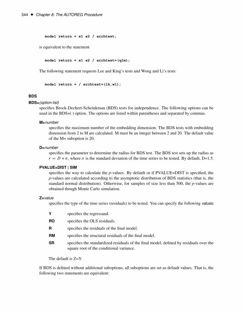
model return = x1 x2 / archtest;
is equivalent to the statement
model return = x1 x2 / archtest=(qlm);
The following statement requests Lee and King’s tests and Wong and Li’s tests:
model return = / archtest=(lk,wl);
BDS
BDS=(option-list)specifies Brock-Dechert-Scheinkman (BDS) tests for independence. The following options can beused in the BDS=( ) option. The options are listed within parentheses and separated by commas.
M=numberspecifies the maximum number of the embedding dimension. The BDS tests with embeddingdimension from 2 to M are calculated. M must be an integer between 2 and 20. The default valueof the M= suboption is 20.
D=numberspecifies the parameter to determine the radius for BDS test. The BDS test sets up the radius asr D D � � , where � is the standard deviation of the time series to be tested. By default, D=1.5.
PVALUE=DIST | SIMspecifies the way to calculate the p-values. By default or if PVALUE=DIST is specified, thep-values are calculated according to the asymptotic distribution of BDS statistics (that is, thestandard normal distribution). Otherwise, for samples of size less than 500, the p-values areobtained though Monte Carlo simulation.
Z=valuespecifies the type of the time series (residuals) to be tested. You can specify the following values:
Y specifies the regressand.
RO specifies the OLS residuals.
R specifies the residuals of the final model.
RM specifies the structural residuals of the final model.
SR specifies the standardized residuals of the final model, defined by residuals over thesquare root of the conditional variance.
The default is Z=Y.
If BDS is defined without additional suboptions, all suboptions are set as default values. That is, thefollowing two statements are equivalent:

MODEL Statement F 345
model return = x1 x2 / nlag=1 BDS;
model return = x1 x2 / nlag=1 BDS=(M=20, D=1.5, PVALUE=DIST, Z=Y);
To do the specification check of a GARCH(1,1) model, you can write the SAS statement as follows:
model return = / garch=(p=1,q=1) BDS=(Z=SR);
BP
BP=(option-list)specifies Bai-Perron (BP) tests for multiple structural changes, introduced in Bai and Perron (1998).You can specify the following options in parentheses and separated by commas.
EPS=numberspecifies the minimum length of regime; that is, if EPS=", then for any i; i D 1; : : : ;M ,Ti � Ti�1 � T", where T is the sample size; M is the number of breaks specified in the M=option; .T1 : : : TM / are the break dates; and T0 D 0 and TMC1 D T . The restriction that.M C 1/" � 1 is required. By default, EPS=0.05.
ETA=numberspecifies that the second method is to be used in the calculation of the supF.l C 1jl/ test, andthe minimum length of regime for the new additional break date is .Ti � Ti�1/� if ETA=� andthe new break date is in regime i for the given break dates .T1 : : : Tl/. The default value of theETA= suboption is the missing value; that is, the first method is to be used in the calculationof the supF.l C 1jl/ test and, no matter which regime the new break date is in, the minimumlength of regime for the new additional break date is T" when EPS=".
HAC<(option-list)>specifies that the heteroscedasticity- and autocorrelation-consistent estimator be applied in theestimation of the variance covariance matrix and the confidence intervals of break dates. Whenyou specify this option, you can specify the following options within parentheses and separatedby commas:
KERNEL=valuespecifies the type of kernel function. You can specify the following values:
BARTLETT specifies the Bartlett kernel function.
PARZEN specifies the Parzen kernel function.
QUADRATICSPECTRAL | QS specifies the quadratic spectral kernel function.
TRUNCATED specifies the truncated kernel function.
TUKEYHANNING | TUKEY | TH specifies the Tukey-Hanning kernel function.
By default, KERNEL=QUADRATICSPECTRAL.
346 F Chapter 8: The AUTOREG Procedure
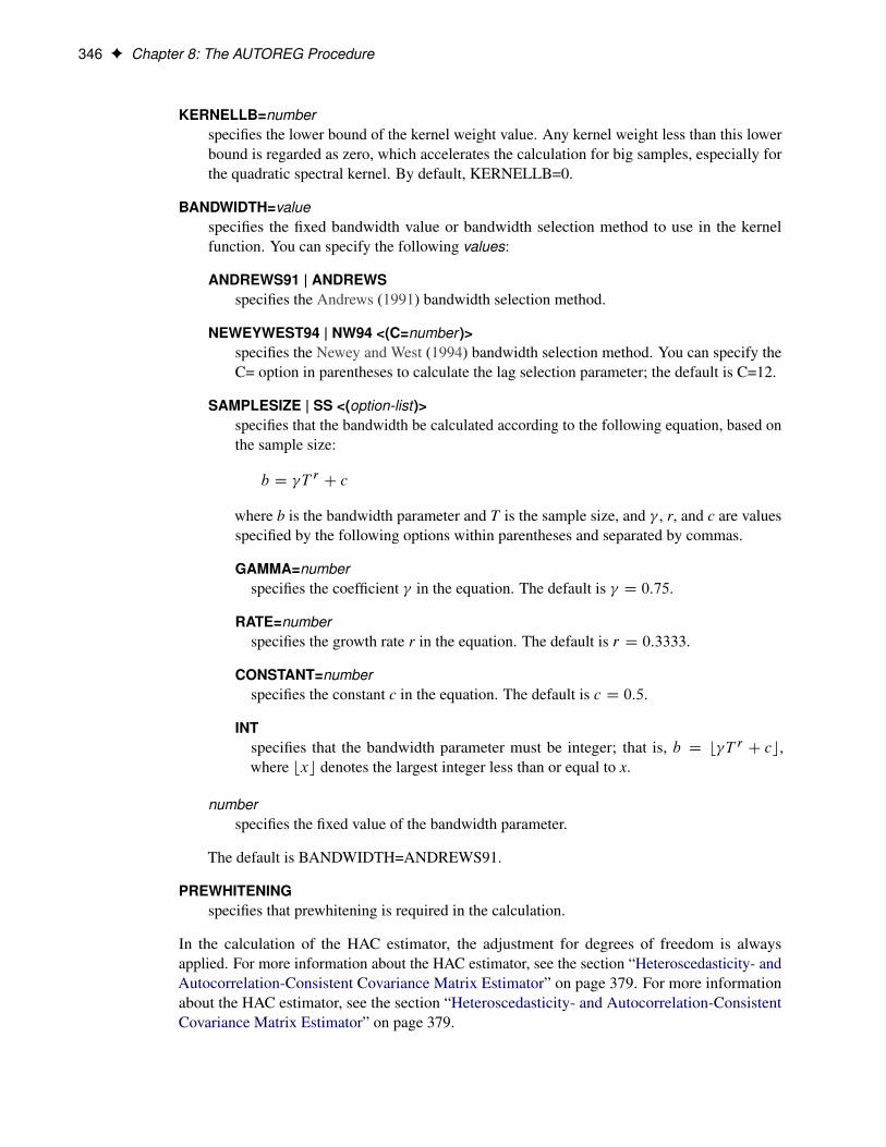
KERNELLB=numberspecifies the lower bound of the kernel weight value. Any kernel weight less than this lowerbound is regarded as zero, which accelerates the calculation for big samples, especially forthe quadratic spectral kernel. By default, KERNELLB=0.
BANDWIDTH=valuespecifies the fixed bandwidth value or bandwidth selection method to use in the kernelfunction. You can specify the following values:
ANDREWS91 | ANDREWSspecifies the Andrews (1991) bandwidth selection method.
NEWEYWEST94 | NW94 <(C=number )>specifies the Newey and West (1994) bandwidth selection method. You can specify theC= option in parentheses to calculate the lag selection parameter; the default is C=12.
SAMPLESIZE | SS <(option-list)>specifies that the bandwidth be calculated according to the following equation, based onthe sample size:
b D T r C c
where b is the bandwidth parameter and T is the sample size, and , r, and c are valuesspecified by the following options within parentheses and separated by commas.
GAMMA=numberspecifies the coefficient in the equation. The default is D 0:75.
RATE=numberspecifies the growth rate r in the equation. The default is r D 0:3333.
CONSTANT=numberspecifies the constant c in the equation. The default is c D 0:5.
INTspecifies that the bandwidth parameter must be integer; that is, b D b T r C cc,where bxc denotes the largest integer less than or equal to x.
numberspecifies the fixed value of the bandwidth parameter.
The default is BANDWIDTH=ANDREWS91.
PREWHITENINGspecifies that prewhitening is required in the calculation.
In the calculation of the HAC estimator, the adjustment for degrees of freedom is alwaysapplied. For more information about the HAC estimator, see the section “Heteroscedasticity- andAutocorrelation-Consistent Covariance Matrix Estimator” on page 379. For more informationabout the HAC estimator, see the section “Heteroscedasticity- and Autocorrelation-ConsistentCovariance Matrix Estimator” on page 379.

MODEL Statement F 347
HEspecifies that the errors are assumed to have heterogeneous distribution across regimes in theestimation of covariance matrix.
HOspecifies that �is in the calculation of confidence intervals of break dates are different acrossregimes.
HQspecifies that Qis in the calculation of confidence intervals of break dates are different acrossregimes.
HRspecifies that the regressors are assumed to have heterogeneous distribution across regimes in theestimation of covariance matrix.
M=numberspecifies the number of breaks. For a given M, the following tests are to be performed: (1) thesupF tests of no break versus the alternative hypothesis that there are i breaks, i D 1; : : : ;M ;(2) the UDmaxF and WDmaxF double maximum tests of no break versus the alternativehypothesis that there are unknown number of breaks up to M; and (3) the supF.l C 1jl/ tests ofl versus l C 1 breaks, l D 0; : : : ;M . The restriction that .M C 1/" � 1 is required, where " isspecified in the EPS= option. By default, M=5.
NTHREADS=numberspecifies the number of threads to be used for parallel computing. The default is the number ofCPUs available.
P=numberspecifies the number of covariates whose coefficients are unchanged over time in the partialstructural change model. The first P=p independent variables that are specified in the MODELstatement have unchanged coefficients; the rest of the independent variables have coefficients thatchange across regimes. The default is P=0; that is, the pure structural change model is estimated.
PRINTEST=ALL | BIC | LWZ | NONE | SEQ<(number)> | numberspecifies in which structural change models the parameter estimates are to be printed. You canspecify the following option values:
ALL specifies that the parameter estimates in all structural change models with m breaks,m D 0; : : : ;M , be printed.
BIC specifies that the parameter estimates in the structural change model that minimizesthe BIC information criterion be printed.
LWZ specifies that the parameter estimates in the structural change model that minimizesthe LWZ information criterion be printed.
NONE specifies that none of the parameter estimates be printed.
SEQ specifies that the parameter estimates in the structural change model that is chosen bysequentially applying supF.lC1jl/ tests, l from 0 to M, be printed. If you specify theSEQ option, you can also specify the significance level in the parentheses, for example,SEQ(0.10). The first l such that the p-value of supF.l C 1jl/ test is greater than the
348 F Chapter 8: The AUTOREG Procedure
significance level is selected as the number of breaks in the structural change model.By default, the significance level 5% is used for the SEQ option; that is, specifyingSEQ is equivalent to specifying SEQ(0.05).
number specifies that the parameter estimates in the structural change model with the specifiednumber of breaks be printed. If the specified number is greater than the numberspecified in the M= option, none of the parameter estimates are printed; that is, it isequivalent to specifying the NONE option.
The default is PRINTEST=ALL.
If you define the BP option without additional suboptions, all suboptions are set as default values. Thatis, the following two statements are equivalent:
model y = z1 z2 / BP;
model y = z1 z2 / BP=(M=5, P=0, EPS=0.05, PRINTEST=ALL);
To apply the HAC estimator with the Bartlett kernel function and print only the parameter estimatesin the structural change model selected by the LWZ information criterion, you can write the SASstatement as follows:
model y = z1 z2 / BP=(HAC(KERNEL=BARTLETT), PRINTEST=LWZ);
To specify a partial structural change model, you can write the SAS statement as follows:
model y = x1 x2 x3 z1 z2 / NOINT BP=(P=3);
CHOW=( obs1 . . . obsn )computes Chow tests to evaluate the stability of the regression coefficient. The Chow test is also calledthe analysis-of-variance test.
Each value obsi listed on the CHOW= option specifies a break point of the sample. The sample isdivided into parts at the specified break point, with observations before obsi in the first part and obsiand later observations in the second part, and the fits of the model in the two parts are compared towhether both parts of the sample are consistent with the same model.
The break points obsi refer to observations within the time range of the dependent variable, ignoringmissing values before the start of the dependent series. Thus, CHOW=20 specifies the 20th observationafter the first nonmissing observation for the dependent variable. For example, if the dependent variableY contains 10 missing values before the first observation with a nonmissing Y value, then CHOW=20actually refers to the 30th observation in the data set.
When you specify the break point, you should note the number of presample missing values.

MODEL Statement F 349
COEFprints the transformation coefficients for the first p observations. These coefficients are formed from ascalar multiplied by the inverse of the Cholesky root of the Toeplitz matrix of autocovariances.
CORRBprints the estimated correlations of the parameter estimates.
COVBprints the estimated covariances of the parameter estimates.
COVEST=OP | HESSIAN | QML | HC0 | HC1 | HC2 | HC3 | HC4 | HAC <(. . . )> | NEWEYWEST <(. . . )>specifies the type of covariance matrix. You can specify the following values (by default,COVEST=OP):
OPuses the outer product matrix to compute the covariance matrix of the parameter estimates. Whenthe final model is an OLS or AR error model, this option is ignored; the method to calculatethe estimate of covariance matrix is illustrated in the section “Variance Estimates and StandardErrors” on page 371.
HESSIANproduces the covariance matrix by using the Hessian matrix. When the final model is an OLS orAR error model, this option is ignored; the method to calculate the estimate of covariance matrixis illustrated in the section “Variance Estimates and Standard Errors” on page 371.
QMLcomputes the quasi–maximum likelihood estimates. This option is equivalent to COVEST=HC0.When the final model is an OLS or AR error model, this option is ignored; the method to calculatethe estimate of covariance matrix is illustrated in the section “Variance Estimates and StandardErrors” on page 371.
HCncalculates the heteroscedasticity-consistent covariance matrix estimator (HCCME) that corre-sponds to n, where n = 0, 1, 2, 3, 4.
HAC<(options)>specifies the heteroscedasticity- and autocorrelation-consistent (HAC) covariance matrix esti-mator. When you specify this option, you can specify the following options in parentheses andseparate them with commas:
KERNEL=valuespecifies the type of kernel function. You can specify the following values:
BARTLETT specifies the Bartlett kernel function.
PARZEN specifies the Parzen kernel function.
QUADRATICSPECTRAL | QS specifies the quadratic spectral kernel function.
TRUNCATED specifies the truncated kernel function.
TUKEYHANNING | TUKEY | TH specifies the Tukey-Hanning kernel function.
By default, KERNEL=QUADRATICSPECTRAL.
350 F Chapter 8: The AUTOREG Procedure
KERNELLB=numberspecifies the lower bound of the kernel weight value. Any kernel weight less than numberis regarded as zero, which accelerates the calculation for big samples, especially for thequadratic spectral kernel. By default, KERNELLB=0.
BANDWIDTH=valuespecifies the fixed bandwidth value or bandwidth selection method to use in the kernelfunction. You can specify the following values:
ANDREWS91 | ANDREWS specifies the Andrews (1991) bandwidth selection method.
NEWEYWEST94 | NW94 <(C=number )> specifies the Newey and West (1994) band-width selection method. You can specify the C= option in the parenthesesto calculate the lag selection parameter; the default is C=12.
SAMPLESIZE | SS <(option-list)> calculates the bandwidth according to the followingequation, based on the sample size:
b D T r C c
where b is the bandwidth parameter; T is the sample size; and , r, andc are values specified by the following options within parentheses andseparated by commas.
GAMMA=numberspecifies the coefficient in the equation. The default is D 0:75.
RATE=numberspecifies the growth rate r in the equation. The default is r D 0:3333.
CONSTANT=numberspecifies the constant c in the equation. The default is c D 0:5.
INTspecifies that the bandwidth parameter must be integer; that is, b Db T r C cc, where bxc denotes the largest integer less than or equal tox.
number specifies the fixed value of the bandwidth parameter.
By default, BANDWIDTH=ANDREWS91.
PREWHITENINGspecifies that prewhitening is required in the calculation.
ADJUSTDFspecifies that the adjustment for degrees of freedom be required in the calculation.
NEWEYWEST<(options)>specifies the well-known Newey-West estimator, which is a special HAC estimator with (1) theBartlett kernel; (2) the bandwidth parameter determined by the equation based on the samplesize, b D b T r C cc; and (3) no adjustment for degrees of freedom and no prewhitening. Bydefault, the bandwidth parameter for the Newey-West estimator is
�0:75T 0:3333 C 0:5
˘, as
shown in equation (15.17) in Stock and Watson (2002). You can specify the following options inparentheses and separate them with commas:
MODEL Statement F 351
GAMMA=numberspecifies the coefficient in the equation. The default is D 0:75.
RATE=numberspecifies the growth rate r in the equation. The default is r D 0:3333.
CONSTANT=numberspecifies the constant c in the equation. The default is c D 0:5.
The following two statements are equivalent:
model y = x / COVEST=NEWEYWEST;
model y = x / COVEST=HAC(KERNEL=BARTLETT,BANDWIDTH=SAMPLESIZE(GAMMA=0.75,
RATE=0.3333,CONSTANT=0.5,INT));
Another popular sample-size-dependent bandwidth,jT 1=4 C 1:5
k, as mentioned in Newey and
West (1987), can be specified by the following statement:
model y = x / COVEST=NEWEYWEST(GAMMA=1,RATE=0.25,CONSTANT=1.5);
For more information about the HC0 to HC4, HAC, and Newey-West estimators, see the section“Heteroscedasticity- and Autocorrelation-Consistent Covariance Matrix Estimator” on page 379. Bydefault, COVEST=OP.
DW=nprints Durbin-Watson statistics up to the order n. When the LAGDEP option is specified, the Durbin-Watson statistic is not printed unless the DW= option is explicitly specified. By default, DW=1.
DWPROBnow produces p-values for the generalized Durbin-Watson test statistics for large sample sizes. Previ-ously, the Durbin-Watson probabilities were calculated only for small sample sizes. The new methodof calculating Durbin-Watson probabilities is based on the algorithm of Ansley, Kohn, and Shively(1992).
GINVprints the inverse of the Toeplitz matrix of autocovariances for the Yule-Walker solution. For moreinformation, see the section “Computational Methods” on page 370.
GODFREYGODFREY=r
produces Godfrey’s general Lagrange multiplier test against ARMA errors.
ITPRINTprints the objective function and parameter estimates at each iteration. The objective function is thefull log-likelihood function for the maximum likelihood method, while the error sum of squares isproduced as the objective function of unconditional least squares. For the ML method, the ITPRINToption prints the value of the full log-likelihood function, not the concentrated likelihood.

352 F Chapter 8: The AUTOREG Procedure
LAGDEP
LAGDVprints the Durbin t statistic, which is used to detect residual autocorrelation in the presence of laggeddependent variables. For more information, see the section “Generalized Durbin-Watson Tests” onpage 399.
LAGDEP=name
LAGDV=nameprints the Durbin h statistic for testing the presence of first-order autocorrelation when regressorscontain the lagged dependent variable whose name is specified as LAGDEP=name. If the Durbinh statistic cannot be computed, the asymptotically equivalent t statistic is printed instead. For moreinformation, see the section “Generalized Durbin-Watson Tests” on page 399.
When the regression model contains several lags of the dependent variable, specify the lagged dependentvariable for the smallest lag in the LAGDEP= option. For example:
model y = x1 x2 ylag2 ylag3 / lagdep=ylag2;
LOGLIKLprints the log-likelihood value of the regression model, assuming normally distributed errors.
NOPRINTsuppresses all printed output.
NORMALspecifies the Jarque-Bera’s normality test statistic for regression residuals.
PARTIALprints partial autocorrelations.
PCHOW=( obs1 . . . obsn )computes the predictive Chow test. The form of the PCHOW= option is the same as the form of theCHOW= option; see the discussion of the CHOW= option.
RESETproduces Ramsey’s RESET test statistics. The RESET option tests the null model
yt D xtˇ C ut
against the alternative
yt D xtˇ CpXjD2
�j Oyjt C ut
where Oyt is the predicted value from the OLS estimation of the null model. The RESET optionproduces three RESET test statistics for p D 2, 3, and 4.
MODEL Statement F 353
RUNS
RUNS=(Z=value)specifies the runs test for independence. The Z= suboption specifies the type of the time series orresiduals to be tested. The values of the Z= suboption are as follows:
Y specifies the regressand. The default is Z=Y.
RO specifies the OLS residuals.
R specifies the residuals of the final model.
RM specifies the structural residuals of the final model.
SR specifies the standardized residuals of the final model, defined by residuals over the squareroot of the conditional variance.
STATIONARITY=(test< =(test-options) > < , test< =(test-options) > > . . . < , test< =(test-options) > >)specifies tests of stationarity or unit roots. You can specify one of more of the following tests alongwith their test-options. For example, the following statement tests the stationarity of a variable byusing the augmented Dickey-Fuller unit root test and the KPSS test in which the quadratic spectralkernel is applied:
model y= / stationarity = (adf, kpss=(kernel=qs));
STATIONARITY=(ADF)
STATIONARITY=(ADF=(value . . . value)produces the augmented Dickey-Fuller unit root test (Dickey and Fuller 1979). As in thePhillips-Perron test, three regression models can be specified for the null hypothesis for theaugmented Dickey-Fuller test (zero mean, single mean, and trend). These models assume thatthe disturbances are distributed as white noise. The augmented Dickey-Fuller test can accountfor the serial correlation between the disturbances in some way. The model, with the time trendspecification for example, is
yt D �C �yt�1 C ıt C 1�yt�1 C � � � C p�yt�p C ut
This formulation has the advantage that it can accommodate higher-order autoregressive processesin ut . The test statistic follows the same distribution as the Dickey-Fuller test statistic. For moreinformation, see the section “PROBDF Function for Dickey-Fuller Tests” on page 157.
In the presence of regressors, the ADF option tests the cointegration relation between thedependent variable and the regressors. Following Engle and Granger (1987), a two-step estimationand testing procedure is carried out, in a fashion similar to the Phillips-Ouliaris test. The OLSresiduals of the regression in the MODEL statement are used to compute the t statistic of theaugmented Dickey-Fuller regression in a second step. Three cases arise based on which type ofdeterministic terms are included in the first step of regression. Only the constant term and lineartrend cases are practically useful (Davidson and MacKinnon 1993, page 721), and therefore arecomputed and reported. The test statistic, as shown in Phillips and Ouliaris (1990), follows thesame distribution as the OZt statistic in the Phillips-Ouliaris cointegration test. The asymptoticdistribution is tabulated in tables IIa–IIc of Phillips and Ouliaris (1990), and the finite sampledistribution is obtained in Table 2 and Table 3 in Engle and Yoo (1987) by Monte Carlo simulation.

354 F Chapter 8: The AUTOREG Procedure
STATIONARITY=(ERS)
STATIONARITY=(ERS=(value)
STATIONARITY=(NP)
STATIONARITY=(NP=(value)provides a class of efficient unit root tests, because they reduce the size distortion and improvethe power compared with traditional unit root tests such as the augmented Dickey-Fuller andPhillips-Perron tests. Two test statistics are reported with the ERS= suboption: the point optimaltest and the DF-GLS test, which are originally proposed in Elliott, Rothenberg, and Stock (1996).Elliott, Rothenberg, and Stock suggest using the Schwarz Bayesian information criterion to selectthe optimal lag length in the augmented Dickey-Fuller regression. The maximum lag length canbe specified by ERS=value. The minimum lag length is 3 and the default maximum lag length is8.
Six tests, namely MZ˛, MSB , MZt , the modified point optimal test, the point optimal test,and the DF-GLS test, which are discussed in Ng and Perron (2001), are reported with the NP=suboption. Ng and Perron suggest using the modified AIC to select the optimal lag length in theaugmented Dickey-Fuller regression by using GLS detrended data. The maximum lag length canbe specified by NP=value. The default maximum lag length is 8. The maximum lag length in theERS tests and Ng-Perron tests cannot exceed T=2 � 2, where T is the sample size.
STATIONARITY=(KPSS)
STATIONARITY=(KPSS=(KERNEL=(type))
STATIONARITY=(KPSS=(KERNEL=(type TRUNCPOINTMETHOD))produce the Kwiatkowski, Phillips, Schmidt, and Shin (1992) (KPSS) unit root test or Shin (1994)cointegration test.
Unlike the null hypothesis of the Dickey-Fuller and Phillips-Perron tests, the null hypothesis ofthe KPSS states that the time series is stationary. As a result, it tends to reject a random walkmore often. If the model does not have an intercept, the KPSS option performs the KPSS testfor three null hypothesis cases: zero mean, single mean, and deterministic trend. Otherwise, itreports the single mean and deterministic trend only. It computes a test statistic and providesp-value (Hobijn, Franses, and Ooms 2004) for the hypothesis that the random walk componentof the time series is equal to zero in the following cases (for more information, see the section“Kwiatkowski, Phillips, Schmidt, and Shin (KPSS) Unit Root Test and Shin Cointegration Test”on page 394):
Zero mean computes the KPSS test statistic based on the zero mean autoregressive model.
yt D ut
Single mean computes the KPSS test statistic based on the autoregressive model with aconstant term.
yt D �C ut
Trend computes the KPSS test statistic based on the autoregressive model withconstant and time trend terms.
yt D �C ıt C ut

MODEL Statement F 355
This test depends on the long-run variance of the series being defined as
�2T l D1
T
TXiD1
Ou2i C2
T
lXsD1
wsl
TXtDsC1
Out Out�s
where wsl is a kernel, s is a maximum lag (truncation point), and Out are OLS residuals or originaldata series. You can specify two types of the kernel:
KERNEL=NW | BART Newey-West (or Bartlett) kernel
w.s; l/ D 1 �s
l C 1
KERNEL=QS Quadratic spectral kernel
w.s=l/ D w.x/ D25
12�2x2
�sin .6�x=5/6�x=5
� cos .6�x=5/�
You can set the truncation point l by using three different methods:
SCHW=c Schwert maximum lag formula
l D max
(1;floor
"c
�T
100
�1=4#)
LAG=l LAG=l manually defined number of lags.
AUTO Automatic bandwidth selection (Hobijn, Franses, and Ooms 2004) (for moreinformation, see the section “Kwiatkowski, Phillips, Schmidt, and Shin(KPSS) Unit Root Test and Shin Cointegration Test” on page 394).
If STATIONARITY=KPSS is defined without additional parameters, the Newey-West kernel isused. For the Newey-West kernel the default is the Schwert truncation point method with c D 12.For the quadratic spectral kernel the default is AUTO.
The KPSS test can be used in general time series models because its limiting distribution isderived in the context of a class of weakly dependent and heterogeneously distributed data. Thelimiting probability for the KPSS test is computed assuming that error disturbances are normallydistributed. The p-values that are reported are based on the simulation of the limiting probabilityfor the KPSS test.
To test for stationarity of a variable, y, by using default KERNEL=NW and SCHW=12, you canuse the following statements:
/*-- test for stationarity of regression residuals --*/proc autoreg data=a;
model y= / stationarity = (KPSS);run;
To test for stationarity of a variable, y, by using quadratic spectral kernel and automatic bandwidthselection, you can use the following statements:
356 F Chapter 8: The AUTOREG Procedure
/*-- test for stationarity using quadraticspectral kernel and automatic bandwidth selection --*/
proc autoreg data=a;model y= /stationarity = (KPSS=(KERNEL=QS AUTO));
run;
If there are regressors in the MODEL statement except for the intercept, the Shin (1994) cointe-gration test, an extension of the KPSS test, is carried out. The limiting distribution of the tests,and then the reported p-values, are different from those in the KPSS tests. For more information,see the section “Kwiatkowski, Phillips, Schmidt, and Shin (KPSS) Unit Root Test and ShinCointegration Test” on page 394.
STATIONARITY=(PHILLIPS)
STATIONARITY=(PHILLIPS=(value . . . value)produces the Phillips-Perron unit root test when there are no regressors in the MODEL state-ment. When the model includes regressors, the PHILLIPS option produces the Phillips-Ouliariscointegration test. The PHILLIPS option can be abbreviated as PP.
The PHILLIPS option performs the Phillips-Perron test for three null hypothesis cases: zeromean, single mean, and deterministic trend. For each case, the PHILLIPS option computes twotest statistics, OZ� and OZt—in the original paper, Phillips and Perron (1988), they are referred to asOZ˛ and OZt )—and reports their p-values. These test statistics have the same limiting distributionsas the corresponding Dickey-Fuller tests.
The three types of the Phillips-Perron unit root test reported by the PHILLIPS option are asfollows:
Zero mean computes the Phillips-Perron test statistic based on the zero mean autoregres-sive model:
yt D �yt�1 C ut
Single mean computes the Phillips-Perron test statistic based on the autoregressive modelwith a constant term:
yt D �C �yt�1 C ut
Trend computes the Phillips-Perron test statistic based on the autoregressive modelwith constant and time trend terms:
yt D �C �yt�1 C ıt C ut
You can specify several truncation points l for weighted variance estimators by using thePHILLIPS=(l1 : : : ln) specification. The statistic for each truncation point l is computed as
�2T l D1
T
TXiD1
Ou2i C2
T
lXsD1
wsl
TXtDsC1
Out Out�s

MODEL Statement F 357
where wsl D 1 � s=.l C 1/ and Out are OLS residuals. If you specify the PHILLIPS optionwithout specifying truncation points, the default truncation point is max.1;
pT =5/, where T is
the number of observations.
The Phillips-Perron test can be used in general time series models because its limiting distributionis derived in the context of a class of weakly dependent and heterogeneously distributed data. Themarginal probability for the Phillips-Perron test is computed assuming that error disturbances arenormally distributed.
When there are regressors in the MODEL statement, the PHILLIPS option computes the Phillips-Ouliaris cointegration test statistic by using the least squares residuals. The normalized cointe-grating vector is estimated using OLS regression. Therefore, the cointegrating vector estimatesmight vary with the regressand (normalized element) unless the regression R-square is 1. You candefine the truncation points in the calculation of weighted variance estimators, �2
T l; l D l1 : : : ln,
in the same way as you define the truncation points for the Phillips-Perron test—by using thePHILLIPS=(l1 : : : ln) option.
The marginal probabilities for cointegration testing are not produced. You can refer to Phillips andOuliaris (1990) tables Ia–Ic for the OZ˛ test and tables IIa–IIc for the OZt test. The standard residual-based cointegration test can be obtained using the NOINT option in the MODEL statement, andthe de-meaned test is computed by including the intercept term. To obtain the de-meaned anddetrended cointegration tests, you should include the time trend variable in the regressors. Forinformation about the Phillips-Ouliaris cointegration test, see Phillips and Ouliaris (1990) orHamilton (1994, Tbl. 19.1). Note that Hamilton (1994, Tbl. 19.1) uses Z� and Zt instead of theoriginal Phillips and Ouliaris (1990) notation. This chapter adopts the notation introduced inHamilton. To distinguish from Student’s t distribution, these two statistics are named accordinglyas � (rho) and � (tau).
TP
TP=(Z=value)specifies the turning point test for independence. The Z= suboption specifies the type of the time seriesor residuals to be tested. You can specify the following values:
Y specifies the regressand. The default is Z=Y.
RO specifies the OLS residuals.
R specifies the residuals of the final model.
RM specifies the structural residuals of the final model.
SR specifies the standardized residuals of the final model, defined by residuals over the squareroot of the conditional variance.
URSQprints the uncentered regression R2. The uncentered regression R2 is useful to compute Lagrangemultiplier test statistics, since most LM test statistics are computed as T *URSQ, where T is thenumber of observations used in estimation.
358 F Chapter 8: The AUTOREG Procedure
VNRRANK
VNRRANK=(option-list)specifies the rank version of the von Neumann ratio test for independence. You can specify thefollowing options in the VNRRANK=( ) option. The options are listed within parentheses andseparated by commas.
PVALUE=DIST | SIMspecifies how to calculate the p-value. You can specify the following values:
DIST calculates the p-value according to the asymptotic distribution of the statistic (that is,the standard normal distribution).
SIM calculates the p-value as follows:
� If the sample size is less than or equal to 10, the p-value is calculated according tothe exact CDF of the statistic.
� If the sample size is between 11 and 100, the p-value is calculated according toMonte Carlo simulation of the distribution of the statistic.
� If the sample size is more than 100, the p-value is calculated according to thestandard normal distribution because the simulated distribution of the statistic inthis case is almost the same as the standard normal distribution.
By default, PVALUE=DIST.
Z=valuespecifies the type of the time series or residuals to be tested. You can specify the followingvalues:
Y specifies the regressand.
RO specifies the OLS residuals.
R specifies the residuals of the final model.
RM specifies the structural residuals of the final model.
SR specifies the standardized residuals of the final model, defined by residuals over thesquare root of the conditional variance.
By default, Z=Y.
Stepwise Selection Options
BACKSTEPremoves insignificant autoregressive parameters. The parameters are removed in order of least signif-icance. This backward elimination is done only once on the Yule-Walker estimates computed afterthe initial ordinary least squares estimation. You can use the BACKSTEP option with all estimationmethods because the initial parameter values for other estimation methods are estimated by using theYule-Walker method.

MODEL Statement F 359
SLSTAY=valuespecifies the significance level criterion to be used by the BACKSTEP option. By default, SLSTAY=.05.
Estimation Control Options
CONVERGE=valuespecifies the convergence criterion. If the maximum absolute value of the change in the autoregressiveparameter estimates between iterations is less than this criterion, then convergence is assumed. Bydefault, CONVERGE=.001.
If you specify the GARCH= option or the HETERO statement, convergence is assumed when theabsolute maximum gradient is smaller than the value specified by the CONVERGE= option or whenthe relative gradient is smaller than 1E–8. By default, CONVERGE=1E–5.
INITIAL=( initial-values )
START=( initial-values )specifies initial values for some or all of the parameter estimates. This option is not applicablewhen the Yule-Walker method or iterative Yule-Walker method is used. The specified values areassigned to model parameters in the same order in which the parameter estimates are printed in theAUTOREG procedure output. The order of values in the INITIAL= or START= option is as follows:the intercept, the regressor coefficients, the autoregressive parameters, the ARCH parameters, theGARCH parameters, the inverted degrees of freedom for Student’s t distribution, the start-up valuefor conditional variance, and the heteroscedasticity model parameters � specified by the HETEROstatement.
The following is an example of specifying initial values for an AR(1)-GARCH.1; 1/ model withregressors X1 and X2:
/*-- specifying initial values --*/model y = w x / nlag=1 garch=(p=1,q=1)
initial=(1 1 1 .5 .8 .1 .6);
The model that is specified by this MODEL statement is
yt D ˇ0 C ˇ1wt C ˇ2xt C �t
�t D �t � �1�t�1
�t Dphtet
ht D ! C ˛1�2t�1 C 1ht�1
�t N.0; �2t /
The initial values for the regression parameters, INTERCEPT (ˇ0), X1 (ˇ1), and X2 (ˇ2), are specifiedas 1. The initial value of the AR(1) coefficient (�1) is specified as 0.5. The initial value of ARCH0 (!)is 0.8, the initial value of ARCH1 (˛1) is 0.1, and the initial value of GARCH1 ( 1) is 0.6.
When you use the RESTRICT statement, the initial values that you specify in the INITIAL= optionshould satisfy the restrictions specified for the parameter estimates. If they do not, these initial valuesare adjusted to satisfy the restrictions.

360 F Chapter 8: The AUTOREG Procedure
LDWspecifies that p-values for the Durbin-Watson test be computed by using a linearized approximationof the design matrix when the model is nonlinear because an autoregressive error process is present.(The Durbin-Watson tests of the OLS linear regression model residuals are not affected by the LDWoption.) For information about Durbin-Watson testing of nonlinear models, see White (1992).
MAXITER=numbersets the maximum number of iterations allowed. The default is MAXITER=50. When you specifyboth the GARCH= option in the MODEL statement and the MAXITER= option in the NLOPTIONSstatement, the MAXITER= option in the MODEL statement is ignored. This option is not applicablewhen the Yule-Walker method is used.
METHOD=valuerequests the type of estimates to be computed. You can specify the following values:
ML specifies maximum likelihood estimates.
ULS specifies unconditional least squares estimates.
YW specifies Yule-Walker estimates.
ITYW specifies iterative Yule-Walker estimates.
The default is defined as follows:
� When the GARCH= option or the HETERO statement is specified, METHOD=ML by default.
� When the GARCH= option and the HETERO statement are not specified but the NLAG= optionand the LAGDEP option are specified, METHOD=ML by default.
� When the GARCH= option, the LAGDEP option, and the HETERO statement are not specified,but the NLAG= option is specified, METHOD=YW by default.
� When none of the NLAG= option, the GARCH= option, and the HETERO statement is specified(that is, only the OLS model is to be estimated), then the estimates are calculated through theOLS method and the METHOD= option is ignored.
NOMISSrequests the estimation to the first contiguous sequence of data with no missing values. Otherwise, allcomplete observations are used.
OPTMETHOD=QN | TRspecifies the optimization technique when the GARCH or heteroscedasticity model is estimated.The OPTMETHOD=QN option specifies the quasi-Newton method. The OPTMETHOD=TR optionspecifies the trust region method. The default is OPTMETHOD=QN.
HETERO StatementHETERO variables / options ;
The HETERO statement specifies variables that are related to the heteroscedasticity of the residuals and theway these variables are used to model the error variance of the regression.
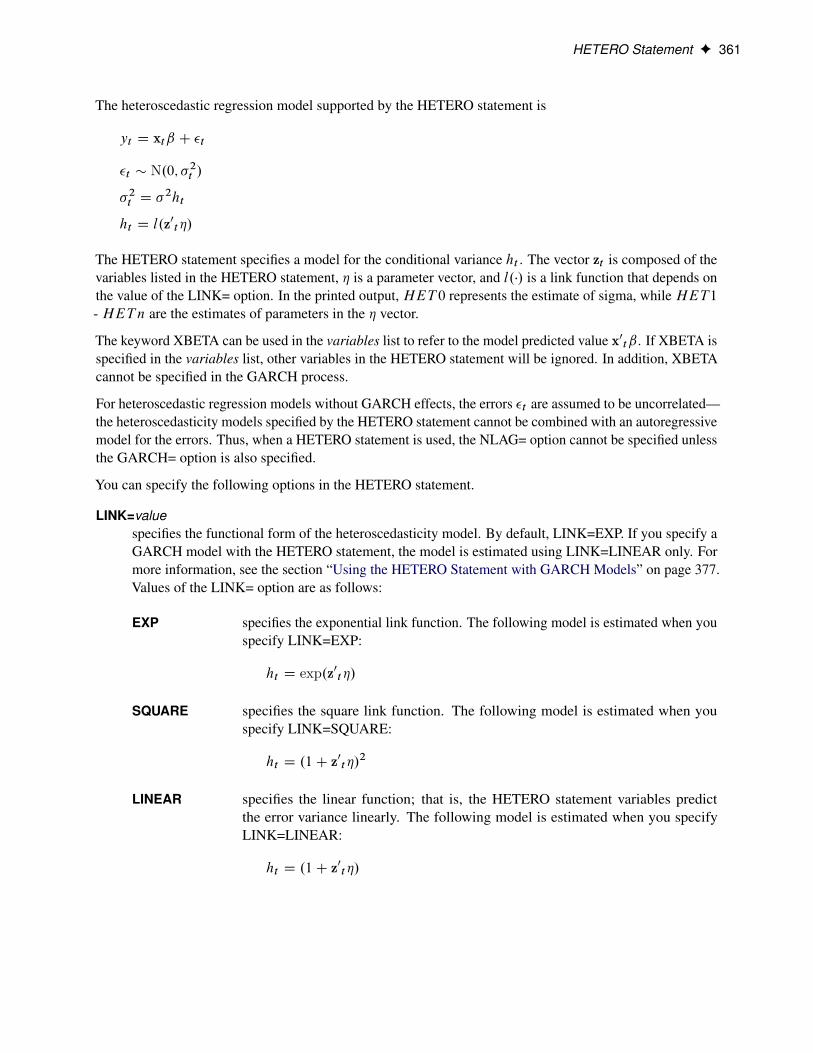
HETERO Statement F 361
The heteroscedastic regression model supported by the HETERO statement is
yt D xtˇ C �t
�t � N.0; �2t /
�2t D �2ht
ht D l.z0t�/
The HETERO statement specifies a model for the conditional variance ht . The vector zt is composed of thevariables listed in the HETERO statement, � is a parameter vector, and l.�/ is a link function that depends onthe value of the LINK= option. In the printed output, HET 0 represents the estimate of sigma, while HET1- HETn are the estimates of parameters in the � vector.
The keyword XBETA can be used in the variables list to refer to the model predicted value x0tˇ. If XBETA isspecified in the variables list, other variables in the HETERO statement will be ignored. In addition, XBETAcannot be specified in the GARCH process.
For heteroscedastic regression models without GARCH effects, the errors �t are assumed to be uncorrelated—the heteroscedasticity models specified by the HETERO statement cannot be combined with an autoregressivemodel for the errors. Thus, when a HETERO statement is used, the NLAG= option cannot be specified unlessthe GARCH= option is also specified.
You can specify the following options in the HETERO statement.
LINK=valuespecifies the functional form of the heteroscedasticity model. By default, LINK=EXP. If you specify aGARCH model with the HETERO statement, the model is estimated using LINK=LINEAR only. Formore information, see the section “Using the HETERO Statement with GARCH Models” on page 377.Values of the LINK= option are as follows:
EXP specifies the exponential link function. The following model is estimated when youspecify LINK=EXP:
ht D exp.z0t�/
SQUARE specifies the square link function. The following model is estimated when youspecify LINK=SQUARE:
ht D .1C z0t�/2
LINEAR specifies the linear function; that is, the HETERO statement variables predictthe error variance linearly. The following model is estimated when you specifyLINK=LINEAR:
ht D .1C z0t�/

362 F Chapter 8: The AUTOREG Procedure
COEF=valueimposes constraints on the estimated parameters � of the heteroscedasticity model. You can specifythe following values:
NONNEG specifies that the estimated heteroscedasticity parameters � must be nonnegative.
UNIT constrains all heteroscedasticity parameters � to equal 1.
ZERO constrains all heteroscedasticity parameters � to equal 0.
UNREST specifies unrestricted estimation of �.
If you specify the GARCH= option in the MODEL statement, the default is COEF=NONNEG. If youdo not specify the GARCH= option in the MODEL statement, the default is COEF=UNREST.
STD=valueimposes constraints on the estimated standard deviation � of the heteroscedasticity model. You canspecify the following values:
NONNEG specifies that the estimated standard deviation parameter � must be nonnegative.
UNIT constrains the standard deviation parameter � to equal 1.
UNREST specifies unrestricted estimation of � .
The default is STD=UNREST.
TEST=LMproduces a Lagrange multiplier test for heteroscedasticity. The null hypothesis is homoscedasticity;the alternative hypothesis is heteroscedasticity of the form specified by the HETERO statement. Thepower of the test depends on the variables specified in the HETERO statement.
The test may give different results depending on the functional form specified by the LINK= option.However, in many cases the test does not depend on the LINK= option. The test is invariant to theform of ht when ht .0/ D 1 and h0t .0/ ¤ 0. (The condition ht .0/ D 1 is satisfied except when theNOCONST option is specified with LINK=SQUARE or LINK=LINEAR.)
NOCONSTspecifies that the heteroscedasticity model does not include the unit term for the LINK=SQUARE andLINK=LINEAR options. For example, the following model is estimated when you specify the optionsLINK=SQUARE NOCONST:
ht D .z0t�/2
NLOPTIONS StatementNLOPTIONS < options > ;
PROC AUTOREG uses the nonlinear optimization (NLO) subsystem to perform nonlinear optimization taskswhen the GARCH= option is specified. If the GARCH= option is not specified, the NLOPTIONS statementis ignored. For a list of all the options of the NLOPTIONS statement, see Chapter 6, “Nonlinear OptimizationMethods.”

OUTPUT Statement F 363
For the TECHNIQUE= option in the NLOPTIONS statement, only the QUANEW and TRUREG methodsare supported, corresponding to the OPTMETHOD=QN and TR in the MODEL statement, respectively.
OUTPUT StatementOUTPUT < OUT=SAS-data-set > < options > < keyword=name > ;
The OUTPUT statement creates an output SAS data set as specified by the following options.
OUT=SAS-data-setnames the output SAS data set to contain the predicted and transformed values. If the OUT= option isnot specified, the new data set is named according to the DATAn convention.
You can specify any of the following options:
ALPHACLI=numbersets the confidence limit size for the estimates of future values of the response time series. TheALPHACLI= value must be between 0 and 1. The resulting confidence interval has 1–numberconfidence. The default is ALPHACLI=0.05, which corresponds to a 95% confidence interval.
ALPHACLM=numbersets the confidence limit size for the estimates of the structural or regression part of the model. TheALPHACLM= value must be between 0 and 1. The resulting confidence interval has 1–numberconfidence. The default is ALPHACLM=0.05, which corresponds to a 95% confidence interval.
ALPHACSM=0.01 | 0.05 | 0.10specifies the significance level for the upper and lower bounds of the CUSUM and CUSUMSQstatistics output by the CUSUMLB=, CUSUMUB=, CUSUMSQLB=, and CUSUMSQUB= options.The significance level specified by the ALPHACSM= option can be 0.01, 0.05, or 0.10. Other valuesare not supported.
You can specify the following values for keyword=name, where keyword specifies the statistic to include inthe output data set and name gives the name of the variable in the OUT= data set to contain the statistic.
BLUS=variablespecifies the name of a variable to contain the values of the Theil’s BLUS residuals. For moreinformation about BLUS residuals, see Theil (1971).
CEV=variable
HT=variablewrites to the output data set the value of the error variance �2t from the heteroscedasticity modelspecified by the HETERO statement or the value of the conditional error variance ht by the GARCH=option in the MODEL statement.
CPEV=variablewrites the conditional prediction error variance to the output data set. The value of conditional predic-tion error variance is equal to that of the conditional error variance when there are no autoregressiveparameters. For more information, see the section “Predicted Values” on page 409.

364 F Chapter 8: The AUTOREG Procedure
CONSTANT=variablewrites the transformed intercept to the output data set. For information about the transformation, seethe section “Computational Methods” on page 370.
CUSUM=variablespecifies the name of a variable to contain the CUSUM statistics.
CUSUMSQ=variablespecifies the name of a variable to contain the CUSUMSQ statistics.
CUSUMUB=variablespecifies the name of a variable to contain the upper confidence bound for the CUSUM statistic.
CUSUMLB=variablespecifies the name of a variable to contain the lower confidence bound for the CUSUM statistic.
CUSUMSQUB=variablespecifies the name of a variable to contain the upper confidence bound for the CUSUMSQ statistic.
CUSUMSQLB=variablespecifies the name of a variable to contain the lower confidence bound for the CUSUMSQ statistic.
LCL=namewrites the lower confidence limit for the predicted value (specified in the PREDICTED= option) tothe output data set. The size of the confidence interval is set by the ALPHACLI= option. For moreinformation, see the section “Predicted Values” on page 409.
LCLM=namewrites the lower confidence limit for the structural predicted value (specified in the PREDICTEDM=option) to the output data set under the name given. The size of the confidence interval is set by theALPHACLM= option.
PREDICTED=name
P=namewrites the predicted values to the output data set. These values are formed from both the structuraland autoregressive parts of the model. For more information, see the section “Predicted Values” onpage 409.
PREDICTEDM=name
PM=namewrites the structural predicted values to the output data set. These values are formed from only thestructural part of the model. For more information, see the section “Predicted Values” on page 409.
RECPEV=variablespecifies the name of a variable to contain the part of the predictive error variance (vt ) that is used tocompute the recursive residuals.
RECRES=variablespecifies the name of a variable to contain recursive residuals. The recursive residuals are used tocompute the CUSUM and CUSUMSQ statistics.

RESTRICT Statement F 365
RESIDUAL=name
R=namewrites the residuals from the predicted values based on both the structural and time series parts of themodel to the output data set.
RESIDUALM=name
RM=namewrites the residuals from the structural prediction to the output data set.
STDERR=name
SE=namewrites the standard errors of the predicted values to the data set that is specified in the OUT= option.
STDERRM=name
SEM=namewrites the standard errors of the structural predicted values to the data set that is specified in the OUT=option.
TRANSFORM=variablestransforms the specified variables from the input data set by the autoregressive model and writes thetransformed variables to the output data set. For information about the transformation, see the section“Computational Methods” on page 370. If you need to reproduce the data suitable for re-estimation,you must also transform an intercept variable. To do this, transform a variable that is all 1s or use theCONSTANT= option.
UCL=namewrites the upper confidence limit for the predicted value (specified in the PREDICTED= option) tothe output data set. The size of the confidence interval is set by the ALPHACLI= option. For moreinformation, see the section “Predicted Values” on page 409.
UCLM=namewrites the upper confidence limit for the structural predicted value (specified in the PREDICTEDM=option) to the output data set. The size of the confidence interval is set by the ALPHACLM= option.
RESTRICT StatementRESTRICT equation , . . . , equation ;
The RESTRICT statement provides constrained estimation and places restrictions on the parameter estimatesfor covariates in the preceding MODEL statement. The AR, GARCH, and HETERO parameters are alsosupported in the RESTRICT statement when you specify the GARCH= option. Any number of RESTRICTstatements can follow a MODEL statement. To specify more than one restriction in a single RESTRICTstatement, separate them with commas.
Each restriction is written as a linear equation composed of constants and parameter names. Refer to modelparameters by the name of the corresponding regressor variable. Each name that is used in the equationmust be a regressor in the preceding MODEL statement. Use the keyword INTERCEPT to refer to theintercept parameter in the model. For the names of these parameters, see the section “OUTEST= Data Set” on

366 F Chapter 8: The AUTOREG Procedure
page 413. Inequality constraints are supported only when you specify the GARCH= option. For non-GARCHmodels, if inequality signs are specified, they are treated as equality signs.
Lagrange multipliers are reported in the “Parameter Estimates” table for all the active linear constraints. Theyare identified by the names Restrict1, Restrict2, and so on. The probabilities of these Lagrange multipliersare computed using a beta distribution (LaMotte 1994). Nonactive (nonbinding) restrictions have no effecton the estimation results and are not noted in the output.
The following is an example of a RESTRICT statement:
model y = a b c d;restrict a+b=0, 2*d-c=0;
When restricting a linear combination of parameters to be 0, you can omit the equal sign. For example, thefollowing RESTRICT statement is equivalent to the preceding example:
restrict a+b, 2*d-c;
The following RESTRICT statement constrains the parameters estimates for three regressors (X1, X2, andX3) to be equal:
restrict x1 = x2, x2 = x3;
The preceding restriction can be abbreviated as follows:
restrict x1 = x2 = x3;
The following example shows how to specify AR, GARCH, and HETERO parameters in the RESTRICTstatement:
model y = a b / nlag=2 garch=(p=2,q=3,mean=sqrt);hetero c d;restrict _A_1=0,_AH_2=0.2,_HET_2=1,_DELTA_=0.1;
You can specify only simple linear combinations of parameters in RESTRICT statement expressions. Youcannot specify complex expressions that involve parentheses, division, functions, or complex products.
TEST StatementThe AUTOREG procedure supports a TEST statement for linear hypothesis tests. The syntax of the TESTstatement is
TEST equation , . . . , equation / option ;
The TEST statement tests hypotheses about the covariates in the model that are estimated by the precedingMODEL statement. The AR, GARCH, and HETERO parameters are also supported in the TEST statementwhen you specify the GARCH= option. Each equation specifies a linear hypothesis to be tested. If youspecify more than one equation, separate them with commas.
Each test is written as a linear equation composed of constants and parameter names. Refer to parameters bythe name of the corresponding regressor variable. Each name that is used in the equation must be a regressorin the preceding MODEL statement. Use the keyword INTERCEPT to refer to the intercept parameter in themodel. For the names of these parameters, see the section “OUTEST= Data Set” on page 413.
You can specify the following options in the TEST statement:

TEST Statement F 367
TYPE=valuespecifies the test statistics to use. The default is TYPE=F. The following values for the TYPE= optionare available:
F produces an F test. This option is supported for all models specified in the MODELstatement.
WALD produces a Wald test. This option is supported for all models specified in theMODEL statement.
LM produces a Lagrange multiplier test. This option is supported only when theGARCH= option is specified (for example, when there is a statement like MODELY = C D I / GARCH=(Q=2)).
LR produces a likelihood ratio test. This option is supported only when the GARCH=option is specified (for example, when there is a statement like MODEL Y = C D I/ GARCH=(Q=2)).
ALL produces all tests applicable for a particular model. For non-GARCH-type models,only F and Wald tests are output. For all other models, all four tests (LR, LM, F,and Wald) are computed.
The following example of a TEST statement tests the hypothesis that the coefficients of two regressors A andB are equal:
model y = a b c d;test a = b;
To test separate null hypotheses, use separate TEST statements. To test a joint hypothesis, specify thecomponent hypotheses on the same TEST statement, separated by commas.
For example, consider the following linear model:
yt D ˇ0 C ˇ1x1t C ˇ2x2t C �t
The following statements test the two hypotheses H0 W ˇ0 D 1 and H0 W ˇ1 C ˇ2 D 0:
model y = x1 x2;test intercept = 1;test x1 + x2 = 0;
The following statements test the joint hypothesis H0 W ˇ0 D 1 and ˇ1 C ˇ2 D 0:
model y = x1 x2;test intercept = 1, x1 + x2 = 0;
To illustrate the TYPE= option, consider the following examples:
model Y = C D I / garch=(q=2);test C + D = 1;
The preceding statements produce only one default test, the F test.

368 F Chapter 8: The AUTOREG Procedure
model Y = C D I / garch=(q=2);test C + D = 1 / type = LR;
The preceding statements produce one of four tests applicable for GARCH-type models, the likelihood ratiotest.
model Y = C D I / nlag = 2;test C + D = 1 / type = LM;
The preceding statements produce the warning and do not output any test because the Lagrange multipliertest is not applicable for non-GARCH models.
model Y = C D I / nlag=2;test C + D = 1 / type = ALL;
The preceding statements produce all tests that are applicable for non-GARCH models (namely, the F andWald tests). The TYPE= prefix is optional. Thus the test statement in the previous example could also havebeen written as
test C + D = 1 / ALL;
The following example shows how to test AR, GARCH, and HETERO parameters:
model y = a b / nlag=2 garch=(p=2,q=3,mean=sqrt);hetero c d;test _A_1=0,_AH_2=0.2,_HET_2=1,_DELTA_=0.1;
Details: AUTOREG Procedure
Missing ValuesPROC AUTOREG skips any missing values at the beginning of the data set. If the NOMISS option isspecified, the first contiguous set of data with no missing values is used; otherwise, all data with nonmissingvalues for the independent and dependent variables are used. Note, however, that the observations containingmissing values are still needed to maintain the correct spacing in the time series. PROC AUTOREG cangenerate predicted values when the dependent variable is missing.
Autoregressive Error ModelThe regression model with autocorrelated disturbances is as follows:
yt D x0tˇ C �t
�t D �t � '1�t�1 � � � � � 'm�t�m
�t N.0; �2/

Autoregressive Error Model F 369
In these equations, yt are the dependent values, xt is a column vector of regressor variables, ˇ is a columnvector of structural parameters, and �t is normally and independently distributed with a mean of 0 and avariance of �2. Note that in this parameterization, the signs of the autoregressive parameters are reversedfrom the parameterization documented in most of the literature.
PROC AUTOREG offers four estimation methods for the autoregressive error model. The default method,Yule-Walker (YW) estimation, is the fastest computationally. The Yule-Walker method used by PROCAUTOREG is described in Gallant and Goebel (1976). Harvey (1981) calls this method the two-step fulltransform method. The other methods are iterated YW, unconditional least squares (ULS), and maximumlikelihood (ML). The ULS method is also referred to as nonlinear least squares (NLS) or exact least squares(ELS).
You can use all of the methods with data containing missing values, but you should use ML estimation if themissing values are plentiful. For further discussion of the advantages of different methods, see the section“Alternative Autocorrelation Correction Methods” on page 372, later in this chapter.
The Yule-Walker Method
Let ' represent the vector of autoregressive parameters,
' D .'1; '2; : : : ; 'm/0
and let the variance matrix of the error vector � D .�1; : : : ; �N /0 be †,
E.��0/ D † D �2V
If the vector of autoregressive parameters ' is known, the matrix V can be computed from the autoregressiveparameters. † is then �2V. Given †, the efficient estimates of regression parameters ˇ can be computedusing generalized least squares (GLS). The GLS estimates then yield the unbiased estimate of the variance�2,
The Yule-Walker method alternates estimation of ˇ using generalized least squares with estimation of ' usingthe Yule-Walker equations applied to the sample autocorrelation function. The YW method starts by formingthe OLS estimate of ˇ. Next, ' is estimated from the sample autocorrelation function of the OLS residualsby using the Yule-Walker equations. Then V is estimated from the estimate of ', and † is estimated from Vand the OLS estimate of �2. The autocorrelation corrected estimates of the regression parameters ˇ are thencomputed by GLS, using the estimated † matrix. These are the Yule-Walker estimates.
If the ITER option is specified, the Yule-Walker residuals are used to form a new sample autocorrelationfunction, the new autocorrelation function is used to form a new estimate of ' and V, and the GLS estimatesare recomputed using the new variance matrix. This alternation of estimates continues until either themaximum change in theb' estimate between iterations is less than the value specified by the CONVERGE=option or the maximum number of allowed iterations is reached. This produces the iterated Yule-Walkerestimates. Iteration of the estimates may not yield much improvement.
The Yule-Walker equations, solved to obtainb' and a preliminary estimate of �2, are
R O' D �r
Here r D .r1; : : : ; rm/0, where ri is the lag i sample autocorrelation. The matrix R is the Toeplitz matrixwhose i,jth element is rji�j j. If you specify a subset model, then only the rows and columns of R and rcorresponding to the subset of lags specified are used.
370 F Chapter 8: The AUTOREG Procedure
If the BACKSTEP option is specified, for purposes of significance testing, the matrix ŒR r� is treated as asum-of-squares-and-crossproducts matrix arising from a simple regression with N � k observations, where kis the number of estimated parameters.
The Unconditional Least Squares and Maximum Likelihood Methods
Define the transformed error, e D .�1; : : : ; �T /, as
e D L�1n
where n D y �Xˇ and L is the Cholesky root of V—that is, V D LL0 with L lower triangular..
The unconditional sum of squares for the model, S, is
S D n0V�1n D e0e
The ULS estimates are computed by minimizing S with respect to the parameters ˇ and 'i .
The full log-likelihood function for the autoregressive error model is
l D �N
2ln.2�/ �
N
2ln.�2/ �
1
2ln.jVj/ �
S
2�2
where jVj denotes determinant of V. For the ML method, the likelihood function is maximized by minimizingan equivalent sum-of-squares function.
Maximizing l with respect to �2 (and concentrating �2 out of the likelihood) and dropping the constant term�N2
ln.2�/C 1 � ln.N / produces the concentrated log-likelihood function
lc D �N
2ln.S jVj1=N /
Rewriting the variable term within the logarithm gives
Sml D jLj1=N e0ejLj1=N
PROC AUTOREG computes the ML estimates by minimizing the objective function Sml D jLj1=N e0ejLj1=N .
The maximum likelihood estimates may not exist for some data sets (Anderson and Mentz 1980). This is thecase for very regular data sets, such as an exact linear trend.
Computational Methods
Sample Autocorrelation FunctionThe sample autocorrelation function is computed from the structural residuals or noise nt D yt � x0tb, whereb is the current estimate of ˇ. The sample autocorrelation function is the sum of all available lagged productsof nt of order j divided by `C j , where ` is the number of such products.
If there are no missing values, then `C j D N , the number of observations. In this case, the Toeplitz matrixof autocorrelations, R, is at least positive semidefinite. If there are missing values, these autocorrelationestimates of r can yield an R matrix that is not positive semidefinite. If such estimates occur, a warningmessage is printed, and the estimates are tapered by exponentially declining weights until R is positivedefinite.
Autoregressive Error Model F 371
Data Transformation and the Kalman FilterThe calculation of V from ' for the general AR.m/ model is complicated, and the size of V depends on thenumber of observations. Instead of actually calculating V and performing GLS in the usual way, in practicea Kalman filter algorithm is used to transform the data and compute the GLS results through a recursiveprocess.
In all of the estimation methods, the original data are transformed by the inverse of the Cholesky root ofV. Let L denote the Cholesky root of V—that is, V D LL0 with L lower triangular. For an AR.m/ model,L�1 is a band diagonal matrix with m anomalous rows at the beginning and the autoregressive parametersalong the remaining rows. Thus, if there are no missing values, after the first m � 1 observations the data aretransformed as
zt D xt C O'1xt�1 C � � � C O'mxt�m
The transformation is carried out using a Kalman filter, and the lower triangular matrix L is never directlycomputed. The Kalman filter algorithm, as it applies here, is described in Harvey and Phillips (1979) andJones (1980). Although L is not computed explicitly, for ease of presentation the remaining discussion isin terms of L. If there are missing values, then the submatrix of L consisting of the rows and columns withnonmissing values is used to generate the transformations.
Gauss-Newton AlgorithmsThe ULS and ML estimates employ a Gauss-Newton algorithm to minimize the sum of squares and maximizethe log likelihood, respectively. The relevant optimization is performed simultaneously for both the regressionand AR parameters. The OLS estimates of ˇ and the Yule-Walker estimates of ' are used as starting valuesfor these methods.
The Gauss-Newton algorithm requires the derivatives of e or jLj1=N e with respect to the parameters. Thederivatives with respect to the parameter vector ˇ are
@e@ˇ0D �L�1X
@jLj1=N e@ˇ0
D �jLj1=NL�1X
These derivatives are computed by the transformation described previously. The derivatives with respect to 'are computed by differentiating the Kalman filter recurrences and the equations for the initial conditions.
Variance Estimates and Standard Errors
For the Yule-Walker method, the estimate of the error variance, s2, is the error sum of squares from the lastapplication of GLS, divided by the error degrees of freedom (number of observations N minus the number offree parameters).
The variance-covariance matrix for the components of b is taken as s2.X0V�1X/�1 for the Yule-Walkermethod. For the ULS and ML methods, the variance-covariance matrix of the parameter estimates is computedas s2.J0J/�1. For the ULS method, J is the matrix of derivatives of e with respect to the parameters. Forthe ML method, J is the matrix of derivatives of jLj1=N e divided by jLj1=N . The estimate of the variance-covariance matrix of b assuming that ' is known is s2.X0V�1X/�1. For OLS model, the estimate of thevariance-covariance matrix is s2.X0X/�1.

372 F Chapter 8: The AUTOREG Procedure
Park and Mitchell (1980) investigated the small sample performance of the standard error estimates obtainedfrom some of these methods. In particular, simulating an AR(1) model for the noise term, they found that thestandard errors calculated using GLS with an estimated autoregressive parameter underestimated the truestandard errors. These estimates of standard errors are the ones calculated by PROC AUTOREG with theYule-Walker method.
The estimates of the standard errors calculated with the ULS or ML method take into account the jointestimation of the AR and the regression parameters and may give more accurate standard-error values thanthe YW method. At the same values of the autoregressive parameters, the ULS and ML standard errorswill always be larger than those computed from Yule-Walker. However, simulations of the models used byPark and Mitchell (1980) suggest that the ULS and ML standard error estimates can also be underestimates.Caution is advised, especially when the estimated autocorrelation is high and the sample size is small.
High autocorrelation in the residuals is a symptom of lack of fit. An autoregressive error model should not beused as a nostrum for models that simply do not fit. It is often the case that time series variables tend to moveas a random walk. This means that an AR(1) process with a parameter near one absorbs a great deal of thevariation. See Example 8.3, which fits a linear trend to a sine wave.
For ULS or ML estimation, the joint variance-covariance matrix of all the regression and autoregressionparameters is computed. For the Yule-Walker method, the variance-covariance matrix is computed only forthe regression parameters.
Lagged Dependent Variables
The Yule-Walker estimation method is not directly appropriate for estimating models that include laggeddependent variables among the regressors. Therefore, the maximum likelihood method is the default whenthe LAGDEP or LAGDEP= option is specified in the MODEL statement. However, when lagged dependentvariables are used, the maximum likelihood estimator is not exact maximum likelihood but is conditional onthe first few values of the dependent variable.
Alternative Autocorrelation Correction MethodsAutocorrelation correction in regression analysis has a long history, and various approaches have beensuggested. Moreover, the same method may be referred to by different names.
Pioneering work in the field was done by Cochrane and Orcutt (1949). The Cochrane-Orcutt method refersto a more primitive version of the Yule-Walker method that drops the first observation. The Cochrane-Orcuttmethod is like the Yule-Walker method for first-order autoregression, except that the Yule-Walker methodretains information from the first observation. The iterative Cochrane-Orcutt method is also in use.
The Yule-Walker method used by PROC AUTOREG is also known by other names. Harvey (1981) refers tothe Yule-Walker method as the two-step full transform method. The Yule-Walker method can be consideredas generalized least squares using the OLS residuals to estimate the covariances across observations, andJudge et al. (1985) use the term estimated generalized least squares (EGLS) for this method. For a first-orderAR process, the Yule-Walker estimates are often termed Prais-Winsten estimates (Prais and Winsten 1954).There are variations to these methods that use different estimators of the autocorrelations or the autoregressiveparameters.
The unconditional least squares (ULS) method, which minimizes the error sum of squares for all observations,is referred to as the nonlinear least squares (NLS) method by Spitzer (1979).

GARCH Models F 373
The Hildreth-Lu method (Hildreth and Lu 1960) uses nonlinear least squares to jointly estimate the parameterswith an AR(1) model, but it omits the first transformed residual from the sum of squares. Thus, the Hildreth-Lu method is a more primitive version of the ULS method supported by PROC AUTOREG in the same wayCochrane-Orcutt is a more primitive version of Yule-Walker.
The maximum likelihood method is also widely cited in the literature. Although the maximum likelihoodmethod is well defined, some early literature refers to estimators that are called maximum likelihood but arenot full unconditional maximum likelihood estimates. The AUTOREG procedure produces full unconditionalmaximum likelihood estimates.
Harvey (1981) and Judge et al. (1985) summarize the literature on various estimators for the autoregressiveerror model. Although asymptotically efficient, the various methods have different small sample properties.Several Monte Carlo experiments have been conducted, although usually for the AR(1) model.
Harvey and McAvinchey (1978) found that for a one-variable model, when the independent variable istrending, methods similar to Cochrane-Orcutt are inefficient in estimating the structural parameter. This is notsurprising since a pure trend model is well modeled by an autoregressive process with a parameter close to 1.
Harvey and McAvinchey (1978) also made the following conclusions:
� The Yule-Walker method appears to be about as efficient as the maximum likelihood method. AlthoughSpitzer (1979) recommended ML and NLS, the Yule-Walker method (labeled Prais-Winsten) did aswell or better in estimating the structural parameter in Spitzer’s Monte Carlo study (table A2 in theirarticle) when the autoregressive parameter was not too large. Maximum likelihood tends to do betterwhen the autoregressive parameter is large.
� For small samples, it is important to use a full transformation (Yule-Walker) rather than the Cochrane-Orcutt method, which loses the first observation. This was also demonstrated by Maeshiro (1976),Chipman (1979), and Park and Mitchell (1980).
� For large samples (Harvey and McAvinchey used 100), losing the first few observations does not makemuch difference.
GARCH ModelsConsider the series yt , which follows the GARCH process. The conditional distribution of the series Y fortime t is written
yt j‰t�1�N.0; ht /
where ‰t�1 denotes all available information at time t � 1. The conditional variance ht is
ht D ! C
qXiD1
˛iy2t�i C
pXjD1
jht�j
where
p � 0; q > 0
374 F Chapter 8: The AUTOREG Procedure
! > 0; ˛i � 0; j � 0
The GARCH.p; q/ model reduces to the ARCH.q/ process when p D 0. At least one of the ARCHparameters must be nonzero (q > 0). The GARCH regression model can be written
yt D x0tˇ C �t
�t Dphtet
ht D ! C
qXiD1
˛i�2t�i C
pXjD1
jht�j
where �t�IN.0; 1/.
In addition, you can consider the model with disturbances following an autoregressive process and with theGARCH errors. The AR.m/-GARCH.p; q/ regression model is denoted
yt D x0tˇ C �t
�t D �t � '1�t�1 � � � � � 'm�t�m
�t Dphtet
ht D ! C
qXiD1
˛i�2t�i C
pXjD1
jht�j
GARCH Estimation with Nelson-Cao Inequality Constraints
The GARCH.p; q/ model is written in ARCH(1) form as
ht D
0@1 � pXjD1
jBj
1A�1 "! C qXiD1
˛i�2t�i
#
D !� C
1XiD1
�i�2t�i
where B is a backshift operator. Therefore, ht � 0 if !� � 0 and �i � 0; 8i . Assume that the roots of thefollowing polynomial equation are inside the unit circle,
pXjD0
� jZp�j
where 0 D �1 and Z is a complex scalar. �PpjD0 jZ
p�j andPqiD1 ˛iZ
q�i do not share commonfactors. Under these conditions, j!�j <1, j�i j <1, and these coefficients of the ARCH(1) process arewell defined.
GARCH Models F 375
Define n D max.p; q/. The coefficient �i is written
�0 D ˛1
�1 D 1�0 C ˛2
� � �
�n�1 D 1�n�2 C 2�n�3 C � � � C n�1�0 C ˛n
�k D 1�k�1 C 2�k�2 C � � � C n�k�n for k � n
where ˛i D 0 for i > q and j D 0 for j > p.
Nelson and Cao (1992) proposed the finite inequality constraints for GARCH.1; q/ and GARCH.2; q/ cases.However, it is not straightforward to derive the finite inequality constraints for the general GARCH.p; q/model.
For the GARCH.1; q/ model, the nonlinear inequality constraints are
! � 0
1 � 0
�k � 0 for k D 0; 1; : : : ; q � 1
For the GARCH.2; q/ model, the nonlinear inequality constraints are
�i 2 R for i D 1; 2
!� � 0
�1 > 0q�1XjD0
��j1 ˛jC1 > 0
�k � 0 for k D 0; 1; : : : ; q
where �1 and �2 are the roots of .Z 2 � 1Z � 2/.
For the GARCH.p; q/ model with p > 2, only max.q � 1; p/C 1 nonlinear inequality constraints (�k � 0for k D 0 to max(q � 1; p)) are imposed, together with the in-sample positivity constraints of the conditionalvariance ht .
IGARCH and Stationary GARCH Model
The conditionPqiD1 ˛i C
PpjD1 j < 1 implies that the GARCH process is weakly stationary since the
mean, variance, and autocovariance are finite and constant over time. When the GARCH process is stationary,the unconditional variance of �t is computed as
V.�t / D!
.1 �PqiD1 ˛i �
PpjD1 j /
where �t Dphtet and ht is the GARCH.p; q/ conditional variance.
Sometimes the multistep forecasts of the variance do not approach the unconditional variance when themodel is integrated in variance; that is,
PqiD1 ˛i C
PpjD1 j D 1.
376 F Chapter 8: The AUTOREG Procedure
The unconditional variance for the IGARCH model does not exist. However, it is interesting that the IGARCHmodel can be strongly stationary even though it is not weakly stationary. For more information, see Nelson(1990).
EGARCH Model
The EGARCH model was proposed by Nelson (1991). Nelson and Cao (1992) argue that the nonnegativityconstraints in the linear GARCH model are too restrictive. The GARCH model imposes the nonnegativeconstraints on the parameters, ˛i and j , while there are no restrictions on these parameters in the EGARCHmodel. In the EGARCH model, the conditional variance, ht , is an asymmetric function of lagged disturbances�t�i ,
ln.ht / D ! CqXiD1
˛ig.zt�i /C
pXjD1
j ln.ht�j /
where
g.zt / D �zt C Œjzt j �Ejzt j�
zt D �t=pht
The coefficient of the second term in g.zt / is set to be 1 ( =1) in our formulation. Note thatEjzt j D .2=�/1=2
if zt�N.0; 1/. The properties of the EGARCH model are summarized as follows:
� The function g.zt / is linear in zt with slope coefficient � C 1 if zt is positive while g.zt / is linear inzt with slope coefficient � � 1 if zt is negative.
� Suppose that � D 0. Large innovations increase the conditional variance if jzt j �Ejzt j > 0 anddecrease the conditional variance if jzt j �Ejzt j < 0.
� Suppose that � < 1. The innovation in variance, g.zt /, is positive if the innovations zt are less than.2=�/1=2=.� � 1/. Therefore, the negative innovations in returns, �t , cause the innovation to theconditional variance to be positive if � is much less than 1.
QGARCH, TGARCH, and PGARCH Models
As shown in many empirical studies, positive and negative innovations have different impacts on future volatil-ity. There is a long list of variations of GARCH models that consider the asymmetricity. Three typical varia-tions are the quadratic GARCH (QGARCH) model (Engle and Ng 1993), the threshold GARCH (TGARCH)model (Glosten, Jaganathan, and Runkle 1993; Zakoian 1994), and the power GARCH (PGARCH) model(Ding, Granger, and Engle 1993). For more information about the asymmetric GARCH models, see Engleand Ng (1993).
In the QGARCH model, the lagged errors’ centers are shifted from zero to some constant values:
ht D ! C
qXiD1
˛i .�t�i � i /2C
pXjD1
jht�j

GARCH Models F 377
In the TGARCH model, there is an extra slope coefficient for each lagged squared error,
ht D ! C
qXiD1
.˛i C 1�t�i<0 i /�2t�i C
pXjD1
jht�j
where the indicator function 1�t<0 is one if �t < 0; otherwise, zero.
The PGARCH model not only considers the asymmetric effect, but also provides another way to model thelong memory property in the volatility,
h�t D ! C
qXiD1
˛i .j�t�i j � i�t�i /2�C
pXjD1
jh�t�j
where � > 0 and j i j � 1; i D 1; : : : ; q.
Note that the implemented TGARCH model is also well known as GJR-GARCH (Glosten, Jaganathan, andRunkle 1993), which is similar to the threshold GARCH model proposed by Zakoian (1994) but not exactlythe same. In Zakoian’s model, the conditional standard deviation is a linear function of the past values of thewhite noise. Zakoian’s version can be regarded as a special case of the PGARCH model when � D 1=2.
Using the HETERO Statement with GARCH Models
The HETERO statement can be combined with the GARCH= option in the MODEL statement to includeinput variables in the GARCH conditional variance model. For example, the GARCH.1; 1/ variance modelwith two dummy input variables, D1 and D2, is
�t Dphtet
ht D ! C ˛1�2t�1 C 1ht�1 C �1D1t C �2D2t
The following statements estimate this GARCH model:
proc autoreg data=one;model y = x z / garch=(p=1,q=1);hetero d1 d2;
run;
The parameters for the variables D1 and D2 can be constrained using the COEF= option. For example, theconstraints �1 D �2 D 1 are imposed by the following statements:
proc autoreg data=one;model y = x z / garch=(p=1,q=1);hetero d1 d2 / coef=unit;
run;
For the EGARCH model, the input variables enter ln.ht /. For example, the EGARCH.1; 1/ model with twodummy input variables, D1 and D2, is
ln.ht / D ! C ˛1g.zt�1/C 1ln.ht�1/C �1D1t C �2D2t

378 F Chapter 8: The AUTOREG Procedure
where
g.zt / D �zt C Œjzt j �Ejzt j�
zt D �t=pht
The following statements estimate the EGARCH model:
proc autoreg data=one;model y = x z / garch=(p=1,q=1,type=egarch);hetero d1 d2;
run;
For the PGARCH model, the input variables enter h�t . For example, the PGARCH.1; 1/ model with twodummy input variables, D1 and D2, is
h�t D ! C ˛1.j�t�1j � 1�t�1/2�C jh
�t�j C �1D1t C �2D2t
The following statements estimate the PGARCH model:
proc autoreg data=one;model y = x z / garch=(p=1,q=1,type=pgarch);hetero d1 d2;
run;
GARCH-in-Mean
The GARCH-M model has the added regressor that is the conditional standard deviation,
yt D x0tˇ C ıpht C �t
�t Dphtet
where ht follows the ARCH or GARCH process.
Maximum Likelihood Estimation
The family of GARCH models are estimated using the maximum likelihood method. The log-likelihoodfunction is computed from the product of all conditional densities of the prediction errors.
When et is assumed to have a standard normal distribution (et�N.0; 1/), the log-likelihood function is givenby
l D
NXtD1
1
2
��ln.2�/ � ln.ht / �
�2tht
�where �t D yt � x0tˇ and ht is the conditional variance. When the GARCH.p; q/-M model is estimated,�t D yt � x0tˇ � ı
pht . When there are no regressors, the residuals �t are denoted as yt or yt � ı
pht .
If et has the standardized Student’s t distribution, the log-likelihood function for the conditional t distributionis
` D
NXtD1
"ln��
�� C 1
2
��� ln
����2
���1
2ln..� � 2/�ht /

Heteroscedasticity- and Autocorrelation-Consistent Covariance Matrix Estimator F 379
�1
2.� C 1/ln
�1C
�2tht .� � 2/
�#where �.�/ is the gamma function and � is the degree of freedom (� > 2). Under the conditional t distribution,the additional parameter 1=� is estimated. The log-likelihood function for the conditional t distributionconverges to the log-likelihood function of the conditional normal GARCH model as 1=�! 0.
The likelihood function is maximized via either the dual quasi-Newton or the trust region algorithm. Thedefault is the dual quasi-Newton algorithm. The starting values for the regression parameters ˇ are obtainedfrom the OLS estimates. When there are autoregressive parameters in the model, the initial values are obtainedfrom the Yule-Walker estimates. The starting value 1:0�6 is used for the GARCH process parameters.
The variance-covariance matrix is computed using the Hessian matrix. The dual quasi-Newton methodapproximates the Hessian matrix while the quasi-Newton method gets an approximation of the inverse ofHessian. The trust region method uses the Hessian matrix obtained using numerical differentiation. Whenthere are active constraints, that is, q.�/ D 0, the variance-covariance matrix is given by
V. O�/ D H�1ŒI �Q0.QH�1Q0/�1QH�1�
where H D �@2l=@�@� 0 and Q D @q.�/=@� 0. Therefore, the variance-covariance matrix without activeconstraints reduces to V. O�/ D H�1.
Heteroscedasticity- and Autocorrelation-Consistent Covariance MatrixEstimatorThe heteroscedasticity-consistent covariance matrix estimator (HCCME), also known as the sandwich (orrobust or empirical) covariance matrix estimator, has been popular in recent years because it gives theconsistent estimation of the covariance matrix of the parameter estimates even when the heteroscedasticitystructure might be unknown or misspecified. White (1980) proposes the concept of HCCME, known as HC0.However, the small-sample performance of HC0 is not good in some cases. Davidson and MacKinnon (1993)introduce more improvements to HC0, namely HC1, HC2 and HC3, with the degrees-of-freedom or leverageadjustment. Cribari-Neto (2004) proposes HC4 for cases that have points of high leverage.
HCCME can be expressed in the following general “sandwich” form,
† D B�1MB�1
where B, which stands for “bread,” is the Hessian matrix and M, which stands for “meat,” is the outer productof gradient (OPG) with or without adjustment. For HC0, M is the OPG without adjustment; that is,
MHC0 D
TXtD1
gtg0t
where T is the sample size and gt is the gradient vector of tth observation. For HC1, M is the OPG with thedegrees-of-freedom correction; that is,
MHC1 DT
T � k
TXtD1
gtg0t
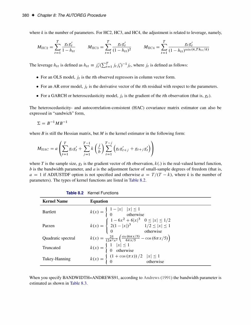
380 F Chapter 8: The AUTOREG Procedure
where k is the number of parameters. For HC2, HC3, and HC4, the adjustment is related to leverage, namely,
MHC2 D
TXtD1
gtg0t
1 � ht tMHC3 D
TXtD1
gtg0t
.1 � ht t /2MHC4 D
TXtD1
gtg0t
.1 � ht t /min .4;T htt=k/
The leverage ht t is defined as ht t � j 0t .PTtD1 jtj
0t /�1jt , where jt is defined as follows:
� For an OLS model, jt is the tth observed regressors in column vector form.
� For an AR error model, jt is the derivative vector of the tth residual with respect to the parameters.
� For a GARCH or heteroscedasticity model, jt is the gradient of the tth observation (that is, gt ).
The heteroscedasticity- and autocorrelation-consistent (HAC) covariance matrix estimator can also beexpressed in “sandwich” form,
† D B�1MB�1
where B is still the Hessian matrix, but M is the kernel estimator in the following form:
MHAC D a
0@ TXtD1
gtg0t C
T�1XjD1
k
�j
b
� T�jXtD1
�gtg0tCj C gtCjg
0t
�1Awhere T is the sample size, gt is the gradient vector of tth observation, k.:/ is the real-valued kernel function,b is the bandwidth parameter, and a is the adjustment factor of small-sample degrees of freedom (that is,a D 1 if ADJUSTDF option is not specified and otherwise a D T=.T � k/, where k is the number ofparameters). The types of kernel functions are listed in Table 8.2.
Table 8.2 Kernel Functions
Kernel Name Equation
Bartlett k.x/ D
�1 � jxj jxj � 1
0 otherwise
Parzen k.x/ D
8<:1 � 6x2 C 6jxj3 0 � jxj � 1=2
2.1 � jxj/3 1=2 � jxj � 1
0 otherwise
Quadratic spectral k.x/ D 2512�2x2
�sin .6�x=5/6�x=5
� cos .6�x=5/�
Truncated k.x/ D
�1 jxj � 1
0 otherwise
Tukey-Hanning k.x/ D
�.1C cos .�x// =2 jxj � 10 otherwise
When you specify BANDWIDTH=ANDREWS91, according to Andrews (1991) the bandwidth parameter isestimated as shown in Table 8.3.
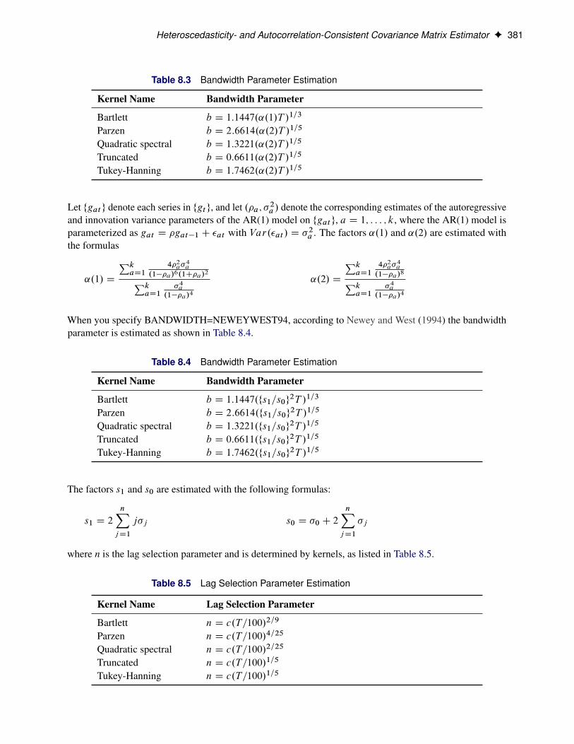
Heteroscedasticity- and Autocorrelation-Consistent Covariance Matrix Estimator F 381
Table 8.3 Bandwidth Parameter Estimation
Kernel Name Bandwidth Parameter
Bartlett b D 1:1447.˛.1/T /1=3
Parzen b D 2:6614.˛.2/T /1=5
Quadratic spectral b D 1:3221.˛.2/T /1=5
Truncated b D 0:6611.˛.2/T /1=5
Tukey-Hanning b D 1:7462.˛.2/T /1=5
Let fgatg denote each series in fgtg, and let .�a; �2a / denote the corresponding estimates of the autoregressiveand innovation variance parameters of the AR(1) model on fgatg, a D 1; : : : ; k, where the AR(1) model isparameterized as gat D �gat�1 C �at with Var.�at / D �2a . The factors ˛.1/ and ˛.2/ are estimated withthe formulas
˛.1/ D
PkaD1
4�2a�
4a
.1��a/6.1C�a/2PkaD1
�4a
.1��a/4
˛.2/ D
PkaD1
4�2a�
4a
.1��a/8PkaD1
�4a
.1��a/4
When you specify BANDWIDTH=NEWEYWEST94, according to Newey and West (1994) the bandwidthparameter is estimated as shown in Table 8.4.
Table 8.4 Bandwidth Parameter Estimation
Kernel Name Bandwidth Parameter
Bartlett b D 1:1447.fs1=s0g2T /1=3
Parzen b D 2:6614.fs1=s0g2T /1=5
Quadratic spectral b D 1:3221.fs1=s0g2T /1=5
Truncated b D 0:6611.fs1=s0g2T /1=5
Tukey-Hanning b D 1:7462.fs1=s0g2T /1=5
The factors s1 and s0 are estimated with the following formulas:
s1 D 2
nXjD1
j�j s0 D �0 C 2
nXjD1
�j
where n is the lag selection parameter and is determined by kernels, as listed in Table 8.5.
Table 8.5 Lag Selection Parameter Estimation
Kernel Name Lag Selection Parameter
Bartlett n D c.T=100/2=9
Parzen n D c.T=100/4=25
Quadratic spectral n D c.T=100/2=25
Truncated n D c.T=100/1=5
Tukey-Hanning n D c.T=100/1=5

382 F Chapter 8: The AUTOREG Procedure
The factor c in Table 8.5 is specified by the C= option; by default it is 12.
The factor �j is estimated with the equation
�j D T�1
TXtDjC1
0@ kXaDi
gat
kXaDi
gat�j
1A; j D 0; : : : ; nwhere i is 1 if the NOINT option in the MODEL statement is specified (otherwise, it is 2), and gat is thesame as in the Andrews method.
If you specify BANDWIDTH=SAMPLESIZE, the bandwidth parameter is estimated with the equation
b D
�b T r C cc if BANDWIDTH=SAMPLESIZE(INT) option is specified T r C c otherwise
where T is the sample size; bxc is the largest integer less than or equal to x; and , r, and c are valuesspecified by the BANDWIDTH=SAMPLESIZE(GAMMA=, RATE=, CONSTANT=) options, respectively.
If you specify the PREWHITENING option, gt is prewhitened by the VAR(1) model,
gt D Agt�1 C wt
Then M is calculated by
MHAC D a.I � A/�1
0@ TXtD1
wtw0t C
T�1XjD1
k
�j
b
� T�jXtD1
�wtw
0tCj C wtCjw
0t
�1A�.I � A/�1�0The bandwidth calculation is also based on the prewhitened series wt .
Goodness-of-Fit Measures and Information CriteriaThis section discusses various goodness-of-fit statistics produced by the AUTOREG procedure.
Total R-Square Statistic
The total R-square statistic (Total Rsq) is computed as
R2tot D 1 �SSESST
where SST is the sum of squares for the original response variable corrected for the mean and SSE is thefinal error sum of squares. The Total Rsq is a measure of how well the next value can be predicted using thestructural part of the model and the past values of the residuals. If the NOINT option is specified, SST is theuncorrected sum of squares.
Transformed Regression R-Square Statistic
The transformed regression R-square statistic is computed as
R2tr D 1 �TSSETSST
Goodness-of-Fit Measures and Information Criteria F 383
where TSST is the total sum of squares of the transformed response variable corrected for the transformedintercept, and TSSE is the error sum of squares for this transformed regression problem. If the NOINToption is requested, no correction for the transformed intercept is made. The transformed regression R-squarestatistic is a measure of the fit of the structural part of the model after transforming for the autocorrelationand is the R-square for the transformed regression.
Mean Absolute Error and Mean Absolute Percentage Error
The mean absolute error (MAE) is computed as
MAE D1
T
TXtD1
jet j
where et are the estimated model residuals and T is the number of observations.
The mean absolute percentage error (MAPE) is computed as
MAPE D1
T 0
TXtD1
ıyt¤0
jet j
jyt j
where et are the estimated model residuals, yt are the original response variable observations, ıyt¤0 D 1 ifyt ¤ 0, ıyt¤0 jet=yt j D 0 if yt D 0, and T 0 is the number of nonzero original response variable observations.
Calculation of Recursive Residuals and CUSUM Statistics
The recursive residuals wt are computed as
wt Detpvt
et D yt � x0tˇ.t/
ˇ.t/ D
"t�1XiD1
xix0i
#�1 t�1XiD1
xiyi
!
vt D 1C x0t
"t�1XiD1
xix0i
#�1xt
Note that the first ˇ.t/ can be computed for t D p C 1, where p is the number of regression coefficients. Asa result, first p recursive residuals are not defined. Note also that the forecast error variance of et is the scalarmultiple of vt such that V.et / D �2vt .
The CUSUM and CUSUMSQ statistics are computed using the preceding recursive residuals,
CUSUMt D
tXiDkC1
wi
�w
CUSUMSQt DPtiDkC1w
2iPT
iDkC1w2i

384 F Chapter 8: The AUTOREG Procedure
where wi are the recursive residuals,
�w D
sPTiDkC1 .wi � Ow/
2
.T � k � 1/
Ow D1
T � k
TXiDkC1
wi
and k is the number of regressors.
The CUSUM statistics can be used to test for misspecification of the model. The upper and lower criticalvalues for CUSUMt are
˙a
"p
T � k C 2.t � k/
.T � k/12
#
where a = 1.143 for a significance level 0.01, 0.948 for 0.05, and 0.850 for 0.10. These critical values areoutput by the CUSUMLB= and CUSUMUB= options for the significance level specified by the ALPHACSM=option.
The upper and lower critical values of CUSUMSQt are given by
˙aC.t � k/
T � k
where the value of a is obtained from the table by Durbin (1969) if the 12.T � k/ � 1 � 60. Edgerton and
Wells (1994) provided the method of obtaining the value of a for large samples.
These critical values are output by the CUSUMSQLB= and CUSUMSQUB= options for the significancelevel specified by the ALPHACSM= option.
Information Criteria AIC, AICC, SBC, and HQC
Akaike’s information criterion (AIC), the corrected Akaike’s information criterion (AICC), Schwarz’sBayesian information criterion (SBC), and the Hannan-Quinn information criterion (HQC) are computed asfollows:
AIC D �2ln.L/C 2k
AICC D AICC 2k.k C 1/
N � k � 1
SBC D �2ln.L/C ln.N /kHQC D �2ln.L/C 2ln.ln.N //k
In these formulas, L is the value of the likelihood function evaluated at the parameter estimates, N is thenumber of observations, and k is the number of estimated parameters. For more information, see Judge et al.(1985), Hurvich and Tsai (1989), Schwarz (1978) and Hannan and Quinn (1979).
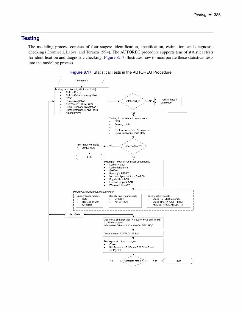
Testing F 385
TestingThe modeling process consists of four stages: identification, specification, estimation, and diagnosticchecking (Cromwell, Labys, and Terraza 1994). The AUTOREG procedure supports tens of statistical testsfor identification and diagnostic checking. Figure 8.17 illustrates how to incorporate these statistical testsinto the modeling process.
Figure 8.17 Statistical Tests in the AUTOREG Procedure
386 F Chapter 8: The AUTOREG Procedure
Testing for Stationarity
Most of the theories of time series require stationarity; therefore, it is critical to determine whether a timeseries is stationary. Two nonstationary time series are fractionally integrated time series and autoregressiveseries with random coefficients. However, more often some time series are nonstationary due to an upwardtrend over time. The trend can be captured by either of the following two models.
� The difference stationary process
.1 � L/yt D ı C .L/�t
where L is the lag operator, .1/ ¤ 0, and �t is a white noise sequence with mean zero and variance�2. Hamilton (1994) also refers to this model the unit root process.
� The trend stationary process
yt D ˛ C ıt C .L/�t
When a process has a unit root, it is said to be integrated of order one or I(1). An I(1) process is stationaryafter differencing once. The trend stationary process and difference stationary process require differenttreatment to transform the process into stationary one for analysis. Therefore, it is important to distinguishthe two processes. Bhargava (1986) nested the two processes into the following general model:
yt D 0 C 1t C ˛.yt�1 � 0 � 1.t � 1//C .L/�t
However, a difficulty is that the right-hand side is nonlinear in the parameters. Therefore, it is convenient touse a different parameterization:
yt D ˇ0 C ˇ1t C ˛yt�1 C .L/�t
The test of null hypothesis that ˛ D 1 against the one-sided alternative of ˛ < 1 is called a unit root test.
Dickey-Fuller unit root tests are based on regression models similar to the previous model,
yt D ˇ0 C ˇ1t C ˛yt�1 C �t
where �t is assumed to be white noise. The t statistic of the coefficient ˛ does not follow the normaldistribution asymptotically. Instead, its distribution can be derived using the functional central limit theorem.Three types of regression models including the preceding one are considered by the Dickey-Fuller test. Thedeterministic terms that are included in the other two types of regressions are either null or constant only.
An assumption in the Dickey-Fuller unit root test is that it requires the errors in the autoregressive model tobe white noise, which is often not true. There are two popular ways to account for general serial correlationbetween the errors. One is the augmented Dickey-Fuller (ADF) test, which uses the lagged difference in theregression model. This was originally proposed by Dickey and Fuller (1979) and later studied by Said andDickey (1984) and Phillips and Perron (1988). Another method is proposed by Phillips and Perron (1988);it is called Phillips-Perron (PP) test. The tests adopt the original Dickey-Fuller regression with intercept,but modify the test statistics to take account of the serial correlation and heteroscedasticity. It is callednonparametric because no specific form of the serial correlation of the errors is assumed.
A problem of the augmented Dickey-Fuller and Phillips-Perron unit root tests is that they are subject to sizedistortion and low power. It is reported in Schwert (1989) that the size distortion is significant when the
Testing F 387
series contains a large moving average (MA) parameter. DeJong et al. (1992) find that the ADF has poweraround one third and PP test has power less than 0.1 against the trend stationary alternative, in some commonsettings. Among some more recent unit root tests that improve upon the size distortion and the low power arethe tests described by Elliott, Rothenberg, and Stock (1996) and Ng and Perron (2001). These tests involvea step of detrending before constructing the test statistics and are demonstrated to perform better than thetraditional ADF and PP tests.
Most testing procedures specify the unit root processes as the null hypothesis. Tests of the null hypothesis ofstationarity have also been studied, among which Kwiatkowski et al. (1992) is very popular.
Economic theories often dictate that a group of economic time series are linked together by some long-runequilibrium relationship. Statistically, this phenomenon can be modeled by cointegration. When severalnonstationary processes zt D .z1t ; : : : ; zkt /0 are cointegrated, there exists a .k�1/ cointegrating vector csuch that c0zt is stationary and c is a nonzero vector. One way to test the relationship of cointegration is theresidual based cointegration test, which assumes the regression model
yt D ˇ1 C x0tˇ C ut
where yt D z1t , xt D .z2t ; : : : ; zkt /0, and ˇ D .ˇ2; : : : ; ˇk/0. The OLS residuals from the regression modelare used to test for the null hypothesis of no cointegration. Engle and Granger (1987) suggest using ADF onthe residuals while Phillips and Ouliaris (1990) study the tests using PP and other related test statistics.
Augmented Dickey-Fuller Unit Root and Engle-Granger Cointegration TestingCommon unit root tests have the null hypothesis that there is an autoregressive unit root H0 W ˛ D 1, and thealternative is Ha W j˛j < 1, where ˛ is the autoregressive coefficient of the time series
yt D ˛yt�1 C �t
This is referred to as the zero mean model. The standard Dickey-Fuller (DF) test assumes that errors �t arewhite noise. There are two other types of regression models that include a constant or a time trend as follows:
yt D �C ˛yt�1 C �t
yt D �C ˇt C ˛yt�1 C �t
These two models are referred to as the constant mean model and the trend model, respectively. The constantmean model includes a constant mean � of the time series. However, the interpretation of � depends on thestationarity in the following sense: the mean in the stationary case when ˛ < 1 is the trend in the integratedcase when ˛ D 1. Therefore, the null hypothesis should be the joint hypothesis that ˛ D 1 and � D 0.However, for the unit root tests, the test statistics are concerned with the null hypothesis of ˛ D 1. The jointnull hypothesis is not commonly used. This issue is addressed in Bhargava (1986) with a different nestingmodel.
There are two types of test statistics. The conventional t ratio is
DF� DO � 1
sd. O /
and the second test statistic, called �-test, is
T . O � 1/
388 F Chapter 8: The AUTOREG Procedure
For the zero mean model, the asymptotic distributions of the Dickey-Fuller test statistics are
T . O � 1/)
�Z 1
0
W.r/dW.r/
��Z 1
0
W.r/2dr
��1DF� )
�Z 1
0
W.r/dW.r/
��Z 1
0
W.r/2dr
��1=2For the constant mean model, the asymptotic distributions are
T . O � 1/)
�ŒW.1/2 � 1�=2 �W.1/
Z 1
0
W.r/dr
� Z 1
0
W.r/2dr �
�Z 1
0
W.r/dr
�2!�1
DF� )
�ŒW.1/2 � 1�=2 �W.1/
Z 1
0
W.r/dr
� Z 1
0
W.r/2dr �
�Z 1
0
W.r/dr
�2!�1=2
For the trend model, the asymptotic distributions are
T . O � 1/)
�W.r/dW C 12
�Z 1
0
rW.r/dr �1
2
Z 1
0
W.r/dr
��Z 1
0
W.r/dr �1
2W.1/
��W.1/
Z 1
0
W.r/dr
�D�1
DF� )
�W.r/dW C 12
�Z 1
0
rW.r/dr �1
2
Z 1
0
W.r/dr
��Z 1
0
W.r/dr �1
2W.1/
��W.1/
Z 1
0
W.r/dr
�D1=2
where
D D
Z 1
0
W.r/2dr � 12
�Z 1
0
r.W.r/dr
�2C 12
Z 1
0
W.r/dr
Z 1
0
rW.r/dr � 4
�Z 1
0
W.r/dr
�2One problem of the Dickey-Fuller and similar tests that employ three types of regressions is the difficulty inthe specification of the deterministic trends. Campbell and Perron (1991) claimed that “the proper handlingof deterministic trends is a vital prerequisite for dealing with unit roots.” However, the “proper handling”is not obvious since the distribution theory of the relevant statistics about the deterministic trends is notavailable. Hayashi (2000) suggests using the constant mean model when you think there is no trend, andusing the trend model when you think otherwise. However, no formal procedure is provided.
The null hypothesis of the Dickey-Fuller test is a random walk, possibly with drift. The differenced process isnot serially correlated under the null of I(1). There is a great need for the generalization of this specification.The augmented Dickey-Fuller (ADF) test, originally proposed in Dickey and Fuller (1979), adjusts for theserial correlation in the time series by adding lagged first differences to the autoregressive model,
�yt D �C ıt C ˛yt�1 C
pXjD1
˛j�yt�j C �t

Testing F 389
where the deterministic terms ıt and � can be absent for the models without drift or linear trend. Aspreviously, there are two types of test statistics. One is the OLS t value
O
sd. O /
and the other is given by
T O
1 � O1 � � � � � Op
The asymptotic distributions of the test statistics are the same as those of the standard Dickey-Fuller teststatistics.
Nonstationary multivariate time series can be tested for cointegration, which means that a linear combinationof these time series is stationary. Formally, denote the series by zt D .z1t ; : : : ; zkt /0. The null hypothesisof cointegration is that there exists a vector c such that c0zt is stationary. Residual-based cointegration testswere studied in Engle and Granger (1987) and Phillips and Ouliaris (1990). The latter are described in thenext subsection. The first step regression is
yt D x0tˇ C ut
where yt D z1t , xt D .z2t ; : : : ; zkt /0, and ˇ D .ˇ2; : : : ; ˇk/0. This regression can also include an interceptor an intercept with a linear trend. The residuals are used to test for the existence of an autoregressive unitroot. Engle and Granger (1987) proposed augmented Dickey-Fuller type regression without an intercepton the residuals to test the unit root. When the first step OLS does not include an intercept, the asymptoticdistribution of the ADF test statistic DF� is given by
DF� H)
Z 1
0
Q.r/
.R 10 Q
2/1=2dS
Q.r/ D W1.r/ �
Z 1
0
W1W02
�Z 1
0
W2W02
��1W2.r/
S.r/ DQ.r/
.�0�/1=2
�0 D
1;�
Z 1
0
W1W02
�Z 1
0
W2W02
��1!
where W.r/ is a k vector standard Brownian motion and
W.r/ D�W1.r/;W2.r/
�is a partition such that W1.r/ is a scalar and W2.r/ is k � 1 dimensional. The asymptotic distributions of thetest statistics in the other two cases have the same form as the preceding formula. If the first step regressionincludes an intercept, thenW.r/ is replaced by the de-meaned Brownian motionW .r/ D W.r/�
R 10 W.r/dr .
If the first step regression includes a time trend, thenW.r/ is replaced by the detrended Brownian motion. Thecritical values of the asymptotic distributions are tabulated in Phillips and Ouliaris (1990) and MacKinnon(1991).

390 F Chapter 8: The AUTOREG Procedure
The residual based cointegration tests have a major shortcoming. Different choices of the dependent variablein the first step OLS might produce contradictory results. This can be explained theoretically. If the dependentvariable is in the cointegration relationship, then the test is consistent against the alternative that there iscointegration. On the other hand, if the dependent variable is not in the cointegration system, the OLSresidual yt � x0tˇ do not converge to a stationary process. Changing the dependent variable is more likely toproduce conflicting results in finite samples.
Phillips-Perron Unit Root and Cointegration TestingBesides the ADF test, there is another popular unit root test that is valid under general serial correlation andheteroscedasticity, developed by Phillips (1987) and Phillips and Perron (1988). The tests are constructedusing the AR(1) type regressions, unlike ADF tests, with corrected estimation of the long run variance of�yt . In the case without intercept, consider the driftless random walk process
yt D yt�1 C ut
where the disturbances might be serially correlated with possible heteroscedasticity. Phillips and Perron(1988) proposed the unit root test of the OLS regression model,
yt D �yt�1 C ut
Denote the OLS residual by Out . The asymptotic variance of 1TPTtD1 Ou
2t can be estimated by using the
truncation lag l,
O� D
lXjD0
�j Œ1 � j=.l C 1/� O j
where �0 D 1, �j D 2 for j > 0, and O j D 1TPTtDjC1 Out Out�j . This is a consistent estimator suggested by
Newey and West (1987).
The variance of ut can be estimated by s2 D 1T�k
PTtD1 Ou
2t . Let O�2 be the variance estimate of the OLS
estimator O�. Then the Phillips-Perron OZ� test (zero mean case) is written
OZ� D T . O� � 1/ �1
2T 2O�2. O� � O 0/=s
2
The OZ� statistic is just the ordinary Dickey-Fuller OZ˛ statistic with a correction term that accounts for theserial correlation. The correction term goes to zero asymptotically if there is no serial correlation.
Note that P. O� < 1/�0:68 as T!1, which shows that the limiting distribution is skewed to the left.
Let �� be the � statistic for O�. The Phillips-Perron OZt (defined here as OZ� ) test is written
OZ� D . O 0= O�/1=2t O� �1
2T O�. O� � O 0/=.s O�1=2/
To incorporate a constant intercept, the regression model yt D �C �yt�1 C ut is used (single mean case)and null hypothesis the series is a driftless random walk with nonzero unconditional mean. To incorporatea time trend, we used the regression model yt D �C ıt C �yt�1 C ut and under the null the series is arandom walk with drift.
Testing F 391
The limiting distributions of the test statistics for the zero mean case are
OZ� )12fB.1/2 � 1gR 10 ŒB.s/�2ds
OZ� )12fŒB.1/�2 � 1g
fR 10 ŒB.x/�2dxg1=2
where B(�) is a standard Brownian motion.
The limiting distributions of the test statistics for the intercept case are
OZ� )
12fŒB.1/�2 � 1g � B.1/
R 10 B.x/dxR 1
0 ŒB.x/�2dx �hR 10 B.x/dx
i2OZ� )
12fŒB.1/�2 � 1g � B.1/
R 10 B.x/dx
fR 10 ŒB.x/�2dx �
hR 10 B.x/dx
i2g1=2
Finally, the limiting distributions of the test statistics for the trend case are can be derived as
�0 c 0
�V �1
264 B.1/�B.1/2 � 1
�=2
B.1/ �R 10 B.x/dx
375where c D 1 for OZ� and c D 1p
Qfor OZ� ,
V D
264 1R 10 B.x/dx 1=2R 1
0 B.x/dxR 10 B.x/2dx
R 10 xB.x/dx
1=2R 10 xB.x/dx 1=3
375Q D
�0 c 0
�V �1
�0 c 0
�TThe finite sample performance of the PP test is not satisfactory (see Hayashi 2000).
When several variables zt D .z1t ; : : : ; zkt /0 are cointegrated, there exists a .k�1/ cointegrating vector c suchthat c0zt is stationary and c is a nonzero vector. The residual based cointegration test assumes the followingregression model,
yt D ˇ1 C x0tˇ C ut
where yt D z1t , xt D .z2t ; : : : ; zkt /0, and ˇ D .ˇ2; : : : ; ˇk/0. You can estimate the consistent cointegratingvector by using OLS if all variables are difference stationary—that is, I(1). The estimated cointegratingvector is Oc D .1;� O2; : : : ;� Ok/0. The Phillips-Ouliaris test is computed using the OLS residuals fromthe preceding regression model, and it uses the PP unit root tests OZ� and OZ� developed in Phillips (1987),although in Phillips and Ouliaris (1990) the asymptotic distributions of some other leading unit root tests arealso derived. The null hypothesis is no cointegration.
You need to refer to the tables by Phillips and Ouliaris (1990) to obtain the p-value of the cointegration test.Before you apply the cointegration test, you might want to perform the unit root test for each variable (seethe option STATIONARITY=).
As in the Engle-Granger cointegration tests, the Phillips-Ouliaris test can give conflicting results for differentchoices of the regressand. There are other cointegration tests that are invariant to the order of the variables,including Johansen (1988), Johansen (1991), Stock and Watson (1988).
392 F Chapter 8: The AUTOREG Procedure
ERS and Ng-Perron Unit Root TestsAs mentioned earlier, ADF and PP both suffer severe size distortion and low power. There is a class of newertests that improve both size and power. These are sometimes called efficient unit root tests, and among themtests by Elliott, Rothenberg, and Stock (1996) and Ng and Perron (2001) are prominent.
Elliott, Rothenberg, and Stock (1996) consider the data generating process
yt D ˇ0zt C ut
ut D ˛ut�1 C vt ; t D 1; : : : ; T
where fztg is either f1g or f.1; t/g and fvtg is an unobserved stationary zero-mean process with positivespectral density at zero frequency. The null hypothesis is H0 W ˛ D 1, and the alternative is Ha W j˛j < 1.The key idea of Elliott, Rothenberg, and Stock (1996) is to study the asymptotic power and asymptotic powerenvelope of some new tests. Asymptotic power is defined with a sequence of local alternatives. For a fixedalternative hypothesis, the power of a test usually goes to one when sample size goes to infinity; however,this says nothing about the finite sample performance. On the other hand, when the data generating processunder the alternative moves closer to the null hypothesis as the sample size increases, the power does notnecessarily converge to one. The local-to-unity alternatives in ERS are
˛ D 1Cc
T
and the power against the local alternatives has a limit as T goes to infinity, which is called asymptotic power.This value is strictly between 0 and 1. Asymptotic power indicates the adequacy of a test to distinguish smalldeviations from the null hypothesis.
Define
y˛ D .y1; .1 � ˛L/y2; : : : ; .1 � ˛L/yT /
z˛ D .z1; .1 � ˛L/z2; : : : ; .1 � ˛L/zT /
Let S.˛/ be the sum of squared residuals from a least squares regression of y˛ on z˛ . Then the point optimaltest against the local alternative N D 1C Nc=T has the form
PGLST DS. N / � NS.1/
O!2
where O!2 is an estimator for !2 DP1kD�1Evtvt�k . The autoregressive (AR) estimator is used for O!2
(Elliott, Rothenberg, and Stock 1996, equations 13 and 14),
O!2 DO�2�
.1 �PpiD1 Oai /
2
where O�2� and Oai are OLS estimates from the regression
�yt D a0yt�1 C
pXiD1
ai�yt�i C apC1 C �t
where p is selected according to the Schwarz Bayesian information criterion. The test rejects the null whenPT is small. The asymptotic power function for the point optimal test that is constructed with Nc under localalternatives with c is denoted by �.c; Nc/. Then the power envelope is �.c; c/ because the test formed with Nc
Testing F 393
is the most powerful against the alternative c D Nc. In other words, the asymptotic function �.c; Nc/ is alwaysbelow the power envelope �.c/ except that at one point, c D Nc, they are tangent. Elliott, Rothenberg, andStock (1996) show that choosing some specific values for Nc can cause the asymptotic power function �.c; Nc/of the point optimal test to be very close to the power envelope. The optimal Nc is �7 when zt D 1, and �13:5when zt D .1; t/0. This choice of Nc corresponds to the tangent point where � D 0:5. This is also true of theDF-GLS test.
Elliott, Rothenberg, and Stock (1996) also propose the DF-GLS test, given by the t statistic for testing 0 D 0in the regression
�ydt D 0ydt�1 C
pXjD1
j�ydt�j C �tp
where ydt is obtained in a first step detrending
ydt D yt �O0N zt
and O N is least squares regression coefficient of y˛ on z˛. Regarding the lag length selection, Elliott,Rothenberg, and Stock (1996) favor the Schwarz Bayesian information criterion. The optimal selection of thelag length p and the estimation of !2 is further discussed in Ng and Perron (2001). The lag length is selectedfrom the interval Œ0; pmax� for some fixed pmax by using the modified Akaike’s information criterion,
MAIC.p/ D log. O�2p/C2.�T .p/C p/
T � pmax
where �T .p/ D . O�2p/�1 O 20
PT�1tDpmaxC1
.ydt /2 and O�2p D .T � pmax � 1/
�1PT�1tDpmaxC1
O�2tp . For fixed laglength p, an estimate of !2 is given by
O!2 D.T � 1 � p/�1
PTtDpC2 O�
2tp�
1 �PpjD1O j
�2DF-GLS is indeed a superior unit root test, according to Stock (1994), Schwert (1989), and Elliott, Rothenberg,and Stock (1996). In terms of the size of the test, DF-GLS is almost as good as the ADF t test DF� and betterthan the PP OZ� and OZ� test. In addition, the power of the DF-GLS test is greater than that of both the ADF ttest and the �-test.
Ng and Perron (2001) also apply GLS detrending to obtain the following M-tests:
MZ˛ D ..T � 1/�1.ydT /
2� O!2/
2.T � 1/�2
T�1XtD1
.ydt /2
!�1
MSB D
PT�1tD1 .y
dt /2
.T � 1/2 O!2
!1=2MZt DMZ˛ �MSB
The first one is a modified version of the Phillips-Perron Z� test,
MZ� D Z� CT
2. O � 1/2
394 F Chapter 8: The AUTOREG Procedure
where the detrended data fydt g is used. The second is a modified Bhargava (1986) R1 test statistic. The thirdcan be perceived as a modified Phillips-Perron Z� statistic because of the relationship Z� DMSB � Z�.
The modified point optimal tests that use the GLS detrended data are
MPGLST DNc2.T�1/�2
PT�1tD1 .y
dt /
2�Nc.T�1/�1.ydT /
2
O!2 for zt D 1
MPGLST DNc2.T�1/�2
PT�1tD1 .y
dt /
2C.1�Nc/.T�1/�1.ydT /
2
O!2 for zt D .1; t/
The DF-GLS test and the MZt test have the same limiting distribution:
DF-GLS �MZt ) 0:5 .Jc.1/2�1/�R 1
0 Jc.r/2dr�1=2 for zt D 1
DF-GLS �MZt ) 0:5.Vc; Nc.1/
2�1/�R 10 Vc; Nc.r/2dr
�1=2 for zt D .1; t/
The point optimal test and the modified point optimal test have the same limiting distribution,
PGLST �MPGLST ) Nc2R 10 Jc.r/
2dr � NcJc.1/2 for zt D 1
PGLST �MPGLST ) Nc2R 10 Vc; Nc.r/
2dr C .1 � Nc/Vc; Nc.1/2 for zt D .1; t/
whereW.r/ is a standard Brownian motion and Jc.r/ is an Ornstein-Uhlenbeck process defined by dJc.r/ DcJc.r/dr C dW.r/ with Jc.0/ D 0, Vc; Nc.r/ D Jc.r/ � r
h�Jc.1/C 3.1 � �/
R 10 sJc.s/ds
i, and � D
.1 � Nc/=.1 � Nc C Nc2=3/.
Overall, the M-tests have the smallest size distortion, with the ADF t test having the next smallest. TheADF �-test, OZ�, and OZ� have the largest size distortion. In addition, the power of the DF-GLS and M-tests isgreater than that of the ADF t test and �-test. The ADF OZ� has more severe size distortion than the ADF OZ� ,but it has more power for a fixed lag length.
Kwiatkowski, Phillips, Schmidt, and Shin (KPSS) Unit Root Test and Shin Cointegration TestThere are fewer tests available for the null hypothesis of trend stationarity I(0). The main reason is thedifficulty of theoretical development. The KPSS test was introduced in Kwiatkowski et al. (1992) to testthe null hypothesis that an observable series is stationary around a deterministic trend. For consistency, thenotation used here differs from the notation in the original paper. The setup of the problem is as follows: it isassumed that the series is expressed as the sum of the deterministic trend, random walk rt , and stationaryerror ut ; that is,
yt D �C ıt C rt C ut
rt D rt�1 C et
where et �iid .0; �2e /, and an intercept � (in the original paper, the authors use r0 instead of �; here weassume r0 D 0.) The null hypothesis of trend stationarity is specified by H0 W �2e D 0, while the null of levelstationarity is the same as above with the model restriction ı D 0. Under the alternative that �2e ¤ 0, there isa random walk component in the observed series yt .
Testing F 395
Under stronger assumptions of normality and iid of ut and et , a one-sided LM test of the null that there is norandom walk (et D 0;8t ) can be constructed as follows:
bLM D1
T 2
TXtD1
S2ts2.l/
s2.l/ D1
T
TXtD1
Ou2t C2
T
lXsD1
w.s; l/
TXtDsC1
Out Out�s
St D
tX�D1
Ou�
Under the null hypothesis, Out can be estimated by ordinary least squares regression of yt on an interceptand the time trend. Following the original work of Kwiatkowski et al. (1992), under the null (�2e D 0), thebLM statistic converges asymptotically to three different distributions depending on whether the model istrend-stationary, level-stationary (ı D 0), or zero-mean stationary (ı D 0, � D 0). The trend-stationarymodel is denoted by subscript � and the level-stationary model is denoted by subscript �. The case when thereis no trend and zero intercept is denoted as 0. The last case, although rarely used in practice, is considered inHobijn, Franses, and Ooms (2004),
yt D ut W bLM 0D�!
Z 1
0
B2.r/dr
yt D �C ut W bLM�D�!
Z 1
0
V 2.r/dr
yt D �C ıt C ut W bLM �D�!
Z 1
0
V 22 .r/dr
with
V.r/ D B.r/ � rB.1/
V2.r/ D B.r/C .2r � 3r2/B.1/C .�6r C 6r2/
Z 1
0
B.s/ds
where B.r/ is a Brownian motion (Wiener process) andD�! is convergence in distribution. V.r/ is a standard
Brownian bridge, and V2.r/ is a second-level Brownian bridge.
Using the notation of Kwiatkowski et al. (1992), the bLM statistic is named as O�. This test depends on thecomputational method used to compute the long-run variance s.l/; that is, the window width l and the kerneltype w.�; �/. You can specify the kernel used in the test by using the KERNEL option:
� Newey-West/Bartlett (KERNEL=NW j BART) (this is the default)
w.s; l/ D 1 �s
l C 1
� quadratic spectral (KERNEL=QS)
w.s; l/ D Qw�sl
�D Qw.x/ D
25
12�2x2
�sin .6�x=5/6�x=5
� cos�6
5�x
��
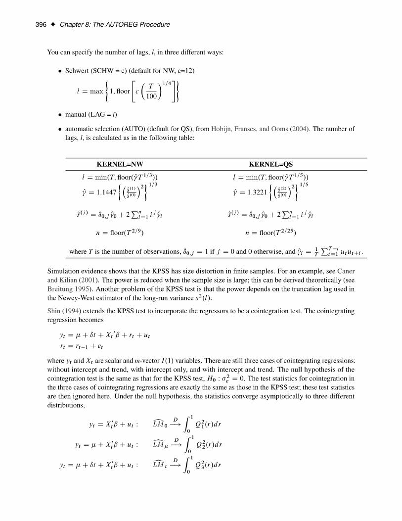
396 F Chapter 8: The AUTOREG Procedure
You can specify the number of lags, l, in three different ways:
� Schwert (SCHW = c) (default for NW, c=12)
l D max
(1;floor
"c
�T
100
�1=4#)
� manual (LAG = l)
� automatic selection (AUTO) (default for QS), from Hobijn, Franses, and Ooms (2004). The number oflags, l, is calculated as in the following table:
KERNEL=NW KERNEL=QS
l D min.T;floor. O T 1=3// l D min.T;floor. O T 1=5//
O D 1:1447
��Os.1/
Os.0/
�2�1=3O D 1:3221
��Os.2/
Os.0/
�2�1=5Os.j / D ı0;j O 0 C 2
PniD1 i
j O i Os.j / D ı0;j O 0 C 2PniD1 i
j O i
n D floor.T 2=9/ n D floor.T 2=25/
where T is the number of observations, ı0;j D 1 if j D 0 and 0 otherwise, and O i D 1T
PT�itD1 ututCi .
Simulation evidence shows that the KPSS has size distortion in finite samples. For an example, see Canerand Kilian (2001). The power is reduced when the sample size is large; this can be derived theoretically (seeBreitung 1995). Another problem of the KPSS test is that the power depends on the truncation lag used inthe Newey-West estimator of the long-run variance s2.l/.
Shin (1994) extends the KPSS test to incorporate the regressors to be a cointegration test. The cointegratingregression becomes
yt D �C ıt CXt0ˇ C rt C ut
rt D rt�1 C et
where yt andXt are scalar and m-vector I.1/ variables. There are still three cases of cointegrating regressions:without intercept and trend, with intercept only, and with intercept and trend. The null hypothesis of thecointegration test is the same as that for the KPSS test, H0 W �2e D 0. The test statistics for cointegration inthe three cases of cointegrating regressions are exactly the same as those in the KPSS test; these test statisticsare then ignored here. Under the null hypothesis, the statistics converge asymptotically to three differentdistributions,
yt D X0tˇ C ut W
bLM 0D�!
Z 1
0
Q21.r/dr
yt D �CX0tˇ C ut W
bLM�D�!
Z 1
0
Q22.r/dr
yt D �C ıt CX0tˇ C ut W
bLM �D�!
Z 1
0
Q23.r/dr
Testing F 397
with
Q1.r/ D B.r/ �
�Z r
0
Bm.x/dx
��Z 1
0
Bm.x/Bm0.x/dx
��1 �Z 1
0
Bm.x/dB.x/
�Q2.r/ D V.r/ �
�Z r
0
NBm.x/dx
��Z 1
0
NBm.x/NBm0.x/dx
��1 �Z 1
0
NBm.x/dB.x/
�Q3.r/ D V2.r/ �
�Z r
0
B�m.x/dx��Z 1
0
B�m.x/B�m0.x/dx
��1 �Z 1
0
B�m.x/dB.x/�
whereB.:/ and Bm.:/ are independent scalar and m-vector standard Brownian motion, andD�! is convergence
in distribution. V.r/ is a standard Brownian bridge, V2.r/ is a Brownian bridge of a second-level, NBm.r/ D
Bm.r/ �R 10 Bm.x/dx is an m-vector standard de-meaned Brownian motion, and B�m.r/ D Bm.r/C .6r �
4/R 10 Bm.x/dx C .�12r C 6/
R 10 xBm.x/dx is an m-vector standard de-meaned and detrended Brownian
motion.
The p-values that are reported for the KPSS test and Shin test are calculated via a Monte Carlo simulation ofthe limiting distributions, using a sample size of 2,000 and 1,000,000 replications.
Testing for Statistical Independence
Independence tests are widely used in model selection, residual analysis, and model diagnostics becausemodels are usually based on the assumption of independently distributed errors. If a given time series (forexample, a series of residuals) is independent, then no deterministic model is necessary for this completelyrandom process; otherwise, there must exist some relationship in the series to be addressed. In the followingsection, four independence tests are introduced: the BDS test, the runs test, the turning point test, and therank version of von Neumann ratio test.
BDS TestBrock, Dechert, and Scheinkman (1987) propose a test (BDS test) of independence based on the correlationdimension. Brock et al. (1996) show that the first-order asymptotic distribution of the test statistic isindependent of the estimation error provided that the parameters of the model under test can be estimatedpn-consistently. Hence, the BDS test can be used as a model selection tool and as a specification test.
Given the sample size T, the embedding dimension m, and the value of the radius r, the BDS statistic is
SBDS.T;m; r/ DpT �mC 1
cm;m;T .r/ � cm1;m;T .r/
�m;T .r/
398 F Chapter 8: The AUTOREG Procedure
where
cm;n;N .r/ D2
.N � nC 1/.N � n/
NXsDn
NXtDsC1
m�1YjD0
Ir.zs�j ; zt�j /
Ir.zs; zt / D
�1 if jzs � zt j < r0 otherwise
�2m;T .r/ D 4
0@km C 2m�1XjD1
km�j c2j C .m � 1/2c2m �m2kc2m�2
1Ac D c1;1;T .r/
k D kT .r/ D6
T .T � 1/.T � 2/
TXtD1
TXsDtC1
TXlDsC1
hr.zt ; zs; zl/
hr.zt ; zs; zl/ D1
3.Ir.zt ; zs/Ir.zs; zl/C Ir.zt ; zl/Ir.zl ; zs/C Ir.zs; zt /Ir.zt ; zl//
The statistic has a standard normal distribution if the sample size is large enough. For small sample size,the distribution can be approximately obtained through simulation. Kanzler (1999) has a comprehensivediscussion on the implementation and empirical performance of BDS test.
Runs Test and Turning Point TestThe runs test and turning point test are two widely used tests for independence (Cromwell, Labys, and Terraza1994).
The runs test needs several steps. First, convert the original time series into the sequence of signs, fCC ��� � � C � � �g, that is, map fztg into fsign.zt � zM /g where zM is the sample mean of zt and sign.x/ is“C” if x is nonnegative and “�” if x is negative. Second, count the number of runs, R, in the sequence. A runof a sequence is a maximal non-empty segment of the sequence that consists of adjacent equal elements. Forexample, the following sequence contains R D 8 runs:
CCC„ ƒ‚ …1
� � �„ƒ‚…1
CC„ƒ‚…1
��„ƒ‚…1
C„ƒ‚…1
�„ƒ‚…1
CCCCC„ ƒ‚ …1
��„ƒ‚…1
Third, count the number of pluses and minuses in the sequence and denote them as NC and N�, respectively.In the preceding example sequence, NC D 11 and N� D 8. Note that the sample size T D NC C N�.Finally, compute the statistic of runs test,
Sruns DR � �
�
where
� D2NCN�
TC 1
�2 D.� � 1/.� � 2/
T � 1
The statistic of the turning point test is defined as
STP D
PT�1tD2 TPt � 2.T � 2/=3p
.16T � 29/=90
Testing F 399
where the indicator function of the turning point TPt is 1 if zt > zt˙1 or zt < zt˙1 (that is, both the previousand next values are greater or less than the current value); otherwise, 0.
The statistics of both the runs test and the turning point test have the standard normal distribution under thenull hypothesis of independence.
Rank Version of the von Neumann Ratio TestBecause the runs test completely ignores the magnitudes of the observations, Bartels (1982) proposes a rankversion of the von Neumann ratio test for independence,
SRVN D
pT
2
PT�1tD1 .RtC1 �Rt /
2
.T .T 2 � 1/=12/� 2
!
where Rt is the rank of tth observation in the sequence of T observations. For large samples, the statisticfollows the standard normal distribution under the null hypothesis of independence. For small samples of sizebetween 11 and 100, the critical values that have been simulated would be more precise. For samples of sizeless than or equal to 10, the exact CDF of the statistic is available. Hence, the VNRRANK=(PVALUE=SIM)option is recommended for small samples whose size is no more than 100, although it might take longer toobtain the p-value than if you use the VNRRANK=(PVALUE=DIST) option.
Testing for Normality
Based on skewness and kurtosis, Jarque and Bera (1980) calculated the test statistic
TN D
�N
6b21 C
N
24.b2 � 3/
2
�where
b1 D
pNPNtD1 Ou
3t�PN
tD1 Ou2t
� 32
b2 DNPNtD1 Ou
4t�PN
tD1 Ou2t
�2The �2(2) distribution gives an approximation to the normality test TN .
When the GARCH model is estimated, the normality test is obtained using the standardized residualsOut D O�t=
pht . The normality test can be used to detect misspecification of the family of ARCH models.
Testing for Linear Dependence
Generalized Durbin-Watson TestsConsider the linear regression model
Y D Xˇ C �
where X is an N � k data matrix, ˇ is a k � 1 coefficient vector, and � is an N � 1 disturbance vector. Theerror term � is assumed to be generated by the jth-order autoregressive process �t D �t � 'j �t�j where

400 F Chapter 8: The AUTOREG Procedure
j'j j < 1, �t is a sequence of independent normal error terms with mean 0 and variance �2. Usually, theDurbin-Watson statistic is used to test the null hypothesis H0 W '1 D 0 against H1 W �'1 > 0. Vinod (1973)generalized the Durbin-Watson statistic,
dj D
PNtDjC1 . O�t � O�t�j /
2PNtD1 O�
2t
where O� are OLS residuals. Using the matrix notation,
dj DY0MA0jAjMY
Y0MY
where M D IN �X.X0X/�1X0 and Aj is a .N � j / �N matrix,
Aj D
26664�1 0 � � � 0 1 0 � � � 0
0 �1 0 � � � 0 1 0 � � �
::::::
::::::
::::::
::::::
0 � � � 0 �1 0 � � � 0 1
37775and there are j � 1 zeros between �1 and 1 in each row of matrix Aj .
The QR factorization of the design matrix X yields an N �N orthogonal matrix Q,
X D QR
where R is an N � k upper triangular matrix. There exists an N � .N � k/ submatrix of Q such thatQ1Q01 DM and Q01Q1 D IN�k . Consequently, the generalized Durbin-Watson statistic is stated as a ratio oftwo quadratic forms,
dj D
PnlD1 �jl�l
2PnlD1 �
2l
where �j1 : : : �jn are upper n eigenvalues of MA0jAjM and �l is a standard normal variate, andn D min.N � k;N � j /. These eigenvalues are obtained by a singular value decomposition of Q01A0j(Golub and Van Loan 1989; Savin and White 1978).
The marginal probability (or p-value) for dj given c0 is
Prob.PnlD1 �jl�
2lPn
lD1 �2l
< c0/ D Prob.qj < 0/
where
qj D
nXlD1
.�jl � c0/�2l
When the null hypothesis H0 W 'j D 0 holds, the quadratic form qj has the characteristic function
�j .t/ D
nYlD1
.1 � 2.�jl � c0/i t/�1=2
Testing F 401
The distribution function is uniquely determined by this characteristic function:
F.x/ D1
2C
1
2�
Z 10
eitx�j .�t / � e�itx�j .t/
i tdt
For example, to test H0 W '4 D 0 given '1 D '2 D '3 D 0 against H1 W �'4 > 0, the marginal probability(p-value) can be used,
F.0/ D1
2C
1
2�
Z 10
.�4.�t / � �4.t//
i tdt
where
�4.t/ D
nYlD1
.1 � 2.�4l � Od4/i t/�1=2
and Od4 is the calculated value of the fourth-order Durbin-Watson statistic.
In the Durbin-Watson test, the marginal probability indicates positive autocorrelation (�'j > 0) if it is lessthan the level of significance (˛), while you can conclude that a negative autocorrelation (�'j < 0) exists ifthe marginal probability based on the computed Durbin-Watson statistic is greater than 1 � ˛. Wallis (1972)presented tables for bounds tests of fourth-order autocorrelation, and Vinod (1973) has given tables for a5% significance level for orders two to four. Using the AUTOREG procedure, you can calculate the exactp-values for the general order of Durbin-Watson test statistics. Tests for the absence of autocorrelation oforder p can be performed sequentially; at the jth step, test H0 W 'j D 0 given '1 D � � � D 'j�1 D 0 against'j ¤ 0. However, the size of the sequential test is not known.
The Durbin-Watson statistic is computed from the OLS residuals, while that of the autoregressive error modeluses residuals that are the difference between the predicted values and the actual values. When you use theDurbin-Watson test from the residuals of the autoregressive error model, you must be aware that this testis only an approximation. See the section “Autoregressive Error Model” on page 368. If there are missingvalues, the Durbin-Watson statistic is computed using all the nonmissing values and ignoring the gaps causedby missing residuals. This does not affect the significance level of the resulting test, although the power ofthe test against certain alternatives may be adversely affected. Savin and White (1978) have examined theuse of the Durbin-Watson statistic with missing values.
The Durbin-Watson probability calculations have been enhanced to compute the p-value of the generalizedDurbin-Watson statistic for large sample sizes. Previously, the Durbin-Watson probabilities were onlycalculated for small sample sizes.
Consider the linear regression model
Y D Xˇ C u
ut C 'jut�j D �t ; t D 1; : : : ; N
where X is an N � k data matrix, ˇ is a k � 1 coefficient vector, u is an N � 1 disturbance vector, and �t is asequence of independent normal error terms with mean 0 and variance �2.
The generalized Durbin-Watson statistic is written as
DWj DOu0A0jAj Ou
Ou0 Ou
402 F Chapter 8: The AUTOREG Procedure
where Ou is a vector of OLS residuals and Aj is a .T � j / � T matrix. The generalized Durbin-Watsonstatistic DWj can be rewritten as
DWj DY0MA0jAjMY
Y0MYD�0.Q01A
0jAjQ1/�
�0�
where Q01Q1 D IT�k; Q01X D 0; and � D Q01u.
The marginal probability for the Durbin-Watson statistic is
Pr.DWj < c/ D Pr.h < 0/
where h D �0.Q01A0jAjQ1 � cI/�.
The p-value or the marginal probability for the generalized Durbin-Watson statistic is computed by numericalinversion of the characteristic function �.u/ of the quadratic form h D �0.Q01A
0jAjQ1�cI/�. The trapezoidal
rule approximation to the marginal probability Pr.h < 0/ is
Pr.h < 0/ D1
2�
KXkD0
Im��..k C 1
2/�/
��.k C 1
2/
C EI .�/C ET .K/
where Im Œ�.�/� is the imaginary part of the characteristic function, EI .�/ and ET .K/ are integration andtruncation errors, respectively. For numerical inversion of the characteristic function, see Davies (1973).
Ansley, Kohn, and Shively (1992) proposed a numerically efficient algorithm that requires O(N) operationsfor evaluation of the characteristic function �.u/. The characteristic function is denoted as
�.u/ DˇI � 2iu.Q01A
0jAjQ1 � cIN�k/
ˇ�1=2D jVj�1=2
ˇX0V�1X
ˇ�1=2 ˇX0X
ˇ1=2where V D .1C2iuc/I�2iuA0jAj and i D
p�1. By applying the Cholesky decomposition to the complex
matrix V, you can obtain the lower triangular matrix G that satisfies V D GG0. Therefore, the characteristicfunction can be evaluated in O(N) operations by using the formula
�.u/ D jGj�1ˇX�0X�
ˇ�1=2 ˇX0Xˇ1=2where X� D G�1X. For more information about evaluation of the characteristic function, see Ansley, Kohn,and Shively (1992).
Tests for Serial Correlation with Lagged Dependent VariablesWhen regressors contain lagged dependent variables, the Durbin-Watson statistic (d1) for the first-orderautocorrelation is biased toward 2 and has reduced power. Wallis (1972) shows that the bias in the Durbin-Watson statistic (d4) for the fourth-order autocorrelation is smaller than the bias in d1 in the presence of afirst-order lagged dependent variable. Durbin (1970) proposes two alternative statistics (Durbin h and t) thatare asymptotically equivalent. The h statistic is written as
h D O�
qN=.1 �N OV /

Testing F 403
where O� DPNtD2 O�t O�t�1=
PNtD1 O�
2t and OV is the least squares variance estimate for the coefficient of the
lagged dependent variable. Durbin’s t test consists of regressing the OLS residuals O�t on explanatory variablesand O�t�1 and testing the significance of the estimate for coefficient of O�t�1.
Inder (1984) shows that the Durbin-Watson test for the absence of first-order autocorrelation is generallymore powerful than the h test in finite samples. For information about the Durbin-Watson test in the presenceof lagged dependent variables, see Inder (1986) and King and Wu (1991).
Godfrey LM testThe GODFREY= option in the MODEL statement produces the Godfrey Lagrange multiplier test for seriallycorrelated residuals for each equation (Godfrey 1978b, a). r is the maximum autoregressive order, andspecifies that Godfrey’s tests be computed for lags 1 through r. The default number of lags is four.
Testing for Nonlinear Dependence: Ramsey’s Reset Test
Ramsey’s reset test is a misspecification test associated with the functional form of models to check whetherpower transforms need to be added to a model. The original linear model, henceforth called the restrictedmodel, is
yt D xtˇ C ut
To test for misspecification in the functional form, the unrestricted model is
yt D xtˇ C
pXjD2
�j Oyjt C ut
where Oyt is the predicted value from the linear model and p is the power of Oyt in the unrestricted modelequation starting from 2. The number of higher-ordered terms to be chosen depends on the discretion of theanalyst. The RESET option produces test results for p D 2, 3, and 4.
The reset test is an F statistic for testing H0 W �j D 0, for all j D 2; : : : ; p, against H1 W �j ¤ 0 for at leastone j D 2; : : : ; p in the unrestricted model and is computed as
F.p�1;n�k�pC1/ D.SSER � SSEU /=.p � 1/SSEU =.n � k � p C 1/
where SSER is the sum of squared errors due to the restricted model, SSEU is the sum of squared errors dueto the unrestricted model, n is the total number of observations, and k is the number of parameters in theoriginal linear model.
Ramsey’s test can be viewed as a linearity test that checks whether any nonlinear transformation of thespecified independent variables has been omitted, but it need not help in identifying a new relevant variableother than those already specified in the current model.
Testing for Nonlinear Dependence: Heteroscedasticity Tests
Portmanteau Q TestFor nonlinear time series models, the portmanteau test statistic based on squared residuals is used to test forindependence of the series (McLeod and Li 1983),
Q.q/ D N.N C 2/
qXiD1
r.i I O�2t /
.N � i/

404 F Chapter 8: The AUTOREG Procedure
where
r.i I O�2t / D
PNtDiC1 . O�
2t � O�
2/. O�2t�i � O�2/PN
tD1 . O�2t � O�
2/2
O�2 D1
N
NXtD1
O�2t
This Q statistic is used to test the nonlinear effects (for example, GARCH effects) present in the residuals. TheGARCH.p; q/ process can be considered as an ARMA.max.p; q/; p/ process. See the section “Predictingthe Conditional Variance” on page 411. Therefore, the Q statistic calculated from the squared residuals canbe used to identify the order of the GARCH process.
Engle’s Lagrange Multiplier Test for ARCH DisturbancesEngle (1982) proposed a Lagrange multiplier test for ARCH disturbances. The test statistic is asymptoticallyequivalent to the test used by Breusch and Pagan (1979). Engle’s Lagrange multiplier test for the qth orderARCH process is written
LM.q/ DNW0Z.Z0Z/�1Z0W
W0W
where
W D
O�21O�2� 1; : : : ;
O�2NO�2� 1
!0and
Z D
2666641 O�20 � � � O�2
�qC1:::
::::::
::::::
::::::
:::
1 O�2N�1 � � � O�2N�q
377775The presample values ( �20 , . . . , �2
�qC1) have been set to 0. Note that the LM.q/ tests might have differentfinite-sample properties depending on the presample values, though they are asymptotically equivalentregardless of the presample values.
Lee and King’s Test for ARCH DisturbancesEngle’s Lagrange multiplier test for ARCH disturbances is a two-sided test; that is, it ignores the inequalityconstraints for the coefficients in ARCH models. Lee and King (1993) propose a one-sided test and provethat the test is locally most mean powerful. Let "t ; t D 1; : : : ; T , denote the residuals to be tested. Lee andKing’s test checks
H0 W ˛i D 0; i D 1; : : : ; q
H1 W ˛i > 0; i D 1; : : : ; q
where ˛i ; i D 1; : : : ; q; are in the following ARCH(q) model:
"t Dphtet ; et i id.0; 1/
Testing F 405
ht D ˛0 C
qXiD1
˛i"2t�i
The statistic is written as
S D
PTtDqC1 .
"2t
h0� 1/
PqiD1 "
2t�i�
2PTtDqC1 .
PqiD1 "
2t�i /
2 �2.PT
tDqC1
Pq
iD1"2
t�i/2
T�q
�1=2
Wong and Li’s Test for ARCH DisturbancesWong and Li (1995) propose a rank portmanteau statistic to minimize the effect of the existence of outliers inthe test for ARCH disturbances. They first rank the squared residuals; that is, Rt D rank."2t /. Then theycalculate the rank portmanteau statistic
QR D
qXiD1
.ri � �i /2
�2i
where ri , �i , and �2i are defined as follows:
ri D
PTtDiC1 .Rt � .T C 1/=2/.Rt�i � .T C 1/=2/
T .T 2 � 1/=12
�i D �T � i
T .T � 1/
�2i D5T 4 � .5i C 9/T 3 C 9.i � 2/T 2 C 2i.5i C 8/T C 16i2
5.T � 1/2T 2.T C 1/
The Q, Engle’s LM, Lee and King’s, and Wong and Li’s statistics are computed from the OLS residuals, orresiduals if the NLAG= option is specified, assuming that disturbances are white noise. The Q, Engle’s LM,and Wong and Li’s statistics have an approximate �2
.q/distribution under the white-noise null hypothesis,
while the Lee and King’s statistic has a standard normal distribution under the white-noise null hypothesis.
Testing for Structural Change
Chow TestConsider the linear regression model
y D Xˇ C u
where the parameter vector ˇ contains k elements.
Split the observations for this model into two subsets at the break point specified by the CHOW= option, sothat
y D .y01; y02/0
X D .X01;X02/0
u D .u01; u02/0
406 F Chapter 8: The AUTOREG Procedure
Now consider the two linear regressions for the two subsets of the data modeled separately,
y1 D X1ˇ1 C u1
y2 D X2ˇ2 C u2
where the number of observations from the first set is n1 and the number of observations from the second setis n2.
The Chow test statistic is used to test the null hypothesisH0 W ˇ1 D ˇ2 conditional on the same error varianceV.u1/ D V.u2/. The Chow test is computed using three sums of square errors,
Fchow D. Ou0 Ou � Ou01 Ou1 � Ou
02 Ou2/=k
. Ou01 Ou1 C Ou02 Ou2/=.n1 C n2 � 2k/
where Ou is the regression residual vector from the full set model, Ou1 is the regression residual vector from thefirst set model, and Ou2 is the regression residual vector from the second set model. Under the null hypothesis,the Chow test statistic has an F distribution with k and .n1 C n2 � 2k/ degrees of freedom, where k is thenumber of elements in ˇ.
Chow (1960) suggested another test statistic that tests the hypothesis that the mean of prediction errors is 0.The predictive Chow test can also be used when n2 < k.
The PCHOW= option computes the predictive Chow test statistic
Fpchow D. Ou0 Ou � Ou01 Ou1/=n2Ou01 Ou1=.n1 � k/
The predictive Chow test has an F distribution with n2 and .n1 � k/ degrees of freedom.
Bai and Perron’s Multiple Structural Change TestsBai and Perron (1998) propose several kinds of multiple structural change tests: (1) the test of no break versusa fixed number of breaks (supF test), (2) the equal and unequal weighted versions of double maximum testsof no break versus an unknown number of breaks given some upper bound (UDmaxF test and WDmaxFtest), and (3) the test of l versus l C 1 breaks (supFlC1jl test). Bai and Perron (2003a, b, 2006) also showhow to implement these tests, the commonly used critical values, and the simulation analysis on these tests.
Consider the following partial structural change model with m breaks (mC 1 regimes):
yt D x0tˇ C z
0tıj C ut ; t D Tj�1 C 1; : : : ; Tj ; j D 1; : : : ; m
Here, yt is the dependent variable observed at time t, xt .p � 1/ is a vector of covariates with coefficients ˇunchanged over time, and zt .q � 1/ is a vector of covariates with coefficients ıj at regime j, j D 1; : : : ; m.If p D 0 (that is, there are no x regressors), the regression model becomes the pure structural changemodel. The indices .T1; : : : ; Tm/ (that is, the break dates or break points) are unknown, and the convenientnotation T0 D 0 and TmC1 D T applies. For any given m-partition .T1; : : : ; Tm/, the associated least squaresestimates of ˇ and ıj ; j D 1; : : : ; m; are obtained by minimizing the sum of squared residuals (SSR),
ST .T1; : : : ; Tm/ D
mC1XiD1
TiXtDTi�1C1
.yt � x0tˇ � z
0tıi /
2

Testing F 407
Let OST .T1; : : : ; Tm/ denote the minimized SSR for a given .T1; : : : ; Tm/. The estimated break dates. OT1; : : : ; OTm/ are such that
. OT1; : : : ; OTm/ D arg minT1;:::;Tm
OST .T1; : : : ; Tm/
where the minimization is taken over all partitions .T1; : : : ; Tm/ such that Ti � Ti�1 � T�. Bai and Perron(2003a) propose an efficient algorithm, based on the principle of dynamic programming, to estimate thepreceding model.
In the case that the data are nontrending, as stated in Bai and Perron (1998), the limiting distribution of thebreak dates is
.�0iQi�i /2
.�0i�i�i /. OTi � T
0i /) arg max
sV .i/.s/; i D 1; : : : ; m
where
V .i/.s/ D
(W.i/1 .�s/ � jsj=2 if s � 0p�i .�i;2=�i;1/W
.i/2 .s/ � �i jsj=2 if s > 0
and
�T 0i D T0i � T
0i�1
�i D ı0iC1 � ı
0i
Qi D lim .�T 0i /�1
T 0iX
tDT 0i�1C1
E.ztz0t /
�i D lim .�T 0i /�1
T 0iX
rDT 0i�1C1
T 0iX
tDT 0i�1C1
E.zrz0turut /
�i D �0iQiC1�i=�
0iQi�i
�2i;1 D �0i�i�i=�
0iQi�i
�2i;2 D �0i�iC1�i=�
0iQiC1�i
Also, W .i/1 .s/ and W .i/
2 .s/ are independent standard Weiner processes that are defined on Œ0;1/, starting atthe origin when s D 0; these processes are also independent across i. The cumulative distribution function ofarg maxs V .i/.s/ is shown in Bai (1997). Hence, with the estimates of �i , Qi , and �i , the relevant criticalvalues for confidence interval of break dates Ti can be calculated. The estimate of �i is OıiC1 � Oıi . Theestimate of Qi is either
OQi D .� OTi /�1
OT 0iX
tD OT 0i�1C1
ztz0t
if the regressors are assumed to have heterogeneous distributions across regimes (that is, the HQ option isspecified), or
OQi D OQ D .T /�1
TXtD1
ztz0t

408 F Chapter 8: The AUTOREG Procedure
if the regressors are assumed to have identical distributions across regimes (that is, the HQ option is notspecified). The estimate of �i can also be constructed with data over regime i only or the whole sample,depending on whether the vectors zt Out are heterogeneously distributed across regimes (that is, the HOoption is specified). If the HAC option is specified, O�i is estimated through the heteroscedasticity- andautocorrelation-consistent (HAC) covariance matrix estimator applied to vectors zt Out .
The supF test of no structural break .m D 0/ versus the alternative hypothesis that there are a fixed number,m D k, of breaks is defined as
supF.k/ D1
T
�T � .k C 1/q � p
kq
�.R O�/0.R OV . O�/R0/�1.R O�/
where
R.kq/�.pC.kC1/q/ D
0BBB@0q�p Iq �Iq 0 0 � � � 0
0q�p 0 Iq �Iq 0 � � � 0::: � � �
: : :: : :
: : :: : : � � �
0q�p 0 � � � � � � 0 Iq �Iq
1CCCAand Iq is the q � q identity matrix; O� is the coefficient vector . O0 Oı01 : : : OıkC1/
0, which together with thebreak dates . OT1 : : : OTk/ minimizes the global sum of squared residuals; and OV . O�/ is an estimate of thevariance-covariance matrix of O� , which could be estimated by using the HAC estimator or another way,depending on how the HAC, HR, and HE options are specified. The output supF test statistics are scaled byq, the number of regressors, to be consistent with the limiting distribution; Bai and Perron (2003b, 2006) takethe same action.
There are two versions of double maximum tests of no break against an unknown number of breaks givensome upper bound M: the UDmaxF test,
UDmaxF.M/ D max1�m�M
supF.m/
and the WDmaxF test,
WDmaxF.M; ˛/ D max1�m�M
c˛.1/
c˛.m/supF.m/
where ˛ is the significance level and c˛.m/ is the critical value of supF.m/ test given the significance level˛. Four kinds of WDmaxF tests that correspond to ˛ D 0:100; 0:050; 0:025, and 0.010 are implemented.
The supF.l C 1jl/ test of l versus l C 1 breaks is calculated in two ways that are asymptotically the same.In the first calculation, the method amounts to the application of .l C 1/ tests of the null hypothesis of nostructural change versus the alternative hypothesis of a single change. The test is applied to each segment thatcontains the observations OTi�1 to OTi .i D 1; : : : ; l C 1/. The supF.l C 1jl/ test statistics are the maximumof these .l C 1/ supF test statistics. In the second calculation, for the given l breaks . OT1; : : : ; OTl/, the newbreak OT .N/ is to minimize the global SSR:
OT .N/ D arg minT .N /
SSR. OT1; : : : ; OTl IT.N//
Then,
supF.l C 1jl/ D .T � .l C 1/q � p/SSR. OT1; : : : ; OTl/ � SSR. OT1; : : : ; OTl I OT
.N//
SSR. OT1; : : : ; OTl/
The p-value of each test is based on the simulation of the limiting distribution of that test.

Predicted Values F 409
Predicted ValuesThe AUTOREG procedure can produce two kinds of predicted values for the response series and correspond-ing residuals and confidence limits. The residuals in both cases are computed as the actual value minus thepredicted value. In addition, when GARCH models are estimated, the AUTOREG procedure can outputpredictions of the conditional error variance.
Predicting the Unconditional Mean
The first type of predicted value is obtained from only the structural part of the model, x0tb. These areuseful in predicting values of new response time series, which are assumed to be described by the samemodel as the current response time series. The predicted values, residuals, standard errors, and upper andlower confidence limits for the structural predictions are requested by specifying the PREDICTEDM=,RESIDUALM=, STDERRM=, UCLM=, or LCLM= option in the OUTPUT statement. The ALPHACLM=option controls the confidence level for UCLM= and LCLM=. These confidence limits are for estimationof the mean of the dependent variable, x0tb, where xt is the column vector of independent variables atobservation t.
The predicted values are computed as
Oyt D x0tb
and the upper and lower confidence limits as
Out D Oyt C t˛=2v
Olt D Oyt � t˛=2v
where v2 is an estimate of the variance of Oyt and t˛=2 is the upper ˛/2 percentage point of the t distribution.
Prob.T > t˛=2/ D ˛=2
where T is an observation from a t distribution with q degrees of freedom. The value of ˛ can be set with theALPHACLM= option. The degrees of freedom parameter, q, is taken to be the number of observations minusthe number of free parameters in the final model. For the YW estimation method, the value of v is calculatedas
v Dqs2x0t .X0V�1X/�1xt
where s2 is the error sum of squares divided by q. For the ULS and ML methods, it is calculated as
v Dqs2x0tWxt
where W is the k � k submatrix of .J0J/�1 that corresponds to the regression parameters. For moreinformation, see the section “Computational Methods” on page 370.

410 F Chapter 8: The AUTOREG Procedure
Predicting Future Series Realizations
The other predicted values use both the structural part of the model and the predicted values of the errorprocess. These conditional mean values are useful in predicting future values of the current response timeseries. The predicted values, residuals, standard errors, and upper and lower confidence limits for futureobservations conditional on past values are requested by the PREDICTED=, RESIDUAL=, STDERR=,UCL=, or LCL= option in the OUTPUT statement. The ALPHACLI= option controls the confidence levelfor UCL= and LCL=. These confidence limits are for the predicted value,
Qyt D x0tbC �t jt�1
where xt is the vector of independent variables if all independent variables at time t are nonmissing, and�t jt�1 is the minimum variance linear predictor of the error term, which is defined in the following recursiveway given the autoregressive model, AR(m) model, for �t ,
�sjt D
8<:�PmiD1 O'i�s�i jt s > t or observation s is missing
ys � x0sb 0 < s � t and observation s is nonmissing0 s � 0
where O'i ; i D 1; : : : ; m, are the estimated AR parameters. Observation s is considered to be missing if thedependent variable or at least one independent variable is missing. If some of the independent variables attime t are missing, the predicted Qyt is also missing. With the same definition of �sjt , the prediction methodcan be easily extended to the multistep forecast of QytCd ; d > 0:
QytCd D x0tCdbC �tCd jt�1
The prediction method is implemented through the Kalman filter.
If Qyt is not missing, the upper and lower confidence limits are computed as
Qut D Qyt C t˛=2v
Qlt D Qyt � t˛=2v
where v, in this case, is computed as
v Dq
z0tVˇ zt C s2r
where Vˇ is the variance-covariance matrix of the estimation of regression parameter ˇ; zt is defined as
zt D xt CmXiD1
O'ixt�i jt�1
and xsjt is defined in a similar way as �sjt :
xsjt D
8<:�PmiD1 O'ixs�i jt s > t or observation s is missing
xs 0 < s � t and observation s is nonmissing0 s � 0
The formula for computing the prediction variance v is deducted based on Baillie (1979).
The value s2r is the estimate of the conditional prediction error variance. At the start of the series, and aftermissing values, r is usually greater than 1. For the computational details of r, see the section “Predicting the
Predicted Values F 411
Conditional Variance” on page 411. The plot of residuals and confidence limits in Example 8.4 illustratesthis behavior.
Except to adjust the degrees of freedom for the error sum of squares, the preceding formulas do not accountfor the fact that the autoregressive parameters are estimated. In particular, the confidence limits are likely tobe somewhat too narrow. In large samples, this is probably not an important effect, but it might be appreciablein small samples. For some discussion of this problem for AR(1) models, see Harvey (1981).
At the beginning of the series (the first m observations, where m is the value of the NLAG= option) andafter missing values, these residuals do not match the residuals obtained by using OLS on the transformedvariables. This is because, in these cases, the predicted noise values must be based on less than a complete setof past noise values and, thus, have larger variance. The GLS transformation for these observations includesa scale factor in addition to a linear combination of past values. Put another way, the L�1 matrix defined inthe section “Computational Methods” on page 370 has the value 1 along the diagonal, except for the first mobservations and after missing values.
Predicting the Conditional Variance
The GARCH process can be written as
�2t D ! C
nXiD1
.˛i C i /�2t�i �
pXjD1
j�t�j C �t
where �t D �2t � ht and n D max.p; q/. This representation shows that the squared residual �2t follows anARMA.n; p/ process. Then for any d > 0, the conditional expectations are as follows:
E.�2tCd j‰t / D ! CnXiD1
.˛i C i /E.�2tCd�i j‰t / �pXjD1
jE.�tCd�j j‰t /
The d-step-ahead prediction error, �tCd = ytCd � ytCd jt , has the conditional variance
V.�tCd j‰t / Dd�1XjD0
g2j�2tCd�j jt
where
�2tCd�j jt D E.�2tCd�j j‰t /
Coefficients in the conditional d-step prediction error variance are calculated recursively using the formula
gj D �'1gj�1 � � � � � 'mgj�m
where g0 D 1 and gj D 0 if j < 0; '1, . . . , 'm are autoregressive parameters. Since the parameters are notknown, the conditional variance is computed using the estimated autoregressive parameters. The d-step-aheadprediction error variance is simplified when there are no autoregressive terms:
V.�tCd j‰t / D �2tCd jt

412 F Chapter 8: The AUTOREG Procedure
Therefore, the one-step-ahead prediction error variance is equivalent to the conditional error variance definedin the GARCH process:
ht D E.�2t j‰t�1/ D �2t jt�1
The multistep forecast of conditional error variance of the EGARCH, QGARCH, TGARCH, PGARCH, andGARCH-M models cannot be calculated using the preceding formula for the GARCH model. The followingformulas are recursively implemented to obtain the multistep forecast of conditional error variance of thesemodels:
� for the EGARCH(p, q) model:
ln.�2tCd jt / D ! CqXiDd
˛ig.ztCd�i /C
d�1XjD1
j ln.�2tCd�j jt /CpXjDd
j ln.htCd�j /
where
g.zt / D �zt C jzt j �Ejzt j
zt D �t=pht
� for the QGARCH(p, q) model:
�2tCd jt D ! C
d�1XiD1
˛i .�2tCd�i jt C
2i /C
qXiDd
˛i .�tCd�i � i /2
C
d�1XjD1
j�2tCd�j jt C
pXjDd
jhtCd�j
� for the TGARCH(p, q) model:
�2tCd jt D ! C
d�1XiD1
.˛i C i=2/�2tCd�i jt C
qXiDd
.˛i C 1�tCd�i<0 i /�2tCd�i
C
d�1XjD1
j�2tCd�j jt C
pXjDd
jhtCd�j
� for the PGARCH(p, q) model:
.�2tCd jt /�D ! C
d�1XiD1
˛i ..1C i /2�C .1 � i /
2�/.�2tCd�i jt /�=2
C
qXiDd
˛i .j�tCd�i j � i�tCd�i /2�
C
d�1XjD1
j .�2tCd�j jt /
�C
pXjDd
jh�tCd�j
OUT= Data Set F 413
� for the GARCH-M model: ignoring the mean effect and directly using the formula of the correspondingGARCH model.
If the conditional error variance is homoscedastic, the conditional prediction error variance is identical to theunconditional prediction error variance
V.�tCd j‰t / D V.�tCd / D �2d�1XjD0
g2j
since �2tCd�j jt
D �2. You can compute s2r (which is the second term of the variance for the predictedvalue Qyt explained in the section “Predicting Future Series Realizations” on page 410) by using the formula�2Pd�1jD0 g
2j , and r is estimated from
Pd�1jD0 g
2j by using the estimated autoregressive parameters.
Consider the following conditional prediction error variance:
V.�tCd j‰t / D �2d�1XjD0
g2j C
d�1XjD0
g2j .�2tCd�j jt � �
2/
The second term in the preceding equation can be interpreted as the noise from using the homoscedasticconditional variance when the errors follow the GARCH process. However, it is expected that if the GARCHprocess is covariance stationary, the difference between the conditional prediction error variance and theunconditional prediction error variance disappears as the forecast horizon d increases.
OUT= Data SetThe output SAS data set produced by the OUTPUT statement contains all the variables in the input dataset and the new variables specified by the OUTPUT statement options. For information about the outputvariables that can be created, see the section “OUTPUT Statement” on page 363. The output data set containsone observation for each observation in the input data set.
OUTEST= Data SetThe OUTEST= data set contains all the variables used in any MODEL statement. Each regressor variablecontains the estimate for the corresponding regression parameter in the corresponding model. In addition, theOUTEST= data set contains the following variables:
_A_i the ith order autoregressive parameter estimate. There are m such variables _A_1 through_A_m, where is the value of the NLAG= option.
_AH_i the ith order ARCH parameter estimate, if the GARCH= option is specified. There areq such variables _AH_1 through _AH_q, where q is the value of the Q= option. Thevariable _AH_0 contains the estimate of !.
_AHP_i the estimate of the i parameter in the PGARCH model, if a PGARCH model is specified.There are q such variables _AHP_1 through _AHP_q, where q is the value of the Q=option.
414 F Chapter 8: The AUTOREG Procedure
_AHQ_i the estimate of the i parameter in the QGARCH model, if a QGARCH model is specified.There are q such variables _AHQ_1 through _AHQ_q, where q is the value of the Q=option.
_AHT_i the estimate of the i parameter in the TGARCH model, if a TGARCH model is specified.There are q such variables _AHT_1 through _AHT_q, where q is the value of the Q=option.
_DELTA_ the estimated mean parameter for the GARCH-M model if a GARCH-in-mean model isspecified
_DEPVAR_ the name of the dependent variable
_GH_i the ith order GARCH parameter estimate, if the GARCH= option is specified. There are psuch variables _GH_1 through _GH_p, where p is the value of the P= option.
_HET_i the ith heteroscedasticity model parameter specified by the HETERO statement
INTERCEPT the intercept estimate. INTERCEPT contains a missing value for models for which theNOINT option is specified.
_METHOD_ the estimation method that is specified in the METHOD= option
_MODEL_ the label of the MODEL statement if one is given, or blank otherwise
_MSE_ the value of the mean square error for the model
_NAME_ the name of the row of covariance matrix for the parameter estimate, if the COVOUToption is specified
_LAMBDA_ the estimate of the power parameter � in the PGARCH model, if a PGARCH model isspecified.
_LIKLHD_ the log-likelihood value of the GARCH model
_SSE_ the value of the error sum of squares
_START_ the estimated start-up value for the conditional variance when GARCH=(STARTUP=ESTIMATE) option is specified
_STATUS_ This variable indicates the optimization status. _STATUS_ D 0 indicates that there wereno errors during the optimization and the algorithm converged. _STATUS_ D 1 indicatesthat the optimization could not improve the function value and means that the resultsshould be interpreted with caution. _STATUS_ D 2 indicates that the optimization faileddue to the number of iterations exceeding either the maximum default or the specifiednumber of iterations or the number of function calls allowed. _STATUS_ D 3 indicatesthat an error occurred during the optimization process. For example, this error messageis obtained when a function or its derivatives cannot be calculated at the initial values orduring the iteration process, when an optimization step is outside of the feasible region orwhen active constraints are linearly dependent.
_STDERR_ standard error of the parameter estimate, if the COVOUT option is specified.
_TDFI_ the estimate of the inverted degrees of freedom for Student’s t distribution, if DIST=T isspecified.
_THETA_ the estimate of the � parameter in the EGARCH model, if an EGARCH model is specified.
_TYPE_ PARM for observations containing parameter estimates, or COV for observations contain-ing covariance matrix elements.

Printed Output F 415
The OUTEST= data set contains one observation for each MODEL statement giving the parameter estimatesfor that model. If the COVOUT option is specified, the OUTEST= data set includes additional observationsfor each MODEL statement giving the rows of the covariance of parameter estimates matrix. For covarianceobservations, the value of the _TYPE_ variable is COV, and the _NAME_ variable identifies the parameterassociated with that row of the covariance matrix.
Printed OutputThe AUTOREG procedure prints the following items:
1. the name of the dependent variable
2. the ordinary least squares estimates
3. estimates of autocorrelations, which include the estimates of the autocovariances, the autocorrelations,and (if there is sufficient space) a graph of the autocorrelation at each LAG
4. if the PARTIAL option is specified, the partial autocorrelations
5. the preliminary MSE, which results from solving the Yule-Walker equations. This is an estimate of thefinal MSE.
6. the estimates of the autoregressive parameters (Coefficient), their standard errors (Standard Error), andthe ratio of estimate to standard error (t Value)
7. the statistics of fit for the final model. These include the error sum of squares (SSE), the degrees offreedom for error (DFE), the mean square error (MSE), the mean absolute error (MAE), the meanabsolute percentage error (MAPE), the root mean square error (Root MSE), the Schwarz informationcriterion (SBC), the Hannan-Quinn information criterion (HQC), Akaike’s information criterion (AIC),the corrected Akaike’s information criterion (AICC), the Durbin-Watson statistic (Durbin-Watson), thetransformed regression R2 (Transformed Regress R-Square), and the total R2 (Total R-Square). ForGARCH models, the following additional items are printed:
� the value of the log-likelihood function (Log Likelihood)
� the number of observations that are used in estimation (Observations)
� the unconditional variance (Uncond Var)
� the normality test statistic and its p-value (Normality Test and Pr > ChiSq)
8. the parameter estimates for the structural model (Estimate), a standard error estimate (Standard Error),the ratio of estimate to standard error (t Value), and an approximation to the significance probabilityfor the parameter being 0 (Approx Pr > |t|)
9. If the NLAG= option is specified with METHOD=ULS or METHOD=ML, the regression parameterestimates are printed again, assuming that the autoregressive parameter estimates are known. In thiscase, the Standard Error and related statistics for the regression estimates will, in general, be differentfrom the case when they are estimated. Note that from a standpoint of estimation, Yule-Walkerand iterated Yule-Walker methods (NLAG= with METHOD=YW, ITYW) generate only one table,assuming AR parameters are given.
10. If you specify the NORMAL option, the Jarque-Bera normality test statistics are printed. If you specifythe LAGDEP option, Durbin’s h or Durbin’s t is printed.
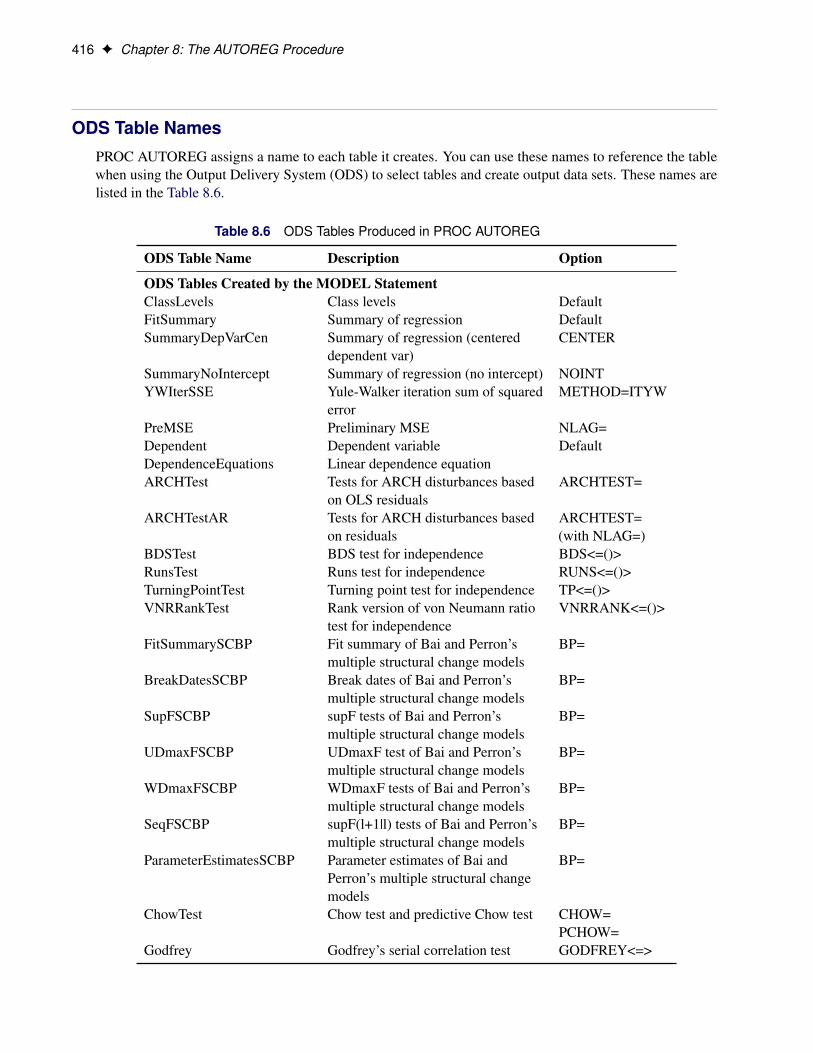
416 F Chapter 8: The AUTOREG Procedure
ODS Table NamesPROC AUTOREG assigns a name to each table it creates. You can use these names to reference the tablewhen using the Output Delivery System (ODS) to select tables and create output data sets. These names arelisted in the Table 8.6.
Table 8.6 ODS Tables Produced in PROC AUTOREG
ODS Table Name Description Option
ODS Tables Created by the MODEL StatementClassLevels Class levels DefaultFitSummary Summary of regression DefaultSummaryDepVarCen Summary of regression (centered
dependent var)CENTER
SummaryNoIntercept Summary of regression (no intercept) NOINTYWIterSSE Yule-Walker iteration sum of squared
errorMETHOD=ITYW
PreMSE Preliminary MSE NLAG=Dependent Dependent variable DefaultDependenceEquations Linear dependence equationARCHTest Tests for ARCH disturbances based
on OLS residualsARCHTEST=
ARCHTestAR Tests for ARCH disturbances basedon residuals
ARCHTEST=(with NLAG=)
BDSTest BDS test for independence BDS<=()>RunsTest Runs test for independence RUNS<=()>TurningPointTest Turning point test for independence TP<=()>VNRRankTest Rank version of von Neumann ratio
test for independenceVNRRANK<=()>
FitSummarySCBP Fit summary of Bai and Perron’smultiple structural change models
BP=
BreakDatesSCBP Break dates of Bai and Perron’smultiple structural change models
BP=
SupFSCBP supF tests of Bai and Perron’smultiple structural change models
BP=
UDmaxFSCBP UDmaxF test of Bai and Perron’smultiple structural change models
BP=
WDmaxFSCBP WDmaxF tests of Bai and Perron’smultiple structural change models
BP=
SeqFSCBP supF(l+1|l) tests of Bai and Perron’smultiple structural change models
BP=
ParameterEstimatesSCBP Parameter estimates of Bai andPerron’s multiple structural changemodels
BP=
ChowTest Chow test and predictive Chow test CHOW=PCHOW=
Godfrey Godfrey’s serial correlation test GODFREY<=>

ODS Table Names F 417
Table 8.6 continued
ODS Table Name Description Option
PhilPerron Phillips-Perron unit root test STATIONARITY=(PHILIPS<=()>)(no regressor)
PhilOul Phillips-Ouliaris cointegration test STATIONARITY=(PHILIPS<=()>)(has regressor)
ADF Augmented Dickey-Fuller unit roottest
STATIONARITY=(ADF<=()>) (noregressor)
EngleGranger Engle-Granger cointegration test STATIONARITY=(ADF<=()>) (hasregressor)
ERS ERS unit root test STATIONARITY=(ERS<=()>)
NgPerron Ng-Perron Unit root tests STATIONARITY=(NP=<()> )
KPSS Kwiatkowski, Phillips, Schmidt, andShin (KPSS) test or Shincointegration test
STATIONARITY=(KPSS<=()>)
ResetTest Ramsey’s RESET test RESETARParameterEstimates Estimates of autoregressive
parametersNLAG=
CorrGraph Estimates of autocorrelations NLAG=BackStep Backward elimination of
autoregressive termsBACKSTEP
ExpAutocorr Expected autocorrelations NLAG=IterHistory Iteration history ITPRINTParameterEstimates Parameter estimates DefaultParameterEstimatesGivenAR Parameter estimates assuming AR
parameters are givenNLAG=,METHOD= ULS |ML
PartialAutoCorr Partial autocorrelation PARTIALCovB Covariance of parameter estimates COVBCorrB Correlation of parameter estimates CORRBCholeskyFactor Cholesky root of gamma ALLCoefficients Coefficients for first NLAG
observationsCOEF
GammaInverse Gamma inverse GINVConvergenceStatus Convergence status table DefaultMiscStat Durbin t or Durbin h, Jarque-Bera
normality testLAGDEP=;NORMAL
DWTest Durbin-Watson statistics DW=

418 F Chapter 8: The AUTOREG Procedure
Table 8.6 continued
ODS Table Name Description Option
ODS Tables Created by the RESTRICT StatementRestrict Restriction table Default
ODS Tables Created by the TEST StatementFTest F test Default,
TYPE=ALLTestResults Wald, LM, LR tests TYPE=WALD |
LM (onlysupported withGARCH= option) |LR (onlysupported withGARCH= option)|ALL
ODS GraphicsStatistical procedures use ODS Graphics to create graphs as part of their output. ODS Graphics is describedin detail in Chapter 21, “Statistical Graphics Using ODS” (SAS/STAT User’s Guide).
Before you create graphs, ODS Graphics must be enabled (for example, with the ODS GRAPHICS ONstatement). For more information about enabling and disabling ODS Graphics, see the section “Enabling andDisabling ODS Graphics” in that chapter.
The overall appearance of graphs is controlled by ODS styles. Styles and other aspects of using ODSGraphics are discussed in the section “A Primer on ODS Statistical Graphics” in that chapter.
This section describes the use of ODS for creating graphics with the AUTOREG procedure.
To request these graphs, you must specify the ODS GRAPHICS statement. By default, only the residual,predicted versus actual, and autocorrelation of residuals plots are produced. If, in addition to the ODSGRAPHICS statement, you also specify the ALL option in either the PROC AUTOREG statement orMODEL statement, all plots are created. For HETERO, GARCH, and AR models studentized residuals arereplaced by standardized residuals. For the autoregressive models, the conditional variance of the residuals iscomputed as described in the section “Predicting Future Series Realizations” on page 410. For the GARCHand HETERO models, residuals are assumed to have ht conditional variance invoked by the HT= option ofthe OUTPUT statement. For all these cases, the Cook’s D plot is not produced.
ODS Graph Names
PROC AUTOREG assigns a name to each graph it creates using ODS. You can use these names to referencethe graphs when using ODS. The names are listed in Table 8.7.

Examples: AUTOREG Procedure F 419
Table 8.7 ODS Graphics Produced in PROC AUTOREG
ODS Table Name Description PLOTS= Option
DiagnosticsPanel All applicable plotsACFPlot Autocorrelation of residuals ACFAutoCorrPlot Estimates of autocorrelations AutoCorrPlotFitPlot Predicted versus actual plot FITPLOT, defaultCooksD Cook’s D plot COOKSD (no NLAG=)IACFPlot Inverse autocorrelation of residuals IACFQQPlot Q-Q plot of residuals QQPACFPlot Partial autocorrelation of residuals PACFResidualHistogram Histogram of the residuals RESIDUALHISTOGRAM
or RESIDHISTOGRAMResidualPlot Residual plot RESIDUAL or RES, defaultStudentResidualPlot Studentized residual plot STUDENTRESIDUAL (no
NLAG=, GARCH=, orHETERO)
StandardResidualPlot Standardized residual plot STANDARDRESIDUALWhiteNoiseLogProbPlot Tests for white noise residuals WHITENOISE
Examples: AUTOREG Procedure
Example 8.1: Analysis of Real Output SeriesIn this example, the annual real output series is analyzed over the period 1901 to 1983 (Balke and Gordon1986, pp. 581–583). With the following DATA step, the original data are transformed using the naturallogarithm, and the differenced series DY is created for further analysis. The log of real output is plotted inOutput 8.1.1.
title 'Analysis of Real GNP';data gnp;
date = intnx( 'year', '01jan1901'd, _n_-1 );format date year4.;input x @@;y = log(x);dy = dif(y);t = _n_;label y = 'Real GNP'
dy = 'First Difference of Y't = 'Time Trend';
datalines;137.87 139.13 146.10 144.21 155.04 172.97 175.61 161.22
... more lines ...

420 F Chapter 8: The AUTOREG Procedure
proc sgplot data=gnp noautolegend;scatter x=date y=y;xaxis grid values=('01jan1901'd '01jan1911'd '01jan1921'd '01jan1931'd
'01jan1941'd '01jan1951'd '01jan1961'd '01jan1971'd'01jan1981'd '01jan1991'd);
run;
Output 8.1.1 Real Output Series: 1901–1983
The (linear) trend-stationary process is estimated using the form
yt D ˇ0 C ˇ1t C �t
where
�t D �t � '1�t�1 � '2�t�2
�t�IN.0; ��/
The preceding trend-stationary model assumes that uncertainty over future horizons is bounded since theerror term, �t , has a finite variance. The maximum likelihood AR estimates from the statements that followare shown in Output 8.1.2:
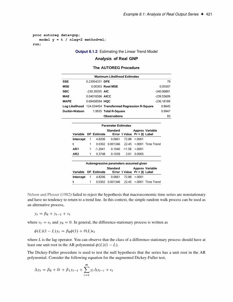
Example 8.1: Analysis of Real Output Series F 421
proc autoreg data=gnp;model y = t / nlag=2 method=ml;
run;
Output 8.1.2 Estimating the Linear Trend Model
Analysis of Real GNP
The AUTOREG Procedure
Maximum Likelihood Estimates
SSE 0.23954331 DFE 79
MSE 0.00303 Root MSE 0.05507
SBC -230.39355 AIC -240.06891
MAE 0.04016596 AICC -239.55609
MAPE 0.69458594 HQC -236.18189
Log Likelihood 124.034454 Transformed Regression R-Square 0.8645
Durbin-Watson 1.9935 Total R-Square 0.9947
Observations 83
Parameter Estimates
Variable DF EstimateStandard
Error t ValueApproxPr > |t|
VariableLabel
Intercept 1 4.8206 0.0661 72.88 <.0001
t 1 0.0302 0.001346 22.45 <.0001 Time Trend
AR1 1 -1.2041 0.1040 -11.58 <.0001
AR2 1 0.3748 0.1039 3.61 0.0005
Autoregressive parameters assumed given
Variable DF EstimateStandard
Error t ValueApproxPr > |t|
VariableLabel
Intercept 1 4.8206 0.0661 72.88 <.0001
t 1 0.0302 0.001346 22.45 <.0001 Time Trend
Nelson and Plosser (1982) failed to reject the hypothesis that macroeconomic time series are nonstationaryand have no tendency to return to a trend line. In this context, the simple random walk process can be used asan alternative process,
yt D ˇ0 C yt�1 C �t
where �t D �t and y0 D 0. In general, the difference-stationary process is written as
�.L/.1 � L/yt D ˇ0�.1/C �.L/�t
where L is the lag operator. You can observe that the class of a difference-stationary process should have atleast one unit root in the AR polynomial �.L/.1 � L/.
The Dickey-Fuller procedure is used to test the null hypothesis that the series has a unit root in the ARpolynomial. Consider the following equation for the augmented Dickey-Fuller test,
�yt D ˇ0 C ıt C ˇ1yt�1 C
mXiD1
i�yt�i C �t

422 F Chapter 8: The AUTOREG Procedure
where � D 1 � L. The test statistic �� is the usual t ratio for the parameter estimate O1, but the �� does notfollow a t distribution.
The following code performs the augmented Dickey-Fuller test with m D 3 and we are interesting in the testresults in the linear time trend case since the previous plot reveals there is a linear trend.
proc autoreg data = gnp;model y = / stationarity =(adf =3);
run;
The augmented Dickey-Fuller test indicates that the output series may have a difference-stationary process.The statistic Tau with linear time trend has a value of -2.6190 and its p-value is 0.2732. The statistic Rho hasa p-value of 0.0817, which also indicates the null of unit root is accepted at the 5% level. (See Output 8.1.3.)
Output 8.1.3 Augmented Dickey-Fuller Test Results
Analysis of Real GNP
The AUTOREG Procedure
Augmented Dickey-Fuller Unit Root Tests
Type Lags Rho Pr < Rho Tau Pr < Tau F Pr > F
Zero Mean 3 0.3827 0.7732 3.3342 0.9997
Single Mean 3 -0.1674 0.9465 -0.2046 0.9326 5.7521 0.0211
Trend 3 -18.0246 0.0817 -2.6190 0.2732 3.4472 0.4957
The AR(1) model for the differenced series DY is estimated using the maximum likelihood method for theperiod 1902 to 1983. The difference-stationary process is written
�yt D ˇ0 C �t
�t D �t � '1�t�1
The estimated value of '1 is �0:297 and that of ˇ0 is 0.0293. All estimated values are statistically significant.The PROC step follows:
proc autoreg data=gnp;model dy = / nlag=1 method=ml;
run;
The printed output produced by the PROC step is shown in Output 8.1.4.

Example 8.2: Comparing Estimates and Models F 423
Output 8.1.4 Estimating the Differenced Series with AR(1) Error
Analysis of Real GNP
The AUTOREG Procedure
Maximum Likelihood Estimates
SSE 0.27107673 DFE 80
MSE 0.00339 Root MSE 0.05821
SBC -226.77848 AIC -231.59192
MAE 0.04333026 AICC -231.44002
MAPE 153.637587 HQC -229.65939
Log Likelihood 117.795958 Transformed Regression R-Square 0.0000
Durbin-Watson 1.9268 Total R-Square 0.0900
Observations 82
Parameter Estimates
Variable DF EstimateStandard
Error t ValueApproxPr > |t|
Intercept 1 0.0293 0.009093 3.22 0.0018
AR1 1 -0.2967 0.1067 -2.78 0.0067
Autoregressive parameters assumed given
Variable DF EstimateStandard
Error t ValueApproxPr > |t|
Intercept 1 0.0293 0.009093 3.22 0.0018
Example 8.2: Comparing Estimates and ModelsIn this example, the Grunfeld series are estimated using different estimation methods. For information aboutthe Grunfeld investment data set, see Maddala (1977). For comparison, the Yule-Walker method, ULSmethod, and maximum likelihood method estimates are shown. With the DWPROB option, the p-value ofthe Durbin-Watson statistic is printed. The Durbin-Watson test indicates the positive autocorrelation of theregression residuals. The DATA and PROC steps follow:
title 'Grunfeld''s Investment Models Fit with Autoregressive Errors';data grunfeld;
input year gei gef gec;label gei = 'Gross investment GE'
gec = 'Lagged Capital Stock GE'gef = 'Lagged Value of GE shares';
datalines;1935 33.1 1170.6 97.8
... more lines ...
proc autoreg data=grunfeld;model gei = gef gec / nlag=1 dwprob;model gei = gef gec / nlag=1 method=uls;model gei = gef gec / nlag=1 method=ml;
run;
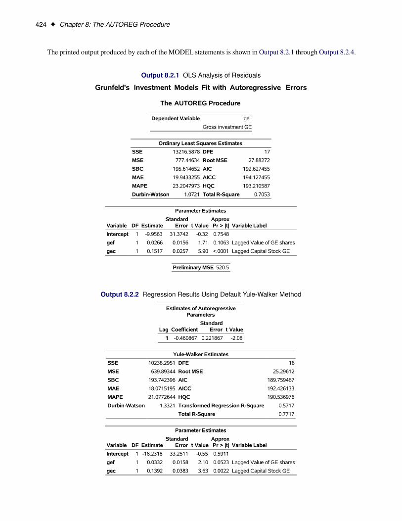
424 F Chapter 8: The AUTOREG Procedure
The printed output produced by each of the MODEL statements is shown in Output 8.2.1 through Output 8.2.4.
Output 8.2.1 OLS Analysis of Residuals
Grunfeld's Investment Models Fit with Autoregressive Errors
The AUTOREG Procedure
Dependent Variable gei
Gross investment GE
Ordinary Least Squares Estimates
SSE 13216.5878 DFE 17
MSE 777.44634 Root MSE 27.88272
SBC 195.614652 AIC 192.627455
MAE 19.9433255 AICC 194.127455
MAPE 23.2047973 HQC 193.210587
Durbin-Watson 1.0721 Total R-Square 0.7053
Parameter Estimates
Variable DF EstimateStandard
Error t ValueApproxPr > |t| Variable Label
Intercept 1 -9.9563 31.3742 -0.32 0.7548
gef 1 0.0266 0.0156 1.71 0.1063 Lagged Value of GE shares
gec 1 0.1517 0.0257 5.90 <.0001 Lagged Capital Stock GE
Preliminary MSE 520.5
Output 8.2.2 Regression Results Using Default Yule-Walker Method
Estimates of AutoregressiveParameters
Lag CoefficientStandard
Error t Value
1 -0.460867 0.221867 -2.08
Yule-Walker Estimates
SSE 10238.2951 DFE 16
MSE 639.89344 Root MSE 25.29612
SBC 193.742396 AIC 189.759467
MAE 18.0715195 AICC 192.426133
MAPE 21.0772644 HQC 190.536976
Durbin-Watson 1.3321 Transformed Regression R-Square 0.5717
Total R-Square 0.7717
Parameter Estimates
Variable DF EstimateStandard
Error t ValueApproxPr > |t| Variable Label
Intercept 1 -18.2318 33.2511 -0.55 0.5911
gef 1 0.0332 0.0158 2.10 0.0523 Lagged Value of GE shares
gec 1 0.1392 0.0383 3.63 0.0022 Lagged Capital Stock GE
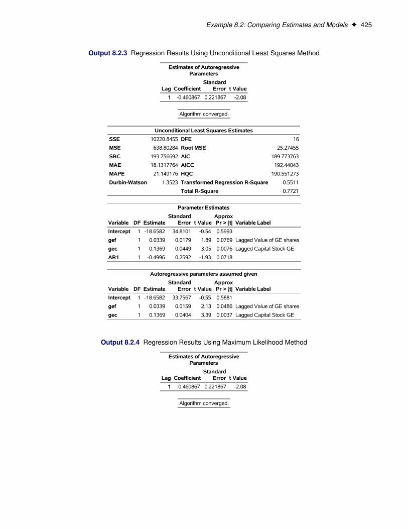
Example 8.2: Comparing Estimates and Models F 425
Output 8.2.3 Regression Results Using Unconditional Least Squares Method
Estimates of AutoregressiveParameters
Lag CoefficientStandard
Error t Value
1 -0.460867 0.221867 -2.08
Algorithm converged.
Unconditional Least Squares Estimates
SSE 10220.8455 DFE 16
MSE 638.80284 Root MSE 25.27455
SBC 193.756692 AIC 189.773763
MAE 18.1317764 AICC 192.44043
MAPE 21.149176 HQC 190.551273
Durbin-Watson 1.3523 Transformed Regression R-Square 0.5511
Total R-Square 0.7721
Parameter Estimates
Variable DF EstimateStandard
Error t ValueApproxPr > |t| Variable Label
Intercept 1 -18.6582 34.8101 -0.54 0.5993
gef 1 0.0339 0.0179 1.89 0.0769 Lagged Value of GE shares
gec 1 0.1369 0.0449 3.05 0.0076 Lagged Capital Stock GE
AR1 1 -0.4996 0.2592 -1.93 0.0718
Autoregressive parameters assumed given
Variable DF EstimateStandard
Error t ValueApproxPr > |t| Variable Label
Intercept 1 -18.6582 33.7567 -0.55 0.5881
gef 1 0.0339 0.0159 2.13 0.0486 Lagged Value of GE shares
gec 1 0.1369 0.0404 3.39 0.0037 Lagged Capital Stock GE
Output 8.2.4 Regression Results Using Maximum Likelihood Method
Estimates of AutoregressiveParameters
Lag CoefficientStandard
Error t Value
1 -0.460867 0.221867 -2.08
Algorithm converged.

426 F Chapter 8: The AUTOREG Procedure
Output 8.2.4 continued
Maximum Likelihood Estimates
SSE 10229.2303 DFE 16
MSE 639.32689 Root MSE 25.28491
SBC 193.738877 AIC 189.755947
MAE 18.0892426 AICC 192.422614
MAPE 21.0978407 HQC 190.533457
Log Likelihood -90.877974 Transformed Regression R-Square 0.5656
Durbin-Watson 1.3385 Total R-Square 0.7719
Observations 20
Parameter Estimates
Variable DF EstimateStandard
Error t ValueApproxPr > |t| Variable Label
Intercept 1 -18.3751 34.5941 -0.53 0.6026
gef 1 0.0334 0.0179 1.87 0.0799 Lagged Value of GE shares
gec 1 0.1385 0.0428 3.23 0.0052 Lagged Capital Stock GE
AR1 1 -0.4728 0.2582 -1.83 0.0858
Autoregressive parameters assumed given
Variable DF EstimateStandard
Error t ValueApproxPr > |t| Variable Label
Intercept 1 -18.3751 33.3931 -0.55 0.5897
gef 1 0.0334 0.0158 2.11 0.0512 Lagged Value of GE shares
gec 1 0.1385 0.0389 3.56 0.0026 Lagged Capital Stock GE
Output 8.2.5 Estimates of Autocorrelations

Example 8.3: Lack-of-Fit Study F 427
Example 8.3: Lack-of-Fit StudyMany time series exhibit high positive autocorrelation, having the smooth appearance of a random walk. Thisbehavior can be explained by the partial adjustment and adaptive expectation hypotheses.
Short-term forecasting applications often use autoregressive models because these models absorb the behaviorof this kind of data. In the case of a first-order AR process where the autoregressive parameter is exactly 1 (arandom walk ), the best prediction of the future is the immediate past.
PROC AUTOREG can often greatly improve the fit of models, not only by adding additional parameters butalso by capturing the random walk tendencies. Thus, PROC AUTOREG can be expected to provide goodshort-term forecast predictions.
However, good forecasts do not necessarily mean that your structural model contributes anything worthwhileto the fit. In the following example, random noise is fit to part of a sine wave. Notice that the structural modeldoes not fit at all, but the autoregressive process does quite well and is very nearly a first difference (AR(1) =�:976). The DATA step, PROC AUTOREG step, and PROC SGPLOT step follow:
title1 'Lack of Fit Study';title2 'Fitting White Noise Plus Autoregressive Errors to a Sine Wave';
data a;pi=3.14159;do time = 1 to 75;
if time > 75 then y = .;else y = sin( pi * ( time / 50 ) );x = ranuni( 1234567 );output;
end;run;
proc autoreg data=a plots;model y = x / nlag=1;output out=b p=pred pm=xbeta;
run;
proc sgplot data=b;scatter y=y x=time / markerattrs=(color=black);series y=pred x=time / lineattrs=(color=blue);series y=xbeta x=time / lineattrs=(color=red);
run;
The printed output produced by PROC AUTOREG is shown in Output 8.3.1 and Output 8.3.2. Plots ofobserved and predicted values are shown in Output 8.3.3 and Output 8.3.4. Note: the plot Output 8.3.3 canbe viewed in the Autoreg.Model.FitDiagnosticPlots category by selecting ViewIResults.
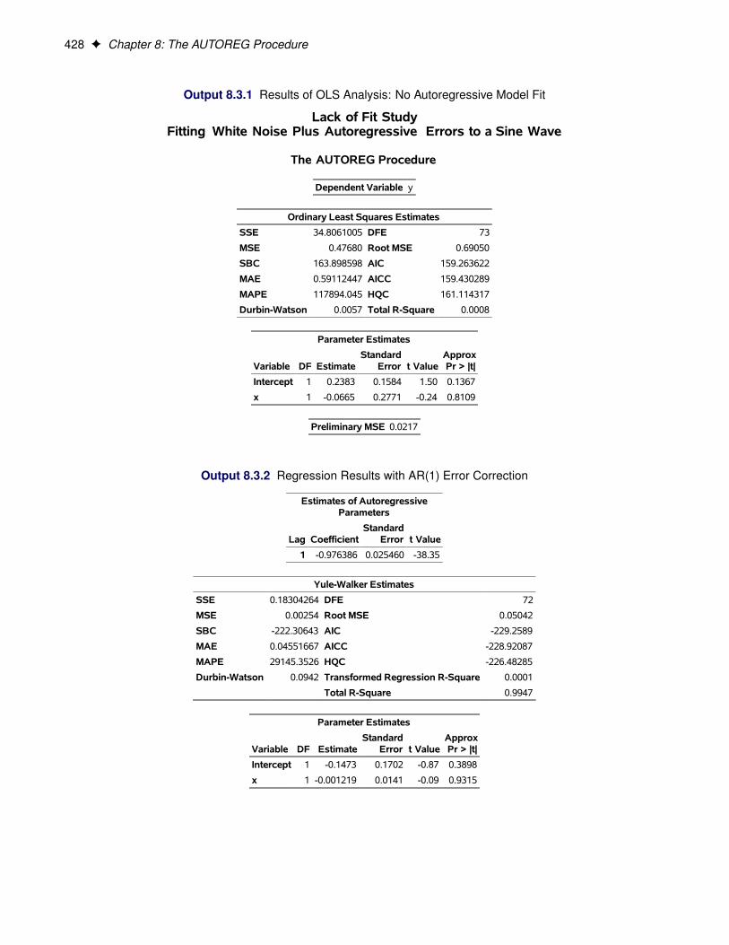
428 F Chapter 8: The AUTOREG Procedure
Output 8.3.1 Results of OLS Analysis: No Autoregressive Model Fit
Lack of Fit StudyFitting White Noise Plus Autoregressive Errors to a Sine Wave
The AUTOREG Procedure
Dependent Variable y
Ordinary Least Squares Estimates
SSE 34.8061005 DFE 73
MSE 0.47680 Root MSE 0.69050
SBC 163.898598 AIC 159.263622
MAE 0.59112447 AICC 159.430289
MAPE 117894.045 HQC 161.114317
Durbin-Watson 0.0057 Total R-Square 0.0008
Parameter Estimates
Variable DF EstimateStandard
Error t ValueApproxPr > |t|
Intercept 1 0.2383 0.1584 1.50 0.1367
x 1 -0.0665 0.2771 -0.24 0.8109
Preliminary MSE 0.0217
Output 8.3.2 Regression Results with AR(1) Error Correction
Estimates of AutoregressiveParameters
Lag CoefficientStandard
Error t Value
1 -0.976386 0.025460 -38.35
Yule-Walker Estimates
SSE 0.18304264 DFE 72
MSE 0.00254 Root MSE 0.05042
SBC -222.30643 AIC -229.2589
MAE 0.04551667 AICC -228.92087
MAPE 29145.3526 HQC -226.48285
Durbin-Watson 0.0942 Transformed Regression R-Square 0.0001
Total R-Square 0.9947
Parameter Estimates
Variable DF EstimateStandard
Error t ValueApproxPr > |t|
Intercept 1 -0.1473 0.1702 -0.87 0.3898
x 1 -0.001219 0.0141 -0.09 0.9315
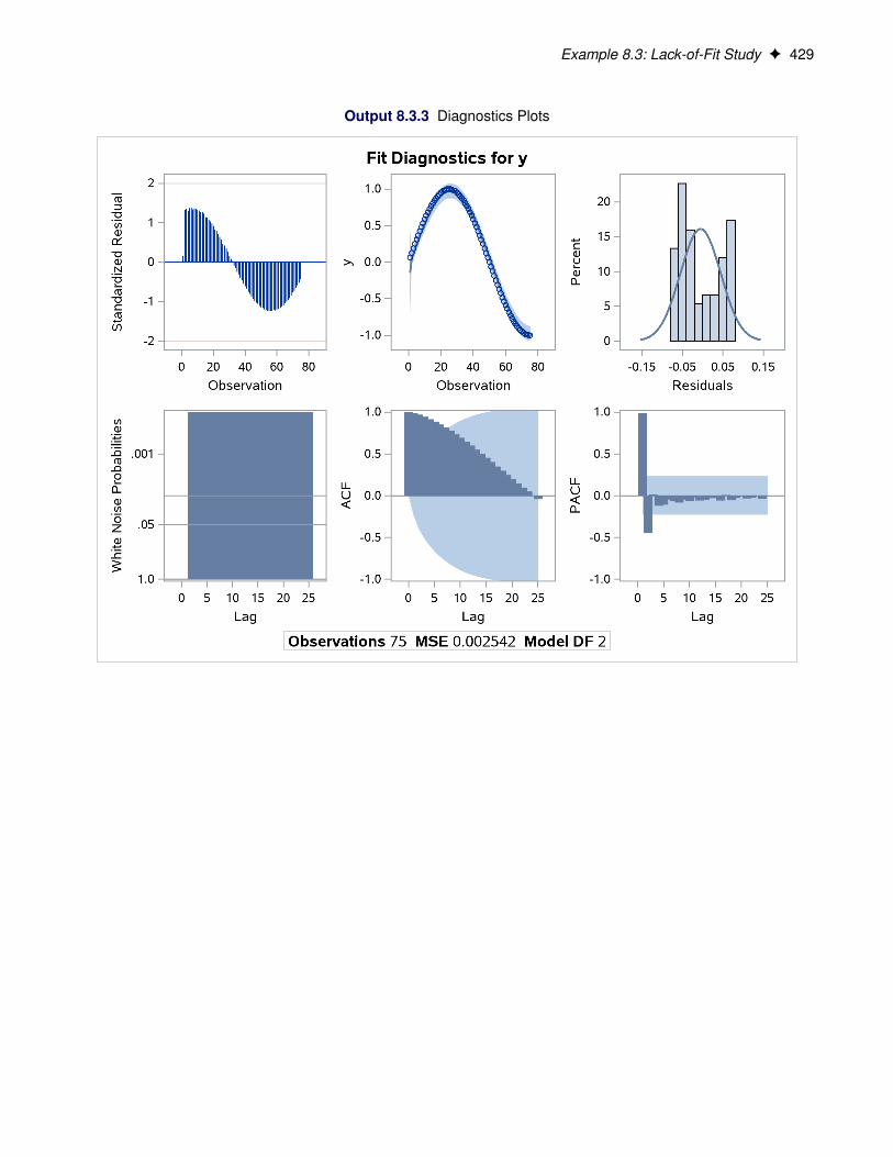
Example 8.3: Lack-of-Fit Study F 429
Output 8.3.3 Diagnostics Plots

430 F Chapter 8: The AUTOREG Procedure
Output 8.3.4 Plot of Autoregressive Prediction
Output 8.3.5 Estimates of Autocorrelations
Example 8.4: Missing ValuesIn this example, a pure autoregressive error model with no regressors is used to generate 50 values of a timeseries. Approximately 15% of the values are randomly chosen and set to missing. The following statementsgenerate the data:

Example 8.4: Missing Values F 431
title 'Simulated Time Series with Roots:';title2 ' (X-1.25)(X**4-1.25)';title3 'With 15% Missing Values';data ar;
do i=1 to 550;e = rannor(12345);n = sum( e, .8*n1, .8*n4, -.64*n5 ); /* ar process */y = n;if ranuni(12345) > .85 then y = .; /* 15% missing */n5=n4; n4=n3; n3=n2; n2=n1; n1=n; /* set lags */if i>500 then output;
end;run;
The model is estimated using maximum likelihood, and the residuals are plotted with 99% confidence limits.The PARTIAL option prints the partial autocorrelations. The following statements fit the model:
proc autoreg data=ar partial;model y = / nlag=(1 4 5) method=ml;output out=a predicted=p residual=r ucl=u lcl=l alphacli=.01;
run;
The printed output produced by the AUTOREG procedure is shown in Output 8.4.1 and Output 8.4.2.Note: the plot Output 8.4.2 can be viewed in the Autoreg.Model.FitDiagnosticPlots category by selectingViewIResults.
Output 8.4.1 Autocorrelation-Corrected Regression Results
Simulated Time Series with Roots:(X-1.25)(X**4-1.25)
With 15% Missing Values
The AUTOREG Procedure
Dependent Variable y
Ordinary Least Squares Estimates
SSE 182.972379 DFE 40
MSE 4.57431 Root MSE 2.13876
SBC 181.39282 AIC 179.679248
MAE 1.80469152 AICC 179.781813
MAPE 270.104379 HQC 180.303237
Durbin-Watson 1.3962 Total R-Square 0.0000
Parameter Estimates
Variable DF EstimateStandard
Error t ValueApproxPr > |t|
Intercept 1 -2.2387 0.3340 -6.70 <.0001
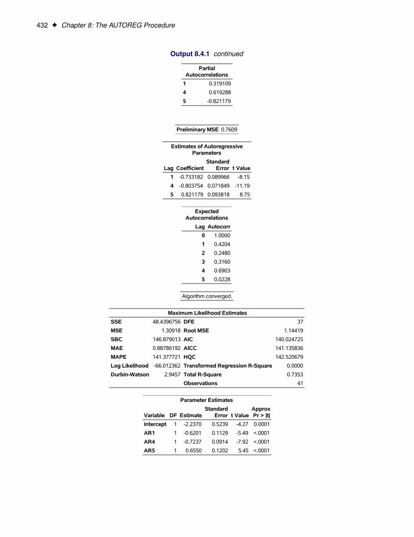
432 F Chapter 8: The AUTOREG Procedure
Output 8.4.1 continued
PartialAutocorrelations
1 0.319109
4 0.619288
5 -0.821179
Preliminary MSE 0.7609
Estimates of AutoregressiveParameters
Lag CoefficientStandard
Error t Value
1 -0.733182 0.089966 -8.15
4 -0.803754 0.071849 -11.19
5 0.821179 0.093818 8.75
ExpectedAutocorrelations
Lag Autocorr
0 1.0000
1 0.4204
2 0.2480
3 0.3160
4 0.6903
5 0.0228
Algorithm converged.
Maximum Likelihood Estimates
SSE 48.4396756 DFE 37
MSE 1.30918 Root MSE 1.14419
SBC 146.879013 AIC 140.024725
MAE 0.88786192 AICC 141.135836
MAPE 141.377721 HQC 142.520679
Log Likelihood -66.012362 Transformed Regression R-Square 0.0000
Durbin-Watson 2.9457 Total R-Square 0.7353
Observations 41
Parameter Estimates
Variable DF EstimateStandard
Error t ValueApproxPr > |t|
Intercept 1 -2.2370 0.5239 -4.27 0.0001
AR1 1 -0.6201 0.1129 -5.49 <.0001
AR4 1 -0.7237 0.0914 -7.92 <.0001
AR5 1 0.6550 0.1202 5.45 <.0001
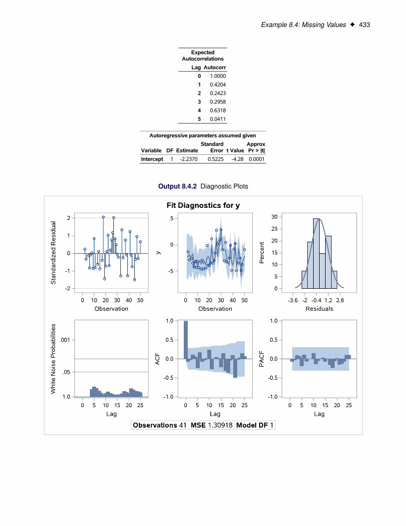
Example 8.4: Missing Values F 433
ExpectedAutocorrelations
Lag Autocorr
0 1.0000
1 0.4204
2 0.2423
3 0.2958
4 0.6318
5 0.0411
Autoregressive parameters assumed given
Variable DF EstimateStandard
Error t ValueApproxPr > |t|
Intercept 1 -2.2370 0.5225 -4.28 0.0001
Output 8.4.2 Diagnostic Plots

434 F Chapter 8: The AUTOREG Procedure
Output 8.4.3 Estimates of Autocorrelations
The following statements plot the residuals and confidence limits:
data reshape1;set a;miss = .;if r=. then do;
miss = p;p = .;
end;run;
title 'Predicted Values and Confidence Limits';
proc sgplot data=reshape1 NOAUTOLEGEND;band x=i upper=u lower=l;scatter y=miss x=i/ MARKERATTRS =(symbol=x color=red);series y=p x=i/markers MARKERATTRS =(color=blue) lineattrs=(color=blue);
run;
The plot of the predicted values and the upper and lower confidence limits is shown in Output 8.4.4. Notethat the confidence interval is wider at the beginning of the series (when there are no past noise values to usein the forecast equation) and after missing values where, again, there is an incomplete set of past residuals.
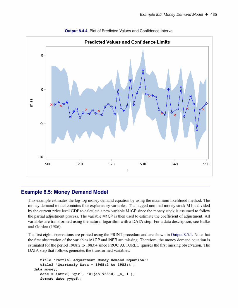
Example 8.5: Money Demand Model F 435
Output 8.4.4 Plot of Predicted Values and Confidence Interval
Example 8.5: Money Demand ModelThis example estimates the log-log money demand equation by using the maximum likelihood method. Themoney demand model contains four explanatory variables. The lagged nominal money stock M1 is dividedby the current price level GDF to calculate a new variable M1CP since the money stock is assumed to followthe partial adjustment process. The variable M1CP is then used to estimate the coefficient of adjustment. Allvariables are transformed using the natural logarithm with a DATA step. For a data description, see Balkeand Gordon (1986).
The first eight observations are printed using the PRINT procedure and are shown in Output 8.5.1. Note thatthe first observation of the variables M1CP and INFR are missing. Therefore, the money demand equation isestimated for the period 1968:2 to 1983:4 since PROC AUTOREG ignores the first missing observation. TheDATA step that follows generates the transformed variables:
title 'Partial Adjustment Money Demand Equation';title2 'Quarterly Data - 1968:2 to 1983:4';
data money;date = intnx( 'qtr', '01jan1968'd, _n_-1 );format date yyqc6.;
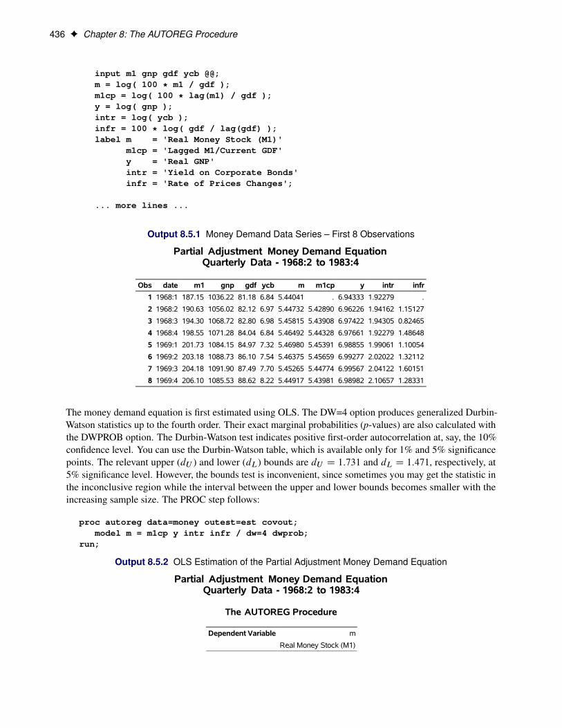
436 F Chapter 8: The AUTOREG Procedure
input m1 gnp gdf ycb @@;m = log( 100 * m1 / gdf );m1cp = log( 100 * lag(m1) / gdf );y = log( gnp );intr = log( ycb );infr = 100 * log( gdf / lag(gdf) );label m = 'Real Money Stock (M1)'
m1cp = 'Lagged M1/Current GDF'y = 'Real GNP'intr = 'Yield on Corporate Bonds'infr = 'Rate of Prices Changes';
... more lines ...
Output 8.5.1 Money Demand Data Series – First 8 Observations
Partial Adjustment Money Demand EquationQuarterly Data - 1968:2 to 1983:4
Obs date m1 gnp gdf ycb m m1cp y intr infr
1 1968:1 187.15 1036.22 81.18 6.84 5.44041 . 6.94333 1.92279 .
2 1968:2 190.63 1056.02 82.12 6.97 5.44732 5.42890 6.96226 1.94162 1.15127
3 1968:3 194.30 1068.72 82.80 6.98 5.45815 5.43908 6.97422 1.94305 0.82465
4 1968:4 198.55 1071.28 84.04 6.84 5.46492 5.44328 6.97661 1.92279 1.48648
5 1969:1 201.73 1084.15 84.97 7.32 5.46980 5.45391 6.98855 1.99061 1.10054
6 1969:2 203.18 1088.73 86.10 7.54 5.46375 5.45659 6.99277 2.02022 1.32112
7 1969:3 204.18 1091.90 87.49 7.70 5.45265 5.44774 6.99567 2.04122 1.60151
8 1969:4 206.10 1085.53 88.62 8.22 5.44917 5.43981 6.98982 2.10657 1.28331
The money demand equation is first estimated using OLS. The DW=4 option produces generalized Durbin-Watson statistics up to the fourth order. Their exact marginal probabilities (p-values) are also calculated withthe DWPROB option. The Durbin-Watson test indicates positive first-order autocorrelation at, say, the 10%confidence level. You can use the Durbin-Watson table, which is available only for 1% and 5% significancepoints. The relevant upper (dU ) and lower (dL) bounds are dU D 1:731 and dL D 1:471, respectively, at5% significance level. However, the bounds test is inconvenient, since sometimes you may get the statistic inthe inconclusive region while the interval between the upper and lower bounds becomes smaller with theincreasing sample size. The PROC step follows:
proc autoreg data=money outest=est covout;model m = m1cp y intr infr / dw=4 dwprob;
run;
Output 8.5.2 OLS Estimation of the Partial Adjustment Money Demand Equation
Partial Adjustment Money Demand EquationQuarterly Data - 1968:2 to 1983:4
The AUTOREG Procedure
Dependent Variable m
Real Money Stock (M1)

Example 8.5: Money Demand Model F 437
Output 8.5.2 continued
Ordinary Least Squares Estimates
SSE 0.00271902 DFE 58
MSE 0.0000469 Root MSE 0.00685
SBC -433.68709 AIC -444.40276
MAE 0.00483389 AICC -443.35013
MAPE 0.08888324 HQC -440.18824
Total R-Square 0.9546
Durbin-Watson Statistics
Order DW Pr < DW Pr > DW
1 1.7355 0.0607 0.9393
2 2.1058 0.5519 0.4481
3 2.0286 0.5002 0.4998
4 2.2835 0.8880 0.1120
NOTE: Pr<DW is the p-value for testing positive autocorrelation, and Pr>DW is the p-value fortesting negative autocorrelation.
Parameter Estimates
Variable DF EstimateStandard
Error t ValueApproxPr > |t| Variable Label
Intercept 1 0.3084 0.2359 1.31 0.1963
m1cp 1 0.8952 0.0439 20.38 <.0001 Lagged M1/Current GDF
y 1 0.0476 0.0122 3.89 0.0003 Real GNP
intr 1 -0.0238 0.007933 -3.00 0.0040 Yield on Corporate Bonds
infr 1 -0.005646 0.001584 -3.56 0.0007 Rate of Prices Changes
The autoregressive model is estimated using the maximum likelihood method. Though the Durbin-Watsontest statistic is calculated after correcting the autocorrelation, it should be used with care since the test basedon this statistic is not justified theoretically. The PROC step follows:
proc autoreg data=money;model m = m1cp y intr infr / nlag=1 method=ml maxit=50;output out=a p=p pm=pm r=r rm=rm ucl=ucl lcl=lcl
uclm=uclm lclm=lclm;run;
proc print data=a(obs=8);var p pm r rm ucl lcl uclm lclm;
run;
A difference is shown between the OLS estimates in Output 8.5.2 and the AR(1)-ML estimates in Output 8.5.3.The estimated autocorrelation coefficient is significantly negative .�0:88345/. Note that the negativecoefficient of AR(1) should be interpreted as a positive autocorrelation.
Two predicted values are produced: predicted values computed for the structural model and predicted valuescomputed for the full model. The full model includes both the structural and error-process parts. Thepredicted values and residuals are stored in the output data set A, as are the upper and lower 95% confidencelimits for the predicted values. Part of the data set A is shown in Output 8.5.4. The first observation is missingsince the explanatory variables, M1CP and INFR, are missing for the corresponding observation.

438 F Chapter 8: The AUTOREG Procedure
Output 8.5.3 Estimated Partial Adjustment Money Demand Equation
Partial Adjustment Money Demand EquationQuarterly Data - 1968:2 to 1983:4
The AUTOREG Procedure
Estimates of AutoregressiveParameters
Lag CoefficientStandard
Error t Value
1 -0.126273 0.131393 -0.96
Algorithm converged.
Maximum Likelihood Estimates
SSE 0.00226719 DFE 57
MSE 0.0000398 Root MSE 0.00631
SBC -439.47665 AIC -452.33545
MAE 0.00506044 AICC -450.83545
MAPE 0.09302277 HQC -447.27802
Log Likelihood 232.167727 Transformed Regression R-Square 0.6954
Durbin-Watson 2.1778 Total R-Square 0.9621
Observations 63
Parameter Estimates
Variable DF EstimateStandard
Error t ValueApproxPr > |t| Variable Label
Intercept 1 2.4121 0.4880 4.94 <.0001
m1cp 1 0.4086 0.0908 4.50 <.0001 Lagged M1/Current GDF
y 1 0.1509 0.0411 3.67 0.0005 Real GNP
intr 1 -0.1101 0.0159 -6.92 <.0001 Yield on Corporate Bonds
infr 1 -0.006348 0.001834 -3.46 0.0010 Rate of Prices Changes
AR1 1 -0.8835 0.0686 -12.89 <.0001
Autoregressive parameters assumed given
Variable DF EstimateStandard
Error t ValueApproxPr > |t| Variable Label
Intercept 1 2.4121 0.4685 5.15 <.0001
m1cp 1 0.4086 0.0840 4.87 <.0001 Lagged M1/Current GDF
y 1 0.1509 0.0402 3.75 0.0004 Real GNP
intr 1 -0.1101 0.0155 -7.08 <.0001 Yield on Corporate Bonds
infr 1 -0.006348 0.001828 -3.47 0.0010 Rate of Prices Changes
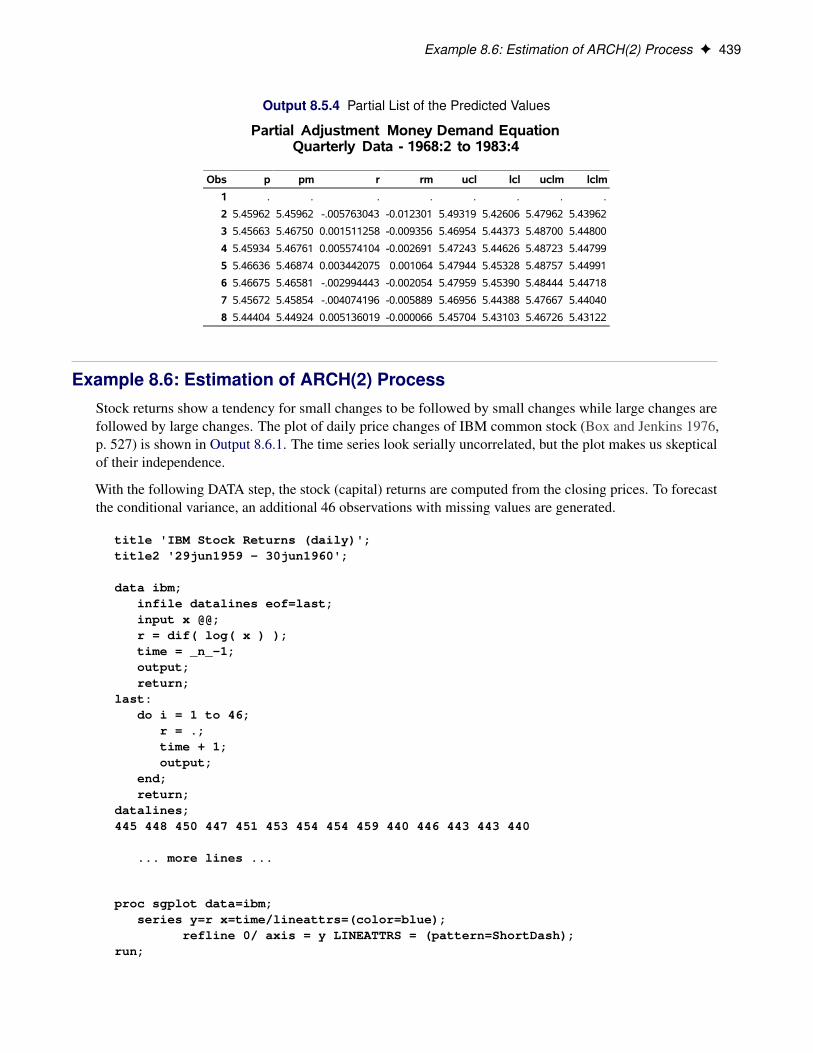
Example 8.6: Estimation of ARCH(2) Process F 439
Output 8.5.4 Partial List of the Predicted Values
Partial Adjustment Money Demand EquationQuarterly Data - 1968:2 to 1983:4
Obs p pm r rm ucl lcl uclm lclm
1 . . . . . . . .
2 5.45962 5.45962 -.005763043 -0.012301 5.49319 5.42606 5.47962 5.43962
3 5.45663 5.46750 0.001511258 -0.009356 5.46954 5.44373 5.48700 5.44800
4 5.45934 5.46761 0.005574104 -0.002691 5.47243 5.44626 5.48723 5.44799
5 5.46636 5.46874 0.003442075 0.001064 5.47944 5.45328 5.48757 5.44991
6 5.46675 5.46581 -.002994443 -0.002054 5.47959 5.45390 5.48444 5.44718
7 5.45672 5.45854 -.004074196 -0.005889 5.46956 5.44388 5.47667 5.44040
8 5.44404 5.44924 0.005136019 -0.000066 5.45704 5.43103 5.46726 5.43122
Example 8.6: Estimation of ARCH(2) ProcessStock returns show a tendency for small changes to be followed by small changes while large changes arefollowed by large changes. The plot of daily price changes of IBM common stock (Box and Jenkins 1976,p. 527) is shown in Output 8.6.1. The time series look serially uncorrelated, but the plot makes us skepticalof their independence.
With the following DATA step, the stock (capital) returns are computed from the closing prices. To forecastthe conditional variance, an additional 46 observations with missing values are generated.
title 'IBM Stock Returns (daily)';title2 '29jun1959 - 30jun1960';
data ibm;infile datalines eof=last;input x @@;r = dif( log( x ) );time = _n_-1;output;return;
last:do i = 1 to 46;
r = .;time + 1;output;
end;return;
datalines;445 448 450 447 451 453 454 454 459 440 446 443 443 440
... more lines ...
proc sgplot data=ibm;series y=r x=time/lineattrs=(color=blue);
refline 0/ axis = y LINEATTRS = (pattern=ShortDash);run;
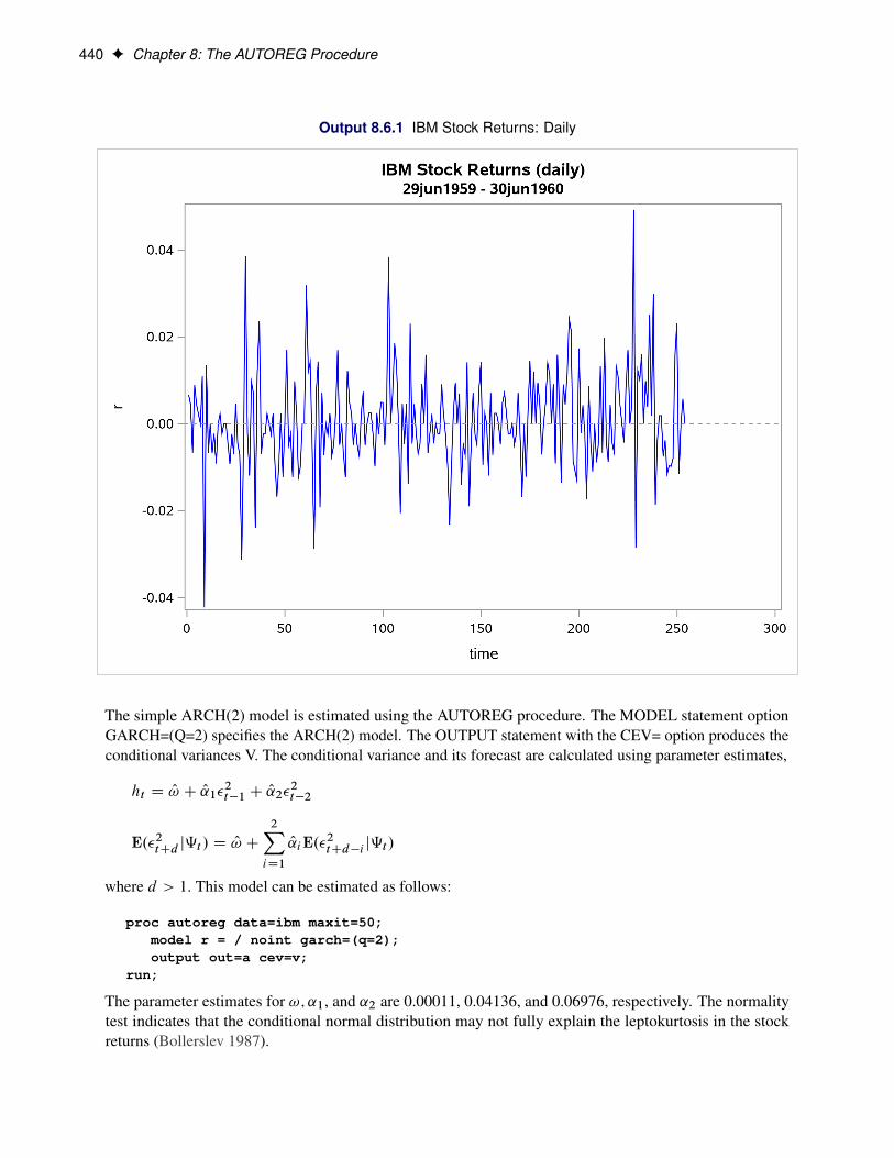
440 F Chapter 8: The AUTOREG Procedure
Output 8.6.1 IBM Stock Returns: Daily
The simple ARCH(2) model is estimated using the AUTOREG procedure. The MODEL statement optionGARCH=(Q=2) specifies the ARCH(2) model. The OUTPUT statement with the CEV= option produces theconditional variances V. The conditional variance and its forecast are calculated using parameter estimates,
ht D O! C O1�2t�1 C O2�
2t�2
E.�2tCd j‰t / D O! C2XiD1
O iE.�2tCd�i j‰t /
where d > 1: This model can be estimated as follows:
proc autoreg data=ibm maxit=50;model r = / noint garch=(q=2);output out=a cev=v;
run;
The parameter estimates for !; ˛1, and ˛2 are 0.00011, 0.04136, and 0.06976, respectively. The normalitytest indicates that the conditional normal distribution may not fully explain the leptokurtosis in the stockreturns (Bollerslev 1987).

Example 8.6: Estimation of ARCH(2) Process F 441
The ARCH model estimates are shown in Output 8.6.2, and conditional variances are also shown in Out-put 8.6.3. The following code generates Output 8.6.3:
data b; set a;length type $ 8.;if r ^= . then do;
type = 'ESTIMATE'; output; end;else do;
type = 'FORECAST'; output; end;run;proc sgplot data=b;
series x=time y=v/group=type;refline 254/ axis = x LINEATTRS = (pattern=ShortDash);
run;
Output 8.6.2 ARCH(2) Estimation Results
IBM Stock Returns (daily)29jun1959 - 30jun1960
The AUTOREG Procedure
Dependent Variable r
Ordinary Least Squares Estimates
SSE 0.03214307 DFE 254
MSE 0.0001265 Root MSE 0.01125
SBC -1558.802 AIC -1558.802
MAE 0.00814086 AICC -1558.802
MAPE 100.378566 HQC -1558.802
Durbin-Watson 2.1377 Total R-Square 0.0000
NOTE: No intercept term is used.R-squares are redefined.
Algorithm converged.
GARCH Estimates
SSE 0.03214307 Observations 254
MSE 0.0001265 Uncond Var 0.00012632
Log Likelihood 781.017441 Total R-Square 0.0000
SBC -1545.4229 AIC -1556.0349
MAE 0.00805675 AICC -1555.9389
MAPE 100 HQC -1551.7658
Normality Test 105.8587
Pr > ChiSq <.0001
NOTE: No intercept term is used.R-squares are redefined.

442 F Chapter 8: The AUTOREG Procedure
Output 8.6.2 continued
Parameter Estimates
Variable DF EstimateStandard
Error t ValueApproxPr > |t|
ARCH0 1 0.000112 7.6059E-6 14.76 <.0001
ARCH1 1 0.0414 0.0514 0.81 0.4208
ARCH2 1 0.0698 0.0434 1.61 0.1082
Output 8.6.3 Conditional Variance for IBM Stock Prices
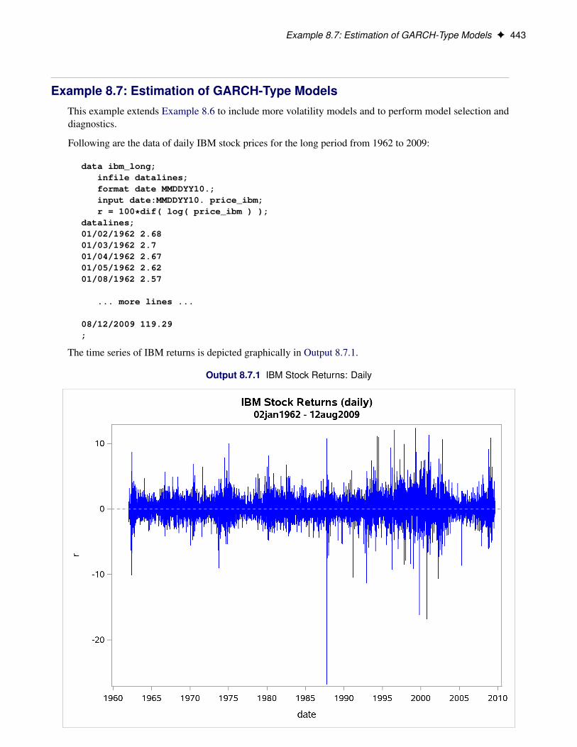
Example 8.7: Estimation of GARCH-Type Models F 443
Example 8.7: Estimation of GARCH-Type ModelsThis example extends Example 8.6 to include more volatility models and to perform model selection anddiagnostics.
Following are the data of daily IBM stock prices for the long period from 1962 to 2009:
data ibm_long;infile datalines;format date MMDDYY10.;input date:MMDDYY10. price_ibm;r = 100*dif( log( price_ibm ) );
datalines;01/02/1962 2.6801/03/1962 2.701/04/1962 2.6701/05/1962 2.6201/08/1962 2.57
... more lines ...
08/12/2009 119.29;
The time series of IBM returns is depicted graphically in Output 8.7.1.
Output 8.7.1 IBM Stock Returns: Daily

444 F Chapter 8: The AUTOREG Procedure
The following statements perform estimation of different kinds of GARCH-type models. First, ODS listingoutput that contains fit summary tables for each single model is captured by using an ODS OUTPUT statementwith the appropriate ODS table name assigned to a new SAS data set. Along with these new data sets, anotherone that contains parameter estimates is created by using the OUTEST= option in the AUTOREG statement.
/* Capturing ODS tables into SAS data sets */ods output Autoreg.ar_1.FinalModel.FitSummary
=fitsum_ar_1;ods output Autoreg.arch_2.FinalModel.Results.FitSummary
=fitsum_arch_2;ods output Autoreg.garch_1_1.FinalModel.Results.FitSummary
=fitsum_garch_1_1;ods output Autoreg.st_garch_1_1.FinalModel.Results.FitSummary
=fitsum_st_garch_1_1;ods output Autoreg.ar_1_garch_1_1.FinalModel.Results.FitSummary
=fitsum_ar_1_garch_1_1;ods output Autoreg.igarch_1_1.FinalModel.Results.FitSummary
=fitsum_igarch_1_1;ods output Autoreg.garchm_1_1.FinalModel.Results.FitSummary
=fitsum_garchm_1_1;ods output Autoreg.egarch_1_1.FinalModel.Results.FitSummary
=fitsum_egarch_1_1;ods output Autoreg.qgarch_1_1.FinalModel.Results.FitSummary
=fitsum_qgarch_1_1;ods output Autoreg.tgarch_1_1.FinalModel.Results.FitSummary
=fitsum_tgarch_1_1;ods output Autoreg.pgarch_1_1.FinalModel.Results.FitSummary
=fitsum_pgarch_1_1;
/* Estimating multiple GARCH-type models */title "GARCH family";proc autoreg data=ibm_long outest=garch_family;
ar_1 : model r = / noint nlag=1 method=ml;arch_2 : model r = / noint garch=(q=2);garch_1_1 : model r = / noint garch=(p=1,q=1);st_garch_1_1 : model r = / noint garch=(p=1,q=1,type=stationary);ar_1_garch_1_1 : model r = / noint nlag=1 garch=(p=1,q=1);igarch_1_1 : model r = / noint garch=(p=1,q=1,type=integ,noint);egarch_1_1 : model r = / noint garch=(p=1,q=1,type=egarch);garchm_1_1 : model r = / noint garch=(p=1,q=1,mean=log);qgarch_1_1 : model r = / noint garch=(p=1,q=1,type=qgarch);tgarch_1_1 : model r = / noint garch=(p=1,q=1,type=tgarch);pgarch_1_1 : model r = / noint garch=(p=1,q=1,type=pgarch);
run;
The following statements print partial contents of the data set GARCH_FAMILY. The columns of interest areexplicitly specified in the VAR statement.
/* Printing summary table of parameter estimates */title "Parameter Estimates for Different Models";proc print data=garch_family;
var _MODEL_ _A_1 _AH_0 _AH_1 _AH_2_GH_1 _AHQ_1 _AHT_1 _AHP_1 _THETA_ _LAMBDA_ _DELTA_;
run;
These statements produce the results shown in Output 8.7.2.
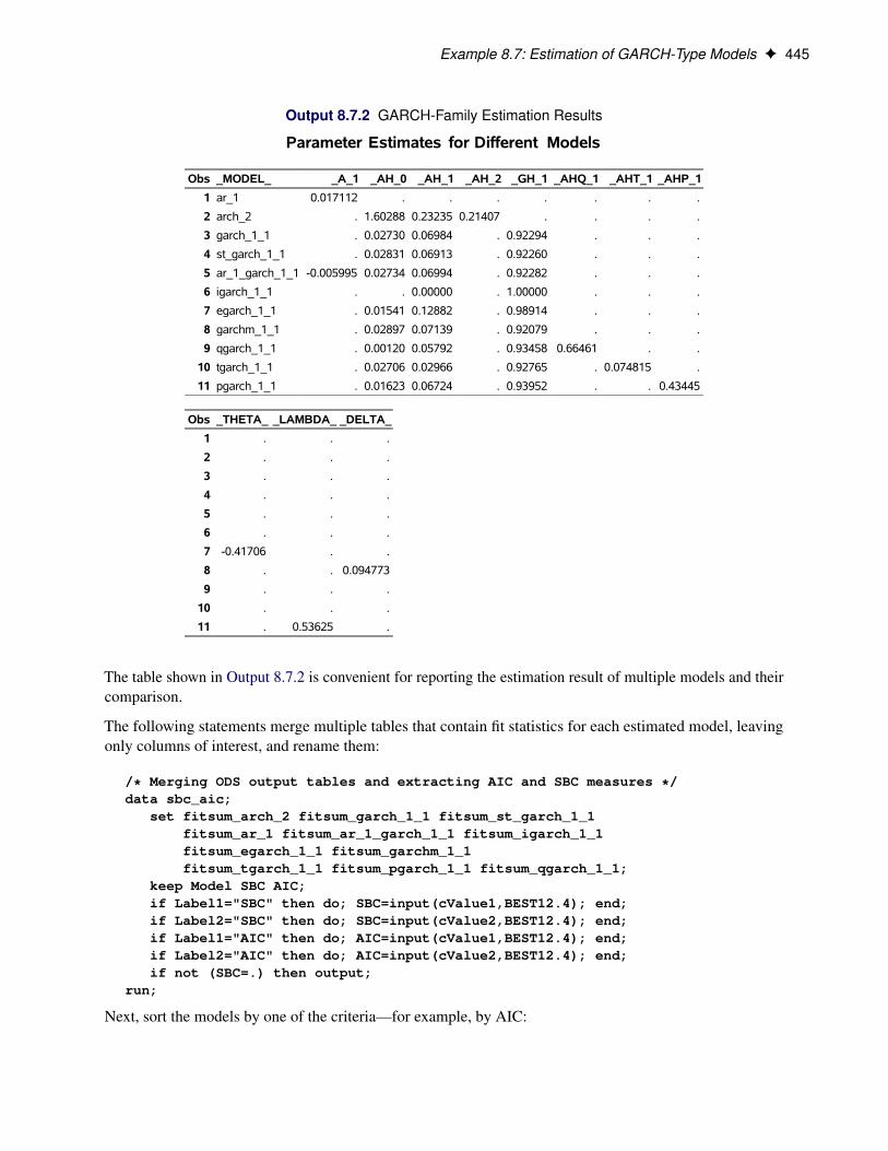
Example 8.7: Estimation of GARCH-Type Models F 445
Output 8.7.2 GARCH-Family Estimation Results
Parameter Estimates for Different Models
Obs _MODEL_ _A_1 _AH_0 _AH_1 _AH_2 _GH_1 _AHQ_1 _AHT_1 _AHP_1
1 ar_1 0.017112 . . . . . . .
2 arch_2 . 1.60288 0.23235 0.21407 . . . .
3 garch_1_1 . 0.02730 0.06984 . 0.92294 . . .
4 st_garch_1_1 . 0.02831 0.06913 . 0.92260 . . .
5 ar_1_garch_1_1 -0.005995 0.02734 0.06994 . 0.92282 . . .
6 igarch_1_1 . . 0.00000 . 1.00000 . . .
7 egarch_1_1 . 0.01541 0.12882 . 0.98914 . . .
8 garchm_1_1 . 0.02897 0.07139 . 0.92079 . . .
9 qgarch_1_1 . 0.00120 0.05792 . 0.93458 0.66461 . .
10 tgarch_1_1 . 0.02706 0.02966 . 0.92765 . 0.074815 .
11 pgarch_1_1 . 0.01623 0.06724 . 0.93952 . . 0.43445
Obs _THETA_ _LAMBDA_ _DELTA_
1 . . .
2 . . .
3 . . .
4 . . .
5 . . .
6 . . .
7 -0.41706 . .
8 . . 0.094773
9 . . .
10 . . .
11 . 0.53625 .
The table shown in Output 8.7.2 is convenient for reporting the estimation result of multiple models and theircomparison.
The following statements merge multiple tables that contain fit statistics for each estimated model, leavingonly columns of interest, and rename them:
/* Merging ODS output tables and extracting AIC and SBC measures */data sbc_aic;
set fitsum_arch_2 fitsum_garch_1_1 fitsum_st_garch_1_1fitsum_ar_1 fitsum_ar_1_garch_1_1 fitsum_igarch_1_1fitsum_egarch_1_1 fitsum_garchm_1_1fitsum_tgarch_1_1 fitsum_pgarch_1_1 fitsum_qgarch_1_1;
keep Model SBC AIC;if Label1="SBC" then do; SBC=input(cValue1,BEST12.4); end;if Label2="SBC" then do; SBC=input(cValue2,BEST12.4); end;if Label1="AIC" then do; AIC=input(cValue1,BEST12.4); end;if Label2="AIC" then do; AIC=input(cValue2,BEST12.4); end;if not (SBC=.) then output;
run;
Next, sort the models by one of the criteria—for example, by AIC:

446 F Chapter 8: The AUTOREG Procedure
/* Sorting data by AIC criterion */proc sort data=sbc_aic;
by AIC;run;
Finally, print the sorted data set:
title "Selection Criteria for Different Models";proc print data=sbc_aic;
format _NUMERIC_ BEST12.4;run;title;
The result is given in Output 8.7.3.
Output 8.7.3 GARCH-Family Model Selection on the Basis of AIC and SBC
Selection Criteria for Different Models
Obs Model SBC AIC
1 pgarch_1_1 42907.7292 42870.7722
2 egarch_1_1 42905.9616 42876.3959
3 tgarch_1_1 42995.4893 42965.9236
4 qgarch_1_1 43023.106 42993.5404
5 garchm_1_1 43158.4139 43128.8483
6 garch_1_1 43176.5074 43154.3332
7 ar_1_garch_1_1 43185.5226 43155.957
8 st_garch_1_1 43178.2497 43156.0755
9 arch_2 44605.4332 44583.259
10 ar_1 45922.0721 45914.6807
11 igarch_1_1 45925.5828 45918.1914
According to the smaller-is-better rule for the information criteria, the PGARCH(1,1) model is the leader byAIC while the EGARCH(1,1) is the model of choice according to SBC.
Next, check whether the power GARCH model is misspecified, especially, if dependence exists in thestandardized residuals that correspond to the assumed independently and identically distributed (iid) distur-bance. The following statements reestimate the power GARCH model and use the BDS test to check theindependence of the standardized residuals:
proc autoreg data=ibm_long;model r = / noint garch=(p=1,q=1,type=pgarch) BDS=(Z=SR,D=2.0);
run;
The partial results listing of the preceding statements is given in Output 8.7.4.
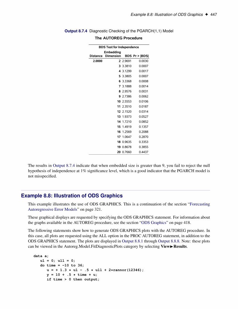
Example 8.8: Illustration of ODS Graphics F 447
Output 8.7.4 Diagnostic Checking of the PGARCH(1,1) Model
The AUTOREG Procedure
BDS Test for Independence
DistanceEmbeddingDimension BDS Pr > |BDS|
2.0000 2 2.9691 0.0030
3 3.3810 0.0007
4 3.1299 0.0017
5 3.3805 0.0007
6 3.3368 0.0008
7 3.1888 0.0014
8 2.9576 0.0031
9 2.7386 0.0062
10 2.5553 0.0106
11 2.3510 0.0187
12 2.1520 0.0314
13 1.9373 0.0527
14 1.7210 0.0852
15 1.4919 0.1357
16 1.2569 0.2088
17 1.0647 0.2870
18 0.9635 0.3353
19 0.8678 0.3855
20 0.7660 0.4437
The results in Output 8.7.4 indicate that when embedded size is greater than 9, you fail to reject the nullhypothesis of independence at 1% significance level, which is a good indicator that the PGARCH model isnot misspecified.
Example 8.8: Illustration of ODS GraphicsThis example illustrates the use of ODS GRAPHICS. This is a continuation of the section “ForecastingAutoregressive Error Models” on page 321.
These graphical displays are requested by specifying the ODS GRAPHICS statement. For information aboutthe graphs available in the AUTOREG procedure, see the section “ODS Graphics” on page 418.
The following statements show how to generate ODS GRAPHICS plots with the AUTOREG procedure. Inthis case, all plots are requested using the ALL option in the PROC AUTOREG statement, in addition to theODS GRAPHICS statement. The plots are displayed in Output 8.8.1 through Output 8.8.8. Note: these plotscan be viewed in the Autoreg.Model.FitDiagnosticPlots category by selecting ViewIResults.
data a;ul = 0; ull = 0;do time = -10 to 36;
u = + 1.3 * ul - .5 * ull + 2*rannor(12346);y = 10 + .5 * time + u;if time > 0 then output;
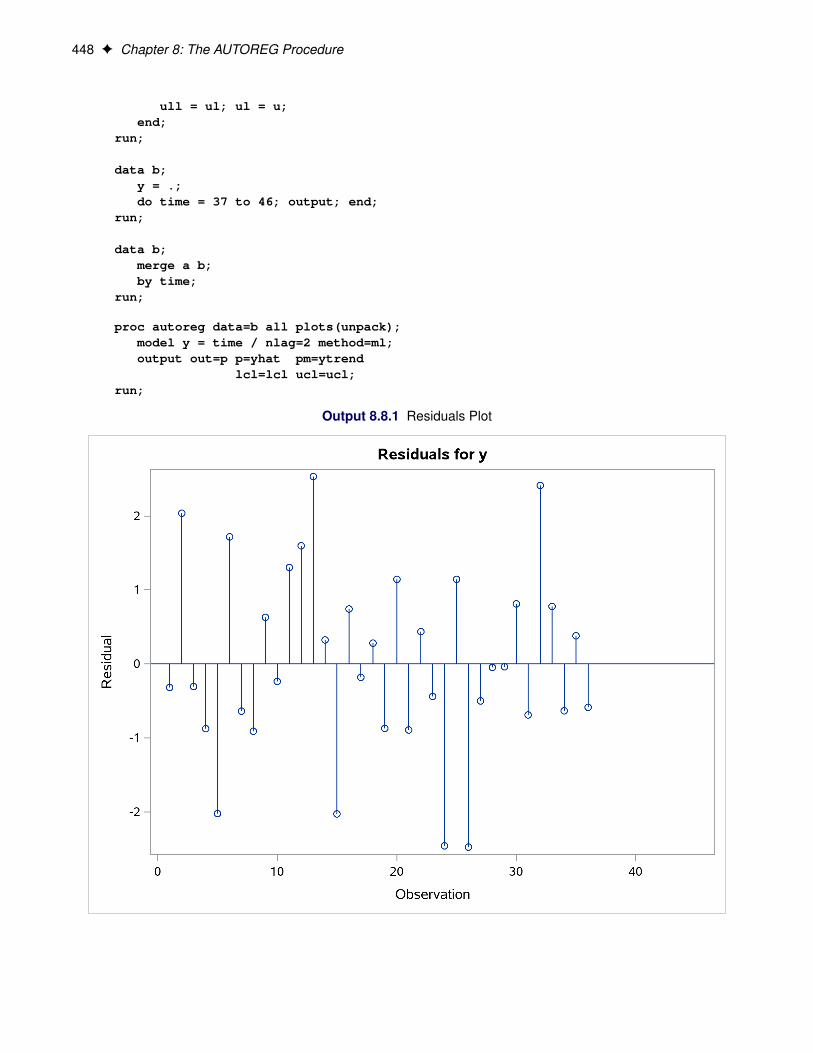
448 F Chapter 8: The AUTOREG Procedure
ull = ul; ul = u;end;
run;
data b;y = .;do time = 37 to 46; output; end;
run;
data b;merge a b;by time;
run;
proc autoreg data=b all plots(unpack);model y = time / nlag=2 method=ml;output out=p p=yhat pm=ytrend
lcl=lcl ucl=ucl;run;
Output 8.8.1 Residuals Plot

Example 8.8: Illustration of ODS Graphics F 449
Output 8.8.2 Predicted versus Actual Plot
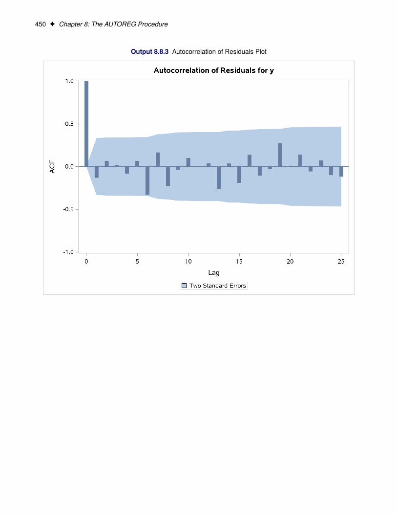
450 F Chapter 8: The AUTOREG Procedure
Output 8.8.3 Autocorrelation of Residuals Plot
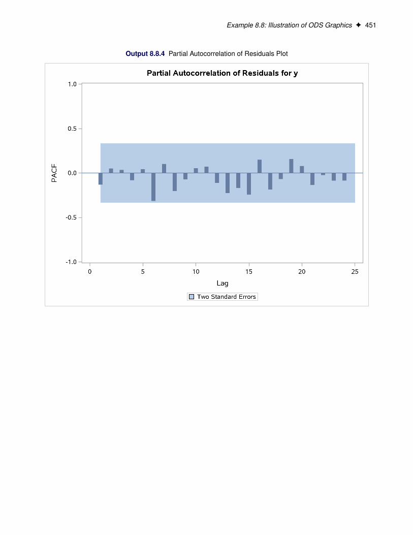
Example 8.8: Illustration of ODS Graphics F 451
Output 8.8.4 Partial Autocorrelation of Residuals Plot
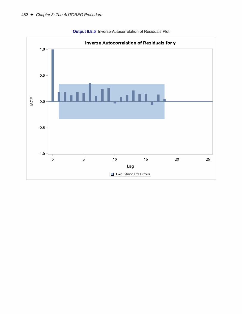
452 F Chapter 8: The AUTOREG Procedure
Output 8.8.5 Inverse Autocorrelation of Residuals Plot

Example 8.8: Illustration of ODS Graphics F 453
Output 8.8.6 Tests for White Noise Residuals Plot

454 F Chapter 8: The AUTOREG Procedure
Output 8.8.7 Q-Q Plot of Residuals
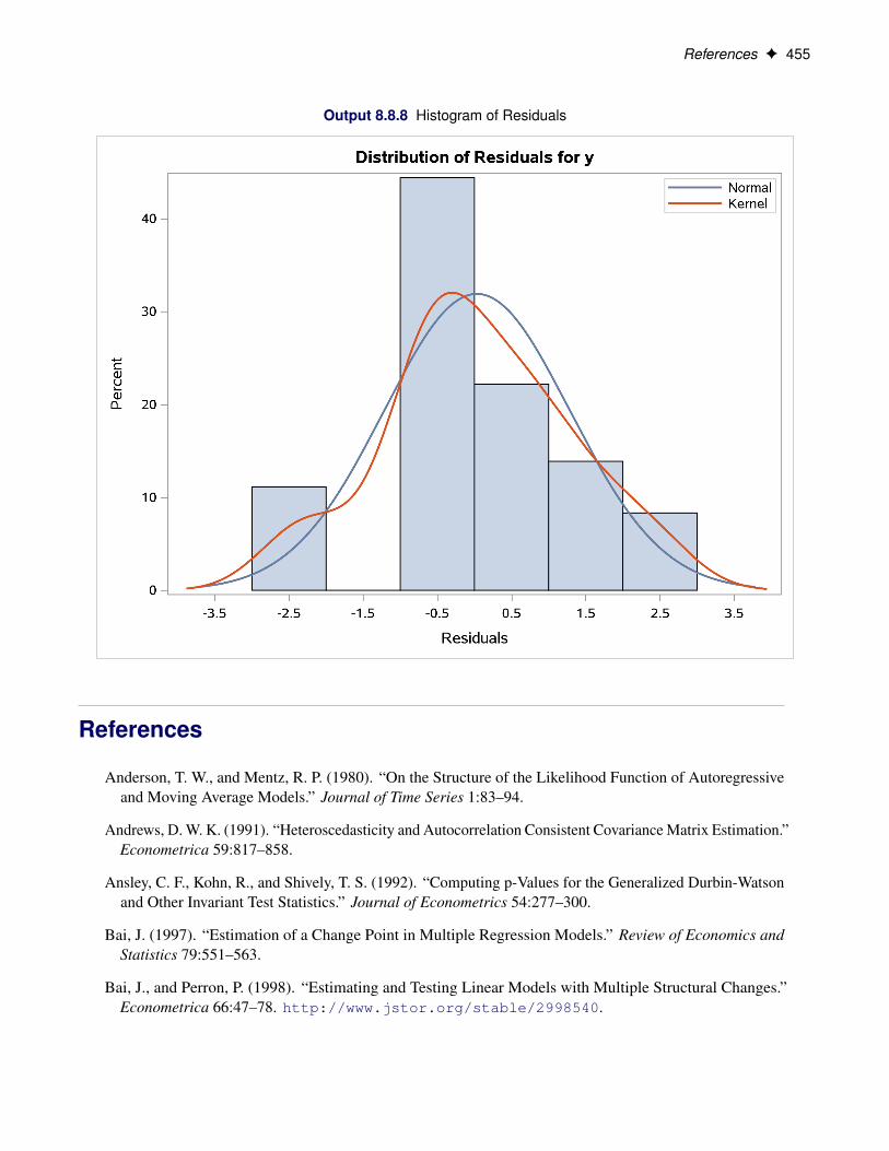
References F 455
Output 8.8.8 Histogram of Residuals
References
Anderson, T. W., and Mentz, R. P. (1980). “On the Structure of the Likelihood Function of Autoregressiveand Moving Average Models.” Journal of Time Series 1:83–94.
Andrews, D. W. K. (1991). “Heteroscedasticity and Autocorrelation Consistent Covariance Matrix Estimation.”Econometrica 59:817–858.
Ansley, C. F., Kohn, R., and Shively, T. S. (1992). “Computing p-Values for the Generalized Durbin-Watsonand Other Invariant Test Statistics.” Journal of Econometrics 54:277–300.
Bai, J. (1997). “Estimation of a Change Point in Multiple Regression Models.” Review of Economics andStatistics 79:551–563.
Bai, J., and Perron, P. (1998). “Estimating and Testing Linear Models with Multiple Structural Changes.”Econometrica 66:47–78. http://www.jstor.org/stable/2998540.

456 F Chapter 8: The AUTOREG Procedure
Bai, J., and Perron, P. (2003a). “Computation and Analysis of Multiple Structural Change Models.” Journalof Applied Econometrics 18:1–22. http://dx.doi.org/10.1002/jae.659.
Bai, J., and Perron, P. (2003b). “Critical Values for Multiple Structural Change Tests.” Econometrics Journal6:72–78. http://dx.doi.org/10.1111/1368-423X.00102.
Bai, J., and Perron, P. (2006). “Multiple Structural Change Models: A Simulation Analysis.” In EconometricTheory and Practice: Frontiers of Analysis and Applied Research, edited by D. Corbae, S. N. Durlauf, andB. E. Hansen, 212–237. Cambridge: Cambridge University Press.
Baillie, R. T. (1979). “The Asymptotic Mean Squared Error of Multistep Prediction from the RegressionModel with Autoregressive Errors.” Journal of the American Statistical Association 74:175–184.
Baillie, R. T., and Bollerslev, T. (1992). “Prediction in Dynamic Models with Time-Dependent ConditionalVariances.” Journal of Econometrics 52:91–113.
Balke, N. S., and Gordon, R. J. (1986). “Historical Data.” In The American Business Cycle, edited by R. J.Gordon, 781–850. Chicago: University of Chicago Press.
Bartels, R. (1982). “The Rank Version of von Neumann’s Ratio Test for Randomness.” Journal of theAmerican Statistical Association 77:40–46.
Beach, C. M., and MacKinnon, J. G. (1978). “A Maximum Likelihood Procedure for Regression withAutocorrelated Errors.” Econometrica 46:51–58.
Bhargava, A. (1986). “On the Theory of Testing for Unit Roots in Observed Time Series.” Review ofEconomic Studies 53:369–384.
Bollerslev, T. (1986). “Generalized Autoregressive Conditional Heteroskedasticity.” Journal of Econometrics31:307–327.
Bollerslev, T. (1987). “A Conditionally Heteroskedastic Time Series Model for Speculative Prices and Ratesof Return.” Review of Economics and Statistics 69:542–547.
Box, G. E. P., and Jenkins, G. M. (1976). Time Series Analysis: Forecasting and Control. Rev. ed. SanFrancisco: Holden-Day.
Breitung, J. (1995). “Modified Stationarity Tests with Improved Power in Small Samples.” Statistical Papers36:77–95.
Breusch, T. S., and Pagan, A. R. (1979). “A Simple Test for Heteroscedasticity and Random CoefficientVariation.” Econometrica 47:1287–1294.
Brock, W. A., Dechert, W. D., and Scheinkman, J. A. (1987). “A Test for Independence Based on theCorrelation Dimension.” Departments of Economics, University of Wisconsin–Madison, University ofHouston, and University of Chicago.
Brock, W. A., Scheinkman, J. A., Dechert, W. D., and LeBaron, B. (1996). “A Test for Independence Basedon the Correlation Dimension.” Econometric Reviews 15:197–235.
Campbell, J. Y., and Perron, P. (1991). “Pitfalls and Opportunities: What Macroeconomists Should Knowabout Unit Roots.” In NBER Macroeconomics Annual, edited by O. Blanchard and S. Fisher, 141–201.Cambridge, MA: MIT Press.

References F 457
Caner, M., and Kilian, L. (2001). “Size Distortions of Tests of the Null Hypothesis of Stationarity: Evidenceand Implications for the PPP Debate.” Journal of International Money and Finance 20:639–657.
Chipman, J. S. (1979). “Efficiency of Least Squares Estimation of Linear Trend When Residuals AreAutocorrelated.” Econometrica 47:115–128.
Chow, G. (1960). “Tests of Equality between Sets of Coefficients in Two Linear Regressions.” Econometrica28:531–534.
Cochrane, D., and Orcutt, G. H. (1949). “Application of Least Squares Regression to Relationships ContainingAutocorrelated Error Terms.” Journal of the American Statistical Association 44:32–61.
Cribari-Neto, F. (2004). “Asymptotic Inference under Heteroskedasticity of Unknown Form.” ComputationalStatistics and Data Analysis 45:215–233.
Cromwell, J. B., Labys, W. C., and Terraza, M. (1994). Univariate Tests for Time Series Models. ThousandOaks, CA: Sage Publications.
Davidson, R., and MacKinnon, J. G. (1993). Estimation and Inference in Econometrics. New York: OxfordUniversity Press.
Davies, R. B. (1973). “Numerical Inversion of a Characteristic Function.” Biometrika 60:415–417.
DeJong, D. N., Nankervis, J. C., Savin, N. E., and Whiteman, C. H. (1992). “The Power Problems of UnitRoot Rest in Time Series with Autoregressive Errors.” Journal of Econometrics 53:323–343.
Dickey, D. A., and Fuller, W. A. (1979). “Distribution of the Estimators for Autoregressive Time Series witha Unit Root.” Journal of the American Statistical Association 74:427–431.
Ding, Z., Granger, C. W. J., and Engle, R. F. (1993). “A Long Memory Property of Stock Market Returnsand a New Model.” Journal of Empirical Finance 1:83–106.
Duffie, D. (1989). Futures Markets. Englewood Cliffs, NJ: Prentice-Hall.
Durbin, J. (1969). “Tests for Serial Correlation in Regression Analysis Based on the Periodogram ofLeast-Squares Residuals.” Biometrika 56:1–15.
Durbin, J. (1970). “Testing for Serial Correlation in Least-Squares Regression When Some of the RegressorsAre Lagged Dependent Variables.” Econometrica 38:410–421.
Edgerton, D., and Wells, C. (1994). “Critical Values for the CUSUMSQ Statistic in Medium and Large SizedSamples.” Oxford Bulletin of Economics and Statistics 56:355–365.
Elliott, G., Rothenberg, T. J., and Stock, J. H. (1996). “Efficient Tests for an Autoregressive Unit Root.”Econometrica 64:813–836.
Engle, R. F. (1982). “Autoregressive Conditional Heteroscedasticity with Estimates of the Variance of UnitedKingdom Inflation.” Econometrica 50:987–1007.
Engle, R. F., and Bollerslev, T. (1986). “Modelling the Persistence of Conditional Variances.” EconometricReviews 5:1–50.
Engle, R. F., and Granger, C. W. J. (1987). “Co-integration and Error Correction: Representation, Estimation,and Testing.” Econometrica 55:251–276.

458 F Chapter 8: The AUTOREG Procedure
Engle, R. F., Lilien, D. M., and Robins, R. P. (1987). “Estimating Time Varying Risk in the Term Structure:The ARCH-M Model.” Econometrica 55:391–407.
Engle, R. F., and Ng, V. K. (1993). “Measuring and Testing the Impact of News on Volatility.” Journal ofFinance 48:1749–1778.
Engle, R. F., and Yoo, B. S. (1987). “Forecasting and Testing in Co-integrated Systems.” Journal ofEconometrics 35:143–159.
Fuller, W. A. (1976). Introduction to Statistical Time Series. New York: John Wiley & Sons.
Gallant, A. R., and Goebel, J. J. (1976). “Nonlinear Regression with Autoregressive Errors.” Journal of theAmerican Statistical Association 71:961–967.
Glosten, L., Jaganathan, R., and Runkle, D. (1993). “Relationship between the Expected Value and Volatilityof the Nominal Excess Returns on Stocks.” Journal of Finance 48:1779–1802.
Godfrey, L. G. (1978a). “Testing against General Autoregressive and Moving Average Error Models Whenthe Regressors Include Lagged Dependent Variables.” Econometrica 46:1293–1301.
Godfrey, L. G. (1978b). “Testing for Higher Order Serial Correlation in Regression Equations When theRegressors Include Lagged Dependent Variables.” Econometrica 46:1303–1310.
Godfrey, L. G. (1988). Misspecification Tests in Econometrics. Cambridge: Cambridge University Press.
Golub, G. H., and Van Loan, C. F. (1989). Matrix Computations. 2nd ed. Baltimore: Johns HopkinsUniversity Press.
Greene, W. H. (1993). Econometric Analysis. 2nd ed. New York: Macmillan.
Hamilton, J. D. (1994). Time Series Analysis. Princeton, NJ: Princeton University Press.
Hannan, E. J., and Quinn, B. G. (1979). “The Determination of the Order of an Autoregression.” Journal ofthe Royal Statistical Society, Series B 41:190–195.
Harvey, A. C. (1981). The Econometric Analysis of Time Series. New York: John Wiley & Sons.
Harvey, A. C. (1990). The Econometric Analysis of Time Series. 2nd ed. Cambridge, MA: MIT Press.
Harvey, A. C., and McAvinchey, I. D. (1978). “The Small Sample Efficiency of Two-Step Estimators inRegression Models with Autoregressive Disturbances.” Discussion Paper No. 78-10, University of BritishColumbia.
Harvey, A. C., and Phillips, G. D. A. (1979). “Maximum Likelihood Estimation of Regression Models withAutoregressive–Moving Average Disturbances.” Biometrika 66:49–58.
Hayashi, F. (2000). Econometrics. Princeton, NJ: Princeton University Press.
Hildreth, C., and Lu, J. Y. (1960). Demand Relations with Autocorrelated Disturbances. Technical Report276, Michigan State University Agricultural Experiment Station.
Hobijn, B., Franses, P. H., and Ooms, M. (2004). “Generalization of the KPSS-Test for Stationarity.” StatisticaNeerlandica 58:483–502.
References F 459
Hurvich, C. M., and Tsai, C.-L. (1989). “Regression and Time Series Model Selection in Small Samples.”Biometrika 76:297–307.
Inder, B. A. (1984). “Finite-Sample Power of Tests for Autocorrelation in Models Containing LaggedDependent Variables.” Economics Letters 14:179–185.
Inder, B. A. (1986). “An Approximation to the Null Distribution of the Durbin-Watson Statistic in ModelsContaining Lagged Dependent Variables.” Econometric Theory 2:413–428.
Jarque, C. M., and Bera, A. K. (1980). “Efficient Tests for Normality, Homoskedasticity, and SerialIndependence of Regression Residuals.” Economics Letters 6:255–259.
Johansen, S. (1988). “Statistical Analysis of Cointegration Vectors.” Journal of Economic Dynamics andControl 12:231–254.
Johansen, S. (1991). “Estimation and Hypothesis Testing of Cointegration Vectors in Gaussian VectorAutoregressive Models.” Econometrica 59:1551–1580.
Johnston, J. (1972). Econometric Methods. 2nd ed. New York: McGraw-Hill.
Jones, R. H. (1980). “Maximum Likelihood Fitting of ARMA Models to Time Series with MissingObservations.” Technometrics 22:389–396.
Judge, G. G., Griffiths, W. E., Hill, R. C., Lütkepohl, H., and Lee, T.-C. (1985). The Theory and Practice ofEconometrics. 2nd ed. New York: John Wiley & Sons.
Kanzler, L. (1999). “Very Fast and Correctly Sized Estimation of the BDS Statistic.” Working paper,Department of Economics, Christ Church, University of Oxford.
King, M. L., and Wu, P. X. (1991). “Small-Disturbance Asymptotics and the Durbin-Watson and RelatedTests in the Dynamic Regression Model.” Journal of Econometrics 47:145–152.
Kwiatkowski, D., Phillips, P. C. B., Schmidt, P., and Shin, Y. (1992). “Testing the Null Hypothesis ofStationarity against the Alternative of a Unit Root.” Journal of Econometrics 54:159–178.
LaMotte, L. R. (1994). “A Note on the Role of Independence in t Statistics Constructed from Linear Statisticsin Regression Models.” American Statistician 48:238–240.
Lee, J. H., and King, M. L. (1993). “A Locally Most Mean Powerful Based Score Test for ARCH andGARCH Regression Disturbances.” Journal of Business and Economic Statistics 11:17–27.
L’Esperance, W. L., Chall, D., and Taylor, D. (1976). “An Algorithm for Determining the DistributionFunction of the Durbin-Watson Test Statistic.” Econometrica 44:1325–1326.
MacKinnon, J. G. (1991). “Critical Values for Cointegration Tests.” In Long-Run Economic Relationships:Readings in Cointegration, edited by R. F. Engle and C. W. J. Granger, 267–276. Oxford: Oxford UniversityPress.
Maddala, G. S. (1977). Econometrics. New York: McGraw-Hill.
Maeshiro, A. (1976). “Autoregressive Transformation, Trended Independent Variables and AutocorrelatedDisturbance Terms.” Review of Economics and Statistics 58:497–500.
460 F Chapter 8: The AUTOREG Procedure
McLeod, A. I., and Li, W. K. (1983). “Diagnostic Checking ARMA Time Series Models Using Squared-Residual Autocorrelations.” Journal of Time Series Analysis 4:269–273.
Nelson, C. R., and Plosser, C. I. (1982). “Trends and Random Walks in Macroeconomic Time Series: SomeEvidence and Implications.” Journal of Monetary Economics 10:139–162.
Nelson, D. B. (1990). “Stationarity and Persistence in the GARCH(1,1) Model.” Econometric Theory6:318–334.
Nelson, D. B. (1991). “Conditional Heteroskedasticity in Asset Returns: A New Approach.” Econometrica59:347–370.
Nelson, D. B., and Cao, C. Q. (1992). “Inequality Constraints in the Univariate GARCH Model.” Journal ofBusiness and Economic Statistics 10:229–235.
Newey, W. K., and West, D. W. (1987). “A Simple, Positive Semi-definite, Heteroskedasticity and Autocorre-lation Consistent Covariance Matrix.” Econometrica 55:703–708.
Newey, W. K., and West, D. W. (1994). “Automatic Lag Selection in Covariance Matrix Estimation.” Reviewof Economic Studies 61:631–653.
Ng, S., and Perron, P. (2001). “Lag Length Selection and the Construction of Unit Root Tests with GoodSize and Power.” Econometrica 69:1519–1554.
Park, R. E., and Mitchell, B. M. (1980). “Estimating the Autocorrelated Error Model with Trended Data.”Journal of Econometrics 13:185–201.
Phillips, P. C. B. (1987). “Time Series Regression with a Unit Root.” Econometrica 55:277–301.
Phillips, P. C. B., and Ouliaris, S. (1990). “Asymptotic Properties of Residual Based Tests for Cointegration.”Econometrica 58:165–193.
Phillips, P. C. B., and Perron, P. (1988). “Testing for a Unit Root in Time Series Regression.” Biometrika75:335–346.
Prais, S. J., and Winsten, C. B. (1954). “Trend Estimators and Serial Correlation.” Cowles CommissionDiscussion Paper No. 383.
Ramsey, J. B. (1969). “Tests for Specification Errors in Classical Linear Least Squares Regression Analysis.”Journal of the Royal Statistical Society, Series B 31:350–371.
Said, S. E., and Dickey, D. A. (1984). “Testing for Unit Roots in ARMA Models of Unknown Order.”Biometrika 71:599–607.
Savin, N. E., and White, K. J. (1978). “Testing for Autocorrelation with Missing Observations.” Econometrica46:59–67.
Schwarz, G. (1978). “Estimating the Dimension of a Model.” Annals of Statistics 6:461–464.
Schwert, G. (1989). “Tests for Unit Roots: A Monte Carlo Investigation.” Journal of Business and EconomicStatistics 7:147–159.
Shin, Y. (1994). “A Residual-Based Test of the Null of Cointegration against the Alternative of No Cointegra-tion.” Econometric Theory 10:91–115. http://dx.doi.org/10.1017/S0266466600008240.

References F 461
Shively, T. S. (1990). “Fast Evaluation of the Distribution of the Durbin-Watson and Other Invariant TestStatistics in Time Series Regression.” Journal of the American Statistical Association 85:676–685.
Spitzer, J. J. (1979). “Small-Sample Properties of Nonlinear Least Squares and Maximum LikelihoodEstimators in the Context of Autocorrelated Errors.” Journal of the American Statistical Association74:41–47.
Stock, J. H. (1994). “Unit Roots, Structural Breaks, and Trends.” In Handbook of Econometrics, edited byR. F. Engle and D. L. McFadden, 2739–2841. Amsterdam: North-Holland.
Stock, J. H., and Watson, M. W. (1988). “Testing for Common Trends.” Journal of the American StatisticalAssociation 83:1097–1107.
Stock, J. H., and Watson, M. W. (2002). Introduction to Econometrics. 3rd ed. Reading, MA: Addison-Wesley.
Theil, H. (1971). Principles of Econometrics. New York: John Wiley & Sons.
Vinod, H. D. (1973). “Generalization of the Durbin-Watson Statistic for Higher Order AutoregressiveProcess.” Communications in Statistics 2:115–144.
Wallis, K. F. (1972). “Testing for Fourth Order Autocorrelation in Quarterly Regression Equations.” Econo-metrica 40:617–636.
White, H. (1980). “A Heteroskedasticity-Consistent Covariance Matrix Estimator and a Direct Test forHeteroskedasticity.” Econometrica 48:817–838.
White, H. (1982). “Maximum Likelihood Estimation of Misspecified Models.” Econometrica 50:1–25.
White, K. J. (1992). “The Durbin-Watson Test for Autocorrelation in Nonlinear Models.” Review ofEconomics and Statistics 74:370–373.
Wong, H., and Li, W. K. (1995). “Portmanteau Test for Conditional Heteroscedasticity, Using Ranks ofSquared Residuals.” Journal of Applied Statistics 22:121–134.
Zakoian, J. M. (1994). “Threshold Heteroscedastic Models.” Journal of Economic Dynamics and Control18:931–955.
Subject Index
ADF test, 353Akaike’s information criterion
AUTOREG procedure, 384Akaike’s information criterion corrected
AUTOREG procedure, 384ARCH model
AUTOREG procedure, 313autoregressive conditional heteroscedasticity, 313
augmented Dickey-Fuller (ADF) test, 353autocorrelation tests
Durbin-Watson test, 351Godfrey’s test, 351
AUTOREG procedureAkaike’s information criterion, 384Akaike’s information criterion corrected, 384ARCH model, 313autoregressive error correction, 314BY groups, 340Cholesky root, 371Cochrane-Orcutt method, 372conditional variance, 411confidence limits, 364dual quasi-Newton method, 379Durbin h test, 324Durbin t test, 324Durbin-Watson test, 322EGARCH model, 334EGLS method, 372estimation methods, 369factored model, 326GARCH model, 313GARCH-M model, 334Gauss-Marquardt method, 371generalized Durbin-Watson tests, 322Hannan-Quinn information criterion, 384heteroscedasticity, 327Hildreth-Lu method, 373IGARCH model, 334Kalman filter, 371lagged dependent variables, 324maximum likelihood method, 373nonlinear least-squares, 372ODS graph names, 418output data sets, 413output table names, 416PGARCH model, 334Prais-Winsten estimates, 372predicted values, 364, 409, 410
printed output, 415QGARCH model, 334quasi-Newton method, 343random walk model, 427residuals, 365Schwarz Bayesian criterion, 384serial correlation correction, 314stepwise autoregression, 325structural predictions, 409subset model, 326TGARCH model, 334Toeplitz matrix, 369trust region method, 343two-step full transform method, 372Yule-Walker equations, 369Yule-Walker estimates, 369
autoregressive conditional heteroscedasticity, seeARCH model
autoregressive error correctionAUTOREG procedure, 314
Bai and Perron’s multiple structural change tests, 406BDS test, 344, 397
for independence, 344BP test, 345
for structural change, 345BY groups
AUTOREG procedure, 340
Cholesky rootAUTOREG procedure, 371
Chow test, 348, 352, 405for structural change, 348
Cochrane-Orcutt methodAUTOREG procedure, 372
cointegration test, 356, 391conditional t distribution
GARCH model, 378conditional variance
AUTOREG procedure, 411predicted values, 411predicting, 411
confidence limitsAUTOREG procedure, 364
constrained estimationheteroscedasticity models, 362
covariance estimatesGARCH model, 349
covariates
heteroscedasticity models, 360CUSUM statistics, 364, 383
dual quasi-Newton methodAUTOREG procedure, 379
Durbin h testAUTOREG procedure, 324
Durbin t testAUTOREG procedure, 324
Durbin-Watson testautocorrelation tests, 351AUTOREG procedure, 322for first-order autocorrelation, 322for higher-order autocorrelation, 322p-values for, 322
Durbin-Watson tests, 351linearized form, 360
EGARCH modelAUTOREG procedure, 334
EGLS methodAUTOREG procedure, 372
Engle’s Lagrange multiplier test, 404for heteroscedasticity, 404
estimation methodsAUTOREG procedure, 369
factored modelAUTOREG procedure, 326
first-order autocorrelationDurbin-Watson test for, 322
GARCH in mean model, see GARCH-M modelGARCH model
AUTOREG procedure, 313conditional t distribution, 378covariance estimates, 349generalized autoregressive conditional
heteroscedasticity, 313heteroscedasticity models, 360initial values, 359starting values, 343t distribution, 378
GARCH-M model, 378AUTOREG procedure, 334GARCH in mean model, 378
Gauss-Marquardt methodAUTOREG procedure, 371
generalized autoregressive conditionalheteroscedasticity, see GARCH model
generalized Durbin-Watson testsAUTOREG procedure, 322
generalized least squaresYule-Walker method as, 372
Godfrey’s test, 351
autocorrelation tests, 351
Hannan-Quinn information criterionAUTOREG procedure, 384
heteroscedasticityAUTOREG procedure, 327Engle’s Lagrange multiplier test for, 404Lagrange multiplier test, 362Lee and King’s test for, 404portmanteau Q test for, 403testing for, 327Wong and Li’s test for, 405
heteroscedasticity models, see GARCH modelconstrained estimation, 362covariates, 360link function, 361
heteroscedasticity testsLagrange multiplier test, 362
higher-order autocorrelationDurbin-Watson test for, 322
Hildreth-Lu methodAUTOREG procedure, 373
IGARCH modelAUTOREG procedure, 334
independenceBDS test for, 344, 397rank version of von Neumann ratio test for, 358,
399runs test for, 353, 398turning point test for, 357, 398
initial values, 359GARCH model, 359
Jarque-Bera test, 352normality tests, 352
Kalman filterAUTOREG procedure, 371
KPSS (Kwiatkowski, Phillips, Schmidt, Shin) test, 354KPSS test, 354, 394
unit roots, 354, 394
lagged dependent variablesand tests for autocorrelation, 324AUTOREG procedure, 324
Lagrange multiplier testheteroscedasticity, 362heteroscedasticity tests, 362
Lee and King’s test, 404for heteroscedasticity, 404
linearized formDurbin-Watson tests, 360
link functionheteroscedasticity models, 361
log-likelihood value, 352
MAEAUTOREG procedure, 383
MAPEAUTOREG procedure, 383
maximum likelihood methodAUTOREG procedure, 373
nonlinear least-squaresAUTOREG procedure, 372
normality testsJarque-Bera test, 352
ODS graph namesAUTOREG procedure, 418
optimization methodsquasi-Newton, 360trust region, 360
output data setsAUTOREG procedure, 413
output table namesAUTOREG procedure, 416
PGARCH model, 376AUTOREG procedure, 334power GARCH model, 376
Phillips-Ouliaris test, 356, 391Phillips-Perron test, 356, 390
unit roots, 356, 390portmanteau Q test, 403
for heteroscedasticity, 403power GARCH model, see PGARCH modelPrais-Winsten estimates
AUTOREG procedure, 372predicted values
AUTOREG procedure, 364, 409, 410conditional variance, 411structural, 364, 409
predicting conditional variance, 411predictive Chow test, 352, 406printed output
AUTOREG procedure, 415
QGARCH model, 376AUTOREG procedure, 334quadratic GARCH model, 376
quadratic GARCH model, see QGARCH modelquasi-Newton method, 360
AUTOREG procedure, 343quasi-Newton optimization methods, 360
Ramsey’s test, see RESET testrandom walk model
AUTOREG procedure, 427
rank version of von Neumann ratio test, 358, 399for independence, 399
recursive residuals, 364, 383RESET test, 352
Ramsey’s test, 352residuals
AUTOREG procedure, 365structural, 365
RESTRICT statement, 365restricted estimation, 365runs test, 353, 398
for independence, 353, 398
Schwarz Bayesian criterionAUTOREG procedure, 384
serial correlation correctionAUTOREG procedure, 314
Shin test, 354, 394unit roots, 354, 394
standard errors, 365starting values
GARCH model, 343stationarity tests, 353stepwise autoregression
AUTOREG procedure, 325structural change
BP test for, 345Chow test for, 348
structural predicted values, 364structural predictions
AUTOREG procedure, 409structural residuals, 365structural standard errors, 365subset model
AUTOREG procedure, 326
t distributionGARCH model, 378
TEST statement, 366tests for autocorrelation
lagged dependent variables and, 324tests of parameters, 366TGARCH model, 376
AUTOREG procedure, 334threshold GARCH model, 376
threshold GARCH model, see TGARCH modelToeplitz matrix
AUTOREG procedure, 369trust region
optimization methods, 360trust region method, 360
AUTOREG procedure, 343turning point test, 357, 398
for independence, 357, 398

two-step full transform methodAUTOREG procedure, 372
unit rootsKPSS test, 354, 394Phillips-Perron test, 356, 390Shin test, 354, 394
Wong and Li’s test, 405for heteroscedasticity, 405
Yule-Walker equationsAUTOREG procedure, 369
Yule-Walker estimatesAUTOREG procedure, 369
Yule-Walker methodas generalized least squares, 372

Syntax Index
ALL optionMODEL statement (AUTOREG), 343
ALPHACLI= optionOUTPUT statement (AUTOREG), 363
ALPHACLM= optionOUTPUT statement (AUTOREG), 363
ALPHACSM= optionOUTPUT statement (AUTOREG), 363
ARCHTEST optionMODEL statement (AUTOREG), 343
AUTOREG procedure, 335syntax, 335
AUTOREG procedure, AUTOREG statement, 341
BACKSTEP optionMODEL statement (AUTOREG), 358
BDS optionMODEL statement (AUTOREG), 344
BLUS= optionOUTPUT statement (AUTOREG), 363
BP optionMODEL statement (AUTOREG), 345
BY statementAUTOREG procedure, 340
CENTER optionMODEL statement (AUTOREG), 341
CEV= optionOUTPUT statement (AUTOREG), 363
CHOW= optionMODEL statement (AUTOREG), 348
COEF optionMODEL statement (AUTOREG), 349
COEF= optionHETERO statement (AUTOREG), 362
CONSTANT= optionOUTPUT statement (AUTOREG), 364
CONVERGE= optionMODEL statement (AUTOREG), 359
CORRB optionMODEL statement (AUTOREG), 349
COVB optionMODEL statement (AUTOREG), 349
COVEST= optionMODEL statement (AUTOREG), 349
COVOUT optionPROC AUTOREG statement, 339
CPEV= optionOUTPUT statement (AUTOREG), 363
CUSUM= optionOUTPUT statement (AUTOREG), 364
CUSUMLB= optionOUTPUT statement (AUTOREG), 364
CUSUMSQ= optionOUTPUT statement (AUTOREG), 364
CUSUMSQLB= optionOUTPUT statement (AUTOREG), 364
CUSUMSQUB= optionOUTPUT statement (AUTOREG), 364
CUSUMUB= optionOUTPUT statement (AUTOREG), 364
DATA= optionPROC AUTOREG statement, 339
DIST= optionMODEL statement (AUTOREG), 341
DW= optionMODEL statement (AUTOREG), 351
DWPROB optionMODEL statement (AUTOREG), 351
GARCH= optionMODEL statement (AUTOREG), 342
GINV optionMODEL statement (AUTOREG), 351
GODFREY optionMODEL statement (AUTOREG), 351
HETERO statementAUTOREG procedure, 360
HT= optionOUTPUT statement (AUTOREG), 363
INITIAL= optionMODEL statement (AUTOREG), 359
ITPRINT optionMODEL statement (AUTOREG), 351
JACOBOUT optionPROC AUTOREG statement, 339
LAGDEP optionMODEL statement (AUTOREG), 352
LAGDEP= optionMODEL statement (AUTOREG), 352
LAGDV optionMODEL statement (AUTOREG), 352
LAGDV= option

MODEL statement (AUTOREG), 352LCL= option
OUTPUT statement (AUTOREG), 364LCLM= option
OUTPUT statement (AUTOREG), 364LDW option
MODEL statement (AUTOREG), 360LINK= option
HETERO statement (AUTOREG), 361LOGLIKL option
MODEL statement (AUTOREG), 352
MAXITER= optionMODEL statement (AUTOREG), 360
MEAN= optionMODEL statement (AUTOREG), 343
METHOD= optionMODEL statement (AUTOREG), 360
MODEL statementAUTOREG procedure, 341
NLAG= optionMODEL statement (AUTOREG), 341
NLOPTIONS statementAUTOREG procedure, 362
NOCONST optionHETERO statement (AUTOREG), 362
NOINT optionMODEL statement (AUTOREG), 341, 343
NOMISS optionMODEL statement (AUTOREG), 360
NOPRINT optionMODEL statement (AUTOREG), 352
NORMAL optionMODEL statement (AUTOREG), 352
OPTMETHOD= optionMODEL statement (AUTOREG), 360
OUT= optionOUTPUT statement (AUTOREG), 363
OUTEST= optionPROC AUTOREG statement, 339
OUTPUTOUT=, 413
OUTPUT statementAUTOREG procedure, 363
P= optionMODEL statement (AUTOREG), 342OUTPUT statement (AUTOREG), 364
PARTIAL optionMODEL statement (AUTOREG), 352
PCHOW= optionMODEL statement (AUTOREG), 352
PLOTS option
PROC AUTOREG statement, 339PM= option
OUTPUT statement (AUTOREG), 364PREDICTED= option
OUTPUT statement (AUTOREG), 364PREDICTEDM= option
OUTPUT statement (AUTOREG), 364PROC AUTOREG
OUTEST=, 413PROC AUTOREG statement, 339
Q= optionMODEL statement (AUTOREG), 342
R= optionOUTPUT statement (AUTOREG), 365
RECPEV= optionOUTPUT statement (AUTOREG), 364
RECRES= optionOUTPUT statement (AUTOREG), 364
RESET optionMODEL statement (AUTOREG), 352
RESIDUAL= optionOUTPUT statement (AUTOREG), 365
RESIDUALM= optionOUTPUT statement (AUTOREG), 365
RESTRICT statementAUTOREG procedure, 365
RM= optionOUTPUT statement (AUTOREG), 365
RUNS optionMODEL statement (AUTOREG), 353
SE= optionOUTPUT statement (AUTOREG), 365
SEM= optionOUTPUT statement (AUTOREG), 365
SLSTAY= optionMODEL statement (AUTOREG), 359
START= optionMODEL statement (AUTOREG), 359
STARTUP= optionMODEL statement (AUTOREG), 343
STATIONARITY= optionMODEL statement (AUTOREG), 353
STD= optionHETERO statement (AUTOREG), 362
STDERR= optionOUTPUT statement (AUTOREG), 365
STDERRM= optionOUTPUT statement (AUTOREG), 365
TEST statementAUTOREG procedure, 366
TEST= option
HETERO statement (AUTOREG), 362TP option
MODEL statement (AUTOREG), 357TR option
MODEL statement (AUTOREG), 343TRANSFORM= option
OUTPUT statement (AUTOREG), 365TYPE= option
MODEL statement (AUTOREG), 342TEST statement (AUTOREG), 367
UCL= optionOUTPUT statement (AUTOREG), 365
UCLM= optionOUTPUT statement (AUTOREG), 365
URSQ optionMODEL statement (AUTOREG), 357
VNRRANK optionMODEL statement (AUTOREG), 358