University:

Kennesaw State University

Team Members:

1) Alex Tatum

2) Bogdan Gadidov

3) Breana Murphy

4) John Croft

5) Kate Phillips

6) Kayon Hines

7) Meaghan Bruce

8) Mike Smothers

Supporting Faculty Member:

1) Sherry Ni

Primary Contact:

Sherry Ni

Email: xni2@kennesaw.edu

Team Number:

52

Date Submitted:

June 3rd

, 2014

Team Number: 52

Page 1 of 33

EXECUTIVE SUMMARY

As population density increases, and socioeconomic factors trend downward, increasing crime

rates become a major concern for our country. This paper analyzes how to allocate police

resources to minimize the crime rate throughout the target cities. The provided analysis brings to

light new evidence on crime trends were possibly missed with previous statistical methods. This

analysis will help determine how to cross train the police force effectively to respond to specific

crimes and an overall increasing crime rate.

1 PROBLEM DEFINITION

In the initial stage of the analysis, in order to achieve the

objectives, current societal norms and preliminary project plans

are established.

Lowering crime rates and keeping police forces in line with future predictable natural

phenomena is of particular interest to the law enforcement community. The lowering of crime

rates are also important to those that support or pay for those enforcement activities. “Statistics

released in the FBI’s Preliminary Semiannual Uniform Crime Report reveal declines in both the

violent crime and the property crime reported in the first six months of 2013 when compared

with figures for the first six months of 2012. The report has information from 12,723 law

enforcement agencies that submitted three to six months of comparable data to the FBI Uniform

Crime Reporting (UCR) Program for the first six months of 2012 and 2013” (James B. Comey,

2013). Improving crime prediction accuracy could improve the above referenced FBI statistics

and improve the quality of life for those affected.

Other than population and socioeconomic factors, multiple studies have explored additional

predictors of crimes in specific areas. Prior studies imply that the availability of light may affect

the amount and types of crimes committed. The significance of daylight savings time is currently

being evaluated. It is hypothesized that more daylight results in less crime. (Sanders, 2012)

E.G. Cohn discussed weather and temporal variations (time of day, day of week, holidays, etc.)

during requests for police services (Cohn, 1993) and A.D. Pokorny & J. Jachimczyk used phases

of the moon as a possible predictor to explore the relationship between homicides and the lunar

cycle. (A.D. Pokorny, 1974)

Team Number: 52

Page 2 of 33

Even though these studies used data mining techniques, all of these studies attempted their

exploration with a narrow scope. They failed to take into account the broader possibilities

leading to inadequate factors that affect the frequency or type of crimes committed.

This study attempts to model crime on a broader set of possibilities to determine which factors

are significant, allowing for the most efficient police resource allocation. Utilizing the Cross

Industry Standard Process for Data Mining (CRISM-DM) model, this model breaks our task

down into six nodes: problem definition, data understanding, data preparation, modeling,

evaluation, and deployment. This allows ideas and processes to flow freely throughout the nodes

allowing progress towards a common goal.

2 DATA UNDERSTANDING

Stage two of the analysis begins with familiarization and

exploration of the provided data.

2.1 Identifying Data Quality

Of the nine provided data sets, eight were utilized; Heating_Cooling_Days was not used because

its relevant information was extracted from the other provided data sets. Of the remaining

datasets, two contained missing values. CRIME_V2 had 130 missing tract_id values; these

observations were not used because the dataset was large enough (over observations)

to compensate for the loss. Weather had one missing value each for temperature_low,

temperature_high, and pressure; for this dataset, missing values were imputed with the average

of the surrounding day’s values.

The original Population dataset did not contain any missing values; however, it only provided

data for the years 2000 and 2010. In order to provide a complete dataset that includes population

values for every year from 2005 to 2012, values were extrapolated based on the 2000 and 2010

data. Additionally, time and naming conventions used were inconsistent; therefore, values were

reformatted for consistency.

Team Number: 52

Page 3 of 33

2.2 Initial Insights

Two models, binary and numeric, were constructed to determine significant factors for crime

prediction. The binary model uses a binary response as the target. This model determines if any

crimes occurred. The binary model also targets significant factors to improve the accuracy of the

second models numerical response. The numerical model uses the numerical number of crimes

as the target, and indicates how many total crimes occurred. This model is useful in revealing the

effect of the significant factors for each type of crime. A third model was developed by taking

the numeric crime type, dividing it by the population total, and then multiplying it by 100. This

equation created a crime_ratio response variable. This model is useful in evaluating the problem

statement.

3 Data Preparation

Stage three addresses merging, variable creation, and variable

selection.

3.1 Our Process

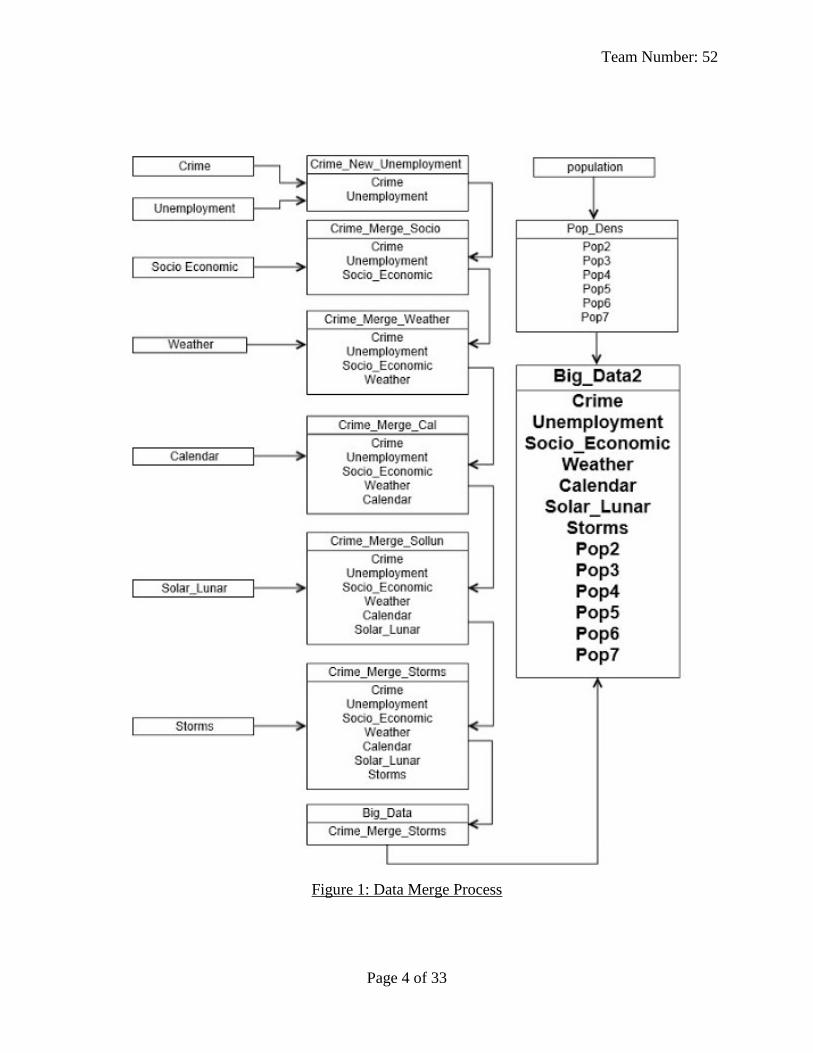
After performing data validation, the selected datasets were then merged into a single SAS file

before being uploaded into Enterprise Miner. Figure 1 below outlines how the merging was

performed.

Team Number: 52

Page 4 of 33

Figure 1: Data Merge Process

Team Number: 52

Page 5 of 33

Once the merging was completed, a data source was created in Enterprise Miner. Three separate

data models were then created. The first data model was established as the Binary set. The

binary set was modeled representing whether a crime occurred or did not occur. The second

model contained the numeric response for total crimes, which represented how many crimes

were committed per day. Finally, the third model was created which establishes the crime ratio.

The crime ratio is the crime per 100 people per day.

3.2 Data Description

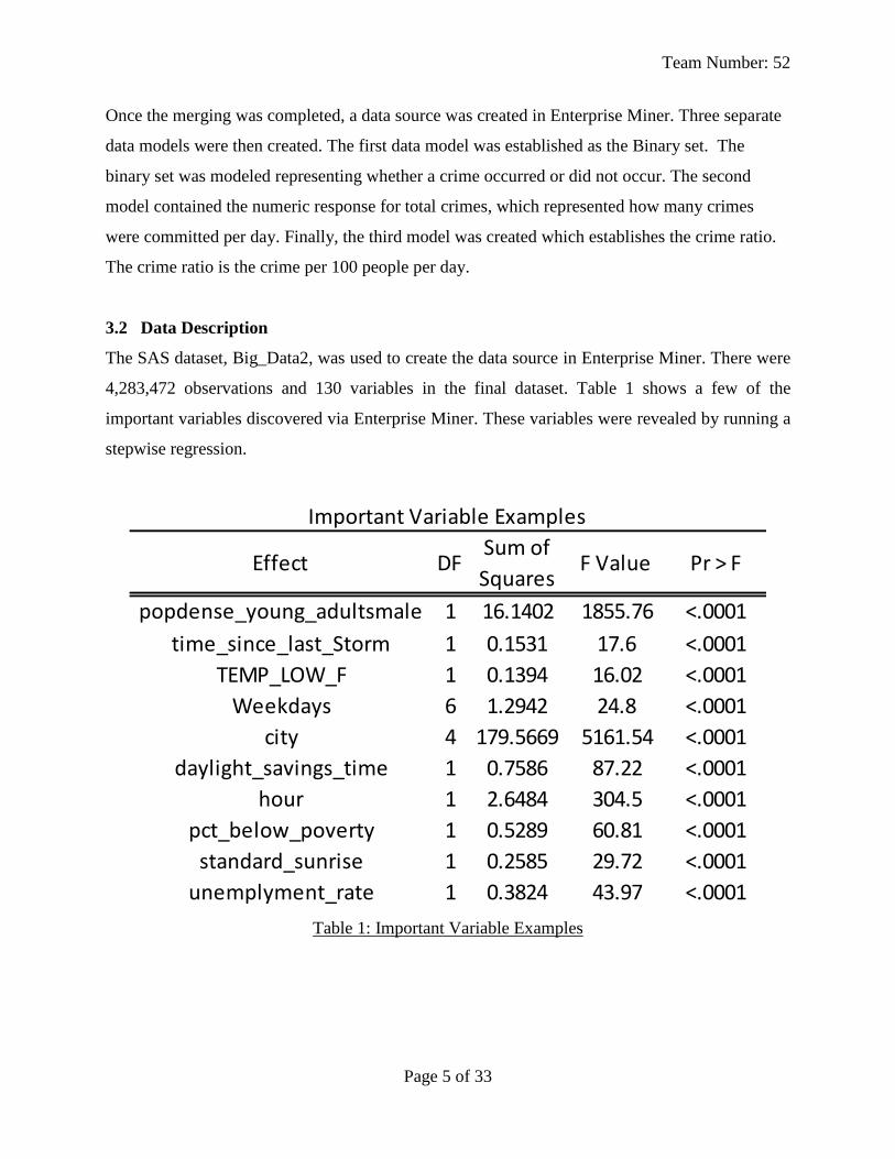
The SAS dataset, Big_Data2, was used to create the data source in Enterprise Miner. There were

4,283,472 observations and 130 variables in the final dataset. Table 1 shows a few of the

important variables discovered via Enterprise Miner. These variables were revealed by running a

stepwise regression.

Table 1: Important Variable Examples

Effect DFSum of

SquaresF Value Pr > F

popdense_young_adultsmale 1 16.1402 1855.76 <.0001

time_since_last_Storm 1 0.1531 17.6 <.0001

TEMP_LOW_F 1 0.1394 16.02 <.0001

Weekdays 6 1.2942 24.8 <.0001

city 4 179.5669 5161.54 <.0001

daylight_savings_time 1 0.7586 87.22 <.0001

hour 1 2.6484 304.5 <.0001

pct_below_poverty 1 0.5289 60.81 <.0001

standard_sunrise 1 0.2585 29.72 <.0001

unemplyment_rate 1 0.3824 43.97 <.0001

Important Variable Examples

Team Number: 52

Page 6 of 33

4 MODELING

Stage four addresses selecting several modeling techniques and

applying them to find the most important variables.

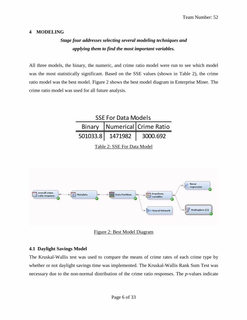
All three models, the binary, the numeric, and crime ratio model were run to see which model

was the most statistically significant. Based on the SSE values (shown in Table 2), the crime

ratio model was the best model. Figure 2 shows the best model diagram in Enterprise Miner. The

crime ratio model was used for all future analysis.

Table 2: SSE For Data Model

Figure 2: Best Model Diagram

4.1 Daylight Savings Model

The Kruskal-Wallis test was used to compare the means of crime rates of each crime type by

whether or not daylight savings time was implemented. The Kruskal-Wallis Rank Sum Test was

necessary due to the non-normal distribution of the crime ratio responses. The p-values indicate

Binary Numerical Crime Ratio

501033.8 1471982 3000.692

SSE For Data Models

Team Number: 52

Page 7 of 33

if the differences in means are significant. In general, it was discovered that crime rate increases

when daylight savings is implemented.

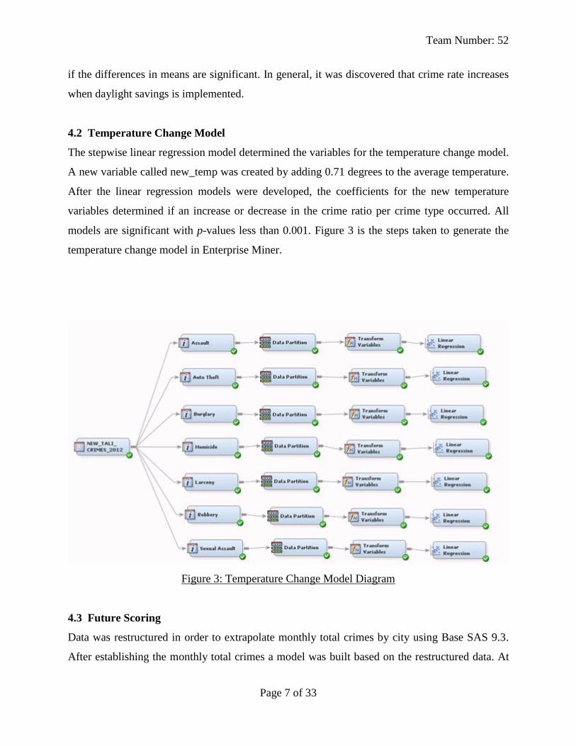
4.2 Temperature Change Model

The stepwise linear regression model determined the variables for the temperature change model.

A new variable called new_temp was created by adding 0.71 degrees to the average temperature.

After the linear regression models were developed, the coefficients for the new temperature

variables determined if an increase or decrease in the crime ratio per crime type occurred. All

models are significant with p-values less than 0.001. Figure 3 is the steps taken to generate the

temperature change model in Enterprise Miner.

Figure 3: Temperature Change Model Diagram

4.3 Future Scoring

Data was restructured in order to extrapolate monthly total crimes by city using Base SAS 9.3.

After establishing the monthly total crimes a model was built based on the restructured data. At

Team Number: 52

Page 8 of 33

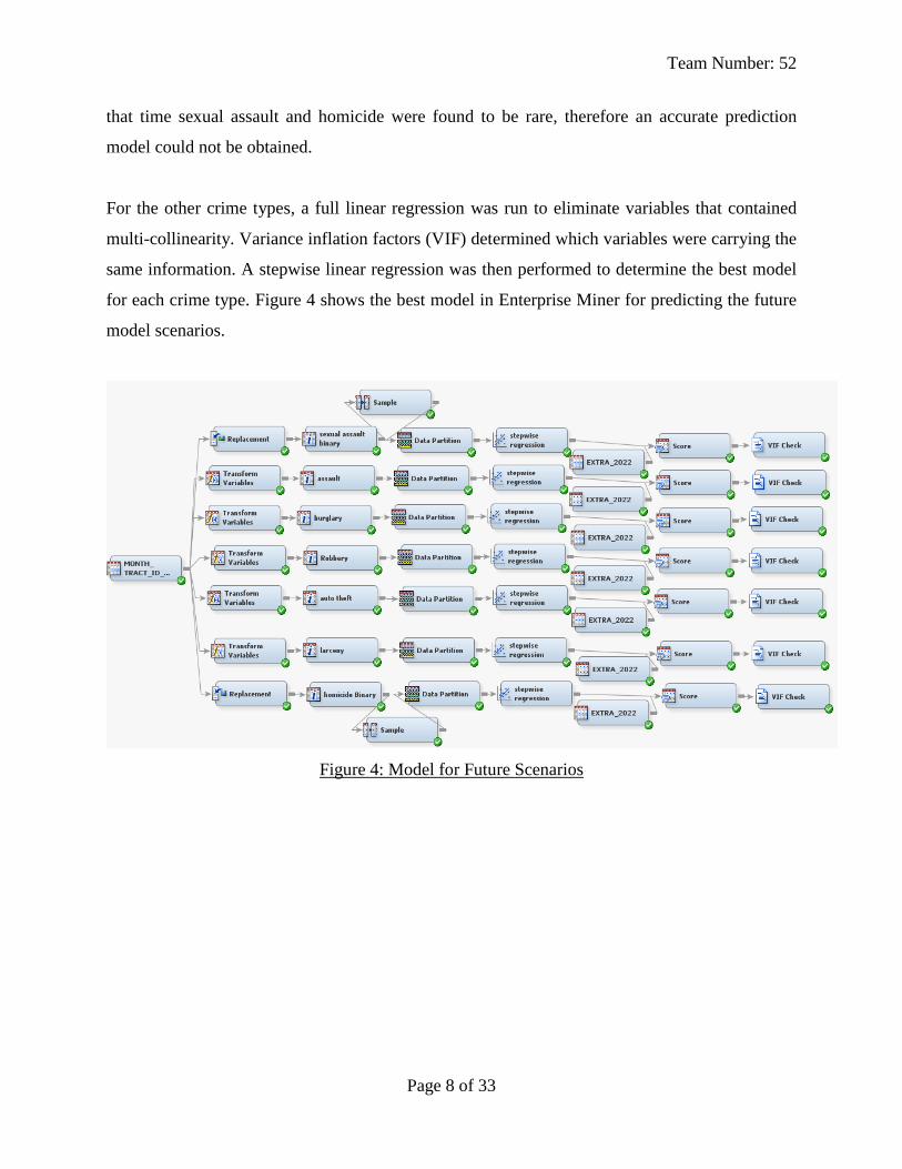
that time sexual assault and homicide were found to be rare, therefore an accurate prediction

model could not be obtained.

For the other crime types, a full linear regression was run to eliminate variables that contained

multi-collinearity. Variance inflation factors (VIF) determined which variables were carrying the

same information. A stepwise linear regression was then performed to determine the best model

for each crime type. Figure 4 shows the best model in Enterprise Miner for predicting the future

model scenarios.

Figure 4: Model for Future Scenarios

Team Number: 52

Page 9 of 33

5 EVALUATION

Stage five addresses the results from the models that have been

run to answer the questions as stated in our Problem Definition

in stage one.

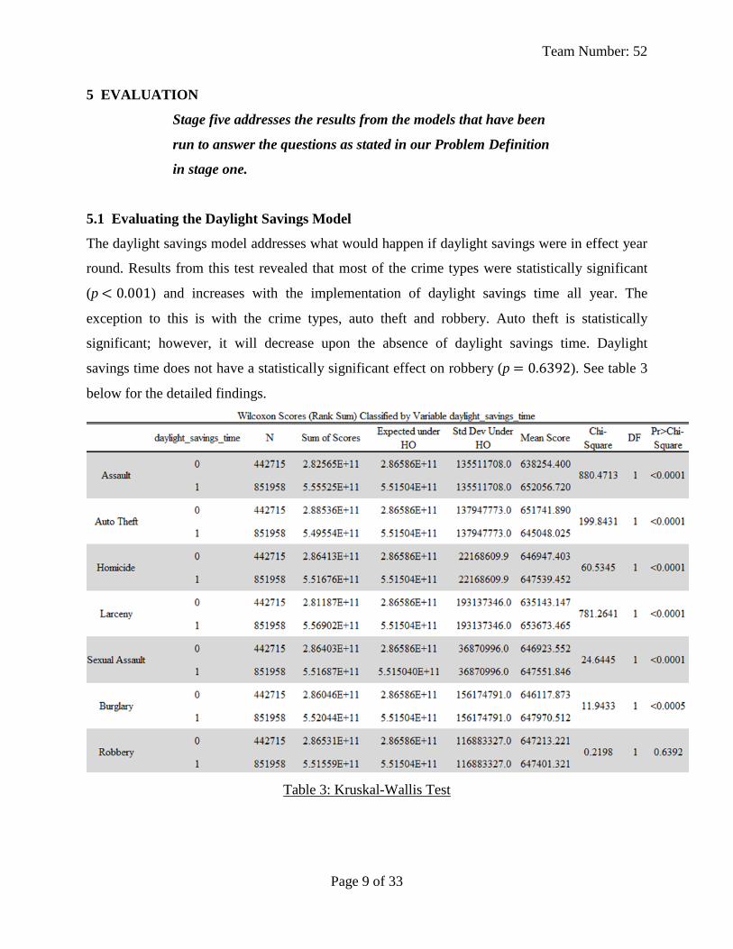
5.1 Evaluating the Daylight Savings Model

The daylight savings model addresses what would happen if daylight savings were in effect year

round. Results from this test revealed that most of the crime types were statistically significant

(p ) and increases with the implementation of daylight savings time all year. The

exception to this is with the crime types, auto theft and robbery. Auto theft is statistically

significant; however, it will decrease upon the absence of daylight savings time. Daylight

savings time does not have a statistically significant effect on robbery (p ). See table 3

below for the detailed findings.

Table 3: Kruskal-Wallis Test

Team Number: 52

Page 10 of 33

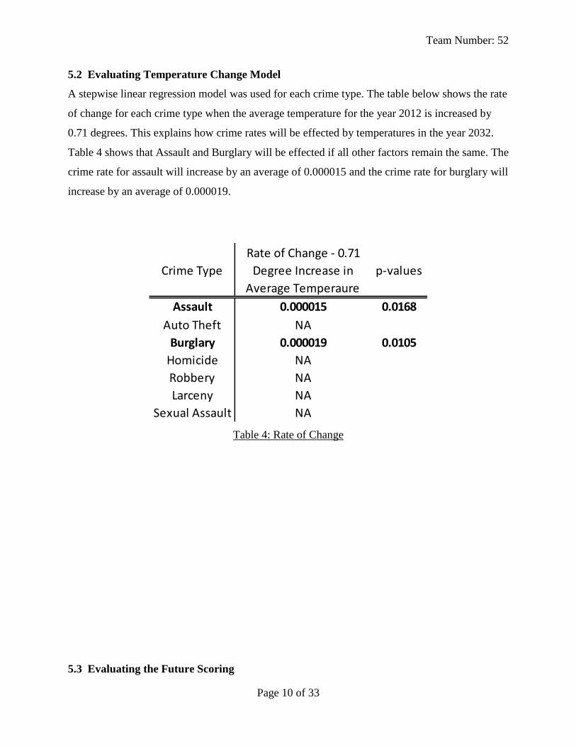
5.2 Evaluating Temperature Change Model

A stepwise linear regression model was used for each crime type. The table below shows the rate

of change for each crime type when the average temperature for the year 2012 is increased by

0.71 degrees. This explains how crime rates will be effected by temperatures in the year 2032.

Table 4 shows that Assault and Burglary will be effected if all other factors remain the same. The

crime rate for assault will increase by an average of 0.000015 and the crime rate for burglary will

increase by an average of 0.000019.

Table 4: Rate of Change

5.3 Evaluating the Future Scoring

Crime Type

Rate of Change - 0.71

Degree Increase in

Average Temperaure

p-values

Assault 0.000015 0.0168

Auto Theft NA

Burglary 0.000019 0.0105

Homicide NA

Robbery NA

Larceny NA

Sexual Assault NA

Team Number: 52

Page 11 of 33

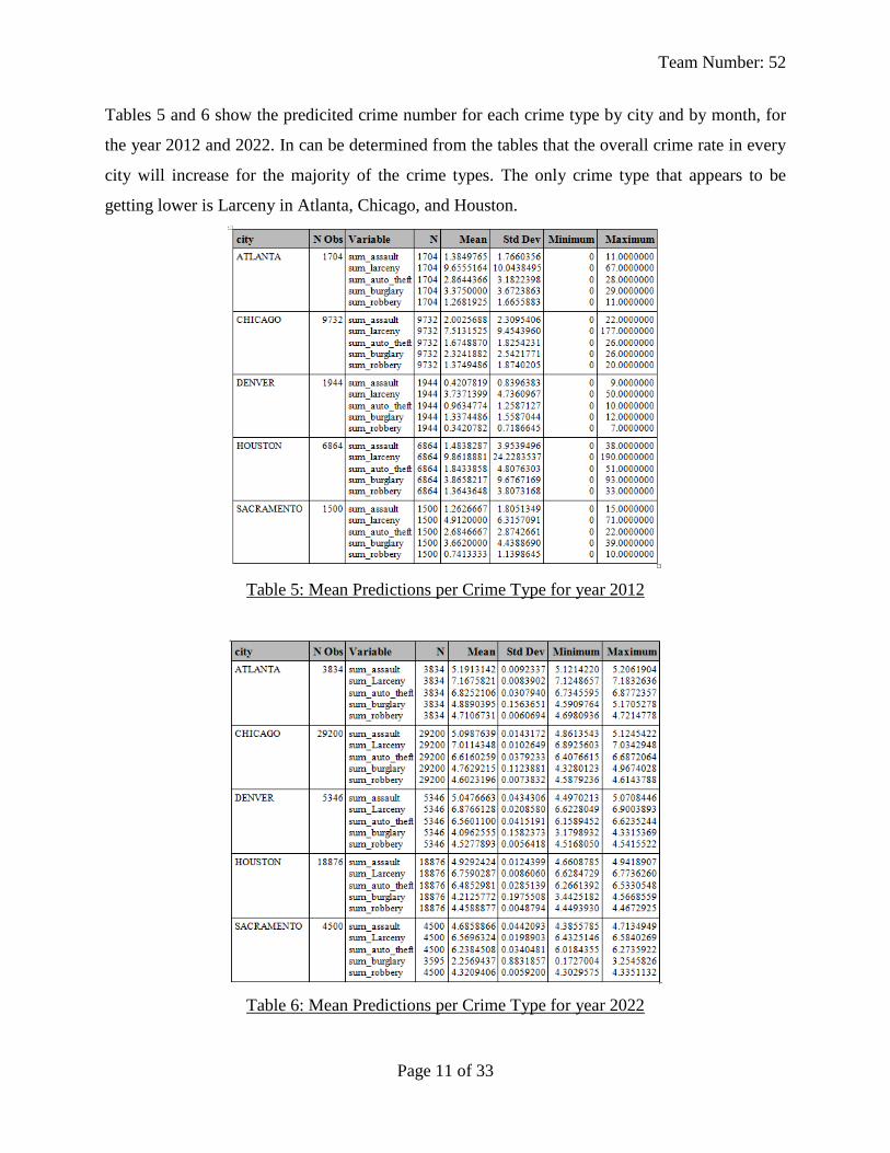
Tables 5 and 6 show the predicited crime number for each crime type by city and by month, for

the year 2012 and 2022. In can be determined from the tables that the overall crime rate in every

city will increase for the majority of the crime types. The only crime type that appears to be

getting lower is Larceny in Atlanta, Chicago, and Houston.

Table 5: Mean Predictions per Crime Type for year 2012

Table 6: Mean Predictions per Crime Type for year 2022

Team Number: 52

Page 12 of 33

6 CONCLUSIONS

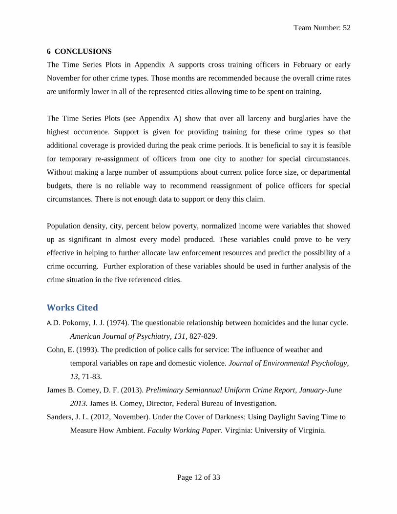
The Time Series Plots in Appendix A supports cross training officers in February or early

November for other crime types. Those months are recommended because the overall crime rates

are uniformly lower in all of the represented cities allowing time to be spent on training.

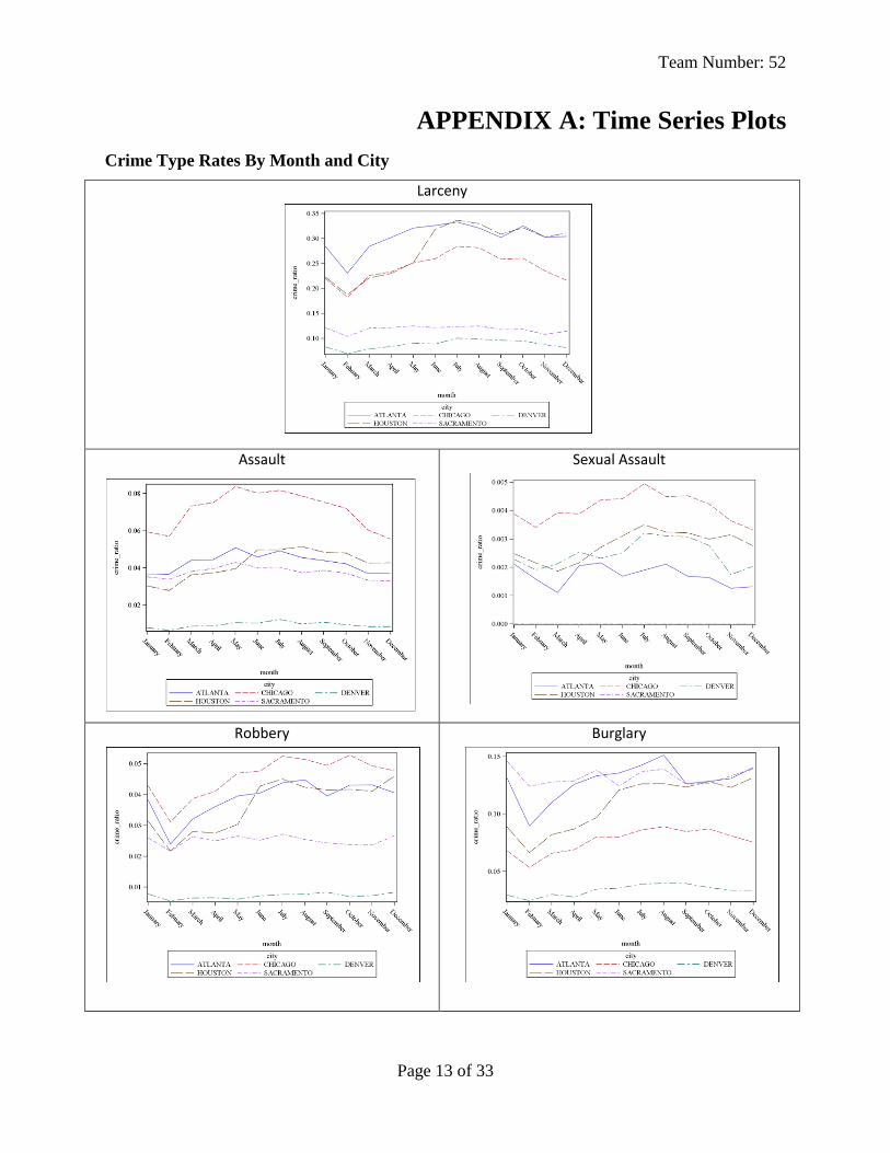
The Time Series Plots (see Appendix A) show that over all larceny and burglaries have the

highest occurrence. Support is given for providing training for these crime types so that

additional coverage is provided during the peak crime periods. It is beneficial to say it is feasible

for temporary re-assignment of officers from one city to another for special circumstances.

Without making a large number of assumptions about current police force size, or departmental

budgets, there is no reliable way to recommend reassignment of police officers for special

circumstances. There is not enough data to support or deny this claim.

Population density, city, percent below poverty, normalized income were variables that showed

up as significant in almost every model produced. These variables could prove to be very

effective in helping to further allocate law enforcement resources and predict the possibility of a

crime occurring. Further exploration of these variables should be used in further analysis of the

crime situation in the five referenced cities.

Works Cited

A.D. Pokorny, J. J. (1974). The questionable relationship between homicides and the lunar cycle.

American Journal of Psychiatry, 131, 827-829.

Cohn, E. (1993). The prediction of police calls for service: The influence of weather and

temporal variables on rape and domestic violence. Journal of Environmental Psychology,

13, 71-83.

James B. Comey, D. F. (2013). Preliminary Semiannual Uniform Crime Report, January-June

2013. James B. Comey, Director, Federal Bureau of Investigation.

Sanders, J. L. (2012, November). Under the Cover of Darkness: Using Daylight Saving Time to

Measure How Ambient. Faculty Working Paper. Virginia: University of Virginia.

Team Number: 52

Page 13 of 33

APPENDIX A: Time Series Plots

Crime Type Rates By Month and City

Larceny

Assault

Sexual Assault

Robbery

Burglary

Team Number: 52

Page 14 of 33

Homicide

Auto_Theft

Team Number: 52

Page 15 of 33

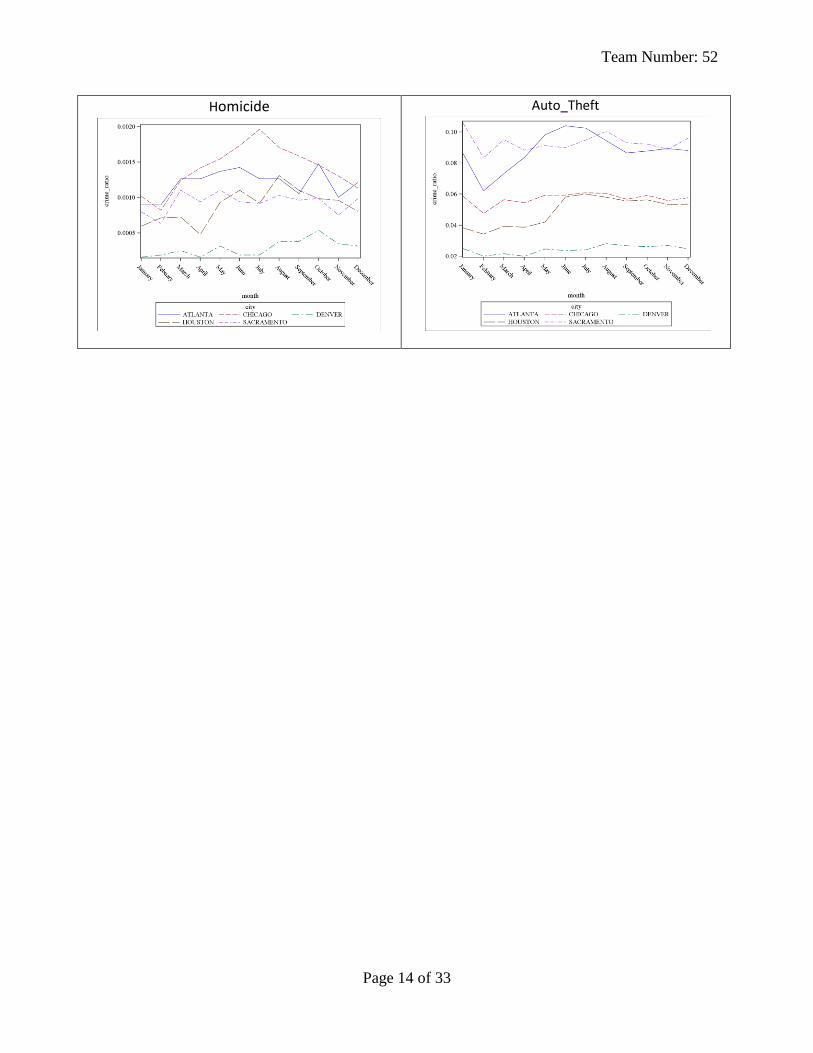
APPENDIX B: SAS Code Used

*The version of SAS used was SAS Base 9.3 and Enterprise Minor 7.1 Version

9.03.01;

*Please change the folder directory for the DATMIN library within the ‘ ’

below to the folder directory that includes the datasets specified in Step 0

in the file “SAS and Enterprise Miner Instructions”; LIBNAME DATMIN '' ;

***************************************************************************** ***************************************************************************** Data Set: Crime Data Goal: Create a binary response variable to indicate that a crime occurred.

This response variable will be used to compare crime occurred to no crime

occurred. We also created a numeric response to keep track of the total

number of crimes committed for future analysis. Next, crime type (Assault,

Burglary, etc.) is made into a variable. Lastly, the crime data set only

gives us the days a crime occurred. For example, if no crime were committed/

reported on January 2nd then no observation would be recorded for that day.

Some of the other data sets we were given have observations for every day of

the year. Unfortunately, if we were to merge the crime data set with these

data sets it would create a lot of missing entries. To overcome this we

modified the original crime data set by adding in the days of the year in which no crime occurred and filled in the missing information

appropriately. Objectives: 1. Create a binary and numeric response for days where a crime occurred. 2. Turn each crime type into its own variable within the crime dataset. 3. Create a data set that contains the completed records (Crime Type, City,

Day, etc.) for every day where no crimes occurred. 4. Merge the NO_CRIME data set with the CRIME_2 data set for a completed

data set that contains records for every day of the year. Output: At the end of this portion of code no output will be seen, but a new

data set CRIME_NEW will be created that has resolved the issue with the crime data set. We will begin merging everything

from here on out with the CRIME_NEW data set. CRIME_2 info: *after proc sort - variables = 12 and observations = 2205564 *after objective 1 - variables = 14 and observations =

1738711 CRIME_TRANS info: *variables = 10 and observations = 1298550 CRIMES info: *variables = 20 and observations = 1298550 NO_CRIME info: *variables = 3 and observations = 4283472 CRIME_NEW info: *variables = 27 and observations = 4283472 Comments from the Log: * None to report. ***************************************************************************** *****************************************************************************

Team Number: 52

Page 16 of 33

*sorts the data by tract_id and then date; PROC SORT DATA= DATMIN.CRIME_V2 OUT=CRIME_2; BY TRACT_ID DATE CRIME_TYPE; RUN; /* Objective 1 - Note that if Binary Response = 1 then a crime was committed,

all observations with a missing tract_id have been deleted, and "If LAST.DATE" is used to remove all duplicated

responses. Also, a numeric response was created to keep tract of the total number of crimes committed each day by

tract_id.*/ *CREATE NUMERIC RESPONSE, DELETE MISSING TRACT_IDS, REMOVE DUPLICATE OBSERVATIONS (BASED OF TRACT_ID AND DATE); DATA CRIME_2; SET CRIME_2; BY TRACT_ID DATE CRIME_TYPE; IF TRACT_ID = . THEN DELETE; BINARY_RESPONSE=1; IF AREA_RATIO=0 THEN DELETE; IF FIRST.CRIME_TYPE THEN CRIME= 1; ELSE CRIME+1; IF LAST.CRIME_TYPE; RUN; /*Objective 2 - Create a dataset CRIME_TRANS that lists crime types as a

variable, and then merges that dataset with the CRIMES dataset.*/ proc transpose data=crime_2 OUT = CRIME_TRANS let; by tract_id date; id crime_type; var CRIME; run; DATA CRIMES (DROP = _NAME_ CRIME); MERGE CRIME_2 CRIME_TRANS; BY TRACT_ID DATE; IF LAST.TRACT_ID OR LAST.DATE; RUN; /*Objective 3 – The NO_CRIME data set was created to keep a record of days in

each city where no crime occurred. The code below takes the crime data set and fills in any missing dates

(meaning a crime did not occur) between Jan. 1st – Dec. 31st with a “no crime” record and stores it in the NO_CRIME

data set. */ *CREATE BINARY NO CRIME DATA; DATA NO_CRIME; SET CRIME_2 (KEEP = CITY TRACT_ID); BY TRACT_ID; IF LAST.TRACT_ID; IF (CITY = 'SACRAMENTO' OR CITY= 'CHICAGO') THEN DO; DO DATE = '01JAN2005'D TO '31DEC2012'D; OUTPUT; END; END; ELSE IF (CITY = 'DENVER' OR CITY = 'HOUSTON') THEN DO; DO DATE = '01JAN2008'D TO '31DEC2012'D; OUTPUT;

Team Number: 52

Page 17 of 33

END; END; ELSE IF CITY = 'ATLANTA' THEN DO; DO DATE = '01JAN2009'D TO '31DEC2012'D; OUTPUT; END; END; FORMAT DATE DATE9.; RUN; /*Objective 4 – Takes both data sets (NO_CRIME and CRIMES) and merges them

together. This way each city has a completed record Jan.1st – Dec. 31st that contains every day of the year and whether

or not a crime committed. For days that did not have a crime and were added to the data set, the

variable hour was given a random integer 0-23 for the time of the crime using

the rand(UNIFORM) function. */ *MERGE NOCRIME AND CRIME DATA FILL IN VARIABLE VALUES FOR NOCRIME DATA; DATA CRIME_NEW (DROP=WDAY CRIME_TYPE); MERGE NO_CRIME CRIMES; BY TRACT_ID DATE; IF LARCENY= . THEN LARCENY=0; IF ASSAULT= . THEN ASSAULT = 0; IF SEXUAL_ASS= . THEN SEXUAL_ASS = 0; IF BURGLARY = . THEN BURGLARY = 0; IF AUTO_THEFT = . THEN AUTO_THEFT=0; IF ROBBERY= . THEN ROBBERY = 0; IF HOMICIDE = . THEN HOMICIDE = 0; IF LARCENY NE 0 THEN B_LARCENY=1; ELSE B_LARCENY = 0; IF ASSAULT NE 0 THEN B_ASSAULT=1; ELSE B_ASSAULT = 0; IF SEXUAL_ASS NE 0 THEN B_SEXUAL_ASS=1; ELSE B_SEXUAL_ASS = 0; IF BURGLARY NE 0 THEN B_BURGLARY =1; ELSE B_BURGLARY = 0; IF AUTO_THEFT NE 0 THEN B_AUTO_THEFT =1; ELSE B_AUTO_THEFT = 0; IF ROBBERY NE 0 THEN B_ROBBERY =1; ELSE B_ROBBERY = 0; IF HOMICIDE NE 0 THEN B_HOMICIDE =1; ELSE B_HOMICIDE = 0; NUMERIC_RESPONSE= lARCENY+ASSAULT+SEXUAL_ASS+BURGLARY+AUTO_THEFT+ROBBERY+HOMICIDE; IF ID = . THEN DO; YEAR = YEAR(DATE); MONTH=MONTH(DATE); DATE_NUM=DAY(DATE); WDAY=WEEKDAY(DATE); HOUR=FLOOR(RAND("UNIFORM")*24); BINARY_RESPONSE = 0; NUMERIC_RESPONSE= 0; CRIMEAREA='ALL'; END; IF WDAY = 1 THEN DAY= 'Sun'; ELSE IF WDAY = 2 THEN DAY = 'Mo'; ELSE IF WDAY = 3 THEN DAY = 'Tue'; ELSE IF WDAY = 4 THEN DAY = 'We'; ELSE IF WDAY = 5 THEN DAY = 'Thu'; ELSE IF WDAY = 6 THEN DAY = 'Fri'; ELSE IF WDAY = 7 THEN DAY = 'Sat'; RUN; ***************************************************************************** ***************************************************************************** Data Set: Unemployment Goal: The unemployment data set is fine as is. It just needs to be merged

together with the CRIME_NEW dataset. Objectives:

Team Number: 52

Page 18 of 33

1. Merge the unemployment data set with the CRIME_NEW data set. Output: At the end of this portion of code no output will be seen, but a new

data set CRIME_MERGE_UNEMPLOY will be created. UNEMPLOYMENT info: *variables = 5 and observations = 448704 CRIME_MERGE_UNEMPLOY info: * variables = 28 and observations = 4283472 Comments from the Log: *Note: Input data set (Unemployment) is already sorted, it has been

copied to the output data set. *****************************************************************************

***************************************************************************** *Objective 1- Sorts the data by TRACT_ID, YEAR, and then MONTH and merges it

with CRIME_NEW; PROC SORT DATA = datmin.unemployment out = unemployment; BY TRACT_ID YEAR MONTH; run; DATA CRIME_MERGE_UNEMPLOY (DROP=CITYNAME); MERGE CRIME_NEW UNEMPLOYMENT; BY TRACT_ID YEAR MONTH; IF DATE = . THEN DELETE;*Any unemployment data that has dates that do not

match with data CRIME_NEW gets deleted; RUN; ***************************************************************************** ***************************************************************************** Data Set: Socioeconomic Goal: The socioeconomic data set is fine as is. It just needs to be merged

together with the CRIME_MERGE_UNEMPLOY dataset. Objectives: 1. Merge the socioeconomic data set with the CRIME_MERGE_UNEMPLOY data set. Output: At the end of this portion of code no output will be seen, but a new

data set CRIME_MERGE_SOCIO will be created. SOCIOECON info: * variables = 6 and observations = 37392 CRIME_MERGE_SOCIO info: * variables = 31 and observations 4283472 Comments from the Log: *None to report *****************************************************************************

***************************************************************************** *Objective 1 - Sorts the Socioeconomic Data by tract_id and year and then

merges it with the CRIME_MERGE_UNEMPLOY dataset;

PROC SORT DATA = DATMIN.SOCIOECONOMIC out=SOCIOECON; BY TRACT_ID YEAR; RUN; DATA CRIME_MERGE_SOCIO; MERGE CRIME_MERGE_UNEMPLOY SOCIOECON; BY TRACT_ID YEAR; IF DATE = . THEN DELETE;*Any socioeconomic data that has dates that do not

match with data CRIME_NEW gets deleted; RUN; *****************************************************************************

Team Number: 52

Page 19 of 33

***************************************************************************** Data Set: Weather Goal: To use the weather data as is in addition to using the weather

information to calculate the heating and cooling information. This way the Heating_Cooling_Days does not have to be

merged into the larger dataset. Objectives: 1. Calculates the missing values in the Sacramento data. 2. Convert all the degrees into Fahrenheit and then calculate if the day

was a heating/cooling day and by how much. 3. Sorts the datasets by a common variable(s) and merges them together. Output: At the end of this portion of code no output will be seen, but a new

data set CRIME_MERGE_WEATHER will be created. WEATHER info: * variables = 14 and observations = 14610 CRIME_MERGE_SOCIO info: * variables = 31 and observations 4283472 CRIME_MERGE_WEATHER info: * variables = 41 and observations = 4283472 Comments from the Log: *After running the data weather set the following note was issued in the log. NOTE: Missing values were generated as a result of performing an

operation on missing values. Each place is given by: (Number of times) at (Line):(Column). 1 at 158:33 1 at 159:31 1 at 160:30 1 at 163:25 ***************************************************************************** *****************************************************************************

/* Objective 1 & 2 - Calculates the missing values in the Sacramento data.*/; DATA WEATHER; SET datmin.WEATHER; FORMAT DATE DATE9.; DROP DAY; TEMP_HIGH_F= (TEMPERATURE_HIGH*9)/5 +32; TEMP_LOW_F= (TEMPERATURE_LOW*9)/5 +32; /* 05/14/2012 sacramento has missing high/low temp so using 05/13 and 05/15

to fill in missing value */ if TEMP_HIGH_F=. then TEMP_HIGH_F=(75.02+80.96)/2; if TEMP_LOW_F=. then TEMP_LOW_F=(53.06+57.02)/2; /* 12/17/2006 sacramento has missing pressure so using 12/16 and 12/18 values

to fill in missing */ if pressure=. then pressure=(1010.2+1023.9)/2; AVERAGE_TEMP= (TEMP_HIGH_F + TEMP_LOW_F)/2; IF AVERAGE_TEMP < 65 THEN DO; DEGREE_DAY='HEATING'; TOTAL_DEGREE_DAY = 65-AVERAGE_TEMP; END; IF AVERAGE_TEMP > 65 THEN DO DEGREE_DAY = 'COOLING'; TOTAL_DEGREE_DAY = AVERAGE_TEMP -65; END; RUN; /* Objective 3 - Sorts the datasets by a common variable(s) and merges them

together.*/; *SORT BY CITY DATE SO IT CAN BE MERGED;

Team Number: 52

Page 20 of 33

PROC SORT DATA = WEATHER; BY CITY DATE; RUN;

PROC SORT DATA = CRIME_MERGE_SOCIO; BY CITY DATE; RUN;

*MERGE IN WEATHER; DATA CRIME_MERGE_WEATHER; MERGE CRIME_MERGE_SOCIO WEATHER; BY CITY DATE; IF CRIMEAREA = ' ' THEN DELETE; RUN; ***************************************************************************** ***************************************************************************** Data Set: Calendar Days Goal: To merge the CALENDAR_DAYS data into the combined data sets. This is

competed through the objectives below. Objectives: 1. Formatting the Calendar_days dataset to prepare it for the merger. 2. Sorting the CALDAYS dataset and the CRIME_MERGE_POP dataset and then

merging. Output: At the end of this portion of code the new combined data set

(CRIME_MERGE_CAL) has been created. CALDAYS info: *variables = 7 and observations = 7312 CRIME_MERGE_WEATHER info: *variables = 41 and observations = 4283472 CRIME_MERGE_CAL *variables = 47 and observations = 4283472 Log Comments: *None to report *****************************************************************************

***************************************************************************** *Objective 1 - All the dates in CALENDAR_DAYS is being reformatted to match

the other datasets (DDMonYYYY ex. 01Jan2008) and instead of blanks for non-holiday info the blanks

are being replaced with "NA" so that Enterprise Miner does not mistake these blanks as missing values;

/* Objective 1 - SFormatting the Calendar_days dataset to prepare it for the

merger.*/; DATA CALDAYS; SET DATMIN.CALENDAR_DAYS; FORMAT DATE DATE9.; IF HOLIDAYNAME='' THEN HOLIDAYNAME="NA"; IF HOLIDAY_WEEK='' THEN HOLIDAY_WEEK="NA"; RUN; /* Objective 2 - Sorting the CALDAYS dataset and the CRIME_MERGE_POP dataset

and then merging./; PROC SORT DATA = CALDAYS; BY DATE; RUN; PROC SORT DATA = CRIME_MERGE_WEATHER;

Team Number: 52

Page 21 of 33

BY DATE; RUN;

*MERGING CALENDAR_DAYS; /*CALDAYS does not contain a TRACT_ID so if there are dates that don’t align

the two data sets then those from CRIME_MERGE_WEATHER that are not included in CALDAYS are deleted*/; DATA CRIME_MERGE_CAL; MERGE CRIME_MERGE_WEATHER CALDAYS; BY DATE; IF TRACT_ID = . THEN DELETE; RUN;

***************************************************************************** ***************************************************************************** Data Set: Solar Lunar Goal: To merge the SOLAR_LUNAR data into the combined data sets and calculate

the total time from noon until sunset. This is competed through the objectives below. Objectives: 1. Formatting the SOLAR_LUNAR dataset to prepare it for the merger and

calculating the total time from noon until sunset. This calculation does take into account daylight savings

time. 2. Sorting the SOLLUN dataset and the CRIME_MERGE_CAL dataset and then

merging. Output: At the end of this portion of code the new combined data set

(CRIME_MERGE_SOLLUN) has been created. SOLLUN info: *variables = 9 and observations = 14610 CRIME_MERGE_CAL info: *variables = 47 and observations = 4283472 CRIME_MERGE_SOLLUN *variables = 54 and observations = 4283472 Log Comments: *None to report ***************************************************************************** ****************************************************************************; *Objective 1 - All the dates in SOLAR_LUNAR is reformatted to match the other

datasets (DDMonYYYY ex. 01Jan2008). Also, the number of number of hours between noon and sundown is calculated.

This also takes into account when daylight savings is in effect.; *Merging Solar_Lunar; DATA SOLLUN (DROP=NOON); SET DATMIN.SOLAR_LUNAR; FORMAT DATE DATE9.; IF DAYLIGHT_SAVINGS_TIME=0 THEN NOON = 43200;*12 hours * 60 minutes * 60

seconds = 43200; ELSE NOON = 39600; *If daylight savings is in effect then noon is 11am and

calculated similarly to the above calculation; DAYLIGHT_HOURS_AFTER_NOON=STANDARD_SUNSET - NOON; format DAYLIGHT_HOURS_AFTER_NOON TIME8.; *to get city names to "match" for merge; if city = "Atlanta" then city = "ATLANTA"; if city = "Chicago" then city = "CHICAGO";

Team Number: 52

Page 22 of 33

if city = "Denver" then city = "DENVER"; if city = "Houston" then city = "HOUSTON"; if city = "Sacramento" then city = "SACRAMENTO"; RUN; /*Objective 2 - Sorting both data sets by city and then date and merges them

together.*/ PROC SORT DATA = SOLLUN; BY CITY DATE; RUN; PROC SORT DATA = CRIME_MERGE_CAL; BY CITY DATE; RUN; /*SOLAR_LUNAR does not conatin a CRIME_TYPE so if there are cities/dates that

don't mesh up between the two data sets then those from CRIME_MERGE_CAL that are not included in SOLLUN are deleted*/ DATA CRIME_MERGE_SOLLUN; MERGE CRIME_MERGE_CAL SOLLUN; BY CITY DATE; if tract_id = . then delete; RUN; ***************************************************************************** ***************************************************************************** Data Set: Storms Goal: To expand the observations (days) in which a storm occurred so that

each storm day is its own observation, and then merges this new dataset with the big dataset. Objectives: 1. To expand the duration of each storm day into its own observation. 2. Sorting the storm dataset and then merging. Output: At the end of this portion of code the new combined data set

(CRIME_MERGE_STORM) has been created. STORM info: *variables = 9 and observations = 1483 CRIME_MERGE_STORM *variables = 61 and observations = 4283472 Log Notes: *After running the data storms step we got this note: NOTE: Character values have been converted to numeric values at the

places given by: (Line):(Column). 265:19 265:38 266:17 266:34 *After running the data CRIME_MERGE_STORM we got this note: NOTE: MERGE statement has more than one data set with repeats of BY

values ***************************************************************************** ****************************************************************************; /*Objective 1 - The original storm dataset indicated the start day of each

storm and how many days the storm lasted. For example, start date: January 1st and Duration: 3 days. We

needed each day the storm occurred to be its own observation, so that we could see if there were higher crime

rates on days that a storm was occurring. By the end of objective 1 the storm data will have an

observation for everyday of the storm. Using the same example as

Team Number: 52

Page 23 of 33

above, now instead of saying start date: January

1st and Duration: 3 days an observation is shown for January 1st, January 2nd, and January 3rd. Note

that only days where a storm was reported are observed. For instance, if there was no storm on March 2nd,

then there will not be an observation that corresponds to March 2nd.*/

*Merging Storms; data storm (KEEP= CITY STORM_CLASS BEGIN_TIME END_TIME BINARY_STORM

START_DATE END_DATE DAYS DATE ); set datmin.storms_V2; BINARY_STORM=1; bmonth =substrn(begin_yearmonth,5,2); byear = substrn(begin_yearmonth,1,4); emonth =substrn(end_yearmonth,5,2); eyear = substrn(end_yearmonth,1,4); start_date =mdy(bmonth, begin_day, byear); end_date =mdy(emonth, end_day, eyear); days = 1+(end_date - start_date); do i = 0 to days-1; IF I= 0 THEN DATE=START_DATE; ELSE DATE = DATE+1; output; end; FORMAT END_DATE START_DATE DATE DATE9.; run; /*Objective 2 - Sort the storm data and then merge it with the

CRIME_MERGE_SOLLUN dataset. Note that there will be dates in the CRIME_MERGE_SOLLUN dataset where no crime

occurred. If that is the case then that cell is marked with "NA", so that when the final data set is

uploaded into Enterprise Miner, Enterprise Miner does not treat those cells as missing data.*/ proc sort data = storm; by CITY DATE; run; DATA CRIME_MERGE_STORM; MERGE CRIME_MERGE_SOLLUN STORM; BY CITY DATE; IF CRIMEAREA=' ' THEN DELETE; if storm_class = " " then do; storm_class = "NA"; begin_time = .; end_time = .; binary_storm = 0; start_date = date; end_date = date; days = 0; end; RUN; *****************************************************************************

*****************************************************************************

Data Set: Population

Team Number: 52

Page 24 of 33

Goal: To create population densities and subdivide the population into

smaller groups for future analysis.

Objectives:

1. This code is used more to prepare the data for future

analysis by cleaning of some of the original data values.

The following changes were made:

a. Make a copy of the Population dataset called

population

b. Breaks the ages data into smaller groups (e.g.

Miners, Adults, etc.)based off of their age ranges.

This was done because in Enterprise Miner we wanted

to explore the idea that certain variables

might cause a rise of crime in various age groups.

c. Reformats the tract_id so it has a length of 12.

This prevents SAS from putting these values into

scientific notation and preserve the uniqueness of

each tract_id. Also, it takes some of the vaguer

ages (such as under 1) and assigns these character

values to a numeric integer

2. Finds the summation of all the population totals by year,

tract_id, gender, and then age group.

3. Sorts the data and removes any duplicates. We no longer need

individual ages. Instead we are know only concerned with the

age groups (minors, young adults, etc.)

4. Sorts the data so we can transpose the years. This is need in

order to do the do loops for the extrapolation calculation.

5. Extrapolates the data using an exponential function to

generate data for all the years.*/

6. Sorts the data for proc transpose. The proc transpose command

was used so that each age group (minors, adults, etc.)

is its own variable rather than just listed in a single column.

7. Sorting both data sets by city and then date and merges them

together.

Output:

Log Notes:

*None to Report

*****************************************************************************

****************************************************************************;

*Temporary copy to use when working with population; DATA BIG_DATA; SET CRIME_MERGE_STORM; RUN;

/* Objective 1 - This code is used more to prepare the data for future

analysis by cleaning of some of the original data values. The following changes were made: a. Make a copy of the Population dataset

called population b. Breaks the ages data into smaller

groups (e.g. Miners, Adults, etc.)based off of their age ranges. This was done because in

Enterprise Miner we wanted to explore the idea that certain variables might cause a rise of crime in

various age groups.

Team Number: 52

Page 25 of 33

c. Reformats the tract_id so it has a

length of 12. This prevents SAS from putting these values into scientific notation and

preserve the uniqueness of each tract_id. Also, it takes some of the vaguer ages (such as under 1) and

assigns these character values to a numeric integer */ /* Objective 1a */

DATA POPULATION; SET DATMIN.POPULATION_V2; RUN; /* Objective 1b */ proc format; value agefmt 0-17= 'Minors' 18-24='Young Adults' 25-34='Adults' 35-44='Older Adults' 45-65='Middle Aged' 65-80='Seniors' 81-high='Super Seniors'; run; /* Objective 1c - Changes age group called "Under_1" to "0" years,

"100_to_104" to "100" years, "105_to_109" to "105" years, and "110_and_over" to "110" years. */ data population2 (drop=age_group); set population; if age_group='under_1' then age=0;else if Age_group = "100_to_104" then age = 100; else if Age_group = "105_to_109" then age = 105; else if Age_group = "110_and_over" then age = 110; else age = input(Age_group, best8.); AgeGroup=PUT(Age,AGEFMT.);*converts AgeGroup variable from character to

numeric; format Tract_ID best12.;*converting Tract_ID variable to numeric

variable of length 12 rather than using "best10." format/informat; run; /* Objective 2 - Finds the summation of all the population totals by year,

tract_id, gender, and then age group. */ proc sql; create table pop3 as select *, sum(population) as group_Pop from population2 Group by Year, tract_id, GENDER, AGEGROUP; quit; /*Objective 3 - Sorts the data and removes any duplicates. We no longer need

individual ages. Instead we are know only concerned with the age groups (minors, young adults, etc.)*/

PROC SORT DATA =POP3 nodupkey OUT=POP4; BY YEAR TRACT_ID GENDER AGEGROUP; RUN; /*Objective 4 - Sorts the data so we can transpose the years. This is need in

order to do the do loops for the extrapolation calculation.*/

PROC SORT DATA=POP4 OUT=SORTED;

Team Number: 52

Page 26 of 33

BY TRACT_ID GENDER AGEGROUP; RUN; PROC TRANSPOSE DATA = SORTED OUT=POP_TRANS LET; ID YEAR; BY TRACT_ID GENDER AGEGROUP; VAR GROUP_POP; RUN; /*Objective 5 - Extrapolates the data using an exponential function to

generate data for all the years.*/ DATA POP6 (DROP=_2000 _2010 RATE _NAME_); SET POP_TRANS; IF _2000 AND _2010 NE 0 THEN DO; DO YEAR=2000 TO 2012; RATE=(1/10)*LOG(_2010/_2000); PREDICT_POP=_2000*EXP(RATE*(YEAR-2000)); OUTPUT; END; END; RUN; /*Objective 6 - Sorts the data for proc transpose. The proc transpose command

was used so that each age group (minors, adults, etc.) is its own variable rather than just listed in a

single column. */ PROC SORT DATA = POP6; BY TRACT_ID YEAR; RUN; PROC TRANSPOSE DATA=POP6 OUT=POP7 (DROP=_NAME_); ID AGEGROUP GENDER; BY TRACT_ID YEAR; RUN; /*Objective 7 - Sorting both data sets by city and then date and merges them

together.*/

PROC SORT DATA=POPULATION2 NODUPKEY OUT=POP2_SORTED; BY TRACT_ID YEAR; RUN; PROC SORT DATA = POP7; BY TRACT_ID; RUN; DATA MERGED (DROP=I); MERGE POP2_SORTED (KEEP=CITY TRACT_ID TRACT_AREA) POP7; BY TRACT_ID; ARRAY TEST_MISS(*) _NUMERIC_; DO I=1 TO DIM(TEST_MISS); IF TEST_MISS(I) = . THEN TEST_MISS(I)=0; END; fem_total=adultsfemale + middle_agedfemale + minorsfemale +

older_adultsfemale + seniorsfemale + super_seniorsfemale +

young_adultsfemale; male_total=adultsmale + middle_agedmale + minorsmale + older_adultsmale

+ seniorsmale + super_seniorsmale + young_adultsmale; Total_pop = fem_total+male_total; adults_total= adultsfemale+adultsmale; middle_aged_total= middle_agedfemale+ middle_agedmale; minors_total= minorsfemale+minorsmale; older_adults_TOTAL= older_adultsFEMALE+older_adultsMALE;

Team Number: 52

Page 27 of 33

SENIORS_TOTAL=seniorsfemale+seniorsmale; super_seniors_TOTAL= super_seniorsfemale+super_seniorsmale; young_adults_TOTAL= young_adultsfemale+young_adultsmale; RUN; /*Created pop densities stuff 1st array for diff age groups 2nd array where

he is going to place density info then uses doloop to set popdensities for

each group*/

data popdens; set merged; array population {24} adultsfemale middle_agedfemale minorsfemale

older_adultsfemale seniorsfemale super_seniorsfemale young_adultsfemale adultsmale middle_agedmale minorsmale older_adultsmale seniorsmale

super_seniorsmale young_adultsmale fem_total male_total Total_pop

adults_total middle_aged_total minors_total older_adults_TOTAL SENIORS_TOTAL super_seniors_TOTAL

young_adults_TOTAL; array popdense{24} popdense_adultsfemale popdense_middle_agedfemale

popdense_minorsfemale popdense_older_adultsfemale popdense_seniorsfemale

popdense_super_seniorsfemale popdense_young_adultsfemale popdense_adultsmale popdense_middle_agedmale popdense_minorsmale

popdense_older_adultsmale popdense_seniorsmale popdense_super_seniorsmale

popdense_young_adultsmale popdense_fem_total popdense_male_total popdense_Total_pop popdense_adults_total

popdense_middle_aged_total popdense_minors_total popdense_older_adults_TOTAL popdense_SENIORS_TOTAL

popdense_super_seniors_TOTAL popdense_young_adults_TOTAL; do i = 1 to 24; popdense{i}=population{i}/tract_area; population{i}=round(population{i},1); end; run; /*sort to merge*/ proc sort data=big_data; by tract_id year; run; Data Big_data2; merge big_data popdens; by tract_id year; if date=. then delete; run; *Create Crime Ratio variable; data big; set big_data2; STORM_DAYS= (DATE-

START_DATE)+1;

IF BINARY_STORM= 0 THEN

STORM_DAYS=0;

If Holiday_Week = 'NA' THEN

B_HOLIDAY_WEEK=0;

Team Number: 52

Page 28 of 33

ELSE

B_HOLIDAY_WEEK=1;

If HolidayNAME = 'NA' THEN

B_HOLIDAY_NAME=0;

ELSE

B_HOLIDAY_NAME=1;

IF DAYLIGHT_SAVINGS_TIME=0 THEN

SUNRISE_MIN=STANDARD_SUNRISE/60;

ELSE IF DAYLIGHT_SAVINGS_TIME=1

THEN SUNRISE_MIN=(STANDARD_SUNRISE/60)+60;

IF DAYLIGHT_SAVINGS_TIME=0 THEN

SUNSET_MIN=STANDARD_SUNSET/60;

ELSE IF DAYLIGHT_SAVINGS_TIME=1 THEN

SUNSET_MIN=(STANDARD_SUNSET/60)+60; run; *******************Crime Data Set******************; *Create Crime Ratio variable; data big_cr; set BIG; IF Total_pop NE 0 THEN

CRIME_RATIO=NUMERIC_RESPONSE/Total_pop*100;

ELSE CRIME_RATIO=0; IF Total_pop NE 0 THEN

ASSAULT_CRIME_RATIO=ASSAULT/Total_pop*100;

ELSE ASSAULT_CRIME_RATIO=0; IF Total_pop NE 0 THEN

AUTO_THEFT_CRIME_RATIO=AUTO_THEFT/Total_pop*100;

ELSE AUTO_THEFT_CRIME_RATIO=0; IF Total_pop NE 0 THEN

BURGLARY_CRIME_RATIO=BURGLARY/Total_pop*100;

ELSE BURGLARY_CRIME_RATIO=0;

Team Number: 52

Page 29 of 33

IF Total_pop NE 0 THEN

HOMICIDE_CRIME_RATIO=HOMICIDE/Total_pop*100;

ELSE HOMICIDE_CRIME_RATIO=0; IF Total_pop NE 0 THEN

LARCENY_CRIME_RATIO=LARCENY/Total_pop*100;

ELSE LARCENY_CRIME_RATIO=0; IF Total_pop NE 0 THEN

ROBBERY_CRIME_RATIO=ROBBERY/Total_pop*100;

ELSE ROBBERY_CRIME_RATIO=0; IF Total_pop NE 0 THEN

SEXUAL_ASS_CRIME_RATIO=SEXUAL_ASS/Total_pop*100;

ELSE SEXUAL_ASS_CRIME_RATIO=0; run;

*Below creates a datetime formatted variable accounting for the length of

time between crime to storm start time and storm end time; data TIMES ; set big_cr; crime_time=catx(':',put(hour,z2.),'00'); /*convert hour to time of crime by adding 0's for mins/secs and

converting to time8 format */ crime_time=catx(':',crime_time,'00'); crime_time=input(crime_time,time8.);/* create crime time and format it to

datetime */ crime_timedate=dhms(date,0,0,crime_time); format crime_timedate datetime13.; if begin_time<1000 then do; begin_time2=put(begin_time,z3.);/* convert to char */ begin_hour=substr(begin_time2,1,1);/* get hour*/ begin_minutes=substr(begin_time2,2,2);/*get mins */ t=catx('',begin_hour,begin_minutes);/*mins and secs together */ t1=input(t,time8.); /* convert to time */ storm_start=dhms(date,0,0,t1); /* convert to datetime */ format storm_start datetime13.; end; if begin_time>=1000 then do; begin_time3=put(begin_time,z4.); begin_hour=substr(begin_time3,1,2);/* get hour*/ begin_minutes=substr(begin_time3,3,2);/*get mins */ t=catx('',begin_hour,begin_minutes); t1=input(t,time8.);

Team Number: 52

Page 30 of 33

storm_start=dhms(date,0,0,t1); format storm_start datetime13.; end; if end_time<1000 then do; end_time2=put(end_time,z3.); end_hour=substr(end_time2,1,1); end_minutes=substr(end_time2,2,2); t=catx('',end_hour,end_minutes); t1=input(t,time8.); storm_end=dhms(date,0,0,t1); format storm_end datetime13.; end; if end_time>=1000 then do; end_time3=put(end_time,z4.); end_hour=substr(end_time3,1,2); end_minutes=substr(end_time3,3,2); t=catx('',end_hour,end_minutes); t1=input(t,time8.); storm_end=dhms(date,0,0,t1); format storm_end datetime13.; end; if binary_storm = 1 then S_end= storm_end; retain s_end; run; data TIME_STORMS (drop=s_end end_time3 end_minutes end_hour end_time2 x); set TIMES; if binary_response= 1 then x=s_end; else x= .; if crime_timedate-x > 1209600 theN X =.; time_since_last_Storm= crime_timedate-x; IF TIME_SINCE_LAST_STORM=. AND BINARY_RESPONSE= 1 THEN

TIME_SINCE_LAST_STORM=1209601; IF TIME_SINCE_LAST_STORM < 0 AND TIME_SINCE_LAST_STORM NE . THEN

TIME_SINCE_LAST_STORM=0; IF BINARY_STORM=1 AND BINARY_RESPONSE= 1 THEN TIME_SINCE_LAST_STORM=0.1; run; data TIME_STORMS2; set TIME_STORMS (drop=t begin_time3 begin_hour begin_minutes begin_time2

t1); if binary_Storm=0 then storm_start=.; if binary_Storm=0 then storm_end=.; time_until_storm_ends=storm_end-crime_timedate; time_since_storm_started=crime_timedate-storm_start; IF time_until_storm_ends=0 THEN time_until_storm_ends=0.1; IF time_until_storm_ends =. THEN time_until_storm_ends=0; IF time_since_storm_started=0 THEN time_since_storm_started=0.1; IF time_since_storm_started=. THEN time_since_storm_started=0; run;

*Creates permanent datasets (Tali & Tali_Crimes); DATA DATMIN.TALI; SET TIME_STORMS2; RUN;

Team Number: 52

Page 31 of 33

data DATMIN.TALI_CRIMES; set TIME_STORMS2; if binary_response=1; run; *Create Data set with averages and sum by month or year; data DATMIN.TALI; set TIME_STORMS2 (drop=i); run;

proc sql; create table average_sum as select sum(school_day), tract_id, city, month(date) as month, year(date)

as year, mean(average_temp) as avg_average_temp, mean(cloud_cover) as

avg_Cloud_cover, mean(daylight_hours_after_noon) as avg_daylight_hours_after_noon,

mean(pressure) as avg_pressure, sum(assault) as sum_assault, sum(Auto_theft) as sum_auto_theft, sum(burglary) as sum_burglary,

sum(homicide) as sum_Homicide, sum(larceny) as sum_larceny, sum(Robbery) as sum_robbery, sum(sexual_ass) as sum_sexual_ass,

sum(Numeric_response) as Sum_crimes, mean(precipitation) as avg_precipitation, MEAN(SUNRISE_MIN) as sunrise, mean(SUNSET_MIN) as

sunset, sum(precipitation) as sum_precipitation, mean(temp_high_F) as

avg_temp_high_F, mean(temp_low_F) as avg_temp_low_F, sum(school_day) as sum_school_day,

sum(full_moon) as sum_Full_moon, sum(full_moon_group) as sum_full_moon_group, mean(standard_sunrise) as

avg_Standard_sunrise, mean(standard_sunset) as avg_Standard_sunset,sum(binary_storm) as

sum_binary_storm,mean(crime_ratio) as avg_crime_ratio,sum(minorsfemale) as

fem_Minors, sum(young_adultsfemale) as Fem_YoungAdults, sum(adultsfemale) as Fem_Adults, sum(older_adultsfemale) as older_Fem_Adults,

sum(middle_agedfemale) as fem_MiddleAged, sum(seniorsfemale) as Fem_Seniors, sum(super_seniorsfemale) as Fem_SuperSeniors,

sum(minorsmale) as Male_Minors, Sum(young_adultsmale) as Male_YoungAdults, sum(adultsmale) as Male_OlderYoungAdults,

sum(adultsmale) as Male_Adults, sum(middle_agedmale) as Male_MiddleAged, sum(seniorsmale) as

Male_Seniors, sum(super_seniorsmale) as Male_SuperSeniors, mean(unemplyment_rate) as avg_Unemployment_rate, mean(normalincome) as

Avg_NormalIncome, avg(dropoutrate) as avg_dropoutrate,sum(tract_area) as

city_tract_area , mean(pct_below_poverty) as avg_pct_below_poverty, sum(fem_total) as

Femal_total, sum(male_total) as c_male_total, sum(Total_pop) as city_pop,

sum(adults_total)as adult_total, sum(middle_aged_total) as total_middle_aged, sum(minors_total) as

total_minors, sum(older_adults_TOTAL) as total_older_adults,

sum(SENIORS_TOTAL) as total_seniors, sum(super_seniors_TOTAL) as total_super_seniors, sum(young_adults_TOTAL)

as total_young_adults from datmin.final_alls group by tract_id, year, month; quit; data average_sum2; set average_sum; BY TRACT_ID YEAR MONTH; if last.month;

Team Number: 52

Page 32 of 33

if avg_average_temp> 65 then Heating=0; else if avg_average_temp < 65 then Heating= 65-avg_average_temp; if avg_average_temp < 65 then cooling=0; else if avg_average_temp > 65 then cooling= avg_average_temp-65; format avg_daylight_hours_after_noon time8. avg_standard_sunrise time8.

avg_standard_sunset time8.; run;

data city_popdens; set AVERAGE_SUM2; array population {24} fem_Minors Fem_YoungAdults Fem_Adults older_Fem_Adults fem_MiddleAged Fem_Seniors

Fem_SuperSeniors Male_Minors Male_YoungAdults Male_OlderYoungAdults

Male_Adults Male_MiddleAged Male_Seniors Male_SuperSeniors Femal_total

c_male_total city_pop adult_total total_middle_aged total_minors

total_older_adults total_seniors total_super_seniors total_young_adults; array popdense{24} popdense_fem_Minors popdense_Fem_YoungAdults popdense_Fem_Adults popdense_older_Fem_Adults

popdense_fem_MiddleAged popdense_Fem_Seniors popdense_Fem_SuperSeniors

popdense_Male_Minors popdense_Male_YoungAdults popdense_Male_OlderYoungAdults

popdense_Male_Adults popdense_Male_MiddleAged popdense_Male_Seniors

popdense_Male_SuperSeniors popdense_Femal_total popdense_c_male_total

popdense_city_pop popdense_adult_total popdense_total_middle_aged

popdense_total_minors popdense_total_older_adults popdense_total_seniors popdense_total_super_seniors

popdense_total_young_adults; do i = 1 to 24; popdense{i}=population{i}/city_tract_area; end; run; *Creates permenent dataset (Month_TRACT_ID_crime); data datmin.Month_TRACT_ID_crime; set city_popdens; run;