Saraswati introductory microeconomics Material/Micro Economic... · involved in designing a project...
372
Strictly in accordance with the latest syllabus prescribed by CBSE, New Delhi and adopted by various boards, like—Haryana School Education Board, Bhiwani; Jharkhand Academic Council, Ranchi; and Bihar School Examination Board, Patna. Saraswati INTRODUCTORY MICROECONOMICS [For Class XI] By Dr. Deepashree Associate Professor in Economics Department of Commerce Shri Ram College of Commerce University of Delhi, Delhi New Saraswati House (India) Pvt. Ltd. New Delhi-110002 (INDIA)
Transcript of Saraswati introductory microeconomics Material/Micro Economic... · involved in designing a project...
Strictly in accordance with the latest syllabus prescribed by CBSE, New Delhi and adopted by various boards, like—Haryana School Education Board, Bhiwani; Jharkhand Academic Council, Ranchi; and
Bihar School Examination Board, Patna.
Saraswati
introductorymicroeconomics
[For Class xi]
By
Dr. DeepashreeAssociate Professor in Economics
Department of CommerceShri Ram College of Commerce
University of Delhi, Delhi
New Saraswati House (india) Pvt. Ltd.New Delhi-110002 (INDIA)
Second Floor, MGM Tower, 19 Ansari Road, Daryaganj, New Delhi-110002 (India) Phone : +91-11-43556600Fax : +91-11-43556688E-mail : [email protected] : www.saraswatihouse.comCIN : U22110DL2013PTC262320Import-Export Licence No. 0513086293
Branches:
• Ahmedabad (079) 22160722 • Bengaluru (080) 26619880, 26676396 • Bhopal +91-7554003654 • Chennai (044) 28416531 • Dehradun 09837452852• Guwahati (0361) 2457198 • Hyderabad (040) 42615566 • Jaipur (0141) 4006022 • Jalandhar (0181) 4642600, 4643600 • Kochi (0484) 4033369 • Kolkata (033) 40042314 • Lucknow (0522) 4062517 • Mumbai (022) 28737050, 28737090 • Nagpur +91-7066149006 • Patna (0612) 2275403 • Ranchi (0651) 2244654
New edition 2018
ISBN: 978-93-5272-518-2
Published by: New Saraswati House (India) Pvt. Ltd.19 Ansari Road, Daryaganj, New Delhi-110002 (India)
The moral rights of the author has been asserted.
©Reserved with the Publishers
All rights reserved under the Copyright Act. No part of this publication may be reproduced, transcribed, transmitted, stored in a retrieval system or translated into any language or computer, in any form or by any means, electronic, mechanical, magnetic, optical, chemical, manual, photocopy or otherwise without the prior permission of the copyright owner. Any person who does any unauthorised act in relation to this publication may be liable to criminal prosecution and civil claims for damages.
Printed at: Vikas Publishing House Pvt. Ltd., Sahibabad (Uttar Pradesh)
Product Code: NSS3IME110ECNAB17CBN
This book is meant for educational and learning purposes. The author(s) of the book has/have taken all reasonable care to ensure that the contents of the book do not violate any copyright or other intellectual property rights of any person in any manner whatsoever. In the event the author(s) has/have been unable to track any source and if any copyright has been inadvertently infringed, please notify the publisher in writing for any corrective action.

It gives me great pleasure in presenting the revised edition of ‘Saraswati Introductory Microeconomics’, according to the latest syllabus prescribed by CBSE.
Some unique features of this book are:• Clear and precise exposition of the subject.• A brief Chapter Scheme outlining the contents of the Chapter.• The analysis in each Chapter is developed in a step-by-step, systematic manner,
based on logical reasoning.• Points to Remember have been given at the end of every Chapter.• Chapterwise questions under the heading—Test Your Knowledge have been
given to enhance and cross-check the understanding of the subject. They are set on the pattern of the Board examination.
• Seven unsolved Practice Papers.• A large number of figures, examples and tables give complete knowledge of
various concepts.• A large number of solved numerical problems have also been given.• Many new concepts given in NCERT book have been given under the title
Annexure.• Completely covers the NCERT book and CBSE supplementary reading.• Value Based and Higher Order Thinking Questions (HoTS Questions) with
answers have been given at the end of each unit.• Answers to NCERT textual questions have been given at the end of each unit.• MCQs have been included in every chapter.The book is a product of thirty three years of my teaching experience and personal
interaction with the commerce and economics students at Shri Ram College of Commerce, University of Delhi, Delhi. Through them, I have learnt the needs and requirements of the senior secondary school students. I am of the opinion that such students must be made to imbibe fundamental knowledge in a simple and scientific way.
over the years, I have received many suggestions from teachers and students. I am thankful to them for their valuable inputs.
I am specially thankful to the Publisher, New Saraswati House (India) Pvt. Ltd., for giving me an opportunity to work for them.
Last but not the least, my heartfelt gratitude to Sushil, Sudeep and Saumya. Without their love and cooperation, I would have never been able to complete this book.
April 2018
Preface
(iii)

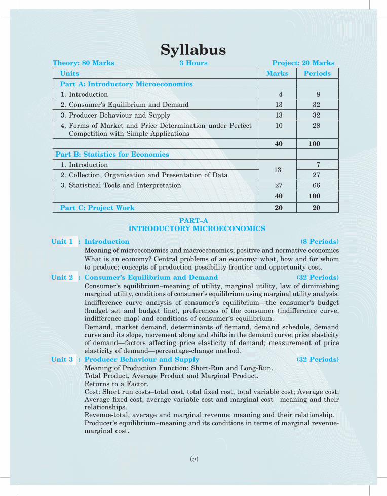
SyllabusTheory: 80 Marks 3 Hours Project: 20 Marks
Units Marks PeriodsPart A: Introductory Microeconomics
1. Introduction 4 8 2. Consumer’s Equilibrium and Demand 13 32 3. Producer Behaviour and Supply 13 32 4. Forms of Market and Price Determination under Perfect
Competition with Simple Applications 10 28
40 100Part B: Statistics for Economics 1. Introduction
13 7
2. Collection, organisation and Presentation of Data 27 3. Statistical Tools and Interpretation 27 66
40 100
Part C: Project Work 20 20
PART–A INTRODUCTORY MICROECONOMICS
Unit 1 : Introduction (8 Periods) Meaning of microeconomics and macroeconomics; positive and normative economics What is an economy? Central problems of an economy: what, how and for whom
to produce; concepts of production possibility frontier and opportunity cost. Unit 2 : Consumer’s Equilibrium and Demand (32 Periods) Consumer’s equilibrium–meaning of utility, marginal utility, law of diminishing
marginal utility, conditions of consumer’s equilibrium using marginal utility analysis. Indifference curve analysis of consumer’s equilibrium—the consumer’s budget
(budget set and budget line), preferences of the consumer (indifference curve, indifference map) and conditions of consumer’s equilibrium.
Demand, market demand, determinants of demand, demand schedule, demand curve and its slope, movement along and shifts in the demand curve; price elasticity of demand—factors affecting price elasticity of demand; measurement of price elasticity of demand—percentage-change method.
Unit 3 : Producer Behaviour and Supply (32 Periods) Meaning of Production Function: Short-Run and Long-Run. Total Product, Average Product and Marginal Product. Returns to a Factor. Cost: Short run costs–total cost, total fixed cost, total variable cost; Average cost;
Average fixed cost, average variable cost and marginal cost—meaning and their relationships.
Revenue-total, average and marginal revenue: meaning and their relationship. Producer’s equilibrium–meaning and its conditions in terms of marginal revenue-
marginal cost.
(v)
(vi)
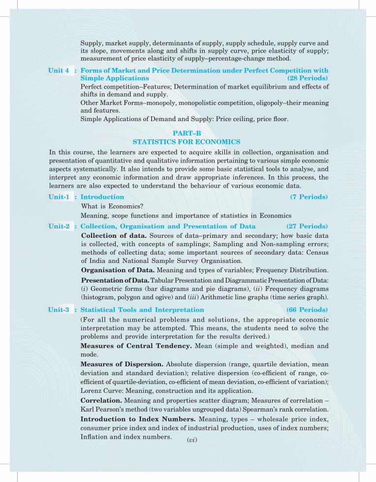
Supply, market supply, determinants of supply, supply schedule, supply curve and its slope, movements along and shifts in supply curve, price elasticity of supply; measurement of price elasticity of supply–percentage-change method.
Unit 4 : Forms of Market and Price Determination under Perfect Competition with Simple Applications (28 Periods)
Perfect competition–Features; Determination of market equilibrium and effects of shifts in demand and supply.
other Market Forms–monopoly, monopolistic competition, oligopoly–their meaning and features.
Simple Applications of Demand and Supply: Price ceiling, price floor.
PART–B STATISTICS FOR ECONOMICS In this course, the learners are expected to acquire skills in collection, organisation and
presentation of quantitative and qualitative information pertaining to various simple economic aspects systematically. It also intends to provide some basic statistical tools to analyse, and interpret any economic information and draw appropriate inferences. In this process, the learners are also expected to understand the behaviour of various economic data.
Unit-1 : Introduction (7 Periods) What is Economics? Meaning, scope functions and importance of statistics in Economics
Unit-2 : Collection, Organisation and Presentation of Data (27 Periods) Collection of data. Sources of data–primary and secondary; how basic data
is collected, with concepts of samplings; Sampling and Non-sampling errors; methods of collecting data; some important sources of secondary data: Census of India and National Sample Survey organisation.
Organisation of Data. Meaning and types of variables; Frequency Distribution.
Presentation of Data. Tabular Presentation and Diagrammatic Presentation of Data: (i) Geometric forms (bar diagrams and pie diagrams), (ii) Frequency diagrams (histogram, polygon and ogive) and (iii) Arithmetic line graphs (time series graph).
Unit-3 : Statistical Tools and Interpretation (66 Periods) (For all the numerical problems and solutions, the appropriate economic
interpretation may be attempted. This means, the students need to solve the problems and provide interpretation for the results derived.)
Measures of Central Tendency. Mean (simple and weighted), median and mode.
Measures of Dispersion. Absolute dispersion (range, quartile deviation, mean deviation and standard deviation); relative dispersion (co-efficient of range, co-efficient of quartile-deviation, co-efficient of mean deviation, co-efficient of variation); Lorenz Curve: Meaning, construction and its application.
Correlation. Meaning and properties scatter diagram; Measures of correlation – Karl Pearson’s method (two variables ungrouped data) Spearman’s rank correlation.
Introduction to Index Numbers. Meaning, types – wholesale price index, consumer price index and index of industrial production, uses of index numbers; Inflation and index numbers.

PART C:
DEVElOPINg PROjECTS IN ECONOMICS (20 Periods)
The students may be encouraged to develop projects, as per the suggested project guidelines. Case studies of a few organisations/outlets may also be encouraged. Under this the students will do only one comprehensive projects using concepts from both part A and part B.
Some of the examples of the projects are as follows (they are not mandatory but suggestive): (i) A report on demographic structure of your neighborhood. (ii) Changing consumer awareness amongst households. (iii) Dissemination of price information for growers and its impact on consumers. (iv) Study of a cooperative institution: milk cooperatives, marketing cooperatives, etc. (v) Case studies on public private partnership, outsourcing and outward Foreign Direct Investment. (vi) Global warming. (vii) Designing eco-friendly projects applicable in school such as paper and water recycle.
The idea behind introducing this unit is to enable the students to develop the ways and means by which a project can be developed using the skills learned in the course. This includes all the steps involved in designing a project starting from choosing a title, exploring the information relating to the title, collection of primary and secondary data, analysing the data, presentation of the project and using various statistical tools and their interpretation and conclusion.
(vii)
(viii)
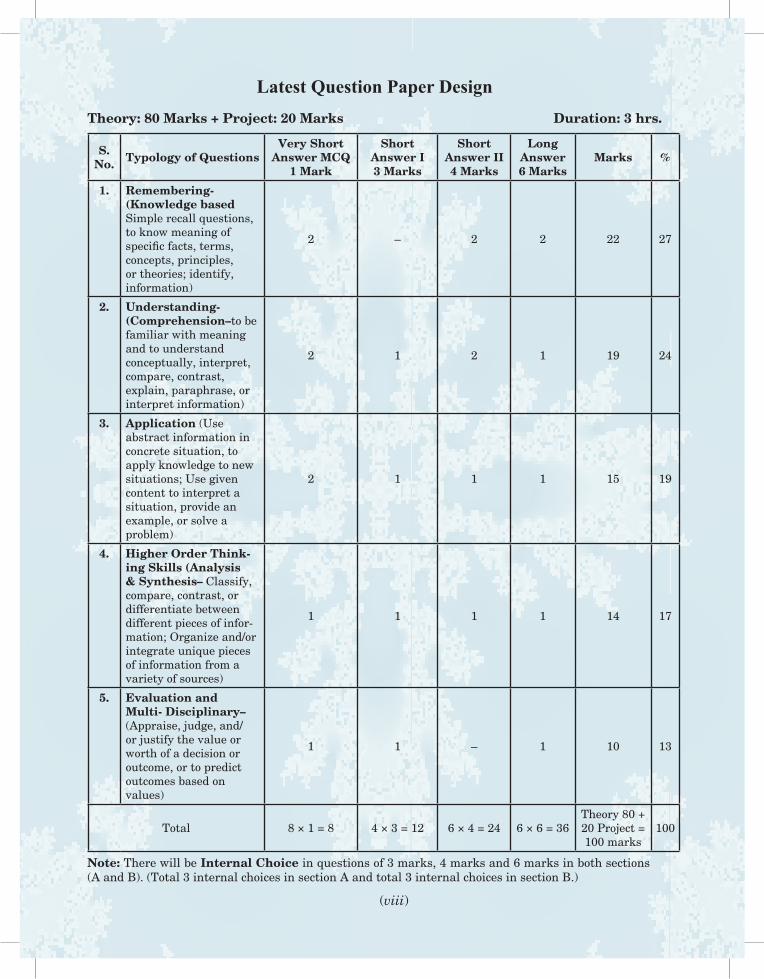
Latest Question Paper Design Theory: 80 Marks + Project: 20 Marks Duration: 3 hrs.
S.No. Typology of Questions
Very Short Answer MCQ
1 Mark
Short Answer I 3 Marks
Short Answer II 4 Marks
long Answer 6 Marks
Marks %
1. Remembering- (Knowledge based Simple recall questions, to know meaning of specific facts, terms, concepts, principles, or theories; identify, information)
2 – 2 2 22 27
2. Understanding- (Comprehension–to be familiar with meaning and to understand conceptually, interpret, compare, contrast, explain, paraphrase, or interpret information)
2 1 2 1 19 24
3. Application (Use abstract information in concrete situation, to apply knowledge to new situations; Use given content to interpret a situation, provide an example, or solve a problem)
2 1 1 1 15 19
4. Higher Order Think-ing Skills (Analysis & Synthesis– Classify, compare, contrast, or differentiate between different pieces of infor-mation; organize and/or integrate unique pieces of information from a variety of sources)
1 1 1 1 14 17
5. Evaluation and Multi- Disciplinary– (Appraise, judge, and/or justify the value or worth of a decision or outcome, or to predict outcomes based on values)
1 1 – 1 10 13
Total 8 × 1 = 8 4 × 3 = 12 6 × 4 = 24 6 × 6 = 36Theory 80 + 20 Project = 100 marks
100
Note: There will be Internal Choice in questions of 3 marks, 4 marks and 6 marks in both sections (A and B). (Total 3 internal choices in section A and total 3 internal choices in section B.)
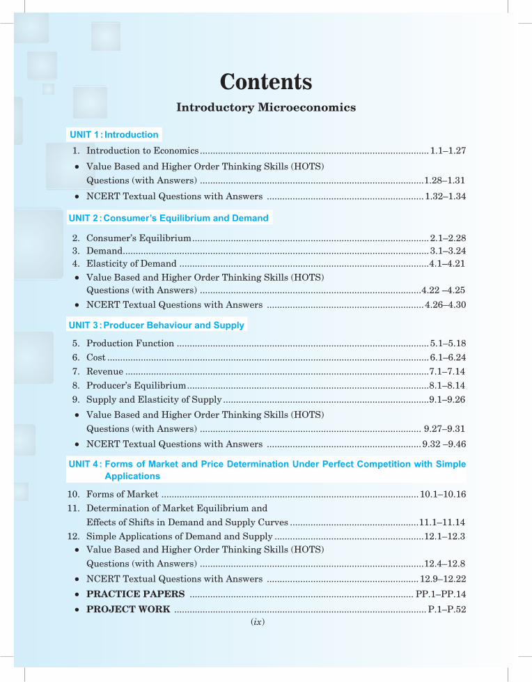
Contents
(ix)
Introductory Microeconomics
UNIT 1 : Introduction 1. Introduction to Economics .........................................................................................1.1–1.27
• Value Based and Higher Order Thinking Skills (HOTS) Questions (with Answers) .......................................................................................1.28–1.31
• NCERT Textual Questions with Answers .............................................................1.32–1.34
UNIT 2 : Consumer’s Equilibrium and Demand
2. Consumer’s Equilibrium ............................................................................................2.1–2.28 3. Demand .......................................................................................................................3.1–3.24 4. Elasticity of Demand .................................................................................................4.1–4.21 • Value Based and Higher Order Thinking Skills (HOTS) Questions (with Answers) ......................................................................................4.22 –4.25
• NCERT Textual Questions with Answers .............................................................4.26–4.30
UNIT 3 : Producer Behaviour and Supply
5. Production Function ..................................................................................................5.1–5.18 6. Cost .............................................................................................................................6.1–6.24 7. Revenue ......................................................................................................................7.1–7.14 8. Producer’s Equilibrium ..............................................................................................8.1–8.14 9. Supply and Elasticity of Supply ................................................................................9.1–9.26
• Value Based and Higher Order Thinking Skills (HOTS) Questions (with Answers) ...................................................................................... 9.27–9.31
• NCERT Textual Questions with Answers ............................................................9.32 –9.46
UNIT 4 : Forms of Market and Price Determination Under Perfect Competition with Simple Applications
10. Forms of Market ....................................................................................................10.1–10.16 11. Determination of Market Equilibrium and Effects of Shifts in Demand and Supply Curves ..................................................11.1–11.14 12. Simple Applications of Demand and Supply ..........................................................12.1–12.3 • Value Based and Higher Order Thinking Skills (HOTS) Questions (with Answers) .......................................................................................12.4–12.8
• NCERT Textual Questions with Answers ...........................................................12.9–12.22
• PractIce PaPers ....................................................................................... PP.1–PP.14
• Project Work .................................................................................................. P.1–P.52

Dedicated to the Memory of
my dear Parents

IntroductionUNIT–1
This Unit Contains1. Introduction to Economics
1.1 What Economics is all about?
The science of economics was born with the publication of Adam Smith’s An Inquiry into the Nature and Causes of Wealth of Nations in the year 1776. Adam Smith is known as the father of Economics. At its birth, the name of economics was ‘Political Economy’.Towards the end of the 19th century there was a definite change from use of word ‘Political Economy’ to ‘Economics’. The word ‘Economics’ was derived from two Greek words oikou (a house) and nomos (to manage). Thus, the word economics was used to mean home management with limited funds available in the most economical manner possible.Lionel Robbins defines economics as a science of scarcity. Prof. Robbins in his book Nature and Significance of Economic Science states, “Economics is the science which studies human behaviour as a relationship between ends and scarce means which have alternative uses”.Paul A. Samuelson defines economics as “the study of how men and society choose, with
Introduction toEconomics
Chapter Scheme1.5 Production Possibility Curve (PPC) 1.5.1 Production Possibility Set and Curve 1.5.2 Assumptions 1.5.3 Production Possibility Schedule and
Curve 1.5.4 Features of Production Possibility Curve 1.5.5 Shifts in Production Possibility Curve1.6 Opportunity Cost1.7 Production Possibility Curve and Economic Problems 1.7.1 Allocation of Resources—What to Produce and How much to Produce? 1.7.2 Full Utilisation of Resources 1.7.3 Economic Efficiency 1.7.4 Economic Growth Points to Remember Test Your Knowledge Answers to MCQs and Short Answer
Questions
1.1 What Economics is All About?1.2 Microeconomics and Macroeconomics 1.2.1 Subject–matter of Economics 1.2.2 Microeconomics—Meaning,
Subject–matter, Importance and Limitations
1.2.3 Macroeconomics—Meaning, Subject–matter, Importance and Limitations
1.2.4 Interdependence of Micro and Macro Economics
1.3 Positive and Normative Economics 1.3.1 Economics as a Positive Science 1.3.2 Economics as a Normative Science 1.3.3 Interdependence of Positive and Normative Science1.4 Economic Problems of an Economy 1.4.1 Economy: Meaning 1.4.2 Meaning of Economic Problems 1.4.3 Causes of Economic Problems 1.4.4 Economic Problems of an Economy
1
Saraswati Introductory Microeconomics1.2
or without the use of money, to employ scarce productive resources which could have alternative uses, to produce various commodities over time and distribute them for consumption now and in future among various people and groups of society.” This definition emphasises growth over time. It is modern and wider in scope. The definition takes into account consumption, production, distribution and exchange ofgoods. Hence, it is most satisfactory definition of economics. This definition has been accepted universally.
1.2 microEconomics and macroEconomics
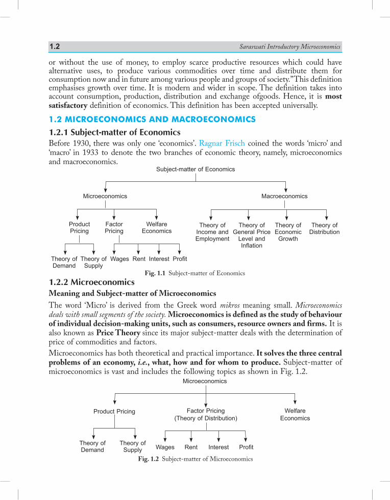
1.2.1 Subject-matter of EconomicsBefore 1930, there was only one ‘economics’. Ragnar Frisch coined the words ‘micro’ and ‘macro’ in 1933 to denote the two branches of economic theory, namely, microeconomics and macroeconomics.
1.2.2 MicroeconomicsMeaning and Subject-matter of MicroeconomicsThe word ‘Micro’ is derived from the Greek word mikros meaning small. Microeconomics deals with small segments of the society. Microeconomics is defined as the study of behaviour of individual decision-making units, such as consumers, resource owners and firms. It is also known as Price Theory since its major subject-matter deals with the determination of price of commodities and factors.Microeconomics has both theoretical and practical importance. It solves the three central problems of an economy, i.e., what, how and for whom to produce. Subject-matter of microeconomics is vast and includes the following topics as shown in Fig. 1.2.
Fig. 1.1 Subject-matter of Economics
Subject-matter of Economics
Microeconomics
ProductPricing
FactorPricing
WelfareEconomics
Macroeconomics
Theory ofDemand
Theory ofSupply
Wages Rent Interest Profit
Theory ofIncome andEmployment
Theory ofGeneral Price
Level andInflation
Theory ofEconomic
Growth
Theory ofDistribution
Fig. 1.2 Subject-matter of Microeconomics
Microeconomics
Product Pricing WelfareEconomics
Factor Pricing(Theory of Distribution)
Theory ofDemand
Theory ofSupply Wages Rent Interest Profit
Introduction to Economics 1.3
Importance of MicroeconomicsMicroeconomics has both theoretical and practical importance. It is clear from the following points:1. Microeconomics helps in formulating economic policies which enhance productive
efficiency and results in greater social welfare.2. Microeconomics explains the working of a capitalist economy where individual units
(i.e., producers and consumers) are free to take their own decision.3. Microeconomics describes how, in a free enterprise economy, individual units attain
equilibrium position.4. It helps the government in formulating correct price policies.5. It helps in efficient employment of resources by the entrepreneurs.6. It helps business economist to make conditional predictions and business forecasts.7. It is used to explain gains from trade, disequilibrium in the balance of payment position
and determination of international exchange rate.
Limitations of MicroeconomicsMicroeconomics fails to explain the functioning of an economy as a whole. It cannot explain unemployment, poverty, illiteracy and other problems prevailing in the country.
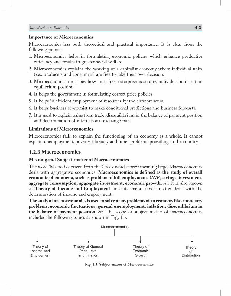
1.2.3 MacroeconomicsMeaning and Subject-matter of MacroeconomicsThe word ‘Macro’ is derived from the Greek word makros meaning large. Macroeconomics deals with aggregative economics. Macroeconomics is defined as the study of overall economic phenomena, such as problem of full employment, GNP, savings, investment, aggregate consumption, aggregate investment, economic growth, etc. It is also known as Theory of Income and Employment since its major subject-matter deals with the determination of income and employment.The study of macroeconomics is used to solve many problems of an economy like, monetary problems, economic fluctuations, general unemployment, inflation, disequilibrium in the balance of payment position, etc. The scope or subject-matter of macroeconomics includes the following topics as shown in Fig. 1.3.
Fig. 1.3 Subject-matter of Macroeconomics
Macroeconomics
Theory ofIncome andEmployment
Theory of GeneralPrice Leveland Inflation
Theory ofEconomic
Growth
Theoryof
Distribution
Saraswati Introductory Microeconomics1.4
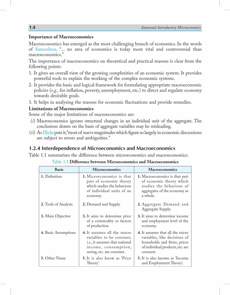
Importance of MacroeconomicsMacroeconomics has emerged as the most challenging branch of economics. In the words of Samuelson, “... no area of economics is today more vital and controversial than macroeconomics.” The importance of macroeconomics on theoretical and practical reasons is clear from the following points:1. It gives an overall view of the growing complexities of an economic system. It provides
powerful tools to explain the working of the complex economic systems.2. It provides the basic and logical framework for formulating appropriate macroeconomic
policies (e.g., for inflation, poverty, unemployment, etc.) to direct and regulate economy towards desirable goals.
3. It helps in analysing the reasons for economic fluctuations and provide remedies.Limitations of MacroeconomicsSome of the major limitations of macroeconomics are: (i) Macroeconomics ignores structural changes in an individual unit of the aggregate. The
conclusions drawn on the basis of aggregate variables may be misleading. (ii) As Hicks puts it,“most of macro magnitudes which figure so largely in economic discussions
are subject to errors and ambiguities.”
1.2.4 Interdependence of Microeconomics and MacroeconomicsTable 1.1 summarises the difference between microeconomics and macroeconomics.
Table 1.1 Difference between Microeconomics and Macroeconomics
Basis Microeconomics Macroeconomics
1. Definition 1. Microeconomics is that part of economic theory which studies the behaviour of individual units of an economy.
1. Macroeconomics is that part of economic theory which studies the behaviour of aggregates of the economy as a whole.
2. Tools of Analysis 2. Demand and Supply. 2. Aggregate Demand and Aggregate Supply.
3. Main Objective 3. It aims to determine price of a commodity or factors of production.
3. It aims to determine income and employment level of the economy.
4. Basic Assumptions 4. It assumes all the macro variables to be constant, i.e., it assumes that national income, consumpt ion, saving, etc. are constant.
4. It assumes that all the micro variables, like decisions of households and firms, prices of individual products, etc. are constant.
5. Other Name 5. It is also know as ‘Price Theory’.
5. It is also known as ‘Income and Employment Theory’.
Introduction to Economics 1.5
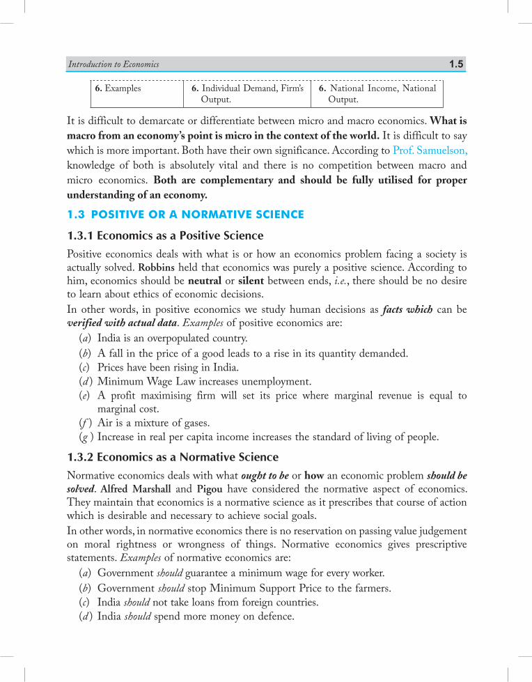
6. Examples 6. Individual Demand, Firm’s Output.
6. National Income, National Output.
It is difficult to demarcate or differentiate between micro and macro economics. What is macro from an economy’s point is micro in the context of the world. It is difficult to say which is more important. Both have their own significance. According to Prof. Samuelson, knowledge of both is absolutely vital and there is no competition between macro and micro economics. Both are complementary and should be fully utilised for proper understanding of an economy.
1.3 positivE or a normativE sciEncE
1.3.1 Economics as a Positive SciencePositive economics deals with what is or how an economics problem facing a society is actually solved. Robbins held that economics was purely a positive science. According to him, economics should be neutral or silent between ends, i.e., there should be no desire to learn about ethics of economic decisions.In other words, in positive economics we study human decisions as facts which can be verified with actual data. Examples of positive economics are: (a) India is an overpopulated country. (b) A fall in the price of a good leads to a rise in its quantity demanded. (c) Prices have been rising in India. (d ) Minimum Wage Law increases unemployment. (e) A profit maximising firm will set its price where marginal revenue is equal to
marginal cost. (f ) Air is a mixture of gases. (g ) Increase in real per capita income increases the standard of living of people.
1.3.2 Economics as a Normative ScienceNormative economics deals with what ought to be or how an economic problem should be solved. Alfred Marshall and Pigou have considered the normative aspect of economics. They maintain that economics is a normative science as it prescribes that course of action which is desirable and necessary to achieve social goals.In other words, in normative economics there is no reservation on passing value judgement on moral rightness or wrongness of things. Normative economics gives prescriptive statements. Examples of normative economics are: (a) Government should guarantee a minimum wage for every worker. (b) Government should stop Minimum Support Price to the farmers. (c) India should not take loans from foreign countries. (d ) India should spend more money on defence.
Saraswati Introductory Microeconomics1.6
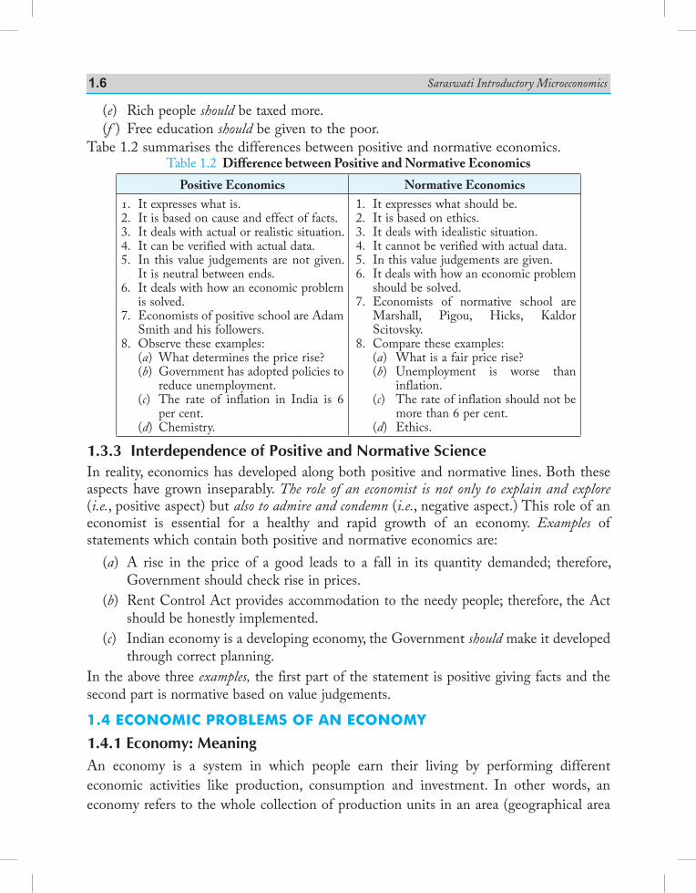
(e) Rich people should be taxed more. (f ) Free education should be given to the poor.Tabe 1.2 summarises the differences between positive and normative economics.
Table 1.2 Difference between Positive and Normative Economics
Positive Economics Normative Economics1. It expresses what is.2. It is based on cause and effect of facts.3. It deals with actual or realistic situation.4. It can be verified with actual data.5. In this value judgements are not given.
It is neutral between ends.6. It deals with how an economic problem
is solved.7. Economists of positive school are Adam
Smith and his followers.8. Observe these examples: (a) What determines the price rise? (b) Government has adopted policies to
reduce unemployment. (c) The rate of inflation in India is 6
per cent. (d) Chemistry.
1. It expresses what should be.2. It is based on ethics.3. It deals with idealistic situation.4. It cannot be verified with actual data.5. In this value judgements are given.6. It deals with how an economic problem
should be solved.7. Economists of normative school are
Marshall, Pigou, Hicks, Kaldor Scitovsky.
8. Compare these examples: (a) What is a fair price rise? (b) Unemployment is worse than
inflation. (c) The rate of inflation should not be
more than 6 per cent. (d) Ethics.
1.3.3 Interdependence of Positive and Normative ScienceIn reality, economics has developed along both positive and normative lines. Both these aspects have grown inseparably. The role of an economist is not only to explain and explore (i.e., positive aspect) but also to admire and condemn (i.e., negative aspect.) This role of an economist is essential for a healthy and rapid growth of an economy. Examples of statements which contain both positive and normative economics are: (a) A rise in the price of a good leads to a fall in its quantity demanded; therefore,
Government should check rise in prices. (b) Rent Control Act provides accommodation to the needy people; therefore, the Act
should be honestly implemented. (c) Indian economy is a developing economy, the Government should make it developed
through correct planning.In the above three examples, the first part of the statement is positive giving facts and the second part is normative based on value judgements.
1.4 Economic problEms of an Economy
1.4.1 Economy: MeaningAn economy is a system in which people earn their living by performing different economic activities like production, consumption and investment. In other words, an economy refers to the whole collection of production units in an area (geographical area
Introduction to Economics 1.7
or political boundary) of a country by which people get their living. An economy is classified into market economy and planned economy. These economies can be subdivided into closed economy and open economy.
1.4.2 Meaning of Economic Problems
Economic problem is the problem of choice. The problem of choice has to be faced by every economy of the world, whether developed or developing. Human beings have wants which are unlimited. When these wants get satisfied, new wants crop up. Human wants multiply at a fast rate. The economic resources to satisfy these unlimited wants are limited.In other words, resources or factors of production (they are defined as goods and services needed to carry out production i.e., land, labour, capital and entrepreneurship) are scarce. They are available in limited quantities in relation to the demand. Resources are not only scarce but they also have alternative uses. All this necessitates a choice between which goods and services to produce first. The economy comprising of individuals, business firms, and societies must make this choice.According to Prof. Robbins, “the economic problem is the problem of choice or the problem of economising, i.e., it is the problem of fuller and efficient utilisation of the limited resources to satisfy maximum number of wants. The scarcity of resources creates this situation.” If an economy employs more resources to produce good X, then it will have to forego the production of good Y. Hence, economy has to choose which of the two goods X or Y will give more satisfaction. An economy can produce both wheat and rice on the same plot of land. The decision to produce wheat is an outcome of choice.
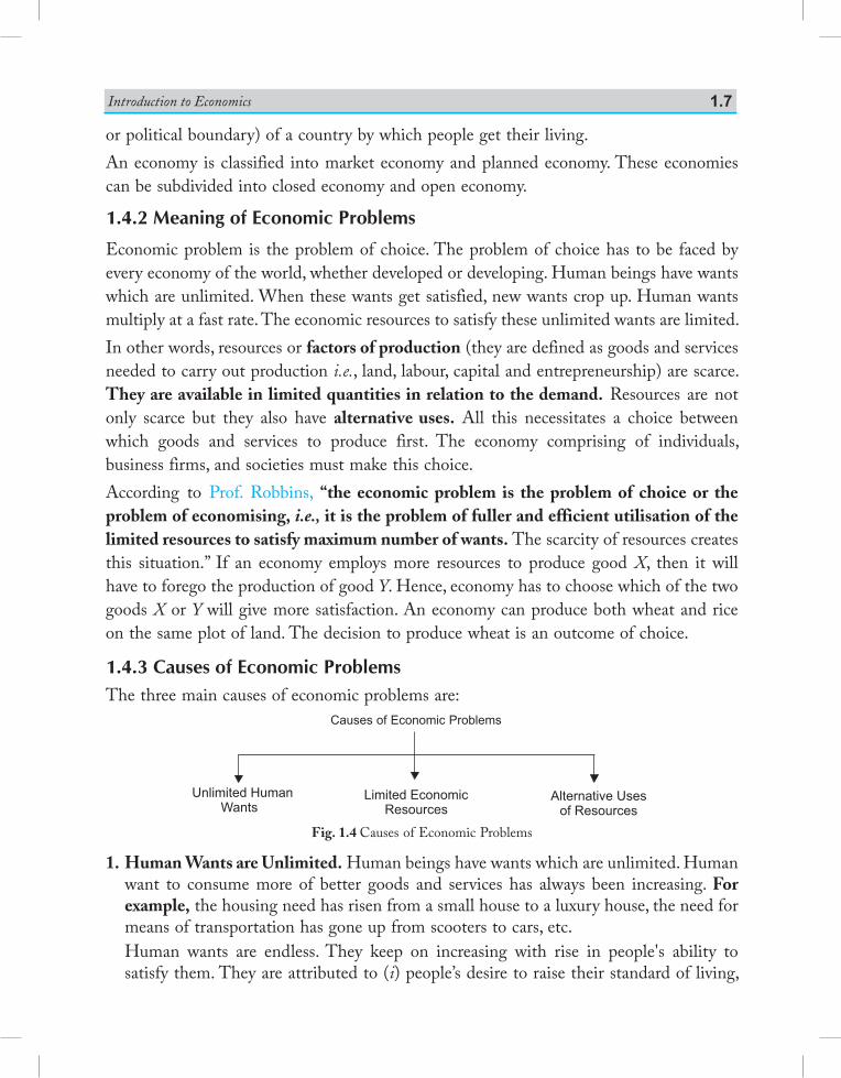
1.4.3 Causes of Economic ProblemsThe three main causes of economic problems are:
Fig. 1.4 Causes of Economic Problems
1. Human Wants are Unlimited. Human beings have wants which are unlimited. Human want to consume more of better goods and services has always been increasing. For example, the housing need has risen from a small house to a luxury house, the need for means of transportation has gone up from scooters to cars, etc.
Human wants are endless. They keep on increasing with rise in people's ability to satisfy them. They are attributed to (i) people’s desire to raise their standard of living,
Causes of Economic Problems
Saraswati Introductory Microeconomics1.8
comforts and efficiency; (ii) human tendency to accumulate things beyond their present need, (iii) multiplicative nature of some wants e.g. buying a car creates want for many other things - petrol, driver, car parking place, safety locks, spare parts, insurance, etc. (iv) basic needs for food, water and clothing, (v) influence of advertisements in modern times create new kinds of wants and demonstration effect. Due to these reasons human wants continue to increase endlessly.
While some wants have to be satisfied as and when they arise such as food, clothes, shelter, water, etc., some can be postponed e.g. purchase of a luxury car. The priority of wants varies from person to person and from time to time for the same person. Therefore, the question arises as to ‘which want to satisfy first’ and ‘which the last’. Thus, consumers have to make the choice as to ‘what to consume’ and ‘how much to consume’.
2. Resources are Limited. Scarcity of resources is the root cause of all economic problems. All resources that are available to the people at any point of time for satisfying their wants are scarce and limited. Conceptually, anything which is available and can be used to satisfy human wants and desire is a resource. In economics, however, resources that are available to individuals, households, firms and society at any point of time are traditionally natural resources (land). Human resources (labour), capital resources (like machine, building, etc.) and entrepreneurship are scarce. Resource scarcity is a relative term. It implies that resources are scarce in relation to the demand for resources. The scarcity of resources is the mother of all economic problems. It forces people to make choices.
3. Resources have Alternative Uses. Resources are not only scarce in supply but they have alternative uses. Same resources cannot be used for more than one purpose at a time. For example, ` 100 can be put in various alternative purposes such as buying petrol, notebook, ice-cream, burger, cold drink, etc. Similarly an area of land can be used for farming or as a playground or for constructing school, college or hospital building or for constructing residential building, etc. But return on the area of a land or utility of putting ` 100 in various uses varies according to the use of the concerned resources. Thus, people have to make choice between alternating uses of the resources. If the area of land is put to a particular use, the landlord has to forgo the return expected from its other alternative uses. This is termed as opportunity cost.
Economics as a social science analyses how people (individuals and the whole society or economy) make their choices between economic goals they want to achieve, between goods and services they want to produce and between alternative uses of their resources which will maximise their gains.
1.4.4 Economic Problems of an EconomyEconomic problems are reflected in the form of Central or Basic Problems of an economy. Any economy—whether market, centrally planned, or mixed—has to face these problems. According to Samuelson, there are three fundamental and interdependent problems in an economic organisation—what, how and for whom—which are grouped under allocation of
Introduction to Economics 1.9
resources. Allocation of resources means how much of each resource is devoted to the production of goods and services.1. Allocation of Resources
(a) What Goods to Produce and How Much to Produce? Due to limited resources, every economy has to decide what goods to produce and in what quantities. If the means were unlimited, then it would lead to a stage of salvation. But the means are limited and the economy must decide the efficient allocation of scarce resources so that both output and output-mix are optimum. An economy has to make a choice of the wants which are important for the economy as a whole. For example, if the economy decides to produce more cloth, it is bound to reduce the production of food. The reason is that resources used to produce food and cloth are limited and given. An economy cannot produce more of both food and cloth. Thus, an economy has to decide what goods it would produce on the basis of availability of technology, cost of production, cost of supplying and demand for the commodity.
(b) How to Produce? It is the question of choice of technique of production. Since resources are scarce, an inefficient technique of production, which would lead to wastage and high cost, cannot be applied. A technique of production which would maximise output or minimise cost should be used. We generally consider two types of techniques of production: labour-intensive and capital-intensive techniques. In labour-intensive technique, more labour and less capital is used. In capital-intensive technique, more capital and less labour is used.For example, it is always technically possible to produce a given amount of wheat or rice with more of labour and less of capital (i.e. with labour intensive technology) or with more of capital and less of labour (i.e. with capital intensive technology). The same is true for most commodities. In the case of some commodities however, choices are limited. For example, production of woollen carpets and other items of handicrafts is by nature labour intensive, while production of cars, TV sets, computers, aircrafts, etc., is capital intensive. In most commodities, however, alternative technology may be available. Alternative techniques of production involve varying costs. Therefore, the problem of choice of technology arises. The guiding principle of this problem is to adopt such technique of production which has least cost to produce per unit of the commodity. At macro level the most efficient technique is the one which uses least quantity of scarce resources.Hence, producers must always produce efficiently by using the most efficient technology. Thus, every economy has to choose the most efficient technique of producing a commodity.(c) For Whom to Produce? This is the question of how to distribute the product among the various sections of the society. National product is the total output generated by the firms. Goods and services are produced in the economy for those who have the ability (i.e. capacity) to buy them.
Saraswati Introductory Microeconomics1.10
Ability or capacity or purchasing power of people depends on their income. More income means more capacity to buy. The total output ultimately flows to the households in the form of income, i.e., their wages, rent, profits or interest. There are millions of people in a society. Each one cannot get sufficient income to satisfy all his wants. This raises the problem of distribution of national product among different households. Who should get how much is thus the problem? Thus, guiding principle of this problem is output of the economy be distributed among different sections of the society in such a way that all of them get a minimum level of consumption.1.5 production possibility curvE (ppc)
1.5.1 Production Possibility Set and CurveProduction possibility set refers to different possible combinations of two goods that can be produced from a given amount of resources and a given level of technology.Production possibility curve or frontier (PPF) shows the various alternative combinations of goods and services that an economy can produce when the resources are all fully and efficiently employed. PPC shows the obtainable options.There is a maximum limit to the amount of goods and services which an economy can produce with the given resources and the state of technology. The resources can be used to produce various alternative goods which are called production possibilities and the curve showing the different production possibilities is called production possibility curve.
1.5.2 AssumptionsAssumptions underlying production possibility curve are: (a) Economy produces only two goods, X and Y. (Examples of goods X and Y can be gun
and butter, wheat and sugar cane, cricket bats and tennis rackets or anything else.) (b) Amount of resources available in an economy are given and fixed. (c) Resources are not specific, i.e., they can be shifted from the production of one good
to the other good. (d ) Resources are fully employed, i.e., there is no wastage of resources. Resources are
not lying idle. (e) State of technology in an economy is given and remains unchanged. (f ) Resources are efficiently employed (efficiency in production means output per
unit of an input).1.5.3 Production Possibility Schedule and Curve PP schedule refers to tabular presentation of different possible combinations of two goods that an economy can produce with given resources and available technology. Table 1.3, gives a production possibility schedule. It shows that, with given resources, an economy can produce either zero unit of X and 21 units of Y or 1 of X and 20 of Y or 2 units of X and 18 units of Y or 3 units of X and 15 units of Y or 4 of X and 11 of Y or 5 of X and 6 of Y or 6 units of X and zero units of Y.
Introduction to Economics 1.11
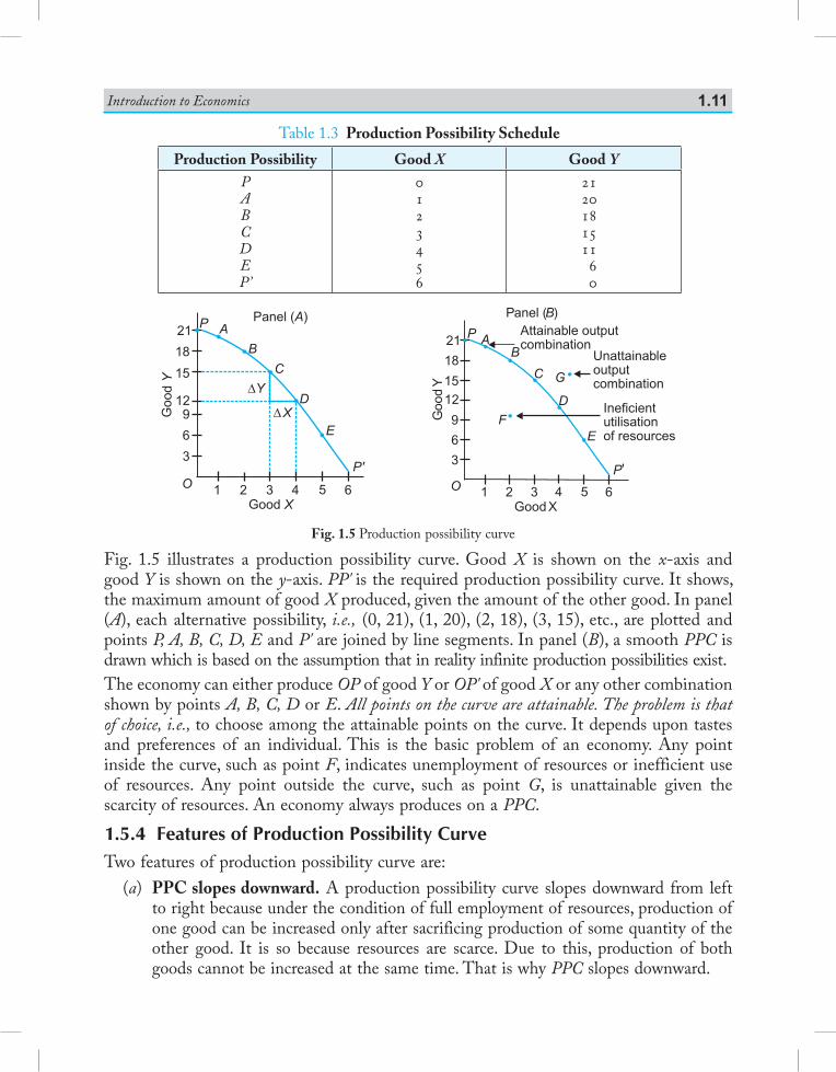
Table 1.3 Production Possibility Schedule
Production Possibility Good X Good YPABCDEP’
0123456
212018151160
Fig. 1.5 illustrates a production possibility curve. Good X is shown on the x-axis and good Y is shown on the y-axis. PP' is the required production possibility curve. It shows, the maximum amount of good X produced, given the amount of the other good. In panel (A), each alternative possibility, i.e., (0, 21), (1, 20), (2, 18), (3, 15), etc., are plotted and points P, A, B, C, D, E and P' are joined by line segments. In panel (B), a smooth PPC is drawn which is based on the assumption that in reality infinite production possibilities exist.The economy can either produce OP of good Y or OP' of good X or any other combination shown by points A, B, C, D or E. All points on the curve are attainable. The problem is that of choice, i.e., to choose among the attainable points on the curve. It depends upon tastes and preferences of an individual. This is the basic problem of an economy. Any point inside the curve, such as point F, indicates unemployment of resources or inefficient use of resources. Any point outside the curve, such as point G, is unattainable given the scarcity of resources. An economy always produces on a PPC.1.5.4 Features of Production Possibility Curve Two features of production possibility curve are: (a) PPC slopes downward. A production possibility curve slopes downward from left
to right because under the condition of full employment of resources, production of one good can be increased only after sacrificing production of some quantity of the other good. It is so because resources are scarce. Due to this, production of both goods cannot be increased at the same time. That is why PPC slopes downward.
21
18
1512
9
6
3
O 1 2 3 4 5 6
P A
Good X
B
C
E
P'
D
Goo
dY
FIneficientutilisationof resources
Panel ( )BAttainable outputcombination
G
Unattainableoutputcombination
Fig. 1.5 Production possibility curve
Saraswati Introductory Microeconomics1.12
(b) PPC is concave to the origin. A production possibility curve is concave to the point of origin because of increasing marginal rate of transformation (MRT) or increasing marginal opportunity cost (MOC). Slope of PPC is defined as the quantity of good Y given up in exchange for additional unit of good X.
[Slope of Production Possibility Curve] = DYDX
= Amount of Good Y lostAmount of Good X gained
= MRT or [Marginal Opportunity Cost]
Marginal opportunity cost is opportunity cost of good X gained in terms of good Y given up. It is also called Marginal Rate of Transformation (MRT).
Concave shape of PPC means that slope of PPC increase which implies that MRT increases. It means that for producing an additional unit of a good, sacrifice of units of other good (i.e. opportunity cost) goes on increasing. It is because resources are not equally efficient for the production of both goods. Thus, if resources are transferred from production of one good to another, cost increases i.e., MRT or MOC increases. It is called law of increasing opportunity cost.
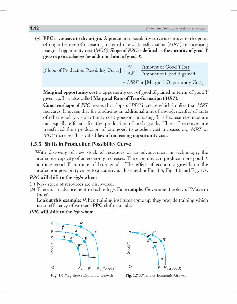
1.5.5 Shifts in Production Possibility Curve With discovery of new stock of resources or an advancement in technology, the
productive capacity of an economy increases. The economy can produce more good X or more good Y or more of both goods. The effect of economic growth on the production possibility curve to a country is illustrated in Fig. 1.5, Fig. 1.6 and Fig. 1.7.
PPC will shift to the right when:(a) New stock of resources are discovered.(b) There is an advancement in technology. For example: Government policy of ‘Make in
India’. Look at this example: When training institutes come up, they provide training which
raises efficiency of workers. PPC shifts outside.PPC will shift to the left when:
Fig. 1.6 P1P ’1 shows Economic GrowthGood X
B
A'
A
GoodY
P 1
P2
P
P 1'P 2' P'O
B'A''
B''
Fig. 1.7 PP1 shows Economic Growth
Good X
B
B'
A'
A
Goo
dY
P
O P1P'
Introduction to Economics 1.13
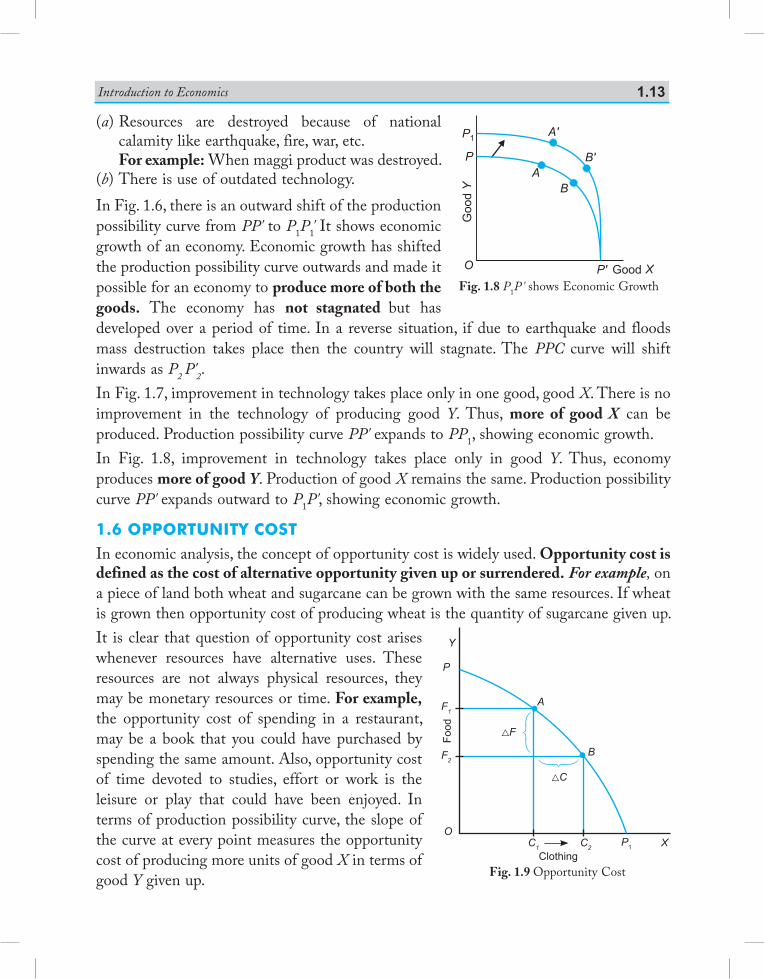
(a) Resources are destroyed because of national calamity like earthquake, fire, war, etc.
For example: When maggi product was destroyed.(b) There is use of outdated technology.In Fig. 1.6, there is an outward shift of the production possibility curve from PP' to P1P1' It shows economic growth of an economy. Economic growth has shifted the production possibility curve outwards and made it possible for an economy to produce more of both the goods. The economy has not stagnated but has developed over a period of time. In a reverse situation, if due to earthquake and floods mass destruction takes place then the country will stagnate. The PPC curve will shift inwards as P2 P'2.In Fig. 1.7, improvement in technology takes place only in one good, good X. There is no improvement in the technology of producing good Y. Thus, more of good X can be produced. Production possibility curve PP' expands to PP1, showing economic growth.In Fig. 1.8, improvement in technology takes place only in good Y. Thus, economy produces more of good Y. Production of good X remains the same. Production possibility curve PP' expands outward to P1P', showing economic growth.
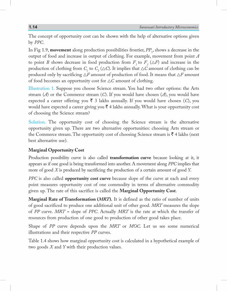
1.6 opportunity costIn economic analysis, the concept of opportunity cost is widely used. Opportunity cost is defined as the cost of alternative opportunity given up or surrendered. For example, on a piece of land both wheat and sugarcane can be grown with the same resources. If wheat is grown then opportunity cost of producing wheat is the quantity of sugarcane given up.It is clear that question of opportunity cost arises whenever resources have alternative uses. These resources are not always physical resources, they may be monetary resources or time. For example, the opportunity cost of spending in a restaurant, may be a book that you could have purchased by spending the same amount. Also, opportunity cost of time devoted to studies, effort or work is the leisure or play that could have been enjoyed. In terms of production possibility curve, the slope of the curve at every point measures the opportunity cost of producing more units of good X in terms of good Y given up.
Food
Clothing
O
F2
F1
C1 C2 P1 X
P
A
B
F
C
Y
Fig. 1.9 Opportunity Cost
Fig. 1.8 P1P' shows Economic GrowthGood X
B
B'
A'
A
Good
Y
P1
P
P'O
Saraswati Introductory Microeconomics1.14
The concept of opportunity cost can be shown with the help of alternative options given by PPC.In Fig 1.9, movement along production possibilities frontier, PP1, shows a decrease in the output of food and increase in output of clothing. For example, movement from point A to point B shows decrease in food production from F1 to F2 (F) and increase in the production of clothing from C1 to C2 (C). It implies that C amount of clothing can be produced only by sacrificing F amount of production of food. It means that F amount of food becomes an opportunity cost for C amount of clothing.Illustration 1. Suppose you choose Science stream. You had two other options: the Arts stream (A) or the Commerce stream (C). If you would have chosen (A), you would have expected a career offering you ` 3 lakhs annually. If you would have chosen (C), you would have expected a career giving you ` 4 lakhs annually. What is your opportunity cost of choosing the Science stream?
Solution. The opportunity cost of choosing the Science stream is the alternative opportunity given up. There are two alternative opportunities: choosing Arts stream or the Commerce stream. The opportunity cost of choosing Science stream is ` 4 lakhs (next best alternative use).
Marginal Opportunity Cost
Production possibility curve is also called transformation curve because looking at it, it appears as if one good is being transformed into another. A movement along PPC implies that more of good X is produced by sacrificing the production of a certain amount of good Y.
PPC is also called opportunity cost curve because slope of the curve at each and every point measures opportunity cost of one commodity in terms of alternative commodity given up. The rate of this sacrifice is called the Marginal Opportunity Cost.
Marginal Rate of Transformation (MRT). It is defined as the ratio of number of units of good sacrificed to produce one additional unit of other good. MRT measures the slope of PP curve. MRT = slope of PPC. Actually MRT is the rate at which the transfer of resources from production of one good to production of other good takes place.
Shape of PP curve depends upon the MRT or MOC. Let us see some numerical illustrations and their respective PP curves.
Table 1.4 shows how marginal opportunity cost is calculated in a hypothetical example of two goods X and Y with their production values.

Introduction to Economics 1.15
Table 1.4 Marginal Opportunity Cost along a PPC
Production of Good X Production of Good Y MRT =
MOC
012345
20191714105
—1Y : 1X2Y : 1X3Y : 1X4Y : 1X5Y : 1X
—12345
The table shows that, if the production of good X increases from 1 unit to 2 units, then two units of good Y (19 – 17) have to be foregone. Thus, marginal opportunity cost of good X is equal to 2 units of good Y. In the same way, marginal opportunity cost for other situations can be worked out. It is clear from the table that marginal opportunity cost increases from 1 to 2, 2 to 3, 3 to 4 and 4 to 5. It shows the law of increasing marginal opportunity cost. It’s economic meaning is that to produce one more unit of good X, increasing units of good Y have to be sacrificed.Illustration 2. An economy produces two goods, T-shirts and Cellphones. The following table summarises its production possibilities. Calculate the marginal opportunity cost of T-shirt at various combinations.
T-shirts (in millions) Cellphones (in thousands)012345
90,00080,00068,00052,00034,00010,000
Solution.Marginal Opportunity Cost
T-shirts (in millions)
(T)
Cellphones (in thousands)
(C)
Marginal Opportunity Cost of T-shirts (in Cellphones) = MRT
∆∆
∆∆
in good given upin good gained
in Cellphonesin T-shirt
=ss
012345
90,00080,00068,00052,00034,00010,000
—10,000 C : 1T12,000 C : 1T16,000 C : 1T18,000 C : 1T24,000 C : 1T
DYDX
Saraswati Introductory Microeconomics1.16
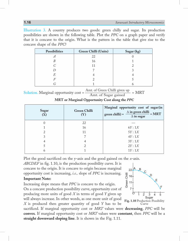
Illustration 3. A country produces two goods: green chilly and sugar. Its production possibilities are shown in the following table. Plot the PPC on a graph paper and verify that it is concave to the origin. What is the pattern in the table that give rise to the concave shape of the PPC?
Possibilities Green Chilli (Units) Sugar (kg)ABCDEFG
2216117421
0123456
Solution. Marginal opportunity cost = Amt. of Green Chilli given up Amt. of Sugar gained = MRT
MRT or Marginal Opportunity Cost along the PPC
Sugar(X)
Green Chilli(Y )
Marginal opportunity cost of sugar (in
green chilli) = D in green chilli
D in sugar = MRT
0123456
2216117421
—6Y : 1X5Y : 1X4Y : 1X3Y : 1X2Y : 1X1Y : 1X
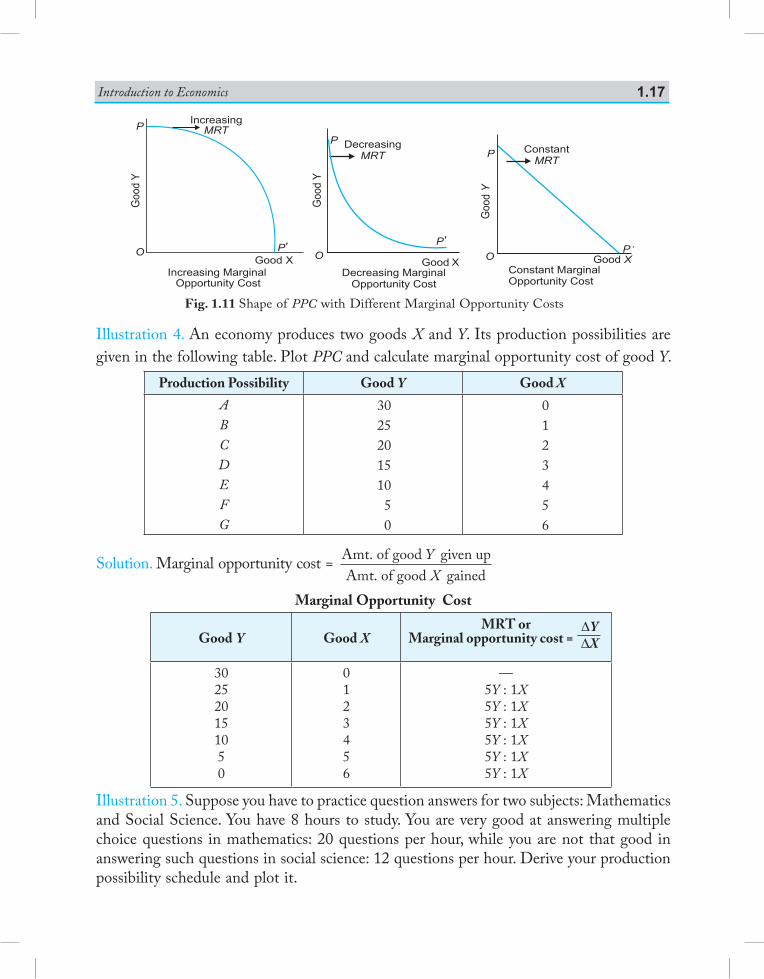
Plot the good sacrificed on the y-axis and the good gained on the x-axis.ABCDEF in fig. 1.10, is the production possibility curve. It is concave to the origin. It is concave to origin because marginal opportunity cost is increasing, i.e., slope of PPC is increasing. Important Note:Increasing slope means that PPC is concave to the origin.On a concave production possibility curve, opportunity cost of producing more units of good X in terms of good Y given up will always increase. In other words, as one more unit of good X is produced then greater quantity of good Y has to be sacrificed. If marginal opportunity cost or MRT values were decreasing, PPC will be convex. If marginal opportunity cost or MRT values were constant, then PPC will be a straight downward sloping line. It is shown in the Fig. 1.11.
Fig. 1.10 Production Possibility Curve
Introduction to Economics 1.17
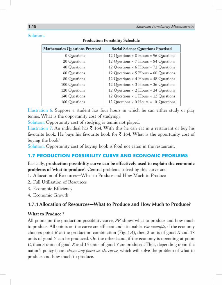
Illustration 4. An economy produces two goods X and Y. Its production possibilities are given in the following table. Plot PPC and calculate marginal opportunity cost of good Y.
Production Possibility Good Y Good X
ABCDEFG
302520151050
0123456
Solution. Marginal opportunity cost = Amt. of good given upAmt. of good gained
YX
Marginal Opportunity Cost
Good Y Good XMRT or
Marginal opportunity cost = DYDX
302520151050
0123456
—5Y : 1X5Y : 1X5Y : 1X5Y : 1X5Y : 1X5Y : 1X
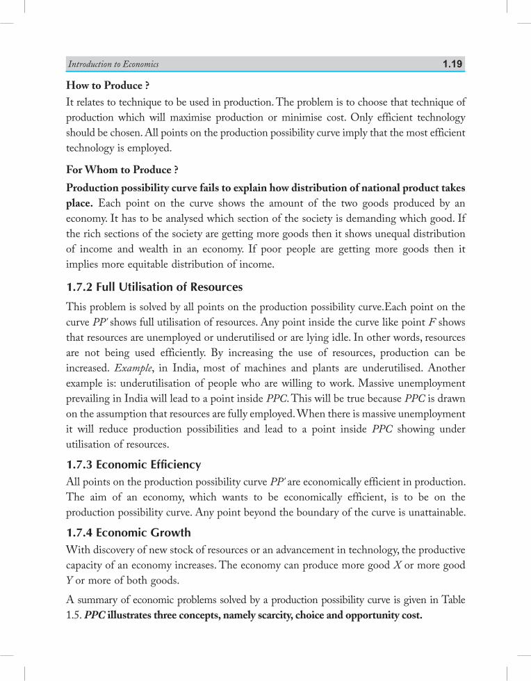
Illustration 5. Suppose you have to practice question answers for two subjects: Mathematics and Social Science. You have 8 hours to study. You are very good at answering multiple choice questions in mathematics: 20 questions per hour, while you are not that good in answering such questions in social science: 12 questions per hour. Derive your production possibility schedule and plot it.
Fig. 1.11 Shape of PPC with Different Marginal Opportunity Costs
Saraswati Introductory Microeconomics1.18
Solution.Production Possibility Schedule
Mathematics Questions Practised Social Science Questions Practised
0 Questions 20 Questions 40 Questions 60 Questions 80 Questions 100 Questions 120 Questions 140 Questions 160 Questions
12 Questions × 8 Hours = 96 Questions12 Questions × 7 Hours = 84 Questions12 Questions × 6 Hours = 72 Questions12 Questions × 5 Hours = 60 Questions12 Questions × 4 Hours = 48 Questions12 Questions × 3 Hours = 36 Questions12 Questions × 2 Hours = 24 Questions12 Questions × 1 Hours = 12 Questions12 Questions × 0 Hours = 0 Questions
Illustration 6. Suppose a student has four hours in which he can either study or play tennis. What is the opportunity cost of studying?Solution. Opportunity cost of studying is tennis not played.Illustration 7. An individual has ` 164. With this he can eat in a restaurant or buy his favourite book. He buys his favourite book for ` 164. What is the opportunity cost of buying the book?Solution. Opportunity cost of buying book is food not eaten in the restaurant.
1.7 production possibility curvE and Economic problEms
Basically, production possibility curve can be effectively used to explain the economic problems of ‘what to produce’. Central problems solved by this curve are:1. Allocation of Resources—What to Produce and How Much to Produce2. Full Utilisation of Resources3. Economic Efficiency4. Economic Growth
1.7.1 Allocation of Resources—What to Produce and How Much to Produce?
What to Produce ?All points on the production possibility curve, PP' shows what to produce and how much to produce. All points on the curve are efficient and attainable. For example, if the economy chooses point B as the production combination (Fig. 1.4), then 2 units of good X and 18 units of good Y can be produced. On the other hand, if the economy is operating at point C, then 3 units of good X and 15 units of good Y are produced. Thus, depending upon the nation’s policy it can choose any point on the curve, which will solve the problem of what to produce and how much to produce.
Introduction to Economics 1.19
How to Produce ?It relates to technique to be used in production. The problem is to choose that technique of production which will maximise production or minimise cost. Only efficient technology should be chosen. All points on the production possibility curve imply that the most efficient technology is employed.
For Whom to Produce ?
Production possibility curve fails to explain how distribution of national product takes place. Each point on the curve shows the amount of the two goods produced by an economy. It has to be analysed which section of the society is demanding which good. If the rich sections of the society are getting more goods then it shows unequal distribution of income and wealth in an economy. If poor people are getting more goods then it implies more equitable distribution of income.
1.7.2 Full Utilisation of Resources
This problem is solved by all points on the production possibility curve.Each point on the curve PP' shows full utilisation of resources. Any point inside the curve like point F shows that resources are unemployed or underutilised or are lying idle. In other words, resources are not being used efficiently. By increasing the use of resources, production can be increased. Example, in India, most of machines and plants are underutilised. Another example is: underutilisation of people who are willing to work. Massive unemployment prevailing in India will lead to a point inside PPC. This will be true because PPC is drawn on the assumption that resources are fully employed. When there is massive unemployment it will reduce production possibilities and lead to a point inside PPC showing under utilisation of resources.
1.7.3 Economic EfficiencyAll points on the production possibility curve PP' are economically efficient in production. The aim of an economy, which wants to be economically efficient, is to be on the production possibility curve. Any point beyond the boundary of the curve is unattainable.
1.7.4 Economic GrowthWith discovery of new stock of resources or an advancement in technology, the productive capacity of an economy increases. The economy can produce more good X or more good Y or more of both goods.
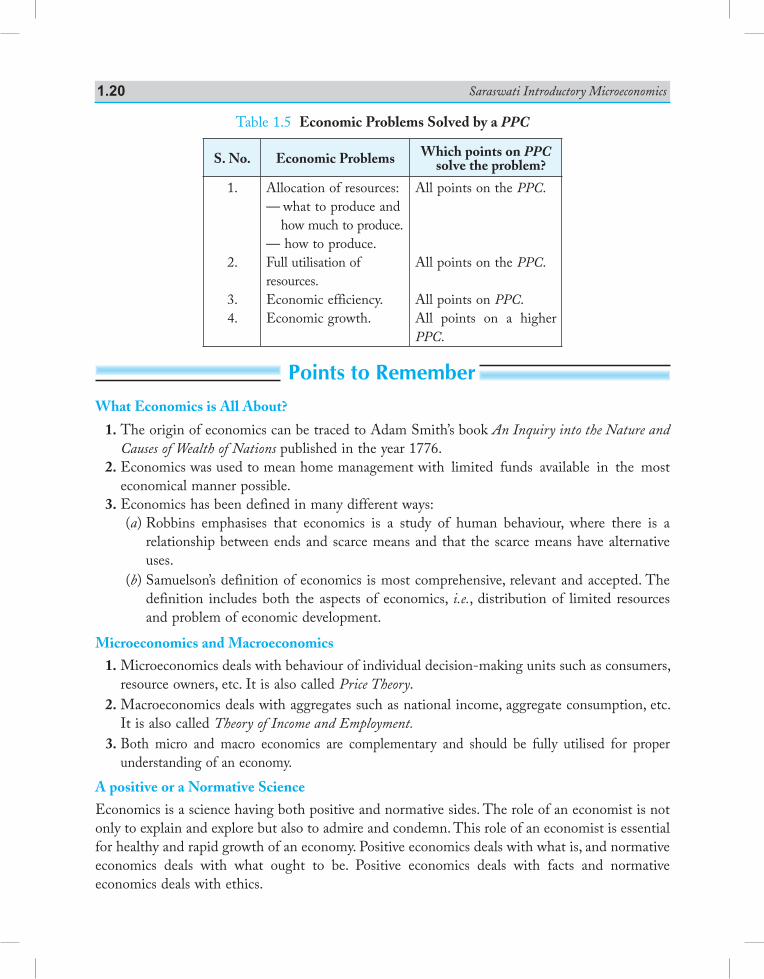
A summary of economic problems solved by a production possibility curve is given in Table 1.5. PPC illustrates three concepts, namely scarcity, choice and opportunity cost.
Saraswati Introductory Microeconomics1.20
Table 1.5 Economic Problems Solved by a PPC
S. No. Economic Problems Which points on PPC solve the problem?
1.
2.
3.4.
Allocation of resources:— what to produce and how much to produce.— how to produce.Full utilisation ofresources.Economic efficiency.Economic growth.
All points on the PPC.
All points on the PPC.
All points on PPC.All points on a higher PPC.
Points to RememberWhat Economics is All About?
1. The origin of economics can be traced to Adam Smith’s book An Inquiry into the Nature and Causes of Wealth of Nations published in the year 1776.
2. Economics was used to mean home management with limited funds available in the most economical manner possible.
3. Economics has been defined in many different ways: (a) Robbins emphasises that economics is a study of human behaviour, where there is a
relationship between ends and scarce means and that the scarce means have alternative uses.
(b) Samuelson’s definition of economics is most comprehensive, relevant and accepted. The definition includes both the aspects of economics, i.e., distribution of limited resources and problem of economic development.
Microeconomics and Macroeconomics
1. Microeconomics deals with behaviour of individual decision-making units such as con sum ers, resource owners, etc. It is also called Price Theory.
2. Macroeconomics deals with aggregates such as national income, aggregate con sump tion, etc. It is also called Theory of Income and Employment.
3. Both micro and macro economics are complementary and should be fully utilised for proper understanding of an economy.
A positive or a Normative Science
Economics is a science having both positive and normative sides. The role of an economist is not only to explain and explore but also to admire and condemn. This role of an economist is essential for healthy and rapid growth of an economy. Positive economics deals with what is, and normative economics deals with what ought to be. Positive economics deals with facts and normative economics deals with ethics.
Introduction to Economics 1.21
Economic Problems of an Economy
1. Basic economic problem is the problem of choice which is created by the scarcity of resources. It is also called problem of economising the resources, i.e., the problem of fuller and efficient utilisation of the limited resources to satisfy maximum number of wants.
2. Main causes of central problems are unlimited human wants, limited economic resources and alternative uses of resources.
3. Resources or factors of production can be natural like (land, air), human (i.e., labour), capital (like machines, building) and entrepreneurial (i.e., a person who bears risk).
4. Economic problems facing every economy are:Allocation of resources
(i) What to produce and how much to produce? (ii) How to produce? (iii) For whom to produce?Production Possibility Curve and Opportunity Cost
1. It is a useful device to graphically explain the central problems of an economy. It indicates the various combinations of goods and services which can be produced by full and efficient utilisation of all resources of an economy.
2. It is downward sloping concave to the origin curve.
3. Slope of PPC is called MRT or Marginal Opportunity Cost. Slope of PPC is increasing showing that if a country wants to produce more of good X it has to give up increasing number of units of good Y. It is called law of increasing marginal opportunity cost.
4. Any point inside the curve shows inefficent utilisation of resources and any point outside the curve is unattainable because of scarcity of resources.
5. Opportunity cost is the cost of alternative opportunity given up. Production possibility curve is called opportunity cost curve because slope of the curve at every point measures opportunity cost of good X in terms of good Y given up. On a convex PPC, marginal opportunity cost values are decreasing as MRT is decreasing. On a straight downward sloping PPC, MRT is constant.
Production Possibility Curve and Economic Problems
The production possibility curve solves five problems—what and how much to produce, how to produce, full utilisation of resources, economic efficiency and economic growth. All points on the curve solve the problems of what and how much to produce, how to produce, full employment of resources and economic efficiency. If the production possibility curve shifts outwards, it implies economic growth due to more production. Production possibility curve is unable to solve the economic problem of ‘for whom to produce’.
Saraswati Introductory Microeconomics1.22
Test Your KnowledgeVery Short Answer Type Questions (1 Mark)
1. What is economics? 2. Define central problems of an economy. 3. Which branch of economics deals with the problems of economic growth, economic
efficiency and full utilisation of re sourc es? 4. Define production possibility curve. (AI 2012) 5. What is opportunity cost? (Delhi 2012, Foreign 2013) 6. What does a leftward shift of production possibility curve indicate? 7. Define microeconomics. (AI 2012; Delhi 2012; Foreign 2011) 8. Define macroeconomics. (AI 2011; Foreign 2012) 9. Give one point of difference between micro and macro economics. 10. A teacher can do three job—teaching, tuition work and writing books. He gets ` 1 lakh from
teaching, ` 1.5 lakh from tuition work and ` 3 lakh from royalty of books. He is presently writing books. What is the opportunity cost of writing books?
11. Define an economy. (AI 2011; Delhi 2012) *12. Unemployment is reduced due to the measures taken by the government. State its economic
value in the context of production possibilities frontier. (Delhi 2014) *13. Th e government has started promoting foreign capital. What is its economic value in the
context of production possibilities frontier? (AI 2014) *14. Large number of technical training institutions have been started by the government. State
its economic value in the context of production possibilities frontier. (Foreign 2014)
Multiple Choice Questions
1. Who wrote ‘Nature and Causes of Wealth of Nations’? (a) Adam Smith (b) Alfred Marshall (c) Samuelson (d) Robbins 2. Price theory deals with: (a) Product pricing (b) Factor pricing (c) Welfare economics (d) All of the above 3. Macro economics deals with: (a) Theory of distribution (b) Theory of income and employment (c) theory of economic growth (d) All of the above 4. Economic problem arises because: (a) Wants are unlimited (b) Resources are scarce (c) Alternative uses of resources exist (d) All of the above
*Please see the answer at the end of exercises.
Introduction to Economics 1.23
5. Central problem of an economy can be: (a) What goods to produce and how much to produce (b) How to produce (c) For whom to produce (d) All of the above 6. Theory of distribution studies the problem of: (a) What goods to produce and how much to produce (b) How to produce (c) For whom to produce (d) All of the above 7. Theory of production studies the problem of (a) What goods to produce and how much to produce (b) How to produce (c) For whom to produce (d) All of the above 8. Price theory studies the problem of: (a) What goods to produce and how much to produce (b) How to produce (c) For whom to produce (d) All of the above 9. Production possibility curve (PPC) is defined as different combination of goods and services
that can be produced by whom when the resources are fully employed? (a) Firm (b) Industry (c) Economy (d) All of the above 10. Assumption of PPC is/are: (a) There are only two goods (b) Resources are not specific (c) Resources are fully employed (d) All of the above 11. Shape of PPC is: (a) Downward slopping concave to the origin (b) Downward sloping convex to the origin (c) Downward sloping straight line to the origin (d) All of the above 12. Smooth PPC is based on the assumption that: (a) Infinite production possibilities exist (b) Limited production possibilities exist (c) Two production possibilities exist (d) None of the above 13. PPC is also called: (a) Opportunity cost curve (b) Transformation curve (c) Production possibility frontier (d) All of the above
Saraswati Introductory Microeconomics1.24
14. If production of good X rises by 1 unit and that of good Y falls from 15 to 12.5 units then, marginal opportunity cost of X is:
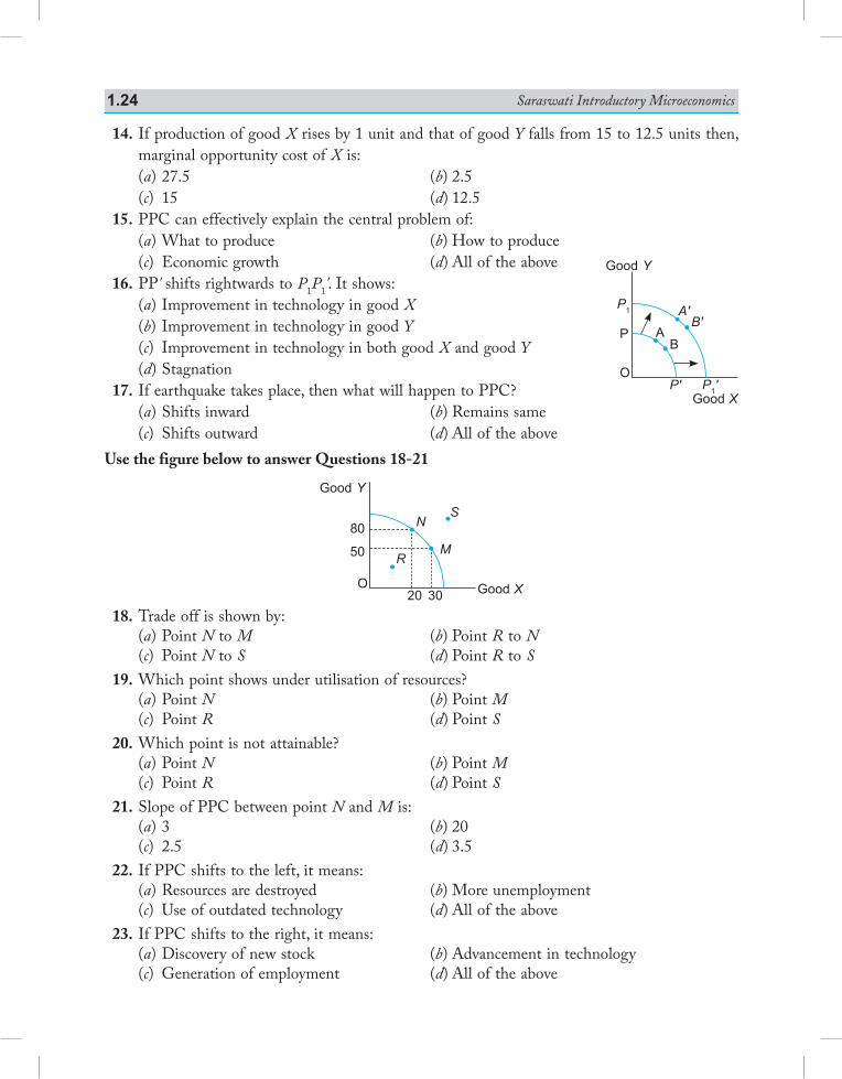
(a) 27.5 (b) 2.5 (c) 15 (d) 12.5 15. PPC can effectively explain the central problem of: (a) What to produce (b) How to produce (c) Economic growth (d) All of the above 16. PP' shifts rightwards to P1P1'. It shows: (a) Improvement in technology in good X (b) Improvement in technology in good Y (c) Improvement in technology in both good X and good Y (d) Stagnation 17. If earthquake takes place, then what will happen to PPC? (a) Shifts inward (b) Remains same (c) Shifts outward (d) All of the above Use the figure below to answer Questions 18-21
Good XO20
80
50
30
N
MR
S
Good Y
18. Trade off is shown by: (a) Point N to M (b) Point R to N (c) Point N to S (d) Point R to S 19. Which point shows under utilisation of resources? (a) Point N (b) Point M (c) Point R (d) Point S 20. Which point is not attainable? (a) Point N (b) Point M (c) Point R (d) Point S 21. Slope of PPC between point N and M is: (a) 3 (b) 20 (c) 2.5 (d) 3.5 22. If PPC shifts to the left, it means: (a) Resources are destroyed (b) More unemployment (c) Use of outdated technology (d) All of the above 23. If PPC shifts to the right, it means: (a) Discovery of new stock (b) Advancement in technology (c) Generation of employment (d) All of the above
Good X
O
P AB
P1
P1'P'
A'B'
Good Y
Introduction to Economics 1.25
Short Answer Type Questions (3/4 Marks)
1. Explain the problem of allocation of resources faced by an economy. 2. What does a production possibility curve show? 3. What is the effect of economic growth on a production possibility curve? 4. What does micro economics deal with? Give examples. 5. Distinguish between micro economics and macro economics. 6. Identify which of the following are the subject-matter of micro economics or macro
economics: (i) National Income, (ii) Supply by a firm, (iii) Cotton textile, (iv) Government budget, (v) Price determination of a commodity, (vi) Employment. 7. Explain the central problem of “how to produce”. (Foreign 2009) (AI 2009) 8. How can a production possibility curve solve economic problems faced by an economy? 9. Why is production possibility curve called the opportunity cost curve? 10. What is opportunity cost? Explain with the help of an example. (AI 2012) 11. (a) Suppose a student has four hours in which he can either study or play tennis. What is
the opportunity cost of studying? (c) An individual has ` 164. With this he can eat in a restaurant or buy his favourite book.
He buys his favourite book for ` 164. What is the opportunity cost of buying the book?
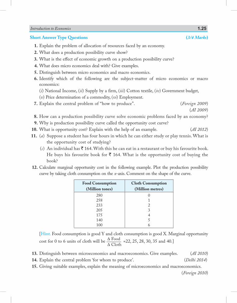
12. Calculate marginal opportunity cost in the following example. Plot the production possibility curve by taking cloth consumption on the x-axis. Comment on the shape of the curve.
Food Consumption(Million tones)
Cloth Consumption(Million metres)
280258233205175140100
0123456
[Hint. Food consumption is good Y and cloth consumption is good X. Marginal opportunity cost for 0 to 6 units of cloth will be D Food
D Cloth =22, 25, 28, 30, 35 and 40.]
13. Distinguish between microeconomics and macroeconomics. Give examples. (AI 2010) 14. Explain the central problem ‘for whom to produce’. (Delhi 2014) 15. Giving suitable examples, explain the meaning of microeconomics and macroeconomics. (Foreign 2010)
Saraswati Introductory Microeconomics1.26
16. Why is a production possibilities curve concave? Explain.(Delhi 2011; AI 2014) (Foreign 2012)
17. How is production possibility curve affected by unemployment in the economy? Explain. (AI 2011) 18. Explain how a production possibility curve is affected when resources are inefficiently
employed in an economy. (Foreign 2011) 19. Define Production Possibilities Curve. Explain why it is downward sloping from left to right. (AI, Foreign 2012, Foreign 2014) 20. What is ‘Marginal Rate of Transformation’? Explain with the help of an example. (Delhi, Foreign 2012) 21. State reasons why does an economic problem arise. (Delhi 2012) 22. Explain the central problem of ‘how to produce’. (AI 2012) 23. Define an economy. Why does it face the problem of ‘what to produce’? (Delhi 2012)
or Define an economy. Why does it face the problem of ‘how to produce’?
(AI 2012, Foreign 2013) 24. Production in an economy is below its potential due to unemployment. Government starts
employment generation schemes. Explain its effect using production possibilities curve. (Delhi 2013) 25. Explain the meaning of opportunity cost with the help of production possibility schedule.
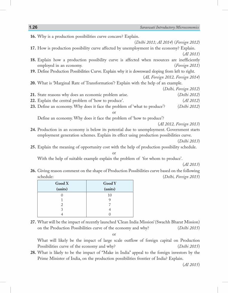
or With the help of suitable example explain the problem of ‘for whom to produce’. (AI 2013) 26. Giving reason comment on the shape of Production Possibilities curve based on the following
schedule: (Delhi, Foreign 2015)Good X(units)
Good Y(units)
01234
109740
27. What will be the impact of recently launched ‘Clean India Mission’ (Swachh Bharat Mission) on the Production Possibilities curve of the economy and why? (Delhi 2015)
or What will likely be the impact of large scale outflow of foreign capital on Production
Possibilities curve of the economy and why? (Delhi 2015) 28. What is likely to be the impact of “Make in India” appeal to the foreign investors by the
Prime Minister of India, on the production possibilities frontier of India? Explain. (AI 2015)
Introduction to Economics 1.27
or What is likely to be the impact of efforts towards reducing unemployment on the production
potential of the economy.? Explain. (AI 2015) 29. What will be the impact of ‘Education for All campaign’ (Sarv Shiksha Abhiyan) on the
Production Possibilities Curve of the Indian economy and why? (Foreign 2015) 30. Explain the problem of ‘how to produce’. (AI 2017) 31. Explain the problem of ‘what to produce’. (Delhi 2017) 32. State the meaning and properties of production possibilities frontier. (Delhi 2017) 33. Explain the meaning of opportunity cost with the help of an example (Foreign 2017) 34. Why is a Production Possibility Curve concave to the origin? Exaplain.
or Why does an economic problem arise? Explain. (Foreign 2017)
Answers
Very Short Answer Type Questions *12. When unempolyment is reduced or employment is raised then production will increase. PPC
will shift outwards, country's GDP will rise. *13. It will increase inflow of foreign capital. Its economic value is rise in production potential. *14. Its economic value is that production potential of the country will rise. PPC will shift
outwards.Multiple Choice Questions 1. (a) 2. (d) 3. (d) 4. (d) 5. (d) 6. (c) 7. (b) 8. (a) 9. (c) 10. (d) 11. (a) 12. (a) 13. (d) 14. (b) 15. (d) 16. (c) 17. (a) 18. (a) 19. (c) 20. (d) 21. (a) 22. (d) 23. (d)
Saraswati Introductory Microeconomics1.28
Unit 1: Introduction
Value Based and Higher Order Thinking Skills (HOTS) Questions(With Answers)
Q1. Unemployment is reduced due to the measures taken by the government. State its economic value in the context of production possibilities frontier. (Delhi 2014)
Ans. When unemployments is reduced or employment is raised then production will increase. PPC will shift outwards, country's GDP will rise.
Q2. Large number of technical training institutions have been started by the government. State its economic value in the context of production possibilities frontier. (Foreign 2014)
Ans. Its economic value is that production potential of the country will rise. PPC will shift outwards.
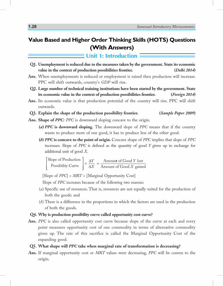
Q3. Explain the shape of the production possibility frontier. (Sample Paper 2009)
Ans. Shape of PPC: PPC is downward sloping concave to the origin.(a) PPC is downward sloping. The downward slope of PPC means that if the country
wants to produce more of one good, it has to produce less of the other good.(b) PPC is concave to the point of origin. Concave shape of PPC implies that slope of PPC
increases. Slope of PPC is defined as the quantity of good Y given up in exchange for additional unit of good X.
Slope of Production Possibility Curve Amoun
= =∆∆YX
tt of Good lostAmount of Good gained
YX
[Slope of PPC] = MRT = [Marginal Opportunity Cost] Slope of PPC increases because of the following two reasons:
(a) Specific use of resources. That is, resources are not equally suited for the production of both the goods: and
(b) There is a difference in the proportions in which the factors are used in the production of both the goods.
Q4. Why is production possibility curve called opportunity cost curve?
Ans. PPC is also called opportunity cost curve because slope of the curve at each and every point measures opportunity cost of one commodity in terms of alternative commodity given up. The rate of this sacrifice is called the Marginal Opportunity Cost of the expanding good.
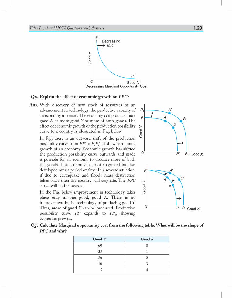
Q5. What shape will PPC take when marginal rate of transformation is decreasing?
Ans. If marginal opportunity cost or MRT values were decreasing, PPC will be convex to the origin.
Value Based and HOTS Questions with Answers 1.29
P
Goo
dY
P’
Good XO
DecreasingMRT
Decreasing Marginal Opportunity Cost
Q6. Explain the effect of economic growth on PPC?
Ans. With discovery of new stock of resources or an advancement in technology, the productive capacity of an economy increases. The economy can produce more good X or more good Y or more of both goods. The effect of economic growth onthe production possibility curve to a country is illustrated in Fig. below
In Fig. there is an outward shift of the production possibility curve from PP' to P1P1' . It shows economic growth of an economy. Economic growth has shifted the production possibility curve outwards and made it possible for an economy to produce more of both the goods. The economy has not stagnated but has developed over a period of time. In a reverse situation, if due to earthquake and floods mass destruction takes place then the country will stagnate. The PPC curve will shift inwards.
In the Fig. below improvement in technology takes place only in one good, good X. There is no improvement in the technology of producing good Y. Thus, more of good X can be produced. Production possibility curve PP' expands to PP1, showing economic growth.
Q7. Calculate Marginal opportunity cost from the following table. What will be the shape of PPC and why?
Good A Good B
60 035 120 210 35 4
Good X
B
B '
A '
A
Go
od
Y
P
O P1P '
Good X
B
A'
A
Good
Y
P1
P
P1'P'O
B'
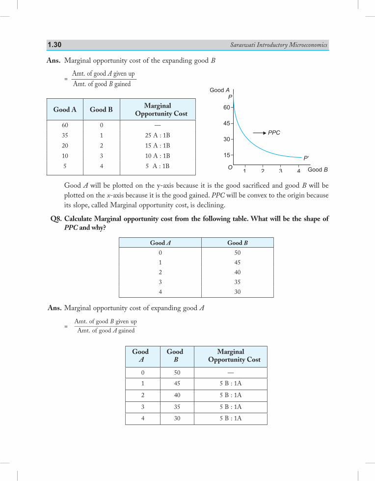
Saraswati Introductory Microeconomics1.30
Ans. Marginal opportunity cost of the expanding good B
= Amt. of good A given up
Amt. of good B gained
Good A Good B Marginal Opportunity Cost
60 0 —35 1 25 A : 1B20 2 15 A : 1B10 3 10 A : 1B5 4 5 A : 1B
Good A will be plotted on the y-axis because it is the good sacrificed and good B will be plotted on the x-axis because it is the good gained. PPC will be convex to the origin because its slope, called Marginal opportunity cost, is declining.
Q8. Calculate Marginal opportunity cost from the following table. What will be the shape of PPC and why?
Good A Good B
0 501 452 403 354 30
Ans. Marginal opportunity cost of expanding good A
= Amt. of good B given up
Amt. of good A gained
Good A
Good B
Marginal Opportunity Cost
0 50 —
1 45 5 B : 1A
2 40 5 B : 1A
3 35 5 B : 1A
4 30 5 B : 1A
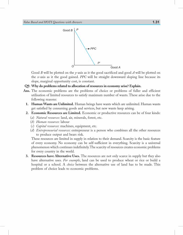
Value Based and HOTS Questions with Answers 1.31
Good AO
Good B P
P�
PPC
Good B will be plotted on the y-axis as it the good sacrificed and good A will be plotted on the x-axis as it the good gained. PPC will be straight downward sloping line because its slope, marginal opportunity cost, is constant.
Q9. Why do problems related to allocation of resources in economy arise? Explain. Ans. The economic problems are the problems of choice or problems of fuller and efficient
utilisation of limited resources to satisfy maximum number of wants. These arise due to the following reasons:
1. Human Wants are Unlimited. Human beings have wants which are unlimited. Human wants get satisfied by consuming goods and services, but new wants keep arising.
2. Economic Resources are Limited. Economic or productive resources can be of four kinds: (a) Natural resources: land, air, minerals, forest, etc. (b) Human resources: labour (c) Capital resources: machines, equipment, etc. (d) Entrepreneurial resources: entrepreneur is a person who combines all the other resources
to produce output and bears risk. These resources are limited in supply in relation to their demand. Scarcity is the basic feature
of every economy. No economy can be self-sufficient in everything. Scarcity is a universal phenomenon which continues indefinitely. The scarcity of resources creates economic problems for every country in the world.
3. Resources have Alternative Uses. The resources are not only scarce in supply but they also have alternative uses. For example, land can be used to produce wheat or rice or build a hospital or a school. A choice between the alternative use of land has to be made. This problem of choice leads to economic problems.
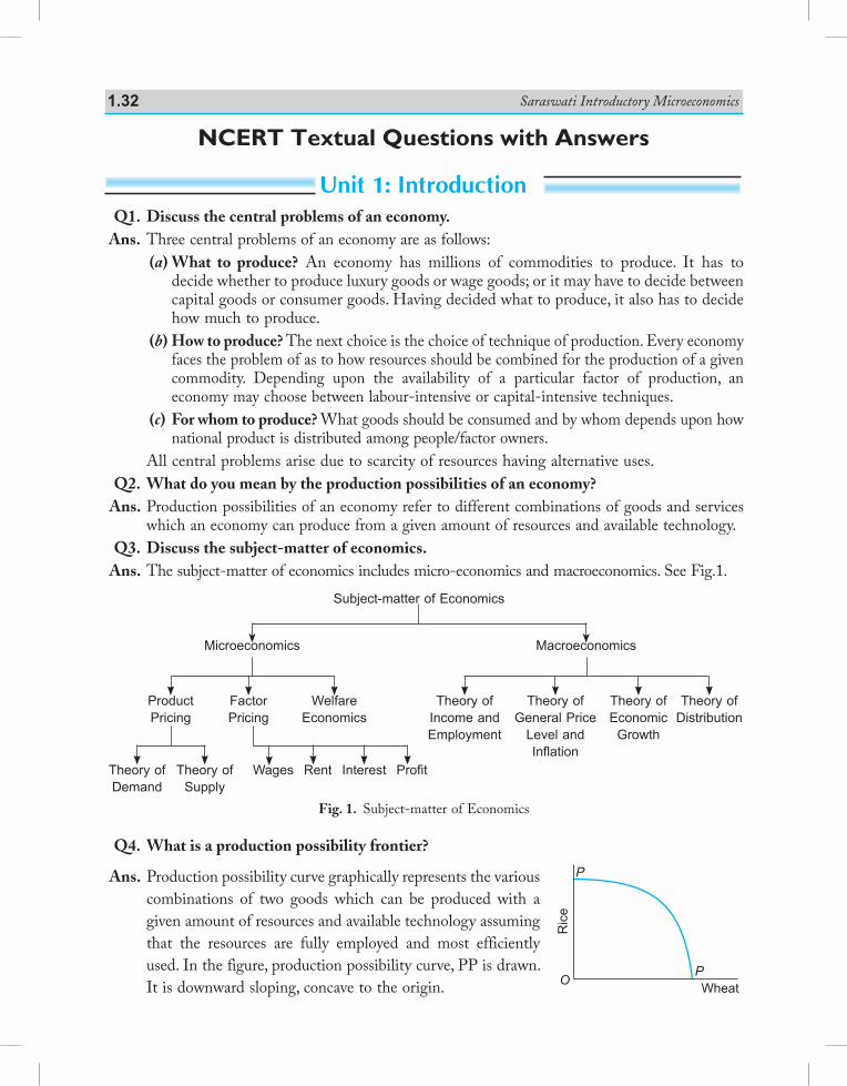
Saraswati Introductory Microeconomics1.32
Unit 1: Introduction
NCERT Textual Questions with Answers
Q1. Discuss the central problems of an economy. Ans. Three central problems of an economy are as follows:
(a) What to produce? An economy has millions of commodities to produce. It has to decide whether to produce luxury goods or wage goods; or it may have to decide between cap i tal goods or consumer goods. Having decided what to produce, it also has to decide how much to produce.
(b) How to produce? The next choice is the choice of technique of production. Every econ o my faces the problem of as to how resources should be combined for the production of a given commodity. Depending upon the availability of a particular factor of production, an economy may choose between labour-intensive or capital-intensive techniques.
(c) For whom to produce? What goods should be consumed and by whom depends upon how national product is distributed among people/factor owners.
All central problems arise due to scarcity of resources having alternative uses. Q2. What do you mean by the production possibilities of an economy? Ans. Production possibilities of an economy refer to different combinations of goods and services
which an economy can produce from a given amount of resources and available technology. Q3. Discuss the subject-matter of economics. Ans. The subject-matter of economics includes micro-economics and macroeconomics. See Fig.1.
Q4. What is a production possibility frontier?
Ans. Production possibility curve graphically represents the various combinations of two goods which can be produced with a given amount of resources and available technology assuming that the resources are fully employed and most efficiently used. In the figure, production possibility curve, PP is drawn. It is downward sloping, concave to the origin.
Fig. 1. Subject-matter of Economics
Subject-matter of Economics
Microeconomics
Wages Rent Interest Profit
Macroeconomics
ProductPricing
Theory ofGeneral Price
Level andInflation
Theory ofIncome andEmployment
Theory ofDemand
FactorPricing
Theory ofEconomic
Growth
Theory ofSupply
WelfareEconomics
Theory ofDistribution
P
P
Wheat
Ric
e
O
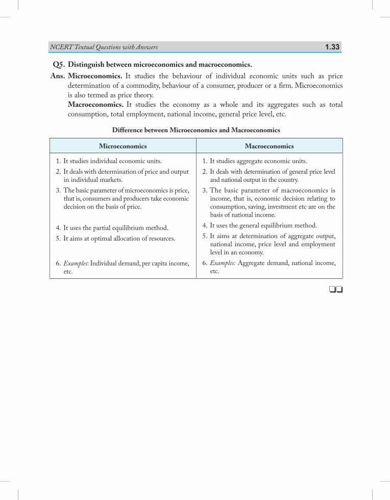
NCERT Textual Questions with Answers 1.33
Q5. Distinguish between microeconomics and macroeconomics. Ans. Microeconomics. It studies the behaviour of individual economic units such as price
determination of a commodity, behaviour of a consumer, producer or a firm. Microeconomics is also termed as price theory.
Macroeconomics. It studies the economy as a whole and its aggregates such as total consumption, total employment, national income, general price level, etc.
Difference between Microeconomics and Macroeconomics
Microeconomics Macroeconomics
1. It studies individual economic units.2. It deals with determination of price and output
in individual markets.3. The basic parameter of microeconomics is price,
that is, consumers and producers take economic decision on the basis of price.
4. It uses the partial equilibrium method.5. It aims at optimal allocation of resources.
6. Examples: Individual demand, per capita income, etc.
1. It studies aggregate economic units.2. It deals with determination of general price level
and national output in the country.3. The basic parameter of macroeconomics is
income, that is, economic decision relating to consumption, saving, investment etc are on the basis of national income.
4. It uses the general equilibrium method.5. It aims at determination of aggregate output,
national income, price level and employment level in an economy.
6. Examples: Aggregate demand, national income, etc.
oo


Consumer’s Equilibriumand
Demand
UNIT–2

This Unit Contains2. Consumer’s Equilibrium3. Demand4. Elasticity of Demand

2.1 IntroductIon to consumer’s equIlIbrIumA consumer is one who buys goods and services for satisfaction of wants. The objective of a consumer is to get maximum satisfaction from spending his income on various goods and services, given prices.Suppose a consumer wants to buy a commodity. How much of it should he buy? Two approaches are used for getting an answer to this question. These are:1. Utility approach2. Indifference curve approach2.2 consumer’s equIlIbrIum wIth utIlIty approach
2.2.1 Utility—Different Concepts1. Utility. Utility does not mean usefulness. The term utility refers to the want satisfying
power of a commodity. It means realised satisfaction to a consumer when he is willing to spend money on a stock of commodity which has the capacity to satisfy his want. Expected satisfaction is different from realised satisfaction. Realised satisfaction takes place only after the commodity has been consumed. Expected
2Consumer’s Equilibrium
2.1 Introduction to Consumer’s Equilibrium2.2 Consumer’s Equilibrium with Utility
Approach 2.2.1 Utility—Different Concepts 1. Utility 2. Total Utility 3. Marginal Utility 4. Relationship between TU and MU
Curves 2.2.2 The Law of Diminishing Marginal
Utility 2.2.3 Assumptions of the Utility Approach 2.2.4 Consumer’s Equilibrium: Meaning Case I: One Commodity Case Case II: Many Commodities Case—
Law of Equi-Marginal Utility
2.3 Consumer’s Equilibrium with Indifference Curve Approach
2.3.1 Assumptions of the Indifference Curve Approach
2.3.2 Indifference Curve 2.3.3 Indifference Schedule 2.3.4 Indifference Map 2.3.5 Properties or Features of Indifference
Curve 2.3.6 Budget Line or Income Line 2.3.7 Consumer’s Equilibrium or Optimal
Choice2.4 Comparison of Utility Approach with
Indifference Curve Approach Solved Numerical Problems Points to Remember Test Your Knowledge Answers to MCQs
Chapter Scheme
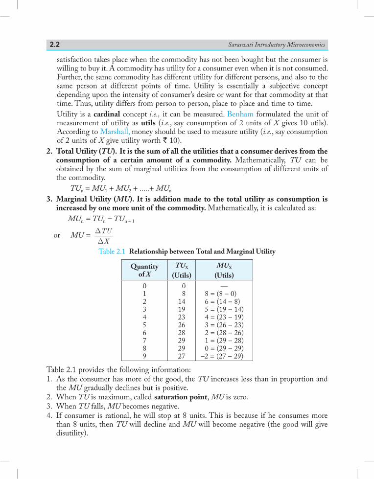
Saraswati Introductory Microeconomics2.2
satisfaction takes place when the commodity has not been bought but the consumer is willing to buy it. A commodity has utility for a consumer even when it is not consumed. Further, the same commodity has different utility for different persons, and also to the same person at different points of time. Utility is essentially a subjective concept depending upon the intensity of consumer’s desire or want for that commodity at that time. Thus, utility differs from person to person, place to place and time to time.
Utility is a cardinal concept i.e., it can be measured. Benham formulated the unit of measurement of utility as utils (i.e., say consumption of 2 units of X gives 10 utils). According to Marshall, money should be used to measure utility (i.e., say consumption of 2 units of X give utility worth ` 10).
2. Total Utility (TU). It is the sum of all the utilities that a consumer derives from the consumption of a certain amount of a commodity. Mathematically, TU can be obtained by the sum of marginal utilities from the consumption of different units of the commodity. TUn = MU1 + MU2 + .....+ MUn
3. Marginal Utility (MU). It is addition made to the total utility as consumption is increased by one more unit of the commodity. Mathematically, it is calculated as:
MUn = TUn – TUn – 1
or MU = DDTU
X
Table 2.1 Relationship between Total and Marginal Utility
Quantity of X
TUX
(Utils)MUX
(Utils)0123456789
0 81419232628292927
—8 = (8 – 0)6 = (14 – 8)5 = (19 – 14)4 = (23 – 19)3 = (26 – 23)2 = (28 – 26)1 = (29 – 28)0 = (29 – 29)
–2 = (27 – 29)
Table 2.1 provides the following information:1. As the consumer has more of the good, the TU increases less than in proportion and
the MU gradually declines but is positive.2. When TU is maximum, called saturation point, MU is zero.3. When TU falls, MU becomes negative.4. If consumer is rational, he will stop at 8 units. This is because if he consumes more
than 8 units, then TU will decline and MU will become negative (the good will give disutility).
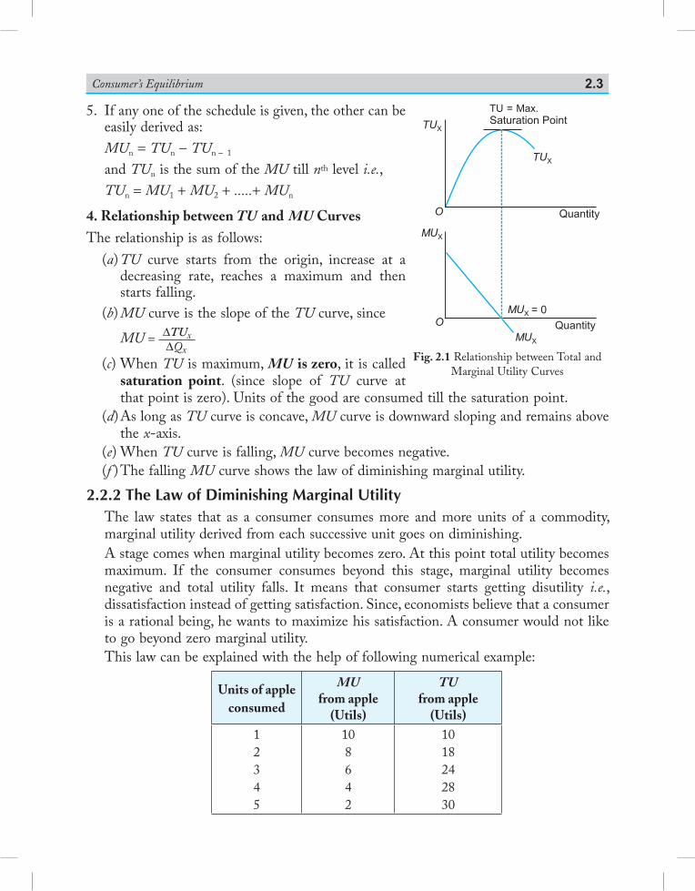
Consumer’s Equilibrium 2.3
5. If any one of the schedule is given, the other can be easily derived as:
MUn = TUn – TUn – 1 and TUn is the sum of the MU till nth level i.e., TUn = MU1 + MU2 + .....+ MUn
4. Relationship between TU and MU CurvesThe relationship is as follows: (a) TU curve starts from the origin, increase at a
decreasing rate, reaches a maximum and then starts falling.
(b) MU curve is the slope of the TU curve, since
MU = ∆TUX
∆QX
(c) When TU is maximum, MU is zero, it is called saturation point. (since slope of TU curve at that point is zero). Units of the good are consumed till the saturation point.
(d) As long as TU curve is concave, MU curve is downward sloping and remains above the x-axis.
(e) When TU curve is falling, MU curve becomes negative. (f ) The falling MU curve shows the law of diminishing marginal utility.2.2.2 The Law of Diminishing Marginal Utility The law states that as a consumer consumes more and more units of a commodity,
marginal utility derived from each successive unit goes on diminishing. A stage comes when marginal utility becomes zero. At this point total utility becomes
maximum. If the consumer consumes beyond this stage, marginal utility becomes negative and total utility falls. It means that consumer starts getting disutility i.e., dissatisfaction instead of getting satisfaction. Since, economists believe that a consumer is a rational being, he wants to maximize his satisfaction. A consumer would not like to go beyond zero marginal utility.
This law can be explained with the help of following numerical example:
Units of apple consumed
MUfrom apple
(Utils)
TUfrom apple
(Utils)12345
108642
1018242830
= 0
Quantity
Quantity
O
Saturation PointTU
X
O
TUX
MUX
MUX
MUX
Fig. 2.1 Relationship between Total and Marginal Utility Curves
TU = Max.
Saraswati Introductory Microeconomics2.4
The above table shows that as a consumer consumes first unit of apple, he gets 10 utils as marginal utility. When he consumes 2nd unit he gets 8 utils as marginal utility and so on. This proves that marginal utility declines continuously as the consumer consumes more and more units of the same commodity.
Assumptions of the Law of DMU. The law of DMU holds good when the following assumptions are satisfied:
1. Standard unit of measurement is used. If the unit of measurement is very large or very small then the law will not hold. Examples of inappropriate units are: rice measured in grammes, water in drops, diamonds in kilograms.
2. Homogeneous commodity. All units of the commodity consumed are homogeneous and perfect substitutes.
3. Continuous consumption. The law of DMU holds only when consumption of successive units of a commodity is without a time gap.
4. Mental and social condition of the consumer must be normal. The law will hold when consumer’s mental condition is normal. His income and tastes are unchanged and his behaviour is rational.
2.2.3 Assumptions of the Utility ApproachThe assumptions of the cardinal utility approach are:1. Utility can be measured, i.e. can be expressed in exact units. Utility is measurable in
monetary terms.2. Consumer’s income is given.3. Prices of commodities are given and remain constant. 4. Constant Marginal Utility of Money. It means that importance of money remains
unchanged. Marginal utility of money is addition made to utility of the consumer as he spends one more unit of the money income. This is assumed to be constant.
2.2.4 Consumer’s Equilibrium: MeaningA consumer is said to be in equilibrium when he maximizes his satisfaction, given income and prices of the commodities. In economics, consumer is the one who takes decisions about what to buy for satisfaction of wants. Consumer takes decision on the basis of his preferences, his income and the prices of the commodities which are prevailing in the market. Case I. One Commodity CaseLet us suppose that a consumer has a given income with which he consumes only one commodity X. Since both his money income and commodity X have utility for him, he can either spend his money income on commodity X or retain it with himself. If the consumer holds his income, the marginal utility of commodity (MUX) becomes greater
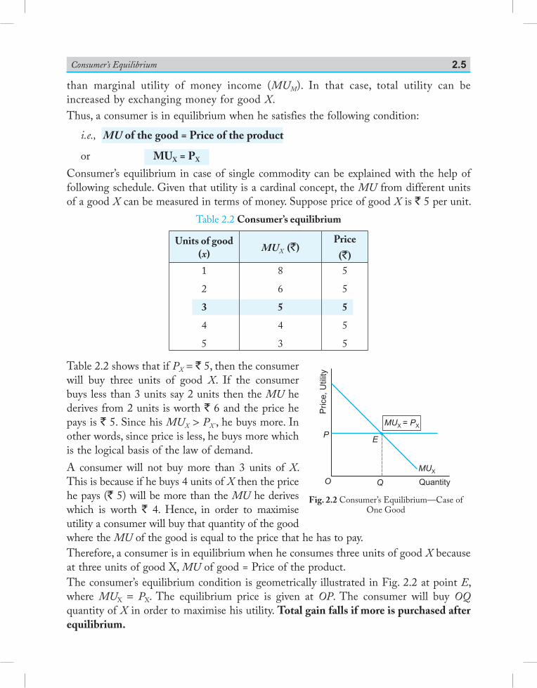
Consumer’s Equilibrium 2.5
than marginal utility of money income (MUM). In that case, total utility can be increased by exchanging money for good X. Thus, a consumer is in equilibrium when he satisfies the following condition:
i.e., MU of the good = Price of the product
or MUX = PX
Consumer’s equilibrium in case of single commodity can be explained with the help of following schedule. Given that utility is a cardinal concept, the MU from different units of a good X can be measured in terms of money. Suppose price of good X is ` 5 per unit.
Table 2.2 Consumer’s equilibrium
Units of good (x) MUX (`)
Price
(`)1
2
3
4
5
8
6
5
4
3
5
5
5
5
5
Table 2.2 shows that if PX = ` 5, then the consumer will buy three units of good X. If the consumer buys less than 3 units say 2 units then the MU he derives from 2 units is worth ` 6 and the price he pays is ` 5. Since his MUX > PX' , he buys more. In other words, since price is less, he buys more which is the logical basis of the law of demand.A consumer will not buy more than 3 units of X. This is because if he buys 4 units of X then the price he pays (` 5) will be more than the MU he derives which is worth ` 4. Hence, in order to maximise utility a consumer will buy that quantity of the good where the MU of the good is equal to the price that he has to pay. Therefore, a consumer is in equilibrium when he consumes three units of good X because at three units of good X, MU of good = Price of the product.The consumer’s equilibrium condition is geometrically illustrated in Fig. 2.2 at point E, where MUX = PX. The equilibrium price is given at OP. The consumer will buy OQ quantity of X in order to maximise his utility. Total gain falls if more is purchased after equilibrium.
Fig. 2.2 Consumer’s Equilibrium—Case of One Good
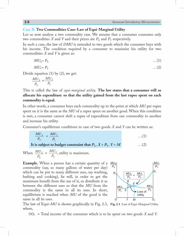
Saraswati Introductory Microeconomics2.6
Case II. Two Commodities Case–Law of Equi-Marginal UtilityLet us now analyse a two commodity case. We assume that a consumer consumes only two commodities X and Y and their prices are PX and PY respectively.In such a case, the law of DMU is extended to two goods which the consumer buys with his income. The condition required by a consumer to maximise his utility for two commodities X and Y is given as:
MUX = PX ... (1)
MUY = PY ... (2)Divide equation (1) by (2), we get:
MUP
X
X
= MUP
Y
Y
This is called the law of equi-marginal utility. The law states that a consumer will so allocate his expenditure so that the utility gained from the last rupee spent on each commodity is equal. In other words, a consumer buys each commodity up to the point at which MU per rupee spent on it is the same as the MU of a rupee spent on another good. When this condition is met, a consumer cannot shift a rupee of expenditure from one commodity to another and increase his utility.Consumer’s equilibrium conditions in case of two goods X and Y can be written as:
MUP
X
X
= MUP
Y
Y
…(1)
It is subject to budget constraint that PX . X + PY . Y = M …(2)
When MUP
X
X
= MUP
Y
Y
, utility is maximum.
Example. When a person has a certain quantity of a commodity (say, so many gallons of water per day) which can be put to many different uses, say washing, bathing and cooking), he will, in order to get the maximum benefit from the use of it, so distribute it as between the different uses so that the MU from the commodity is the same in all its uses. In short, equilibrium is reached when MU of the good is the same in all its uses.The law of Equi-MU is shown graphically in Fig. 2.3, where, OO1 = Total income of the consumer which is to be spent on two goods X and Y.
S1
O1MTO
R1
SLoss of
Utility
RE
MU
P
X
X
MU
P
Y
Y
MU
P
X
X
MU
P
Y
Y
MU
P
Y
Y
MU
P
X
X
Fig. 2.3 Law of Equi-Marginal Utility
Consumer’s Equilibrium 2.7
MUX = MU curve for good X as the successive rupees are spent on X.
Also, MUP
X
X
values can be obtained as PX is given and fixed.
MUY = MU curve for good Y as the successive rupees are spent on Y.
Also, MUP
Y
Y
values can be obtained as PY is given and fixed.
E = Point of consumer’s equilibrium where the law of Equi-marginal utility holds
i.e. MUP
X
X
= MUP
Y
Y
. It shows that OM amount of income is spent on good X
and O1M on good Y. The consumer’s total utility at point E = OR1ES1O1.
What happens when MUP
X
X
is not equal to MUP
Y
Y
? Two disequilibrium situations
are:
(1) MUX
PX >
MUY
PY : In this case, the consumer is getting more marginal utility per rupee in
case of good X as compared to Y. Therefore, he will buy more of X and less of Y. This will lead to fall in MUX and rise in MUY. The consumer will continue to buy more units of X till MU
PX
X
= MUP
Y
Y
.
(2) MUX
PX <
MUY
PY : The consumer is getting more marginal utility per rupee in case of
good Y as compared to X. Therefore, he will buy more of Y and less of X. This will lead fall in MUY and rise in MUX. The consumer
will continue to buy more of Y till MUP
X
X
= MUP
Y
Y
.
2.3 consumer’s equIlIbrIum wIth IndIfference curve approach
2.3.1 Assumptions of the Indifference Curve ApproachThe indifference curve approach is based on a few simple yet powerful assumptions. These assumptions are:1. Rationality. The consumer is assumed to be rational. He aims at maximising his
benefits from consumption, given his income and prices of the goods.2. Ordinality. Utility is expected satisfaction that a consumer gets from a given market
basket. In indifference curve analysis, utility is an ordinal concept. Consumer can order or rank the subjective utilities derived from the commodities.
Indifference means that a consumer considers one alternative exactly as good as the other.
Saraswati Introductory Microeconomics2.8
3. Diminishing Marginal Rate of Substitution. Scale of preferences are ranked in terms of indifference curves. Indifference curves are downward sloping convex-to-the origin curves. The slope of indifference curve is called Marginal Rate of Substitution (MRS) of X for Y. MRS is defined as the amount of good Y the consumer is willing to give up to consume an additional unit of good X, while leaving total utility unchanged. An important assumption is that the MRS of X for Y, decreases with greater quantities of good X, i.e. the greater the quantities of X, the less willing the consumer will be to give up Y in exchange for X. This relationship is known as the Law of Diminishing Marginal Rate of Substitution.
4. Consistency of Choice. Consumer is consistent in his choice. It means that if good X is preferred over good Y in one time period, then consumer will not prefer Y over X in another time period.
5. Transitivity of Choice. Consumer’s choices are characterised by the property of transitivity. If good X is preferred to good Y and good Y is preferred to good Z, then good X is preferred to good Z or x > z.
6. Monotonic Preference. A consumer’s preferences are monotonic if and only if between any two bundles, the consumer prefers the bundle which has more of at least one of the goods and no less of the other good as compared to the other bundle.
Example.
(a) A consumer with monotonic preference will prefer the bundle (2, 3) to bundles (2, 2), (1, 3) and (1, 2) bundles.
(b) A consumer with monotonic preference will prefer the bundle (2, 2) to (1, 1), (2, 1) and (1, 2) bundles.
Thus, monotonicity of preferences implies that (Fig 2.4) point M (which is above the indifference curve) represent a bundle which is preferred to the bundle on the indifference curve.2.3.2 Indifference Curve
An indifference curve shows different combinations of two goods that yield the same level of utility or satisfaction to the consumer. An indifference curve is downward sloping convex to the origin. Smoothness of the curve implies that the two goods X and Y are prefectly divisible into very small units.2.3.3 Indifference ScheduleIt is a tabular presentation of various combinations of two goods that yield the same level of satisfaction to the consumer.
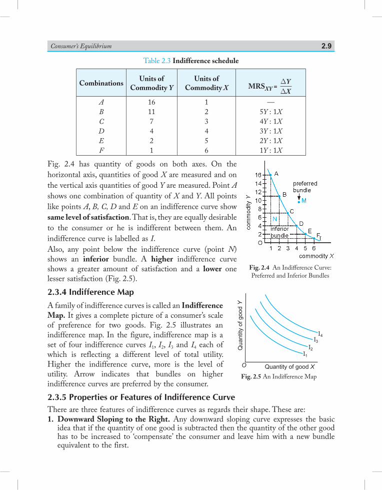
Consumer’s Equilibrium 2.9
Table 2.3 Indifference schedule
CombinationsUnits of
Commodity YUnits of
Commodity X MRSXY = DD
YX
ABCDEF
16117421
123456
—5Y : 1X4Y : 1X3Y : 1X2Y : 1X1Y : 1X
Fig. 2.4 has quantity of goods on both axes. On the horizontal axis, quantities of good X are measured and on the vertical axis quantities of good Y are measured. Point A shows one combination of quantity of X and Y. All points like points A, B, C, D and E on an indifference curve show same level of satisfaction. That is, they are equally desirable to the consumer or he is indifferent between them. An indifference curve is labelled as I.Also, any point below the indifference curve (point N) shows an inferior bundle. A higher indifference curve shows a greater amount of satisfaction and a lower one lesser satisfaction (Fig. 2.5).2.3.4 Indifference MapA family of indifference curves is called an Indifference Map. It gives a complete picture of a consumer’s scale of preference for two goods. Fig. 2.5 illustrates an indifference map. In the figure, indifference map is a set of four indifference curves I1, I2, I3 and I4 each of which is reflecting a different level of total utility. Higher the indifference curve, more is the level of utility. Arrow indicates that bundles on higher indifference curves are preferred by the consumer.2.3.5 Properties or Features of Indifference CurveThere are three features of indifference curves as regards their shape. These are:1. Downward Sloping to the Right. Any downward sloping curve expresses the basic
idea that if the quantity of one good is subtracted then the quantity of the other good has to be increased to ‘compensate’ the consumer and leave him with a new bundle equivalent to the first.
Fig. 2.4 An Indifference Curve: Preferred and Inferior Bundles
Fig. 2.5 An Indifference Map
Qua
ntity
of g
ood
Y
O Quantity of good X
I1
I2
I3
I4
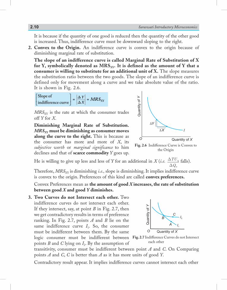
Saraswati Introductory Microeconomics2.10
It is because if the quantity of one good is reduced then the quantity of the other good is increased. Thus, indifference curve must be downward sloping to the right.
2. Convex to the Origin. An indifference curve is convex to the origin because of diminishing marginal rate of substitution.
The slope of an indifference curve is called Marginal Rate of Substitution of X for Y, symbolically denoted as MRSXY. It is defined as the amount of Y that a consumer is willing to substitute for an additional unit of X. The slope measures the substitution ratio between the two goods. The slope of an indifference curve is defined only for movement along a curve and we take absolute value of the ratio. It is shown in Fig. 2.6.
Slope of indifference curve
= D
DYX
= MRSXY
MRSXY is the rate at which the consumer trades off Y for X.
Diminishing Marginal Rate of Substitution. MRSXY must be diminishing as consumer moves along the curve to the right. This is because as the consumer has more and more of X, its subjective worth or marginal significance to him declines and that of scarce commodity Y goes up.
He is willing to give up less and less of Y for an additional in X (i.e. DD
TU
QX
X
falls).
Therefore, MRSXY is diminishing i.e., slope is diminishing. It implies indifference curve is convex to the origin. Preferences of this kind are called convex preferences.
Convex Preferences mean as the amount of good X increases, the rate of substitution between good X and good Y diminishes.
3. Two Curves do not Intersect each other. Two indifference curves do not intersect each other. If they intersect, say, at point B in Fig. 2.7, then we get contradictory results in terms of preference ranking. In Fig. 2.7, points A and B lie on the same indifference curve I1. So, the consumer must be indifferent between them. By the same logic consumer must be indifferent between points B and C lying on I2. By the assumption of transitivity, consumer must be indifferent between point A and C. On Comparing points A and C, C is better than A as it has more units of good Y.
Contradictory result appear. It implies indifference curves cannot intersect each other
Fig. 2.6 Indifference Curve is Convex to the Origin
Quantity of XQ
uan
tity
ofY
IX
Y
O
O
Quantity
ofY
Quantity of X
A
B
I1
I2
C
Fig. 2.7 Indifference Curves do not Intersect each other
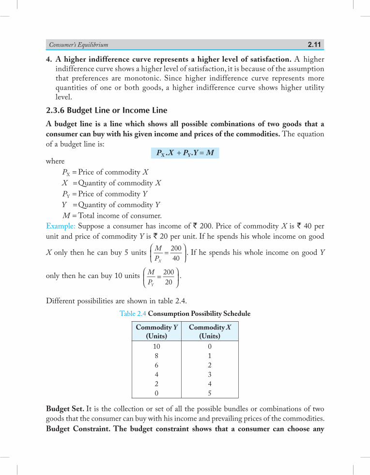
Consumer’s Equilibrium 2.11
4. A higher indifference curve represents a higher level of satisfaction. A higher indifference curve shows a higher level of satisfaction, it is because of the assumption that preferences are monotonic. Since higher indifference curve represents more quantities of one or both goods, a higher indifference curve shows higher utility level.
2.3.6 Budget Line or Income Line
A budget line is a line which shows all possible combinations of two goods that a consumer can buy with his given income and prices of the commodities. The equation of a budget line is:
PX .X + PY.Y = Mwhere PX = Price of commodity X
X = Quantity of commodity X PY = Price of commodity Y
Y = Quantity of commodity Y M = Total income of consumer.
Example: Suppose a consumer has income of ` 200. Price of commodity X is ` 40 per unit and price of commodity Y is ` 20 per unit. If he spends his whole income on good
X only then he can buy 5 units MPX
=
20040
. If he spends his whole income on good Y
only then he can buy 10 units MPY
=
20020
.
Different possibilities are shown in table 2.4.Table 2.4 Consumption Possibility Schedule
Commodity Y(Units)
Commodity X(Units)
1086420
012345
Budget Set. It is the collection or set of all the possible bundles or combinations of two goods that the consumer can buy with his income and prevailing prices of the commodities.Budget Constraint. The budget constraint shows that a consumer can choose any
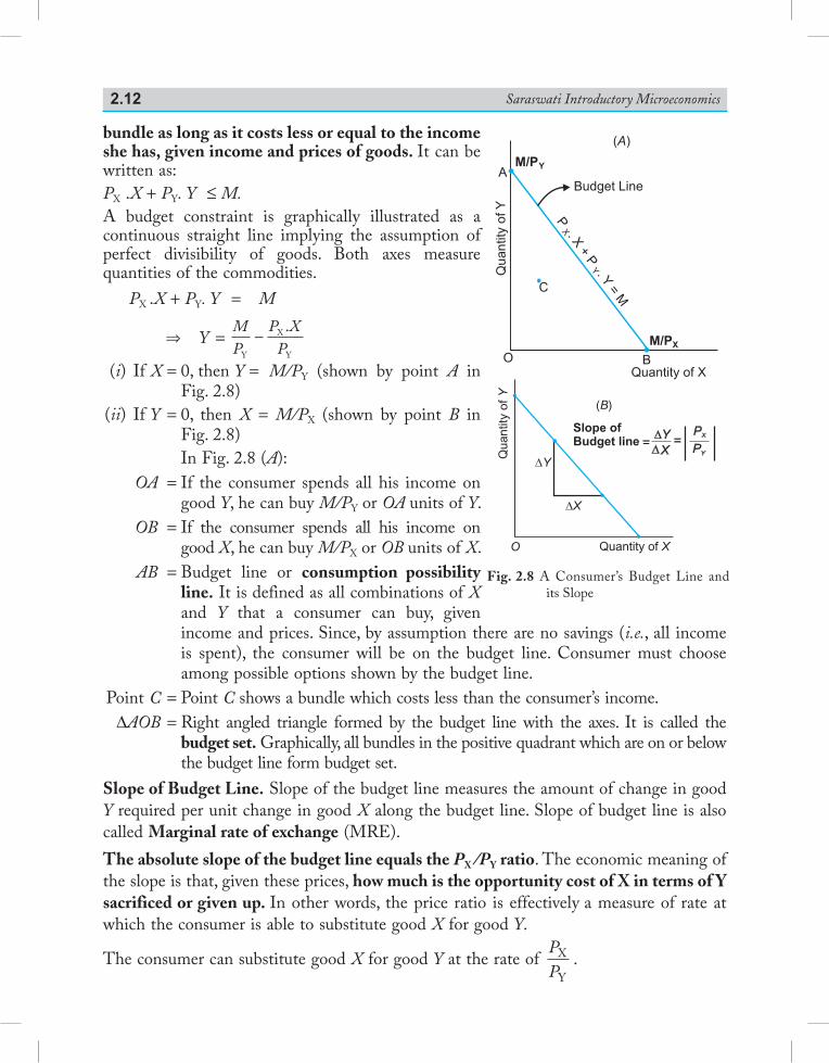
Saraswati Introductory Microeconomics2.12
bundle as long as it costs less or equal to the income she has, given income and prices of goods. It can be written as: PX .X + PY. Y ≤ M.A budget constraint is graphically illustrated as a continuous straight line implying the assumption of perfect divisibility of goods. Both axes measure quantities of the commodities.
PX .X + PY. Y = M
⇒ Y = MP
P XPY
X
Y
.−
(i) If X = 0, then Y = M/PY (shown by point A in Fig. 2.8)
(ii) If Y = 0, then X = M/PX (shown by point B in Fig. 2.8)
In Fig. 2.8 (A): OA = If the consumer spends all his income on
good Y, he can buy M/PY or OA units of Y. OB = If the consumer spends all his income on
good X, he can buy M/PX or OB units of X. AB = Budget line or consumption possibility
line. It is defined as all combinations of X and Y that a consumer can buy, given income and prices. Since, by assumption there are no savings (i.e., all income is spent), the consumer will be on the budget line. Consumer must choose among possible options shown by the budget line.
Point C = Point C shows a bundle which costs less than the consumer’s income. ΔAOB = Right angled triangle formed by the budget line with the axes. It is called the
budget set. Graphically, all bundles in the positive quadrant which are on or below the budget line form budget set.
Slope of Budget Line. Slope of the budget line measures the amount of change in good Y required per unit change in good X along the budget line. Slope of budget line is also called Marginal rate of exchange (MRE).The absolute slope of the budget line equals the PX /PY ratio. The economic meaning of the slope is that, given these prices, how much is the opportunity cost of X in terms of Y sacrificed or given up. In other words, the price ratio is effectively a measure of rate at which the consumer is able to substitute good X for good Y.
The consumer can substitute good X for good Y at the rate of PP
X
Y.
Fig. 2.8 A Consumer’s Budget Line and its Slope
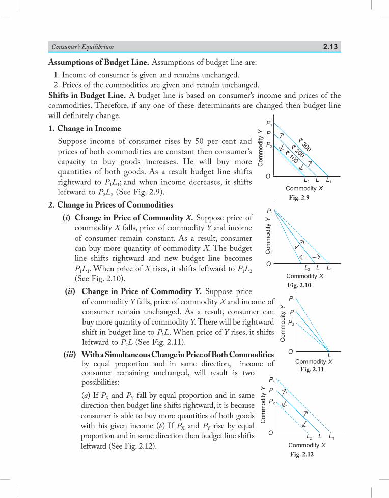
Consumer’s Equilibrium 2.13
Assumptions of Budget Line. Assumptions of budget line are: 1. Income of consumer is given and remains unchanged. 2. Prices of the commodities are given and remain unchanged.Shifts in Budget Line. A budget line is based on consumer’s income and prices of the commodities. Therefore, if any one of these determinants are changed then budget line will definitely change.1. Change in Income
Suppose income of consumer rises by 50 per cent and prices of both commodities are constant then consumer’s capacity to buy goods increases. He will buy more quantities of both goods. As a result budget line shifts rightward to P1L1; and when income decreases, it shifts leftward to P2L2 (See Fig. 2.9).
2. Change in Prices of Commodities
(i) Change in Price of Commodity X. Suppose price of commodity X falls, price of commodity Y and income of consumer remain constant. As a result, consumer can buy more quantity of commodity X. The budget line shifts rightward and new budget line becomes P1L1. When price of X rises, it shifts leftward to P1L2 (See Fig. 2.10).
(ii) Change in Price of Commodity Y. Suppose price of commodity Y falls, price of commodity X and income of consumer remain unchanged. As a result, consumer can buy more quantity of commodity Y. There will be rightward shift in budget line to P1L. When price of Y rises, it shifts leftward to P2L (See Fig. 2.11).
(iii) With a Simultaneous Change in Price of Both Commodities by equal proportion and in same direction, income of consumer remaining unchanged, will result is two possibilities:
(a) If PX and PY fall by equal proportion and in same direction then budget line shifts rightward, it is because consumer is able to buy more quantities of both goods with his given income (b) If PX and PY rise by equal proportion and in same direction then budget line shifts leftward (See Fig. 2.12).
L2
P2
P
P1
LCommodity X
` 100
` 200
` 300
Com
mod
ity Y
L1O
Fig. 2.9
Fig. 2.10
L2
P1
LCommodity X
Com
mod
ity Y
L1O
Fig. 2.11
P1
PP2
LCommodity X
Com
mod
ity Y
O
L2
P2
P
P1
LCommodity X
Com
mod
ity Y
L1O
Fig. 2.12
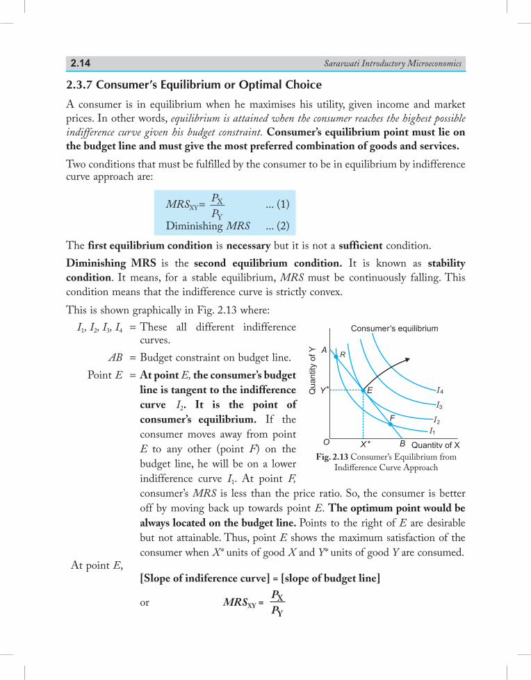
Saraswati Introductory Microeconomics2.14
2.3.7 Consumer’s Equilibrium or Optimal Choice
A consumer is in equilibrium when he maximises his utility, given income and market prices. In other words, equilibrium is attained when the consumer reaches the highest possible indifference curve given his budget constraint. Consumer’s equilibrium point must lie on the budget line and must give the most preferred combination of goods and services.
Two conditions that must be fulfilled by the consumer to be in equilibrium by indifference curve approach are:
MRSXY = PP
X
Y
... (1)
Diminishing MRS ... (2)
The first equilibrium condition is necessary but it is not a sufficient condition. Diminishing MRS is the second equilibrium condition. It is known as stability condition. It means, for a stable equilibrium, MRS must be continuously falling. This condition means that the indifference curve is strictly convex. This is shown graphically in Fig. 2.13 where: I1, I2, I3, I4 = These all different indifference
curves. AB = Budget constraint on budget line. Point E = At point E, the consumer’s budget
line is tangent to the indifference curve I2. It is the point of consumer’s equilibrium. If the consumer moves away from point E to any other (point F) on the budget line, he will be on a lower indifference curve I1. At point F, consumer’s MRS is less than the price ratio. So, the consumer is better off by moving back up towards point E. The optimum point would be always located on the budget line. Points to the right of E are desirable but not attainable. Thus, point E shows the maximum satisfaction of the consumer when X* units of good X and Y* units of good Y are consumed.
At point E, [Slope of indiference curve] = [slope of budget line]
or MRSXY = PP
X
Y
'
R
Fig. 2.13 Consumer’s Equilibrium from Indifference Curve Approach
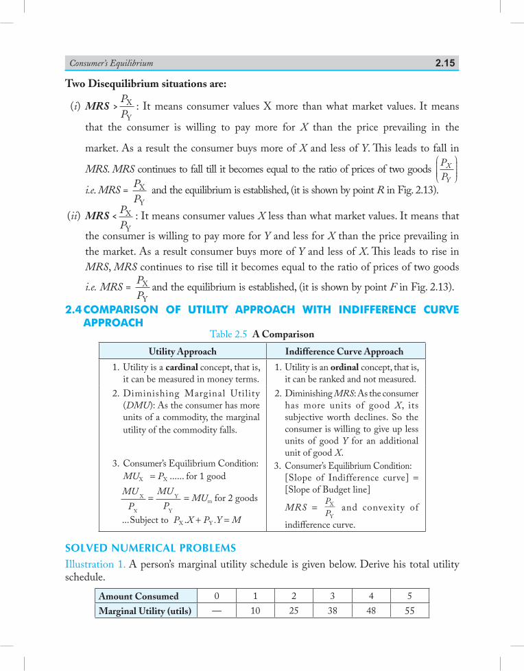
Consumer’s Equilibrium 2.15
Two Disequilibrium situations are:
(i) MRS >PP
X
Y: It means consumer values X more than what market values. It means
that the consumer is willing to pay more for X than the price prevailing in the
market. As a result the consumer buys more of X and less of Y. This leads to fall in
MRS. MRS continues to fall till it becomes equal to the ratio of prices of two goods PP
X
Y
i.e. MRS = PP
X
Y
and the equilibrium is established, (it is shown by point R in Fig. 2.13).
(ii) MRS < PP
X
Y
: It means consumer values X less than what market values. It means that
the consumer is willing to pay more for Y and less for X than the price prevailing in the market. As a result consumer buys more of Y and less of X. This leads to rise in MRS, MRS continues to rise till it becomes equal to the ratio of prices of two goods
i.e. MRS = PP
X
Yand the equilibrium is established, (it is shown by point F in Fig. 2.13).
2.4 comparIson of utIlIty approach wIth IndIfference curve approach
Table 2.5 A Comparison
Utility Approach Indifference Curve Approach
1. Utility is a cardinal concept, that is, it can be measured in money terms.
1. Utility is an ordinal concept, that is, it can be ranked and not measured.
2. Diminishing Marginal Utility (DMU): As the consumer has more units of a commodity, the marginal utility of the commodity falls.
3. Consumer’s Equilibrium Condition: MUX = PX ...... for 1 good
MU
PX
X
= MU
PY
Y
= MUm for 2 goods
... Subject to PX .X + PY .Y = M
2. Diminishing MRS: As the consumer has more units of good X, its subjective worth declines. So the consumer is willing to give up less units of good Y for an additional unit of good X.
3. Consumer’s Equilibrium Condition: [Slope of Indifference curve] =
[Slope of Budget line]
MRS = PP
X
Y and convexity of
indifference curve.
SOLVED NUMERICAL PROBLEMSIllustration 1. A person’s marginal utility schedule is given below. Derive his total utility schedule.
Amount Consumed 0 1 2 3 4 5Marginal Utility (utils) — 10 25 38 48 55
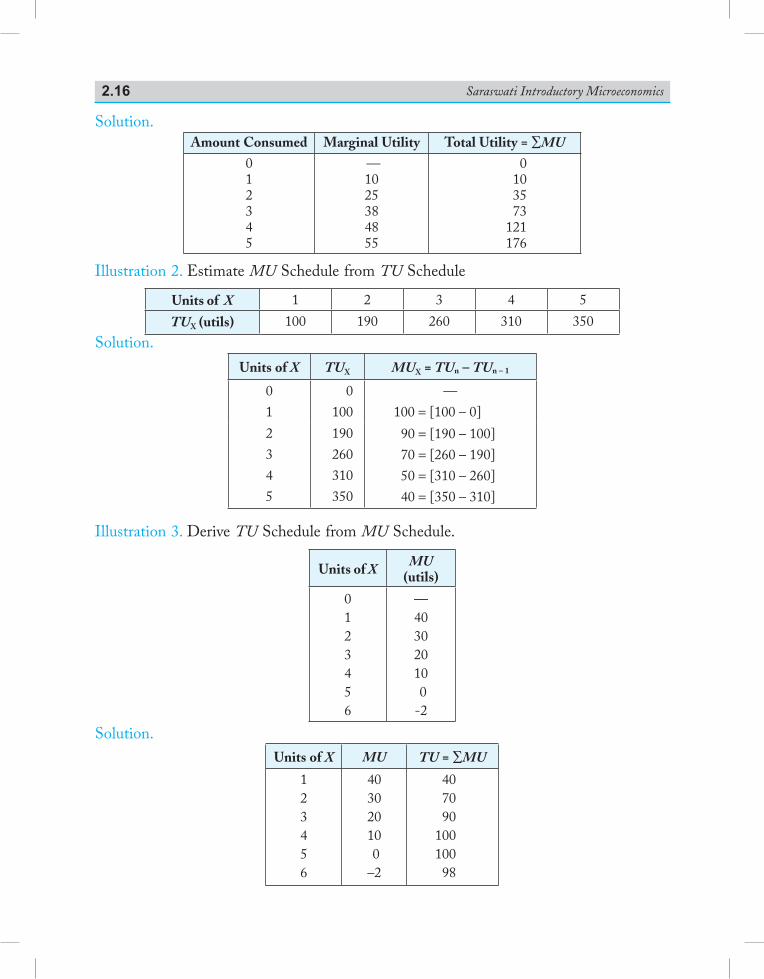
Saraswati Introductory Microeconomics2.16
Solution.Amount Consumed Marginal Utility Total Utility = ∑MU
012345
—1025384855
0103573
121176
Illustration 2. Estimate MU Schedule from TU Schedule
Units of X 1 2 3 4 5TUX (utils) 100 190 260 310 350
Solution.Units of X TUX MUX = TUn – TUn – 1
01
0100
—100 = [100 – 0]
2345
190260310350
90 = [190 – 100] 70 = [260 – 190] 50 = [310 – 260] 40 = [350 – 310]
Illustration 3. Derive TU Schedule from MU Schedule.
Units of X MU (utils)
0123456
—40302010 0-2
Solution.Units of X MU TU = ∑MU
123456
40302010 0–2
407090
10010098
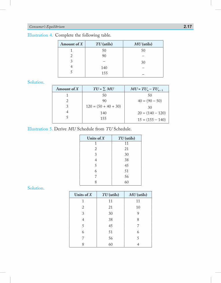
Consumer’s Equilibrium 2.17
Illustration 4. Complete the following table.
Amount of X TU (utils) MU (utils)
12345
5090–
140 155
50–30––
Solution.Amount of X TU = ∑ MU MU = TUn – TUn – 1
12345
5090
120 = (50 + 40 + 30)140155
5040 = (90 – 50)
30 20 = (140 – 120) 15 = (155 – 140)
Illustration 5. Derive MU Schedule from TU Schedule.
Units of X TU (utils)1 112 213 304 385 456 517 568 60
Solution.Units of X TU (utils) MU (utils)
1 11 112 21 103 30 94 38 85 45 76 51 67 56 58 60 4
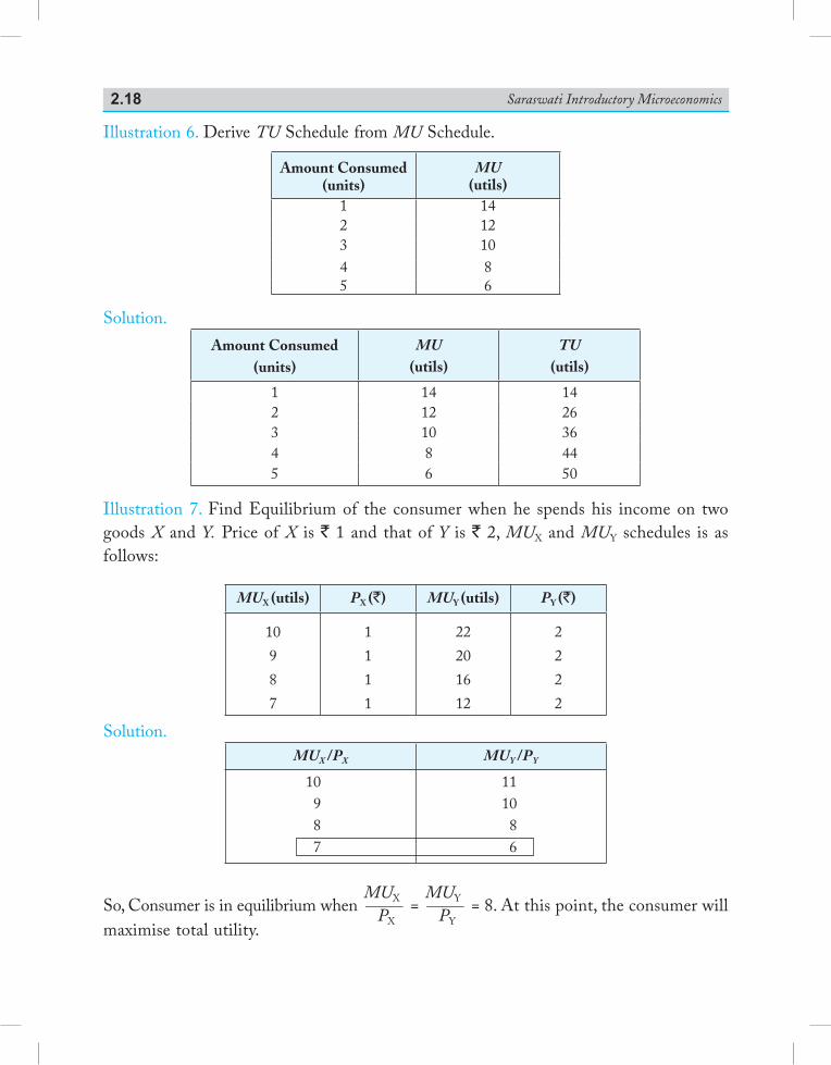
Saraswati Introductory Microeconomics2.18
Illustration 6. Derive TU Schedule from MU Schedule.
Amount Consumed(units)
MU(utils)
1 142 123 104 85 6
Solution.Amount Consumed
(units)MU
(utils)TU
(utils)
1 14 142 12 263 10 364 8 445 6 50
Illustration 7. Find Equilibrium of the consumer when he spends his income on two goods X and Y. Price of X is ` 1 and that of Y is ` 2, MUX and MUY schedules is as follows:
MUX (utils) PX (`) MUY (utils) PY (`)
10987
1111
22201612
2222
Solution. MUX /PX MUY /PY
10987
111086
So, Consumer is in equilibrium when MUX _____ PX
= MUY _____ PY
= 8. At this point, the consumer will maximise total utility.
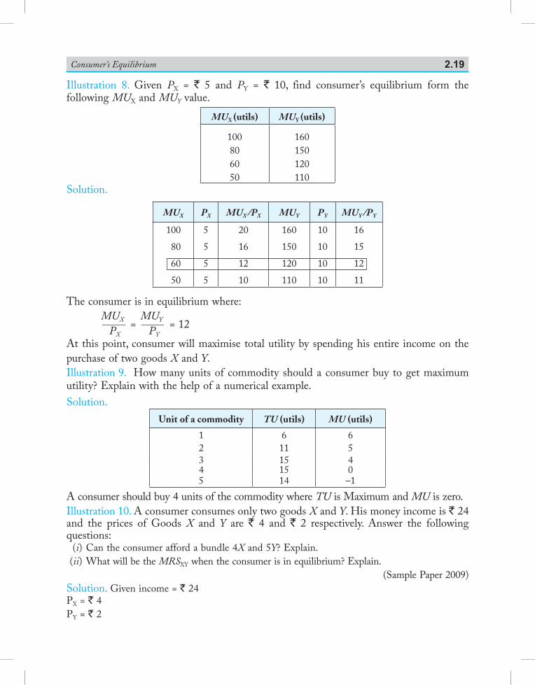
Consumer’s Equilibrium 2.19
Illustration 8. Given PX = ` 5 and PY = ` 10, find consumer’s equilibrium form the following MUX and MUY value.
MUX (utils) MUY (utils)
100806050
160150120110
Solution.
MUX PX MUX /PX MUY PY MUY /PY
100806050
5555
20161210
160150120110
10101010
16151211
The consumer is in equilibrium where:
MUX _____ PX
= MUY _____ PY
= 12
At this point, consumer will maximise total utility by spending his entire income on the purchase of two goods X and Y.Illustration 9. How many units of commodity should a consumer buy to get maximum utility? Explain with the help of a numerical example.Solution.
Unit of a commodity TU (utils) MU (utils)
1 6 62 11 53 15 44 15 05 14 –1
A consumer should buy 4 units of the commodity where TU is Maximum and MU is zero.Illustration 10. A consumer consumes only two goods X and Y. His money income is ` 24 and the prices of Goods X and Y are ` 4 and ` 2 respectively. Answer the following questions: (i) Can the consumer afford a bundle 4X and 5Y? Explain. (ii) What will be the MRSXY when the consumer is in equilibrium? Explain. (Sample Paper 2009)Solution. Given income = ` 24 PX = ` 4 PY = ` 2
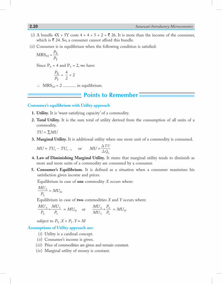
Saraswati Introductory Microeconomics2.20
(i) A bundle 4X + 5Y costs 4 × 4 + 5 × 2 = ` 26. It is more than the income of the consumer, which is ` 24. So, a consumer cannot afford this bundle.
(ii) Consumer is in equilibrium when the following condition is satisfied:
MRS XY =PP
X
Y× 4
2
Since PX = 4 and PY = 2, we have:
PP
X
Y× 4
2 = P
PX
Y× 4
2 = 2
∴ MRS XY = 2 ............ in equilibrium.
Points to RememberConsumer’s equilibrium with Utility approach
1. Utility. It is ‘want-satisfying capacity’ of a commodity. 2. Total Utility. It is the sum total of utility derived from the consumption of all units of a
commodity. TU = ∑MU
3. Marginal Utility. It is additional utility when one more unit of a commodity is consumed.
MU = TUn – TUn – 1 or MU = DDTUQ
X
4. Law of Diminishing Marginal Utility. It states that marginal utility tends to diminish as more and more units of a commodity are consumed by a consumer.
5. Consumer’s Equilibrium. It is defined as a situation when a consumer maximises his satisfaction given income and prices.
Equilibrium in case of one commodity X occurs where:
MUP
X
X
= MUM
Equilibrium in case of two commodities X and Y occurs where:
MU
PMU
PX
X
Y
Y
= = MUM or MUMU
PP
X
Y
X
Y
= = MUM
subject to PX .X + PY .Y = M
Assumptions of Utility approach are: (i) Utility is a cardinal concept. (ii) Consumer’s income is given. (iii) Price of commodities are given and remain constant. (iv) Marginal utility of money is constant.
Consumer’s Equilibrium 2.21
Indifference curve approach
1. It shows different combinations of goods that yield the same level of satisfaction to the consumer. A family of indifference curves is called an indifference map.
2. Features of indifference curve are: (i) Downwards sloping to the right, (ii) Convex to the origin. 3. Slope of an indifference curve is called Marginal Rate of Substitution (MRSXY). Assumptions of the Indifference curve approach (i) Rationality (ii) Ordinality (iii) Diminishing marginal rate of substitution (iv) Consistency or transitivity of choice (v) Monotonic preferenceBudget line
1. It shows all the possible combinations of the two goods that can be bought by a con sum er given income and prices of goods.
2. Slope of the budget line (MRE) is the price ratio, i.e., PP
X
Y
. 3. Budget line shifts if (i) price of any one or both goods changes, and (ii) money income
changes.Properties of Indifference curve approach
(i) Downward sloping to the Right. (ii) Convex to the Origin. (iii) Do not Intersect each other. (iv) A higher IC shows a higher level of satisfaction.Consumer’s equilibrium or optimal choice
1. A consumer is in equilibrium when he maximises his utility, given income and prices. 2. Equilibrium is reached at the point at tangency between indifference curve and budg et line.
Consumer equilibrium conditions are:
MRSXY = PP
X
Y
and Diminishing MRS.
Test Your KnowledgeVery Short Answer Type Questions (1 Mark)
1. Define utility. (Foreign 2014) 2. Define total utility.
Saraswati Introductory Microeconomics2.22
3. Define Marginal utility. (AI 2002, Foreign 2010) 4. Define diminishing marginal utility. 5. Define marginal rate of substitution 6. Define an indifference curve. (Delhi 2010; AI 2014) 7. Define budget set. (Delhi 2011, 14) 8. Define budget line. (AI 2010, 2011; Foreign 2013, Delhi 2014) 9. Define consumer’s optimum/equilibrium. (Foreign 2006, 13) 10. Give consumer’s optimum condition from utility approach in case of one good. 11. Give consumer’s optimum condition from indifference curve approach. 12. Define slope of TU curve. 13. Define slope of budget line. 14. Define slope of indifference curve. 15. Define saturation point. 16. State the law of equi-marginal utility. 17. What does an indifference curve show? (Foreign 2012) 18. Define indifference map. (Delhi 2014) 19. What is meant by monotonic preferences? (AI 2014) 20. What is law of diminishing marginal utility? (Foreign 2014) 21. Give equation of Budget Line. (Delhi 2015) 22. Define utility. (Foreign 2015) 23. When does ‘decrease’ in demand take place? (Foreign 2016) 24. Define indifference curve. (AI 2017)
Multiple Choice Questions
1. In Marginal utility theory, marginal utility of money: (a) Rises (b) Constant (c) Falls (d) Rises and then falls
2. In Marginal utility theory, utility is: (a) An ordinal concept (b) A cardinal concept (c) Both ordinal and cardinal concept (d) None of the above 3. As the consumer has more units of a commodity, his total utility from the commodity: (a) Increases less than in proportion, reaches a maximum and then falls (b) Increases less than in proportion and then falls (c) Increases more than in proportion and then reaches a maximum (d) Falls, becomes zero and then negative 4. MU of the commodity when no commodity is consumed is: (a) Maximum (b) Falling (c) Constant (d) Rising
Consumer’s Equilibrium 2.23
5. MU of the commodity becomes negative when TU of the commodity is: (a) Rising (b) Constant (c) Falling (d) Zero 6. When MU of the commodity is zero, slope of TU curve is: (a) Zero (b) Rising (c) Falling (d) Constant 7. Slope of TU curve is called: (a) Marginal utility (b) Utility (c) Average utility (d) None of the above 8. Saturation point means: (a) TU is rising, and MU is falling (b) TU is falling and MU is negative (c) TU is maximum and MU is zero (d) Falling MU curve 9. Falling MU curve shows which law? (a) Law of diminishing returns (b) Law of diminishing marginal rate of substitution (c) Law of diminishing marginal utility (d) None of the above 10. When MU is falling, TU is: (a) Rising (b) Falling (c) Not changing (d) Maximum 11. MRS is defined as: (a) Amount of good Y given up in exchange for good X such that total utility is constant (b) Amount of good X given up in exchange for good Y such that total utility is constant (c) Amount of good Y given up in exchange for good X such that total utility rises (d) Amount of good Y given up in exchange for good X 12. Indifference mean: (a) X is preferred to Y (b) Y is preferred to X (c) X and Y are equally preferred (d) None of the above 13. MRS is given by
(a) DDXY
(b) ΔX – ΔY
(c) DDYX
(d) ΔY – ΔX
14. Diminishing MRS means: (a) Consumer wants to give up lesser units of Y in exchange for good X (b) Consumer wants to give up more units of Y in exchange for good X (c) Consumer wants to give up same units of Y in exchange for good X (d) None of the above
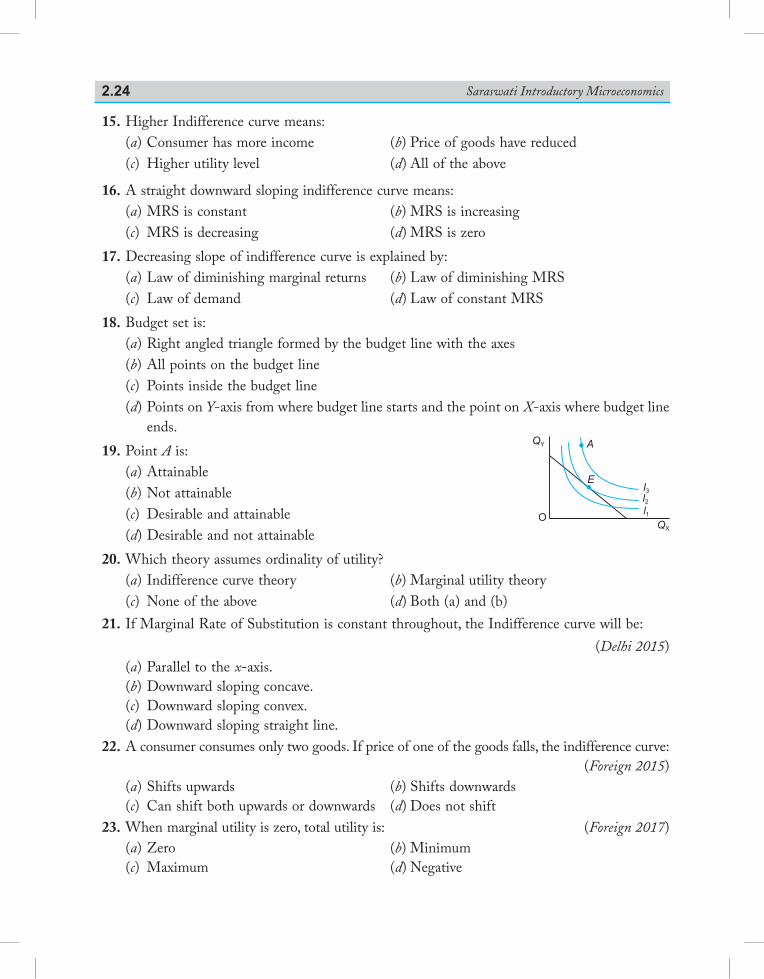
Saraswati Introductory Microeconomics2.24
15. Higher Indifference curve means: (a) Consumer has more income (b) Price of goods have reduced (c) Higher utility level (d) All of the above
16. A straight downward sloping indifference curve means: (a) MRS is constant (b) MRS is increasing (c) MRS is decreasing (d) MRS is zero 17. Decreasing slope of indifference curve is explained by: (a) Law of diminishing marginal returns (b) Law of diminishing MRS (c) Law of demand (d) Law of constant MRS 18. Budget set is: (a) Right angled triangle formed by the budget line with the axes (b) All points on the budget line (c) Points inside the budget line (d) Points on Y-axis from where budget line starts and the point on X-axis where budget line
ends. 19. Point A is: (a) Attainable (b) Not attainable (c) Desirable and attainable (d) Desirable and not attainable 20. Which theory assumes ordinality of utility? (a) Indifference curve theory (b) Marginal utility theory (c) None of the above (d) Both (a) and (b) 21. If Marginal Rate of Substitution is constant throughout, the Indifference curve will be: (Delhi 2015) (a) Parallel to the x-axis. (b) Downward sloping concave. (c) Downward sloping convex. (d) Downward sloping straight line. 22. A consumer consumes only two goods. If price of one of the goods falls, the indifference curve:
(Foreign 2015) (a) Shifts upwards (b) Shifts downwards (c) Can shift both upwards or downwards (d) Does not shift 23. When marginal utility is zero, total utility is: (Foreign 2017) (a) Zero (b) Minimum (c) Maximum (d) Negative
O
E
A
l1l2l3
QX
QY
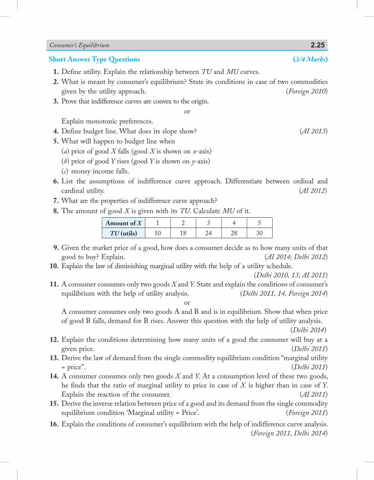
Consumer’s Equilibrium 2.25
Short Answer Type Questions (3/4 Marks)
1. Define utility. Explain the relationship between TU and MU curves. 2. What is meant by consumer’s equilibrium? State its conditions in case of two commodities
given by the utility approach. (Foreign 2010) 3. Prove that indifference curves are convex to the origin.
or Explain monotonic preferences. 4. Define budget line. What does its slope show? (AI 2013) 5. What will happen to budget line when
(a) price of good X falls (good X is shown on x-axis)(b) price of good Y rises (good Y is shown on y-axis)(c) money income falls.
6. List the assumptions of indifference curve approach. Differentiate between ordinal and cardinal utility. (AI 2012)
7. What are the properties of indifference curve approach? 8. The amount of good X is given with its TU. Calculate MU of it.
Amount of X 1 2 3 4 5TU (utils) 10 18 24 28 30
9. Given the market price of a good, how does a consumer decide as to how many units of that good to buy? Explain. (AI 2014; Delhi 2012)
10. Explain the law of diminishing marginal utility with the help of a utility schedule. (Delhi 2010, 13; AI 2011) 11. A consumer consumes only two goods X and Y. State and explain the conditions of consumer’s
equilibrium with the help of utility analysis. (Delhi 2011, 14, Foreign 2014)or
A consumer consumes only two goods A and B and is in equilibrium. Show that when price of good B falls, demand for B rises. Answer this question with the help of utility analysis. (Delhi 2014)
12. Explain the conditions determining how many units of a good the consumer will buy at a given price. (Delhi 2011)
13. Derive the law of demand from the single commodity equilibrium condition “marginal utility = price”. (Delhi 2011)
14. A consumer consumes only two goods X and Y. At a consumption level of these two goods, he finds that the ratio of marginal utility to price in case of is higher than in case of Y. Explain the reaction of the consumer. (AI 2011)
15. Derive the inverse relation between price of a good and its demand from the single commodity equilibrium condition ‘Marginal utility = Price’. (Foreign 2011)
16. Explain the conditions of consumer’s equilibrium with the help of indifference curve analysis.(Foreign 2011, Delhi 2014)
Saraswati Introductory Microeconomics2.26
17. Explain the relation between total utility and marginal utility. (Foreign 2011) 18. Define an indifference curve. Explain why an indifference curve is downward sloping from
left to right. (Delhi 2012) 19. A consumer consumes only two goods X and Y and is in equilibrium. Price of X falls.
Explain the reaction of the consumer through the Utility Analysis. (AI 2012; Foreign 2014) 20. Define an indifference map. Why does an indifference curve to the right show more utility?
Explain. (Delhi, AI 2012) 21. A consumer consumes only two goods X and Y and is in equilibrium. Price of X rises.
Explain the reaction of the consumer with the help of utility analysis. (Foreign 2012; AI 2014) 22. Explain why is an indifference curve downward sloping from left to right. State the conditions
of consumer’s equilibrium in Indifference Curve Analysis. (Foreign 2012) 23. Explain the distinction between Budget set and Budget line. (Foreign 2012) 24. Define Marginal Rate of Substitution. Explain why is an indifference curve convex? (Delhi, Foreign 2012) 25. Define a budget line. When can it shift to the right? (AI 2012)
or Define a budget line. Explain why is it a straight line. (Delhi 2012) 26. What is budget set? Explain what can lead to change in budget set. (AI 2012) 27. What are monotonic preferences? Explain why an indifference curve to the right shows
higher utility. (Foreign 2012) 28. State three properties of indifference curves. (Delhi 2012)
or Define an indifference curve. State its three properties. (Foreign 2012) 29. Giving reasons, state whether the following statement is true or false. “A budget set is a collection of such bundles of goods that give same satisfaction.” (AI 2012) 30. Explain the law of diminishing marginal utility with the help of a total utility schedule.
or Explain the conditions of consumer’s equilibrium with the help of utility analysis. (Delhi, AI 2013) 31. Explain the meaning of diminishing marginal rate of substitution with the help of a numerical
example. (AI, Foreign 2013) 32. By spending his entire income only on two goods X and Y a consumer finds that Marginal utility of X Marginal utility of Y Price of X Price of Y Explain how will the consumer react. (Foreign 2013)
33. By spending his entire income only on two goods X and Y a consumer finds that Marginal utility of X Marginal utility of Y
Price of X Price of Y Explain how will the consumer react. (Foreign 2013)
Consumer’s Equilibrium 2.27
34. A consumer consumes only two goods X and Y. Marginal utilities of X and Y are 5 and 4 respectively. The prices of X and Y are ` 4 per unit and ` 5 per unit respectively. Is the consumer in equilibrium? What will be the further reaction of the consumer? Explain.
(Delhi 2016) 35. A consumer consumes only two goods X and Y. The marginal rate of substitution is 1, prices
of X and Y are ` 3 and ` 4 per unit respectively. Is the consumer in equilibrium? What will be further reaction of the consumer? Give reason. (Foreign 2016)
36. A consumer consumes only two goods X and Y. The marginal utilities of X and Y are 4 and 3 respectively. Price of X and price of Y is ` 3 per unit. Is consumer in equilibrium? What will be further reaction of the consumer? Give reasons. (AI 2016)
37. Define utility. Explain the Law of Diminishing Marginal Utility. (AI 2016) 38. A consumer consumes only two goods X and Y. The marginal utilities of X and of Y is 3.
Prices of X and Y are ` 2 and ` 1 respectively. Is consumer in equilibrium? What will be further reaction of the consumer? Give reasons. (AI 2016)
39. Explain the meaning of ‘Budget set’ and ‘Budget line’. (AI 2017) 40. Explain with the help of a numerical example, the meaning of diminishing marginal rate of
substitution. (AI 2017) 41. A consumer consumes only two goods. Explain the conditions of consumer’s equilibrium
using utility analysis. (Delhi 2017) 42. Explain the meaning of marginal rate of substitution. Why does it diminish as one good is
substituted for the other? Explain. (Foreign 2017)or
Explain the meaning of budget line. What can cause a change in it? 43. Show that demand of a commodity is inversely related to its price. Explain with the help of
utility analysis. (Delhi 2017)or
Why is an indifference curve negatively sloped? Explain.Long Answer Type Questions (6 Marks)
1. Define Marginal utility. Explain the consumer’s equilibrium with the help of utility schedule. 2. What are the conditions of consumer’s equilibrium under the indifference curve approach?
What changes will take place if the conditions are not fulfilled to reach equilibrium? (AI 2010) 3. Explain consumer’s equilibrium with the help of indifference curves approach. Use diagram. (Foreign 2010, 11, AI 2011) 4. Explain the three properties of indifference curves. (Delhi 2011, 14; AI 2013; Foreign 2014) 5. Explain the concept of Marginal Rate of Substitution (MRS) by giving an example. What
happens to MRS when consumer moves downwards along the indifference curve? Give reasons for your answer. (Delhi 2011, AI 2014)
6. What are monotonic preferences? Explain why is an indifference curve (i) Downward sloping from left to right and (ii) Convex. (Delhi 2011)
7. Explain the concepts of (i) marginal rate of substitution and (ii) budget line equation with the help of numerical examples. (AI 2011)
8. Explain the conditions of consumer’s equilibrium using marginal utility analysis. (Delhi 2010)
Saraswati Introductory Microeconomics2.28
9. Explain the conditions of consumer’s equilibrium under indifference curve analysis. (Delhi 2010, 12; AI, Foreign 2013) 10. Giving numerical examples, explain the following:
(i) Budget set(ii) Marginal rate of substitution (Delhi 2012)
11. Explain why is an indifference curve (a) downward sloping and (b) convex. (AI 2014) 12. Explain the conditions of consumer’s equilibrium in the Indifference Curve Analysis and
explain the rationale behind these conditions. (Foreign 2014) 13. Explain the conditions of consumer’s equilibrium with the help of the indifference curve
analysis. (Delhi 2014) 14. A consumer consumes only two goods X and Y both priced at ` 3 per unit. If the consumer
chooses a combination of these two goods with Marginal Rate of Substitution equal to 3, is the consumer in equilibrium? Give reasons. What will a rational consumer do in this situation? Explain. (Delhi 2015)
or A consumer consumes only two goods X and Y whose prices are ` 4 and ` 5 per unit
respectively. If the consumer chooses a combination of the two goods with marginal utility of X equal to 5 and that of Y equal to 4, is the consumer in equilibrium? Give reasons. What will a rational consumer do in this situation? Use utility analysis. (Delhi 2015)
15. A consumer consumes only two goods, each priced at Rupee one per unit. If the consumer chooses a combination of the two goods with Marginal Rate of Substitution equal to 2, is the consumer in equilibrium? Give reasons. Explain what will a rational consumer do in this situation. (Foreign 2015)
or A consumer consumes only two goods X and Y whose prices are ` 2 and ` 1 per unit
respectively. If the consumer chooses a combination of the two goods with marginal utility of X being 4 and that of Y also being 4, is the consumer in equilibrium? Give reasons. Explain what will a rational consumer do in this situation. Use Marginal Utility Analysis.
(Foreign 2015) 16. Explain the conditions of consumer’s equilibrium using indifference curve analysis. (Delhi 2016) 17. Explain three properties of indifference curves. (AI 2016) 18. A consumer consumes only two goods X and Y. Explain the conditions of consumer’s
equilibrium using Marginal Utility Analysis. (Foreign 2016)
AnswersMultiple Choice Questions
1. (b) 2. (b) 3. (a) 4. (a) 5. (c) 6. (a) 7. (a) 8. (c)
9. (c) 10. (a) 11. (a) 12. (c) 13. (c) 14. (a) 15. (c) 16. (a)
17. (b) 18. (a) 19. (d) 20. (a) 21. (d) 22. ( d ) 23. ( c )
3 Demand
Chapter Scheme3.1 Meaning and Features of Demand3.2 Demand Function3.3 Factors Affecting Individual Demand for
a Good 3.3.1 Price of the Commodity 3.3.2 Price of Other Goods 3.3.3 Income of the Consumer 3.3.4 Consumer’s Tastes and Preferences 3.3.5 Future Expectations of Buyers3.4 Law of Demand 3.4.1DefinitionandAssumptionsof the
Law of Demand 3.4.2 The Demand Schedule and the
Demand Curve 3.4.3 Reasons Behind Downward Slope of
the Demand Curve
3.5 From Individual Demand to Market Demand
3.6 Change in Quantity Demanded (Movement) vs. Change in Demand (Shift) of Demand Curve
3.6.1 Movement: Change in Quantity Demanded
3.6.2 Shift: Change in Demand 3.6.3 Difference between Movement and Shift of the Demand Curves Solved Numerical Problems Points to Remember Test Your Knowledge Answers to MCQs
3.1 Meaning and features of deMand
Demand refers to entire relationship between price and quantity.
Quantity demanded refers to the particular quanity which buyers are willing and able to buy on a given price during a given period of time.
Demand for a commodity is defined as the quantity of that commodity which a consumer is willing to buy at a particular price during a particular period of time.
For example: a consumer demands 2 kg of wheat in a month at the price of ` 20 per kg is a demand statement. This is a complete example of demand for a commodity as it has all the three components of demand—quantity, price and time.
The main features of demand for a commodity are:
(a) Demand depends upon utility of the commodity. A consumer is rational and demands only those commodities which provide utility.
Saraswati Introductory Microeconomics3.2
(b) Demand always means effective demand i.e., demand for a commodity or the desire to own a commodity should always be backed by purchasing power and willingness to spend.
(c) Demand is a flow concept, i.e., so much per unit of time.(d) Demand means demand for final consumer goods.(e) Demand is a desired quantity. It shows consumer’s wish or need to buy the commodity.
3.2 deMand function
It shows the functional relationship between demand for a commodity and its determinants. It can be expressed as:
DX = f (PX, PZ,Y, T, E, N, Yd ) where, DX = Demand for commodity X PX = Price of commodity X PZ = Prices of related goods Y = Income of consumer T = Taste and preferences of consumer E = Future expectation N = No. of consumers Yd = Distribution of income
3.3 factors affecting individual deMand for a good
There are following factors which affect demand for a commodity:
3.3.1 Price of the CommodityThere is inverse relationship between price of a commodity and demand for a commodity. In general, demand for a commodity is more at lower price and less at a higher price and vice versa. But this relationship does not exist in giffen goods. In case of giffen goods there is direct relationship between price and demand (giffen goods discussion is not in syllabus).
3.3.2 Prices of Other GoodsDemand for good x is influenced by the prices of other good (z). It is called cross price demand. DX = f (PZ), ceteris paribus
The relationship depends upon the relation between two goods x and z. Two situations can arise:(a) When X and Z are SubstitutesSubstitute goods are those which are an alternative to one another in consumption. They satisfy same human want with equal ease. Examples are: tea or coffee; wheat or rice;
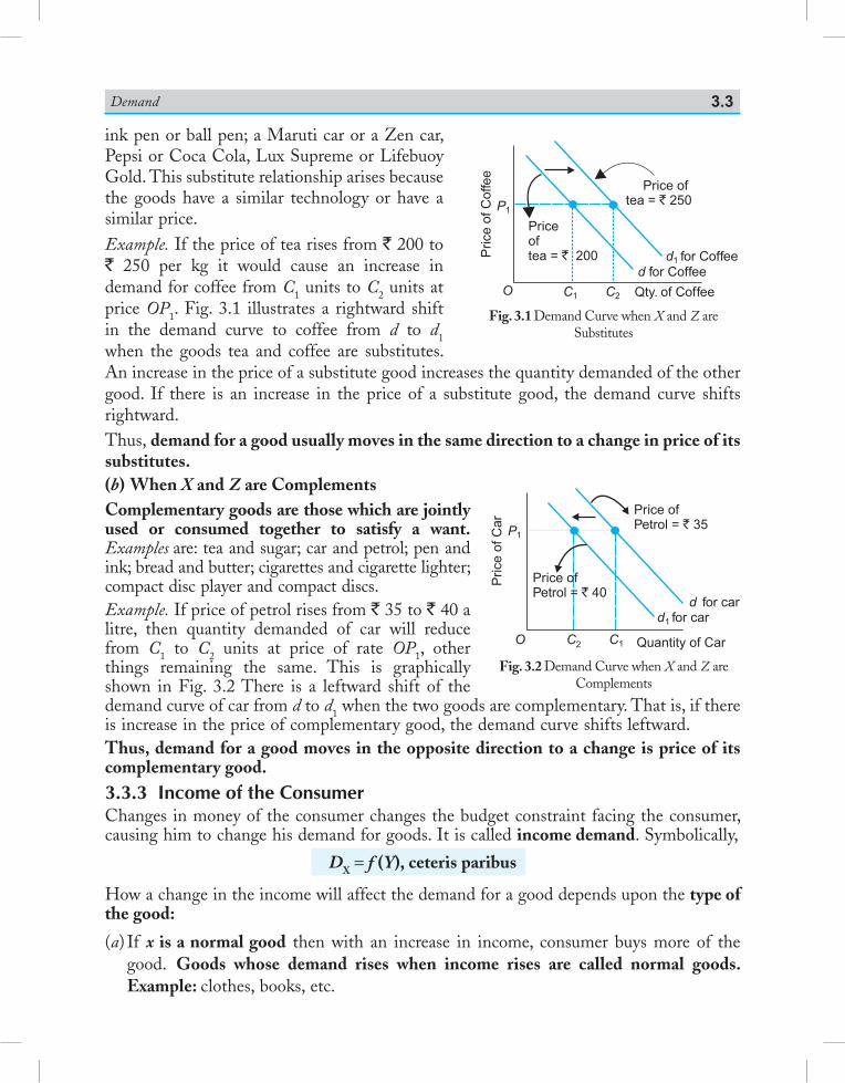
Demand 3.3
ink pen or ball pen; a Maruti car or a Zen car, Pepsi or Coca Cola, Lux Supreme or Lifebuoy Gold. This substitute relationship arises because the goods have a similar technology or have a similar price.Example. If the price of tea rises from ` 200 to ` 250 per kg it would cause an increase in demand for coffee from C1 units to C2 units at price OP1. Fig. 3.1 illustrates a rightward shift in the demand curve to coffee from d to d1 when the goods tea and coffee are substitutes. An increase in the price of a substitute good increases the quantity demanded of the other good. If there is an increase in the price of a substitute good, the demand curve shifts rightward.Thus, demand for a good usually moves in the same direction to a change in price of its substitutes.(b) When X and Z are ComplementsComplementary goods are those which are jointly used or consumed together to satisfy a want. Examples are: tea and sugar; car and petrol; pen and ink; bread and butter; cigarettes and cigarette lighter; compact disc player and compact discs.Example. If price of petrol rises from ` 35 to ` 40 a litre, then quantity demanded of car will reduce from C1 to C2 units at price of rate OP1, other things remaining the same. This is graphically shown in Fig. 3.2 There is a leftward shift of the demand curve of car from d to d1 when the two goods are complementary. That is, if there is increase in the price of complementary good, the demand curve shifts leftward. Thus, demand for a good moves in the opposite direction to a change is price of its complementary good.3.3.3 Income of the ConsumerChanges in money of the consumer changes the budget constraint facing the consumer, causing him to change his demand for goods. It is called income demand. Symbolically,
DX = f (Y), ceteris paribus
How a change in the income will affect the demand for a good depends upon the type of the good:
(a) If x is a normal good then with an increase in income, consumer buys more of the good. Goods whose demand rises when income rises are called normal goods. Example: clothes, books, etc.
Fig. 3.2 Demand Curve when X and Z are Complements
Fig. 3.1 Demand Curve when X and Z are Substitutes
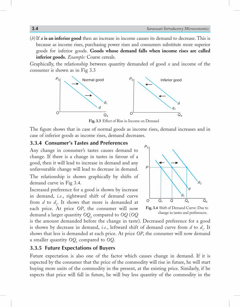
Saraswati Introductory Microeconomics3.4
(b) If x is an inferior good then an increase in income causes its demand to decrease. This is because as income rises, purchasing power rises and consumers substitute more superior goods for inferior goods. Goods whose demand falls when income rises are called inferior goods. Example: Coarse cereals.
Graphically, the relationship between quantity demanded of good x and income of the consumer is shown as in Fig 3.3
Fig. 3.3 Effect of Rise in Income on Demand
OQX
d
d1
PX Normal good Inferior goodPX
O QX
d1
d
The figure shows that in case of normal goods as income rises, demand increases and in case of inferior goods as income rises, demand decreases.
3.3.4 Consumer’s Tastes and PreferencesAny change in consumer’s tastes causes demand to change. If there is a change in tastes in favour of a good, then it will lead to increase in demand and any unfavourable change will lead to decrease in demand.The relationship is shown graphically by shifts of demand curve in Fig 3.4.Increased preference for a good is shown by increase in demand, i.e., rightward shift of demand curve from d to d2. It shows that more is demanded at each price. At price OP, the consumer will now demand a larger quantity OQ2 compared to OQ (OQ is the amount demanded before the change in taste). Decreased preference for a good is shown by decrease in demand, i.e., leftward shift of demand curve from d to d1. It shows that less is demanded at each price. At price OP, the consumer will now demand a smaller quantity OQ1 compared to OQ.
3.3.5 Future Expectations of BuyersFuture expectation is also one of the factor which causes change in demand. If it is expected by the consumer that the price of the commodity will rise in future, he will start buying more units of the commodity in the present, at the existing price. Similarly, if he expects that price will fall in future, he will buy less quantity of the commodity in the
Fig. 3.4 Shift of Demand Curve: Due to change in tastes and preferences.
PX
P
O QX
d1
d
d
Q Q2
Q1
2
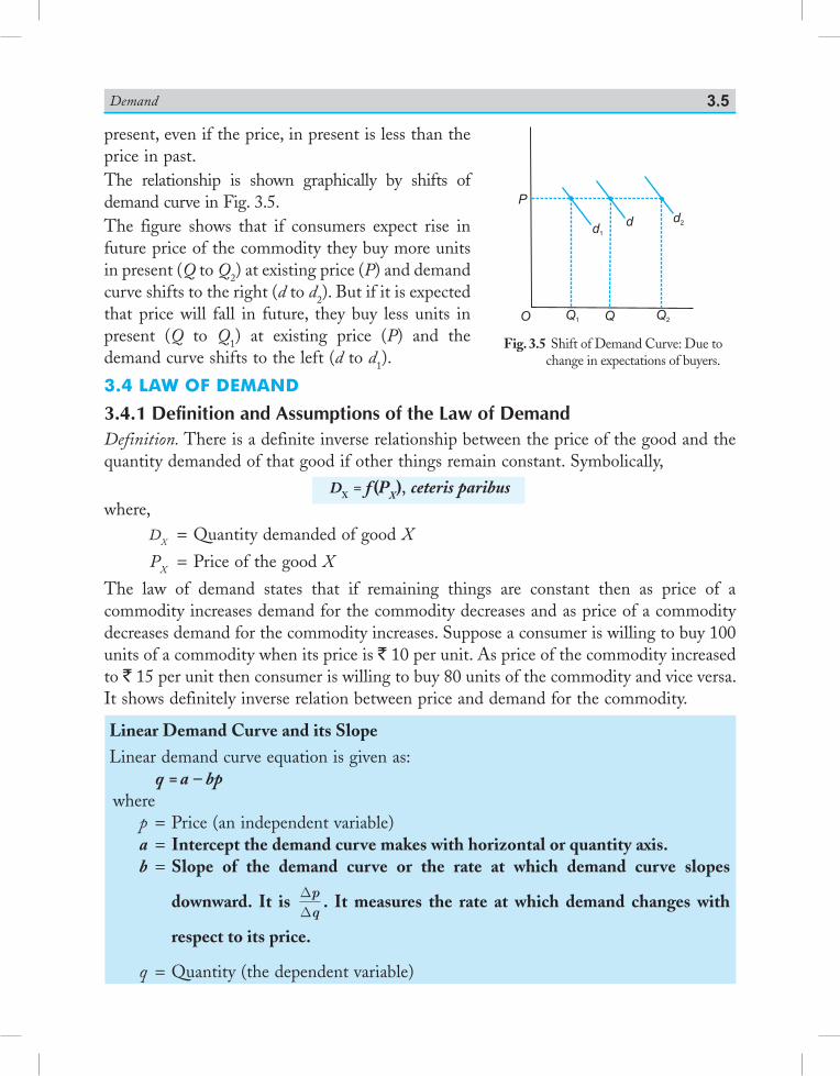
Demand 3.5
present, even if the price, in present is less than the price in past.The relationship is shown graphically by shifts of demand curve in Fig. 3.5.The figure shows that if consumers expect rise in future price of the commodity they buy more units in present (Q to Q2) at existing price (P) and demand curve shifts to the right (d to d2). But if it is expected that price will fall in future, they buy less units in present (Q to Q1) at existing price (P) and the demand curve shifts to the left (d to d1).
3.4 law of deMand
3.4.1 Definition and Assumptions of the Law of DemandDefinition. There is a definite inverse relationship between the price of the good and the quantity demanded of that good if other things remain constant. Symbolically,
DX = f (PX), ceteris paribuswhere, DX = Quantity demanded of good X
PX = Price of the good X
The law of demand states that if remaining things are constant then as price of a commodity increases demand for the commodity decreases and as price of a commodity decreases demand for the commodity increases. Suppose a consumer is willing to buy 100 units of a commodity when its price is ` 10 per unit. As price of the commodity increased to ` 15 per unit then consumer is willing to buy 80 units of the commodity and vice versa. It shows definitely inverse relation between price and demand for the commodity.
Linear Demand Curve and its SlopeLinear demand curve equation is given as: q = a – bpwhere p = Price (an independent variable) a = Intercept the demand curve makes with horizontal or quantity axis. b = Slope of the demand curve or the rate at which demand curve slopes
downward. It is DDpq
. It measures the rate at which demand changes with
respect to its price.
q = Quantity (the dependent variable)
P
O
d2dd1
Q2QQ1
Fig. 3.5 Shift of Demand Curve: Due to change in expectations of buyers.
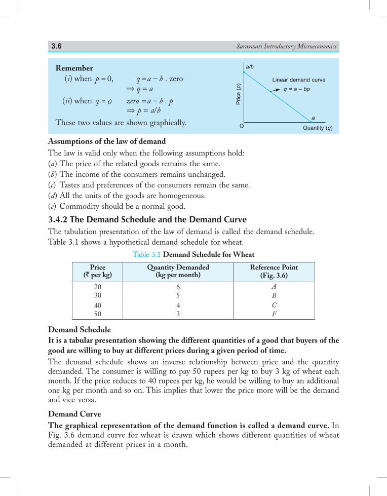
Saraswati Introductory Microeconomics3.6
Remember (i) when p = 0, q = a – b . zero ⇒ q = a
(ii) when q = 0 zero = a – b . p ⇒ p = a/b
These two values are shown graphically.
Assumptions of the law of demandThe law is valid only when the following assumptions hold:(a) The price of the related goods remains the same.(b) The income of the consumers remains unchanged.(c) Tastes and preferences of the consumers remain the same.(d) All the units of the goods are homogeneous.(e) Commodity should be a normal good.
3.4.2 The Demand Schedule and the Demand CurveThe tabulation presentation of the law of demand is called the demand schedule. Table 3.1 shows a hypothetical demand schedule for wheat.
Table 3.1 Demand Schedule for Wheat
Price (` per kg)
Quantity Demanded (kg per month)
Reference Point (Fig. 3.6)
2030
65
AB
4050
43
CF
Demand ScheduleIt is a tabular presentation showing the different quantities of a good that buyers of the good are willing to buy at different prices during a given period of time.The demand schedule shows an inverse relationship between price and the quantity demanded. The consumer is willing to pay 50 rupees per kg to buy 3 kg of wheat each month. If the price reduces to 40 rupees per kg, he would be willing to buy an additional one kg per month and so on. This implies that lower the price more will be the demand and vice-versa.
Demand CurveThe graphical representation of the demand function is called a demand curve. In Fig. 3.6 demand curve for wheat is drawn which shows different quantities of wheat demanded at different prices in a month.
Linear demand curveq = a – bp
Quantity (q)
Pric
e (p
)
a/b
Oa
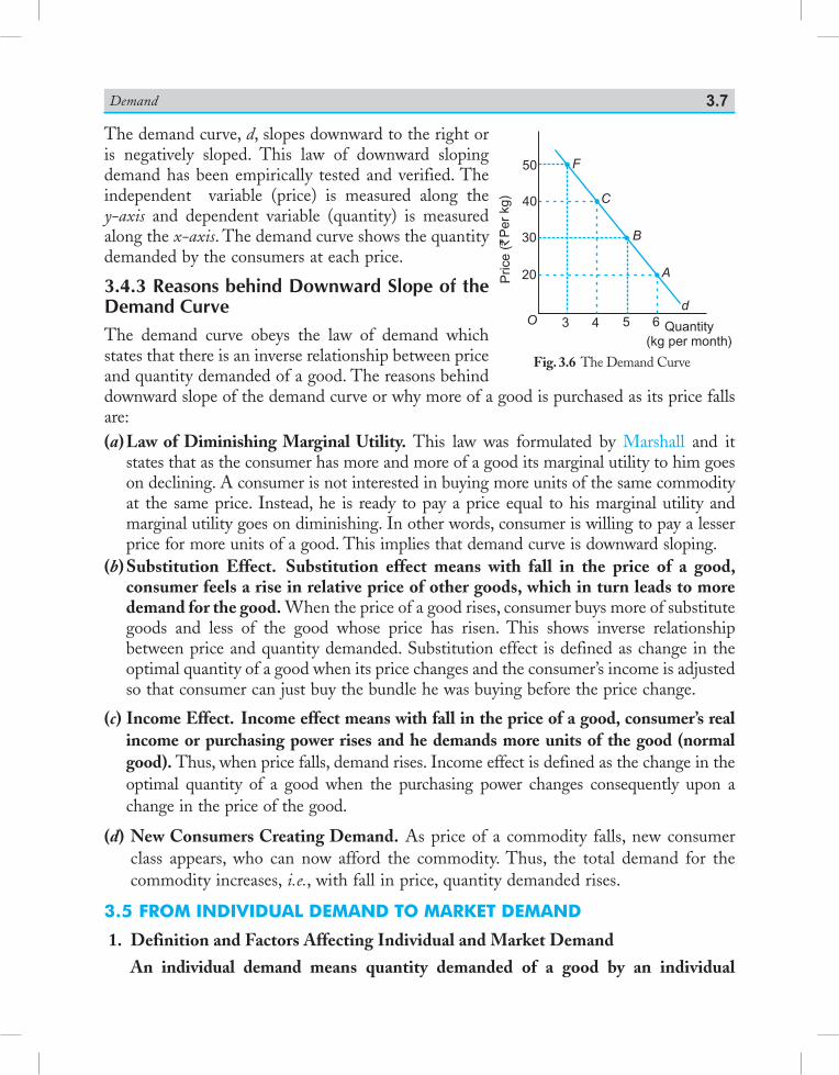
Demand 3.7
The demand curve, d, slopes downward to the right or is negatively sloped. This law of downward sloping demand has been empirically tested and verified. The independent variable (price) is measured along the y-axis and dependent variable (quantity) is measured along the x-axis. The demand curve shows the quantity demanded by the consumers at each price.
3.4.3 Reasons behind Downward Slope of the Demand CurveThe demand curve obeys the law of demand which states that there is an inverse relationship between price and quantity demanded of a good. The reasons behind downward slope of the demand curve or why more of a good is purchased as its price falls are:(a) Law of Diminishing Marginal Utility. This law was formulated by Marshall and it
states that as the consumer has more and more of a good its marginal utility to him goes on declining. A consumer is not interested in buying more units of the same commodity at the same price. Instead, he is ready to pay a price equal to his marginal utility and marginal utility goes on diminishing. In other words, consumer is willing to pay a lesser price for more units of a good. This implies that demand curve is downward sloping.
(b) Substitution Effect. Substitution effect means with fall in the price of a good, consumer feels a rise in relative price of other goods, which in turn leads to more demand for the good. When the price of a good rises, consumer buys more of substitute goods and less of the good whose price has risen. This shows inverse relationship between price and quantity demanded. Substitution effect is defined as change in the optimal quantity of a good when its price changes and the consumer’s income is adjusted so that consumer can just buy the bundle he was buying before the price change.
(c) Income Effect. Income effect means with fall in the price of a good, consumer’s real income or purchasing power rises and he demands more units of the good (normal good). Thus, when price falls, demand rises. Income effect is defined as the change in the optimal quantity of a good when the purchasing power changes consequently upon a change in the price of the good.
(d) New Consumers Creating Demand. As price of a commodity falls, new consumer class appears, who can now afford the commodity. Thus, the total demand for the commodity increases, i.e., with fall in price, quantity demanded rises.
3.5 froM individual deMand to Market deMand
1. Definition and Factors Affecting Individual and Market Demand
An individual demand means quantity demanded of a good by an individual
Fig. 3.6 The Demand Curve
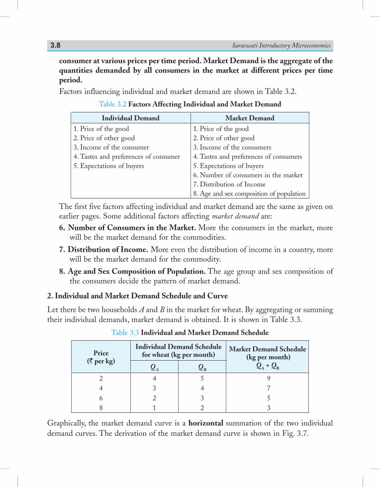
Saraswati Introductory Microeconomics3.8
consumer at various prices per time period. Market Demand is the aggregate of the quantities demanded by all consumers in the market at different prices per time period.
Factors influencing individual and market demand are shown in Table 3.2.
Table 3.2 Factors Affecting Individual and Market Demand
Individual Demand Market Demand
1. Price of the good2. Price of other good3. Income of the consumer4. Tastes and preferences of consumer5. Expectations of buyers
1. Price of the good2. Price of other good3. Income of the consumers4. Tastes and preferences of consumers5. Expectations of buyers6. Number of consumers in the market7. Distribution of Income8. Age and sex composition of population
The first five factors affecting individual and market demand are the same as given on earlier pages. Some additional factors affecting market demand are:6. Number of Consumers in the Market. More the consumers in the market, more
will be the market demand for the commodities.
7. Distribution of Income. More even the distribution of income in a country, more will be the market demand for the commodity.
8. Age and Sex Composition of Population. The age group and sex composition of the consumers decide the pattern of market demand.
2. Individual and Market Demand Schedule and Curve
Let there be two households A and B in the market for wheat. By aggregating or summing their individual demands, market demand is obtained. It is shown in Table 3.3.
Table 3.3 Individual and Market Demand Schedule
Price (` per kg)
Individual Demand Schedule for wheat (kg per month)
Market Demand Schedule (kg per month)
QA + QBQ A Q B2468
4321
5 4 32
9 7
5 3
Graphically, the market demand curve is a horizontal summation of the two individual demand curves. The derivation of the market demand curve is shown in Fig. 3.7.
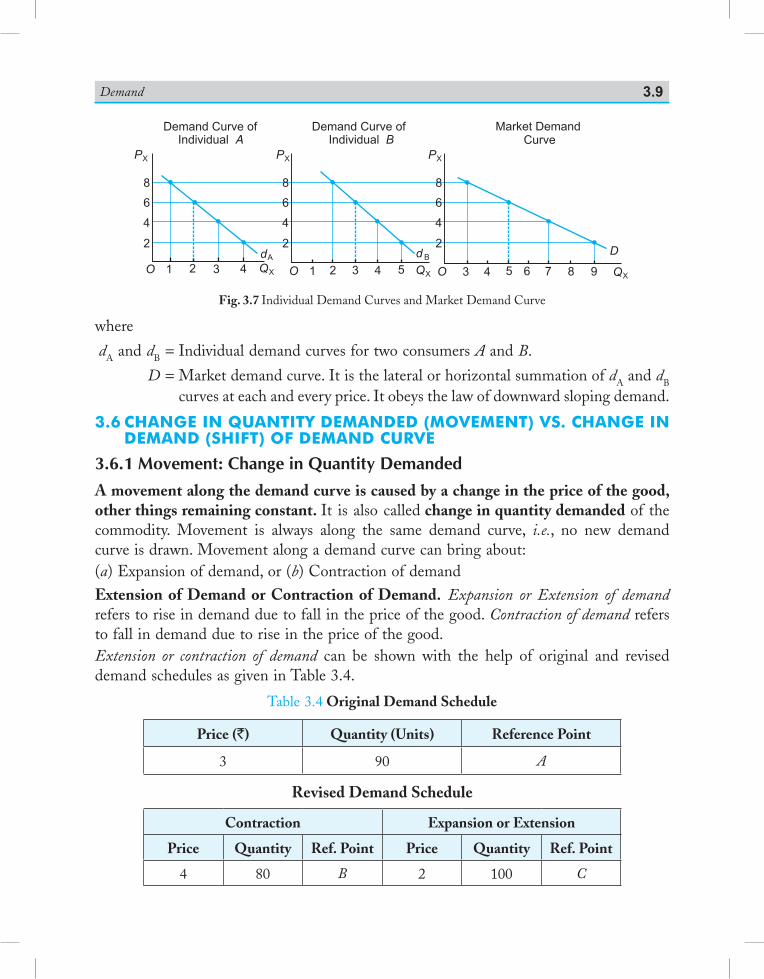
Demand 3.9
Fig. 3.7 Individual Demand Curves and Market Demand Curve
where
dA and dB = Individual demand curves for two consumers A and B.
D = Market demand curve. It is the lateral or horizontal summation of dA and dB curves at each and every price. It obeys the law of downward sloping demand.
3.6 change in Quantity deManded (MoveMent) vs. change in deMand (shift) of deMand curve
3.6.1 Movement: Change in Quantity DemandedA movement along the demand curve is caused by a change in the price of the good, other things remaining constant. It is also called change in quantity demanded of the commodity. Movement is always along the same demand curve, i.e., no new demand curve is drawn. Movement along a demand curve can bring about:(a) Expansion of demand, or (b) Contraction of demandExtension of Demand or Contraction of Demand. Expansion or Extension of demand refers to rise in demand due to fall in the price of the good. Contraction of demand refers to fall in demand due to rise in the price of the good.Extension or contraction of demand can be shown with the help of original and revised demand schedules as given in Table 3.4.
Table 3.4 Original Demand Schedule
Price (`) Quantity (Units) Reference Point
3 90 A
Revised Demand Schedule
Contraction Expansion or Extension
Price Quantity Ref. Point Price Quantity Ref. Point
4 80 B 2 100 C
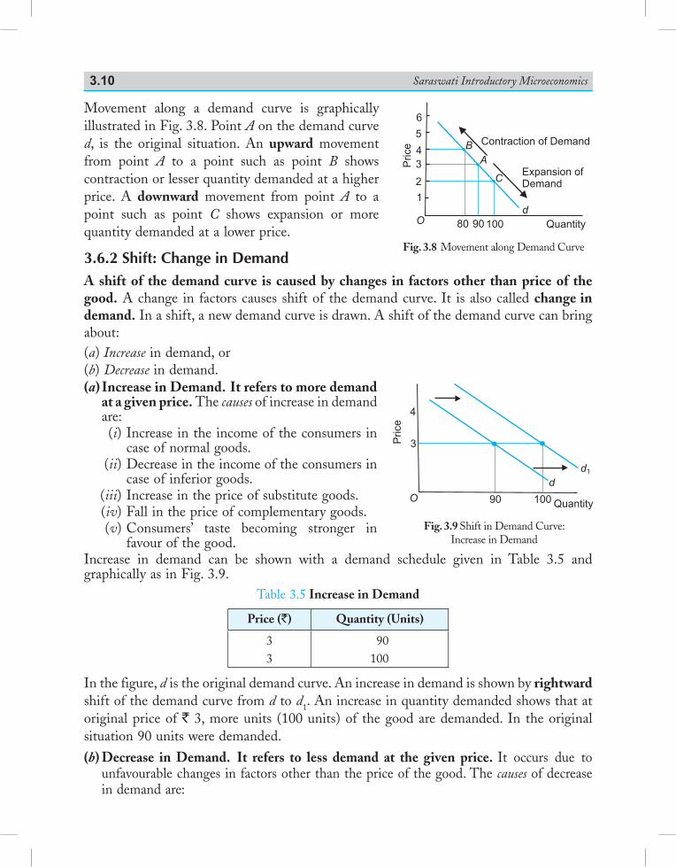
Saraswati Introductory Microeconomics3.10
Movement along a demand curve is graphically illustrated in Fig. 3.8. Point A on the demand curve d, is the original situation. An upward movement from point A to a point such as point B shows contraction or lesser quantity demanded at a higher price. A downward movement from point A to a point such as point C shows expansion or more quantity demanded at a lower price.
3.6.2 Shift: Change in DemandA shift of the demand curve is caused by changes in factors other than price of the good. A change in factors causes shift of the demand curve. It is also called change in demand. In a shift, a new demand curve is drawn. A shift of the demand curve can bring about:(a) Increase in demand, or(b) Decrease in demand.(a) Increase in Demand. It refers to more demand
at a given price. The causes of increase in demand are:
(i) Increase in the income of the consumers in case of normal goods.
(ii) Decrease in the income of the consumers in case of inferior goods.
(iii) Increase in the price of substitute goods. (iv) Fall in the price of complementary goods. (v) Consumers’ taste becoming stronger in
favour of the good.Increase in demand can be shown with a demand schedule given in Table 3.5 and graphically as in Fig. 3.9.
Table 3.5 Increase in Demand
Price (`) Quantity (Units)
33
90100
In the figure, d is the original demand curve. An increase in demand is shown by rightward shift of the demand curve from d to d1. An increase in quantity demanded shows that at original price of ` 3, more units (100 units) of the good are demanded. In the original situation 90 units were demanded.
(b) Decrease in Demand. It refers to less demand at the given price. It occurs due to unfavourable changes in factors other than the price of the good. The causes of decrease in demand are:
Fig. 3.9 Shift in Demand Curve:Increase in Demand
Price
4
3
O 90 100
d1
d
Quantity
Fig. 3.8 Movement along Demand Curve
6
B
A
C
100 Quantity
Expansion of
Demand
Contraction of Demand
Price
9080
5
4
3
2
1
O
d
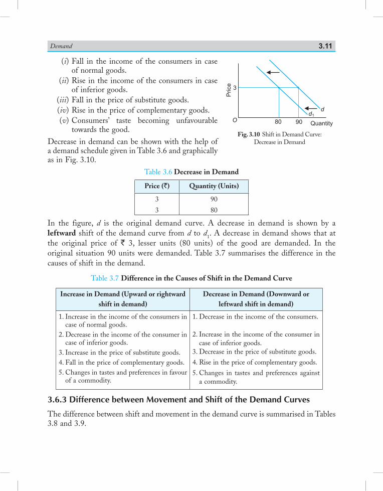
Demand 3.11
(i) Fall in the income of the consumers in case of normal goods.
(ii) Rise in the income of the consumers in case of inferior goods.
(iii) Fall in the price of substitute goods. (iv) Rise in the price of complementary goods. (v) Consumers’ taste becoming unfavourable
towards the good.
Decrease in demand can be shown with the help of a demand schedule given in Table 3.6 and graphically as in Fig. 3.10.
Table 3.6 Decrease in Demand
Price (`) Quantity (Units)
3
3
90
80
In the figure, d is the original demand curve. A decrease in demand is shown by a leftward shift of the demand curve from d to d1. A decrease in demand shows that at the original price of ` 3, lesser units (80 units) of the good are demanded. In the original situation 90 units were demanded. Table 3.7 summarises the difference in the causes of shift in the demand.
Table 3.7 Difference in the Causes of Shift in the Demand Curve
Increase in Demand (Upward or rightward shift in demand)
Decrease in Demand (Downward or leftward shift in demand)
1. Increase in the income of the consumers in case of normal goods.
2. Decrease in the income of the consumer in case of inferior goods.
3. Increase in the price of substitute goods.4. Fall in the price of complementary goods.5. Changes in tastes and preferences in favour
of a commodity.
1. Decrease in the income of the consumers.
2. Increase in the income of the consumer in case of inferior goods.
3. Decrease in the price of substitute goods.
4. Rise in the price of complementary goods.
5. Changes in tastes and preferences against a commodity.
3.6.3 Difference between Movement and Shift of the Demand Curves
The difference between shift and movement in the demand curve is summarised in Tables 3.8 and 3.9.
Fig. 3.10 Shift in Demand Curve: Decrease in Demand
Price
3
80 90 QuantityO
d1
d
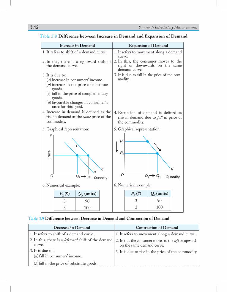
Saraswati Introductory Microeconomics3.12
Table 3.8 Difference between Increase in Demand and Expansion of Demand
Increase in Demand Expansion of Demand
1. It refers to shift of a demand curve.
2. In this, there is a rightward shift of the demand curve.
3. It is due to:(a) increase in consumers’ income.(b) increase in the price of substitute
goods.(c) fall in the price of complementary
goods.(d) favourable changes in consumer’ s
taste for this good.4. Increase in demand is defined as the
rise in demand at the same price of the commodity.
1. It refers to movement along a demand curve.
2. In this, the consumer moves to the right or downwards on the same demand curve.
3. It is due to fall in the price of the com-modity.
4. Expansion of demand is defined as rise in demand due to fall in price of the commodity.
5. Graphical representation:
Price
QuantityQ1
d1d
Q2
P
O
6. Numerical example:
PX (`) QX (units)
33
90100
5. Graphical representation:
QuantityQO Q
P1
P2
d
1 2
6. Numerical example:
PX (`) QX (units)
32
90100
Table 3.9 Difference between Decrease in Demand and Contraction of Demand
Decrease in Demand Contraction of Demand
1. It refers to shift of a demand curve.2. In this. there is a leftward shift of the demand
curve.3. It is due to:
(a) fall in consumers’ income.
(b) fall in the price of substitute goods.
1. It refers to movement along a demand curve.
2. In this the consumer moves to the left or upwards on the same demand curve.
3. It is due to rise in the price of the commodity.
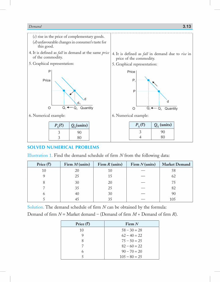
Demand 3.13
(c) rise in the price of complementary goods.(d) unfavourable changes in consumer’s taste for
this good.
4. It is defined as fall in demand at the same price of the commodity.
5. Graphical representation:
4. It is defined as fall in demand due to rise in price of the commodity.
5. Graphical representation:
6. Numerical example:
PX(`) QX(units)
33
9080
6. Numerical example:
PX (`) QX (units)
34
9080
SoLveD NuMeRiCAL PRobLeMS
Illustration 1. Find the demand schedule of firm N from the following data:
Price (`) Firm M (units) Firm R (units) Firm N (units) Market Demand
109
2025
1015
——
5862
8765
30354045
20253035
————
758290
105
Solution. The demand schedule of firm N can be obtained by the formula:
Demand of firm N = Market demand – (Demand of firm M + Demand of firm R).
Price (`) Firm N
1098765
58 – 30 = 2862 – 40 = 2275 – 50 = 2582 – 60 = 2290 – 70 = 20
105 – 80 = 25
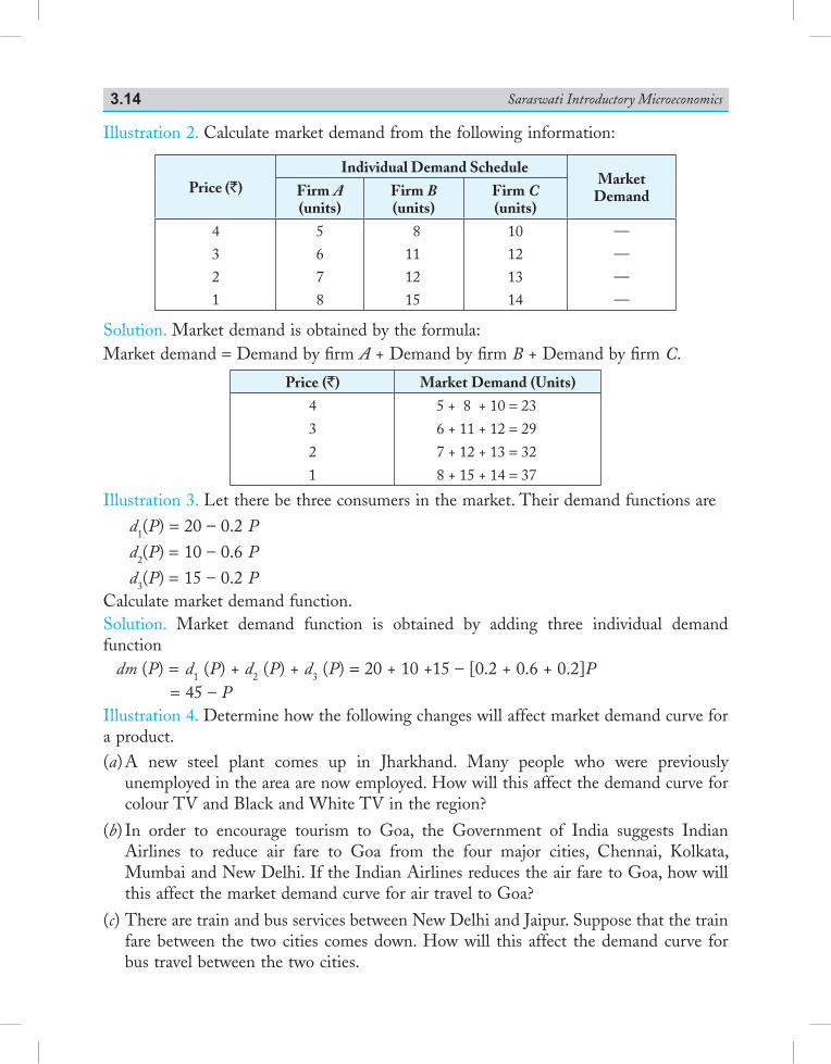
Saraswati Introductory Microeconomics3.14
Illustration 2. Calculate market demand from the following information:
Price (`)Individual Demand Schedule
Market DemandFirm A
(units)Firm B (units)
Firm C (units)
4
3
2
1
5
6
7
8
8
11
12
15
10
12
13
14
—
—
—
—
Solution. Market demand is obtained by the formula:Market demand = Demand by firm A + Demand by firm B + Demand by firm C.
Price (`) Market Demand (Units)
4
3
2
1
5 + 8 + 10 = 23
6 + 11 + 12 = 29
7 + 12 + 13 = 32
8 + 15 + 14 = 37
Illustration 3. Let there be three consumers in the market. Their demand functions ared1(P) = 20 – 0.2 Pd2(P) = 10 – 0.6 Pd3(P) = 15 – 0.2 P
Calculate market demand function.Solution. Market demand function is obtained by adding three individual demand function
dm (P) = d1 (P) + d2 (P) + d3 (P) = 20 + 10 +15 – [0.2 + 0.6 + 0.2]P = 45 – P
Illustration 4. Determine how the following changes will affect market demand curve for a product.(a) A new steel plant comes up in Jharkhand. Many people who were previously
unemployed in the area are now employed. How will this affect the demand curve for colour TV and Black and White TV in the region?
(b) In order to encourage tourism to Goa, the Government of India suggests Indian Airlines to reduce air fare to Goa from the four major cities, Chennai, Kolkata, Mumbai and New Delhi. If the Indian Airlines reduces the air fare to Goa, how will this affect the market demand curve for air travel to Goa?
(c) There are train and bus services between New Delhi and Jaipur. Suppose that the train fare between the two cities comes down. How will this affect the demand curve for bus travel between the two cities.
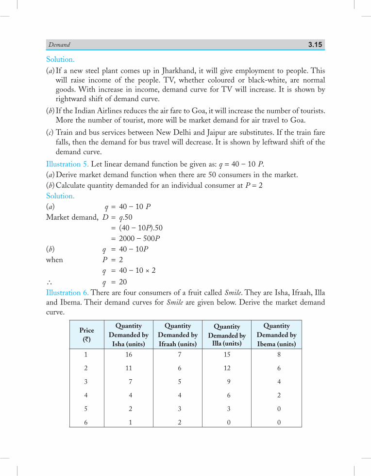
Demand 3.15
Solution.(a) If a new steel plant comes up in Jharkhand, it will give employment to people. This
will raise income of the people. TV, whether coloured or black-white, are normal goods. With increase in income, demand curve for TV will increase. It is shown by rightward shift of demand curve.
(b) If the Indian Airlines reduces the air fare to Goa, it will increase the number of tourists. More the number of tourist, more will be market demand for air travel to Goa.
(c) Train and bus services between New Delhi and Jaipur are substitutes. If the train fare falls, then the demand for bus travel will decrease. It is shown by leftward shift of the demand curve.
Illustration 5. Let linear demand function be given as: q = 40 – 10 P. (a) Derive market demand function when there are 50 consumers in the market.(b) Calculate quantity demanded for an individual consumer at P = 2Solution.(a) q = 40 – 10 PMarket demand, D = q.50 = (40 – 10P).50 = 2000 – 500P(b) q = 40 – 10Pwhen P = 2 q = 40 – 10 × 2∴ q = 20 Illustration 6. There are four consumers of a fruit called Smile. They are Isha, Ifraah, Illa and Ibema. Their demand curves for Smile are given below. Derive the market demand curve.
Price (`)
QuantityDemanded by
Isha (units)
QuantityDemanded byIfraah (units)
QuantityDemanded by
Illa (units)
QuantityDemanded byIbema (units)
1
2
3
4
5
6
16
11
7
4
2
1
7
6
5
4
3
2
15
12
9
6
3
0
8
6
4
2
0
0
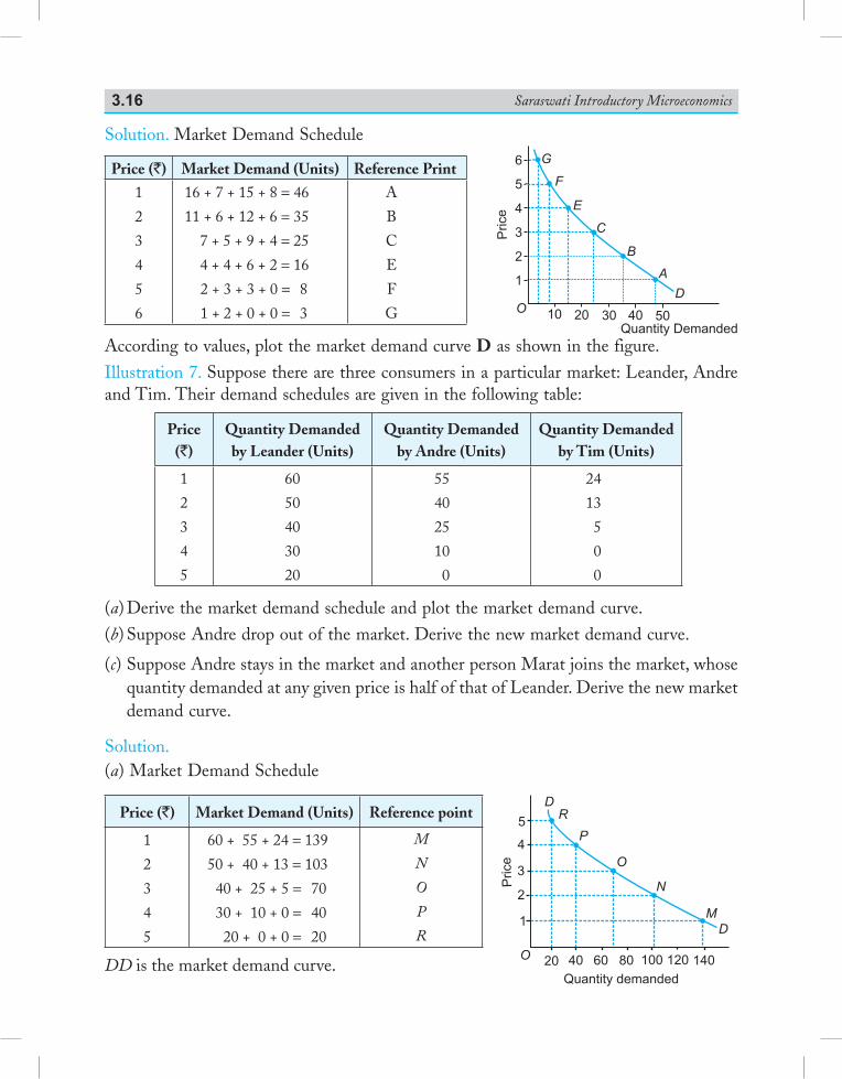
Saraswati Introductory Microeconomics3.16
Solution. Market Demand Schedule
Price (`) Market Demand (Units) Reference Print
1
2
3
4
5
6
16 + 7 + 15 + 8 = 46
11 + 6 + 12 + 6 = 35
7 + 5 + 9 + 4 = 25
4 + 4 + 6 + 2 = 16
2 + 3 + 3 + 0 = 8
1 + 2 + 0 + 0 = 3
A
B
C
E
F
G
According to values, plot the market demand curve D as shown in the figure.Illustration 7. Suppose there are three consumers in a particular market: Leander, Andre and Tim. Their demand schedules are given in the following table:
Price(`)
Quantity Demanded by Leander (Units)
Quantity Demanded by Andre (Units)
Quantity Demandedby Tim (Units)
1
2
3
4
5
60
50
40
30
20
55
40
25
10
0
24
13
5
0
0
(a) Derive the market demand schedule and plot the market demand curve.(b) Suppose Andre drop out of the market. Derive the new market demand curve.
(c) Suppose Andre stays in the market and another person Marat joins the market, whose quantity demanded at any given price is half of that of Leander. Derive the new market demand curve.
Solution.(a) Market Demand Schedule
Price (`) Market Demand (Units) Reference point
1
2
3
4
5
60 + 55 + 24 = 139
50 + 40 + 13 = 103
40 + 25 + 5 = 70
30 + 10 + 0 = 40
20 + 0 + 0 = 20
M
N
O
P
R
DD is the market demand curve.
D
Price
R
P
O
N
M
D
Quantity demanded
1
2
3
4
5
20O
40 60 80 100 120 140
D
Price
F
E
C
B
A
Quantity Demanded
1
2
3
4
5
10O
20 30 40 50
6 G
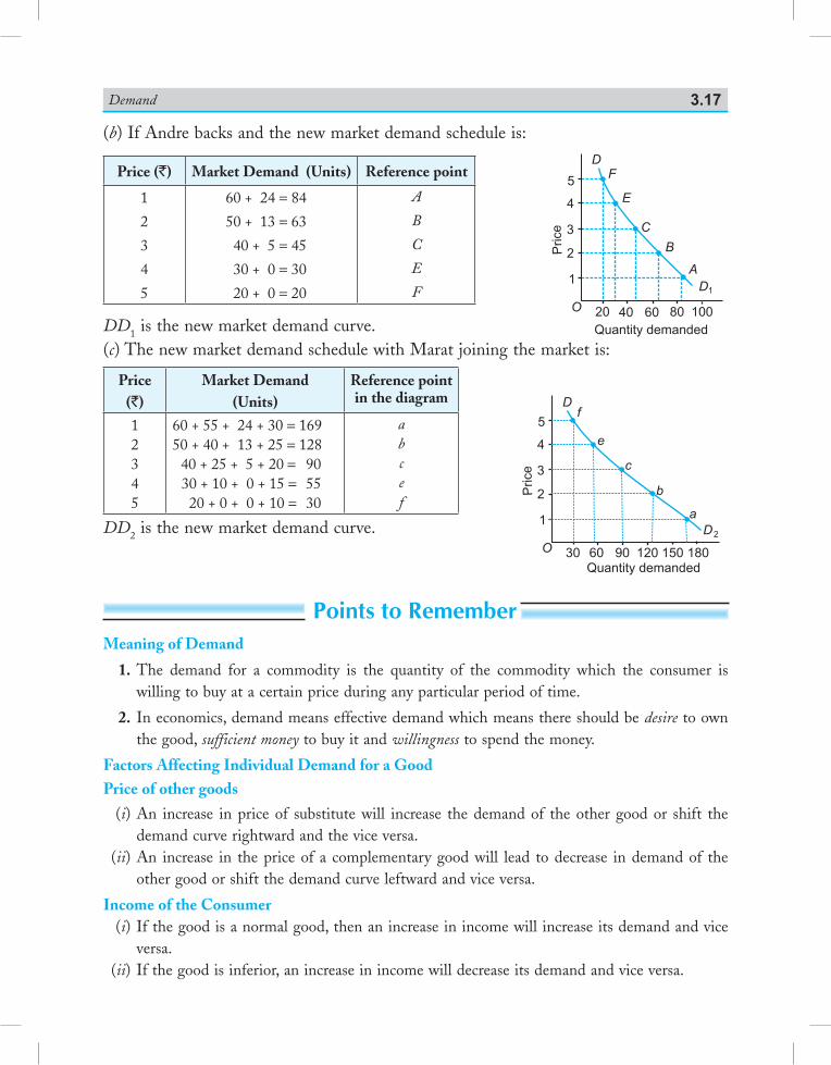
Demand 3.17
(b) If Andre backs and the new market demand schedule is:
Price (`) Market Demand (Units) Reference point
1
2
3
4
5
60 + 24 = 84
50 + 13 = 63
40 + 5 = 45
30 + 0 = 30
20 + 0 = 20
A
B
C
E
F
DD1 is the new market demand curve.(c) The new market demand schedule with Marat joining the market is:
Price(`)
Market Demand(Units)
Reference pointin the diagram
12345
60 + 55 + 24 + 30 = 16950 + 40 + 13 + 25 = 128
40 + 25 + 5 + 20 = 9030 + 10 + 0 + 15 = 5520 + 0 + 0 + 10 = 30
abcef
DD2 is the new market demand curve.
Points to RememberMeaning of Demand
1. The demand for a commodity is the quantity of the commodity which the consumer is willing to buy at a certain price during any particular period of time.
2. In economics, demand means effective demand which means there should be desire to own the good, sufficient money to buy it and willingness to spend the money.
Factors Affecting Individual Demand for a GoodPrice of other goods
(i) An increase in price of substitute will increase the de mand of the other good or shift the demand curve rightward and the vice versa.
(ii) An increase in the price of a complementary good will lead to decrease in demand of the other good or shift the demand curve leftward and vice versa.
Income of the Consumer (i) If the good is a normal good, then an increase in income will increase its demand and vice
versa. (ii) If the good is inferior, an increase in income will decrease its demand and vice versa.
D
Price
F
E
C
B
A
D1
Quantity demanded
1
2
3
4
5
20O40 60 80 100
D
Price
f
e
c
b
D2
Quantity demanded
1
2
3
4
5
30O 60 90 120 150 180
a
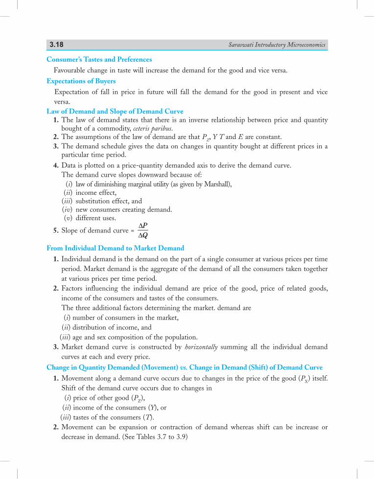
Saraswati Introductory Microeconomics3.18
Consumer’s Tastes and PreferencesFavourable change in taste will increase the demand for the good and vice versa.
Expectations of Buyers Expectation of fall in price in future will fall the demand for the good in present and vice
versa. Law of Demand and Slope of Demand Curve 1. The law of demand states that there is an inverse relationship between price and quantity
bought of a commodity, ceteris paribus. 2. The assumptions of the law of demand are that PZ, Y T and E are constant. 3. The demand schedule gives the data on changes in quantity bought at different prices in a
particular time period. 4. Data is plotted on a price-quantity demanded axis to derive the demand curve. The demand curve slopes downward because of: (i) law of diminishing marginal utility (as given by Marshall), (ii) income effect, (iii) substitution effect, and (iv) new consumers creating demand. (v) different uses.
5. Slope of demand curve = PQ
∆∆
From Individual Demand to Market Demand 1. Individual demand is the demand on the part of a single consumer at various prices per time
period. Market demand is the aggregate of the demand of all the consumers taken together at various prices per time period.
2. Factors influencing the individual demand are price of the good, price of related goods, income of the consumers and tastes of the consumers.
The three additional factors determining the market. demand are (i) number of consumers in the market, (ii) distribution of income, and (iii) age and sex composition of the population. 3. Market demand curve is constructed by horizontally summing all the individual demand
curves at each and every price.
Change in Quantity Demanded (Movement) vs. Change in Demand (Shift) of Demand Curve 1. Movement along a demand curve occurs due to changes in the price of the good (PX) itself. Shift of the demand curve occurs due to changes in (i) price of other good (PZ), (ii) income of the consumers (Y), or (iii) tastes of the consumers (T). 2. Movement can be expansion or contraction of demand whereas shift can be increase or
decrease in demand. (See Tables 3.7 to 3.9)
Demand 3.19
Test Your KnowledgeVery Short Answer Type Questions (1 Mark)
1. What is demand for a commodity? 2. Define law of demand. What are the underlying assumptions? 3. What are substitute goods? 4. Define individual demand curve. 5. Define market demand curve. 6. Define inferior goods. 7. When does a consumer buy less of a commodity at a given price? 8. If the demand for good Y increases as the price of another good X rises, how are the two
goods related? 9. If the quantity demanded of a commodity X decreases as the household income in creas es,
what type of good is X? 10. What happens to the demand for a substitute good when the price of the commodity falls? 11. State any one factor that causes an increase in the demand of a good. 12. What is meant by inferior good in economics? (AI 2010, Delhi 2012) 13. When is a good called a normal good? (AI 2006, 08; Delhi 2012) 14. When demand for a good falls due to rise in its own price, what is the change in demand
called? 15. What is decrease in demand/increase in demand? 16. Why is demand for water inelastic? (Delhi 2010) 17. What is meant by demand in economics? (Foreign 2010) 18. Define market demand. (Delhi, Foreign 2011)
or What is market demand? (Delhi 2012, AI 2012) 19. Give one reason for a shift in demand curve. (AI 2012) 20. Give the meaning of market demand. (Delhi 2013) 21. What does a rightward shift of demand curve indicate? (AI 2013) 22. Give one reason for a rightward shift of demand curve. (Foreign 2013) 23. Give one reason for a leftward shift in demand curve. (Foreign 2013) 24. What is a normal good? (Foreign 2013) 25. When does ‘increase’ in demand take place? (Delhi 2016)
26. When does ‘change in demand’ take place? (AI 2016)
27. State the law of demand. (Foreign 2017) 28. Define market demand. (Delhi 2017)
Saraswati Introductory Microeconomics3.20
Multiple Choice Questions
1. What kind of relationship exists between demand for a good and price of its substitute goods?
(a) Direct (b) Inverse (c) No effect (d) Can be direct or inverse
2. What kind of relationship exists between price of a good and demand of its complementary good?
(a) Direct (b) Inverse (c) No effect (d) Can be direct or inverse
3. What kind of relationship exists between income and demand of inferior good? (a) Direct (b) Inverse (c) No effect (d) Can be direct or inverse
4. What kind of relationship exists between income and demand of a normal good? (a) Direct (b) Inverse (c) No effect (d) Can be direct or inverse
5. How is law of demand expressed functionally? (a) DX = f (PX), ceteris paribus
(b) DX = f (PZ), ceteris paribus
(c) DX = f (Y), ceteris paribus
(d) DX = f (T), ceteris paribus
6. When demand curve is downward sloping, its slope is: (a) Negative (b) Positive (c) Constant (d) Zero
7. Income effect states that as price of a good falls, demand rises because there is rise in: (a) Money income (b) Real income (c) Relative price of other goods (d) Marginal utility
8. Substitution effect states that as price of a good falls, demand rises because there is rise in: (a) Money income (b) Real income (c) Relative price of other goods (d) Marginal utility
9. Giffen good is: (a) An inferior good (b) One with high negative income elasticity of demand (c) Consumed by low-paid workers (d) All of the above
10. Veblan good is: (a) Good of status (b) Consumed by very high income group (c) Like diamonds (d) All of the above
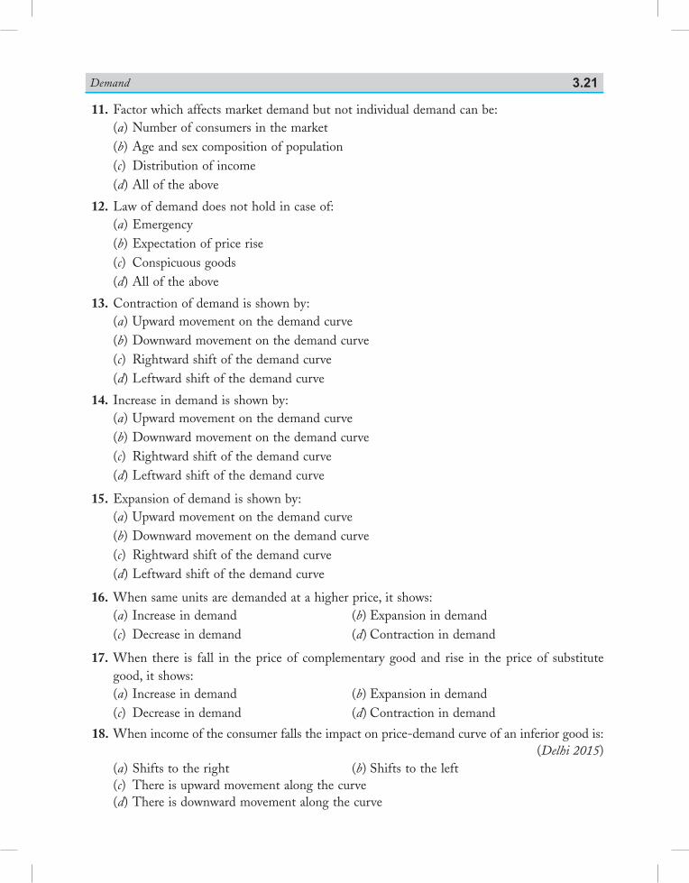
Demand 3.21
11. Factor which affects market demand but not individual demand can be: (a) Number of consumers in the market (b) Age and sex composition of population (c) Distribution of income (d) All of the above
12. Law of demand does not hold in case of: (a) Emergency (b) Expectation of price rise (c) Conspicuous goods (d) All of the above
13. Contraction of demand is shown by: (a) Upward movement on the demand curve (b) Downward movement on the demand curve (c) Rightward shift of the demand curve (d) Leftward shift of the demand curve
14. Increase in demand is shown by: (a) Upward movement on the demand curve (b) Downward movement on the demand curve (c) Rightward shift of the demand curve (d) Leftward shift of the demand curve
15. Expansion of demand is shown by: (a) Upward movement on the demand curve (b) Downward movement on the demand curve (c) Rightward shift of the demand curve (d) Leftward shift of the demand curve
16. When same units are demanded at a higher price, it shows: (a) Increase in demand (b) Expansion in demand (c) Decrease in demand (d) Contraction in demand
17. When there is fall in the price of complementary good and rise in the price of substitute good, it shows:
(a) Increase in demand (b) Expansion in demand (c) Decrease in demand (d) Contraction in demand
18. When income of the consumer falls the impact on price-demand curve of an inferior good is: (Delhi 2015)
(a) Shifts to the right (b) Shifts to the left (c) There is upward movement along the curve (d) There is downward movement along the curve
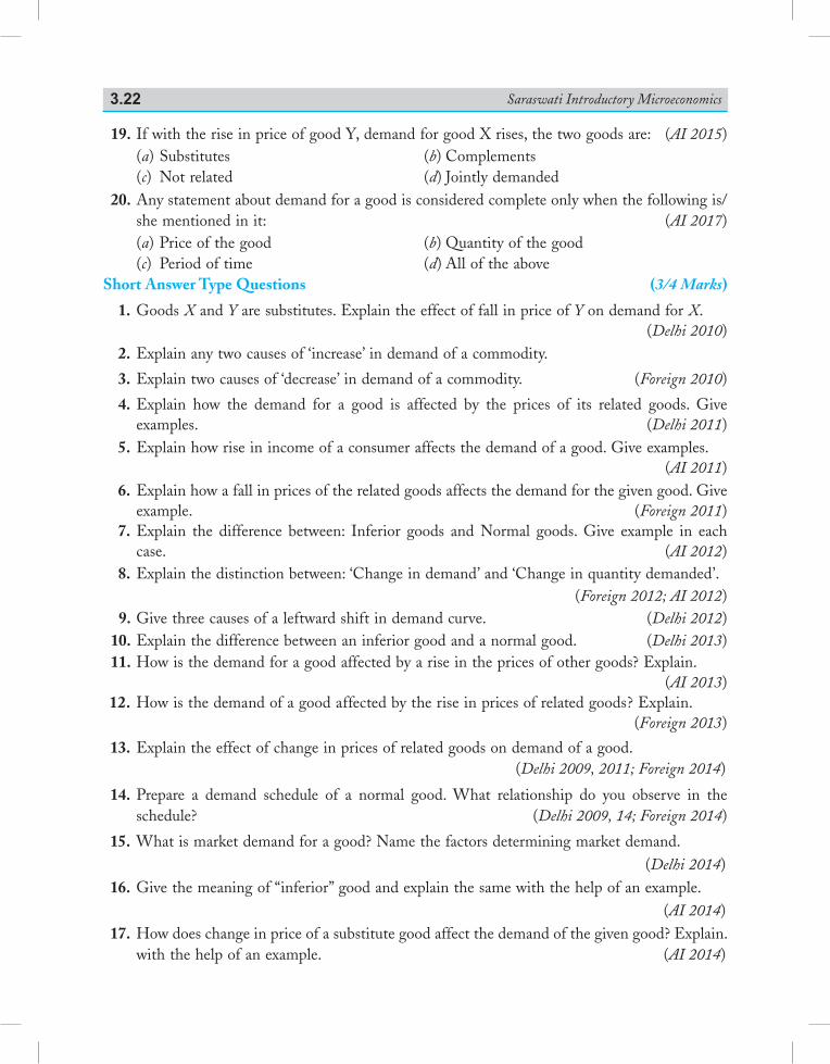
Saraswati Introductory Microeconomics3.22
19. If with the rise in price of good Y, demand for good X rises, the two goods are: (AI 2015) (a) Substitutes (b) Complements (c) Not related (d) Jointly demanded 20. Any statement about demand for a good is considered complete only when the following is/
she mentioned in it: (AI 2017) (a) Price of the good (b) Quantity of the good (c) Period of time (d) All of the aboveShort Answer Type Questions (3/4 Marks)
1. Goods X and Y are substitutes. Explain the effect of fall in price of Y on demand for X. (Delhi 2010) 2. Explain any two causes of ‘increase’ in demand of a commodity.
3. Explain two causes of ‘decrease’ in demand of a commodity. (Foreign 2010)
4. Explain how the demand for a good is affected by the prices of its related goods. Give examples. (Delhi 2011)
5. Explain how rise in income of a consumer affects the demand of a good. Give examples. (AI 2011) 6. Explain how a fall in prices of the related goods affects the demand for the given good. Give
example. (Foreign 2011) 7. Explain the difference between: Inferior goods and Normal goods. Give example in each
case. (AI 2012) 8. Explain the distinction between: ‘Change in demand’ and ‘Change in quantity demanded’. (Foreign 2012; AI 2012) 9. Give three causes of a leftward shift in demand curve. (Delhi 2012) 10. Explain the difference between an inferior good and a normal good. (Delhi 2013) 11. How is the demand for a good affected by a rise in the prices of other goods? Explain. (AI 2013) 12. How is the demand of a good affected by the rise in prices of related goods? Explain. (Foreign 2013)
13. Explain the effect of change in prices of related goods on demand of a good. (Delhi 2009, 2011; Foreign 2014)
14. Prepare a demand schedule of a normal good. What relationship do you observe in the schedule? (Delhi 2009, 14; Foreign 2014)
15. What is market demand for a good? Name the factors determining market demand. (Delhi 2014) 16. Give the meaning of “inferior” good and explain the same with the help of an example. (AI 2014) 17. How does change in price of a substitute good affect the demand of the given good? Explain.
with the help of an example. (AI 2014)
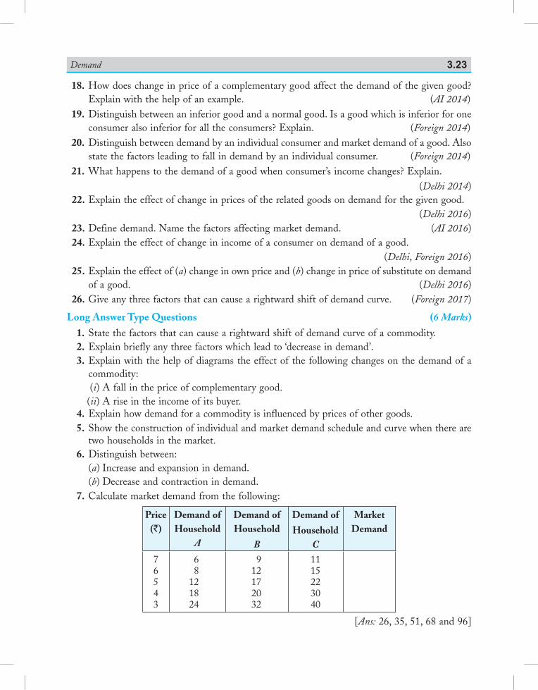
Demand 3.23
18. How does change in price of a complementary good affect the demand of the given good? Explain with the help of an example. (AI 2014)
19. Distinguish between an inferior good and a normal good. Is a good which is inferior for one consumer also inferior for all the consumers? Explain. (Foreign 2014)
20. Distinguish between demand by an individual consumer and market demand of a good. Also state the factors leading to fall in demand by an individual consumer. (Foreign 2014)
21. What happens to the demand of a good when consumer’s income changes? Explain.(Delhi 2014)
22. Explain the effect of change in prices of the related goods on demand for the given good. (Delhi 2016) 23. Define demand. Name the factors affecting market demand. (AI 2016) 24. Explain the effect of change in income of a consumer on demand of a good. (Delhi, Foreign 2016) 25. Explain the effect of (a) change in own price and (b) change in price of substitute on demand
of a good. (Delhi 2016) 26. Give any three factors that can cause a rightward shift of demand curve. (Foreign 2017)
Long Answer Type Questions (6 Marks)
1. State the factors that can cause a rightward shift of demand curve of a commodity. 2. Explain briefly any three factors which lead to ‘decrease in demand’. 3. Explain with the help of diagrams the effect of the following changes on the demand of a
commodity: (i) A fall in the price of complementary good. (ii) A rise in the income of its buyer. 4. Explain how demand for a commodity is influenced by prices of other goods. 5. Show the construction of individual and market demand schedule and curve when there are
two households in the market. 6. Distinguish between:
(a) Increase and expansion in demand.(b) Decrease and contraction in demand.
7. Calculate market demand from the following:
Price (`)
Demand of Household
A
Demand of Household
B
Demand of
Household C
Market Demand
76543
68
121824
912172032
1115223040
[Ans: 26, 35, 51, 68 and 96]
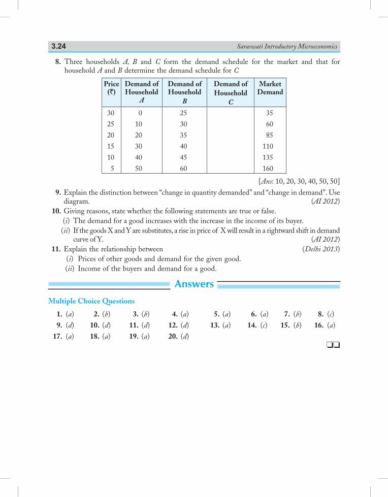
Saraswati Introductory Microeconomics3.24
8. Three households A, B and C form the demand schedule for the market and that for household A and B determine the demand schedule for C
Price (`)
Demand of Household
A
Demand of Household
B
Demand of Household
C
Market Demand
30
25
20
15
10
5
0
10
20
30
40
50
25
30
35
40
45
60
35
60
85
110
135
160
[Ans: 10, 20, 30, 40, 50, 50]
9. Explain the distinction between “change in quantity demanded” and “change in demand”. Use diagram. (AI 2012)
10. Giving reasons, state whether the following statements are true or false. (i) The demand for a good increases with the increase in the income of its buyer. (ii) If the goods X and Y are substitutes, a rise in price of X will result in a rightward shift in demand
curve of Y. (AI 2012) 11. Explain the relationship between (Delhi 2013) (i) Prices of other goods and demand for the given good. (ii) Income of the buyers and demand for a good.
AnswersMultiple Choice Questions
1. (a) 2. (b) 3. (b) 4. (a) 5. (a) 6. (a) 7. (b) 8. (c) 9. (d) 10. (d) 11. (d) 12. (d) 13. (a) 14. (c) 15. (b) 16. (a) 17. (a) 18. (a) 19. (a) 20. (d)
4Elasticity of Demand
Chapter Scheme
4.1 Definition of Price elasticity of DemanD
The law of demand states that when the price of a good falls, consumers demand more units of the good. But how much more? It is important and useful to have magnitude of change in quantity demanded to a change in price. It is called price elasticity of demand.
Price elasticity of demand measures the responsiveness of demand of a good to a change in its price. Alfred Marshall was the first economist to formulate the concept of price elasticity of demand as the ratio of a relative change in quantity demanded to a relative change in price. A relative measure is needed so that changes in different measures can be compared. These relative changes in demand and price are measured by percentage changes. The percentage changes are independent of units. Numerically, price elasticity of demand eD, is calculated as:
eD = – percentage change in quantity demandedpercentage change in price
eD = –
change in quantity demandedoriginal quantity demanded
change in priiceoriginal price
= – ( ) /( ) /Q Q QP P P
1
1
−−
= −
∆
∆
QQP
P
= − ∆∆
QP
PQ
.
4.1 Definition of Price Elasticity of Demand
4.2 Factors Affecting Price Elasticity of Demand
4.3 Measurement of Price Elasticity of Demand by Percentage Method
Solved Numerical Problems Points to Remember Test Your Knowledge Answers to MCQs
Saraswati Introductory Microeconomics4.2
where,
DQ = Change in quantity demanded (or Q1 – Q) Q = Original quantity demanded DP = Change in price (or P1 – P)
P = Original price
eD = Coefficient of elasticity of demand. eD is negative. The ratio is a negative number because price and quantity demanded are inversely related. In numerical sums, the minus sign is dropped from the numbers and all percentage changes are treated as positive.
4.2 factors affecting Price elasticity of DemanD
The factors which determine the price elasticity of demand for a commodity or service are:1. Availability of Close Substitute. A good having close substitutes will have an elastic demand
and a good with no close substitutes will have an inelastic demand. Example: commodities such as pen, cold drink, car, etc. have close substitutes. When the price of these goods rise, the price of their substitutes remaining constant, there is proportionately greater fall in the quantity demanded of these goods. That is, their demand is elastic. Commodities such as prescribed medicines and salt have no close substitutes and hence, have an inelastic demand.
2. Income of the Consumers. If the income level of consumers is high, the elasticity of demand is less. It is because change in the price will not affect the quantity demanded by a greater proportion. But in low income groups, the elasticity of demand is high.
3. Luxuries versus Necessities. The price elasticity of demand is likely to be low for necessities and high for luxuries. A necessity is a good or service that the consumer must have such as food (bread, milk) and medicines. Luxuries are goods that are enjoyable but not essential. Example: eating in a 5-Star hotel. If the price of necessities rise, then demand will not fall by a greater proportion because their purchase cannot be delayed. That is why, the price elasticity of demand in case of necessity is low.
4. Proportion of Total Expenditure Spent on the Product. Higher the cost of the good relative to total income of the consumer, more will be the price elasticity of demand. If the price of bread, ink, salt, match box, etc., which is relatively low, doubles it would have almost no effect on the quantity demanded of them. On the other hand, if price of car doubles then the quantity demanded will fall by a greater proportion showing high price elasticity of demand.
5. Number of Uses of the Commodity. The more the number of uses a commodity can be put to, the more elastic is the demand. If a commodity has few uses, it has an inelastic demand. Examples: goods like milk, eggs and electricity can be put to many different uses and hence, enjoy elastic demand, i.e., when prices are low, demand increases by a greater proportion as the goods can now be put to less important uses also.
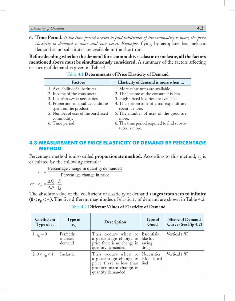
Elasticity of Demand 4.3
6. Time Period. If the time period needed to find substitutes of the commodity is more, the price elasticity of demand is more and vice versa. Example: flying by aeroplane has inelastic demand as no substitutes are available in the short run.
Before deciding whether the demand for a commodity is elastic or inelastic, all the factors mentioned above must be simultaneously considered. A summary of the factors affecting elasticity of demand is given in Table 4.1.
Table 4.1 Determinants of Price Elasticity of Demand
Factors Elasticity of demand is more when....
1. Availability of substitutes.2. Income of the consumers.3. Luxuries versus necessities.4. Proportion of total expenditure
spent on the product.5. Number of uses of the purchased
commodity.6. Time period.
1. More substitutes are available.2. The income of the consumer is less.3. High priced luxuries are available.4. The proportion of total expenditure
spent is more.5. The number of uses of the good are
more.6. The time period required to find substi-
tutes is more.
4.3 measurement of Price elasticity of DemanD by Percentage methoD
Percentage method is also called proportionate method. According to this method, eD is calculated by the following formula:
eD =
or eD = ∆∆
QP
PQ
⋅
The absolute value of the coefficient of elasticity of demand ranges from zero to infinity (0 < eD < ∞). The five different magnitudes of elasticity of demand are shown in Table 4.2.
Table 4.2 Different Values of Elasticity of Demand
Coefficient Type of eD
Type of eD
Description Type of Good
Shape of Demand Curve (See Fig 4.2)
1. eD = 0 Perfectlyinelasticdemand
This occurs when to a percentage change in price there is no change in quantity demanded.
Essentialslike lifesavingdrugs
Vertical (dF)
2. 0 < eD < 1 Inelastic This occurs when to a percentage change in price there is less than proportionate change in quantity demanded.
Necessitiesl i ke food , fuel
Vertical (dF)
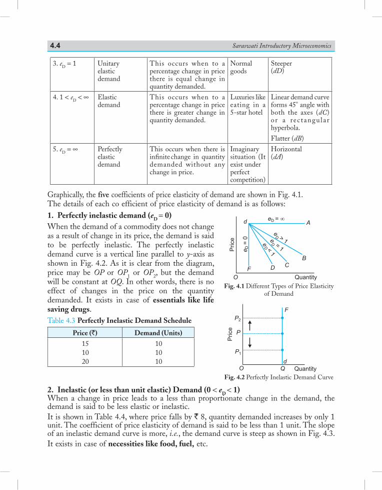
Saraswati Introductory Microeconomics4.4
3. eD = 1 Unitaryelasticdemand
This occurs when to a percentage change in price there is equal change in quantity demanded.
Normalgoods
Steeper(dD)
4. 1 < eD < ∞ Elasticdemand
This occurs when to a percentage change in price there is greater change in quantity demanded.
Luxuries like eating in a 5-star hotel
Linear demand curve forms 45° angle with both the axes (dC) o r a rec tangu la r hyperbola.
Flatter (dB)
5. eD = ∞ Perfectlyelasticdemand
This occurs when there is infinite change in quantity demanded without any change in price.
Imaginarysituation (It exist underperfectcompetition)
Horizontal(dA)
Graphically, the five coefficients of price elasticity of demand are shown in Fig. 4.1.The details of each co efficient of price elasticity of demand is as follows:1. Perfectly inelastic demand (eD = 0)When the demand of a commodity does not change as a result of change in its price, the demand is said to be perfectly inelastic. The perfectly inelastic demand curve is a vertical line parallel to y-axis as shown in Fig. 4.2. As it is clear from the diagram, price may be OP or OP1 or OP2, but the demand will be constant at OQ. In other words, there is no effect of changes in the price on the quantity demanded. It exists in case of essentials like life saving drugs.Table 4.3 Perfectly Inelastic Demand Schedule
Price (`) Demand (Units)
151020
101010
2. Inelastic (or less than unit elastic) Demand (0 < eD < 1)When a change in price leads to a less than proportionate change in the demand, the demand is said to be less elastic or inelastic.It is shown in Table 4.4, where price falls by ` 8, quantity demanded increases by only 1 unit. The coefficient of price elasticity of demand is said to be less than 1 unit. The slope of an inelastic demand curve is more, i.e., the demand curve is steep as shown in Fig. 4.3.It exists in case of necessities like food, fuel, etc.
Fig. 4.1 Different Types of Price Elasticity of Demand
Fig. 4.2 Perfectly Inelastic Demand Curve
Pric
e
P2
P
P1
F
dO Q Quantity
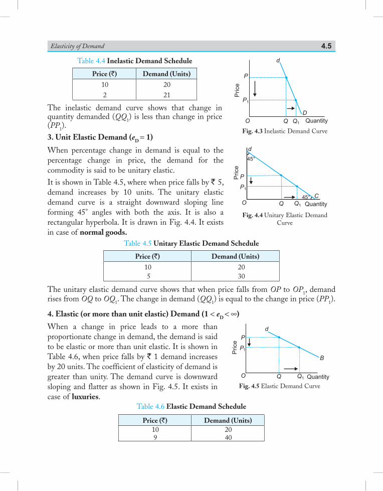
Elasticity of Demand 4.5
Table 4.4 Inelastic Demand Schedule
Price (`) Demand (Units)
102
2021
The inelastic demand curve shows that change in quantity demanded (QQ1) is less than change in price (PP1).3. Unit Elastic Demand (eD = 1)
When percentage change in demand is equal to the percentage change in price, the demand for the commodity is said to be unitary elastic.It is shown in Table 4.5, where when price falls by ` 5, demand increases by 10 units. The unitary elastic demand curve is a straight downward sloping line forming 45° angles with both the axis. It is also a rectangular hyperbola. It is drawn in Fig. 4.4. It exists in case of normal goods.
Table 4.5 Unitary Elastic Demand Schedule
Price (`) Demand (Units)
10 5
2030
The unitary elastic demand curve shows that when price falls from OP to OP1, demand rises from OQ to OQ1. The change in demand (QQ1) is equal to the change in price (PP1).
4. Elastic (or more than unit elastic) Demand (1 < eD < ∞)
When a change in price leads to a more than proportionate change in demand, the demand is said to be elastic or more than unit elastic. It is shown in Table 4.6, when price falls by ` 1 demand increases by 20 units. The coefficient of elasticity of demand is greater than unity. The demand curve is downward sloping and flatter as shown in Fig. 4.5. It exists in case of luxuries.
Table 4.6 Elastic Demand Schedule
Price (`) Demand (Units)109
2040
Quantity
D
QO
P
P1
d
Price
Q1
Fig. 4.3 Inelastic Demand Curve
Pric
e
P
P1
O Q Q1 Quantity45°
45°
C
d
Fig. 4.4 Unitary Elastic Demand Curve
Price
d
B
P
P1
O Q Q1 Quantity
Fig. 4.5 Elastic Demand Curve
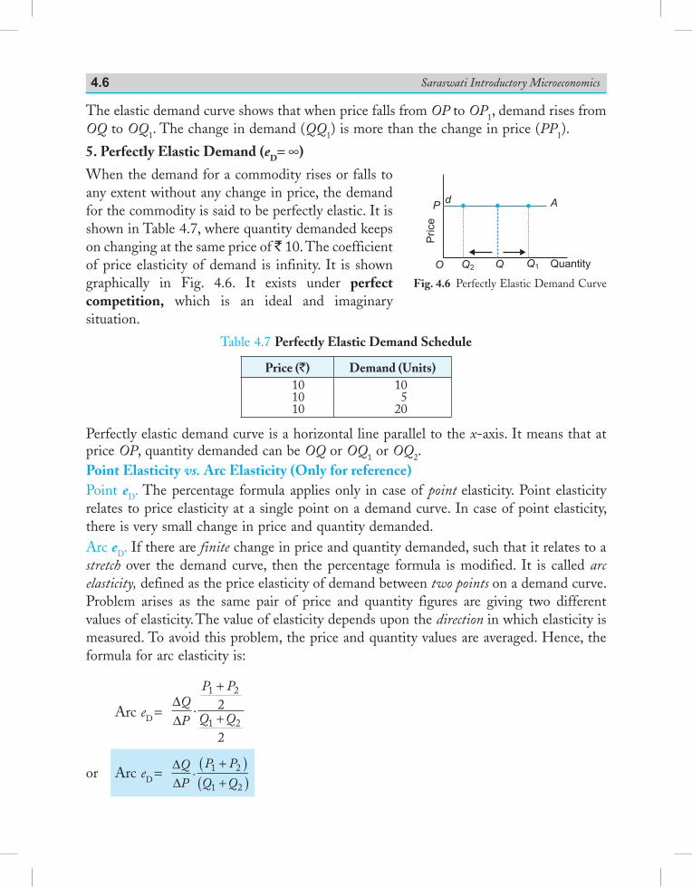
Saraswati Introductory Microeconomics4.6
The elastic demand curve shows that when price falls from OP to OP1, demand rises from OQ to OQ1. The change in demand (QQ1) is more than the change in price (PP1).
5. Perfectly Elastic Demand (eD= ∞)
When the demand for a commodity rises or falls to any extent without any change in price, the demand for the commodity is said to be perfectly elastic. It is shown in Table 4.7, where quantity demanded keeps on changing at the same price of ` 10. The coefficient of price elasticity of demand is infinity. It is shown graphically in Fig. 4.6. It exists under perfect competition, which is an ideal and imaginary situation.
Table 4.7 Perfectly Elastic Demand Schedule
Price (`) Demand (Units)101010
105
20
Perfectly elastic demand curve is a horizontal line parallel to the x-axis. It means that at price OP, quantity demanded can be OQ or OQ1 or OQ2.Point Elasticity vs. Arc Elasticity (Only for reference)Point eD. The percentage formula applies only in case of point elasticity. Point elasticity relates to price elasticity at a single point on a demand curve. In case of point elasticity, there is very small change in price and quantity demanded.Arc eD. If there are finite change in price and quantity demanded, such that it relates to a stretch over the demand curve, then the percentage formula is modified. It is called arc elasticity, defined as the price elasticity of demand between two points on a demand curve. Problem arises as the same pair of price and quantity figures are giving two different values of elasticity. The value of elasticity depends upon the direction in which elasticity is measured. To avoid this problem, the price and quantity values are averaged. Hence, the formula for arc elasticity is:
Arc eD = ∆∆
QP
P P
Q Q.
1 2
1 2
2
2
+
+
or Arc eD = ∆∆
QP
P P
Q Q. 1 2
1 2
+( )+( )
Pric
e
P d
O Q2 Q Q1 Quantity
A
Fig. 4.6 Perfectly Elastic Demand Curve
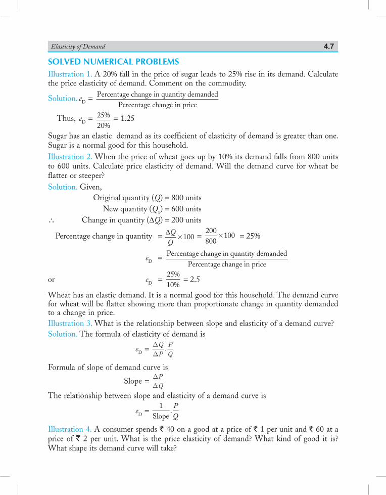
Elasticity of Demand 4.7
Solved Numerical ProblemSIllustration 1. A 20% fall in the price of sugar leads to 25% rise in its demand. Calculate the price elasticity of demand. Comment on the commodity.
Solution. eD = Percentage change in quantity demandedPercentage change in price
Thus, eD = 25%20%
= 1.25
Sugar has an elastic demand as its coefficient of elasticity of demand is greater than one. Sugar is a normal good for this household.Illustration 2. When the price of wheat goes up by 10% its demand falls from 800 units to 600 units. Calculate price elasticity of demand. Will the demand curve for wheat be flatter or steeper?Solution. Given,
Original quantity (Q) = 800 units New quantity (Q1) = 600 units
\ Change in quantity (DQ) = 200 units
Percentage change in quantity = ∆QQ
× 100 = 200800
100× = 25%
eD = Percentage change in quantity demandedPercentage change in price
or eD = 2510
%%
= 2.5
Wheat has an elastic demand. It is a normal good for this household. The demand curve for wheat will be flatter showing more than proportionate change in quantity demanded to a change in price.Illustration 3. What is the relationship between slope and elasticity of a demand curve?Solution. The formula of elasticity of demand is
eD = DDQPPQ
.
Formula of slope of demand curve is
Slope = DDPQ
The relationship between slope and elasticity of a demand curve is
eD = 1
Slope.PQ
Illustration 4. A consumer spends ` 40 on a good at a price of ` 1 per unit and ` 60 at a price of ` 2 per unit. What is the price elasticity of demand? What kind of good it is? What shape its demand curve will take?
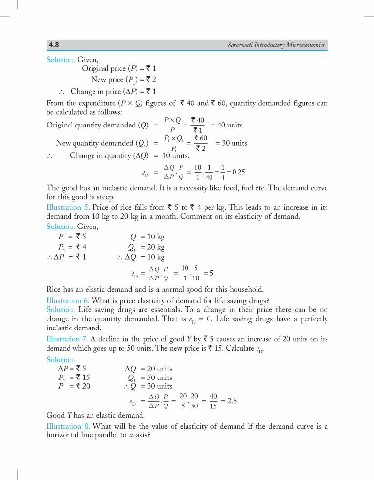
Saraswati Introductory Microeconomics4.8
Solution. Given, Original price (P) = ` 1 New price (P1) = ` 2\ Change in price (DP) = ` 1
From the expenditure (P × Q) figures of ` 40 and ` 60, quantity demanded figures can be calculated as follows:
Original quantity demanded (Q) = P Q
P×
= ``401
= 40 units
New quantity demanded (Q1) = P Q
P1 1
1
× =
``602
= 30 units
\ Change in quantity (DQ) = 10 units.
eD = DDQPPQ
. = 101
. .1
4014
0 25= =
The good has an inelastic demand. It is a necessity like food, fuel etc. The demand curve for this good is steep.Illustration 5. Price of rice falls from ` 5 to ` 4 per kg. This leads to an increase in its demand from 10 kg to 20 kg in a month. Comment on its elasticity of demand.Solution. Given,
P = ` 5 Q = 10 kgP1 = ` 4 Q1 = 20 kg
\ DP = ` 1 \ DQ = 10 kg
eD = DDQPPQ
. = 101
510
. = 5
Rice has an elastic demand and is a normal good for this household.Illustration 6. What is price elasticity of demand for life saving drugs?Solution. Life saving drugs are essentials. To a change in their price there can be no change in the quantity demanded. That is eD = 0. Life saving drugs have a perfectly inelastic demand.Illustration 7. A decline in the price of good Y by ` 5 causes an increase of 20 units on its demand which goes up to 50 units. The new price is ` 15. Calculate eD.Solution.
DP = ` 5 DQ = 20 unitsP1 = ` 15 Q1 = 50 unitsP = ` 20 \Q = 30 units
eD = DDQPPQ
. = 205
2030
. = 4015
= 2.6
Good Y has an elastic demand.Illustration 8. What will be the value of elasticity of demand if the demand curve is a horizontal line parallel to x-axis?
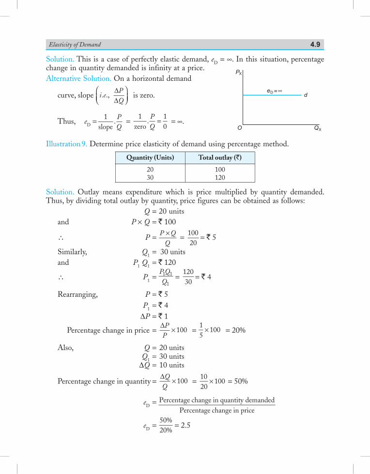
Elasticity of Demand 4.9
Solution. This is a case of perfectly elastic demand, eD = ∞. In this situation, percentage change in quantity demanded is infinity at a price.Alternative Solution. On a horizontal demand
curve, slope i ePQ
. ., ∆∆
is zero.
Thus, eD = 1slope
.PQ
= 1
zero.
10
PQ
= = ∞.
Illustration 9. Determine price elasticity of demand using percentage method.
Quantity (Units) Total outlay (`)
2030
100120
Solution. Outlay means expenditure which is price multiplied by quantity demanded. Thus, by dividing total outlay by quantity, price figures can be obtained as follows: Q = 20 units
and P × Q = ` 100
\ P = P QQ× =
10020
= ` 5
Similarly, Q1 = 30 unitsand P1 Q1 = ` 120
\ P1 = P QQ1 1
1 =
12030
= ` 4
Rearranging, P = ` 5 P1 = ` 4 DP = ` 1
Percentage change in price = ∆PP
× 100 = 15
100× = 20%
Also, Q = 20 units Q1 = 30 units DQ = 10 units
Percentage change in quantity = ∆QQ
× 100 = 1020
100× = 50%
eD = Percentage change in quantity demandedPercentage change in price
eD = 5020
%%
= 2.5
QX
PX
de =D ∞
O
Saraswati Introductory Microeconomics4.10
Illustration 10. The price elasticity is 0.5. The % change in quantity is 4. What is the % change in price?Solution.
eD = 0.5 % change in quantity = 4
% change in price = % change in quantity
De= =4
0 58
.
Illustration 11. The price of cauliflower goes up by 8% and the total expenditure by a family on cauliflower goes up by 5%. What can we say about the elasticity of demand for cauliflower by this family?Solution. Since with rise in price, total expenditure also rises, it is a case of inelastic demand (eD < 1).Illustration 12. A dentist was charging ` 300 for a standard cleaning job and per month it used to generate total revenue equal to ` 30,000. She has since last month increased the price of dental cleaning to ` 350. As a result, fewer customers are now coming for dental cleaning, but the total revenue is now ` 33,250. From this, what can we conclude about the elasticity of demand for such a dental service?Solution. Given, P = ` 300, Total revenue (P × Q) = ` 30,000 P1 = ` 350, Total revenue (P1 × Q1) = ` 33,250
Therefore, when P = ` 300, QP Q
P= × = =30 000
300100
,
and when P1 = ` 350, Q P QP1
1 1
1
33 250350
95= × = =,
\ eD = = 300100
= 3
10 = 0.3
∆∆
QP
PQ
× ×550
Thus, demand for dental service is inelastic since eD is less than one.Illustration 13. Price of good X rises from ` 20 to ` 30 per unit. Consequently, its demand falls by 20 units and becomes 100 units. Determine price elasticity of demand.Solution. Given,
P = ` 20 DQ = 20 units
P1 = ` 30 Q1 = 100 units
DP = ` 10 \ Q = 120 units
\ eD = ∆∆
⋅QP
PQ
= 2010
20120
13
⋅ = = 0.33
Illustration 14. Originally, a product was sold for ` 10 and the quantity demanded was 1,000 units. The product price changes to ` 14 and as a result the quantity demanded changes to 500 units. Calculate the price elasticity.
Elasticity of Demand 4.11
Solution. P = ` 10 Q = 1,000 units P1 = ` 14 Q1 = 500 units
\ eD = ∆∆
⋅ = ×QP
PQ
5004
101000
= 54
1 25= .
Illustration 15. Which of the following commodities have inelastic demand? Salt, a particular brand of lipstick, medicine, mobile phone and school uniform.Solution. Salt, medicine, school uniform have inelastic demand as they do not have many substitutes. On the other hand, mobile phone and a particular brand of lipstick has an elastic demand since they have many substitutes.Illustration 16. The price elasticity is 2. The % change in price is equal to 5. Find the % change in quantity.Solution. eD = 2 % change in P = 5
Since eD =% change in quantity
% change in price\ % change in quantity = eD × % change in price = 2 × 5 = 10
Illustration 17. Let the demand function be: Q = 10 – 2P. Find eD at a price of 5/2.
Solution. Q = 10 – 2P. Differentiating Q with respect to P, we get DDQP
= – 2
Also, when P = 5/2, Q = 10 – 252
⋅ = 5
\ eD = –QP
.PQ
DD
= –/
–25 2
52
52
15
× = × × = |–1| = 1.
Illustration 18. Let eD = –0.4. By what percentage the quantity demanded goes down if price of the good increases by 4%?
Solution. eD = % change in quantity demanded% change in price
|–0.4| = % change in quantity demanded
4 0.4 × 4 = 1.6
\ % fall in quantity demanded is 0.4 × 4 = 1.6%
Illustration 19. Let slope of demand curve = – 0.5. Calculate eD when initial price is ` 20 per unit and initial quantity is 50 units of the commodity.
Saraswati Introductory Microeconomics4.12
Solution. Slope of demand curve = DDPQ
= – 0.5
\ 1
Slope= ∆
∆=Q
P–
.1
0 5
eD = –QP
.PQ
DD
= –.1
0 52050
⋅ = |–0.8| = 0.8
Illustration 20. A consumer spends ` 80 on a commodity at a price of ` 1 per unit and ` 100 at a price of ` 2 per unit. What is the price elasticity of demand?
Solution. When P = 1, PQ = 80 ⇒ Q = 801
80=
When P1 = 2, P1Q1 = 100 ⇒ Q1 =100
250=
eD = DD
QP
PQ
. = 301
180
0 38. .=
Illustration 21. When the price of a commodity falls by ̀ 2 per unit, its quantity demanded increases by 10 units. Its price elasticity of demand is (–)1. Calculate its quantity demanded at the price before change which was ` 10 per unit.
Solution. DP = 2, DQ = 10 eD = – 1 P = 10 Q = ? eD = ∆
∆QP
PQ
×
⇒ 1 = 102
10×
Q
⇒ Q = 50 units
Illustration 22. When price of a commodity falls by ` 1 per unit, its quantity demanded rises by 3 units. Its price elasticity of demand is (–)2. Calculate its quantity demanded if the price before the change was ` 10 per unit.
Solution. DP = 1 DQ = 3 eD = – 2 P = 10 Q = ? \ P1 = 9
\ eD = ∆∆
QP
PQ
×
2 = 31
10×
Q
⇒ Q = 15 units
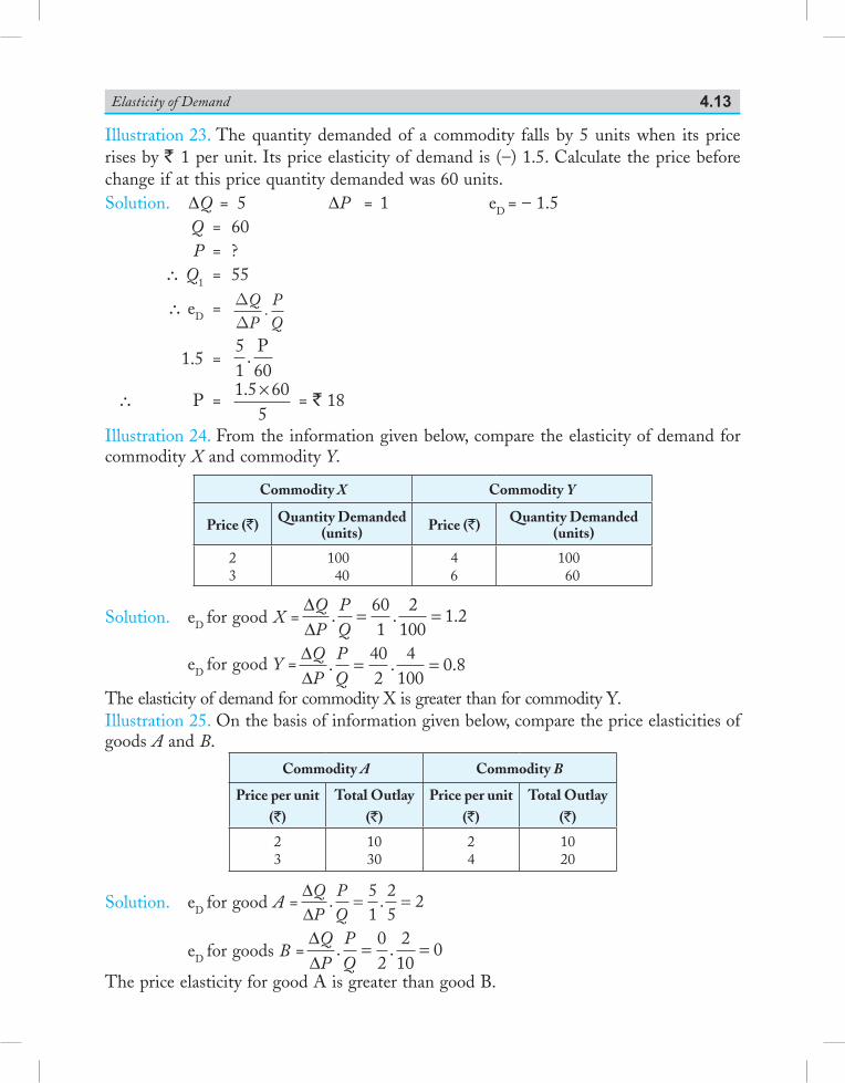
Elasticity of Demand 4.13
Illustration 23. The quantity demanded of a commodity falls by 5 units when its price rises by ` 1 per unit. Its price elasticity of demand is (–) 1.5. Calculate the price before change if at this price quantity demanded was 60 units.Solution. DQ = 5 DP = 1 eD = – 1.5 Q = 60 P = ? \ Q1 = 55
\ eD = DD
QP
PQ
.
1.5 = 51 60
.P
\ P = 1 5 60
5. ×
= ` 18
Illustration 24. From the information given below, compare the elasticity of demand for commodity X and commodity Y.
Commodity X Commodity Y
Price (`) Quantity Demanded (units) Price (`) Quantity Demanded
(units)
23
10040
46
10060
Solution. eD for good X =∆∆
QP
PQ
. . .= =601
2100
1 2
eD for good Y =∆∆
QP
PQ
. . .= =402
4100
0 8
The elasticity of demand for commodity X is greater than for commodity Y.Illustration 25. On the basis of information given below, compare the price elasticities of goods A and B.
Commodity A Commodity B
Price per unit (`)
Total Outlay (`)
Price per unit (`)
Total Outlay (`)
23
1030
24
1020
Solution. eD for good A =∆∆
QP
PQ
. .= =51
25
2
eD for goods B =∆∆
QP
PQ
. .= =02
210
0
The price elasticity for good A is greater than good B.
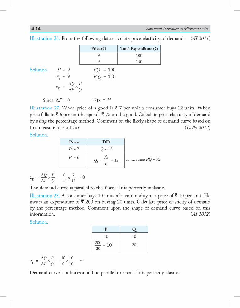
Saraswati Introductory Microeconomics4.14
Illustration 26. From the following data calculate price elasticity of demand: (AI 2011)
Price (`) Total Expenditure (`)
99
100150
Solution. P = 9 PQ = 100 P1 = 9 P1Q1 = 150
eD = ∆∆
QP
PQ
×
Since ∆P = 0 ∴ ∞e =D
Illustration 27. When price of a good is ` 7 per unit a consumer buys 12 units. When price falls to ` 6 per unit he spends ` 72 on the good. Calculate price elasticity of demand by using the percentage method. Comment on the likely shape of demand curve based on this measure of elasticity. (Delhi 2012)Solution.
Price DD
P = 7 Q = 12
P1 = 6Q1 =
726
= 12 ........ since PQ = 72
eD = ∆∆
QP
PQ
× = 01
712−
× = 0
The demand curve is parallel to the Y-axis. It is perfectly inelastic.
Illustration 28. A consumer buys 10 units of a commodity at a price of ` 10 per unit. He incurs an expenditure of ` 200 on buying 20 units. Calculate price elasticity of demand by the percentage method. Comment upon the shape of demand curve based on this information. (AI 2012)
Solution.P Q
10 1020020
= 10 20
eD = ∆∆
QP
PQ
× = × = ∞100
1010
Demand curve is a horizontal line parallel to x-axis. It is perfectly elastic.
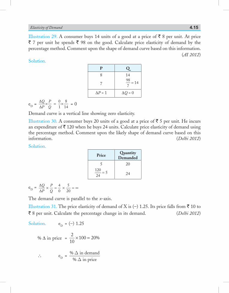
Elasticity of Demand 4.15
Illustration 29. A consumer buys 14 units of a good at a price of ` 8 per unit. At price ` 7 per unit he spends ` 98 on the good. Calculate price elasticity of demand by the percentage method. Comment upon the shape of demand curve based on this information. (AI 2012)Solution.
P Q
8
7
14 98
714=
DP = 1 DQ = 0
eD = ∆∆
QP
PQ
× = ×01
814
= 0
Demand curve is a vertical line showing zero elasticity.
Illustration 30. A consumer buys 20 units of a good at a price of ` 5 per unit. He incurs an expenditure of ` 120 when he buys 24 units. Calculate price elasticity of demand using the percentage method. Comment upon the likely shape of demand curve based on this information. (Delhi 2012)
Solution.
Price Quantity Demanded
5 2012024
5= 24
eD = ∆∆
QP
PQ
× = × = ∞40
520
The demand curve is parallel to the x-axis.
Illustration 31. The price elasticity of demand of X is (–) 1.25. Its price falls from ` 10 to ` 8 per unit. Calculate the percentage change in its demand. (Delhi 2012)
Solution. eD = (–) 1.25
% D in price = 2
10100 20× = %
\ eD = % in demand% in priceDD
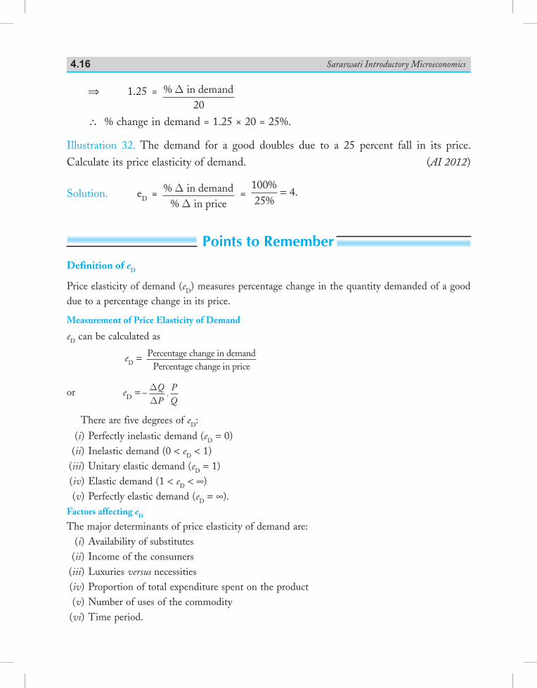
Saraswati Introductory Microeconomics4.16
⇒ 1.25 = % in demand20
D
\ % change in demand = 1.25 × 20 = 25%.
Illustration 32. The demand for a good doubles due to a 25 percent fall in its price. Calculate its price elasticity of demand. (AI 2012)
Solution. eD = % in demand% in priceDD
= 10025
4%%
.=
Points to rememberDefinition of eD
Price elasticity of demand (eD) measures percentage change in the quantity demanded of a good due to a percentage change in its price.
Measurement of Price Elasticity of Demand
eD can be calculated as
eD = Percentage change in demandPercentage change in price
or eD = –QP
.PQ
DD
There are five degrees of eD:
(i) Perfectly inelastic demand (eD = 0) (ii) Inelastic demand (0 < eD < 1) (iii) Unitary elastic demand (eD = 1) (iv) Elastic demand (1 < eD < ∞) (v) Perfectly elastic demand (eD = ∞).Factors affecting eD
The major determinants of price elasticity of demand are: (i) Availability of substitutes (ii) Income of the consumers (iii) Luxuries versus necessities (iv) Proportion of total expenditure spent on the product (v) Number of uses of the commodity (vi) Time period.
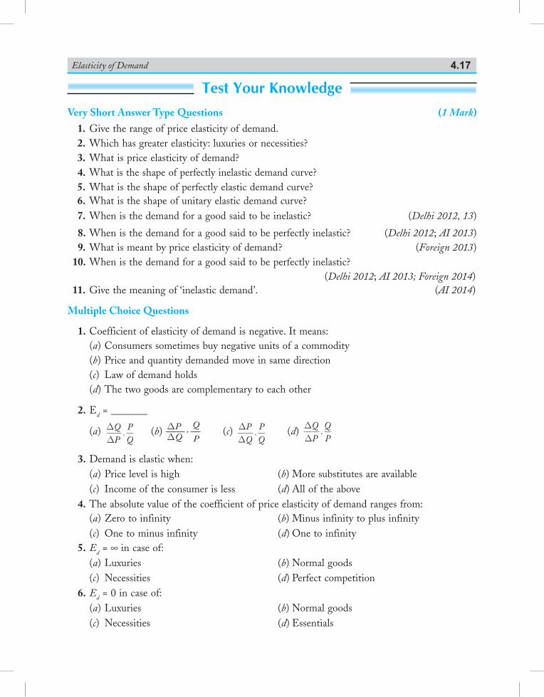
Elasticity of Demand 4.17
Test Your KnowledgeVery Short Answer Type Questions (1 Mark)
1. Give the range of price elasticity of demand. 2. Which has greater elasticity: luxuries or necessities? 3. What is price elasticity of demand? 4. What is the shape of perfectly inelastic demand curve? 5. What is the shape of perfectly elastic demand curve? 6. What is the shape of unitary elastic demand curve? 7. When is the demand for a good said to be inelastic? (Delhi 2012, 13)
8. When is the demand for a good said to be perfectly inelastic? (Delhi 2012; AI 2013) 9. What is meant by price elasticity of demand? (Foreign 2013) 10. When is the demand for a good said to be perfectly inelastic? (Delhi 2012; AI 2013; Foreign 2014) 11. Give the meaning of ‘inelastic demand’. (AI 2014)
Multiple Choice Questions
1. Coefficient of elasticity of demand is negative. It means: (a) Consumers sometimes buy negative units of a commodity (b) Price and quantity demanded move in same direction (c) Law of demand holds (d) The two goods are complementary to each other
2. Ed = _______
(a) DD
QP
PQ
. (b) DPDQ
Q
P (c) D
DPQ
PQ
. (d) DD
QP
QP
.
3. Demand is elastic when: (a) Price level is high (b) More substitutes are available (c) Income of the consumer is less (d) All of the above 4. The absolute value of the coefficient of price elasticity of demand ranges from: (a) Zero to infinity (b) Minus infinity to plus infinity (c) One to minus infinity (d) One to infinity 5. Ed = ∞ in case of: (a) Luxuries (b) Normal goods (c) Necessities (d) Perfect competition 6. Ed = 0 in case of: (a) Luxuries (b) Normal goods (c) Necessities (d) Essentials
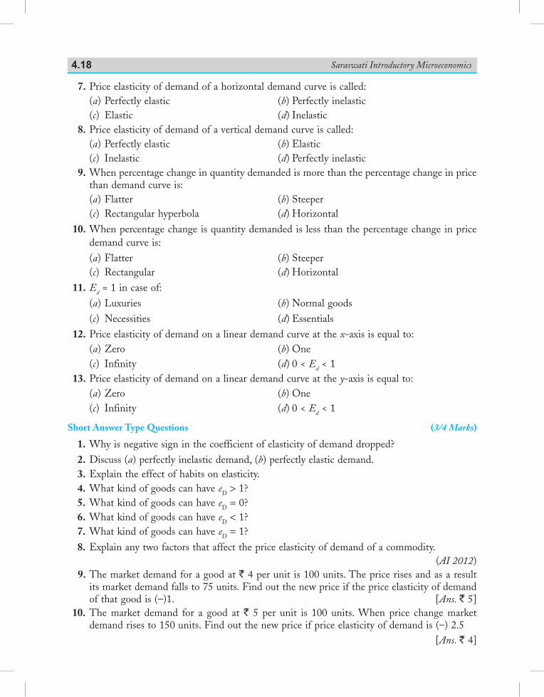
Saraswati Introductory Microeconomics4.18
7. Price elasticity of demand of a horizontal demand curve is called: (a) Perfectly elastic (b) Perfectly inelastic (c) Elastic (d) Inelastic 8. Price elasticity of demand of a vertical demand curve is called: (a) Perfectly elastic (b) Elastic (c) Inelastic (d) Perfectly inelastic 9. When percentage change in quantity demanded is more than the percentage change in price
than demand curve is: (a) Flatter (b) Steeper (c) Rectangular hyperbola (d) Horizontal 10. When percentage change is quantity demanded is less than the percentage change in price
demand curve is: (a) Flatter (b) Steeper (c) Rectangular (d) Horizontal 11. Ed = 1 in case of: (a) Luxuries (b) Normal goods (c) Necessities (d) Essentials 12. Price elasticity of demand on a linear demand curve at the x-axis is equal to: (a) Zero (b) One (c) Infinity (d) 0 < Ed < 1 13. Price elasticity of demand on a linear demand curve at the y-axis is equal to: (a) Zero (b) One (c) Infinity (d) 0 < Ed < 1
Short Answer Type Questions (3/4 Marks)
1. Why is negative sign in the coefficient of elasticity of demand dropped? 2. Discuss (a) perfectly inelastic demand, (b) perfectly elastic demand. 3. Explain the effect of habits on elasticity. 4. What kind of goods can have eD > 1? 5. What kind of goods can have eD = 0? 6. What kind of goods can have eD < 1? 7. What kind of goods can have eD = 1?
8. Explain any two factors that affect the price elasticity of demand of a commodity. (AI 2012) 9. The market demand for a good at ` 4 per unit is 100 units. The price rises and as a result
its market demand falls to 75 units. Find out the new price if the price elasticity of demand of that good is (–)1. [Ans. ` 5]
10. The market demand for a good at ` 5 per unit is 100 units. When price change market demand rises to 150 units. Find out the new price if price elasticity of demand is (–) 2.5
[Ans. ` 4]
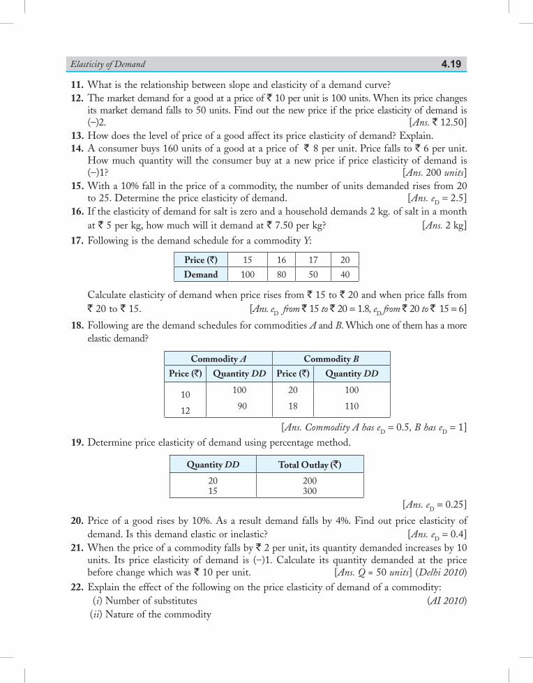
Elasticity of Demand 4.19
11. What is the relationship between slope and elasticity of a demand curve? 12. The market demand for a good at a price of ` 10 per unit is 100 units. When its price changes
its market demand falls to 50 units. Find out the new price if the price elasticity of demand is (–)2. [Ans. ` 12.50]
13. How does the level of price of a good affect its price elasticity of demand? Explain. 14. A consumer buys 160 units of a good at a price of ` 8 per unit. Price falls to ` 6 per unit.
How much quantity will the consumer buy at a new price if price elasticity of demand is (–)1? [Ans. 200 units]
15. With a 10% fall in the price of a commodity, the number of units demanded rises from 20 to 25. Determine the price elasticity of demand. [Ans. eD = 2.5]
16. If the elasticity of demand for salt is zero and a household demands 2 kg. of salt in a month at ` 5 per kg, how much will it demand at ` 7.50 per kg? [Ans. 2 kg]
17. Following is the demand schedule for a commodity Y:
Price (`) 15 16 17 20
Demand 100 80 50 40
Calculate elasticity of demand when price rises from ` 15 to ` 20 and when price falls from ` 20 to ` 15. [Ans. eD from ` 15 to ` 20 = 1.8, eD from ` 20 to ` 15 = 6]
18. Following are the demand schedules for commodities A and B. Which one of them has a more elastic demand?
Commodity A Commodity B
Price (`) Quantity DD Price (`) Quantity DD
10
12
100
90
20
18
100
110
[Ans. Commodity A has eD = 0.5, B has eD = 1] 19. Determine price elasticity of demand using percentage method.
Quantity DD Total Outlay (`)
2015
200300
[Ans. eD = 0.25]
20. Price of a good rises by 10%. As a result demand falls by 4%. Find out price elasticity of demand. Is this demand elastic or inelastic? [Ans. eD = 0.4]
21. When the price of a commodity falls by ` 2 per unit, its quantity demanded increases by 10 units. Its price elasticity of demand is (–)1. Calculate its quantity demanded at the price before change which was ` 10 per unit. [Ans. Q = 50 units] (Delhi 2010)
22. Explain the effect of the following on the price elasticity of demand of a commodity: (i) Number of substitutes (AI 2010) (ii) Nature of the commodity
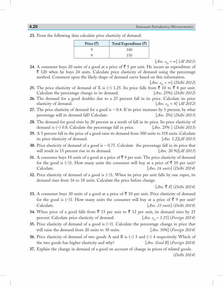
Saraswati Introductory Microeconomics4.20
23. From the following data calculate price elasticity of demand:
Price (`) Total Expenditure (`)
99
100150
[Ans. eD = ∞] (AI 2011) 24. A consumer buys 20 units of a good at a price of ` 5 per unit. He incurs an expenditure of
` 120 when he buys 24 units. Calculate price elasticity of demand using the percentage method. Comment upon the likely shape of demand curve based on this information.
[Ans. eD = ∞] (Delhi 2012) 25. The price elasticity of demand of X is (–) 1.25. Its price falls from ` 10 to ` 8 per unit.
Calculate the percentage change in its demand. [Ans. 25%] (Delhi 2012) 26. The demand for a good doubles due to a 25 percent fall in its price. Calculate its price
elasticity of demand. [Ans. eD = 4] (AI 2012) 27. The price elasticity of demand for a good is – 0.4. If its price increases by 5 percent, by what
percentage will its demand fall? Calculate. [Ans. 2%] (Delhi 2013)
28. The demand for good rises by 20 percent as a result of fall in its price. Its price elasticity of demand is (–) 0.8. Calculate the percentage fall in price. [Ans. 25% ] (Delhi 2013)
29. A 5 percent fall in the price of a good raise its demand from 300 units to 318 units. Calculate its price elasticity of demand. [Ans. 1.2](AI 2013)
30. Price elasticity of demand of a good is – 0.75. Calculate the percentage fall in its price that will result in 15 percent rise in its demand. [Ans. 20 %](AI 2013)
31. A consumer buys 18 units of a good at a price of ` 9 per unit. The price elasticity of demand for the good is (–)1. How many units the consumer will buy at a price of ` 10 per unit? Calculate. [Ans. 16 units] (Delhi 2014)
32. Price elasticity of demand of a good is (–)1. When its price per unit falls by one rupee, its demand rises from 16 to 18 units. Calculate the price before change.
[Ans. ` 8] (Delhi 2014)
33. A consumer buys 30 units of a good at a price of ` 10 per unit. Price elasticity of demand for the good is (–)1. How many units the consumer will buy at a price of ` 9 per unit? Calculate. [Ans. 33 units] (Delhi 2014)
34. When price of a good falls from ` 15 per unit to ` 12 per unit, its demand rises by 25 percent. Calculate price elasticity of demand. [Ans. eD = 1.25] (Foreign 2014)
35. Price elasticity of demand of a good is (–)1. Calculate the percentage change in price that will raise the demand from 20 units to 30 units. [Ans. 50%] (Foreign 2014)
36. Price elasticity of demand of two goods A and B is (–) 3 and (–) 4 respectively. Which of the two goods has higher elasticity and why? [Ans. Good B] (Foreign 2014)
37. Explain the change in demand of a good on account of change in prices of related goods. (Delhi 2014)
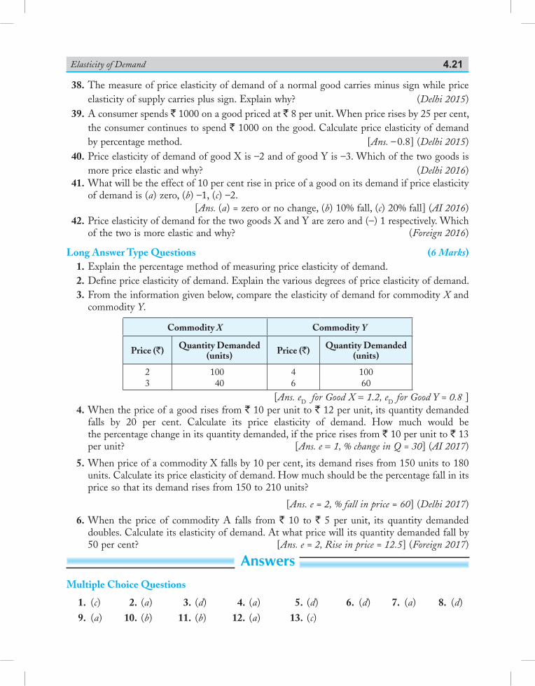
Elasticity of Demand 4.21
38. The measure of price elasticity of demand of a normal good carries minus sign while price elasticity of supply carries plus sign. Explain why? (Delhi 2015)
39. A consumer spends ` 1000 on a good priced at ` 8 per unit. When price rises by 25 per cent, the consumer continues to spend ` 1000 on the good. Calculate price elasticity of demand by percentage method. [Ans. – 0.8] (Delhi 2015)
40. Price elasticity of demand of good X is –2 and of good Y is –3. Which of the two goods is more price elastic and why? (Delhi 2016)
41. What will be the effect of 10 per cent rise in price of a good on its demand if price elasticity of demand is (a) zero, (b) –1, (c) –2.
[Ans. (a) = zero or no change, (b) 10% fall, (c) 20% fall] (AI 2016) 42. Price elasticity of demand for the two goods X and Y are zero and (–) 1 respectively. Which
of the two is more elastic and why? (Foreign 2016)
Long Answer Type Questions (6 Marks) 1. Explain the percentage method of measuring price elasticity of demand. 2. Define price elasticity of demand. Explain the various degrees of price elasticity of demand. 3. From the information given below, compare the elasticity of demand for commodity X and
commodity Y.
Commodity X Commodity Y
Price (`) Quantity Demanded (units) Price (`) Quantity Demanded
(units)
23
100 40
46
10060
[Ans. eD for Good X = 1.2, eD for Good Y = 0.8 ] 4. When the price of a good rises from ` 10 per unit to ` 12 per unit, its quantity demanded
falls by 20 per cent. Calculate its price elasticity of demand. How much would be the percentage change in its quantity demanded, if the price rises from ` 10 per unit to ` 13 per unit? [Ans. e = 1, % change in Q = 30] (AI 2017)
5. When price of a commodity X falls by 10 per cent, its demand rises from 150 units to 180 units. Calculate its price elasticity of demand. How much should be the percentage fall in its price so that its demand rises from 150 to 210 units?
[Ans. e = 2, % fall in price = 60] (Delhi 2017)
6. When the price of commodity A falls from ` 10 to ` 5 per unit, its quantity demanded doubles. Calculate its elasticity of demand. At what price will its quantity demanded fall by 50 per cent? [Ans. e = 2, Rise in price = 12.5] (Foreign 2017)
answersMultiple Choice Questions
1. (c) 2. (a) 3. (d) 4. (a) 5. (d) 6. (d) 7. (a) 8. (d) 9. (a) 10. (b) 11. (b) 12. (a) 13. (c)
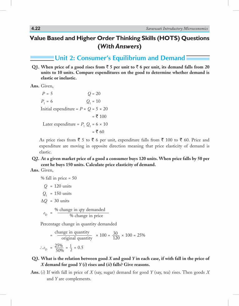
Saraswati Introductory Microeconomics4.22
Value Based and Higher Order Thinking Skills (HOTS) Questions(With Answers)
Unit 2: Consumer’s Equilibrium and Demand Q1. When price of a good rises from ` 5 per unit to ` 6 per unit, its demand falls from 20
units to 10 units. Compare expenditures on the good to determine whether demand is elastic or inelastic.
Ans. Given,
P = 5 Q = 20
P1 = 6 Q1 = 10
Initial expenditure = P × Q = 5 × 20
= ` 100
Later expenditure = P1 Q1 = 6 × 10
= ` 60
As price rises from ` 5 to ` 6 per unit, expenditure falls from ` 100 to ` 60. Price and expenditure are moving in opposite direction meaning that price elasticity of demand is elastic.
Q2. At a given market price of a good a consumer buys 120 units. When price falls by 50 per cent he buys 150 units. Calculate price elasticity of demand.
Ans. Given,
% fall in price = 50
Q = 120 units
Q1 = 150 units
DQ = 30 units
eD = % change in qty demanded
_______________________ % change in price
Percentage change in quantity demanded
= change in quantity
________________ original quantity
× 100 = 30 ____ 120 × 100 = 25%
\ eD = 25% ____ 50%
= 1 __ 2 = 0.5
Q3. What is the relation between good X and good Y in each case, if with fall in the price of X demand for good Y (i) rises and (ii) falls? Give reasons.
Ans. (i) If with fall in price of X (say, sugar) demand for good Y (say, tea) rises. Then goods X and Y are complements.
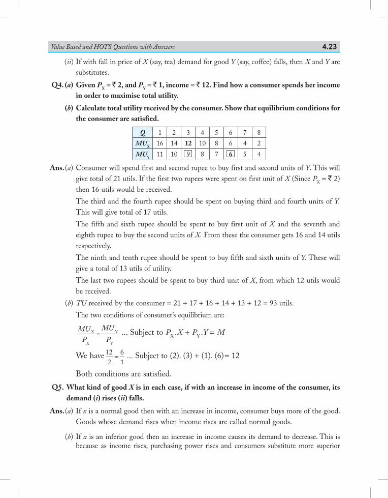
Value Based and HOTS Questions with Answers 4.23
(ii) If with fall in price of X (say, tea) demand for good Y (say, coffee) falls, then X and Y are substitutes.
Q4. (a) Given PX = ` 2, and PY = ` 1, income = ` 12. Find how a consumer spends her income in order to maximise total utility.
(b) Calculate total utility received by the consumer. Show that equilibrium conditions for the consumer are satisfied.
Q 1 2 3 4 5 6 7 8
MUX 16 14 12 10 8 6 4 2
MUY 11 10 9 8 7 6 5 4
Ans. (a) Consumer will spend first and second rupee to buy first and second units of Y. This will give total of 21 utils. If the first two rupees were spent on first unit of X (Since PX = ` 2) then 16 utils would be received.
The third and the fourth rupee should be spent on buying third and fourth units of Y. This will give total of 17 utils.
The fifth and sixth rupee should be spent to buy first unit of X and the seventh and eighth rupee to buy the second units of X. From these the consumer gets 16 and 14 utils respectively.
The ninth and tenth rupee should be spent to buy fifth and sixth units of Y. These will give a total of 13 utils of utility.
The last two rupees should be spent to buy third unit of X, from which 12 utils would be received.
(b) TU received by the consumer = 21 + 17 + 16 + 14 + 13 + 12 = 93 utils.
The two conditions of consumer’s equilibrium are:
MUP
MU
PX
X
Y
Y
= ... Subject to PX .X + PY .Y = M
We have122
= 61 ... Subject to (2). (3) + (1). (6) = 12
Both conditions are satisfied.
Q5. What kind of good X is in each case, if with an increase in income of the consumer, its demand (i) rises (ii) falls.
Ans. (a) If x is a normal good then with an increase in income, consumer buys more of the good. Goods whose demand rises when income rises are called normal goods.
(b) If x is an inferior good then an increase in income causes its demand to decrease. This is because as income rises, purchasing power rises and consumers substitute more superior
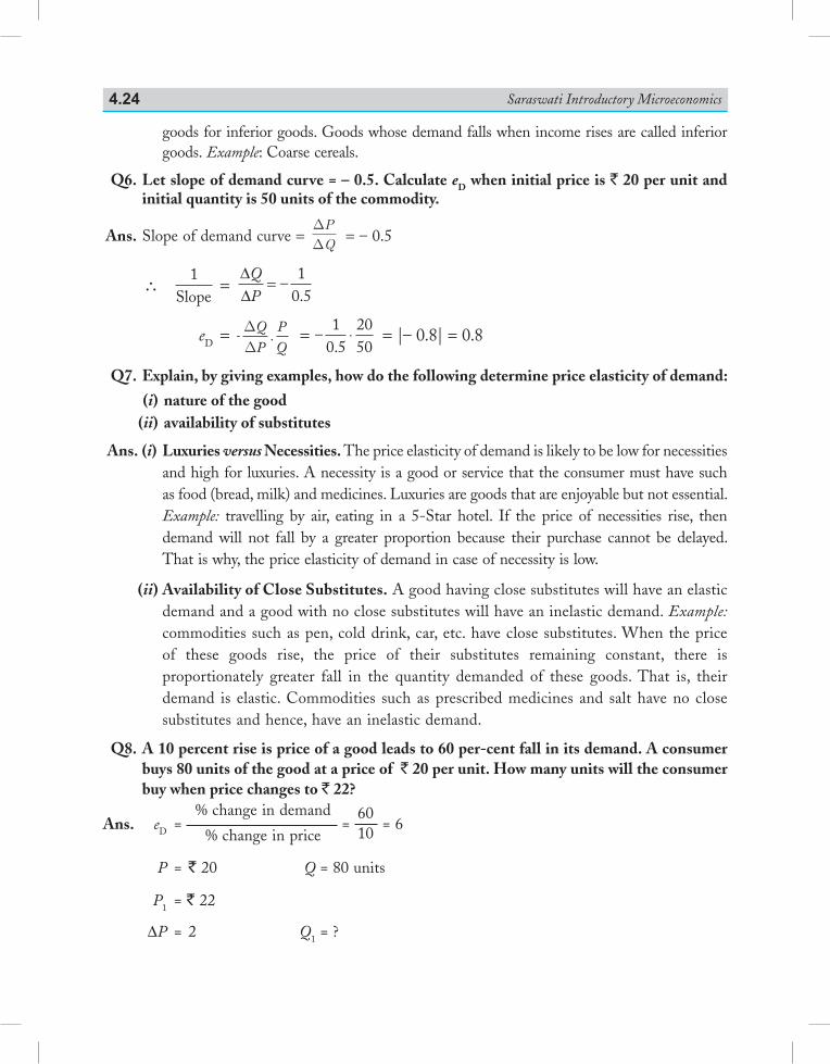
Saraswati Introductory Microeconomics4.24
goods for inferior goods. Goods whose demand falls when income rises are called inferior goods. Example: Coarse cereals.
Q6. Let slope of demand curve = – 0.5. Calculate eD when initial price is ` 20 per unit and initial quantity is 50 units of the commodity.
Ans. Slope of demand curve = DDPQ
= – 0.5
\ 1
Slope= ∆
∆=Q
P–
.1
0 5 =
1Slope
= ∆∆
=QP
–.1
0 5
eD = – QP
.PQ
DD
= –.1
0 52050
⋅ = |– 0.8| = 0.8
Q7. Explain, by giving examples, how do the following determine price elasticity of demand:
(i) nature of the good (ii) availability of substitutes
Ans. (i) Luxuries versus Necessities. The price elasticity of demand is likely to be low for necessities and high for luxuries. A necessity is a good or service that the consumer must have such as food (bread, milk) and medicines. Luxuries are goods that are enjoyable but not essential. Example: travelling by air, eating in a 5-Star hotel. If the price of necessities rise, then demand will not fall by a greater proportion because their purchase cannot be delayed. That is why, the price elasticity of demand in case of necessity is low.
(ii) Availability of Close Substitutes. A good having close substitutes will have an elastic demand and a good with no close substitutes will have an inelastic demand. Example: commodities such as pen, cold drink, car, etc. have close substitutes. When the price of these goods rise, the price of their substitutes remaining constant, there is proportionately greater fall in the quantity demanded of these goods. That is, their demand is elastic. Commodities such as prescribed medicines and salt have no close substitutes and hence, have an inelastic demand.
Q8. A 10 percent rise is price of a good leads to 60 per-cent fall in its demand. A consumer buys 80 units of the good at a price of ` 20 per unit. How many units will the consumer buy when price changes to ` 22?
Ans. eD = % change in demand
% change in price =
6010 = 6
P = ` 20 Q = 80 units
P1 = ` 22
DP = 2 Q1 = ?
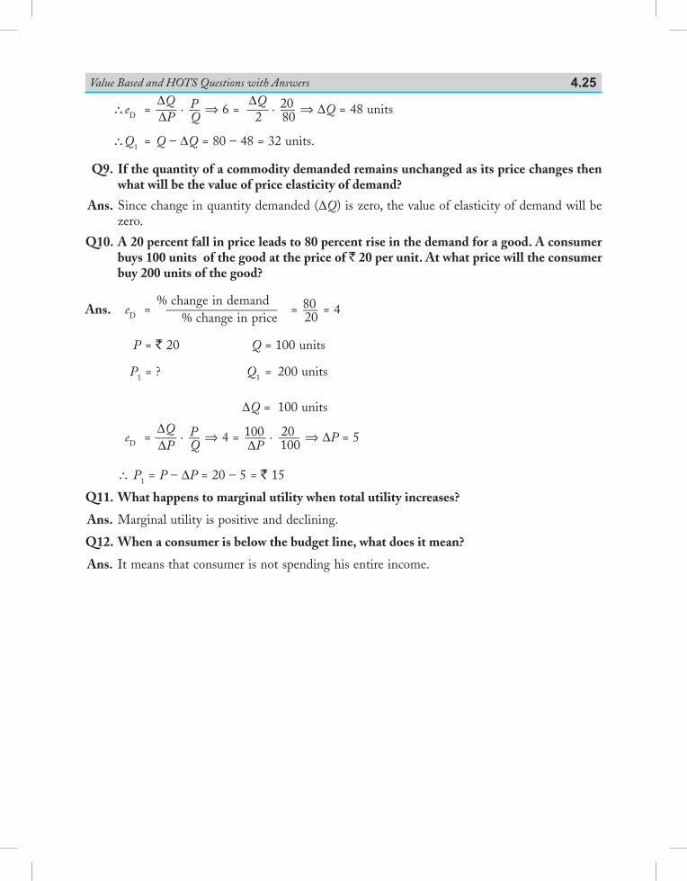
Value Based and HOTS Questions with Answers 4.25
\ eD = DQ
____ DP . P __ Q
⇒ 6 = DQ
____ 2 . 20 ___ 80 ⇒ DQ = 48 units
\ Q1 = Q – DQ = 80 – 48 = 32 units.
Q9. If the quantity of a commodity demanded remains unchanged as its price changes then what will be the value of price elasticity of demand?
Ans. Since change in quantity demanded (DQ) is zero, the value of elasticity of demand will be zero.
Q10. A 20 percent fall in price leads to 80 percent rise in the demand for a good. A consumer buys 100 units of the good at the price of ` 20 per unit. At what price will the consumer buy 200 units of the good?
Ans. eD = % change in demand
_________________ % change in price
= 80 ___ 20 = 4
P = ` 20 Q = 100 units
P1 = ? Q1 = 200 units
DQ = 100 units
eD = DQ
____ DP . P __
Q ⇒ 4 = 100 ____ DP
. 20 ____ 100 ⇒ DP = 5
\ P1 = P – DP = 20 – 5 = ` 15
Q11. What happens to marginal utility when total utility increases?
Ans. Marginal utility is positive and declining.
Q12. When a consumer is below the budget line, what does it mean?
Ans. It means that consumer is not spending his entire income.
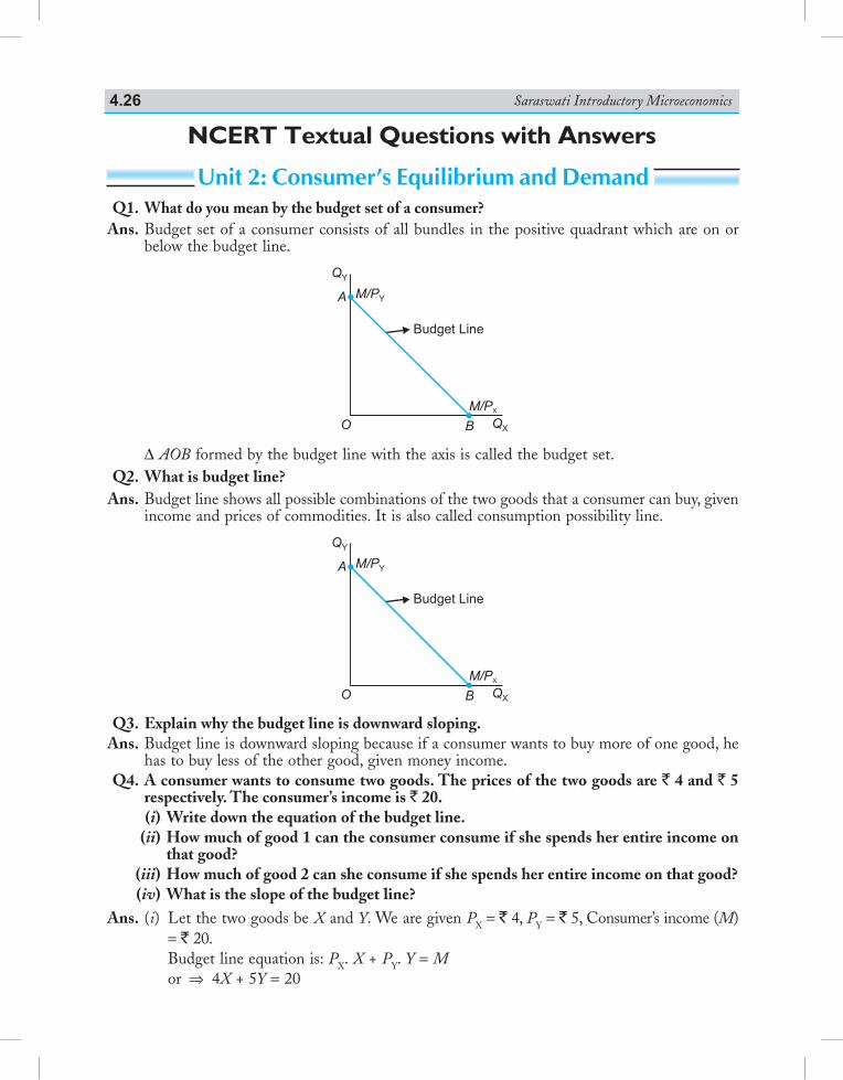
Saraswati Introductory Microeconomics4.26
Q1. What do you mean by the budget set of a consumer? Ans. Budget set of a consumer consists of all bundles in the positive quadrant which are on or
below the budget line.
QY
A M/PY
Budget Line
M/PX
O B QX
D AOB formed by the budget line with the axis is called the budget set. Q2. What is budget line? Ans. Budget line shows all possible combinations of the two goods that a consumer can buy, given
income and prices of commodities. It is also called consumption possibility line.
QY
A M/PY
Budget Line
M/PX
O B QX
Q3. Explain why the budget line is downward sloping. Ans. Budget line is downward sloping because if a consumer wants to buy more of one good, he
has to buy less of the other good, given money income. Q4. A consumer wants to consume two goods. The prices of the two goods are ` 4 and ` 5
respectively. The consumer’s income is ` 20. (i) Write down the equation of the budget line. (ii) How much of good 1 can the consumer consume if she spends her entire income on
that good? (iii) How much of good 2 can she consume if she spends her entire income on that good? (iv) What is the slope of the budget line? Ans. (i) Let the two goods be X and Y. We are given PX = ` 4, PY = ` 5, Consumer’s income (M)
= ` 20. Budget line equation is: PX. X + PY. Y = M or ⇒ 4X + 5Y = 20
NCERT Textual Questions with Answers
Unit 2: Consumer’s Equilibrium and Demand
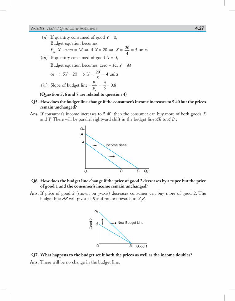
NCERT Textual Questions with Answers 4.27
(ii) If quantity consumed of good Y = 0, Budget equation becomes: PX. X + zero = M ⇒ 4.X = 20 ⇒ X = 20
4 = 5 units
(iii) If quantity consumed of good X = 0,
Budget equation becomes: zero + PY. Y = M
or ⇒ 5Y = 20 ⇒ Y = 205
= 4 units
(iv) Slope of budget line = PP
X
Y
= 45
= 0.8
(Question 5, 6 and 7 are related to question 4)
Q5. How does the budget line change if the consumer’s income increases to ` 40 but the prices remain unchanged?
Ans. If consumer’s income increases to ` 40, then the consumer can buy more of both goods X and Y. There will be parallel rightward shift in the budget line AB to A1B1.
A
A1
BO B1
Income rises
QX
QY
Q6. How does the budget line change if the price of good 2 decreases by a rupee but the price of good 1 and the consumer’s income remain unchanged?
Ans. If price of good 2 (shown on y-axis) decreases consumer can buy more of good 2. The budget line AB will pivot at B and rotate upwards to A1B.
Good
2
A1
O
A
B Good 1
New Budget Line
Q7. What happens to the budget set if both the prices as well as the income doubles?
Ans. There will be no change in the budget line.
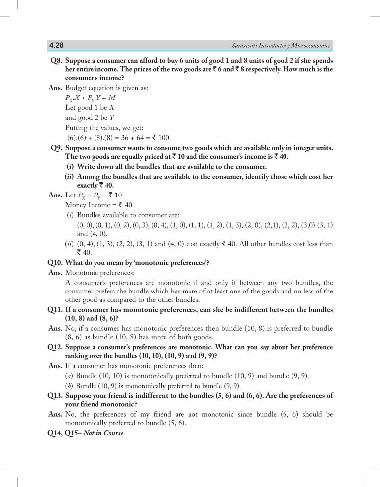
Saraswati Introductory Microeconomics4.28
Q8. Suppose a consumer can afford to buy 6 units of good 1 and 8 units of good 2 if she spends her entire income. The prices of the two goods are ` 6 and ` 8 respectively. How much is the consumer’s income?
Ans. Budget equation is given as: PX.X + PY.Y = M Let good 1 be X and good 2 be Y Putting the values, we get: (6).(6) + (8).(8) = 36 + 64 = ` 100 Q9. Suppose a consumer wants to consume two goods which are available only in integer units.
The two goods are equally priced at ` 10 and the consumer’s income is ` 40. (i) Write down all the bundles that are available to the consumer. (ii) Among the bundles that are available to the consumer, identify those which cost her
exactly ` 40. Ans. Let PX = PY = ` 10 Money Income = ` 40 (i) Bundles available to consumer are: (0, 0), (0, 1), (0, 2), (0, 3), (0, 4), (1, 0), (1, 1), (1, 2), (1, 3), (2, 0), (2,1), (2, 2), (3,0) (3, 1)
and (4, 0). (ii) (0, 4), (1, 3), (2, 2), (3, 1) and (4, 0) cost exactly ` 40. All other bundles cost less than
` 40. Q10. What do you mean by ‘monotonic preferences’? Ans. Monotonic preferences: A consumer’s preferences are monotonic if and only if between any two bundles, the
consumer prefers the bundle which has more of at least one of the goods and no less of the other good as compared to the other bundles.
Q11. If a consumer has monotonic preferences, can she be indifferent between the bundles (10, 8) and (8, 6)?
Ans. No, if a consumer has monotonic preferences then bundle (10, 8) is preferred to bundle (8, 6) as bundle (10, 8) has more of both goods.
Q12. Suppose a consumer’s preferences are monotonic. What can you say about her preference ranking over the bundles (10, 10), (10, 9) and (9, 9)?
Ans. If a consumer has monotonic preferences then: (a) Bundle (10, 10) is monotonically preferred to bundle (10, 9) and bundle (9, 9). (b) Bundle (10, 9) is monotonically preferred to bundle (9, 9). Q13. Suppose your friend is indifferent to the bundles (5, 6) and (6, 6). Are the preferences of
your friend monotonic? Ans. No, the preferences of my friend are not monotonic since bundle (6, 6) should be
monotonically preferred to bundle (5, 6). Q14, Q15– Not in Course
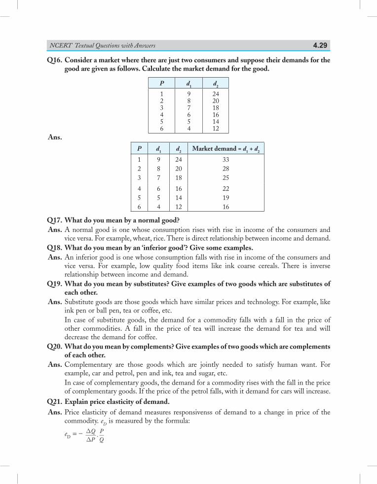
NCERT Textual Questions with Answers 4.29
Q16. Consider a market where there are just two consumers and suppose their demands for the good are given as follows. Calculate the market demand for the good.
P d1 d2
123456
987654
242018161412
Ans.
P d1 d2 Market demand = d1 + d2
123
987
242018
332825
456
654
161412
221916
Q17. What do you mean by a normal good? Ans. A normal good is one whose consumption rises with rise in income of the consumers and
vice versa. For example, wheat, rice. There is direct relationship between income and demand. Q18. What do you mean by an ‘inferior good’? Give some examples. Ans. An inferior good is one whose consumption falls with rise in income of the consumers and
vice versa. For example, low quality food items like ink coarse cereals. There is inverse relationship between income and demand.
Q19. What do you mean by substitutes? Give examples of two goods which are substitutes of each other.
Ans. Substitute goods are those goods which have similar prices and technology. For example, like ink pen or ball pen, tea or coffee, etc.
In case of substitute goods, the demand for a commodity falls with a fall in the price of other commodities. A fall in the price of tea will increase the demand for tea and will decrease the demand for coffee.
Q20. What do you mean by complements? Give examples of two goods which are complements of each other.
Ans. Complementary are those goods which are jointly needed to satisfy human want. For example, car and petrol, pen and ink, tea and sugar, etc.
In case of complementary goods, the demand for a commodity rises with the fall in the price of complementary goods. If the price of the petrol falls, with it demand for cars will increase.
Q21. Explain price elasticity of demand. Ans. Price elasticity of demand measures responsivenss of demand to a change in price of the
commodity. eD is measured by the formula:
eD = – DD
QP
PQ
.
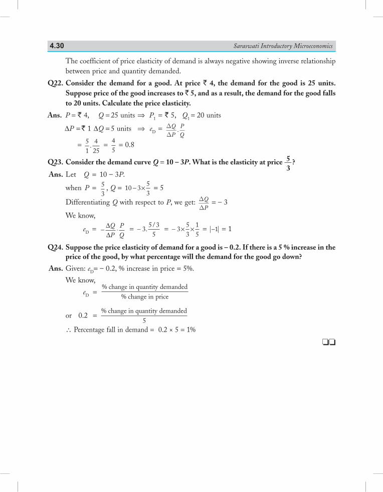
Saraswati Introductory Microeconomics4.30
The coefficient of price elasticity of demand is always negative showing inverse relationship between price and quantity demanded.
Q22. Consider the demand for a good. At price ` 4, the demand for the good is 25 units. Suppose price of the good increases to ` 5, and as a result, the demand for the good falls to 20 units. Calculate the price elasticity.
Ans. P = ` 4, Q = 25 units ⇒ P1 = ` 5, Q1 = 20 units
DP = ̀ 1 DQ = 5 units ⇒ eD = DD
QP
PQ
.
= 51
425
. = 45
= 0.8
Q23. Consider the demand curve Q = 10 – 3P. What is the elasticity at price 53
?
Ans. Let Q = 10 – 3P.
when P = 53
, Q = 10 353
− × = 5
Differentiating Q with respect to P, we get: DD
QP
= – 3
We know,
eD = − ⋅∆∆
QP
PQ
= − 35 3
5.
/ = − × ×353
15
= −1 = 1
Q24. Suppose the price elasticity of demand for a good is – 0.2. If there is a 5 % increase in the price of the good, by what percentage will the demand for the good go down?
Ans. Given: eD= – 0.2, % increase in price = 5%.
We know,
eD = % change in quantity demanded
% change in price
or 0.2 = % change in quantity demanded
5
\ Percentage fall in demand = 0.2 × 5 = 1%
oo

Producer Behaviourand
Supply
UNIT–3
This Unit Contains5. Production Function6. Cost7. Revenue8. Producer’s Equilibrium9. Supply and Elasticity of Supply
5.1 Meaning of Production
Production is defined as the transformation of inputs into output. For example, inputs of sugar cane, capital and labour are used to produce sugar. Production includes not only production of physical goods like cloth, rice, etc., but also production of services like those of a doctor, teacher, lawyer, etc.
5.2 Production function5.2.1 Definition of Production FunctionThe term production function means physical relationship between inputs used and the resulting output. Production function is a purely technical relation which connects the quantity of inputs required to produce a good and the quantity of output produced. Production function is the process of getting the maximum output from a given quantity of inputs in a particular time period. It includes only technically efficient combinations of inputs (i.e., those which minimise the cost of production).A production function is an expression of quantitative relation between change in inputs and the resulting change in output. It is expressed as:
Q = f (i1, i2 ..... in)
Production Function
Chapter Scheme
5
5.1 Meaning of Production5.2 Production Function 5.2.1DefinitionofProductionFunction 5.2.2 Short–runandLong–run
ProductionFunction5.3 Concepts of Product 5.3.1TotalPhysicalProduct(TPP)orTotal
Product(TP) 5.3.2AverageProduct(AP)orAverage
PhysicalProduct(APP) 5.3.3MarginalProduct(MP)orMarginal
PhysicalProduct(MPP) 5.3.4RelationshipbetweenTP, APandMP 5.3.5RelationshipbetweenTPandMP 5.3.6RelationshipbetweenAPand MP
(General)5.4 Returns to a Factor 5.4.1LawofVariableProportion 5.4.2AssumptionsoftheLaw 5.4.3ThreePhasesofProduction 5.4.4ReasonsBehindIncreasingand
DiminishingReturnstoaFactor 5.4.5PostponementoftheLaw Solved Numerical Problems Points to Remember Test Your Knowledge Answers to MCQs
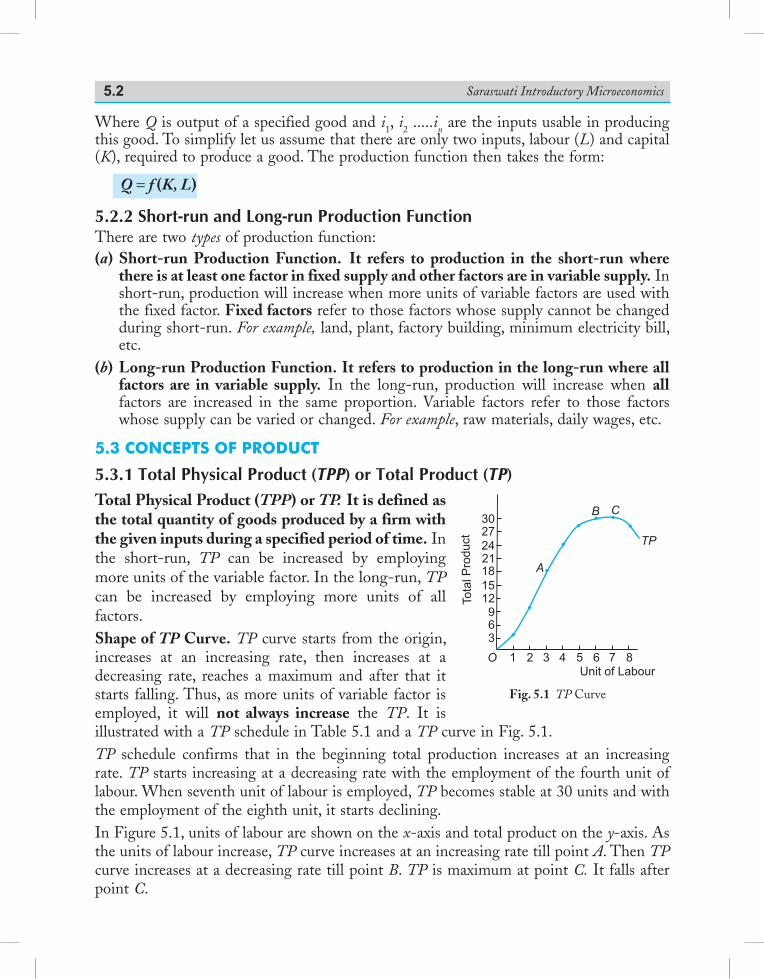
Saraswati Introductory Microeconomics5.2
Where Q is output of a specified good and i1, i2 .....in are the inputs usable in producing this good. To simplify let us assume that there are only two inputs, labour (L) and capital (K), required to produce a good. The production function then takes the form:
Q = f (K, L)
5.2.2 Short-run and Long-run Production FunctionThere are two types of production function:(a) Short-run Production Function. It refers to production in the short-run where
there is at least one factor in fixed supply and other factors are in variable supply. In short-run, production will increase when more units of variable factors are used with the fixed factor. Fixed factors refer to those factors whose supply cannot be changed during short-run. For example, land, plant, factory building, minimum electricity bill, etc.
(b) Long-run Production Function. It refers to production in the long-run where all factors are in variable supply. In the long-run, production will increase when all factors are increased in the same proportion. Variable factors refer to those factors whose supply can be varied or changed. For example, raw materials, daily wages, etc.
5.3 concePts of Product
5.3.1 Total Physical Product (TPP) or Total Product (TP)Total Physical Product (TPP) or TP. It is defined as the total quantity of goods produced by a firm with the given inputs during a specified period of time. In the short-run, TP can be increased by employing more units of the variable factor. In the long-run, TP can be increased by employing more units of all factors.Shape of TP Curve. TP curve starts from the origin, increases at an increasing rate, then increases at a decreasing rate, reaches a maximum and after that it starts falling. Thus, as more units of variable factor is employed, it will not always increase the TP. It is illustrated with a TP schedule in Table 5.1 and a TP curve in Fig. 5.1.TP schedule confirms that in the beginning total production increases at an increasing rate. TP starts increasing at a decreasing rate with the employment of the fourth unit of labour. When seventh unit of labour is employed, TP becomes stable at 30 units and with the employment of the eighth unit, it starts declining.In Figure 5.1, units of labour are shown on the x-axis and total product on the y-axis. As the units of labour increase, TP curve increases at an increasing rate till point A. Then TP curve increases at a decreasing rate till point B. TP is maximum at point C. It falls after point C.
30
27
24
21
18
15
12
9
6
3
O 1 2 3 4 5 6 7 8
A
B C
TP
Tota
lP
roduct
Unit of Labour
Fig. 5.1 TP Curve
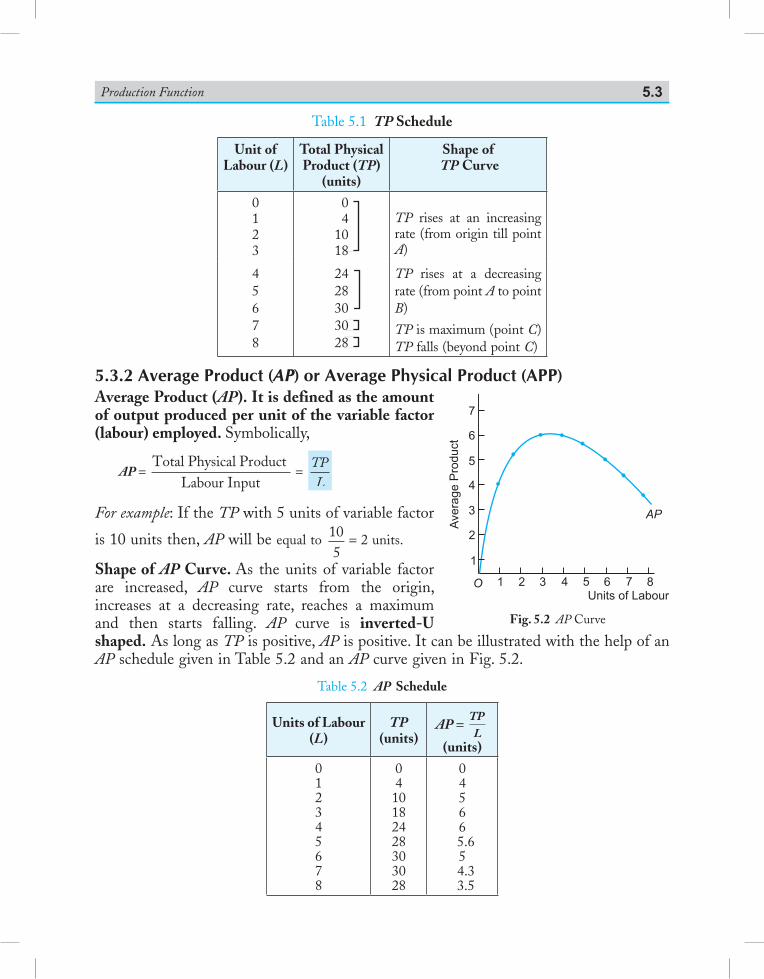
Production Function 5.3
Table 5.1 TP Schedule
Unit ofLabour (L)
Total PhysicalProduct (TP)
(units)
Shape of TP Curve
0123
04
1018
TP rises at an increasing rate (from origin till point A)
45678
2428303028
TP rises at a decreasing rate (from point A to point B)
TP is maximum (point C)TP falls (beyond point C)
5.3.2 Average Product (AP) or Average Physical Product (APP)Average Product (AP). It is defined as the amount of output produced per unit of the variable factor (labour) employed. Symbolically,
AP = Total Physical Pr oduct
Labour Input=
TPL
For example: If the TP with 5 units of variable factor
is 10 units then, AP will be equal to 105
= 2 units.
Shape of AP Curve. As the units of variable factor are increased, AP curve starts from the origin, increases at a decreasing rate, reaches a maximum and then starts falling. AP curve is inverted-U shaped. As long as TP is positive, AP is positive. It can be illustrated with the help of an AP schedule given in Table 5.2 and an AP curve given in Fig. 5.2.
Table 5.2 AP Schedule
Units of Labour (L)
TP(units)
AP = TPL
(units)
012345678
0410182428303028
04566
5.65
4.3 3.5
7
6
5
4
3
2
1
O 1 2 3 4 5 6 7 8
AP
Units of Labour
Ave
rag
eP
rod
uct
Fig. 5.2 AP Curve
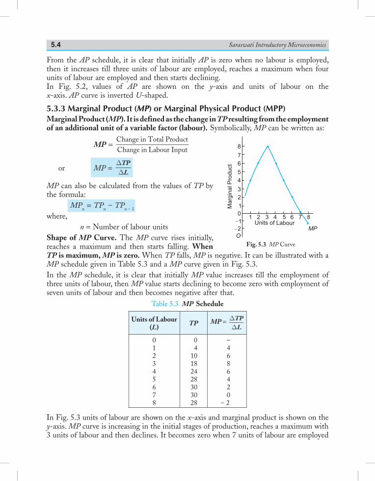
Saraswati Introductory Microeconomics5.4
From the AP schedule, it is clear that initially AP is zero when no labour is employed, then it increases till three units of labour are employed, reaches a maximum when four units of labour are employed and then starts declining.In Fig. 5.2, values of AP are shown on the y-axis and units of labour on the x-axis. AP curve is inverted U-shaped.
5.3.3 Marginal Product (MP) or Marginal Physical Product (MPP)Marginal Product (MP). It is defined as the change in TP resulting from the employment of an additional unit of a variable factor (labour). Symbolically, MP can be written as:
MP = Change in Total ProductChange in Labour Input
or MP = DDTPL
MP can also be calculated from the values of TP by the formula: MPn = TPn – TPn – 1
where, n = Number of labour unitsShape of MP Curve. The MP curve rises initially, reaches a maximum and then starts falling. When TP is maximum, MP is zero. When TP falls, MP is negative. It can be illustrated with a MP schedule given in Table 5.3 and a MP curve given in Fig. 5.3.In the MP schedule, it is clear that initially MP value increases till the employment of three units of labour, then MP value starts declining to become zero with employment of seven units of labour and then becomes negative after that.
Table 5.3 MP Schedule
Units of Labour (L) TP MP = D
DTPL
012345678
04
10182428303028
–468642 0
– 2
In Fig. 5.3 units of labour are shown on the x-axis and marginal product is shown on the y-axis. MP curve is increasing in the initial stages of production, reaches a maximum with 3 units of labour and then declines. It becomes zero when 7 units of labour are employed
Fig. 5.3 MP Curve
Marg
inalP
roduct
Units of Labour
MP
O
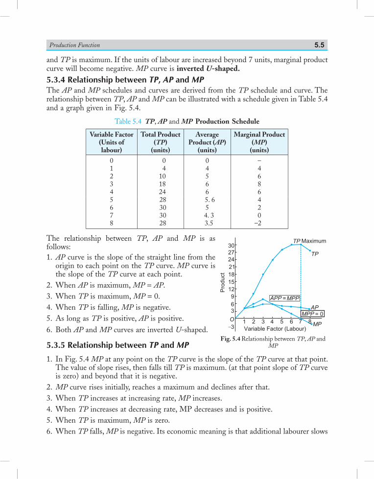
Production Function 5.5
and TP is maximum. If the units of labour are increased beyond 7 units, marginal product curve will become negative. MP curve is inverted U-shaped.5.3.4 Relationship between TP, AP and MPThe AP and MP schedules and curves are derived from the TP schedule and curve. The relationship between TP, AP and MP can be illustrated with a schedule given in Table 5.4 and a graph given in Fig. 5.4.
Table 5.4 TP, AP and MP Production Schedule
Variable Factor (Units of labour)
Total Product (TP)
(units)
Average Product (AP)
(units)
Marginal Product (MP)
(units)
01234
04
101824
04566
–4686
5678
28303028
5. 65
4. 3 3.5
420
–2
The relationship between TP, AP and MP is as follows:1. AP curve is the slope of the straight line from the
origin to each point on the TP curve. MP curve is the slope of the TP curve at each point.
2. When AP is maximum, MP = AP.3. When TP is maximum, MP = 0.4. When TP is falling, MP is negative.5. As long as TP is positive, AP is positive.6. Both AP and MP curves are inverted U-shaped.
5.3.5 Relationship between TP and MP
1. In Fig. 5.4 MP at any point on the TP curve is the slope of the TP curve at that point. The value of slope rises, then falls till TP is maximum. (at that point slope of TP curve is zero) and beyond that it is negative.
2. MP curve rises initially, reaches a maximum and declines after that.3. When TP increases at increasing rate, MP increases.4. When TP increases at decreasing rate, MP decreases and is positive.5. When TP is maximum, MP is zero.6. When TP falls, MP is negative. Its economic meaning is that additional labourer slows
30
27
24
21
18
15
12
9
6
3
O
31 2 3 4 5 6 7
Pro
duct
APP = MPP
TP Maximum
TP
AP
MPP = 0
MPVariable Factor (Labour)
8
Fig. 5.4 Relationship between TP, AP and MP
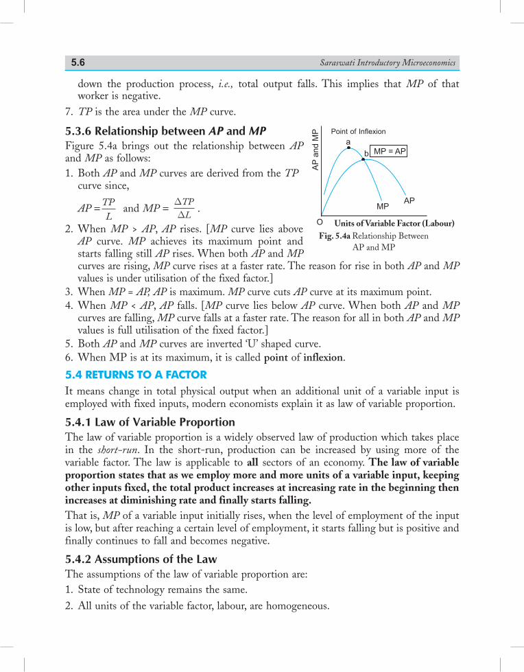
Saraswati Introductory Microeconomics5.6
down the production process, i.e., total output falls. This implies that MP of that worker is negative.
7. TP is the area under the MP curve.
5.3.6 Relationship between AP and MPFigure 5.4a brings out the relationship between AP and MP as follows:1. Both AP and MP curves are derived from the TP
curve since,
AP =TPL
and MP = DD
TPL
.
2. When MP > AP, AP rises. [MP curve lies above AP curve. MP achieves its maximum point and starts falling still AP rises. When both AP and MP curves are rising, MP curve rises at a faster rate. The reason for rise in both AP and MP values is under utilisation of the fixed factor.]
3. When MP = AP, AP is maximum. MP curve cuts AP curve at its maximum point.4. When MP < AP, AP falls. [MP curve lies below AP curve. When both AP and MP
curves are falling, MP curve falls at a faster rate. The reason for all in both AP and MP values is full utilisation of the fixed factor.]
5. Both AP and MP curves are inverted ‘U’ shaped curve.6. When MP is at its maximum, it is called point of inflexion.
5.4 returns to a factorIt means change in total physical output when an additional unit of a variable input is employed with fixed inputs, modern economists explain it as law of variable proportion.
5.4.1 Law of Variable ProportionThe law of variable proportion is a widely observed law of production which takes place in the short-run. In the short-run, production can be increased by using more of the variable factor. The law is applicable to all sectors of an economy. The law of variable proportion states that as we employ more and more units of a variable input, keeping other inputs fixed, the total product increases at increasing rate in the beginning then increases at diminishing rate and finally starts falling.That is, MP of a variable input initially rises, when the level of employment of the input is low, but after reaching a certain level of employment, it starts falling but is positive and finally continues to fall and becomes negative.
5.4.2 Assumptions of the LawThe assumptions of the law of variable proportion are:1. State of technology remains the same.2. All units of the variable factor, labour, are homogeneous.
a
b MP = AP
MPAP
AP
and M
P
O
Fig. 5.4a Relationship Between AP and MP
Units of Variable Factor (Labour)
Point of Inflexion
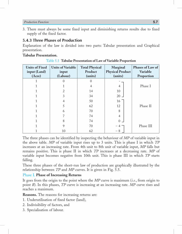
Production Function 5.7
3. There must always be some fixed input and diminishing returns results due to fixed supply of the fixed factor.
5.4.3 Three Phases of ProductionExplanation of the law is divided into two parts: Tabular presentation and Graphical presentation. Tabular Presentation.
Table 5.5 Tabular Presentation of Law of Variable Proportion
Units of Fixed input (Land)
(Acre)
Units of Variable input
(Labour)
Total Physical Product(units)
Marginal Physical Product
(units)
Phases of Law of Variable
Proportion1 0 0 -1 1 4 4 Phase I1 2 14 101 3 34 201 4 50 161 5 62 12 Phase II1 6 70 81 7 74 41 8 74 01 9 70 – 4 Phase III1 10 62 – 8
The three phases can be identified by inspecting the behaviour of MP of variable input in the above table. MP of variable input rises up to 3 units. This is phase I in which TP increases at an increasing rate. From 4th unit to 8th unit of variable input, MP falls but remains positive. This is phase II in which TP increases at a decreasing rate. MP of variable input becomes negative from 10th unit. This is phase III in which TP starts falling.These three phases of the short-run law of production are graphically illustrated by the relationship between TP and MP curves. It is given in Fig. 5.5.Phase I. Phase of Increasing ReturnsIt goes from the origin to the point where the MP curve is maximum (i.e., from origin to point B). In this phases, TP curve is increasing at an increasing rate. MP curve rises and reaches a maximum.Reasons. The reasons for increasing returns are:1. Underutilisation of fixed factor (land),2. Indivisibility of factors, and3. Specialisation of labour.
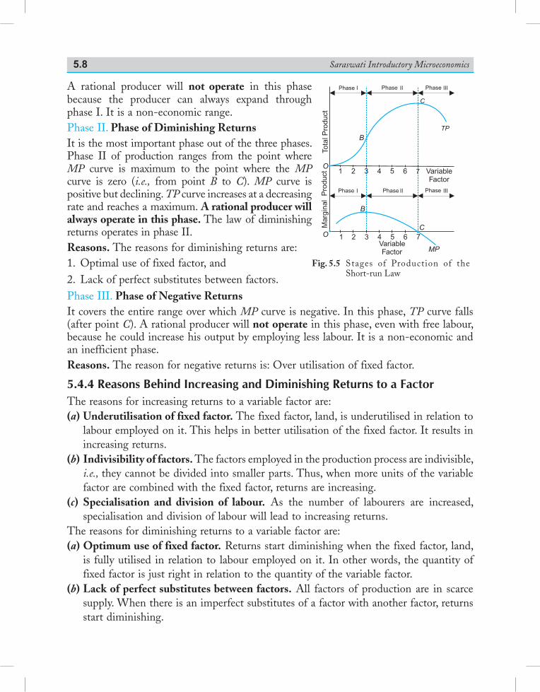
Saraswati Introductory Microeconomics5.8
A rational producer will not operate in this phase because the producer can always expand through phase I. It is a non-economic range.Phase II. Phase of Diminishing ReturnsIt is the most important phase out of the three phases. Phase II of production ranges from the point where MP curve is maximum to the point where the MP curve is zero (i.e., from point B to C). MP curve is positive but declining. TP curve increases at a decreasing rate and reaches a maximum. A rational producer will always operate in this phase. The law of diminishing returns operates in phase II.Reasons. The reasons for diminishing returns are:1. Optimal use of fixed factor, and2. Lack of perfect substitutes between factors.Phase III. Phase of Negative Returns It covers the entire range over which MP curve is negative. In this phase, TP curve falls (after point C). A rational producer will not operate in this phase, even with free labour, because he could increase his output by employing less labour. It is a non-economic and an inefficient phase.Reasons. The reason for negative returns is: Over utilisation of fixed factor.
5.4.4 Reasons Behind Increasing and Diminishing Returns to a FactorThe reasons for increasing returns to a variable factor are:(a) Underutilisation of fixed factor. The fixed factor, land, is underutilised in relation to
labour employed on it. This helps in better utilisation of the fixed factor. It results in increasing returns.
(b) Indivisibility of factors. The factors employed in the production process are indivisible, i.e., they cannot be divided into smaller parts. Thus, when more units of the variable factor are combined with the fixed factor, returns are increasing.
(c) Specialisation and division of labour. As the number of labourers are increased, specialisation and division of labour will lead to increasing returns.
The reasons for diminishing returns to a variable factor are:(a) Optimum use of fixed factor. Returns start diminishing when the fixed factor, land,
is fully utilised in relation to labour employed on it. In other words, the quantity of fixed factor is just right in relation to the quantity of the variable factor.
(b) Lack of perfect substitutes between factors. All factors of production are in scarce supply. When there is an imperfect substitutes of a factor with another factor, returns start diminishing.
Fig. 5.5 Stages of Production of the Short-run Law
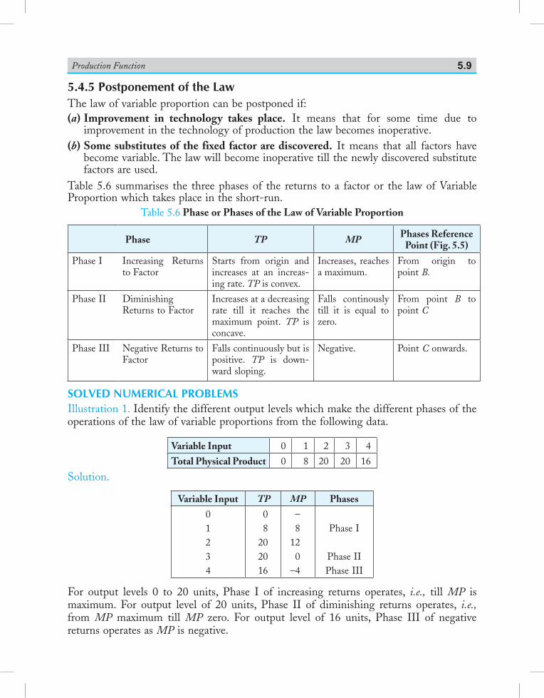
Production Function 5.9
5.4.5 Postponement of the LawThe law of variable proportion can be postponed if:(a) Improvement in technology takes place. It means that for some time due to
improvement in the technology of production the law becomes inoperative.(b) Some substitutes of the fixed factor are discovered. It means that all factors have
become variable. The law will become inoperative till the newly discovered substitute factors are used.
Table 5.6 summarises the three phases of the returns to a factor or the law of Variable Proportion which takes place in the short-run.
Table 5.6 Phase or Phases of the Law of Variable Proportion
Phase TP MP Phases Reference Point (Fig. 5.5)
Phase I Increasing Returns to Factor
Starts from origin and increases at an increas-ing rate. TP is convex.
Increases, reaches a maximum.
From origin to point B.
Phase II Diminishing Returns to Factor
Increases at a decreasing rate till it reaches the maximum point. TP is concave.
Falls continously till it is equal to zero.
From point B to point C
Phase III Negative Returns to Factor
Falls continuously but is positive. TP is down-ward sloping.
Negative. Point C onwards.
SoLVeD NuMeRIcAL PRoBLeMSIllustration 1. Identify the different output levels which make the different phases of the operations of the law of variable proportions from the following data.
Variable Input 0 1 2 3 4
Total Physical Product 0 8 20 20 16
Solution.
Variable Input TP MP Phases
01234
08
202016
–8
120
–4
Phase I
Phase IIPhase III
For output levels 0 to 20 units, Phase I of increasing returns operates, i.e., till MP is maximum. For output level of 20 units, Phase II of diminishing returns operates, i.e., from MP maximum till MP zero. For output level of 16 units, Phase III of negative returns operates as MP is negative.
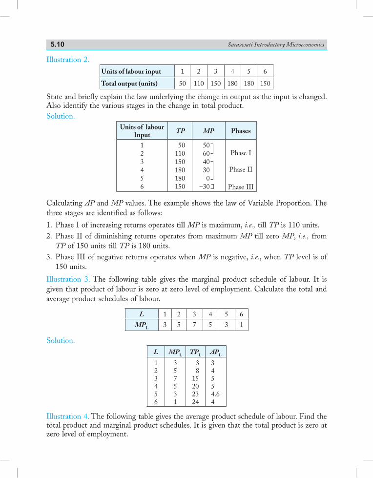
Saraswati Introductory Microeconomics5.10
Illustration 2. Units of labour input 1 2 3 4 5 6
Total output (units) 50 110 150 180 180 150
State and briefly explain the law underlying the change in output as the input is changed. Also identify the various stages in the change in total product.Solution.
Units of labour Input TP MP Phases
123456
50110150180180150
506040300
–30
Phase I
Phase II
Phase III
Calculating AP and MP values. The example shows the law of Variable Proportion. The three stages are identified as follows:
1. Phase I of increasing returns operates till MP is maximum, i.e., till TP is 110 units.2. Phase II of diminishing returns operates from maximum MP till zero MP, i.e., from
TP of 150 units till TP is 180 units.3. Phase III of negative returns operates when MP is negative, i.e., when TP level is of
150 units.
Illustration 3. The following table gives the marginal product schedule of labour. It is given that product of labour is zero at zero level of employment. Calculate the total and average product schedules of labour.
L 1 2 3 4 5 6
MPL 3 5 7 5 3 1
Solution.L MPL TPL APL
123456
357531
3 815202324
34554.64
Illustration 4. The following table gives the average product schedule of labour. Find the total product and marginal product schedules. It is given that the total product is zero at zero level of employment.
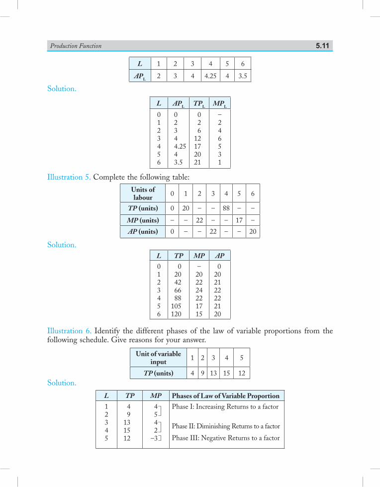
Production Function 5.11
L 1 2 3 4 5 6
APL 2 3 4 4.25 4 3.5
Solution.
L APL TPL MPL
0123456
02344.2543.5
02
612172021
–246531
Illustration 5. Complete the following table:
Units of labour 0 1 2 3 4 5 6
TP (units) 0 20 – – 88 – –
MP (units) – – 22 – – 17 –
AP (units) 0 – – 22 – – 20
Solution.L TP MP AP
0123456
020426688
105120
–202224221715
0202122222120
Illustration 6. Identify the different phases of the law of variable proportions from the following schedule. Give reasons for your answer.
Unit of variable input 1 2 3 4 5
TP (units) 4 9 13 15 12Solution.
L TP MP Phases of Law of Variable Proportion
12345
49
131512
4542
–3
Phase I: Increasing Returns to a factor
Phase II: Diminishing Returns to a factor
Phase III: Negative Returns to a factor
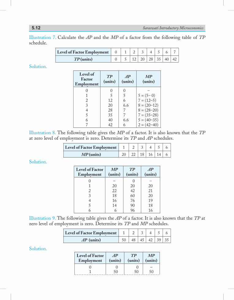
Saraswati Introductory Microeconomics5.12
Illustration 7. Calculate the AP and the MP of a factor from the following table of TP schedule.
Level of Factor Employment 0 1 2 3 4 5 6 7
TP (units) 0 5 12 20 28 35 40 42
Solution.
Level of Factor
Employment
TP (units)
AP(units)
MP(units)
01234567
05
122028354042
0566.6776.66
–5 = (5– 0)7 = (12–5)8 = (20–12)8 = (28–20)7 = (35–28)5 = (40–35)2 = (42–40)
Illustration 8. The following table gives the MP of a factor. It is also known that the TP at zero level of employment is zero. Determine its TP and AP schedules.
Level of Factor Employment 1 2 3 4 5 6
MP (units) 20 22 18 16 14 6
Solution.
Level of Factor Employment
MP (units)
TP(units)
AP(units)
0123456
–20221816146
0204260769096
–202120191816
Illustration 9. The following table gives the AP of a factor. It is also known that the TP at zero level of employment is zero. Determine its TP and MP schedules.
Level of Factor Employment 1 2 3 4 5 6
AP (units) 50 48 45 42 39 35
Solution. Level of Factor
EmploymentAP
(units)TP
(units)MP
(units)
01
050
050
–50
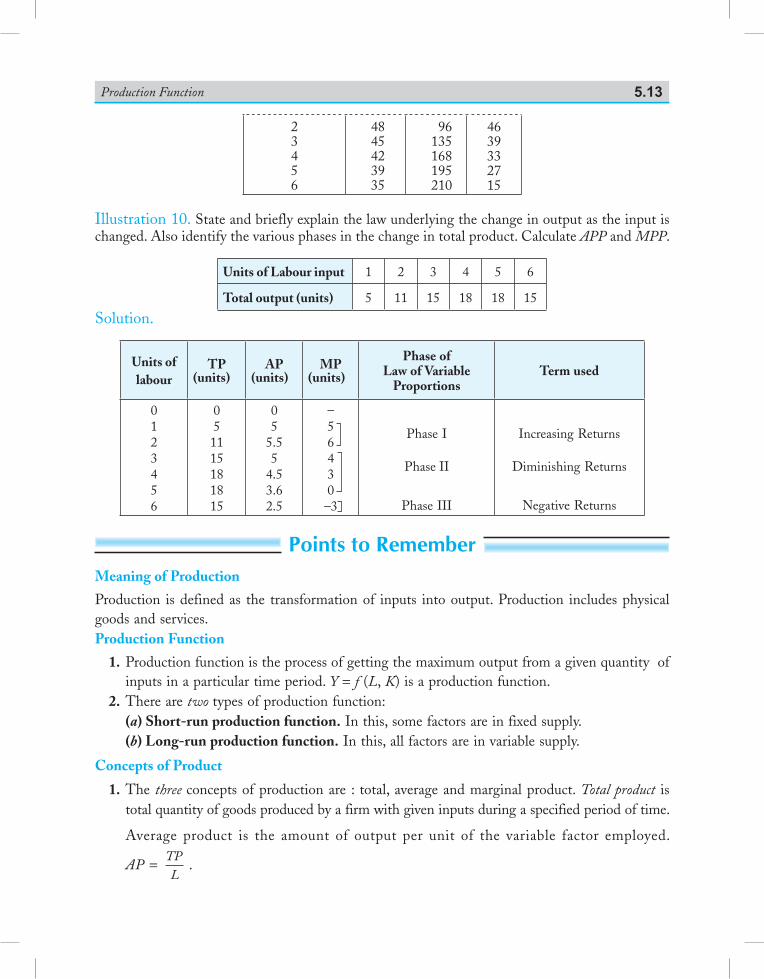
Production Function 5.13
23456
4845423935
96135168195 210
4639332715
Illustration 10. State and briefly explain the law underlying the change in output as the input is changed. Also identify the various phases in the change in total product. Calculate APP and MPP.
Units of Labour input 1 2 3 4 5 6
Total output (units) 5 11 15 18 18 15
Solution.
Units of labour
TP(units)
AP(units)
MP(units)
Phase of Law of Variable
ProportionsTerm used
0123456
051115181815
05
5.55
4.53.62.5
– 56430–3
Phase I
Phase II
Phase III
Increasing Returns
Diminishing Returns
Negative Returns
Points to RememberMeaning of Production
Production is defined as the transformation of inputs into output. Production includes physical goods and services.Production Function
1. Production function is the process of getting the maximum output from a given quantity of inputs in a particular time period. Y = f (L, K) is a production function.
2. There are two types of production function:(a) Short-run production function. In this, some factors are in fixed supply.(b) Long-run production function. In this, all factors are in variable supply.
Concepts of Product
1. The three concepts of production are : total, average and marginal product. Total product is total quantity of goods produced by a firm with given inputs during a specified period of time.
Average product is the amount of output per unit of the variable factor employed.
AP = TPL
.
Saraswati Introductory Microeconomics5.14
Marginal product is the change in total product resulting from the employment of one more
unit of variable factor. MP = DD
TPL
or MPn = TPn – TPn – 1
2. TP curve starts from the origin, rises at an increasing rate, then rises at a decreasing rate, reaches a maximum and then starts falling.
3. Both AP and MP curves are graphically derived from the TP curve. Both AP and MP curves are inverted U-shaped. They have special relationship which is as follows:(a) MP > AP, when AP is rising.(b) MP = AP, when AP is at its maximum.(c) MP < AP, when AP is falling.
The Law of Variable Proportion
1. Law of variable proportion is a widely observed short-run law. 2. The law states that ‘when total output of a commodity is increased by adding units of a variable
factor, while the quantities of other inputs are held constant, the increase in total production, after some point, becomes smaller and smaller’. Initially MP rises and then falls. In law of diminishing MP, MP of variable input falls when one input is combined with fixed input.
3. TP and MP curves are graphically drawn to illustrate the law of Variable Proportions. The three stages or phases are partitioned into increasing, diminishing and negative returns.
4. A rational producer will always operate in Stage II with Diminishing Returns. In this stage MP curve is declining but positive. The reasons for diminishing returns are: (a) Optimal use of fixed factor. (b) Lack of perfect substitutes between factors.
5. Law can be postponed if (a) there is an improvement in technology, (b) new substitutes of fixed factors are discovered.
Test Your KnowledgeVery Short Answer Type Questions (1 Mark) 1. Distinguish between short-run and long-run production function.
2. Define production function. (Foreign 2013,14)
3. Define Law of Variable Proportion.
4. Give meaning of ‘returns to a factor’. (AI 2009, Delhi 2014) 5. How is marginal product calculated? (Foreign 2013) 6. Defi ne marginal product. (AI 2014)
Multiple Choice Questions
1. Production function means:
(a) Physical relationship between inputs used and output
(b) Technical relationship between inputs used and output
(c) Financial relationship between inputs used and output
(d) Both physical and technical relationship between inputs used and output
Production Function 5.15
2. Short-run production function means:
(a) At least one factor is in fixed supply
(b) Two factors are in fixed supply
(c) All factors are in fixed supply
(d) One factor is in variable supply
3. When TP is falling, then MP is:
(a) Falling (b) Negative
(c) Zero (d) Maximum
4. When TP is maximum, MP is:
(a) Falling (b) Negative
(c) Zero (d) Maximum
5. When TP is at its point of inflexion, the MP is:
(a) Falling (b) Negative
(c) Zero (d) Maximum
6. When AP = MP, AP is:
(a) Falling (b) Negative
(c) Zero (d) Maximum
7. Law of Variable Proportions holds when:
(a) State of technology is same
(b) All units of variable factor are homogeneous
(c) There is at least one fixed factor
(d) All of the above
8. Stage II of Law of Variable Proportions is called:
(a) Diminishing returns
(b) Decreasing returns
(c) Falling returns
(d) Negative returns
Short Answer Type Questions (3/4 Marks)
1. Differentiate between fixed factor and variable factor.
2. What is the relationship between AP and MP curves?
3. What are the reasons behind increasing returns to a factor?
4. Explain the relationship between Marginal Physical Product (MP) and Average Physical Product (AP) with the help of a diagram. (Delhi 2012)
Saraswati Introductory Microeconomics5.16
5. What does the Law of Variable Proportions show? State the behaviour of total product according to this law. (Foreign 2009, Delhi 2012)
6. What does the Law of Variable Proportions show? State the behaviour of marginal product according to this law. (AI 2012)
7. Complete the following table: (Delhi 2013)
Units ofLabour
Average Product(Units)
Marginal Product(Units)
1 8 .....2 10 .....3 ..... 104 9 .....5 ..... 46 7 .....
[Ans: AP = 10, 8, MP = 8, 12, 6, 2] 8. Complete the following table : (Delhi 2013)
Units ofLabour
Average Product(Units)
Marginal Product(Units)
1 16 .....
2 20 .....
3 ..... 20
4 18 .....
5 ..... 8
6 14 .....
[Ans: AP = 20, 16, MP = 16, 24, 12, 4]
9. Explain the law of variable proportions. Use diagram. (AI 2014) 10. State the behaviour of marginal product in the law of variable proportions. Explain the
causes of this behaviour. (Delhi 2014) 11. State the different phases of change in total product according to the Law of Variable
Proportions. Use diagram. (Foreign 2014) 12. Define production function. Distinguish between short run and long run production
functions. (Delhi 2016) 13. Define marginal product. State the behaviour of marginal product when only one input is
increased and other inputs are held constant. (AI 2016)
Production Function 5.17
14. State different phases of the law of variable proportions on the basis of total product. Use diagram. (Delhi 2017)
15. Give the meaning and characteristics of production possibility frontier. (AI 2017) 16. Give the behaviour of marginal product and total product as more and more units of only
one input are employed while keeping other inputs as constant. (AI 2017) 17. State the different phases in the behaviour of total product in the law of variable proportions.
Also, show the same in a diagram. (Foreign 2017)
Long Answer Type Questions (6 Marks)
1. What are the three stages of production? Where will a rational producer operate?
2. Calculate APPs and MPPs of a factor. Also identify the various stages of production.
Units of Labour 1 2 3 4 5 6
Total Physical Product (units) 5 11 15 18 18 15
3. What are increasing returns to factor? How do they arise?
4. Identify the different output levels which make the different phases of the operations of the law of variable proportions from the following data. Calculate APP and MPP.
Variable Input 0 1 2 3 4
Total Physical Product (units) 0 8 20 20 16
5. What are the different phases in the behaviour of total product in the law of variable proportions? Use diagram. Also give reasons behind the behaviour in each phase.
(Delhi 2012)
6. Explain the law of variable proportions with the help of total product and marginal product curves. (Delhi 2010, AI 2012, 2013)
7. What type of changes take place in total product and marginal product when there are
(a) increasing returns to a factor?
(b) diminishing returns to a factor?
Why do these changes take place? (Foreign 2010)
8. State the phases of changes in total product in the Law of Variable Proportions. Also explain the reason behind each phase. Use diagram. (Foreign 2011, 12)
9. Giving reasons, state whether the following statements are true or false : (AI 2013)
(i) Average product will increase only when marginal product increases.
(iii) Under diminishing returns to a factor, total product continues to increase till marginal product reaches zero.
Saraswati Introductory Microeconomics5.18
10. Explain the Law of Variable Proportions. Use diagram. (Foreign 2013)
11. State the different phases of changes in Total Product and Marginal Product in the Law of Variable Proportions. Also show the same in a single diagram. (Delhi 2015)
12. What type of production function is this in which only one input is increased and others kept constant? State the behaviour of total product in this production function.
(Foreign 2016)
AnswersMultiple Choice Questions
1. (d) 2. (a) 3. (b) 4. (c) 5. (d) 6. (d) 7. (d) 8. (a)
6.1 Cost and Cost funCtion
Cost is a derived function. It is derived from production function which describes the most efficient method of producing a commodity. Cost of producing a commodity is the payment made to the factors of production which are used in the production of that commodity.Cost FunctionA cost function shows the functional relationship between output and cost of production. It gives the least cost combinations of inputs corresponding to different levels of output.Cost function is given as: C = f (Q), ceteris paribuswhere, C = Cost Q = Output
6.2 types of CostThe time factor is very important in the theory of cost. The time period is classified into two categories: short-run and long-run. Accordingly there are two types of costs:
6.2.1 Short-run CostsThe short-run costs are the costs over a period during which some factors are in fixed supply, like plant, machinery, etc. It is a sum total of fixed cost and variable cost incurred
Cost
Chapter Scheme
6
6.1 Cost and Cost Function6.2 Types of Cost 6.2.1 Short-run Costs 6.2.2 Long-run Costs 6.2.3 Explicit Cost and Implicit Cost 6.3 Total Cost (TC=TFC+TVC) 6.3.1 Total Fixed Cost or Supplementary Cost 6.3.2 Total Variable Cost 6.3.3 Total Cost6.4 Average Cost (AC = AFC + AVC) 6.4.1 Average Fixed Cost
6.4.2 Average Variable Cost 6.4.3 Average Cost (AC) or Average Total
Cost (ATC)6.5 Relationship between AC and AVC Curves6.6 Marginal Cost (MC)6.7 Relationship between TVC and MC Curves6.8 Relationship between AC and MC Curves6.9 Relationship between AVC and MC Curves6.10 Long-run Cost Curves (Only for Reference) Solved Numerical Problems Points to Remember Test Your Knowledge Answers to MCQs
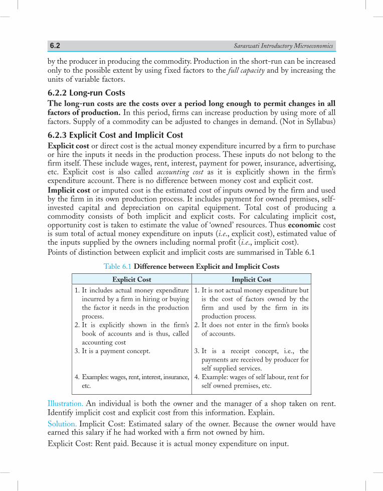
Saraswati Introductory Microeconomics6.2
by the producer in producing the commodity. Production in the short-run can be increased only to the possible extent by using f ixed factors to the full capacity and by increasing the units of variable factors.
6.2.2 Long-run CostsThe long-run costs are the costs over a period long enough to permit changes in all factors of production. In this period, firms can increase production by using more of all factors. Supply of a commodity can be adjusted to changes in demand. (Not in Syllabus)
6.2.3 Explicit Cost and Implicit CostExplicit cost or direct cost is the actual money expenditure incurred by a firm to purchase or hire the inputs it needs in the production process. These inputs do not belong to the firm itself. These include wages, rent, interest, payment for power, insurance, advertising, etc. Explicit cost is also called accounting cost as it is explicitly shown in the firm’s expenditure account. There is no difference between money cost and explicit cost. Implicit cost or imputed cost is the estimated cost of inputs owned by the firm and used by the firm in its own production process. It includes payment for owned premises, self-invested capital and depreciation on capital equipment. Total cost of producing a commodity consists of both implicit and explicit costs. For calculating implicit cost, opportunity cost is taken to estimate the value of ‘owned’ resources. Thus economic cost is sum total of actual money expenditure on inputs (i.e., explicit cost), estimated value of the inputs supplied by the owners including normal profit (i.e., implicit cost).Points of distinction between explicit and implicit costs are summarised in Table 6.1
Table 6.1 Difference between Explicit and Implicit Costs
Explicit Cost Implicit Cost
1. It includes actual money expenditure incurred by a firm in hiring or buying the factor it needs in the production process.
2. It is explicitly shown in the firm’s book of accounts and is thus, called accounting cost
3. It is a payment concept.
4. Examples: wages, rent, interest, insurance, etc.
1. It is not actual money expenditure but is the cost of factors owned by the firm and used by the firm in its production process.
2. It does not enter in the firm’s books of accounts.
3. It is a receipt concept, i.e., the payments are received by producer for self supplied services.
4. Example: wages of self labour, rent for self owned premises, etc.
Illustration. An individual is both the owner and the manager of a shop taken on rent. Identify implicit cost and explicit cost from this information. Explain.Solution. Implicit Cost: Estimated salary of the owner. Because the owner would have earned this salary if he had worked with a firm not owned by him.Explicit Cost: Rent paid. Because it is actual money expenditure on input.
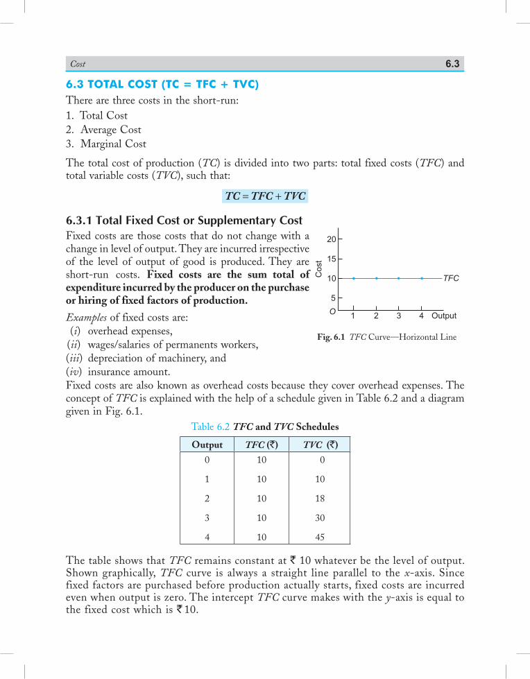
Cost 6.3
Cost
Output
TFC
20
15
10
5
O1 2 3 4
Fig. 6.1 TFC Curve—Horizontal Line
6.3 total Cost (tC = tfC + tVC)There are three costs in the short-run:1. Total Cost 2. Average Cost 3. Marginal Cost
The total cost of production (TC) is divided into two parts: total fixed costs (TFC) and total variable costs (TVC), such that:
TC = TFC + TVC
6.3.1 Total Fixed Cost or Supplementary CostFixed costs are those costs that do not change with a change in level of output. They are incurred irrespective of the level of output of good is produced. They are short-run costs. Fixed costs are the sum total of expenditure incurred by the producer on the purchase or hiring of fixed factors of production.
Examples of fixed costs are: (i) overhead expenses, (ii) wages/salaries of permanents workers, (iii) depreciation of machinery, and (iv) insurance amount.Fixed costs are also known as overhead costs because they cover overhead expenses. The concept of TFC is explained with the help of a schedule given in Table 6.2 and a diagram given in Fig. 6.1.
Table 6.2 TFC and TVC Schedules
Output TFC (`) TVC (`)
0
1
2
3
4
10
10
10
10
10
0
10
18
30
45
The table shows that TFC remains constant at ` 10 whatever be the level of output. Shown graphically, TFC curve is always a straight line parallel to the x-axis. Since fixed factors are purchased before production actually starts, fixed costs are incurred even when output is zero. The intercept TFC curve makes with the y-axis is equal to the fixed cost which is ` 10.
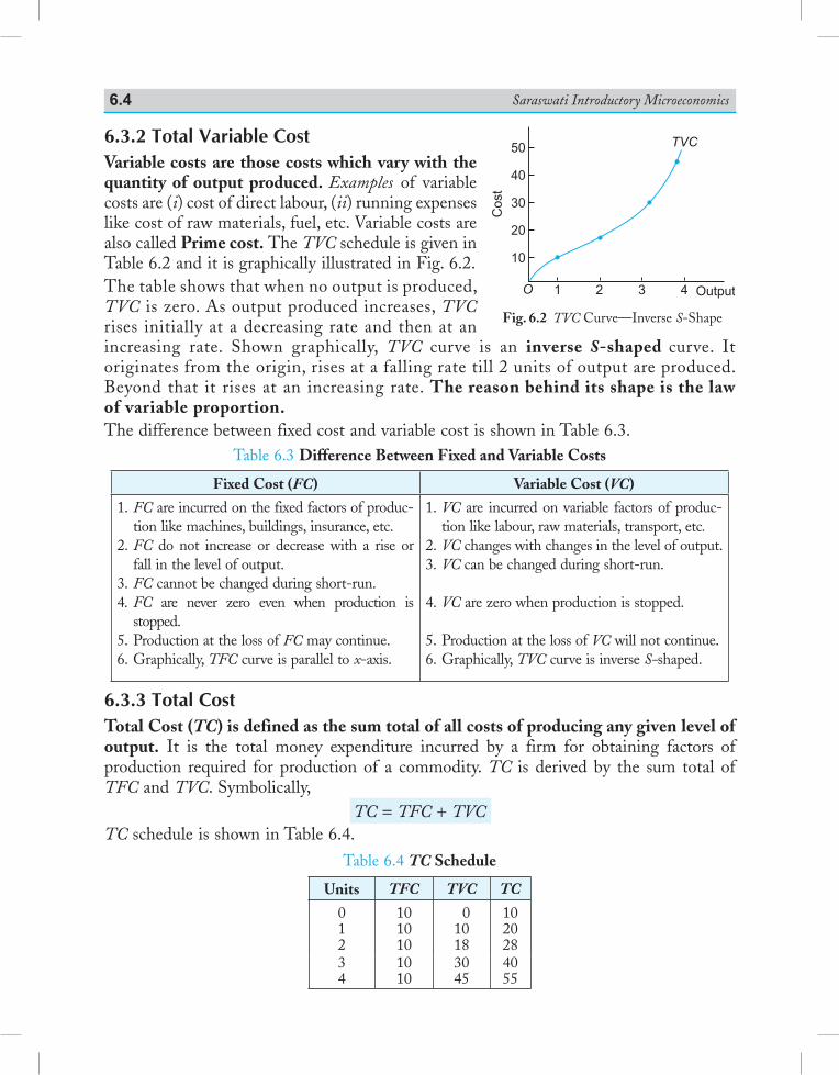
Saraswati Introductory Microeconomics6.4
6.3.2 Total Variable CostVariable costs are those costs which vary with the quantity of output produced. Examples of variable costs are (i) cost of direct labour, (ii) running expenses like cost of raw materials, fuel, etc. Variable costs are also called Prime cost. The TVC schedule is given in Table 6.2 and it is graphically illustrated in Fig. 6.2.The table shows that when no output is produced, TVC is zero. As output produced increases, TVC rises initially at a decreasing rate and then at an increasing rate. Shown graphically, TVC curve is an inverse S-shaped curve. It originates from the origin, rises at a falling rate till 2 units of output are produced. Beyond that it rises at an increasing rate. The reason behind its shape is the law of variable proportion.The difference between fixed cost and variable cost is shown in Table 6.3.
Table 6.3 Difference Between Fixed and Variable Costs
Fixed Cost (FC) Variable Cost (VC)
1. FC are incurred on the fixed factors of produc-tion like machines, buildings, insurance, etc.
2. FC do not increase or decrease with a rise or fall in the level of output.
3. FC cannot be changed during short-run.4. FC are never zero even when production is
stopped.5. Production at the loss of FC may continue.6. Graphically, TFC curve is parallel to x-axis.
1. VC are incurred on variable factors of produc-tion like labour, raw materials, transport, etc.
2. VC changes with changes in the level of output.3. VC can be changed during short-run.
4. VC are zero when production is stopped.
5. Production at the loss of VC will not continue.6. Graphically, TVC curve is inverse S-shaped.
6.3.3 Total CostTotal Cost (TC) is defined as the sum total of all costs of producing any given level of output. It is the total money expenditure incurred by a firm for obtaining factors of production required for production of a commodity. TC is derived by the sum total of TFC and TVC. Symbolically,
TC = TFC + TVCTC schedule is shown in Table 6.4.
Table 6.4 TC Schedule
Units TFC TVC TC
012
101010
01018
102028
34
1010
3045
4055
Fig. 6.2 TVC Curve—Inverse S-Shape
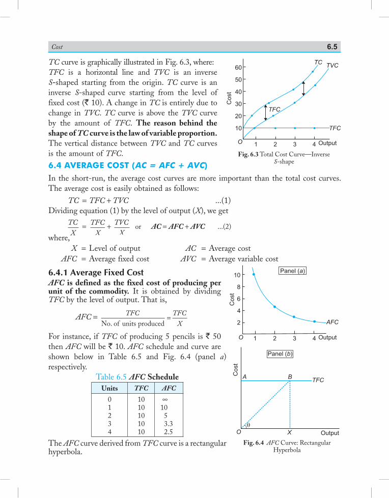
Cost 6.5
TC curve is graphically illustrated in Fig. 6.3, where:TFC is a horizontal line and TVC is an inverse S-shaped starting from the origin. TC curve is an inverse S-shaped curve starting from the level of fixed cost (` 10). A change in TC is entirely due to change in TVC. TC curve is above the TVC curve by the amount of TFC. The reason behind the shape of TC curve is the law of variable proportion. The vertical distance between TVC and TC curves is the amount of TFC.6.4 aVerage Cost (aC = afC + aVC)
In the short-run, the average cost curves are more important than the total cost curves. The average cost is easily obtained as follows: TC = TFC + TVC ...(1) Dividing equation (1) by the level of output (X), we get
TCX
= TFCX
+ TVCX
or AC = AFC + AVC ...(2)
where, X = Level of output AC = Average cost AFC = Average fixed cost AVC = Average variable cost
6.4.1 Average Fixed CostAFC is defined as the fixed cost of producing per unit of the commodity. It is obtained by dividing TFC by the level of output. That is,
AFC = TFC TFC
XNo. of units produced=
For instance, if TFC of producing 5 pencils is ` 50 then AFC will be ` 10. AFC schedule and curve are shown below in Table 6.5 and Fig. 6.4 (panel a) respectively.
Table 6.5 AFC ScheduleUnits TFC AFC
01234
1010101010
∞105
3.32.5
The AFC curve derived from TFC curve is a rectangular hyperbola.
Fig. 6.3 Total Cost Curve—Inverse S-shape
4
Output
Fig. 6.4 AFC Curve: Rectangular Hyperbola
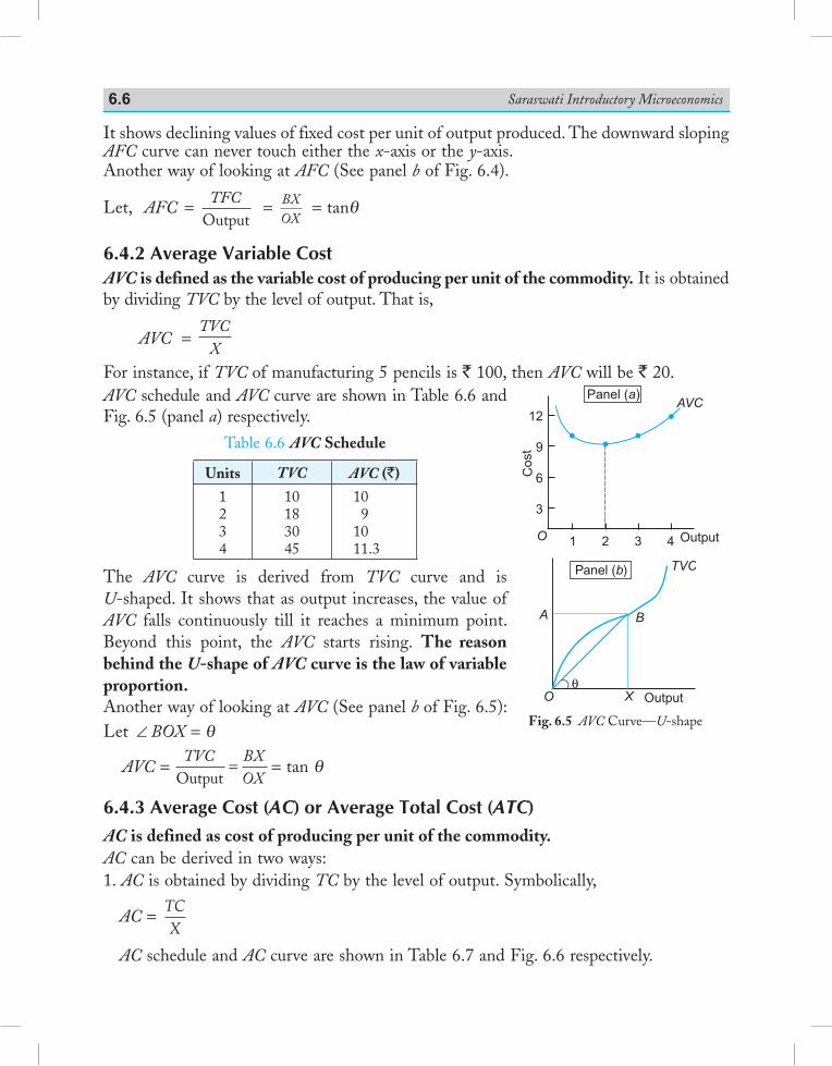
Saraswati Introductory Microeconomics6.6
It shows declining values of fixed cost per unit of output produced. The downward sloping AFC curve can never touch either the x-axis or the y-axis.Another way of looking at AFC (See panel b of Fig. 6.4).
Let, AFC = TFCOutput
= BXOX
= tanθ
6.4.2 Average Variable CostAVC is defined as the variable cost of producing per unit of the commodity. It is obtained by dividing TVC by the level of output. That is,
AVC = TVC
X
For instance, if TVC of manufacturing 5 pencils is ` 100, then AVC will be ` 20. AVC schedule and AVC curve are shown in Table 6.6 and Fig. 6.5 (panel a) respectively.
Table 6.6 AVC Schedule
Units TVC AVC (`)
1234
10183045
10 91011.3
The AVC curve is derived from TVC curve and is U-shaped. It shows that as output increases, the value of AVC falls continuously till it reaches a minimum point. Beyond this point, the AVC starts rising. The reason behind the U-shape of AVC curve is the law of variable proportion.Another way of looking at AVC (See panel b of Fig. 6.5):Let ∠ BOX = θ
AVC = TVC BX
OXOutput= = tan θ
6.4.3 Average Cost (AC) or Average Total Cost (ATC)AC is defined as cost of producing per unit of the commodity.AC can be derived in two ways:1. AC is obtained by dividing TC by the level of output. Symbolically,
AC = TCX
AC schedule and AC curve are shown in Table 6.7 and Fig. 6.6 respectively.
Fig. 6.5 AVC Curve—U-shape
O Output
TVC
A
Xθ
B
Panel ( )b
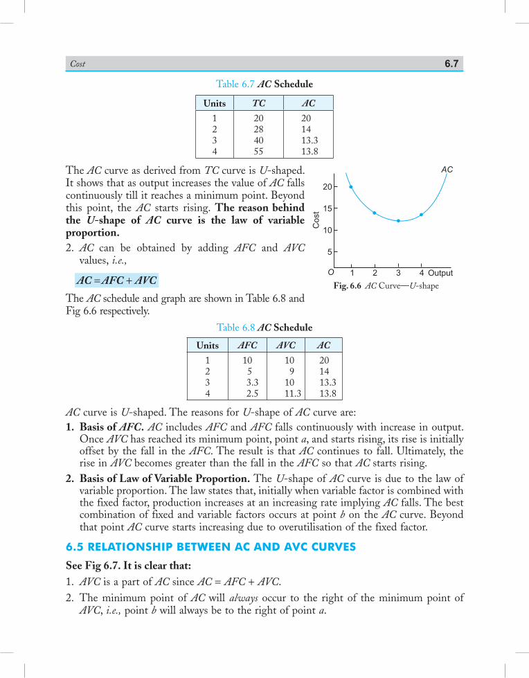
Cost 6.7
Table 6.7 AC Schedule
Units TC AC
1234
20284055
201413.313.8
The AC curve as derived from TC curve is U-shaped. It shows that as output increases the value of AC falls continuously till it reaches a minimum point. Beyond this point, the AC starts rising. The reason behind the U-shape of AC curve is the law of variable proportion.2. AC can be obtained by adding AFC and AVC
values, i.e.,
AC = AFC + AVC
The AC schedule and graph are shown in Table 6.8 and Fig 6.6 respectively.
Table 6.8 AC Schedule
Units AFC AVC AC
1234
1053.32.5
109
1011.3
201413.313.8
AC curve is U-shaped. The reasons for U-shape of AC curve are:1. Basis of AFC. AC includes AFC and AFC falls continuously with increase in output.
Once AVC has reached its minimum point, point a, and starts rising, its rise is initially offset by the fall in the AFC. The result is that AC continues to fall. Ultimately, the rise in AVC becomes greater than the fall in the AFC so that AC starts rising.
2. Basis of Law of Variable Proportion. The U-shape of AC curve is due to the law of variable proportion. The law states that, initially when variable factor is combined with the fixed factor, production increases at an increasing rate implying AC falls. The best combination of fixed and variable factors occurs at point b on the AC curve. Beyond that point AC curve starts increasing due to overutilisation of the fixed factor.
6.5 relationship between aC and aVC CurVes
See Fig 6.7. It is clear that:1. AVC is a part of AC since AC = AFC + AVC.2. The minimum point of AC will always occur to the right of the minimum point of
AVC, i.e., point b will always be to the right of point a.
O
AC
Cost
Output1 2 3 4
20
15
10
5
Fig. 6.6 AC Curve—U-shape
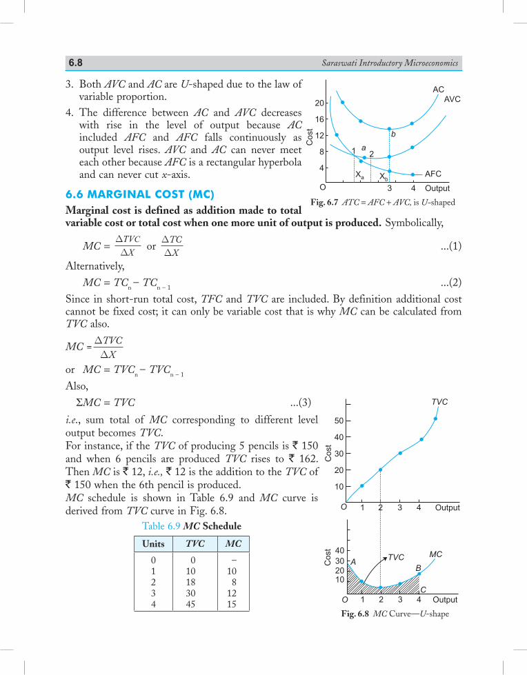
Saraswati Introductory Microeconomics6.8
3. Both AVC and AC are U-shaped due to the law of variable proportion.
4. The difference between AC and AVC decreases with rise in the level of output because AC included AFC and AFC falls continuously as output level rises. AVC and AC can never meet each other because AFC is a rectangular hyperbola and can never cut x-axis.
6.6 Marginal Cost (MC)Marginal cost is defined as addition made to total variable cost or total cost when one more unit of output is produced. Symbolically,
MC = DDTVXC
or DD
TCX
...(1)
Alternatively, MC = TCn – TCn – 1 ...(2)Since in short-run total cost, TFC and TVC are included. By definition additional cost cannot be fixed cost; it can only be variable cost that is why MC can be calculated from TVC also.
MC = DDTVC
X
or MC = TVCn – TVCn – 1
Also, ΣMC = TVC ...(3)
i.e., sum total of MC corresponding to different level output becomes TVC.For instance, if the TVC of producing 5 pencils is ` 150 and when 6 pencils are produced TVC rises to ` 162. Then MC is ` 12, i.e., ` 12 is the addition to the TVC of ` 150 when the 6th pencil is produced.MC schedule is shown in Table 6.9 and MC curve is derived from TVC curve in Fig. 6.8.
Table 6.9 MC Schedule
Units TVC MC
01234
010183045
–108
1215
O
AFC
AC
AVC
Cost
Output
a
b
20
16
12
8
4
1 2
3 4
Xa Xb
Fig. 6.7 ATC = AFC + AVC, is U-shaped
O Output
TVC
Cos
tC
ost
C
40302010
50
40
30
20
10
1 2 3 4
BA TVC MC
O Output1 2 3 4
Fig. 6.8 MC Curve—U-shape
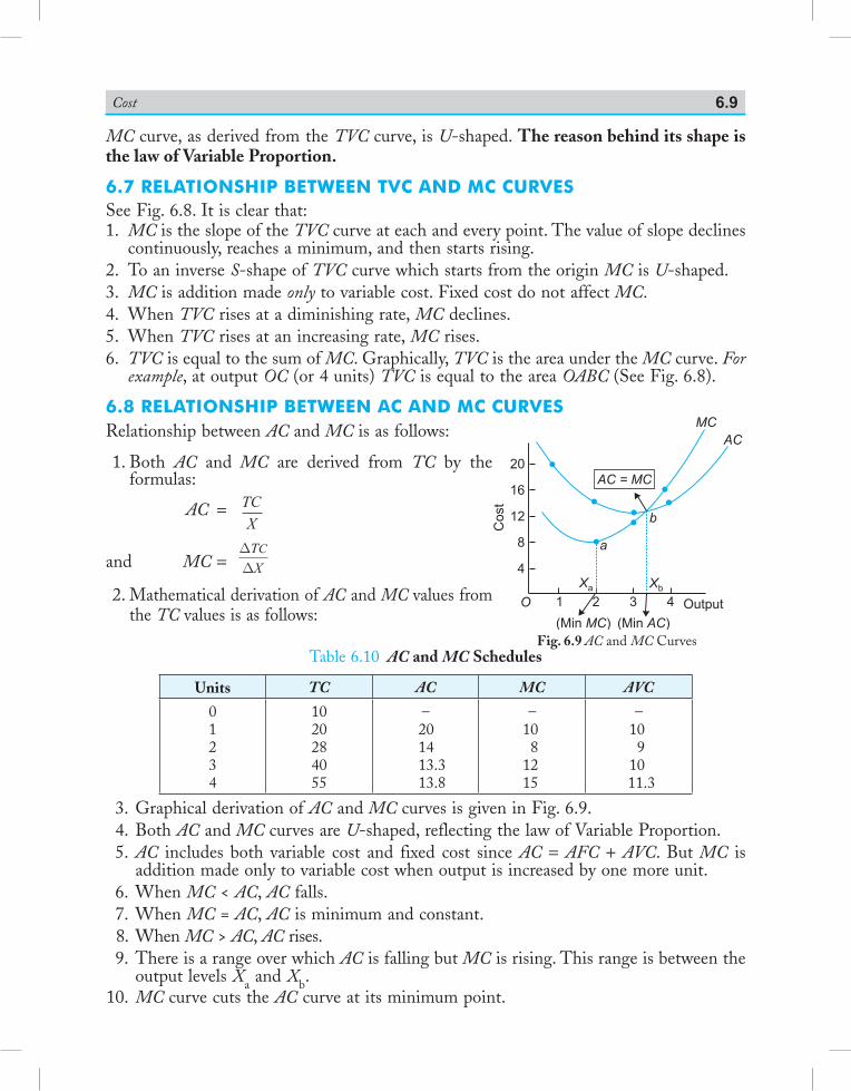
Cost 6.9
MC curve, as derived from the TVC curve, is U-shaped. The reason behind its shape is the law of Variable Proportion.
6.7 relationship between tVC and MC CurVesSee Fig. 6.8. It is clear that:1. MC is the slope of the TVC curve at each and every point. The value of slope declines
continuously, reaches a minimum, and then starts rising.2. To an inverse S-shape of TVC curve which starts from the origin MC is U-shaped.3. MC is addition made only to variable cost. Fixed cost do not affect MC.4. When TVC rises at a diminishing rate, MC declines.5. When TVC rises at an increasing rate, MC rises.6. TVC is equal to the sum of MC. Graphically, TVC is the area under the MC curve. For
example, at output OC (or 4 units) TVC is equal to the area OABC (See Fig. 6.8).
6.8 relationship between aC and MC CurVesRelationship between AC and MC is as follows:
1. Both AC and MC are derived from TC by the formulas:
AC = TCX
and MC = DDTXC
2. Mathematical derivation of AC and MC values from the TC values is as follows:
Table 6.10 AC and MC Schedules
Units TC AC MC AVC
01234
1020284055
–201413.313.8
–108
1215
–109
1011.3
3. Graphical derivation of AC and MC curves is given in Fig. 6.9. 4. Both AC and MC curves are U-shaped, reflecting the law of Variable Proportion. 5. AC includes both variable cost and fixed cost since AC = AFC + AVC. But MC is
addition made only to variable cost when output is increased by one more unit. 6. When MC < AC, AC falls. 7. When MC = AC, AC is minimum and constant. 8. When MC > AC, AC rises. 9. There is a range over which AC is falling but MC is rising. This range is between the
output levels Xa and Xb. 10. MC curve cuts the AC curve at its minimum point.
O
MC
AC
Cost
(Min )MC (Min )AC
Output
AC = MC
20
16
12
8
4
1 2 3 4
a
b
Xa
Xb
Fig. 6.9 AC and MC Curves
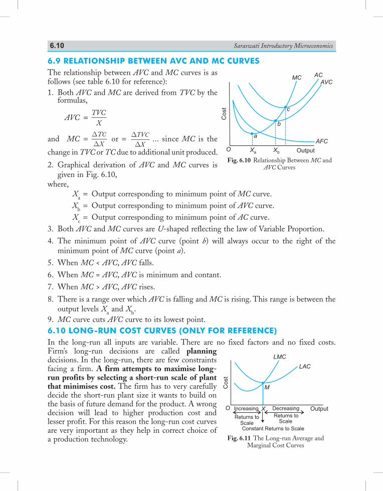
Saraswati Introductory Microeconomics6.10
6.9 relationship between aVC and MC CurVesThe relationship between AVC and MC curves is as follows (see table 6.10 for reference):1. Both AVC and MC are derived from TVC by the
formulas,
AVC = TVC
X
and MC = DD
TXC
or = DDTVXC ... since MC is the
change in TVC or TC due to additional unit produced.
2. Graphical derivation of AVC and MC curves is given in Fig. 6.10,
where, Xa = Output corresponding to minimum point of MC curve. Xb = Output corresponding to minimum point of AVC curve. Xc = Output corresponding to minimum point of AC curve.3. Both AVC and MC curves are U-shaped reflecting the law of Variable Proportion.
4. The minimum point of AVC curve (point b) will always occur to the right of the minimum point of MC curve (point a).
5. When MC < AVC, AVC falls.
6. When MC = AVC, AVC is minimum and contant.
7. When MC > AVC, AVC rises.
8. There is a range over which AVC is falling and MC is rising. This range is between the output levels Xa and Xb.
9. MC curve cuts AVC curve to its lowest point.6.10 long-run Cost CurVes (only for referenCe)In the long-run all inputs are variable. There are no fixed factors and no fixed costs. Firm’s long-run decisions are called planning decisions. In the long-run, there are few constraints facing a firm. A firm attempts to maximise long-run profits by selecting a short-run scale of plant that minimises cost. The firm has to very carefully decide the short-run plant size it wants to build on the basis of future demand for the product. A wrong decision will lead to higher production cost and lesser profit. For this reason the long-run cost curves are very important as they help in correct choice of a production technology.
O
AVC
AFC
Cost
Output
MCAC
a
b
c
Xa
Xb
Fig. 6.10 Relationship Between MC and AVC Curves
O X
LAC
LMC
Cos
t
Output
M
Fig. 6.11 The Long-run Average and Marginal Cost Curves
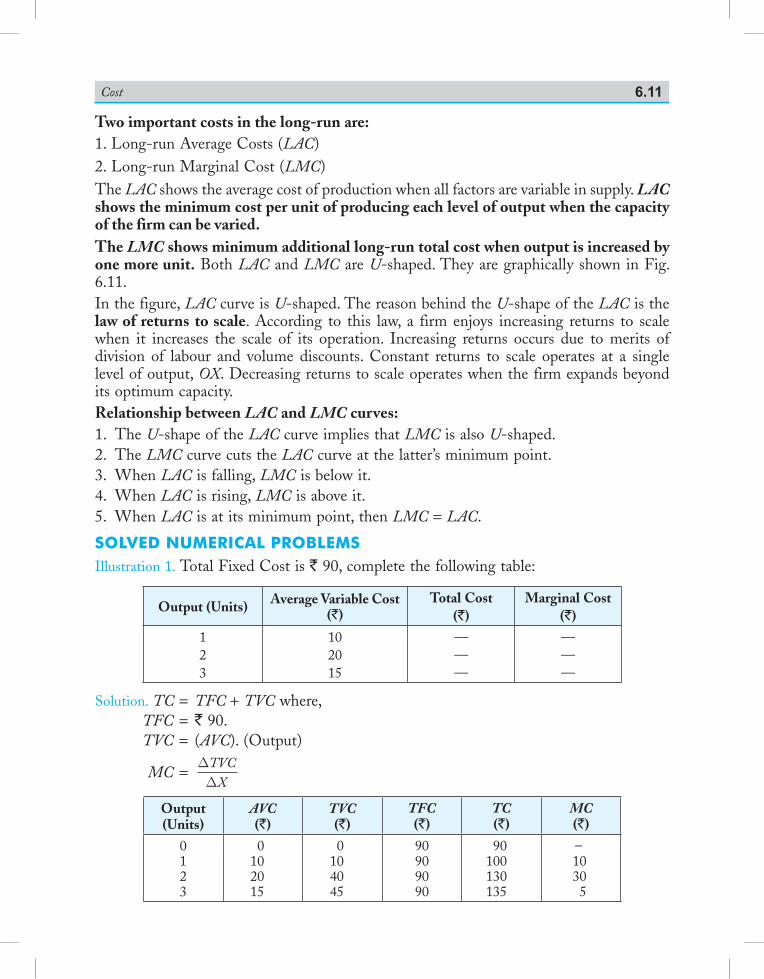
Cost 6.11
Two important costs in the long-run are:1. Long-run Average Costs (LAC)2. Long-run Marginal Cost (LMC)The LAC shows the average cost of production when all factors are variable in supply. LAC shows the minimum cost per unit of producing each level of output when the capacity of the firm can be varied.The LMC shows minimum additional long-run total cost when output is increased by one more unit. Both LAC and LMC are U-shaped. They are graphically shown in Fig. 6.11.In the figure, LAC curve is U-shaped. The reason behind the U-shape of the LAC is the law of returns to scale. According to this law, a firm enjoys increasing returns to scale when it increases the scale of its operation. Increasing returns occurs due to merits of division of labour and volume discounts. Constant returns to scale operates at a single level of output, OX. Decreasing returns to scale operates when the firm expands beyond its optimum capacity.Relationship between LAC and LMC curves:1. The U-shape of the LAC curve implies that LMC is also U-shaped.2. The LMC curve cuts the LAC curve at the latter’s minimum point.3. When LAC is falling, LMC is below it.4. When LAC is rising, LMC is above it.5. When LAC is at its minimum point, then LMC = LAC.
solVed nuMeriCal probleMsIllustration 1. Total Fixed Cost is ` 90, complete the following table:
Output (Units) Average Variable Cost (`)
Total Cost(`)
Marginal Cost(`)
123
102015
———
———
Solution. TC = TFC + TVC where, TFC = ` 90. TVC = (AVC). (Output)
MC = DDTVC
X
Output(Units)
AVC(`)
TVC(`)
TFC(`)
TC(`)
MC(`)
0123
0102015
0104045
90909090
90100130135
–10305
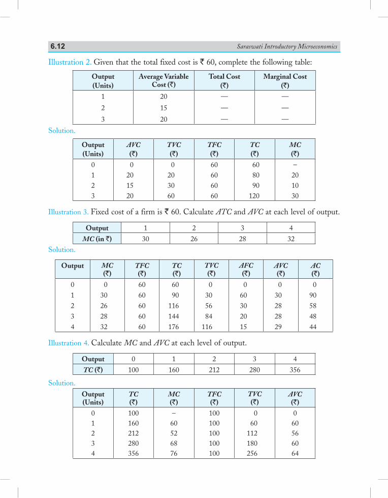
Saraswati Introductory Microeconomics6.12
Illustration 2. Given that the total fixed cost is ` 60, complete the following table:
Output(Units)
Average Variable Cost (`)
Total Cost(`)
Marginal Cost (`)
1
2
3
20
15
20
—
—
—
—
—
—
Solution.
Output(Units)
AVC(`)
TVC(`)
TFC(`)
TC(`)
MC(`)
0123
0201520
0203060
60606060
608090
120
–201030
Illustration 3. Fixed cost of a firm is ` 60. Calculate ATC and AVC at each level of output.
Output 1 2 3 4
MC (in `) 30 26 28 32
Solution.
Output MC(`)
TFC(`)
TC(`)
TVC(`)
AFC(`)
AVC(`)
AC(`)
01234
030262832
6060606060
6090
116144176
0305684
116
060302015
030282829
090584844
Illustration 4. Calculate MC and AVC at each level of output.
Output 0 1 2 3 4
TC (`) 100 160 212 280 356
Solution.Output(Units)
TC(`)
MC(`)
TFC(`)
TVC(`)
AVC(`)
01234
100160212280356
–60526876
100100100100100
060
112180256
060566064
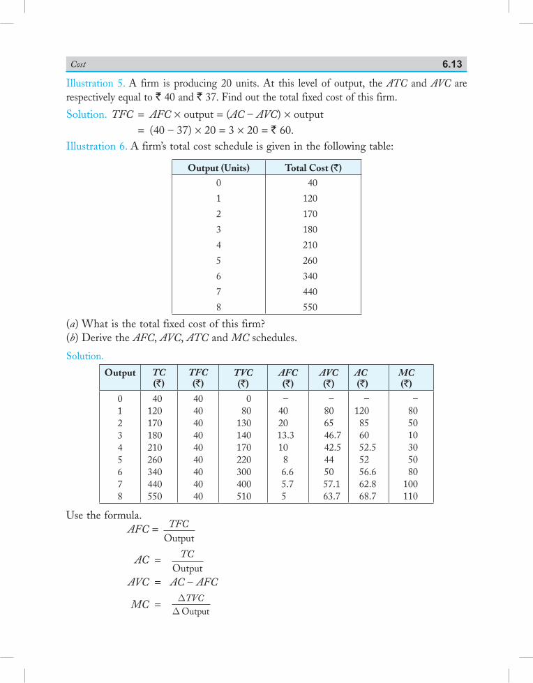
Cost 6.13
Illustration 5. A firm is producing 20 units. At this level of output, the ATC and AVC are respectively equal to ` 40 and ` 37. Find out the total fixed cost of this firm.
Solution. TFC = AFC × output = (AC – AVC) × output = (40 – 37) × 20 = 3 × 20 = ` 60.Illustration 6. A firm’s total cost schedule is given in the following table:
Output (Units) Total Cost (`)
0
1
2
3
4
5
6
7
8
40
120
170
180
210
260
340
440
550
(a) What is the total fixed cost of this firm?(b) Derive the AFC, AVC, ATC and MC schedules.
Solution.
Output TC(`)
TFC(`)
TVC (`)
AFC(`)
AVC(`)
AC(`)
MC(`)
012345678
40120170180210260340440550
404040404040404040
080
130140170220300400510
–402013.3108
6.6 5.7 5
–806546.742.5445057.163.7
–120856052.55256.662.868.7
–805010305080
100110
Use the formula. AFC = TFC
Output
AC = TCOutput
AVC = AC – AFC
MC = D
DTVC
Output
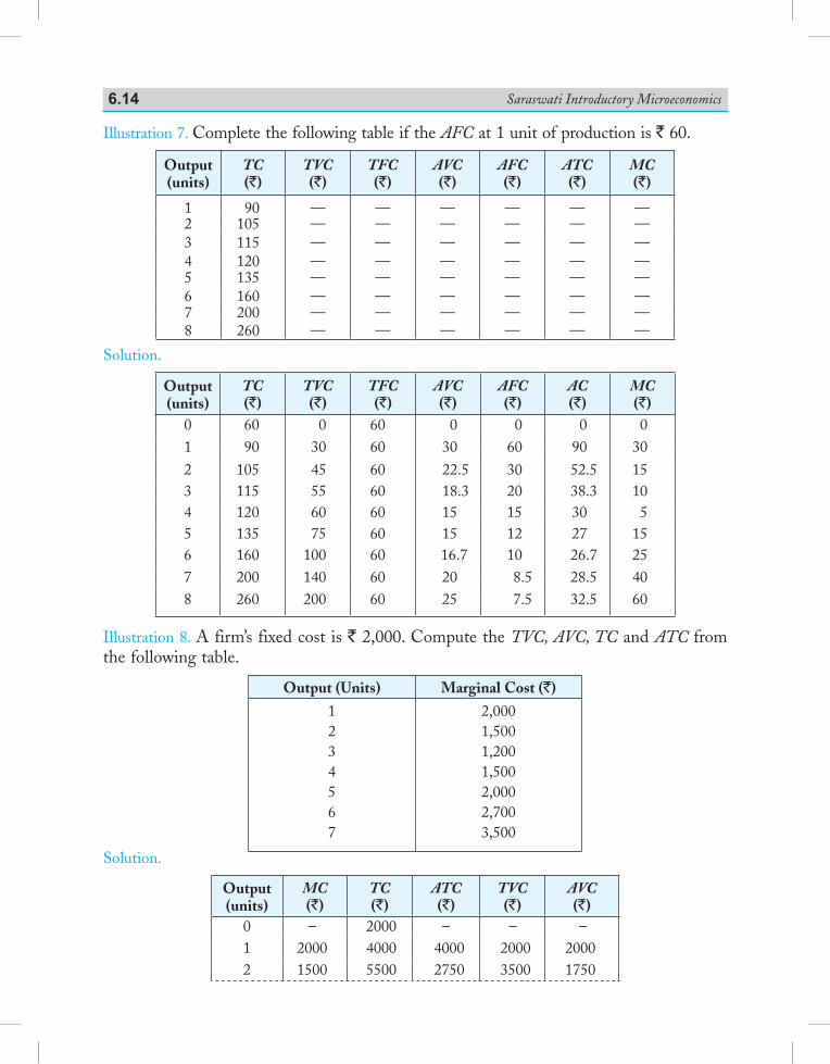
Saraswati Introductory Microeconomics6.14
Illustration 7. Complete the following table if the AFC at 1 unit of production is ` 60.
Output(units)
TC(`)
TVC(`)
TFC(`)
AVC(`)
AFC(`)
ATC(`)
MC(`)
1 90 — — — — — —2 105 — — — — — —3 115 — — — — — —4 120 — — — — — —5 135 — — — — — —6 160 — — — — — —7 200 — — — — — —8 260 — — — — — —
Solution.
Output(units)
TC(`)
TVC(`)
TFC(`)
AVC(`)
AFC(`)
AC(`)
MC(`)
0 60 0 60 0 0 0 01 90 30 60 30 60 90 302 105 45 60 22.5 30 52.5 153 115 55 60 18.3 20 38.3 104 120 60 60 15 15 30 55 135 75 60 15 12 27 156 160 100 60 16.7 10 26.7 257 200 140 60 20 8.5 28.5 408 260 200 60 25 7.5 32.5 60
Illustration 8. A firm’s fixed cost is ` 2,000. Compute the TVC, AVC, TC and ATC from the following table.
Output (Units) Marginal Cost (`)
1234567
2,0001,5001,2001,5002,0002,7003,500
Solution.
Output(units)
MC(`)
TC(`)
ATC(`)
TVC(`)
AVC(`)
0 – 2000 – – –1 2000 4000 4000 2000 20002 1500 5500 2750 3500 1750
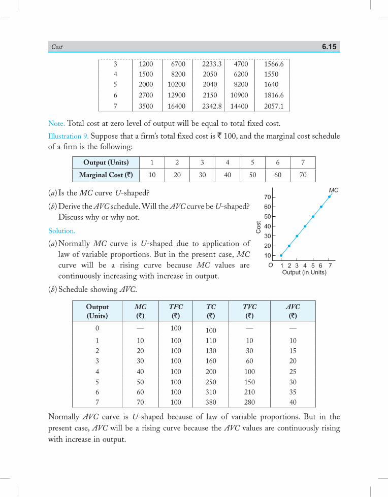
Cost 6.15
3 1200 6700 2233.3 4700 1566.64 1500 8200 2050 6200 15505 2000 10200 2040 8200 1640
6 2700 12900 2150 10900 1816.6
7 3500 16400 2342.8 14400 2057.1
Note. Total cost at zero level of output will be equal to total fixed cost.
Illustration 9. Suppose that a firm’s total fixed cost is ` 100, and the marginal cost schedule of a firm is the following:
Output (Units) 1 2 3 4 5 6 7
Marginal Cost (`) 10 20 30 40 50 60 70
(a) Is the MC curve U-shaped?
(b) Derive the AVC schedule. Will the AVC curve be U-shaped? Discuss why or why not.
Solution.
(a) Normally MC curve is U-shaped due to application of law of variable proportions. But in the present case, MC curve will be a rising curve because MC values are continuously increasing with increase in output.
(b) Schedule showing AVC.
Output (Units)
MC (`)
TFC (`)
TC (`)
TVC (`)
AVC (`)
0 — 100 100 — —
1 10 100 110 10 102 20 100 130 30 153 30 100 160 60 20
4 40 100 200 100 255 50 100 250 150 306 60 100 310 210 357 70 100 380 280 40
Normally AVC curve is U-shaped because of law of variable proportions. But in the present case, AVC will be a rising curve because the AVC values are continuously rising with increase in output.
O
MC
Cost
Output (in Units)
70
60
50
40
20
30
10
1 2 3 4 5 6 7
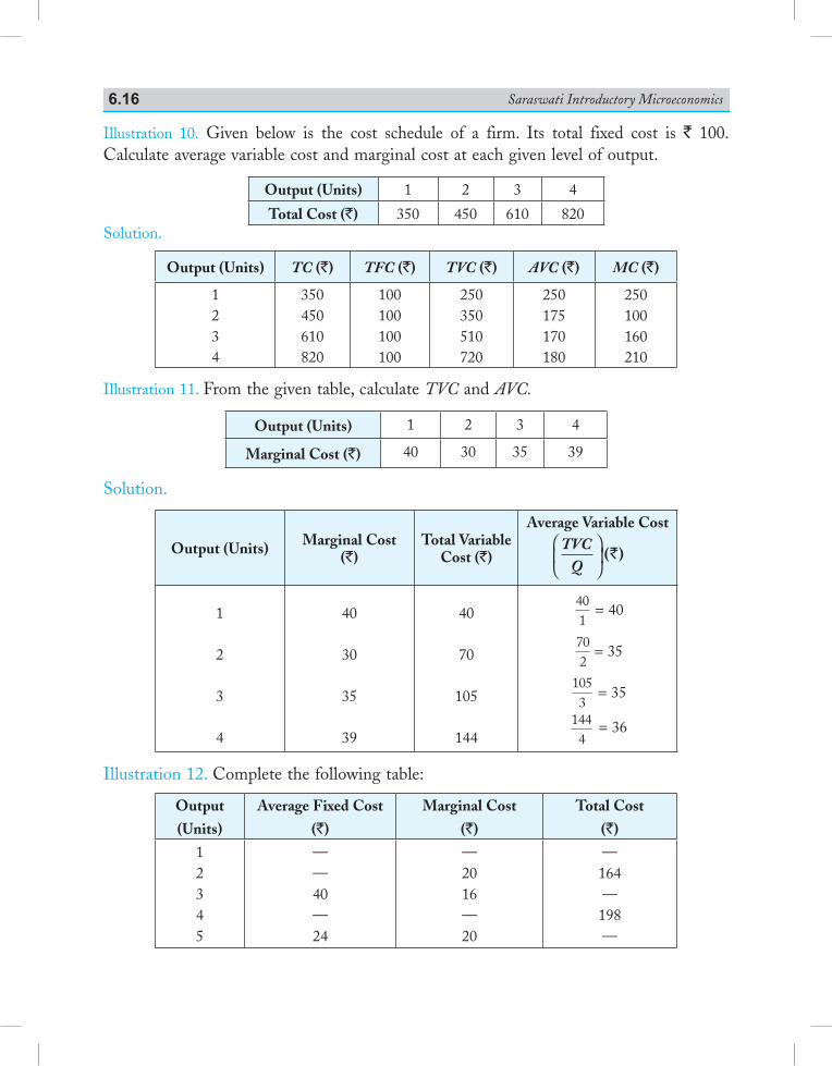
Saraswati Introductory Microeconomics6.16
Illustration 10. Given below is the cost schedule of a firm. Its total fixed cost is ` 100. Calculate average variable cost and marginal cost at each given level of output.
Output (Units) 1 2 3 4
Total Cost (`) 350 450 610 820Solution.
Output (Units) TC (`) TFC (`) TVC (`) AVC (`) MC (`)
1234
350450610820
100100100100
250350510720
250175170180
250100160210
Illustration 11. From the given table, calculate TVC and AVC.
Output (Units) 1 2 3 4
Marginal Cost (`) 40 30 35 39
Solution.
Output (Units) Marginal Cost (`)
Total Variable Cost (`)
Average Variable CostTVCQ
( )`
1
2
3
4
40
30
35
39
40
70
105
144
401
= 40
702
= 35
1053
= 35
1444
= 36
Illustration 12. Complete the following table:
Output (Units)
Average Fixed Cost(`)
Marginal Cost (`)
Total Cost (`)
12345
——40—24
—2016—20
—164—198—
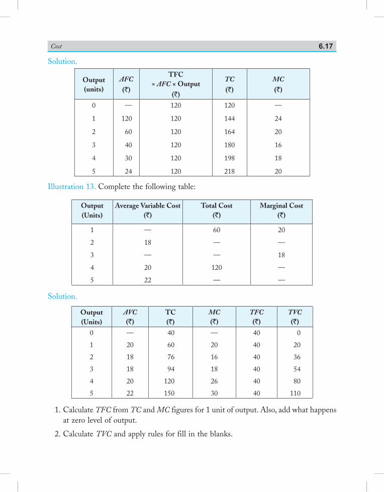
Cost 6.17
Solution.
Output(units)
AFC
(`)
TFC = AFC × Output
(`)
TC
(`)MC
(`)
0
1
2
3
4
5
—
120
60
40
30
24
120
120
120
120
120
120
120
144
164
180
198
218
—
24
20
16
18
20
Illustration 13. Complete the following table:
Output (Units)
Average Variable Cost (`)
Total Cost (`)
Marginal Cost(`)
1
2
3
4
5
—
18
—
20
22
60
—
—
120
—
20
—
18
—
—
Solution.
Output(Units)
AVC(`)
TC(`)
MC(`)
TFC(`)
TVC(`)
0
1
2
3
4
5
—
20
18
18
20
22
40
60
76
94
120
150
—
20
16
18
26
30
40
40
40
40
40
40
0
20
36
54
80
110
1. Calculate TFC from TC and MC figures for 1 unit of output. Also, add what happens at zero level of output.
2. Calculate TVC and apply rules for fill in the blanks.
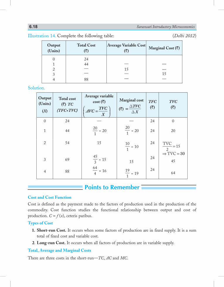
Saraswati Introductory Microeconomics6.18
Illustration 14. Complete the following table: (Delhi 2012)
Output (Units)
Total Cost (`)
Average Variable Cost (`)
Marginal Cost (`)
01234
2444——
88
—15——
——15—
Solution.
Output (Units)
(X)
Total cost (`) TC
(TFC+TVC)
Average variable cost (`)
AVC TVCX
=
Marginal cost
(`) =DDTVCX
TFC(`)
TVC(`)
0
1
24
44
—
201
= 20
—
201
= 20
24
24
0
20
2
3
4
54
69
88
15
453
= 15
644
= 16
101
= 10
15
191
= 19
24
24
24
TVC
TVC2
15=
=⇒ 30
45
64
Points to RememberCost and Cost Function
Cost is defined as the payment made to the factors of production used in the production of the commodity. Cost function studies the functional relationship between output and cost of pro duc tion. C = f (x), ceteris paribus.
Types of Cost
1. Short-run Cost. It occurs when some factors of production are in fixed supply. It is a sum total of fixed cost and variable cost.
2. Long-run Cost. It occurs when all factors of production are in variable supply.
Total, Average and Marginal Costs
There are three costs in the short-run—TC, AC and MC.
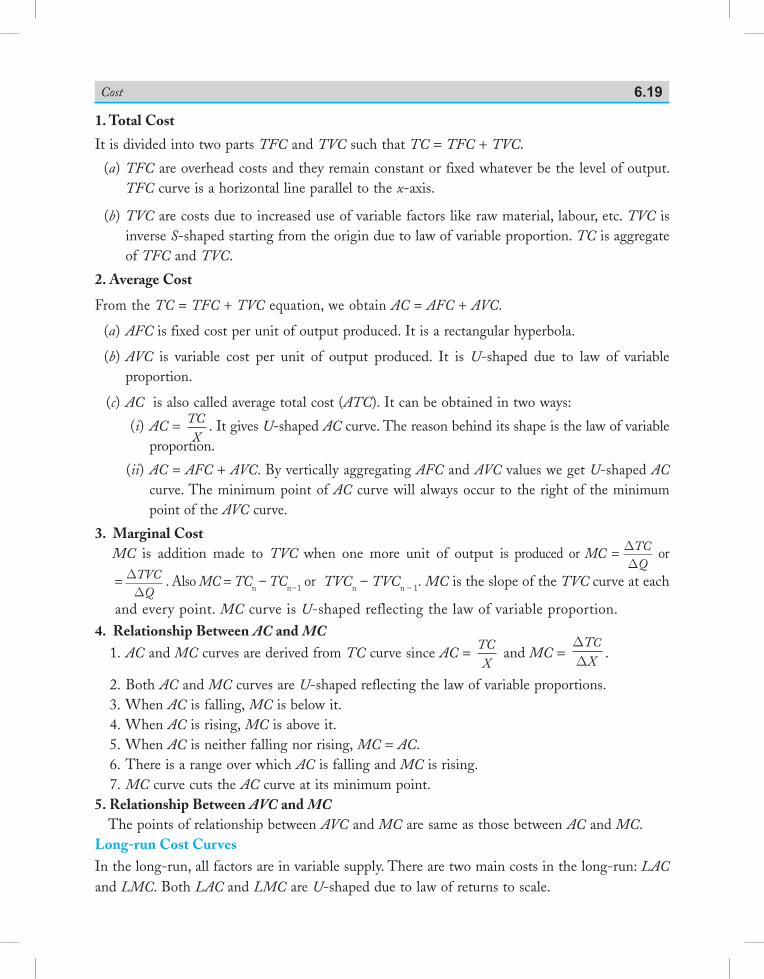
Cost 6.19
1. Total Cost
It is divided into two parts TFC and TVC such that TC = TFC + TVC.
(a) TFC are overhead costs and they remain constant or fixed whatever be the level of output. TFC curve is a horizontal line parallel to the x-axis.
(b) TVC are costs due to increased use of variable factors like raw material, labour, etc. TVC is inverse S-shaped starting from the origin due to law of variable proportion. TC is aggregate of TFC and TVC.
2. Average Cost
From the TC = TFC + TVC equation, we obtain AC = AFC + AVC.
(a) AFC is fixed cost per unit of output produced. It is a rectangular hyperbola.
(b) AVC is variable cost per unit of output produced. It is U-shaped due to law of variable proportion.
(c) AC is also called average total cost (ATC). It can be obtained in two ways:
(i) AC = TCX
. It gives U-shaped AC curve. The reason behind its shape is the law of variable proportion.
(ii) AC = AFC + AVC. By vertically aggregating AFC and AVC values we get U-shaped AC curve. The minimum point of AC curve will always occur to the right of the minimum point of the AVC curve.
3. Marginal Cost MC is addition made to TVC when one more unit of output is produced or MC = D
DTCQ
or
= DDTVC
Q. Also MC = TCn – TCn – 1 or TVCn – TVCn – 1. MC is the slope of the TVC curve at each
and every point. MC curve is U-shaped reflecting the law of variable proportion.4. Relationship Between AC and MC 1. AC and MC curves are derived from TC curve since AC = TC
X and MC =
DD
TXC
.
2. Both AC and MC curves are U-shaped reflecting the law of variable proportions. 3. When AC is falling, MC is below it. 4. When AC is rising, MC is above it. 5. When AC is neither falling nor rising, MC = AC. 6. There is a range over which AC is falling and MC is rising. 7. MC curve cuts the AC curve at its minimum point.5. Relationship Between AVC and MC The points of relationship between AVC and MC are same as those between AC and MC.Long-run Cost CurvesIn the long-run, all factors are in variable supply. There are two main costs in the long-run: LAC and LMC. Both LAC and LMC are U-shaped due to law of returns to scale.
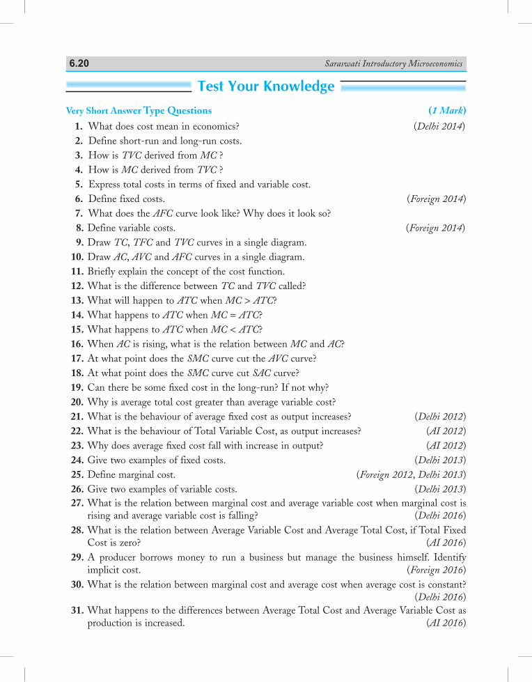
Saraswati Introductory Microeconomics6.20
Test Your KnowledgeVery Short Answer Type Questions (1 Mark)
1. What does cost mean in economics? (Delhi 2014) 2. Define short-run and long-run costs. 3. How is TVC derived from MC ? 4. How is MC derived from TVC ? 5. Express total costs in terms of fixed and variable cost. 6. Define fixed costs. (Foreign 2014) 7. What does the AFC curve look like? Why does it look so? 8. Define variable costs. (Foreign 2014) 9. Draw TC, TFC and TVC curves in a single diagram. 10. Draw AC, AVC and AFC curves in a single diagram. 11. Briefly explain the concept of the cost function. 12. What is the difference between TC and TVC called? 13. What will happen to ATC when MC > ATC? 14. What happens to ATC when MC = ATC? 15. What happens to ATC when MC < ATC? 16. When AC is rising, what is the relation between MC and AC? 17. At what point does the SMC curve cut the AVC curve? 18. At what point does the SMC curve cut SAC curve? 19. Can there be some fi xed cost in the long-run? If not why? 20. Why is average total cost greater than average variable cost? 21. What is the behaviour of average fi xed cost as output increases? (Delhi 2012) 22. What is the behaviour of Total Variable Cost, as output increases? (AI 2012) 23. Why does average fi xed cost fall with increase in output? (AI 2012) 24. Give two examples of fixed costs. (Delhi 2013) 25. Define marginal cost. (Foreign 2012, Delhi 2013) 26. Give two examples of variable costs. (Delhi 2013) 27. What is the relation between marginal cost and average variable cost when marginal cost is
rising and average variable cost is falling? (Delhi 2016) 28. What is the relation between Average Variable Cost and Average Total Cost, if Total Fixed
Cost is zero? (AI 2016) 29. A producer borrows money to run a business but manage the business himself. Identify
implicit cost. (Foreign 2016) 30. What is the relation between marginal cost and average cost when average cost is constant?
(Delhi 2016) 31. What happens to the differences between Average Total Cost and Average Variable Cost as
production is increased. (AI 2016)
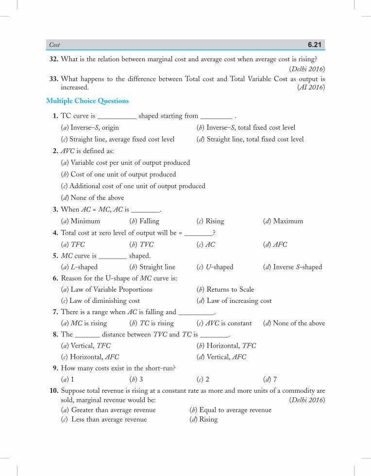
Cost 6.21
32. What is the relation between marginal cost and average cost when average cost is rising? (Delhi 2016) 33. What happens to the difference between Total cost and Total Variable Cost as output is
increased. (AI 2016)
Multiple Choice Questions
1. TC curve is ___________ shaped starting from _________ .
(a) Inverse–S, origin (b) Inverse–S, total fixed cost level
(c) Straight line, average fixed cost level (d) Straight line, total fixed cost level
2. AVC is defined as:
(a) Variable cost per unit of output produced
(b) Cost of one unit of output produced
(c) Additional cost of one unit of output produced
(d) None of the above
3. When AC = MC, AC is ________.
(a) Minimum (b) Falling (c) Rising (d) Maximum
4. Total cost at zero level of output will be = ________?
(a) TFC (b) TVC (c) AC (d) AFC
5. MC curve is ________ shaped.
(a) L-shaped (b) Straight line (c) U-shaped (d) Inverse S-shaped
6. Reason for the U-shape of MC curve is:
(a) Law of Variable Proportions (b) Returns to Scale
(c) Law of diminishing cost (d) Law of increasing cost
7. There is a range when AC is falling and __________.
(a) MC is rising (b) TC is rising (c) AVC is constant (d) None of the above
8. The _______ distance between TVC and TC is ________.
(a) Vertical, TFC (b) Horizontal, TFC
(c) Horizontal, AFC (d) Vertical, AFC
9. How many costs exist in the short-run?
(a) 1 (b) 3 (c) 2 (d) 7
10. Suppose total revenue is rising at a constant rate as more and more units of a commodity are sold, marginal revenue would be: (Delhi 2016)
(a) Greater than average revenue (b) Equal to average revenue (c) Less than average revenue (d) Rising
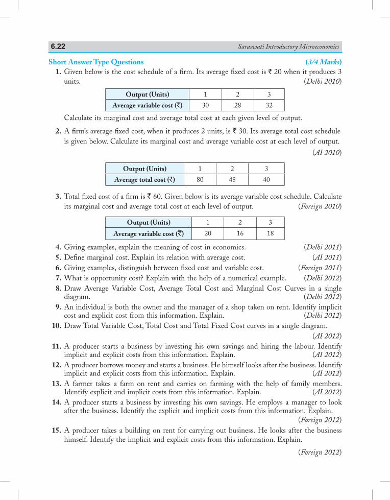
Saraswati Introductory Microeconomics6.22
Short Answer Type Questions (3/4 Marks) 1. Given below is the cost schedule of a firm. Its average fixed cost is ` 20 when it produces 3
units. (Delhi 2010)
Output (Units) 1 2 3
Average variable cost (`) 30 28 32
Calculate its marginal cost and average total cost at each given level of output.
2. A firm’s average fixed cost, when it produces 2 units, is ` 30. Its average total cost schedule is given below. Calculate its marginal cost and average variable cost at each level of output.
(AI 2010)
Output (Units) 1 2 3
Average total cost (`) 80 48 40
3. Total fixed cost of a firm is ` 60. Given below is its average variable cost schedule. Calculate its marginal cost and average total cost at each level of output. (Foreign 2010)
Output (Units) 1 2 3
Average variable cost (`) 20 16 18
4. Giving examples, explain the meaning of cost in economics. (Delhi 2011) 5. Define marginal cost. Explain its relation with average cost. (AI 2011) 6. Giving examples, distinguish between fixed cost and variable cost. (Foreign 2011) 7. What is opportunity cost? Explain with the help of a numerical example. (Delhi 2012) 8. Draw Average Variable Cost, Average Total Cost and Marginal Cost Curves in a single
diagram. (Delhi 2012) 9. An individual is both the owner and the manager of a shop taken on rent. Identify implicit
cost and explicit cost from this information. Explain. (Delhi 2012) 10. Draw Total Variable Cost, Total Cost and Total Fixed Cost curves in a single diagram.
(AI 2012) 11. A producer starts a business by investing his own savings and hiring the labour. Identify
implicit and explicit costs from this information. Explain. (AI 2012) 12. A producer borrows money and starts a business. He himself looks after the business. Identify
implicit and explicit costs from this information. Explain. (AI 2012) 13. A farmer takes a farm on rent and carries on farming with the help of family members.
Identify explicit and implicit costs from this information. Explain. (AI 2012) 14. A producer starts a business by investing his own savings. He employs a manager to look
after the business. Identify the explicit and implicit costs from this information. Explain. (Foreign 2012) 15. A producer takes a building on rent for carrying out business. He looks after the business
himself. Identify the implicit and explicit costs from this information. Explain.
(Foreign 2012)
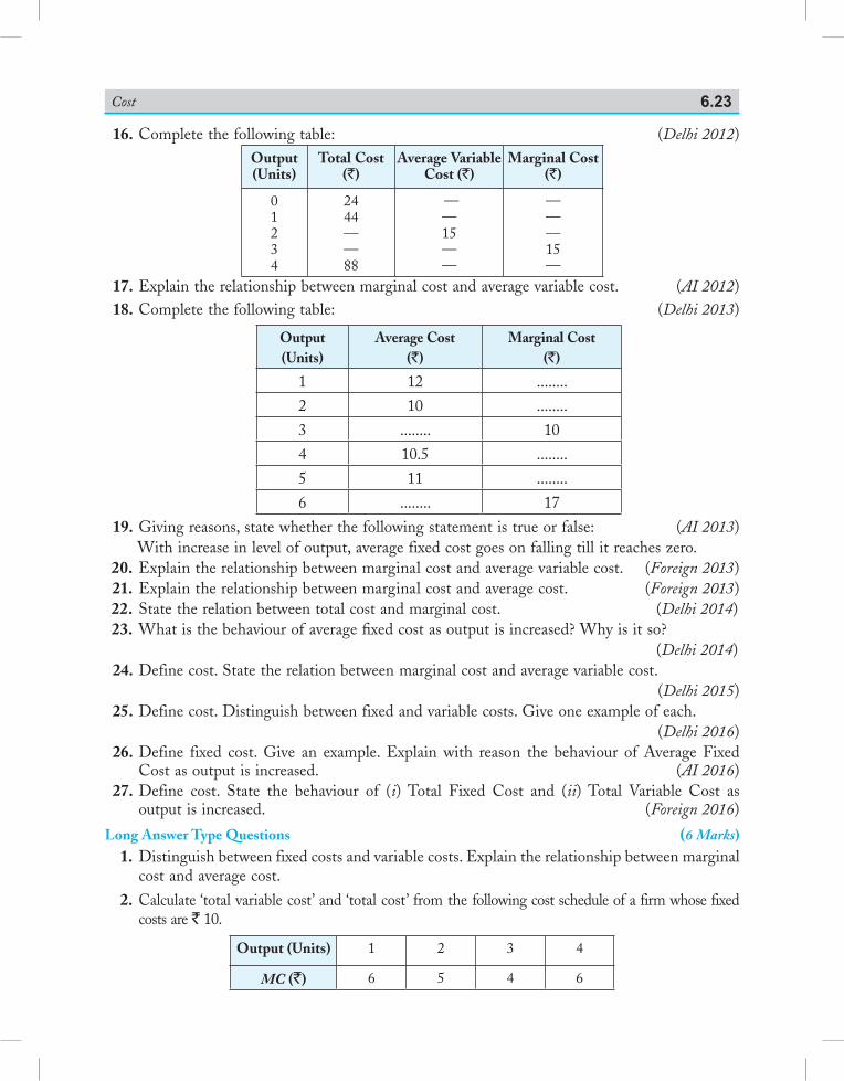
Cost 6.23
16. Complete the following table: (Delhi 2012)Output (Units)
Total Cost (`)
Average Variable Cost (`)
Marginal Cost (`)
01234
2444——88
——15——
———15—
17. Explain the relationship between marginal cost and average variable cost. (AI 2012) 18. Complete the following table: (Delhi 2013)
Output(Units)
Average Cost(`)
Marginal Cost(`)
1 12 ........2 10 ........3 ........ 104 10.5 ........5 11 ........6 ........ 17
19. Giving reasons, state whether the following statement is true or false: (AI 2013) With increase in level of output, average fixed cost goes on falling till it reaches zero. 20. Explain the relationship between marginal cost and average variable cost. (Foreign 2013) 21. Explain the relationship between marginal cost and average cost. (Foreign 2013) 22. State the relation between total cost and marginal cost. (Delhi 2014) 23. What is the behaviour of average fixed cost as output is increased? Why is it so? (Delhi 2014) 24. Define cost. State the relation between marginal cost and average variable cost. (Delhi 2015) 25. Define cost. Distinguish between fixed and variable costs. Give one example of each. (Delhi 2016) 26. Define fixed cost. Give an example. Explain with reason the behaviour of Average Fixed
Cost as output is increased. (AI 2016) 27. Define cost. State the behaviour of (i) Total Fixed Cost and (ii) Total Variable Cost as
output is increased. (Foreign 2016)
Long Answer Type Questions (6 Marks) 1. Distinguish between fixed costs and variable costs. Explain the relationship between marginal
cost and average cost.
2. Calculate ‘total variable cost’ and ‘total cost’ from the following cost schedule of a firm whose fixed costs are ` 10.
Output (Units) 1 2 3 4
MC (`) 6 5 4 6
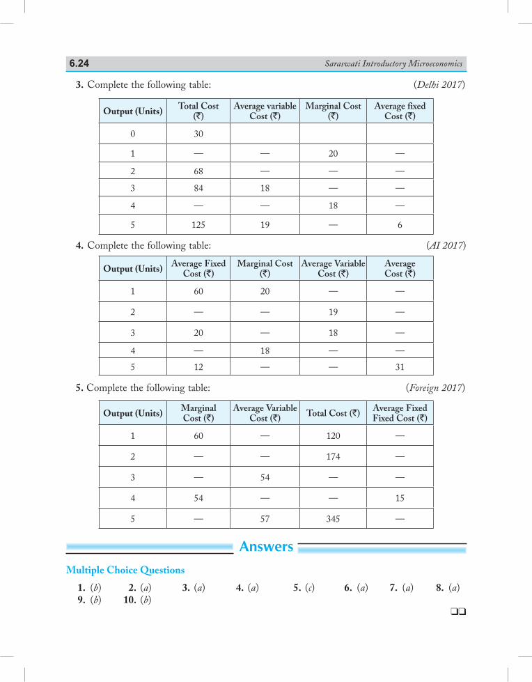
Saraswati Introductory Microeconomics6.24
3. Complete the following table: (Delhi 2017)
Output (Units) Total Cost (`)
Average variable Cost (`)
Marginal Cost (`)
Average fixed Cost (`)
0 30
1 — — 20 —
2 68 — — —
3 84 18 — —
4 — — 18 —
5 125 19 — 6
4. Complete the following table: (AI 2017)
Output (Units) Average Fixed Cost (`)
Marginal Cost (`)
Average Variable Cost (`)
Average Cost (`)
1 60 20 — —
2 — — 19 —
3 20 — 18 —
4 — 18 — —
5 12 — — 31
5. Complete the following table: (Foreign 2017)
Output (Units) Marginal Cost (`)
Average Variable Cost (`) Total Cost (`) Average Fixed
Fixed Cost (`)
1 60 — 120 —
2 — — 174 —
3 — 54 — —
4 54 — — 15
5 — 57 345 —
AnswersMultiple Choice Questions
1. (b) 2. (a) 3. (a) 4. (a) 5. (c) 6. (a) 7. (a) 8. (a) 9. (b) 10. (b)
7.1 meaning of revenue
Revenue is the money payment received from the sale of a commodity. The terms mostly used with revenue are: Total Revenue, Average Revenue and Marginal Revenue.
7.2 Types of revenue
7.2.1 Total Revenue (TR)TR is defined as the total or aggregate of proceeds to the firm from the sale of a commodity. It is calculated by multiplying price (P) by the quantity sold (Q). For example, if a firm sells 5 chairs at the price of ` 100 per chair, the total revenue will be equal to 5 × 100 = ` 500Symbolically,
TR = P.Qwhere P = Price Q = Quantity sold
7.2.2 Average Revenue (AR)AR is revenue per unit of output sold. It is obtained by dividing total revenue by the number of units sold. For example, if the TR of a firm from sale of 5 chairs is ` 500, then
AR will be equal to 5005
= ` 100.Symbolically,
AR = Total Revenue
Number of units sold
Revenue
Chapter Scheme
7
7.1 Meaning of Revenue7.2 Types of Revenue 7.2.1 Total Revenue (TR) 7.2.2 Average Revenue (AR) 7.2.3 Marginal Revenue (MR)7.3 Relationship between TR, AR and MR 7.3.1 Under Perfect Competition 7.3.2 Under Monopoly or Monopolistic
Competition7.4 Relationship between TR and MR
7.5 Relationship between AR and MR7.6 Relationship between TR, AR and MR
Curves Under Both Perfect and Monopolistic Competitions
7.7 Relationship between Revenue and Elasticity of Demand
Solved Numerical Problems Points to Remember Test Your Knowledge
Answers to MCQs
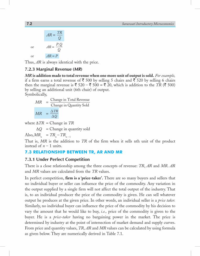
Saraswati Introductory Microeconomics7.2
AR = TRQ
or AR = P.QQ
or AR = P
Thus, AR is always identical with the price.
7.2.3 Marginal Revenue (MR)MR is addition made to total revenue when one more unit of output is sold. For example, if a firm earns a total revenue of ` 500 by selling 5 chairs and ` 520 by selling 6 chairs then the marginal revenue is ` 520 – ` 500 = ` 20, which is addition to the TR (` 500) by selling an additional unit (6th chair) of output.Symbolically,
MR = Change in Total RevenueChange in Quantity Sold
MR = DD
TRQ
where ΔTR = Change in TR ΔQ = Change in quantity soldAlso, MRn = TRn – TRn – 1
That is, MR is the addition to TR of the firm when it sells nth unit of the product instead of n – 1 units.7.3 relaTionship beTween Tr, ar and mr
7.3.1 Under Perfect CompetitionThere is a close relationship among the three concepts of revenue: TR, AR and MR. AR and MR values are calculated from the TR values.
In perfect competition, firm is a ‘price-taker’. There are so many buyers and sellers that no individual buyer or seller can influence the price of the commodity. Any variation in the output supplied by a single firm will not affect the total output of the industry. That is, to an individual producer the price of the commodity is given. He can sell whatever output he produces at the given price. In other words, an individual seller is a price taker. Similarly, no individual buyer can influence the price of the commodity by his decision to vary the amount that he would like to buy, i.e., price of the commodity is given to the buyer. He is a price-taker having no bargaining power in the market. The price is determined by industry at the point of intersection of market demand and supply curves. From price and quantity values, TR, AR and MR values can be calculated by using formula as given below. They are numerically derived in Table 7.1.
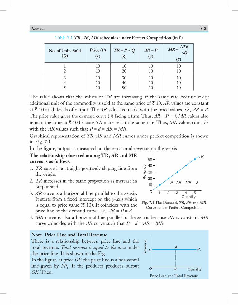
Revenue 7.3
Table 7.1 TR, AR, MR schedules under Perfect Competition (in `)
No. of Units Sold (Q)
Price (P)(`)
TR = P × Q(`)
AR = P(`)
MR = ∆∆TR
Q
(`)
12
1010
1020
1010
1010
345
101010
304050
101010
101010
The table shows that the values of TR are increasing at the same rate because every additional unit of the commodity is sold at the same price of ` 10. AR values are constant at ` 10 at all levels of output. The AR values coincide with the price values, i.e., AR = P. The price value gives the demand curve (d) facing a firm. Thus, AR = P = d. MR values also remain the same at ` 10 because TR increases at the same rate. Thus, MR values coincide with the AR values such that P = d = AR = MR.Graphical representation of TR, AR and MR curves under perfect competition is shown in Fig. 7.1.In the figure, output is measured on the x-axis and revenue on the y-axis. The relationship observed among TR, AR and MR curves is as follows:1. TR curve is a straight positively sloping line from
the origin.2. TR increases in the same proportion as increase in
output sold.3. AR curve is a horizontal line parallel to the x-axis.
It starts from a fixed intercept on the y-axis which is equal to price value (` 10). It coincides with the price line or the demand curve, i.e., AR = P = d.
4. MR curve is also a horizontal line parallel to the x-axis because AR is constant. MR curve coincides with the AR curve such that P = d = AR = MR.
Note. Price Line and Total RevenueThere is a relationship between price line and the total revenue. Total revenue is equal to the area under the price line. It is shown in the Fig.In the figure, at price OP, the price line is a horizontal line given by PP1. If the producer produces output OX. Then:
Fig. 7.1 The Demand, TR, AR and MR Curves under Perfect Competition
Revenue
50
40
30
20
10
O 1 2 3 4 5Quantity
TR
P= AR = MR = d
Price Line and Total Revenue
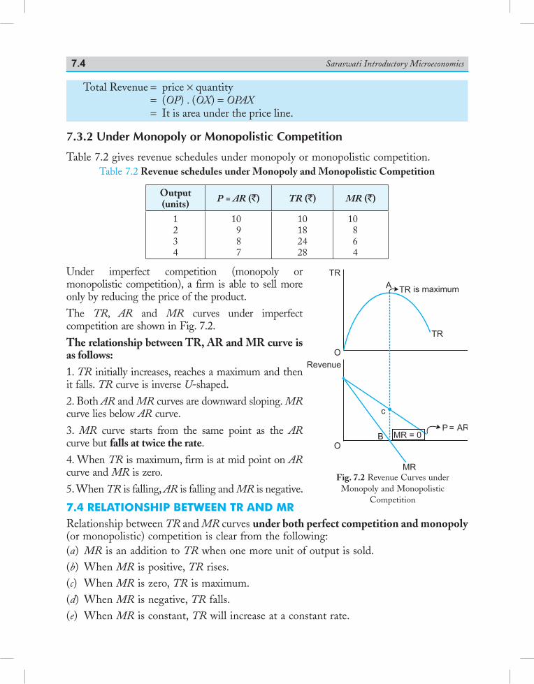
Saraswati Introductory Microeconomics7.4
Total Revenue = price × quantity = (OP) . (OX) = OPAX = It is area under the price line.
7.3.2 Under Monopoly or Monopolistic Competition
Table 7.2 gives revenue schedules under monopoly or monopolistic competition.Table 7.2 Revenue schedules under Monopoly and Monopolistic Competition
Output (units) P = AR (`) TR (`) MR (`)
1234
10987
10182428
10864
Under imperfect competition (monopoly or monopolistic competition), a firm is able to sell more only by reducing the price of the product. The TR, AR and MR curves under imperfect competition are shown in Fig. 7.2.The relationship between TR, AR and MR curve is as follows: 1. TR initially increases, reaches a maximum and then it falls. TR curve is inverse U-shaped. 2. Both AR and MR curves are downward sloping. MR curve lies below AR curve. 3. MR curve starts from the same point as the AR curve but falls at twice the rate.4. When TR is maximum, firm is at mid point on AR curve and MR is zero.5. When TR is falling, AR is falling and MR is negative.
7.4 relaTionship beTween Tr and mrRelationship between TR and MR curves under both perfect competition and monopoly (or monopolistic) competition is clear from the following:(a) MR is an addition to TR when one more unit of output is sold.(b) When MR is positive, TR rises.(c) When MR is zero, TR is maximum.(d) When MR is negative, TR falls.(e) When MR is constant, TR will increase at a constant rate.
Fig. 7.2 Revenue Curves under Monopoly and Monopolistic
Competition
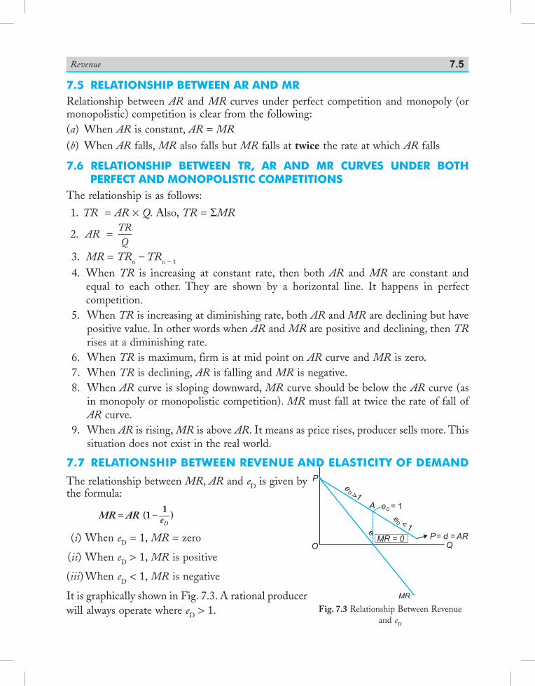
Revenue 7.5
Fig. 7.3 Relationship Between Revenue and eD
7.5 relaTionship beTween ar and mrRelationship between AR and MR curves under perfect competition and monopoly (or monopolistic) competition is clear from the following:(a) When AR is constant, AR = MR(b) When AR falls, MR also falls but MR falls at twice the rate at which AR falls
7.6 relaTionship beTween Tr, ar and mr curves under boTh perfecT and monopolisTic compeTiTions
The relationship is as follows:
1. TR = AR × Q. Also, TR = ΣMR
2. AR = TRQ
3. MR = TRn – TRn – 1
4. When TR is increasing at constant rate, then both AR and MR are constant and equal to each other. They are shown by a horizontal line. It happens in perfect competition.
5. When TR is increasing at diminishing rate, both AR and MR are declining but have positive value. In other words when AR and MR are positive and declining, then TR rises at a diminishing rate.
6. When TR is maximum, firm is at mid point on AR curve and MR is zero. 7. When TR is declining, AR is falling and MR is negative. 8. When AR curve is sloping downward, MR curve should be below the AR curve (as
in monopoly or monopolistic competition). MR must fall at twice the rate of fall of AR curve.
9. When AR is rising, MR is above AR. It means as price rises, producer sells more. This situation does not exist in the real world.
7.7 relaTionship beTween revenue and elasTiciTy of demand
The relationship between MR, AR and eD is given by the formula:
MR = AR ( )11
– eD (i) When eD = 1, MR = zero
(ii) When eD > 1, MR is positive
(iii) When eD < 1, MR is negative
It is graphically shown in Fig. 7.3. A rational producer will always operate where eD > 1.
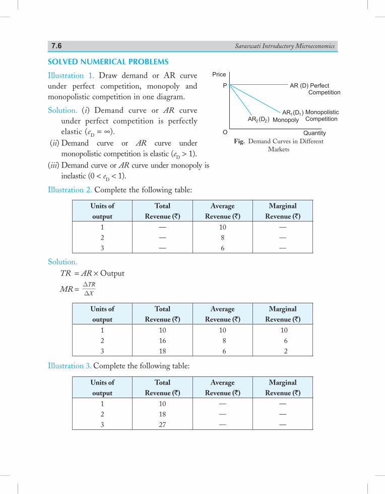
Saraswati Introductory Microeconomics7.6
Solved NUMeRiCAl PRobleMS
Illustration 1. Draw demand or AR curve under perfect competition, monopoly and monopolistic competition in one diagram.
Solution. (i) Demand curve or AR curve under perfect competition is perfectly elastic (eD = ∞).
(ii) Demand curve or AR curve under monopolistic competition is elastic (eD > 1).
(iii) Demand curve or AR curve under monopoly is inelastic (0 < eD < 1).
Illustration 2. Complete the following table:
Units ofoutput
Total Revenue (`)
AverageRevenue (`)
MarginalRevenue (`)
123
———
1086
———
Solution. TR = AR × Output
MR = DDTRX
Units ofoutput
Total Revenue (`)
AverageRevenue (`)
MarginalRevenue (`)
123
101618
1086
1062
Illustration 3. Complete the following table:
Units ofoutput
Total Revenue (`)
AverageRevenue (`)
MarginalRevenue (`)
123
101827
———
———
Fig. Demand Curves in Different Markets
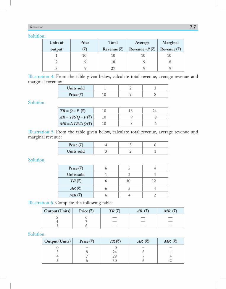
Revenue 7.7
Solution.Units of
output
Price
(`)
Total
Revenue (`)
Average
Revenue =P (`)
Marginal
Revenue (`)
1
2
3
10
9
9
10
18
27
10
9
9
10
8
9
Illustration 4. From the table given below, calculate total revenue, average revenue and marginal revenue:
Units sold 1 2 3
Price (`) 10 9 8
Solution.
TR = Q × P (`) 10 18 24
AR = TR/Q = P (`) 10 9 8
MR = �TR/�Q (`) 10 8 6
Illustration 5. From the table given below, calculate total revenue, average revenue and marginal revenue:
Price (`) 4 5 6
Units sold 3 2 1
Solution.
Price (`) 6 5 4
Units sold 1 2 3
TR (`) 6 10 12
AR (`) 6 5 4
MR (`) 6 4 2
Illustration 6. Complete the following table:
Output (Units) Price (`) TR (`) AR (`) MR (`)
543
678
———
———
———
Solution.Output (Units) Price (`) TR (`) AR (`) MR (`)
0345
–876
0242830
–876
––42

Saraswati Introductory Microeconomics7.8
Illustration 7. A perfectly competitive firm faces market price equal to ` 15.(a) Derive its total revenue schedule for the range of output from 0 to 10 units.(b) Suppose the market price increases to ̀ 17. Will the new TR curve be flatter or steeper?Solution.(a)
Output (Q) Price (`) TR = P × Q
0123
15151515
0153045
456789
10
15151515151515
607590
105120135150
(b) When price rises to ` 17, the new TR values will be: Output (Q1) Price (P1) TR1 = P1 × Q1
0123456789
10
1717171717171717171717
01734516885
102119136153170
The new TR curve (TR1) will be steeper.
Illustration 8. Complete the following table when each unit of a commodity can be sold at ` 5.
Quantity Sold(units)
TR(`)
MR(`)
AR(`)
1234567
———————
———————
———————
180160140120100
80604020O 1 2 3 4 5 6 7 8 9 10
Output
TRP
1 with= 17
TRP
with= 15T
R
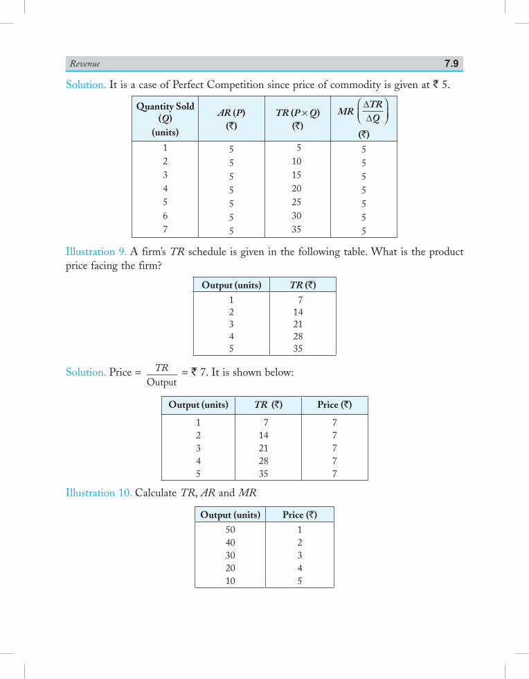
Revenue 7.9
Solution. It is a case of Perfect Competition since price of commodity is given at ` 5.
Quantity Sold (Q)
(units)
AR (P)(`)
TR (P × Q)(`)
MR ∆∆TRQ
(`)1234567
5555555
5101520253035
5555555
Illustration 9. A firm’s TR schedule is given in the following table. What is the product price facing the firm?
Output (units) TR (`)
12345
714212835
Solution. Price = TROutput
= ` 7. It is shown below:
Output (units) TR (`) Price (`)
12345
714212835
77777
Illustration 10. Calculate TR, AR and MR
Output (units) Price (`)
5040302010
12345
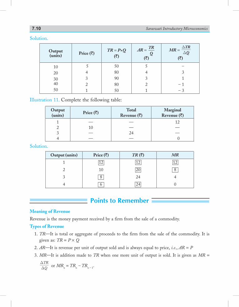
Saraswati Introductory Microeconomics7.10
Solution.
Output(units) Price (`)
TR = P×Q(`)
AR = TRQ
(`)
MR = DDTRQ
(`)
1020304050
54321
5080908050
54321
–31
– 1– 3
Illustration 11. Complete the following table:
Output (units)
Price (`)Total
Revenue (`)Marginal
Revenue (`)
1234
—10——
——24—
12——0
Solution.
Output (units) Price (`) TR (`) MR
1
2
3
4
12
10
8
6
12
20
24
24
12
8
4
0
Points to RememberMeaning of Revenue
Revenue is the money payment received by a firm from the sale of a commodity.
Types of Revenue
1. TR—It is total or aggregate of proceeds to the firm from the sale of the commodity. It is given as: TR = P × Q
2. AR—It is revenue per unit of output sold and is always equal to price, i.e., AR = P
3. MR—It is addition made to TR when one more unit of output is sold. It is given as MR = DD
TRQ or MRn = TRn – TRn – 1.
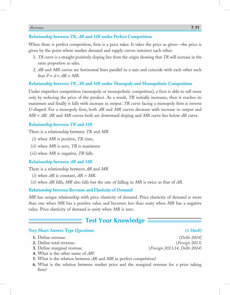
Revenue 7.11
Relationship between TR, AR and MR under Perfect Competition
When there is perfect competition, firm is a price taker. It takes the price as given—the price is given by the point where market demand and supply curves intersect each other.
1. TR curve is a straight positively sloping line from the origin showing that TR will in crease in the same proportion as sales.
2. AR and MR curves are horizontal lines parallel to x-axis and coincide with each other such that P = d = AR = MR.
Relationship between TR, AR and MR under Monopoly and Monopolistic Competition
Under imperfect competition (monopoly or monopolistic competiton), a firm is able to sell more only by reducing the price of the product. As a result, TR initially increases, then it reaches its maximum and finally it falls with increase in output. TR curve facing a monopoly firm is in verse U-shaped. For a monopoly firm, both AR and MR curves decrease with increase in output and MR < AR. AR and MR curves both are downward sloping and MR curve lies below AR curve.
Relationship between TR and MR
There is a relationship between TR and MR
(i) when MR is positive, TR rises,
(ii) when MR is zero, TR is maximum
(iii) when MR is negative, TR falls.
Relationship between AR and MR
There is a relationship between AR and MR (i) when AR is constant, AR = MR. (ii) when AR falls, MR also falls but the rate of falling in MR is twice as that of AR.
Relationship between Revenue and Elasticity of Demand
MR has unique relationship with price elasticity of demand. Price elasticity of demand is more than one when MR has a positive value and becomes less than unity when MR has a negative value. Price elasticity of demand is unity when MR is zero.
Test Your KnowledgeVery Short Answer Type Questions (1 Mark)
1. Define revenue. (Delhi 2014) 2. Define total revenue. (Foreign 2013) 3. Define marginal revenue. (Foreign 2013,14, Delhi 2014) 4. What is the other name of AR? 5. What is the relation between AR and MR in perfect competition? 6. What is the relation between market price and the marginal revenue for a price taking
firm?
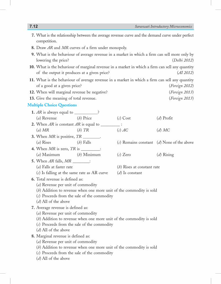
Saraswati Introductory Microeconomics7.12
7. What is the relationship between the average revenue curve and the demand curve under perfect competition.
8. Draw AR and MR curves of a firm under monopoly.
9. What is the behaviour of average revenue in a market in which a firm can sell more only by lowering the price? (Delhi 2012)
10. What is the behaviour of marginal revenue in a market in which a firm can sell any quantity of the output it produces at a given price? (AI 2012)
11. What is the behaviour of average revenue in a market in which a firm can sell any quantity of a good at a given price? (Foreign 2012)
12. When will marginal revenue be negative? (Foreign 2013) 13. Give the meaning of total revenue. (Foreign 2013)
Multiple Choice Questions
1. AR is always equal to ___________? (a) Revenue (b) Price (c) Cost (d) Profit 2. When AR is constant AR is equal to _________ : (a) MR (b) TR (c) AC (d) MC
3. When MR is positive, TR ________. (a) Rises (b) Falls (c) Remains constant (d) None of the above
4. When MR is zero, TR is _________: (a) Maximum (b) Minimum (c) Zero (d) Rising
5. When AR falls, MR ________: (a) Falls at faster rate (b) Rises at constant rate (c) Is falling at the same rate as AR curve (d) Is constant
6. Total revenue is defined as: (a) Revenue per unit of commodity (b) Addition to revenue when one more unit of the commodity is sold (c) Proceeds from the sale of the commodity (d) All of the above 7. Average revenue is defined as: (a) Revenue per unit of commodity (b) Addition to revenue when one more unit of the commodity is sold (c) Proceeds from the sale of the commodity (d) All of the above 8. Marginal revenue is defined as: (a) Revenue per unit of commodity (b) Addition to revenue when one more unit of the commodity is sold (c) Proceeds from the sale of the commodity (d) All of the above
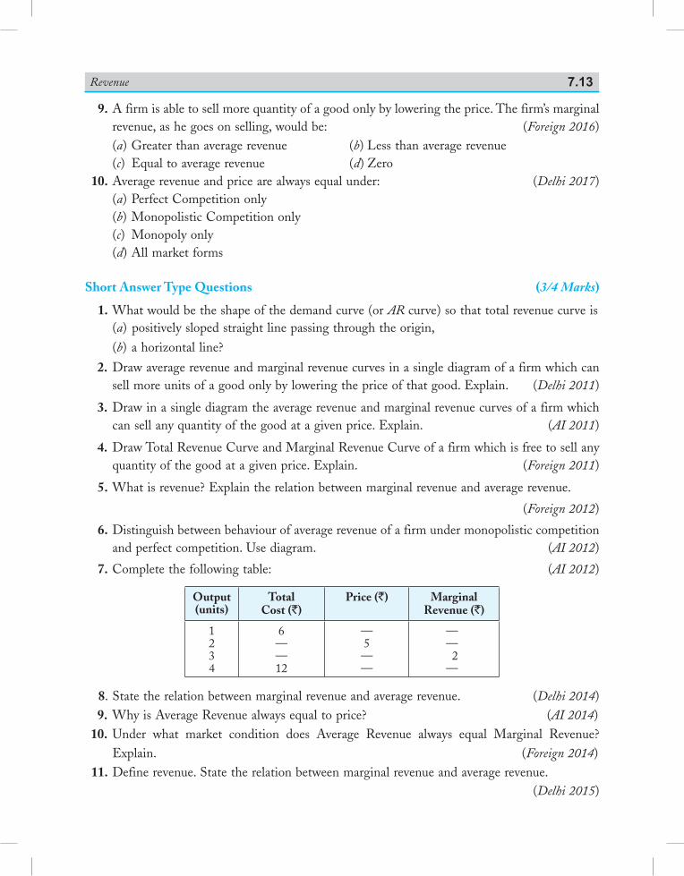
Revenue 7.13
9. A firm is able to sell more quantity of a good only by lowering the price. The firm’s marginal revenue, as he goes on selling, would be: (Foreign 2016)
(a) Greater than average revenue (b) Less than average revenue (c) Equal to average revenue (d) Zero 10. Average revenue and price are always equal under: (Delhi 2017) (a) Perfect Competition only (b) Monopolistic Competition only (c) Monopoly only (d) All market forms
Short Answer Type Questions (3/4 Marks)
1. What would be the shape of the demand curve (or AR curve) so that total revenue curve is(a) positively sloped straight line passing through the origin,(b) a horizontal line?
2. Draw average revenue and marginal revenue curves in a single diagram of a firm which can sell more units of a good only by lowering the price of that good. Explain. (Delhi 2011)
3. Draw in a single diagram the average revenue and marginal revenue curves of a firm which can sell any quantity of the good at a given price. Explain. (AI 2011)
4. Draw Total Revenue Curve and Marginal Revenue Curve of a firm which is free to sell any quantity of the good at a given price. Explain. (Foreign 2011)
5. What is revenue? Explain the relation between marginal revenue and average revenue.
(Foreign 2012)
6. Distinguish between behaviour of average revenue of a firm under monopolistic competition and perfect competition. Use diagram. (AI 2012)
7. Complete the following table: (AI 2012)
Output (units)
TotalCost (`)
Price (`) MarginalRevenue (`)
1234
6——12
—5——
——2
—
8. State the relation between marginal revenue and average revenue. (Delhi 2014) 9. Why is Average Revenue always equal to price? (AI 2014) 10. Under what market condition does Average Revenue always equal Marginal Revenue?
Explain. (Foreign 2014) 11. Define revenue. State the relation between marginal revenue and average revenue. (Delhi 2015)
Saraswati Introductory Microeconomics7.14
Long Answer Type Questions (6 Marks)
1. Prepare a schedule based on imaginary data about TR, AR and MR assuming that the price is same at all levels of output.
2. Prepare an imaginary TR, AR and MR schedule in a market situation in which the firm is able to sell more only by reducing the price of the product.
3. Explain the relationship between: (Foreign 2010) (i) Marginal revenue and Total revenue (ii) Marginal revenue and Average revenue
AnswersMultiple Choice Questions
1. (b) 2. (a) 3. (a) 4. (a) 5. (a) 6. (c) 7. (a) 8. (b)
9. (b) 10. (a)
8.1 Meaning of producer’s equilibriuM
A producer is said to be in equilibrium when he produces that level of output at which his profits are maximum. Profit equals total revenue minus total cost. Producer’s equilibrium is also known as profit maximisation situation.
8.2 producer’s equilibriuM (i.e. profit MaxiMisation conditions of the producer) through Mr and Mc approach
According to MR and MC approach, a producer or a firm is said to be in equilibrium when it satisfies the following two conditions of equilibrium.The equilibrium conditions are:
MR = MC …(1)
Slope of MR < Slope of MC …(2)
The second condition means that MC is greater than MR after the output level where MR = MC. In other words, MC curve must be rising at the point of equilibrium or MC curve must cut MR curve from below.
Explanation of Equilibrium ConditionsFirst condition: MC = MR
MR is the additional revenue from selling one more unit of output of a good and MC is the additional cost of producing one more unit of output of the good. In other words, if the gain (i.e., MR) is greater than the cost (i.e., MC) then it is profitable to produce more units of that good.Now suppose a producer or a firm starts production when it finds that MR > MC. It will continue to produce as long as MR becomes equal to MC. At that level of output of the good 1st condition i.e., MC = MR is satisfied.
Chapter Scheme
Producer’s Equilibrium 8
8.4 Monopoly or Monopolistic Competition Solved Numerical Problems Points to Remember Test Your Knowledge Answers to MCQs
8.1 Meaning of Producer’s Equilibrium8.2Producer’sEquilibrium(i.e.Profit
Maximisation Conditions of the Producer)Through MR and MC Approach
8.3 Perfect Competition
Saraswati Introductory Microeconomics8.2
Second condition: MC > MR after the MC = MR level of output
Whether a producer is in equilibrium or not, it will depend upon the condition that—beyond that level of output, MC must be more than MR and before that level of output, MC must be less than MR.
If beyond that level of output, a producer found that MC < MR by producing any more unit of output, it means that it is profitable to produce an extra unit. When MC > MR beyond MC = MR level of output, it means that it is unprofitable to produce an extra unit. It starts reducing the level of output till MR = MC.
Table 8.1 Tabular Presentation of Producer’s Equilibrium
Units of Output
Produced and Sold
Price(`)
TR(`)
TC(`)
MC(`)
MR(`)
EquilibriumCondition
1 20 20 20 20 20 MC = MR
2 20 40 36 16 20
3 20 60 48 12 20
4 20 80 56 18 20 MC < MR
5 20 100 68 12 20
6 20 120 84 16 20
7 20 140 104 20 20 Equilibrium
8 20 160 128 24 20 MC > MR
At 7 units of output the producer is in equilibrium because it satisfies both MR and MC conditions. That is, at 7 units of output (i) MR = MC = ` 20, and (ii) after this level of output, MC (` 24) becomes greater than MR (` 20).
8.3 perfect coMpetition
Graphical presentation of profit maximization conditions under perfect competition.
Consider Fig. 8.1.
1. P > MC. At output X2, price is FX2 and MC is NX2. So, P > MC. X2 is not the profit maximising level of output because firm’s profit is higher when firm expands its output level to OX3 level.
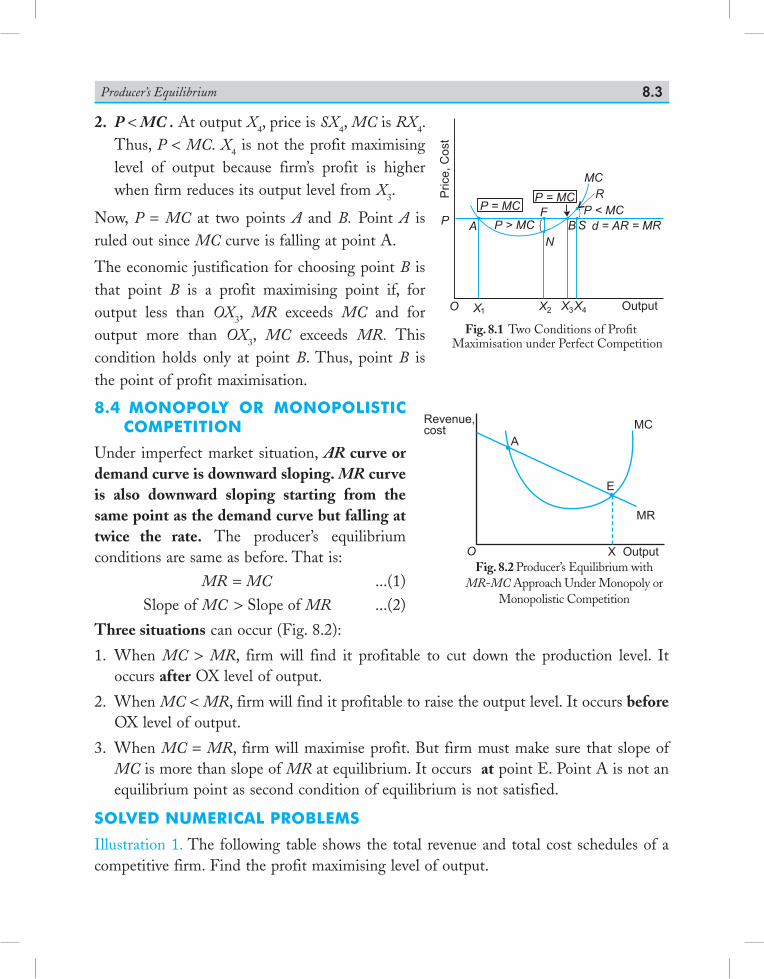
Producer’s Equilibrium 8.3
2. P < MC . At output X4, price is SX4, MC is RX4. Thus, P < MC. X4 is not the profit maximising level of output because firm’s profit is higher when firm reduces its output level from X3.
Now, P = MC at two points A and B. Point A is ruled out since MC curve is falling at point A.
The economic justification for choosing point B is that point B is a profit maximising point if, for output less than OX3, MR exceeds MC and for output more than OX3, MC exceeds MR. This condition holds only at point B. Thus, point B is the point of profit maximisation.
8.4 Monopoly or Monopolistic coMpetition
Under imperfect market situation, AR curve or demand curve is downward sloping. MR curve is also downward sloping starting from the same point as the demand curve but falling at twice the rate. The producer’s equilibrium conditions are same as before. That is: MR = MC ...(1) Slope of MC >Slope of MR ...(2)
Three situations can occur (Fig. 8.2):
1. When MC > MR, firm will find it profitable to cut down the production level. It occurs after OX level of output.
2. When MC < MR, firm will find it profitable to raise the output level. It occurs before OX level of output.
3. When MC = MR, firm will maximise profit. But firm must make sure that slope of MC is more than slope of MR at equilibrium. It occurs at point E. Point A is not an equilibrium point as second condition of equilibrium is not satisfied.
solved nuMerical probleMs
Illustration 1. The following table shows the total revenue and total cost schedules of a competitive firm. Find the profit maximising level of output.
1 2 3 4
Fig. 8.1 Two Conditions of Profit Maximisation under Perfect Competition
Revenue,cost
O
A
E
X Output
MC
MR
Fig. 8.2 Producer’s Equilibrium with MR-MC Approach Under Monopoly or
Monopolistic Competition
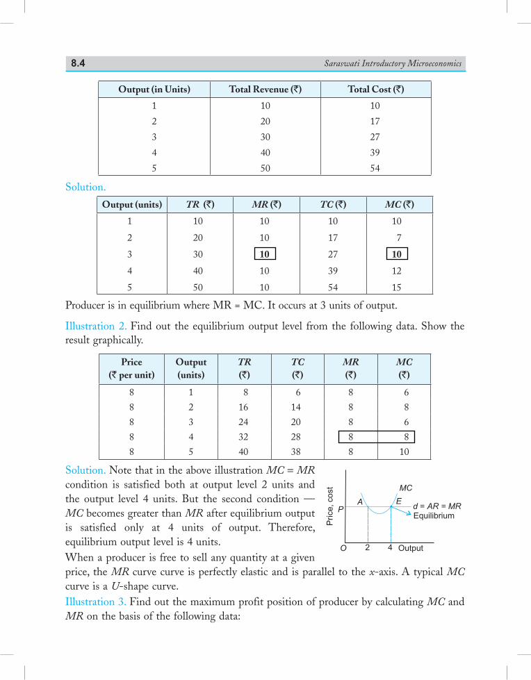
Saraswati Introductory Microeconomics8.4
Output (in Units) Total Revenue (`) Total Cost (`)
1
2
3
4
5
10
20
30
40
50
10
17
27
39
54
Solution.
Output (units) TR (`) MR (`) TC (`) MC (`)
1
2
3
4
5
10
20
30
40
50
10
10
10
10
10
10
17
27
39
54
10
7
10
12
15
Producer is in equilibrium where MR = MC. It occurs at 3 units of output.
Illustration 2. Find out the equilibrium output level from the following data. Show the result graphically.
Price (` per unit)
Output (units)
TR (`)
TC (`)
MR (`)
MC (`)
8 1 8 6 8 6
8 2 16 14 8 8
8 3 24 20 8 6
8 4 32 28 8 8
8 5 40 38 8 10
Solution. Note that in the above illustration MC = MR condition is satisfied both at output level 2 units and the output level 4 units. But the second condition — MC becomes greater than MR after equilibrium output is satisfied only at 4 units of output. Therefore, equilibrium output level is 4 units.When a producer is free to sell any quantity at a given price, the MR curve curve is perfectly elastic and is parallel to the x-axis. A typical MC curve is a U-shape curve.Illustration 3. Find out the maximum profit position of producer by calculating MC and MR on the basis of the following data:
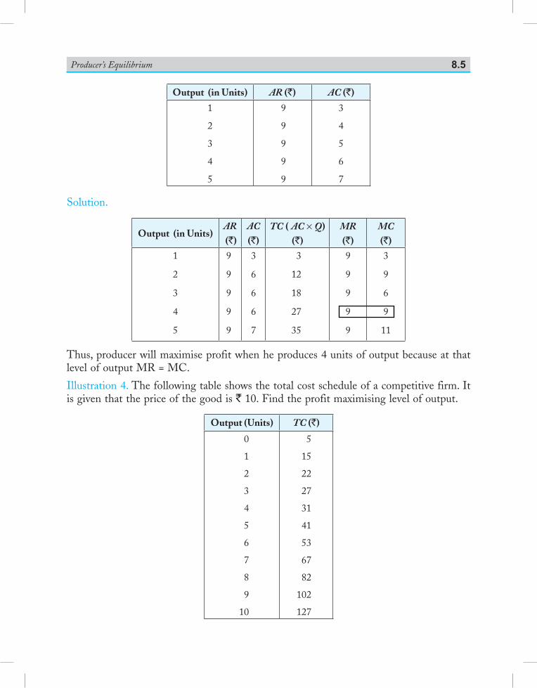
Producer’s Equilibrium 8.5
Output (in Units) AR (`) AC (`)
1
2
3
4
5
9
9
9
9
9
3
4
5
6
7
Solution.
Output (in Units)AR (`)
AC(`)
TC ( AC × Q)(`)
MR(`)
MC(`)
1
2
3
4
5
9
9
9
9
9
3
6
6
6
7
3
12
18
27
35
9
9
9
9
9
3
9
6
9
11
Thus, producer will maximise profit when he produces 4 units of output because at that level of output MR = MC.
Illustration 4. The following table shows the total cost schedule of a competitive firm. It is given that the price of the good is ` 10. Find the profit maximising level of output.
Output (Units) TC (`)
0
1
2
3
4
5
6
7
8
9
10
5
15
22
27
31
41
53
67
82
102
127
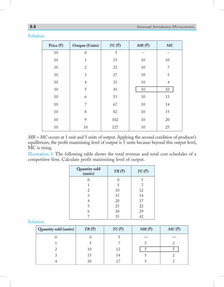
Saraswati Introductory Microeconomics8.6
Solution.
Price (`) Output (Units) TC (`) MR (`) MC
10 0 5 – –
10 1 15 10 10
10 2 22 10 7
10 3 27 10 5
10 4 31 10 4
10 5 41 10 10
10 6 53 10 13
10 7 67 10 14
10 8 82 10 15
10 9 102 10 20
10 10 127 10 25
MR = MC occurs at 1 unit and 5 units of output. Applying the second condition of producer’s equilibrium, the profit maximising level of output is 5 units because beyond this output level, MC is rising.Illustration 5. The following table shows the total revenue and total cost schedules of a competitive firm. Calculate profit maximising level of output.
Quantity sold (units) TR (`) TC (`)
01234567
05
101520253035
57
121417222942
Solution.
Quantity sold (units) TR (`) TC (`) MR (`) MC (`)
01234
05
101520
57
121417
—5555
—2523
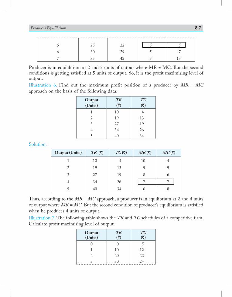
Producer’s Equilibrium 8.7
5
6
7
25
30
35
22
29
42
5
5
5
5
7
13
Producer is in equilibrium at 2 and 5 units of output where MR = MC. But the second conditions is getting satisfied at 5 units of output. So, it is the profit maximising level of output.Illustration 6. Find out the maximum profit position of a producer by MR – MC approach on the basis of the following data:
Output(Units)
TR(`)
TC(`)
12345
1019273440
413192634
Solution.
Output (Units) TR (`) TC (`) MR (`) MC (`)
1
2
3
4
5
10
19
27
34
40
4
13
19
26
34
10
9
8
7
6
4
9
6
7
8
Thus, according to the MR – MC approach, a producer is in equilibrium at 2 and 4 units of output where MR = MC. But the second condition of producer’s equilibrium is satisfied when he produces 4 units of output.Illustration 7. The following table shows the TR and TC schedules of a competitive firm. Calculate profit maximising level of output.
Output(Units)
TR(`)
TC(`)
0123
0102030
5122224
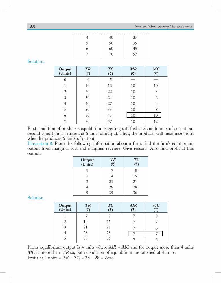
Saraswati Introductory Microeconomics8.8
4567
40506070
27354557
Solution.
Output(Units)
TR (`)
TC(`)
MR(`)
MC(`)
01234567
010203040506070
512222427354557
—10
101010101010
—105238
1012
First condition of producers equilibrium is getting satisfied at 2 and 6 units of output but second condition is satisfied at 6 units of output. Thus, the producer will maximise profit when he produces 6 units of output. Illustration 8. From the following information about a firm, find the firm’s equilibrium output from marginal cost and marginal revenue. Give reasons. Also find profit at this output.
Output(Units)
TR(`)
TC(`)
12345
714212835
815212836
Solution.
Output(Units)
TR (`)
TC(`)
MR(`)
MC(`)
12345
714212835
815212836
77
777
87678
Firms equilibrium output is 4 units where MR = MC and for output more than 4 units MC is more than MR so, both condition of equilibrium are satisfied at 4 units. Profit at 4 units = TR – TC = 28 – 28 = Zero
Producer’s Equilibrium 8.9
Points to Remember
Meaning of Producer’s Equilibrium
1. A producer is an economic agent who produces goods and services for sale.
2. The objective of a producer is always to maximise his profits.
3. A producer is said to be in equilibrium when he produces the level of output at which his profits
are maximum.
Conditions of Producer’s Equilibrium
Under MR – MC approach, a producer is in equilibrium, (i.e., maximises profits) at that level
of output where (i) MR = MC and (ii) MC is rising.
Conditions of Producer’s Equilibrium under Perfect Competition and Monopoly or Monopolistic
Competition
1. In a perfectly competitive market, the marginal revenue and average revenue of a producer
coincide and is equal to market price, i.e., AR = MR = P. A competitive producer’s equilibrium
is established at that level of output where,
(i) P = MC, (ii) MC is rising and (iii) P > AVC in short-run and P > AC in the long-run. In
a situation of equilibrium, a producer may be earning maximum profit, break-even or
shut-down.
A competitive producer always choose that level of output which lies on the rising portion
of the MC curve. He will never produce on the decreasing portion of the MC curve. MC
curve gives the supply curve of the firm.
2. Under monopoly or monopolistic competition, conditions of producer’s equilibrium are
MR = MC and slope of MC > slope of MR.
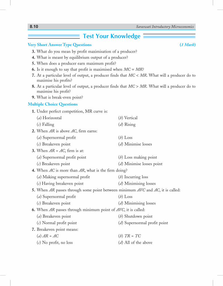
Saraswati Introductory Microeconomics8.10
Test Your KnowledgeVery Short Answer Type Questions (1 Mark)
3. What do you mean by profit maximisation of a producer? 4. What is meant by equilibrium output of a producer? 5. When does a producer earn maximum profit? 6. Is it enough to say that profit is maximised when MC = MR? 7. At a particular level of output, a producer finds that MC < MR. What will a producer do to
maximise his profits? 8. At a particular level of output, a producer finds that MC > MR. What will a producer do to
maximise his profit? 9. What is break-even point?
Multiple Choice Questions
1. Under perfect competition, MR curve is:
(a ) Horizontal (b) Vertical
(c) Falling (d) Rising
2. When AR is above AC, firm earns:
(a) Supernormal profit (b) Loss
(c) Breakeven point (d) Minimise losses
3. When AR = AC, firm is at:
(a) Supernormal profit point (b) Loss making point
(c) Breakeven point (d) Minimise losses point
4. When AC is more than AR, what is the firm doing?
(a) Making supernormal profit (b) Incurring loss
(c) Having breakeven point (d) Minimising losses
5. When AR passes through some point between minimum AVC and AC, it is called:
(a) Supernormal profit (b) Loss
(c) Breakeven point (d) Minimising losses
6. When AR passes through minimum point of AVC, it is called:
(a) Breakeven point (b) Shutdown point
(c) Normal profit point (d) Supernormal profit point
7. Breakeven point means:
(a) AR = AC (b) TR = TC
(c) No profit, no loss (d) All of the above
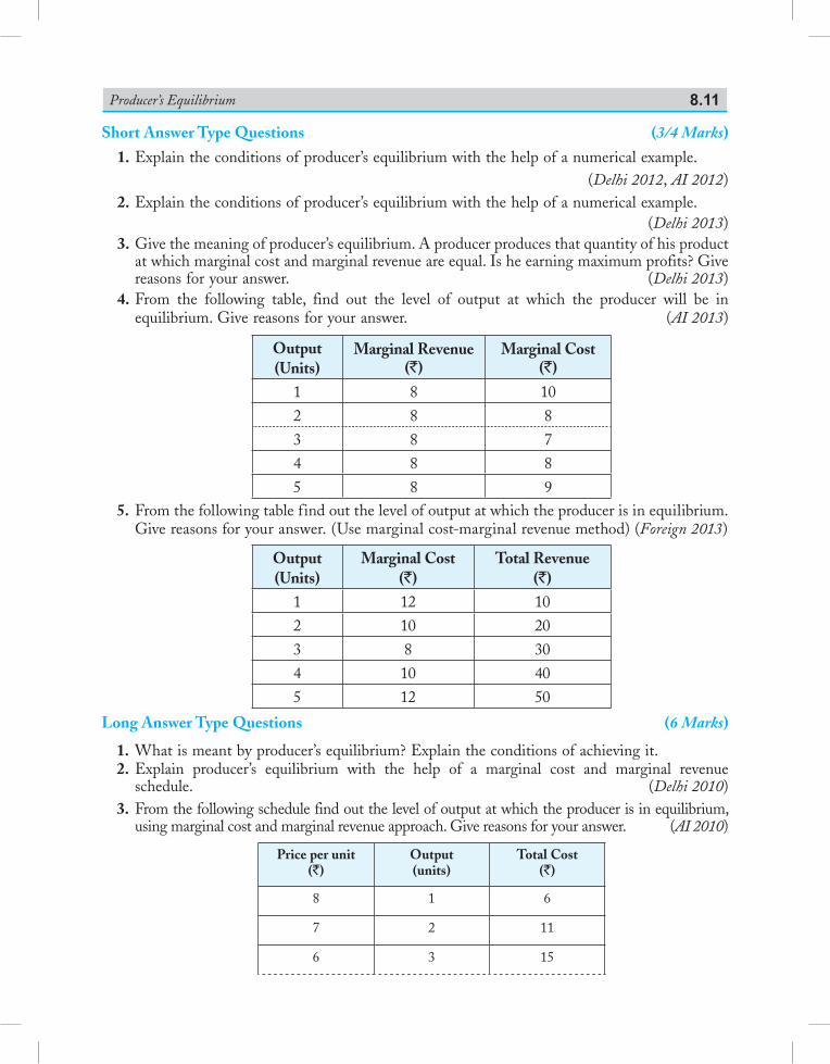
Producer’s Equilibrium 8.11
Short Answer Type Questions (3/4 Marks)
1. Explain the conditions of producer’s equilibrium with the help of a numerical example.(Delhi 2012, AI 2012)
2. Explain the conditions of producer’s equilibrium with the help of a numerical example. (Delhi 2013) 3. Give the meaning of producer’s equilibrium. A producer produces that quantity of his product
at which marginal cost and marginal revenue are equal. Is he earning maximum profits? Give reasons for your answer. (Delhi 2013)
4. From the following table, find out the level of output at which the producer will be in equilibrium. Give reasons for your answer. (AI 2013)
Output(Units)
Marginal Revenue(`)
Marginal Cost(`)
1 8 102 8 83 8 74 8 85 8 9
5. From the following table find out the level of output at which the producer is in equilibrium. Give reasons for your answer. (Use marginal cost-marginal revenue method) (Foreign 2013)
Output(Units)
Marginal Cost(`)
Total Revenue(`)
1 12 102 10 203 8 304 10 405 12 50
Long Answer Type Questions (6 Marks)
1. What is meant by producer’s equilibrium? Explain the conditions of achieving it. 2. Explain producer’s equilibrium with the help of a marginal cost and marginal revenue
schedule. (Delhi 2010) 3. From the following schedule find out the level of output at which the producer is in equilibrium,
using marginal cost and marginal revenue approach. Give reasons for your answer. (AI 2010)
Price per unit(`)
Output(units)
Total Cost (`)
8 1 6
7 2 11
6 3 15
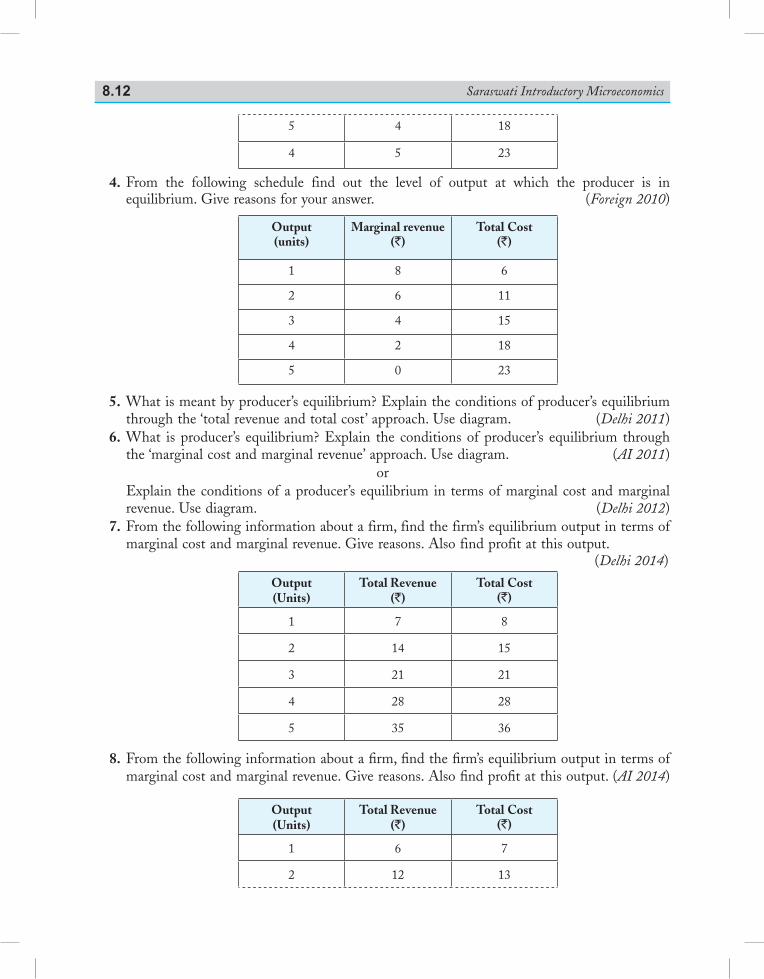
Saraswati Introductory Microeconomics8.12
5 4 18
4 5 23
4. From the following schedule find out the level of output at which the producer is in equilibrium. Give reasons for your answer. (Foreign 2010)
Output(units)
Marginal revenue(`)
Total Cost (`)
1 8 6
2 6 11
3 4 15
4 2 18
5 0 23
5. What is meant by producer’s equilibrium? Explain the conditions of producer’s equilibrium through the ‘total revenue and total cost’ approach. Use diagram. (Delhi 2011)
6. What is producer’s equilibrium? Explain the conditions of producer’s equilibrium through the ‘marginal cost and marginal revenue’ approach. Use diagram. (AI 2011)
or Explain the conditions of a producer’s equilibrium in terms of marginal cost and marginal
revenue. Use diagram. (Delhi 2012) 7. From the following information about a firm, find the firm’s equilibrium output in terms of
marginal cost and marginal revenue. Give reasons. Also find profit at this output. (Delhi 2014)
Output(Units)
Total Revenue(`)
Total Cost (`)
1 7 8
2 14 15
3 21 21
4 28 28
5 35 36
8. From the following information about a firm, find the firm’s equilibrium output in terms of marginal cost and marginal revenue. Give reasons. Also find profit at this output. (AI 2014)
Output(Units)
Total Revenue(`)
Total Cost (`)
1 6 7
2 12 13
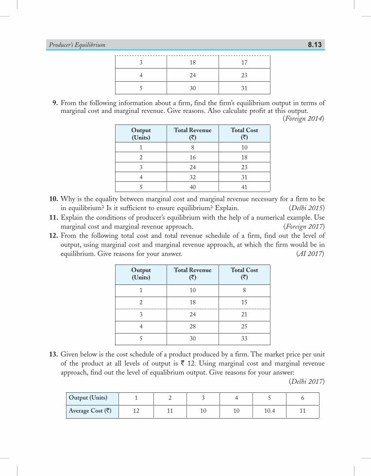
Producer’s Equilibrium 8.13
3 18 17
4 24 23
5 30 31
9. From the following information about a firm, find the firm’s equilibrium output in terms of marginal cost and marginal revenue. Give reasons. Also calculate profit at this output.
(Foreign 2014)
Output(Units)
Total Revenue(`)
Total Cost (`)
1 8 10
2 16 18
3 24 23
4 32 31
5 40 41
10. Why is the equality between marginal cost and marginal revenue necessary for a firm to be in equilibrium? Is it sufficient to ensure equilibrium? Explain. (Delhi 2015)
11. Explain the conditions of producer’s equilibrium with the help of a numerical example. Use marginal cost and marginal revenue approach. (Foreign 2017)
12. From the following total cost and total revenue schedule of a firm, find out the level of output, using marginal cost and marginal revenue approach, at which the firm would be in equilibrium. Give reasons for your answer. (AI 2017)
Output(Units)
Total Revenue(`)
Total Cost (`)
1 10 8
2 18 15
3 24 21
4 28 25
5 30 33
13. Given below is the cost schedule of a product produced by a firm. The market price per unit of the product at all levels of output is ` 12. Using marginal cost and marginal revenue approach, find out the level of equalibrium output. Give reasons for your answer:
(Delhi 2017)
Output (Units) 1 2 3 4 5 6
Average Cost (`) 12 11 10 10 10.4 11
Saraswati Introductory Microeconomics8.14
AnswersMultiple Choice Questions
1. (a) 2. (a) 3. (c) 4. (b) 5. (d) 6. (b) 7. (d)
9.1 ConCept of Supply
9.1.1 Meaning of SupplySupply of a commodity means quantity of the commodity which a firm is willing to sell at a given price during a particular time. Like demand, supply definition is complete when it has the following elements: (i) Quantity of a commodity that the producer is willing to offer for sale, (ii) Price of the commodity, and (iii) Time during which the quantity is offered for sale.Example. Firm A supplies 50 kg of wheat at price of ` 10 per kg in a month is a statement of supply.
9.1.2 Difference between Supply and StockStock of a commodity is the total quantity that is available in a market at a certain time.
Chapter Scheme9.1 Concept of Supply 9.1.1 Meaning of Supply 9.1.2 Difference between Supply and Stock9.2 Supply Function and its Slope9.3 Factors Affecting Supply of a
Commodity 9.3.1 Price of the Commodity 9.3.2 Price of Related Good (Z) 9.3.3 State of Technology 9.3.4 Prices of Inputs 9.3.5 Government Policy9.4 The Law of Supply 9.4.1 Meaning and Assumptions of the
Law of Supply 9.4.2 The Supply Schedule and the Supply
Curve 9.4.3 Reasons Behind Upward Sloping
Supply Curve9.5 From Individual Supply to Market
Supply 9.5.1 Construction of Individual and
Market Supply Schedule
9.5.2 Construction of Individual and Market Supply Curve
9.6 Change in Quantity Supplied vs. Change in Supply
9.6.1 Change in Quantity Supplied (Movement)
9.6.2 Change in Supply (Shift) 9.6.3 Difference between Movement and
Shift of the Supply Curve9.7 Elasticity of Supply 9.7.1DefinitionofElasticityofSupply 9.7.2DeterminantsofElasticityofSupply9.8 Different Types of Elasticity of Supply9.9 Measurement of Elasticity of Supply Percentage Method Solved Numerical Problems Points to Remember Test Your Knowledge Answers to MCQs
Supply and Elasticity of Supply 9
Saraswati Introductory Microeconomics9.2
Supply is that part of the stock which a seller is ready to sell at a certain price during a certain time. Thus, supply is that part of stock which is actually brought into the market.For example, a producer has produced 400 pencils. This is the stock of pencils with him. He may be willing to offer for sale 100 pencils at the rate of ` 10 per pencil, 120 pencils at ` 20 each; 150 pencils at ` 30 each and so on. In this case, stock is 400 pencils, but the supply of pencils is different at different prices.
9.2 Supply funCtion and itS SlopeSupply function is a functional relationship between quantity supplied of a commodity and factors affecting it. The supply function can be written as:
SX = f (PX, PZ, T, C, GP)where, SX = Supply of commodity X f = function of PX = Price of commodity X P = Price of related good, Z T = Technological changes C = Cost of production or price of inputs GP = Government policy or excise tax rate.
Slope of supply function is given as ∆∆PQ
. It measures the rate at which supply curve slopes
upwards. In other words, it measures the rate at which supply changes with respect to its price.
9.3 faCtorS affeCting Supply of a Commodity
9.3.1 Price of the CommodityAt a higher price, producer offers more quantity of the commodity for sale and at a lower price, less quantity of the commodity is offered for sale. There is a direct relationship between price and quantity supplied as shown by law of supply.
9.3.2 Price of Related Good (Z)Supply of a commodity depends upon the prices of its related goods, specially substitute goods. If the price of a commodity remains constant and the price of its substitute good Z increases, the producers would prefer to produce substitute good Z. As a result, the supply of commodity X will decrease and that of substitute good Z will increase. This will shift the supply curve of good X leftward. Thus, an increase in the price of substitute good will lead to decrease in supply curve of the other good and vice-versa.
9.3.3 State of TechnologyIf there is a change in the technique of production leading to a fall in the cost of produc-tion, supply of commodity will increase.
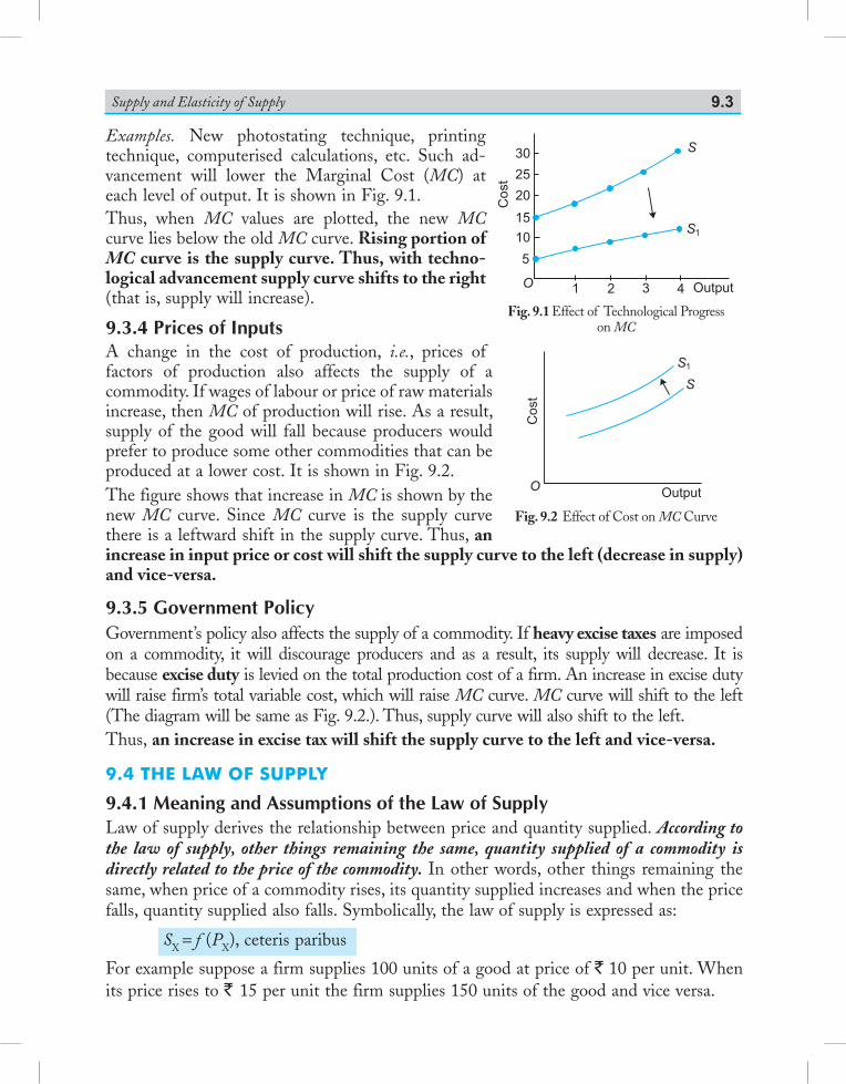
Supply and Elasticity of Supply 9.3
Examples. New photostating technique, printing technique, computerised calculations, etc. Such ad-vancement will lower the Marginal Cost (MC) at each level of output. It is shown in Fig. 9.1.Thus, when MC values are plotted, the new MC curve lies below the old MC curve. Rising portion of MC curve is the supply curve. Thus, with techno-logical advancement supply curve shifts to the right (that is, supply will increase).
9.3.4 Prices of InputsA change in the cost of production, i.e., prices of factors of production also affects the supply of a commodity. If wages of labour or price of raw materials increase, then MC of production will rise. As a result, supply of the good will fall because producers would prefer to produce some other commodities that can be produced at a lower cost. It is shown in Fig. 9.2.The figure shows that increase in MC is shown by the new MC curve. Since MC curve is the supply curve there is a leftward shift in the supply curve. Thus, an increase in input price or cost will shift the supply curve to the left (decrease in supply) and vice-versa.
9.3.5 Government PolicyGovernment’s policy also affects the supply of a commodity. If heavy excise taxes are imposed on a commodity, it will discourage producers and as a result, its supply will decrease. It is because excise duty is levied on the total production cost of a firm. An increase in excise duty will raise firm’s total variable cost, which will raise MC curve. MC curve will shift to the left (The diagram will be same as Fig. 9.2.). Thus, supply curve will also shift to the left.Thus, an increase in excise tax will shift the supply curve to the left and vice-versa.
9.4 the law of Supply
9.4.1 Meaning and Assumptions of the Law of SupplyLaw of supply derives the relationship between price and quantity supplied. According to the law of supply, other things remaining the same, quantity supplied of a commodity is directly related to the price of the commodity. In other words, other things remaining the same, when price of a commodity rises, its quantity supplied increases and when the price falls, quantity supplied also falls. Symbolically, the law of supply is expressed as:
SX = f (PX), ceteris paribus
For example suppose a firm supplies 100 units of a good at price of ` 10 per unit. When its price rises to ` 15 per unit the firm supplies 150 units of the good and vice versa.
Fig. 9.1 Effect of Technological Progress on MC
Fig. 9.2 Effect of Cost on MC Curve
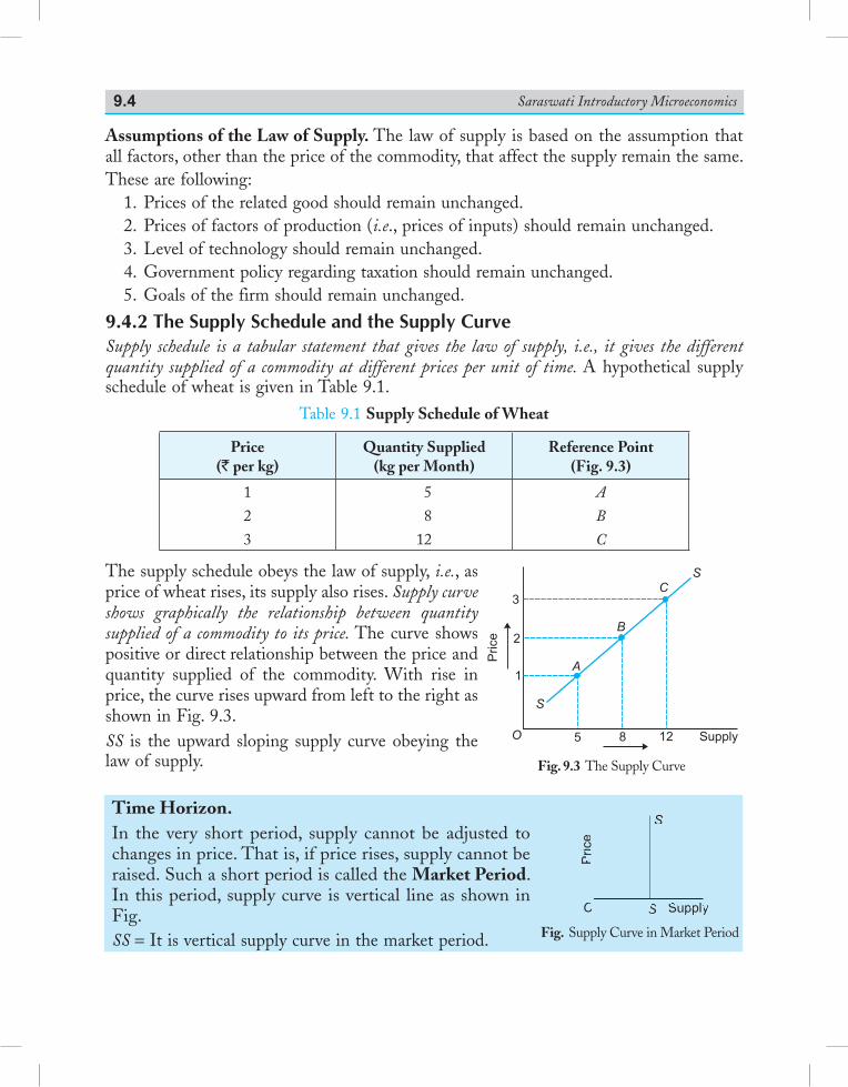
Saraswati Introductory Microeconomics9.4
Assumptions of the Law of Supply. The law of supply is based on the assumption that all factors, other than the price of the commodity, that affect the supply remain the same.These are following: 1. Prices of the related good should remain unchanged. 2. Prices of factors of production (i.e., prices of inputs) should remain unchanged. 3. Level of technology should remain unchanged. 4. Government policy regarding taxation should remain unchanged. 5. Goals of the firm should remain unchanged.
9.4.2 The Supply Schedule and the Supply CurveSupply schedule is a tabular statement that gives the law of supply, i.e., it gives the different quantity supplied of a commodity at different prices per unit of time. A hypothetical supply schedule of wheat is given in Table 9.1.
Table 9.1 Supply Schedule of Wheat
Price (` per kg)
Quantity Supplied (kg per Month)
Reference Point (Fig. 9.3)
1
2
3
5
8
12
A
B
C
The supply schedule obeys the law of supply, i.e., as price of wheat rises, its supply also rises. Supply curve shows graphically the relationship between quantity supplied of a commodity to its price. The curve shows positive or direct relationship between the price and quantity supplied of the commodity. With rise in price, the curve rises upward from left to the right as shown in Fig. 9.3.SS is the upward sloping supply curve obeying the law of supply.
Time Horizon.In the very short period, supply cannot be adjusted to changes in price. That is, if price rises, supply cannot be raised. Such a short period is called the Market Period. In this period, supply curve is vertical line as shown in Fig.SS = It is vertical supply curve in the market period.
A
B
C
S
S
O
3
2
1
5 8 12 Supply
Price
Fig. 9.3 The Supply Curve
Fig. Supply Curve in Market Period
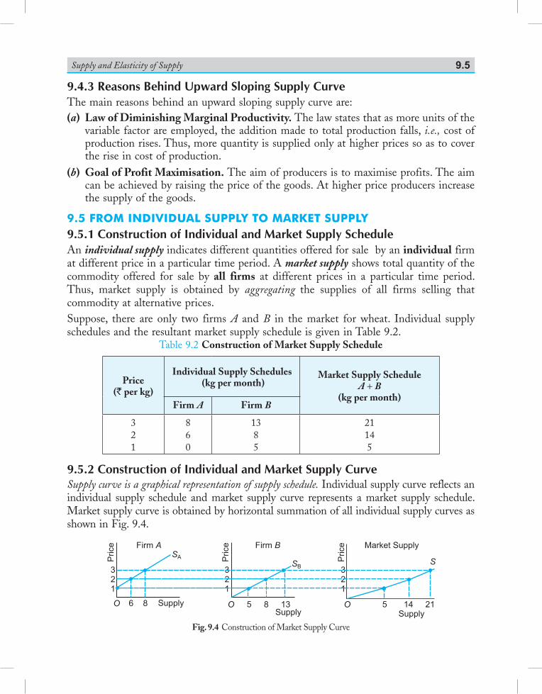
Supply and Elasticity of Supply 9.5
9.4.3 Reasons Behind Upward Sloping Supply CurveThe main reasons behind an upward sloping supply curve are:(a) Law of Diminishing Marginal Productivity. The law states that as more units of the
variable factor are employed, the addition made to total production falls, i.e., cost of production rises. Thus, more quantity is supplied only at higher prices so as to cover the rise in cost of production.
(b) Goal of Profit Maximisation. The aim of producers is to maximise profits. The aim can be achieved by raising the price of the goods. At higher price producers increase the supply of the goods.
9.5 from individual Supply to market Supply9.5.1 Construction of Individual and Market Supply ScheduleAn individual supply indicates different quantities offered for sale by an individual firm at different price in a particular time period. A market supply shows total quantity of the commodity offered for sale by all firms at different prices in a particular time period. Thus, market supply is obtained by aggregating the supplies of all firms selling that commodity at alternative prices.Suppose, there are only two firms A and B in the market for wheat. Individual supply schedules and the resultant market supply schedule is given in Table 9.2.
Table 9.2 Construction of Market Supply Schedule
Price (` per kg)
Individual Supply Schedules (kg per month)
Market Supply Schedule A + B
(kg per month)Firm A Firm B
321
860
1385
21145
9.5.2 Construction of Individual and Market Supply CurveSupply curve is a graphical representation of supply schedule. Individual supply curve reflects an individual supply schedule and market supply curve represents a market supply schedule. Market supply curve is obtained by horizontal summation of all individual supply curves as shown in Fig. 9.4.
Fig. 9.4 Construction of Market Supply Curve
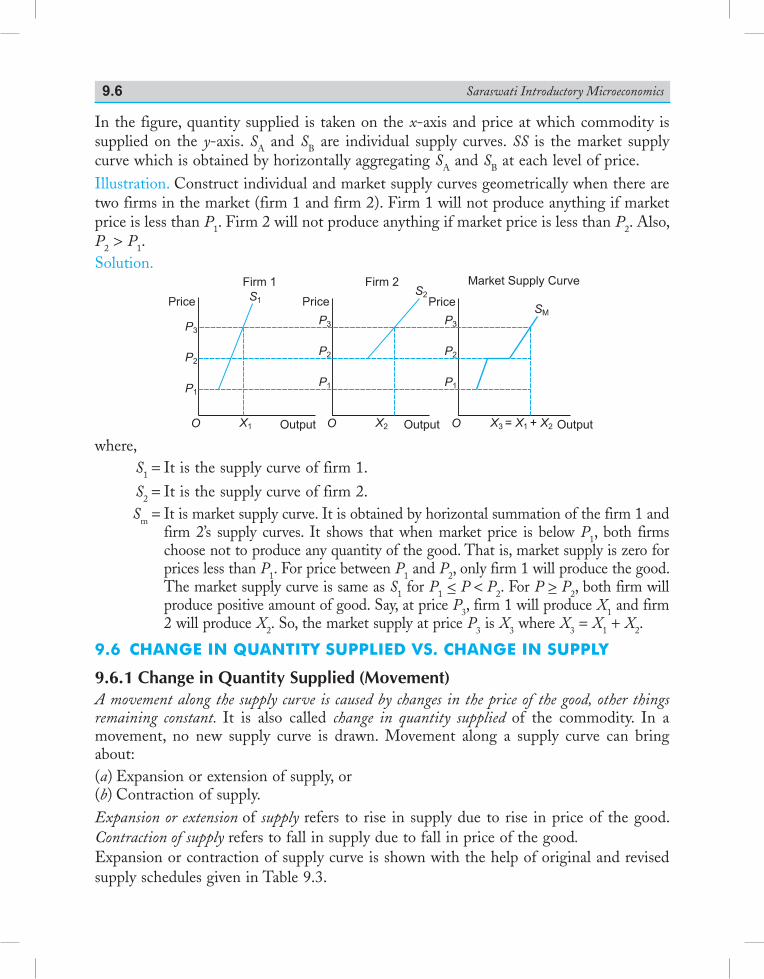
Saraswati Introductory Microeconomics9.6
In the figure, quantity supplied is taken on the x-axis and price at which commodity is supplied on the y-axis. SA and SB are individual supply curves. SS is the market supply curve which is obtained by horizontally aggregating SA and SB at each level of price.Illustration. Construct individual and market supply curves geometrically when there are two firms in the market (firm 1 and firm 2). Firm 1 will not produce anything if market price is less than P1. Firm 2 will not produce anything if market price is less than P2. Also, P2 > P1.Solution.
where, S1 = It is the supply curve of firm 1. S2 = It is the supply curve of firm 2. Sm = It is market supply curve. It is obtained by horizontal summation of the firm 1 and
firm 2’s supply curves. It shows that when market price is below P1, both firms choose not to produce any quantity of the good. That is, market supply is zero for prices less than P1. For price between P1 and P2, only firm 1 will produce the good. The market supply curve is same as S1 for P1 < P < P2. For P > P2, both firm will produce positive amount of good. Say, at price P3, firm 1 will produce X1 and firm 2 will produce X2. So, the market supply at price P3 is X3 where X3 = X1 + X2.
9.6 Change in Quantity Supplied vS. Change in Supply
9.6.1 Change in Quantity Supplied (Movement)A movement along the supply curve is caused by changes in the price of the good, other things remaining constant. It is also called change in quantity supplied of the commodity. In a movement, no new supply curve is drawn. Movement along a supply curve can bring about:(a) Expansion or extension of supply, or(b) Contraction of supply.Expansion or extension of supply refers to rise in supply due to rise in price of the good. Contraction of supply refers to fall in supply due to fall in price of the good.Expansion or contraction of supply curve is shown with the help of original and revised supply schedules given in Table 9.3.
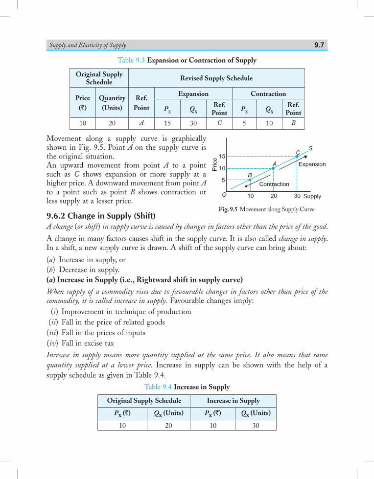
Supply and Elasticity of Supply 9.7
Table 9.3 Expansion or Contraction of Supply
Original Supply Schedule Revised Supply Schedule
Price(`)
Quantity(Units)
Ref.Point
Expansion Contraction
PX QX
Ref. Point PX QX
Ref. Point
10 20 A 15 30 C 5 10 B
Movement along a supply curve is graphically shown in Fig. 9.5. Point A on the supply curve is the original situation.An upward movement from point A to a point such as C shows expansion or more supply at a higher price. A downward movement from point A to a point such as point B shows contraction or less supply at a lesser price.
9.6.2 Change in Supply (Shift)A change (or shift) in supply curve is caused by changes in factors other than the price of the good.
A change in many factors causes shift in the supply curve. It is also called change in supply. In a shift, a new supply curve is drawn. A shift of the supply curve can bring about:
(a) Increase in supply, or(b) Decrease in supply.(a) Increase in Supply (i.e., Rightward shift in supply curve)When supply of a commodity rises due to favourable changes in factors other than price of the commodity, it is called increase in supply. Favourable changes imply: (i) Improvement in technique of production (ii) Fall in the price of related goods (iii) Fall in the prices of inputs (iv) Fall in excise taxIncrease in supply means more quantity supplied at the same price. It also means that same quantity supplied at a lower price. Increase in supply can be shown with the help of a supply schedule as given in Table 9.4.
Table 9.4 Increase in Supply
Original Supply Schedule Increase in Supply
Px (`) Qx (Units) Px (`) Qx (Units)
10 20 10 30
Fig. 9.5 Movement along Supply Curve
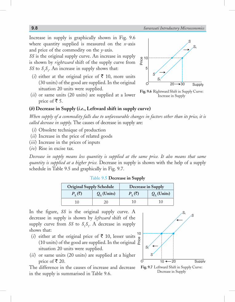
Saraswati Introductory Microeconomics9.8
Increase in supply is graphically shown in Fig. 9.6 where quantity supplied is measured on the x-axis and price of the commodity on the y-axis.SS is the original supply curve. An increase in supply is shown by rightward shift of the supply curve from SS to S1S1. An increase in supply shows that:
(i) either at the original price of ` 10, more units (30 units) of the good are supplied. In the original situation 20 units were supplied.
(ii) or same units (20 units) are supplied at a lower price of ` 5.
(b) Decrease in Supply (i.e., Leftward shift in supply curve)
When supply of a commodity falls due to unfavourable changes in factors other than its price, it is called decrease in supply. The causes of decrease in supply are: (i) Obsolete technique of production (ii) Increase in the price of related goods (iii) Increase in the prices of inputs (iv) Rise in excise tax.
Decrease in supply means less quantity is supplied at the same price. It also means that same quantity is supplied at a higher price. Decrease in supply is shown with the help of a supply schedule in Table 9.5 and graphically in Fig. 9.7.
Table 9.5 Decrease in Supply
Original Supply Schedule Decrease in Supply
PX (`) QX (Units) PX (`) QX (Units)
10 20 10 10
In the figure, SS is the original supply curve. A decrease in supply is shown by leftward shift of the supply curve from SS to S1S1. A decrease in supply shows that: (i) either at the original price of ` 10, lesser units
(10 units) of the good are supplied. In the original situation 20 units were supplied.
(ii) or same units (20 units) are supplied at a higher price of ` 20.
The difference in the causes of increase and decrease in the supply is summarised in Table 9.6.
Fig. 9.7 Leftward Shift in Supply Curve: Decrease in Supply
Fig. 9.6 Rightward Shift in Supply Curve: Increase in Supply
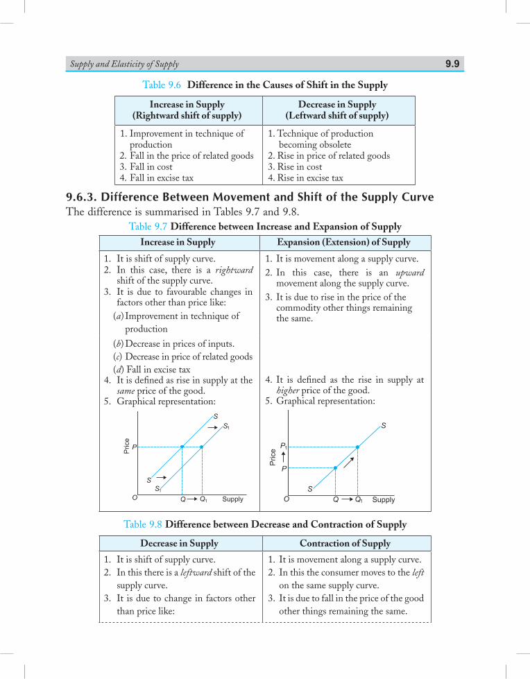
Supply and Elasticity of Supply 9.9
Table 9.6 Difference in the Causes of Shift in the Supply
Increase in Supply (Rightward shift of supply)
Decrease in Supply(Leftward shift of supply)
1. Improvement in technique of production2. Fall in the price of related goods3. Fall in cost4. Fall in excise tax
1. Technique of production becoming obsolete
2. Rise in price of related goods3. Rise in cost4. Rise in excise tax
9.6.3. Difference Between Movement and Shift of the Supply CurveThe difference is summarised in Tables 9.7 and 9.8.
Table 9.7 Difference between Increase and Expansion of SupplyIncrease in Supply Expansion (Extension) of Supply
1. It is shift of supply curve.2. In this case, there is a rightward
shift of the supply curve.3. It is due to favourable changes in
factors other than price like:(a) Improvement in technique of
production
1. It is movement along a supply curve.2. In this case, there is an upward
movement along the supply curve.3. It is due to rise in the price of the
commodity other things remaining the same.
(b) Decrease in prices of inputs.(c) Decrease in price of related goods(d) Fall in excise tax
4. It is defined as rise in supply at the same price of the good.
5. Graphical representation:
4. It is defined as the rise in supply at higher price of the good.
5. Graphical representation:
Table 9.8 Difference between Decrease and Contraction of Supply
Decrease in Supply Contraction of Supply
1. It is shift of supply curve.2. In this there is a leftward shift of the
supply curve.3. It is due to change in factors other
than price like:
1. It is movement along a supply curve.2. In this the consumer moves to the left
on the same supply curve.3. It is due to fall in the price of the good
other things remaining the same.
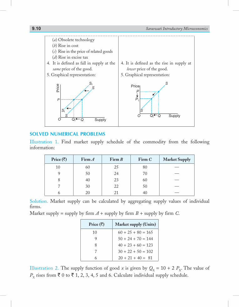
Saraswati Introductory Microeconomics9.10
(a) Obsolete technology(b) Rise in cost(c) Rise in the price of related goods(d) Rise in excise tax
4. It is defined as fall in supply at the same price of the good.
5. Graphical representation:
4. It is defined as the rise in supply at lower price of the good.
5. Graphical representation:
SOLVED NUMERICAL PROBLEMSIllustration 1. Find market supply schedule of the commodity from the following information:
Price (`) Firm A Firm B Firm C Market Supply
109876
6050403020
2524232221
8070605040
—————
Solution. Market supply can be calculated by aggregating supply values of individual firms.Market supply = supply by firm A + supply by firm B + supply by firm C.
Price (`) Market supply (Units)
109876
60 + 25 + 80 = 16550 + 24 + 70 = 14440 + 23 + 60 = 12330 + 22 + 50 = 10220 + 21 + 40 = 81
Illustration 2. The supply function of good x is given by QX = 10 + 2 PX. The value of PX rises from ` 0 to ` 1, 2, 3, 4, 5 and 6. Calculate individual supply schedule.
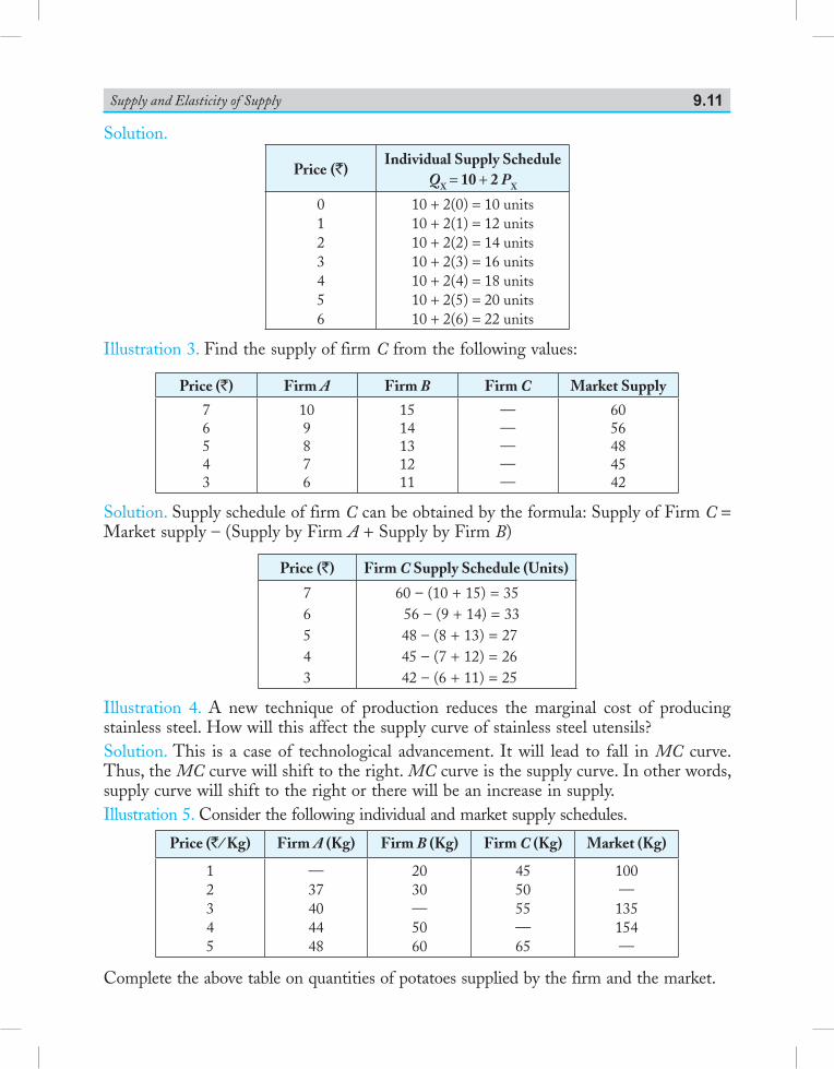
Supply and Elasticity of Supply 9.11
Solution.
Price (`)Individual Supply Schedule
QX = 10 + 2 PX
0123456
10 + 2(0) = 10 units10 + 2(1) = 12 units10 + 2(2) = 14 units10 + 2(3) = 16 units10 + 2(4) = 18 units10 + 2(5) = 20 units10 + 2(6) = 22 units
Illustration 3. Find the supply of firm C from the following values:
Price (`) Firm A Firm B Firm C Market Supply
76543
109876
1514131211
—————
6056484542
Solution. Supply schedule of firm C can be obtained by the formula: Supply of Firm C = Market supply – (Supply by Firm A + Supply by Firm B)
Price (`) Firm C Supply Schedule (Units)
76543
60 – (10 + 15) = 35 56 – (9 + 14) = 33 48 – (8 + 13) = 27 45 – (7 + 12) = 26 42 – (6 + 11) = 25
Illustration 4. A new technique of production reduces the marginal cost of producing stainless steel. How will this affect the supply curve of stainless steel utensils?Solution. This is a case of technological advancement. It will lead to fall in MC curve. Thus, the MC curve will shift to the right. MC curve is the supply curve. In other words, supply curve will shift to the right or there will be an increase in supply.Illustration 5. Consider the following individual and market supply schedules.
Price (`/ Kg) Firm A (Kg) Firm B (Kg) Firm C (Kg) Market (Kg)
12345
—37404448
2030—5060
455055—65
100—135154—
Complete the above table on quantities of potatoes supplied by the firm and the market.
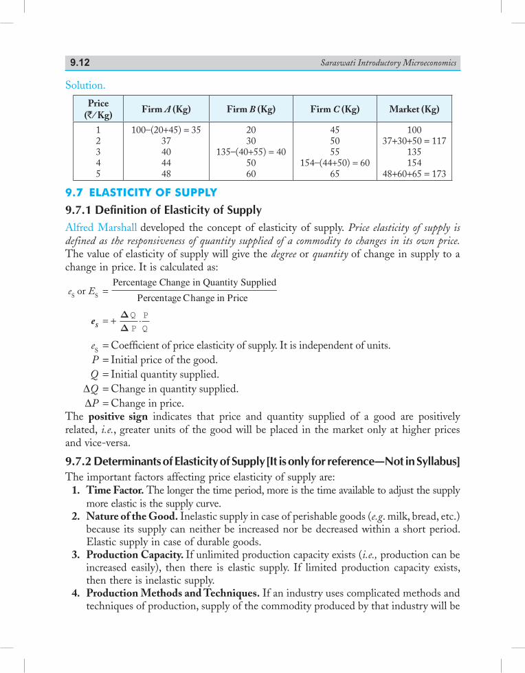
Saraswati Introductory Microeconomics9.12
Solution.
Price (`/ Kg)
Firm A (Kg) Firm B (Kg) Firm C (Kg) Market (Kg)
12345
100–(20+45) = 3537404448
2030
135–(40+55) = 405060
455055
154–(44+50) = 6065
10037+30+50 = 117
135154
48+60+65 = 173
9.7 elaStiCity of Supply
9.7.1 Definition of Elasticity of SupplyAlfred Marshall developed the concept of elasticity of supply. Price elasticity of supply is defined as the responsiveness of quantity supplied of a commodity to changes in its own price. The value of elasticity of supply will give the degree or quantity of change in supply to a change in price. It is calculated as:
eS or ES = Percentage Change in Price
Percentage Change in Quantity Supplied
eS = + DDQP
PQ
.
eS = Coefficient of price elasticity of supply. It is independent of units. P = Initial price of the good. Q = Initial quantity supplied. ΔQ = Change in quantity supplied. ΔP = Change in price.The positive sign indicates that price and quantity supplied of a good are positively related, i.e., greater units of the good will be placed in the market only at higher prices and vice-versa.
9.7.2 Determinants of Elasticity of Supply [It is only for reference—Not in Syllabus]The important factors affecting price elasticity of supply are: 1. Time Factor. The longer the time period, more is the time available to adjust the supply
more elastic is the supply curve. 2. Nature of the Good. Inelastic supply in case of perishable goods (e.g. milk, bread, etc.)
because its supply can neither be increased nor be decreased within a short period. Elastic supply in case of durable goods.
3. Production Capacity. If unlimited production capacity exists (i.e., production can be increased easily), then there is elastic supply. If limited production capacity exists, then there is inelastic supply.
4. Production Methods and Techniques. If an industry uses complicated methods and techniques of production, supply of the commodity produced by that industry will be
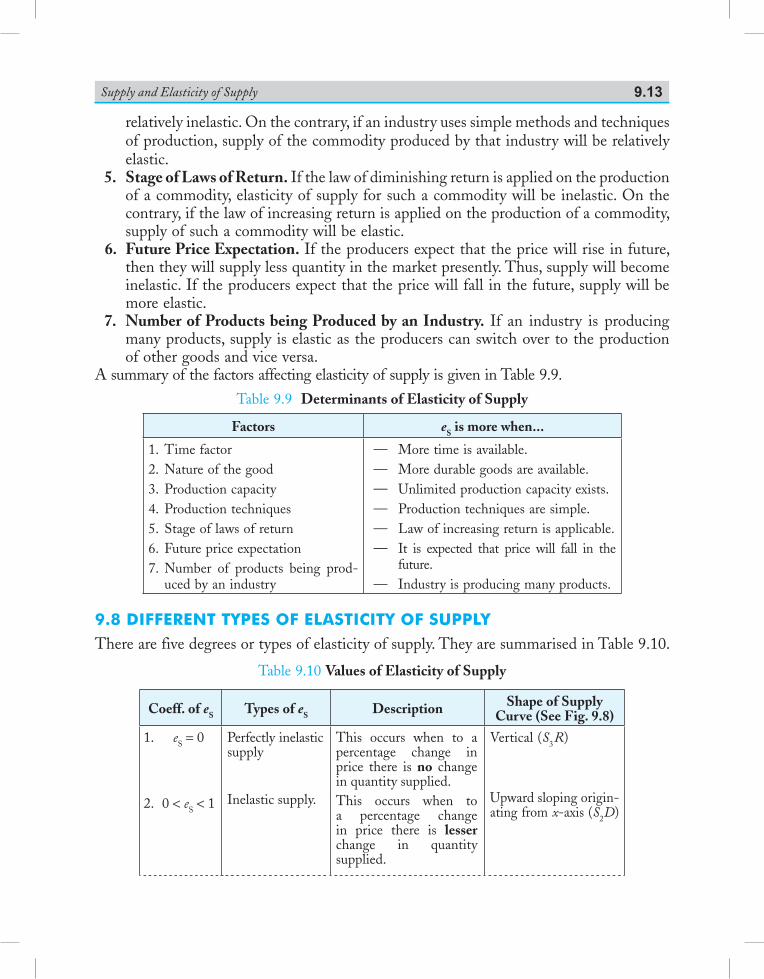
Supply and Elasticity of Supply 9.13
relatively inelastic. On the contrary, if an industry uses simple methods and techniques of production, supply of the commodity produced by that industry will be relatively elastic.
5. Stage of Laws of Return. If the law of diminishing return is applied on the production of a commodity, elasticity of supply for such a commodity will be inelastic. On the contrary, if the law of increasing return is applied on the production of a commodity, supply of such a commodity will be elastic.
6. Future Price Expectation. If the producers expect that the price will rise in future, then they will supply less quantity in the market presently. Thus, supply will become inelastic. If the producers expect that the price will fall in the future, supply will be more elastic.
7. Number of Products being Produced by an Industry. If an industry is producing many products, supply is elastic as the producers can switch over to the production of other goods and vice versa.
A summary of the factors affecting elasticity of supply is given in Table 9.9.Table 9.9 Determinants of Elasticity of Supply
Factors eS is more when...
1. Time factor 2. Nature of the good 3. Production capacity 4. Production techniques 5. Stage of laws of return 6. Future price expectation7. Number of products being prod-
uced by an industry
— More time is available. — More durable goods are available. — Unlimited production capacity exists. — Production techniques are simple. — Law of increasing return is applicable. — It is expected that price will fall in the
future. — Industry is producing many products.
9.8 different typeS of elaStiCity of SupplyThere are five degrees or types of elasticity of supply. They are summarised in Table 9.10.
Table 9.10 Values of Elasticity of Supply
Coeff. of eS Types of eS Description Shape of Supply Curve (See Fig. 9.8)
1. eS = 0
2. 0 < eS < 1
Perfectly inelastic supply
Inelastic supply.
This occurs when to a percentage change in price there is no change in quantity supplied.This occurs when to a percentage change in price there is lesser change in quantity supplied.
Vertical (S3R)
Upward sloping origin-ating from x-axis (S2D)
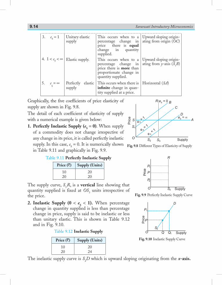
Saraswati Introductory Microeconomics9.14
3. eS = 1
4. 1 < eS < ∞
Unitary elastic supply
Elastic supply.
This occurs when to a percentage change in price there is equal change in quantity supplied.This occurs when to a percentage change in price there is more than proportionate change in quantity supplied.
Upward sloping origin-ating from origin (OC)
Upward sloping origin-ating from y-axis (S1B)
5. eS = ∞ Perfectly elastic
supplyThis occurs when there is infinite change in quan-tity supplied at a price.
Horizontal (SA)
Graphically, the five coefficients of price elasticity of supply are shown in Fig. 9.8.The detail of each coefficient of elasticity of supply with a numerical example is given below:1. Perfectly Inelastic Supply (eS = 0). When supply
of a commodity does not change irrespective of any change in its price, it is called perfectly inelastic supply. In this case, eS = 0. It is numerically shown in Table 9.11 and graphically in Fig. 9.9.
Table 9.11 Perfectly Inelastic Supply
Price (`) Supply (Units)
1020
2020
The supply curve, S3R, is a vertical line showing that quantity supplied is fixed at OS3 units irrespective of the price.
2. Inelastic Supply (0 < eS < 1). When percentage change in quantity supplied is less than percentage change in price, supply is said to be inelastic or less than unitary elastic. This is shown in Table 9.12 and in Fig. 9.10.
Table 9.12 Inelastic Supply
Price (`) Supply (Units)
1020
2024
The inelastic supply curve is S2D which is upward sloping originating from the x-axis.
R
Fig. 9.9 Perfectly Inelastic Supply Curve
Fig. 9.10 Inelastic Supply Curve
R
Fig. 9.8 Different Types of Elasticity of Supply
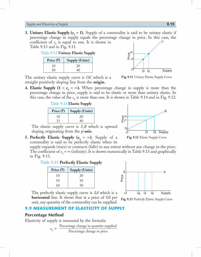
Supply and Elasticity of Supply 9.15
Fig. 9.11 Unitary Elastic Supply Curve
Fig. 9.13 Perfectly Elastic Supply Curve
Fig. 9.12 Elastic Supply Curve
3. Unitary Elastic Supply (eS = 1). Supply of a commodity is said to be unitary elastic if percentage change in supply equals the percentage change in price. In this case, the coefficient of eS is equal to one. It is shown in Table 9.13 and in Fig. 9.11.
Table 9.13 Unitary Elastic Supply
Price (`) Supply (Units)
1020
2040
The unitary elastic supply curve is OC which is a straight positively sloping line from the origin.4. Elastic Supply (1 < eS < ∞). When percentage change in supply is more than the
percentage change in price, supply is said to be elastic or more than unitary elastic. In this case, the value of the eS is more than one. It is shown in Table 9.14 and in Fig. 9.12.
Table 9.14 Elastic Supply
Price (`) Supply (Units)
1011
2040
The elastic supply curve is S1B which is upward sloping originating from the y-axis.
5. Perfectly Elastic Supply (eS = ∞). Supply of a commodity is said to be perfectly elastic when its supply expands (rises) or contracts (falls) to any extent without any change in the price. The coefficient of eS = ∞ (infinity). It is shown numerically in Table 9.15 and graphically in Fig. 9.13.
Table 9.15 Perfectly Elastic Supply
Price (`) Supply (Units)
101010
201030
The perfectly elastic supply curve is SA which is a horizontal line. It shows that at a price of OS per unit, any quantity of the commodity can be supplied.
9.9 meaSurement of elaStiCity of Supply
Percentage MethodElasticity of supply is measured by the formula:
eS = Percentage change in quantity supplied
Percentage change in price
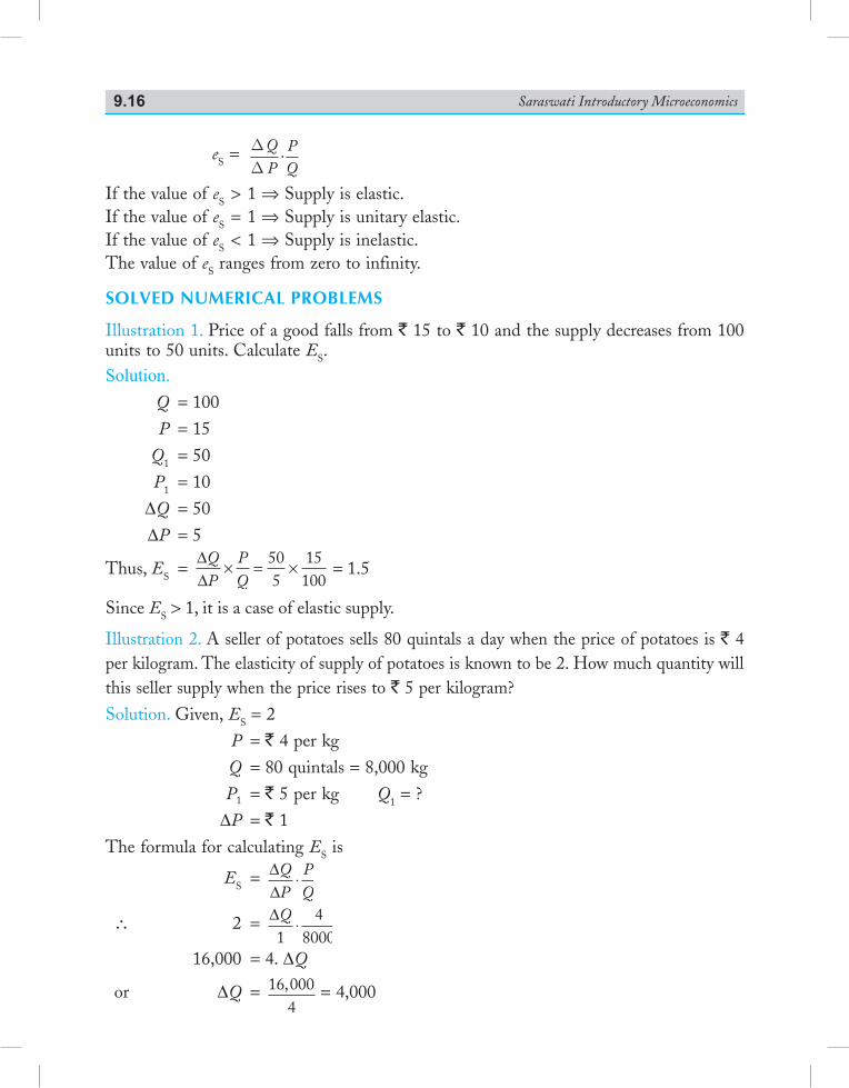
Saraswati Introductory Microeconomics9.16
eS = DD
QP
PQ
.
If the value of eS > 1 ⇒ Supply is elastic. If the value of eS = 1 ⇒ Supply is unitary elastic. If the value of eS < 1 ⇒ Supply is inelastic.The value of eS ranges from zero to infinity.
SOLVED NUMERICAL PROBLEMS
Illustration 1. Price of a good falls from ` 15 to ` 10 and the supply decreases from 100 units to 50 units. Calculate ES.Solution. Q = 100 P = 15 Q1 = 50 P1 = 10 ΔQ = 50 ΔP = 5
Thus, ES = ∆∆
× = × =QP
PQ
505
15100
1 5. = 1.5
Since ES > 1, it is a case of elastic supply.
Illustration 2. A seller of potatoes sells 80 quintals a day when the price of potatoes is ` 4 per kilogram. The elasticity of supply of potatoes is known to be 2. How much quantity will this seller supply when the price rises to ` 5 per kilogram?Solution. Given, ES = 2 P = ` 4 per kg Q = 80 quintals = 8,000 kg P1 = ` 5 per kg Q1 = ? ΔP = ` 1The formula for calculating ES is
ES = ∆∆
⋅QP
PQ
∴ 2 = ∆ ⋅Q1
48000
16,000 = 4. ΔQ
or ΔQ = 16 0004, = 4,000
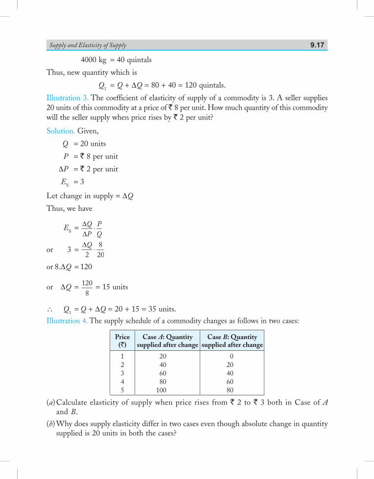
Supply and Elasticity of Supply 9.17
4000 kg = 40 quintals
Thus, new quantity which is
Q1 = Q + ΔQ = 80 + 40 = 120 quintals.
Illustration 3. The coefficient of elasticity of supply of a commodity is 3. A seller supplies 20 units of this commodity at a price of ` 8 per unit. How much quantity of this commodity will the seller supply when price rises by ` 2 per unit?
Solution. Given,
Q = 20 units
P = ` 8 per unit
ΔP = ` 2 per unit
ES = 3
Let change in supply = ΔQ
Thus, we have
ES = ∆∆
⋅QP
PQ
or 3 = ∆ ⋅Q2
820
or 8.ΔQ = 120
or ΔQ = 1208
= 15 units
∴ Q1 = Q + ΔQ = 20 + 15 = 35 units.Illustration 4. The supply schedule of a commodity changes as follows in two cases:
Price (`)
Case A: Quantity supplied after change
Case B: Quantity supplied after change
12345
20406080
100
020406080
(a) Calculate elasticity of supply when price rises from ` 2 to ` 3 both in Case of A and B.
(b) Why does supply elasticity differ in two cases even though absolute change in quantity supplied is 20 units in both the cases?
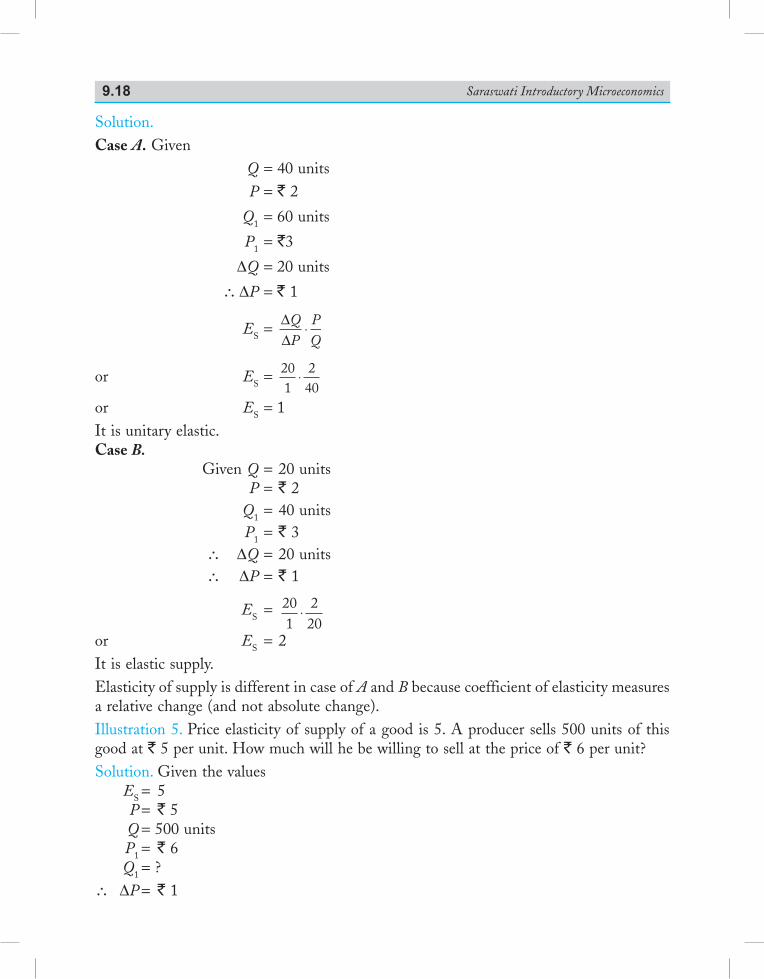
Saraswati Introductory Microeconomics9.18
Solution. Case A. Given Q = 40 units P = ` 2
Q1 = 60 units
P1 = `3
ΔQ = 20 units
∴ ΔP = ` 1
ES = ∆∆
⋅QP
PQ
or ES = 201
240
⋅
or ES = 1It is unitary elastic.Case B. Given Q = 20 units P = ` 2 Q1 = 40 units P1 = ` 3 ∴ ΔQ = 20 units ∴ ΔP = ` 1
ES = 201
220
⋅
or ES = 2It is elastic supply.Elasticity of supply is different in case of A and B because coefficient of elasticity measures a relative change (and not absolute change).Illustration 5. Price elasticity of supply of a good is 5. A producer sells 500 units of this good at ` 5 per unit. How much will he be willing to sell at the price of ` 6 per unit?Solution. Given the values ES = 5 P = ` 5 Q = 500 units P1 = ` 6 Q1 = ?∴ ΔP = ` 1
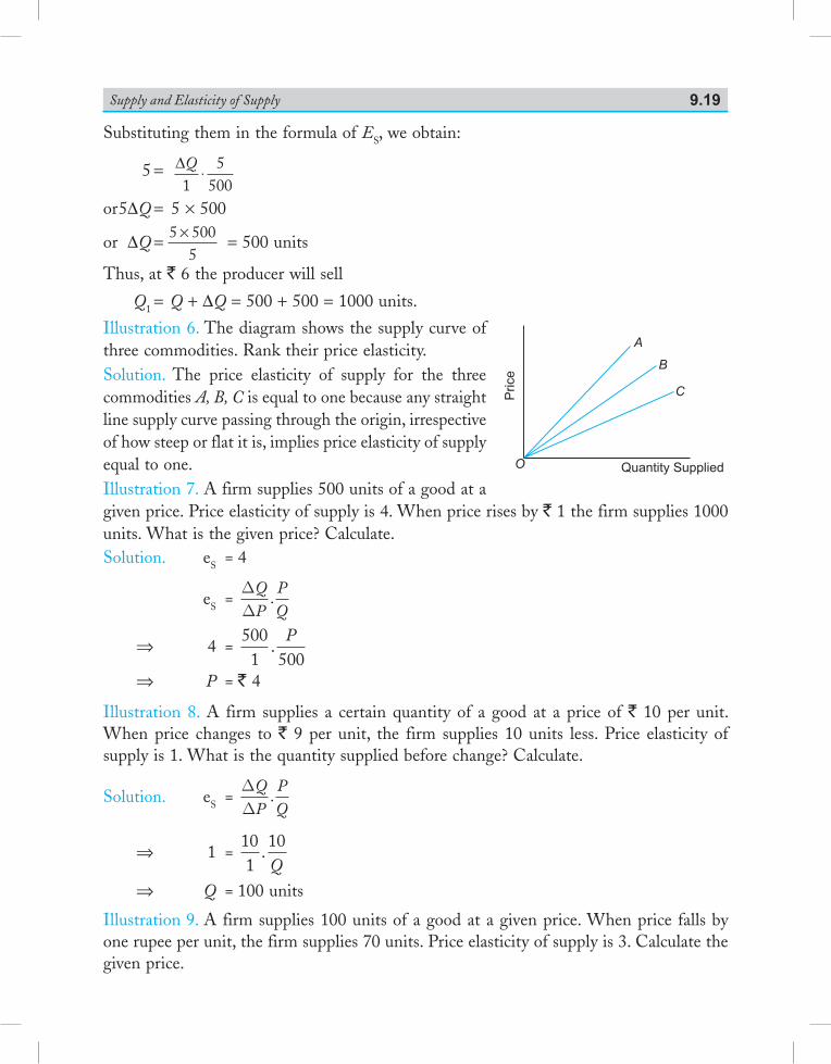
Supply and Elasticity of Supply 9.19
Substituting them in the formula of ES, we obtain:
5 = ∆ ⋅Q1
5500
or 5ΔQ = 5 × 500
or ΔQ = 5 5005
× = 500 units
Thus, at ` 6 the producer will sell
Q1 = Q + ΔQ = 500 + 500 = 1000 units.
Illustration 6. The diagram shows the supply curve of three commodities. Rank their price elasticity.Solution. The price elasticity of supply for the three commodities A, B, C is equal to one because any straight line supply curve passing through the origin, irrespective of how steep or flat it is, implies price elasticity of supply equal to one. Illustration 7. A firm supplies 500 units of a good at a given price. Price elasticity of supply is 4. When price rises by ` 1 the firm supplies 1000 units. What is the given price? Calculate.Solution. eS = 4
eS = DD
QP
PQ
.
⇒ 4 = 5001 500
.P
⇒ P = ` 4
Illustration 8. A firm supplies a certain quantity of a good at a price of ` 10 per unit. When price changes to ` 9 per unit, the firm supplies 10 units less. Price elasticity of supply is 1. What is the quantity supplied before change? Calculate.
Solution. eS = DD
QP
PQ
.
⇒ 1 = 101
10.
Q ⇒ Q = 100 units
Illustration 9. A firm supplies 100 units of a good at a given price. When price falls by one rupee per unit, the firm supplies 70 units. Price elasticity of supply is 3. Calculate the given price.
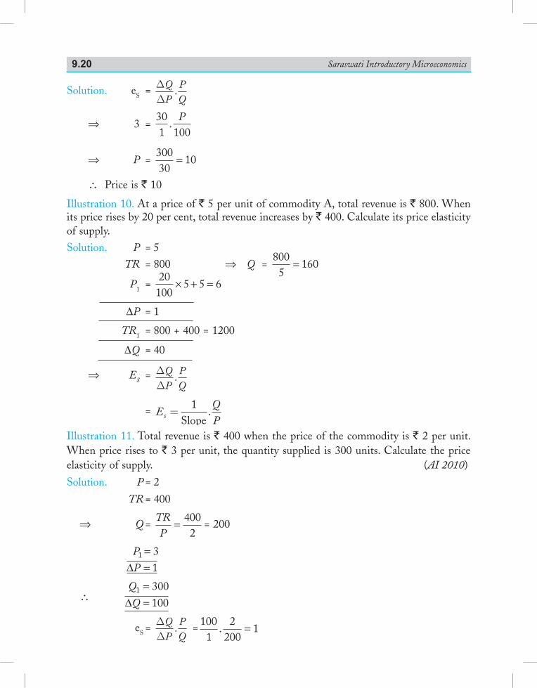
Saraswati Introductory Microeconomics9.20
Solution. eS = DD
QP
PQ
.
⇒ 3 = 301 100
.P
⇒ P = 30030
10=
∴ Price is ` 10
Illustration 10. At a price of ` 5 per unit of commodity A, total revenue is ` 800. When its price rises by 20 per cent, total revenue increases by ` 400. Calculate its price elasticity of supply.Solution. P = 5 TR = 800 ⇒ Q =
8005
160=
P1 = 20
1005 5 6× + =
ΔP = 1
TR1 = 800 + 400 = 1200
ΔQ = 40
⇒ ES = DD
QP
PQ
.
= EQPs =
1Slope
.
Illustration 11. Total revenue is ` 400 when the price of the commodity is ` 2 per unit. When price rises to ` 3 per unit, the quantity supplied is 300 units. Calculate the price elasticity of supply. (AI 2010)
Solution. P = 2
TR = 400
⇒ Q = TRP
= 4002
= 200
P
P1 3
1==∆
∴ Q
Q1 300
100==∆
eS = DD
QP
PQ
. = 1001
2200
1. =
Supply and Elasticity of Supply 9.21
Illustration 12. When the price of a commodity rises by 10 percent, its supply rises by 40 units. Its elasticity of supply is 1. Calculate its supply at the original price. (Delhi 2012) Solution. % change in price = 10 % ΔQ = 40 eS = 1 implies percentage change in quantity supplied is 10%
That is, ∆QQ
× 100 = 10
⇒ 40100
Q× = 10
⇒ Q = 400 units.
Illustration 13. At a price of ` 10 per unit, the supply of a commodity is 300 units. Its elasticity of supply is 1.5. Its price increases by 20 percent. Calculate its supply at the increased price. (AI 2012)Solution. P1 = P + % Δ in P
= 10 + 20
100 × 10 = 12
∴ 1.5 = ΔQ2
. 10300
⇒ ΔQ = 1.5 × 60 = 90 ∴ Q1 = Q + ΔQ = 300 + 90 = 390 units.
Points to RememberSupply 1. Supply of a commodity at a given price is the quantity of the commodity which is actually
offered for sale per unit of time.
2. There is difference between supply and stock. Supply is that part of stock which is actually brought in the market.
Supply Function and its Slope
Symbolically, a supply function can be expressed as:
SX = f (PX, PZ, T, C, GP)
Slope of Supply Curve = ∆∆
⋅QP
PQ
Factors Determining Supply
Factors determining supply of a good are: (i) price of the commodity; (ii) price of the related good (Pz); (iii) cost of production or price of inputs; (C) (iv) state of technology; (T) (v) government policy or excise tax (Gp).
Saraswati Introductory Microeconomics9.22
The Law of Supply
1. The law of supply states that there is a direct relationship between price and quantity supplied of a commodity, other things remaining constant.
2. The assumptions of the law are that PZ, T, C and GP are constant. 3. The supply schedule shows the different quantities of a commodity supplied by a firm within
a given period of time at different prices. 4. The data of supply schedule is plotted on price and quantity axes to derive the supply curve.
The supply curve is upward sloping because of: (i) law of diminishing marginal productivity (ii) goal of profit maximisation. 5. In the market period or very short period, supply curve is a vertical line.From Individual Supply to Market Supply
1. Individual supply is the supply on the part of a single producer at various prices per time period. Market supply is the aggregate of the quantity supplied by all the producers at various prices per time period.
2. Market supply curve is constructed by horizontal summation of individual supply curves.
Change in Quantity Supplied (Movement) vs Change in Supply (Shift) 1. Movement along a supply curve occurs due to changes in the price of good (PX) itself. Shift
to the supply curve occurs due to changes in PZ, T, C or GP . 2. Movement can be expansion (extension) or contraction of supply whereas shift can be
increase or decrease in supply.Elasticity of Supply (eS) 1. The concept of eS was developed by Marshall. Elasticity of supply is defined as the
responsiveness of quantity supplied of a good to changes in its own price. Symbolically,
eS = ∆∆
⋅QP
PQ
2. The major determinants of elasticity of supply are: (i) time factor; (ii) nature of the good; (iii) production capacity; (iv) production techniques; (v) stage of laws of return; (vi) future price expectation; (vii) number of products being produced by the industry.
Different Types or Degrees of Elasticity of Supply
There are five degrees of eS: (i) Perfectly Inelastic Supply (eS = 0) (ii) Inelastic Supply (0 < eS < 1) (iii) Unitary Elastic Supply (eS = 1) (iv) Elastic Supply (1 < eS < ∞) (v) Perfectly Elastic Supply (eS = ∞)
Measurement of Elasticity of Supply
Percentage Method
Elasticity of supply is me asured by the formula:
eS = Percentage change in quantity suppliedPercentage change in price
= ∆∆
⋅QP
PQ
Supply and Elasticity of Supply 9.23
Test Your KnowledgeVery Short Answer Type Questions (1 Mark) 1. Define supply. (Delhi 2011,12) 2. What is meant by a change in supply? (Delhi 2012) 3. Define price elasticity of supply. 4. Draw a straight line supply curve with infinite price elasticity. 5. Give meaning of “Change in quantity supplied”. (Foreign 2011) 6. What is meant by ‘increase in supply’? (Delhi 2011) 7. What is ‘decrease in supply’? (Delhi 2011) 8. Define market supply. (Delhi 2012; AI, Foreign 2013) 9. When does a supply curve shift? (Delhi 2012) 10. Give one reason for an “increase” in supply of a commodity. (AI 2013) 11. Give one reason for “decrease” in supply of a commodity. (AI 2013) 12. When is supply of a good said to be inelastic? (Foreign 2013) 13. When does ‘increase’ in supply take place? (Delhi 2016) 14. When does ‘decrease’ in supply take place? (Delhi 2016) 15. When does ‘shift’ in supply curve take place? (AI 2016)
Multiple Choice Questions
1. What is constant in the law of supply? (a) Price of related goods (b) State of technology (c) Cost of production (d) All of the above 2. When supply curve is upward sloping, its slope is __________. (a) Positive (b) Negative (c) First positive then negative (d) Zero 3. Market supply curve is ________ summation of individual supply curves. (a) Horizontal (b) Vertical (c) Can be both horizontal or vertical (d) None of the above 4. Movement along the supply curve is also called: (a) Change in supply (b) Change in quantity supplied (c) Contraction in supply (d) Increase in supply 5. An upward movement along a supply curve shows: (a) Contraction in supply (b) Decrease in supply (c) Expansion in supply (d) Increase in supply
6. A rightward shift in supply curve shows: (a) Contraction in supply (b) Decrease in supply (c) Expansion in supply (d) Increase in supply 7. When less quantity is supplied at a lower price, it shows: (a) Contraction in supply (b) Decrease in supply (c) Expansion in supply (d) Increase in supply
Saraswati Introductory Microeconomics9.24
8. When same quantity is supplied at a higher price, it shows: (a) Contraction in supply (b) Decrease in supply (c) Expansion in supply (d) Increase in supply 9. Elasticity of supply is given by the formula:
(a) DD
QP
PQ
. (b) DD
PQ
QP
. (c) DD
QP
QP
. (d) DD
QP
10. Slope of supply curve is given by the formula:
(a) DD
QP
(b) DD
PQ
(c) PQ
(d) QP
11. Relationship between slope and elasticity of supply is:
(a) EPQs =
1Slope
. (b) EQPs =Slope . (c) E
QPs =
1Slope
. (d) Es = Slope
12. The value of elasticity of supply ranges from: (a) Zero to infinity (b) Minus infinity to plus infinity (c) One to infinity (d) Zero to minus infinity. 13. When supply curve is vertical, ES = ____________? (a) Zero (b) 1 (c) ∞ (d) ES > 1 14. When supply curve is horizontal, ES = ___________?
(a) Zero (b) 1 (c) ∞ (d) ES > 1
Short Answer Type Questions (3/4 Marks) 1. Draw supply curves showing price elasticity of supply equal to (Foreign 2012) (i) zero, (ii) one, and (iii) infinity throughout. 2. At a price of ` 5 per unit of commodity A, total revenue is ` 800. When its price rises by 20
per cent, total revenue increases by ` 400. Calculate its price elasticity of supply. [Ans. eS = 1.25] (Delhi 2010) 3. Total revenue is ` 400 when the price of the commodity is ` 2 per unit. When price rises to
` 3 per unit, the quantity supplied is 300 units. Calculate the price elasticity of supply. [Ans. eS = 1] (AI 2010) 4. Define ‘Market Supply’. What is the effect on the supply of a good when Government
imposes a tax on the production of that good? Explain. (Delhi 2011) 5. What is a supply schedule? Explain how does change in technology of producing a good
affect the supply of that good. (Foreign 2011) 6. Explain how changes in prices of other products influence the supply of a given product. (Delhi 2012, 14)
7. Explain how changes in prices of inputs influence the supply of a product. (AI 2012) 8. How does the change in tax on a product influence the supply of that product? Explain. (Foreign 2012, 14) 9. When the price of a commodity rises by 10 percent, its supply rises by 40 units. Its elasticity
of supply is 1. Calculate its supply at the original price. [Ans. 400 units] (Delhi 2012)
Supply and Elasticity of Supply 9.25
10. The price of a commodity falls by 15 percent and its supply falls from 200 units to 155 units. Calculate its elasticity of supply. [Ans. eS = 1.5] (Delhi 2012)
11. Price elasticity of supply of a commodity is 1. Its price rises from ` 20 to ` 24 per unit and its supply rises by 300 units. Calculate its supply at the original price of ` 20 per unit.
[Ans. 1500 units] (AI 2012)
12. At a price of ` 10 per unit, the supply of a commodity is 300 units. Its elasticity of supply is 1.5. Its price increases by 20 percent. Calculate its supply at the increased price.
[Ans. 390 units] (AI 2012) 13. When the price of a good rises from ` 20 per unit to ` 30 per unit, the revenue of the firm
producing this good rises from ` 100 to ` 300. Calculate the price elasticity of supply. [Ans. 2](Delhi 2013) 14. A firm’s revenue rises from ` 400 to ` 500 when the price of its product rises from ` 20 per
unit to ` 25 per unit. Calculate the price elasticity of supply. [Ans. 0](Delhi 2013) 15. The price elasticity of supply of a good is 0.8. Its price rises by 50 percent. Calculate the
percentage increase in its supply. [Ans. 40%] (Delhi 2013) 16. The price elasticity of supply of a commodity is 2.0. A firm supplies 200 units of it at a price
of ` 8 per unit. At what price will it supply 250 units? [Ans. ` 9] (AI 2013) 17. A 15 percent rise in the price of a commodity raises its supply from 300 units to 345 units.
Calculate its price elasticity of supply. [Ans. 1](AI 2013) 18. Total revenue of a firm rises from ` 400 to ` 500 when the price of its product rises from ` 8
per unit to ` 10 per unit. Calculate the price elasticity of supply. [Ans. 0] (Foreign 2013) 19. Price elasticity of supply of a good is 2. By what percentage should its price rise so that its
supply rises by 30 percent? [Ans. 15%](Foreign 2013) 20. Explain how technological progress is a determinant of supply of a good by a firm. (AI 2014) 21. How does subsidy influence the supply of a good by a firm? Explain (Foreign 2014) 22. What is supply? Explain the effect of technological progress on supply of a good. (Foreign 2015)
or What is ‘change in supply’? Explain the effect of tax imposed on a good on the supply of the
good. (Foreign 2015) 23. When price of a commodity falls from ` 12 per unit to ` 9 per unit, the producer supplies
75 per cent less output. Calculate price elasticity of supply. [Ans. ES = 3] (AI 2016) 24. What is perfectly elastic supply? When price falls by ` 2 per unit, supply falls from 100 units
to 80 units. Price elastic of supply is 2. What was the price per unit before change? Calculate. [Ans. ` = 20] (Foreign 2016)
25. Price elasticity of supply of a good is 2. A producer supplies 100 units of a good at a price of ` 20 per unit. At what price will he supply 80 units. [Ans. ` = 18] (Delhi 2016)
26. When price of a good rises from ` 10 to ` 12 per unit, the producer supplies 10 per cent more. Calculate price elasticity of supply. [Ans. ES = 0.5] (AI 2016)
27. When price of a good rises from ` 12 per unit to ` 15 per unit the producer supplies 50 per cent more output. What is the price elasticity of supply? Calculate.
[Ans. ES = 2] (Delhi 2016)
Saraswati Introductory Microeconomics9.26
28. When price of a good rises from ` 8 per unit to ` 10 per unit, producer supplies 40 units more. Price elasticity of supply is 2. What is the quantity supplied before the price change? Calculate. [Ans. Q = 80] (AI 2016)
29. A producer supplies 80 units of a good at a price of ` 10 per unit. Price elasticity of supply is 4. How much will he supply at ` 9 per unit? [Ans. 48 units] (Delhi 2016)
30. Explain the geometric method of measuring price elasticity of supply. Use Diagram. (Delhi 2017)
31. Define market supply. Explain the factor ‘input prices’ that can cause a change in supply. (AI 2017)
Long Answer Type Questions (6 Marks)
1. Given eS = 5, original price = ` 60, new price = ` 100, change in quantity = 20 units. Find the original quantity and the new quantity supplied. [Ans. Q = 6 units, Q
1 = 26 units]
2. The coefficient of ES of a good is 8. A seller supplies 36 units of this good at a price of ` 6 per unit. How much quantity of this good will this seller supply when price rises by ` 10 per unit? [Ans. 516 units]
3. Price elasticity of supply of a good is 2. A producer sells 200 units of this good at ` 2 per unit. How much will he be willing to sell at the price of ` 4 per unit? [Ans. 600 units]
4. Given eS = 2. A producer sells 10 units of a good at ` 4. How much will he be willing to sell at a price of ` 5 per unit? [Ans. 15 units]
5. A producer sells 40 units of a good at a price of ` 2. If price rises to ` 4, he sells 80 units of a good. Calculate eS. [Ans. eS = 1]
6. A good has a unitary elastic supply. If the producer sells 40 units of that good at a price of ` 2, how much will he be willing to sell at a price of ` 3? [Ans. 60 units]
7. Explain any three causes of “increase” in supply of a commodity. (Delhi 2012) 8. Explain any two causes of “decrease” in supply of a good. (AI 2012) 9. Explain the distinction between “change in quantity supplied” and “change in supply”. Use
diagram. (AI 2012) 10. Explain the distinction between “decrease in supply” and “contraction in supply”. Use
diagrams. (Foreign 2013) 11. Explain the distinction between “movement along the supply curve” and “shift of supply
curve”. Use diagrams. (Foreign 2013) 12. Explain the distinction between “change in quantity supplied” and “change in supply”. Use
diagram. (Delhi 2016) 13. Examine the effect of (i) fall in the own price of good X and (ii) rise in tax rate on good X,
on the supply curve. Use diagrams. (AI 2016)
AnswersMultiple Choice Questions
1. (d) 2. (a) 3. (a) 4. (b) 5. (c) 6. (d) 7. (a) 8. (b)
9. (a) 10. (b) 11. (a) 12. (a) 13. (a) 14. (c)
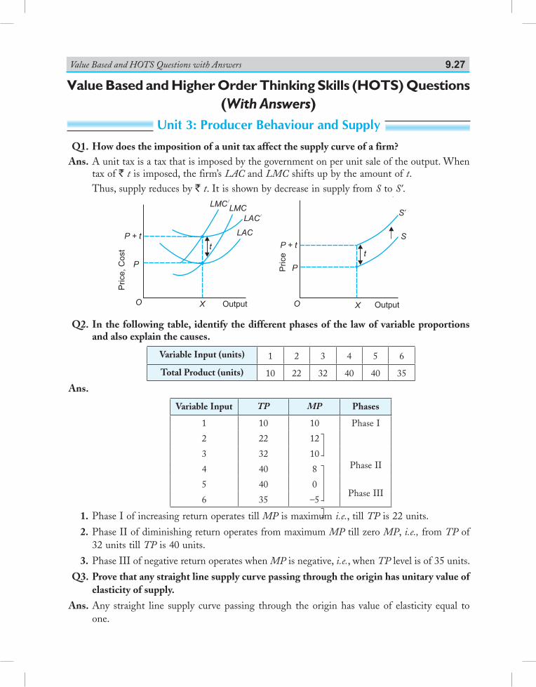
Value Based and HOTS Questions with Answers 9.27
Value Based and Higher Order Thinking Skills (HOTS) Questions(With Answers)
Unit 3: Producer Behaviour and Supply Q1. How does the imposition of a unit tax affect the supply curve of a firm? Ans. A unit tax is a tax that is imposed by the government on per unit sale of the output. When
tax of ` t is imposed, the firm’s LAC and LMC shifts up by the amount of t. Thus, supply reduces by ` t. It is shown by decrease in supply from S to S’.
Price,C
ost
Price,C
ost
Q2. In the following table, identify the different phases of the law of variable proportions and also explain the causes.
Variable Input (units) 1 2 3 4 5 6
Total Product (units) 10 22 32 40 40 35
Ans.
Variable Input TP MP Phases
1 10 10 Phase I
Phase II
Phase III
2 22 12
3 32 10
4 40 8
5 40 0
6 35 –5
1. Phase I of increasing return operates till MP is maximum i.e., till TP is 22 units.
2. Phase II of diminishing return operates from maximum MP till zero MP, i.e., from TP of 32 units till TP is 40 units.
3. Phase III of negative return operates when MP is negative, i.e., when TP level is of 35 units.
Q3. Prove that any straight line supply curve passing through the origin has unitary value of elasticity of supply.
Ans. Any straight line supply curve passing through the origin has value of elasticity equal to one.
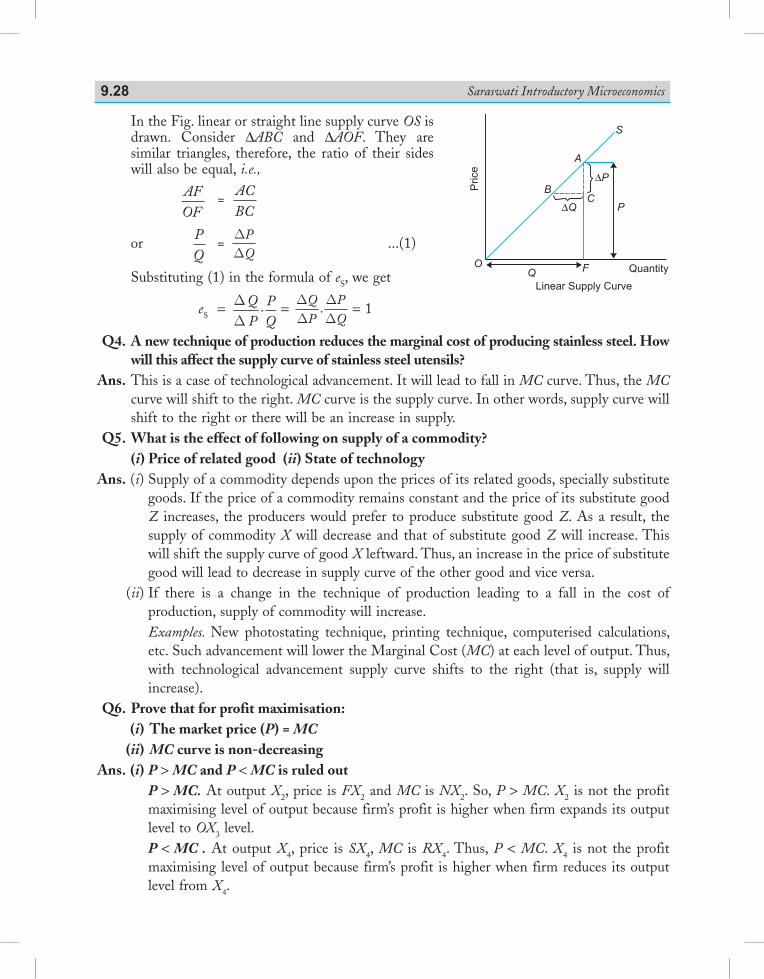
Saraswati Introductory Microeconomics9.28
In the Fig. linear or straight line supply curve OS is drawn. Consider ΔABC and ΔAOF. They are similar triangles, therefore, the ratio of their sides will also be equal, i.e.,
AFOF
= ACBC
or PQ
= DD
PQ
...(1)
Substituting (1) in the formula of eS, we get
eS = DD
QP
PQ
. = DD
DD
QP
PQ
. = 1
Q4. A new technique of production reduces the marginal cost of producing stainless steel. How will this affect the supply curve of stainless steel utensils?
Ans. This is a case of technological advancement. It will lead to fall in MC curve. Thus, the MC curve will shift to the right. MC curve is the supply curve. In other words, supply curve will shift to the right or there will be an increase in supply.
Q5. What is the effect of following on supply of a commodity? (i) Price of related good (ii) State of technology Ans. (i) Supply of a commodity depends upon the prices of its related goods, specially substitute
goods. If the price of a commodity remains constant and the price of its substitute good Z increases, the producers would prefer to produce substitute good Z. As a result, the supply of commodity X will decrease and that of substitute good Z will increase. This will shift the supply curve of good X leftward. Thus, an increase in the price of substitute good will lead to decrease in supply curve of the other good and vice versa.
(ii) If there is a change in the technique of production leading to a fall in the cost of production, supply of commodity will increase.
Examples. New photostating technique, printing technique, computerised calculations, etc. Such advancement will lower the Marginal Cost (MC) at each level of output. Thus, with technological advancement supply curve shifts to the right (that is, supply will increase).
Q6. Prove that for profit maximisation: (i) The market price (P) = MC (ii) MC curve is non-decreasing Ans. (i) P > MC and P < MC is ruled out P > MC. At output X2, price is FX2 and MC is NX2. So, P > MC. X2 is not the profit
maximising level of output because firm’s profit is higher when firm expands its output level to OX3 level.
P < MC . At output X4, price is SX4, MC is RX4. Thus, P < MC. X4 is not the profit maximising level of output because firm’s profit is higher when firm reduces its output level from X4.
Price
OQ
F Quantity
P∆QC
B
A
S
∆P
Linear Supply Curve
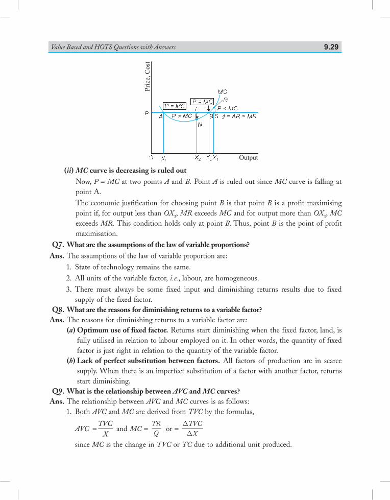
Value Based and HOTS Questions with Answers 9.29
Pri
ce,C
ost
Output
(ii) MC curve is decreasing is ruled out Now, P = MC at two points A and B. Point A is ruled out since MC curve is falling at
point A. The economic justification for choosing point B is that point B is a profit maximising
point if, for output less than OX3, MR exceeds MC and for output more than OX3, MC exceeds MR. This condition holds only at point B. Thus, point B is the point of profit maximisation.
Q7. What are the assumptions of the law of variable proportions? Ans. The assumptions of the law of variable proportion are: 1. State of technology remains the same. 2. All units of the variable factor, i.e., labour, are homogeneous. 3. There must always be some fixed input and diminishing returns results due to fixed
supply of the fixed factor. Q8. What are the reasons for diminishing returns to a variable factor? Ans. The reasons for diminishing returns to a variable factor are: (a) Optimum use of fixed factor. Returns start diminishing when the fixed factor, land, is
fully utilised in relation to labour employed on it. In other words, the quantity of fixed factor is just right in relation to the quantity of the variable factor.
(b) Lack of perfect substitution between factors. All factors of production are in scarce supply. When there is an imperfect substitution of a factor with another factor, returns start diminishing.
Q9. What is the relationship between AVC and MC curves? Ans. The relationship between AVC and MC curves is as follows: 1. Both AVC and MC are derived from TVC by the formulas,
AVC =TVC
Xand MC =
TRQ
or = DDTVC
X
since MC is the change in TVC or TC due to additional unit produced.
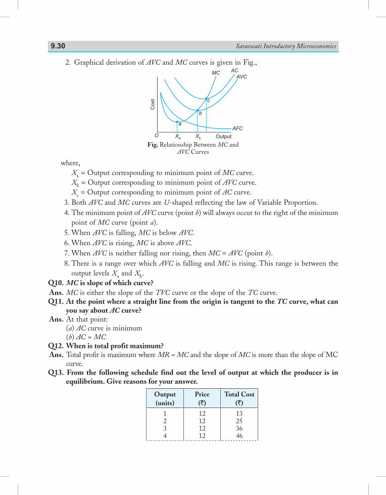
Saraswati Introductory Microeconomics9.30
2. Graphical derivation of AVC and MC curves is given in Fig.,
Fig. Relationship Between MC and AVC Curves
O
AVC
AFC
Co
st
Output
MCAC
a
b
c
Xa
Xb
where, Xa = Output corresponding to minimum point of MC curve. Xb = Output corresponding to minimum point of AVC curve. Xc = Output corresponding to minimum point of AC curve. 3. Both AVC and MC curves are U-shaped reflecting the law of Variable Proportion. 4. The minimum point of AVC curve (point b) will always occur to the right of the minimum
point of MC curve (point a). 5. When AVC is falling, MC is below AVC. 6. When AVC is rising, MC is above AVC. 7. When AVC is neither falling nor rising, then MC = AVC (point b). 8. There is a range over which AVC is falling and MC is rising. This range is between the
output levels Xa and Xb.Q10. MC is slope of which curve? Ans. MC is either the slope of the TVC curve or the slope of the TC curve.Q11. At the point where a straight line from the origin is tangent to the TC curve, what can
you say about AC curve? Ans. At that point: (a) AC curve is minimum (b) AC = MC
Q12. When is total profit maximum? Ans. Total profit is maximum where MR = MC and the slope of MC is more than the slope of MC
curve. Q13. From the following schedule find out the level of output at which the producer is in
equilibrium. Give reasons for your answer.
Output (units)
Price(`)
Total Cost(`)
1234
12121212
13253646
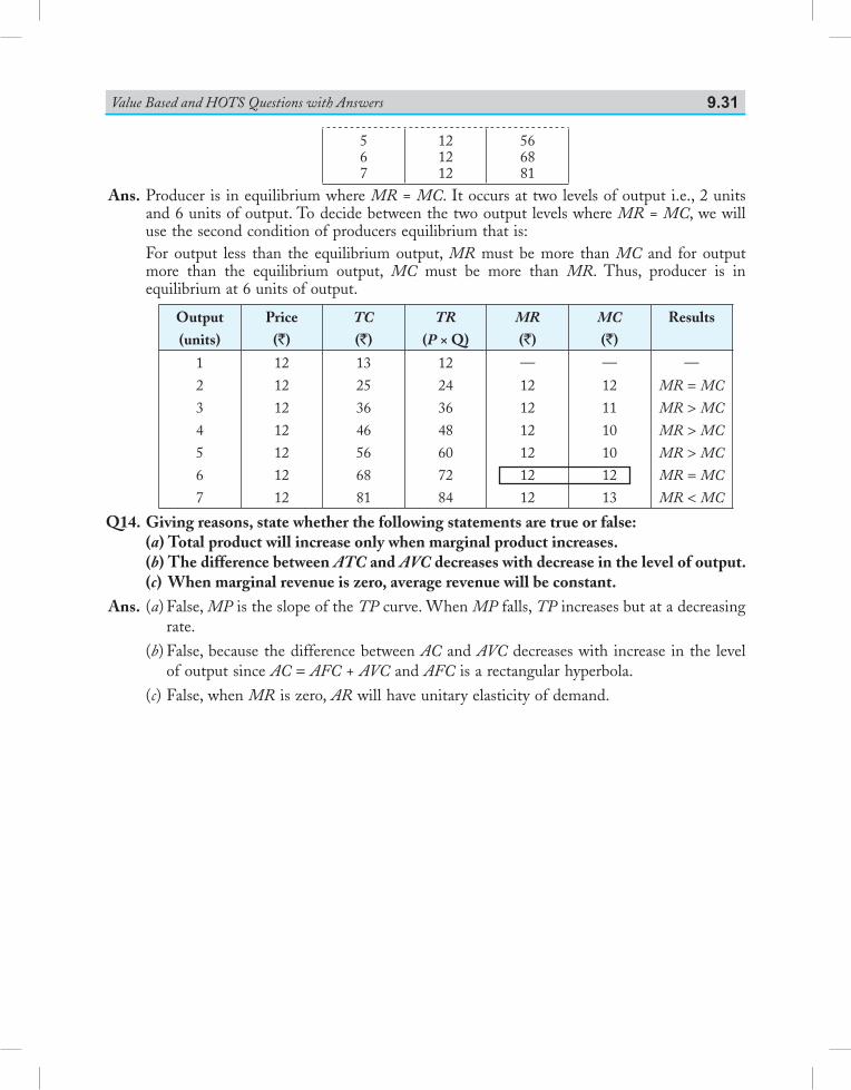
Value Based and HOTS Questions with Answers 9.31
567
121212
566881
Ans. Producer is in equilibrium where MR = MC. It occurs at two levels of output i.e., 2 units and 6 units of output. To decide between the two output levels where MR = MC, we will use the second condition of producers equilibrium that is:
For output less than the equilibrium output, MR must be more than MC and for output more than the equilibrium output, MC must be more than MR. Thus, producer is in equilibrium at 6 units of output.
Output (units)
Price(`)
TC
(`)TR
(P × Q)MR
(`)MC
(`)Results
1
2
3
4
5
6
7
12
12
12
12
12
12
12
13
25
36
46
56
68
81
12
24
36
48
60
72
84
—
12
12
12
12
12
12
—
12
11
10
10
12
13
—
MR = MC
MR > MC
MR > MC
MR > MC
MR = MC
MR < MC
Q14. Giving reasons, state whether the following statements are true or false: (a) Total product will increase only when marginal product increases. (b) The difference between ATC and AVC decreases with decrease in the level of output. (c) When marginal revenue is zero, average revenue will be constant.
Ans. (a) False, MP is the slope of the TP curve. When MP falls, TP increases but at a decreasing rate.
(b) False, because the difference between AC and AVC decreases with increase in the level of output since AC = AFC + AVC and AFC is a rectangular hyperbola.
(c) False, when MR is zero, AR will have unitary elasticity of demand.
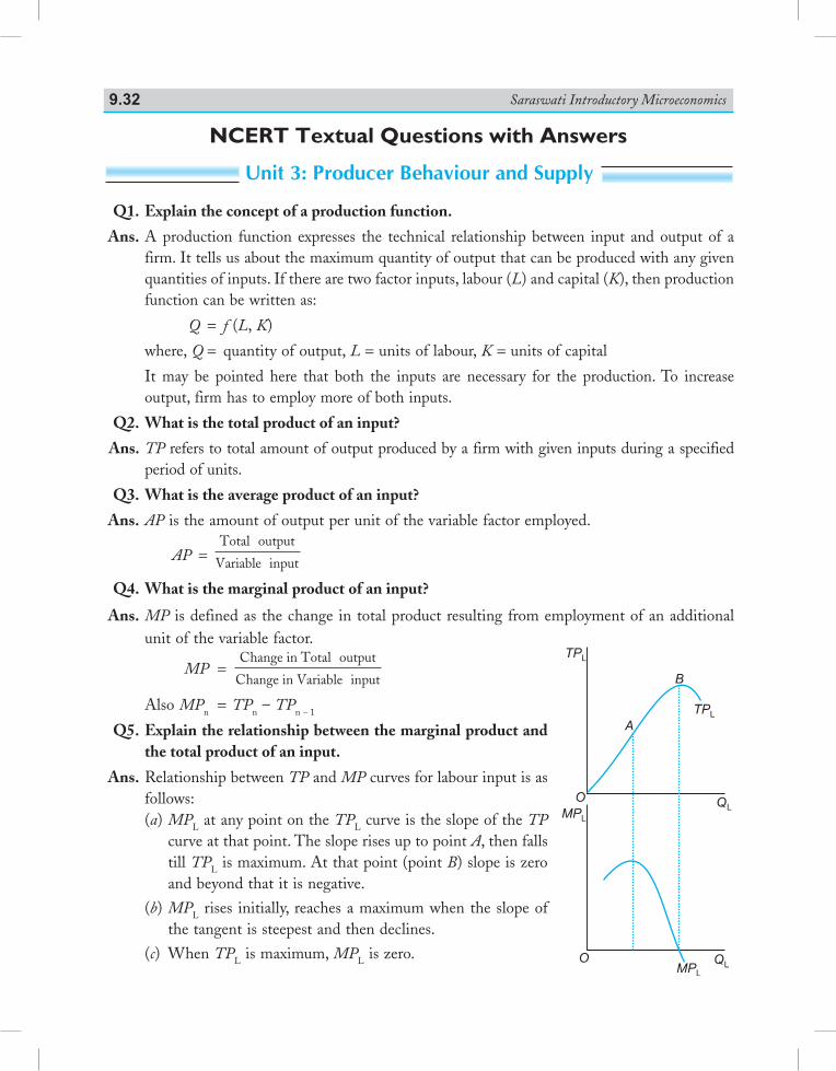
Saraswati Introductory Microeconomics9.32
Unit 3: Producer Behaviour and Supply
Q1. Explain the concept of a production function.
Ans. A production function expresses the technical relationship between input and output of a firm. It tells us about the maximum quantity of output that can be produced with any given quantities of inputs. If there are two factor inputs, labour (L) and capital (K), then pro duc tion function can be written as:
Q = f (L, K)
where, Q = quantity of output, L = units of labour, K = units of capital
It may be pointed here that both the inputs are necessary for the production. To increase output, firm has to employ more of both inputs.
Q2. What is the total product of an input?
Ans. TP refers to total amount of output produced by a firm with given inputs during a spec i fied period of units.
Q3. What is the average product of an input?
Ans. AP is the amount of output per unit of the variable factor employed.
AP = Total output
Variable input
Q4. What is the marginal product of an input?
Ans. MP is defined as the change in total product resulting from employment of an additional unit of the variable factor.
MP = Change in Total output
Change in Variable input
Also MPn = TPn – TPn – 1
Q5. Explain the relationship between the marginal product and the total product of an input.
Ans. Relationship between TP and MP curves for labour input is as follows:(a) MPL at any point on the TPL curve is the slope of the TP
curve at that point. The slope rises up to point A, then falls till TPL is maximum. At that point (point B) slope is zero and beyond that it is negative.
(b) MPL rises initially, reaches a maximum when the slope of the tangent is steepest and then declines.
(c) When TPL is maximum, MPL is zero.
NCERT Textual Questions with Answers
Q
Q
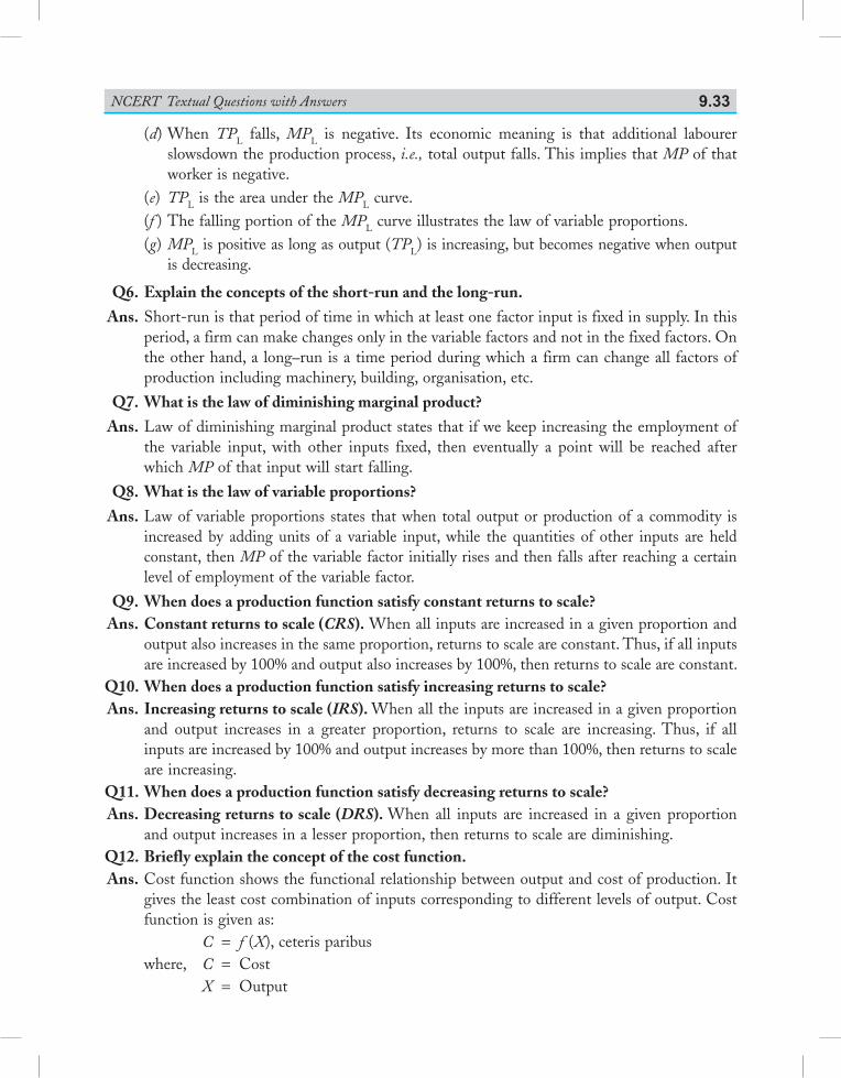
NCERT Textual Questions with Answers 9.33
(d) When TPL falls, MPL is negative. Its economic meaning is that additional labourer slowsdown the production process, i.e., total output falls. This implies that MP of that worker is negative.
(e) TPL is the area under the MPL curve.(f ) The falling portion of the MPL curve illustrates the law of variable proportions.(g) MPL is positive as long as output (TPL) is increasing, but becomes negative when output
is decreasing.
Q6. Explain the concepts of the short-run and the long-run. Ans. Short-run is that period of time in which at least one factor input is fixed in supply. In this
period, a firm can make changes only in the variable factors and not in the fixed factors. On the other hand, a long–run is a time period during which a firm can change all factors of production including machinery, building, organisation, etc.
Q7. What is the law of diminishing marginal product? Ans. Law of diminishing marginal product states that if we keep increasing the employment of
the variable input, with other inputs fixed, then eventually a point will be reached after which MP of that input will start falling.
Q8. What is the law of variable proportions? Ans. Law of variable proportions states that when total output or production of a commodity is
increased by adding units of a variable input, while the quantities of other inputs are held constant, then MP of the variable factor initially rises and then falls after reaching a certain level of employment of the variable factor.
Q9. When does a production function satisfy constant returns to scale? Ans. Constant returns to scale (CRS). When all inputs are increased in a given proportion and
output also increases in the same proportion, returns to scale are constant. Thus, if all inputs are increased by 100% and output also increases by 100%, then returns to scale are constant.
Q10. When does a production function satisfy increasing returns to scale? Ans. Increasing returns to scale (IRS). When all the inputs are increased in a given proportion
and output increases in a greater proportion, returns to scale are increasing. Thus, if all inputs are increased by 100% and output increases by more than 100%, then returns to scale are increasing.
Q11. When does a production function satisfy decreasing returns to scale? Ans. Decreasing returns to scale (DRS). When all inputs are increased in a given proportion
and output increases in a lesser proportion, then returns to scale are diminishing. Q12. Briefly explain the concept of the cost function. Ans. Cost function shows the functional relationship between output and cost of production. It
gives the least cost combination of inputs corresponding to different levels of output. Cost function is given as:
C = f (X), ceteris paribus where, C = Cost X = Output
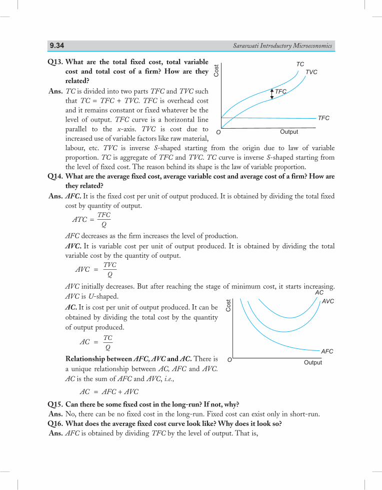
Saraswati Introductory Microeconomics9.34
Q13. What are the total fixed cost, total variable cost and total cost of a firm? How are they related?
Ans. TC is divided into two parts TFC and TVC such that TC = TFC + TVC. TFC is overhead cost and it remains constant or fixed whatever be the level of output. TFC curve is a horizontal line parallel to the x-axis. TVC is cost due to increased use of variable factors like raw material, labour, etc. TVC is inverse S-shaped starting from the origin due to law of variable proportion. TC is aggregate of TFC and TVC. TC curve is inverse S-shaped starting from the level of fixed cost. The reason behind its shape is the law of variable proportion.
Q14. What are the average fixed cost, average variable cost and average cost of a firm? How are they related?
Ans. AFC. It is the fixed cost per unit of output produced. It is obtained by dividing the total fixed cost by quantity of output.
ATC = TFC
Q
AFC decreases as the firm increases the level of production. AVC. It is variable cost per unit of output produced. It is obtained by dividing the total
variable cost by the quantity of output.
AVC = TVC
Q
AVC initially decreases. But after reaching the stage of minimum cost, it starts increasing. AVC is U-shaped.
AC. It is cost per unit of output produced. It can be obtained by dividing the total cost by the quantity of output produced.
AC = TCQ
Relationship between AFC, AVC and AC. There is a unique relationship between AC, AFC and AVC. AC is the sum of AFC and AVC, i.e.,
AC = AFC + AVC
Q15. Can there be some fixed cost in the long-run? If not, why? Ans. No, there can be no fixed cost in the long-run. Fixed cost can exist only in short-run. Q16. What does the average fixed cost curve look like? Why does it look so? Ans. AFC is obtained by dividing TFC by the level of output. That is,
AFC
AVC
AC
O
Cost
Output
TFC
TCTVCC
ost
TFC
OutputO
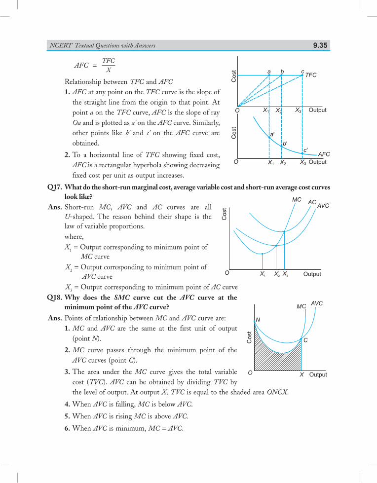
NCERT Textual Questions with Answers 9.35
AFC =TFC
X
Relationship between TFC and AFC1. AFC at any point on the TFC curve is the slope of
the straight line from the origin to that point. At point a on the TFC curve, AFC is the slope of ray Oa and is plotted as a' on the AFC curve. Similarly, other points like b' and c' on the AFC curve are obtained.
2. To a horizontal line of TFC showing fixed cost, AFC is a rectangular hyperbola showing decreasing fixed cost per unit as output increases.
Q17. What do the short-run marginal cost, average variable cost and short-run average cost curves look like?
Ans. Short-run MC, AVC and AC curves are all U-shaped. The reason behind their shape is the law of variable proportions.
where, X1 = Output corresponding to minimum point of
MC curve X2 = Output corresponding to minimum point of
AVC curve X3 = Output corresponding to minimum point of AC curve Q18. Why does the SMC curve cut the AVC curve at the
minimum point of the AVC curve?
Ans. Points of relationship between MC and AVC curve are:1. MC and AVC are the same at the first unit of output
(point N).
2. MC curve passes through the minimum point of the AVC curves (point C).
3. The area under the MC curve gives the total variable cost (TVC). AVC can be obtained by dividing TVC by the level of output. At output X, TVC is equal to the shaded area ONCX.
4. When AVC is falling, MC is below AVC.
5. When AVC is rising MC is above AVC.
6. When AVC is minimum, MC = AVC.
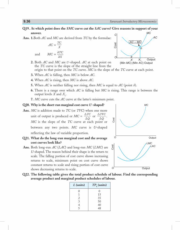
Saraswati Introductory Microeconomics9.36
Q19. At which point does the SMC curve cut the SAC curve? Give reasons in support of your answer.
Ans. 1. Both AC and MC are derived from TC by the formulae:
AC = TCX
and MC = ∂∂TCX
2. Both AC and MC are -shaped. AC at each point on the TC curve is the slope of the straight line from the origin to that point on the TC curve. MC is the slope of the TC curve at each point.
3. When AC is falling, then MC is below AC.4. When AC is rising, then MC is above AC.5. When AC is neither falling nor rising, then MC is equal to AC (point b).6. There is a range over which AC is falling but MC is rising. This range is between the
output levels X and X1.7. MC curve cuts the AC curve at the latter’s minimum point.
Q20. Why is the short-run marginal cost curve U -shaped?
Ans. MC is addition made to TC (or TVC) when one more
unit of output is produced or MC = DD
TCQ
or DDTVC
Q.
MC is the slope of the TC curve at each point or
between any two points. MC curve is U-shaped
reflecting the law of variable proportion. Q21. What do the long-run marginal cost and the average
cost curves look like? Ans. Both long-run AC (LAC) and long-run MC (LMC) are
U-shaped. The reason behind their shape is the return to scale. The falling portion of cost curve shows increasing returns to scale, minimum point on cost curve shows constant returns to scale and rising portion of cost curve shows decreasing returns to scale.
Q22. The following table gives the total product schedule of labour. Find the corresponding average product and marginal product schedules of labour.
L (units) TPL (units)
012345
01535504048
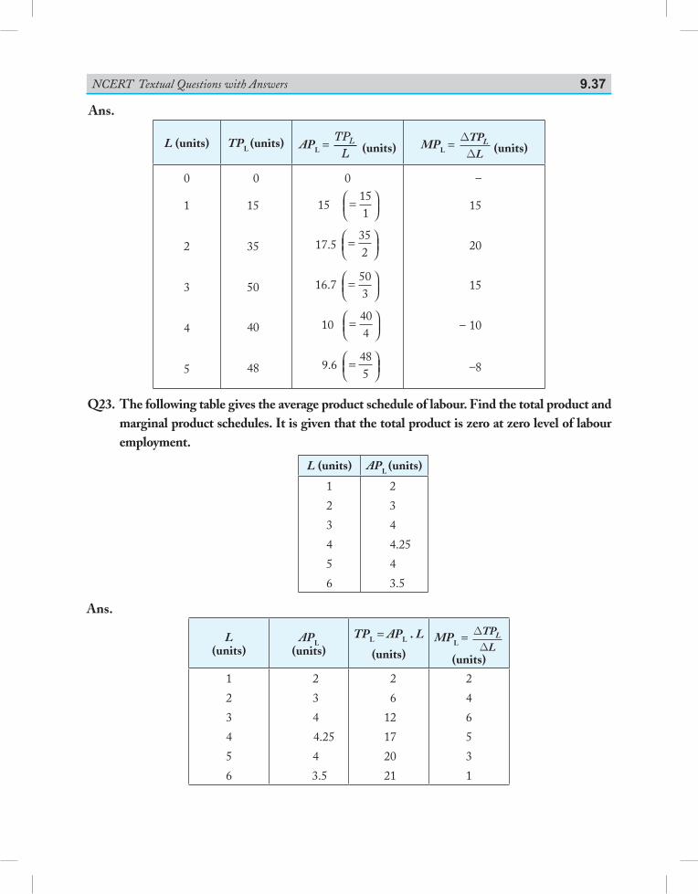
NCERT Textual Questions with Answers 9.37
Ans.
L (units) TPL (units) APL = TPL
L (units) MPL = DDTPLL (units)
0
1
2
3
4
5
0
15
35
50
40
48
0
15 =
151
17.5 =
352
16.7 =
503
10 =
404
9.6 =
485
–
15
20
15
– 10
–8
Q23. The following table gives the average product schedule of labour. Find the total product and marginal product schedules. It is given that the total product is zero at zero level of labour employment.
L (units) APL (units)
1
2
3
4
5
6
2
3
4
4.25
4
3.5
Ans.
L (units)
APL (units)
TPL = APL . L
(units)MPL = D
DTPLL
(units)
1
2
3
4
5
6
2
3
4
4.25
4
3.5
2
6
12
17
20
21
2
4
6
5
3
1
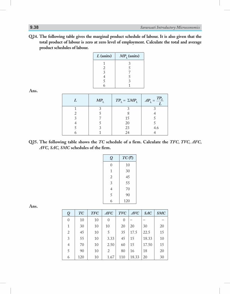
Saraswati Introductory Microeconomics9.38
Q24. The following table gives the marginal product schedule of labour. It is also given that the total product of labour is zero at zero level of employment. Calculate the total and average product schedules of labour.
L (units) MPL (units)
123456
357531
Ans.
L MPL TPL = ΣMPL APL = TPLL
123456
357531
38
15202324
34554.64
Q25. The following table shows the TC schedule of a firm. Calculate the TFC, TVC, AFC, AVC, SAC, SMC schedules of the firm.
Q TC (`)
0123456
103045557090
120 Ans.
Q TC TFC AFC TVC AVC SAC SMC
0
1
2
3
4
5
6
10
30
45
55
70
90
120
10
10
10
10
10
10
10
0
10
5
3.33
2.50
2
1.67
0
20
35
45
60
80
110
–
20
17.5
15
15
16
18.33
–
30
22.5
18.33
17.50
18
20
–
20
15
10
15
20
30
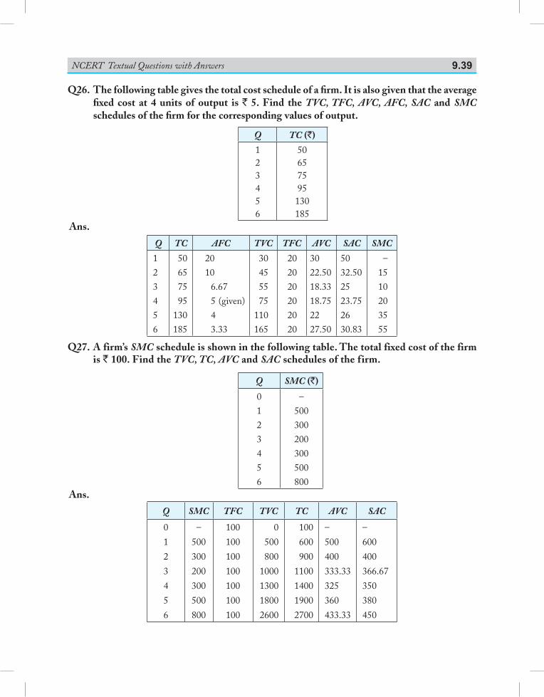
NCERT Textual Questions with Answers 9.39
Q26. The following table gives the total cost schedule of a firm. It is also given that the average fixed cost at 4 units of output is ` 5. Find the TVC, TFC, AVC, AFC, SAC and SMC schedules of the firm for the corresponding values of output.
Q TC (`)
123456
50657595130185
Ans.
Q TC AFC TVC TFC AVC SAC SMC
123456
50657595
130185
2010 6.67 5 (given) 4 3.33
30455575
110165
202020202020
3022.5018.3318.752227.50
5032.502523.752630.83
–1510203555
Q27. A firm’s SMC schedule is shown in the following table. The total fixed cost of the firm is ` 100. Find the TVC, TC, AVC and SAC schedules of the firm.
Q SMC (`)
0123456
–500300200300500800
Ans.
Q SMC TFC TVC TC AVC SAC
0
1
2
3
4
5
6
–
500
300
200
300
500
800
100
100
100
100
100
100
100
0
500
800
1000
1300
1800
2600
100
600
900
1100
1400
1900
2700
–
500
400
333.33
325
360
433.33
–
600
400
366.67
350
380
450
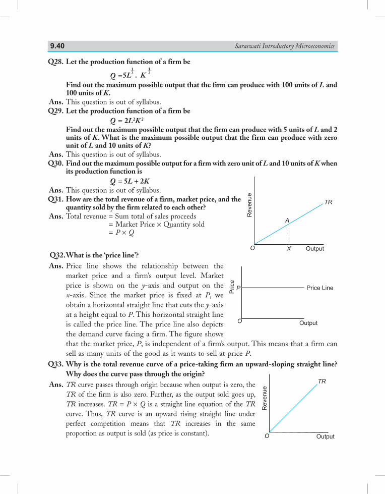
Saraswati Introductory Microeconomics9.40
Q28. Let the production function of a firm be
Q = 5L . K12
12
Find out the maximum possible output that the firm can produce with 100 units of L and 100 units of K.
Ans. This question is out of syllabus. Q29. Let the production function of a firm be Q =2L2K 2
Find out the maximum possible output that the firm can produce with 5 units of L and 2 units of K. What is the maximum possible output that the firm can produce with zero unit of L and 10 units of K?
Ans. This question is out of syllabus. Q30. Find out the maximum possible output for a firm with zero unit of L and 10 units of K when
its production function is Q = 5L + 2K Ans. This question is out of syllabus. Q31. How are the total revenue of a firm, market price, and the
quantity sold by the firm related to each other? Ans. Total revenue =Sum total of sales proceeds = Market Price × Quantity sold = P × Q
Q32. What is the ‘price line’? Ans. Price line shows the relationship between the
market price and a firm’s output level. Market price is shown on the y-axis and output on the x-axis. Since the market price is fixed at P, we obtain a horizontal straight line that cuts the y-axis at a height equal to P. This horizontal straight line is called the price line. The price line also depicts the demand curve facing a firm. The figure shows that the market price, P, is independent of a firm’s output. This means that a firm can sell as many units of the good as it wants to sell at price P.
Q33. Why is the total revenue curve of a price-taking firm an upward-sloping straight line? Why does the curve pass through the origin?
Ans. TR curve passes through origin because when output is zero, the TR of the firm is also zero. Further, as the output sold goes up, TR increases. TR = P × Q is a straight line equation of the TR curve. Thus, TR curve is an upward rising straight line under perfect competition means that TR increases in the same proportion as output is sold (as price is constant).
Revenue
O
TR
Output
Price
O
Price Line
Output
P
Revenue
O X
A
TR
Output
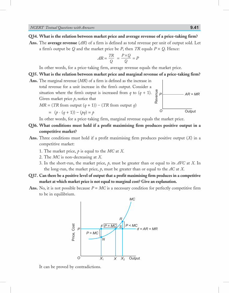
NCERT Textual Questions with Answers 9.41
Q34. What is the relation between market price and average revenue of a price-taking firm? Ans. The average revenue (AR) of a firm is defined as total revenue per unit of output sold. Let
a firm’s output be Q and the market price be P, then TR equals P × Q. Hence:
AR = TRQ
= P Q
Q×
= P
In other words, for a price-taking firm, average revenue equals the market price. Q35. What is the relation between market price and marginal revenue of a price-taking firm? Ans. The marginal revenue (MR) of a firm is defined as the increase in
total revenue for a unit increase in the firm’s output. Consider a situation where the firm’s output is increased from q to (q + 1). Given market price p, notice that
MR = (TR from output (q + 1)) – (TR from output q)
= (p . (q + 1)) – (pq) = p In other words, for a price-taking firm, marginal revenue equals the market price. Q36. What conditions must hold if a profit maximising firm produces positive output in a
competitive market? Ans. Three conditions must hold if a profit maximising firm produces positive output (X) in a
competitive market:
1. The market price, p is equal to the MC at X.2. The MC is non-decreasing at X.3. In the short-run, the market price, p, must be greater than or equal to its AVC at X. In
the long-run, the market price, p, must be greater than or equal to the AC at X. Q37. Can there be a positive level of output that a profit maximising firm produces in a competitive
market at which market price is not equal to marginal cost? Give an explanation. Ans. No, it is not possible because P = MC is a necessary condition for perfectly competitive firm
to be in equilibrium.
Price,C
ost
Output
It can be proved by contradictions.
Revenue
Output
AR = MR
O
P
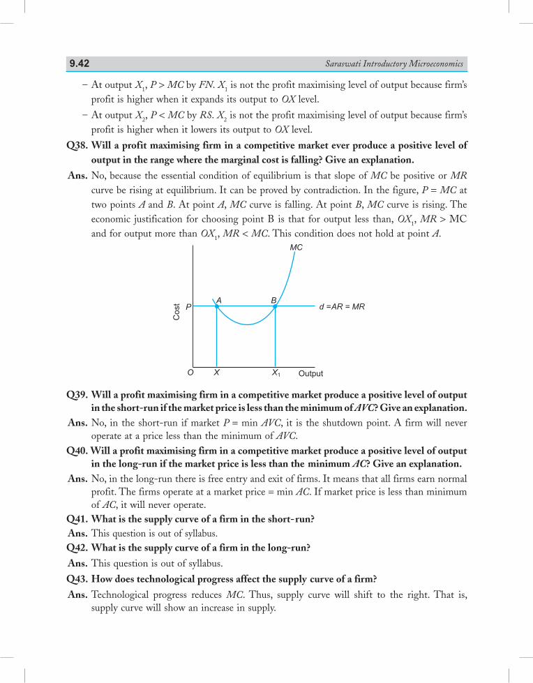
Saraswati Introductory Microeconomics9.42
– At output X1, P > MC by FN. X1 is not the profit maximising level of output because firm’s profit is higher when it expands its output to OX level.
– At output X2, P < MC by RS. X2 is not the profit maximising level of output because firm’s profit is higher when it lowers its output to OX level.
Q38. Will a profit maximising firm in a competitive market ever produce a positive level of output in the range where the marginal cost is falling? Give an explanation.
Ans. No, because the essential condition of equilibrium is that slope of MC be positive or MR curve be rising at equilibrium. It can be proved by contradiction. In the figure, P = MC at two points A and B. At point A, MC curve is falling. At point B, MC curve is rising. The economic justification for choosing point B is that for output less than, OX1, MR > MC and for output more than OX1, MR < MC. This condition does not hold at point A.
Cost
Output
Q39. Will a profit maximising firm in a competitive market produce a positive level of output in the short-run if the market price is less than the minimum of AVC? Give an explanation.
Ans. No, in the short-run if market P = min AVC, it is the shutdown point. A firm will never operate at a price less than the minimum of AVC.
Q40. Will a profit maximising firm in a competitive market produce a positive level of output in the long-run if the market price is less than the minimum AC? Give an explanation.
Ans. No, in the long-run there is free entry and exit of firms. It means that all firms earn normal profit. The firms operate at a market price = min AC. If market price is less than minimum of AC, it will never operate.
Q41. What is the supply curve of a firm in the short- run? Ans. This question is out of syllabus.Q42. What is the supply curve of a firm in the long-run?
Ans. This question is out of syllabus.
Q43. How does technological progress affect the supply curve of a firm?
Ans. Technological progress reduces MC. Thus, supply curve will shift to the right. That is, supply curve will show an increase in supply.
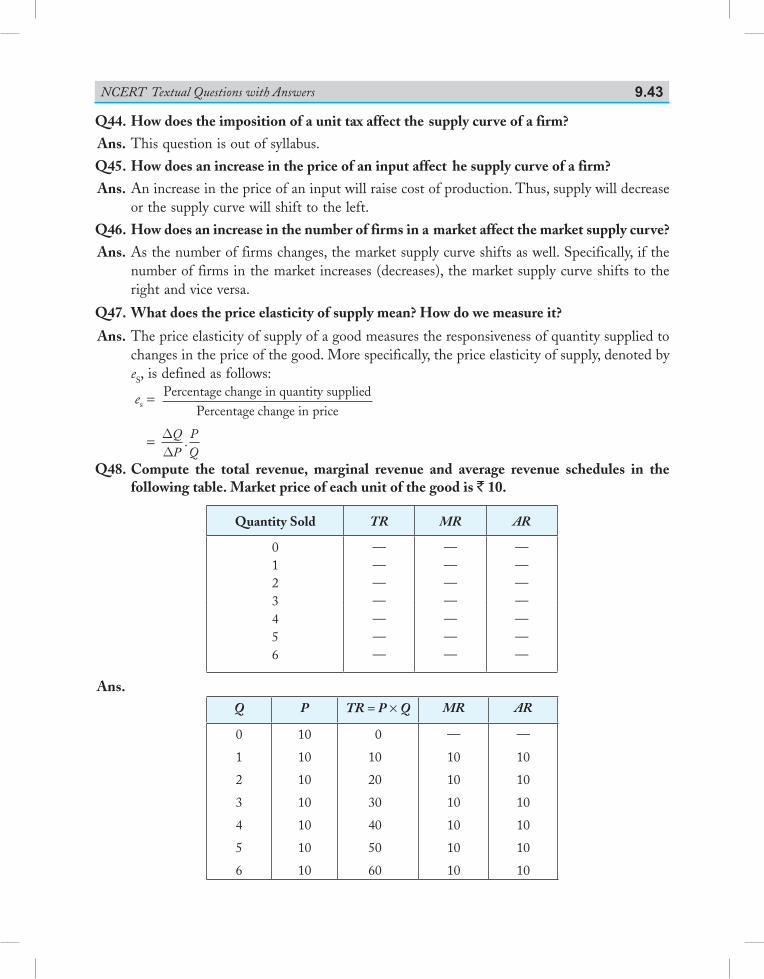
NCERT Textual Questions with Answers 9.43
Q44. How does the imposition of a unit tax affect the supply curve of a firm?
Ans. This question is out of syllabus.
Q45. How does an increase in the price of an input affect he supply curve of a firm?
Ans. An increase in the price of an input will raise cost of production. Thus, supply will decrease or the supply curve will shift to the left.
Q46. How does an increase in the number of firms in a market affect the market supply curve?
Ans. As the number of firms changes, the market supply curve shifts as well. Specifically, if the number of firms in the market increases (decreases), the market supply curve shifts to the right and vice versa.
Q47. What does the price elasticity of supply mean? How do we measure it?
Ans. The price elasticity of supply of a good measures the responsiveness of quantity supplied to changes in the price of the good. More specifically, the price elasticity of supply, denoted by eS, is defined as follows:
es = Percentage change in quantity suppliedPercentage change in price
= DDQP
.PQ
Q48. Compute the total revenue, marginal revenue and average revenue schedules in the following table. Market price of each unit of the good is ` 10.
Quantity Sold TR MR AR
0123
————
————
————
456
———
———
———
Ans.Q P TR = P × Q MR AR
0
1
2
3
4
5
6
10
10
10
10
10
10
10
0
10
20
30
40
50
60
—
10
10
10
10
10
10
—
10
10
10
10
10
10
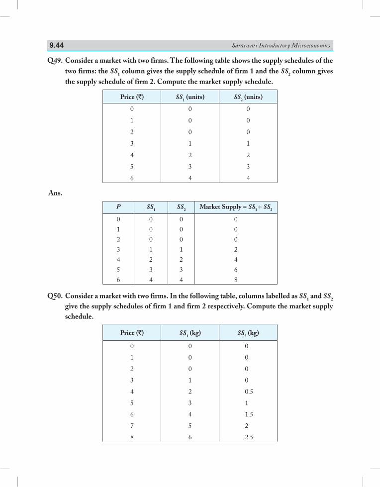
Saraswati Introductory Microeconomics9.44
Q49. Consider a market with two firms. The following table shows the supply schedules of the two firms: the SS1 column gives the supply schedule of firm 1 and the SS2 column gives the supply schedule of firm 2. Compute the market supply schedule.
Price (`) SS1 (units) SS2 (units)
0
1
2
3
4
5
6
0
0
0
1
2
3
4
0
0
0
1
2
3
4
Ans.
P SS1 SS2 Market Supply = SS1 + SS2
0
1
2
3
4
5
6
0
0
0
1
2
3
4
0
0
0
1
2
3
4
0
0
0
2
4
6
8
Q50. Consider a market with two firms. In the following table, columns labelled as SS1 and SS2 give the supply schedules of firm 1 and firm 2 respectively. Compute the market supply schedule.
Price (`) SS1 (kg) SS2 (kg)
0
1
2
3
4
5
6
7
8
0
0
0
1
2
3
4
5
6
0
0
0
0
0.5
1
1.5
2
2.5
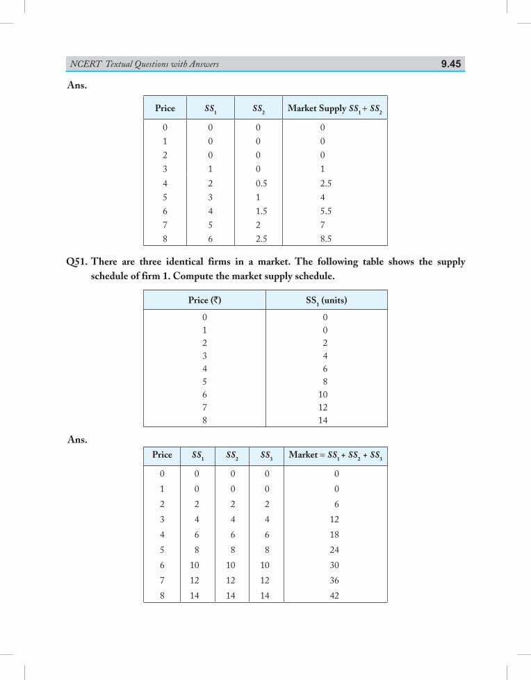
NCERT Textual Questions with Answers 9.45
Ans.
Price SS1 SS2 Market Supply SS1 + SS2
0123
0001
0000
0001
45678
23456
0.511.522.5
2.545.578.5
Q51. There are three identical firms in a market. The following table shows the supply schedule of firm 1. Compute the market supply schedule.
Price (`) SS1 (units)
012345678
002468
101214
Ans.Price SS1 SS2 SS3 Market = SS1 + SS2 + SS3
0
1
2
3
4
5
6
7
8
0
0
2
4
6
8
10
12
14
0
0
2
4
6
8
10
12
14
0
0
2
4
6
8
10
12
14
0
0
6
12
18
24
30
36
42
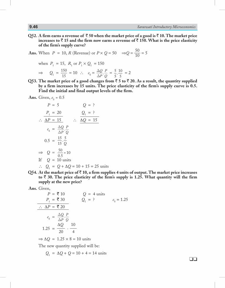
Saraswati Introductory Microeconomics9.46
Q52. A firm earns a revenue of ` 50 when the market price of a good is ` 10. The market price increases to ` 15 and the firm now earns a revenue of ` 150. What is the price elasticity of the firm’s supply curve?
Ans. When P = 10, R (Revenue) or P × Q = 50 ⇒Q = 5010 = 5
when P1 = 15, R1 or P1 × Q1 = 150
⇒ Q1 = 15015
= 10 ∴ eS = DDQPPQ
. = 55
105
. = 2
Q53. The market price of a good changes from ` 5 to ` 20. As a result, the quantity supplied by a firm increases by 15 units. The price elasticity of the firm’s supply curve is 0.5. Find the initial and final output levels of the firm.
Ans. Given, eS = 0.5
P = 5 Q = ?
P1 = 20 Q1 = ?
∴ ΔP = 15 ∴ ΔQ = 15
eS = DD
QP
PQ
.
0.5 = 1515
5.Q
⇒ Q = 500.5
= 10
If Q = 10 units ∴ Q1 = Q + ΔQ = 10 + 15 = 25 units Q54. At the market price of ` 10, a firm supplies 4 units of output. The market price increases
to ` 30. The price elasticity of the firm’s supply is 1.25. What quantity will the firm supply at the new price?
Ans. Given, P = ` 10 Q = 4 units P1 = ` 30 Q1 = ? eS = 1.25
∴ ΔP = ` 20
eS = DD
QP
PQ
.
1.25 = ΔQ
. 10
20 4
⇒ΔQ = 1.25 × 8 = 10 units
The new quantity supplied will be:
Q1 = ΔQ + Q = 10 + 4 = 14 unitsoo

Forms of Marketand
Price Determination Under Perfect Competition with
Simple Applications
UNIT–4
This Unit Contains10. Forms of Market11. Determination of Market Equilibrium
and Effects of Shifts in Demand and Supply Curves
12. Simple Applications of Demand and Supply
10.1 Market—the concept
‘Market’ is a term which is commonly used for a particular place or locality where goods are bought and sold. In economics, market is more than a geographical area or a ‘mandi’ where goods are bought and sold. Market is defined as a complex set of activities by which potential buyers and potential sellers are brought in close contact for the purchase and sale of a commodity. According to Prof. Samuelson, “A market is a mechanism by which buyers and sellers interact to determine the price and quantity of a good or service.” A market can be regional, national or an international market. A market must have the following features:
1. Commodity, i.e., there must be a commodity which is being demanded and sold.2. Buyers and Sellers, i.e., there must be buyers and sellers of the commodity.3. Communication, i.e., there must be communication between buyers and sellers.4. Place or Area, i.e., there must be a place or area where buyers and sellers could interact
with each other.
Chapter Scheme10.1 Market—The Concept10.2 Types of Different Market Structures10.3 Perfect Competition 10.3.1 Meaning of Perfect Competition 10.3.2 Features of Perfect Competition
and their Implications 10.3.3 Comparison Between Pure
Competition and Perfect Competition
10.4 Monopoly 10.4.1 Meaning of Monopoly 10.4.2 Features of Monopoly
10.5 Perfect Competition vs. Monopoly10.6 Monopolistic Competition 10.6.1 Meaning of Monopolistic
Competition 10.6.2 Features of Monopolistic
Competition10.7 Monopolistic Competition vs. Monopoly10.8 Oligopoly 10.8.1 Meaning and Types of Oligopoly 10.8.2 Features of Oligopoly10.9 Comparison of the Four Market Forms Points to Remember Test Your Knowledge Answers to MCQs
10 Forms of Market
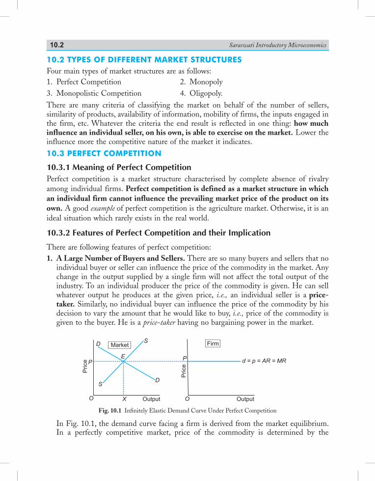
Saraswati Introductory Microeconomics10.2
10.2 types of Different Market structuresFour main types of market structures are as follows:1. Perfect Competition 2. Monopoly3. Monopolistic Competition 4. Oligopoly.There are many criteria of classifying the market on behalf of the number of sellers, similarity of products, availability of information, mobility of firms, the inputs engaged in the firm, etc. Whatever the criteria the end result is reflected in one thing: how much influence an individual seller, on his own, is able to exercise on the market. Lower the influence more the competitive nature of the market it indicates.
10.3 perfect coMpetition
10.3.1 Meaning of Perfect CompetitionPerfect competition is a market structure characterised by complete absence of rivalry among individual firms. Perfect competition is defined as a market structure in which an individual firm cannot influence the prevailing market price of the product on its own. A good example of perfect competition is the agriculture market. Otherwise, it is an ideal situation which rarely exists in the real world.
10.3.2 Features of Perfect Competition and their Implication
There are following features of perfect competition:1. A Large Number of Buyers and Sellers. There are so many buyers and sellers that no
individual buyer or seller can influence the price of the commodity in the market. Any change in the output supplied by a single firm will not affect the total output of the industry. To an individual producer the price of the commodity is given. He can sell whatever output he produces at the given price, i.e., an individual seller is a price-taker. Similarly, no individual buyer can influence the price of the commodity by his decision to vary the amount that he would like to buy, i.e., price of the commodity is given to the buyer. He is a price-taker having no bargaining power in the market.
Fig. 10.1 Infinitely Elastic Demand Curve Under Perfect Competition
In Fig. 10.1, the demand curve facing a firm is derived from the market equilibrium. In a perfectly competitive market, price of the commodity is determined by the
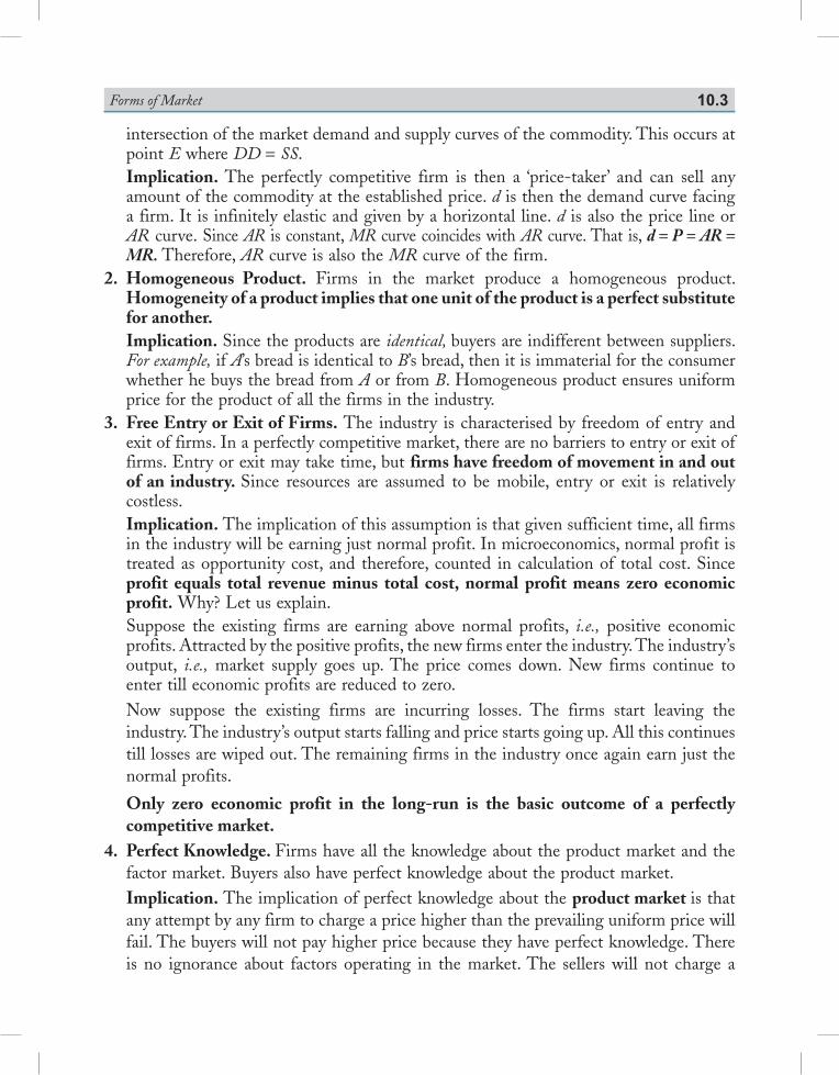
Forms of Market 10.3
intersection of the market demand and supply curves of the commodity. This occurs at point E where DD = SS.
Implication. The perfectly competitive firm is then a ‘price-taker’ and can sell any amount of the commodity at the established price. d is then the demand curve facing a firm. It is infinitely elastic and given by a horizontal line. d is also the price line or AR curve. Since AR is constant, MR curve coincides with AR curve. That is, d = P = AR = MR. Therefore, AR curve is also the MR curve of the firm.
2. Homogeneous Product. Firms in the market produce a homogeneous product. Homogeneity of a product implies that one unit of the product is a perfect substitute for another.
Implication. Since the products are identical, buyers are indifferent between suppliers. For example, if A’s bread is identical to B’s bread, then it is immaterial for the consumer whether he buys the bread from A or from B. Homogeneous product ensures uniform price for the product of all the firms in the industry.
3. Free Entry or Exit of Firms. The industry is characterised by freedom of entry and exit of firms. In a perfectly competitive market, there are no barriers to entry or exit of firms. Entry or exit may take time, but firms have freedom of movement in and out of an industry. Since resources are assumed to be mobile, entry or exit is relatively costless.
Implication. The implication of this assumption is that given sufficient time, all firms in the industry will be earning just normal profit. In microeconomics, normal profit is treated as opportunity cost, and therefore, counted in calculation of total cost. Since profit equals total revenue minus total cost, normal profit means zero economic profit. Why? Let us explain.
Suppose the existing firms are earning above normal profits, i.e., positive economic profits. Attracted by the positive profits, the new firms enter the industry. The industry’s output, i.e., market supply goes up. The price comes down. New firms continue to enter till economic profits are reduced to zero.
Now suppose the existing firms are incurring losses. The firms start leaving the industry. The industry’s output starts falling and price starts going up. All this continues till losses are wiped out. The remaining firms in the industry once again earn just the normal profits.
Only zero economic profit in the long-run is the basic outcome of a perfectly competitive market.
4. Perfect Knowledge. Firms have all the knowledge about the product market and the factor market. Buyers also have perfect knowledge about the product market.
Implication. The implication of perfect knowledge about the product market is that any attempt by any firm to charge a price higher than the prevailing uniform price will fail. The buyers will not pay higher price because they have perfect knowledge. There is no ignorance about factors operating in the market. The sellers will not charge a
Saraswati Introductory Microeconomics10.4
higher price. The buyers will not pay a higher price. Thus, uniform price will prevail in the market.
As regards the knowledge about the input markets, the implicit assumption is that each firm has an equal access to the technology and the inputs used in the technology. No firm has any cost advantage. Cost structure of each firm is the same. All firms have a uniform cost structure.
Since there is uniform price and uniform cost in case of all firms, and since profit equals cost minus price, all the firms earn uniform profits.
5. Perfect Mobility of Factors of Production. The factors of production can move easily from one firm to another. Workers can move between jobs and between places.
Implication. It’s implication is that skills can be learnt easily.
6. Absence of Transportation Cost. All goods are produced locally. Transportation costs are zero.
10.3.3 Comparison Between Pure Competition and Perfect Competition Pure competition is a market situation in which there are a very large number of buyers and sellers, products are homogeneous and there is free entry and exit of firms in the market. Perfect competition is a market situation in which:
(i) There are a very large number of buyers and sellers (ii) Products are homogeneous (iii) Free entry and exit of firms in the market (iv) Perfect knowledge (v) Perfect mobility (vi) Absence of transportation cost. It is a broader concept than pure competition. Pure competition is a part of perfect competition.
10.4 Monopoly
10.4.1 Meaning of Monopoly‘Mono’ means ‘one’ and ‘poly’ means ‘seller’. Monopoly is a market structure in which there is a single firm producing all the output. Example: Government has the monopoly in providing water supply, railways, etc.
10.4.2 Features of MonopolyThe major characteristics of monopoly market structure are:
(a) A Single Firm. The monopolist is the only producer of the good. It is because of some natural conditions or legal restrictions like copyrights, patent law, sole dealership, state monopoly etc. As a result, monopolist has full control over supply of the commodity. That is why a monopolist is called price maker.
Forms of Market 10.5
(b) No Close Substitutes. There are no close substitutes for the commodity. The product sold by monopolist has no close substitute. It may be possible that some substitutes are available but these substitutes are too costly and inconvenient to use. Such substitutes which are easily and quickly used in place of given product are not available in the market. Since a monopolist has no close substitute product, it does not face any competition.
(c) Price Maker with Constraint. The monopolist produces all the output in a particular market. The monopolist is a ‘price-maker’. It does not mean that monopolist can fix both price and the quantity demanded. If he fixes a high price, less commodity will be demanded.
Implication. The result is a downward sloping demand curve as shown in Fig. 10.2. The demand curve is a constraint facing a monopoly firm. Demand curve is also the price line and the AR curve. Since AR is downward sloping, MR lies below AR curve and is twice as steep as the AR curve.
(d) Barriers to Entry. There are significant barriers to entry. That is, entry is blockaded. This barrier may be economic, institutional or artificial in nature. As a result, a monopoly firm earns abnormal profit in the long run.
(e) Price Discrimination. It is one of the most important feature of monopoly. When a monopoly firm charges different prices from different customers for the same product it is called price discrimination. It’s aim is profit maximisation.
10.5 perfect coMpetition vs. Monopoly
Perfect competition and monopoly are extreme situations. Some important points of comparison between the two market forms are:(a) Comparison of Assumptions. A glance at the assumptions of the two forms of market
organisation reveals that monopoly is a direct opposite of perfect competition.
Perfect Competition Monopoly
1. Large number of buyers and sellers2. Products are homogeneous3. Free entry and exit
1. One seller2. No close substitutes3. Barriers to entry
(b) Profit Comparison. In perfect competition, there are no supernormal profits in the long-run but in monopoly supernormal profits are generally earned in the long-run. Thus, profits are higher under monopoly than in perfect competition.
(c) Allocation of Resources. Under perfect competition, there is optimal allocation of resources as P = MC. But since P > MC under monopoly, allocation of the available
Fig. 10.2 Inelastic Demand Curve Under Monopoly
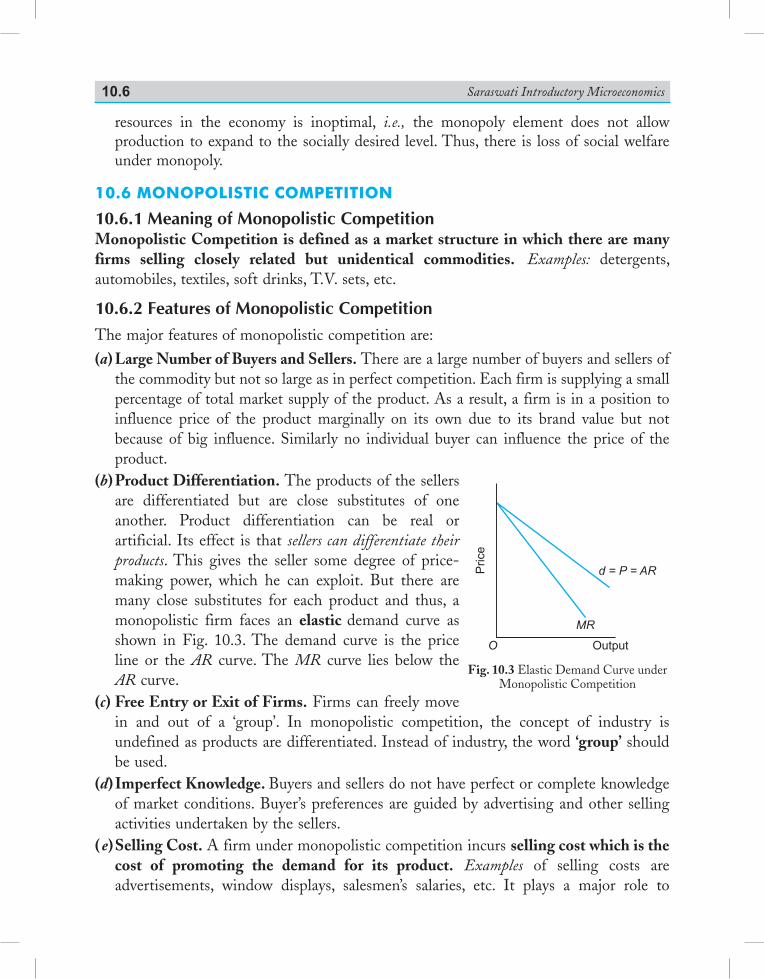
Saraswati Introductory Microeconomics10.6
resources in the economy is inoptimal, i.e., the monopoly element does not allow production to expand to the socially desired level. Thus, there is loss of social welfare under monopoly.
10.6 Monopolistic coMpetition
10.6.1 Meaning of Monopolistic CompetitionMonopolistic Competition is defined as a market structure in which there are many firms selling closely related but unidentical commodities. Examples: detergents, automobiles, textiles, soft drinks, T.V. sets, etc.
10.6.2 Features of Monopolistic CompetitionThe major features of monopolistic competition are:(a) Large Number of Buyers and Sellers. There are a large number of buyers and sellers of
the commodity but not so large as in perfect competition. Each firm is supplying a small percentage of total market supply of the product. As a result, a firm is in a position to influence price of the product marginally on its own due to its brand value but not because of big influence. Similarly no individual buyer can influence the price of the product.
(b) Product Differentiation. The products of the sellers are differentiated but are close substitutes of one another. Product differentiation can be real or artificial. Its effect is that sellers can differentiate their products. This gives the seller some degree of price-making power, which he can exploit. But there are many close substitutes for each product and thus, a monopolistic firm faces an elastic demand curve as shown in Fig. 10.3. The demand curve is the price line or the AR curve. The MR curve lies below the AR curve.
(c) Free Entry or Exit of Firms. Firms can freely move in and out of a ‘group’. In monopolistic competition, the concept of industry is undefined as products are differentiated. Instead of industry, the word ‘group’ should be used.
(d) Imperfect Knowledge. Buyers and sellers do not have perfect or complete knowledge of market conditions. Buyer’s preferences are guided by advertising and other selling activities undertaken by the sellers.
( e) Selling Cost. A firm under monopolistic competition incurs selling cost which is the cost of promoting the demand for its product. Examples of selling costs are advertisements, window displays, salesmen’s salaries, etc. It plays a major role to
Fig. 10.3 Elastic Demand Curve under Monopolistic Competition
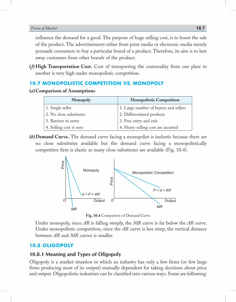
Forms of Market 10.7
influence the demand for a good. The purpose of huge selling cost, is to boost the sale of the product. The advertisements either from print media or electronic media merely persuade consumers to buy a particular brand of a product. Therefore, its aim is to lure away customers from other brands of the product.
( f) High Transportation Cost. Cost of transporting the commodity from one place to another is very high under monopolistic competition.
10.7 Monopolistic coMpetition vs. Monopoly(a) Comparison of Assumptions
Monopoly Monopolistic Competition
1. Single seller
2. No close substitutes
3. Barriers to entry
4. Selling cost is zero
1. Large number of buyers and sellers
2. Differentiated products
3. Free entry and exit
4. Heavy selling cost are incurred
(b) Demand Curve. The demand curve facing a monopolist is inelastic because there are no close substitutes available but the demand curve facing a monopolistically competitive firm is elastic as many close substitutes are available (Fig. 10.4).
Pric
e
Monopoly
d = P = AR
OutputO
MR
Monopolistic Competition
Price
Output
P = d = AR
O
MR
Fig. 10.4 Comparison of Demand Curve
Under monopoly, since AR is falling steeply, the MR curve is far below the AR curve. Under monopolistic competition, since the AR curve is less steep, the vertical distance between AR and MR curves is smaller.
10.8 oliGopoly
10.8.1 Meaning and Types of OligopolyOligopoly is a market situation in which an industry has only a few firms (or few large firms producing most of its output) mutually dependent for taking decisions about price and output. Oligopolistic industries can be classified into various ways. Some are following:
Saraswati Introductory Microeconomics10.8
1. Perfect or Imperfect Oligopoly
If in an oligopoly market, the firms produce homogeneous products, it is called perfect oligopoly. If the firms produce differentiated products, it is called imperfect oligopoly.
2. Non-collusive or Collusive Oligopoly
If in an oligopoly market, the firms compete with each other, it is called a non-collusive, or non-cooperative oligopoly. If the firms cooperate with each other in determining price or output or both, it is called collusive oligopoly, or cooperative oligopoly.
3. Duopoly
When there are only two firms producing a product, it is called duopoly. It is a special case of oligopoly.
10.8.2 Features of Oligopoly
The major features of oligopoly are:
(a) Few Dominant Firms. Oligopolists are often large firms, each producing a significant portion of total market output. There are only a few rival firms. Each big firm has contributed a large proportion into total market supply of the product. Therefore, it can influence the price of the product by its own action and that he can provoke rival firms to react.
(b) Mutual Interdependence. Since the market is dominated by a few firms, the price and output decisions of one firm affects the profitability of the remaining firms in the market. Mutual interdependence is an incentive to develop alternatives to price competition in pursuit of economic profit. Each firm carefully considers and watches how its actions will affect its rivals and how its rivals are likely to react. This makes firms mutually interdependent on each other.
(c) Barriers to Entry. Barriers to entry limits the threat of competition and facilitates the ability of firms to earn long-run economic profits.
(d) Homogeneous or Differentiated Products. The output of an oligopolistic market may be either homogeneous or differentiated.
(e) Demand Curve. In an oligopoly, due to high degree of interdependency amongst oligopolistic firms, that we cannot define the demand curve faced by an oligopolist. Hence, the solution is indeterminate.
Forms of Market 10.9
(f ) Price Rigidity. In oligopolistic firms, prices are administered. Rival firm takes time to react to the changed price, due to which the price remains rigid in this market.
(g) Non-price competition. Firms try to avoid price competition for the fear of price war. They use other methods like advertising, better services to customers, etc. to compete with each other.
10.9 coMparison of the four Market forMs
Table 10.1 Difference between Perfect Competition, Monopolistic Competition, Monopoly and Oligopoly
Reference Perfect Competition
Monopolistic Competition
Monopoly Oligopoly
1. Number of Sellers
Large Large One seller Few sellers
2. Nature of Product
Homogeneous Product differentiation
Homogeneous or differentiated
Homogeneous or differentiated
3. Entry/Exit of Firms
Free entry/exit Free entry/exit Restricted entry/exit
Restricted entry/exit
4. Firm’s Demand Curve
Perfectly elastic Elastic Inelastic Undefined
5. Slope of Firm’s Demand Curve
Horizontal straight line (AR
= MR)
Slopes downward with high elasticity (AR > MR)
Slopes downward with low elasticity (AR > MR)
Depends upon the model
6. Selling Costs Not required Very significant Not required Very significant
7. Degree of Price Control
No control over price or price taker
Limited control over price
Full control over price or price maker
Depends upon themodel
Points to RememberMarket—The Concept
A market is a complex set of activities by which potential buyers and sellers interact to determine the price and quantity of a good or service.
Saraswati Introductory Microeconomics10.10
Types of Market Structures
There are three types of market structures: Perfect competition, monopoly and monopolistic competition.
Perfect Competition
1. It is a market structure in which there are a large number of buyers and sellers selling homogeneous products.
2. Its features are:
Perfect Competition = Pure Competition + Perfect Market Pure competition means: (i) Large number of buyers and sellers (ii) Homogeneous product (iii) Free entry and exit of firms.
Perfect market means: (i) Perfect Knowledge (ii) Perfect mobility of factors of production (iii) Zero transportation cost (iv) Zero selling cost. 3. The demand curve facing the firm is perfectly elastic given by a horizontal line at the
established market price.
Monopoly 1. It is a market structure in which there is only one firm producing the output. 2. Its features are:
(a) A single firm(b) No close substitutes(c) Barriers to entry(d) Perfect knowledge.
3. The demand curve facing the firm is downward sloping and inelastic because the seller is a price-maker. TR curve is inverted U-shaped. MR curve starts from the same point as the AR curve but falls at twice the rate.
Perfect Competition vs MonopolyThe two market situations can be compared on the basis of (a) Assumptions, (b) Profit (c) Allocation of resources (d) Supply curve, and (e) Price and output.
Monopolistic Competition 1. Monopolistic Competition is a market structure in which there are many firms selling closely
related but unidentical commodities. 2. Its features are:
Forms of Market 10.11
(a) Large number of buyers and sellers in the ‘group’(b) The products are differentiated but are close substitutes(c) Free entry and exit(d) Imperfect knowledge(e) Selling cost( f ) High transportation cost.
3. Since the product is somewhat differentiated, the demand curve is downward sloping but its price elasticity is high because competition from close substitutes exist.
Monopolistic Competition vs. MonopolyThe two market forms can be compared on the basis of (a) Assumptions, (b) Demand curve, (c) Profit, (d) Equilibrium conditions, (e) Selling cost.
Oligopoly 1. It is a market structure in which there are few sellers of the commodity. 2. Its features are:
(a) Few dominant firms(b) Mutual interdependence(c) Barriers to entry(d) Price rigidity(e) Non-price competition.
Test Your Knowledge
Very Short Answer Type Questions and MCQs (1 Mark)
1. What is a perfect market? What are its conditions?
2. Under which market form, a firm is a price-taker? (Foreign 2010)
3. Define monopoly. (AI,Foreign 2010)
4. How many firms are there in a monopoly market?
5. In which market form is there product differentiation?
6. In which market form there are restrictions on the entry of new firms?
7. Draw the demand curve of a firm under monopoly.
8. State one characteristic of a perfectly competitive market.
9. Define perfect competition. Give an example.
10. Define monopolistic competition. Give an example.
11. Name the characteristic which makes monopolistic competition different from perfect competition. (Delhi 2010)
Saraswati Introductory Microeconomics10.12
12. State one feature of oligopoly. (Delhi 2010) 13. In which market form demand curve of a firm is perfectly elastic? (Delhi 2010) 14. In which market form can a firm not influence the price of the product? (AI 2010) 15. What can you say about the number of buyers and sellers under monopolistic competition?
(AI 2010) 16. In which market form is a firm a price taker? (Foreign 2010; AI 2013) 17. When is a firm called ‘price-taker’? (Delhi 2011) 18. When is a firm called ‘price-maker’? (AI 2011) 19. What is a price taker firm? (Delhi 2012) 20. What is a price-maker firm? (AI 2012) 21. Define oligopoly. (Foreign 2012) 22. Under which market form a firm’s marginal revenue is always equal to price? (Delhi 2013) 23. What is perfect oligopoly? (Delhi 2014) 24. What is imperfect oligopoly? (AI 2014) 25. What is meant by collusive oligopoly? (Foreign 2014) 26. State any one feature of oligopoly. (Delhi 2017) 27. State any one feature of monopolistic competition. (AI 2017)
Multiple Choice Questions
1. Entry is restricted under: (a) Perfect competition (b) Monopoly (c) Monopolistic competition (d) All of the above
2. Demand curve is perfectly elastic under: (a) Perfect competition (b) Monopoly (c) Monopolistic competition (d) All of the above
3. Demand curve is elastic under: (a) Perfect competition (b) Monopoly (c) Monopolistic competition (d) All of the above
4. Demand curve is inelastic under: (a) Perfect competition (b) Monopoly (c) Monopolistic competition (d) All of the above
5. Differentiated but close substitutes exist under: (a) Perfect competition (b) Monopoly (c) Monopolistic competition (d) All of the above
6. Selling cost is insignificant under: (a) Perfect competition (b) Monopoly (c) Monopolistic competition (d) All of the above
Forms of Market 10.13
7. Few firms exist under: (a) Perfect competition (b) Oligopoly (c) Monopolistic competition (d) Both perfect and monopolistic competition
8. In which market structure, price and output solution is indeterminate? (a) Oligopoly (b) Monopolistic competition (c) Perfect competition (d) Monopoly 9. Homogenous product means products are: (a) Similar (b) Close substitutes (c) Quite alike (d) None of the above
10. Monopoly means: (a) Single firm (b) No close substitutes (c) Barriers to entry (d) All of the above
11. ‘Homogenous products’ is a characteristic of: (Delhi 2016) (a) Perfect competition only (b) Perfect oligopoly only (c) Both (a) and (b) (d) None of the above
12. There is inverse relation between price and demand for the product of a firm under:
(Delhi 2016) (a) Monopoly only (b) Monopolistic competition only (c) Both under monopoly and monopolistic competition (d) Perfect competition only
13. A firm is able to sell any quantity of a good at a given price. The firm’s marginal revenue will be: (AI 2016)
(a) Greater than Average Revenue (b) Less than Average Revenue (c) Equal to Average Revenue (d) Zero
14. Differentiated products is a characteristic of: (AI 2016) (a) Monopolistic competition only (b) Oligopoly only (c) Both monopolistic competition and oligopoly (d) Monopoly
15. Demand curve of a firm is perfectly elastic under: (AI 2016) (a) Perfect competition (b) Monopoly (c) Monopolistic competition (d) Oligopoly
16. Marginal revenue of a firm is constant throughout under: (Foreign 2016) (a) Perfect competition (b) Monopolistic competition (c) Oligopoly (d) All the above
Saraswati Introductory Microeconomics10.14
17. A seller cannot influence the market price under (AI 2017) (a) Perfect Competition (b) Monopoly (c) Monopolistic competition (d) All of the above 18. There are only a few sellers under (Foreign 2017) (a) Perfect Competition (b) Monopolistic competition (c) Monopoly (d) Oligopoly
Short Answer Type Questions (3/4 Marks)
1. What is patent life?
2. State two or three features of perfect competition. 3. Explain the implications of ‘freedom of entry and exit of firms’ under perfect competition.
(Delhi 2010) 4. Why is the number of firms small in an oligopoly market? Explain. (AI 2010) 5. Explain how firms are interdependent in an oligopoly market. (Foreign 2010) 6. Explain the implications of the feature ‘freedom of entry and exit to firms’ under perfect
competition. (Foreign 2011) 7. Explain the implication of ‘perfect knowledge about market’ under perfect competition.
(Delhi 2011) 8. Explain the implication of the feature ‘large number of buyers’ in a perfectly competitive
market. (AI 2011) 9. Explain the implication of large number of buyers in a perfectly competitive market.
(Delhi 2012) 10. Explain the implications of large number of sellers in a perfectly competitive market. (AI 2012) 11. Explain the implications of ‘homogeneous products’ in a perfectly competitive market.
or Explain the implications of ‘differentiated products’ in monopolistic competition. (Foreign 2012) 12. Distinguish between behaviour of average revenue of a firm under monopolistic competition
and perfect competition. Use diagram. (AI 2012) 13. Explain “large number of buyers and sellers” feature of a perfectly competitive market. (Delhi 2013) 14. Explain any two features of monopoly market. (Delhi 2013) 15. Explain “freedom of entry and exit to firms in industry” feature of monopolistic competition. (Delhi 2013) 16. Why can a firm not earn abnormal profits under perfect competition in the long run?
Explain. (AI 2013)
Forms of Market 10.15
17. Giving reasons, state whether the following statement is true or false : (Delhi 2013) A monopolist can sell any quantity he likes at a price. 18. Why are the firms said to be interdependent in an oligopoly market? Explain. (Delhi 2014) 19. Why is the number of firms small in oligopoly? Explain. (AI 2014) 20. There are large number of buyers in a perfectly competitive market. Explain the significance
of this feature. (Delhi 2015) 21. There are no barriers in the way of firms leaving or joining industry in a perfectly competitive
market. Explain the significance of this feature. (Foreign 2015) 22. Explain “perfect knowledge about the markets” feature of perfect competition. (AI 2017) 23. Explain the ‘free entry and exit of firms’ feature of monopolistic competition. (Delhi 2017) 24. Explain the implications of the “freedom of entry and exit” feature of perfect competition.
(Foreign 2017)
Long Answer Type Questions (6 Marks)
1. Distinguish between collusive and non-collusive oligopoly. Explain how the oligopoly firms are interdependent in taking price and output decisions. (Delhi 2011)
2. Distinguish between ‘non-collusive’ and ‘collusive’ oligopoly. Explain the following features of oligopoly:
(i) Few firms (ii) Non-price competition (AI 2011)
3. Distinguish between ‘cooperative’ and ‘non-cooperative’ oligopoly. Explain the following features of oligopoly:
(i) Barriers to the entry of firms
(ii) Non-price competition (Foreign 2011)
4. Giving reasons, state whether the following statements are true or false. (Delhi 2012)
(i) A monopolist can fix both, the price of his product and the quantity to be sold at that price.
(ii) Under monopolistic competition, a firm faces a perfectly elastic demand curve.
5. Give the meaning of ‘collusive’ oligopoly. Explain any two features of oligopoly.
(Foreign 2013)
6. Explain the implications of the following in a perfectly competitive market:
(a) Large number of buyers
(b) Freedom of entry and exit to firms (Delhi 2016)
or
Explain the implications of the following in an oligopoly market:
(a) Inter-dependence between firms
(b) Non-price competition (Delhi 2016)
Saraswati Introductory Microeconomics10.16
7. Explain the implications of the following in an oligopoly market:
(a) Barriers to entry of new firms
(b) A few or a few big sellers (AI 2015, 2016) 8. Distinguish between perfect oligopoly and imperfect oligopoly. Also explain the
“interdependence between the fi rms” feature of oligopoly. (AI 2017)
AnswersMultiple Choice Questions
1. (b) 2. (a) 3. (c) 4. (b) 5. (c) 6. (b) 7. (b) 8. (a) 9. (d) 10. (d) 11. (c) 12. (c) 13. (c) 14. (c ) 15. (a ) 16. (a) 17. (a ) 18. (d)
11.1 Determination of market equilibrium
11.1.1 Meaning of EquilibriumIn economics, the term equilibrium means the state in which there is no tendency on the part of consumers and producers to change. The two factors determining equilibrium price are demand and supply.
Equilibrium Price
Equilibrium price is the price at which the sellers of a good are willing to sell the same quantity which buyers of that good are willing to buy.
Thus, equilibrium price is the price at which demand and supply are equal to each other. At this price, there is no incentive to change.
11.1.2 Market Equilibrium: Fixed Number of FirmsIn the short-run, there are fixed number of firms under perfect competition. Equilibrium price is determined by the equality between demand and supply. At this price,Quantity demanded = Quantity suppliedThe process of determination of equilibrium price has to be studied under three headings:
(a) Demand
(b) Supply
(c) Equilibrium between demand and supply.
11.2.2 Changes in Supply 11.2.3 Simultaneous Changes in both
Demand and Supply Points to Remember Test your Knowledge Answers to MCQs
11.1 Determination of Market Equilibrium 11.1.1 Meaning of Equilibrium 11.1.2 Market Equilibrium: Fixed Number
of Firms11.2 Effects of Changes in Demand and
Supply on Equilibrium Price 11.2.1 Changes in Demand
Chapter Scheme
11Determination of MarketEquilibrium and Effects of Shifts inDemand and Supply Curves
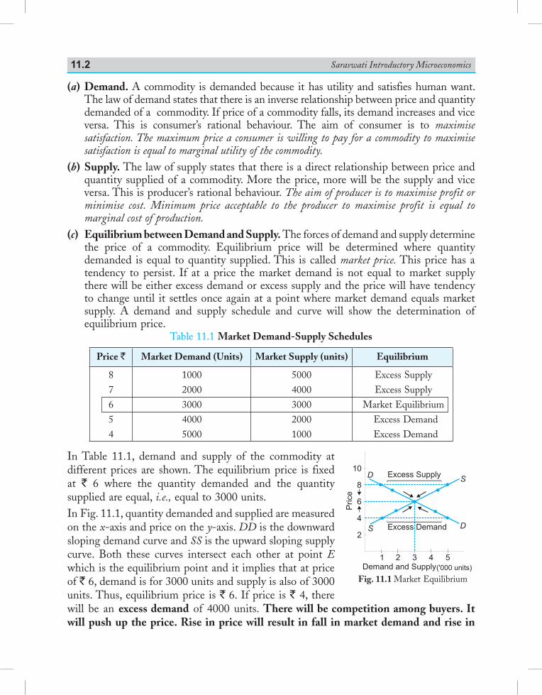
Saraswati Introductory Microeconomics11.2
(a) Demand. A commodity is demanded because it has utility and satisfies human want. The law of demand states that there is an inverse relationship between price and quantity demanded of a commodity. If price of a commodity falls, its demand increases and vice versa. This is consumer’s rational behaviour. The aim of consumer is to maximise satisfaction. The maximum price a consumer is willing to pay for a commodity to maximise satisfaction is equal to marginal utility of the commodity.
(b) Supply. The law of supply states that there is a direct relationship between price and quantity supplied of a commodity. More the price, more will be the supply and vice versa. This is producer’s rational behaviour. The aim of producer is to maximise profit or minimise cost. Minimum price acceptable to the producer to maximise profit is equal to marginal cost of production.
(c) Equilibrium between Demand and Supply. The forces of demand and supply determine the price of a commodity. Equilibrium price will be determined where quantity demanded is equal to quantity supplied. This is called market price. This price has a tendency to persist. If at a price the market demand is not equal to market supply there will be either excess demand or excess supply and the price will have tendency to change until it settles once again at a point where market demand equals market supply. A demand and supply schedule and curve will show the determination of equilibrium price.
Table 11.1 Market Demand-Supply Schedules
Price ` Market Demand (Units) Market Supply (units) Equilibrium
87654
10002000300040005000
50004000300020001000
Excess SupplyExcess Supply
Market EquilibriumExcess DemandExcess Demand
In Table 11.1, demand and supply of the commodity at different prices are shown. The equilibrium price is fixed at ` 6 where the quantity demanded and the quantity supplied are equal, i.e., equal to 3000 units.In Fig. 11.1, quantity demanded and supplied are measured on the x-axis and price on the y-axis. DD is the downward sloping demand curve and SS is the upward sloping supply curve. Both these curves intersect each other at point E which is the equilibrium point and it implies that at price of ` 6, demand is for 3000 units and supply is also of 3000 units. Thus, equilibrium price is ` 6. If price is ` 4, there will be an excess demand of 4000 units. There will be competition among buyers. It will push up the price. Rise in price will result in fall in market demand and rise in
Fig. 11.1 Market Equilibrium
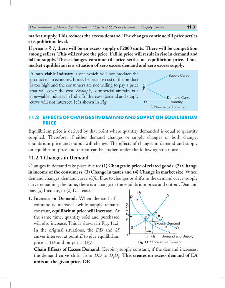
Determination of Market Equilibrium and Effects of Shifts in Demand and Supply Curves 11.3
market supply. This reduces the excess demand. The changes continue till price settles at equilibrium level. If price is ` 7, there will be an excess supply of 2000 units. There will be competition among sellers. This will reduce the price. Fall in price will result in rise in demand and fall in supply. These changes continue till price settles at equilibrium price. Thus, market equilibrium is a situation of zero excess demand and zero excess supply.
A non-viable industry is one which will not produce the product in an economy. It may be because cost of the product is too high and the consumers are not willing to pay a price that will cover the cost. Example, commercial aircrafts is a non-viable industry in India. In this case demand and supply curve will not intersect. It is shown in Fig.
11.2 effects of changes in DemanD anD supply on equilibrium price
Equilibrium price is derived by that point where quantity demanded is equal to quantity supplied. Therefore, if either demand changes or supply changes or both change, equilibrium price and output will change. The effects of changes in demand and supply on equilibrium price and output can be studied under the following situations:
11.2.1 Changes in DemandChanges in demand take place due to: (1) Changes in price of related goods, (2) Change in income of the consumers, (3) Change in tastes and (4) Change in market size. When demand changes, demand curve shifts. Due to changes or shifts in the demand curve, supply curve remaining the same, there is a change in the equilibrium price and output. Demand may (a) Increase, or (b) Decrease.
1. Increase in Demand. When demand of a commodity increases, while supply remains constant, equilibrium price will increase. At the same time, quantity sold and purchased will also increase. This is shown in Fig. 11.2.
In the original situations, the DD and SS curves intersect at point E to give equilibrium price as OP and output as OQ.
Chain Effects of Excess Demand: Keeping supply constant, if the demand increases, the demand curve shifts from DD to D1D1. This creates an excess demand of EA units at the given price, OP.
Supply Curve
Demand Curve
Quantity
Price
OA Non-viable Industry
Fig. 11.2 Increase in Demand
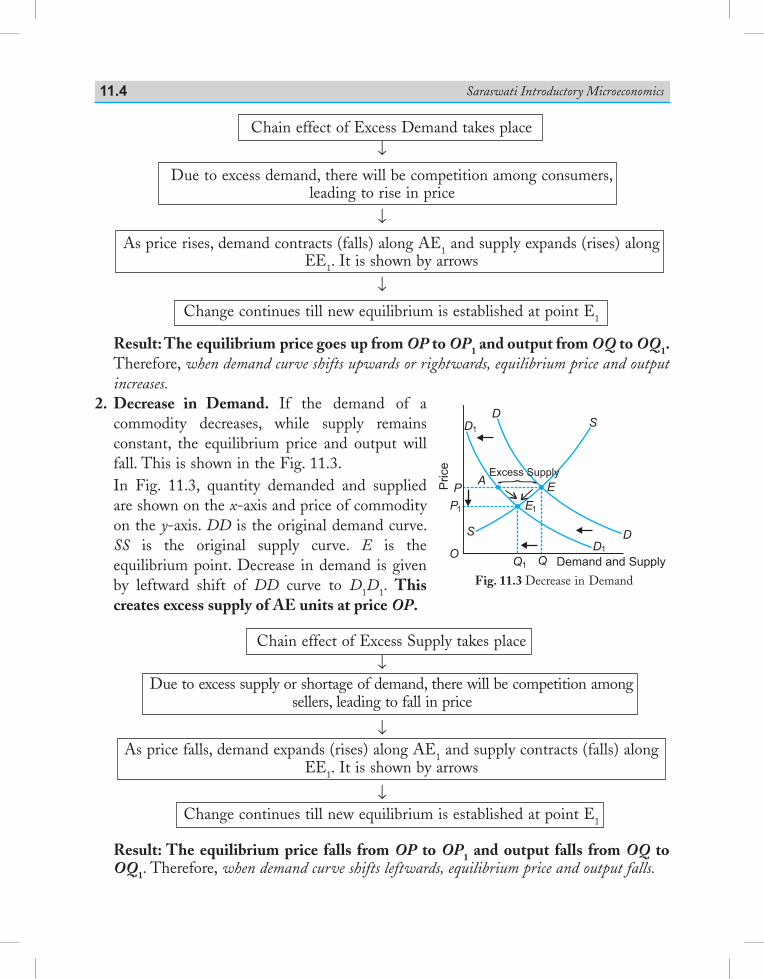
Saraswati Introductory Microeconomics11.4
Chain effect of Excess Demand takes place↓
Due to excess demand, there will be competition among consumers, leading to rise in price
↓ As price rises, demand contracts (falls) along AE1 and supply expands (rises) along
EE1. It is shown by arrows
↓ Change continues till new equilibrium is established at point E1
Result: The equilibrium price goes up from OP to OP1 and output from OQ to OQ1. Therefore, when demand curve shifts upwards or rightwards, equilibrium price and output increases.
2. Decrease in Demand. If the demand of a commodity decreases, while supply remains constant, the equilibrium price and output will fall. This is shown in the Fig. 11.3.
In Fig. 11.3, quantity demanded and supplied are shown on the x-axis and price of commodity on the y-axis. DD is the original demand curve. SS is the original supply curve. E is the equilibrium point. Decrease in demand is given by leftward shift of DD curve to D1D1. This creates excess supply of AE units at price OP.
Chain effect of Excess Supply takes place↓
Due to excess supply or shortage of demand, there will be competition among sellers, leading to fall in price
↓ As price falls, demand expands (rises) along AE1 and supply contracts (falls) along
EE1. It is shown by arrows
↓ Change continues till new equilibrium is established at point E1
Result: The equilibrium price falls from OP to OP1 and output falls from OQ to OQ1. Therefore, when demand curve shifts leftwards, equilibrium price and output falls.
Fig. 11.3 Decrease in Demand
O
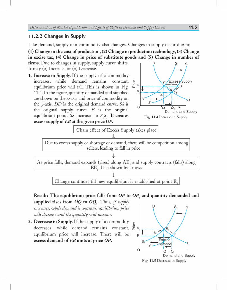
Determination of Market Equilibrium and Effects of Shifts in Demand and Supply Curves 11.5
Price
Demand and Supply
QQ 1
S
P1
S
P
E1
E
D
D S1
S1
O
B
Excess Supply
A
Fig. 11.4 Increase in Supply
11.2.2 Changes in Supply
Like demand, supply of a commodity also changes. Changes in supply occur due to: (1) Change in the cost of production, (2) Change in production technology, (3) Change in excise tax, (4) Change in price of substitute goods and (5) Change in number of firms. Due to changes in supply, supply curve shifts. It may (a) Increase, or (b) Decrease.1. Increase in Supply. If the supply of a commodity
increases, while demand remains constant, equilibrium price will fall. This is shown in Fig. 11.4. In the figure, quantity demanded and supplied are shown on the x-axis and price of commodity on the y-axis. DD is the original demand curve. SS is the original supply curve. E is the original equilibrium point. SS increases to S1S1. It creates excess supply of EB at the given price OP.
Chain effect of Excess Supply takes place↓
Due to excess supply or shortage of demand, there will be competition among sellers, leading to fall in price
↓ As price falls, demand expands (rises) along AE1 and supply contracts (falls) along
EE1. It is shown by arrows
↓ Change continues till new equilibrium is established at point E1
Result: The equilibrium price falls from OP to OP1 and quantity demanded and supplied rises from OQ to OQ1. Thus, if supply increases, while demand is constant, equilibrium price will decrease and the quantity will increase.
2. Decrease in Supply. If the supply of a commodity decreases, while demand remains constant, equilibrium price will increase. There will be excess demand of EB units at price OP.
Fig. 11.5 Decrease in Supply
B
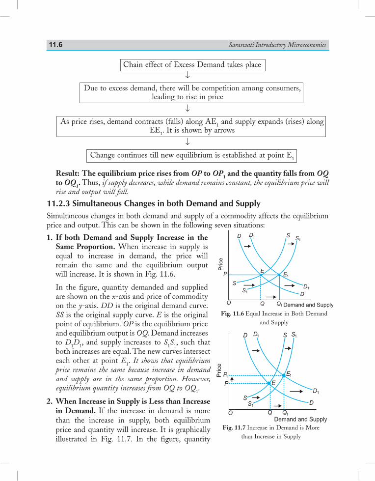
Saraswati Introductory Microeconomics11.6
Chain effect of Excess Demand takes place↓
Due to excess demand, there will be competition among consumers, leading to rise in price
↓ As price rises, demand contracts (falls) along AE1 and supply expands (rises) along
EE1. It is shown by arrows
↓ Change continues till new equilibrium is established at point E1
Result: The equilibrium price rises from OP to OP1 and the quantity falls from OQ to OQ1. Thus, if supply decreases, while demand remains constant, the equilibrium price will rise and output will fall.
11.2.3 Simultaneous Changes in both Demand and SupplySimultaneous changes in both demand and supply of a commodity affects the equilibrium price and output. This can be shown in the following seven situations:
1. If both Demand and Supply Increase in the Same Proportion. When increase in supply is equal to increase in demand, the price will remain the same and the equilibrium output will increase. It is shown in Fig. 11.6.
In the figure, quantity demanded and supplied are shown on the x-axis and price of commodity on the y-axis. DD is the original demand curve. SS is the original supply curve. E is the original point of equilibrium. OP is the equilibrium price and equilibrium output is OQ. Demand increases to D1D1, and supply increases to S1S1, such that both increases are equal. The new curves intersect each other at point E1. It shows that equilibrium price remains the same because increase in demand and supply are in the same proportion. However, equilibrium quantity increases from OQ to OQ1.
2. When Increase in Supply is Less than Increase in Demand. If the increase in demand is more than the increase in supply, both equilibrium price and quantity will increase. It is graphically illustrated in Fig. 11.7. In the figure, quantity
Fig. 11.7 Increase in Demand is More than Increase in Supply
Price
D S
E
S
P
O Q Q1
D1
D
S1D1
P1
S1
E1
Demand and Supply
Price
D1DS1
S
E1
EP
S
S1
D1
D
O Q Q1 Demand and Supply
Fig. 11.6 Equal Increase in Both Demand and Supply
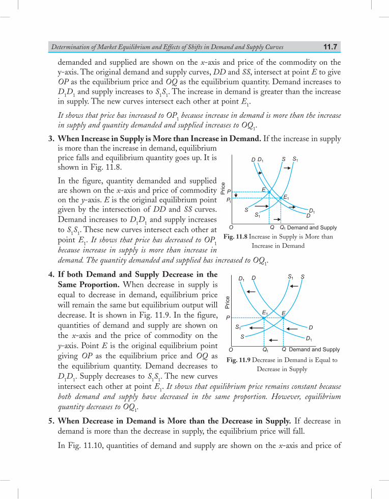
Determination of Market Equilibrium and Effects of Shifts in Demand and Supply Curves 11.7
demanded and supplied are shown on the x-axis and price of the commodity on the y-axis. The original demand and supply curves, DD and SS, intersect at point E to give OP as the equilibrium price and OQ as the equilibrium quantity. Demand increases to D1D1 and supply increases to S1S1. The increase in demand is greater than the increase in supply. The new curves intersect each other at point E1.
It shows that price has increased to OP1 because increase in demand is more than the increase in supply and quantity demanded and supplied increases to OQ1.
3. When Increase in Supply is More than Increase in Demand. If the increase in supply is more than the increase in demand, equilibrium price falls and equilibrium quantity goes up. It is shown in Fig. 11.8.
In the figure, quantity demanded and supplied are shown on the x-axis and price of commodity on the y-axis. E is the original equilibrium point given by the intersection of DD and SS curves. Demand increases to D1D1 and supply increases to S1S1. These new curves intersect each other at point E1. It shows that price has decreased to OP1 because increase in supply is more than increase in demand. The quantity demanded and supplied has increased to OQ1.
4. If both Demand and Supply Decrease in the Same Proportion. When decrease in supply is equal to decrease in demand, equilibrium price will remain the same but equilibrium output will decrease. It is shown in Fig. 11.9. In the figure, quantities of demand and supply are shown on the x-axis and the price of commodity on the y-axis. Point E is the original equilibrium point giving OP as the equilibrium price and OQ as the equilibrium quantity. Demand decreases to D1D1. Supply decreases to S1S1. The new curves intersect each other at point E1. It shows that equilibrium price remains constant because both demand and supply have decreased in the same proportion. However, equilibrium quantity decreases to OQ1.
5. When Decrease in Demand is More than the Decrease in Supply. If decrease in demand is more than the decrease in supply, the equilibrium price will fall.
In Fig. 11.10, quantities of demand and supply are shown on the x-axis and price of
D
Price
D1S1S
SS1
D1
D
E1
EP
P1
Q1QO Demand and Supply
Fig. 11.8 Increase in Supply is More than Increase in Demand
D
Price
D1S1 S
S
S1
D1
D
E1 E
Q1 Q Demand and Supply
P
O
Fig. 11.9 Decrease in Demand is Equal to Decrease in Supply
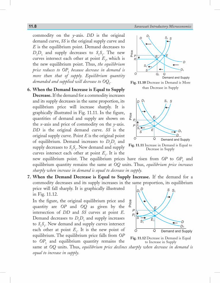
Saraswati Introductory Microeconomics11.8
commodity on the y-axis. DD is the original demand curve, SS is the original supply curve and E is the equilibrium point. Demand decreases to D1D1 and supply decreases to S1S1. The new curves intersect each other at point E1, which is the new equilibrium point. Thus, the equilibrium price reduces to OP1 because decrease in demand is more than that of supply. Equilibrium quantity demanded and supplied will decrease to OQ1.
6. When the Demand Increase is Equal to Supply Decrease. If the demand for a commodity increases and its supply decreases in the same proportion, its equilibrium price will increase sharply. It is graphically illustrated in Fig. 11.11. In the figure, quantities of demand and supply are shown on the x-axis and price of commodity on the y-axis. DD is the original demand curve. SS is the original supply curve. Point E is the original point of equilibrium. Demand increases to D1D1 and supply decreases to S1S1. New demand and supply curves intersect each other at point E1. It is the new equilibrium point. The equilibrium prices have risen from OP to OP1 and equilibrium quantity remains the same at OQ units. Thus, equilibrium price increases sharply when increase in demand is equal to decrease in supply.
7. When the Demand Decrease is Equal to Supply Increase. If the demand for a commodity decreases and its supply increases in the same proportion, its equilibrium price will fall sharply. It is graphically illustrated in Fig. 11.12.
In the figure, the original equilibrium price and quantity are OP and OQ as given by the intersection of DD and SS curves at point E. Demand decreases to D1D1 and supply increases to S1S1. New demand and supply curves intersect each other at point E1. It is the new point of equilibrium. The equilibrium price falls from OP to OP1 and equilibrium quantity remains the same at OQ units. Thus, equilibrium price declines sharply when decrease in demand is equal to increase in supply.
Price
Demand and Supply
P
P1
S1
S S1
S
E
E1
D1
D
DD1
O Q
Fig. 11.12 Decrease in Demand is Equal to Increase in Supply
Demand and Supply
P
O
S
S1
D
D
D1
D1
S1 S
EE1
P
1
Q1 Q
Price
Fig. 11.10 Decrease in Demand is More than Decrease in Supply
Fig. 11.11 Increase in Demand is Equal to Decrease in Supply
Price
Demand and Supply
P
P
1
S1
SS1
SE
E1
D1
D
D D1
O Q
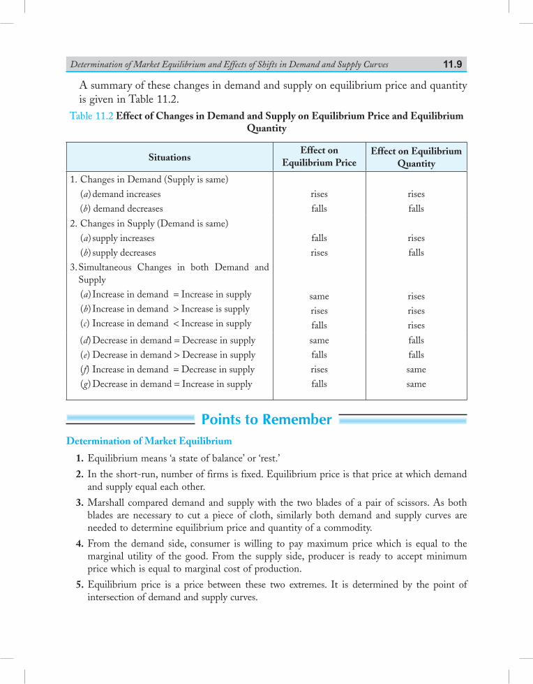
Determination of Market Equilibrium and Effects of Shifts in Demand and Supply Curves 11.9
A summary of these changes in demand and supply on equilibrium price and quantity is given in Table 11.2.
Table 11.2 Effect of Changes in Demand and Supply on Equilibrium Price and Equilibrium Quantity
Situations Effect on
Equilibrium PriceEffect on Equilibrium
Quantity
1. Changes in Demand (Supply is same) (a) demand increases (b) demand decreases
risesfalls
risesfalls
2. Changes in Supply (Demand is same) (a) supply increases (b) supply decreases3. Simultaneous Changes in both Demand and
Supply (a) Increase in demand = Increase in supply (b) Increase in demand > Increase is supply (c) Increase in demand < Increase in supply
fallsrises
samerisesfalls
risesfalls
risesrisesrises
(d) Decrease in demand = Decrease in supply (e) Decrease in demand > Decrease in supply (f) Increase in demand = Decrease in supply (g) Decrease in demand = Increase in supply
samefallsrisesfalls
fallsfallssamesame
Points to RememberDetermination of Market Equilibrium
1. Equilibrium means ‘a state of balance’ or ‘rest.’
2. In the short-run, number of firms is fixed. Equilibrium price is that price at which demand and supply equal each other.
3. Marshall compared demand and supply with the two blades of a pair of scissors. As both blades are necessary to cut a piece of cloth, similarly both demand and supply curves are needed to determine equilibrium price and quantity of a commodity.
4. From the demand side, consumer is willing to pay maximum price which is equal to the marginal utility of the good. From the supply side, producer is ready to accept minimum price which is equal to marginal cost of production.
5. Equilibrium price is a price between these two extremes. It is determined by the point of intersection of demand and supply curves.

Saraswati Introductory Microeconomics11.10
Effects of Changes in Demand and Supply on Equilibrium Price 1. Shifts in demand and supply curves take place due to changes in factors other than the
price of the commodity. 2. A change in demand, supply remaining constant, leads to a change in the equilibrium price.
If demand increases, both equilibrium price and quantity will rise. If demand decreases, both equilibrium price and quantity will fall.
3. A change in supply, demand remaining constant, leads to a change in the equilibrium price and quantity. If supply increases, price will fall and quantity will rise and vice versa if supply decreases.
4. If both demand and supply change, the new equilibrium price may rise, fall or remain constant. For summary, see Table 11.2.
Test Your KnowledgeVery Short Answer Type Questions (1 Mark) 1. When do we say there is excess demand for a commodity in the market?
2. At what price–higher or lower than the equilibrium price, there will be excess demand?
3. When do we say there is excess supply for a commodity in the market?
4. When will an increase in demand imply an increase in price but no change in quantity?
5. When will an increase in demand imply an increase in quantity demanded but no change in price?
6. When will an increase in supply imply an increase in price but no change in quantity?
7. What happens to equilibrium price of a good when the demand for that good increases?
8. At a price of ` 10 per unit of a good, demand for the good is 100 units while supply is 200 units. What is likely to be its effect on price of this good?
9. When will an increase in supply imply an increase in quantity but no change in price?
10. What will happen to equilibrium price, when demand is perfectly elastic and supply increases?
11. What is market equilibrium? (Foreign 2011)
Multiple Choice Questions
1. At a price above the equilibrium price, there is: (a) Excess supply (b) Excess demand (c) Ceiling (d) Flooring
2. At a price below the equilibrium price, there is: (a) Excess supply (b) Excess demand (c) Ceiling (d) Flooring
3. Equilibrium price and output changes when: (a) Demand changes (b) Supply changes (c) Both demand and supply changes (d) All of the above
Determination of Market Equilibrium and Effects of Shifts in Demand and Supply Curves 11.11
4. When demand increases with no change in supply, equilibrium price ...................and quantity ................... .
(a) Rises, rises (b) Rises, falls (c) Falls, falls (d) Falls, rises
5. When demand decreases and there is no shift in supply, the equilibrium price ................... and quantity ................... .
(a) Rises, rises (b) Rises, falls (c) Falls, falls (d) Falls, rises
6. When supply increases and there is no change in demand, then equilibrium price ................... and quantity ................... .
(a) Falls, rises (b) Rises falls (c) Rises rises (d) Falls, falls
7. When supply decreases and there is no change in demand, then equilibrium price ................... and quantity ................... .
(a) Falls, rises (b) Rises, falls (c) Rises, rises (d) Falls, falls
8. When both demand and supply increases in the same proportion then equilibrium price will:
(a) Remain the same (b) Rise (c) Fall (d) None of the above
9. When both demand and supply decreases in the same proportion, then equilibrium price will:
(a) Remain the same (b) Rise (c) Fall (d) None of the above
10. When both demand and supply increase in the same proportion then equilibrium quantity will:
(a) Remain the same (b) Rise (c) Fall (d) None of the above
11. When both demand and supply decrease in the same proportion, then the equilibrium quantity will:
(a) Remain the same (b) Rise (c) Fall (d) None of the above
12. When increase in demand is more than increase in supply, then equilibrium price will:
(a) Remain the same (b) Rise (c) Fall (d) None of the above
Saraswati Introductory Microeconomics11.12
13. When increase in demand in more than increase in supply, then equilibrium quantity will:
(a) Remain the same (b) Rise
(c) Fall (d) None of the above
Short Answer Type Questions (3/4 Marks)
1. Explain the effect of increase in income of buyers of a ‘normal’ commodity on its equilibrium price. (Delhi 2010)
2. How does the equilibrium price of a ‘normal’ commodity change when income of its buyers falls? Explain the chain of effects. (AI 2010)
3. How is the equilibrium price of a commodity affected by a rise in the prices of its substitutes? Explain the chain of effects. (Foreign 2010)
4. How is equilibrium price of a commodity determined under perfect competition? Explain with the help of a numerical example. (Delhi 2012)
5. Explain the chain of effects of excess supply on equilibrium price. (Delhi 2012)
6. Giving reasons, state whether the following statement is true or false. (Delhi 2012)
“Excess supply of a commodity exists when its market price is greater than its equilibrium price”.
7. Equilibrium price of an essential medicine is too high. Explain what possible steps can be taken to bring down the equilibrium price but only through the market forces. Also explain the series of changes that will occur in the market. (AI 2013)
8. Explain the chain effects, if the prevailing market price is below the equilibrium price.
(Delhi 2016)
9. Explain the chain of effects of ‘increase’ in demand of a good. (Foreign 2016)
Long Answer Types Questions (6 Marks)
1. Market for a good is in equilibrium. There is an ‘increase’ in demand for this good. Explain the chain of effects of this change. Use diagram. (Delhi 2011, AI 2014)
2. Market for a good is in equilibrium. There is ‘increase’ in supply of the good. Explain the chain of effects of this change. Use diagram. (AI 2011)
3. Market for a good is in equilibrium. Suppose supply of the good ‘decreases’. Explain the chain of effects of this change. Use diagram. (Foreign 2011, Delhi 2014)
4. Market for a good is in equilibrium. There is simultaneous ‘decrease’ both in demand and supply of the good. Explain its effect on market price. (Delhi 2012)
Determination of Market Equilibrium and Effects of Shifts in Demand and Supply Curves 11.13
5. Market for a good is in equilibrium. Explain the chain of reactions in the market if the price is (i) higher than equilibrium price and (ii) lower than equilibrium price. (AI 2012)
6. Market for a good is in equilibrium. There is simultaneous ‘increase’ both in demand and supply but there is no change in price. Explain how is it possible. Use a schedule.
(Foreign 2012)
7. Explain the changes that take place when market price is greater than equilibrium price. Use diagram. (AI 2012)
8. Giving reasons, state whether the following statement is true or false : (Delhi 2013)
When equilibrium price of a good is less than its market price, there will be competition among the sellers.
9. If equilibrium price of a good is greater than its market price, explain all the changes that will take place in the market. Use diagram. (AI 2013)
10. Explain the effect of “increase” in demand of a good on its equilibrium price and equilibrium quantity. (Foreign 2013)
11. Market for a product is in equilibrium. Demand for the product “decreases”. Explain the chain of effects of this change till the market again reaches equilibrium. Use diagram. (Delhi, AI 2014)
12. Market of a commodity is in equilibrium. Demand for the commodity “increases.” Explain the chain of effects of this change till the market again reaches equilibrium. Use diagram.
(Delhi, AI 2014)
13. What is ‘excess demand’ for a good in a market? Explain its chain of effects on the market for that good. Use diagram. (Foreign 2014)
14. What is meant by ‘excess supply’ of a good in a market? Explain its chain of effects on the market for that good. Use diagram. (Foreign 2014)
15. Market for a good is in equilibrium. The demand for the good ‘increases’. Explain the chain of effects of this change. (Delhi 2015)
16. If the prevailing market price is above the equilibrium price, explain its chain of effects.
(AI 2016)
17. State whether the following statements are true or false. Give reasons for your answer:(Foreign 2017)
(i) When equilibrium price is greater than market price there will be excess supply in the market.
(ii) X and Y are complementary goods. A fall in the price of Y will result in a rise in the price of X.
Saraswati Introductory Microeconomics11.14
18. Explain the meaning of excess demand and excess supply with the help of a schedule. Explain their effect on equilibrium price. (AI 2017)
19. X and Y are substitute goods. The price of Y falls. Explain the chain of effects of this change in the market of X. (Delhi 2017)
or
Explain the chain of effect of excess supply of a good on its equilibirum price.
AnswersMultiple Choice Questions
1. (a) 2. (b) 3. (d) 4. (a) 5. (c) 6. (a) 7. (b) 8. (a) 9. (a) 10. (b) 11. (c) 12. (b) 13. (b)
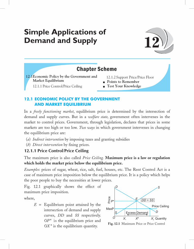
12.1 Economic Policy by thE GovErnmEnt and markEt Equilibrium
In a freely functioning market, equilibrium price is determined by the intersection of demand and supply curves. But in a welfare state, government often intervenes in the market to control prices. Government, through legislation, declares that prices in some markets are too high or too low. Two ways in which government intervenes in changing the equilibrium price are:
(a) Indirect intervention by imposing taxes and granting subsidies (b) Direct intervention by fixing prices.
12.1.1 Price Control/Price Ceiling The maximum price is also called Price Ceiling. Maximum price is a law or regulation which holds the market price below the equilibrium price.
Examples: prices of sugar, wheat, rice, salt, fuel, houses, etc. The Rent Control Act is a case of maximum price imposition below the equilibrium price. It is a policy which helps the poor people to buy the necessities at lower prices.
Fig. 12.1 graphically shows the effect of maximum price imposition.
where,
E = Equilibrium point attained by the intersection of demand and supply curves, DD and SS respectively. OP * i s the equilibrium price and OX * is the equilibrium quantity.
12.1 Economic Policy by the Government and Market Equilibrium
12.1.1 Price Control/Price Ceiling
Chapter Scheme
Simple Applications of Demand and Supply
12.1.2 Support Price/Price Floor Points to Remember Test Your Knowledge
12
Price
Price Ceiling
E
S
D
Quantity
Excess Demand
DD SS=P*
Max.P
O X1
X2
X*
S
D
Fig. 12.1 Maximum Price or Price Control
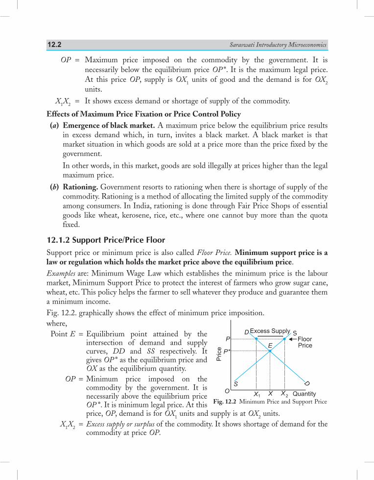
Saraswati Introductory Microeconomics12.2
OP = Maximum price imposed on the commodity by the government. It is necessarily below the equilibrium price OP *. It is the maximum legal price. At this price OP, supply is OX1 units of good and the demand is for OX2 units.
X1X2 = It shows excess demand or shortage of supply of the commodity.
Effects of Maximum Price Fixation or Price Control Policy (a) Emergence of black market. A maximum price below the equilibrium price results
in excess demand which, in turn, invites a black market. A black market is that market situation in which goods are sold at a price more than the price fixed by the government.
In other words, in this market, goods are sold illegally at prices higher than the legal maximum price.
(b) Rationing. Government resorts to rationing when there is shortage of supply of the commodity. Rationing is a method of allocating the limited supply of the commodity among consumers. In India, rationing is done through Fair Price Shops of essential goods like wheat, kerosene, rice, etc., where one cannot buy more than the quota fixed.
12.1.2 Support Price/Price FloorSupport price or minimum price is also called Floor Price. Minimum support price is a law or regulation which holds the market price above the equilibrium price.Examples are: Minimum Wage Law which establishes the minimum price is the labour market, Minimum Support Price to protect the interest of farmers who grow sugar cane, wheat, etc. This policy helps the farmer to sell whatever they produce and guarantee them a minimum income.Fig. 12.2. graphically shows the effect of minimum price imposition.where, Point E = Equilibrium point attained by the
intersection of demand and supply curves, DD and SS respectively. It gives OP * as the equilibrium price and OX as the equilibrium quantity.
OP = Minimum price imposed on the commodity by the government. It is necessarily above the equilibrium price OP *. It is minimum legal price. At this price, OP, demand is for OX1 units and supply is at OX2 units.
X1X2 =Excess supply or surplus of the commodity. It shows shortage of demand for the commodity at price OP.
1 2
Fig. 12.2 Minimum Price and Support Price

Simple Applications of Demand and Supply 12.3
Effects of Minimum Price Fixation or Price Support Policy 1. Farmers or labourers benefit because their income rises. 2. Consumers are worse off as they have to pay higher price (OP) for the good. Otherwise,
they would have paid lower price OP *. 3. It imposes a cost on the government. 4. The government also tries to pass on its burden to the consumers in the form of
higher taxes.
Points to RememberPrice Control/Price Ceiling
1. The maximum price is also called Price Ceiling. Maximum price is a law or regulation which holds the market price below the equilibrium price.
Examples: prices of sugar, wheat, rice, salt, fuel, houses, etc. 2. Effects of price control policy (i) Black Marketing (ii) RationingSupport Price/Price Floor 1. Support price or minimum price is also called Floor Price. Minimum support price is a law
or regulation which holds the market price above the equilibrium price. Examples: Minimum Wage Law 2. Effects of Minimum Price Fixation or Price Support Policy (i) Farmers or labourers benefit because their income rises. (ii) Consumers are worse off as they have to pay higher price (OP) for the good. Otherwise,
they would have paid lower price OP *. (iii) It imposes a cost on the government. (iv) The government also tries to pass on its burden to the consumers in the form of higher taxes.
Test Your KnowledgeVery Short Answer Type Questions (1 Mark) 1. What is price floor? 2. What is price ceiling? 3. What do you mean by black market?Short Answer Type Questions (3/4 Marks) 1. Explain with example the meaning of price ceiling. What are its effects? 2. Explain with example the meaning of price floor. What are its effects? 3. Explain the effects of ‘maximum price ceiling’ on the market of a good. Use diagram. (Delhi 2015) 4. What is price ceiling? Explain the effects of maximum price ceiling. (Delhi 2015) 5. What is maximum price ceiling? Explain its implications. (Delhi 2016) 6. What is minimum price ceiling? Explain its implications. (AI 2016) 7. Explain the meaning of ‘minimum’ price ceiling and its implications. (AI, Foreign 2016)
Long Answer Types Questions (6 Marks) 1. Explain the meaning and implication of maximum price ceiling and minimum price ceiling.
(Foreign 2017)
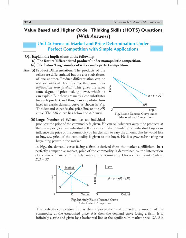
Saraswati Introductory Microeconomics12.4
Value Based and Higher Order Thinking Skills (HOTS) Questions(With Answers)
Unit 4: Forms of Market and Price Determination Under Perfect Competition with Simple Applications
Q1. Explain the implications of the following: (i) The feature ‘differentiated products’ under monopolistic competition. (ii) The feature ‘Large number of sellers’ under perfect competition. Ans. (i) Product Differentiation. The products of the
sellers are differentiated but are close substitutes of one another. Product differentiation can be real or artificial. Its effect is that sellers can differentiate their products. This gives the seller some degree of price-making power, which he can exploit. But there are many close substitutes for each product and thus, a monopolistic firm faces an elastic demand curve as shown in Fig. The demand curve is the price line or the AR curve. The MR curve lies below the AR curve.
(ii) Large Number of Sellers. To an individual producer the price of the commodity is given. He can sell whatever output he produces at the given price, i.e., an individual seller is a price-taker. Similarly, no individual buyer can influence the price of the commodity by his decision to vary the amount that he would like to buy, i.e., price of the commodity is given to the buyer. He is a price-taker having no bargaining power in the market.
In Fig., the demand curve facing a firm is derived from the market equilibrium. In a perfectly competitive market, price of the commodity is determined by the intersection of the market demand and supply curves of the commodity. This occurs at point E where DD = SS.
Fig. Infi nitely Elastic Demand Curve Under Perfect Competition
The perfectly competitive firm is then a ‘price-taker’ and can sell any amount of the commodity at the established price. d is then the demand curve facing a firm. It is infinitely elastic and given by a horizontal line at the equilibrium market price, OP. d is
Pric
e
d P AR= =
O Output
MR
Fig. Elastic Demand Curve underMonopolistic Competition
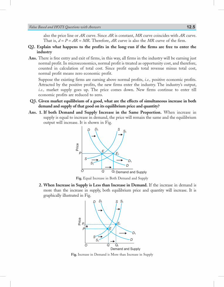
Value Based and HOTS Questions with Answers 12.5
also the price line or AR curve. Since AR is constant, MR curve coincides with AR curve. That is, d = P = AR = MR. Therefore, AR curve is also the MR curve of the firm.
Q2. Explain what happens to the profits in the long-run if the firms are free to enter the industry
Ans. There is free entry and exit of firms, in this way, all firms in the industry will be earning just normal profit. In microeconomics, normal profit is treated as opportunity cost, and therefore, counted in calculation of total cost. Since profit equals total revenue minus total cost, normal profit means zero economic profit.
Suppose the existing firms are earning above normal profits, i.e., positive economic profits. Attracted by the positive profits, the new firms enter the industry. The industry’s output, i.e., market supply goes up. The price comes down. New firms continue to enter till economic profits are reduced to zero.
Q3. Given market equilibrium of a good, what are the effects of simultaneous increase in both demand and supply of that good on its equilibrium price and quantity?
Ans. 1. If both Demand and Supply Increase in the Same Proportion. When increase in supply is equal to increase in demand, the price will remain the same and the equilibrium output will increase. It is shown in Fig.
Price
D1DS1
S
E1
EP
S
S1
D1
D
O Q Q1 Demand and Supply
Fig. Equal Increase in Both Demand and Supply
2. When Increase in Supply is Less than Increase in Demand. If the increase in demand is more than the increase in supply, both equilibrium price and quantity will increase. It is graphically illustrated in Fig.
Price
D S
E
S
P
O Q Q1
D1
D
S1D1
P1
S1
E1
Demand and Supply
Fig. Increase in Demand is More than Increase in Supply
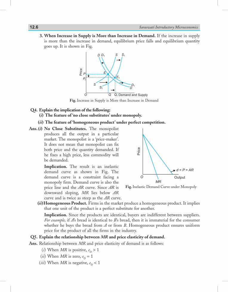
Saraswati Introductory Microeconomics12.6
3. When Increase in Supply is More than Increase in Demand. If the increase in supply is more than the increase in demand, equilibrium price falls and equilibrium quantity goes up. It is shown in Fig.
D
Price
D1S1S
SS1
D1
D
E1
EP
P1
Q1QO Demand and Supply
Fig. Increase in Supply is More than Increase in Demand
Q4. Explain the implication of the following: (i) The feature of ‘no close substitutes’ under monopoly.
(ii) The feature of ‘homogeneous product’ under perfect competition. Ans. (i) No Close Substitutes. The monopolist
produces all the output in a particular market. The monopolist is a ‘price-maker’. It does not mean that monopolist can fix both price and the quantity demanded. If he fixes a high price, less commodity will be demanded.
Implication. The result is an inelastic demand curve as shown in Fig. The demand curve is a constraint facing a monopoly firm. Demand curve is also the price line and the AR curve. Since AR is downward sloping, MR lies below AR curve and is twice as steep as the AR curve.
(ii) Homogeneous Product. Firms in the market produce a homogeneous product. It implies that one unit of the product is a perfect substitute for another.
Implication. Since the products are identical, buyers are indifferent between suppliers. For example, if A’s bread is identical to B’s bread, then it is immaterial for the consumer whether he buys the bread from A or from B. Homogeneous product ensures uniform price for the product of all the firms in the industry.
Q5. Explain the relationship between MR and price elasticity of demand. Ans. Relationship between MR and price elasticity of demand is as follows: (i) When MR is positive, eD > 1 (ii) When MR is zero, eD = 1 (iii) When MR is negative, eD < 1
Fig. Inelastic Demand Curve under Monopoly
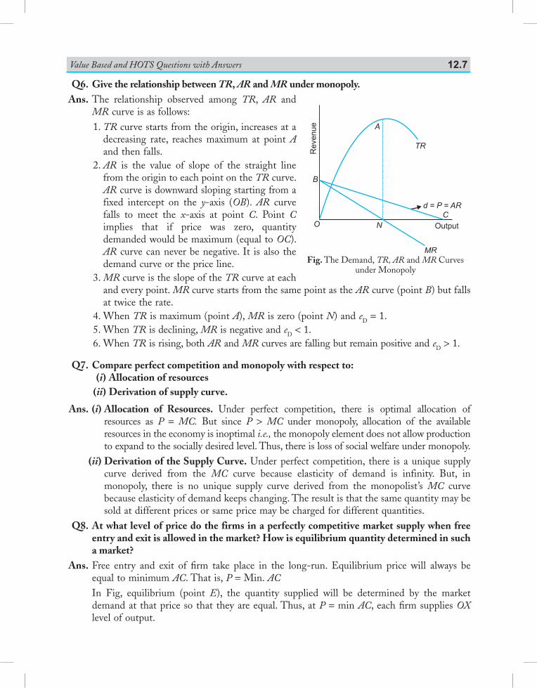
Value Based and HOTS Questions with Answers 12.7
Q6. Give the relationship between TR, AR and MR under monopoly. Ans. The relationship observed among TR, AR and
MR curve is as follows: 1. TR curve starts from the origin, increases at a
decreasing rate, reaches maximum at point A and then falls.
2. AR is the value of slope of the straight line from the origin to each point on the TR curve. AR curve is downward sloping starting from a fixed intercept on the y-axis (OB). AR curve falls to meet the x-axis at point C. Point C implies that if price was zero, quantity demanded would be maximum (equal to OC). AR curve can never be negative. It is also the demand curve or the price line.
3. MR curve is the slope of the TR curve at each and every point. MR curve starts from the same point as the AR curve (point B) but falls at twice the rate.
4. When TR is maximum (point A), MR is zero (point N) and eD = 1. 5. When TR is declining, MR is negative and eD < 1. 6. When TR is rising, both AR and MR curves are falling but remain positive and eD > 1.
Q7. Compare perfect competition and monopoly with respect to: (i) Allocation of resources (ii) Derivation of supply curve.
Ans. (i) Allocation of Resources. Under perfect competition, there is optimal allocation of resources as P = MC. But since P > MC under monopoly, allocation of the available resources in the economy is inoptimal i.e., the monopoly element does not allow production to expand to the socially desired level. Thus, there is loss of social welfare under monopoly.
(ii) Derivation of the Supply Curve. Under perfect competition, there is a unique supply curve derived from the MC curve because elasticity of demand is infinity. But, in monopoly, there is no unique supply curve derived from the monopolist’s MC curve because elasticity of demand keeps changing. The result is that the same quantity may be sold at different prices or same price may be charged for different quantities.
Q8. At what level of price do the firms in a perfectly competitive market supply when free entry and exit is allowed in the market? How is equilibrium quantity determined in such a market?
Ans. Free entry and exit of firm take place in the long-run. Equilibrium price will always be equal to minimum AC. That is, P = Min. AC
In Fig, equilibrium (point E), the quantity supplied will be determined by the market demand at that price so that they are equal. Thus, at P = min AC, each firm supplies OX level of output.
B
O N
MR
Output
C
d = P = AR
TR
A
Re
ve
nu
e
Fig. The Demand, TR, AR and MR Curves under Monopoly
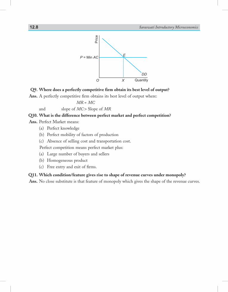
Saraswati Introductory Microeconomics12.8
Quantity
Price
P AC= Min
Q9. Where does a perfectly competitive firm obtain its best level of output? Ans. A perfectly competitive firm obtains its best level of output where: MR = MC and slope of MC > Slope of MRQ10. What is the difference between perfect market and perfect competition? Ans. Perfect Market means: (a) Perfect knowledge (b) Perfect mobility of factors of production (c) Absence of selling cost and transportation cost. Perfect competition means perfect market plus: (a) Large number of buyers and sellers (b) Homogeneous product (c) Free entry and exit of firms.
Q11. Which condition/feature gives rise to shape of revenue curves under monopoly? Ans. No close substitute is that feature of monopoly which gives the shape of the revenue curves.
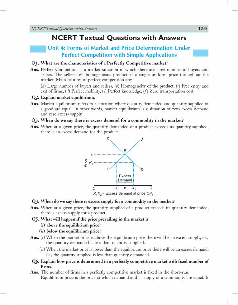
NCERT Textual Questions with Answers 12.9
Q1. What are the characteristics of a Perfectly Competitive market? Ans. Perfect Competiton is a market situation in which there are large number of buyers and
sellers. The sellers sell homogeneous product at a single uniform price throughout the market. Main features of perfect competition are:
(a) Large number of buyers and sellers, (b) Homogeneity of the product, (c) Free entry and exit of firms, (d) Perfect mobility, (e) Perfect knowledge, (f ) Zero transportation cost.
Q2. Explain market equilibrium. Ans. Market equilibrium refers to a situation where quantity demanded and quantity supplied of
a good are equal. In other words, market equilibrium is a situation of zero excess demand and zero excess supply.
Q3. When do we say there is excess demand for a commodity in the market? Ans. When at a given price, the quantity demanded of a product exceeds its quantity supplied,
there is an excess demand for the product.
O
P
Excess
Demand
S
SD
D
P1
X1
X2
X
= Excess demand at price OP1
X1X
2
Q
E
Price
Q4. When do we say there is excess supply for a commodity in the market? Ans. When at a given price, the quantity supplied of a product exceeds its quantity demanded,
there is excess supply for a product. Q5. What will happen if the price prevailing in the market is (i) above the equilibrium price? (ii) below the equilibrium price? Ans. (i) When the market price is above the equilibrium price there will be an excess supply, i.e.,
the quantity demanded is less than quantity supplied. (ii) When the market price is lower than the equilibrium price there will be an excess demand,
i.e., the quantity supplied is less than quantity demanded. Q6. Explain how price is determined in a perfectly competitive market with fixed number of
firms. Ans. The number of firms in a perfectly competitive market is fixed in the short-run. Equilibrium price is the price at which demand and is supply of a commodity are equal. It
NCERT Textual Questions with AnswersUnit 4: Forms of Market and Price Determination Under
Perfect Competition with Simple Applications
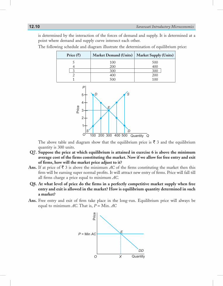
Saraswati Introductory Microeconomics12.10
is determined by the interaction of the forces of demand and supply. It is determined at a point where demand and supply curve intersect each other.
The following schedule and diagram illustrate the determination of equilibrium price:
Price (`) Market Demand (Units) Market Supply (Units)
54321
100200300400500
500400300200100
The above table and diagram show that the equilibrium price is ` 3 and the equilibrium quantity is 300 units.
Q7. Suppose the price at which equilibrium is attained in exercise 6 is above the minimum average cost of the firms constituting the market. Now if we allow for free entry and exit of firms, how will the market price adjust to it?
Ans. If at price of ` 3 is above the minimum AC of the firms constituting the market then this firm will be earning super normal profits. It will attract new entry of firms. Price will fall till all firms charge a price equal to minimum AC.
Q8. At what level of price do the firms in a perfectly competitive market supply when free entry and exit is allowed in the market? How is equilibrium quantity determined in such a market?
Ans. Free entry and exit of firm take place in the long-run. Equilibrium price will always be equal to minimum AC. That is, P = Min. AC
Quantity
Price
P AC= Min
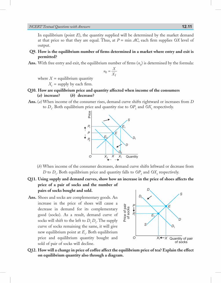
NCERT Textual Questions with Answers 12.11
In equilibrium (point E), the quantity supplied will be determined by the market demand at that price so that they are equal. Thus, at P = min AC, each firm supplies OX level of output.
Q9. How is the equilibrium number of firms determined in a market where entry and exit is permitted?
Ans. With free entry and exit, the equilibrium number of firms (n0) is determined by the formula:
nXX0 =
f where X = equilibrium quantity Xf = supply by each firm. Q10. How are equilibrium price and quantity affected when income of the consumers (a) increase? (b) decrease? Ans. (a) When income of the consumer rises, demand curve shifts rightward or increases from D
to D1. Both equilibrium price and quantity rise to OP1 and OX1 respectively.
Price
Quantity
1
2
2
1
1
2
2 1
(b) When income of the consumer decreases, demand curve shifts leftward or decrease from
D to D1. Both equilibrium price and quantity falls to OP2 and OX2 respectively.
Q11. Using supply and demand curves, show how an increase in the price of shoes affects the price of a pair of socks and the number of pairs of socks bought and sold.
Ans. Shoes and socks are complementary goods. An increase in the price of shoes will cause a decrease in demand for its complementary good (socks). As a result, demand curve of socks will shift to the left to D1 D1. The supply curve of socks remaining the same, it will give new equilibrium point at E1. Both equilibrium price and equilibrium quantity bought and sold of pair of socks will decline.
Q12. How will a change in price of coffee affect the equilibrium price of tea? Explain the effect on equilibrium quantity also through a diagram.
Price
ofpair
ofsocks
Quantity of pair
of socks
11
1
1
1
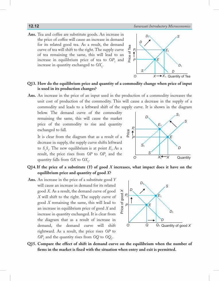
Saraswati Introductory Microeconomics12.12
Ans. Tea and coffee are substitute goods. An increase in the price of coffee will cause an increase in demand for its related good tea. As a result, the demand curve of tea will shift to the right. The supply curve of tea remaining the same, this will lead to an increase in equilibrium price of tea to OP1 and increase in quantity exchanged to OX1.
Q13. How do the equilibrium price and quantity of a commodity change when price of input is used in its production changes?
Ans. An increase in the price of an input used in the production of a commodity increases the unit cost of production of the commodity. This will cause a decrease in the supply of a commodity and leads to a leftward shift of the supply curve. It is shown in the diagram below. The demand curve of the commodity remaining the same, this will cause the market price of the commodity to rise and quantity exchanged to fall.
It is clear from the diagram that as a result of a decrease in supply, the supply curve shifts leftward to S1S1. The new equilibrium is at point E1. As a result, the price rises from OP to OP1 and the quantity falls from OX to OX1.
Q14. If the price of a substitute (Y) of good X increases, what impact does it have on the equilibrium price and quantity of good X?
Ans. An increase in the price of a substitute good Y will cause an increase in demand for its related good X. As a result, the demand curve of good X will shift to the right. The supply curve of good X remaining the same, this will lead to an increase in equilibrium price of good X and increase in quantity exchanged. It is clear from the diagram that as a result of increase in demand, the demand curve will shift rightward. As a result, the price rises OP to OP1 and the quantity rises from OQ to OQ1.
Q15. Compare the effect of shift in demand curve on the equilibrium when the number of firms in the market is fixed with the situation when entry and exit is permitted.
X1XO
P
S
S
E1
E
D1
D1
P1
D
D
Quantity of Tea
Price
ofTea
Price
Quantity
1
1
1
1
1
X X
Pric
e of
goo
dX
Quantity of good X
1
1
1
1
1
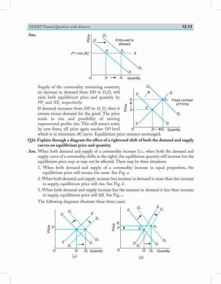
NCERT Textual Questions with Answers 12.13
Ans.
Supply of the commodity remaining constant, an increase in demand from DD to D1D1 will raise both equilibrium price and quantity by PP1 and XX1 respectively.
If demand increases from DD to D1 D1 then it creates excess demand for the good. The price tends to rise and possibility of earning supernormal profits rise. This will attract entry by new firms, till price again reaches OP level which is at minimum AC curve. Equilibrium price remains unchanged.
Q16. Explain through a diagram the effect of a rightward shift of both the demand and supply curves on equilibrium price and quantity.
Ans. When both demand and supply of a commodity increase (i.e., when both the demand and supply curve of a commodity shifts to the right), the equilibrium quantity will increase but the equilibrium price may or may not be affected. There may be three situations:
1. When both demand and supply of a commodity increase in equal proportion, the equilibrium price will remain the same. See Fig. a.
2. When both demand and supply increase but increase in demand is more than the increase in supply, equilibrium price will rise. See Fig. b.
3. When both demand and supply increase but the increase in demand is less than increase in supply, equilibrium price will fall. See Fig. c.
The following diagrams illustrate these three cases:
Quantity
Price
11
1
1
1
1
1
(b)
Quantity
Price
1
1
1
1
1
(a)
P AC= min S
Quantity
Pric
e 1
1
1
1
Entry-exit isallowed
Quantity
Price
1
1
1
1
1
Fixed number
of Firms
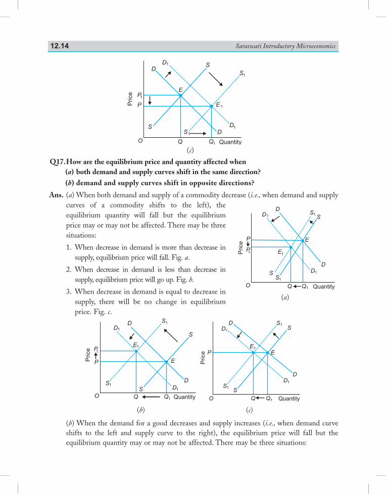
Saraswati Introductory Microeconomics12.14
Quantity
Price
1
1
1
1
1
1
1
(c)
Q17. How are the equilibrium price and quantity affected when(a) both demand and supply curves shift in the same direction?(b) demand and supply curves shift in opposite directions?
Ans. (a) When both demand and supply of a commodity decrease (i.e., when demand and supply curves of a commodity shifts to the left), the equilibrium quantity will fall but the equilibrium price may or may not be affected. There may be three situations:
1. When decrease in demand is more than decrease in supply, equilibrium price will fall. Fig. a.
2. When decrease in demand is less than decrease in supply, equilibrium price will go up. Fig. b.
3. When decrease in demand is equal to decrease in supply, there will be no change in equilibrium price. Fig. c.
Price
Quantity
1
1
1
1
1
1
1
(b) (c)
Q1QO Quantity
Price
E1
E
D1
D1
S1
S1
D
P
S
S
D
(b) When the demand for a good decreases and supply increases (i.e., when demand curve shifts to the left and supply curve to the right), the equilibrium price will fall but the equilibrium quantity may or may not be affected. There may be three situations:
Quantity
Price
11
1
1
1
11
(a)
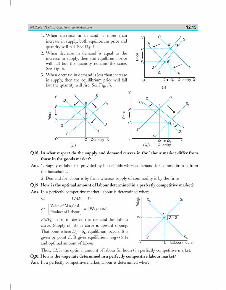
NCERT Textual Questions with Answers 12.15
1. When decrease in demand is more than increase in supply, both equilibrium price and quantity will fall. See Fig. i.
2. When decrease in demand is equal to the increase in supply, then the equilbrium price will fall but the quantity remains the same. See Fig. ii.
3. When decrease in demand is less than increase in supply, then the equilibrium price will fall but the quantity will rise. See Fig. iii.
Q18. In what respect do the supply and demand curves in the labour market differ from those in the goods market?
Ans. 1. Supply of labour is provided by households whereas demand for commodities is from the households.
2. Demand for labour is by firms whereas supply of commodity is by the firms.
Q19. How is the optimal amount of labour determined in a perfectly competitive market?
Ans. In a perfectly competitive market, labour is determined where, or VMPL = W
or Value of MarginalProduct of Labour
[Wage rate]
=
VMPL helps to derive the demand for labour curve. Supply of labour curve is upward sloping. That point where DL = SL, equilibrium occurs. It is given by point E. It gives equilibrium wag++6`1e and optimal amount of labour.
Thus, OL is the optimal amount of labour (in hours) in perfectly competitive market. Q20. How is the wage rate determined in a perfectly competitive labour market? Ans. In a perfectly competitive market, labour is determined where,
(iii)(ii)
Q1
P1
XQO Quantity
Pric
e
D1
D1
S1
S1
P
Y
S
S
E
D
D
E
1
(i)
P1
XQ Q1O
Quantity
Price
D1
D1
1
S1
S1
P
Y
S
S
E
D
D
EP1
XQO Quantity
Pric
e
D1
D1
S1
S1P
Y
S
S
E
D
D
E1
S
L
D
E
O Labour (hours)
Wag
e
SD =
S
DL
W
L
LL
L L
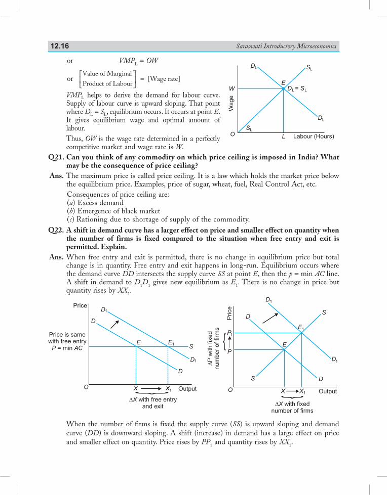
Saraswati Introductory Microeconomics12.16
or VMPL = OW
or Value of MarginalProduct of Labour
[Wage rate]
=
VMPL helps to derive the demand for labour curve. Supply of labour curve is upward sloping. That point where DL = SL, equilibrium occurs. It occurs at point E. It gives equilibrium wage and optimal amount of labour.
Thus, OW is the wage rate determined in a perfectly competitive market and wage rate is W.
Q21. Can you think of any commodity on which price ceiling is imposed in India? What may be the consequence of price ceiling?
Ans. The maximum price is called price ceiling. It is a law which holds the market price below the equilibrium price. Examples, price of sugar, wheat, fuel, Real Control Act, etc.
Consequences of price ceiling are: (a) Excess demand (b) Emergence of black market (c) Rationing due to shortage of supply of the commodity. Q22. A shift in demand curve has a larger effect on price and smaller effect on quantity when
the number of firms is fixed compared to the situation when free entry and exit is permitted. Explain.
Ans. When free entry and exit is permitted, there is no change in equilibrium price but total change is in quantity. Free entry and exit happens in long-run. Equilibrium occurs where the demand curve DD intersects the supply curve SS at point E, then the p = min AC line. A shift in demand to D1D1 gives new equilibrium as E1. There is no change in price but quantity rises by XX1.
∆X with fixednumber of firms
∆Pw
ith
fixed
num
ber
offirm
s
Price
Output1
1
1
1
1
When the number of firms is fixed the supply curve (SS) is upward sloping and demand curve (DD) is downward sloping. A shift (increase) in demand has a large effect on price and smaller effect on quantity. Price rises by PP1 and quantity rises by XX1.
Labour (Hours)
Wa
ge
E
DL
W
SL
D SL L=
SL
DL
L
Price is samewith free entry
= minP ACE
D
D
XO
D
E
X
∆X with free entryand exit
Output
Price
1
1
1
D1
S
O
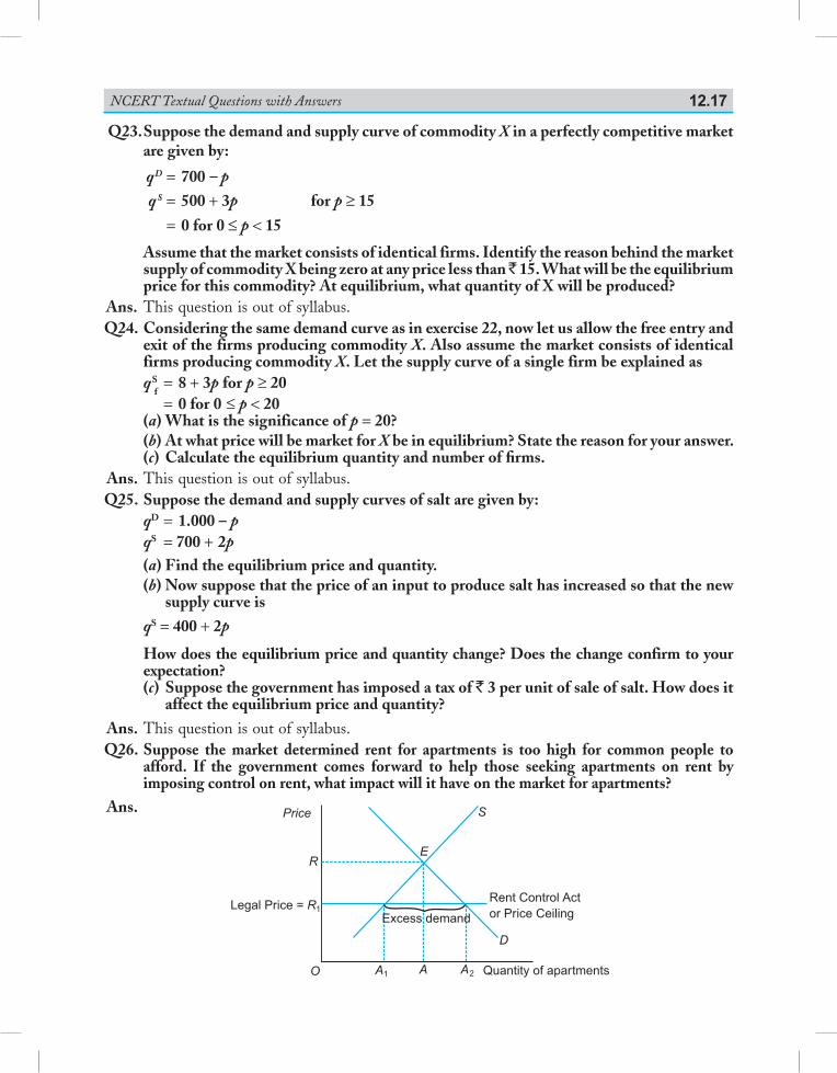
NCERT Textual Questions with Answers 12.17
Q23. Suppose the demand and supply curve of commodity X in a perfectly competitive market are given by:
qD = 700 – p
q S = 500 + 3p for p ≥ 15
= 0 for 0 ≤ p < 15
Assume that the market consists of identical firms. Identify the reason behind the market supply of commodity X being zero at any price less than ̀ 15. What will be the equilibrium price for this commodity? At equilibrium, what quantity of X will be produced?
Ans. This question is out of syllabus.Q24. Considering the same demand curve as in exercise 22, now let us allow the free entry and
exit of the firms producing commodity X. Also assume the market consists of identical firms producing commodity X. Let the supply curve of a single firm be explained as
qSf = 8 + 3p for p ≥ 20
= 0 for 0 ≤ p < 20(a) What is the significance of p = 20?(b) At what price will be market for X be in equilibrium? State the reason for your answer.(c) Calculate the equilibrium quantity and number of firms.
Ans. This question is out of syllabus. Q25. Suppose the demand and supply curves of salt are given by: qD = 1.000 – p qS = 700 + 2p
(a) Find the equilibrium price and quantity.(b) Now suppose that the price of an input to produce salt has increased so that the new
supply curve is qS = 400 + 2p
How does the equilibrium price and quantity change? Does the change confirm to your expectation?(c) Suppose the government has imposed a tax of ` 3 per unit of sale of salt. How does it
affect the equilibrium price and quantity? Ans. This question is out of syllabus. Q26. Suppose the market determined rent for apartments is too high for common people to
afford. If the government comes forward to help those seeking apartments on rent by imposing control on rent, what impact will it have on the market for apartments?
Ans.
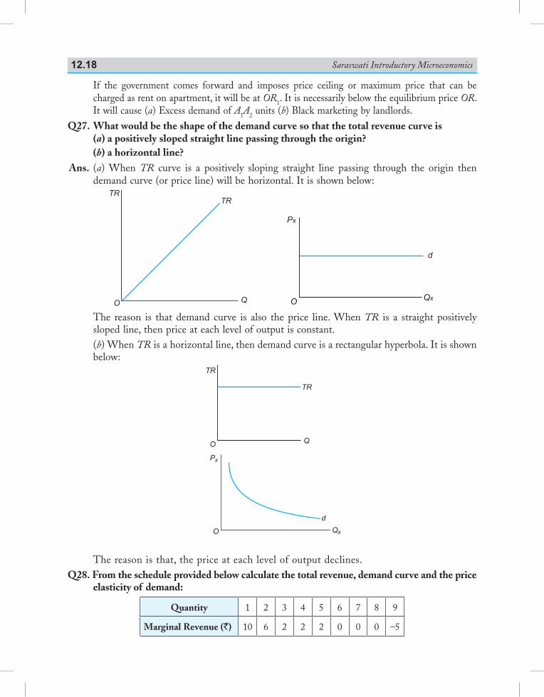
Saraswati Introductory Microeconomics12.18
If the government comes forward and imposes price ceiling or maximum price that can be charged as rent on apartment, it will be at OR1. It is necessarily below the equilibrium price OR. It will cause (a) Excess demand of A1A2 units (b) Black marketing by landlords.
Q27. What would be the shape of the demand curve so that the total revenue curve is (a) a positively sloped straight line passing through the origin?(b) a horizontal line?
Ans. (a) When TR curve is a positively sloping straight line passing through the origin then demand curve (or price line) will be horizontal. It is shown below:
The reason is that demand curve is also the price line. When TR is a straight positively
sloped line, then price at each level of output is constant. (b) When TR is a horizontal line, then demand curve is a rectangular hyperbola. It is shown
below:
The reason is that, the price at each level of output declines. Q28. From the schedule provided below calculate the total revenue, demand curve and the price
elasticity of demand:
Quantity 1 2 3 4 5 6 7 8 9
Marginal Revenue (`) 10 6 2 2 2 0 0 0 –5
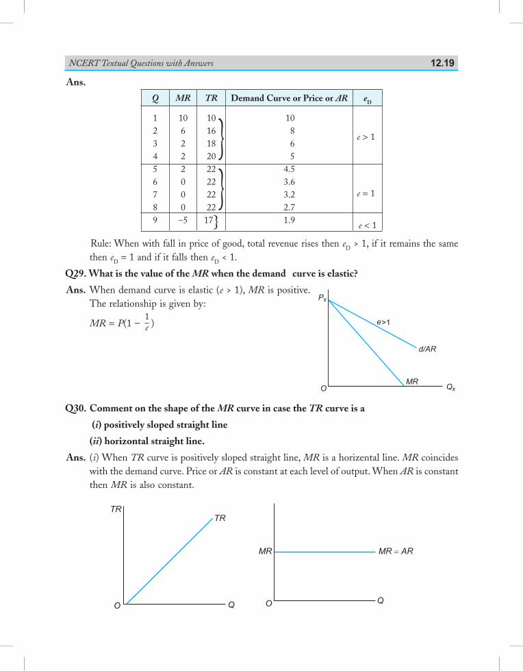
NCERT Textual Questions with Answers 12.19
Ans.
Q MR TR Demand Curve or Price or AR eD
123456789
106222000–5
1016182022222222
17}
10865
4.53.63.22.71.9
e > 1
e = 1
e < 1
Rule: When with fall in price of good, total revenue rises then eD > 1, if it remains the same then eD = 1 and if it falls then eD < 1.
Q29. What is the value of the MR when the demand curve is elastic?
Ans. When demand curve is elastic (e > 1), MR is positive. The relationship is given by:
MR = P(1 – 1e )
Q30. Comment on the shape of the MR curve in case the TR curve is a
(i) positively sloped straight line
(ii) horizontal straight line.
Ans. (i) When TR curve is positively sloped straight line, MR is a horizental line. MR coincides with the demand curve. Price or AR is constant at each level of output. When AR is constant then MR is also constant.
TR
QO
TR
QO
MR MR AR�
}}
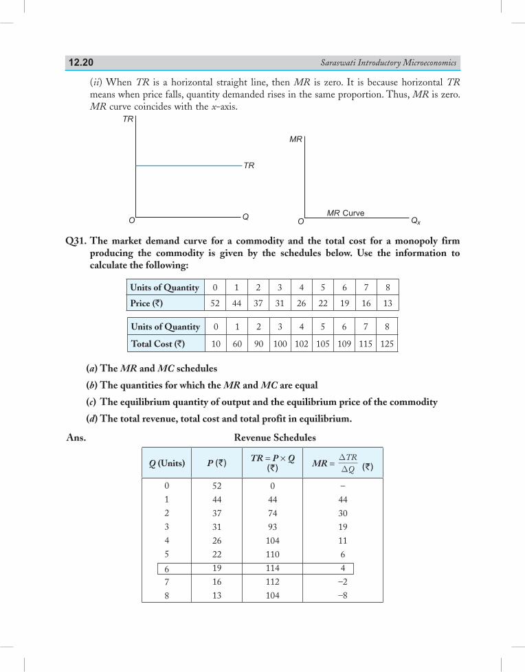
Saraswati Introductory Microeconomics12.20
(ii) When TR is a horizontal straight line, then MR is zero. It is because horizontal TR means when price falls, quantity demanded rises in the same proportion. Thus, MR is zero. MR curve coincides with the x-axis.
Q31. The market demand curve for a commodity and the total cost for a monopoly firm producing the commodity is given by the schedules below. Use the information to calculate the following:
Units of Quantity 0 1 2 3 4 5 6 7 8
Price (`) 52 44 37 31 26 22 19 16 13
Units of Quantity 0 1 2 3 4 5 6 7 8
Total Cost (`) 10 60 90 100 102 105 109 115 125
(a) The MR and MC schedules
(b) The quantities for which the MR and MC are equal
(c) The equilibrium quantity of output and the equilibrium price of the commodity
(d) The total revenue, total cost and total profit in equilibrium.
Ans. Revenue Schedules
Q (Units) P (`) TR = P × Q (`) MR =
DD
TRQ
(`)
012345
6 78
524437312622191613
0447493104110114112104
–4430191164–2–8
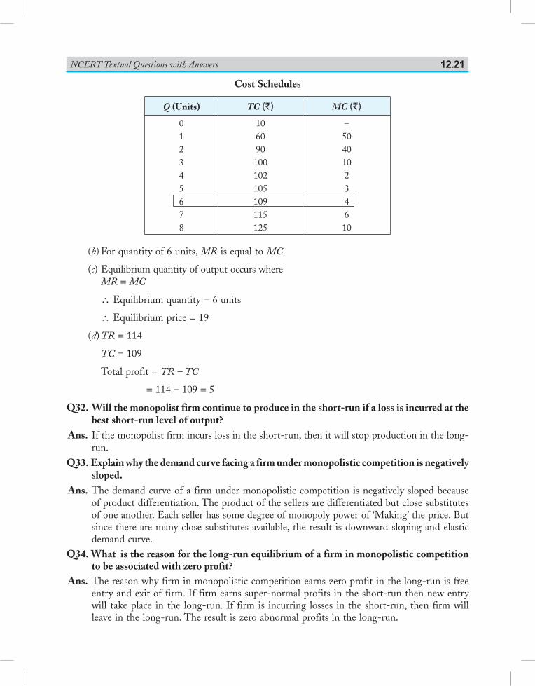
NCERT Textual Questions with Answers 12.21
Cost Schedules
Q (Units) TC (`) MC (`)
012345678
106090100102105109115125
–504010234610
(b) For quantity of 6 units, MR is equal to MC.
(c) Equilibrium quantity of output occurs where MR = MC
\ Equilibrium quantity = 6 units
\ Equilibrium price = 19
(d) TR = 114
TC = 109
Total profit = TR – TC
= 114 – 109 = 5
Q32. Will the monopolist firm continue to produce in the short-run if a loss is incurred at the best short-run level of output?
Ans. If the monopolist firm incurs loss in the short-run, then it will stop production in the long-run.
Q33. Explain why the demand curve facing a firm under monopolistic competition is negatively sloped.
Ans. The demand curve of a firm under monopolistic competition is negatively sloped because of product differentiation. The product of the sellers are differentiated but close substitutes of one another. Each seller has some degree of monopoly power of ‘Making’ the price. But since there are many close substitutes available, the result is downward sloping and elastic demand curve.
Q34. What is the reason for the long-run equilibrium of a firm in monopolistic competition to be associated with zero profit?
Ans. The reason why firm in monopolistic competition earns zero profit in the long-run is free entry and exit of firm. If firm earns super-normal profits in the short-run then new entry will take place in the long-run. If firm is incurring losses in the short-run, then firm will leave in the long-run. The result is zero abnormal profits in the long-run.
Saraswati Introductory Microeconomics12.22
Q35. List the three different ways in which oligopoly firms may behave. Ans. Oligopoly firm may: (a) Cooperate with each other and formally have a contract or written document of their
policies. (b) Cooperate with each other but have tacit (informal) understanding. (c) Not cooperate with each other. Q36. What is meant by prices being rigid? How can oligopoly behaviour lead to such an
outcome? Ans. Rigid prices means that even if cost or demand changes there will be no change in the price
of the commodity. Oligopoly behaviour leads to such rigid/ constant/ sticky prices because: (a) firm have fair and satisfactory profit margin in the price. Small changes in cost and demand
get adjusted in the profit margin. (b) The unit of changing prices in terms of printing new price lists, advertising cost, cost of
informing the consumers, etc. is more. It discourages the firms to make changes in the price.
(c) Firms fear rival firm’s reactions. Firms are guided by long-term objectives and do not want to change the prevailing price.
oo

Practice Papers Based on CBSE Latest Question Paper Design

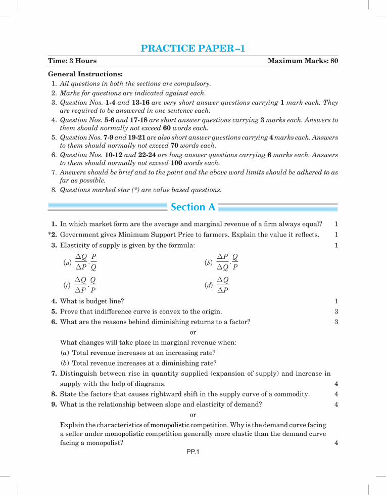
PRACTICE PAPER–1Time: 3 Hours Maximum Marks: 80
General Instructions: 1. All questions in both the sections are compulsory. 2. Marks for questions are indicated against each. 3. Question Nos. 1-4 and 13-16 are very short answer questions carrying 1 mark each. They
are required to be answered in one sentence each. 4. Question Nos. 5-6 and 17-18 are short answer questions carrying 3 marks each. Answers to
them should normally not exceed 60 words each. 5. Question Nos. 7-9 and 19-21 are also short answer questions carrying 4 marks each. Answers
to them should normally not exceed 70 words each. 6. Question Nos. 10-12 and 22-24 are long answer questions carrying 6 marks each. Answers
to them should normally not exceed 100 words each. 7. Answers should be brief and to the point and the above word limits should be adhered to as
far as possible. 8. Questions marked star (*) are value based questions.
Section A 1. Inwhichmarketformaretheaverageandmarginalrevenueofafirmalwaysequal? 1
*2. GovernmentgivesMinimumSupportPricetofarmers.Explainthevalueitreflects. 1
3. Elasticityofsupplyisgivenbytheformula: 1
(a) DD
QP
PQ
. (b) DD
PQ
QP
.
(c) DD
QP
QP
. (d) DD
QP
4.Whatisbudgetline? 1 5. Provethatindifferencecurveisconvextotheorigin. 3 6.Whatarethereasonsbehinddiminishingreturnstoafactor? 3
or Whatchangeswilltakeplaceinmarginalrevenuewhen: (a) Total revenueincreasesatanincreasingrate? (b) Totalrevenueincreasesatadiminishingrate?
7. Distinguishbetweenriseinquantitysupplied(expansionofsupply)andincreasein supplywiththehelpofdiagrams. 4 8. Statethefactorsthatcausesrightwardshiftinthesupplycurveofacommodity. 4 9.Whatistherelationshipbetweenslopeandelasticityofdemand? 4
or Explainthecharacteristicsofmonopolisticcompetition.Whyisthedemandcurvefacing
asellerundermonopolisticcompetitiongenerallymoreelasticthanthedemandcurve facingamonopolist? 4
PP.1
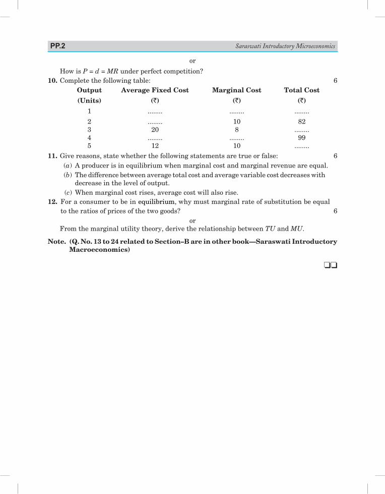
or
HowisP = d = MRunderperfectcompetition? 10.Completethefollowingtable: 6 Output Average Fixed Cost Marginal Cost Total Cost (Units) (`) (`) (`) 1 ........ ........ ........
2 ........ 10 82 3 20 8 ........ 4 ........ ........ 99 5 12 10 ........ 11.Givereasons,statewhetherthefollowingstatementsaretrueorfalse: 6 (a) Aproducerisinequilibriumwhenmarginalcostandmarginalrevenueareequal. (b) Thedifferencebetweenaveragetotalcostandaveragevariablecostdecreaseswith
decreaseinthelevelofoutput. (c)Whenmarginalcostrises,averagecostwillalsorise.12.Foraconsumertobeinequilibrium,whymustmarginalrateofsubstitutionbeequal totheratiosofpricesofthetwogoods? 6
or Fromthemarginalutilitytheory,derivetherelationshipbetweenTU and MU.
Note. (Q. No. 13 to 24 related to Section–B are in other book—Saraswati Introductory Macroeconomics)
oo
Saraswati Introductory MicroeconomicsPP.2
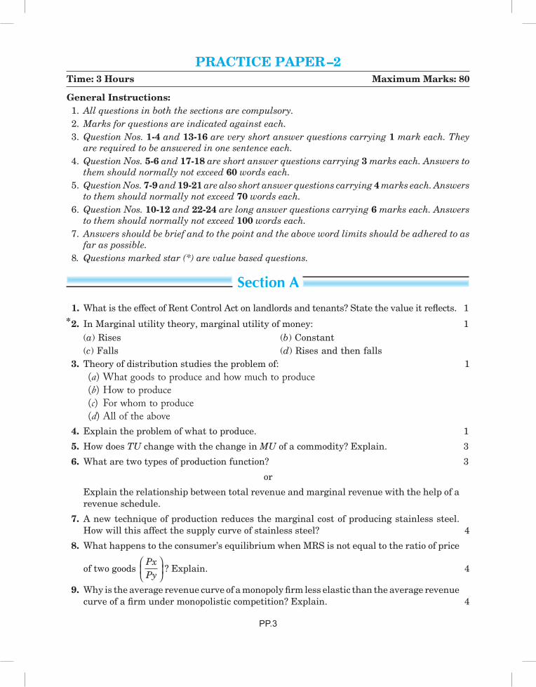
PRACTICE PAPER–2Time: 3 Hours Maximum Marks: 80
General Instructions: 1. All questions in both the sections are compulsory. 2. Marks for questions are indicated against each. 3. Question Nos. 1-4 and 13-16 are very short answer questions carrying 1 mark each. They
are required to be answered in one sentence each. 4. Question Nos. 5-6 and 17-18 are short answer questions carrying 3 marks each. Answers to
them should normally not exceed 60 words each. 5. Question Nos. 7-9 and 19-21 are also short answer questions carrying 4 marks each. Answers
to them should normally not exceed 70 words each. 6. Question Nos. 10-12 and 22-24 are long answer questions carrying 6 marks each. Answers
to them should normally not exceed 100 words each. 7. Answers should be brief and to the point and the above word limits should be adhered to as
far as possible. 8. Questions marked star (*) are value based questions.
Section A
1.WhatistheeffectofRentControlActonlandlordsandtenants?Statethevalueitreflects. 1
2. In Marginal utility theory, marginal utility of money: 1 (a) Rises (b) Constant (c) Falls (d) Rises and then falls 3. Theory of distribution studies the problem of: 1 (a) What goods to produce and how much to produce (b) How to produce (c) For whom to produce (d) All of the above 4. Explain the problem of what to produce. 1
5. How does TU change with the change in MU of a commodity? Explain. 3
6. What are two types of production function? 3
or
Explain the relationship between total revenue and marginal revenue with the help of a revenue schedule.
7. A new technique of production reduces the marginal cost of producing stainless steel. How will this affect the supply curve of stainless steel? 4
8. What happens to the consumer’s equilibrium when MRS is not equal to the ratio of price
of two goods PxPy
? Explain. 4
9.Whyistheaveragerevenuecurveofamonopolyfirmlesselasticthantheaveragerevenue curveofafirmundermonopolisticcompetition?Explain. 4
PP.3
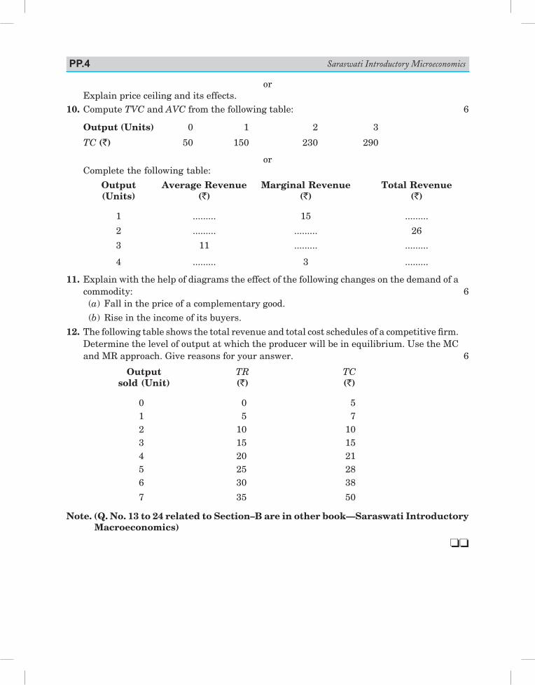
or Explain price ceiling and its effects. 10. Compute TVC and AVC from the following table: 6
Output (Units) 0 1 2 3
TC (`) 50 150 230 290
or Complete the following table:
Output Average Revenue Marginal Revenue Total Revenue (Units) (`) (`) (`)
1 ......... 15 .........
2 ......... ......... 26
3 11 ......... .........
4 ......... 3 .........
11. Explain with the help of diagrams the effect of the following changes on the demand of a commodity: 6 (a) Fall in the price of a complementary good. (b) Rise in the income of its buyers. 12.Thefollowingtableshowsthetotalrevenueandtotalcostschedulesofacompetitivefirm.
Determine the level of output at which the producer will be in equilibrium. Use the MC and MR approach. Give reasons for your answer. 6
Output TR TC sold (Unit) (`) (`)
0 0 5 1 5 7 2 10 10 3 15 15 4 20 21 5 25 28 6 30 38
7 35 50
Note. (Q. No. 13 to 24 related to Section–B are in other book—Saraswati Introductory Macroeconomics)
oo
Saraswati Introductory MicroeconomicsPP.4
PRACTICE PAPER–3Time: 3 Hours Maximum Marks: 80
General Instructions: 1. All questions in both the sections are compulsory. 2. Marks for questions are indicated against each. 3. Question Nos. 1-4 and 13-16 are very short answer questions carrying 1 mark each. They
are required to be answered in one sentence each. 4. Question Nos. 5-6 and 17-18 are short answer questions carrying 3 marks each. Answers to
them should normally not exceed 60 words each. 5. Question Nos. 7-9 and 19-21 are also short answer questions carrying 4 marks each. Answers
to them should normally not exceed 70 words each. 6. Question Nos. 10-12 and 22-24 are long answer questions carrying 6 marks each. Answers
to them should normally not exceed 100 words each. 7. Answers should be brief and to the point and the above word limits should be adhered to as
far as possible. 8. Questions marked star (*) are value based questions.
Section A *1. Government has enacted consumer protection act for protecting the rights of consumers. State the value it refl ects. 1
2. What kind of relationship exists between demand for a good and price of its substitute goods? 1
(a) Direct (b) Inverse
(c) No effect (d) Can be direct or inverse
3. In Marginal utility theory, marginal utility of money: 1 (a) Rises (b) Constant (c) Falls (d) Rises and then falls 4. State the law of demand. 1
5. What do you understand by returns to a factor? State the reasons for diminishing returns to a factor. 3
or What would be the shape of the AR curve when total revenue curve is:
(a) Positively sloped straight line passing through the origin? (b) A horizontal line?
6. How does availability of substitutes infl uence its price elasticity of demand? 3
7. Explain what happens to the profi t in the long-run if the fi rms are free to enter the industry. 4
8. Using geometric method, compare price elasticity of demand at a price when two straight downward sloping demand curves are parallel to each other. 4
PP.5
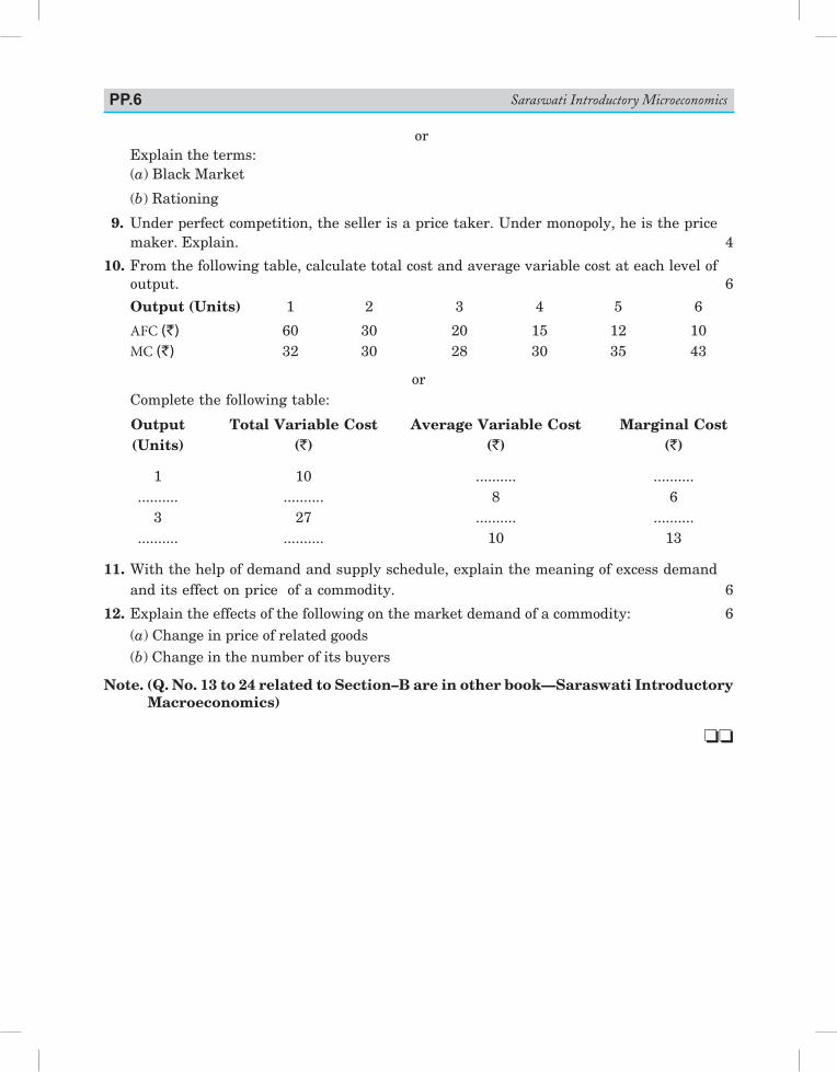
or Explain the terms: (a) Black Market
(b) Rationing
9. Under perfect competition, the seller is a price taker. Under monopoly, he is the price maker. Explain. 4
10. From the following table, calculate total cost and average variable cost at each level of output. 6
Output (Units) 1 2 3 4 5 6
AFC (`) 60 30 20 15 12 10 MC (`) 32 30 28 30 35 43
or Complete the following table:
Output Total Variable Cost Average Variable Cost Marginal Cost (Units) (`) (`) (`)
1 10 .......... .......... .......... .......... 8 6 3 27 .......... .......... .......... .......... 10 13
11. With the help of demand and supply schedule, explain the meaning of excess demand and its effect on price of a commodity. 6
12. Explain the effects of the following on the market demand of a commodity: 6 (a) Change in price of related goods (b) Change in the number of its buyers
Note. (Q. No. 13 to 24 related to Section–B are in other book—Saraswati Introductory Macroeconomics)
oo
Saraswati Introductory MicroeconomicsPP.6
PRACTICE PAPER–4Time: 3 Hours Maximum Marks: 80
General Instructions: 1. All questions in both the sections are compulsory. 2. Marks for questions are indicated against each. 3. Question Nos. 1-4 and 13-16 are very short answer questions carrying 1 mark each. They
are required to be answered in one sentence each. 4. Question Nos. 5-6 and 17-18 are short answer questions carrying 3 marks each. Answers to
them should normally not exceed 60 words each. 5. Question Nos. 7-9 and 19-21 are also short answer questions carrying 4 marks each. Answers
to them should normally not exceed 70 words each. 6. Question Nos. 10-12 and 22-24 are long answer questions carrying 6 marks each. Answers
to them should normally not exceed 100 words each. 7. Answers should be brief and to the point and the above word limits should be adhered to as
far as possible. 8. Questions marked star (*) are value based questions.
Section A 1. Governmentprovidessubsidytofarmersonfertilizers.Explainthevalueitreflects. 1
2. Coefficientofelasticityofdemandisnegative.Itmeans: 1
(a)Consumerssometimesbuynegativeunitsofacommodity (b)Priceandquantitydemandedmoveinsamedirection (c) Law of demand holds (d)Thetwogoodsarecomplementarytoeachother
3.Whatkindofrelationshipexistsbetweendemandforagoodandpriceof itssubstitutegoods? 1
(a)Direct (b)Inverse
(c) Noeffect (d)Canbedirectorinverse 4. State the law of supply. 1
5. IfPX = 4, PY = 2, MRSXY=1.Istheconsumerinequilibrium? 3
6. Givethreeassumptionsofproductionpossibilityfrontier. 3or
Explain‘interdependenceamongfirms’inanoligopolymarket.
7.WhatarethesimilaritiesanddifferencesbetweenTVC and MCcurves? 4
8. Give the relationship between TR, AR and MRcurveunderMonopoly. 4
9. Drawlinearsupplycurveshowingdifferentvaluesofelasticityofsupply. 4
or Howdoestaxinfluencethesupplyofagoodbyafirm?Explain.
PP.7
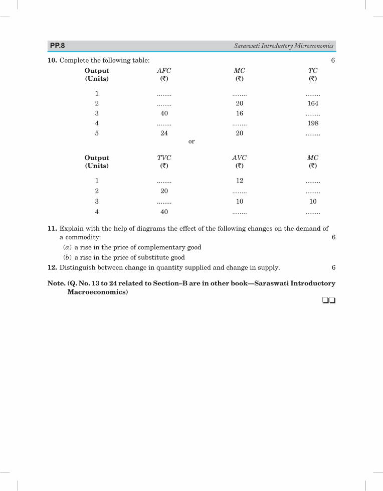
10.Completethefollowingtable: 6
Output AFC MC TC (Units) (`) (`) (`)
1 ........ ........ ........ 2 ........ 20 164 3 40 16 ........ 4 ........ ........ 198 5 24 20 ........
or
Output TVC AVC MC (Units) (`) (`) (`)
1 ........ 12 ........
2 20 ........ ........
3 ........ 10 10
4 40 ........ ........
11.Explainwiththehelpofdiagramstheeffectofthefollowingchangesonthedemandof acommodity: 6 (a) ariseinthepriceofcomplementarygood (b) ariseinthepriceofsubstitutegood 12.Distinguishbetweenchangeinquantitysuppliedandchangeinsupply. 6
Note. (Q. No. 13 to 24 related to Section–B are in other book—Saraswati Introductory Macroeconomics)
oo
Saraswati Introductory MicroeconomicsPP.8
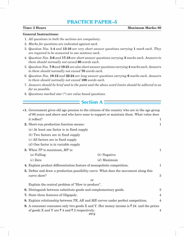
PRACTICE PAPER–5Time: 3 Hours Maximum Marks: 80
General Instructions: 1. All questions in both the sections are compulsory. 2. Marks for questions are indicated against each. 3. Question Nos. 1-4 and 13-16 are very short answer questions carrying 1 mark each. They
are required to be answered in one sentence each. 4. Question Nos. 5-6 and 17-18 are short answer questions carrying 3 marks each. Answers to
them should normally not exceed 60 words each. 5. Question Nos. 7-9 and 19-21 are also short answer questions carrying 4 marks each. Answers
to them should normally not exceed 70 words each. 6. Question Nos. 10-12 and 22-24 are long answer questions carrying 6 marks each. Answers
to them should normally not exceed 100 words each. 7. Answers should be brief and to the point and the above word limits should be adhered to as
far as possible. 8. Questions marked star (*) are value based questions.
Section A 1. Government gives old age pension to the citizens of the country who are in the age group
of 60 years and above and who have none to support or maintain them. What value does itreflect? 1
2. Short-run production function means: 1
(a) At least one factor is in fixed supply
(b) Two factors are in fixed supply (c) All factors are in fixed supply (d) One factor is in variable supply
3. When TP is maximum, MP is: 1 (a) Falling (b) Negative
(c) Zero (d) Maximum
4. Explain product differentiation feature of monopolistic competition. 1
5. Defineanddrawaproductionpossibilitycurve.Whatdoesthemovementalongthiscurveshow? 3
or Explain the central problem of “How to produce”.
6. Distinguish between substitute goods and complementary goods. 3
7. State three features of Oligopoly. 4
8. Explain relationship between TR, AR and MR curves under perfect competition. 4
9. A consumer consumes only two goods X and Y. Her money income is ` 24 and the prices of goods X and Y are ` 4 and ` 2 respectively. 4
PP.9
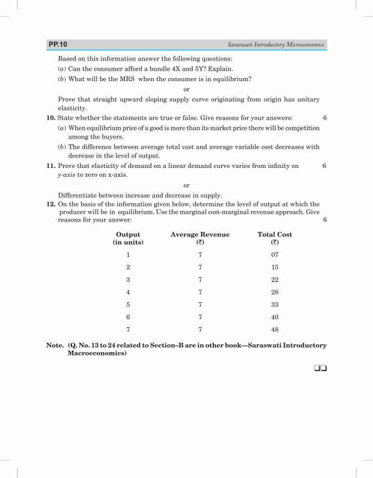
Based on this information answer the following questions:
(a)Cantheconsumeraffordabundle4Xand5Y?Explain.
(b)WhatwillbetheMRSwhentheconsumerisinequilibrium?
or
Prove that straight upward sloping supply curve originating from origin has unitary elasticity.
10. State whether the statements are true or false. Give reasons for your answers: 6
(a) When equilibrium price of a good is more than its market price there will be competition among the buyers.
(b) The difference between average total cost and average variable cost decreases with decrease in the level of output.
11.Provethatelasticityofdemandonalineardemandcurvevariesfrominfinityon 6 y-axis to zero on x-axis.
or
Differentiate between increase and decrease in supply. 12. On the basis of the information given below, determine the level of output at which the
producer will be in equilibrium. Use the marginal cost-marginal revenue approach. Give reasons for your answer: 6
Output Average Revenue Total Cost (in units) (`) (`)
1 7 07
2 7 15
3 7 22
4 7 28
5 7 33
6 7 40
7 7 48
Note. (Q. No. 13 to 24 related to Section–B are in other book—Saraswati Introductory Macroeconomics)
oo
Saraswati Introductory MicroeconomicsPP.10
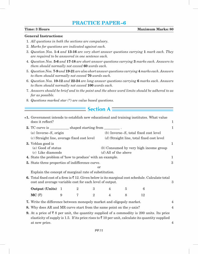
PRACTICE PAPER–6Time: 3 Hours Maximum Marks: 80
General Instructions: 1. All questions in both the sections are compulsory. 2. Marks for questions are indicated against each. 3. Question Nos. 1-4 and 13-16 are very short answer questions carrying 1 mark each. They
are required to be answered in one sentence each. 4. Question Nos. 5-6 and 17-18 are short answer questions carrying 3 marks each. Answers to
them should normally not exceed 60 words each. 5. Question Nos. 7-9 and 19-21 are also short answer questions carrying 4 marks each. Answers
to them should normally not exceed 70 words each. 6. Question Nos. 10-12 and 22-24 are long answer questions carrying 6 marks each. Answers
to them should normally not exceed 100 words each. 7. Answers should be brief and to the point and the above word limits should be adhered to as
far as possible. 8. Questions marked star (*) are value based questions.
Section A 1. Government intends to establish new educational and training institutes. What value
doesitreflect? 1
2. TC curve is ___________ shaped starting from _________ . 1 (a) Inverse–S, origin (b) Inverse–S, total fixed cost level (c) Straight line, average fixed cost level (d) Straight line, total fixed cost level
3. Veblan good is 1 (a) Good of status (b) Consumed by very high income group (c) Like diamonds (d) All of the above 4. State the problem of ‘how to produce’ with an example. 1
5. State three properties of indifference curve. 3or
Explain the concept of marginal rate of substitution.
6. Totalfixedcostofafirmis̀ 12. Given below is its marginal cost schedule. Calculate total cost and average variable cost for each level of output. 3
Output (Units) 1 2 3 4 5 6
MC (`) 9 7 2 4 8 12
7. Write the difference between monopoly market and oligopoly market. 4
8. Why does AR and MR curve start from the same point on the y-axis? 4
9. At a price of ` 8 per unit, the quantity supplied of a commodity is 200 units. Its price elasticity of supply is 1.5. If its price rises to ̀ 10 per unit, calculate its quantity supplied
at new price. 4
PP.11
or
Distinguishbetweenfixedcostandvariablecost.Give2examplesforeach.
10. Explain the law of variable proportions. Use diagram. 6
or
Whatismeantbyreturnstoafactor?Statethelawofdiminishingreturnstoafactor.
11. Explain producer’s equilibrium using a schedule. Use MR and MC approach. 6
12. Explain with the help of a diagram the effect of rightward shift of the supply curve of a commodity on its equilibrium price and quantity. 6
Note. (Q. No. 13 to 24 related to Section–B are in other book—Saraswati Introductory Macroeconomics)
oo
Saraswati Introductory MicroeconomicsPP.12
PRACTICE PAPER–7Time: 3 Hours Maximum Marks: 80
General Instructions: 1. All questions in both the sections are compulsory. 2. Marks for questions are indicated against each. 3. Question Nos. 1-4 and 13-16 are very short answer questions carrying 1 mark each. They
are required to be answered in one sentence each. 4. Question Nos. 5-6 and 17-18 are short answer questions carrying 3 marks each. Answers to
them should normally not exceed 60 words each. 5. Question Nos. 7-9 and 19-21 are also short answer questions carrying 4 marks each. Answers
to them should normally not exceed 70 words each. 6. Question Nos. 10-12 and 22-24 are long answer questions carrying 6 marks each. Answers
to them should normally not exceed 100 words each. 7. Answers should be brief and to the point and the above word limits should be adhered to as
far as possible. 8. Questions marked star (*) are value based questions.
Section A 1.WhatvaluedoesthegovernmentpolicytosurrendertoyourLPGsubsidyreflect? 1
2. AR is always equal to ___________. 1
(a) Revenue (b) Price
(c) Cost (d) Profit
3. Factor which affects market demand but not individual demand can be: 1
(a) Number of consumers in the market (b) Age and sex composition of population (c) Distribution of income (d) All of the above 4. Explain the meaning of opportunity cost. 1
5. When the price of a good rises from ` 5 per unit to ` 6 per unit, its demand fall from 20 units to 10 units. Compare expenditures on the good to determine whether demand is
elastic or inelastic. 3
6. Given the market price of a good, how does a consumer decide as to how many units of thatgoodtobuy?Explain. 3
or
For one commodity explain consumers equilibrium with the help of a schedule.
7. Suppose there is technology improvement is our country. How does it affect production possibilitiesinourcountry? 4
8. Explain three features of Perfect Competition. 4
PP.13
or Findthemaximumprofitpositionfromthefollowingdata: Output (Units) TR (`) TC (`) 1 10 12 2 18 20 3 24 24 4 21 36 5 18 50 Isthemaximumprofitlevelnormalorabnormal?Givereasonforyouranswer.
9. What will be the price elasticity of supply at any point on a straight line curve if: 4 (a)Supplycurveintersectsonx-axisinitsnegativerange? (b)Supplycurveintersectsonx-axisinitspositiverange? (c) Supplycurvepassesthroughtheorigin?
10.Whatwillbetheeffectofthefollowingchangesintotalrevenueormarginalrevenue? 6 (a) Average revenue is constant. (b) Total revenue increases at a constant rate.
11. Explain producer’s equilibrium through MR and MC schedule and conditions. 6
12.Howistheequilibriumpriceofagooddetermined?Explainwiththehelpofadiagrama situation when both demand and supply curves shift to the right but equilibrium
price remains the same. 6or
Explain the implications of the following: (a) Thefeatureoffreeentryandexitofthefirmsunderperfectcompetition. (b) Only one seller in the market.
Note. (Q. No. 13 to 24 related to Section–B are in other book—Saraswati Introductory Macroeconomics)
oo
Saraswati Introductory MicroeconomicsPP.14

Project Work 1. A report on demographic structure of your neighbourhood. 2. Changing consumer awareness amongst households. 3. Dissemination of price information for growers and its impact on
consumers. 4. Study of a cooperative institution: milk cooperatives, marketing
cooperatives, etc. 5. Case studies on public private partnership, outsourcing and
outward Foreign Direct Investment. 6. Global warming. 7. Designing eco-friendly projects applicable in school such as paper
and water recycle. 8. Cartels 9. Price Discrimination 10. Monopolistic Competition and Social Waste 11. Oligopolistic Firms in a Prisoner’s Dilemma 12. Case Study of Cartel—Organisation of Petroleum Exporting
Countries (OPEC) 13. Minimum Wage Law 14. Rent Control Act 15. Elasticity of Demand—Case Study of Newspaper 16. Minimum Support Price 17. Price Effect and Indifference Curve 18. Geometric Method of Finding Point Elasticity of Demand 19. Equilibrium Under Monopoly 20. Comparison of Price and Output Under Monopoly and Perfect
Competition

Project-1: A report on demographic structure of your neighbourhood.
Introduction. Demographic structure is an important aspect of any socio-economic survey and it is important for all developmental activities.
Objective: This survey and the resultant report will help to relate the theoretical aspects read by you in economics textbooks with the real situation. There are many dimensions that must be taken care of while conducting any survey and reporting the findings of such a survey. These include: (i) Scope and objective of the survey. (ii) Selecting a representative sample from the population. Representative here means
that the sample chosen should be reflective of all the features and characteristics of the population from which it is taken.
(iii) Finalisation and pretesting of the questionnaire. (iv) Collection of data. (v) Analysis and Report writing.
Steps of survey. For conducting such a survey, follow these steps: 1. Choose a locality of your interest and take a sample of about 40 to 50 households.
Make sure that the households are not homogeneous. That is, the households chosen must be a mixed basket of rich, poor, lower-middle class and upper-middle class families.
2. Make a questionnaire taking into account the fact that the alternate responses to the questions should cover all the expected choices of the respondents.
3. Demographic features include gender, age, knowledge of languages, disabilities, employment status, and many more things. You should include all these features in the questions of the questionnaire.
4. Patterns of consumption of the households are analysed by using the data and information on their expenditure on different commodities. In theory, we say that marginal propensity to spend by the poor people tend to be more as compared to the rich people. Also, expenditure on comforts and luxuries increases as income rises. So, these theoretical aspects can be verified from the observations and findings of the survey. The expenditure can be depicted as the proportion of income spent on various items of necessities, luxuries and comforts.
5. The occupational structure of a society reveals the distribution of people among different occupations or economic activities. The study of occupational struture is sociologically an important aspect because of its effects on social class and other forms of social inequality. Different occupations in which the people in a locality may be involved can be teaching, financial services, professionals, agriculture, industries, etc.
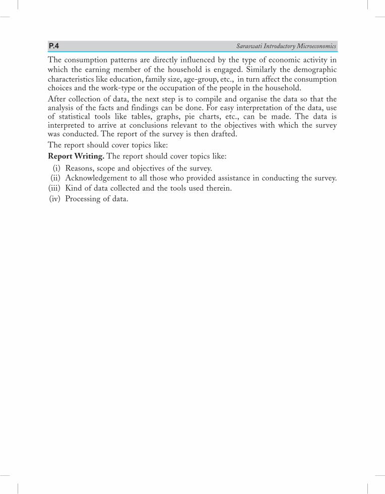
Saraswati Introductory MicroeconomicsP.4
The consumption patterns are directly influenced by the type of economic activity in which the earning member of the household is engaged. Similarly the demographic characteristics like education, family size, age-group, etc., in turn affect the consumption choices and the work-type or the occupation of the people in the household. After collection of data, the next step is to compile and organise the data so that the analysis of the facts and findings can be done. For easy interpretation of the data, use of statistical tools like tables, graphs, pie charts, etc., can be made. The data is interpreted to arrive at conclusions relevant to the objectives with which the survey was conducted. The report of the survey is then drafted. The report should cover topics like:Report Writing. The report should cover topics like:
(i) Reasons, scope and objectives of the survey. (ii) Acknowledgement to all those who provided assistance in conducting the survey. (iii) Kind of data collected and the tools used therein. (iv) Processing of data.

Project-2: Changing consumer awareness amongst households.
Introduction. Through this project, the students intend to find out the level of consumer awareness amongst household of their locality by conducting a survey and analysing its results. The findings will show how many people are well aware of consumer rights. Further, the survey will also enable to find out the methods through which awareness can be widely spread, e.g., What are their rights, Is there any violation of such rights and What are the remedies available to them.
Objective: Based upon the introduction above, students can pointwise list down the objectives of the project including the fact that the level of consumer awareness is changing day by day.Scope. Here the students can mention that how this project/survey will bring awareness among the people.Population Size. Depending upon the number of households, students can decide the favourable number of respondents. Ideally it should be at least 50 households. Source of Data Collection. In the present project it will be primary data which will be collected through administering the questionnaire.Method of Data Collection. For the sake of convenience, students can opt for sample survey.Questionnaire. A sample questionnaire is given below for the students. They can prepare their own questionnaire based on this. The students are advised to pretest the questionnaire before administering it to the entire population.Conducting the Survey/Collection of Data. After marking corrections/removing anamolies from the questionnaire, students can use it to collect data.Processing, Classifying and Analysing the Collected Data. Now process the data, classify it and analyse the findings. Trace the trends, facts, etc.Prepare the Project Report. Prepare a detailed report covering the following points. 1. Percentage of people who are conscious about products. 2. Percentage of people who are aware of the consumer rights. 3. How many people reported violation in their rights? 4. To whom did they address their grievances? 5. What were the outcome of their efforts? 6. How many consumers resorted to legal measures?Likewise the students can analyse the data and bring out the concrete facts about the awareness of consumer rights. They can fetch many more interpretations according to their wisdom. Presentation. Students can also make a power point presentation and present it in front of the whole class.

Saraswati Introductory MicroeconomicsP.6
Specimen QuestionnaireSection-A
Personal Information 1. Name ......................................................................... 1. (a) Male/Female .................
2. Address........................................................................................ State ......................
3. Age/Date of birth .......................................................................................................
4. Marital Status Married/Unmarried/Divorcee/Widow
5. Marriage Anniversary .................................................................................................
6. Education ...................................................................................................................
7. Employed/Unemployed ............................................................................................
8. If Employed, Please state your Profession ..................................................................
9. Monthly Income ........................................................................................................ 10. Do you own (a) Car (b) Credit card (c) Own house (Mark üwhichever applies) 11. Phone Number ........................................................................................................... 12. Mobile Number ..........................................................................................................
13. E-mail ID ...................................................................................................................
Section-BSurvey Oriented Questions
(Please tick ü as appropriate)
Yes No
1. Who purchase all the household goods, you or your spouse?
Self Spouse2. Are you a brand conscious consumer?
3. Where do you purchase goods from
Local Grocer Branded store
Mall Others
------------- (please specify)4. Do you examine MRP before buying?
5. Do you get commodities on lesser price than MRP?
6. Do you check the quality of the commodity?
7. Do you check ingredients of the product at the time of purchase?
8. Do you check the expiry date of the products while purchasing?
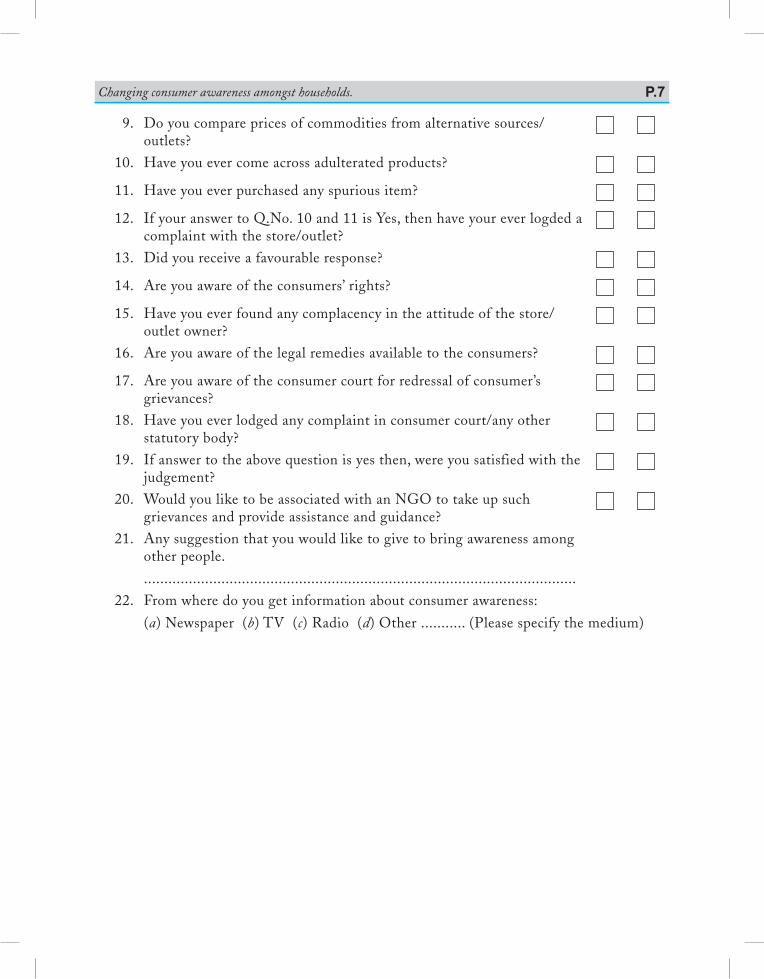
P.7Changing consumer awareness amongst households.
9. Do you compare prices of commodities from alternative sources/outlets?
10. Have you ever come across adulterated products?
11. Have you ever purchased any spurious item?
12. If your answer to Q.No. 10 and 11 is Yes, then have your ever logded a complaint with the store/outlet?
13. Did you receive a favourable response?
14. Are you aware of the consumers’ rights?
15. Have you ever found any complacency in the attitude of the store/outlet owner?
16. Are you aware of the legal remedies available to the consumers?
17. Are you aware of the consumer court for redressal of consumer’s grievances?
18. Have you ever lodged any complaint in consumer court/any other statutory body?
19. If answer to the above question is yes then, were you satisfied with the judgement?
20. Would you like to be associated with an NGO to take up such grievances and provide assistance and guidance?
21. Any suggestion that you would like to give to bring awareness among other people.
..........................................................................................................22. From where do you get information about consumer awareness:
(a) Newspaper (b) TV (c) Radio (d) Other ........... (Please specify the medium)
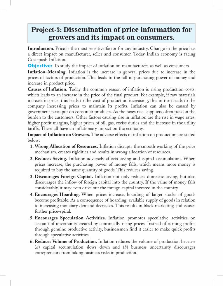
Project-3: Dissemination of price information for growers and its impact on consumers.
Introduction. Price is the most sensitive factor for any industry. Change in the price has a direct impact on manufacturer, seller and consumer. Today Indian economy is facing Cost-push Inflation.Objective: To study the impact of inflation on manufacturers as well as consumers.Inflation–Meaning. Inflation is the increase in general prices due to increase in the prices of factors of production. This leads to the fall in purchasing power of money and increase in product price.Causes of Inflation. Today the common reason of inflation is rising production costs, which leads to an increase in the price of the final product. For example, if raw materials increase in price, this leads to the cost of production increasing, this in turn leads to the company increasing prices to maintain its profits. Inflation can also be caused by government taxes put on consumer products. As the taxes rise, suppliers often pass on the burden to the customers. Other factors causing rise in inflation are the rise in wage rates, higher profit margins, higher prices of oil, gas, excise duties and the increase in the utility tariffs. These all have an inflationary impact on the economy. Impact of Inflation on Growers. The adverse effects of inflation on production are stated below: 1. Wrong Allocation of Resources. Inflation disrupts the smooth working of the price
mechanism, creates rigidities and results in wrong allocation of resources. 2. Reduces Saving. Inflation adversely affects saving and capital accumulation. When
prices increase, the purchasing power of money falls, which means more money is required to buy the same quantity of goods. This reduces saving.
3. Discourages Foreign Capital. Inflation not only reduces domestic saving, but also discourages the inflow of foreign capital into the country. If the value of money falls considerably, it may even drive out the foreign capital invested in the country.
4. Encourages Hoarding. When prices increase, hoarding of larger stocks of goods become profitable. As a consequence of hoarding, available supply of goods in relation to increasing monetary demand decreases. This results in black marketing and causes further price-spiral.
5. Encourages Speculation Activities. Inflation promotes speculative activities on account of uncertainty created by continually rising prices. Instead of earning profits through genuine productive activity, businessmen find it easier to make quick profits through speculative activities.
6. Reduces Volume of Production. Inflation reduces the volume of production because (a) capital accumulation slows down and (b) business uncertainty discourages entrepreneurs from taking business risks in production.
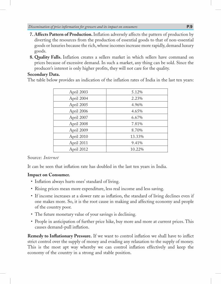
P.9Dissemination of price information for growers and its impact on consumers
7. Affects Pattern of Production. Inflation adversely affects the pattern of production by diverting the resources from the production of essential goods to that of non-essential goods or luxuries because the rich, whose incomes increase more rapidly, demand luxury goods.
8. Quality Falls. Inflation creates a sellers market in which sellers have command on prices because of excessive demand. In such a market, any thing can be sold. Since the producer’s interest is only higher profits, they will not care for the quality.
Secondary Data.The table below provides an indication of the inflation rates of India in the last ten years:
April 2003 5.12%April 2004 2.23%April 2005 4.96%April 2006 4.65%April 2007 6.67%April 2008 7.81%April 2009 8.70%April 2010 13.33%April 2011 9.41%April 2012 10.22%
Source: Internet
It can be seen that inflation rate has doubled in the last ten years in India.
Impact on Consumer. • Inflationalwayshurtsones’standardofliving.
• Risingpricesmeanmoreexpenditure,lessrealincomeandlesssaving.
• Ifincomeincreasesataslowerrateasinflation,thestandardoflivingdeclinesevenifone makes more. So, it is the root cause in making and affecting economy and people of the country poor.
• Thefuturemonetaryvalueofyoursavingsisdeclining.
• Peopleinanticipationoffurtherpricehike,buymoreandmoreatcurrentprices.Thiscauses demand-pull inflation.
Remedy to Inflationary Pressure. If we want to control inflation we shall have to inflict strict control over the supply of money and evading any relaxation to the supply of money. This is the most apt way whereby we can control inflation effectively and keep the economy of the country in a strong and stable position.
Saraswati Introductory MicroeconomicsP.10Project-4: Study of a cooperative institution: milk
cooperatives, marketing cooperatives, etc.
Introduction. India is the largest producer of milk in the world from 11 million tonnes in 1950-51, the production has increased to 121.84 million tonnes in 2010-11.
The successful production and marketing of milk and related products largely owes to the cooperative societies which have functioned efficiently and effectively and have given substantial growth momentum to this movement. The cooperative societies which are spread all across the country have become an important secondary source of income for millions of rural families and has assumed an important role in providing employment and income generating opportunities.
Milk cooperatives have procured 26.211 million metric tonnes milk in 2010-11 of the total national production of 166 million metric tonnes. There are a number of cooperative institutions engaged in the trading of milk which are successfully working.
For the present project we are taking up the milk cooperative “Kaira District Cooperative Milk Producer’s Union Limited” for the detailed study.
Background. Kaira District Cooperative Milk Producer’s Union Limited (KDCMPUL).
It is the first ever cooperative milk producer. Union was incorporated in 1946 in the Kheda district of Gujarat. Its founding chairman was a social worker Tribhoran Das Patel. Its success also known as Anand pattern led to creation of District Cooperative Milk Producers Union at every district. By June 1948 the KDCMPUL had started pasturizing milk of Bombay Milk Scheme.
In 1970 it started White Revolution in India. It popularly came to be known as Amul Dairy after its brand name.
Modus Operandi. Amul Dairy procures milk from around 1,163 member village cooperative societies (VCS) which consist of 6.35 lakh farmers which hold the entire shareholding of Amul.
Capacity. It has total milk producing capacity of 7.30 lakh metric tonns per annum.
Owned by. It is owned by Village Cooperative Society (VCS) having 1163 member villages.
Expanding Suppliers Base and Product Portfolio.
(a) Suppliers base has increased from 1113 member to 1163 member VCS from FY 2008 to FY 2011.
(b) Milk procurement has increased @ 8.70% during same period to 52 crores kg from 6.35 lakhs.
P.11Study of a cooperative institution: milk cooperatives, marketing cooperatives, etc
Strong Pricing Paid as seen higher price paid to members VCS. It has been the primary objective of the Dairy Processing Unions (DPUs) to pass on the maximum possible benefits to the members of VCS. The price paid in recent financial years are as follows:
Financial Year Price Paid to Farmers 2008-09 298/ kg fat 2010-11 391/kg fat 2011-12 428/kg fat
Liquidity Position. Its financial position is comfortable as it has maintained an average fixed deposit balance of around ` 50 crores for 12 months for the period ended 30 Sep 2011.It had a bank balance of ` 144 cr as on 31 March 2011.
Geographically Diversified Revenue Stream. It caters to entire Gujarat, it even supplies to Kolkata, Pune and Mumbai through its satellite dairies and packaging stations.Cooperative Structure and Entry Barrier for Private Players. Its cooperative structure is its strength which deters entry of private players. It is based on the fact that the farmer members who are supplier of milk are also the owners of D.P.Us.
Prospects. With modern manufacturing facilities, large supply base, diversified product mix and a strong market entity, it dominates dairy market with its brand ‘Amul’.Source: Credit Analysis and Research Limited Report.

Saraswati Introductory MicroeconomicsP.12Project-5: Case studies on public private partnership, outsourcing and outward Foreign Direct Investment.
Public Private Partnership–Meaning. The Government of India defines Public Private Partnership as:“An arrangement between a government / statutory entity / government owned entity on one side and a private sector entity on the other, for the provision of public assets and/or public services, through investments being made and/or management being undertaken by the private sector entity, for a specified period of time, where there is well defined allocation of risk between the priva te sector and the public entity and the private entity receives performance linked payments that conform (or are benchmarked) to specified and pre-determined performance standards, measurable by the public entity or its representative. “In projects that are aimed at creating public goods like in the infrastructure sector, the government may provide a capital subsidy in the form of a one-time grant, so as to make it more attractive to the private investors. In some other cases, the government may support the project by providing revenue subsidies, including tax breaks. These schemes are sometimes referred to as PPP, P3 or P3.Objective: Government organizations are looking for different ways of sourcing their activities to acquire various benefits. The objective of this project is to understand outsourcing and public-private partnerships (PPPs) as means of sourcing. Essential Conditions of PPP. • Arrangement with private sector entity. The asset and/or service under the contractual
arrangement will be provided by the Private Sector entity to the users. • Public asset or service for public benefit. The facilities/ services being provided are
traditionally provided by the Government, as a sovereign function, to the people. • Investments being made by and/or management undertaken by the private sector
entity. The arrangement could provide for financial investment and/or non-financial investment by the private sector.
• Operations or management for a specified period. The arrangement cannot be in perpetuity. After a pre-determined time period, the arrangement with the private sector entity comes to a closure.
• Risk sharing with the private sector. Mere outsourcing contracts are not PPPs. • Performance linked payments. The central focus is on performance and not merely
provision of facility or service. • Conformance to performance standards. The focus is on a strong element of service
delivery aspect and compliance to pre-determined and measurable standards to be specified by the Sponsoring Authority.
Various Models of PPP. • Build-operate-transfer(BOT) • Build-lease-transfer(BLT)

P.13Case studies on public private partnership, outsourcing and outward Foreign Direct Investment
• Design-build-operate-transfer(DBFOT) • Operate-maintain-transfer(OMT),etc. • Build-own-operate(BOO)CASE1: GMR’s TERMINAL 3 for DELHI AIRPORT:
A successful PPP model. Underinvestment in airport infrastructure since independence was a major cause for concern. Lack of funds and the expertise to develop and maintain the growing airport infrastructure needs of the country forced the government to invite private players to participate in infrastructure development under Public Private Partnership (PPP). It was in January 2006, that a consortium led by the GMR Group won the bid to develop the airport. Very soon, the PPP initiative yielded results, with two terminals being renovated and one new runway and terminal 1D being opened up for commercial operation. However, revolutionary change, as the experts called it, came about when the T3 was inaugurated on July 3, 2010. At the inauguration of T3, Manmohan Singh (Singh), Prime Minister of India, said, “The Delhi airport has improved its rank sharply in terms of Air Service Quality (ASQ) performance, from 101 in 2007 to 21 in 2010. After the opening of this new terminal we are hopeful that the airport will shortly rank within the first 10 airports of the world.”
Outsourcing–Meaning. Outsourcing is the contracting out of an internal business process to a third-party organisation, rather than staffing it internally is common in the modern economy. Outsourcing sometimes involves transferring employees and assets from one firm to another, but not always.
Outsourcing is said to help firms to perform well in their core competencies and mitigate shortage of skill or expertise in the areas where they want to outsource. Outsourcing can offer greater budget flexibility and control. Outsourcing lets organizations pay for only the services they need, when they need them. It also reduces the need to hire and train specialized staff, brings in fresh engineering expertise, and reduces capital and operating expenses.
CASE2: STATE HEALTH SOCIETY, BIHAR: A successful OUTSOURCING model
• Pathology Centres. In the government hospitals pathology services to the needy patients were not provided efficiently due to paucity of lab technicians and irregular supplies of reagents required for pathological tests. The State decided to outsource pathological services to reputed private labs in order to improve the pathological services in the government hospitals. Two agencies were selected through tender process. The agencies set up labs at the District hospitals and sample collection centres at the health facilities below district levels. In the State, 407 centres are operational. More than 4 lakh tests have been conducted in the last two years.
Saraswati Introductory MicroeconomicsP.14
• Radiology. In the State it has been decided to outsource radiology services in all the government health facilities. About 151 radiology centres have been operationalised. The centers have provided X-ray services to 3.53 lakh patients in the last two years. Ultrasound Facilities in the District Hospitals and Sub-divisional Hospital are also being provided.
• Hospital Maintenance Services. The support services for the cleanliness of the hospital’s wards and the premises were not up to the mark and the washing of the bed sheets, linen and other apparel were not proper due to paucity of adequate numbers of sweepers and washer- men. Due to recurrent power- cuts, the maintenance of the cold chain of the vaccines was also not proper. Similarly the diet given to the indoor patients were not satisfactory. In order to improve the support services in the hospitals, the State decided to outsource these services to private agencies and NGOs through tender process. The following support services have been outsourced:
1. Maintenance of Hospital Premises 2. Cleanliness of Hospitals 3. Laundry Services 4. 24 hrs. Generator Facility 5. Diet for Indoor Patients Outsourcing vs. PPP. Unlike outsourcing (such as hiring a security or cleaning company to do a job), a PPP entails the private party taking very substantial risk for financing a project’s capital and operating costs, designing and building a facility, and managing its operations to specified standards, normally over a significant period of time. Conclusion. A large number of interrelated factors are found as drivers for selecting the various sourcing arrangements. It is found that the strategic intents underlying the decision to implement a PPP or outsourcing arrangements differ from each other. Outsourcing is mainly used to reduce costs for non-core activities or to gain access to expertise otherwise out-of-reach and, while a shared services arrangement is selected when an organization wants to improve service levels and reduce costs at the same time. Finally, PPPs are focused on developing new and innovative services and seem to accomplish most intents at the expense of higher risks. The intents have relatively subtle differences, compared to how significantly the arrangements differ.CASE3: Outward FDIIt is now widely acknowledged that outward foreign direct investment (OFDI) can play an important role in cross-border knowledge flows in many industries. The home country tends to benefit from technological learning and knowledge spillovers if it invests in relatively innovation-intensive foreign countries. Also FDI host countries receive knowledge flows as inward FDI brings with it a bundle of knowledge assets in the form of new products, technologies, skills, managerial practices, new capital equipments, etc.
P.15Case studies on public private partnership, outsourcing and outward Foreign Direct Investment
CASE STUDY: Outward FDI (OFDI) by Indian Automotive firmsIndian automotive firms were observed to be early outward investors from Indian economy. Their OFDI activities started since early 1970s. Probably, India’s first automotive OFDI project was undertaken in 1972 by the Sah & Sanghi Group operating in the automobile distribution activities. A part of the group company, Bombay Auto Ancillary & Investments Private Limited, entered into a joint venture in Malaysia with about US $0.23 million for 35.7 per cent ownership. The year 1977 saw three Indian joint ventures abroad, one each directed at Malaysia, Kenya and Singapore. Bolton India invested US $0.18 million for 45 per cent equity interest in Auto Ancillaries Limited, Nairobi for manufacturing auto springs for Kenya’s motor vehicle assemblers.
Clearly the initial OFDI projects from Indian automotive sector are more into manufacturing activities and involve local partners in host developing countries.
Since the principal mode of their OFDI activities was joint venture, it can be argued that such Indian automotive OFDI has in fact transferred adapted knowledge that these firms have gained in localizing their production in India.
The participation of Indian automotive company in cross-border knowledge flows of intermediate technologies continued in 1980s with a number of new entrants and diversification into developed countries like USA, Germany and Greece. During 1980-89, a total of six Indian companies undertook an aggregate investment of US $0.82 million in 6 overseas joint venture and subsidiaries. OFDI during 1980s represents a group of new Indian automotive firms like Ashok Leyland, Bajaj, Autolite India, Mahindra & Mahindra and Scooters India joining overseas investment activities.
In 1981, Mahindra & Mahindra invested US$ 0.28 million in K.Zaharopoulos – an Athens-based Greek industrial and trading company for 55.47 per cent equity stake.
Case Study of Tata Group and Automotive OFDI
All OFDI activities by Tata Motors so far have been in commercial vehicles segment – trucks and buses, except that of Jaguar Land Rover in 2008 in the passenger car segment. Tata Motors have been producing commercial vehicles since 1954. While they have been producing cars in India since 1991 in foreign collaborations, their car manufacturing operations really started in a significant way in 1999 with ‘Indica’ production, an indigenously developed car; by 2007 Tata Motors had rolled over one million passenger cars off the Indica platform. The brand name and company name counts a lot in the passenger car segment. Tata Motors have earlier made marketing alliances with MG Rover, UK (starging 2002) and Khondro for the exports of Tata cars and with Rover/Phoenix Ventures for utility vehicles/pick-ups, however, with the sales being under the collaborator’s brand name. We believe that the acquisition of Land Rover and Jaguar is going to give Tata Motors the much needed global visibility in the passanger car segment, even though the Tata Motors has announced that the Rover and Jaguar brands would be taken forward.

Saraswati Introductory MicroeconomicsP.16Project-6: Global Warming.
Global Warming–Meaning. Global warming is the observed and projected increase in the average temperature of the Earth’s atmosphere and oceans. From global warming we expect a rise of the average temperature leading to–among other things–melting of glaciers and melting of the polar ice, increase of the mean sea level as well as generally more of extreme weather events and nature disasters like droughts, floods, tornadoes, etc.
Objective: To understand global warming, its impact on earth and mankind and the remedial measures to control its impact.
Global Warming Predictions. According to different assumptions about the future behaviour of mankind, a projection of current trends as represented by a number of different scenarios gives temperature increases of about 3° to 5°C (5° to 9° Fahrenheit) by the year 2100 or soon afterwards. A 3°C or 5° Fahrenheit rise would likely raise sea levels by about 25 meters (about 82 feet).
Factors Contributing to Global Warming. When it comes to knowing more about the causes of global warming, you need to look at the two main causes of global warming–natural causes and man-made causes.
1. Natural Causes of Global Warming (Uncontrollable). These are the causes of global warming that occur naturally over time on our planet, however many people don’t take notice of it.
• Oneofthemainnaturalcausesthataffectourplanetisthereleaseofmethanegasfromarctic tundra and wetlands. As you may already know, methane is a greenhouse gas and it is a very dangerous type of gas for our environment.
• Largevolcaniceruptionscanthrowsomuchdustintotheskythatthedustactsasashield to solar radiation and causes a cooling trend in the atmosphere.
• Whentherearechangesinthesolarradiationlevelsitcanhavesomeimpactontheearth’s climate. Increased solar activity can cause short-term warming cycles on the Earth.
• AstheEarthspinsonit’saxis,itdoesnotachieveperfectrotation.Itactuallywobblesa little, thus alternately exposing the northern and southern latitudes to more and less solar radiation. This wobble in the earth’s rotation has been causing changes in the temperature of the atmosphere for many millions of years.
2. Man-made Causes of Global Warming (Controllable). These are the factors made by man which contribute to the global warming. These can be controlled if one is determined to it.
• Man-madepollutionandmis-useoffossilfuelsisthemaincauseofglobalwarming.Whenhumansburnfossilfuels,thefossilfuelsreleaseagascalledCO2. Every time you get into your gas powered car you are burning fossil fuels, Industries are one of the biggest contributors of fossil fuel burning.

P.17Global warming
• Methaneisalsoanothercause;whenhumanbeingsminecoalordrillforoil,methaneisreleased into the atmosphere, and this is another real factor that causes global warming.
• Anotherverybigcauseofglobalwarmingisover-populationonourplanet.Therearejust too many people currently living on our small planet. The amount of food and water it takes to feed everyone is massive. To produce that food there are a lot of factors involved, such as transportation, feeding the livestock, machinery to process the food, etc.TheseallcauseemissionofCO2.
• Humans are also cutting down far too many trees, these are trees that convert ouratmosphericCO2 into oxygen, and we’re using the land that we cut the trees down from as property for our homes and buildings. This is probably one of the most important causes of global warming.
Impact of Global Warming. Following are the major threats of global warming to our ecological system:
• Most places will continue to get warmer, especially at night and in winter. The temperature change will benefit some regions while harming others — for example, patterns of tourism will shift. The warmer winters will improve health and agriculture in some areas, but globally, mortality will rise and food supplies will be endangered due to more frequent and extreme summer heat waves and other effects.
• Sea levels will continue to rise for many centuries. The last time the planet was 3°C warmer than now, the sea level was at least 6 meters (20 feet) higher that submerged coastlines where many millions of people now live, including cities from New York to Shanghai. The rise will probably be so gradual that later generations can simply abandon their parents’ homes, but a ruinously swift rise cannot be entirely ruled out.
• Weather patterns will keep changing towards an intensified water cycle with stronger floods and droughts. Most regions now subject to droughts will probably get drier(because of warmth as well as less precipitation), and most wet regions will get wetter. In particular, storms with more intense rainfall are liable to bring worse floods. Some places will get more snowstorms, but most mountain glaciers and winter snowpack will shrink, jeopardizing important water supply systems.
• Ecosystems will be stressed, uncounted valuable species, especially in the Arctic, mountainareas,andtropicalseas,mustshifttheirranges.Manythatcannotwillfaceextinction. A variety of pests and tropical diseases are expected to spread to warmed regions. These problems have already been observed in numerous places.
• Increased carbon dioxide levels will affect biological systems independent of climate change. Some crops will be fertilized, as will some invasive weeds (the balance of benefit vs. harm is uncertain). The oceans will continue to become markedly more acidic, gravely endangering coral reefs, and probably harming fisheries and other marine life.
Saraswati Introductory MicroeconomicsP.18
• Deforestation and destruction of the rainforests is another one of the pressing global warming issues. By 2030 it is predicted that more than 50 per cent of the rainforest in theAmazonwillbeseverelydamagedordestroyed.Losingthatmuchrainforestwouldcause massive ecological problems and speed up global warming. It could also influence rainfall levels as far as in India, and it would also affect the rest of the world.
Conclusion. There is a widespread argument that the environmental crisis is difficult to manage because of the pressing economic crisis, but this need not be the case. We need to limit the population growth, plant more trees and cut down fewer trees. We need to find an alternative to gasoline, and other fossil fuels. It may require more costs in the beginning to use alternative energy sources, for example, but it will be quickly recovered soon after the beginning of energy generation. Since we can’t reduce our population, we need to do what we can to ensure our own survival, and switching from harmful fossil fuels to renewable energy sources is a big step.
Project Work P.19Project-7: Designing eco-friendly projects applicable in school such as paper and water recycle.
Eco-Friendly–Meaning. Eco-friendly literally means earth-friendly or not harmful to the environment. This term most commonly refers to products that contribute to green living or practices that help conserve resources like water and energy. Eco-friendly products also prevent contributions to air, water and land pollution. You can engage in eco-friendly habits or practices by being more conscious of how you use resources. Recycling of used or waste paper is one such initiative.Objective: Through this project, students will be able: • Tounderstandthetermeco-friendly, • Toknowthemeasureswecantaketobecomeeco-friendly, • Toknowtheadvantagesofpaperrecycling,waterrecycling,and • Toknowtheprocessofrecyclingpaper/waterwasteatschool.CASE 1: Facts About Recycling of Paper. • Theworld’sfirstpaperwasmadefromrecycledmaterial.AroundA.D.105,aChinese
court official used recovered rags and old fishing nets to create the first paper. Recognizing that recycling is good for our environment, the Indian paper industry wants to boost the recovery rate of paper. You can help!
• Indiaproduces14.6milliontonesofwastepapereveryyearoutofwhichonly26%getsrecovered.
• 60-70%energysavingsovervirginpaperproduction. • Recycledpaperuses55%lesswaterandhelpspreserveourforests. • Recycled paper reduces water pollution by 35%, reduces air pollution by 74%, and
eliminates many toxic pollutants. • Recyclingofwastepapercreatesmorejobs. • Foreverytonnofpaperusedforrecyclingthesavingsare: at least 30,000 litres of water 3000 - 4000 KW electricity (enough for an average 3 bedroom house for one year) 95% of air pollution reduced.Recycled Fibre Facts. Compared to virgin paper, Recycled Paper: Reduces demand on forests Uses less total energy Produces fewer toxic releases Uses less bleach Saves water Reduces waste that otherwise must be landfilled or incinerated Has a fibre efficiency rate of more than 70%, compared to 23-45% for virgin
papers
Waste Paper Recycling Process.Recycling paper is the process of taking used paper products and creating new paper products from them.
Saraswati Introductory MicroeconomicsP.20
STEP 1. Collection of Scrap PaperPaper suitable for recycling is called “scrap paper”, often used to produce new paper or molded pulp packaging. The collection of scrap paper and board such as old corrugated containers, old magazines, old newspapers, office paper, old notebooks, etc is the first step in the recycling process.
STEP 2. Pulping of Scrap PaperScrap paper is then chopped up and heated, which breaks it down further into strands of cellulose, a type of organic plant material; this resulting mixture is called pulp, or slurry. It is strained through screens, which remove any glue or plastic that may still be in the mixture. It is squashed into pulp and large non-fibrous contaminants are removed (for example staples, plastic, glass, etc.). The fibres are progressively cleaned and the resulting pulp is filtered and screened a number of times to make it suitable for papermaking.STEP 3. DeinkingThe industrial process of removing printing ink from paper fibers of recycled paper to make deinked pulp is called deinking. For certain paper (e.g., graphic paper and hygienic products) ink has to be removed from the recovered paper, i.e., the fibres have to be de-inked to increase the whiteness and purity of the paper. During this stage, the ink is removed in a flotation process where air is blown into the solution. The ink adheres to bubbles of air and rises to the surface from where it is separated. After the ink is removed, the fibre may be bleached, usually with hydrogen peroxide.
STEP 4. Molding of Fibre Pulp into shapeThe refined bleached fibres are now strained by squeezing, and set it into shape of your choice. Let it sun dry. Your paper is ready. Paper plates, paper towels, computer and copy paper and even toilet paper can be made using recycled materials.
How Can We Become Eco-Friendly? • Trytouselesspaperandusebothsidesofthesheets. • Buyrecycledpaperwhereverpossible. • Re-useenvelopes–usestickylabelstocovertheoldaddressandre-sealtheenvelope. • Useusedscrappaperfornotes,bringingawashablecupforyourcoffeeandusingcloth
towels for clean ups instead of paper towels. • Insteadofprintingofftheofficee-mailsorofficememos,doallofyoureditingbefore
a document is printed and use smaller font with smaller margins to fit more words on each page thus reducing the amount of pages needed.
• Ifyourprinterhastheoptionyoucanalsoprintonbothsidesofthepage. • Mostimportantlythough,makesurethepaperyouusefindsitswaytotherecycling
center instead of the landfill. • Turnofflightsinemptyroomsanduseaprogrammablethermostatsoyouonlyheator
cool your home when it is occupied. • Businessescanalso institutesuchpractices, inaddition tobigger initiatives, suchas
company-wide recycling programs to conserve natural resources and telecommuting
Designing eco-friendly projects applicable in school such as paper and water recycle P.21for employees, which decreases air pollution and fuel consumption by eliminating daily travel to work.
CASE 2: Facts About Recycling Water.Water conservation and recycling have become very hot topics as people are becoming more and more environmentally conscious. Recycling water is not something that most people are physically involved in, however understanding water recycling is crucial to being a conscientious consumer. Here are some important facts about recycling water that everyone should know: • Recycledwatercomesfromsewage,manufacturingwastewaterandothersourceswhere
water is polluted or contaminated. Rather than returning the water to the ground or sea, potentially adding dangerous chemicals and bacteria to the atmosphere, the chemicals are removed, creating water that can be safely used for many purposes.
• Insomeareas,recyclingwater isdonesoefficientlythat it isconsideredpotablefordrinking and cooking. While this is not the standard across the country, many areas are working toward improving the process of recycling water.
• Thereareseveralwaysthatpeoplecanbenefitfromrecyclingwater.Watercanbereusedfor landscaping or agricultural irrigation and in large scale cleaning ventures, such as car washes and power washing services.
• WhiletheUnitedStatesistakinggreatstridesinwaterrecycling,thereareseveralothercountries that are far ahead of the US in recycling and conservation projects. Australia, Israel and Jordan are the world leaders in recycling water.
• Inlargeforestfires,recycledwaterisoftenusedforlargescalefirefightingpurposes.Thismakes recycling water an important task in areas that are prone to such large disasters.
• Theaverage Indianuses130 litres (approx)ofwatereachday.So, itonly stands toreason that replacing at least some of this usage with recycled water will help the world to conserve water. Using properly treated recycled water for even half of the daily usage of one individual would benefit the planet immensely.
• Afterrecyclingwaterthathasbeentreatedandcleanedcanbeusedtodevelopmanmadewater features or used to improve wetlands. Rather than waiting for rainwater to do the job, recycled water can complete a project or correct an environmental imbalance in a relatively short period of time.
• Recyclingwaterhastremendousbenefitsforboththeplanetanditsinhabitants.Chooseto use recycled water to handle any large tasks around your home or for your business. While there is little that an ordinary citizen can do to recycle water at home, encouraging state and local government to carry out recycling programs in your area can bring results and improve the state of the Earth.
Water Recycling process.Specifically designed ecosystems used in a school are a combination of constructed wetlands and soil filters, followed by a greenhouse which contains both aquatic and soil filters.
Saraswati Introductory MicroeconomicsP.22Use Purify Reclaim
Reuse
Water recycling takes into account all three phases of use, purification and reclamation of water with the goal of capturing other valuable products, such as nitrogen and phosphorus, in the process. The nitrogen and phosphorus may then be used for fertilizer at a later time.Purified and reclaimed water at school will be reused for toilet flushing, and for irrigation of the landscaping in front of the facility.
Objective: How do Cartels function ?
Cartels as Monopolies
A cartel consists of a group of firms that have explicitly and openly agreed to work together as
monopolist. Cartel sets the price that will be charged in a particular market. A cartel also sets
production quotas for each firm. The quotas are determined to ensure that price is not
driven below the agreed upon level. Cartels are often international. The most widely
recognised example of a cartel is the Organisation of Petroleum Exporting Countries
(OPEC). OPEC is an international agreement among oil producing countries which have
succeeded in raising world oil prices far above what they would have been otherwise.
Cartels are illegal in the United States under the provision of the Sherman Antitrust Act passed
in 1980.
Conditions for Cartel’s Success
The conditions for cartel’s success are:
1. The members should agree on price and production levels and then abide by them.
2. If the potential gains from cooperation are large, cartel members will take initiative
and measures to solve their organisational problems.
3. Total demand for the good must not be price elastic.
4. Cartel must control nearly all the world’s supply.
If a cartel is formed with the objective of joint-profit maximisation, then it will attempt
to equalise MC = MR to obtain monopoly solution for the price and output problem.
The firm appoint a central agency which has the powers to decide:
(a) Total quantity to be produced
(b) Price at which it must be sold
(c) Share of each firm in the total output, and
(d) Distribute maximum joint-profit among them.
The authority of the cartel is complete.
Project-8: Cartels
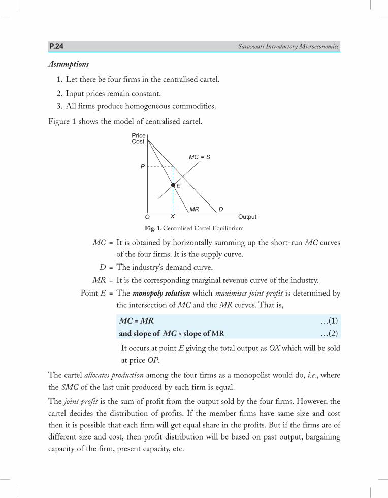
Saraswati Introductory MicroeconomicsP.24
Assumptions
1. Let there be four firms in the centralised cartel.
2. Input prices remain constant.
3. All firms produce homogeneous commodities.
Figure 1 shows the model of centralised cartel.
OutputODMR
P
X
E
PriceCost
MC = S
Fig. 1. Centralised Cartel Equilibrium
MC = It is obtained by horizontally summing up the short-run MC curves of the four firms. It is the supply curve.
D = The industry’s demand curve.
MR = It is the corresponding marginal revenue curve of the industry.
Point E = The monopoly solution which maximises joint profit is determined by the intersection of MC and the MR curves. That is,
MC = MR …(1)
and slope of MC > slope of MR …(2)
It occurs at point E giving the total output as OX which will be sold at price OP.
The cartel allocates production among the four firms as a monopolist would do, i.e., where the SMC of the last unit produced by each firm is equal.
The joint profit is the sum of profit from the output sold by the four firms. However, the cartel decides the distribution of profits. If the member firms have same size and cost then it is possible that each firm will get equal share in the profits. But if the firms are of different size and cost, then profit distribution will be based on past output, bargaining capacity of the firm, present capacity, etc.
Cartels P.25
ConclusionIn reality, cartels can rarely achieve maximum joint profits. William Fellner gives the following reasons why industry’s profits may not be maximised:
1. Mistakes in the estimation of market demand
Each firm believes that elasticity of its demand curve is high due to the existence of perfect substitutes and that of the industry’s demand is less. The result is that worng estimation of market demand leads to mistakes in the estimation of the MR and hence, in the estimation of price.
2. Mistakes in the estimation of marginal cost
There are mistakes in the estimation of MC due to lack of adequate and correct cost data.
3. Slow process of cartel negotiations
Cartel negotiations take a long time due to differences in size, cost and market of the individual firms. By the time an agreement is reached, it renders the initial estimate obsolete.
4. ‘Rigidity’ of the negotiated price
Due to the long time taken by cartel negotiations, once the agreement about price is reached it remains rigid over periods.
5. The ‘bluffing’ attitude of some members
Bluffing attitude during the bargaining process leads to miscalculation of the real equilibrium price and output.
6. Desire to build a good public image
It will force the members of the cartel to charge a ‘fair price’ and no the profit-maximising price.
7. Fear of entry
Large profit will attract new firms. The established members/firms prefer to charge a lower price to prevent entry, as they fear that new entrants will wipe away profit.
Objective: To study why different prices are charged for the same commodity.
The Concept
Price discrimination is the practice of charging different prices from different consumers for the same good or service at the same time. When the monopoly firm practices price discrimination, it is called discriminating monopoly. The other words for price discrimination are ‘selective pricing’ or ‘pricing by market segmentation’ or ‘charging what the traffic will bear’. The cost of production is either the same or it differs by a small margin. Products are basically the same but the producers convince the consumers that the products are different on the basis of different brand name, different packaging, different advertising, etc. We will deal with identical products, produced under same cost and sold at different prices to different consumers.
Conditions for Price Discrimination
The conditions which are essential for the implementation of price discrimination are:
1. There should be monopoly or other forms of imperfect competition present in the market. Price discrimination cannot be implemented under perfect competition.
2. There should be two or more markets which can be separated and can be kept separate. If they cannot be kept separate then the consumer can resell the monopoly product in the high priced market.
3. The elasticity of demand in these two or more markets must be different. If coefficient of price elasticity of demand is same in all markets, then price discrimination cannot be implemented.
4. There should be no contact among buyers. 5. The monopolist must have complete control over the supply of the commodity.
Degrees of Types of Price Discrimination
A.C. Pigou has differentiated between three forms of price discrimination. These are:
First Degree Price Discrimination
In the first degree, the monopolist behaves as if he sold each unit of the commodity separately to consumers and charged the maximum price he could obtain for each unit. By practicing first degree, the monopolist is able to extract from consumers all of the consumer surplus, i.e., consumer surplus is zero. The discriminating monopolist, in first degree, Negotiates individually with each consumer and charges the maximum price he is willing to pay. This is ‘take-it-or-leave-it’ price discrimination and is, therefore, called perfect price discrimination.
Project-9: Price Discrimination
Price discrimination P.27
First degree is rare in the real world. If a monopolist wants to practice it, he must have exact knowledge of the demand curve facing his product and charge exactly the same amount the consumer is willing to pay.
Second Degree Price DiscriminationIn the second degree, the discriminating monopolist sets a uniform price per unit for specific quantity of a commodity, a lower price per unit for a specific additional quantity of the commodity and so on. In this case, the discriminating monopolist is able to extract a large part of the consumer surplus. Second degree is also called non-linear pricing. Second degree is fairly common in the real world. Public utilities like electricity supply and telephone company practice second degree.
Third Degree Price DiscriminationThird degree price discrimination occurs when the monopolist charges different prices for the same commodity in different markets or groups. To practice third degree price discrimination, the monopolist must be able to separate markets or groups and charge them different prices depending upon their coefficient of price elasticity of demand. In the third degree, the monopolist is able to extract a large part of consumer surplus.Third degree is a normal form of price discriminations which is fairly common. For example, electric power companies charge higher rates from industrial and commercial users and lower rates from residential areas. The markets are kept separated by different meters.Another example is dumping. A nation behaves like a monopolist in its own home market but the demand curve for the monopolist’s product in the foreign market is perfectly elastic as substitutes are available from other nations.Other examples are discounts for a particular group of people like the bus transport pass for students, senior citizen’s discount, army personnel’s discount, etc.The effects of price discrimination are:
1. The discriminating monopolist is able to extract a large part of consumer surplus. 2. The discriminating monopolist’s total revenue and total profit will be more. 3. Output sold in the market will increase.
Conclusion
Bad Effects of Price DiscriminationPrice discrimination is not desirable on the following grounds:
1. Problem of economic allocation of resources Price discrimination leads to destruction of competition from rival firms and
strengthening of its own power and hence, inefficient and uneconomic allocation of resources.
Saraswati Introductory MicroeconomicsP.28
2. Maldistribution of goods between consumers Price discrimination causes discontent and dissatisfaction among those rich consumers
who have to pay higher prices and those poor consumers who have to do without the good because they do not have the required money to buy it.
3. Dumping In case of dumping, higher price is charged in the home market and a lower price in
the world market.
Good Effects of Price DiscriminationPrice discrimination is desirable on the following grounds:
1. It promotes equity
When price is raised for the rich section of the society and lowered for the poor section, it has a redistributive effect. It reduces the inequalities of income. The poor people can have access to certain essential goods and services, like those of a doctor.
2. It makes production feasible
Certain commodities can be profitably produced only under discriminating monopoly. Price discrimination helps to produce those goods which pure monopolist will not produce.
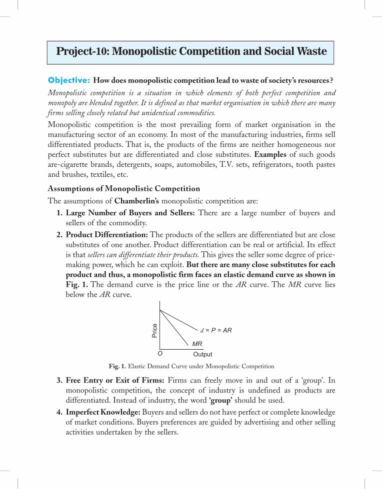
Objective: How does monopolistic competition lead to waste of society’s resources ?
Monopolistic competition is a situation in which elements of both perfect competition and monopoly are blended together. It is defined as that market organisation in which there are many firms selling closely related but unidentical commodities.
Monopolistic competition is the most prevailing form of market organisation in the manufacturing sector of an economy. In most of the manufacturing industries, firms sell differentiated products. That is, the products of the firms are neither homogeneous nor perfect substitutes but are differentiated and close substitutes. Examples of such goods are-cigarette brands, detergents, soaps, automobiles, T.V. sets, refrigerators, tooth pastes and brushes, textiles, etc.
Assumptions of Monopolistic Competition
The assumptions of Chamberlin’s monopolistic competition are: 1. Large Number of Buyers and Sellers: There are a large number of buyers and
sellers of the commodity. 2. Product Differentiation: The products of the sellers are differentiated but are close
substitutes of one another. Product differentiation can be real or artificial. Its effect is that sellers can differentiate their products. This gives the seller some degree of price-making power, which he can exploit. But there are many close substitutes for each product and thus, a monopolistic firm faces an elastic demand curve as shown in Fig. 1. The demand curve is the price line or the AR curve. The MR curve lies below the AR curve.
MR
d = P = AR
OutputO
Pric
e
Fig. 1. Elastic Demand Curve under Monopolistic Competition
3. Free Entry or Exit of Firms: Firms can freely move in and out of a ‘group’. In monopolistic competition, the concept of industry is undefined as products are differentiated. Instead of industry, the word ‘group’ should be used.
4. Imperfect Knowledge: Buyers and sellers do not have perfect or complete knowledge of market conditions. Buyers preferences are guided by advertising and other selling activities undertaken by the sellers.
Project-10: Monopolistic Competition and Social Waste
Saraswati Introductory MicroeconomicsP.30
5. Selling Cost: A firm under monopolistic competition incus selling cost which is the cost of promoting the demand for its product. Example of selling costs are advertisements, window displays, salesman’s salaries, etc. The most important form of selling cost in advertising. Advertising can be of three kinds: informative, persuasive and defensive. Informative advertising gives information about new product’s price, quality, location, supply, etc. It makes market function more effectively. It is a low cost method. Some examples of informative advertising are yellow pages, newspapers and magazines. Persuasive advertising attempts to persuade consumers of the desirability of the product. The information given about the product may or may not be correct. Defensive advertising is undertaken only when the rivals are advertising. It leads to more cost for all firms. It is a wasteful expenditure.
6. High Transportation Cost: Cost of transporting the commodity from one place to another place is very high under monopolistic competition.
Product Differentiation and the Demand CurveProduct differentiation means a consumer can distinguish between the product of one producer from that of the other producer. It means that due to some difference in the products, they create a different impression in the mind of the consumer. Product differentiation can be of two types: 1. Real Product Differentiation It occurs when the inherent characteristics of the products are different. Difference
in smell, taste and/or quality of inputs are some ways of bringing about real product differentiation.
2. Artificial Product Differentiation It occurs when the products are basically the same yet the consumer is persuaded,
via advertising, good salesmanship, packaging and other selling activities, that the products are different. It is also called fancied product differentiation. Difference in design, shape, size, brand name and/or packaging are some ways of bringing about artificial product differentiation. It can also be the result of the individual’s personal assessment of the good or service. The result is that consumers are willing to pay different prices for what is actually the same product.
The effect of product differentiation is that sellers can differentiate their product and this brings in the monopoly element in monopolistic competition. Each seller has some degree of monopoly power which he can exploit. He acts as a price-searcher or maker and not as a price-taker. However, because there are many close substitutes of the product, the discretion over the determination of price is limited.
Product differentiation creates brand loyalty of the consumer and gives rise to a negatively sloping demand curve.
Monopolistic Competition and Social Waste P.31
Conclusion
Social Waste Under Monopolistic Competition are:
1. Unemployment
In monopolistic competition, resources are not fully exploited. The plant capacity remains under-utilised. It results in under-employment of resources. There is more emphasis on regulation of prices. It leads to either over-production under-production. The recurrence of business fluctuations renders the factors of production jobless.
2. Excessive Cross Transport Cost
Unnecessary expenditure on the transportation of goods to far flung areas is a waste. It would be much better if a single firm serves a particular area.
3. Lack of Specialisation
Producers under monopolistic competition do not produce a single good. Many goods are produced to minimise the risks and uncertainties of business. As a result, there is lack of specialisation which raises the cost of production.
4. Excessive Expenditure on Advertisement
If selling cost is incurred to educate the customers about the existence of a particular product in the market, it is considered good. But producers spend huge amount of money on publicity just to attract the buyers towards their products.
5. Excess Capacity
A firm does not produce at its full capacity in the long run. The downward sloping demand curve of the firm does not touch the average cost curve at its minimum point. As a result, equilibrium level of the output is low and the price is high. The unused capacity of the firms is a social waste.
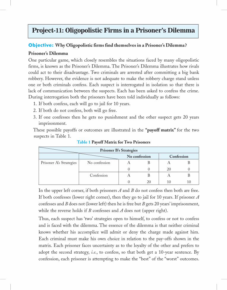
Objective: Why Oligopolistic firms find themselves in a Prisoner’s Dilemma?
Prisoner’s DilemmaOne particular game, which closely resembles the situations faced by many oligopolistic firms, is known as the Prisoner’s Dilemma. The Prisoner’s Dilemma illustrates how rivals could act to their disadvantage. Two criminals are arrested after committing a big bank robbery. However, the evidence is not adequate to make the robbery charge stand unless one or both criminals confess. Each suspect is interrogated in isolation so that there is lack of communication between the suspects. Each has been asked to confess the crime. During interrogation both the prisoners have been told individually as follows: 1. If both confess, each will go to jail for 10 years. 2. If both do not confess, both will go free. 3. If one confesses then he gets no punishment and the other suspect gets 20 years
imprisonment. These possible payoffs or outcomes are illustrated in the “payoff matrix” for the two suspects in Table 1.
Table 1 Payoff Matrix for Two Prisoners
Prisoner B’s Strategies
No confession Confession
Prisoner A’s Strategies No confession A
0
B
0
A
20
B
0
Confession A
0
B
20
A
10
B
10
In the upper left corner, if both prisoners A and B do not confess then both are free. If both confesses (lower right corner), then they go to jail for 10 years. If prisoner A confesses and B does not (lower left) then he is free but B gets 20 years’ imprisonment, while the reverse holds if B confesses and A does not (upper right).
Thus, each suspect has ‘two’ strategies open to himself, to confess or not to confess and is faced with the dilemma. The essence of the dilemma is that neither criminal knows whether his accomplice will admit or deny the charge made against him. Each criminal must make his own choice in relation to the pay-offs shown in the matrix. Each prisoner faces uncertainty as to the loyalty of the other and prefers to adopt the second strategy, i.e., to confess, so that both get a 10-year sentence. By confession, each prisoner is attempting to make the “best” of the “worst” outcomes.
Project-11: Oligopolistic Firms in a Prisoner’s Dilemma
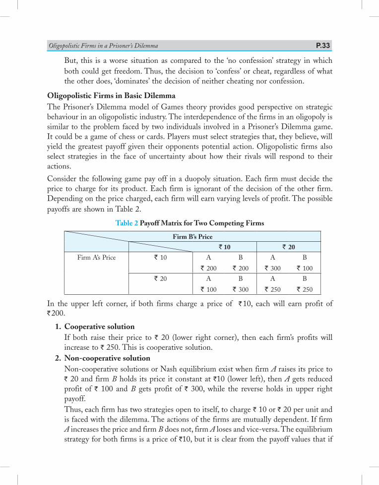
Oligopolistic Firms in a Prisoner’s Dilemma P.33
But, this is a worse situation as compared to the ‘no confession’ strategy in which both could get freedom. Thus, the decision to ‘confess’ or cheat, regardless of what the other does, ‘dominates’ the decision of neither cheating nor confession.
Oligopolistic Firms in Basic DilemmaThe Prisoner’s Dilemma model of Games theory provides good perspective on strategic behaviour in an oligopolistic industry. The interdependence of the firms in an oligopoly is similar to the problem faced by two individuals involved in a Prisoner’s Dilemma game. It could be a game of chess or cards. Players must select strategies that, they believe, will yield the greatest payoff given their opponents potential action. Oligopolistic firms also select strategies in the face of uncertainty about how their rivals will respond to their actions.
Consider the following game pay off in a duopoly situation. Each firm must decide the price to charge for its product. Each firm is ignorant of the decision of the other firm. Depending on the price charged, each firm will earn varying levels of profit. The possible payoffs are shown in Table 2.
Table 2 Payoff Matrix for Two Competing Firms
Firm B’s Price
` 10 ` 20
Firm A’s Price ` 10 A
` 200
B
` 200
A
` 300
B
` 100
` 20 A
` 100
B
` 300
A
` 250
B
` 250
In the upper left corner, if both firms charge a price of ` 10, each will earn profit of ` 200.
1. Cooperative solution If both raise their price to ` 20 (lower right corner), then each firm’s profits will
increase to ` 250. This is cooperative solution. 2. Non-cooperative solution Non-cooperative solutions or Nash equilibrium exist when firm A raises its price to
` 20 and firm B holds its price it constant at `10 (lower left), then A gets reduced profit of ` 100 and B gets profit of ` 300, while the reverse holds in upper right payoff.
Thus, each firm has two strategies open to itself, to charge ` 10 or ` 20 per unit and is faced with the dilemma. The actions of the firms are mutually dependent. If firm A increases the price and firm B does not, firm A loses and vice-versa. The equilibrium strategy for both firms is a price of `10, but it is clear from the payoff values that if
Saraswati Introductory MicroeconomicsP.34
they could communicate and reach an effective agreement to charge ` 15, they would earn higher profits of ` 250 each. This type of situation is known as the Prisoner’s Dilemma.
ConclusionA good deal of experiments have been done on the testing of Prisoner’s Dilemma hypothesis in oligopoly theory. These empirical tests were done by L.B. Lave, Dolbear, J.L, Murphy, Fouraker Siegel, and J.W. Friedman.
The evidence forthcoming from the above empirical studies conclude that: 1. Joint profitability can be materially improved through collusion or co-operation, and 2. The attitude of firms towards collusion would be coloured by past experience of
price-wars and the degree of uncertainty which they face.
Furthermore, the extent of collusion can be said to depend upon: 1. The number of firms within the industry. Greater the number of firms, harder it
becomes to detect secret price cutting. 2. The amount of information possessed by each firm about its rivals. 3. Strategic Behaviour: When each firm operates in the market strategically, Nash
equilibrium is attained. In the words of Lipsey and Chrystal. “If a Nash equilibrium is established-by any means whatsoever-no firm has an incentive to depart from it by altering its own behaviour. It is self policing”. The basis of Nash equilibrium is rational decision making in the absence of cooperation.
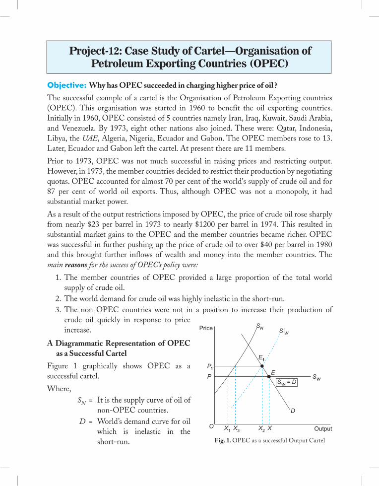
Objective: Why has OPEC succeeded in charging higher price of oil ?
The successful example of a cartel is the Organisation of Petroleum Exporting countries (OPEC). This organisation was started in 1960 to benefit the oil exporting countries. Initially in 1960, OPEC consisted of 5 countries namely Iran, Iraq, Kuwait, Saudi Arabia, and Venezuela. By 1973, eight other nations also joined. These were: Qatar, Indonesia, Libya, the UAE, Algeria, Nigeria, Ecuador and Gabon. The OPEC members rose to 13. Later, Ecuador and Gabon left the cartel. At present there are 11 members.
Prior to 1973, OPEC was not much successful in raising prices and restricting output. However, in 1973, the member countries decided to restrict their production by negotiating quotas. OPEC accounted for almost 70 per cent of the world's supply of crude oil and for 87 per cent of world oil exports. Thus, although OPEC was not a monopoly, it had substantial market power.
As a result of the output restrictions imposed by OPEC, the price of crude oil rose sharply from nearly $23 per barrel in 1973 to nearly $1200 per barrel in 1974. This resulted in substantial market gains to the OPEC and the member countries became richer. OPEC was successful in further pushing up the price of crude oil to over $40 per barrel in 1980 and this brought further inflows of wealth and money into the member countries. The main reasons for the success of OPEC's policy were:
1. The member countries of OPEC provided a large proportion of the total world supply of crude oil.
2. The world demand for crude oil was highly inelastic in the short-run. 3. The non-OPEC countries were not in a position to increase their production of
crude oil quickly in response to price increase.
A Diagrammatic Representation of OPEC as a Successful Cartel
Figure 1 graphically shows OPEC as a successful cartel.
Where, SN = It is the supply curve of oil of
non-OPEC countries. D = World’s demand curve for oil
which is inelastic in the short-run.
Project-12: Case Study of Cartel—Organisation of Petroleum Exporting Countries (OPEC)
O
P1
E1
PE
X1 X2X3 X
D
Price
Output
SW
S'WSN
SW = D
Fig. 1. OPEC as a successful Output Cartel
Saraswati Introductory MicroeconomicsP.36
OP = Initially the OPEC countries are willing to supply all crude oil that is demanded at the world price OP. Therefore, the world supply curve for crude oil is the horizontal curve, SW .
Point E = The world’s supply curve (SW) cuts the world’s demand curve for oil, (D) at point E. Thus, OX is the total output of oil produced. Out of OX, OX1 is supplied by non-OPEC countries and X1X by the OPEC countries.
S'W = By fixing its production quota, OPEC shifted the world supply curve to S'W . The horizontal distance between SN and S'W curves is OPEC’s production.
Point E1 = The new world’s supply curves S'W intersects the world's demand curve at point E1. Thus, world price increased to P1 and output reduced of OX2. At price OP1, the non-OPEC countries supply OX3 units and OPEC country supply X3 X2 units.
Result : OPEC was able to increase its oil revenue because although sales declined price rose more than in proportion. Non-OPEC countries also benefited due to rise in price.
Pressure on the Cartel
In the long period, cartel started feeling the pressure due to the following three reasons:
1. Increasing world supply 2. Declining world demand 3. The pressure to cheat
1. Increasing world supply
Since OPEC countries had high prices and high profits, the non-OPEC producers made considerable attempts to find additional sources of oil to enlarge their production capacity. As a result, the overall share of OPEC cartel in world crude oil supply fell drastically from more than 70 per cent in 1973 to less than 40 per cent in 1988. This increased supply of oil by non-OPEC countries tended to drive the world price down and weakened the power of OPEC.
2. Declining world demand
While in the short-run, the demand for crude oil proved to be highly inelastic, in the long-run user countries to economise on the use of oil by having technological substitutes like fuel efficient small cars, more economical diesel engines, more efficient insulation on oil-heated buildings, etc. and a search for alternatives to petroleum like solar power, wind power, etc. As a result, the long-run demand curve for crude oil turned out to be much more elastic than the short-run demand curve. Therefore, to maintain high prices, OPEC had to cut down production levels.
Case Study of Cartel—Organisation of Petroleum Exporting Countries (OPEC) P.37
3. Pressure to cheat
The pressure on OPEC members to cut down production levels in order to maintain high prices led to serious differences among the member countries. OPEC was unable to prevent a fall in crude oil prices. There was widespread cheating among the menber countries.
Conclusion
The experience of OPEC cartel brings out the following basics difficulties of the output restricting schemes:
1. Where demand is inelastic, restriction of output to below the competitive level can lead to immense profits in the short-run. However, in the long run, new producers appear, demand falls and substitutes are invented and produced. This reduces the power of the cartel in the long-run.
2. Maintaining market power becomes increasingly difficult as time passes. 3. Producers with market power face a basic trade-off between profits in the short-term
and profits in the longer term. 4. Output restriction by voluntary agreement among several producers is difficult to
maintain over long period of time.
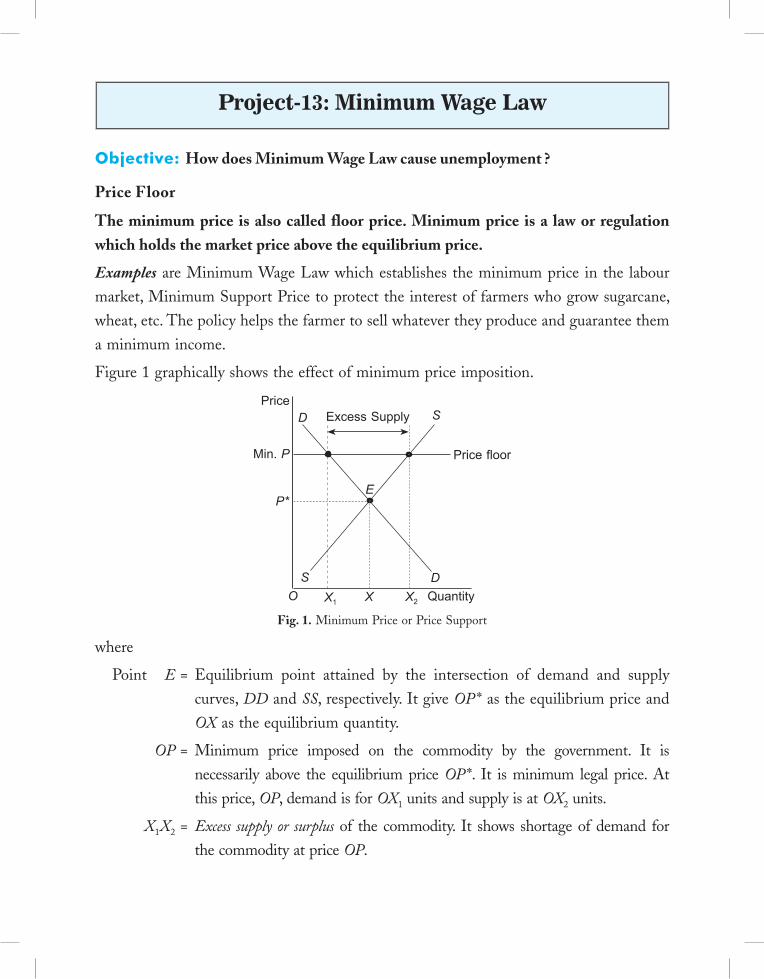
Objective: How does Minimum Wage Law cause unemployment ?
Price Floor
The minimum price is also called floor price. Minimum price is a law or regulation which holds the market price above the equilibrium price.
Examples are Minimum Wage Law which establishes the minimum price in the labour market, Minimum Support Price to protect the interest of farmers who grow sugarcane, wheat, etc. The policy helps the farmer to sell whatever they produce and guarantee them a minimum income.
Figure 1 graphically shows the effect of minimum price imposition.
Excess Supply
X2O XD
P*E
PriceS
Min. P
X1
D
Price floor
SQuantity
Fig. 1. Minimum Price or Price Support
where
Point E = Equilibrium point attained by the intersection of demand and supply curves, DD and SS, respectively. It give OP * as the equilibrium price and OX as the equilibrium quantity.
OP = Minimum price imposed on the commodity by the government. It is necessarily above the equilibrium price OP *. It is minimum legal price. At this price, OP, demand is for OX1 units and supply is at OX2 units.
X1X2 = Excess supply or surplus of the commodity. It shows shortage of demand for the commodity at price OP.
Project-13: Minimum Wage Law
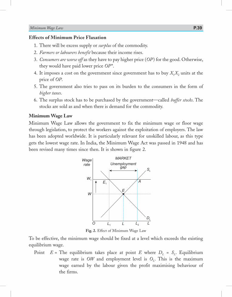
Minimum Wage Law P.39
Effects of Minimum Price Flaxation
1. There will be excess supply or surplus of the commodity. 2. Farmers or labourers benefit because their income rises. 3. Consumers are worse off as they have to pay higher price (OP ) for the good. Otherwise,
they would have paid lower price OP *. 4. It imposes a cost on the government since government has to buy X1X2 units at the
price of OP. 5. The government also tries to pass on its burden to the consumers in the form of
higher taxes. 6. The surplus stock has to be purchased by the government—called buffer stocks. The
stocks are sold as and when there is demand for the commodity.
Minimum Wage LawMinimum Wage Law allows the government to fix the minimum wage or floor wage through legislation, to protect the workers against the exploitation of employers. The law has been adopted worldwide. It is particularly relevant for unskilled labour, as this type gets the lowest wage rate. In India, the Minimum Wage Act was passed in 1948 and has been revised many times since then. It is shown in figure 2.
MarkEtUnemployment
gap
L2
E1
O LDL
W
a
E
Wagerate
SL
W1
L1 L
Fig. 2. Effect of Minimum Wage Law
To be effective, the minimum wage should be fixed at a level which exceeds the existing equilibrium wage.
Point E = The equilibrium takes place at point E where DL = SL. Equilibrium wage rate is OW and employment level is OL. This is the maximum wage earned by the labour given the profit maximising behaviour of the firms.
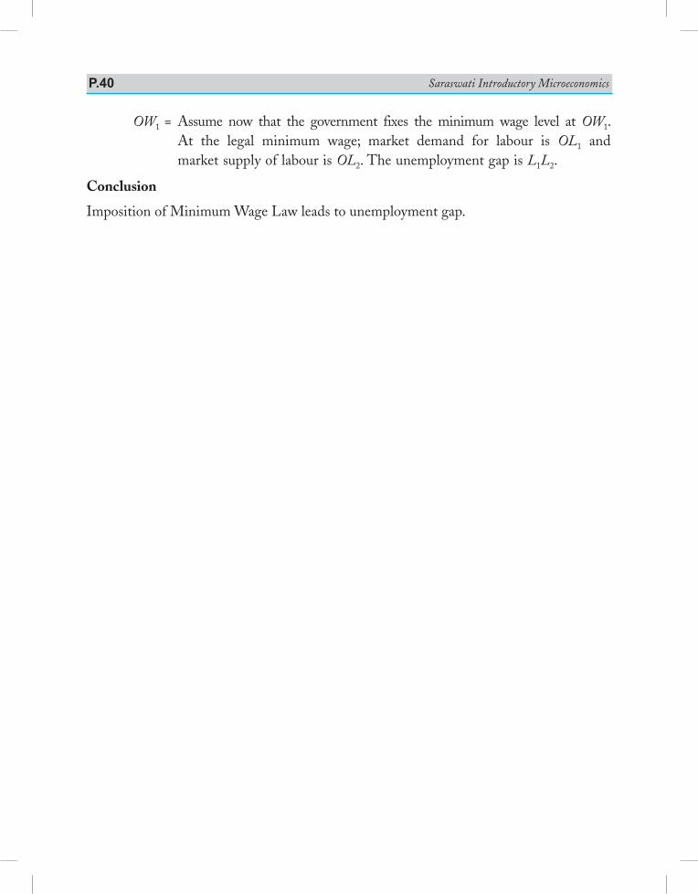
Saraswati Introductory MicroeconomicsP.40
OW1 = Assume now that the government fixes the minimum wage level at OW1. At the legal minimum wage; market demand for labour is OL1 and market supply of labour is OL2. The unemployment gap is L1L2.
Conclusion
Imposition of Minimum Wage Law leads to unemployment gap.
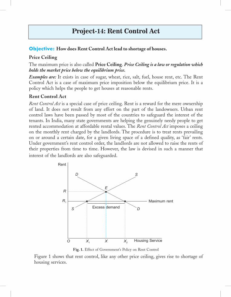
Objective: How does Rent Control Act lead to shortage of houses.
Price CeilingThe maximum price is also called Price Ceiling. Price Ceiling is a law or regulation which holds the market price below the equilibrium price.Examples are: It exists in case of sugar, wheat, rice, salt, fuel, house rent, etc. The Rent Control Act is a case of maximum price imposition below the equilibrium price. It is a policy which helps the people to get houses at reasonable rents.
Rent Control ActRent Control Act is a special case of price ceiling. Rent is a reward for the mere ownership of land. It does not result from any effort on the part of the landowners. Urban rent control laws have been passed by most of the countries to safeguard the interest of the tenants. In India, many state governments are helping the genuinely needy people to get rented accommodation at affordable rental values. The Rent Control Act imposes a ceiling on the monthly rent charged by the landlords. The procedure is to treat rents prevailing on or around a certain date, for a given living space of a defined quality, as ‘fair’ rents. Under government’s rent control order, the landlords are not allowed to raise the rents of their properties from time to time. However, the law is devised in such a manner that interest of the landlords are also safeguarded.
Excess demandMaximum rent
Housing Service
D
R1
R
X1O
D S
E
Rent
X X2
S
Fig. 1. Effect of Government’s Policy on Rent Control
Figure 1 shows that rent control, like any other price ceiling, gives rise to shortage of housing services.
Project-14: Rent Control Act
Saraswati Introductory MicroeconomicsP.42
In the figure, DD = Demand curve for housing services SS = Supply curve of housing services In the initial situation, when rent ceiling is not imposed the demand and supply curves
of the housing services (DD and SS) intersect at point E. The equilibrium level of housing services is OX and the rent is OR. The shortage will be more, higher the elasticities of demand and supply.
If the government implements its policy to control the rent by imposing a ceiling on rent, say, at the level OR1, then the result is an excess demand for housing services to the extent of X1 X2. That is, the landlords are willing to supply only X1 units of housing services and the tenants are demanding X2 units at rent OR1.
ConclusionEffects of Rent Control Act are as follows: 1. Poor Quality and Less Supply: The effect of rent control is that since owners of
rental units receive lower rent, they do not have the incentive to maintain and rent housing services. Initially, when the policy is implemented, interest of owners is harmed as they get lower returns by law. The law intends to benefit the tenants. It is debatable if tenants actually benefit from rent control. Though tenants get houses at lower rents; lower rent does not ensure the availability of houses. Moreover, there is fall in the quality of rental housing which eliminates the benefit of lower rents to the tenants.
2. Non-Price Rationing of Rental Units: Since demand is more than supply, the owners may start pursuing non-price rationing of rental units. For example, conditions may be imposed on potential tenants like not allowing cooking of non-vegetarian food, not allowing tenants to keep pets, etc. If owners could charge the market rent, such conditions may not be imposed.
3. Black Market Will Emerge: The landlords will demand huge amount of security. The tenants who will refuse to pay, will not be given the accommodation.
4. Fall in Revenue to the Governments: Rent Control Act reduces the market price of rental units. Thus, the amount of property tax collected by the government falls.
5. Short-Run Effects of the Act: The beneficial effect of this Act are felt by the tenants only in the short-run. In the short-run, supply curve of houses is inelastic. That is, both quality and quantity of houses cannot change in the short run. So, the tenants enjoy good quality houses at lower rents.
6. Long-Run Effect of Act: In the long-run, the supply curve of houses is elastic landlords will reduce supply of housing services on one hand and will reduce maintenance of the existing units on the other hand.
Objective: To apply the concept of elasticity of demand on Newspaper.
Example of British NewspapersSituation: Five main British newspapers are—The Times, The Guardian, The Daily Telegraph, The Financial Times and The Independent. Generally, it has been noticed that: — Newspapers have low income elasticity. — Newspapers have low price elasticity of demand. — People do not change their newspaper frequently. — If cross elasticity between two newspapers is high then they are good substitutes
of each other. Cross elasticity of demand between The Times and The Independent was + 0.42.
— Each newspaper has a stable market.
But in September 1993, the owners of The Times newspaper lowered its price by one-third.Effect: The effects of fall in price by The Times were as follows: (a) Initially the rival newspapers did not follow the price cut. It led to their declining
sales as they lost their reader to The Times. (b) The Independent, a close substitute of The Times, suffered most (14% loss of sales).
The demand curve of The Independent shifted to the left. (c) The Time’s daily sales revenues fell because the newspaper had inelastic demand
(–0.57). As price fell, quantity demanded increased but the increase was not in a greater proportion.
(d) The Times recovered its loss by raising advertising rates as the newspaper had more circulation (or readers).
(e) Since The Independent was in financial difficulty, it was taken over by the Mirror Group who was financially stronger. Later, the Mirror Group sold The Independent to an Irish newspaper group.
(f) The Independent and other newspaper reacted to The Times growing market share by cutting their price.
The example shows how in a real life situation decision taken by rival firms are affected by different kinds of elasticity of demand.
ConclusionA situation of price war began. The Times further reduced its price.
Project-15: Elasticity of Demand—Case Study of Newspaper
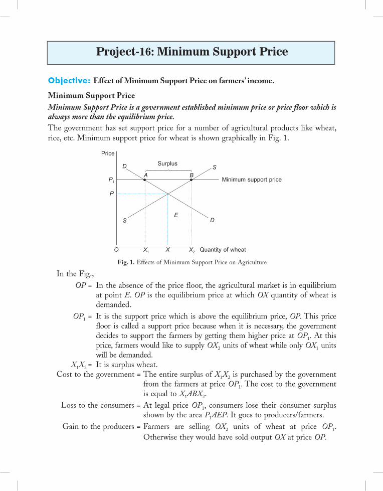
Objective: Effect of Minimum Support Price on farmers’ income.
Minimum Support PriceMinimum Support Price is a government established minimum price or price floor which is always more than the equilibrium price.The government has set support price for a number of agricultural products like wheat, rice, etc. Minimum support price for wheat is shown graphically in Fig. 1.
P1
P
Surplus
Minimum support price
Quantity of wheatX2XX1O
S D
D SA
Price
B
Fig. 1. Effects of Minimum Support Price on Agriculture
In the Fig., OP = In the absence of the price floor, the agricultural market is in equilibrium
at point E. OP is the equilibrium price at which OX quantity of wheat is demanded.
OP1 = It is the support price which is above the equilibrium price, OP. This price floor is called a support price because when it is necessary, the government decides to support the farmers by getting them higher price at OP1. At this price, farmers would like to supply OX2 units of wheat while only OX1 units will be demanded.
X1X2 = It is surplus wheat. Cost to the government = The entire surplus of X1X2 is purchased by the government
from the farmers at price OP1. The cost to the government is equal to X1ABX2.
Loss to the consumers = At legal price OP1, consumers lose their consumer surplus shown by the area P1AEP. It goes to producers/farmers.
Gain to the producers = Farmers are selling OX2 units of wheat at price OP1. Otherwise they would have sold output OX at price OP.
Project-16: Minimum Support Price
E
Minimum Support Price P.45
Effect of Minimum Support Price
The effects are:
1. Farmers benefit because they receive higher price for their product.
2. Farmer’s income rises. Earlier (in equilibrium), the income was OPEX. After the minimum support price the income has risen to OP1BX2.
3. Consumers are worse off because they have to pay higher price (OP1) for when under the support price scheme. Loss in consumer surplus = P1AEP.
4. Consumers have to pay higher tax to provide funds to the government for the purchase of surplus wheat.
5. The policy imposes a cost to the government equal to X1ABX2.
6. The Food Corporation of India (FCI) procures surplus wheat and rice on behalf of the government. The grain is stored in its warehouses. The government incurs heavy losses as it has to subsidise the consumption of these grains through public distribution system (PDS).
ConclusionHence, the policy of minimum support price leads to welfare loss to the society. If the government wants to provide income support to those farmers who are financially distressed and do not have sufficient income to finance their indebtedness, it is better to stabilise their income directly.
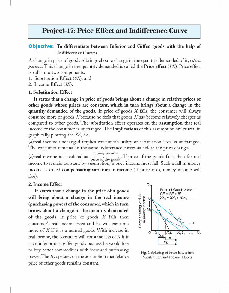
Objective: To differentiate between Inferior and Giffen goods with the help of Indifference Curves.
A change in price of goods X brings about a change in the quantity demanded of it, ceteris paribus. This change in the quantity demanded is called the Price effect (PE). Price effect is split into two components:1. Substitution Effect (SE), and2. Income Effect (IE).
1. Substitution Effect It states that a change in price of goods brings about a change in relative prices of other goods whose prices are constant, which in turn brings about a change in the quantity demanded of the goods. If price of goods X falls, the consumer will always consume more of goods X because he feels that goods X has become relatively cheaper as compared to other goods. The substitution effect operates on the assumption that real income of the consumer is unchanged. The implications of this assumption are crucial in graphically plotting the SE, i.e.,(a) real income unchanged implies consumer’s utility or satisfaction level is unchanged. The consumer remains on the same indifference curves as before the price change.
(b) real income is calculated as money income
price of the goods. If price of the goods falls, then for real
income to remain constant by assumption, money income must fall. Such a fall in money income is called compensating variation in income (If price rises, money income will rise).
2. Income Effect It states that a change in the price of a goods will bring about a change in the real income (purchasing power) of the consumer, which in turn brings about a change in the quantity demanded of the goods. If price of goods X falls then consumer’s real income rises and he will consume more of X if it is a normal goods. With increase in real income, the consumer will consume less of X if it is an inferior or a giffen goods because he would like to buy better commodities with increased purchasing power. The IE operates on the assumption that relative price of other goods remains constant.
Fig. 1 Splitting of Price Effect into Substitution and Income Effects
Price of Good fallsX
PE SE IE= +XX = XX + X X2 1 1 2
Co
mp
en
sa
ting
va
ria
tion
inm
on
ey
incom
e
QY
M
M1
O XSE
IE
PE
QXL2L1X2X L1
e1 e2
I2I1
e
Project-17: Price Effect and Indifference Curve
s X falls
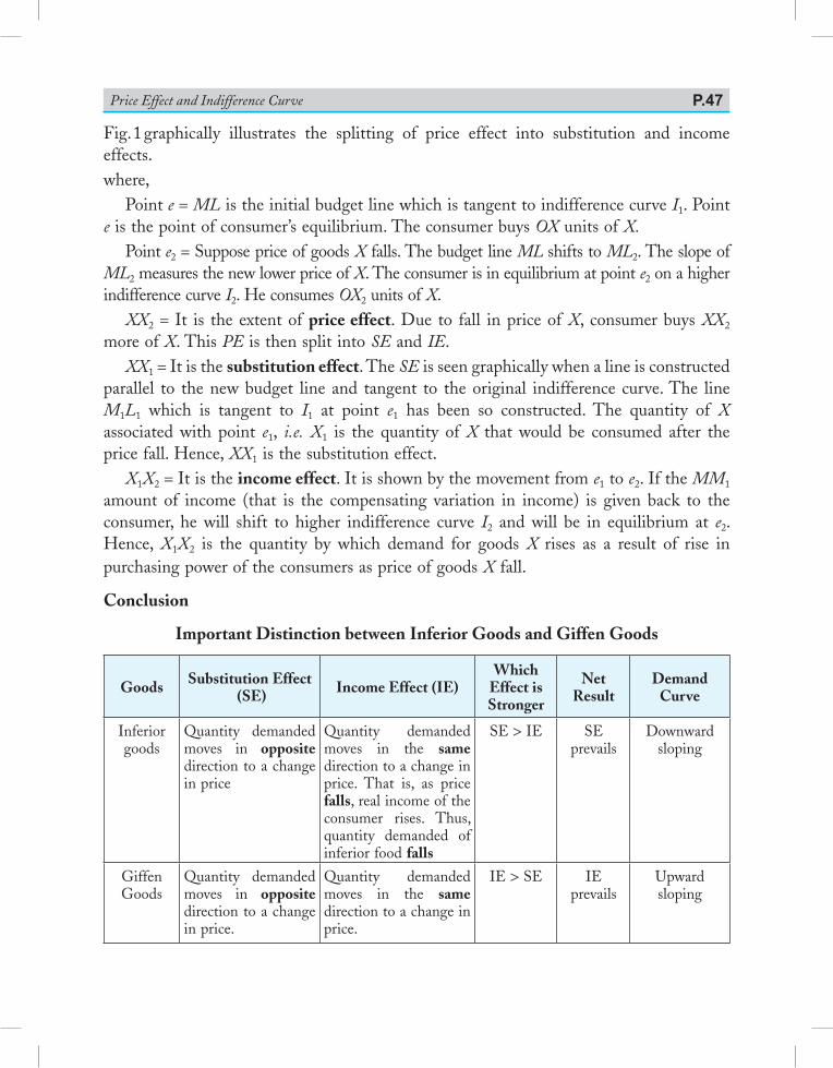
Price Effect and Indifference Curve P.47
Fig. 1 graphically illustrates the splitting of price effect into substitution and income effects.where, Point e = ML is the initial budget line which is tangent to indifference curve I1. Point e is the point of consumer’s equilibrium. The consumer buys OX units of X. Point e2 = Suppose price of goods X falls. The budget line ML shifts to ML2. The slope of ML2 measures the new lower price of X. The consumer is in equilibrium at point e2 on a higher indifference curve I2. He consumes OX2 units of X. XX2 = It is the extent of price effect. Due to fall in price of X, consumer buys XX2 more of X. This PE is then split into SE and IE. XX1 = It is the substitution effect. The SE is seen graphically when a line is constructed parallel to the new budget line and tangent to the original indifference curve. The line M1L1 which is tangent to I1 at point e1 has been so constructed. The quantity of X associated with point e1, i.e. X1 is the quantity of X that would be consumed after the price fall. Hence, XX1 is the substitution effect. X1X2 = It is the income effect. It is shown by the movement from e1 to e2. If the MM1 amount of income (that is the compensating variation in income) is given back to the consumer, he will shift to higher indifference curve I2 and will be in equilibrium at e2. Hence, X1X2 is the quantity by which demand for goods X rises as a result of rise in purchasing power of the consumers as price of goods X fall.
Conclusion
Important Distinction between Inferior Goods and Giffen Goods
Goods Substitution Effect (SE) Income Effect (IE)
Which Effect is Stronger
Net Result
Demand Curve
Inferior goods
Quantity demanded moves in opposite direction to a change in price
Quantity demanded moves in the same direction to a change in price. That is, as price falls, real income of the consumer rises. Thus, quantity demanded of inferior food falls
SE > IE SE prevails
Downward sloping
Giffen Goods
Quantity demanded moves in opposite direction to a change in price.
Quantity demanded moves in the same direction to a change in price.
IE > SE IE prevails
Upward sloping
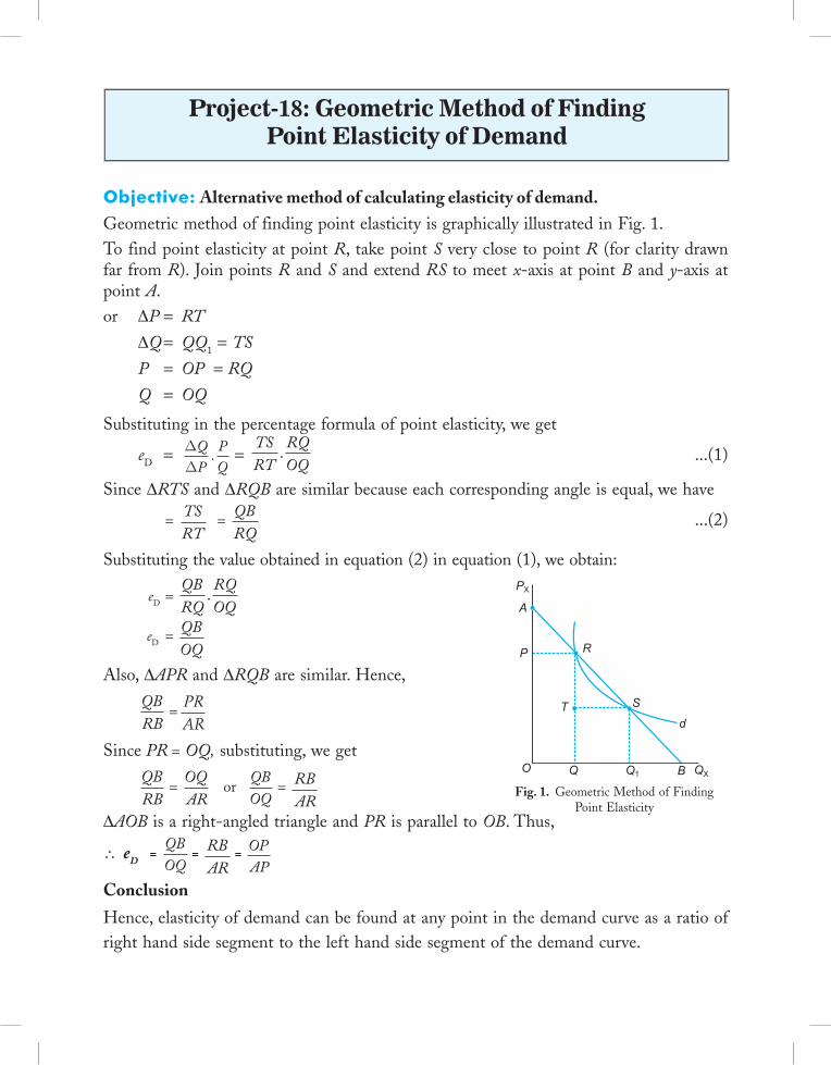
Objective: Alternative method of calculating elasticity of demand.Geometric method of finding point elasticity is graphically illustrated in Fig. 1.To find point elasticity at point R, take point S very close to point R (for clarity drawn far from R). Join points R and S and extend RS to meet x-axis at point B and y-axis at point A.or DP = RT
DQ = QQ1 = TS
P = OP = RQ
Q = OQ
Substituting in the percentage formula of point elasticity, we get
eD = DD
QP
PQ
. = TSRT
RQOQ
. ...(1)
Since DRTS and DRQB are similar because each corresponding angle is equal, we have
= TSRT
= QBRQ
...(2)
Substituting the value obtained in equation (2) in equation (1), we obtain:
eD = QBRQ
RQOQ
.
eD = QBOQ
Also, DAPR and DRQB are similar. Hence,
QBRB
=
Since PR = OQ, substituting, we get
QBRB
= OQAR
or QBOQ
= RBAR
DAOB is a right-angled triangle and PR is parallel to OB. Thus,
\ eD = QBOQ
= RBAR
= OPAP
Conclusion
Hence, elasticity of demand can be found at any point in the demand curve as a ratio of right hand side segment to the left hand side segment of the demand curve.
PX
A
PR
T S
d
O Q Q1 QXB
Fig. 1. Geometric Method of Finding Point Elasticity
Project-18: Geometric Method of Finding Point Elasticity of Demand
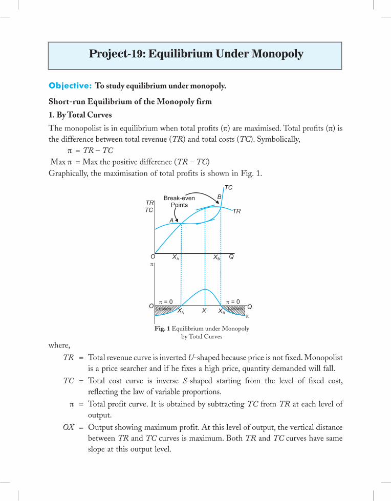
Objective: To study equilibrium under monopoly.
Short-run Equilibrium of the Monopoly firm
1. By Total Curves
The monopolist is in equilibrium when total profits (π) are maximised. Total profits (π) is the difference between total revenue (TR) and total costs (TC). Symbolically, π = TR – TC Max π = Max the positive difference (TR – TC)Graphically, the maximisation of total profits is shown in Fig. 1.
A B
A B
Fig. 1 Equilibrium under Monopolyby Total Curves
where,
TR = Total revenue curve is inverted U-shaped because price is not fixed. Monopolist is a price searcher and if he fixes a high price, quantity demanded will fall.
TC = Total cost curve is inverse S-shaped starting from the level of fixed cost, reflecting the law of variable proportions.
π = Total profit curve. It is obtained by subtracting TC from TR at each level of output.
OX = Output showing maximum profit. At this level of output, the vertical distance between TR and TC curves is maximum. Both TR and TC curves have same slope at this output level.
Project-19: Equilibrium Under Monopoly
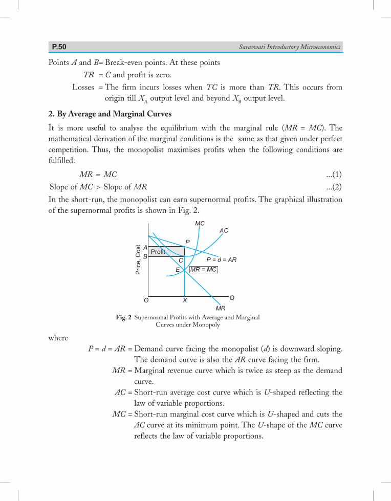
Saraswati Introductory MicroeconomicsP.50
Points A and B = Break-even points. At these points
TR = C and profit is zero.
Losses = The firm incurs losses when TC is more than TR. This occurs from origin till XA output level and beyond XB output level.
2. By Average and Marginal Curves
It is more useful to analyse the equilibrium with the marginal rule (MR = MC). The mathematical derivation of the marginal conditions is the same as that given under perfect competition. Thus, the monopolist maximises profits when the following conditions are fulfilled:
MR = MC ...(1)
Slope of MC > Slope of MR ...(2)
In the short-run, the monopolist can earn supernormal profits. The graphical illustration of the supernormal profits is shown in Fig. 2.
Fig. 2 Supernormal Profits with Average and Marginal Curves under Monopoly
where P = d = AR = Demand curve facing the monopolist (d) is downward sloping.
The demand curve is also the AR curve facing the firm. MR = Marginal revenue curve which is twice as steep as the demand
curve. AC = Short-run average cost curve which is U-shaped reflecting the
law of variable proportions. MC = Short-run marginal cost curve which is U-shaped and cuts the
AC curve at its minimum point. The U-shape of the MC curve reflects the law of variable proportions.
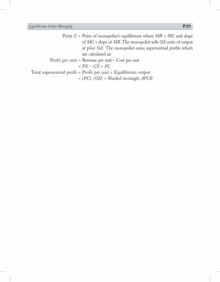
Equilibrium Under Monopoly P.51
Point E = Point of monopolist’s equilibrium where MR = MC and slope of MC > slope of MR. The monopolist sells OX units of output at price OA. The monopolist earns supernormal profits which are calculated as:
Profit per unit =Revenue per unit – Cost per unit = PX – CX = PC Total supernormal profit = Profit per unit × Equilibrium output = (PC). (OX) = Shaded rectangle APCB
Objective: To compare price and output under perfect competition and monopoly.
Perfectly competitive firm will produce when: P = MC and slope of MC > OMonopoly firm will produce when: MR = MCand slope of MC > Slope of MRThe perfectly competitive firm is in equilibrium at point E (Fig. 1).
Fig. 1 Comparison of Price and Output under Perfect Competition and Monopoly
where PP = Price under perfect competition OP =Output under perfect competition PM = Price under monopoly OM =Output under monopoly
At this point
Point E = P = MC. The firm produces its profit maximising level of output OP at price PP.
The monopolist is in equilibrium at point E1 where MR = MC producing his profit maximising level of output OM at price PM.
ConclusionComparing, equilibrium price under perfect competiton is lower than that under monopoly (PP < PM) and equilibrium output under perfect competition is higher than that under monopoly (OP > OM).
Project-20: Comparison of Price and Output Under Monopoly and Perfect Competition

NOTES
. . . . . . . . . . . . . . . . . . . . . . . . . . . . . . . . . . . . . . . . . . . . . . . . . . . . . . . . . . . . . . . . . . . . . . . . . . . . . . . . . . . . .
. . . . . . . . . . . . . . . . . . . . . . . . . . . . . . . . . . . . . . . . . . . . . . . . . . . . . . . . . . . . . . . . . . . . . . . . . . . . . . . . . . . . .
. . . . . . . . . . . . . . . . . . . . . . . . . . . . . . . . . . . . . . . . . . . . . . . . . . . . . . . . . . . . . . . . . . . . . . . . . . . . . . . . . . . . .
. . . . . . . . . . . . . . . . . . . . . . . . . . . . . . . . . . . . . . . . . . . . . . . . . . . . . . . . . . . . . . . . . . . . . . . . . . . . . . . . . . . . .
. . . . . . . . . . . . . . . . . . . . . . . . . . . . . . . . . . . . . . . . . . . . . . . . . . . . . . . . . . . . . . . . . . . . . . . . . . . . . . . . . . . . .
. . . . . . . . . . . . . . . . . . . . . . . . . . . . . . . . . . . . . . . . . . . . . . . . . . . . . . . . . . . . . . . . . . . . . . . . . . . . . . . . . . . . .
. . . . . . . . . . . . . . . . . . . . . . . . . . . . . . . . . . . . . . . . . . . . . . . . . . . . . . . . . . . . . . . . . . . . . . . . . . . . . . . . . . . . .
. . . . . . . . . . . . . . . . . . . . . . . . . . . . . . . . . . . . . . . . . . . . . . . . . . . . . . . . . . . . . . . . . . . . . . . . . . . . . . . . . . . . .
. . . . . . . . . . . . . . . . . . . . . . . . . . . . . . . . . . . . . . . . . . . . . . . . . . . . . . . . . . . . . . . . . . . . . . . . . . . . . . . . . . . . .
. . . . . . . . . . . . . . . . . . . . . . . . . . . . . . . . . . . . . . . . . . . . . . . . . . . . . . . . . . . . . . . . . . . . . . . . . . . . . . . . . . . . .
. . . . . . . . . . . . . . . . . . . . . . . . . . . . . . . . . . . . . . . . . . . . . . . . . . . . . . . . . . . . . . . . . . . . . . . . . . . . . . . . . . . . .
. . . . . . . . . . . . . . . . . . . . . . . . . . . . . . . . . . . . . . . . . . . . . . . . . . . . . . . . . . . . . . . . . . . . . . . . . . . . . . . . . . . . .
. . . . . . . . . . . . . . . . . . . . . . . . . . . . . . . . . . . . . . . . . . . . . . . . . . . . . . . . . . . . . . . . . . . . . . . . . . . . . . . . . . . . .
. . . . . . . . . . . . . . . . . . . . . . . . . . . . . . . . . . . . . . . . . . . . . . . . . . . . . . . . . . . . . . . . . . . . . . . . . . . . . . . . . . . . .
. . . . . . . . . . . . . . . . . . . . . . . . . . . . . . . . . . . . . . . . . . . . . . . . . . . . . . . . . . . . . . . . . . . . . . . . . . . . . . . . . . . . .
. . . . . . . . . . . . . . . . . . . . . . . . . . . . . . . . . . . . . . . . . . . . . . . . . . . . . . . . . . . . . . . . . . . . . . . . . . . . . . . . . . . . .
. . . . . . . . . . . . . . . . . . . . . . . . . . . . . . . . . . . . . . . . . . . . . . . . . . . . . . . . . . . . . . . . . . . . . . . . . . . . . . . . . . . . .
. . . . . . . . . . . . . . . . . . . . . . . . . . . . . . . . . . . . . . . . . . . . . . . . . . . . . . . . . . . . . . . . . . . . . . . . . . . . . . . . . . . . .
. . . . . . . . . . . . . . . . . . . . . . . . . . . . . . . . . . . . . . . . . . . . . . . . . . . . . . . . . . . . . . . . . . . . . . . . . . . . . . . . . . . . .
. . . . . . . . . . . . . . . . . . . . . . . . . . . . . . . . . . . . . . . . . . . . . . . . . . . . . . . . . . . . . . . . . . . . . . . . . . . . . . . . . . . . .
. . . . . . . . . . . . . . . . . . . . . . . . . . . . . . . . . . . . . . . . . . . . . . . . . . . . . . . . . . . . . . . . . . . . . . . . . . . . . . . . . . . . .
. . . . . . . . . . . . . . . . . . . . . . . . . . . . . . . . . . . . . . . . . . . . . . . . . . . . . . . . . . . . . . . . . . . . . . . . . . . . . . . . . . . . .