Sarah Maria Brockhaus -...
190
Sarah Maria Brockhaus Boosting Functional Regression Models Dissertation an der Fakult¨ at f¨ ur Mathematik, Informatik und Statistik der Ludwig-Maximilians-Universit¨ at M¨ unchen Eingereicht am 22. Juni 2016
Transcript of Sarah Maria Brockhaus -...
Sarah Maria Brockhaus
Boosting Functional Regression Models
Dissertation an der Fakultat fur Mathematik, Informatik und Statistik
der Ludwig-Maximilians-Universitat Munchen
Eingereicht am 22. Juni 2016

ii

Sarah Maria Brockhaus
Boosting Functional Regression Models
Dissertation an der Fakultat fur Mathematik, Informatik und Statistik
der Ludwig-Maximilians-Universitat Munchen
Eingereicht am 22. Juni 2016

Erste Berichterstatterin: Prof. Dr. Sonja Greven
Zweiter Berichterstatter: Prof. Dr. Matthias Schmid
Tag der Disputation: 31. August 2016

Acknowledgments
My gratitude goes to everyone who helped with this thesis. I wish to thank . . .
. . . my supervisor Sonja Greven for her support and encouragement, for insightful discussions, for the
freedom to subsequently choose new projects, for the help with academic English, for commenting
on all my drafts and for knowing that my self-imposed deadlines were always too optimistic.
. . . all the other coauthors who worked with me on the papers that form the basis of the thesis.
Thanks to Torsten Hothorn and Fabian Scheipl for the help with boosting, notation, paper
writing and proofreading; and for the encouragement to implement a new R package. Thanks to
Michael Melcher and Friedrich Leisch for the explanations about fermentations, the discussions
on model building and variable selection, proofreading and the great time in Vienna. Thanks
to Andreas Fuest and Andreas Mayr for sharing their knowledge on time series analysis and on
boosting GAMLSS and for the comments on the paper draft.
. . . Matthias Schmid who agreed to take the job as external examiner of the thesis.
. . . the German Research Foundation (DFG) for funding the major part of my work as part of the
Emmy Noether Junior Research Group “Statistical Methods for Longitudinal Functional Data”
(Emmy Noether grant GR 3793/1-1).
. . . Benjamin Hofner for explaining some of the internal workings of mboost as well as for general
support with the mboost package and with stability selection.
. . . David Rugamer for joining me in working on FDboost, for discussing new operators, methods
and functions and for his constantly good mood.
. . . all other users of FDboost who gave me feedback on the package; in particular, Almond Stocker
who found some well concealed bugs.
. . . all my colleagues in the working group and at the department for the great atmosphere and the
sociable breaks.
. . . my longstanding officemates Jona Cederbaum and Fabian Scheipl for sharing the office in the ups
and downs; for working, chatting, listening, swearing and laughing together; and for proofreading
parts of the thesis.
. . . Thomas, Hannah and Martin for proofreading parts of the thesis.
. . . my parents and Matthias–for everything.

vi

Zusammenfassung
In funktionaler Datenanalyse bestehen die Daten aus Funktionen, die auf stetigen Tragern definiert
sind. In der Praxis werden funktionale Variablen auf diskreten Gittern beobachtet. Regressionsmod-
elle sind ein wichtiges Werkzeug, um den Einfluss von Kovariablen auf eine Zielvariable zu modellieren;
fur funktionale Daten stellen sich besondere Herausforderungen. In dieser Arbeit wird eine generische
Modellklasse vorgeschlagen, die Skalar-auf-Funktion, Funktion-auf-Skalar und Funktion-auf-Funktion
Regression enthalt. Quantilsregression, generalisierte additive Modelle und generalisierte additive
Modelle fur Lage, Skala und Form sind in dieser Modellklasse enthalten indem eine passende Verlust-
funktion minimiert wird. Die additiven Pradiktoren konnen eine Vielzahl von Kovariableneffekten
enthalten, zum Beispiel lineare und glatte Effekte, sowie Interaktionseffekte von skalaren und funk-
tionalen Kovariablen.
Im ersten Teil der Arbeit werden funktionale lineare Array Modelle eingefuhrt. Diese konnen
angewendet werden, wenn die Zielgroße auf einem gemeinsamen Gitter beobachtet wird und die
Kovariablen nicht uber den Trager der Zielgroße variieren. Bei Array Modellen wird die Kronecker-
Struktur in der Designmatrix ausgenutzt, um computationale Effizienz zu erzielen. Im zweiten Teil
liegt der Fokus auf Modellen ohne Array-Struktur um Situation abzubilden, in denen die Zielgroße
auf irregularen Gittern beobachtet wird und/oder die Kovariablen uber den Trager der Zielgroße
variieren. Das beinhaltet insbesondere Modelle mit funktionalen historischen Effekten. Wenn funk-
tionale Ziel- und Einflussgroße jeweils uber das gleiche Zeitintervall beobachtet werden, modelliert ein
funktionaler historischer Effekt eine Beziehung zwischen Ziel- und Einflussgroße, sodass nur vergan-
gene Werte der Einflussgroße die Zielgroße beeinflussen konnen. In dieser Modellklasse sind Effekte
mit generelleren Integrationsgrenzen moglich, beispielsweise Effekte mit einem fixen Zeitfenster oder
zeitlicher Verzogerung. Im dritten Teil wird die Modellklasse auf generalisierte additive Modelle
fur Lage, Skala und Form erweitert. Bei diesen konnen alle Verteilungsparameter der konditionalen
Verteilung der Zielgroße von Kovariableneffekten abhangen. Indem jeder Verteilungsparameter uber
eine Link-Funktion mit einem linearen Pradiktor in Beziehung gesetzt wird, kann die konditionale
Verteilung der Zielgroße sehr flexibel modelliert werden.
Fur alle Teile der Dissertation wird die Schatzung mit komponentenweisen Gradienten-Boosting
durchgefuhrt. Boosting ist eine Ensemble-Methode, die eine Strategie von Aufteilen und Beherrschen
verfolgt, um ein erwartetes Verlustkriterium zu optimieren. Das stellt eine große Flexibilitat fur die
Regressionsmodelle zur Verfugung, da zum Beispiel Minimieren der Check-Funktion Quantilsregres-
sion und Minimieren der negativen log-likelihood generalisierte additive Modelle und generalisierte
additive Modelle fur Lage, Skala und Form liefert. Der Schatzer wird entlang des steilsten Gradienten-
abstiegs aktualisiert. Das Modell wird durch einfache (penalisierte) Regressionsmodelle dargestellt,
die sogenannten Basis-Lerner, die einzeln an den negativen Gradienten angepasst werden. In je-
dem Schritt wird nur der am besten vorhersagende Basis-Lerner ausgewahlt. Komponentenweises
Boosting erlaubt es, hochdimensionale Daten zu fitten und beinhaltet automatische, datengesteuerte
Variablenselektion. Um Boosting fur funktionale Daten anzupassen, wird der Verlust uber den Trager
der Zielgroße integriert und spezielle Basis-Lerner fur funktionale Effekte implementiert. Um die An-

viii
wendbarkeit von funktionalen Regressionsmodellen zu fordern, wird eine umfassende Implementation
der Methoden im R Paket FDboost zur Verfugung gestellt.
Die Flexibilitat der Modellklasse wird von mehreren Anwendungen aus verschiedenen Bereichen
beleuchtet. Einige Moglichkeiten von funktionalen linearen Array Modellen werden mit Daten zur
Aushartung von Harz in der Autoproduktion, Brennwerten von fossilen Brennstoffen und kanadischen
Klimadaten verdeutlicht. Diese erfordern Skalar-auf-Funktion, Funktion-auf-Skalar und Funktion-
auf-Funktion Regression. Die methodischen Entwicklungen fur nicht-Array Modelle sind durch eine
biotechnologische Anwendung zu Fermentationsprozessen motiviert. Dort soll eine wichtige Prozess-
variable mit einem historischen funktionalen Modell modelliert werden. Die motivierende Anwendung
fur die funktionalen generalisierten additiven Modelle fur Lage, Skala und Form ist eine Zeitreihe von
Aktienrenditen, bei der Erwartungswert und Standardabweichung abhangig von skalaren und funk-
tionalen Kovariablen modelliert werden.
Summary
In functional data analysis, the data consist of functions that are defined on a continuous domain. In
practice, functional variables are observed on some discrete grid. Regression models are important
tools to capture the impact of explanatory variables on the response and are challenging in the case
of functional data. In this thesis, a generic framework is proposed that includes scalar-on-function,
function-on-scalar and function-on-function regression models. Within this framework, quantile re-
gression models, generalized additive models and generalized additive models for location, scale and
shape can be derived by optimizing the corresponding loss functions. The additive predictors can
contain a variety of covariate effects, for example linear, smooth and interaction effects of scalar and
functional covariates.
In the first part, the functional linear array model is introduced. This model is suited for responses
observed on a common grid and covariates that do not vary over the domain of the response. Array
models achieve computational efficiency by taking advantage of the Kronecker product in the design
matrix. In the second part, the focus is on models without array structure, which are capable to
capture situations with responses observed on irregular grids and/or time-varying covariates. This
includes in particular models with historical functional effects. For situations, in which the functional
response and covariate are both observed over the same time domain, a historical functional effect
induces an association between response and covariate such that only past values of the covariate
influence the current value of the response. In this model class, effects with more general integration
limits, like lag and lead effects, can be specified. In the third part, the framework is extended to
generalized additive models for location, scale and shape where all parameters of the conditional
response distribution can depend on covariate effects. The conditional response distribution can be
modeled very flexibly by relating each distribution parameter with a link function to a linear predictor.
For all parts, estimation is conducted by a component-wise gradient boosting algorithm. Boost-
ing is an ensemble method that pursues a divide-and-conquer strategy for optimizing an expected
loss criterion. This provides great flexibility for the regression models. For example, minimizing
the check function yields quantile regression and minimizing the negative log-likelihood generalized
additive models for location, scale and shape. The estimator is updated iteratively to minimize the
loss criterion along the steepest gradient descent. The model is represented as a sum of simple (pe-
nalized) regression models, the so called base-learners, that separately fit the negative gradient in
each step where only the best-fitting base-learner is updated. Component-wise boosting allows for
high-dimensional data settings and for automatic, data-driven variable selection. To adapt boost-
ing for regression with functional data, the loss is integrated over the domain of the response and
base-learners suited to functional effects are implemented. To enhance the availability of functional
regression models for practitioners, a comprehensive implementation of the methods is provided in
the R add-on package FDboost.
The flexibility of the regression framework is highlighted by several applications from different
fields. Some features of the functional linear array model are illustrated using data on curing resin for
car production, heat values of fossil fuels and Canadian climate data. These require function-on-scalar,

x
scalar-on-function and function-on-function regression models, respectively. The methodological de-
velopments for non-array models are motivated by biotechnological data on fermentations, modeling
a key process variable by a historical functional model. The motivating application for functional
generalized additive models for location, scale and shape is a time series on stock returns where
expectation and standard deviation are modeled depending on scalar and functional covariates.
Contents
1 Introduction 1
1.1 Functional data analysis . . . . . . . . . . . . . . . . . . . . . . . . . . . . . . . . . . . 1
1.2 Functional regression models in a nutshell . . . . . . . . . . . . . . . . . . . . . . . . . 3
1.3 Short introduction to boosting . . . . . . . . . . . . . . . . . . . . . . . . . . . . . . . 5
1.4 Scope of this work . . . . . . . . . . . . . . . . . . . . . . . . . . . . . . . . . . . . . . 6
1.5 Contributing manuscripts . . . . . . . . . . . . . . . . . . . . . . . . . . . . . . . . . . 9
1.6 Software . . . . . . . . . . . . . . . . . . . . . . . . . . . . . . . . . . . . . . . . . . . . 10
2 Generic framework for functional regression 11
2.1 Generic model . . . . . . . . . . . . . . . . . . . . . . . . . . . . . . . . . . . . . . . . 11
2.2 Covariate effects . . . . . . . . . . . . . . . . . . . . . . . . . . . . . . . . . . . . . . . 12
2.3 Transformation and loss functions . . . . . . . . . . . . . . . . . . . . . . . . . . . . . 17
2.4 Estimation by gradient boosting . . . . . . . . . . . . . . . . . . . . . . . . . . . . . . 18
2.5 Comparison with existing frameworks . . . . . . . . . . . . . . . . . . . . . . . . . . . 20
3 The functional linear array model 23
3.1 Introduction . . . . . . . . . . . . . . . . . . . . . . . . . . . . . . . . . . . . . . . . . . 24
3.2 Model specification . . . . . . . . . . . . . . . . . . . . . . . . . . . . . . . . . . . . . . 26
3.3 Estimation . . . . . . . . . . . . . . . . . . . . . . . . . . . . . . . . . . . . . . . . . . 28
3.4 Estimation by gradient boosting . . . . . . . . . . . . . . . . . . . . . . . . . . . . . . 29
3.5 Simulation study . . . . . . . . . . . . . . . . . . . . . . . . . . . . . . . . . . . . . . . 32
3.6 Applications . . . . . . . . . . . . . . . . . . . . . . . . . . . . . . . . . . . . . . . . . . 35
3.6.1 Function-on-scalar regression: viscosity over time . . . . . . . . . . . . . . . . . 36
3.6.2 Scalar-on-function regression: spectral data of fossil fuels . . . . . . . . . . . . 38
3.6.3 Function-on-function regression: Canadian weather data . . . . . . . . . . . . . 41
3.7 Discussion . . . . . . . . . . . . . . . . . . . . . . . . . . . . . . . . . . . . . . . . . . . 43
4 Functional regression models with many historical effects 47
4.1 Introduction . . . . . . . . . . . . . . . . . . . . . . . . . . . . . . . . . . . . . . . . . . 48
4.2 The functional regression model with many historical effects . . . . . . . . . . . . . . . 49
4.2.1 Alternative parameterizations of the functional historical effect . . . . . . . . . 51
xii CONTENTS
4.2.2 Identifiability of the functional historical effect . . . . . . . . . . . . . . . . . . 52
4.3 Extension to the general model . . . . . . . . . . . . . . . . . . . . . . . . . . . . . . . 53
4.4 Estimation by gradient boosting . . . . . . . . . . . . . . . . . . . . . . . . . . . . . . 55
4.5 Simulation study . . . . . . . . . . . . . . . . . . . . . . . . . . . . . . . . . . . . . . . 57
4.6 Application in bioprocess monitoring . . . . . . . . . . . . . . . . . . . . . . . . . . . . 61
4.7 Discussion . . . . . . . . . . . . . . . . . . . . . . . . . . . . . . . . . . . . . . . . . . . 67
5 Signal regression models for location, scale and shape 69
5.1 Introduction . . . . . . . . . . . . . . . . . . . . . . . . . . . . . . . . . . . . . . . . . . 70
5.2 Generic model . . . . . . . . . . . . . . . . . . . . . . . . . . . . . . . . . . . . . . . . 72
5.3 Specification of effects . . . . . . . . . . . . . . . . . . . . . . . . . . . . . . . . . . . . 74
5.3.1 Signal regression terms . . . . . . . . . . . . . . . . . . . . . . . . . . . . . . . . 74
5.3.2 Choice of basis functions and identifiability . . . . . . . . . . . . . . . . . . . . 75
5.4 Estimation by gradient boosting . . . . . . . . . . . . . . . . . . . . . . . . . . . . . . 76
5.5 Estimation based on penalized maximum likelihood . . . . . . . . . . . . . . . . . . . . 79
5.5.1 The gamlss algorithm using backfitting . . . . . . . . . . . . . . . . . . . . . . 80
5.5.2 Laplace Approximate Marginal Likelihood with nested optimization . . . . . . 80
5.6 Comparison of estimation methods . . . . . . . . . . . . . . . . . . . . . . . . . . . . . 81
5.7 Model choice and diagnostics . . . . . . . . . . . . . . . . . . . . . . . . . . . . . . . . 81
5.8 Application to financial returns of the Commerzbank stock . . . . . . . . . . . . . . . 83
5.8.1 Model choice . . . . . . . . . . . . . . . . . . . . . . . . . . . . . . . . . . . . . 84
5.8.2 Results . . . . . . . . . . . . . . . . . . . . . . . . . . . . . . . . . . . . . . . . 88
5.9 Simulation studies . . . . . . . . . . . . . . . . . . . . . . . . . . . . . . . . . . . . . . 89
5.9.1 Simulation study for the application on stock returns . . . . . . . . . . . . . . . 90
5.9.2 General simulation study . . . . . . . . . . . . . . . . . . . . . . . . . . . . . . 91
5.10 Discussion . . . . . . . . . . . . . . . . . . . . . . . . . . . . . . . . . . . . . . . . . . . 91
6 On the practical use of the R package FDboost 93
6.1 Introduction . . . . . . . . . . . . . . . . . . . . . . . . . . . . . . . . . . . . . . . . . . 93
6.2 The generic functional regression model . . . . . . . . . . . . . . . . . . . . . . . . . . 94
6.3 Gradient boosting . . . . . . . . . . . . . . . . . . . . . . . . . . . . . . . . . . . . . . 96
6.4 Case study: Canadian weather data . . . . . . . . . . . . . . . . . . . . . . . . . . . . 97
6.5 The package FDboost . . . . . . . . . . . . . . . . . . . . . . . . . . . . . . . . . . . . 98
6.5.1 Specification of functional and scalar response . . . . . . . . . . . . . . . . . . . 99
6.5.2 Potential covariate effects: base-learners . . . . . . . . . . . . . . . . . . . . . . 100
6.5.3 Transformation and loss functions: families . . . . . . . . . . . . . . . . . . . . 106
6.5.4 Model tuning and early stopping . . . . . . . . . . . . . . . . . . . . . . . . . . 109
6.5.5 Methods to extract and display results . . . . . . . . . . . . . . . . . . . . . . . 111
6.6 Discussion . . . . . . . . . . . . . . . . . . . . . . . . . . . . . . . . . . . . . . . . . . . 114

CONTENTS xiii
7 Discussion 115
7.1 Concluding summary . . . . . . . . . . . . . . . . . . . . . . . . . . . . . . . . . . . . . 115
7.2 Outlook . . . . . . . . . . . . . . . . . . . . . . . . . . . . . . . . . . . . . . . . . . . . 117
Appendices 121
A Identifiability 123
A.1 Functional response: identifiability constraints for FLAMs . . . . . . . . . . . . . . . . 123
A.2 Functional covariates: identifiability of historical effects . . . . . . . . . . . . . . . . . 125
A.2.1 Marginal design matrices . . . . . . . . . . . . . . . . . . . . . . . . . . . . . . 125
A.2.2 Checking for rank deficiency of the design matrix . . . . . . . . . . . . . . . . . 126
A.2.3 Effect of the penalty in the case of a rank deficient design matrix . . . . . . . . 127
A.2.4 Responses with curve-specific grids . . . . . . . . . . . . . . . . . . . . . . . . . 128
B Details on the simulation study for FLAM models 129
B.1 Examples for data generation and model fit . . . . . . . . . . . . . . . . . . . . . . . . 129
B.2 Computation times . . . . . . . . . . . . . . . . . . . . . . . . . . . . . . . . . . . . . . 129
C Details for simulation and application of the models with historical effects 133
C.1 Data generation in the simulation study . . . . . . . . . . . . . . . . . . . . . . . . . . 133
C.2 Further results of the simulation study . . . . . . . . . . . . . . . . . . . . . . . . . . . 134
C.3 Data preprocessing and further results for the application to fermentation processes . 138
D Implementation of signal GAMLSS and further details on application and simu-
lation 143
D.1 Details on the implementation of the estimation methods . . . . . . . . . . . . . . . . 143
D.1.1 Used R packages . . . . . . . . . . . . . . . . . . . . . . . . . . . . . . . . . . . 143
D.1.2 Example R code . . . . . . . . . . . . . . . . . . . . . . . . . . . . . . . . . . . 144
D.2 Further results of the application on stock returns . . . . . . . . . . . . . . . . . . . . 147
D.3 Details of the general simulation study . . . . . . . . . . . . . . . . . . . . . . . . . . . 148
E Further details on the R package FDboost 157
E.1 Base-learners for functional covariates . . . . . . . . . . . . . . . . . . . . . . . . . . . 157
E.2 Implementation of the row tensor product and the Kronecker product bases . . . . . . 158
References 161

xiv CONTENTS

Chapter 1
Introduction
1.1 Functional data analysis
Functional data analysis (FDA, see, e.g., Ramsay and Silverman, 2005) deals with the analysis and
theory of variables that have a functional nature. This means that the observation units are functions
instead of scalars or vectors. The analysis of functional data is becoming increasingly important as
technological advances generate more and more such data in fields like medicine, biology, linguistics,
ecology and finance (see Ullah and Finch, 2013, for an overview on applications). Depending on the
dimension, functional data consist of curves, surfaces or images. The domain of the functions can be,
for instance, time, space, wavelength or a combination of those for functions in higher dimensions.
Examples for functional data are growth curves, blood markers recorded over time, spectroscopic
measurements recorded over a span of wavelengths, reach trajectories and brain scans. Functional
variables are theoretically infinite-dimensional as they live in function space. In practice, however, the
functions are only recorded at a finite number of discrete grid points, which yields vector observations.
One reason that a variable may be considered a functional variable is that, at least theoretically, it
could be measured on arbitrary fine grids. This leads to the decision to treat each vector of observation
points as a structured object, i.e., as functional variable, and not just as single observation points.
Consequently the functional variable can be represented by a functional model (e.g., Cuevas, 2014).
Typically, the true underlying functions are assumed to be smooth. This allows the analysis of function
characteristics, e.g., slope and curvature. The analysis of functional data requires the combination of
information within and between functions in a smart way.
The fundamental ideas of FDA were laid out in Ramsay and Silverman (2005, first edition
published in 1997) including smoothing and registration of functional data, functional principal
components (FPCs), functional analysis of derivatives as well as functional linear regression models.
Ramsay and Silverman (2005) focus on independent and identically distributed (iid) samples of
curves that are measured on dense, common grids. In recent years, several books on different
aspects of FDA appeared. Ferraty and Vieu (2006) elaborate nonparametric methods for functional
data focusing on prediction and classification. They highlight methods for dependent functional

2 1. Introduction
data and treat asymptotics. Horvath and Kokoszka (2012) cover inference for dependent and
independent functional data. A more theoretical overview is given in Hsing and Eubank (2015),
who also comment on methods for functional data that are not observed on dense, common grids.
For recent review articles on FDA, see Cuevas (2014); Wang et al. (2016); Goia and Vieu (2016)
and for a focus on dependent functional data, Kokoszka (2012). Ullah and Finch (2013) give a
systematic review of applications of FDA. The collections by Ferraty (2011) and Ferraty and Romain
(2011) contain chapters from various researchers in the field giving an idea of the many facets of FDA.
Most work in the area focuses on situations in which the functional variables are real-valued
curves. In this case, the sample of a functional variable Y (t), with t ∈ T and T a closed interval
on R, consists of i = 1, . . . , N curves yi(tig) observed at grid points (ti1, . . . , tiGi)>. The functional
variable could be, for example, growth curves of N individuals measured over a certain time
interval T at several time-points. A common assumption is that the observed curves are realizations
of a stochastic process in a Hilbert space, for example, the space of square integrable real functions
on the interval T , L2(T ), with inner product 〈x, y〉 =∫T x(t)y(t) dt.
The sampling scheme, i.e., the number and regularity of grid points at which the functions are
observed, is an important property of a functional data sample, as it influences the possible analysis
methods and their properties. A rough differentiation between dense and sparse functional data can
be made, where ’dense’ refers to data observed on a dense grid whereas ’sparse’ refers to data observed
on sparse and often irregular grids. One potential definition of ’dense grid’ can be based on the con-
vergence rate of the estimated mean function; for a thorough discussion, see Zhang and Wang (2016).
Typical examples for densely observed functional data are automatically recorded measurements, like
spectroscopic data. Sparse and irregular grids are often encountered in longitudinal data, such as
measurements of blood markers in patients over a period of time with irregular follow-ups. Irregular
grids can also occur when the functional variable is observed with missing values.
The functions are usually observed with measurement error. Assuming additive errors, we observe
proxies yi(tig) = yi(tig) + εitig that are the sum of the true functional variable yi(tig) and errors εitig .
The errors εitig are often assumed to be white noise that is independent within and across functions.
Depending on the data situation, various tools for estimating the true underlying functions from the
observed values have been developed. The denoising normally implies some kind of smoothing. A
common approach is to use a basis representation of the functional data. This has the additional
advantage of dimension reduction, as it projects the data into the space spanned by the basis func-
tions. A popular choice for the basis are the first few FPCs of the functional variable (e.g., Ramsay
and Silverman, 2005; Yao et al., 2005a), (penalized) splines, wavelets or Fourier bases. Alternative
smoothing procedures are local smoothing methods, for example, by using kernel functions (Ferraty
and Vieu, 2006; Zhang and Chen, 2007). Another issue is the registration or alignment of curves to
compensate for phase variation, i.e., variation in t direction (horizontal), as most methods are tailored
to detect variation in the amplitudes (vertical), i.e., variation in y direction (cf., Ramsay and Li, 1998;
Marron et al., 2014).

1.2 Functional regression models in a nutshell 3
Regarding mean and variance of a one-dimensional functional variable Y (t) in L2(T ), the mean
function µ(t) = E(Y (t)) is a curve and the covariance function is a surface. The estimation of
mean and variance becomes more difficult for sparse functional data, for data observed with (large)
measurement error and for dependent functional data. Again, many estimation methods exist; see,
e.g., Wang et al. (2016) for an overview. In order to define the median or quantiles of a functional
variable, it is necessary to define an order statistic for functional data. One possibility is to use
so-called depth functions, which measure how deep an observed function lies within a sample of
functions. This provides a center-outward ordering of the observed functions (e.g., Lopez-Pintado
and Romo, 2009). The depth-median is defined to be the deepest function.
In the FDA literature, functional counterparts for many statistical tools from multivariate statis-
tics can be found. These include functional principal component analysis (FPCA), regression, classi-
fication, and clustering methods; see Shang (2014) for a review on FPCA, Morris (2015) on functional
regression and Jacques and Preda (2014) on functional clustering. As this thesis focuses on regres-
sion models for functional data, a short introduction to functional regression models is given in the
subsequent section (Section 1.2).
1.2 Functional regression models in a nutshell
In recent years, a variety of regression methods for functional data have been developed and dis-
cussed. In principle, one can distinguish between methods for functional response and/or functional
covariates resulting in scalar-on-function, function-on-scalar and function-on-function regression. For
a recent review article on regression methods with functional data, see Morris (2015).
Scalar-on-function regression. The scalar-on-function model was introduced by Ramsay and
Dalzell (1991) as the linear functional model
yi = β0 +
∫Sxi(s)β(s) ds+ εi, (1.1)
with continuous response yi, i = 1, . . . , N , functional covariate xi(s), s ∈ S, intercept β0, functional
coefficient β(s) and errors εiiid∼ N(0, σ2). Divers generalizations and extensions of model (1.1)
allow, for example, for different response distributions, non-linearity of the functional effect and
further covariate effects. For response distributions from the exponential family, generalized linear
models (GLMs, Nelder and Wedderburn, 1972) with linear effects of functional covariates (e.g., Marx
and Eilers, 1999; Ramsay and Silverman, 2005; Muller and Stadtmuller, 2005; Goldsmith et al.,
2011; Gertheiss et al., 2013) have been proposed. To abandon linearity, functional counterparts
of generalized additive models (GAMs, Hastie and Tibshirani, 1986) have been introduced, which
model non-linear effects of functional covariates (e.g., James and Silverman, 2005; McLean et al.,
2014). A distribution-free approach for continuous responses is quantile regression (Koenker, 2005).
Quantile regression with functional covariates has been discussed by Ferraty et al. (2005); Cardot
4 1. Introduction
et al. (2005) and Chen and Muller (2012a). An important difference between the models is the choice
of the basis representation for the functional covariate and/or for the functional coefficient. The
basis representation can be combined with additional regularization by a penalty. Typical choices for
the basis functions are FPCs, (penalized) splines or wavelets. Other issues are denoising the observed
functional covariates and dealing with irregularly or sparsely observed functional covariates. These
issues can be addressed, for example, by FPCA. Moreover, the models can be estimated by multiple
fitting algorithms. Mostly, (penalized) maximum likelihood approaches are used. A systematic
comparison between FPC based and functional partial least squares regression for scalar-on-function
regression can be found in Febrero-Bande et al. (2015). Ferraty et al. (2005, 2007) adopt a different
approach based on nonparametric, kernel methods to estimate scalar-on-function regression models.
These models can be used for prediction but do not provide interpretable coefficient terms.
Function-on-scalar regression. A linear regression model with functional response yi(t), i = 1, . . . , N ,
t ∈ T , and scalar covariates xij , j = 1, . . . , J , is
yi(t) = β0(t) +
J∑j=1
xijβj(t) + εi(t), (1.2)
where βj(t) is the functional coefficient that gives the effect of the jth covariate on the response
at point t and εi(t) are error curves. The errors are often assumed to be iid, mean zero Gaussian
processes with a specified auto-covariance to model the within-function covariance along t. It is
common to split the error curves into a smooth curve-specific random effect ei(t) and white noise
residual errors εit ∼ N(0, σ2) such that εi(t) = ei(t) + εit. If all covariates are factor variables, model
(1.2) can be seen as a model for functional analysis of variance (FANOVA, see Zhang, 2013, for an
overview). Multiple approaches have been proposed to model the conditional mean of a functional
response in the setting of independent (e.g., Reiss et al., 2010) and dependent data (e.g., Morris
and Carroll, 2006; Baladandayuthapani et al., 2008; Di et al., 2009; Greven et al., 2010; Chen and
Muller, 2012b; Cederbaum et al., 2016). Again, the methods differ in basis expansion, regularization
and fitting methods. For functional response regression, modeling of within-curve correlation is an
important issue. Most methods include rather strict assumptions on the within-curve correlation
structure and are only suitable for functional responses observed on a fine common grid.
Function-on-function regression. For functional response yi(t) and functional covariate xi(s),
Ramsay and Dalzell (1991) introduced the linear functional model
yi(t) = β0(t) +
∫Sxi(s)β(s, t) ds+ εi(t), (1.3)
where β(s, t) is a functional coefficient surface and εi(t) are error curves. This model combines the
concepts of functional response and functional covariate regression models. Extensions concerning
the response distribution, non-linearity of the effect and the inclusion of further covariate effects have
1.3 Short introduction to boosting 5
been discussed. Various basis expansions, regularization techniques and estimation methods have
been proposed, see, e.g., Yao et al. (2005b) and Wu and Muller (2011) for FPC based methods for
sparsely observed responses and Antoch et al. (2010) for a spline based method. For a non-linear effect
of the functional covariate, see Muller and Yao (2008). Ferraty et al. (2012) consider a nonparametric
kernel approach.
Concerning the support of the coefficient surface β(s, t) in model (1.3), constrained versions with
integration limits depending on the current point t exist, yielding
yi(t) = β0(t) +
∫ u(t)
l(t)xi(s)β(s, t) ds+ εi(t). (1.4)
If the functional response and the functional covariate are both observed on the same domain
T = [T1, T2], the limiting case [l(t), u(t)] = [t, t] corresponds to the concurrent effect xi(t)β(t)
(Ramsay and Silverman, 2005, Chap. 14), which is a special case of a varying-coefficient model
(Hastie and Tibshirani, 1993). For integration limits [l(t), u(t)] = [T1, t], the coefficient surface is
defined on the lower triangle and only past and concurrent values of xi(s) can influence yi(t), yielding
the historical functional linear model (Malfait and Ramsay, 2003; Harezlak et al., 2007). Historical
functional effects are especially suited when the functional response and the functional covariate
are both observed over the same time interval, as then the response is only influenced by covariate
observations up to the current time-point of the response.
Flexible frameworks for functional regression models. Regression models for functional response
and many covariate effects including functional terms, have been proposed in a mixed models
framework (Ivanescu et al., 2015; Scheipl et al., 2015, 2016) and in a Bayesian context (Morris
and Carroll, 2006; Meyer et al., 2015). These general frameworks include function-on-scalar and
function-on-function regression models. They greatly expand the flexibility of models (1.2), (1.3)
and (1.4) by allowing for response distributions from the exponential family and for many covariate
effects including linear and non-linear effects of scalar and functional variables as well as interaction
effects. A comparison between these frameworks and the framework based on boosting that is
proposed in this thesis is given in Section 2.5.
In this thesis, a general framework for functional regression models is proposed in which the
estimation is conducted by a component-wise gradient boosting algorithm. This complements
existing estimation methods for functional regression models.
1.3 Short introduction to boosting
Boosting was originally a black box machine learning algorithm for supervised learning and has
been developed to fit interpretable statistical models; see, e.g., Mayr et al. (2014a) for a review on the
history of boosting. A theoretical question led to the development of the first boosting algorithm. The
6 1. Introduction
question was whether it is possible to construct a strong learner that is an almost perfect classification
rule from a set of weak learners, which are only slightly better than random guessing. As an answer,
Freund and Schapire (1996, 1997) developed the first successful boosting algorithm, called ‘AdaBoost’
for adaptive boosting, which is suited for binary classification. The performance of weak learners,
which are later called ’base-learners’ in the boosting context, can be iteratively improved and combined
(i.e. boosted) to create a strong learner. Schapire and Freund (2012) explain the underlying idea of
boosting as “forming a very smart committee of grossly incompetent but carefully selected members.”
Variants of AdaBoost have been discussed in the machine learning community (e.g., Schapire, 2003)
and in statistics (e.g., Breiman, 1999; Friedman, 2001; Buhlmann and Hothorn, 2007; Mayr et al.,
2014b). Boosting has been shown to be competitive in comparison with other classification algorithms
in many applications (e.g., Breiman, 1998; Bauer and Kohavi, 1999).
Breiman (1998, 1999) showed that AdaBoost can be seen as a steepest gradient descent algorithm
in function space. Friedman et al. (2000) and Friedman (2001) linked boosting to statistical modeling,
interpreting it as a method for function estimation. This laid the basis for the use of boosting
outside of the classification context, e.g., for (generalized) regression (Ridgeway, 1999; Friedman,
2001; Buhlmann and Yu, 2003; Tutz and Binder, 2006), survival analysis (Hothorn et al., 2006;
Binder and Schumacher, 2008; Most and Hothorn, 2015) and density estimation (Ridgeway, 2002;
Hothorn et al., 2013). More recently, boosting algorithms to fit regression models beyond the mean
were developed. Examples include boosting quantile and expectile regression models (Fenske et al.,
2011; Sobotka and Kneib, 2012, respectively), boosting generalized additive models for location scale
and shape (GAMLSS, Mayr et al., 2012) and boosting conditional transformation models (Hothorn
et al., 2013).
The possible covariate effects are determined by the specified base-learners. Simple (penalized)
regression models as well as trees and tree stumps are commonly used. In the context of statistical
boosting for regression models, linear and smooth base-learners can be specified, resulting in linear
and additive models respectively.
We use a gradient boosting algorithm for statistical modeling (Friedman, 2001), where the base-
learners are simple (penalized) regression models and the optimum is searched along the steepest
gradient descent. We use a component-wise gradient boosting algorithm (see, e.g., Buhlmann and
Hothorn, 2007) that iteratively fits the negative gradient of the loss to each base-learner separately
and only updates the best-fitting base-learner in each step. Thus, models for high-dimensional data
settings with more covariates than observations can be estimated and variable selection is done in-
herently as base-learners that are never selected for the update are excluded from the model.
1.4 Scope of this work
This thesis proposes a general framework for functional regression models estimated by a component-
wise gradient boosting algorithm. The modeling framework has a modular setup allowing the combi-
nation of various choices for the model components:
1.4 Scope of this work 7
1. The characteristic of the conditional response distribution that is modeled: for example, the
mean (composed with a link function), the median, a quantile, an expectile and other distribu-
tion parameters can be modeled by minimizing an adequate loss function.
2. The specification of possible covariate effects in base-learners: for example, linear and smooth
effects of scalar covariates, linear effects of functional covariates, interaction effects and group-
specific effects. Various basis functions for the smooth effects are possible, e.g., P-splines (Eilers
and Marx, 1996) and FPC basis functions.
The estimation by gradient boosting enables most of this flexibility. The desired features of the
conditional response distribution are modeled by minimizing the corresponding loss function. Models
with more covariate effects than observations are feasible as the component-wise algorithm runs
through the base-learners one by one and only updates the best performing base-learner in each
step. This provides the variable selection property as base-learners never selected for the update
are excluded from the model. Regression models beyond the mean are of growing interest (see, e.g.,
Kneib, 2013). In this context, GAMLSS (Rigby and Stasinopoulos, 2005) allow modeling not only
the mean but, more generally, all distribution parameters of the conditional response distribution
depending on covariate effects. Referring to the fact that in GAMLSS all distribution parameters are
modeled, Klein et al. (2015) call such models ’distributional regression’. Other pathways for regression
beyond the mean are quantile (Koenker and Bassett, 1978; Koenker, 2005) and expectile (Newey and
Powell, 1987; Schnabel and Eilers, 2009) regression. We transfer models for scalar response to models
for functional response by computing the loss as a function over the domain of the response and
integrating this loss function over the domain of the response.
Neither the estimation of functional regression models in high-dimensional data situations (’small
p large N ’) nor variable selection are widely addressed in functional regression models (Morris, 2015).
Here, high-dimensional data and variable selection are meant on the level of many covariates, not
within a single functional variable. Thus, ’high-dimensional’ refers to situations where the number of
covariates exceeds the number of cases. In FDA, the term ’high-dimensional’ is sometimes also used
to refer to a functional variable, for which the number of grid points on which it is observed is higher
than the number of observed functions. With the term ’variable selection’, we refer to the selection
of relevant variables and not to the selection of relevant regions of a single functional covariate, as is
the case in James et al. (2009) and Tutz and Gertheiss (2010).
We discuss several variants of the generic model, which are each suited to certain data sit-
uations and modeling requirements. Within each chapter, one or more data applications are
analyzed giving examples of possible models. The theoretical framework is accompanied by
freely available software, in order to make the methods readily available for users. All methods are
implemented in the R (R Core Team, 2015) add-on package FDboost (Brockhaus and Rugamer, 2016).
Chapter 2 introduces the generic additive regression model and shows how the models dis-
cussed in Chapters 3 to 5 can be embedded in one common framework. Furthermore, the differences
between the models and the use-cases of each are briefly described. We shortly introduce the
8 1. Introduction
component-wise gradient boosting algorithm that is used for fitting and compare our framework with
existing frameworks for functional regression.
In Chapter 3, the functional linear array model (FLAM) is introduced, which is based on the
linear array model that was developed by Currie et al. (2006). The FLAM is tailored to functional
responses that are observed as a matrix and covariate effects that can be split into a covariate-part
varying over the i = 1, . . . , N cases and a time-part, varying over the g = 1, . . . , G grid points in Tat which the response is observed. The functional response can be represented as a matrix if it is
observed on a common grid where each row corresponds to one trajectory and each column to one
grid point. Scalar responses are treated as the limiting case, in which each response is observed on
exactly one grid point. This representation as an array model saves computing time and memory,
especially for big data sets. As covariate effects, linear and smooth effects of scalar variables, as
well as linear functional effects and interaction effects are possible. In the flexibility of covariate
effects, our framework is inspired by the framework proposed by Scheipl et al. (2015). The modeled
characteristic of the conditional response distribution can be chosen flexibly. The models include
mean, median and quantile regression. For estimation the corresponding loss criterion is minimized.
For optimization, we adapt the component-wise gradient boosting algorithm of Hothorn et al. (2013)
for functional data. The FLAM is applied to three data examples, for the three types of functional
regression: function-on-scalar, scalar-on-function and function-on-function regression.
We discuss models that are not based on array models in Chapter 4. An important use-case
for non-array models is models with historical functional effects, for which the current value of the
functional response can only be influenced by past and concurrent observations of the functional
covariate. The work in Chapter 4 is motivated by a biotechnological application on fermentations.
With the goal of monitoring new fermentations, a key process parameter, which is expensive and
time-consuming to measure, should be modeled using process variables that can be easily measured
in real time. In this application, the functional response is observed on irregular grids and a model
with historical functional effects is required as only past and concurrent values of the functional
covariates can be used to predict the functional response. Like in FLAMs, the modeled feature of the
conditional response distribution can be chosen flexibly. Additionally, the models discussed in this
chapter can be applied for functional response observed on curve-specific grids. Furthermore, it is
possible to specify effects of covariates that vary across the domain of the response. The estimation
is conducted by a component-wise gradient boosting algorithm.
Chapter 5 covers the combination of scalar-on-function regression with GAMLSS, which al-
lows modeling all distribution parameters of the conditional response distribution simultaneously.
For fitting, we consider a penalized maximum likelihood-based approach and component-wise
gradient boosting. We incorporate functional linear effects into algorithms that have been developed
to estimate GAMLSS with scalar variables. We use the algorithms of Rigby and Stasinopoulos (2005)
and Mayr et al. (2012) that are based on backfitting and boosting, respectively. As a third possibility,

1.5 Contributing manuscripts 9
we consider the maximum likelihood-based approach of Wood et al. (2015), which allows for scalar
response and functional linear effects but only contains some GAMLSS response distributions. In
the application, location scale models with scalar and functional covariates are estimated to model
the mean and the variance of stock returns.
Chapter 6 gives an overview on the R package FDboost (Brockhaus and Rugamer, 2016). It
can be read as a tutorial for how to use FDboost to estimate functional regression models. We
comment on base-learners (covariate effects), loss functions (modeled characteristic of the conditional
response disquisition), model tuning and the display of results.
The thesis concludes with a discussion which contains a summary and an outlook on possible
future research directions (Chapter 7).
1.5 Contributing manuscripts
Parts of this thesis are published in peer reviewed journals, in conference proceedings, as technical
reports or in vignettes accompanying the R add-on package FDboost. All manuscripts have been
written in cooperation with my supervisor Sonja Greven and with colleagues from statistics and
other related fields. Below, an outline of all chapters is given listing the relevant manuscripts.
Information about the contributions of all authors is given at the beginning of each chapter.
Chapter 2 was prepared for the thesis, but references at various points to Brockhaus et al.
(2015b, 2016b) and Brockhaus et al. (2016a).
Chapter 3 on the functional linear array model is based on
Brockhaus, S., Scheipl, F., Hothorn, T., and Greven, S. (2015): The functional linear
array model. Statistical Modelling, 15(3), 279–300.
Chapter 4 on models with functional historical effects is based on
Brockhaus, S., Melcher, M., Leisch, F., and Greven, S. (2016): Boosting flexible func-
tional regression models with a high number of functional historical effects. Statistics and
Computing, accepted, DOI: http://dx.doi.org/10.1007/s11222-016-9662-1.
Chapter 5 on GAMLSS models in scalar-on-function regression is based on
Brockhaus, S., Fuest, A., Mayr, A. and Greven, S. (2016): Signal regression mod-
els for location, scale and shape with an application to stock returns. arXiv preprint,
arXiv:1605.04281.
Chapter 6 was prepared for the thesis. It contains some material from the manual of the R package
FDboost.
10 1. Introduction
The contributing papers are cited at the beginning of each chapter, but to enhance the read-
ability of the thesis, further repeated citations of the contributing papers are avoided despite the
textual matches.
1.6 Software
All analyses in this thesis have been performed using the R system of statistical computing (R Core
Team, 2015). In the following, we shortly list the R add-on packages that were most important for
this thesis. More information on the used software, including R and R package versions, is given at
the beginning of each chapter. All software and all implementations are open-source and therefore
free to be used by anyone.
Estimation by component-wise gradient boosting was performed using the R package FDboost
(Brockhaus and Rugamer, 2016), which is based on mboost (Hothorn et al., 2016). For mean re-
gression with functional response, functional additive mixed models (FAMMs, Scheipl et al., 2015)
implemented in the R package refund (Huang et al., 2016) were used in Chapters 3 and 4. In Chap-
ter 5, the R packages mgcv (Wood, 2016), gamlss (Stasinopoulos et al., 2016) and gamlss.add (Rigby
and Stasinopoulos, 2015) were used to fit scalar-on-function GAMLSS. For boosting GAMLSS we use
the R package gamboostLSS (Hofner et al., 2015b).
Chapter 2
Generic framework for functional
regression
In this chapter, the generic framework for regression with functional data is introduced. The models
discussed in Chapters 3 to 5 can all be embedded in this framework. We will give an overview on
possible covariate effects (Section 2.2). In the generic model, different features of the conditional
response distribution can be modeled; see Section 2.3 for the corresponding transformation and loss
functions. The estimation is conducted by component-wise gradient boosting (Section 2.4). The
chapter concludes with a comparison of our framework with other general frameworks for functional
regression models in Section 2.5.
2.1 Generic model
First, we introduce some notation. We assume that the response Y for given covariates X follows a
conditional distribution FY |X , where X can contain fixed and random variables. (Y,X) takes values
in Y × X . For functional response, let Y be a suitable space, such as the space of square integrable
functions L2(T , µ), with T being a real-valued interval and µ the Lebesgue measure. The domain
of the functional response is denoted by T = [T1, T2], with T1, T2 ∈ R and T1 < T2. For scalar
response, the interval T is a single point T = [T1, T1] and µ is the Dirac measure. Let X be a product
space of suitable spaces for the covariates. For functional covariates, we use the space of square
integrable functions L2(S, µ), with S being a real-valued interval. Each functional covariate can have
a specific domain. For scalar covariates, we use the space of the real numbers R. The realizations
from (Y,X) are denoted by (yi, xi), for i = 1, . . . , N cases. The N response curves are observed at
curve-specific grid points (ti1, . . . , tiGi)>, tig ∈ T , yielding in total n =
∑Ni=1Gi observation points.
For responses observed on a common grid, we denote the grid points by (t1, . . . , tG)> and the number
of observations is in this case n = NG. For a functional covariate Xj(s), with domain S, we assume
that the observations xij(sr), i = 1, . . . , N , are made on a common grid (s1, . . . , sR)>. The grid points
and the domain can vary between different functional covariates. We omit this possible dependency
12 2. Generic framework for functional regression
on j for domain and grid points for better readability. Generally, indexing over i refers to the ith
observed case; for the covariates, indexing over j refers to one of the covariates.
As generic model, we define the following structured additive regression model (Chapter 3 and 4):
ξ(Y |X = x) = h(x) =J∑j=1
hj(x), (2.1)
where ξ is a transformation function that specifies the characteristic of the conditional response
distribution to be modeled, h(x) is the linear predictor and hj(x) are the effects summing up to h(x).
All effects hj(x) are real-valued functions on T and can depend on one or several covariates in x.
For quantile regression (Koenker, 2005), the transformation function is the corresponding quantile
function. For a generalized linear model (GLM, Nelder and Wedderburn, 1972), the transformation
function ξ is the composition of the expectation E and the link function g, ξ = g ◦ E. Note that
model (2.1) can be written as ξ(Y |X = x)(t) = h(x)(t) =∑J
j=1 hj(x)(t), such that the dependency
on t becomes clear. In Chapters 3 and 4, we discuss models with such transformation functions that
model one characteristic of the response distribution.
To represent a generalized additive model for location, scale and shape (GAMLSS, Rigby and
Stasinopoulos, 2005), the model consists of several linear predictors to model Q distribution param-
eters simultaneously. In this case, the transformation function ξ is a vector of Q functions to model
the Q distribution parameters by parameter-specific linear predictors. Writing the model with vector
valued transformation function, the generic model is given by
ξ(q)(Y |X = x) = h(q)(x) =
J(q)∑j=1
h(q)j (x), q = 1, . . . , Q, (2.2)
where ξ(q) is the transformation function yielding the qth distribution parameter and h(q)(x) is the
corresponding linear predictor with partial effects h(q)j (x). For instance, assuming the normal distribu-
tion, the modeled distribution parameters can be the expectation and the variance composed with link
functions. Then the transformation functions are (ξ1, ξ2)> = (g(1) ◦ E, g(2) ◦Var)> = (E, log ◦Var)>,
if g(1) is the identity and g(2) the logarithm. The GAMLSS with scalar response and functional co-
variates is discussed in Chapter 5. In the following, we omit the possible dependency on q to enhance
readability.
2.2 Covariate effects
Each effect hj(x) in the linear predictor is specified by a basis representation:
hj(x)(t) = bjY (x, t)>θj , j = 1, . . . , J, (2.3)
2.2 Covariate effects 13
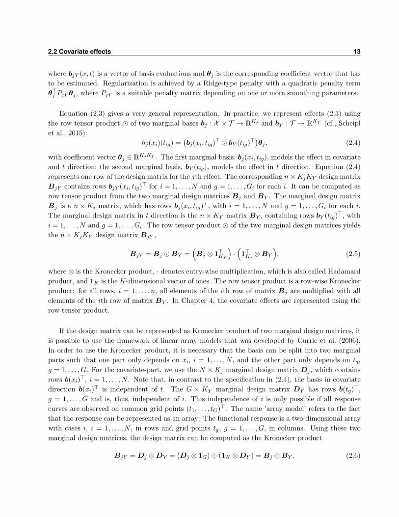
where bjY (x, t) is a vector of basis evaluations and θj is the corresponding coefficient vector that has
to be estimated. Regularization is achieved by a Ridge-type penalty with a quadratic penalty term
θ>j PjY θj , where PjY is a suitable penalty matrix depending on one or more smoothing parameters.
Equation (2.3) gives a very general representation. In practice, we represent effects (2.3) using
the row tensor product � of two marginal bases bj : X × T → RKj and bY : T → RKY (cf., Scheipl
et al., 2015):
hj(xi)(tig) =(bj(xi, tig)
> � bY (tig)>)θj , (2.4)
with coefficient vector θj ∈ RKjKY . The first marginal basis, bj(xi, tig), models the effect in covariate
and t direction; the second marginal basis, bY (tig), models the effect in t direction. Equation (2.4)
represents one row of the design matrix for the jth effect. The corresponding n×KjKY design matrix
BjY contains rows bjY (xi, tig)> for i = 1, . . . , N and g = 1, . . . , Gi for each i. It can be computed as
row tensor product from the two marginal design matrices Bj and BY . The marginal design matrix
Bj is a n×Kj matrix, which has rows bj(xi, tig)>, with i = 1, . . . , N and g = 1, . . . , Gi for each i.
The marginal design matrix in t direction is the n×KY matrix BY , containing rows bY (tig)>, with
i = 1, . . . , N and g = 1, . . . , Gi. The row tensor product � of the two marginal design matrices yields
the n×KjKY design matrix BjY ,
BjY = Bj �BY =(Bj ⊗ 1>KY
)·(1>Kj⊗BY
), (2.5)
where ⊗ is the Kronecker product, · denotes entry-wise multiplication, which is also called Hadamard
product, and 1K is the K-dimensional vector of ones. The row tensor product is a row-wise Kronecker
product: for all rows, i = 1, . . . , n, all elements of the ith row of matrix Bj are multiplied with all
elements of the ith row of matrix BY . In Chapter 4, the covariate effects are represented using the
row tensor product.
If the design matrix can be represented as Kronecker product of two marginal design matrices, it
is possible to use the framework of linear array models that was developed by Currie et al. (2006).
In order to use the Kronecker product, it is necessary that the basis can be split into two marginal
parts such that one part only depends on xi, i = 1, . . . , N , and the other part only depends on tg,
g = 1, . . . , G. For the covariate-part, we use the N ×Kj marginal design matrix Dj , which contains
rows b(xi)>, i = 1, . . . , N . Note that, in contrast to the specification in (2.4), the basis in covariate
direction b(xi)> is independent of t. The G × KY marginal design matrix DY has rows b(tg)
>,
g = 1, . . . , G and is, thus, independent of i. This independence of i is only possible if all response
curves are observed on common grid points (t1, . . . , tG)>. The name ’array model’ refers to the fact
that the response can be represented as an array: The functional response is a two-dimensional array
with cases i, i = 1, . . . , N , in rows and grid points tg, g = 1, . . . , G, in columns. Using these two
marginal design matrices, the design matrix can be computed as the Kronecker product
BjY = Dj ⊗DY = (Dj ⊗ 1G)� (1N ⊗DY ) = Bj �BY . (2.6)
14 2. Generic framework for functional regression
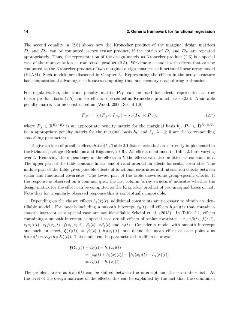
The second equality in (2.6) shows how the Kronecker product of the marginal design matrices
Dj and DY can be computed as row tensor product, if the entries of Dj and DY are repeated
appropriately. Thus, the representation of the design matrix as Kronecker product (2.6) is a special
case of the representation as row tensor product (2.5). We denote a model with effects that can be
computed as the Kronecker product of two marginal design matrices as functional linear array model
(FLAM). Such models are discussed in Chapter 3. Representing the effects in the array structure
has computational advantages as it saves computing time and memory usage during estimation.
For regularization, the same penalty matrix P jY can be used for effects represented as row
tensor product basis (2.5) and for effects represented as Kronecker product basis (2.6). A suitable
penalty matrix can be constructed as (Wood, 2006, Sec. 4.1.8)
P jY = λj(P j ⊗ IKY) + λY (IKj ⊗ P Y ), (2.7)
where P j ∈ RKj×Kj is an appropriate penalty matrix for the marginal basis bj , P Y ∈ RKY ×KY
is an appropriate penalty matrix for the marginal basis bY and λj , λY ≥ 0 are the corresponding
smoothing parameters.
To give an idea of possible effects hj(x)(t), Table 2.1 lists effects that are currently implemented in
the FDboost package (Brockhaus and Rugamer, 2016). All effects mentioned in Table 2.1 are varying
over t. Removing the dependency of the effects in t, the effects can also be fitted as constant in t.
The upper part of the table contains linear, smooth and interaction effects for scalar covariates. The
middle part of the table gives possible effects of functional covariates and interaction effects between
scalar and functional covariates. The lowest part of the table shows some group-specific effects. If
the response is observed on a common grid, the last column ’array structure’ indicates whether the
design matrix for the effect can be computed as the Kronecker product of two marginal bases or not.
Note that for irregularly observed response this is conceptually impossible.
Depending on the chosen effects hj(x)(t), additional constraints are necessary to obtain an iden-
tifiable model. For models including a smooth intercept β0(t), all effects hj(x)(t) that contain a
smooth intercept as a special case are not identifiable Scheipl et al. (2015). In Table 2.1, effects
containing a smooth intercept as special case are all effects of scalar covariates, i.e., zβ(t), f(z, t),
z1z2β(t), z1f(z2, t), f(z1, z2, t), βg(t), zβg(t) and ei(t). Consider a model with smooth intercept
and such an effect, ξ(Yi(t)) = β0(t) + hj(xi)(t), and define the mean effect at each point t as
hj(x)(t) = EX(hj(X)(t)). This model can be parametrized in different ways:
ξ(Yi(t)) = β0(t) + hj(xi)(t)
=[β0(t) + hj(x)(t)
]+[hj(xi)(t)− hj(x)(t)
]= β0(t) + hj(x)(t).
The problem arises as hj(x)(t) can be shifted between the intercept and the covariate effect. At
the level of the design matrices of the effects, this can be explained by the fact that the columns of

2.2 Covariate effects 15
Table 2.1: Overview of possible covariate effects that can be represented within the framework of functionalregression. The column ’array structure’ indicates whether the design matrix of the effect can be representedas the Kronecker product of two marginal bases in case of grid data. A similar overview table can be found inScheipl et al. (2015).
covariate(s) type of effect hj(x)(t) array
(none) smooth intercept β0(t) yesscalar covariate z linear effect zβ(t) yes
smooth effect f(z, t) yestwo scalars z1, z2 linear interaction z1z2β(t) yes
functional varying coefficient z1f(z2, t) yessmooth interaction f(z1, z2, t) yes
functional covariate x(s) linear functional effect∫S x(s)β(s, t) ds yes
scalar z and functional x(s) linear interaction z∫S x(s)β(s, t) ds yes
smooth interaction∫S x(s)β(z, s, t) ds yes
functional covariate x(s), concurrent effect x(t)β(t) no
with S = T = [T1, T2] historical effect∫ tT1x(s)β(s, t) ds no
lag effect, with lag δ > 0∫ tt−δ x(s)β(s, t) ds no
lead effect, with lead δ > 0∫ t−δT1
x(s)β(s, t) ds no
effect with t-specific integrationlimits [l(t), u(t)]
∫ u(t)l(t) x(s)β(s, t) ds no
grouping variable g group-specific smooth intercepts βg(t) yesgrouping variable g and scalar z group-specific linear effects zβg(t) yescurve indicator i curve-specific smooth residuals ei(t) yes
the design matrix BjY are linearly dependent to the columns of the design matrix of the functional
intercept. To obtain identifiable effects, Scheipl et al. (2015) propose to center those effects at each
point t. The centering is achieved by assuming that the expectation over the covariates is zero on T ,
i.e., EX(hj(X)) = 0 for all t. How to enforce those constraints is described in Appendix A.1, which is
based on Scheipl et al. (2015). Other constraints to obtain identifiable models are possible. However,
this sum-to-zero constraint for each point t yields an intuitive interpretation: the intercept can be
interpreted as global mean parameter of ξ and the covariate effects can be interpreted as deviations
from the smooth intercept. For instance, for ξ = E, β0(t) is the global mean and for ξ = median,
β0(t) is the global median.
For effects of functional covariates, a different kind of identifiability problem can arise, when the
columns of one effect BjY are linearly dependent. This can happen when the functional covariate
does not carry enough information to estimate the corresponding coefficient surface βj(s, t). Scheipl
and Greven (2016) discuss these identifiability problems and possible solutions for linear functional
effects with fixed integration limits∫S x(s)β(s, t) ds. In Section 4.2.2, we transfer their considerations
to linear functional effects with integration limits depending on t,∫ u(t)l(t) x(s)β(s, t) ds. Centering the
functional covariate by subtracting its mean function is unrelated to identifiability and yields the
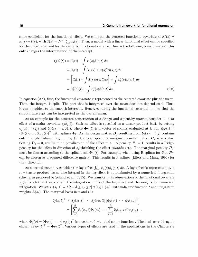
16 2. Generic framework for functional regression
same coefficient for the functional effect. We compute the centered functional covariate as x∗i (s) =
xi(s)− x(s), with x(s) = N−1∑
i xi(s). Then, a model with a linear functional effect can be specified
for the uncentered and for the centered functional variable. Due to the following transformation, this
only changes the interpretation of the intercept:
ξ(Yi(t)) = β0(t) +
∫xi(s)β(s, t) ds
= β0(t) +
∫[x∗i (s) + x(s)]β(s, t) ds
=
[β0(t) +
∫x(s)β(s, t)ds
]+
∫x∗i (s)β(s, t) ds
= β∗0(s)(t) +
∫x∗i (s)β(s, t) ds. (2.8)
In equation (2.8), first, the functional covariate is represented as the centered covariate plus the mean,
Then, the integral is split. The part that is integrated over the mean does not depend on i. Thus,
it can be added to the smooth intercept. Hence, centering the functional covariate implies that the
smooth intercept can be interpreted as the overall mean.
As an example for the concrete construction of a design and a penalty matrix, consider a linear
effect of a scalar covariate zjβj(t). Such an effect is specified as a tensor product basis by setting
bj(x) = (zj) and bY (t) = ΦY (t), where ΦY (t) is a vector of splines evaluated at t, i.e., ΦY (t) =
(Φ1(t), . . . ,ΦKY(t))> with splines Φk. As the design matrix Bj resulting from bj(x) = (zj) contains
only a single column (z1j , . . . , zNj)>, the corresponding marginal penalty matrix P j is a scalar.
Setting P j = 0, results in no penalization of the effect in zj . A penalty P j = 1, results in a Ridge-
penalty for the effect in direction of zj shrinking the effect towards zero. The marginal penalty P Y
must be chosen according to the spline basis ΦY (t). For example, when using B-splines for ΦY , P Y
can be chosen as a squared difference matrix. This results in P-splines (Eilers and Marx, 1996) for
the t direction.
As a second example, consider the lag effect∫ tt−δ xj(s)βj(s, t) ds. A lag effect is represented by a
row tensor product basis. The integral in the lag effect is approximated by a numerical integration
scheme, as proposed by Scheipl et al. (2015). We transform the observations of the functional covariate
xj(sr) such that they contain the integration limits of the lag effect and the weights for numerical
integration. We set xj(sr, t) = I [t− δ ≤ sr ≤ t] ∆(sr)xj(sr), with indicator function I and integration
weights ∆(sr). The marginal basis in x and t is
bj(x, t)> ≈ [xj(s1, t) · · · xj(sR, t)] [Φj(s1) · · · Φj(sR)]>
=
[R∑r=1
xj(sr, t)Φ1(sr) · · ·R∑r=1
xj(sr, t)ΦKj (sr)
],
where Φj(s) = (Φ1(s) · · · ΦKj (s))> is a vector of evaluated spline functions. The basis over t is again
chosen as bY (t)> = ΦY (t)>. Various types of effects are used in the applications in the Chapters 3
2.3 Transformation and loss functions 17
to 5. More details on the representation of the effects are given in the corresponding sections, as we
think that concrete applications improve the readability of the technical details.
2.3 Transformation and loss functions
The estimation problem for fitting model (2.1) is represented by using an adequate loss function. The
loss is chosen such that the transformation function is the minimizer. The model h is an element
of the set H, where H is the set of all functions from (X × T ) to L2(T , µ). We define the loss
function ρ : (Y × X ) × H → L1(T , µ) and assume that the loss is differentiable with respect to the
second argument. Thus, the loss ρ maps the data and the model to a function over t, which gives
the discrepancy of Y (t) and h(X)(t) at each t ∈ T . Consider, for instance, the absolute error loss,
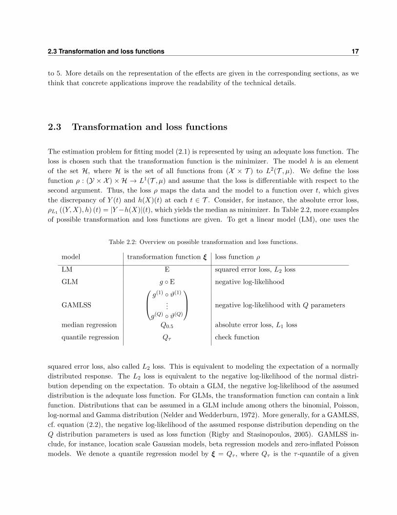
ρL1 ((Y,X), h) (t) = |Y −h(X)|(t), which yields the median as minimizer. In Table 2.2, more examples
of possible transformation and loss functions are given. To get a linear model (LM), one uses the
Table 2.2: Overview on possible transformation and loss functions.
model transformation function ξ loss function ρ
LM E squared error loss, L2 loss
GLM g ◦ E negative log-likelihood
GAMLSS
g(1) ◦ ϑ(1)
...
g(Q) ◦ ϑ(Q)
negative log-likelihood with Q parameters
median regression Q0.5 absolute error loss, L1 loss
quantile regression Qτ check function
squared error loss, also called L2 loss. This is equivalent to modeling the expectation of a normally
distributed response. The L2 loss is equivalent to the negative log-likelihood of the normal distri-
bution depending on the expectation. To obtain a GLM, the negative log-likelihood of the assumed
distribution is the adequate loss function. For GLMs, the transformation function can contain a link
function. Distributions that can be assumed in a GLM include among others the binomial, Poisson,
log-normal and Gamma distribution (Nelder and Wedderburn, 1972). More generally, for a GAMLSS,
cf. equation (2.2), the negative log-likelihood of the assumed response distribution depending on the
Q distribution parameters is used as loss function (Rigby and Stasinopoulos, 2005). GAMLSS in-
clude, for instance, location scale Gaussian models, beta regression models and zero-inflated Poisson
models. We denote a quantile regression model by ξ = Qτ , where Qτ is the τ -quantile of a given
18 2. Generic framework for functional regression
quantile τ ∈ (0, 1). To estimate a quantile regression model, the corresponding loss function is the
check function (Koenker, 2005):
ρτ (Y, h(X)) =
{(Y − h(X)) τ, if Y − h(X) ≥ 0
(Y − h(X)) (τ − 1), if Y − h(X) < 0.
For the special case of median regression, which models the 50% quantile Q0.5, the check function is
equivalent to the absolute error loss.
So far, we presented loss functions that yield the loss over the domain of the response. In order to
get a loss for each curve that is a single non-negative number, the loss is integrated over the domain
of the response T . We define the loss ` : (Y × X )×H → [0,∞) by
` ((Y,X), h) =
∫ρ((Y,X), h) dµ, (2.9)
For functional response, the integral is computed as∫T ρ ((Y,X), h) (t) dt, as µ is the Lebesgue measure
in this case. In practice, the integral is approximated by numerical integration. For scalar response,
(2.9) is equivalent to the loss function ρ, as µ is the Dirac measure in this case.
2.4 Estimation by gradient boosting
For estimation, we use a component-wise gradient boosting algorithm; see Section 1.3 for a short
introduction into boosting. Gradient boosting minimizes an expected loss criterion along the steepest
gradient descent and can thus be seen as a method of gradient descent (Breiman, 1998). The perfor-
mance of simple models, in the boosting-context called base-learners, is improved by combining them
iteratively. Component-wise boosting updates in each iteration only the best fitting base-learner.
The best fit is defined as the minimal residual sum of squares between the negative gradient and the
base-learner fit (Buhlmann and Hothorn, 2007). As each base-learner is considered separately for the
model update, it is possible to consider a large number of base-learners as potential covariate effects.
For functional regression models (2.1), each effect hj(x)(t) is represented by a base-learner. We use
for each base-learner a model as defined in (2.3) regularized by a Ridge-type penalty with penalty
matrix (2.7); see Section 2.2 for more information on the practical representation of covariate effects.
The following boosting algorithm is based on the component-wise gradient boosting algorithm of
Buhlmann and Hothorn (2007) and is described in more detail in Section 4.4. This boosting algorithm
is suitable for models that contain one linear predictor. For a GAMLSS, which models more than one
distribution parameter simultaneously, the boosting algorithm of Mayr et al. (2012) can be adapted
for functional regression models; see Section 5.4 for boosting GAMLSS with scalar response and
functional covariates.

2.4 Estimation by gradient boosting 19
Algorithm: Gradient boosting for functional regression models
Step 1: Define the bases bjY (x, t) and penalties P jY for the j = 1, . . . , J base-learners. Define the
weights wig = wi∆(tig) for all observation points i = 1, . . . , N , g = 1, . . . , Gi, where wi are
resampling weights and ∆(tig) are weights for numerical integration. Initialize the parameters
θ[0]j . Select the step-length ν ∈ (0, 1) and the stopping iteration mstop. Set the number of
boosting iterations to zero, m := 0.
Step 2: Compute the negative gradient of the empirical risk
ui(tig) := − ∂
∂hρ ((yi, xi), h) (tig)
∣∣∣∣h=h[m]
,
with h[m](xi)(tig) =∑J
j=1 bjY (xi, tig)>θ
[m]j .
Fit the base-learners for j = 1, . . . , J :
γj = arg minγ∈RKjKY
N∑i=1
Gi∑g=1
wig
{ui(tig)− bjY (xi, tig)
>γ}2
+ γ>P jY γ,
with weights wig and penalty matrices P jY .
Select the best fitting base-learner according to a least squares criterion:
j? = arg minj=1,...,J
N∑i=1
Gi∑g=1
wig
{ui(tig)− bjY (xi, tig)
>γj
}2
Step 3: Update the parameters θ[m+1]j? = θ
[m]j? + νγj? and keep all other parameters fixed, i.e.,
θ[m+1]j = θ
[m]j , for j 6= j?.
Step 4: Unless m = mstop, increase m by one and go back to step 2.
The final model is the sum of the selected base-learners: ξ(Yi|Xi = xi) =∑
j h[mstop]j (xi). All coeffi-
cients are initialized as zero, expect for the smooth intercept that is initialized by a smooth offset. For
a fair model selection, the degrees of freedom (df) must be equal for all base-learners (Kneib et al.,
2009; Hofner et al., 2011). Otherwise, the selection of base-learners in the boosting steps is biased
towards more flexible base-learners with higher df as they are more likely to yield larger improvements
of the fit. Equal numbers for the df are achieved by computing adequate smoothing parameters for
the penalty matrices. The number of df that can be given to a base-learner have an upper and a
lower bound. The minimal possible number of df is given by the rank of the null space of the penalty.
The maximal possible number of df is the number of columns of the design matrix. In order to obtain
weak learners, the df are usually chosen rather small (Kneib et al., 2009). The base-learners adapt to
the complexity of the data by the number of boosting iterations (Buhlmann and Yu, 2003). For fixed
small step-length ν, e.g., ν = 0.1, and fixed df, the number of boosting iterations is used as tuning

20 2. Generic framework for functional regression
parameter (see, e.g., Friedman, 2001). We choose the optimal stopping iteration by resampling meth-
ods such as cross-validation or bootstrapping (see, e.g., Buhlmann and Hothorn, 2007). Generally,
resampling happens on the level of independent observations. For functional response, this implies
that the resampling has to be done on the level of whole curves.
To refine the model selection, stability selection can be used in combination with component-
wise gradient boosting (Hofner et al., 2015a). Stability selection was introduced by Meinshausen
and Buhlmann (2010) and is a procedure to select influential variables with error control. Shah
and Samworth (2013) proposed complementary pairs stability selection which improves the original
selection procedure.
Boosting functional regression models is implemented in the R add-on package FDboost (Brockhaus
and Rugamer, 2016). This package is based on the fitting machine of the R package mboost (Hothorn
et al., 2016). For fitting functional GAMLSS, FDboost relies on the R package gamboostLSS (Hofner
et al., 2015b).
2.5 Comparison with existing frameworks
Using a mixed models representation, Scheipl et al. (2015) propose a functional regression framework
called ’functional additive mixed models’ (FAMMs). Within this framework, linear mixed models
for functional response can be estimated and a great variety of covariate effects are feasible. Scheipl
et al. (2016) generalize this model class to response distributions from the exponential family as well
as from other distribution families like the Negative Binomial, Beta- or t-distribution and call this
new model class ’generalized functional additive mixed models’ (GFAMMs). This framework as well
as the proposed framework based on boosting, directly model the observed data without applying a
basis transformation. Both frameworks are suited for functional data with smooth underlying curves.
The mixed models based framework is implemented in the R add-on package refund (Huang et al.,
2016).
Instead of directly modeling the functional response, a basis representation can be applied prior to
the model fit. Morris and Carroll (2006) and Meyer et al. (2015) developed a Bayesian wavelet-based
functional mixed models (WFMM) methodology. They represent functional variables by wavelets or
by other basis functions such as functional principal components (FPCs). Thus, the data is projected
into the coefficient space of the chosen basis and the regression is conducted within this space. When
using wavelets, this framework is especially suited for spiky functional data. An implementation in
Matlab is available in the software package WFMM (Herrick, 2015). Table 2.3 gives an overview on
the characteristics of the three different frameworks for regression with functional data: the newly
presented framework with array and non-array models estimated by boosting (FDboost), GFAMM
by Scheipl et al. (2015, 2016) and WFMM by Morris and Carroll (2006) and Meyer et al. (2015).
For the modeled feature of the conditional response distribution, the regression framework based
on boosting provides more flexibility than the other two frameworks. In all three regression frame-
works, a variety of covariate effects can be specified; for instance, linear and smooth effects of scalar
covariates as well as linear functional effects. FDboost is the only framework that treats a scalar
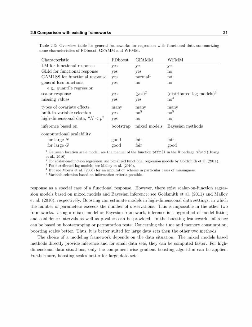
2.5 Comparison with existing frameworks 21
Table 2.3: Overview table for general frameworks for regression with functional data summarizingsome characteristics of FDboost, GFAMM and WFMM.
Characteristic FDboost GFAMM WFMM
LM for functional response yes yes yesGLM for functional response yes yes noGAMLSS for functional response yes normal1 nogeneral loss functions, yes no no
e.g., quantile regressionscalar response yes (yes)2 (distributed lag models)3
missing values yes yes no4
types of covariate effects many many manybuilt-in variable selection yes no5 no5
high-dimensional data, “N < p” yes no no
inference based on bootstrap mixed models Bayesian methods
computational scalabilityfor large N good fair fairfor large G good fair good
1 Gaussian location scale model; see the manual of the function pffr() in the R package refund (Huanget al., 2016).2 For scalar-on-function regression, see penalized functional regression models by Goldsmith et al. (2011).3 For distributed lag models, see Malloy et al. (2010).4 But see Morris et al. (2006) for an imputation scheme in particular cases of missingness.5 Variable selection based on information criteria possible.
response as a special case of a functional response. However, there exist scalar-on-function regres-
sion models based on mixed models and Bayesian inference; see Goldsmith et al. (2011) and Malloy
et al. (2010), respectively. Boosting can estimate models in high-dimensional data settings, in which
the number of parameters exceeds the number of observations. This is impossible in the other two
frameworks. Using a mixed model or Bayesian framework, inference is a byproduct of model fitting
and confidence intervals as well as p-values can be provided. In the boosting framework, inference
can be based on bootstrapping or permutation tests. Concerning the time and memory consumption,
boosting scales better. Thus, it is better suited for large data sets then the other two methods.
The choice of a modeling framework depends on the data situation. The mixed models based
methods directly provide inference and for small data sets, they can be computed faster. For high-
dimensional data situations, only the component-wise gradient boosting algorithm can be applied.
Furthermore, boosting scales better for large data sets.

22 2. Generic framework for functional regression
Chapter 3
The functional linear array model
Contributing manuscript
This chapter is based on the following paper:
Brockhaus, S., Scheipl, F., Hothorn, T., and Greven, S. (2015): The functional linear
array model. Statistical Modelling, 15(3), 279–300.
This is joint work with Fabian Scheipl (Department of Statistics, LMU Munich, Germany), Torsten
Hothorn (Epidemiology, Biostatistics and Prevention Institute, University of Zurich, Switzerland)
and Sonja Greven (Department of Statistics, LMU Munich, Germany). Fabian Scheipl had the idea
to use array models for functional response and base the estimation on gradient boosting, as in
Hothorn et al. (2013). The concrete modeling framework was mainly developed by Sarah Brockhaus
in cooperation with Sonja Greven. Torsten Hothorn pushed towards a general modeling framework
and notation style and wrote a first version of the main wrapper function FDboost() for the FDboost
package. Sarah Brockhaus implemented the R package for boosting functional regression models,
FDboost, which is based on the mboost package. Fabian Scheipl advised on R programming in general
and also in particular on the implementation of FDboost. Sarah Brockhaus conducted the simulation
study and performed the data analysis. The manuscript was written by Sarah Brockhaus under the
supervision of the other three authors. All authors were involved in proofreading the manuscript.
Chapter 3 is comprised of Brockhaus et al. (2015b) with the additional Section 3.6.3 (Canadian
weather data), which can be found in the web appendix of the article. For the thesis, the simulation
study and the applications were rerun using more recent software versions. A small simulation that
compares the computation times for boosting a FLAM with and without making use of the array
structure is added in the thesis; see Figure 3.2 in Section 3.5. The other sections of Chapter 3 match
Brockhaus et al. (2015b) except for small changes and additions in the text.
Preliminary work on Chapter 3 can be found in the conference proceedings of IWSM 2014 (29th
International Workshop on Statistical Modelling), see Brockhaus et al. (2014).

24 3. The functional linear array model
Software
The analyses within this chapter were conducted using R version 3.2.3 (R Core Team, 2015). For
boosting functional regression models, FDboost 0.2-0 (Brockhaus and Rugamer, 2016) with mboost
2.6-0 (Hothorn et al., 2016) was used. Functional regression models based on mixed models were
fitted by the R add-on package refund 0.1-14 (Huang et al., 2016).
3.1 Introduction
Functional data analysis (e.g., Ramsay and Silverman, 2005; Ferraty and Vieu, 2006) aims at analyzing
data where the observation units are functions. Often functional regression models (Ramsay and
Silverman, 2005) are of interest, i.e., models containing a functional response or at least one functional
covariate, resulting in three types of functional regression models: scalar-on-function, function-on-
scalar and function-on-function regression models. We introduce the Functional Linear Array Model
(FLAM), which includes all three model types as special cases and provides a unified model class for
functional regression. Compared to existing work, which typically focused on one of the three cases,
we provide three novel extensions. First, the use of general loss functions allows us to model not
only the conditional mean but also the median, any quantile or any other property of the conditional
distribution representable by a suitable loss function. Most existing work has focused on mean
regression for functional data, but more general loss functions than the squared error loss are in
particular important for robust regression models, using e.g., the absolute error loss or the Huber
loss, and for non-normal functional data. Second, our approach is able to handle a large number of
covariate effects –even more than observations– and model selection. Both, large numbers of variables
and variable selection are largely unaddressed in the functional data context to date. Third, we provide
a common software platform for functional regression which makes use of the array structure of FLAMs
to obtain computational efficiency for estimation via generalized linear array models (Currie et al.,
2006). Although we assume for the FLAM that the functions are intrinsically smooth and measured
on a fine grid, missing values are allowed and make estimation for sparse functional data possible,
albeit at some loss of computational efficiency. In addition to computational efficiency, this unified
and modular platform has the advantage of allowing for and encouraging extensions of the model
class (even though many models of common interest are already implemented) and new model terms
or loss functions will then be instantly available for all models covered by our framework.
A recent overview on functional regression can be found in Morris (2015). Most prior work in
this area has focused on quite narrow classes of models. The proposed models are often restricted
to one functional predictor without consideration of further scalar or functional covariates and mini-
mization of a quadratic loss function. Much work has concentrated on scalar-on-function regression
–also called signal regression– modeling the functional effect linearly as the scalar product of the
functional predictor and a smooth coefficient function, in the context of linear models (e.g., Reiss and
Ogden, 2007; James et al., 2009), generalized linear models (e.g., Marx and Eilers, 1999; Muller and
Stadtmuller, 2005; Wood, 2011; Gertheiss et al., 2013), or quantile regression models (e.g., Cardot
3.1 Introduction 25
et al., 2005; Chen and Muller, 2012a). Some approaches model the effect of the functional predictor
without the assumption of linearity (e.g., James and Silverman, 2005; Muller et al., 2013; McLean
et al., 2014; Zhu et al., 2014). A fundamentally different approach is pursued by Ferraty et al. (2005,
2007) who estimate scalar-on-function regression models nonparametrically using kernel methods,
yielding predictions but no interpretable models.
For function-on-scalar regression, which can also be viewed as smooth repeated measures varying-
coefficient models, most approaches model the conditional mean of a functional variable in the setting
of independent (e.g., Reiss et al., 2010) or dependent data (e.g., Morris and Carroll, 2006; Di et al.,
2009; Greven et al., 2010; Chen and Muller, 2012b). Staicu et al. (2012) model conditional quantiles
of a functional variable as depending on the index of the response but not on covariates.
In the context of function-on-function regression, a linear effect of a functional covariate is modeled
using a bivariate coefficient surface (e.g., Ramsay and Dalzell, 1991; Yao et al., 2005b; Ivanescu et al.,
2015). Ferraty et al. (2012) investigate a nonparametric kernel approach and Muller and Yao (2008)
consider a non-linear effect of a functional covariate
Among the most general frameworks for functional regression models are two frameworks that can
deal with functional and scalar responses and the effects of several functional and scalar covariates.
One pursues a Bayesian wavelet based approach for functional regression models; see Malloy et al.
(2010) for scalar responses in a distributed lag model and Morris and Carroll (2006), Zhu et al. (2011),
Meyer et al. (2015) for functional responses. Zhu et al. (2011) develop a robust function-on-scalar
regression model for dependent data as generalization of the model in Morris and Carroll (2006). Zhu
et al. (2011) and Meyer et al. (2015) also discuss possible generalizations to other projections than
wavelets. A second general framework estimates functional regression models based on additive mixed
models. This approach was proposed by Goldsmith et al. (2011) for scalar responses and by Ivanescu
et al. (2015) and Scheipl et al. (2015) for functional responses. Both frameworks allow random
effects, scalar and functional covariates. While our framework incorporates very similar covariate
effect types as these two approaches, it is the first to go beyond modeling the conditional mean and
to be able to deal with a large number of covariates as well as variable selection. In particular, this
means that we can estimate, e.g., quantile or expectile regression models, which is impossible in the
other two approaches focusing on generalized regression models. In addition, we can accommodate
situations with more covariates than observations. Furthermore, the efficient array methods we use for
estimation give a clear computational advantage over Scheipl et al. (2015) for increasing sample size
and number of grid points per function. Another advantage of our general framework is the unified
treatment of scalar and functional response models in both models and software, making it easier
for new users to get familiar with both within one framework, and allowing for simpler extension of
models and accompanying code for both settings simultaneously.
Our implementation of FLAMs is based on a component-wise boosting algorithm. Boosting is an
ensemble method that aims at optimizing a risk function by stepwise updates of the parameters of the
best-fitting effect in each iteration. Every effect is represented using a so called base-learner, which
is a simple model; see for instance Buhlmann and Hothorn (2007) for an introduction to boosting
algorithms in a statistical context. We derive an appropriate loss function for functional responses
26 3. The functional linear array model
based on existing loss functions for scalar responses. Boosting has some desirable properties. It can
handle many covariates of mixed types including categorical and metric scalar variables and their
interactions in mixed specifications, as for instance linear, smooth and multi-dimensional effects.
Additionally, we implement a base-learner for effects of functional covariates that can be combined
with existing base-learners to form interaction effects of functional and scalar covariates. The
number of covariates can exceed the number of observations and the covariates can be correlated. It
is of large practical importance to note that boosting can also perform variable and model selection.
Little work has been done to date on variable selection in functional regression models. Gertheiss
et al. (2013) pursued variable selection in a scalar-on-function setting. Boosting was used before in
functional data analysis to estimate particular regression models. In a setting with scalar response
and a single functional covariate, boosting was used for classification of a binary response (Kramer,
2006), for prediction of a continuous response based on kernel regression (Ferraty and Vieu, 2009)
and for feature extraction (Tutz and Gertheiss, 2010). In the context of function-on-scalar regression
Sexton and Laake (2012) used boosted regression trees. A drawback of boosting is its lack of formal
inference, which we address by bootstrapping.
In the following, we define the general FLAM and the tensor product basis representation of
the effects (Section 3.2). In order to fit a FLAM, we define a suitable loss for functional data
(Section 3.3). We give details on the estimation using a boosting algorithm in Section 3.4. In
Section 3.5, we present empirical results on simulated data to demonstrate correctness of our
software implementation and provide a comparison with functional additive mixed models (FAMM)
by Scheipl et al. (2015). The section on applications (Section 3.6) is divided into three parts for
the three cases of functional regression models. We analyze data on the viscosity of resin over time
depending on five experimental factors, where the aim is to control the hardening process. In a
function-on-scalar regression model for the viscosity we use median regression incorporating variable
selection. In the second application, spectrography data of fossil fuel samples are used to predict
their calorific values using two spectral measurements (scalar-on-function regression). We use the
well-known Canadian weather data as an example for function-on-function regression and consider
a model for precipitation curves depending on temperature curves and climatic zones, incorporating
smooth spatially correlated residuals. All analyses are fully reproducible as the datasets and the code
of the simulation and the applications are part of the online supplement or the R add-on package
FDboost and R is open-source software. The chapter concludes with a discussion in Section 3.7.
3.2 Model specification
In the following, we consider data (Y,X) taking values in Y ×X , where Y is a suitable space for the
response Y and X is a product space of suitable spaces for the covariates. Let Y be the space of
square integrable functions L2(T , µ). For functional response, the domain T is an interval over the
real numbers, T = [T1, T2], with T1, T2 ∈ R, and µ is the Lebesgue measure. For scalar response,
the set T consists of a single point, T = [T, T ], and µ is the Dirac measure. The spaces in X

3.2 Model specification 27
are defined analogously for scalar and functional covariates. We assume that Y given X follows a
conditional distribution FY |X ; the explanatory variables X may be fixed or random. As generic model
we establish the following structured additive regression model:
ξ(Y |X = x) = h(x) =J∑j=1
hj(x), (3.1)
where ξ is some transformation function, for instance the expectation, the median or some quantile.
For a generalized linear model, the transformation function corresponds to the expectation composed
with the link function g that connects response and linear predictor, i.e., ξ = g ◦ E. The linear
predictor h is the sum of partial effects hj which implies additivity. Note, however, that a partial
effect hj can depend on more than one covariate allowing, e.g., for interactions. Each effect hj(x) ∈ Yis a real-valued function. To give an overview of effects hj(x) that can be specified within the proposed
framework, Table 3.1 lists the effects that are currently implemented in the FDboost package. In order
to obtain identifiable models, further constraints on the hj are necessary. For an intercept β0 in the
model, we center all effects hj , that contain an intercept as a special case, by assuming that the
expectation over the covariates is zero on T , i.e. EX(hj(X)) ≡ 0. We describe these constraints and
how to include them in the array framework in Appendix A.1.
Table 3.1: Basic effects that can be fitted within a FLAM. A similar overview table is given in Scheipl et al.(2015).
covariate(s) type of effect hj(x)(t)
(none) smooth intercept β0(t)scalar covariate z linear effect zβ(t)
smooth effect f(z, t)two scalars z1, z2 linear interaction z1z2β(t)
functional varying coefficient z1f(z2, t)smooth interaction f(z1, z2, t)
functional covariate x(s) linear functional effect∫x(s)β(s, t) ds
scalar z and functional x(s) linear interaction z∫x(s)β(s, t) ds
smooth interaction∫x(s)β(z, s, t) ds
grouping variable g group-specific intercepts βg(t)grouping variable g and scalar z group-specific linear effects zβg(t)curve indicator i curve-specific smooth residuals ei(t)
Each effect hj(x) is represented using a tensor product basis
hj(x)(t) =(bj(x)> ⊗ bY (t)>
)θj , (3.2)
where ⊗ is the Kronecker product, bj : X → RKj is a vector of basis functions depending on one or
several covariates, bY : T → RKY is a vector of basis functions over the domain of the response and
θj ∈ RKjKY is a vector of coefficients. In the case of scalar-on-function regression, bY (t) ≡ 1 with
28 3. The functional linear array model
KY = 1. Regularization of the effects is achieved by a quadratic penalty term. A suitable penalty
matrix for a tensor product basis as in equation (3.2) can be constructed as P jY = λj(P j ⊗ IKY) +
λY (IKj ⊗ P Y ), where P j ∈ RKj×Kj is an appropriate penalty matrix for the marginal basis bj(xi),
P Y ∈ RKY ×KY is an appropriate penalty matrix for the marginal basis bY (t), and λj , λY ≥ 0 are the
corresponding smoothing parameters (Wood, 2006, Sec. 4.1.8). Other penalty matrices are possible,
e.g., the direct Kronecker product of the two marginal penalties P ∗jY = λjP j⊗P Y (Wood, 2006, Sec.
4.1.8) or the penalty of the sandwich-smoother P ∗∗jY = λjP j⊗B>YBY +λYB>j Bj⊗P Y +λjλY P j⊗P Y ,
where Bj and BY are the design matrices of the marginal bases (Xiao et al., 2013). The penalty
term has a quadratic form, resulting in a Ridge-type penalty. The description of bases and suitable
penalty matrices corresponding to the effects hj(x) in Table 3.1 are deferred to Section 3.6, as we
hope that concrete examples improve readability of these technical details. The three examples in
Section 3.6 are chosen in particular such that bases and penalties for most effect types in Table 3.1
are introduced.
As we represent all effects as Kronecker products of two bases and use a Ridge-type penalty, the
model is a special case of a generalized linear array model as introduced by Currie et al. (2006). This
approach in particular avoids rearranging responses and coefficients into vectors, but preserves the
array structure throughout and makes use of the special Kronecker structure in the design matrix to
reduce computations to nested operations in lower dimensions. For instance, it is not necessary to
actually compute and save the NG × KjKY design matrix, where N is the number of observation
units and G is the number of observation points per functional response. Instead we only need to
compute and save the much smaller marginal basis matrices. By defining suitable array-based linear
algebra routines the number of operations required to compute effect estimates and predictions, as
well as the storage requirements, are reduced dramatically, cf. Currie et al. (2006).
3.3 Estimation
The basic idea for the estimation of a FLAM (3.1) is the use of an adequate loss function that
represents the estimation problem. The choice of the loss function depends on the transformation
function ξ and on the conditional distribution of the response. In the following, we present some
possible loss functions to give an idea of the variety of models that can be represented within this
framework. Let ρ : (Y × X ) ×H → L1(T , µ) be a function mapping the data (Y,X) and the model
h to a function in the space of integrable functions L1(T , µ). The model h is an element of the set
H = (L2(T , µ))(X×T ), which is the set of all functions from (X × T ) to L2(T , µ). In other words, ρ
maps the data and the model to a function over the domain of the response which computes a measure
of discrepancy between Y (t) and h(X)(t) for each t ∈ T . For clarity, the argument t is omitted in
the following examples of loss functions. For a continuous Y , a typical choice is the squared error
loss, the so called L2 loss, ρL2 ((Y,X), h) = 12(Y −h(X))2. Minimizing the quadratic loss corresponds
to least squares optimization and is equivalent to minimizing the negative log-likelihood of a normal
distribution. Thus minimizing the L2 loss yields the classical linear regression model for conditionally

3.4 Estimation by gradient boosting 29
normally distributed response and corresponds to the case when the transformation function is the
expectation.
One possibility to obtain a more robust model is to use the absolute loss, also called L1 loss, which
is equivalent to minimizing the negative log-likelihood of the Laplace distribution and is defined
as ρL1 ((Y,X), h) = |Y − h(X)|. The L1 loss is minimized by the conditional median and hence
corresponds to median regression. To obtain quantile regression, i.e. ξ(Y |X) = Qτ (Y |X), where
Qτ (Y |X) is the τ -quantile of Y conditional on X for a given quantile τ ∈ (0, 1), one can use the check
function (Koenker, 2005)
ρτ ((Y,X), h) =
{(Y − h(X))τ, if Y − h(X) ≥ 0
(Y − h(X))(τ − 1), if Y − h(X) < 0,
which is minimized by the τ -quantile. Modeling quantiles is a distribution-free approach and is often
of interest for skewed and heteroskedastic conditional distributions or in applications where some
extreme quantile is of special interest.
If it is assumed that the conditional distribution of the response is from the exponential family,
the negative log-likelihood is an appropriate loss function. Examples for exponential family distribu-
tions used for generalized linear models (GLMs) include binomial, Poisson, log-normal and Gamma
distributions (Nelder and Wedderburn, 1972).
We define the loss function ` : (Y × X )×H → R that results in a real-valued loss by integrating
the loss function ρ
` ((Y,X), h) =
∫ρ((Y,X), h) dµ. (3.3)
Remember that µ is the Dirac measure for scalar response and the Lebesgue measure for functional
response. Weight functions can be incorporated by defining dµ(t) = v(t)dt where v(t) > 0 for t ∈ Tand v(t) = 0 for t 6∈ T , e.g., v(t) = I(t ∈ T ), with I the indicator function. Weight functions that
are not constant can be used in the case that a certain area of T is of special interest or variability
varies along T .
3.4 Estimation by gradient boosting
The FLAM (3.1) could be fitted using different approaches, e.g., by penalized likelihood-based meth-
ods or Bayesian methods, replacing penalties with priors. We chose to use boosting as it can easily
deal with both the diversity of possible loss functions of interest as well as with a large number of co-
variates (potentially more than observations) and variable selection. Boosting is an ensemble method
that pursues a divide-and-conquer strategy for optimizing an expected loss criterion. The estimator
is updated step-by-step to minimize the loss criterion ` as defined in (3.3) along the steepest gradient
descent. The model is represented as the sum of simple (penalized) regression models, the so called
base-learners, that fit the negative gradient in each step (Friedman, 2001; Buhlmann and Hothorn,
2007). The base-learners determine the type of possible covariate effects. Their parametrization for
30 3. The functional linear array model
the FLAM (3.1) was given in equation (3.2). The loss criterion determines which characteristic of the
response variable’s conditional distribution is the goal of optimization. The loss function is assumed
to be differentiable with respect to h. The aim of boosting is to find the solution of the optimization
problem
h∗ = arg minh
EY,X ` ((Y,X), h) . (3.4)
In practical problems the expectation in (3.4) has to be replaced by the observed mean and the integral
in (3.3) has to be approximated by the weighted sum over the observed points, giving optimization
of the empirical risk. We consider a random sample (Yi, Xi), i = 1, . . . , N , where Yi ∼ FY |Xifollow
a common distribution and Xi can be fixed or random. We assume that the response Yi is observed
over a common grid (t1, . . . , tG) ∈ T . Then we use the empirical risk for optimization
h∗ = arg minh
(GN)−1N∑i=1
G∑g=1
wi∆i(tg)ρ ((Yi, Xi), h) (tg),
where wi are weights for the observations and ∆i(tg) are integration weights. The weights wi are
used in resampling methods, e.g., bootstrapping or subsampling, and are set to one for an ordinary
model fit. The integration weights ∆i(tg) are weights of a numerical integration scheme. As a default,
Riemann sums are used. In the case of a missing value Yi′(tg′), the corresponding weight ∆i′(tg′) is
set to zero and the integration weights of adjacent observations ∆i′(tg′−1), ∆i′(tg′+1) are increased
accordingly. If µ includes a weight function, the integration weights are pre-multiplied by v(tg) at
each tg.
We adapt the component-wise gradient boosting algorithm developed by Hothorn et al. (2013) to
estimate conditional transformation models for the case of functional regression models. In detail, we
use the following algorithm to estimate FLAMs (3.1).
Algorithm: Gradient boosting for FLAMs
Step 1: Define the bases bj(x), bY (t), with penalties P jY , for the j = 1, . . . , J base-learners. Define
the weights wig = wi∆i(tg), i = 1, . . . , N , g = 1, . . . , G for the observations. Initialize the
parameters θ[0]j for j = 1, . . . , J . Select the step-length ν ∈ (0, 1) and the stopping iteration
mstop. Set the number of boosting iterations to zero, m := 0.
Step 2: Compute the negative gradient of the empirical risk
ui(tg) := − ∂
∂hρ((yi, xi), h)(tg)
∣∣∣∣h=h[m]
,

3.4 Estimation by gradient boosting 31
with h[m](xi)(tg) =∑J
j=1
(bj(xi)
> ⊗ bY (tg)>)θ[m]
j .
Fit the j = 1, . . . , J base-learners:
γj = arg minγ∈RKjKY
N∑i=1
G∑g=1
wig
{ui(tg)−
(bj(xi)
> ⊗ bY (tg)>)γ}2
+ γ>P jY γ,
with weights wig and penalty matrices P jY .
Select the best base-learner:
j? = arg minj=1,...,J
N∑i=1
G∑g=1
wig
{ui(tg)−
(bj(xi)
> ⊗ bY (tg)>)γj
}2.
Step 3: Update the parameters θ[m+1]j? = θ
[m]j? + νγj? and keep all other parameters fixed, i.e.,
θ[m+1]j = θ
[m]j , for j 6= j?.
Step 4: Unless m = mstop, increase m by one and go back to step 2.
Then the final model is:
ξ(Yi|Xi = xi) =
J∑j=1
h[mstop]j (xi),
with h[mstop]j (xi)(t) =
(bj(xi)
> ⊗ bY (t)>)θ
[mstop]j .
To complete the specification of the boosting algorithm, it is necessary to set all parameters
mentioned in step 1. The bases and their corresponding penalty matrices directly correspond to the
chosen partial effects hj(x) in the model, with an overview of possible model terms given in Table 3.1
and various examples of choices for bases and penalties discussed in Section 3.6. Obvious choices are
splines for smooth terms and the observations themselves for linear terms, in each case provided with
adequate penalty matrices. We used a simplified penalty matrix P jY = λj(P j ⊗ IKY+ IKj ⊗ P Y )
which contains only one smoothing parameter for both directions in our implementation. Additional
simulations (results not shown) indicate that the effect estimates still adapt well to anisotropic effect
surfaces over the course of the boosting iterations. The smoothness parameters λj are chosen such that
the degrees of freedom are the same for all base-learners to ensure a fair model selection. Otherwise
base-learners with higher degrees of freedom are more likely to be chosen (Hofner et al., 2011). The
resulting estimates adapt to the true complexity of the effects by the selection frequency of the base-
learners, which depends on the number of boosting iterations mstop (Buhlmann and Yu, 2003). A
natural choice for all initial values θ[0]j is zero. However, the convergence rate of the boosting algorithm
is faster if a suitable offset is chosen for the intercept. For scalar responses, typical choices are mean
or median. For functional responses, we use a smoothed mean or median function as offset.
The number of boosting iterations mstop and the step-length ν are connected, as a smaller step-
length typically requires more boosting iterations. Choosing the step-length sufficiently small (e.g.,
ν = 0.1) and using the number of boosting iterations as tuning parameter has been shown to be a good

32 3. The functional linear array model
strategy (Friedman, 2001). Stopping early here leads to regularized effect estimates and the number of
boosting iterations mstop can be chosen by resampling methods like cross-validation or bootstrapping.
If bootstrapping is used, the weights wi are drawn from an N -dimensional multinomial distribution
with constant probability parameters pi = N−1, i = 1, . . . , N . Then the out-of-bag (OOB) empirical
risk with weights wOOBi = I(wi = 0) is computed and the stopping iteration yielding the lowest
empirical risk is chosen (Hothorn et al., 2013).
Stability selection (Meinshausen and Buhlmann, 2010) can be used to improve variable selection.
The basic idea is to fix an upper bound for the per-family-error-rate and the expected number of
terms in the model. Then the model is refitted on subsamples of the data and the stability selection
procedure provides a cutoff value for the relative frequency of a base-learner to be selected among
the first model terms across the subsamples. Terms with selection frequencies greater than the cutoff
are retained in the model. In this paper, we use complementary pairs stability selection as proposed
by Shah and Samworth (2013), which improves on the theoretical guarantees of the original proposal
of Meinshausen and Buhlmann (2010) by replacing purely random subsampling of the data with
subsampling consisting of complementary pairs; for each subsample of size bN/2c another subsample
containing the observations not used in that subsample, i.e., the complementary pair, is also used as
a training subsample. The combination of stability selection and component-wise gradient boosting
is discussed in Hofner et al. (2015a).
3.5 Simulation study
The aim of the simulation study is to demonstrate correctness of our software implementation in
the R add-on package FDboost. Details on the construction of the base-learner for a functional
covariate are given later in Section 3.6.2. Boosting for scalar responses and covariates is well tested
and extensive simulation studies have already been conducted for the R add-on package mboost
on which our implementation is based (e.g., Buhlmann and Hothorn, 2007; Schmid and Hothorn,
2008a; Fenske et al., 2011). To keep the simulation section short, we use a function-on-function
setting which covers the functional response and the functional covariate setting–both new in
our framework–at the same time. To allow comparison with a benchmark we simulate a mean
regression model, i.e. ξ = E, with a moderate number of covariates and no need for variable
selection. We can then use functional additive mixed models (FAMM) proposed by Scheipl et al.
(2015) and implemented in the R add-on package refund as a benchmark. Scheipl et al. (2015)
demonstrated in the function-on-scalar setting that the FAMM approach is better suited to
smooth functional data–as we assume–than the Bayesian wavelet based approach by Morris and
Carroll (2006). The effect of the functional covariates in both approaches is specified using the
default settings, which means that a tensor product of cubic regression splines is used in FAMM
and cubic P-splines are used in the boosting algorithm. For the boosting algorithm of the FLAM,
the optimal mstop is determined by 10-fold bootstrap over curves and the maximal mstop is set to 2000.

3.5 Simulation study 33
Simulation setup and goodness of fit measure. We consider a model with functional response
and two functional covariates. The true model is
Yi(t) = β0(t) +
∫x1i(s)β1(s, t) ds+
∫x2i(s)β2(s, t) ds+ εit,
with s, t ∈ [0, 1]. The functional covariates are simulated using a sum of five natural cubic B-splines
with random coefficients from a uniform distribution U [−3, 3]. The smooth global intercept is β0(t) =
cos(3πt2) + 2, the coefficient function β1(s, t) is a bimodal surface β1(s, t) = φ(s, .2, .3)φ(t, .2, .3) +
φ(s, .6, .3)φ(t, .8, .25), where φ(·, µ, σ) is the density of the normal distribution with mean µ and
standard deviation σ, and the coefficient function β2(s, t) is unimodal with β2(s, t) = 1.5 sin(πt +
0.3) sin(πs). The errors are normally distributed with εit ∼ N(0, σ2ε), where σ2
ε depends on the signal-
to-noise ratio. In Appendix B.1 a figure of the true coefficient functions and responses together with
the estimates by FAMM and FLAM is given for an exemplary setting. We consider all combinations
of the following parameter settings:
1. Total number of observations N ∈ {100, 500}.
2. Number of grid points G ∈ {30, 100}; the same number of grid points is used for response and
functional covariates.
3. Signal-to-noise ratio SNRε ∈ {1, 2}, where SNRε is the ratio of the standard deviation of the
linear predictor and the standard deviation of the residuals.
We run ten replications per combination of parameter settings, which results in narrow interquartile
ranges of the performance measures and thus seems sufficient. As a measure of the goodness of
estimation the relative integrated mean squared error (reliMSE) is used:
reliMSE(Y (t)) =
∑Ni=1
∫ (ηi(t)− Yi(t)
)2dt∑N
i=1
∫ (ηi(t)− Y
)2dt
where ηi(t) is the true value of the response without noise, Yi(t) is the predicted value and
Y = N−1∑
i
∫ηi(t) dt is the global mean of the response. Thus, the mean squared error (MSE)
is standardized with respect to the global variability of the response. The reliMSE is calculated
analogously for the coefficient surface β(s, t):
reliMSE(β(s, t)) =
∫∫ (β(s, t)− β(s, t)
)2dsdt∫∫ (
β(s, t)− β)2dsdt
where β(s, t) is the true coefficient surface, β(s, t) is its estimate and β =∫∫
β(s, t) dsdt is the overall
mean of the true surface. Thus the MSE is standardized by a measure of the global variability of
the coefficient surface. The reliMSE is defined analogously for the univariate coefficient function β0(t).
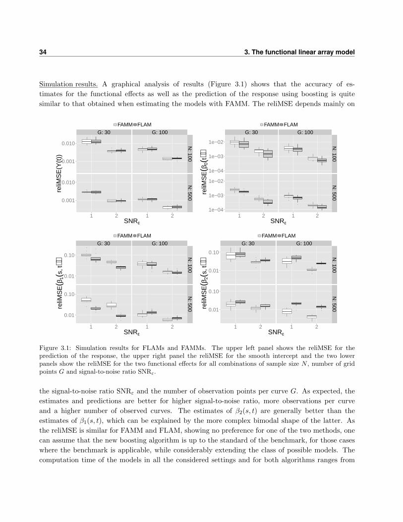
34 3. The functional linear array model
Simulation results. A graphical analysis of results (Figure 3.1) shows that the accuracy of es-
timates for the functional effects as well as the prediction of the response using boosting is quite
similar to that obtained when estimating the models with FAMM. The reliMSE depends mainly on
G: 30 G: 100
●
●
●
●
●
0.001
0.010
0.001
0.010
N: 100
N: 500
1 2 1 2SNRε
reliM
SE
(Y(t
))
FAMM FLAM
G: 30 G: 100
●
●
●●
●
●
1e−04
1e−03
1e−02
1e−04
1e−03
1e−02
N: 100
N: 500
1 2 1 2SNRε
reliM
SE
(β0(t
))
FAMM FLAM
G: 30 G: 100
●
●
●
●
●
●
●
●
●
●
●
●
●
0.01
0.10
0.01
0.10
N: 100
N: 500
1 2 1 2SNRε
reliM
SE
(β1(s
, t))
FAMM FLAM
G: 30 G: 100
●
●
●
●
●
0.01
0.10
0.01
0.10
N: 100
N: 500
1 2 1 2SNRε
reliM
SE
(β2(s
, t))
FAMM FLAM
Figure 3.1: Simulation results for FLAMs and FAMMs. The upper left panel shows the reliMSE for theprediction of the response, the upper right panel the reliMSE for the smooth intercept and the two lowerpanels show the reliMSE for the two functional effects for all combinations of sample size N , number of gridpoints G and signal-to-noise ratio SNRε.
the signal-to-noise ratio SNRε and the number of observation points per curve G. As expected, the
estimates and predictions are better for higher signal-to-noise ratio, more observations per curve
and a higher number of observed curves. The estimates of β2(s, t) are generally better than the
estimates of β1(s, t), which can be explained by the more complex bimodal shape of the latter. As
the reliMSE is similar for FAMM and FLAM, showing no preference for one of the two methods, one
can assume that the new boosting algorithm is up to the standard of the benchmark, for those cases
where the benchmark is applicable, while considerably extending the class of possible models. The
computation time of the models in all the considered settings and for both algorithms ranges from
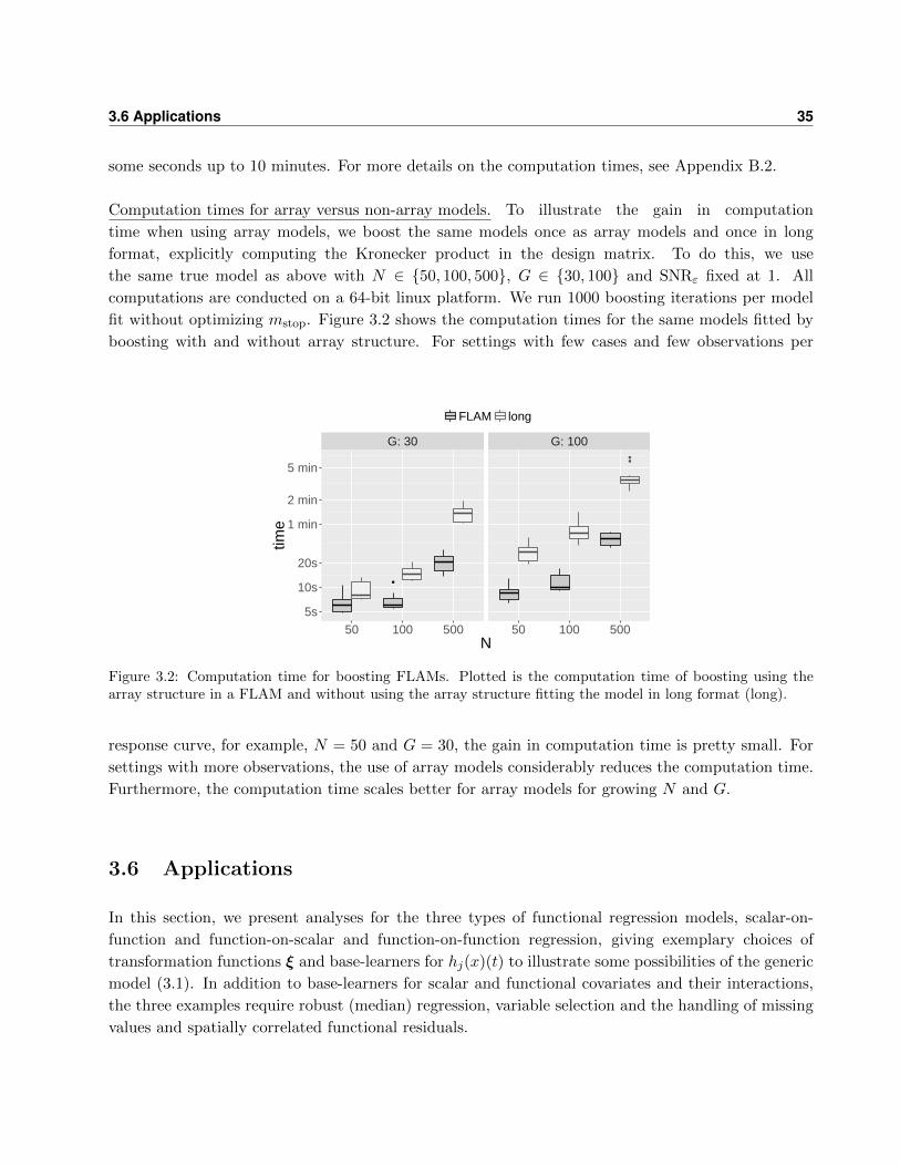
3.6 Applications 35
some seconds up to 10 minutes. For more details on the computation times, see Appendix B.2.
Computation times for array versus non-array models. To illustrate the gain in computation
time when using array models, we boost the same models once as array models and once in long
format, explicitly computing the Kronecker product in the design matrix. To do this, we use
the same true model as above with N ∈ {50, 100, 500}, G ∈ {30, 100} and SNRε fixed at 1. All
computations are conducted on a 64-bit linux platform. We run 1000 boosting iterations per model
fit without optimizing mstop. Figure 3.2 shows the computation times for the same models fitted by
boosting with and without array structure. For settings with few cases and few observations per
G: 30 G: 100
●
●
●
5s
10s
20s
1 min
2 min
5 min
50 100 500 50 100 500N
time
FLAM long
Figure 3.2: Computation time for boosting FLAMs. Plotted is the computation time of boosting using thearray structure in a FLAM and without using the array structure fitting the model in long format (long).
response curve, for example, N = 50 and G = 30, the gain in computation time is pretty small. For
settings with more observations, the use of array models considerably reduces the computation time.
Furthermore, the computation time scales better for array models for growing N and G.
3.6 Applications
In this section, we present analyses for the three types of functional regression models, scalar-on-
function and function-on-scalar and function-on-function regression, giving exemplary choices of
transformation functions ξ and base-learners for hj(x)(t) to illustrate some possibilities of the generic
model (3.1). In addition to base-learners for scalar and functional covariates and their interactions,
the three examples require robust (median) regression, variable selection and the handling of missing
values and spatially correlated functional residuals.
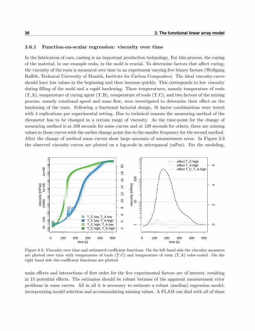
36 3. The functional linear array model
3.6.1 Function-on-scalar regression: viscosity over time
In the fabrication of cars, casting is an important production technology. For this process, the curing
of the material, in our example resin, in the mold is crucial. To determine factors that affect curing,
the viscosity of the resin is measured over time in an experiment varying five binary factors (Wolfgang
Raffelt, Technical University of Munich, Institute for Carbon Composites). The ideal viscosity-curve
should have low values in the beginning and then increase quickly. This corresponds to low viscosity
during filling of the mold and a rapid hardening. Three temperatures, namely temperature of resin
(T A), temperature of curing agent (T B), temperature of tools (T C), and two factors of the mixing
process, namely rotational speed and mass flow, were investigated to determine their effect on the
hardening of the resin. Following a fractional factorial design, 16 factor combinations were tested
with 4 replications per experimental setting. Due to technical reasons the measuring method of the
rheometer has to be changed in a certain range of viscosity. As the time-point for the change of
measuring method is at 109 seconds for some curves and at 129 seconds for others, there are missing
values in those curves with the earlier change point due to the smaller frequency for the second method.
After the change of method some curves show large amounts of measurement error. In Figure 3.3
the observed viscosity curves are plotted on a log-scale in micropascal (mPas). For the modeling,
●●●●●●●●●●●●●●●●●●●●●●●●●●●●●●●●●●●●●●●●●●●●●●●●●●●●●●●●●●●●●●●●●●●●●●●●●●●●●●●●●●●●●●●●●●●●●●●●●●
0 100 200 300 400 500time [s]
visc
osity
[mP
as]
1010
010
000
1e+
061e
+08
24
68
1012
1416
1820
T_C low, T_A lowT_C low, T_A highT_C high, T_A lowT_C high, T_A high
●●●●●●●●●●●●●●●●●●●●●●●●●●●●●●●●●●●●●●●●●●●●●●●●●●●●●●●●●●●●●●●●●●●●●●●●●●●●●●●●●●●●●●●●●●●●●●●●●●
0 100 200 300 400 500time [s]
visc
osity
[mP
as]
110
100
02
46
effect T_C higheffect T_A higheffect T_C, T_A high
Figure 3.3: Viscosity over time and estimated coefficient functions. On the left hand side the viscosity measuresare plotted over time with temperature of tools (T C) and temperature of resin (T A) color-coded. On theright hand side the coefficient functions are plotted.
main effects and interactions of first order for the five experimental factors are of interest, resulting
in 15 potential effects. The estimates should be robust because of the apparent measurement error
problems in some curves. All in all it is necessary to estimate a robust (median) regression model,
incorporating model selection and accommodating missing values. A FLAM can deal with all of these
3.6 Applications 37
problems: Median regression is obtained by using the absolute loss, variable selection is achieved by
stability selection, and missing values are dealt with by setting the corresponding weights to zero.
In a first step a smooth intercept, all main effects and all interaction terms of first order are
included in the model as smooth effects over time. To estimate such a model we need a base-learner
for an effect of the form xβ(t), where x is a dummy variable for a factor or an interaction and β(t) is
the smooth coefficient function over time. Such an effect is obtained by setting bj(x)> = (1 x) and
bY (t) = ΦY (t), where ΦY (t) is a vector of cubic B-splines evaluated at t. The smooth intercept is
represented by setting b1(x)> = (1). In order to get more stable estimates and reduce the necessary
number of boosting iterations, we include an intercept term in each base-learner. After fitting the
model, the intercept-part is subtracted from each coefficient function and added to the global intercept.
The penalty matrix P j for the linear term in the dummy variable is 0 so that the linear term is
unpenalized. The penalty matrix P Y is D>D with second order difference matrix D, yielding P-
splines for the time-varying effects (Eilers and Marx, 1996).
The optimal stopping iteration is determined by 10-fold bootstrapping over curves. In the re-
sulting model, all main effects and most of the interaction effects are selected. Most base-learners
contribute very small effects to the prediction of the viscosity and are selected quite rarely. To obtain
a parsimonious model only containing important effects we conduct complementary pairs stability se-
lection (Shah and Samworth, 2013). We set the per-family-error-rate to 2 and the expected number of
terms in the model to 5. For the 16 possible base-learners, this results in a cutoff value of 0.63. Using
a total of 100 subsamples, the effects for temperature of tools (T A), temperature of resin (T C) and
their interaction are selected into the model. When using more restrictive parameters in the stability
selection, e.g., smaller per-family-error-rate, the main effects are selected very reliably, the interaction
term is often not selected, but nevertheless has a quite high selection probability compared to the
other model terms. We thus keep these three effects in the model, yielding
median (log(visi(t))|T Ai,T Ci) = β0(t) + T AiβA(t) + T CiβC(t) + T ACiβAC(t),
where visi(t) is the viscosity of observation i at time t, T Ai and T Ci are the temperatures of
resin and of tools, respectively, each coded as -1 for the lower and 1 for the higher temperature.
The interaction T ACi is 1 if both temperatures are in the higher category and -1 otherwise. The
estimated coefficients for this model are shown in Figure 3.3 on the right hand side.
Temperature of tools (T C) has a very strong influence. For higher temperature of tools, the resin
has lower viscosity in the beginning, but from about 40 seconds onwards it is curing faster. For the
temperature of the resin (T A), the effect is similar but much smaller, i.e., the resin cures faster for
higher temperatures. If both temperatures are in the higher category the viscosity curves have the
desired shape (low in the beginning and rapid increase). The other factors seem to have no or only
a very small influence on the curing process. This is good news for the production process, as these
parameters do not have to be controlled precisely.
38 3. The functional linear array model
3.6.2 Scalar-on-function regression: spectral data of fossil fuels
In this application, the aim is to predict the heat value of fossil fuels using spectral data (Fuchs
et al., 2015, Siemens AG). The dataset was obtained in a laboratory and contains the heat value in
megajoule (MJ), percentage of humidity and two spectra types with different wavelength ranges for
129 fossil fuel samples. One spectrum is ultraviolet-visible (UV-VIS), measured at 1335 wavelengths,
in the range of 250.4 to 878.4 nanometer (nm), the other a near infrared spectrum (NIR), measured
at 2307 wavelengths, in the range of 800.4 to 2779.0nm. The observation points along the wavelength
are non-equidistant for both spectra, with larger distances for higher wavelengths.
The aim is to predict the heat value using information obtainable as measurements in a power
plant, i.e., using only the spectral data. To use more information, we compute the derivatives of
both spectra as further functional covariates. As the humidity cannot be measured automatically in
a power plant, it should not be used directly for the prediction of the heat value. But it is possible
to predict the humidity using the spectral data and then to use predicted humidity as additional
variable. To predict the humidity we use a scalar-on-function regression model with both spectra
and both derivatives as covariates. For this dataset, the humidity can be predicted quite accurately,
with the relative mean squared error (relMSE) determined by 50-fold bootstrap being about 10%.
Through the predicted humidity the information contained in the spectra is used in a non-linear way
for the model of the heat value. Figure 3.4 shows a histogram of the heat value (top left panel),
whose distribution is skewed towards higher values. The scatterplot of heat value against predicted
humidity (Figure 3.4 top right) shows that low heat values all occur for rather low humidity values,
but for the low humidity values there are high heat values as well.
For this application, we want to estimate a scalar-on-function regression model that predicts the
heat values as precisely as possible. Two spectra, their derivatives, and the predicted humidity are
available as predictors and can be used to specify models with different covariate effects. The most
complex model contains the functional effects of the two spectra and their derivatives, the effect of
the predicted humidity and the interaction effects of the predicted humidity with the four functional
variables. The functional variables are denoted by xki, k = 1, . . . , 4, and the predicted humidity by
zi, i = 1, . . . , 129. Then we can write the model as
E(Yi|xi, zi) = β0 +
4∑k=1
∫xki(sk)βk(sk) dsk + f(zi) +
4∑k=1
∫xki(sk)αk(sk, zi) dsk, (3.5)
where Yi are the heat values, βk(sk) are the coefficients of the main functional effects, sk are the
respective wavelengths, f(zi) is the smooth effect of the predicted humidity and αk(sk, zi) are the
interaction effects of the functional covariates with the predicted humidity. For the model fit, we
standardize the domain of the two spectra to [0,1].
To estimate the full model (3.5), linear effects of functional variables, a smooth effect of a scalar
variable and interactions between them are needed. The effect of a functional covariate x(s) over
the domain s ∈ S is modeled as∫S x(s)β(s) ds. The integral can be approximated numerically as a
weighted sum over (s1, . . . , sR)>, the grid of observation points in S, by using adequate integration

3.6 Applications 39
Figure 3.4: Spectral data of fossil fuels. The coloring of all plots is according to the heat value in MJ, withred meaning low heat value and yellow meaning high heat value. The histogram at the top left can be usedas a legend. The scatter plot at the top right shows the heat value depending on the predicted humidity. Thelower panel shows the UV-VIS and the NIR spectra colored according to the heat value.
weights ∆(s), yielding∫S x(s)β(s) ds ≈
∑Rr=1 ∆(sr)x(sr)β(sr) (Wood, 2011). Then we compute the
basis as
bj(x(s))> = [x(s1) · · · x(sR)]
Φj(s1)>
...
Φj(sR)>
, (3.6)
where x(s) = ∆(s)x(s) is the original observation multiplied with its integration weight and Φj(s) is a
vector of B-splines evaluated at s. The penalty matrix P j is a squared difference matrix. The smooth
effect f(zi) of the scalar covariate upon a scalar response is a standard problem and is estimated by
P-splines, i.e. bj(z) = Φj(z) with difference penalty P j . An interaction term between a functional
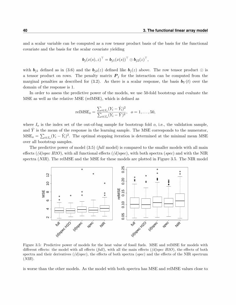
40 3. The functional linear array model
and a scalar variable can be computed as a row tensor product basis of the basis for the functional
covariate and the basis for the scalar covariate yielding
bj(x(s), z)> = bj1(x(s))> � bj2(z)>,
with bj1 defined as in (3.6) and the bj2(z) defined like bj(z) above. The row tensor product � is
a tensor product on rows. The penalty matrix P j for the interaction can be computed from the
marginal penalties as described for (3.2). As there is a scalar response, the basis bY (t) over the
domain of the response is 1.
In order to assess the predictive power of the models, we use 50-fold bootstrap and evaluate the
MSE as well as the relative MSE (relMSE), which is defined as
relMSEo =
∑i∈Io(Yi − Yi)2∑i∈Io(Yi − Y )2
, o = 1, . . . , 50,
where Io is the index set of the out-of-bag sample for bootstrap fold o, i.e., the validation sample,
and Y is the mean of the response in the learning sample. The MSE corresponds to the numerator,
MSEo =∑
i∈Io(Yi − Yi)2. The optimal stopping iteration is determined at the minimal mean MSE
over all bootstrap samples.
The predictive power of model (3.5) (full model) is compared to the smaller models with all main
effects ((d)spec H2O), with all functional effects ((d)spec), with both spectra (spec) and with the NIR
spectra (NIR). The relMSE and the MSE for these models are plotted in Figure 3.5. The NIR model
●
●
●
●
●
●
●
●
●
●
24
68
1012
MS
E
full
(d)s
pec H
2O
(d)s
pec
spec
NIR
●
●
●●
●
●●
●
●
●
●●●
●●
●●
●
●
●
●
0.05
0.10
0.15
0.20
0.25
relM
SE
full
(d)s
pec H
2O
(d)s
pec
spec
NIR
Figure 3.5: Predictive power of models for the heat value of fossil fuels. MSE and relMSE for models withdifferent effects: the model with all effects (full), with all the main effects ((d)spec H2O), the effects of bothspectra and their derivatives ((d)spec), the effects of both spectra (spec) and the effects of the NIR spectrum(NIR).
is worse than the other models. As the model with both spectra has MSE and relMSE values close to

3.6 Applications 41
those of the more complex models, we keep that model. The relMSE values of around 10% indicate
adequate prediction of the heat values. The coefficient estimates (Figure 3.6) on the entire dataset
(long-dashed blue lines) are plotted together with the estimates calculated on the 50 bootstrap folds
(gray lines), the mean coefficient function over the bootstrap samples (black lines) and point-wise 5%
and 95% values over the estimated coefficient functions on the bootstrap samples (dashed red lines).
The estimates are quite stable having a similar form and size over the bootstrap samples. High values
0.0 0.2 0.4 0.6 0.8 1.0
−30
0−
100
100
300
UV−VIS
scaled wavelength
dataBS
mean BS5%, 95%
0.0 0.2 0.4 0.6 0.8 1.0
−50
00
500
1000 NIR
scaled wavelength
Figure 3.6: Estimated coefficient functions for the model on fossil fuels. Coefficient estimates for the effectsβj(sj), j ∈ {1, 2}, of the two spectra. The gray lines show the estimates in the 50 bootstrap folds, the blackline gives the mean estimated coefficient over the bootstrap folds, the dashed red lines point-wise 5% and 95%values; the long-dashed blue lines give the estimated coefficients for the model on the whole dataset.
of the UV-VIS spectrum for the lowest wavelengths and low values for scaled wavelengths of about
0.1 to 0.3 are associated with higher heat values. A higher spectrum in the lower wavelengths of the
NIR spectrum (approximately 0.1 to 0.3) as well as in the area of 0.7 to 0.9 in the scaled wavelength
are associated with a higher heat value. For the highest wavelengths and the wavelength between 0.4
and 0.6 on the scaled wavelength, the effect is negative; i.e., higher values in the spectrum in those
ranges imply lower heat values.
3.6.3 Function-on-function regression: Canadian weather data
The Canadian weather data is a well known functional data example (Ramsay and Silverman, 2005).
The data contains monthly temperature and precipitation at 35 different locations in Canada averaged
over 1960 to 1994, see Figure 3.7. The weather stations are assigned to four climatic zones (Atlantic,
Pacific, Continental, Arctic) and for each weather station the latitude and the longitude are given. The
goal is to look at the association between precipitation and temperature curves, taking into account
the climatic zones and the locations of the weather stations. As the precipitation and temperature
curves are averaged over several years they are no time series but typical profiles and models relating
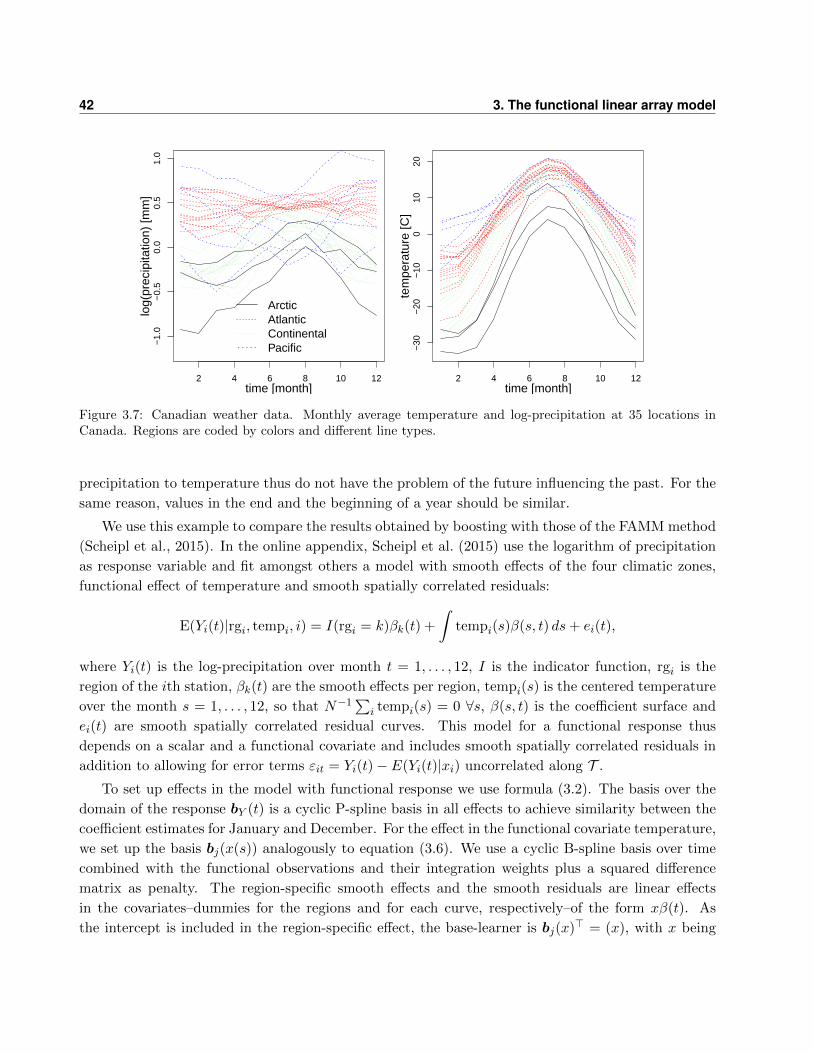
42 3. The functional linear array model
2 4 6 8 10 12
−1.
0−
0.5
0.0
0.5
1.0
ArcticAtlanticContinentalPacific
time [month]
log(
prec
ipita
tion)
[mm
]
2 4 6 8 10 12
−30
−20
−10
010
20
time [month]te
mpe
ratu
re [C
]Figure 3.7: Canadian weather data. Monthly average temperature and log-precipitation at 35 locations inCanada. Regions are coded by colors and different line types.
precipitation to temperature thus do not have the problem of the future influencing the past. For the
same reason, values in the end and the beginning of a year should be similar.
We use this example to compare the results obtained by boosting with those of the FAMM method
(Scheipl et al., 2015). In the online appendix, Scheipl et al. (2015) use the logarithm of precipitation
as response variable and fit amongst others a model with smooth effects of the four climatic zones,
functional effect of temperature and smooth spatially correlated residuals:
E(Yi(t)|rgi, tempi, i) = I(rgi = k)βk(t) +
∫tempi(s)β(s, t) ds+ ei(t),
where Yi(t) is the log-precipitation over month t = 1, . . . , 12, I is the indicator function, rgi is the
region of the ith station, βk(t) are the smooth effects per region, tempi(s) is the centered temperature
over the month s = 1, . . . , 12, so that N−1∑
i tempi(s) = 0 ∀s, β(s, t) is the coefficient surface and
ei(t) are smooth spatially correlated residual curves. This model for a functional response thus
depends on a scalar and a functional covariate and includes smooth spatially correlated residuals in
addition to allowing for error terms εit = Yi(t)− E(Yi(t)|xi) uncorrelated along T .
To set up effects in the model with functional response we use formula (3.2). The basis over the
domain of the response bY (t) is a cyclic P-spline basis in all effects to achieve similarity between the
coefficient estimates for January and December. For the effect in the functional covariate temperature,
we set up the basis bj(x(s)) analogously to equation (3.6). We use a cyclic B-spline basis over time
combined with the functional observations and their integration weights plus a squared difference
matrix as penalty. The region-specific smooth effects and the smooth residuals are linear effects
in the covariates–dummies for the regions and for each curve, respectively–of the form xβ(t). As
the intercept is included in the region-specific effect, the base-learner is bj(x)> = (x), with x being

3.7 Discussion 43
a dummy vector of length 4. For the smooth residuals ei(t), we enforce the default sum-to-zero-
constraint at each t, cf. Section 3.2. For the region specific effect, we use a Ridge-penalty by setting
the penalty to the four-dimensional identity matrix P j = I4. The spatial correlation of the residual
curves is accommodated by using the inverse of a spatial correlation matrix as penalty matrix P j .
Following Scheipl et al. (2015), we use a Matern correlation matrix with smoothness parameter 0.5
and range 310 kilometers, which implies a rather strong correlation.
The optimal stopping iteration for 25-fold bootstrapping over curves is so small that the base-
learner for smooth residual curves is not selected (mstop=30). If the optimal stopping iteration is
determined by leaving-one-curve-out cross-validation, it can be seen that for three weather stations
the out-of-bag prediction is quite bad and getting worse for higher mstop, causing the optimum of the
mean to be very small. Those three stations are Pr. Ruppert (14), Kamploos (15) and Resolute (34)
(numbers in brackets correspond to numbers in Figure 3.9). When looking at the median over the
squared errors the optimal stopping iteration is much higher (mstop=205) so that the base-learner
for the smooth residuals is selected into the model. As the effects for region and temperature are
very similar irrespective of the number of boosting iterations, we limit the representation of results
to the model with mstop=205, as it includes all effects. Figure 3.8 shows the estimated coefficients for
the regions and the effect of temperature on log-precipitation. In general the precipitation is lowest
in spring and highest in summer. An exception is the Pacific region where the highest precipitation
values are measured in winter. Stations in the Atlantic region have the highest precipitations during
the whole year. In the Continental region differences between the seasons are most pronounced. The
effect of temperature on log-precipitation changes over the year. Higher temperatures in spring and
summer are associated with lower precipitation over the whole year whereas higher temperatures in
autumn and winter are associated with higher precipitation values. The association of temperature
and precipitation is stronger in the winter than in the summer. Figure 3.9 shows the smooth residual
curves. They vary in the range of -0.4 to 0.4. The most extreme smooth residuals are estimated for the
Pacific region, where precipitation is relatively variable on a small spatial scale indicating additional
unmeasured covariates besides the regional and spatial effects. The uncorrelated error terms εit are
quiet small compared to the smooth residual curves ei(t). Comparing the results obtained by FAMM
(Scheipl et al., 2015) and boosting, the estimates for the effects of region and temperature are very
similar. The estimated spatially correlated smooth residuals are similar in part but different for some
stations.
3.7 Discussion
In this chapter, we introduced Functional Linear Array Models (FLAMs), a generic model class for
functional data measured on a common grid with potential missings. The response can be scalar or
functional. The FLAM has a modular structure: the transformation function allows to choose which
feature of the conditional distribution of the response to model and the additive predictor allows the
specification of a variety of covariate effects. We take advantage of the Kronecker product structure
of the design matrix to achieve computational efficiency using linear array models. The optimization
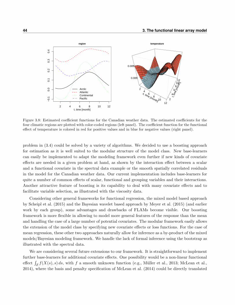
44 3. The functional linear array model
2 4 6 8 10 12
−0.
10.
00.
10.
20.
30.
4
region
t, time [month]
ArcticAtlanticContinentalPacific
s, time [month]
24
68
1012
t, tim
e [m
onth
]
2
4
681012
0.000
0.005
temperature
Figure 3.8: Estimated coefficient functions for the Canadian weather data. The estimated coefficients for thefour climatic regions are plotted with color-coded regions (left panel). The coefficient function for the functionaleffect of temperature is colored in red for positive values and in blue for negative values (right panel).
problem in (3.4) could be solved by a variety of algorithms. We decided to use a boosting approach
for estimation as it is well suited to the modular structure of the model class. New base-learners
can easily be implemented to adapt the modeling framework even further if new kinds of covariate
effects are needed in a given problem at hand, as shown by the interaction effect between a scalar
and a functional covariate in the spectral data example or the smooth spatially correlated residuals
in the model for the Canadian weather data. Our current implementation includes base-learners for
quite a number of common effects of scalar, functional and grouping variables and their interactions.
Another attractive feature of boosting is its capability to deal with many covariate effects and to
facilitate variable selection, as illustrated with the viscosity data.
Considering other general frameworks for functional regression, the mixed model based approach
by Scheipl et al. (2015) and the Bayesian wavelet based approach by Meyer et al. (2015) (and earlier
work by each group), some advantages and drawbacks of FLAMs become visible. Our boosting
framework is more flexible in allowing to model more general features of the response than the mean
and handling the case of a large number of potential covariates. The modular framework easily allows
the extension of the model class by specifying new covariate effects or loss functions. For the case of
mean regression, these other two approaches naturally allow for inference as a by-product of the mixed
models/Bayesian modeling framework. We handle the lack of formal inference using the bootstrap as
illustrated with the spectral data.
We are considering several future extensions to our framework. It is straightforward to implement
further base-learners for additional covariate effects. One possibility would be a non-linear functional
effect∫S f(X(s), s) ds, with f a smooth unknown function (e.g., Muller et al., 2013; McLean et al.,
2014), where the basis and penalty specification of McLean et al. (2014) could be directly translated

3.7 Discussion 45
2 4 6 8 10
−0.
40.
00.
4Dawson (1)
● ●
●
●
● ●● ● ●
●● ●
2 4 6 8 10
−0.
40.
00.
4
Whitehorse (2)
●● ●
●●
● ● ●●
● ● ●
2 4 6 8 10
−0.
40.
00.
4
Yellowknife (3)
● ●●
●● ● ●
●●
● ●
●
2 4 6 8 10
−0.
40.
00.
4
Uranium City (4)
●●
●●
●● ● ●
●● ●
●
2 4 6 8 10
−0.
40.
00.
4
Churchill (5)
●●
● ● ● ● ●●
● ●●
●
2 4 6 8 10
−0.
40.
00.
4
Edmonton (6)
●
●●
●●
● ●● ●
●●
●
2 4 6 8 10
−0.
40.
00.
4
Pr. Albert (7)
● ● ● ●●
● ●● ●
● ●●
2 4 6 8 10
−0.
40.
00.
4The Pas (8)
● ●● ●
●
● ● ●●
● ● ●
2 4 6 8 10
−0.
40.
00.
4
Calgary (9)
● ●●
●
●●
●●
●
● ● ●
2 4 6 8 10
−0.
40.
00.
4
Regina (10)
● ● ●●
● ●●
●●
●
●
●
2 4 6 8 10
−0.
40.
00.
4
Winnipeg (11)
●●
●● ● ●
●● ●
● ● ●
2 4 6 8 10
−0.
40.
00.
4
Thunder Bay (12)
●●
● ● ● ●● ●
●● ●
●
2 4 6 8 10
−0.
40.
00.
4
Pr. George (13)
●● ● ●
●
●● ● ● ●
● ●
2 4 6 8 10
−0.
40.
00.
4
Pr. Rupert (14)
● ●●
●● ● ●
●●
●
● ●
2 4 6 8 10
−0.
40.
00.
4Kamloops (15)
●
●
●
●
●
● ● ●●
●
●●
2 4 6 8 10
−0.
40.
00.
4
Vancouver (16)
● ● ● ● ● ●● ●
●● ●
●
2 4 6 8 10
−0.
40.
00.
4
Victoria (17)
● ●●
● ●●
●● ●
●●
●
2 4 6 8 10
−0.
40.
00.
4
Scheffervll (18)
●
● ●●
●● ●
●● ●
●●
2 4 6 8 10
−0.
40.
00.
4
Bagottville (19)
● ● ● ●● ●
●● ●
● ● ●
2 4 6 8 10
−0.
40.
00.
4
Arvida (20)
● ● ●●
● ●●
●●
●●
●
2 4 6 8 10
−0.
40.
00.
4
St. Johns (21)
● ● ● ● ● ●●
● ● ●● ●
2 4 6 8 10
−0.
40.
00.
4Quebec (22)
● ● ●●
● ● ● ● ●●
● ●
2 4 6 8 10
−0.
40.
00.
4
Fredericton (23)
● ● ● ●● ● ●
● ● ● ● ●
2 4 6 8 10
−0.
40.
00.
4
Sydney (24)
● ● ● ●● ● ● ● ●
● ● ●
2 4 6 8 10
−0.
40.
00.
4
Ottawa (25)
●● ● ● ● ● ● ● ●
●● ●
2 4 6 8 10
−0.
40.
00.
4
Montreal (26)
● ● ● ●●
● ●● ●
●●
●
2 4 6 8 10
−0.
40.
00.
4
Sherbrooke (27)
● ●● ● ● ● ● ●
●●
● ●
2 4 6 8 10
−0.
40.
00.
4
Halifax (28)
● ● ● ● ● ● ● ●●
● ● ●
2 4 6 8 10
−0.
40.
00.
4Yarmouth (29)
● ● ● ● ● ● ● ● ● ● ● ●
2 4 6 8 10
−0.
40.
00.
4
Toronto (30)
● ●●
●● ●
● ●●
●●
●
2 4 6 8 10
−0.
40.
00.
4
London (31)
● ●● ●
●● ● ● ●
●● ●
2 4 6 8 10
−0.
40.
00.
4
Charlottvl (32)
● ● ● ● ● ●● ● ● ● ● ●
2 4 6 8 10
−0.
40.
00.
4
Inuvik (33)
●●
● ●●
● ●●
●
●●
●
2 4 6 8 10
−0.
40.
00.
4
Resolute (34)
●●
●●
●●
●●
●●
● ●
2 4 6 8 10
−0.
40.
00.
4
Iqaluit (35)
● ● ●●
● ●● ● ●
● ●●
●
0
0
1
23
4 5
6 7 89 10 11
12
1314
151617
18
1920 2122 23 2425 26 27 2829303132
33
34
35
Figure 3.9: Estimated residuals for the Canadian weather data. The estimated smooth spatially correlatedresidual curves ei(t) (lines) and the uncorrelated error terms εit (circles) are plotted with regions color-coded.The locations of the weather stations are given in the map at the bottom.

46 3. The functional linear array model
to a new base-learner. Another is to use a different set of basis functions in the estimation of linear
functional effects. For instance, one could use the eigenfunctions of the estimated covariance function
as basis functions for bY (t), as is commonly done in the context of functional principal component
analysis (e.g., Scheipl et al., 2015).
Another interesting direction is to use boosting for functional regression models that cannot be
written as linear array models. This would allow for responses observed on irregular grids and for
functional effects whose integration limits depend on the current observation point of the response.
For instance, if functional response and covariate are observed over time, the historical functional
linear model (Malfait and Ramsay, 2003; Harezlak et al., 2007) ξ(Y (t)|X = x) =∫ tt−δ x(s)β(s, t) ds,
can be of interest, where only lagged past values of the functional covariate are used to model the
current value of the response. This extension to non-array models that allows for functional historical
effects is discussed in the next chapter.
Acknowledgments
We acknowledge support from the German Research Foundation through Emmy Noether grant GR
3793/1-1 (Sarah Brockhaus, Fabian Scheipl and Sonja Greven). Special thanks to Benjamin Hofner
for his advice on stability selection. Thanks to Wolfgang Raffelt for providing us with the viscosity
data and to the Siemens AG for the spectral data of fossil fuels. We thank the referees and the editor
for their useful comments.
Chapter 4
Functional regression models with
many historical effects
Contributing manuscript
This chapter is based on the following paper:
Brockhaus, S., Melcher, M., Leisch, F., and Greven, S. (2016): Boosting flexible func-
tional regression models with a high number of functional historical effects. Statistics and
Computing, accepted, DOI: http://dx.doi.org/10.1007/s11222-016-9662-1.
This is joint work with Michael Melcher (Institute of Applied Statistics and Computing, University of
Natural Resources and Life Sciences, Vienna, Austria), Friedrich Leisch (Institute of Applied Statistics
and Computing, University of Natural Resources and Life Sciences, Vienna, Austria) and Sonja
Greven (Department of Statistics, LMU Munich, Germany). The idea to analyze a biotechnological
dataset on fermentation processes using FDA techniques originated in a cooperation between Sonja
Greven and Friedrich Leisch. Michael Melcher gave background information on the data and wrote
the description of the dataset at the beginning of Section 4.6. The methodological developments
were mainly conducted by Sarah Brockhaus and Sonja Greven. In particular, Sonja Greven gave
considerable input on identifiability. Sarah Brockhaus extended the existing software in the R package
FDboost (Brockhaus and Rugamer, 2016) to historical models, conducted the simulation study and
the data analysis and wrote the manuscript under the supervision of the other three authors. All
authors were involved in proofreading the manuscript. Except for minor changes, Chapter 4 and
Brockhaus et al. (2016b) are identical.
Parts of Chapter 4 are contained in the conference proceedings of IWSM 2015 (30th International
Workshop on Statistical Modelling), see Greven (2015).
Software
The analyses presented in this chapter were conducted using R version 3.1.2 (R Core Team, 2015).
For boosting functional regression models, FDboost 0.0-8 (Brockhaus and Rugamer, 2016) along with

48 4. Functional regression models with many historical effects
mboost 2.4-2 (Hothorn et al., 2016) were used. Functional regression models based on mixed models
were fitted by the R add-on package refund 0.1-12 (Huang et al., 2016). For data preprocessing, the
package robfilter 4.0 was used (Fried et al., 2012); see Appendix C.3.
4.1 Introduction
Functional data consist of a sample of functions observed on a finite grid in some continuous domain
(Ramsay and Silverman, 2005). The analysis of functional data, for instance, by regression models,
has become more and more important as technical advances increasingly generate such data (e.g.,
Morris, 2015). We develop a general framework for functional regression models where the functional
responses can be observed on curve-specific grids and the covariates can vary over the domain of the
response. This includes the case where functional response and functional covariates are observed
over the same time interval. In this case the response at a given time-point is usually thought to be
influenced only by covariate observations up to this current time-point. This model is called historical
functional model as only the history (and not the future) of the covariate influences the current value of
the response; see Malfait and Ramsay (2003), Harezlak et al. (2007) and Gervini (2015) for historical
functional models with a single functional covariate. It is also possible to restrict the functional
historical effect to a certain lag in the past (e.g., Kim et al., 2011). For the limiting case of lag zero,
a concurrent effect is obtained, where the response is only influenced by the concurrent value of the
covariate (Ramsay and Silverman, 2005). The concurrent model can be seen as a varying-coefficient
model (Hastie and Tibshirani, 1993), where the effect varies over time.
The motivation for the development of flexible regression models including many historical and
concurrent functional effects comes from a biotechnological dataset consisting of 25 Escherichia coli
bacterial fermentations for the production of a model protein (Melcher et al., 2015). A major draw-
back of such bioprocesses is the inaccessibility of key process parameters such as the cell dry mass
(CDM), which have to be determined offline in cost- and labor-intensive measurements. On the other
hand, various physical process variables (e.g., pressure, base- or O2-consumption) can be measured
easily without significant costs and additional chemical information is obtained online via fluorescence
spectroscopy and mass spectrometry. Based on these sensor signals a prediction of the CDM would
be desirable to allow for an online monitoring of the process (Striedner and Bayer, 2013). As during
a fermentation only observations up to the current time-point can be used, historical and concurrent
models using the online measured variables as covariates to predict the CDM are of interest. The po-
tentially large number of variables (p > n setting) is a great challenge and makes it impossible to use
existing methods for historical models. Additionally, this makes variable selection highly important,
which is widely unaddressed in regression with functional response.
In our approach, estimation is conducted by a component-wise gradient boosting algorithm (e.g.,
Buhlmann and Hothorn, 2007), which allows to fit models with many effects, including more pa-
rameters than observations, and automatically does model selection. Versatile effects of scalar and
functional covariates can be specified, in particular functional effects with integration limits depending
on the current time of the response. Boosting can fit models for different features of the conditional
4.2 The functional regression model with many historical effects 49
response distribution by optimizing the corresponding loss functions, yielding, e.g., quantile regression
or (generalized) mean regression models.
In Chapter 3, we introduced a general framework for functional regression, which could deal with
a high number of covariates and variable selection by using boosting for estimation. However, the
estimation framework is based on the array models by Currie et al. (2006), and thus the covariates
need to be constant over the domain of the response and the functional responses have to be observed
on equal grids. Both of these requirements are not fulfilled for the functional historical model applied
to a functional response with curve-specific grids, such as in our application. To overcome these
restrictions and motivated by models with functional historical effects, we introduce in this chapter
a general framework for functional response regression without relying on arrays. In addition to
functional historical effects, this allows the inclusion of, e.g., (smooth) effects of scalar covariates,
linear effects of functional covariates and different interaction terms.
The only existing model class allowing for a functional response with curve-specific grids and such
a variety of covariate effects, including functional historical effects, was introduced by Ivanescu et al.
(2015) and Scheipl et al. (2015) as functional additive mixed models (FAMMs). Using a mixed models
representation, mean regression models with a moderate number of effects are feasible. The models
are restricted to the conditional mean of the response and require more observations than coefficients
to be estimable. In practice, the number of covariate effects is noticeably limited by memory and
computation time. In particular, the high number of functional covariates in our application (more
than observations) could not be handled by the FAMM framework.
This chapter is organized as follows: First, the functional regression model with many historical
effects is presented (Section 4.2). We introduce two new parameterizations of the functional historical
effect and discuss identifiability. In Section 4.3, we discuss several extensions, leading to a more
general framework for additive functional models that allows for a large number of different and
flexible covariate effects and thus is considerably extending the model in Section 4.2. The estimation
of the models by a component-wise gradient boosting algorithm is explained in Section 4.4. For an
empirical evaluation of our methods, we conduct a simulation study (Section 4.5). We use historical
and concurrent models to analyze the fermentation dataset (Section 4.6). The chapter concludes with
a discussion in Section 4.7. Additional information on identifiability checks for functional historical
effects are given in Appendix A.2. More details on the simulation and the application can be found
in Appendix C.
4.2 The functional regression model with many historical effects
We assume that we observe realizations from (Y,X) taking values in Y ×X , where Y given X follows
a conditional distribution FY |X and X can be random or fixed. Let Y be a suitable space for the
functional responses such as the space of square integrable functions L2(T , µ), with T being a real-
valued interval and µ the Lebesgue measure. We set T = [T1, T2], with T1, T2 ∈ R and T1 < T2. Let Xbe the product space of J L2(S, µ) spaces, with S = T , as response and covariates have to be measured
on a common domain for historical effects to be meaningful. In practice, we observe data (yi, xi),
50 4. Functional regression models with many historical effects
i = 1 . . . , N , that are assumed to come from the above model. Each of the N response trajectories
is observed at curve-specific points (ti1, . . . , tiGi)>, tig ∈ T , resulting in n =
∑iGi observed points
in total. If the functional response is observed on one common grid, we denote it by (t1, . . . , tG)>.
For each functional covariate xj(s), we assume that it is observed on a common grid (s1, . . . , sR)>,
sr ∈ S. The grid points can vary between the different functional covariates, but we omit this possible
dependency on j for better readability. Generally, we use upper case for random variables and lower
case for realizations. For the covariates, indexing over i refers to the observed case i and indexing
over j to one of the J covariates. Consider the functional model for the expectation of the response
with J historical effects
E(Y (t)|X = x) =J∑j=1
∫ t
T1
xj(s)βj(s, t) ds, (4.1)
where βj(s, t) is the coefficient surface of the covariate xj with triangular support. For J = 1, such
models were considered by Malfait and Ramsay (2003), Harezlak et al. (2007) and Gervini (2015).
The integration limits can be generalized to∫ u(t)
l(t)xj(s)βj(s, t) ds, (4.2)
where l(t) and u(t) depend on the current time-point t of the response and l(t) ≤ u(t) for all t ∈ T . A
common specification for a more general historical effect is l(t) = max(T1, t− δ) for a fixed lag δ > 0
and u(t) = t (Malfait and Ramsay, 2003; Harezlak et al., 2007). For δ ≥ |T |, with |T | = T2 − T1,
the special case of (4.1) is obtained, with integration limits {T1, t}, indicating that the whole past of
the covariate can influence the response, and with the coefficient function β(s, t) being non-zero on
the triangle with s ≤ t. For δ < |T |, only values of xj(s) within the lag δ can influence the response
and the coefficient function βj(s, t) is defined on a trapezoidal area with max(T1, t − δ) ≤ s ≤ t. In
the special case of fixed integration limits l(u) = T1 and u(t) = T2, one obtains the standard linear
function-on-function effect, which we will call unconstrained functional effect in the following (e.g.,
Morris, 2015). In our framework it is possible to consider hybrid models combining possibly many
historical, concurrent and unconstrained functional effects with effects of scalar variables, see also
Section 4.3. The only framework allowing for general integration limits as in (4.2) and hybrid models
is the FAMM framework by Scheipl et al. (2015), which is limited to a moderate number of covariate
effects.
Following Scheipl et al. (2015), the integral in the historical effect can be approximated by a
numerical integration scheme as∑R
r=1 xj(sr, t)βj(sr, t). Here, the transformed observations xj(sr, t)
are defined as
xj(sr, t) = I [l(t) ≤ sr ≤ u(t)] ∆(sr)xj(sr),
with integration weights ∆(s) and indicator function I. The coefficient function βj(s, t) is represented
using spline basis functions Φk(s), k = 1, . . . ,Kj , in s- and Φl(t), l = 1, . . . ,KY , in t-direction.
4.2 The functional regression model with many historical effects 51
Assuming that the coefficient function βj(s, t) lies in the span of the basis functions Φk(s)Φl(t), we
represent the historical effect (4.2) as:
∫ l(t)
u(t)xj(s)βj(s, t) ds =
∫ l(t)
u(t)xj(s)
Kj∑k=1
KY∑l=1
Φk(s)Φl(t)θj,kl ds
≈R∑r=1
xj(sr, t)
Kj∑k=1
KY∑l=1
Φk(sr)Φl(t)θj,kl,
(4.3)
with coefficient vector θj = (θj,11, . . . , θj,KjKY)>. We regularize effect (4.3) using a quadratic penalty
term, θ>j P jY θj , with penalty matrix (Wood, 2006, Sec. 4.1.8)
P jY = λj(P j ⊗ IKY) + λY (IKj ⊗ P Y ), (4.4)
where P j ∈ RKj×Kj and P Y ∈ RKY ×KY are appropriate penalty matrices for the bases Φk(s) and
Φl(t), and λj , λY ≥ 0 are smoothing parameters.
4.2.1 Alternative parameterizations of the functional historical effect
In the functional historical effect, the length of the integration interval is changing with t. The
idea of considering reparameterizations is to compensate for the differing length of the integration
interval. Although equivalent in theory, the different parameterizations yield different model fits in
practice because of the smoothing penalties. Following ideas that Gellar et al. (2014) developed for
scalar-on-function regression with functional covariates having variable domains, we introduce two
variants of reparameterizations for the functional historical effect in (4.2). The first quite intuitive
parameterization is to divide the historical effect by the length of the integration interval:
1
u(t)− l(t)
∫ u(t)
l(t)xj(s)βj(s, t) ds. (4.5)
For the limiting case u(t)−l(t) ↓ 0, we use the fundamental theorem of calculus, limt↓0(1/t)∫ t
0f(s) ds =
f(0), and thus set (4.5) to xj(u(t))βj(u(t), t) for u(t) − l(t) ↓ 0. With this standardization, a con-
stant coefficient function results in a constant effect if the functional variable is constant. The
standardized coefficient function βj(s, t) can be converted into the historical effect using βj(s, t) ≈{u(t)− l(t)}βj(s, t) for u(t) > l(t).
The second approach is to standardize the time interval [l(t), u(t)] to [0, 1] by computing a new
time variable v = s−l(t)u(t)−l(t) for each t, inducing the transformed functional variable x(v) and coefficient
function β(v, t) ≈ [u(t)− l(t)]β(s, t). Consequently, the reparameterized effect can be written as∫ 1
0xj(v)βj(v, t) dv. (4.6)

52 4. Functional regression models with many historical effects
The limiting case u(t)− l(t) ↓ 0 is treated analogously to above. Because of the common domain [0, 1]
of the transformed covariate xj(v), the domain of the coefficient function βj(v, t) is rectangular. For
the special case of [l(t), u(t)] = [0, t], this parameterization yields v = s/t and thus the coefficient is
βj(s/t, t) ≈ t β(s, t).
4.2.2 Identifiability of the functional historical effect
Identifiability is a model property meaning that no two distinct parameter values θ give the same
distribution of Y , where Y comes from a given model depending on θ. Here, θ corresponds to θjunder the assumption that βj(s, t) lies in the span of basis functions Φk(s)Φl(t), cf. equation (4.3).
Considering for each t the restriction of the functional variable Xj(s) to the integration interval
[l(t), u(t)], {Xj(s)|s ∈ [l(t), u(t)]}, we denote the covariance operator of that restricted functional
variable by KXj (t). In theory, the coefficient function βj(s, t) of a historical effect is identifiable up
to the addition of functions β∗j (s, t) that lie in the null space of KXj (t) for each t. That means for
such β∗j (s, t) that ∫ u(t)
l(t)Xj(s)βj(s, t) ds =
∫ u(t)
l(t)Xj(s){βj(s, t) + β∗j (s, t)} ds
for all t. Thus, βj(s, t) is identifiable if the null space of KXj (t) is trivial for all t. This is well known
for the unconstrained functional effect with fixed integration limits, see, e.g., Scheipl and Greven
(2016).
In the present regression context, it is practically more relevant to ask whether for a given set of
observed covariates two distinct parameters θ can give the same conditional distribution for the
vector of responses. Moreover, as we have finite sample finite grid data, it is important to ask
whether for a given set of observed covariates on their given grid, two distinct parameters θ can give
the same conditional distribution for the vector of responses on their given grids. For a given set of
covariate observations xj(s), the coefficient vector θj in (4.3) that defines βj(s, t) is identifiable if the
design matrix for effect j has full rank. For functional historical effects, this requirement reduces to
having a full rank design matrix in the functional covariate, defined in (4.10), for all t. Numeric rank
deficiency of a matrix can be detected by its condition number κ, which is computed as the ratio
between its highest and lowest eigenvalue. A high condition number (we use κ > 106) is evidence for
numeric rank deficiency. We compute the condition number for submatrices of the marginal design
matrix for each t; see Appendix A.2.1 for details on the design matrices and Appendix A.2.2 for the
computation of the condition numbers.
In the case of a rank deficient design matrix we can still get a unique coefficient under the additional
assumption that the coefficient function is smooth in a certain sense. The idea is that a parameter
vector θj which results in the smoothest surface βj(s, t) is chosen as the most plausible representative
from among all the parameter vectors yielding identical linear predictor values. This assumption is
encoded in a suitable smoothness penalty, similar to a Bayesian prior. Uniqueness of the representative
and consequently of the estimate is ensured for the unconstrained functional effect if the penalty
matrix in s direction P j , defined as in (4.4), and the functional covariate do not have a null space
4.3 Extension to the general model 53
overlap (Scheipl and Greven, 2016), which is defined as the amount of overlap between the span
of the two null spaces. To measure null space overlap more adequately for a historical effect, we
introduce a new measure for the maximal null space overlap between successive submatrices of the
functional covariate and the penalty matrix; see Appendix A.2.3 for details. Null space overlap
between functional observations and penalty can be avoided by using a penalty matrix with full rank.
In order to maintain the smoothing properties of the penalty, Scheipl and Greven (2016) propose
as one option to use a penalty adding a small amount of shrinkage for vectors not penalized by the
original penalty (Marra and Wood, 2011) resulting in a full rank penalty.
4.3 Extension to the general model
We now discuss several extensions of model (4.1) to (4.3) allowing for (a) more general features of the
conditional response distribution to be modeled than the mean and for (b) a range of flexible effects
of scalar and functional covariates in addition to the historical effects so far considered. We again
assume that we observe realizations from (Y,X) taking values in Y × X as for model (4.1), with the
generalization that the covariates can be scalar or functional with differing domains, and thus X is
a product space of the real numbers R for scalar covariates and L2(Sj , µ) for functional covariates,
with real intervals Sj . Similarly to model (3.1) in Chapter 3, the following additive regression model
serves as generic model:
ξ(Y |X = x) = h(x) =J∑j=1
hj(x), (4.7)
where ξ is a transformation function choosing the feature of the conditional distribution to be modeled,
such as the expectation or some quantile. A generalized linear model (Nelder and Wedderburn, 1972)
can be represented using the composition of expectation and link function as the transformation
function. The linear predictor h(x) is the sum of partial effects hj(x). Each partial effect hj(x) is
a real-valued function over T and typically depends on one covariate xj in x, but more generally it
can depend on a subset of covariates to form interaction effects. In Table 2.1, an overview of possible
partial effects is given, including, e.g., linear or smooth effects of scalar covariates, group-specific
effects, and interactions between scalar and functional covariates. In contrast to representation (3.2)
in Chapter 3, each effect hj(x) is defined using the general basis representation
hj(x)(t) = bjY (x, t)>θj , j = 1, . . . , J, (4.8)
where bjY (x, t) is a vector of basis evaluations and θj is the corresponding vector of coefficients.
Depending on the effects hj , additional constraints on the effects are necessary to obtain an identifiable
model; see Appendix A for a discussion. As in Scheipl et al. (2015), the effects are represented using
54 4. Functional regression models with many historical effects
the row tensor product � of two marginal bases bj : X × T → RKj and bY : T → RKY with a
coefficient vector θj ∈ RKjKY :
hj(x)(t) =(bj(x, t)
> � bY (t)>)θj . (4.9)
The row tensor product � of two marginal design matrices, Bj ∈ Rn×Kj with rows bj(xij , tig)> and
BY ∈ Rn×KY with rows bY (tig)>, is defined as n×KjKY matrix Bj�BY = (Bj⊗1>KY
) ·(1>Kj⊗BY ),
where ⊗ is the Kronecker product, · denotes entry-wise multiplication, also called Hadamard product,
and 1K denotes the K-dimensional vector of ones. Regularization is achieved by a Ridge-type penalty
and the quadratic penalty term is constructed as in equation (4.4), with marginal penalty matrices
P j and P Y suitable for bj(x, t) and bY (t) respectively.
Representation (4.9) is a special case of (4.8) but more general than the functional linear array
model (FLAM), introduced in Chapter 3. The FLAM corresponds to the special case where the
design matrix has the form of a Kronecker product Bj �BY = (Dj ⊗1G)� (1N ⊗DY ) = Dj ⊗DY .
The Kronecker product in particular requires that the basis can be split into two marginal parts with
the part DY independent of i for all response curves, which is fulfilled if the response curves are
observed on one common grid (t1, . . . , tG)>, and the part Dj for the covariate independent of t. The
latter requirement is not fulfilled for historical effects, where integration limits depend on t and the
covariate basis bj(x, t) thus changes with t.
Compared to FAMMs (Scheipl et al., 2015), where historical effects and responses observed on
unequal grids are possible but only the conditional expectation can be modeled, our framework allows
for more general transformation functions ξ. The number of effects that can be estimated is limited
in FAMMs due to the likelihood-based estimation and would not accommodate p > n settings as in
our application, whereas our framework gives the possibility to specify models with a large number
of effects.
The functional historical model (4.1) to (4.3) is a special case of the more general framework (4.7)
by letting ξ = E and taking the marginal basis over the functional covariate xj(s) to be
bj(x, t)> ≈ [xj(s1, t) · · · xj(sR, t)] [Φj(s1) · · · Φj(sR)]>
=
[R∑r=1
xj(sr, t)Φ1(sr) · · ·R∑r=1
xj(sr, t)ΦKj (sr)
],
(4.10)
where Φj(s)> = [Φ1(s) · · · ΦKj (s)] and xj(sr, t) as defined in (4.3). The basis over the index of the
response t is bY (t)> = ΦY (t)> = [Φ1(t) · · · ΦKY(t)].
Embedding the functional historical model into the general framework (4.7) allows several flexible
extensions of model (4.1) to (4.3) depending on the requirements of the given application. Possibil-
ities include the combination of different historical, concurrent and unconstrained effects of several
functional covariates, interactions with or linear/smooth effects of scalar covariates, and/or different
features of the conditional response distribution to be modeled such as median regression for more
robustness in the presence of outlying values.
4.4 Estimation by gradient boosting 55
4.4 Estimation by gradient boosting
We use a component-wise gradient boosting algorithm to estimate the functional regression model
in (4.7); see, e.g., Buhlmann and Hothorn (2007) for an introduction to boosting from a statistical
point of view. The idea of boosting is to enhance the performance of simple models, the so-called
base-learners, by combining them. Gradient boosting is a gradient descent algorithm minimizing the
empirical risk with respect to the linear predictor h. In component-wise boosting, in each step only
the best fitting base-learner as an approximation to the negative gradient is selected for the model
update. As only one base-learner is used at a time, a large number of base-learners can be considered.
Usually, the boosting algorithm is stopped before convergence, so-called early stopping, to obtain
regularized effect estimates. In our setting, the base-learners are the penalized models for the effects
hj as defined in equation (4.9) with penalty (4.4). For a model containing J historical effects, each of
the j = 1, . . . , J base-learners represents one historical effect and thus corresponds to one candidate
covariate.
We define a suitable loss for functional responses in the following. Let ρ : (Y × X ) × H →L1(T , µ), where H is the set of all functions from (X × T ) to L2(T , µ), be a loss function, which is
differentiable with respect to the second argument. The loss ρ could, e.g., be the squared error loss
ρL2 ((Y,X), h) (t) = 12(Y −h(X))2(t), which yields the expectation as population minimizer. The loss
of a whole trajectory ` : (Y × X )×H → [0,∞) is defined as
` ((Y,X), h) =
∫Tρ ((Y,X), h) (t) dt.
Boosting aims at minimizing the expected loss, the so-called risk
h∗ = arg minh
E ` ((Y,X), h) .
In practice, the expectation is approximated by the mean over observed data (yi, xi), i = 1, . . . , N ,
and the integral by a numerical integration scheme. Thus, boosting optimizes the empirical risk
h∗ = arg minh
N∑i=1
Gi∑g=1
wi∆(tig)ρ ((yi, xi), h) (tig),
where wi are sampling weights for whole trajectories and ∆(t) are weights of a numerical integration
scheme. The weights wi can be used to weight the observations in the model fit or in resampling
methods.
The boosting algorithm is similar to the one used in Chapter 3. The essential difference is the
abandonment of the array structure, which allows for response trajectories observed on unequal grids
and covariates that vary over the domain of the response. Both features are necessary for the data
and model (4.1) considered in our application. In detail, the used boosting algorithm is as follows.

56 4. Functional regression models with many historical effects
Algorithm: Gradient boosting for functional regression models
Step 1: Define the bases bjY (x, t) and penalties P jY for the j = 1, . . . , J base-learners. Define
the weights wig = wi∆(tig), for the observations i = 1, . . . , N , g = 1, . . . , Gi. Initialize the
parameters θ[0]j . Select the step-length ν ∈ (0, 1) and the stopping iteration mstop. Set m := 0.
Step 2: Compute the negative gradient of the empirical risk
ui(tig) := − ∂
∂hρ ((yi, xi), h) (tig)
∣∣∣∣h=h[m]
,
with h[m](xi)(tig) =∑J
j=1 bjY (xi, tig)>θ
[m]j .
Fit the base-learners for j = 1, . . . , J :
γj = arg minγ∈RKjKY
N∑i=1
Gi∑g=1
wig
{ui(tig)− bjY (xi, tig)
>γ}2
+ γ>P jY γ,
with weights wig and penalty matrices P jY .
Select the best fitting base-learner according to a least squares criterion:
j? = arg minj=1,...,J
N∑i=1
Gi∑g=1
wig
{ui(tig)− bjY (xi, tig)
>γj
}2
Step 3: Update the parameters θ[m+1]j? = θ
[m]j? + νγj? and keep all other parameters fixed, i.e.,
θ[m+1]j = θ
[m]j , for j 6= j?.
Step 4: Unless m = mstop, increase m by one and go back to step 2.
The final model is ξ(Yi|Xi = xi) =∑
j h[mstop]j (xi). As offset in iteration 0 a smoothed mean or
median function is used for the smooth intercept. The other parameters θ[0]j are set to zero. In order
to get a fair selection of base-learners, it is important that all base-learners have the same degrees
of freedom (Hofner et al., 2011). This is achieved by choosing adequate smoothing parameters for
the penalty matrices P jY . In practice, we use the row tensor product representation (4.9) with
only one smoothing parameter per effect for both directions, simplifying the penalty in (4.4) to
P jY = λj(P j ⊗ IKY+ IKj ⊗ P Y ). Following Hofner et al. (2011), the degrees of freedom are
computed as df := trace(2Sj − S>j Sj), with hat matrix Sj = BjY
(B>jYBjY + P jY
)−1B>jY and
design matrix BjY = Bj � BY , as this definition is suitable when comparing two smooth terms
regarding the residual sum of squares (Buja et al., 1989). For fixed smoothing parameters λj and
fixed small step-length ν (usually ν = 0.1), the smoothness or complexity of the model terms is
controlled by the number of boosting iterations mstop (Friedman, 2001). Typically, the degrees of
freedom are chosen rather small. The smooth terms adapt to the complexity of the data by the
4.5 Simulation study 57
number of boosting iterations (Buhlmann and Yu, 2003). The optimal mstop is chosen by resampling
methods like cross-validation or bootstrap (see, e.g., Buhlmann and Hothorn, 2007). This can be
included in the algorithm by using the weights wi, which induces sampling on the level of curves.
To refine the model selection we use stability selection (Meinshausen and Buhlmann, 2010), which
is a method for selecting influential effects. Random samples of size bN/2c are drawn from the data
and in each subsample the model is fitted. We use complementary pairs stability selection (Shah
and Samworth, 2013), which improves the original procedure by resampling in complementary pairs
of mutually exclusive subsets of observations. Over the samples the relative frequency πj of being
selected among the first q base-learners is computed for each base-learner j = 1, . . . , J . The relative
frequencies πj are compared to a threshold πthr and all effects that are selected more frequently than
πthr are kept in the model. The parameters q and πthr are chosen such that an upper bound for the
per-family-error-rate (PFER) is kept, assuming that the selection procedure is not worse than random
guessing and that an exchangeability condition for the selection of noise variables holds. Intuitively,
the second assumption means that all noise variables are equally likely to be selected, see Meinshausen
and Buhlmann (2010) for details. Without those two assumptions Shah and Samworth (2013) derived
that the error bound holds for the expected number of “low selection probability variables”, when
the low selection probability corresponds to q/J , which is the average proportion of selected variables
per subsampling fold. For details on stability selection in the context of component-wise gradient
boosting, see Hofner et al. (2015a).
The boosting algorithm for functional regression models is implemented in the R add-on package
FDboost, which is based on the mboost package.
4.5 Simulation study
The simulation study is focused on the identifiability of the functional historical effects. We simulate
difficult settings, partially with rank deficient design matrix, to test the limits of the considered
models in very challenging settings. The motivation is that some of the bioprocess covariates in our
application exhibit low-rank behavior such as near linear increases. In order to have a competing
algorithm, we simulate a mean regression model with two functional historical effects. In this special
case–the transformation function ξ is the expectation and the model contains only a moderate
number of parameters–FAMMs (Scheipl et al., 2015) can be used to estimate model (4.7) using the
R package refund.
Basic model. As basic model we consider a functional historical model with two effects,
Yi(t) = β0(t) +2∑j=1
∫ t
T1
xij(s)βj(s, t) ds+ εit,
with s, t ∈ [1, 16], normally distributed errors, εit ∼ N(0, σ2ε), with the variance σ2
ε depending on the
signal-to-noise ratio. The signal-to-noise ratio is the ratio between the standard deviations of the

58 4. Functional regression models with many historical effects
linear predictor and the errors and is fixed at two. We generate data with N = 30 observation units,
22 irregularly spaced observations per response trajectory, and 100 observation points per functional
covariate. To vary the data generating mechanism, we use all combinations of the following settings:
1. Data generating processes for the functional covariates (see Figure C.1 in Appendix C.1 for
examples):
Covariates that are simulated using k ∈ {5, 10} cubic B-splines on equidistant knots as ba-
sis functions. The splines are weighted with random coefficients from a uniform distribution
U [−3, 3].
bsplines-k use k splines
local-k use k splines that are sampled out of 5k splines, resulting in trajectories with local
information
end-k use k splines that are sampled out of the last 3k splines using a total of 10k splines,
resulting in trajectories that have information in the end but are constant equal to zero at
the beginning
Covariates that are straight lines.
lines-0 parallel lines with random intercept ∼ N(−2, 1) and fixed slope 0.3
lines-1 lines with intercept 0 and random slope ∼ N(0, 0.1)
lines-2 lines with independent random intercept ∼ N(−2, 1) and random slope ∼ N(0, 0.1)
Note that some of these scenarios are meant to be very challenging as the end settings contain
no information at the beginning of the time interval from which to estimate the βj surface there,
and the lines settings contain at most two-dimensional information from which to estimate these
at least theoretically infinite-dimensional surfaces.
2. Number of nuisance variables that have no influence on the response, nuisance ∈ {0, 8}.
3. Random coefficient functions βj(s, t) are drawn using a tensor product of five marginal cubic
P-splines (Eilers and Marx, 1996) with random coefficients penalized by a first or second order
difference penalty matrix, dβ ∈ {1, 2}; see Appendix C.1 for details. The functional intercept
β0(t) is 1 + 2√t.
For each combination of the data generating process, we run 20 replications.
Estimation. For fitting, we use Kj = KY = 9 cubic B-splines on equally spaced knots and
vary the following settings:
1. Estimation algorithm: FAMM or boosting (FDboost).
2. Order of the difference penalty matrix for the marginal bases, d ∈ {1, 2}.

4.5 Simulation study 59
3. Standard difference penalty for each marginal basis (ps), i.e., P-splines (Eilers and Marx, 1996),
or full rank shrinkage penalty (pss, Marra and Wood, 2011).
For boosting, the optimal stopping iteration is determined by 10-fold bootstrap in the range of 1 to
2000 iterations. The step-length is fixed at 0.1. For each base-learner, the degrees of freedom are
set to five. Examples for coefficient functions and estimates by boosting and FAMM are given in
Appendix C.1, Figures C.2 and C.3.
Simulation results. In order to make estimation errors comparable over different settings, we
use the relative integrated mean squared errors (reliMSE) for the response and the coefficient surface,
reliMSE(Y ) =
∑Ni=1
∫ (ηi(t)− Yi(t)
)2dt∑N
i=1
∫ (ηi(t)− Y
)2dt
and reliMSE(β) =
∫∫ (β(s, t)− β(s, t)
)2ds dt∫∫
β(s, t)2 ds dt,
where ηi(t) is the true value of the response and Y = N−1∑
i
∫ηi(t) dt is the overall mean of the
response. By construction the expectation of the coefficient surfaces is zero. The set-up of the simu-
lation study is inspired by Scheipl and Greven (2016), especially the generation of random coefficient
surfaces and the computation of the relative errors.
The prediction of the response is very good over all settings with a maximal relative estimation
error of 0.03 (not shown). We focus on the results obtained by boosting in the settings without
nuisance variables. In Figure 4.1 the reliMSE(β1) is plotted in boxplots grouped by the measures of
identifiability checks, the condition number κ1 and the maximal null space overlap; see Section 4.2.2
and Appendix A.2 for details on identifiability. All estimations are conducted using the standard
difference penalty (ps). If the condition number κ1 is smaller than 106, the null space overlap between
functional covariate and penalty matrix must be < 1 for t = T2, and usually the maximal null space
overlap < 1 as well. A setting is marked to be problematic if κ1 ≥ 106 and even more problematic if
additionally the null space overlap ≥ 1.
For easier interpretation, the 0.1-line is marked in Figure 4.1, as a reliMSE(β) of less than 0.1
usually means that the estimated coefficient surface preserves most features of the true surface. The
data generating process has a strong correlation with the diagnostic measures in a way that some
settings are always marked as problematic. In the considered settings there is problematic null space
overlap for both end-settings for d = 1, 2 and for lines-0 and lines-1 with d = 2. Thus, the problem
of null space overlap can be addressed in most cases by using first order difference penalties. It can
be seen that relative errors > 1 occur almost exclusively in the case that both diagnostic measures
are alarming. For κ1 < 106, one sees that the fit is generally good with most values of reliMSE(β1)
smaller than 0.1. For the rank deficient settings (κ1 ≥ 106), the settings without null space overlap
have clearly smaller relative errors than the settings with null space overlap. For the data setting
bsplines-5, the reliMSE(β1) is small as well, even though the design matrix is rank deficient in that
case.
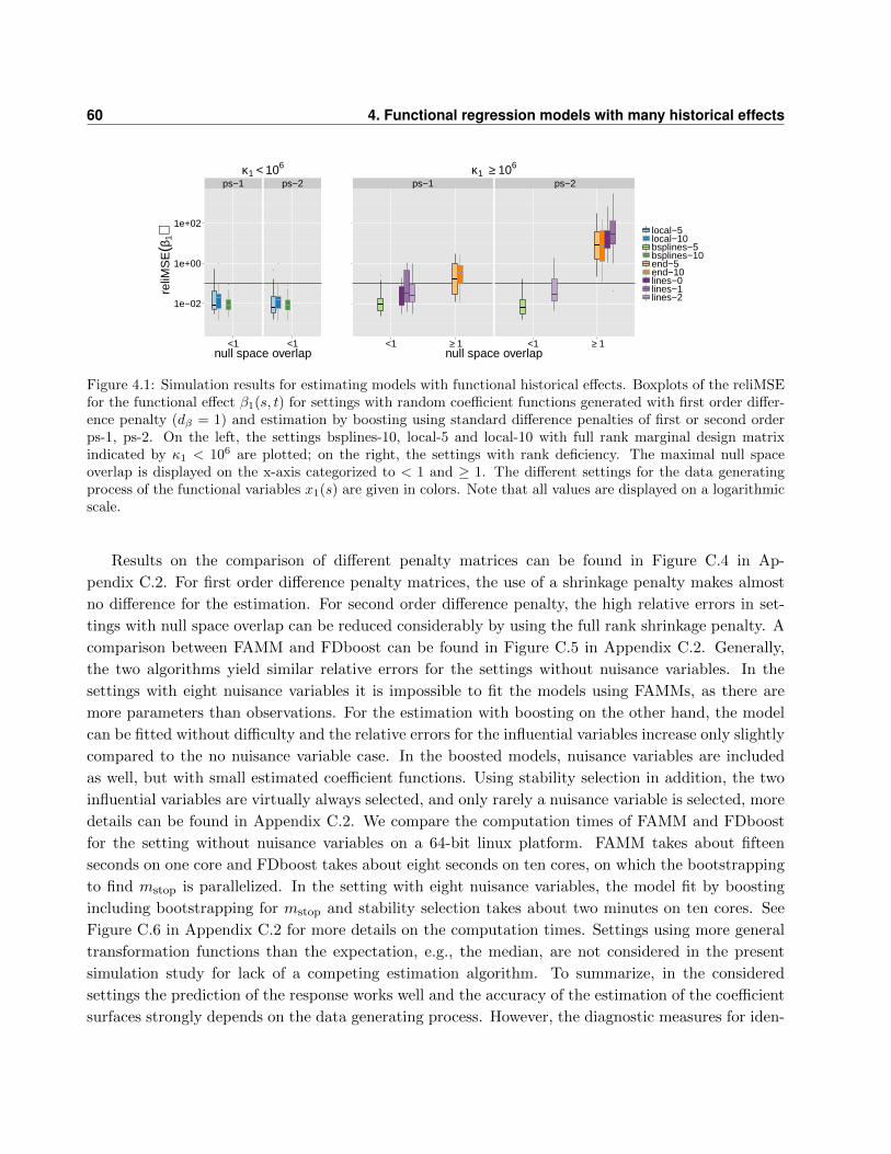
60 4. Functional regression models with many historical effects
ps−1 ps−2
●
●
●
●
●
1e−02
1e+00
1e+02
<1 <1null space overlap
reliM
SE
(β1)
κ1 < 106
ps−1 ps−2
●
●
<1 ≥ 1 <1 ≥ 1null space overlap
local−5local−10bsplines−5bsplines−10end−5end−10lines−0lines−1lines−2
κ1 ≥ 106
Figure 4.1: Simulation results for estimating models with functional historical effects. Boxplots of the reliMSEfor the functional effect β1(s, t) for settings with random coefficient functions generated with first order differ-ence penalty (dβ = 1) and estimation by boosting using standard difference penalties of first or second orderps-1, ps-2. On the left, the settings bsplines-10, local-5 and local-10 with full rank marginal design matrixindicated by κ1 < 106 are plotted; on the right, the settings with rank deficiency. The maximal null spaceoverlap is displayed on the x-axis categorized to < 1 and ≥ 1. The different settings for the data generatingprocess of the functional variables x1(s) are given in colors. Note that all values are displayed on a logarithmicscale.
Results on the comparison of different penalty matrices can be found in Figure C.4 in Ap-
pendix C.2. For first order difference penalty matrices, the use of a shrinkage penalty makes almost
no difference for the estimation. For second order difference penalty, the high relative errors in set-
tings with null space overlap can be reduced considerably by using the full rank shrinkage penalty. A
comparison between FAMM and FDboost can be found in Figure C.5 in Appendix C.2. Generally,
the two algorithms yield similar relative errors for the settings without nuisance variables. In the
settings with eight nuisance variables it is impossible to fit the models using FAMMs, as there are
more parameters than observations. For the estimation with boosting on the other hand, the model
can be fitted without difficulty and the relative errors for the influential variables increase only slightly
compared to the no nuisance variable case. In the boosted models, nuisance variables are included
as well, but with small estimated coefficient functions. Using stability selection in addition, the two
influential variables are virtually always selected, and only rarely a nuisance variable is selected, more
details can be found in Appendix C.2. We compare the computation times of FAMM and FDboost
for the setting without nuisance variables on a 64-bit linux platform. FAMM takes about fifteen
seconds on one core and FDboost takes about eight seconds on ten cores, on which the bootstrapping
to find mstop is parallelized. In the setting with eight nuisance variables, the model fit by boosting
including bootstrapping for mstop and stability selection takes about two minutes on ten cores. See
Figure C.6 in Appendix C.2 for more details on the computation times. Settings using more general
transformation functions than the expectation, e.g., the median, are not considered in the present
simulation study for lack of a competing estimation algorithm. To summarize, in the considered
settings the prediction of the response works well and the accuracy of the estimation of the coefficient
surfaces strongly depends on the data generating process. However, the diagnostic measures for iden-
4.6 Application in bioprocess monitoring 61
tifiability work well in flagging problematic settings where high relative errors occur. In settings with
rank deficient design matrix the estimation is still reasonably good if no null space overlap occurs.
Our proposed approach yields similar results to the competitor FAMM in settings where FAMM can
be applied and still yields good results in settings with more parameters than observations, where
FAMM cannot be used.
4.6 Application in bioprocess monitoring
The aim of this study is the monitoring of the cell dry mass (CDM, measured in g) during a biotech-
nological fermentation for the production of a model protein. Traditionally the CDM is determined
offline (i.e., by taking and analyzing a sample in the laboratory) according to a time-consuming
multi-step protocol, which prevents an early fault diagnosis in the process. Consequently, an online
prediction of the CDM based on easily accessible physical and/or chemical process variables or sensor
signals would be desirable. The dataset at hand is derived from 18 fermentations performed within
a full factorial design with factors temperature (two levels), growth rate (three levels) and induction
strength (three levels). Furthermore, a historical dataset with four fermentations and three duplicates
is available, yielding N = 25 fermentations in total. The CDM was determined on an approximately
hourly basis resulting in about 480 irregularly spaced observations in total. As time variable we use
the estimated number of generations of the Escherichia coli bacteria. Prediction of the CDM shall be
based on three types of online sensor signals serving as explanatory variables:
Process Data (PD): a set of 7 variables providing physical information on the process: air flow,
head pressure, dissolved O2, CO2 and O2 in the exhaust gas, feed and base consumption.
BioView R© Data (BV): a set of 120 variables containing fluorescence intensities I (λex, λem) mea-
sured for a pair of excitation/emission wavelengths (λex, λem) with λex ranging from 270 to
550 nm and λem from 310 to 590 nm. Additionally, 30 variables of type I (exnd, λem) or
I (λex, emnd) provide information on the scattering properties of the medium by using a neutral
density (nd) filter either in excitation- or in emission-mode (Melcher et al., 2015).
PTR-MS Data (PTR): a set of 22 variables with the cumulative amount and formation (or con-
sumption) rates measured for 11 mass numbers (substances) by proton-transfer-reaction mass
spectrometry (Luchner et al., 2012).
Only BV variables are used that have a correlation of at most 0.95 with other BV variables, leaving
32 BV variables in the analysis, see Melcher et al. (2015) for details. The data preprocessing for
the online measured covariates covers smoothing, time alignment, centering and scaling, resulting in
covariates with 202 observations per curve, details can be found in Appendix C.3. In Figure 4.2, the
response variable CDM is plotted. In each plot the same two fermentations are highlighted, namely
SOD42 in red and SOD62 in turquoise, using the same labels for the fermentations as Melcher et al.
(2015).

62 4. Functional regression models with many historical effects
5 10 15
100
200
300
400
generation
CD
M
Figure 4.2: Data on fermentation processes. Plot of the response variable CDM versus the generation time.
Model specification. Since the PD variables are routinely measured they can be used without
extra cost in all models. To measure the BV and the PTR variables additional instruments are
necessary and hence it is of practical interest to check for the added benefit of those variables for
the prediction of the outcome. We fit models using the PD, the PD-BV or the PD-PTR variables as
covariates. The used historical model is
E(Yi(t)|xi) = β0(t) +
J∑j=1
∫ t
T1
xij(s)βj(s, t) ds, (4.11)
where E is the expectation (boosting could alternatively fit the median or some quantile), Yi(t) is
the response at generation t, t ∈ [1.2, 16.4], for fermentation i, i = 1, . . . , 25, xi is the vector of all
covariates, xij(s) is the observation of functional covariate j for fermentation i at generation s and
βj(s, t) is the coefficient surface of covariate j with triangular support. Additionally, we fit a stan-
dardized historical model, see equation (4.5), where each functional historical effect is standardized
by the length of the integration interval:
E(Yi(t)|xi) = β0(t) +J∑j=1
1
t− T1
∫ t
T1
xij(s)βj(s, t) ds. (4.12)
As in our application the range of the response is growing over time, see Figure 4.2, it seems more
adequate to use the historical effects without standardization, equation (4.11). In this model a
constant coefficient surface and a constant covariate induce a partial effect that is growing or falling

4.6 Application in bioprocess monitoring 63
linearly, as the length of the integration interval is increasing. To investigate the benefit of using the
history of the covariates, we also fit the concurrent model
E(Yi(t)|xi) = β0(t) +
J∑j=1
xij(t)βj(t), (4.13)
where βj(t) is the concurrent effect of the jth covariate on the response. In the historical models the
effects are represented by using Kj = KY = 8 cubic B-splines as marginal bases in s and t direction
(see Section 4.2, equation (4.3)). For the concurrent effect, the marginal basis is bj(x, t)> = x(t)
and we use the same bY (t) as for the historical effects. For all base-learners, we specify five degrees
of freedom, inducing different values for λj . As in the simulation study results were most stable
for first order difference penalties, we use squared first order difference matrices as marginal penalties.
Tuning parameters and goodness of prediction. The same methods are used to determine the
optimal stopping iteration in the boosting algorithm and to assess the predictive power of the
models. We search the optimal mstop in the values {1, 2, . . . , 2000} for fixed step-size ν = 0.1. To
find the optimal stopping iteration we use leaving-one-curve-out-cross-validation (CCV). That means
the model is fitted using all curves but one and the left out curve is used as evaluation data. The
prediction for the left-out curve yi(t) is denoted by y(−i)i (t). To take into account the functional
character of the data, we integrate the loss per trajectory and standardize it with the length of the
trajectories,
funMeanLoss =1
N
N∑i=1
1
|T |
∫Tρ(yi, y
(−i)i
)(t) dt.
As loss function we use the squared error loss ρL2(y, y) = (y − y)2, which yields the functional mean
squared error (funMSE). For easier interpretation, we use the root mean squared error (funRMSE),
defined as√
funMSE.
Variable selection. As many covariates are available, variable selection is crucial. The result-
ing model using CCV often contains many variables, but some base-learners contribute only small
effects to the prediction of the outcome and are selected quite rarely. To obtain more parsimonious
models only containing important effects, we conduct complementary pairs stability selection (Shah
and Samworth, 2013), see Section 4.4. We set the threshold πthr = 0.9 and the PFER to < 0.1 · J ,
for J base-learners in the model, this induces q to be 3, 19 and 14 in the models with intercept
plus the 7 PD variables, 39 PD-BV variables and 29 PD-PTR variables, respectively. The PFER is
controlled under the assumptions that the variable selection of boosting works better than random
guessing and that the selection of noise variables is exchangeable. Both assumptions are difficult to
check in practice. Without relying on those assumptions the complementary pairs stability selection
controls the expected number of low selection probability variables. As the major interest lies in
finding a good prediction model and we use stability selection mainly for ordering the variables, we
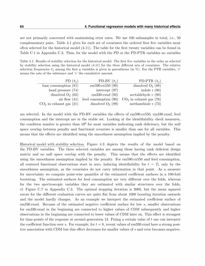
64 4. Functional regression models with many historical effects
are not primarily concerned with maintaining error rates. We use 100 subsamples in total, i.e., 50
complementary pairs. Table 4.1 gives for each set of covariates the ordered first five variables most
often selected for the historical model (4.11). The table for the first twenty variables can be found in
Table C.1 in Appendix C.3. Thus, for the model with the PD or the PD-PTR variables no variables
Table 4.1: Results of stability selection for the historical model. The first five variables in the order as selectedby stability selection using the historical model (4.11) for the three different sets of covariates. The relativeselection frequencies πj among the first q variables is given in parentheses (in %). For the PTR variables, ’r’means the rate of the substance and ’c’ the cumulative amount.
PD (πj) PD-BV (πj) PD-PTR (πj)
base consumption (81) em590.ex550 (99) dissolved O2 (88)head pressure (74) intercept (97) indole r (86)dissolved O2 (62) em330.exnd (92) acetaldehyde c (80)
air flow (41) feed consumption (90) CO2 in exhaust gas (76)CO2 in exhaust gas (21) dissolved O2 (89) methanthiole r (73)
are selected. In the model with the PD-BV variables the effects of em590.ex550, em330.exnd, feed
consumption and the intercept are in the stable set. Looking at the identifiability check measures,
the condition number is greater than 106 for most variables indicating rank deficiency, but the null
space overlap between penalty and functional covariate is smaller than one for all variables. This
means that the effects are identified using the smoothness assumption implied by the penalty.
Historical model with stability selection. Figure 4.3 depicts the results of the model based on
the PD-BV variables. The three selected variables are among those having rank deficient design
matrix and no null space overlap with the penalty. This means that the effects are identified
using the smoothness assumption implied by the penalty. For em590.ex550 and feed consumption,
all centered functional observations start in zero, inducing identifiability for t = T1 only by the
smoothness assumption, as the covariates do not carry information in that point. As a measure
for uncertainty we compute point-wise quantiles of the estimated coefficient surfaces in a 100-fold
bootstrap. The estimated surfaces for feed consumption are very different over the folds, whereas
for the two spectroscopic variables they are estimated with similar structures over the folds,
cf. Figure C.7 in Appendix C.3. The optimal stopping iteration is 2000, but the mean squared
errors for the different evaluation curves are quite flat from about 1000 boosting iteration onwards
and the model hardly changes. As an example we interpret the estimated coefficient surface of
em330.exnd. Because of the estimated negative coefficient surface for low s, smaller observations
for em330.exnd in the beginning are connected to higher values of CDM subsequently and higher
observations in the beginning are connected to lower values of CDM later on. This effect is strongest
for time-points of the response at around generation 13. Fixing a certain value of t one can interpret
the coefficient function over s. For example, for t = 8, recent values of em330.exnd have a strong posi-
tive association with CDM but this effect decreases for smaller values of s and even becomes negative.
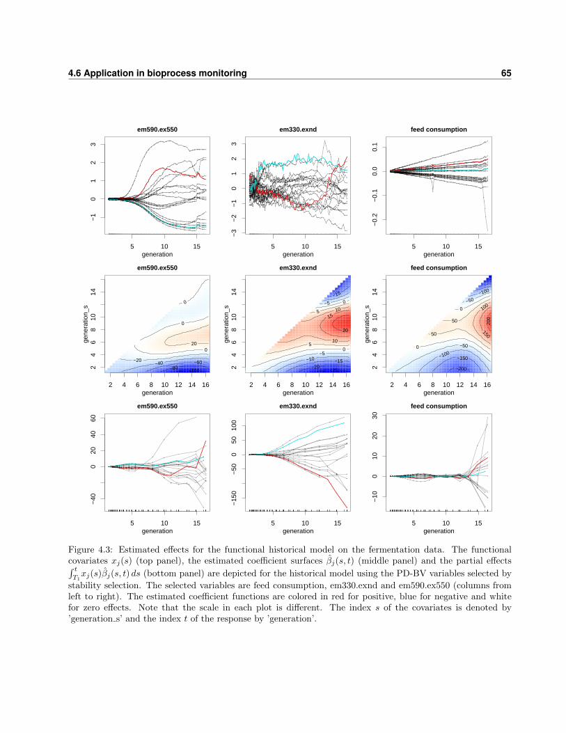
4.6 Application in bioprocess monitoring 65
5 10 15
−1
01
23
em590.ex550
generation5 10 15
−3
−2
−1
01
23
em330.exnd
generation5 10 15
−0.
2−
0.1
0.0
0.1
feed consumption
generation
2 4 6 8 10 12 14 16
24
68
1014
em590.ex550
generation
gene
ratio
n_s
−100 −80 −60 −40 −20
0
0
0
20
2 4 6 8 10 12 14 16
24
68
1014
em330.exnd
generation
gene
ratio
n_s
−25 −20 −15
−15
−10 −5
−5
0
0
5
5
10
10
15
20
2 4 6 8 10 12 14 16
24
68
1014
feed consumption
generation
gene
ratio
n_s
−200
−150 −100
−100
−50
−50
0
0
50
50
100
150
200
5 10 15
−40
020
4060
em590.ex550
generation5 10 15
−15
0−
500
5010
0
em330.exnd
generation5 10 15
−10
010
2030
feed consumption
generation
Figure 4.3: Estimated effects for the functional historical model on the fermentation data. The functionalcovariates xj(s) (top panel), the estimated coefficient surfaces βj(s, t) (middle panel) and the partial effects∫ tT1xj(s)βj(s, t) ds (bottom panel) are depicted for the historical model using the PD-BV variables selected by
stability selection. The selected variables are feed consumption, em330.exnd and em590.ex550 (columns fromleft to right). The estimated coefficient functions are colored in red for positive, blue for negative and whitefor zero effects. Note that the scale in each plot is different. The index s of the covariates is denoted by’generation s’ and the index t of the response by ’generation’.
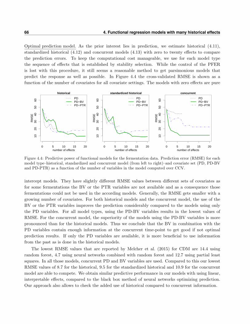
66 4. Functional regression models with many historical effects
Optimal prediction model. As the prior interest lies in prediction, we estimate historical (4.11),
standardized historical (4.12) and concurrent models (4.13) with zero to twenty effects to compare
the prediction errors. To keep the computational cost manageable, we use for each model type
the sequence of effects that is established by stability selection. While the control of the PFER
is lost with this procedure, it still seems a reasonable method to get parsimonious models that
predict the response as well as possible. In Figure 4.4 the cross-validated RMSE is shown as a
function of the number of covariates for all covariate settings. The models with zero effects are pure
0 5 10 15 20
1020
3040
5060
historical
number of effects
RM
SE
PDPD−BVPD−PTR
0 5 10 15 20
1020
3040
5060
standardized historical
number of effects
RM
SE
PDPD−BVPD−PTR
0 5 10 15 20
1020
3040
5060
concurrent
number of effects
RM
SE
PDPD−BVPD−PTR
Figure 4.4: Predictive power of functional models for the fermentation data. Prediction error (RMSE) for eachmodel type–historical, standardized and concurrent model (from left to right)–and covariate set (PD, PD-BVand PD-PTR) as a function of the number of variables in the model computed over CCV.
intercept models. They have slightly different RMSE values between different sets of covariates as
for some fermentations the BV or the PTR variables are not available and as a consequence those
fermentations could not be used in the according models. Generally, the RMSE gets smaller with a
growing number of covariates. For both historical models and the concurrent model, the use of the
BV or the PTR variables improves the prediction considerably compared to the models using only
the PD variables. For all model types, using the PD-BV variables results in the lowest values of
RMSE. For the concurrent model, the superiority of the models using the PD-BV variables is more
pronounced than for the historical models. Thus we conclude that the BV in combination with the
PD variables contain enough information at the concurrent time-point to get good if not optimal
prediction results. If only the PD variables are available, it is more beneficial to use information
from the past as is done in the historical models.
The lowest RMSE values that are reported by Melcher et al. (2015) for CDM are 14.4 using
random forest, 4.7 using neural networks combined with random forest and 12.7 using partial least
squares. In all those models, concurrent PD and BV variables are used. Compared to this our lowest
RMSE values of 8.7 for the historical, 9.5 for the standardized historical and 10.9 for the concurrent
model are able to compete. We obtain similar predictive performance in our models with using linear,
interpretable effects, compared to the black box method of neural networks optimizing prediction.
Our approach also allows to check the added use of historical compared to concurrent information.
4.7 Discussion 67
4.7 Discussion
In this chapter, we focus on regression models with a large number of functional historical effects,
which are function-on-function effects where the support of the coefficient surface is constrained to a
certain area. The implementation is such that arbitrary lower and upper integration limits {l(t), u(t)}can be specified as functions of t for a functional response Y (t). In particular, historical effects with
integration limits {T1, t} and lag models with integration limits {t−δ, t} can be fitted. The introduced
reparameterizations of historical effects, accounting for the differing length of the integration interval,
can be useful for applications in which the response has a similar range over time. Additionally,
hybrid models combining different kinds of effects can be estimated. In our application, for example,
we fitted a hybrid model with concurrent effects of the BV and historical effects of the PD variables
(results not shown).
In contrast to black-box prediction algorithms, such as neural networks, our models provide inter-
pretable results as illustrated by the estimated coefficient functions in the historical model for CDM
while in many cases being competitive in terms of prediction. We obtained the best prediction models
for CDM using the process and the spectroscopic variables (PD-BV) as historical or concurrent ef-
fects. If only the process data (PD) are used, the historical models yield considerably lower prediction
errors than the concurrent models.
We embed the historical models in a more general framework for boosting functional regression
models that (a) allows to model not only the conditional mean of the response but also other features
of the conditional distribution for (b) functional responses observed on equal or unequal grids, (c)
includes the possibility to specify many different effects, in particular functional historical effects, (d)
can estimate models with a great number of covariate effects, and (e) inherently does variable selection.
We understand our framework as a toolbox for functional regression that easily allows to estimate
models under different assumptions or with differing effects. For example, it is straightforward to use
the robust absolute error loss instead of the squared error loss, replacing mean by median regression.
In the R add-on package FDboost, we provide a comprehensive implementation that should lower the
hurdle for practitioners to use functional regression models.
The methods can be applied to other fields collecting functional data, e.g., financial or clinical
data. The framework for functional historical models could be extended into several directions. For
some applications, it may be of interest to develop a method that identifies important regions in
each coefficient surface within the fitting procedure and sets the remaining surface to zero; see Tutz
and Gertheiss (2010) for feature extraction with boosting for scalar-on-function regression. It may
also be of interest to extend the linear functional historical effect to non-linear effects, cf. Scheipl
et al. (2015), which might further improve predictive performance in some cases. Such a model would
require larger sample sizes than in our case study and careful investigation of identifiability.
Acknowledgments
Special thanks to Markus Luchner and Gerald Striedner for providing us with the fermentation data.
We thank Fabian Scheipl for useful discussions. The work of Sarah Brockhaus and Sonja Greven was

68 4. Functional regression models with many historical effects
supported by the German Research Foundation (DFG) through Emmy Noether grant GR 3793/1-1.
The work of Michael Melcher and Friedrich Leisch was supported by the Federal Ministry of Traffic,
Innovation and Technology (bmvit), the Federal Ministry of Economy, Family and Youth (BMWFJ),
the Styrian Business Promotion Agency (SFG), the Standortagentur Tirol and the ZIT Technology
Agency of the City of Vienna through the COMET-Funding Program managed by the Austrian
Research Promotion Agency (FFG). The computational results presented have been in part achieved
using the Vienna Scientific Cluster (VSC). We thank the reviewers and the associate editor for their
useful comments.
Chapter 5
Signal regression models for location,
scale and shape
Contributing manuscript
This chapter is based on the following preprint:
Brockhaus, S., Fuest, A., Mayr, A. and Greven, S. (2016): Signal regression mod-
els for location, scale and shape with an application to stock returns. arXiv preprint,
arXiv:1605.04281.
This is joint work with Andreas Fuest (Department of Statistics, LMU Munich, Germany), An-
dreas Mayr (Department of Medical Informatics, Biometry and Epidemiology, Friedrich-Alexander-
University Erlangen-Nurnberg, Germany) and Sonja Greven (Department of Statistics, LMU Munich,
Germany). The idea for this paper came out of Andreas Mayr’s and Sarah Brockhaus’ thought to
combine their work, resulting in the combination of boosting GAMLSS (Mayr et al., 2012) and
boosting functional regression models. The idea became a project when Andreas Fuest added the
application to a time series of stock returns, in which the focus lies on modeling the variance of the
response. Andreas Fuest contributed the knowledge and literature on time series analysis, proposed
the models that were used for the data analysis and wrote the part of the application section explain-
ing the dataset (beginning of Section 5.8). Sarah Brockhaus performed all analysis, including the
simulation study and the data analysis, and drafted the manuscript. Andreas Mayr contributed to
the understanding of boosting GAMLSS and the implementation in the R package gamboostLSS. The
methodological developments to include functional effects into GAMLSS were conducted by Sarah
Brockhaus in cooperation with the other authors. Sonja Greven contributed to the structure and the
revision of the paper. All coauthors gave feedback on the manuscript.
A short, early version of Chapter 5 can be found in the conference proceedings of IWSM 2015 (30th
International Workshop on Statistical Modelling), see Brockhaus et al. (2015a).
70 5. Signal regression models for location, scale and shape
Software
The analyses in this chapter were conducted by R version 3.2.3 (R Core Team, 2015). For boosting
functional regression models, the R packages FDboost 0.0-16 (Brockhaus and Rugamer, 2016), mboost
2.5-0 (Hothorn et al., 2016) and gamboostLSS 1.2-0 (Hofner et al., 2015b) were used. For penalized
maximum likelihood-based estimation of GAMLSS with functional covariates, we used the packages
gamlss 4.3-8 (Stasinopoulos et al., 2016), gamlss.add 4.3-4 (Rigby and Stasinopoulos, 2015) and mgcv
1.8-11 (Wood, 2016).
5.1 Introduction
The field of functional data analysis (Ramsay and Silverman, 2005) deals with the special data
situation where the observation units are curves. The functions have continuous support, e.g., time,
wavelength or space. One typically assumes that the true underlying functions are smooth and
theoretically the functions could be measured on arbitrarily fine grids, even though in practice the
functions are measured at a finite number of discrete points. Due to technical progress, more and more
data sets containing functional variables are available. Regression methods for functional data are of
increasing interest and have been developed for functional responses and/or functional covariates; see
Morris (2015) for a recent review on regression methods with functional data.
In this chapter, we consider a case study on returns for the stocks of Commerzbank from November
2008 to December 2010 (Fuest and Mittnik, 2015). The primary interest lies in predicting the variances
of the stock returns whereas the modeling of the expectation is only of secondary interest, as it is a
well-known empirical fact that the latter is hardly predictable. In contrast, the conditional variance is
typically time-varying and strongly serially correlated (see, e.g., Cont, 2001). Apart from the returns,
however, our data set includes rich information on the market participants’ offers and requests as
potential predictors, which we use as covariates in the form of liquidity curves. Consequently, we
want to fit a regression model for the expectation and the variance of a scalar response using several
functional and scalar covariates.
So far, most publications dealing with scalar-on-function regression have focused on modeling the
conditional expectation. The linear functional model was introduced by Ramsay and Dalzell (1991)
yi = β0 +
∫Sxi(s)β(s) + εi, (5.1)
with continuous response yi, i = 1, . . . , N , functional covariate xi(s), s ∈ S, with S a closed interval
in R, intercept β0, functional coefficient β(s) and errors εiiid∼ N(0, σ2). Many extensions of this model
have been proposed, concerning the response distribution, non-linearity of the effect and inclusion
of further covariate effects. For non-normal responses, generalized linear models (GLMs, Nelder and
Wedderburn, 1972) with linear effects of functional covariates (e.g., Marx and Eilers, 1999; Ramsay
and Silverman, 2005; Muller and Stadtmuller, 2005; Goldsmith et al., 2011) and generalized additive
models (GAMs, Hastie and Tibshirani, 1986) with non-linear effects of functional covariates (e.g.,

5.1 Introduction 71
James and Silverman, 2005; McLean et al., 2014) have been discussed. As distribution-free approach
quantile regression (Koenker, 2005) with functional covariates has been considered, see, e.g., Ferraty
et al. (2005); Cardot et al. (2005); Chen and Muller (2012a). The most important differences between
those models are the choice of the basis representation for the functional covariate and/or the func-
tional coefficient, and the choice of the fitting algorithm. Common choices for the bases are functional
principal components and splines. The estimation is mostly done by (penalized) maximum likelihood
approaches. However, functional regression models that model simultaneously several parameters of
the conditional response distribution have not been considered. This can be overcome in the frame-
work of generalized additive models for location, scale and shape (GAMLSS), introduced by Rigby
and Stasinopoulos (2005), where all distribution parameters can be modeled depending on covariates.
For estimation, Newton-Raphson or Fisher-Scoring is used to maximize the (penalized) likelihood.
Mayr et al. (2012) estimate GAMLSS in high-dimensional data settings by a component-wise gradient
boosting algorithm. Klein et al. (2015) discuss Bayesian inference for GAMLSS and denominate the
model as structured additive distributional regression, as the modeled distribution parameters are not
necessarily location, scale and shape but rather determine those characteristics indirectly. Inference
is based on a Markov chain Monte Carlo simulation algorithm with distribution-specific iteratively
weighted least squares approximations for the full conditionals. For each of these three approaches,
complex parametric distributions like the (inverse) Gaussian, Weibull or Negative Binomial distribu-
tion can be assumed for the response variable. None of these three papers discusses the incorporation
of functional covariates into GAMLSS.
Wood et al. (2015) propose an estimation framework for smooth models with (non-)exponential
families, including certain GAMLSS as special case. In the current implementation three response
distributions for GAMLSS–a normal location scale, a two-stage zero-inflated Poisson and a multino-
mial logistic model–are available. The focus lies on stable smoothing parameter estimation and model
selection. Already in an earlier paper, Wood (2011) discusses how to incorporate linear functional
effects into GAMs using spline expansions of β(s) and Wood et al. (2015) includes an example of a
model with ordered categorical response and one functional covariate. The functional model terms
can be included in the mentioned GAMLSS within the implementation in R package mgcv, using
R software for statistical computing. Thus, scalar-on-function models for normal location scale, two-
stage zero-inflated Poisson and multinomial logistic models are available in the implementation, but
have not been discussed so far.
In this chapter, we discuss the extension of scalar-on-function regression models in the spirit of
GAMLSS and denominate these models as signal regression models for location, scale and shape. We
address practically important points like identifiability and model choice and compare different esti-
mation methods. The signal regression terms are specified as in Wood (2011) and in Chapter 3. The
second allows in addition to linear functional effects as in (5.1) interaction terms zi∫S xij(s)βj(s) ds
or∫S xij(s)βj(s, zi) ds between scalar zi and functional xij(s) covariates. The functional coefficients
βj(s) can be expanded in a spline basis, such as P-splines (Eilers and Marx, 1996), or in the ba-
sis spanned by the functional principal components (FPCs, see, e.g., Ramsay and Silverman, 2005,
chap. 8) of the functional covariate. Representing the functional covariate and coefficient in FPCs,
72 5. Signal regression models for location, scale and shape
the scores of the FPCs are used like scalar covariates; see Section 5.3.1 where we will compare and
discuss different choices of basis functions. We propose and compare two fundamentally different
estimation approaches, based on gradient boosting (Mayr et al., 2012) and (penalized) maximum
likelihood (Rigby and Stasinopoulos, 2005; Wood et al., 2015). No estimation method is generally
superior, as each is suited to particular situations, as will be discussed in this chapter. Boosting
allows for high-dimensional data settings with more covariate effects than observations and variable
selection, but does not provide direct statistical inference. The maximum likelihood approaches imply
the usual machinery of statistical inference but are not applicable in high-dimensional data settings.
The combination of scalar-on-function regression and GAMLSS is motivated by the application
on stock returns but covers a much broader range of response distributions and functional effects.
The stock returns are a continuous real-valued response and we will use normal and t location scale
models. We model the linear functional effects for the liquidity curves using P-splines or FPC bases.
The remainder of the chapter is structured as follows: in Section 5.2 we formulate the GAMLSS
including functional effects. In Section 5.3 we give details on possible covariate effect terms, focusing
on effects of functional variables. In Section 5.4 the gradient boosting approach is presented. In
Section 5.5 we present estimation by penalized maximum likelihood, commenting on the gamlss-
algorithms by Rigby and Stasinopoulos (2005, 2014) and the smooth regression models by Wood
et al. (2015). A comparison between the estimation methods highlighting pros and cons is given in
Section 5.6. In Section 5.7 we comment on criteria for model choice. Section 5.8 shows the analysis
of the log-return data assuming a normal or t-distribution for the response and using functional
liquidity curves as covariates. In Section 5.9 we present results of two simulation studies–the first is
closely related to the application; the second systematically compares the three discussed estimation
algorithms. We conclude in Section 5.10 with a short discussion and an outlook on future research.
In the Appendix D, we give details on the implementation of the methods in R including example
code for a small simulated dataset. Further results of the application and the simulation study as
well as reproducible code are given in Appendix D.
5.2 Generic model
We observe data-pairs from (Y,X) assuming that Y given X follows a conditional distribution FY |Xand X can be fixed or random. Let the response Y ∈ R and scalar covariates in R and functional
covariates in L2(S), where L2 is the space of square integrable functions on the real interval S =
[S1, S2], with S1 < S2 ∈ R. If there are several functional covariates, they can have differing domains.
One functional covariate is denoted by Xj(s), with s ∈ S. We denote the observed data by (yi, xi),
i = 1, . . . , N , and an observed functional covariate by xij(s), with observation points s ∈ (s1, . . . , sR)>,
sr ∈ S, which are equal for the i = 1, . . . , N observed trajectories. In general, random variables

5.2 Generic model 73
are denoted by upper and realizations by lower case. To represent a GAMLSS for Q distribution
parameters (Rigby and Stasinopoulos, 2005), the additive regression model has the general form
g(q)(ϑ(q)) = ξ(q)(Y |X = x) = h(q)(x) =J(q)∑j=1
h(q)j (x), q = 1, . . . , Q, (5.2)
where ϑ(q) is the qth distribution parameter of the response distribution and g(q) is the corresponding
link function relating the distribution parameter to its linear predictor h(q)(x). Equivalently, we use
a transformation function ξ(q), which is the composition of the function yielding the qth parameter
of the conditional response distribution and the link function g(q). To represent a GLM the model
contains only one equation, Q = 1, for the expectation, ϑ(1) = µ, and the transformation function is
the composition of the expectation E and the link function g(1), i.e. ξ(1) = g(1) ◦ E. More generally,
each function in the vector of transformation functions is the composition of a parameter function
and a link function. For example, for normally distributed response, the transformation functions
can be the expectation composed with the identity link, ξ(1) = E, and the variance composed with
the log link, ξ(2) = log ◦V. The framework allows for many different response distributions, including,
e.g., the (inverse) normal, t-, and gamma distribution. See Rigby and Stasinopoulos (2005) for an
extensive list of response distributions.
The linear predictor for the qth parameter, h(q), is the additive composition of covariate effects
h(q)j . Each effect h
(q)j (x) can depend on one covariate for simple effects or on a subset of covariates in x
to form interaction effects. Linear, non-linear and interaction effects of scalar covariates are possible
in the GAMLSS proposed by Rigby and Stasinopoulos (2005), Mayr et al. (2012), Klein et al. (2015)
and Wood et al. (2015). The latter allows additionally for linear functional effects, but is in the
current implementation restricted to three distribution families (considering only GAMLSS models).
We extend the existing models by allowing for linear functional effects and interaction terms between
scalar and functional covariates for general response distributions. Table 5.1 gives an overview on
possible covariate effects.
Table 5.1: Overview of possible covariate effects that can be specified in the linear predictors.
covariate(s) type of effect h(q)j (x)
(none) intercept β0
scalar variable z1 linear effect z1βsmooth effect f(z1)
plus scalar z2 linear interaction z1z2βsmooth interaction f(z1, z2)
grouping variable g group-specific smooth intercept βgplus scalar z group-specific linear effect zβg
functional variable x(s) linear functional effect∫S x(s)β(s) ds
plus scalar z linear interaction z∫S x(s)β(s) ds
smooth interaction∫S x(s)β(z, s) ds

74 5. Signal regression models for location, scale and shape
In the following section, we discuss the setup for the effects, with a special emphasis on effects of
functional covariates.
5.3 Specification of effects
We represent smooth effects by basis expansions, representing each partial effect, h(q)j (x), as linear
term
h(q)j (x) = b
(q)j (x)>θ
(q)j , (5.3)
where b(q)j : X → RK
(q)j , with X being the space of the covariates X, is a vector of basis evaluations
depending on one or several covariates and θ(q)j is the vector of basis coefficients that is to be estimated.
The effects are regularized by a quadratic penalty term,
θ(q)>j P
(q)j (λ)θ
(q)j , (5.4)
which for most covariate effects is taken as P(q)j (λ) = λ
(q)j P
(q)j , with fixed penalty matrix P
(q)j
and smoothing parameter λ(q)j ≥ 0 from the vector of all smoothing parameters λ. Thus, the
design matrix for each effect contains rows of basis evaluations b(q)j (xi)
>, i = 1, . . . , N , and the
corresponding coefficients are regularized using the penalty matrix P(q)j (λ). For better readability,
we skip the superscript (q) in the following description of covariate effects.
For the effects of scalar covariates, we refer to Rigby and Stasinopoulos (2005), Mayr et al.
(2012) and Wood et al. (2015), where even more effects of scalar variables than those listed in
Table 5.1 are described. The specification of effects of functional covariates is discussed in the
following two subsections.
5.3.1 Signal regression terms
Let a functional covariate xj(s) with domain S be observed on a grid (s1, . . . , sR)>. For a linear
functional effect∫S xj(s)βj(s) ds, also called signal regression term, the integral is approximated
using weights ∆(s) from a numerical integration scheme (Wood, 2011) giving
bj(xj(s))> = [xj(s1) · · · xj(sR)] [Φj(s1) · · · Φj(sR)]>
=
[R∑r=1
xj(sr)Φ1(sr) · · ·R∑r=1
xj(sr)ΦKj (sr)
],
(5.5)
where xj(s) = ∆(s)xj(s) and Φj(s) is a vector of basis functions Φk(s), k = 1, . . . ,Kj , evaluated at s.
The penalty matrix P j is chosen as matching to the basis functions Φj , e.g., a squared difference
matrix for B-splines (Eilers and Marx, 1996).
5.3 Specification of effects 75
To model a linear interaction between a scalar covariate z and a functional covariate,
z∫S xj(s)βj(s) ds, the basis in (5.5) is multiplied by z. For a smooth interaction
∫S xj(s)βj(z, s) ds,
we use (Scheipl et al., 2015, and Chapter 3)
bj(xj(s), z)> = bj1(xj(s))
> � bj2(z)>, (5.6)
where � is the row tensor product, bj1(xj(s)) is defined as in (5.5) and bj2(z) = Φj(z) are spline basis
evaluations of the scalar covariate z. A suitable penalty matrix for such an effect can be constructed
as (Wood, 2006, Sec. 4.1.8)
P j(λ) = λj1(P j1 ⊗ IKj2
)+ λj2
(IKj1 ⊗ P j2
), (5.7)
where P j1 ∈ RKj1×Kj1 , and P j2 ∈ RKj2×Kj2 are appropriate penalty matrices for the marginal bases
bj1(xj(s)) and bj2(z), and λj1, λj2 ≥ 0 are smoothing parameters.
5.3.2 Choice of basis functions and identifiability
Spline bases. Assuming the coefficient function βj(s) to be smooth, the basis functions Φj for the
functional linear effect (5.5) can be chosen, for instance, as B-splines, natural splines or thin plate
regression splines. Depending on the chosen spline basis a suitable penalty matrix has to be selected.
According to the penalty different smoothness assumptions are implied. For example, using P-splines
(Eilers and Marx, 1996), i.e., B-splines with a squared difference matrix as penalty, it is possible to
penalize deviations from the constant line or the straight line using first or second order differences
in the penalty.
Spline based methods require functional observations on dense grids and thus, for sparse
grids they have to be imputed in a preprocessing step (see, e.g., Goldsmith et al., 2011). The
implementations in mgcv and FDboost require functional observations on one common grid.
Functional principal component basis. In functional data analysis, functional principal compo-
nent analysis (FPCA, see, e.g., Ramsay and Silverman, 2005) is a common tool for dimension
reduction, and also widely used in functional regression analysis to represent the functional covariates
and/or the functional coefficients (cf., Morris, 2015). Let Xj(s) be a zero-mean square-integrable
stochastic process and ek(s) the eigenfunctions of the auto-covariance of Xj(s), with the respective
decreasing eigenvalues ζ1 ≥ ζ2 ≥ · · · ≥ 0. Then {ek(s), k ∈ N} form an orthonormal basis for the
L2(S) and the Karhunen-Loeve theorem states that
Xij(s) =∞∑k=1
Zikek(s),
where Zik are uncorrelated random variables with mean zero and variance ζk. This means that
functional observations xij(s) can be represented as weighted sums of (estimated) eigenfunctions.
76 5. Signal regression models for location, scale and shape
The eigenfunctions represent the main modes of variation of the functional variable and are also
called functional principal components (FPCs). In practice, the sum is truncated at a certain number
of basis functions. For a fixed number of basis functions, the eigenfunctions are the set of orthonormal
basis functions that best approximate the functional observations (see, e.g., Ramsay and Silverman,
2005). Representing both the functional covariate and the functional coefficient by the eigenfunction
basis truncated at Kj ,
∫Sxij(s)βj(s) ds ≈
Kj∑k,l=1
∫Szikek(s)el(s)θl ds =
Kj∑k=1
zikθk, (5.8)
follows from the orthonormality of ek(s). This approach thus corresponds to a regression onto the
estimated first Kj FPC scores zik and interaction effects with other scalar covariates can be specified
straightforwardly. Regularization is usually achieved by using only the first few eigenfunctions
explaining a fixed proportion of total variability (cf., Morris, 2015), for example 99%. Additionally,
a penalty matrix can be used for regularization. The penalty P j = diag(1/ζ1, . . . , 1/ζKj ) assumes
decreasing and P j = diag(1, . . . , 1) equal importance of the eigenfunctions. If the functional covariate
is observed on irregular or sparse grids, it is advantageous to use an FPC basis as it can be estimated
directly from the data even in this case (Yao et al., 2005a). Statistical inference is usually done
conditional on the eigendecomposition and thus neglects the variability induced by the estimation of
the eigenfunctions and FPC scores (Goldsmith et al., 2013).
Implicit assumptions and identifiability. Using an FPC basis, βj(s) is assumed to lie in the
space spanned by the first Kj eigenfunctions and the estimation depends on the choice of the discrete
tuning parameter Kj . For the spline representation, βj(s) is assumed to be smooth and to lie within
the space spanned by the spline basis. In practice, those assumptions are hard to check. If almost all
variation of the functional covariate can be explained by the first few eigenfunctions, the covariate
carries only little information. In this case, identifiability problems can occur for a spline-based
approach (Scheipl and Greven, 2016) and the estimation of βj(s) might be dominated by the
smoothness assumption. When using an FPCA basis, the estimation is dominated by the assumption
that βj(s) lies in the span of the first Kj eigenfunctions, with the estimate highly sensitive to the
quality of the estimates of ek(s) as well as to the choice of Kj . Higher-order eigenfunctions are
usually relatively wiggly and the shape of βj(s) can thus change strongly when increasing Kj (see,
e.g., Crainiceanu et al., 2009).
5.4 Estimation by gradient boosting
In this section we discuss the estimation of GAMLSS by a gradient boosting algorithm as introduced
by Mayr et al. (2012) and implemented in the R package gamboostLSS. We expand the algorithms by
effects (5.5) and (5.6) for functional covariates that are available in the FDboost package.
5.4 Estimation by gradient boosting 77
Gradient boosting is a machine learning algorithm that aims at minimizing an expected loss
criterion along the steepest gradient descent (Friedman, 2001). The model is represented as the sum
of simple (penalized) regression models, which are called base-learners. In our case the base-learners
are the models for the effects h(q)j (x), as defined by (5.3) and (5.4). We use a component-wise gradient
boosting algorithm (see, e.g., Buhlmann and Hothorn, 2007), that iteratively fits each base-learner
to the negative gradient of the loss and only updates the best-fitting base-learner per step. Thus,
models for high-dimensional data settings with more covariates than observations can be estimated
and variable selection is done inherently, as base-learners that are never selected for the update are
excluded from the model.
Boosting minimizes the expected loss
h = arg minh
E ρ (Y,h(X)) ,
where h(X) = (h(1)(X), . . . , h(Q)(X))> and ρ : R×RQ → [0,∞) is the loss function. In practice, for
observed data (yi, xi), i = 1, . . . , N , the theoretical expectation is approximated by the sample mean,
yielding optimization of the empirical risk,
h = arg minh
1
N
N∑i=1
wi ρ (yi,h(xi)) , (5.9)
where wi are sampling weights that can be used in resampling methods like cross-validation or boot-
strapping. To estimate a GAMLSS via boosting, the negative log-likelihood of the response distribu-
tion is used as loss function (Mayr et al., 2012), i.e., ρ (yi,h(xi)) = −l(ϑi, yi), with the log-likelihood l
depending on the vector of distribution parameters ϑi = (ϑ(1)i , . . . , ϑ
(Q)i )>, with ϑ
(q)i = g(q)−1(h(q)(xi)),
and the response yi. We expand the framework that Mayr et al. (2012) developed for boosting
GAMLSS by base-learners for signal regression terms, cf. equation (5.5), and interaction terms be-
tween scalar and functional covariates, cf. equation (5.6). In detail, the following boosting algorithm
is used:
Algorithm: Gradient boosting for GAMLSS with functional covariates
Step 1: Define the bases b(q)j (x, t), their penalties P
(q)j (λ), j = 1, . . . , J (q), q = 1, . . . , Q, and the
weights wi, i = 1, . . . , N . Select a vector of step-lengths (ν(1), . . . , ν(Q))>, with ν(q) ∈ (0, 1), and
a vector of stopping iterations (m(1)stop, . . . ,m
(Q)stop)>. Initialize the coefficients θ
(q)[0]j .
Set the number of boosting iterations to zero, m = 0.
Step 2: (Iterations over the parameters of the response distribution, q = 1, . . . , Q)
(a) Set q = 1.

78 5. Signal regression models for location, scale and shape
(b) If m > m(q)stop go to step 2(g);
otherwise, compute the negative partial gradient of the empirical risk by plugging in the
current estimates h[m]
=(h(1)[m], . . . , h(Q)[m]
)>, with h(q)[m](xi) =
∑j b
(q)j (xi)θ
(q)[m]j , as
u(q)i = − ∂
∂h(q)ρ (yi,h(xi))
∣∣∣∣h(xi)=h
[m](xi)
.
(c) Fit the base-learners contained in h(q) for j = 1, . . . , J (q) to u(q)i :
γj = arg minγ∈RKj
N∑i=1
wi
{u
(q)i − b
(q)j (xi)
>γ}2
+ γ>P(q)j (λ)γ,
with weights wi and penalty matrices P(q)j (λ).
(d) Select the best fitting base-learner, defined by the least squares criterion:
j? = arg minj=1,...,J(q)
N∑i=1
wi
{u
(q)i − b
(q)j (xi)
>γj
}2.
(e) Update the corresponding coefficients of h(q)[m] to θ(q)[m]j? = θ
(q)[m]j? + ν(q)γj? .
(f) Set θ(q)[m+1]j = θ
(q)[m]j , j = 1, . . . , J (q).
(g) Unless q = Q, increase q by one and go back to step 2(b).
Step 3: Unless m ≥ m(q)stop for all q, increase m by one and go back to step 2.
Each component of the final model is a linear combination of base-learner fits ξ(q)(Yi|Xi = xi) =∑j h
(q)[m(q)stop]
j (xi). In order to get a fair model selection, we specify equal and rather low degrees
of freedom for all base-learners by using adequate values for the smoothing parameters λ(q)j (Kneib
et al., 2009; Hofner et al., 2011). Using additionally a small fixed number for the step-length, e.g.,
ν(q) = 0.1, for all q, the model complexity is controlled by the number of boosting iterations for
each distribution parameter. That means that the numbers of boosting iterations are used as the
only tuning parameters. The vector of stopping iterations is determined by resampling methods
like cross-validation or bootstrapping using the weights wi for the observations. Mayr et al. (2012)
distinguish between one-dimensional early stopping, that is m(q)stop ≡ mstop for q = 1 . . . , Q, and
multi-dimensional early stopping where the stopping iterations m(q)stop differ for q = 1 . . . , Q. Multi-
dimensional early stopping increases the computational effort, as the optimal stopping iterations are
searched on a Q-dimensional grid. In the following, we will use multi-dimensional early stopping as it
allows for different model complexities for each distribution parameter. Stopping the algorithm early
achieves shrinkage of the parameter effects and variable selection, as in each step only the best fitting
base-learner is updated.

5.5 Estimation based on penalized maximum likelihood 79
For low-dimensional data settings, i.e., “N > p”, and unpenalized estimation, the solution of the
boosting algorithm converges to the same solution as maximum likelihood estimation if the number of
boosting iterations goes to infinity for all distribution parameters. This can be shown using gradient
descent arguments (Rosset et al., 2004; Mayr et al., 2012).
5.5 Estimation based on penalized maximum likelihood
We review two estimation approaches that can be used to estimate GAMLSS by maximizing the
penalized likelihood. In contrast to component-wise boosting, where each effect is modeled in a
separate base-learner, for penalized likelihood estimation all effects of the linear predictors are es-
timated together using one likelihood. We first introduce some notation for this purpose. The
model coefficients θ(q)j , j = 1, . . . , J (q), for the qth distribution parameter are concatenated to the
vector θ(q), which are concatenated to the vector θ containing the model parameters of all linear
predictors. Analogously, the penalty matrix of all coefficients of the qth distribution parameter is
P (q)(λ) = blockdiag([P(q)j (λ)]j=1,...,J(q)), and the penalty matrix for the model coefficients of all lin-
ear predictors is P (λ) = blockdiag([P (q)(λ)]q=1,...,Q). The generalized inverse of the penalty matrix
is denoted by P (λ)−. We call the vector of all smoothing parameters λ = (λ(1)1 , . . . , λ
(Q)
J(Q))>. For
fixed smoothing parameters λ, the model coefficients θ are estimated by maximizing the penalized
log-likelihood (see, e.g., Rigby and Stasinopoulos, 2005; Wood et al., 2015)
lp(θ) = l(ϑ, y)− 1
2θ>P (λ)θ, (5.10)
where l(ϑ, y) =∑N
i=1 log f(yi, ϑ(1)i , . . . , ϑ
(Q)i ) is the log-likelihood of the data given the distribution
parameters and the distribution parameters ϑ depend on the model coefficients θ.
Generally, there are two different approaches to find the optimal smoothing parameters λ. The
first approach is to minimize a model prediction error, for example, a generalized Akaike information
criterion (GAIC) or a generalized cross-validation criterion (GCV). The second approach is to use
the random effects formulation, where the smoothness penalties can be seen as induced by improper
Gaussian priors on the model parameters θ, as θ ∼ N(0, P (λ)−). The smoothing parameters λ can
then be estimated by maximizing the marginal likelihood with respect to the smoothing parameters.
The marginal likelihood is obtained by integrating the model parameters θ out of the joint density of
the data and the model parameters (Patterson and Thompson, 1971; Wood et al., 2015),
Vr(λ) =
∫exp [l(ϑ, y)] fλ(θ) dθ, (5.11)
where fλ(θ) is the density of the Gaussian prior N(0,P (λ)−). For the normal distribution, maximiz-
ing this marginal likelihood is equivalent to maximizing the restricted likelihood (REML). A common
approach for maximization is to approximate the integral by Laplace approximation, resulting in the
Laplace approximate marginal likelihood (LAML).
80 5. Signal regression models for location, scale and shape
5.5.1 The gamlss algorithm using backfitting
Rigby and Stasinopoulos (2005) first introduced the model class GAMLSS and proposed several
variants of a backfitting algorithm for estimation. They provide an implementation for many different
response distributions, which at the moment lacks the possibility to specify effects of functional
covariates. However, the implementation in R package gamlss allows to specify linear functional
effects (5.5) as proposed by Wood (2011) using the gamlss.add package to incorporate smooth terms
of the mgcv package.
In the fitting algorithm, iterative updates of the smoothing parameters λ and the model coeffi-
cients θ are computed. Estimation of the smoothing parameters λ is done by maximizing the marginal
likelihood or minimizing a model prediction error, e.g., GAIC or GCV, over λ; see Appendix A of their
paper for details. For fixed current smoothing parameters λ, the model coefficients θ are estimated
using one of two gamlss-algorithms, which are both based on Newton-Raphson or Fisher scoring
within a backfitting algorithm. Essentially, the algorithms cycle over all distribution parameters ϑ(q),
q = 1, . . . , Q, fitting the model coefficients of each distribution parameter in turn by backfitting con-
ditionally on the other currently fitted distribution parameters. The first gamlss-algorithm is the
RS-algorithm which is based on Rigby and Stasinopoulos (1996) using first and second derivatives
of the penalized log-likelihood with respect to the distribution parameters ϑ and is suitable for dis-
tributions with information orthogonal parameters, i.e. the cross-derivatives of the log-likelihood are
zero. This is the case, e.g., for the negative binomial, the (inverse) Gaussian and the gamma distri-
bution. The second gamlss-algorithm is the CG-algorithm which is a generalization of the algorithm
introduced by Cole and Green (1992) and uses first, second and cross-derivatives of the penalized
log-likelihood with respect to the distribution parameters ϑ. The CG-algorithm is computationally
more expensive than the RS-algorithm; see Appendix B of Rigby and Stasinopoulos (2005) for details
on both algorithms.
More recently, Rigby and Stasinopoulos (2014) proposed a method to estimate the smoothing
parameters λ within the RS- or CG-algorithm using the random effects formulation of penalized
smoothing. This so called local maximum likelihood estimation is computationally much faster than
the previous methods to compute optimal values for λ.
5.5.2 Laplace Approximate Marginal Likelihood with nested optimization
Wood et al. (2015) developed a general framework for regression with (non-)exponential family dis-
tributions, where GAMLSS are contained as a special case. The current implementation supports a
Gaussian location scale, a two-stage zero-inflated Poisson model and a multinomial logistic model.
Note that in the Gaussian location scale model the inverse standard deviation is modeled. Here it is
straightforward to use the linear functional effects proposed by Wood (2011) for modeling functional
covariates as both methods are implemented in R package mgcv.
The smoothing parameters λ and the model coefficients θ are optimized in a nested optimization
approach, with an outer Newton optimization to find λ as maximum of the marginal likelihood (5.11)
and with an inner optimization algorithm to find θ as maximum of the penalized log-likelihood (5.10).

5.6 Comparison of estimation methods 81
The integral in the marginal likelihood (5.11) is approximated by Laplace approximation resulting in
the LAML
V(λ) = lp(θ) +1
2log |P (λ)|+ −
1
2log |H|+ Mp
2log(2π),
where lp(θ) is the penalized log-likelihood at the maximizer θ, H is the negative Hessian of the penal-
ized log-likelihood, | · |+ denotes a generalized determinant (product of the non-zero eigenvalues) and
Mp is the number of zero-eigenvalues of P (λ). For details on the algorithm and stable computations
of the necessary components, especially the (generalized) determinant computations, see Wood et al.
(2015).
For model selection, a corrected AIC is derived by using an adequate approximation of the effective
degrees of freedom in the penalized model. Moreover, it is possible to use the term selection penalties
proposed by Marra and Wood (2011) to do model selection for smooth effects as part of the smoothing
parameter estimation.
5.6 Comparison of estimation methods
In Table 5.2 an overview on the characteristics of the three proposed estimation methods is given,
summarizing properties of the gradient boosting algorithm (Mayr et al., 2012), cf. Section 5.4, and
the two likelihood-based approaches, gamlss (Rigby and Stasinopoulos, 2005, 2014) and mgcv (Wood
et al., 2015), cf. Section 5.5.
For the response distribution, the gamlss and the boosting approach provide the same flexibility,
whereas the mgcv approach currently only has the possibility to specify three different distributions.
Regarding the modeling of functional covariates, the boosting approach is the most flexible, as it
allows to specify interaction effects between scalar and functional covariates. All three methods allow
for a large variety of covariate effects of scalar covariates, including, for example, smooth, spatial and
interaction terms. Using boosting, it is possible to estimate models in high-dimensional data settings
with many covariates, where maximum likelihood methods are infeasible. Using maximum likelihood-
based methods, inference is a byproduct of the mixed model framework, providing confidence intervals
and p-values. In the boosting context, inference can be based on bootstrapping or permutation tests
(Mayr et al., 2015). Comparing the computational speed, gamlss and mgcv are considerably faster
than boosting for small data settings, as boosting requires resampling to determine the optimal
number of boosting iterations. For many observations and especially for many covariate effects,
boosting scales better than the likelihood-based methods, as it fits each base-learner separately.
5.7 Model choice and diagnostics
In practical applications of GAMLSS one is faced with several decisions on model selection concerning
not only the choice of the response distribution but also the choice of the relevant covariates for each
distribution parameter. We will shortly discuss normalized quantile residuals (Dunn and Smyth,
1996) and global deviance (GD). These tools are particularly suited to different model selection tasks.

82 5. Signal regression models for location, scale and shape
Table 5.2: Comparison table for characteristics of the three proposed estimation methods for GAMLSSwith functional covariates: component-wise gradient boosting, penalized maximum likelihood-basedGAMLSS-algorithm using backfitting (gamlss) and using LAML (mgcv).
characteristic boosting gamlss mgcv
response distributions many many three1
effects of scalar covariates many many manyeffects of functional covariates linear and linear2 linear2
interactiontypes of spline bases P-splines many3 many3
built-in variable selection yes no4 no4
high-dimensional data, “N < p” yes no noinference based on bootstrap mixed models/ mixed models/
empirical Bayes empirical Bayescomputational speed
for large N , p good poor fairfor small N , p fair fair good
1 Gaussian location scale, two-stage zero-inflated Poisson and multinomial logistic model.2 Built-in implementation only for functional covariates with observation grids that imply integration weightsone, e.g., (s1, . . . , sR)> = (1, . . . , R)>; use x(s) = ∆(s)x(s) to estimate coefficient functions for covariatesobserved on curve-specific or unevenly spaced grids.3 E.g., P-splines, thin plate splines and adaptive smoothers.4 Variable selection, e.g., based on information criteria possible.
Quantile residuals can be used as a graphical tool to check the data fit under a certain response
distribution. The GD can be used to measure how closely the model fits the data. Rigby and
Stasinopoulos (2005) and Wood et al. (2015) both discuss a generalized Akaike information criterion
(GAIC) which penalizes the effective degrees of freedom of the model and can be used to compare
non-nested and semi-parametric models. For the boosting approach, no reliable estimates for the
degrees of freedom are available. The GAIC and other information criteria are only comparable for
models that are estimated by the same estimation method and thus will not be used in the following.
Quantile residuals. Quantile residuals can be used to check the adequacy of the model and es-
pecially of the assumed response distribution. For continuous responses, quantile residuals are
defined as ri = Φ−1(vi), where Φ−1 is the inverse distribution function of the standard normal
distribution, and vi = F (yi|ϑi). Here F is the distribution function of the assumed response distri-
bution and ϑi are the predicted distribution parameters (ϑ(1)i , . . . , ϑ
(Q)i )> for the ith observation.
For discrete integer valued responses, normalized randomized quantile residuals can be used (Dunn
and Smyth, 1996). In the special case of the normal distribution, the computation of the quantile
residuals can be simplified to ri = (yi − µi)/σi. If the distribution function F (·|ϑi) that is predicted
by the model is close to the true distribution, the quantile residuals follow approximately a standard
normal distribution. This can be checked in quantile-quantile plots (QQ-plots).

5.8 Application to financial returns of the Commerzbank stock 83
Global deviance. The fitted global deviance (GD) is defined as GD = −2l(ϑ, y), with
l(ϑ, y) =∑
i l(ϑi, yi), and measures how closely the model fits the data. Mayr et al. (2012)
propose to use the empirical risk for model evaluation which for GAMLSS is the negative log-
likelihood, −l(ϑ, y), and therefore is equivalent to the GD. To avoid over-fitting, we compute the
GD on test-data that were not used for the model fit. Thus, the GD can be used to compare models
fitted under different distributional assumptions, by different algorithms and using different linear
predictors.
5.8 Application to financial returns of the Commerzbank stock
In this section, we apply our model to the motivating time series of daily stock returns for Com-
merzbank shares as recorded by the XETRA electronic trading system of the German stock exchange.
The log-returns are defined as yi = log(pi1/pi0) ≈ (pi1−pi0)/pi0, where pi0 is the price at opening and
pi1 is the price at closing of day i. We use data from November 2008 to December 2010 (N = 527).
In addition to the price of the shares, our data also provide information about supply and demand,
i.e., the liquidity of the stock, over a trading day. The role of liquidity within the price formation is
a question of major interest in finance and economics (Amihud, 2002; Amihud et al., 2013).
Traditionally, stock returns have been modeled by pure autoregressive specifications which already
capture their major stylized facts: While being weakly serially correlated, their conditional variance is
strongly serially dependent. Moreover, the unconditional distribution is fat-tailed. The autoregressive
conditional heteroskedasticity (ARCH) model of Engle (1982) captures all these features. It is defined
as
yi = σiεi, with εiiid∼ N(0, 1),
σ2i = β0 +
p∑j=1
βjy2i−j ,
where β0 > 0, βj ≥ 0, j = 1, . . . , p, and i is the time index. Hence, the distribution of yi con-
ditional on the p lagged returns is given by a normal distribution with mean zero and variance
β0 +∑p
j=1 βjy2i−j , and the model is called (linear) ARCH(p). In the following, we avoid the aforemen-
tioned nonnegativity-constraints on βj by using a log-link. Additionally allowing for p1 autoregressive
(AR) effects in the conditional mean, we arrive at
yi ∼ N
α0 +
p1∑j=1
αjyi−j , exp
β0 +
p2∑j=1
βjy2i−j
, (5.12)
which can be viewed as a generalized linear model for location and scale, with Gaussian response
distribution, identity link for the expectation and log-link for the variance.
At each point in time during a given trading day, the XETRA system records all outstanding limit
orders, i.e., offers and requests to sell or buy a certain number of shares at a specified price which

84 5. Signal regression models for location, scale and shape
are not immediately executed against a suitable order of the opposite market side. By construction,
prices of these offers (requests) are above (below) the current price, the mid-price, which is defined
as the mean of the best (i.e., lowest) offer and the best (i.e., highest) request. Our data set contains
for each trading day and both market sides the mean number of shares or volumes at a distance of
0, . . . , 200 Cents to the current market price. The mean over the trading day is computed based on
snapshots of the order book taken every 5 minutes during the trading hours (9am to 5:30pm). From
this information, functional measures of liquidity can be constructed (Hardle et al., 2012; Fuest and
Mittnik, 2015). Cumulating the volumes along the price axis–with increasing (decreasing) price on
the supply (demand) side–, one obtains non-decreasing curves: the cumulative volume in the market
as functions of the relative price. The relative price is standardized to s ∈ [0, 1]. See Figure 5.1 for
descriptive plots of the data.
log−returns
time0 100 200 300 400 500
−15
−10
−5
05
1015
0.0 0.2 0.4 0.6 0.8 1.0
01
23
45
cum. offered number of shares (ask)
relative price
shar
es (
in m
illio
ns)
0.0 0.2 0.4 0.6 0.8 1.0
01
23
45
cum. requested number of shares (bid)
relative price
shar
es (
in m
illio
ns)
Figure 5.1: Descriptive plots of the data on stock returns. The open-to-close returns on the mid-quote for thestocks of Commerzbank from November 2008 to December 2010 (left), the averaged cumulative liquidity curvesfor the offered (middle) and requested (right) number of shares. The vertical line in the left plot indicates thesplit into training and test data.
The cumulative volume curves can be viewed as measures of liquidity: Liquidity is high if the curves
are steep, and it is low if they are flat. However, the curves are nonlinear in general.
5.8.1 Model choice
The functional regression approach put forth in this chapter enables us to estimate the impact of
functional liquidity on the stock returns’ conditional location and scale parameters in a very general
way. We consider the normal and the t-distribution as possible response distributions in the GAMLSS
and use the methods highlighted in Section 5.7 to select models. For the model fit, we use the first
90% of the time series as training data, and keep the remaining 10% as test data to evaluate the
model fits computing the GD out-of-bag.
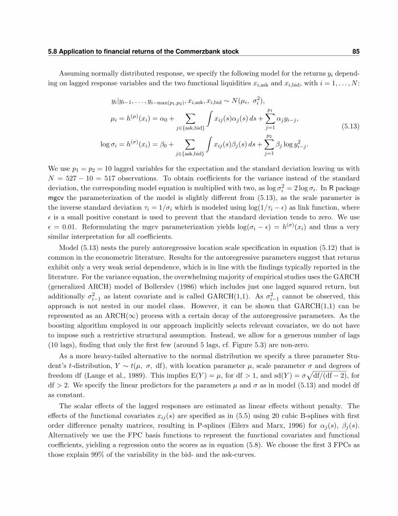
5.8 Application to financial returns of the Commerzbank stock 85
Assuming normally distributed response, we specify the following model for the returns yi depend-
ing on lagged response variables and the two functional liquidities xi,ask and xi,bid, with i = 1, . . . , N :
yi|yi−1, . . . , yi−max(p1,p2), xi,ask, xi,bid ∼ N(µi, σ2i ),
µi = h(µ)(xi) = α0 +∑
j∈{ask,bid}
∫xij(s)αj(s) ds+
p1∑j=1
αjyi−j ,
log σi = h(σ)(xi) = β0 +∑
j∈{ask,bid}
∫xij(s)βj(s) ds+
p2∑j=1
βj log y2i−j .
(5.13)
We use p1 = p2 = 10 lagged variables for the expectation and the standard deviation leaving us with
N = 527 − 10 = 517 observations. To obtain coefficients for the variance instead of the standard
deviation, the corresponding model equation is multiplied with two, as log σ2i = 2 log σi. In R package
mgcv the parameterization of the model is slightly different from (5.13), as the scale parameter is
the inverse standard deviation τi = 1/σi which is modeled using log(1/τi − ε) as link function, where
ε is a small positive constant is used to prevent that the standard deviation tends to zero. We use
ε = 0.01. Reformulating the mgcv parameterization yields log(σi − ε) = h(σ)(xi) and thus a very
similar interpretation for all coefficients.
Model (5.13) nests the purely autoregressive location scale specification in equation (5.12) that is
common in the econometric literature. Results for the autoregressive parameters suggest that returns
exhibit only a very weak serial dependence, which is in line with the findings typically reported in the
literature. For the variance equation, the overwhelming majority of empirical studies uses the GARCH
(generalized ARCH) model of Bollerslev (1986) which includes just one lagged squared return, but
additionally σ2i−1 as latent covariate and is called GARCH(1,1). As σ2
i−1 cannot be observed, this
approach is not nested in our model class. However, it can be shown that GARCH(1,1) can be
represented as an ARCH(∞) process with a certain decay of the autoregressive parameters. As the
boosting algorithm employed in our approach implicitly selects relevant covariates, we do not have
to impose such a restrictive structural assumption. Instead, we allow for a generous number of lags
(10 lags), finding that only the first few (around 5 lags, cf. Figure 5.3) are non-zero.
As a more heavy-tailed alternative to the normal distribution we specify a three parameter Stu-
dent’s t-distribution, Y ∼ t(µ, σ, df), with location parameter µ, scale parameter σ and degrees of
freedom df (Lange et al., 1989). This implies E(Y ) = µ, for df > 1, and sd(Y ) = σ√
df/(df− 2), for
df > 2. We specify the linear predictors for the parameters µ and σ as in model (5.13) and model df
as constant.
The scalar effects of the lagged responses are estimated as linear effects without penalty. The
effects of the functional covariates xij(s) are specified as in (5.5) using 20 cubic B-splines with first
order difference penalty matrices, resulting in P-splines (Eilers and Marx, 1996) for αj(s), βj(s).
Alternatively we use the FPC basis functions to represent the functional covariates and functional
coefficients, yielding a regression onto the scores as in equation (5.8). We choose the first 3 FPCs as
those explain 99% of the variability in the bid- and the ask-curves.
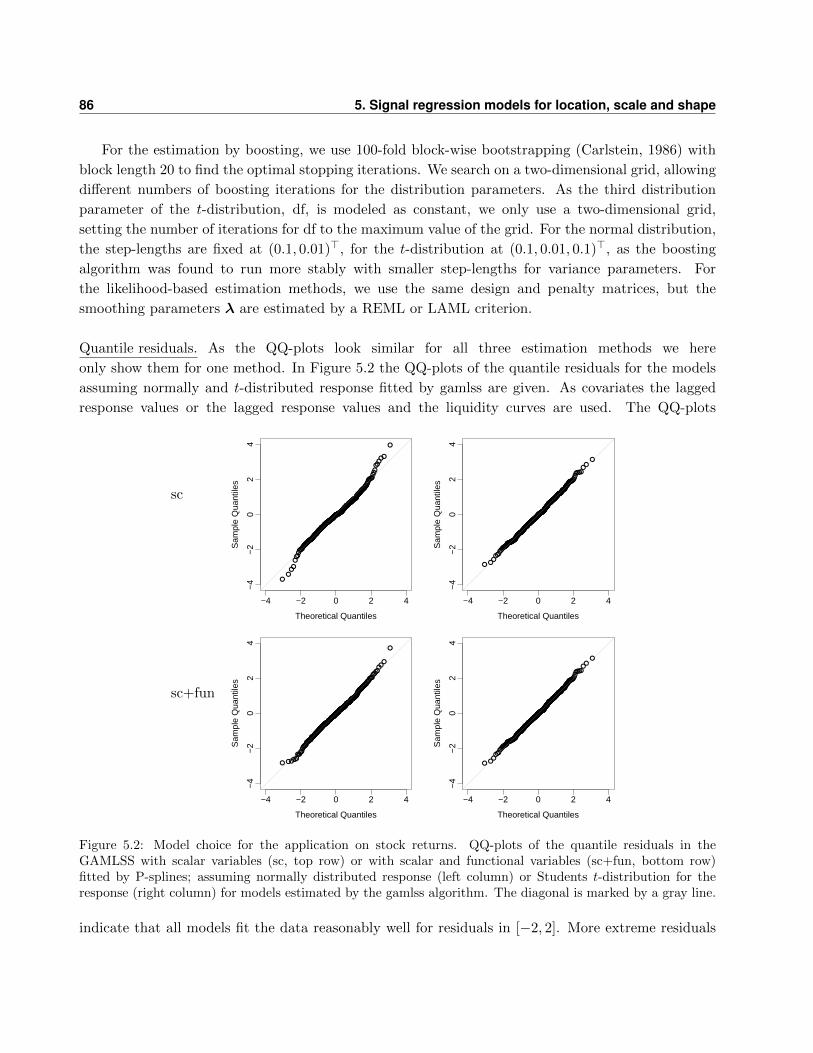
86 5. Signal regression models for location, scale and shape
For the estimation by boosting, we use 100-fold block-wise bootstrapping (Carlstein, 1986) with
block length 20 to find the optimal stopping iterations. We search on a two-dimensional grid, allowing
different numbers of boosting iterations for the distribution parameters. As the third distribution
parameter of the t-distribution, df, is modeled as constant, we only use a two-dimensional grid,
setting the number of iterations for df to the maximum value of the grid. For the normal distribution,
the step-lengths are fixed at (0.1, 0.01)>, for the t-distribution at (0.1, 0.01, 0.1)>, as the boosting
algorithm was found to run more stably with smaller step-lengths for variance parameters. For
the likelihood-based estimation methods, we use the same design and penalty matrices, but the
smoothing parameters λ are estimated by a REML or LAML criterion.
Quantile residuals. As the QQ-plots look similar for all three estimation methods we here
only show them for one method. In Figure 5.2 the QQ-plots of the quantile residuals for the models
assuming normally and t-distributed response fitted by gamlss are given. As covariates the lagged
response values or the lagged response values and the liquidity curves are used. The QQ-plots
sc
●
●
●
●●
●●
●●
●
●
●
●
●
●●
●
●
●
●
●
●
●
●
●
●
●
●
●
●
●
●
●
●●
●
●●
●
●
●
●
●
●
●
●
●
●
●
●●●
●
●
●
●
●
●
●●
●
●
●
●
●
●
●
●
●
●
●
●
●
●
●
●●
●
●
●
●
●
●
●
●
●
●
●
●
●
●
●
●
●●
●
●
●●
●
●
●
●
●
●●
●
●
●
●●
●
●
●●
●
●●
●
●
●
●
●
●
●●
●
●
●
●
●●
●●
●
●
●
●●
●
●
●
●
●●
●
●
●●●●
●
●
●
●
●
●
●●
●
●
●
●
●
●
●
●
●
●
●
●●
●
●
●
●
●●
●●
●●●
●
●
●
●
●
●
●●●
●
●
●
●
●●●
●
●
●●
●
●
●●
●●
●
●
●
●
●
●●
●
●
●
●●●
●
●
●
●
●
●
●
●
●
●
●●
●
●
●●
●
●●
●
●
●
●
●
●
●
●
●
●
●
●
●
●●
●
●
●●
●
●●
●
●●●
●
●
●
●
●●
●
●●
●●
●
●
●
●
●●
●
●
●
●
●
●
●
●●
●
●
●●
●●
●
●●●
●
●●
●●
●●
●●
●
●
●
●
●
●●
●●●●
●
●
●
●
●
●
●●
●
●
●
●
●
●
●
●
●
●●
●
●
●●
●
●
●
●
●
●
●●
●
●
●
●
●
●●
●
●
●
●●
●
●
●●
●
●
●
●
●
●
●
●
●
●
●●
●
●
●●
●
●●
●●
●
●
●
●●
●●
●
●●
●●
●●●
●
●●●
●●
●
●●
●
●
●●
●
●
●
●
●
●
●
●
●
●
●
●●
●●
●
●
●
●●
●●
●
●
●●●
●●
●
●
●●
●
●●
●
●●
●
●
●
●
●●
●
−4 −2 0 2 4
−4
−2
02
4
Theoretical Quantiles
Sam
ple
Qua
ntile
s
●
●
●
●●
●
●
●●
●●
●
●
●●
●
●
●
●
●
●
●
●
●
●
●
●
●
●
●
●
●●
●●●
●●
●
●
●
●
●
●
●
●
●
●
●
●●●
●
●
●
●
●
●
●●
●
●
●
●
●
●
●
●
●
●
●
●
●
●
●
●●
●
●
●
●
●
●
●
●
●
●
●
●
●
●
●
●
●●
●
●
●
●
●
●
●
●
●
●●
●
●
●
●●
●
●
●●
●
●
●●
●
●
●
●
●
●
●
●
●
●
●
●●
●●
●
●
●
●
●
●
●
●
●
●
●
●
●
●
●●●
●
●
●
●●
●
●●
●
●
●
●
●
●
●
●
●
●
●
●●
●
●
●
●
●●
●●
●●●
●
●
●
●
●
●
●●●
●
●
●
●
●●
●
●
●
●●
●
●
●●
●●
●
●
●
●
●
●●
●
●
●
●●
●
●
●
●
●
●
●
●
●
●
●
●
●
●
●
●●
●
●
●●
●
●
●
●
●
●
●
●
●
●
●
●
●●
●
●
●●
●
●
●
●
●●●
●
●
●
●
●●
●
●●
●●
●
●
●
●
●●
●
●
●
●
●
●
●
●●
●
●
●●
●●
●
●●●
●
●●
●●
●●
●
●
●
●
●
●
●
●
●
●
●●●
●
●
●
●
●
●
●●
●
●
●
●
●
●
●
●
●
●●
●
●
●●
●
●
●
●
●
●
●●
●
●
●
●
●
●
●
●
●
●
●●
●
●
●
●
●
●
●
●
●
●
●
●
●
●
●●
●
●
●
●
●
●●
●●
●
●
●
●●
●●
●
●
●
●●
●●●
●
●●●
●●
●
●●
●
●
●●
●
●
●
●
●
●
●
●
●
●
●
●●
●●
●
●
●
●
●
●
●
●
●
●●●
●●
●
●
●
●
●
●●
●
●●
●
●
●
●
●●
●
−4 −2 0 2 4
−4
−2
02
4
Theoretical Quantiles
Sam
ple
Qua
ntile
s
sc+fun
●
●
●●
●
●●●●
●●
●
●
●●●
●
●
●
●
●
●
●
●
●●
●
●
●
●
●
●
●
●●●
●●●
●
●
●
●
●
●
●
●
●●
●●●
●
●
●
●
●
●
●●
●
●
●
●
●
●
●
●
●
●
●
●
●
●
●●
●
●●
●
●
●
●
●
●●
●
●
●
●
●●
●
●●
●
●
●●
●
●
●
●●
●
●
●
●
●
●●
●
●
●●
●
●
●
●
●
●
●
●
●
●●
●
●
●
●
●●
●●
●
●
●
●
●
●
●
●
●
●●
●
●
●●
●
●
●●
●
●●
●
●●●●
●
●
●
●
●
●
●
●
●
●●
●
●
●
●
●
●
●
●
●
●
●
●
●
●
●●
●
●●
●●
●
●
●
●●
●
●
●
●●●
●
●
●
●
●
●
●
●
●
●●●
●
●
●
●
●●
●
●
●
●
●
●
●
●
●
●
●●●
●
●●
●●●●●
●
●
●●
●
●
●
●
●
●
●
●●
●
●
●●
●
●
●
●
●●●
●
●
●
●
●●
●
●
●
●●
●
●
●
●
●●
●
●
●
●
●
●●
●●
●
●
●●
●●
●
●●●
●
●
●
●
●
●
●●
●
●
●
●●
●●
●
●
●
●
●
●
●
●●
●
●
●
●
●
●
●●
●
●
●
●
●
●●
●
●
●
●
●●
●
●
●
●
●
●
●
●●
●
●
●
●
●
●
●
●
●
●
●
●
●
●
●
●
●
●
●
●
●
●
●
●●
●
●
●
●
●
●
●●
●
●
●
●
●
●
●
●
●
●
●
●●
●●●
●
●●
●
●●
●
●●
●
●
●●
●●
●
●
●
●
●
●
●
●
●
●●●●
●
●●
●●
●
●
●
●
●●
●●
●
●●
●●
●
●●
●
●●
●
●
●
●
●●
●
−4 −2 0 2 4
−4
−2
02
4
Theoretical Quantiles
Sam
ple
Qua
ntile
s
●
●
●
●●
●
●
●●
●●
●
●
●●
●
●
●
●
●
●
●
●
●
●
●
●
●
●
●
●
●●
●●●
●●
●
●
●
●
●
●
●
●
●
●
●
●●●
●
●
●
●
●
●
●●
●
●
●
●
●
●
●
●
●
●
●
●
●
●
●
●●
●
●
●
●
●
●
●
●
●
●
●
●
●
●
●
●
●●
●
●
●
●
●
●
●
●
●
●●
●
●
●
●●
●
●
●●
●
●
●●
●
●
●
●
●
●
●
●
●
●
●
●●
●●
●
●
●
●
●
●
●
●
●
●
●
●
●
●
●●●
●
●
●
●●
●
●●
●
●
●
●
●
●
●
●
●
●
●
●●
●
●
●
●
●●
●●
●●●
●
●
●
●
●
●
●●●
●
●
●
●
●●
●
●
●
●●
●
●
●●
●●
●
●
●
●
●
●●
●
●
●
●●
●
●
●
●
●
●
●
●
●
●
●
●
●
●
●
●●
●
●
●●
●
●
●
●
●
●
●
●
●
●
●
●
●●
●
●
●●
●
●
●
●
●●●
●
●
●
●
●●
●
●●
●●
●
●
●
●
●●
●
●
●
●
●
●
●
●●
●
●
●●
●●
●
●●●
●
●●
●●
●●
●
●
●
●
●
●
●
●
●
●
●●●
●
●
●
●
●
●
●●
●
●
●
●
●
●
●
●
●
●●
●
●
●●
●
●
●
●
●
●
●●
●
●
●
●
●
●
●
●
●
●
●●
●
●
●
●
●
●
●
●
●
●
●
●
●
●
●●
●
●
●
●
●
●●
●●
●
●
●
●●
●●
●
●
●
●●
●●●
●
●●●
●●
●
●●
●
●
●●
●
●
●
●
●
●
●
●
●
●
●
●●
●●
●
●
●
●
●
●
●
●
●
●●●
●●
●
●
●
●
●
●●
●
●●
●
●
●
●
●●
●
−4 −2 0 2 4
−4
−2
02
4
Theoretical Quantiles
Sam
ple
Qua
ntile
s
Figure 5.2: Model choice for the application on stock returns. QQ-plots of the quantile residuals in theGAMLSS with scalar variables (sc, top row) or with scalar and functional variables (sc+fun, bottom row)fitted by P-splines; assuming normally distributed response (left column) or Students t-distribution for theresponse (right column) for models estimated by the gamlss algorithm. The diagonal is marked by a gray line.
indicate that all models fit the data reasonably well for residuals in [−2, 2]. More extreme residuals
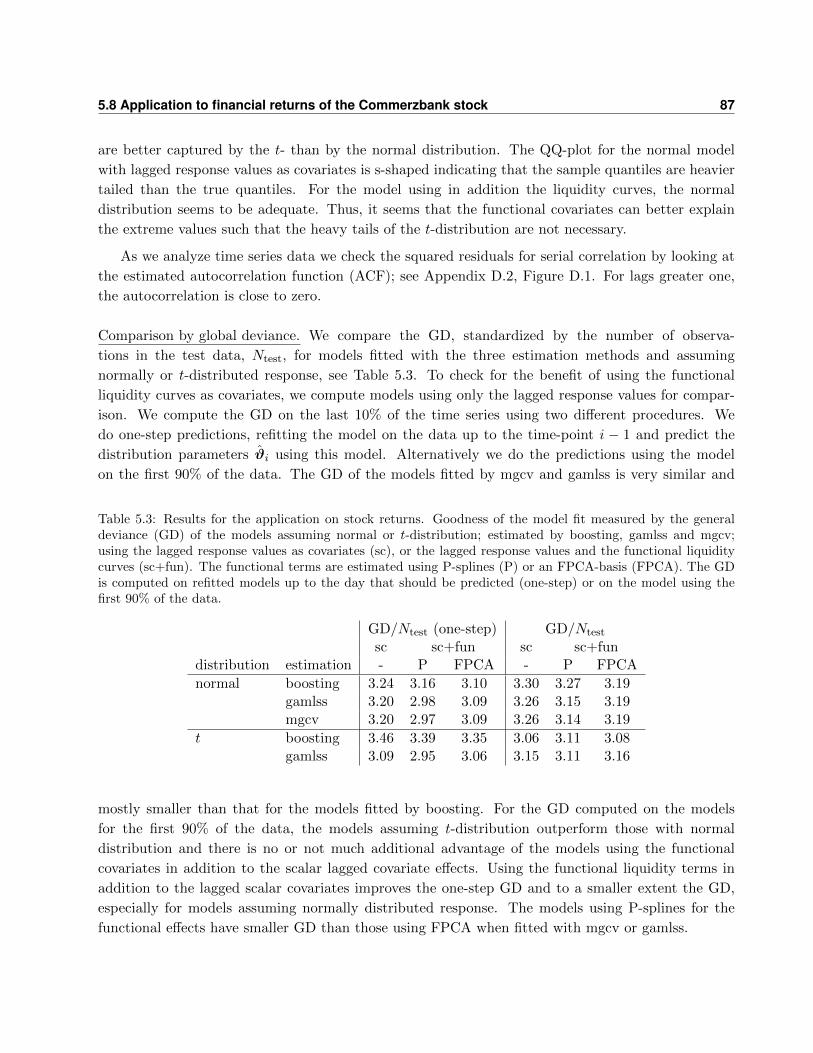
5.8 Application to financial returns of the Commerzbank stock 87
are better captured by the t- than by the normal distribution. The QQ-plot for the normal model
with lagged response values as covariates is s-shaped indicating that the sample quantiles are heavier
tailed than the true quantiles. For the model using in addition the liquidity curves, the normal
distribution seems to be adequate. Thus, it seems that the functional covariates can better explain
the extreme values such that the heavy tails of the t-distribution are not necessary.
As we analyze time series data we check the squared residuals for serial correlation by looking at
the estimated autocorrelation function (ACF); see Appendix D.2, Figure D.1. For lags greater one,
the autocorrelation is close to zero.
Comparison by global deviance. We compare the GD, standardized by the number of observa-
tions in the test data, Ntest, for models fitted with the three estimation methods and assuming
normally or t-distributed response, see Table 5.3. To check for the benefit of using the functional
liquidity curves as covariates, we compute models using only the lagged response values for compar-
ison. We compute the GD on the last 10% of the time series using two different procedures. We
do one-step predictions, refitting the model on the data up to the time-point i − 1 and predict the
distribution parameters ϑi using this model. Alternatively we do the predictions using the model
on the first 90% of the data. The GD of the models fitted by mgcv and gamlss is very similar and
Table 5.3: Results for the application on stock returns. Goodness of the model fit measured by the generaldeviance (GD) of the models assuming normal or t-distribution; estimated by boosting, gamlss and mgcv;using the lagged response values as covariates (sc), or the lagged response values and the functional liquiditycurves (sc+fun). The functional terms are estimated using P-splines (P) or an FPCA-basis (FPCA). The GDis computed on refitted models up to the day that should be predicted (one-step) or on the model using thefirst 90% of the data.
GD/Ntest (one-step) GD/Ntest
sc sc+fun sc sc+fundistribution estimation - P FPCA - P FPCA
normal boosting 3.24 3.16 3.10 3.30 3.27 3.19gamlss 3.20 2.98 3.09 3.26 3.15 3.19mgcv 3.20 2.97 3.09 3.26 3.14 3.19
t boosting 3.46 3.39 3.35 3.06 3.11 3.08gamlss 3.09 2.95 3.06 3.15 3.11 3.16
mostly smaller than that for the models fitted by boosting. For the GD computed on the models
for the first 90% of the data, the models assuming t-distribution outperform those with normal
distribution and there is no or not much additional advantage of the models using the functional
covariates in addition to the scalar lagged covariate effects. Using the functional liquidity terms in
addition to the lagged scalar covariates improves the one-step GD and to a smaller extent the GD,
especially for models assuming normally distributed response. The models using P-splines for the
functional effects have smaller GD than those using FPCA when fitted with mgcv or gamlss.
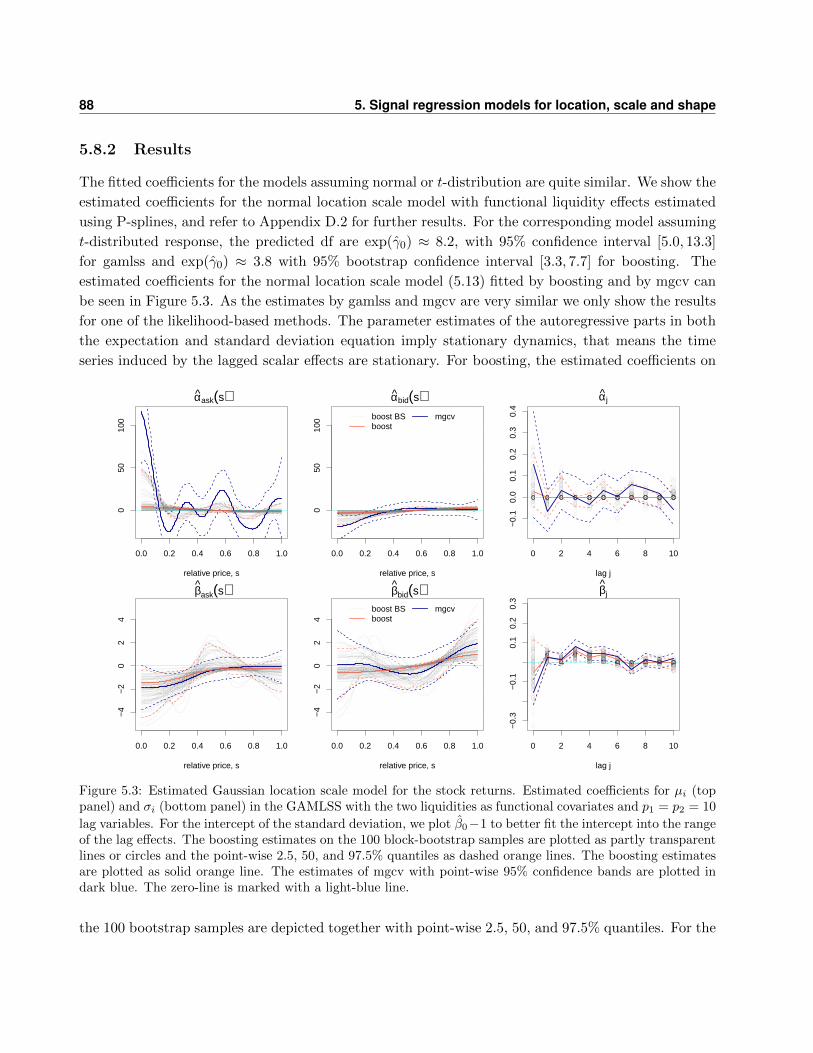
88 5. Signal regression models for location, scale and shape
5.8.2 Results
The fitted coefficients for the models assuming normal or t-distribution are quite similar. We show the
estimated coefficients for the normal location scale model with functional liquidity effects estimated
using P-splines, and refer to Appendix D.2 for further results. For the corresponding model assuming
t-distributed response, the predicted df are exp(γ0) ≈ 8.2, with 95% confidence interval [5.0, 13.3]
for gamlss and exp(γ0) ≈ 3.8 with 95% bootstrap confidence interval [3.3, 7.7] for boosting. The
estimated coefficients for the normal location scale model (5.13) fitted by boosting and by mgcv can
be seen in Figure 5.3. As the estimates by gamlss and mgcv are very similar we only show the results
for one of the likelihood-based methods. The parameter estimates of the autoregressive parts in both
the expectation and standard deviation equation imply stationary dynamics, that means the time
series induced by the lagged scalar effects are stationary. For boosting, the estimated coefficients on
0.0 0.2 0.4 0.6 0.8 1.0
050
100
αask(s)
relative price, s
0.0 0.2 0.4 0.6 0.8 1.0
050
100
αbid(s)
relative price, s
boost BSboost
mgcv
0 2 4 6 8 10
−0.
10.
00.
10.
20.
30.
4
αj
lag j
0.0 0.2 0.4 0.6 0.8 1.0
−4
−2
02
4
βask(s)
relative price, s
0.0 0.2 0.4 0.6 0.8 1.0
−4
−2
02
4
βbid(s)
relative price, s
boost BSboost
mgcv
0 2 4 6 8 10
−0.
3−
0.1
0.1
0.2
0.3
βj
lag j
Figure 5.3: Estimated Gaussian location scale model for the stock returns. Estimated coefficients for µi (toppanel) and σi (bottom panel) in the GAMLSS with the two liquidities as functional covariates and p1 = p2 = 10
lag variables. For the intercept of the standard deviation, we plot β0−1 to better fit the intercept into the rangeof the lag effects. The boosting estimates on the 100 block-bootstrap samples are plotted as partly transparentlines or circles and the point-wise 2.5, 50, and 97.5% quantiles as dashed orange lines. The boosting estimatesare plotted as solid orange line. The estimates of mgcv with point-wise 95% confidence bands are plotted indark blue. The zero-line is marked with a light-blue line.
the 100 bootstrap samples are depicted together with point-wise 2.5, 50, and 97.5% quantiles. For the

5.9 Simulation studies 89
mgcv-approach, the estimated coefficient functions are given with point-wise 95% confidence intervals.
The estimated coefficients for the standard deviation are quite similar. Regarding the effects on the
expectation, the size and smoothness of the estimated coefficients obtained by mgcv and by boosting
differs considerably, as the coefficients obtained by boosting are shrunken towards zero.
In a simulation study, see Section 5.9 and Appendix D.3, we observe that depending on how much
information the functional covariates contain, the functional coefficients can be estimated with more
or less accuracy. The functional covariates in this application contain relatively little information
as in an FPCA more than 99% of the variance can be explained by the first three FPCs and the
explained variance per principal component is strongly decreasing.
When using only a small number of basis functions in the specification of the functional effects
in mgcv (e.g., Kj = 10 instead of 20) and using the shrinkage penalty of Marra and Wood (2011),
mgcv yields similar estimates like boosting (with Kj = 10 or 20); see Figure D.2 in Appendix D.2.
When the number of boosting iterations is increased, the boosting-estimates become similar to those
obtained by mgcv (not shown). Thus, the different results are mainly due to the different selection
and estimation of hyper-parameters that imply different choices for the effective degrees of freedom
for the smooth effects.
The effect size depends on the underlying modeling assumptions and we will only interpret the
direction of the effects (positive or negative), as those are estimated stably. These directions of the
effects remain, even when fitting the models using FPCA-basis functions, although the shape of the
functional effects changes, as the effects are assumed to lie in the space spanned by the FPCA-
basis functions. This implies for this application that all functional effects start almost in zero
(cf. Figure D.3).
Looking at the estimated functional coefficients in Figure 5.3, the absolute values of the estimated
coefficient functions are generally higher for small s, which is sensible, as the bid and ask curves for
small s describe the liquidity close to the mid-price. For the effects on the expectation, the estimates
of αask(s) are positive and αbid(s) are negative near the mid-price. Thus, higher liquidity of the ask
side and lower liquidity of the bid side tend to be associated with an increase of the expected returns.
The lagged response values seem to have no influence on the expectation, as αj is virtually always
zero for the boosting estimation, and close to zero for the mgcv-estimation with confidence bands
containing zero. Looking at the model for the standard deviation, the estimated coefficient functions
for ask, βask(s), are mostly negative. This means that higher liquidity leads to lower variances, and
lower liquidity leads to higher variances. The estimated coefficients for the bid curves, βbid(s), are
quite close to zero. The lagged squared response values seem to have an influence for close time-points,
as many βj are greater zero for the first five lags.
5.9 Simulation studies
In the following, we present a simulation study using the observed functional covariates of the appli-
cation and coefficient functions resembling the estimated ones. Then we comment on the results of a
more general simulation study comparing the estimation methods systematically in different settings.
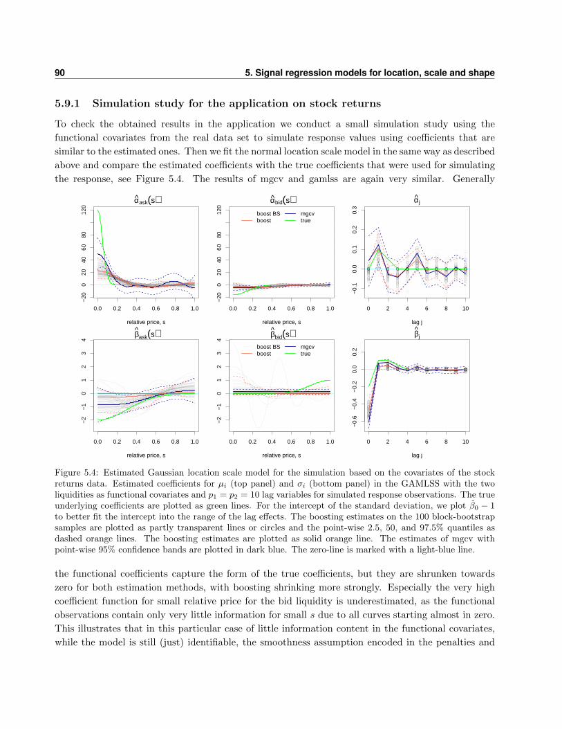
90 5. Signal regression models for location, scale and shape
5.9.1 Simulation study for the application on stock returns
To check the obtained results in the application we conduct a small simulation study using the
functional covariates from the real data set to simulate response values using coefficients that are
similar to the estimated ones. Then we fit the normal location scale model in the same way as described
above and compare the estimated coefficients with the true coefficients that were used for simulating
the response, see Figure 5.4. The results of mgcv and gamlss are again very similar. Generally
0.0 0.2 0.4 0.6 0.8 1.0
−20
020
4060
8012
0
αask(s)
relative price, s
0.0 0.2 0.4 0.6 0.8 1.0
−20
020
4060
8012
0
αbid(s)
relative price, s
boost BSboost
mgcvtrue
0 2 4 6 8 10
−0.
10.
00.
10.
20.
3
αj
lag j
0.0 0.2 0.4 0.6 0.8 1.0
−2
−1
01
23
4
βask(s)
relative price, s
0.0 0.2 0.4 0.6 0.8 1.0
−2
−1
01
23
4
βbid(s)
relative price, s
boost BSboost
mgcvtrue
0 2 4 6 8 10
−0.
6−
0.4
−0.
20.
00.
2
βj
lag j
Figure 5.4: Estimated Gaussian location scale model for the simulation based on the covariates of the stockreturns data. Estimated coefficients for µi (top panel) and σi (bottom panel) in the GAMLSS with the twoliquidities as functional covariates and p1 = p2 = 10 lag variables for simulated response observations. The trueunderlying coefficients are plotted as green lines. For the intercept of the standard deviation, we plot β0 − 1to better fit the intercept into the range of the lag effects. The boosting estimates on the 100 block-bootstrapsamples are plotted as partly transparent lines or circles and the point-wise 2.5, 50, and 97.5% quantiles asdashed orange lines. The boosting estimates are plotted as solid orange line. The estimates of mgcv withpoint-wise 95% confidence bands are plotted in dark blue. The zero-line is marked with a light-blue line.
the functional coefficients capture the form of the true coefficients, but they are shrunken towards
zero for both estimation methods, with boosting shrinking more strongly. Especially the very high
coefficient function for small relative price for the bid liquidity is underestimated, as the functional
observations contain only very little information for small s due to all curves starting almost in zero.
This illustrates that in this particular case of little information content in the functional covariates,
while the model is still (just) identifiable, the smoothness assumption encoded in the penalties and

5.10 Discussion 91
the early stopping, which leads to a shrinkage effect, still strongly influences the estimates. The
strength of this effect differs between the two estimation approaches, but is in the same direction.
For our application, this implies that the true effects might be underestimated, but that the sign of
the effects should be interpretable as we assumed.
5.9.2 General simulation study
The aim of the simulation study is to check and compare the model fits of the different implementa-
tions systematically. Mayr et al. (2012) conduct a simulation study for boosting GAMLSS with scalar
covariates. In Wood et al. (2015) the performance of mgcv and gamlss is compared for some settings
with scalar covariates. We thus focus on the estimation of effects of functional covariates. For the
generation of functional covariates, we use different processes resulting in functional covariates con-
taining different amounts of information. Comparing the estimates of the functional effects over those
settings shows that the data generating process of the functional covariates strongly influences the
estimation accuracy of the functional effects. This has already been discussed in Scheipl and Greven
(2016) for mean models. On the other hand we vary the complexity of the functional coefficients from
zero-coefficients over almost linear to u-shaped coefficient functions and functions with a steep bend.
With growing complexity of the coefficient functions the estimates tend to get worse. Generally one
can observe in the normal location scale model that the coefficient estimates for the expectation are
better than those for the standard deviation.
In the simulation study the most difficult data setting, i.e. the one with the least information
in the covariates, best reflects the data situation in the application on stock returns. In this case
the coefficient estimates often underestimate the absolute value of the coefficients. For less patho-
logical data situations, the estimates are usually close to the true functions and all three estimation
approaches yield very similar estimates and predictions. See Appendix D.3 for details on the data
generation and the results of this simulation study.
5.10 Discussion
In this chapter, we discuss the extension of scalar-on-function regression to GAMLSS. The flexibility
of the approach allows to model many different response distributions with parameter-specific lin-
ear predictors, containing effects of functional and scalar covariates. The two proposed estimation
methods based on boosting and on penalized likelihood are beneficial in different data settings. The
component-wise gradient boosting algorithm can be used in high-dimensional data settings and for
large data sets. The likelihood-based methods provide inference based on mixed models and can be
computed faster for small data sets.
We believe that the combination of scalar-on-function regression and GAMLSS is an important
extension to functional regression models with many possible applications in different fields. In par-
ticular, scalar-on-function models for zero-inflated or over-dispersed count data as well as bounded
continuous response distributions can be fitted within the GAMLSS framework. In contrast to quan-

92 5. Signal regression models for location, scale and shape
tile regression models with functional covariates (e.g., Ferraty et al., 2005; Cardot et al., 2005; Chen
and Muller, 2012a) GAMLSS provide coherent interpretable models for all distribution parameters,
prevent quantile crossing and allow for simultaneous inference at the price of assuming a particular
response distribution.
In future research, we will consider GAMLSS for functional responses with scalar and/or functional
covariates, with the aim of extending the flexible functional additive mixed model framework of Scheipl
et al. (2015) and Chapters 3 and 4, estimated by penalized likelihood and boosting, respectively, to
simultaneous models for several response distribution parameters.
Acknowledgments
The authors thank Deutsche Borse AG for providing the XETRA historical limit order book data as
part of a cooperation with the Chair of Financial Econometrics, LMU Munich, Germany. The work
of Sarah Brockhaus and Sonja Greven was supported by the German Research Foundation through
Emmy Noether grant GR 3793/1-1.

Chapter 6
On the practical use of the R package
FDboost
Software
For this chapter, the analyses were conducted in R version 3.2.3 (R Core Team, 2015). We used
FDboost 0.2-0 (Brockhaus and Rugamer, 2016), mboost 2.6-0 (Hothorn et al., 2016) and gamboostLSS
1.2-1 (Hofner et al., 2015b). The Canadian weather data were taken from R package fda 2.4.4 (Ramsay
et al., 2014).
6.1 Introduction
The aim of functional data analysis (FDA) is to analyze data that has a functional nature. The
field was popularized by Ramsay and Silverman (2005). Due to technical advances more and more
functional data are observed. Such data can be found in many scientific fields like demography, biology,
medicine, meteorology and economics (see, e.g., Ullah and Finch, 2013). We deal with functional data
that are curves observed over an interval on R. Examples for such data are growth curves over time
or spectrometric measurements over a spectrum of wavelengths. Regression models are a versatile
tool for data analysis and various models have been proposed for regression with functional variables;
see Morris (2015) for a recent review of functional regression models. One can distinguish between
three different types of functional regression models depending on where functional variables enter the
model: scalar-on-function regression means regression with scalar response and functional covariates;
function-on-scalar regression denotes models with functional response and scalar covariates; and the
term function-on-function regression is used when both response and covariates are functional. We
propose a generic framework for regression with functional response and/or functional covariates
(see Chapters 2, 3 and 4). In this framework, many types of covariate effects are possible including
linear and non-linear effects of scalar covariates as well as linear effects of functional covariates and
interaction effects. Furthermore, it is possible to combine all those effects within one model. The
modeled feature of the conditional response distribution can be chosen flexibly. The framework
94 6. On the practical use of the R package FDboost
includes linear models (LMs), generalized linear models (GLMs), as well as quantile and expectile
regression. Furthermore, generalized additive models for location, scale and shape (GAMLSS, Rigby
and Stasinopoulos, 2005) can be fitted. GAMLSS can model all distribution parameters of the
conditional response distribution simultaneously depending on covariates. In Chapter 5 we discuss
GAMLSS with scalar response and functional covariates.
For fitting, a suitable loss function whose population minimizer corresponds to the modeled charac-
teristic of the response is defined and optimized. For mean regression, for instance, the corresponding
loss is the squared error loss. We conduct the fitting by a component-wise gradient boosting algo-
rithm (Buhlmann and Hothorn, 2007). Boosting improves the model fit by iteratively combining
simple models and can be seen as a method for gradient descent. Boosting can estimate models in
high-dimensional data settings and inherently does variable selection.
Flexible regression models for functional response have been proposed in a mixed models frame-
work (Ivanescu et al., 2015; Scheipl et al., 2016) and in a Bayesian context (Meyer et al., 2015). They
allow for a variety of covariate effects including functional terms. But for the modeled feature of the
conditional response distribution, they are restricted to mean regression.
In this chapter, we present the R package FDboost, which is designed to fit a great variety of func-
tional regression models by boosting. FDboost builds on the mboost package for statistical boosting.
Thus, in the back-end we rely on a well-tested and efficient implementation. FDboost provides a com-
prehensive implementation of the most important methods for boosting functional regression models.
In particular, this package makes it possible to conveniently fit models with functional response. Var-
ious base-learners that model effects of functional covariates are implemented. Furthermore, FDboost
contains functions for tuning models and displaying results, which are suited to regression with func-
tional variables. We illustrate the practical use of FDboost by fitting various models to the Canadian
weather data (Ramsay and Silverman, 2005). As the data are publicly available in the R package fda
the analyses are fully reproducible.
The remainder of the chapter is structured as follows: We shortly review the generic functional
regression model (Section 6.2) and the boosting algorithm that is used for model fitting (Section 6.3).
Then, we introduce the Canadian weather data, which we use as case study throughout this chapter
(Section 6.4). In Section 6.5, we give details on the infrastructure of FDboost. We discuss the model
setup including the modeled characteristic of the response distribution and possible covariate effects.
Then we give details on model tuning and how to extract and display the results. The chapter
concludes with a discussion in Section 6.6.
6.2 The generic functional regression model
First, we introduce some notation. We denote the functional response by Y (t), where t is the eval-
uation point at which the function is observed. We assume that t ∈ T , where T is a real-valued
interval [T1, T2]. For scalar response, we set T1 = T2, such that we only have one single observation
point. The covariate set X can contain both scalar and functional variables. We denote scalar co-
variates by Z and functional covariates by X(s), with s ∈ S = [S1, S2] and S1, S2 ∈ R. We assume
6.2 The generic functional regression model 95
to observe data (yi(t), xi), for i = 1, . . . , N cases. The response can be observed on one common
grid or on curve-specific grids. For responses observed on one common grid, we write yi(tg), with
tg ∈ (t1, . . . , tG)>. For curve-specific evaluation points, the observations are denoted by yi(tig), with
tig ∈ (ti1, . . . , tiGi)>.
For functional response Y (t) and covariates X, the generic model defined in (2.1) can be written
explicitly as a function of t:
ξ(Y |X = x)(t) = h(x)(t) =J∑j=1
hj(x)(t), (6.1)
where ξ is the transformation function, h(x)(t) is the linear predictor and hj(x)(t) are the covariate
effects. The transformation function determines which characteristic of the response distribution is
modeled. It can be, for instance, the expectation, the median or a quantile. The transformation
function can be a composed function, e.g., composing the expectation with a link function to form a
GLM. Each effect hj(x)(t) can depend on one or several covariates in x. Possible effects include linear
and non-linear effects of scalar covariates as well as linear effects of functional covariates. Moreover,
group-specific effects and interaction effects between scalar and functional variables are possible. The
effects hj(x)(t) are linearized by using a basis representation:
hj(x)(t) = bjY (x, t)>θj , j = 1, . . . , J, (6.2)
where the basis bjY (x, t) ∈ RKjY depends on covariates x and the observation-point of the response t.
θj ∈ RKjY is the corresponding coefficient vector that has to be estimated. We represent effect (6.2)
by the row tensor product � of two marginal bases (Scheipl et al., 2015, Chapter 4):
hj(xi)(tig) =(bj(xi, tig)
> � bY (tig)>)θj , (6.3)
where bj(xi, tig) ∈ RKj and bY (tig) ∈ RKY , such that KjY = KjKY . For many covariate effects, the
first basis simplifies to bj(xi) as it only depends on xi and not on tig. If the first basis only depends on
the covariates xi and the second basis only depends on the observation point tg, we use the following
representation (Chapter 3)
hj(xi)(ti) =(bj(xi)
> ⊗ bY (tg)>)θj , (6.4)
that computes the design matrix as the Kronecker product ⊗ of the two marginal bases. Note that
this representation is only possible for responses observed on one common grid, as otherwise bY (tg)
depends on the curve-specific grid points tig. If the effect can be represented as in (6.4) it fits into
the framework of linear array models (Currie et al., 2006). The representation as an array model has
computational advantages as it saves time and memory. In Chapter 3 array models are discussed in
the context of functional regression. For more details on the representation of effects as a row tensor
product basis and as a Kronecker product basis, we refer to Section 2.2.

96 6. On the practical use of the R package FDboost
The effects (6.3) and (6.4) are regularized by a Ridge-type penalty term θ>j P jY θj . The penalty
matrix can be constructed as (Wood, 2006, Sec. 4.1.8)
P jY = λj(P j ⊗ IKY) + λY (IKj ⊗ P Y ), (6.5)
where P j is a suitable penalty for bj and P Y is a suitable penalty for bY . The non-negative smoothing
parameters λj and λY determine the degree of smoothing in each direction. The anisotropic penalty
in (6.5) can be simplified to an isotropic penalty depending on only one smoothing parameter λj ≥ 0:
P jY = λj(P j ⊗ IKY+ IKj ⊗ P Y ). (6.6)
In this simplified penalty only one instead of two smoothing parameters has to be estimated. If the
marginal penalty P j = 0 in penalty (6.6) one gets a penalty that only penalizes the marginal basis
in t direction:
P jY = λj(IKj ⊗ P Y ). (6.7)
6.3 Gradient boosting
Boosting originates in machine learning and aims at combining many weak learners to form a single
strong learner for classification (e.g., Friedman et al., 2000; Schapire and Freund, 2012). Weak learners
are only weakly correlated to the response and thus only slightly better than random guessing. A
strong learner, on the other hand, is highly correlated with the response and predicts very well. In
the boosting context, the weak learners are called base-learners. Boosting was originally designed for
binary classification problems as was extended in various directions (Mayr et al., 2014b). Nowadays
it is also used to estimate statistical models (Mayr et al., 2014a). Gradient boosting minimizes the
expected loss via steepest gradient descent in a step-wise procedure. In each boosting step, each
base-learner is fitted separately to the negative gradient and only the best fitting base-learner is
selected for the model update; hence the term ’component-wise’. For the selected base-learner, only
a small proportion of the fit is added to the current linear predictor. This proportion is controlled
by the step-length ν. A typical choice is ν = 0.1 (e.g., Buhlmann and Hothorn, 2007). Usually the
algorithm is stopped before convergence. Stopping early leads to regularized effect estimates and
variable selection as base-learners that are never chosen for the update are excluded from the model.
Furthermore, the regularization leads to more stable predictions. The optimal stopping iteration
can be determined by resampling methods like cross-validation, sub-sampling or bootstrapping. For
each fold, the empirical out-of-bag risk is computed and the stopping iteration that yields the lowest
empirical risk is chosen. As resampling must be conducted on the level of independent observations,
the resampling must be done on the level of curves for functional response.
In order to obtain a fair selection of base-learners, the same degrees of freedom (df) should be
specified for each base-learner. It is recommended to use a rather small number of df for all base-
learners to work with weak learners (Kneib et al., 2009; Hofner et al., 2011). The number of df that

6.4 Case study: Canadian weather data 97
can be specified for a base-learner are bounded: the maximal number of df is the number of columns
of the design matrix. For rank-deficient penalties, the minimal possible number of df is the rank of
the null space of the penalty. Consider P-splines (Eilers and Marx, 1996) as an example. For dth
order difference penalty, the (d − 1)th order polynomial remains without penalization. Thus, for a
P-spline base-learner with dth order difference penalty, the minimal possible df is d− 1.
To adapt boosting to functional response, we compute the loss at each point t and integrate
it over the domain of the response T (Chapter 3). To obtain identifiable models, it is necessary
to implement base-learners with identifiability constraints that are suited for functional response.
Furthermore, base-learners to model the effects of functional covariates are needed.
6.4 Case study: Canadian weather data
We use the Canadian weather data (Ramsay and Silverman, 2005), which are publicly available in the
R package fda. The data contain the precipitation and temperature curves for 35 Canadian weather
stations averaged per day for the years 1960 to 1994. As the data is averaged over the course of several
years, we model cyclic effects over the course of the year that assume smoothness between January
1 and December 31. We will use the common logarithm of the precipitation as response variable.
As potential covariates, we consider the averaged yearly precipitation curves and the climatic zones
(factor with four categories: Arctic, Atlantic, Continental and Pacific). In Chapter 3.6.3, we use the
Canadian weather data on a monthly instead of daily basis.
Case study: Canadian weather data
We load the dataset into the working directory and create a list that contains all data that we needfor the model fit: the average daily log-precipitation and the average daily temperature at the 35weather stations (35 × 365 matrices); the mean yearly log-precipitation, the region and the placeof each weather station (vectors of length 35); the time-variable giving the evaluation points of thefunctional response (day, vector of length 365) and the variable giving the evaluation points of thefunctional covariate temperature (day s, vector of length 365). We center the functional covariate’temperature’ at each evaluation point. That means we center the temperature per day.
## load the data
data("CanadianWeather", package = "fda")
## use the data on a daily basis
canada <- with(CanadianWeather,
list(temp = t(dailyAv[ , , "Temperature.C"]), ## temperature
l10precip = t(dailyAv[ , , "log10precip"]), ## log-precipitation
## mean yearly log-precipitation
l10precip_mean = log10(colMeans(dailyAv[ , , "Precipitation.mm"])),
region = factor(region),
place = factor(place),
day = 1:365, ## corresponds to t

98 6. On the practical use of the R package FDboost
day_s = 1:365)) ## corresponds to s
## center the temperature curves per day
canada$tempRaw <- canada$temp
canada$temp <- scale(canada$temp, scale = FALSE)
rownames(canada$temp) <- NULL ## delete the row names
For a descriptive plot of the data on a monthly basis, see Figure 3.7. �
The case study is continued (ctd.) during this chapter to illustrate model fitting, parameter
tuning and display of results using the package FDboost. The end of a paragraph that is part of the
case study is marked by a black diamond �.
6.5 The package FDboost
Fitting functional regression models via boosting is implemented in the R package FDboost. The pack-age uses the fitting algorithm and other infrastructure from the R package mboost. All base-learnersand distribution families that are implemented in mboost can be used within FDboost. Furthermore,many naming conventions and methods in FDboost are implemented in analogy to mboost. Thus,we recommend users of FDboost to first familiarize themselves with mboost. A tutorial for mboostcan be found in Hofner et al. (2014). The main fitting function to estimate models (6.1) is calledFDboost(). The interface of FDboost() is as follows:1
FDboost(formula, timeformula, id = NULL,
numInt = "equal", data, offset = NULL, ...)
The set-up of the covariate effects follows (6.3) and (6.4) by separating the effects into two marginal
parts. The marginal effects bj , j = 1, . . . , J , are represented in the formula as y ∼ base-learner 1 +
base-learner 2 + . . . + base-learner J . The marginal effect bY is represented in the timeformula,
which has the form ∼ base-learner for t. Internally, the base-learners specified in formula are
combined with the base-learner specified in timeformula. When it is possible, the representation
using the Kronecker product (6.4) of the two marginal effects is used. Otherwise, the row tensor
product (6.3) representation is used. The penalty matrix is constructed as in 6.6. Per default, the
response is expected to be a matrix. In this case id = NULL. For a response observed on curve-specific
grids, id specifies for each observed value to which curve it belongs; see Section 6.5.1 below for details.
The data is provided in the data argument as a data.frame or a list. The object specified in data has
to contain the response, its evaluation points and all covariates. The functional covariates must be
represented as <number of curves> by <number of evaluation points> matrices and their evaluation
points have to be part of the data object. Via argument numInt, the numerical integration scheme
for computing the integral over the loss is provided. Per default, numInt = "equal", and thus all
1Note that for the presentation of functions we restrict ourselves to the most important function arguments. For thefull list of arguments, we refer to the corresponding manuals.

6.5 The package FDboost 99
integration weights are set to one; for numInt = "Riemann" Riemann sums are used. Per default a
smooth offset varying over t is computed prior to the model fit. For offset = "scalar", a scalar
offset is computed. This corresponds to one global offset for all t. For more details and the full list
of arguments, see the manual of FDboost().
In the dots-argument ’...’, further arguments passed to mboost() and mboost fit() can be speci-
fied; see the manual of mboost() for details. An important argument is family which determines the
loss- and link-function for the model that is to be fitted. The default is family = Gaussian(), which
corresponds to mean regression. Thus, the squared error loss is optimized and as link function the
identity is used. Via the argument control the number of boosting iterations and the step-length ν
of the boosting algorithm can be specified.
6.5.1 Specification of functional and scalar response
If a functional variable is observed on one common grid, its observations can be represented by a
matrix. In FDboost, such functional variables have to be supplied as <number of curves> by <number
of evaluation points> matrices. That is, a functional response yi(tg), with i = 1, . . . , N curves and
g = 1, . . . , G evaluation points, is stored in a N ×G matrix with cases in rows and evaluation points
in columns. This corresponds to a data representation in wide format. The t variable must be given
as vector (t1, . . . , tG)>.
For the functional response, curve-specific observation grids are possible; that means that the
ith response curve is observed at evaluation points (tig, . . . , tiGi) that are specific for curve i. In
this case, the response is supplied as the vector (y1(t11), . . . , yN (tNGN))>. This vector has length
n =∑N
i=1Gi. The t variable contains all evaluation points (t11, . . . , tNGN)>. The argument id
contains the information which observation belongs to which response curve by a vector (1, . . . , N)>.
The argument id must be supplied as a left-sided formula id = ∼ idvariable. For responses observed
on curve-specific grids, three pieces of information must be supplied: the values of the response, the
evaluation points and the number of the curve to which the observation belongs. This corresponds
to a data representation in long format.
A scalar response is supplied as vector (y1, . . . , yN ). The timeformula, which is used to expand
the effects along the domain of the response, is set to NULL for scalar response.
Case study (ctd.): Canadian weather data
In the following, we give an example for a model fit with the response in wide format and withresponse in long format. We fit an intercept model by a formula y ∼ 1 and a timeformula of theform ∼ bbs(t). As the precipitation is averaged over several years, the precipitation is expected tobe similar for January 1 and December 31. We thus fit a cyclic effect over t.
library(FDboost) ## load package
## fit intercept model with response matrix, i.e. response observed on a common grid
m0 <- FDboost(l10precip ~ 1,

100 6. On the practical use of the R package FDboost
timeformula = ~ bbs(day, cyclic = TRUE, boundary.knots = c(0.5, 365.5)),
offset = "scalar", data = canada)
To fit a model with response in long format, we first have to bring the data into the correspondingformat. The dataset canada l contains the response in long format. In the dataset canada i, 30% ofthe observations are set to missing inducing curve-specific grids of evaluation points.
## response in long-format with potentially curve-specific grids
canada_l <- canada
canada_l$l10precip <- as.vector(t(canada$l10precip)) ## long vector for response
canada_l$id <- rep(1:35, each = 365) ## number of curve i
canada_l$day <- rep(1:365, times = 35) ## evaluation points t
## induce missing values such that the response is observed on curve-specific grids
set.seed(123)
n <- length(canada_l$day)
missing <- sample(1:n, size = 0.3 * n) ## 30% missing
canada_i <- canada_l
canada_i$l10precip <- canada_l$l10precip[!1:n %in% missing]
canada_i$id <- canada_l$id[! 1:n %in% missing]
canada_i$day <- canada_l$day[! 1:n %in% missing]
## fit intercept model for response in long format
m0_l <- FDboost(l10precip ~ 1,
timeformula = ~ bbs(day, cyclic = TRUE, boundary.knots = c(0.5, 365.5)),
id = ~ id, offset = "scalar", data = canada_l) ## or use canada_i
As scalar response, we use the logarithm of the mean annual precipitation.
## fit intercept model for scalar response
m0 <- FDboost(l10precip_mean ~ 1, timeformula = NULL, offset = "scalar", data = canada)
For scalar response, the pure intercept model corresponds to computing the mean of the response. �
6.5.2 Potential covariate effects: base-learners
The effects in covariate direction are specified in the formula argument. The effect in t direction is
specified in timeformula. FDboost() combines the base-learners specified in formula with the base-
learner specified in timeformula. The effects are represented as Kronecker product of two marginal
bases, see Chapter 3, or as row tensor product, see Scheipl et al. (2015) and Chapter 4. For a
detailed comparison between the row tensor and the Kronecker product representation, we refer to
Chapter 2. However, for the practical use of FDboost(), the user does not need to worry whether the
effect is computed as row tensor product or as Kronecker product of two marginal bases, as FDboost()
automatically uses the appropriate operator.
6.5 The package FDboost 101
Effects in the formula that are combined with the timeformula
Many covariate effects can be separated into two marginal bases, such that the first basis only depends
on covariates and the second basis only depends on t. In the array framework, see (6.4), all effects are
represented as Kronecker product of two marginal bases. The bases in covariate direction bj(x) are
specified in formula. The effect in t is specified in timeformula. For array models, FDboost() connects
the effects of formula and timeformula by the operator %O%, yielding base-learner 1 %O% base-learner
t + . . . + base-learner J %O% base-learner t. The operator %O% uses the array framework (Currie
et al., 2006) to efficiently implement such effects in boosting (Hothorn et al., 2013). If it is impossible
to use the array framework, as, e.g., the response is observed on curve-specific grids, the design
matrix is computed as row tensor product basis (6.3). The row tensor product of two marginal bases
is implemented in the operator %X%. When the marginal base-learners are supplied with df, %O% and
%X% use the isotropic penalty (6.6). For further details on these operators and operators with other
penalty matrices, we refer to Appendix E.2.
We start with base-learners for the timeformula. Basically, it is possible to use each base-learner
that is suitable to model the effect of a continuous variable. For a linear effect in t, the base-learner
bols() can be used. Usually, the effects are assumed to be smooth along t. In this case, the base-
learner bbs() can be used, which represents the smooth effect by penalized regression splines. More
specifically, P-splines are used (Eilers and Marx, 1996; Schmid and Hothorn, 2008a). Thus, bbs() sets
up B-splines for the design matrix and a squared difference matrix as penalty. For effects that must
fulfill certain constraints, for example, monotonicity, the base-learner bmono() is available (Hofner
et al., 2016).
Potential base-learners to be used in formula can be seen in Table 6.1. In this table exemplary
linear predictors that can be represented within the array framework are listed in the left column.
In the right column, the corresponding call to formula is given. The call to timeformula is set to ∼bbs(t) to model all effects smooth in t.
A smooth functional intercept is specified by 1. The intercept is represented by a linear effect
of a variable ONEx, which is constantly 1. The formula, which is internally used for the intercept,
is bols(ONEx, intercept = FALSE, df = 1), yielding a linear effect of the one-variable. This base-
learner is combined with the timeformula by a Kronecker operator with anisotropic penalty %A0%,
which does not penalize in the direction of the one-variable. In total, the intercept is represented
by the base-learner bols(ONEx, intercept = FALSE, df = 1) %A0% bbs(t). For offset = NULL, the
model contains a smooth offset β∗0(t). The smooth offset is computed prior to the model fit as
smoothed population minimizer of the loss. For mean regression, the smooth offset is the smoothed
mean over t. The specification offset = "scalar" yields a global offset β∗0 . If the model contains a
smooth offset, the resulting intercept for the model is β0(t) = β∗0(t)+ β0(t), where β0(t) is the smooth
intercept resulting from the specified 1 in the formula.
The upper part of Table 6.1 gives examples for linear predictors with scalar covariates. A linear
effect of s scalar covariate is specified using the base-learner bolsc(). This base-learner works for
metric and for factor variables. A smooth effect of a metric covariate is obtained by the base-learner
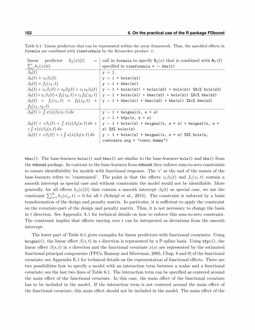
102 6. On the practical use of the R package FDboost
Table 6.1: Linear predictors that can be represented within the array framework. Thus, the specified effects informula are combined with timeformula by the Kronecker product ⊗.
linear predictor hj(x)(t) =∑j hj(x)(t)
call in formula to specify bj(x) that is combined with bY (t)specified in timeformula = ∼ bbs(t)
β0(t) y ∼ 1
β0(t) + z1β1(t) y ∼ 1 + bolsc(z1)
β0(t) + f1(z1, t) y ∼ 1 + bbsc(z1)
β0(t) + z1β1(t) + z2β2(t) + z1z2β3(t) y ∼ 1 + bolsc(z1) + bolsc(z2) + bols(z1) %Xc% bols(z2)
β0(t)+z1β1(t)+f2(z2, t)+z1f3(z2, t) y ∼ 1 + bolsc(z1) + bbsc(z2) + bols(z1) %Xc% bbs(z2)
β0(t) + f1(z1, t) + f2(z2, t) +f3(z1, z2, t)
y ∼ 1 + bbsc(z1) + bbsc(z2) + bbs(z1) %Xc% bbs(z2)
β0(t) +∫x(s)β1(s, t) ds y ∼ 1 + bsignal(x, s = s)
y ∼ 1 + bfpc(x, s = s)
β0(t) + zβ1(t) +∫x(s)β2(s, t) ds +
z∫x(s)β3(s, t) ds
y ∼ 1 + bolsc(z) + bsignal(x, s = s) + bsignal(x, s =
s) %X% bolsc(z)
β0(t) + zβ1(t) + z∫x(s)β4(s, t) ds y ∼ 1 + bolsc(z) + bsignal(x, s = s) %X% bols(z,
contrasts.arg = "contr.dummy")
bbsc(). The base-learners bolsc() and bbsc() are similar to the base-learners bols() and bbs() from
the mboost package. In contrast to the base-learners from mboost they enforce sum-to-zero constraints
to ensure identifiability for models with functional response. The ’c’ at the end of the names of the
base-learners refers to ’constrained’. The point is that the effects z1β1(t) and f1(z1, t) contain a
smooth intercept as special case and without constraints the model would not be identifiable. More
generally, for all effects hj(x)(t) that contain a smooth intercept β0(t) as special case, we use the
constraint∑N
i=1 hj(xij , t) = 0 for all t (Scheipl et al., 2015). The constraint is enforced by a basis
transformation of the design and penalty matrix. In particular, it is sufficient to apply the constraint
on the covariate-part of the design and penalty matrix. Thus, it is not necessary to change the basis
in t direction. See Appendix A.1 for technical details on how to enforce this sum-to-zero constraint.
The constraint implies that effects varying over t can be interpreted as deviations from the smooth
intercept.
The lower part of Table 6.1 gives examples for linear predictors with functional covariates. Using
bsignal(), the linear effect β(s, t) in s direction is represented by a P-spline basis. Using bfpc(), the
linear effect β(s, t) in s direction and the functional covariate x(s) are represented by the estimated
functional principal components (FPCs, Ramsay and Silverman, 2005, Chap. 8 and 9) of the functional
covariate; see Appendix E.1 for technical details on the representation of functional effects. There are
two possibilities how to specify a model with an interaction term between a scalar and a functional
covariate; see the last two lines of Table 6.1. The interaction term can be specified as centered around
the main effect of the functional covariate. In this case, the main effect of the functional covariate
has to be included in the model. If the interaction term is not centered around the main effect of
the functional covariate, this main effect should not be included in the model. The main effect of the
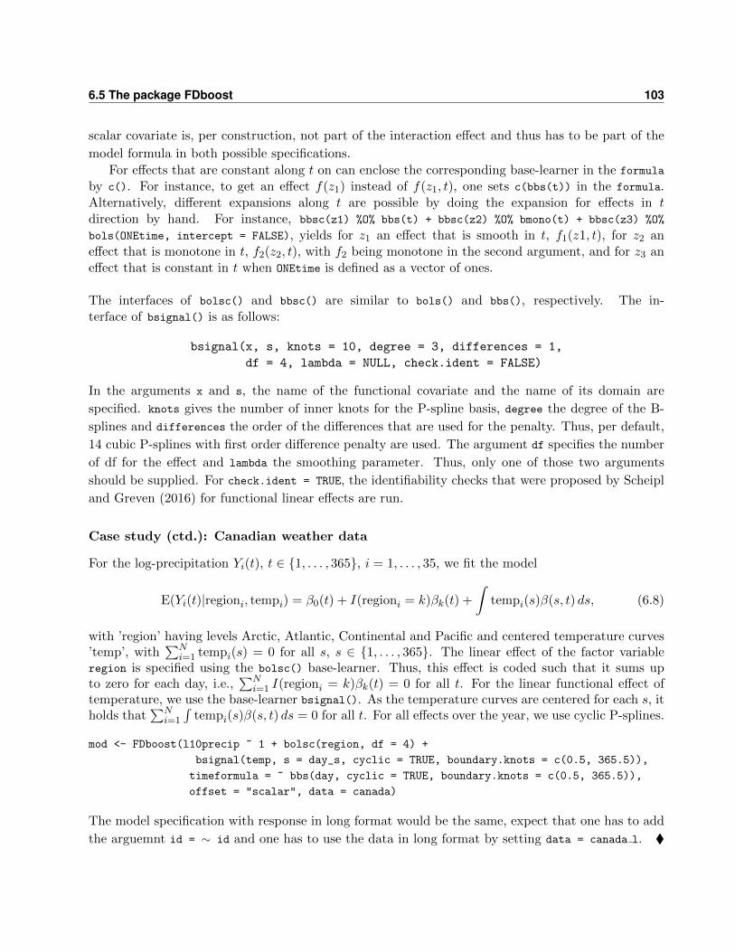
6.5 The package FDboost 103
scalar covariate is, per construction, not part of the interaction effect and thus has to be part of the
model formula in both possible specifications.
For effects that are constant along t on can enclose the corresponding base-learner in the formula
by c(). For instance, to get an effect f(z1) instead of f(z1, t), one sets c(bbs(t)) in the formula.Alternatively, different expansions along t are possible by doing the expansion for effects in tdirection by hand. For instance, bbsc(z1) %O% bbs(t) + bbsc(z2) %O% bmono(t) + bbsc(z3) %O%
bols(ONEtime, intercept = FALSE), yields for z1 an effect that is smooth in t, f1(z1, t), for z2 aneffect that is monotone in t, f2(z2, t), with f2 being monotone in the second argument, and for z3 aneffect that is constant in t when ONEtime is defined as a vector of ones.
The interfaces of bolsc() and bbsc() are similar to bols() and bbs(), respectively. The in-terface of bsignal() is as follows:
bsignal(x, s, knots = 10, degree = 3, differences = 1,
df = 4, lambda = NULL, check.ident = FALSE)
In the arguments x and s, the name of the functional covariate and the name of its domain are
specified. knots gives the number of inner knots for the P-spline basis, degree the degree of the B-
splines and differences the order of the differences that are used for the penalty. Thus, per default,
14 cubic P-splines with first order difference penalty are used. The argument df specifies the number
of df for the effect and lambda the smoothing parameter. Thus, only one of those two arguments
should be supplied. For check.ident = TRUE, the identifiability checks that were proposed by Scheipl
and Greven (2016) for functional linear effects are run.
Case study (ctd.): Canadian weather data
For the log-precipitation Yi(t), t ∈ {1, . . . , 365}, i = 1, . . . , 35, we fit the model
E(Yi(t)|regioni, tempi) = β0(t) + I(regioni = k)βk(t) +
∫tempi(s)β(s, t) ds, (6.8)
with ’region’ having levels Arctic, Atlantic, Continental and Pacific and centered temperature curves’temp’, with
∑Ni=1 tempi(s) = 0 for all s, s ∈ {1, . . . , 365}. The linear effect of the factor variable
region is specified using the bolsc() base-learner. Thus, this effect is coded such that it sums upto zero for each day, i.e.,
∑Ni=1 I(regioni = k)βk(t) = 0 for all t. For the linear functional effect of
temperature, we use the base-learner bsignal(). As the temperature curves are centered for each s, itholds that
∑Ni=1
∫tempi(s)β(s, t) ds = 0 for all t. For all effects over the year, we use cyclic P-splines.
mod <- FDboost(l10precip ~ 1 + bolsc(region, df = 4) +
bsignal(temp, s = day_s, cyclic = TRUE, boundary.knots = c(0.5, 365.5)),
timeformula = ~ bbs(day, cyclic = TRUE, boundary.knots = c(0.5, 365.5)),
offset = "scalar", data = canada)
The model specification with response in long format would be the same, expect that one has to add
the arguemnt id = ∼ id and one has to use the data in long format by setting data = canada l. �

104 6. On the practical use of the R package FDboost
Table 6.2: Linear predictors that contain effects that cannot be separated into an effect in covariate directionand an effect in t direction. These effects in formula are not expanded by the timeformula.
linear predictor hj(x)(t) =∑j hj(x)(t)
call in formula
β0(t) + x(t)β(t) y ∼ 1 + bconcurrent(x, s = s, time = t)
β0(t) +∫ tT1x(s)β(s, t) ds y ∼ 1 + bhist(x, s = s, time = t)
β0(t) +∫ tt−δ x(s)β(s, t) ds y ∼ 1 + bhist(x, s = s, time = t, limits = limitsLag)1
β0(t) +∫ t−δT1
x(s)β(s, t) ds y ∼ 1 + bhist(x, s = s, time = t, limits =
limitsLead)1∫ u(t)l(t) x(s)β(s, t) ds y ∼ 1 + bhist(x, s = s, time = t, limits = mylimits)1
β0(t) + zβ1(t) +∫ tT1x(s)β2(s, t) ds+
z∫ tT1x(s)β3(s, t) ds
y ∼ 1 + bolsc(z) + bhist(x, s = s, time = t) +
bhistx(x) %X% bolsc(z)2
β0(t) + zβ1(t) + z∫ tT1x(s)β2(s, t) ds y ∼ 1 + bolsc(z) + bhistx(x) %X% bols(z, contrasts.arg
= "contr.dummy")2
1 These general limit functions are not defined in FDboost. We give examples for such functions in this paragraph.2 In bhistx(), the variable x has to be of class hmatrix.
Effects in the formula containing the effect in covariate and t direction
If the covariate changes with t, the effect cannot be separated into a marginal basis depending onlyon covariates and a marginal basis depending only on t. Examples for such effects are historicaland concurrent functional effects, as discussed in Chapter 4. In Table 6.2 we give an overview ofpossible linear predictors containing such effects. The concurrent effect β(t)x(t) is only meaningfulif the functional response and the functional covariate are observed over the same domain. Thebase-learner bconcurrent() expands the smooth concurrent effect in P-splines. The historical effect∫ tT1x(s)β(s, t) ds uses only covariate information up to the current observation point of the response.
The base-learner bhist() expands the coefficient surface β(s, t) in s and in t direction using P-splines.In Appendix E.1, details on the representation of functional effects are given. Most arguments ofbhist() are equivalent to those of bsignal(). bhist() has the additional argument time to specifythe observation points of the response. Via the argument limits in bhist() the user can specifyintegration limits depending on t. Per default a historical effect with limits s ≤ t is used. Otherintegration limits can be specified by using a function with arguments s and t that returns TRUE forcombinations of s and t that lie within the integration interval and FALSE otherwise. In the following,we give examples for functions that can be used for limits:
## historical effect; corresponds to default limits = "s<=t"
limitsHist <- function(s, t) {
s <= t
}
## lag effect with lag delta = 5
limitsLag <- function(s, t, delta = 5) {
s >= t - delta & s <= t
}

6.5 The package FDboost 105
## lead effect with lead delta = 5
limitsLead <- function(s, t, delta = 5) {
s <= t - delta
}
The base-learner bhistx() is especially suited to form interaction effects with other base-learners. It
requires the data to be supplied as an object of type hmatrix; see the manual of bhistx() for the
necessary setup.
Case study (ctd.): Canadian weather data
We fit the following model for the log-precipitation with a concurrent effect of temperature:
E(Yi(t)|tempi) = β0(t) + tempi(t)β(t)
A concurrent effect is obtained by the base-learner bconcurrent(), which is not expanded by thebase-learner in timeformula. In this model, timeformula is only used to expand the smooth intercept.
mod_con <- FDboost(l10precip ~ 1 +
bconcurrent(temp, s = day_s, time = day , df = 8,
cyclic = TRUE, boundary.knots = c(0.5, 365.5)),
timeformula = ~ bbs(day, cyclic = TRUE, boundary.knots = c(0.5, 365.5)),
offset = "scalar", data = canada)
Models with concurrent effects can be seen as varying-coefficient models (Hastie and Tibshirani,
1993), where the effect varies over t. �
It is possible to combine effects listed in Table 6.1 and Table 6.2 to form more complex mod-
els. In particular, base-learners with and without array structure can be combined within one model.
As in component-wise boosting each base-learner is evaluated separately, the array structure of the
Kronecker product base-learners can still be exploited in such hybrid models.
Base-learners for scalar response
A scalar response can be seen as special case of a functional response with only one time-point.
Thus, it can be represented as FLAM with basis 1 in time-direction; set timeformula = ∼ bols(1)
or timeformula = NULL for scalar response. In the first call, a Ridge-penalty in t direction is used;
see Chapter 3 for details. With the second call, the scalar response is fitted as scalar response, like
in the function mboost() in package mboost. The advantage of using FDboost() for scalar response is
that base-learners for functional covariates and their associated methods like plot() and coef() are
available.
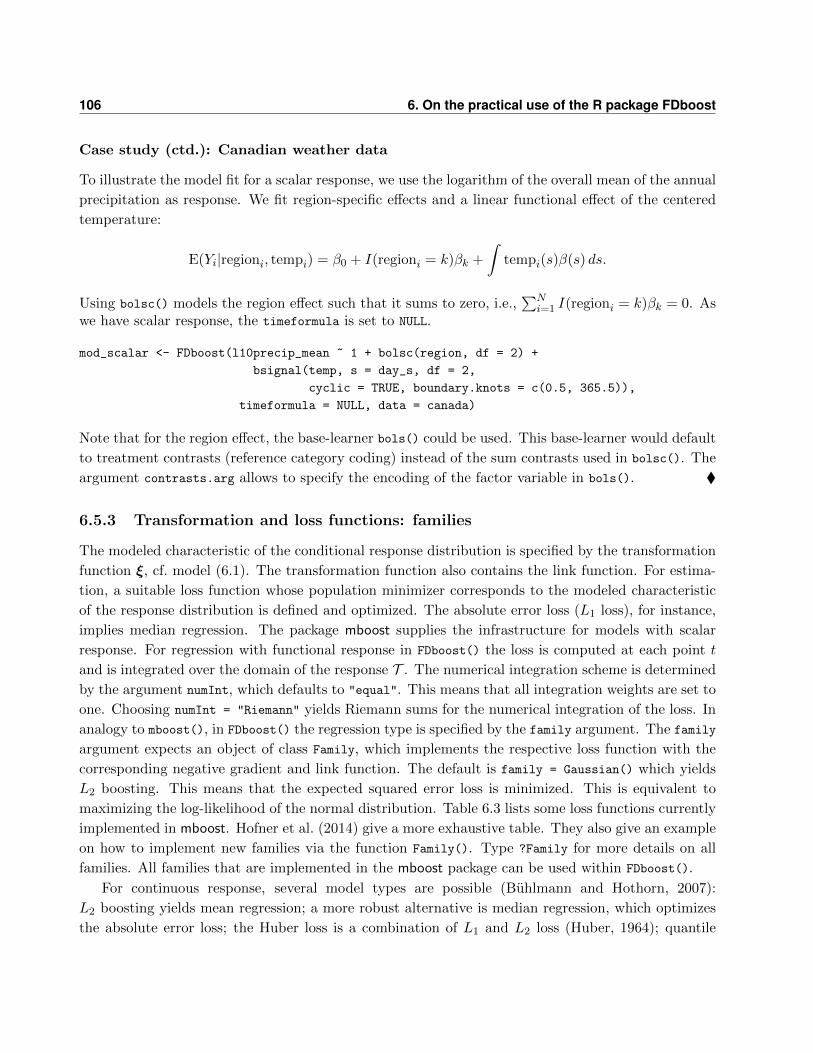
106 6. On the practical use of the R package FDboost
Case study (ctd.): Canadian weather data
To illustrate the model fit for a scalar response, we use the logarithm of the overall mean of the annual
precipitation as response. We fit region-specific effects and a linear functional effect of the centered
temperature:
E(Yi|regioni, tempi) = β0 + I(regioni = k)βk +
∫tempi(s)β(s) ds.
Using bolsc() models the region effect such that it sums to zero, i.e.,∑N
i=1 I(regioni = k)βk = 0. Aswe have scalar response, the timeformula is set to NULL.
mod_scalar <- FDboost(l10precip_mean ~ 1 + bolsc(region, df = 2) +
bsignal(temp, s = day_s, df = 2,
cyclic = TRUE, boundary.knots = c(0.5, 365.5)),
timeformula = NULL, data = canada)
Note that for the region effect, the base-learner bols() could be used. This base-learner would default
to treatment contrasts (reference category coding) instead of the sum contrasts used in bolsc(). The
argument contrasts.arg allows to specify the encoding of the factor variable in bols(). �
6.5.3 Transformation and loss functions: families
The modeled characteristic of the conditional response distribution is specified by the transformation
function ξ, cf. model (6.1). The transformation function also contains the link function. For estima-
tion, a suitable loss function whose population minimizer corresponds to the modeled characteristic
of the response distribution is defined and optimized. The absolute error loss (L1 loss), for instance,
implies median regression. The package mboost supplies the infrastructure for models with scalar
response. For regression with functional response in FDboost() the loss is computed at each point t
and is integrated over the domain of the response T . The numerical integration scheme is determined
by the argument numInt, which defaults to "equal". This means that all integration weights are set to
one. Choosing numInt = "Riemann" yields Riemann sums for the numerical integration of the loss. In
analogy to mboost(), in FDboost() the regression type is specified by the family argument. The family
argument expects an object of class Family, which implements the respective loss function with the
corresponding negative gradient and link function. The default is family = Gaussian() which yields
L2 boosting. This means that the expected squared error loss is minimized. This is equivalent to
maximizing the log-likelihood of the normal distribution. Table 6.3 lists some loss functions currently
implemented in mboost. Hofner et al. (2014) give a more exhaustive table. They also give an example
on how to implement new families via the function Family(). Type ?Family for more details on all
families. All families that are implemented in the mboost package can be used within FDboost().
For continuous response, several model types are possible (Buhlmann and Hothorn, 2007):
L2 boosting yields mean regression; a more robust alternative is median regression, which optimizes
the absolute error loss; the Huber loss is a combination of L1 and L2 loss (Huber, 1964); quantile
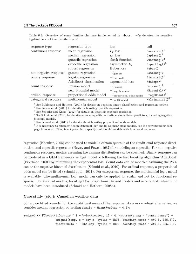
6.5 The package FDboost 107
Table 6.3: Overview of some families that are implemented in mboost. −lF denotes the negativelog-likelihood of the distribution F .
response type regression type loss call
continuous response mean regression L2 loss Gaussian()1
median regression L1 loss Laplace()1
quantile regression check function QuantReg()2
expectile regression asymmetric L2 ExpectReg()3
robust regression Huber loss Huber()1
non-negative response gamma regression −lgamma GammaReg()
binary response logistic regression −lBernoulli Binomial()1
AdaBoost classification exponential loss AdaExp()1
count response Poisson model −lPoisson Poisson()1
neg. binomial model −lneg. binomial NBinomial()4
ordinal response proportional odds model −lproportional odds model ProppOdds()5
categorical response multinomial model −lmultinomial Multinomial()6
1 See Buhlmann and Hothorn (2007) for details on boosting binary classification and regression models.2 See Fenske et al. (2011) for details on boosting quantile regression.3 See Sobotka and Kneib (2012) for details on boosting expectile regression.4 See Schmid et al. (2010) for details on boosting with multi-dimensional linear predictors, including negativebinomial models.5 See Schmid et al. (2011) for details about boosting proportional odds models.6 It is necessary to represent the multinomial logit model as linear array models, see the corresponding helppage in mboost. Thus, is not possible to specify multinomial models with functional response.
regression (Koenker, 2005) can be used to model a certain quantile of the conditional response distri-
bution; and expectile regression (Newey and Powell, 1987) for modeling an expectile. For non-negative
continuous response, models assuming the gamma distribution can be specified. Binary response can
be modeled in a GLM framework as logit model or following the first boosting algorithm ’AdaBoost’
(Friedman, 2001) by minimizing the exponential loss. Count data can be modeled assuming the Pois-
son or the negative binomial distribution (Schmid et al., 2010). For ordinal response, a proportional
odds model can be fitted (Schmid et al., 2011). For categorical response, the multinomial logit model
is available. The multinomial logit model can only be applied for scalar and not for functional re-
sponse. For survival models, boosting Cox proportional hazard models and accelerated failure time
models have been introduced (Schmid and Hothorn, 2008b).
Case study (ctd.): Canadian weather data
So far, we fitted a model for the conditional mean of the response. As a more robust alternative, weconsider median regression by setting family = QuantReg(tau = 0.5):
mod_med <- FDboost(l10precip ~ 1 + bolsc(region, df = 4, contrasts.arg = "contr.dummy") +
bsignal(temp, s = day_s, cyclic = TRUE, boundary.knots = c(0.5, 365.5)),
timeformula = ~ bbs(day, cyclic = TRUE, boundary.knots = c(0.5, 365.5)),

108 6. On the practical use of the R package FDboost
offset = "scalar", data = canada, family = QuantReg(tau = 0.5))
For median regression, the smooth intercept is the estimated median at each day and the effects aredeviations from the median. �
For GAMLSS models, FDboost builds on the package gamboostLSS, in which families to fitGAMLSS are implemented. The families in gamboostLSS need to model at least two distributionparameters–with only one distribution parameter it is a mboost family. For an overview of currentlyimplemented response distributions for GAMLSS, we refer the user to Hofner et al. (2015c). InFDboost, the function FDboostLSS() implements fitting of GAMLSS models with functional data.The interface of FDboostLSS() is:
FDboostLSS(formula, timeformula, id = NULL, data, weights = NULL, ...)
Here, in formula a named list of formulas is supplied. Each list entry in the formula specifies the
potential covariate effects for one of the distribution parameters. Instead of the argument family, the
argument families is used to specify the assumed response distribution with its modeled distribution
parameters. For instance, families = GaussianLSS() yields a Gaussian location scale model. The
model object that is fitted by FDboostLSS() is a list of FDboost model objects. Currently, it is not
possible to automatically fit a smooth offset within FDboostLSS(). All integration weights for the loss
function are set to one, such that all response values are treated as equally important in FDboostLSS().
Case study (ctd.): Canadian weather data
We fit a Gaussian location scale model for the daily log-precipitation Yi(t):
Yi(t) ∼ N(µi(t), σ2i (t)),
µi(t) = β0(t) + I(regioni = k)βk(t) +
∫tempi(s)β(s, t) ds,
log σi(t) = α0(t) + I(regioni = k)αk(t).
The mean is modeled depending on the region and the average temperature curve. The standarddeviation is modeled using a log-link as varying over the year with a region-specific effect. Theformula has to be specified as a list of two formulas with names mu and sigma for mean and standarddeviation of the normal distribution.
library(gamboostLSS)
## Gaussian location scale model
mod_ls <- FDboostLSS(list(mu = l10precip ~ 1 + bolsc(region, df = 4) +
bsignal(temp, s = day_s, cyclic = TRUE,
boundary.knots = c(0.5, 365.5), df = 4),
sigma = l10precip ~ 1 + bolsc(region, df = 4)),
timeformula = ~ bbs(day, cyclic = TRUE,
boundary.knots = c(0.5, 365.5), df = 3),

6.5 The package FDboost 109
data = canada, families = GaussianLSS())
## print mean model
mod_ls$mu
## print model for standard deviation
mod_ls$sigma
Note that the effects in the formulas for mu and for sigma are all expanded by timeformula. �
6.5.4 Model tuning and early stopping
Boosting iteratively selects base-learners to update the linear predictor. Fixing the base-learners and
the step-length, the model complexity is controlled by the number of boosting iterations. With more
boosting iterations the model gets more complex. To ensure a fair selection of base-learners, it is
important to specify equal df for each base-learner. If not, selection is biased towards more flexible
base-learners with higher df as they are more likely to yield larger improvements of the fit in each
iteration, see Hofner et al. (2011) for details. Each base-learner has an argument df that allows to
fix the df prior to the model fit. In FDboost() care has to be taken as some base-learners in the
formula are expanded by the base-learner in timeformula, but other are not. All base-learners listed
in Table 6.1 are expanded by timeformula. The base-learners given in Table 6.2 contain the effect in
covariate and in t direction and are not expanded by the timeformula. For the row tensor product
or the Kronecker product of two base-learners, the df for the combined base-learner is computed as
product of the two marginally specified df. For instance, formula = y ∼ bbsc(z, df = 3) + bhist(x,
s = s, df = 12) and timeformula = ∼ bbs(t, df = 4) implies 3 ∗ 4 = 12 df for the first combined
base-learner and 12 df for the second base-learner. The call extract(object, "df") displays the df
for each base-learner in a FDboost object.
The step-length ν is chosen sufficiently small from the interval (0, 1), e.g., as ν = 0.1, which is also
the default. For smaller step-length, more boosting iterations are required and vice versa (Friedman,
2001). Note that the default number of boosting iterations is 100. This is arbitrary and in most
cases not adequate. The number of boosting iterations and the step-length of the algorithm can be
specified in the argument control. This argument must be supplied as a call to boost control(). For
example, control = boost control(mstop = 50, nu = 0.2) implies 50 boosting iterations and step-
length ν = 0.2.
We choose the optimal number of boosting iterations by resampling methods like cross-validation
or bootstrapping. In the package FDboost, three different functions for estimating the optimal stop-
ping iteration by resampling exist. Depending on the specified model, some parameters are computed
from the data prior to the model fit: for functional response, per default a smooth functional offset
β∗0(t) is computed (for offset = NULL in FDboost()); for linear and smooth effects of scalar variables
computed by bolsc() and bbsc() transformation matrices Zj for the sum-to-zero constraints are
computed. The resampling functions differ in what is recomputed in each resampling fold. Thus,
they also differ in computational efficiency.The function cvrisk.FDboost() directly calls cvrisk.mboost() from the mboost package, which is
very efficient. For all folds in cvrisk.FDboost(), the smooth functional offset and the transformation

110 6. On the practical use of the R package FDboost
matrices for the sum-to-zero constraints from the model fitted on all data are used. Thus, these pa-rameters are treated as fixed and the uncertainty induced by their estimation is not considered in theresampling. Per default only the out-of-bag risk is returned. The function validateFDboost() recom-putes the smooth offset in each fold. Next to the out-of-bag risk, validateFDboost() also returns theestimated coefficients for all folds. These estimated coefficients can be used to access the variability ofthe estimates. But due to the extra computations, validateFDboost() is much more time and mem-ory consuming than cvrisk.FDboost(). The function applyFolds() recomputes the smooth offset andthe transformation matrices and only returns the out-of-bag risk. Thus, it is computationally moreefficient than validateFDboost(). For scalar response, the function cvrisk.FDboost() can be usedand the other two functions yield the same optimal stopping iteration. For functional response, theresampling methods are equal if no smooth offset and no base-learner implying an identifiability con-straint is used (bolsc() and bbsc()). For these cases, we recommend to use the function applyFolds()
to determine the optimal number of boosting iterations. The interface of applyFolds() is:
applyFolds(object,
folds = cv(rep(1, length(unique(object$id))), type = "bootstrap"),
grid = 1:mstop(object))
In the argument object, the fitted model object is specified. grid defines the grid on which the optimalstopping iteration is searched. Via argument folds the resampling folds are defined by suitableweights. Per default, 25-fold bootstrap is used. The functions validateFDboost() and applyFolds()
expect resampling weights that are defined on the level of curves. That means, the folds must containweights wi, i = 1, . . . , N . The function cvrisk.FDboost() expects resampling weights on the level ofsingle observations, i.e., weights wig, i = 1, . . . , N , g = 1, . . . , Gi. To set up the resampling folds, thefunction cv() from package mboost can be used, which has the interface:
cv(weights, type = c("bootstrap", "kfold", "subsampling"),
B = ifelse(type == "kfold", 10, 25))
The argument weights is used to specify the weights of the original model. Via argument type
the resampling scheme is defined: ”bootstrap” for bootstrapping, ”kfold” for cross-validation and
”subsampling” means resampling in each fold half of the observations. The number of folds is set
by B. Per default, 10 folds are used for cross-validation and 25 folds for bootstrapping and subsampling.
Case study (ctd.): Canadian weather data
We search the optimal stopping iteration for model (6.8) by a 10-fold bootstrap.
## create folds for 10-fold bootstrap: one weight for each curve
set.seed(123)
folds_bs <- cv(weights = rep(1, mod$ydim[1]), type = "bootstrap", B = 10)
## compute out-of-bag risk on the 10 folds for 1 to 200 boosting iterations
cvr <- applyFolds(mod, folds = folds_bs, grid = 1:200)
## compute out-of-bag risk and coefficient estimates on folds

6.5 The package FDboost 111
cvr2 <- validateFDboost(mod, folds = folds_bs, grid = 1:200)
## weights per observation point
folds_bs_long <- folds_bs[rep(1:nrow(folds_bs), times = mod$ydim[2]), ]
attr(folds_bs_long, "type") <- "10-fold bootstrap"
## compute out-of-bag risk on the 10 folds for 1 to 200 boosting iterations
cvr3 <- cvrisk(mod, folds = folds_bs_long, grid = 1:200)
The estimated out-of-bag risks are slightly different, as in applyFolds() the matrix for the identifia-
bility constraint in bolsc() is recomputed in each fold and in validateFDboost() and cvrisk() the
transformation matrix is used as computed on the whole dataset. �
The variable selection can be refined using stability selection (Meinshausen and Buhlmann,
2010). Stability selection is a procedure to select influential variables while controlling false discovery
rates and maximal model complexity. For component-wise gradient boosting, it is implemented in
mboost in the function stabsel() (Hofner et al., 2015a). For functional response, care has to be
taken to do the resampling on the level of curves.
6.5.5 Methods to extract and display results
Methods to extract and display results of the fitted models and of the resampling procedures have been
implemented. The resampling results of applyFolds() and cvrisk() have class cvrisk. The resampling
results of validateFDboost() are of the class validateFDboost. For all resampling objects, the method
mstop() extracts the estimated optimal number of boosting iterations. plot() generates a plot of
the estimated out-of-bag risk per stopping iteration in each fold. With this plot, the convergence
behavior can be graphically examined. If the resampling is conducted by validateFDboost(), the
function plotPredCoef() can be used to plot the coefficient estimates of all folds.
Case study (ctd.): Canadian weather data
We generate a plot that displays for each fold the estimated out-of-bag risk per stopping iteration;see Figure 6.1. The estimated optimal number of stopping iterations is accessed by mstop(). For thevalidateFDboost() object, we plot the coefficients estimated in each bootstrap folds; see Figure 6.2for the bootstrapped coefficient estimates of the variable region.
#### plot for each fold the estimated out-of-bag risk per stopping iteration
par(mfrow = c(1,3))
plot(cvr); legend("topright", lty=2, paste(mstop(cvr)))
plot(cvr2)
plot(cvr3); legend("topright", lty=2, paste(mstop(cvr3)))
#### access the estimated optimal stopping iteration
mstop(cvr)
mstop(cvr2)
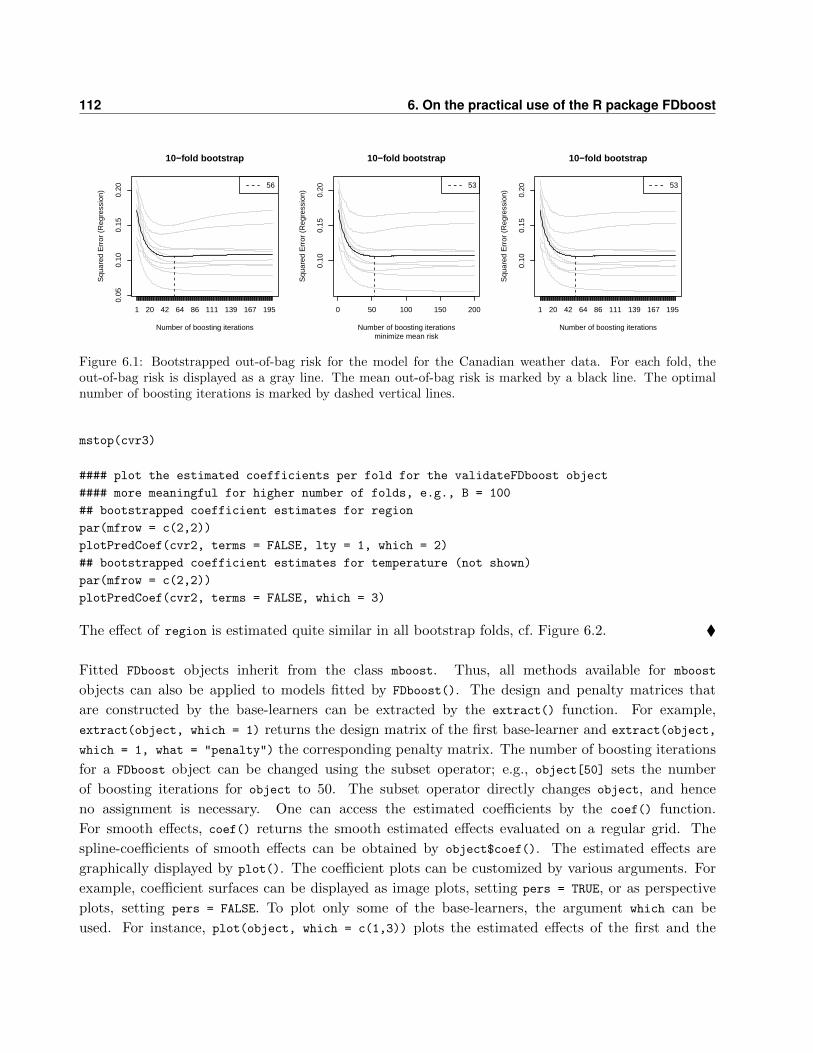
112 6. On the practical use of the R package FDboost
10−fold bootstrap
Number of boosting iterations
Squ
ared
Err
or (
Reg
ress
ion)
1 20 42 64 86 111 139 167 195
0.05
0.10
0.15
0.20 56
0 50 100 150 2000.
100.
150.
20
10−fold bootstrap
minimize mean riskNumber of boosting iterations
Squ
ared
Err
or (
Reg
ress
ion)
53
10−fold bootstrap
Number of boosting iterations
Squ
ared
Err
or (
Reg
ress
ion)
1 20 42 64 86 111 139 167 195
0.10
0.15
0.20 53
Figure 6.1: Bootstrapped out-of-bag risk for the model for the Canadian weather data. For each fold, theout-of-bag risk is displayed as a gray line. The mean out-of-bag risk is marked by a black line. The optimalnumber of boosting iterations is marked by dashed vertical lines.
mstop(cvr3)
#### plot the estimated coefficients per fold for the validateFDboost object
#### more meaningful for higher number of folds, e.g., B = 100
## bootstrapped coefficient estimates for region
par(mfrow = c(2,2))
plotPredCoef(cvr2, terms = FALSE, lty = 1, which = 2)
## bootstrapped coefficient estimates for temperature (not shown)
par(mfrow = c(2,2))
plotPredCoef(cvr2, terms = FALSE, which = 3)
The effect of region is estimated quite similar in all bootstrap folds, cf. Figure 6.2. �
Fitted FDboost objects inherit from the class mboost. Thus, all methods available for mboost
objects can also be applied to models fitted by FDboost(). The design and penalty matrices that
are constructed by the base-learners can be extracted by the extract() function. For example,
extract(object, which = 1) returns the design matrix of the first base-learner and extract(object,
which = 1, what = "penalty") the corresponding penalty matrix. The number of boosting iterations
for a FDboost object can be changed using the subset operator; e.g., object[50] sets the number
of boosting iterations for object to 50. The subset operator directly changes object, and hence
no assignment is necessary. One can access the estimated coefficients by the coef() function.
For smooth effects, coef() returns the smooth estimated effects evaluated on a regular grid. The
spline-coefficients of smooth effects can be obtained by object$coef(). The estimated effects are
graphically displayed by plot(). The coefficient plots can be customized by various arguments. For
example, coefficient surfaces can be displayed as image plots, setting pers = TRUE, or as perspective
plots, setting pers = FALSE. To plot only some of the base-learners, the argument which can be
used. For instance, plot(object, which = c(1,3)) plots the estimated effects of the first and the
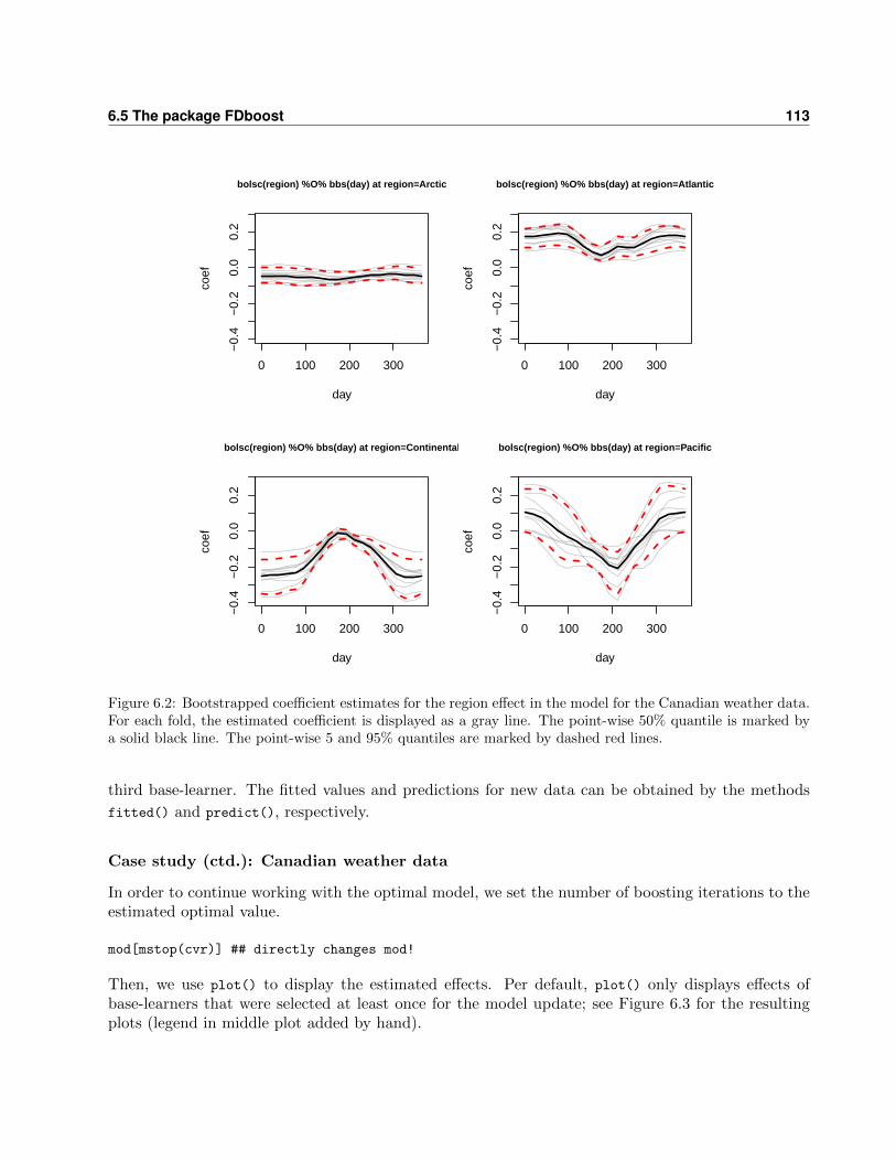
6.5 The package FDboost 113
0 100 200 300
−0.
4−
0.2
0.0
0.2
bolsc(region) %O% bbs(day) at region=Arctic
day
coef
0 100 200 300
−0.
4−
0.2
0.0
0.2
bolsc(region) %O% bbs(day) at region=Atlantic
day
coef
0 100 200 300
−0.
4−
0.2
0.0
0.2
bolsc(region) %O% bbs(day) at region=Continental
day
coef
0 100 200 300
−0.
4−
0.2
0.0
0.2
bolsc(region) %O% bbs(day) at region=Pacific
day
coef
Figure 6.2: Bootstrapped coefficient estimates for the region effect in the model for the Canadian weather data.For each fold, the estimated coefficient is displayed as a gray line. The point-wise 50% quantile is marked bya solid black line. The point-wise 5 and 95% quantiles are marked by dashed red lines.
third base-learner. The fitted values and predictions for new data can be obtained by the methods
fitted() and predict(), respectively.
Case study (ctd.): Canadian weather data
In order to continue working with the optimal model, we set the number of boosting iterations to theestimated optimal value.
mod[mstop(cvr)] ## directly changes mod!
Then, we use plot() to display the estimated effects. Per default, plot() only displays effects ofbase-learners that were selected at least once for the model update; see Figure 6.3 for the resultingplots (legend in middle plot added by hand).
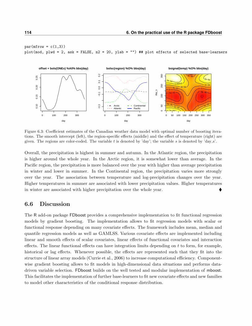
114 6. On the practical use of the R package FDboost
par(mfrow = c(1,3))
plot(mod, plwd = 2, ask = FALSE, n2 = 20, ylab = "") ## plot effects of selected base-learners
0 100 200 300
0.10
0.15
0.20
0.25
offset + bols(ONEx) %A0% bbs(day)
day
0 100 200 300
−0.
3−
0.1
0.0
0.1
0.2
bolsc(region) %O% bbs(day)
day
ArcticAtlantic
ContinentalPacific
0 50 100 150 200 250 300 350
050
150
250
350
bsignal(temp) %O% bbs(day)
day
day_
s
−5e−05 −5e−05
0 0
0 5e−05
5e−05
5e−05
5e−05 1e−04
1e−04 1e−04 0.00015
2e−04
2e−04 2e−04
Figure 6.3: Coefficient estimates of the Canadian weather data model with optimal number of boosting itera-tions. The smooth intercept (left), the region-specific effects (middle) and the effect of temperature (right) aregiven. The regions are color-coded. The variable t is denoted by ’day’; the variable s is denoted by ’day s’.
Overall, the precipitation is highest in summer and autumn. In the Atlantic region, the precipitation
is higher around the whole year. In the Arctic region, it is somewhat lower than average. In the
Pacific region, the precipitation is more balanced over the year with higher than average precipitation
in winter and lower in summer. In the Continental region, the precipitation varies more strongly
over the year. The association between temperature and log-precipitation changes over the year.
Higher temperatures in summer are associated with lower precipitation values. Higher temperatures
in winter are associated with higher precipitation over the whole year. �
6.6 Discussion
The R add-on package FDboost provides a comprehensive implementation to fit functional regression
models by gradient boosting. The implementation allows to fit regression models with scalar or
functional response depending on many covariate effects. The framework includes mean, median and
quantile regression models as well as GAMLSS. Various covariate effects are implemented including
linear and smooth effects of scalar covariates, linear effects of functional covariates and interaction
effects. The linear functional effects can have integration limits depending on t to form, for example,
historical or lag effects. Whenever possible, the effects are represented such that they fit into the
structure of linear array models (Currie et al., 2006) to increase computational efficiency. Component-
wise gradient boosting allows to fit models in high-dimensional data situations and performs data-
driven variable selection. FDboost builds on the well tested and modular implementation of mboost.
This facilitates the implementation of further base-learners to fit new covariate effects and new families
to model other characteristics of the conditional response distribution.
Chapter 7
Discussion
In this concluding chapter an overall summary is given that highlights the main developments of the
thesis. For a more thorough discussion of the modeling aspects treated in the Chapters 3, 4 and 5,
we refer to the discussion within the corresponding chapter. Additionally, starting points for future
research directions are discussed.
7.1 Concluding summary
Regression models for functional data are versatile tools, which can be used in applications from
many scientific fields. Moreover, these models are becoming increasingly important as technological
advances make functional data more common. In this thesis, a generic framework for regression
with functional data is developed, with the estimation conducted by boosting. The idea for widely
applicable functional regression models with many covariate effects is based on Scheipl et al. (2015).
We adapt the component-wise gradient boosting algorithm of Buhlmann and Hothorn (2007) and
Hothorn et al. (2013) for functional response and implement new base-learners for functional co-
variates. The benefits of using a component-wise gradient boosting algorithm to estimate functional
regression models are (a) the possibility for modeling one of multiple characteristics of the conditional
response distribution, including the expectation, quantiles and expectiles, as well as the possibility
to model several distribution parameters simultaneously in a GAMLSS framework, (b) the feasibility
of estimation in high-dimensional data settings, even with more covariates than observations, (c) the
regularization of effect estimates that leads to shrinkage in the estimation and more stable predictions,
(d) data-driven variable selection and (e) the availability of an efficient implementation. Furthermore,
the modular structure of the modeling framework and its implementation invites further extensions.
One limitation is that boosting–in contrast to Bayesian or maximum likelihood-based estimation
frameworks–does not directly provide inference such as p-values or confidence intervals. The problem
is that shrinkage of the estimated effects makes the construction of confidence intervals and signif-
icance tests difficult. The lack of formal inference can be addressed by methods like bootstrapping
and permutation tests. For example, the uncertainty of the estimated coefficients can be accessed by
116 7. Discussion
non-parametric bootstrap. In order to select relevant variables, it is possible to use stability selection
(Meinshausen and Buhlmann, 2010) in combination with boosting.
Various aspects of the general modeling framework are examined in more detail. In particular,
we discuss:
• the general modeling framework, into which all considered models can be embedded (Chapter 2).
• the functional linear array model (FLAM) for functional response observed on one common grid
and covariates that do not vary over the domain of the response (Chapter 3).
• models for functional response observed on irregular grids and/or covariates that vary over the
domain of the response, as in models with functional historical effects (Chapter 4).
• the combination of scalar-on-function regression and GAMLSS (generalized additive models for
location scale and shape) for modeling several parameters of the conditional response distribu-
tion simultaneously (Chapter 5).
• the implementation of the proposed framework in the R package FDboost (Chapter 6).
As a starting point, we define a structured additive regression model that represents the generic
framework in Chapter 2. All models that are discussed within this thesis can be embedded within
this generic modeling framework.
In Chapter 3, functional regression models for responses that are observed on one common grid
are represented as linear array models (Currie et al., 2006). The common observation grid makes
it possible to store the response in a matrix. Because this is a two-dimensional array, array models
can be used. We call this type of model a functional linear array model (FLAM). Taking advan-
tage of the Kronecker product in the design matrix makes array framework computationally efficient.
The FLAM is applied in three settings: to model the viscosity of resin over time depending on
experimental conditions (function-on-scalar); to predict the heat value of fossil fuels using spectral
measurements (scalar-on-function); and to relate the average yearly precipitation curve to the aver-
age yearly temperature curve, the climatic zone and the location of the weather station in Canada
(function-on-function).
Motivated by a biotechnological data set on fermentation processes, we consider models that do
not rely on the array structure (Chapter 4). This allows for more flexible model specifications at the
expense of loosing computational efficiency. In particular, models for irregularly observed functional
responses and effects of covariates that vary along the domain of the response are feasible. The aim
is to predict a key process parameter of the fermentation process that is too time-consuming to be
determined during new fermentations by easily accessible process variables that can be measured in
real time. To this end, we use a functional regression model with many historical effects.
To further increase the flexibility of the modeling framework, we then combine scalar-on-function
regression and GAMLSS (Chapter 5). For this model, we also discuss estimation by penalized max-
imum likelihood methods based on Rigby and Stasinopoulos (2005) and Wood et al. (2015). We
7.2 Outlook 117
simultaneously model expectation and variance of a time-series on stock returns depending on func-
tional liquidity measures.
A comprehensive implementation of the methods is provided in the R package FDboost (Brockhaus
and Rugamer, 2016), which relies on the fitting machine of the mboost package (Hothorn et al., 2016).
The thesis contains a short tutorial on how to use the software for fitting functional regression models,
discussing model set-up and model choice (Chapter 6).
7.2 Outlook
To extend the proposed functional regression framework two main directions can be followed. It is
possible to apply other loss functions yielding models for other features of the conditional response
distribution or to implement new base-learners for novel covariate effects.
Extensions through new loss functions and corresponding transformation functions. As briefly
touched upon in Brockhaus et al. (2015a) it is possible to combine regression models for functional
response and GAMLSS. This is done by integrating the loss function, which for GAMLSS is the
negative log-likelihood, along the domain of the response. Because of the smoothness assumption
along the domain of the response, the conditional response distribution is estimated to be similar for
close observation points. However, covariance along the domain of the response cannot be captured
by the model. Almond Stocker (Department of Statistics, LMU Munich) deals within his master
thesis with the combination of functional response regression and GAMLSS (ongoing work).
Another idea is to extend functional regression models by combining them with conditional trans-
formation models (CTMs, Hothorn et al., 2013). CTMs model the whole conditional response distri-
bution depending on covariates in a semi-parametric way. Instead of assuming a specific distribution,
a CTM directly models the conditional distribution function, which implies all characteristics of the
distribution including moments and quantiles. The use of CTMs for scalar response and functional
covariates is straightforward. An estimation of CTMs by gradient boosting is implemented in the
R package ctm (Hothorn, 2013). This package can be used in combination with base-learners for
functional covariates in the FDboost package. CTMs for functional response can be achieved by
integrating the loss along the domain of the response. This only models the conditional response
distribution at each point of the domain of the response.
To obtain loss functions suitable for functional response, so far, we compute the loss at each
observation point and integrate over the domain of the response. Instead of integrating a loss function
that is suited for scalar response, it is possible to think of loss functions especially suited to functional
data. One idea is to construct loss functions from functional depth functions, e.g., using the band
depth of Lopez-Pintado and Romo (2009). In this setting, a loss function could be constructed as the
relative frequency of discordant pairs.
Another direction for future research is regression models for functional response that has higher
dimension; for instance, image regression (Crainiceanu et al., 2012; Zipunnikov et al., 2014).
118 7. Discussion
Extensions through new base-learners. It is possible to construct base-learners for further interaction
effects. Including next to the main effects an interaction effect for two scalar covariates, care has
to be taken to ensure identifiability of the model terms. Consider two factor variables, z1 and z2,
with main effects, I(z1 = k)αk(t) and I(z2 = l)βl(t), and interaction effect I(z1 = k)I(z2 = l)γkl(t).
Identifiability of such effects can be obtained by using suitable sum-to-zero constrains at each point
of the domain of the functional response. For the main effects, identifiability is ensured by centering
the effects around the functional intercept, see Appendix A.1. The interaction effect has to be
centered around the functional intercept as well as the two main effects; this is enforced by additional
constraints. Moreover, interaction effects between scalar and functional covariates are possible,
for instance, group-specific functional historical effects, I(z = k)∫ u(t)l(t) x(s)γk(s, t) ds. When also
including the main effects, I(z = k)αk(t) and∫ u(t)l(t) x(s)β(s, t) ds, in the model, similar identifiability
constraints are necessary. In this context, it can also be of interest to allow for anisotropic penalty
matrices that use more than one smoothing parameter. For example, different amounts of smoothing
can be specified for the two covariates in an interaction term. Rugamer et al. (2016) thoroughly
discusses such interaction effects with one or two factor variables and functional covariate for
modeling the relation between EEG (electroencephalography) and EMG (electromyography) signals
under various experimental conditions. In scalar-on-function regression, an interaction effect between
two functional covariates can be specified as∫∫
x1(s1)x2(s2)β(s1, s2) ds1ds2 (Fuchs et al., 2015;
Usset et al., 2016). Such effects conceptually fit into the array framework and could be extended to
functional response regression.
Another interesting direction for future research is to develop base-learners for functional effects
that select relevant regions of the functional covariates. This can be achieved by coefficient functions
for which only relevant parts are estimated to be unequal zero and the other parts are set to zero.
James et al. (2009) and Tutz and Gertheiss (2010) consider such sparse effects for a linear effect
of a functional covariate on a scalar response. In future work, such effects might be included in
our framework or even extended to effect surfaces of linear effects in function-on-function regression
models. In the context of functional historical effects or lag effects a potentially plausible assumption
is that the effect gets smaller for bigger lag. This can be encoded by imposing a penalty towards
zero for the maximal used lag; see Obermeier et al. (2014) for an approach using such a penalty in
a distributed lag model. For a functional historical effect,∫ tT1x(s)β(s, t) ds, the penalty towards zero
would have to be at the edge of the coefficient surface with minimal s and maximal t such that the
effect gets smaller for bigger differences between the observation point s of the covariate and the
observation point t of the response.
Additionally, the available basis functions could be extended to other basis functions than P-
splines and FPCs. For example, using a thin plate regression spline basis (Wood, 2003) could be
beneficial for the estimation of coefficient surfaces that do not have rectangular support, which is the
case for functional historical effects.
Leaving the linearity assumption, it is possible to consider a non-linear functional effect∫S f(x(s), s) ds, where f is a smooth unknown function to be estimated from the data (Muller et al.,

7.2 Outlook 119
2013; McLean et al., 2014). The basis and penalty specification of McLean et al. (2014) could be
directly translated to a new base-learner. For functional response and covariate both observed on
the same domain, Kim et al. (2016) propose a non-linear concurrent effect f(x(t), t), with smooth
unknown function f , which could also be translated to a new base-learner.
Another interesting extension would be to include base-learners for higher-dimensional functional
variables like images; see Goldsmith et al. (2014) for scalar-on-image regression.
Overall, functional regression models are a wide field with many challenges. I hope that this
thesis is a contribution towards flexible and widely applicable regression models for functional data.

120 7. Discussion

Appendices


Appendix A
Identifiability
Appendix A.1 is based on Web Appendix A of the following paper:
Brockhaus, S., Scheipl, F., Hothorn, T., and Greven, S. (2015): The functional linear
array model. Statistical Modelling, 15(3), 279–300.
Appendix A.2 is based on Web Appendix A of the following paper:
Brockhaus, S., Melcher, M., Leisch, F., and Greven, S. (2016): Boosting flexible func-
tional regression models with a high number of functional historical effects. Statistics and
Computing, accepted, DOI: http://dx.doi.org/10.1007/s11222-016-9662-1.
We consider identifiability for functional responses and for functional covariates. In the case of func-
tional response (see Section A.1), identifiability can be ensured by suitable sum-to-zero constraints.
This works similar to choosing dummy or effect coding of factor variables in a simple linear model
where the chosen constraints ensure an identifiable model and determine the interpretation of the
intercept and of the covariate effects. Transferring this to functional responses Y (t), the constraints
are enforced at each point t (Scheipl et al., 2015). For functional covariates (see Section A.2), a
different kind of identifiability problem can arise. If a functional covariate does not carry enough
information, it can happen that the model given the covariate is not identifiable. Scheipl and Greven
(2016) discuss this identifiability issue and possible solutions for linear functional effects with fixed
integration limits. In Chapter 4, we transfer this to functional effects with t-specific integration limits.
A.1 Functional response: identifiability constraints for FLAMs
Consider a model ξ(Yi(t)) = β0(t) +hj(xi)(t), with smooth intercept β0(t) and an effect hj(x)(t) that
contains an intercept β0(t) as special case. For the effects in Table 2.1, this is the case for the smooth
124 A. Identifiability
effect f(z, t) and smooth interaction f(z1, z2, t), the group-specific intercept bg(t) and smooth residual
ei(t). The problem is that such a model is not identifiable as
ξ(Yi(t)) = β0(t) + hj(xi)(t)
=[β0(t) + hj(x)(t)
]+[hj(xi)(t)− hj(x)(t)
]= β0(t) + hj(x)(t),
yields the same fit with a different parametrization for hj(x)(t) = EX(hj(X)(t)), or replacing the
expectation by the mean for concrete data, for hj(x)(t) = N−1∑
i hj(xi)(t). Scheipl et al. (2015)
pointed out that standard sum-to-zero constraints∑
i,t hj(xi)(t) = 0 are not suitable for regression
models with functional response. A suitable constraint is that the mean effect of each covariate should
be zero in each point t:
N−1∑
ihj(xi)(t) = 0 ∀t.
We now show how to embed this constraint within the array framework of the FLAM. We define B as
the NG×KYKj design matrix with rows(bj(xi)
> ⊗ bY (tg)>) defined as in equation (3.2). B is the
tensor product of the two marginal design matrices B = Bj ⊗BY , with Bj having bj(xi)> as rows
and BY having bY (tg)> as rows. In this notation the response would be concatenated to a 1 ×NG
vector (Y1(t1), . . . , YN (tG))>. Then the sum-to-zero constraint over t can be represented as a linear
constraint on the coefficient vector by enforcing Cθ = 0, with C = (1>N ⊗ IG)B, where 1N is the
vector of length N containing ones and IG is the G-dimensional identity matrix. Wood (2006, sec.
1.8.1) implements linear constraints by rewriting the model in terms of KY (Kj − 1) unconstrained
parameters through a change of basis for the design matrix B. For this, the full QR decomposition
of C> is needed:
C> = [Q : Z]
[R
0
]= QR,
where [Q : Z] forms a KYKj×KYKj orthonormal matrix and R is a G×G upper triangular matrix.
The transformed design matrix is obtained by the multiplication of the original design matrix with
the transformation matrix Z yielding BZ.
To apply this method for implementing a linear constraint in a FLAM, it is necessary to do the
transformation on the marginal design matrices BY and Bj . Therefore we rewrite C> depending on
the marginal bases as C> = ((1>N⊗IG)(Bj⊗BY ))> = (B>j 1N )⊗B>Y and use the QR decompositions
of B>j 1N and B>Y whose components are indexed by j and Y respectively:
C> =
([Qj : Zj ]
[Rj
0
])⊗
([QY : ZY ]
[RY
0
])
= ([Qj : Zj ]⊗ [QY : ZY ])
([Rj
0
]⊗
[RY
0
])= [Q : Z]
[R
0
].

A.2 Functional covariates: identifiability of historical effects 125
Thus we can calculate the transformation matrix Z as Z = (Zj ⊗ [QY : ZY ]) and we obtain the
transformed design matrix as
BZ = (Bj ⊗BY )(Zj ⊗ [QY : ZY ]) = (BjZj)⊗ (BY [QY : ZY ]).
As multiplication by the orthonormal matrix [QY : ZY ] only rotates the basis, this rotation can
be omitted. Thus only the transformation by Zj is necessary and it suffices to compute the QR
decomposition of B>j 1N ∈ RKj×1. It is not necessary to compute the QR decomposition of the
complete design matrix B or even to construct B explicitly. A basis transformation of the design
matrix, BjZj , involves that the penalty matrix P j has to be transformed accordingly to Z>j P jZj .
Please note that while unrelated to identifiability, centering the covariates by subtracting their
mean (function) can in some cases additionally lend itself to nice interpretations of the intercept as
the overall mean.
A.2 Functional covariates: identifiability of historical effects
A.2.1 Marginal design matrices
Consider a regular design where the N responses Y = [yi(tg)] i=1,...,Ng=1,...,G
and the functional covariate
Xj = [xij(sr)] i=1,...,Nr=1,...,R
are both observed on a common grid with G and R observation points respec-
tively. For simplicity of notation, we use a model with one functional effect. The unconstrained and
the constrained functional model can be represented using a row tensor product, see equation (4.9),
ξ(vec( YN×G
)) ≈
([{HNG×R
· (XjN×R
∆R×R
⊗ 1GG×1
)
}Φs
R×Kj
]�
[1NN×1
⊗ ΦtG×KY
])θ
KjKY ×1
(A.1)
= (Bj �BY )θ, (A.2)
where vec(Y ) is the vectorization of the response matrix, Φs and Φt are basis matrices of Kj and
KY basis functions evaluated in (s1, . . . , sR) and (t1, . . . , tG) respectively, ∆ is a diagonal matrix of
integration weights ∆(sr), H is a matrix of zeros and ones to implement the integration limits as
functions in t and θ is the vector of coefficients. Note, that the marginal design matrices Bj and
BY are defined by equation (A.2).
Unconstrained functional effect. The unconstrained functional effect corresponds to the special
case with integration limits {T1, T2} and is achieved in model (A.1) by setting all entries of H to one.
Thus, H can be omitted, eliminating the dependency of Bj on t. In that case the mixed product
rule (Brewer, 1978) gives the equality (Xj∆ ⊗ 1G)Φs = (Xj∆Φs) ⊗ 1G. Setting Dj = Xj∆Φs
and DY = Φt, the design matrix is the Kronecker product of those two marginal design matrices,
(Dj ⊗ 1G) � (1N ⊗DY ) = Dj ⊗DY . The matrix Dj is the marginal design matrix in direction of
the covariate for the unconstrained functional effect.

126 A. Identifiability
Constrained functional effect. To represent a constrained functional effect using model (A.1),
the matrix H contains zeros and ones implementing the desired integration limits and is defined as
H = [hig,r] ig=11,...,NGr=1,...,R
, with hig,r = I (l(tg) ≤ sr ≤ u(tg)). The marginal design matrices can then be
written as
Bj =
[R∑r=1
hig,rxij(sr)∆(sr)Φk(sr)
]ig=11,...,NGk=1,...,Kj
= [(Bj)ig,k] ig=11,...,NGk=1,...,Kj
and
BY = [Φl(tg)] ig=11,...,NGl=1,...,KY
corresponding to equation (A.1). The marginal design matrices can easily be adjusted for the case
where the response is observed on curve-specific grids (ti1, . . . , tiGi)>. As one common observation grid
for all response curves simplifies the notation considerably and the generalization to curve-specific
grids is technical, we focus on the first case. The necessary adaptions for curve-specific grids are
treated in Subsection A.2.4.
A.2.2 Checking for rank deficiency of the design matrix
Unconstrained functional effect. As proposed by Scheipl and Greven (2016), we check whether
the marginal design matrix Dj is rank deficient to find cases where the coefficient surface for
unconstrained effects is not identifiable. As a measure for numeric rank deficiency the condition
number κ is used, with κj = κ(D>j Dj
)= νj ,max/νj ,min, where νj ,max and νj ,min are the maximal
and the minimal eigenvalue of D>j Dj . As a cut-off 106 is used, where a high condition number is
associated with numeric rank deficiency.
Constrained functional effect. For constrained functional effects with general integration limits
{l(t), u(t)}, for each point t only part of the covariate information is used. Thus, each submatrix
of Bj for t has to be of full rank to get identifiable coefficients. Those submatrices are defined as
Bj(tg) = [(Bj)ig,k] ig∈M1(tg)
k∈M2(tg)
for each observation point tg, where M1(tg) = {ig : ig = 1g, . . . , Ng}
is the corresponding set of row indices and M2(tg) = {k :∑
ig∈M1(tg) hig,rΦk(sr) 6= 0} is the set of
column indices of columns which are not completely zero in the selected rows by construction of the
integration limits and the local basis functions. Thus, each submatrix Bj(tg) has N rows and the
number of columns depends on the window [l(tg), u(tg)] and the used spline basis. As a measure for
numeric rank deficiency for submatrices of Bj we compute the condition number κj(tg) depending
on observation points tg, as
κj(tg) = κ(Bj(tg)
>Bj(tg)). (A.3)
Functional historical effect. We elaborate the special case of the historical effect with integration
limits {T1, t}, which we use in our application. For this effect, the whole range of the covariate is

A.2 Functional covariates: identifiability of historical effects 127
used at t = T2 and the integral collapses to the concurrent effect for t = T1. By checking Dj for rank
deficiency we check for identifiability of the coefficient surface at t = T2. This check implies a check
for all t, for which the integration interval does not have length zero, as rank deficiency of Bj(tg) for
a certain tg with l(tg) < u(tg) implies rank deficiency of Dj . At t = T1, the historical effect collapses
to a concurrent effect xij(T1)β(T1, T1). Focusing on t = T1, we only get identifiability problems at
this point, if the functional covariate xij(T1) has constantly the same observed value for all i at the
first observation point T1, as β(s, T1) is the scalar β(T1, T1) and not a function.
A.2.3 Effect of the penalty in the case of a rank deficient design matrix
In case of numeric rank deficiency, we check for uniqueness of the coefficient under additional smooth-
ness assumptions. For that, it is necessary to measure the null space overlap between the penalty
matrix P j in s direction and the functional covariate. Adapting a measure for the distance of the span
of two matrices, which was introduced by Larsson and Villani (2001), Scheipl and Greven (2016) de-
fine a measure⋂LV for the amount of overlap between the span of two matricesA ∈ Rn×a, B ∈ Rn×b,
n > a, b as ⋂LV
(A,B) = trace(V >BV AV
>AV B
),
where the matrix V Z contains the left singular vectors of the matrix Z ∈ {A,B}. This implies that
V Z is orthogonal and spans the same column space as Z. If A, B are both of full column rank,
the overlap is given equivalently by trace (PAPB), where P Z is the projection matrix onto the span
of Z. This holds as the projection matrix onto the span of a rank r matrix Z can be computed
as P Z = V Z(r)V Z(r)>, where V Z(r) are the first r columns of V Z . For the special case that
both spaces are one-dimensional, the overlap equals the squared cosine of the angle between the two
vectors. This can be easily seen as the scalar product between two vectors of length one equals the
cosine of the angle between them. The overlap measure thus is a generalization of this quantity, with
values greater one corresponding to cases where the spans of the two matrices contain an at least
one-dimensional equal subspace, and values close to one meaning that two subspaces can be found
with small angle between them.
Unconstrained functional effect. To check for the degree of overlap between the spans of the
null spaces of the squared marginal design matrix D>j Dj and the penalty P j in s direction, Scheipl
and Greven (2016) propose to use⋂Xj⊥P⊥
=⋂
LV
((X>j )⊥, ∆ΦsP j⊥
), (A.4)
where Z⊥ is the orthonormal complement of Z. Overlap measures⋂Xj⊥P⊥ ≥ 1 indicate problematic
settings, as in this case there is an at least one-dimensional subspace which is contained in both null
spaces (Scheipl and Greven, 2016).

128 A. Identifiability
Constrained functional effect. For the constrained functional effect with integration limits
{l(t), u(t)}, we introduce a measure for the null space overlap of submatrices of Xj with P j ,
as in a constrained effect only part of the observations in Xj are used at each point tg, namely
Xj(tg) = [(xij(sr))i,r] i=1,...,Nr∈M(tg)
, with M(tg) = {r : l(tg) ≤ sr ≤ u(tg)}. Accordingly, submatrices
of ∆ and Φs are defined as ∆(tg) = diag([∆(sr)]r∈M(tg)) and Φs(tg) = [(Φk(sr))r,k] r∈M(tg)k=1,...,Kj
. The
sequential overlap is defined as a function in tg,⋂Xj⊥P⊥
(tg) =⋂
LV
((Xj(tg)
>)⊥, ∆(tg)Φs(tg)P j⊥
), (A.5)
and is especially suited for historical models with general integration limits. To get a single number
for the overlap, we use the maximal overlap over the index t as this corresponds to the worst case,
maxtg
(⋂Xj⊥P⊥(tg)
). If the whole covariate is used for at least one point t, the maximal sequential
overlap indicates a null space overlap at least as often as the original overlap measure (A.4).
A.2.4 Responses with curve-specific grids
If the response is observed on curve-specific grids (ti1, . . . , tiGi)>, it is not reasonable to use each ob-
servation point to check for identifiability, as there are possibly very few observations per observation
point tig. As a pragmatic solution a new grid (t1, . . . , tG)> of length G = N−1∑
iGi is defined by the
quantiles of all grid points to get a similar distribution as for the original observation points tig in T .
Then Bj(tg) = [(Bj)ig,k] ig∈M1(tg)
k∈M2(tg)
is defined by M1(tg) = {ig : tig ∈ [tg, tg+1]}, g = 1, . . . , G − 1, and
M2 as stated above. The condition number κj(tg) and the sequential null space overlap⋂Xj⊥P⊥(tg)
for curve-specific observation grids are defined analogously to (A.3) and (A.5) respectively.

Appendix B
Details on the simulation study for
FLAM models
This part of the appendix is based on the web appendix of the following paper:
Brockhaus, S., Scheipl, F., Hothorn, T., and Greven, S. (2015): The functional linear
array model. Statistical Modelling, 15(3), 279–300.
B.1 Examples for data generation and model fit
Figure B.1 shows the true coefficient functions and simulated responses for a setting with N = 100
observations, G = 30 grid points per trajectory and a signal-to-noise ratio of two. Furthermore, the
estimates and predictions of FAMM and boosting are depicted. Both estimation approaches yield
similar results. Figure B.2 is equivalent to Figure B.1 with the difference that the signal-to-noise
ratio is one. It can be seen that in this case the estimated coefficient functions and the predictions
are worse.
B.2 Computation times
All computations are conducted on a 64-bit linux platform. The computation time of the models in
all the considered settings and for both algorithms ranges from some seconds up to 10 minutes, see
Figure B.3. For the FLAM, we parallelized the 10-fold bootstrap on 10 cores. For each model fit,
the optimal mstop is searched on a grid up to a maximum of 2000 iterations. For the relatively small
data situations considered in the simulation (small samples size, few observations per curve, only two
effects), FAMM is faster, but FLAM scales better for a growing number of observations and more
covariates. FLAM is faster than FAMM for the setting with N = 500 and G = 100, see Figure B.3.

130 B. Details on the simulation study for FLAM models
1.0
1.5
2.0
2.5
3.0
g0(t)
1.0
1.5
2.0
2.5
3.0
FAMM: g0(t): reliMSE ≈ 0.0029
1.0
1.5
2.0
2.5
3.0
FLAM: g0(t): reliMSE ≈ 0.0027
s
0.20.4
0.60.8
1.0
t
0.2
0.40.60.81.0
−0.50.0
0.5
1.0
1.5
β1(s, t)
s
0.20.4
0.60.8
1.0
t
0.2
0.40.60.81.0
−0.50.0
0.5
1.0
1.5
β1^ (s, t): reliMSE ≈ 0.0363
s
0.20.4
0.60.8
1.0
t
0.2
0.40.60.81.0
−0.50.0
0.5
1.0
1.5
β1^ (s, t): reliMSE ≈ 0.0212
s
0.20.4
0.60.8
1.0
t
0.2
0.40.60.81.00.0
0.5
1.0
1.5
β2(s, t)
s
0.20.4
0.60.8
1.0
t
0.2
0.40.60.81.00.0
0.5
1.0
1.5
β2^ (s, t): reliMSE ≈ 0.0277
s
0.20.4
0.60.8
1.0
t
0.2
0.40.60.81.00.0
0.5
1.0
1.5
β2^ (s, t): reliMSE ≈ 0.0324
−2
02
46
E(Yi(t))
−2
02
46
Yi^ (t): reliMSE ≈ 0.0038
−2
02
46
Yi^ (t): reliMSE ≈ 0.0042
−1
01
23
45
Yi(t)
−0.
2−
0.1
0.0
0.1
0.2
0.3 E(Yi(t)) − Yi
^ (t)
−0.
2−
0.1
0.0
0.1
0.2
0.3 E(Yi(t)) − Yi
^ (t)
Figure B.1: Data example of simulation for FLAMs. Simulated data and estimates with number of observationsN = 100, number of grid-points G = 30 and signal-to-noise ratio SNRε = 2. True coefficients and responsesare depicted in the left column. Estimated coefficients, predictions and residuals obtained by FAMM and byboosting are given in the middle and right column. The upper three rows show the true coefficient functionsand their estimates. The forth row shows true and predicted responses for ten observations, the lowest panelthe response with errors and the residuals for the same observations.
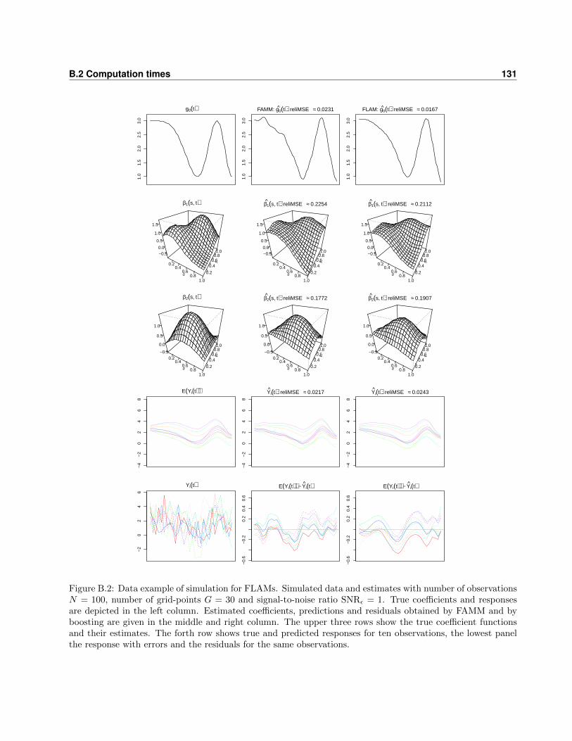
B.2 Computation times 131
1.0
1.5
2.0
2.5
3.0
g0(t)
1.0
1.5
2.0
2.5
3.0
FAMM: g0(t): reliMSE ≈ 0.0231
1.0
1.5
2.0
2.5
3.0
FLAM: g0(t): reliMSE ≈ 0.0167
s
0.20.4
0.60.8
1.0
t
0.2
0.40.60.81.0−0.5
0.0
0.5
1.0
1.5
β1(s, t)
s
0.20.4
0.60.8
1.0
t
0.2
0.40.60.81.0−0.5
0.0
0.5
1.0
1.5
β1^ (s, t): reliMSE ≈ 0.2254
s
0.20.4
0.60.8
1.0
t
0.2
0.40.60.81.0−0.5
0.0
0.5
1.0
1.5
β1^ (s, t): reliMSE ≈ 0.2112
s
0.20.4
0.60.8
1.0
t
0.2
0.40.60.81.0
−0.5
0.0
0.5
1.0
β2(s, t)
s
0.20.4
0.60.8
1.0
t
0.2
0.40.60.81.0
−0.5
0.0
0.5
1.0
β2^ (s, t): reliMSE ≈ 0.1772
s
0.20.4
0.60.8
1.0
t
0.2
0.40.60.81.0
−0.5
0.0
0.5
1.0
β2^ (s, t): reliMSE ≈ 0.1907
−4
−2
02
46
8
E(Yi(t))
−4
−2
02
46
8
Yi^ (t): reliMSE ≈ 0.0217
−4
−2
02
46
8
Yi^ (t): reliMSE ≈ 0.0243
−2
02
46
Yi(t)
−0.
6−
0.2
0.2
0.4
0.6
E(Yi(t)) − Yi^ (t)
−0.
6−
0.2
0.2
0.4
0.6
E(Yi(t)) − Yi^ (t)
Figure B.2: Data example of simulation for FLAMs. Simulated data and estimates with number of observationsN = 100, number of grid-points G = 30 and signal-to-noise ratio SNRε = 1. True coefficients and responsesare depicted in the left column. Estimated coefficients, predictions and residuals obtained by FAMM and byboosting are given in the middle and right column. The upper three rows show the true coefficient functionsand their estimates. The forth row shows true and predicted responses for ten observations, the lowest panelthe response with errors and the residuals for the same observations.
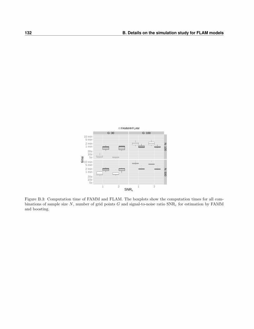
132 B. Details on the simulation study for FLAM models
G: 30 G: 100
●
●
●●●
●
●
●
●
●●
5s10s20s
1 min2 min5 min
10 min
5s10s20s
1 min2 min5 min
10 min
N: 100
N: 500
1 2 1 2SNRε
time
FAMM FLAM
Figure B.3: Computation time of FAMM and FLAM. The boxplots show the computation times for all com-binations of sample size N , number of grid points G and signal-to-noise ratio SNRε for estimation by FAMMand boosting.

Appendix C
Details for simulation and application
of the models with historical effects
This part of the appendix is based on the web appendix of the following paper:
Brockhaus, S., Melcher, M., Leisch, F., and Greven, S. (2016): Boosting flexible func-
tional regression models with a high number of functional historical effects. Statistics and
Computing, accepted, DOI: http://dx.doi.org/10.1007/s11222-016-9662-1.
C.1 Data generation in the simulation study
Generation of random coefficient functions. We generate the random coefficient functions βj(s, t) as
linear combinations of cubic P-splines (Eilers and Marx, 1996) with random coefficients. As penalty
first or second order difference matrices are used, dβ ∈ {1, 2}. In detail the coefficient functions are
generated by βj(s, t) = I(s ≤ t)BjΘjB>Y , j = 1, 2. Each design matrix Bj and BY contains basis
evaluations of five cubic B-splines. The random coefficients Θj are drawn from a normal distribution,
vec(Θj) ∼ N(0, (0.1I + P jY )−1
). The penalty matrix P jY is defined as in equation (4.4), where
λj = λY = 1 and the marginal penalty matrices P j , P Y are squared difference matrices of first or
second order, dβ ∈ {1, 2}.
Simulation settings. For the simulated functional covariates, Figure C.1 shows ten simulated
observations per data generating process. As an example for the random coefficients and the
resulting response variables, Figure C.2 presents the true and estimated coefficients for a random
iteration with data generating process bsplines-5 and Figure C.3 for lines-0. The random coefficient
surfaces are generated using first order difference penalties (dβ = 1). The estimation is conducted by
FAMM (center column) and boosting (right column) using a difference penalty of first order (ps-1).
All coefficient estimates are of the right magnitude and are similar in shape to the true surfaces.
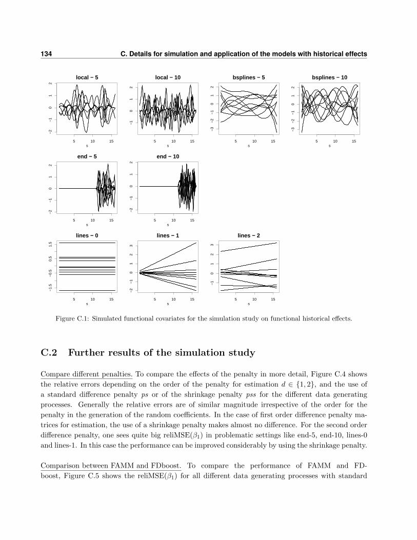
134 C. Details for simulation and application of the models with historical effects
5 10 15
−2
−1
01
2
local − 5
s5 10 15
−1
01
2
local − 10
s5 10 15
−3
−2
−1
01
2
bsplines − 5
s5 10 15
−3
−2
−1
01
2
bsplines − 10
s
5 10 15
−2
−1
01
2
end − 5
s5 10 15
−2
−1
01
2
end − 10
s
5 10 15
−1.
5−
0.5
0.5
1.5
lines − 0
s5 10 15
−2
−1
01
23
lines − 1
s5 10 15
−1
01
23
lines − 2
s
Figure C.1: Simulated functional covariates for the simulation study on functional historical effects.
C.2 Further results of the simulation study
Compare different penalties. To compare the effects of the penalty in more detail, Figure C.4 shows
the relative errors depending on the order of the penalty for estimation d ∈ {1, 2}, and the use of
a standard difference penalty ps or of the shrinkage penalty pss for the different data generating
processes. Generally the relative errors are of similar magnitude irrespective of the order for the
penalty in the generation of the random coefficients. In the case of first order difference penalty ma-
trices for estimation, the use of a shrinkage penalty makes almost no difference. For the second order
difference penalty, one sees quite big reliMSE(β1) in problematic settings like end-5, end-10, lines-0
and lines-1. In this case the performance can be improved considerably by using the shrinkage penalty.
Comparison between FAMM and FDboost. To compare the performance of FAMM and FD-
boost, Figure C.5 shows the reliMSE(β1) for all different data generating processes with standard
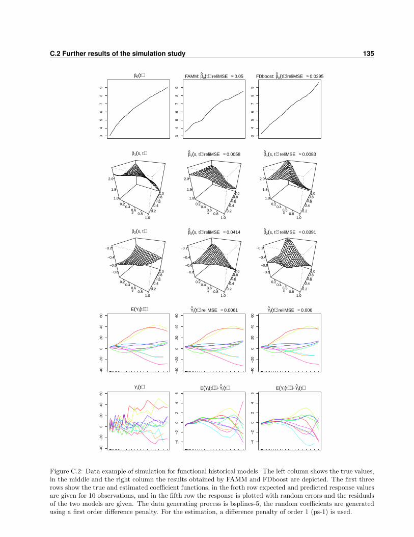
C.2 Further results of the simulation study 135
34
56
78
9
β0(t)
34
56
78
9
FAMM: β0(t): reliMSE ≈ 0.05
34
56
78
9
FDboost: β0(t): reliMSE ≈ 0.0295
s
0.20.4
0.60.8
1.0
t
0.2
0.40.60.81.0
1.0
1.5
2.0
β1(s, t)
s
0.20.4
0.60.8
1.0
t
0.2
0.40.60.81.0
1.0
1.5
2.0
β1(s, t): reliMSE ≈ 0.0058
s
0.20.4
0.60.8
1.0
t
0.2
0.40.60.81.0
1.0
1.5
2.0
β1(s, t): reliMSE ≈ 0.0083
s
0.20.4
0.60.8
1.0
t
0.2
0.40.60.81.0−0.8
−0.6
−0.4
−0.2
β2(s, t)
s
0.20.4
0.60.8
1.0
t
0.2
0.40.60.81.0−0.8
−0.6
−0.4
−0.2
β2(s, t): reliMSE ≈ 0.0414
s
0.20.4
0.60.8
1.0
t
0.2
0.40.60.81.0−0.8
−0.6
−0.4
−0.2
β2(s, t): reliMSE ≈ 0.0391
−40
−20
020
4060
E(Yi(t))
●●●●●●
●●●
●●
●●
●●
● ● ● ● ● ● ●
●●●●●●●● ●●●● ● ● ● ● ● ●● ● ● ● ●
●●●●●● ●●●●●
●●
●●
●●
●●
● ●●
●●●●●●
●●● ● ● ● ● ● ● ● ●●
●
●●
●●●●●●●●●●●● ● ● ● ● ● ● ● ● ● ●●
●●
●
●●●●●●●● ●● ● ● ● ● ● ● ●●
● ● ●
●●●●●●●●●●●●● ● ● ● ● ● ● ● ●●●●●●●●●● ●● ● ● ● ● ● ● ●
● ● ● ●
●●●●●●●●●●●● ● ● ● ● ● ● ●●
●●
●
●●●●●●● ●●●● ●
●●
●●
●
●●
●●
−40
−20
020
4060
Yi(t): reliMSE ≈ 0.0061
●●●●●●
●●●
●●
●●
●●
● ● ● ● ● ● ●
●●●●●●●● ●●●● ● ● ● ● ● ●● ● ● ● ●
●●●●●● ●●●●●
●●
●●
●●
●●
● ●●
●●●●●●
●●● ● ● ● ● ● ● ● ● ● ●
●●
●●●●●●●●●●●● ● ● ● ● ● ● ● ● ● ●●
●●
●
●●●●●●●● ●● ● ● ● ● ● ● ●●
● ● ●
●●●●●●●●●●●●● ● ● ● ● ● ● ● ●
●●●●●●●●● ●● ● ● ● ● ● ● ● ● ● ● ●
●●●●●●●●●●●● ● ● ● ● ● ● ●●
●●
●
●●●●●●● ●●●● ●
●●
●●
●
●● ● ●
−40
−20
020
4060
Yi(t): reliMSE ≈ 0.006
−40
−20
020
4060
Yi(t)
−4
−2
02
46
E(Yi(t)) − Yi(t)
−4
−2
02
46
E(Yi(t)) − Yi(t)
Figure C.2: Data example of simulation for functional historical models. The left column shows the true values,in the middle and the right column the results obtained by FAMM and FDboost are depicted. The first threerows show the true and estimated coefficient functions, in the forth row expected and predicted response valuesare given for 10 observations, and in the fifth row the response is plotted with random errors and the residualsof the two models are given. The data generating process is bsplines-5, the random coefficients are generatedusing a first order difference penalty. For the estimation, a difference penalty of order 1 (ps-1) is used.
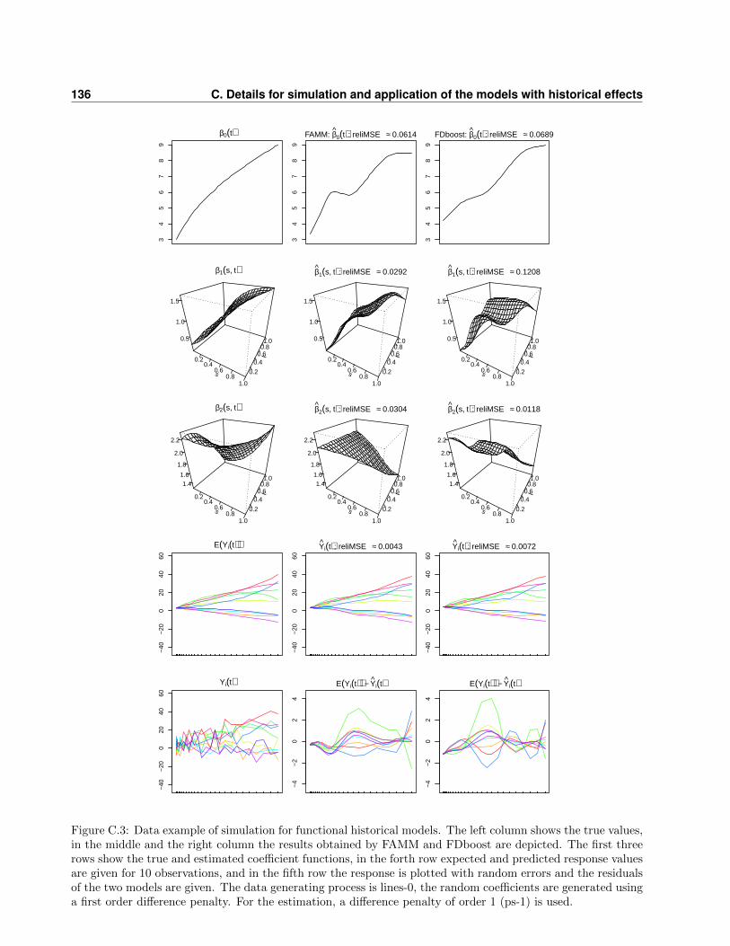
136 C. Details for simulation and application of the models with historical effects
34
56
78
9
β0(t)
34
56
78
9
FAMM: β0(t): reliMSE ≈ 0.0614
34
56
78
9
FDboost: β0(t): reliMSE ≈ 0.0689
s
0.20.4
0.60.8
1.0
t
0.2
0.40.60.81.00.5
1.0
1.5
β1(s, t)
s
0.20.4
0.60.8
1.0
t
0.2
0.40.60.81.00.5
1.0
1.5
β1(s, t): reliMSE ≈ 0.0292
s
0.20.4
0.60.8
1.0
t
0.2
0.40.60.81.00.5
1.0
1.5
β1(s, t): reliMSE ≈ 0.1208
s
0.20.4
0.60.8
1.0
t
0.2
0.40.60.81.0
1.41.6
1.8
2.0
2.2
β2(s, t)
s
0.20.4
0.60.8
1.0
t
0.2
0.40.60.81.0
1.41.6
1.8
2.0
2.2
β2(s, t): reliMSE ≈ 0.0304
s
0.20.4
0.60.8
1.0
t
0.2
0.40.60.81.0
1.41.6
1.8
2.0
2.2
β2(s, t): reliMSE ≈ 0.0118
−40
−20
020
4060
E(Yi(t))
●●●●●●● ● ●● ●● ● ● ● ●
●
●●
●●●● ●●● ● ● ● ● ● ● ● ● ● ● ●
●●●●●●●● ●●● ● ● ● ● ● ● ● ● ● ● ● ● ● ●
●●●●●●●●●
●● ● ● ● ● ● ● ● ● ● ●
●●●●●●●●●● ● ● ● ● ● ● ● ● ● ● ● ●
●●●●●●●●●●●● ● ● ● ● ● ● ● ● ●
●●●● ●●●●●● ● ● ● ●● ● ●
●
●●
●
●●●●●● ●●● ● ● ● ● ● ● ● ● ● ● ● ●
●●● ●●● ●● ● ●● ● ● ● ● ● ●
●
●●●●●●●●●●●●● ● ● ● ● ● ● ●●
● ● ●
−40
−20
020
4060
Yi(t): reliMSE ≈ 0.0043
●●●●●●● ● ●● ●● ● ● ● ●
●
● ●
●●●● ●●● ● ● ● ● ● ● ● ● ● ● ●
●●●●●●●● ●●● ● ● ● ● ● ● ● ● ● ● ● ● ● ●
●●●●●●●●●
●● ● ● ● ●●
● ●●
● ●
●●●●●● ●●●● ● ● ● ●● ● ● ● ● ● ● ●
●●●●●●●●●●●● ● ● ● ● ● ● ● ● ●
●●●● ●●●●●● ●● ● ● ● ● ●
●
●● ●
●●●●●● ●●● ● ● ● ● ● ● ● ● ● ● ● ●
●●● ●●● ●● ● ●● ● ● ● ● ● ●
●
●●●●●●●●●●●●● ● ● ● ● ● ●●
●● ● ●
−40
−20
020
4060
Yi(t): reliMSE ≈ 0.0072
−40
−20
020
4060
Yi(t)
−4
−2
02
4
E(Yi(t)) − Yi(t)
−4
−2
02
4
E(Yi(t)) − Yi(t)
Figure C.3: Data example of simulation for functional historical models. The left column shows the true values,in the middle and the right column the results obtained by FAMM and FDboost are depicted. The first threerows show the true and estimated coefficient functions, in the forth row expected and predicted response valuesare given for 10 observations, and in the fifth row the response is plotted with random errors and the residualsof the two models are given. The data generating process is lines-0, the random coefficients are generated usinga first order difference penalty. For the estimation, a difference penalty of order 1 (ps-1) is used.

C.2 Further results of the simulation study 137
●
●
●
●
● ●
●●
●
●
●
●
●
●
●
●
●
●
●
●
●
●
●●
●
●
●
●
●
●●
●
●
●
●
●
●
●
●
●
●●
●
●●
●
●
●●
●
●
●
●
ps−1 ps−2
pss−1 pss−2
1e−02
1e+00
1e+02
1e−02
1e+00
1e+02
1 2 1 2dβ
reliM
SE
(β1) local−5
local−10bsplines−5bsplines−10end−5end−10lines−0lines−1lines−2
Figure C.4: Simulation results comparing different penalties. The reliMSE(β1) for different penalties in theestimation are given in the panels. The partition is as follows: on the left first order difference penalty d = 1,on the right second order difference penalty d = 2, upper panel difference penalty ps and lower panel shrinkagepenalty pss. On the x-axis the order of the penalty for the generation of the random coefficients is given fordβ ∈ {1, 2}. Results are shown for estimation by boosting on a logarithmic scale.
first order difference penalties (ps-1). There are big differences between the data settings. For
covariates that are generated using B-splines over the whole domain, for local data settings and
for lines-2, the relative estimation errors are mostly under 0.1 indicating good estimation of the
coefficient surfaces. For the other settings, with covariates containing less information, the coefficients
are fitted more accurately if the penalty used for the generation of the random coefficient and for
fitting are of the same order. This effect is most pronounced for the end settings. Apart from the
end settings most relative errors are below one. The performance of FAMM and FDboost is similar,
although FDboost outperforms FAMM for the settings lines-0 and lines-1 with dβ = 2. When adding
8 nuisance variables FAMM is no longer able to fit the models. Using boosting, the models can
be fitted without problems using all covariates and the relative errors for the influential variables
increase only slightly, see the bottom row of Figure C.5. When just fitting the models by boosting,
usually some of the nuisance variables enter the models with small coefficient effects.
To check in addition the ability of stability selection to select the influential variables, we use in
a second step stability selection on the settings with nuisance variables. We use 50 complementary
pairs, a threshold of πthr = 0.9 and PFER < 0.1 · J = 1.1 for J = 11 base-learners, inducing q = 5
(see Section 4.4 for an introduction to stability selection). The two influential variables are always
selected, and only rarely is a non-influential variable selected as third variable. Thus, the estimation
errors in the models with stability selection remain almost the same as for the settings without
nuisance variables and are not shown here.
Computation time. In Figure C.6 the computation times of the model fits on a 64-bit linux
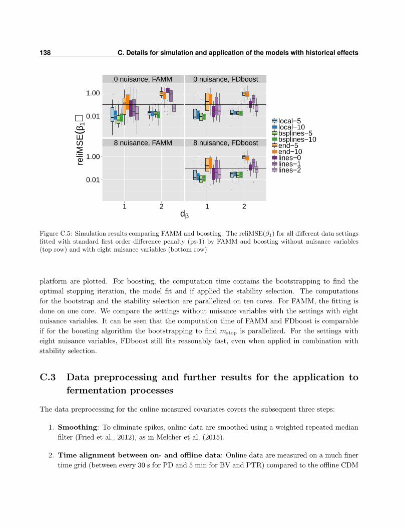
138 C. Details for simulation and application of the models with historical effects
●
●
●
●
●●
●●
● ●
●
●
●
●
●
●
●
●●
●
●
●
●
●
●
●
●
●
●
● ●
●
●
●
●
●
●
●
●
●
0 nuisance, FAMM 0 nuisance, FDboost
8 nuisance, FAMM 8 nuisance, FDboost
0.01
1.00
0.01
1.00
1 2 1 2dβ
reliM
SE
(β1) local−5
local−10bsplines−5bsplines−10end−5end−10lines−0lines−1lines−2
Figure C.5: Simulation results comparing FAMM and boosting. The reliMSE(β1) for all different data settingsfitted with standard first order difference penalty (ps-1) by FAMM and boosting without nuisance variables(top row) and with eight nuisance variables (bottom row).
platform are plotted. For boosting, the computation time contains the bootstrapping to find the
optimal stopping iteration, the model fit and if applied the stability selection. The computations
for the bootstrap and the stability selection are parallelized on ten cores. For FAMM, the fitting is
done on one core. We compare the settings without nuisance variables with the settings with eight
nuisance variables. It can be seen that the computation time of FAMM and FDboost is comparable
if for the boosting algorithm the bootstrapping to find mstop is parallelized. For the settings with
eight nuisance variables, FDboost still fits reasonably fast, even when applied in combination with
stability selection.
C.3 Data preprocessing and further results for the application to
fermentation processes
The data preprocessing for the online measured covariates covers the subsequent three steps:
1. Smoothing: To eliminate spikes, online data are smoothed using a weighted repeated median
filter (Fried et al., 2012), as in Melcher et al. (2015).
2. Time alignment between on- and offline data: Online data are measured on a much finer
time grid (between every 30 s for PD and 5 min for BV and PTR) compared to the offline CDM
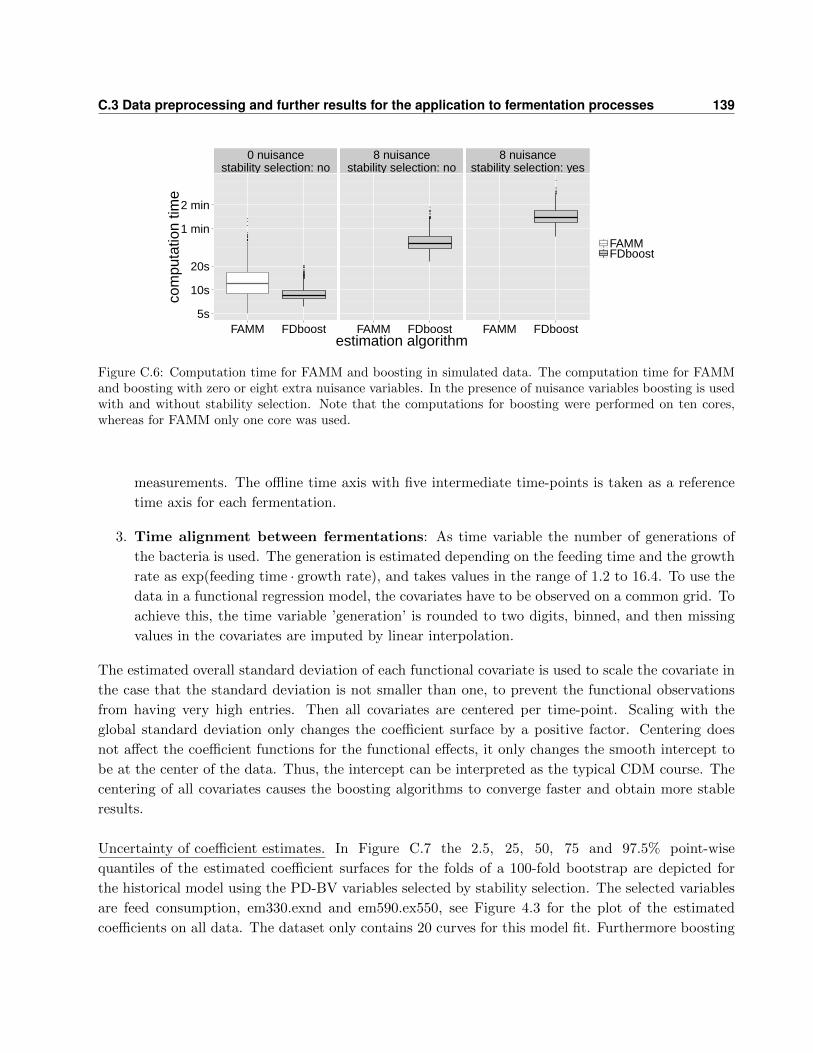
C.3 Data preprocessing and further results for the application to fermentation processes 139
0 nuisancestability selection: no
8 nuisancestability selection: no
8 nuisancestability selection: yes
●
●
●
●
●●●●
●
●●●
●
●
●●
●
●
●
●
●
●
●
●
●
●
●
●
●●
●
●
●
●
●
●
●
●●
●
●●
●
●
●
●
●
●
●
●
●
●
●
●
●●
●
●
●
●
●●
●●
●
●
●
●
●
●
●
●
●
●
●
●●●●
●
●●
●
●
●
●●●
●
●●
●
●
●
●
●●
●
●●
●
●
5s
10s
20s
1 min
2 min
FAMM FDboost FAMM FDboost FAMM FDboostestimation algorithm
com
puta
tion
time
FAMMFDboost
Figure C.6: Computation time for FAMM and boosting in simulated data. The computation time for FAMMand boosting with zero or eight extra nuisance variables. In the presence of nuisance variables boosting is usedwith and without stability selection. Note that the computations for boosting were performed on ten cores,whereas for FAMM only one core was used.
measurements. The offline time axis with five intermediate time-points is taken as a reference
time axis for each fermentation.
3. Time alignment between fermentations: As time variable the number of generations of
the bacteria is used. The generation is estimated depending on the feeding time and the growth
rate as exp(feeding time · growth rate), and takes values in the range of 1.2 to 16.4. To use the
data in a functional regression model, the covariates have to be observed on a common grid. To
achieve this, the time variable ’generation’ is rounded to two digits, binned, and then missing
values in the covariates are imputed by linear interpolation.
The estimated overall standard deviation of each functional covariate is used to scale the covariate in
the case that the standard deviation is not smaller than one, to prevent the functional observations
from having very high entries. Then all covariates are centered per time-point. Scaling with the
global standard deviation only changes the coefficient surface by a positive factor. Centering does
not affect the coefficient functions for the functional effects, it only changes the smooth intercept to
be at the center of the data. Thus, the intercept can be interpreted as the typical CDM course. The
centering of all covariates causes the boosting algorithms to converge faster and obtain more stable
results.
Uncertainty of coefficient estimates. In Figure C.7 the 2.5, 25, 50, 75 and 97.5% point-wise
quantiles of the estimated coefficient surfaces for the folds of a 100-fold bootstrap are depicted for
the historical model using the PD-BV variables selected by stability selection. The selected variables
are feed consumption, em330.exnd and em590.ex550, see Figure 4.3 for the plot of the estimated
coefficients on all data. The dataset only contains 20 curves for this model fit. Furthermore boosting

140 C. Details for simulation and application of the models with historical effects
Table C.1: Results of stability selection for functional historical models. The first 20 variables in the order asselected by stability selection using the historical model for the three different sets of covariates. The percentageof selection among the first q variables is given in parentheses. For the PTR variables, ’r’ means the rate ofthe substance and ’c’ the cumulative amount.
PD (πj) PD-BV (πj) PD-PTR (πj)
base consumption (81) em590.ex550 (99) dissolved O2 (88)head pressure (74) intercept (97) indole r (86)dissolved O2 (62) em330.exnd (92) acetaldehyde c (80)
air flow (41) feed consumption (90) CO2 in exhaust gas (76)CO2 in exhaust gas (21) dissolved O2 (89) methanthiole r (73)
feed consumption (9) head pressure (87) acetaldehyde r (68)intercept (6) em530.ex430 (84) dimethyldisulfide r (67)
O2 in exhaust gas (6) em590.ex270 (81) butanone or 3-Buten-1ol c1 (66)CO2 in exhaust gas (80) feed consumption (65)
O2 in exhaust gas (74) head pressure (62)base consumption (74) indole c (59)
em350.ex310 (69) methanthiole c (57)em450.ex410 (68) base consumption (56)
air flow (65) intercept (54)em410.ex330 (65) butanol c (50)em390.ex350 (64) isoprene c (44)em490.ex290 (63) dimethyldisulfide c (42)em410.ex350 (59) isoprene r (41)em430.ex390 (59) ethanol c (38)em590.ex290 (58) butanol r (37)emnd.ex270 (50) butanone or 3-Buten-1ol r1 (33)
1 For mass M = 73, the substances butanone and 3-Buten-1ol are possible.
induces shrinkage of the coefficients and thus the plotted quantiles can only by interpreted as a
measure of uncertainty for the estimated coefficients, not as point-wise confidence intervals. For feed
consumption, the estimated surfaces greatly differ over the folds and the point-wise median is zero.
For the spectroscopic variables em330.exnd and em590.ex550, the coefficient surfaces are estimated
more consistently over the folds, showing similar structures at the plotted quantiles.

C.3 Data preprocessing and further results for the application to fermentation processes 141
feed consumption, at 2.5%
generation
gene
ratio
n_s
−240
−200
−18
0
−140
−120
−10
0
−60
−60
−40
5 10 15
510
15
em330.exnd, at 2.5%
generation
gene
ratio
n_s
−16
−12 −10 −8
−8
−6 −4
−4
−2 0
0
2
2
5 10 15
510
15
em590.ex550, at 2.5%
generation
gene
ratio
n_s −18 −
16
−14
−14
−12
−12
−10
−8
−6 −6
5 10 15
510
15
feed consumption, at 25%
generation
gene
ratio
n_s
−12
−10 −8
−6
−4
−4
−2
−2
−2
0
5 10 15
510
15
em330.exnd, at 25%
generation
gene
ratio
n_s
−8 −6 −4
−4
−2 0
0
2
2
4
4
6
5 10 15
510
15
em590.ex550, at 25%
generation
gene
ratio
n_s
−6.
5
−6.5 −6 −5.5
−5
−4.5
−4
−3.
5
−3
−2.5
−2
−1.5
5 10 15
510
15
feed consumption, at 50%
generation
gene
ratio
n_s
5 10 15
510
15
em330.exnd, at 50%
generation
gene
ratio
n_s
−4 −2
−2
0
2
2
4
4
6
6
8
5 10 15
510
15
em590.ex550, at 50%
generation
gene
ratio
n_s
−3.5
−3
−3
−2.5 −2
−1.
5
−1
−0.5
0
0.5
1
1.5
2
2.5
5 10 15
510
15
feed consumption, at 75%
generation
gene
ratio
n_s
5 10 15
510
15
em330.exnd, at 75%
generation
gene
ratio
n_s
−1 0 1
1
2 3 4
5
5
6
6
7 8
9
5 10 15
510
15
em590.ex550, at 75%
generation
gene
ratio
n_s
−1
−1
0
1 2
3
4
5
6
7
8
5 10 15
510
15
feed consumption, at 97.5%
generation
gene
ratio
n_s
10
20
30
30
40 50
60
70
80 90
100
120
5 10 15
510
15
em330.exnd, at 97.5%
generation
gene
ratio
n_s
3 4
5
6 7 8
8
9
10
10
11
12
12 13
5 10 15
510
15
em590.ex550, at 97.5%
generation
gene
ratio
n_s
2
4
6
8
10 12
14
16
20 22
24
5 10 15
510
15
Figure C.7: Bootstrapped coefficient estimates. The 2.5, 25, 50, 75 and 97.5% point-wise quantiles of theestimated coefficient surfaces for the folds of a 100-fold bootstrap (rows from top to bottom) are depicted forthe historical model using feed consumption, em330.exnd and em590.ex550 as covariates (columns from left toright). Red means positive, blue negative and gray zero effects.

142 C. Details for simulation and application of the models with historical effects
Table C.2: Identifiability measures for the selected variables. As identifiability measures the common logarithmof the condition number log10 κj and the maximal null space overlap maxtg
⋂Xj⊥P⊥
(tg) are given for the threeselected functional covariates.
covariate log10 κj maxtg⋂Xj⊥P⊥(tg)
em590.ex550 8.56 0.10em330.exnd 6.24 0.11feed consumption 8.58 0.11
Appendix D
Implementation of signal GAMLSS
and further details on application and
simulation
This part of the appendix is based on the appendix of the following paper:
Brockhaus, S., Fuest, A., Mayr, A. and Greven, S. (2016): Signal regression mod-
els for location, scale and shape with an application to stock returns. arXiv preprint,
arXiv:1605.04281.
D.1 Details on the implementation of the estimation methods
D.1.1 Used R packages
All computations are performed using R software for statistical computing (R Core Team, 2015).
Boosting for GAMLSS, Section 5.4, is implemented in the R package gamboostLSS (Hofner et al.,
2015b) and base-learners for functional covariates are available in the FDboost package (Brockhaus
and Rugamer, 2016). The gamboostLSS package provides the possibility to use all distribution families
implemented in the gamlss-package (Stasinopoulos et al., 2016).
Estimation of GAMLSS by maximizing the penalized log-likelihood using backfitting, Sec-
tion 5.5.1, is implemented in the R package gamlss (Stasinopoulos et al., 2016). The linear func-
tional effect and many other additive effects are available using the R package gamlss.add (Rigby and
Stasinopoulos, 2015) to incorporate additive effects of the R package mgcv (Wood, 2016) into the
GAMLSS models.
Estimation of GAMLSS by maximizing the penalized log-likelihood using LAML, Section 5.5.2,
is implemented in the R package mgcv (Wood, 2016), which contains linear functional effects and has
many additive terms implemented. Note that in R package mgcv the Gaussian location scale family
models the inverse standard deviation instead of the standard deviation.

144 D. Implementation of signal GAMLSS and further details on application and simulation
To incorporate functional effects with FPC-basis expansion, any software can be used to estimate
the FPCA. The scores can then be used like scalar covariates in the models. We use the R package
refund (Huang et al., 2016) for the estimation of the FPCA.
D.1.2 Example R code
The application of the three estimation methods–boosting, gamlss and mgcv–in R is demonstrated
on a small simulated example for a Gaussian location scale model with a linear effect of one scalar
and one functional covariate:
########### simulate Gaussian data
library(splines)
n <- 500 ## number of observations
G <- 120 ## number of evaluation points per functional covariate
set.seed(123) ## ensure reproducibility
z <- runif(n) ## scalar covariate
z <- z - mean(z)
s <- seq(0, 1, l = G) ## index of functional covariate
## generate functional covariate
x <- t(replicate(n, drop(bs(s, df = 5, int = TRUE) %*%
runif(5, min = -1, max = 1))))
## center x per observation point
x <- scale(x, center = TRUE, scale = FALSE)
mu <- 2 + 0.5*z + (1/G*x) %*% sin(s*pi)*5 ## true functions for expectation
sigma <- exp(0.5*z - (1/G*x) %*% cos(s*pi)*2) ## and for standard deviation
y <- rnorm(mean = mu, sd = sigma, n = n) ## draw respone y_i ~ N(mu_i, sigma_i)
########### fit by boosting
library(gamboostLSS)
library(FDboost)
## save data as list containing s as well
dat_list <- list(y = y, z = z, x = I(x), s = s)
## model fit by boosting
## bols: linear base-learner for scalar covariates
## bsignal: linear base-learner for functional covariates
m_boost <- FDboostLSS(list(mu = y ~ bols(z, df = 2) +
bsignal(x, s, df = 2, knots = 16),
sigma = y ~ bols(z, df = 2) +
bsignal(x, s, df = 2, knots = 16)),
timeformula = NULL, data = dat_list)
## find optimal number of boosting iterations on a 2D grid in [1, 500]
## using 5-fold bootstrap
grid <- make.grid(c(mu = 500, sigma = 500), length.out = 10)
## takes some time, easy to parallelize on Linux

D.1 Details on the implementation of the estimation methods 145
cvr <- cvrisk(m_boost, folds = cv(model.weights(m_boost), B = 5),
grid = grid, trace = FALSE)
## use model at optimal stopping iterations
m_boost <- m_boost[mstop(cvr)] ## m_boost[c(253, 126)]
summary(m_boost)
## plot smooth effects of functional covariates
par(mfrow = c(1,2))
plot(m_boost$mu, which = 2, ylim = c(0,5))
lines(s, sin(s*pi)*5, col = 3, lwd = 2)
plot(m_boost$sigma, which = 2, ylim = c(-2.5,2.5))
lines(s, -cos(s*pi)*2, col=3, lwd = 2)
## do a QQ-plot of the quantile residuals
## compute quantile residuals
predmui <- predict(m_boost, parameter = "mu", type = "response")
predsigmai <- predict(m_boost, parameter = "sigma", type = "response")
yi <- m_boost$mu$response
resi_boosting <- (yi - predmui) / predsigmai
#### alternative way to compute the quantile residuals,
#### which also works for non-Gaussian responses
## library(gamlss)
## resi_boosting <- qnorm(pNO(q = yi, mu = predmui, sigma = predsigmai))
qqnorm(resi_boosting, main = "", ylim = c(-4, 4), xlim = c(-4, 4))
abline(0, 1, col = "darkgrey", lwd = 0.6, cex = 0.5)
########### fit by gamlss
library(mgcv)
library(gamlss)
library(gamlss.add)
## multiply functional covariate with integration weights
xInt <- 1/G * x
## sma: matrix containing the evaluation points s in each row
dat <- data.frame(y = y, z = z, x = I(xInt),
sma = I(t(matrix(s, length(s), n))))
## model fit by gamlss
## use ga() from gamlss.add to incorporate smooth effects from mgcv
m_gamlss <- gamlss(y ~ z +
ga( ~ s(sma, by = x, bs = "ps", m = c(2, 1), k = 20)),
sigma.formula = ~ z +
ga( ~ s(sma, by = x, bs = "ps", m = c(2, 1), k = 20)),
data = dat)
summary(m_gamlss)
## plot smooth effects of functional covariates
plot(getSmo(m_gamlss, what = "mu"))
lines(s, sin(s*pi)*5, col = 3, lwd = 2)

146 D. Implementation of signal GAMLSS and further details on application and simulation
plot(getSmo(m_gamlss, what = "sigma"))
lines(s, -cos(s*pi)*2, col = 3, lwd = 2)
########### fit by mgcv
library(mgcv)
## multiply functional covariate with integration weights
xInt <- 1/G * x
## sma: matrix containing the evaluation points s in each row
dat <- data.frame(y = y, z = z, x = I(xInt),
sma = I(t(matrix(s, length(s), n))))
## model fit by mgcv
## note that gaulss in mgcv models the inverse standard deviation
m_mgcv <- gam(list(y ~ z +
s(sma, by = x, bs = "ps", m = c(2, 1), k = 20),
~ z +
s(sma, by = x, bs = "ps", m = c(2, 1), k = 20)),
data = dat, family = gaulss)
summary(m_mgcv)
## plot smooth effects of functional covariates
plot(m_mgcv, select = 1)
lines(s, sin(s*pi)*5, col = 3, lwd = 2)
plot(m_mgcv, select = 2)
lines(s, -cos(s*pi)*2, col = 3, lwd = 2)
########### fit with FPC-basis for the example of mgcv
library(refund)
## do the FPCA on x; explain 99% of variability
kl_x <- fpca.sc(x, pve = 0.99, argvals = s)
## scores that can be used like scalar covariates
scores <- kl_x$scores
dat <- data.frame(y = y, z = z, scores = scores)
## model fit by mgcv
m_mgcv_fpca <- gam(list(y ~ z + scores,
~ z + scores),
data = dat, family = gaulss)
summary(m_mgcv_fpca)
## plot smooth effects of functional covariates
coefs_scores <- coef(m_mgcv_fpca)[
grepl("scores", names(coef(m_mgcv_fpca)))]
coefs_scores_mu <- coefs_scores[1:kl_x$npc]
coefs_scores_sigma <- coefs_scores[(kl_x$npc+1):length(coefs_scores)]

D.2 Further results of the application on stock returns 147
plot(s, kl_x$efunctions %*% coefs_scores_mu, type = "l")
lines(s, sin(s*pi)*5, col = 3, lwd = 2)
plot(s, kl_x$efunctions %*% coefs_scores_sigma, type = "l")
lines(s, -cos(s*pi)*2, col = 3, lwd = 2)
D.2 Further results of the application on stock returns
In Figure D.1 the estimated ACF is plotted for the squared residuals of models fitted by gamlss.
In Figure D.2 the estimates for the model assuming a normal location scale model are plotted for
sc
0 5 10 15 20 25
0.0
0.2
0.4
0.6
0.8
1.0
Lag
AC
F
0 5 10 15 20 25
0.0
0.2
0.4
0.6
0.8
1.0
Lag
AC
F
sc+fun
0 5 10 15 20 25
0.0
0.2
0.4
0.6
0.8
1.0
Lag
AC
F
0 5 10 15 20 25
0.0
0.2
0.4
0.6
0.8
1.0
Lag
AC
F
Figure D.1: Model choice for the application on stock returns. The estimated ACF of the squared quantileresiduals in the GAMLSS with scalar variables (sc, top row) or with scalar and functional variables (sc+fun,bottom row) assuming normally distributed response (left column) or Students t-distribution for the response(right column) for models estimated by the gamlss algorithm. The dashed blue line marks the limits forpoint-wise 95% tests for the ACF to be zero.
boosting, as in Figure 5.3, and for mgcv the estimates resulting from using the shrinkage-penalty of
Marra and Wood (2011) with Kj = 10 basis functions are given. In Figure D.3 the estimates for the
model assuming a normal location scale model are plotted for boosting and for mgcv using FPC basis
functions to represent both, the functional covariate and the functional coefficient. We use the first
three eigenfunctions as those explain more than 99% of the variability in the bid- and ask-curves. The
confidence intervals are computed conditional on the estimated eigendecomposition. In Figure D.4
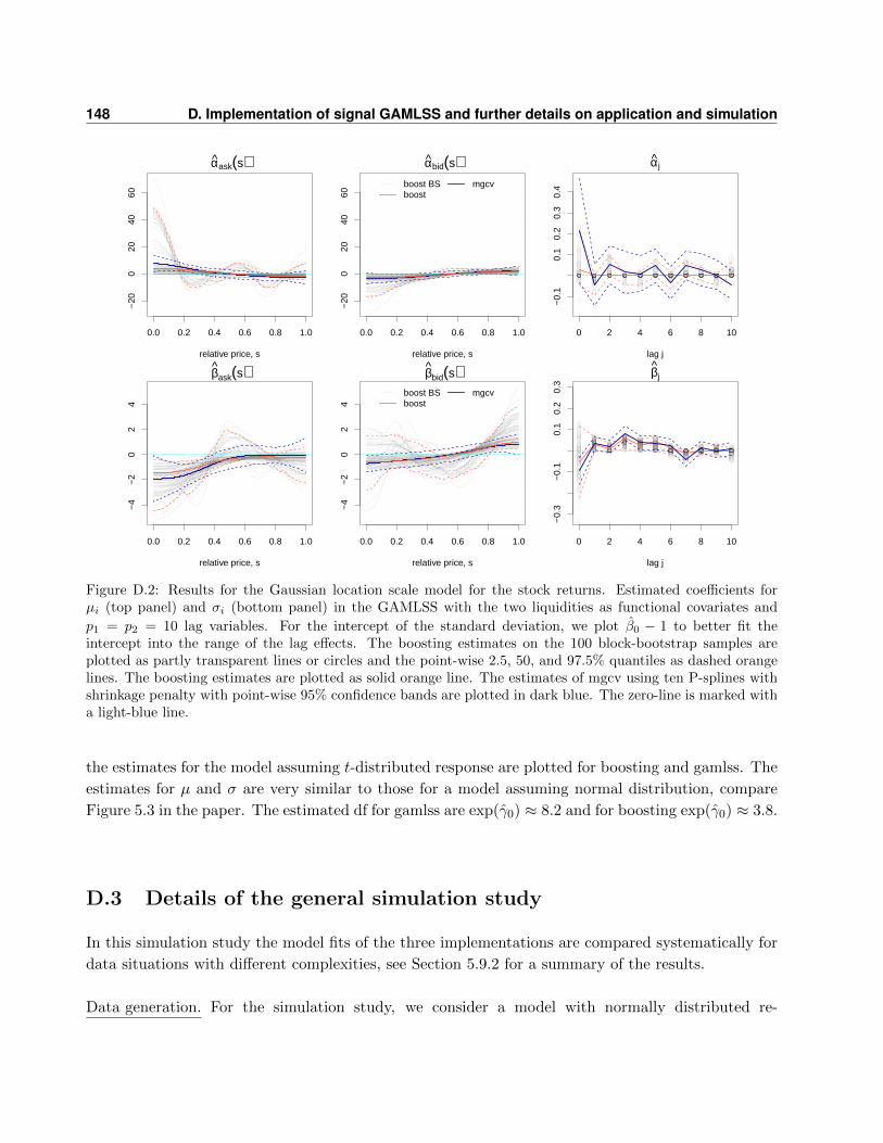
148 D. Implementation of signal GAMLSS and further details on application and simulation
0.0 0.2 0.4 0.6 0.8 1.0
−20
020
4060
αask(s)
relative price, s
0.0 0.2 0.4 0.6 0.8 1.0−
200
2040
60
αbid(s)
relative price, s
boost BSboost
mgcv
0 2 4 6 8 10
−0.
10.
10.
20.
30.
4
αj
lag j
0.0 0.2 0.4 0.6 0.8 1.0
−4
−2
02
4
βask(s)
relative price, s
0.0 0.2 0.4 0.6 0.8 1.0
−4
−2
02
4
βbid(s)
relative price, s
boost BSboost
mgcv
0 2 4 6 8 10
−0.
3−
0.1
0.1
0.2
0.3
βj
lag j
Figure D.2: Results for the Gaussian location scale model for the stock returns. Estimated coefficients forµi (top panel) and σi (bottom panel) in the GAMLSS with the two liquidities as functional covariates and
p1 = p2 = 10 lag variables. For the intercept of the standard deviation, we plot β0 − 1 to better fit theintercept into the range of the lag effects. The boosting estimates on the 100 block-bootstrap samples areplotted as partly transparent lines or circles and the point-wise 2.5, 50, and 97.5% quantiles as dashed orangelines. The boosting estimates are plotted as solid orange line. The estimates of mgcv using ten P-splines withshrinkage penalty with point-wise 95% confidence bands are plotted in dark blue. The zero-line is marked witha light-blue line.
the estimates for the model assuming t-distributed response are plotted for boosting and gamlss. The
estimates for µ and σ are very similar to those for a model assuming normal distribution, compare
Figure 5.3 in the paper. The estimated df for gamlss are exp(γ0) ≈ 8.2 and for boosting exp(γ0) ≈ 3.8.
D.3 Details of the general simulation study
In this simulation study the model fits of the three implementations are compared systematically for
data situations with different complexities, see Section 5.9.2 for a summary of the results.
Data generation. For the simulation study, we consider a model with normally distributed re-
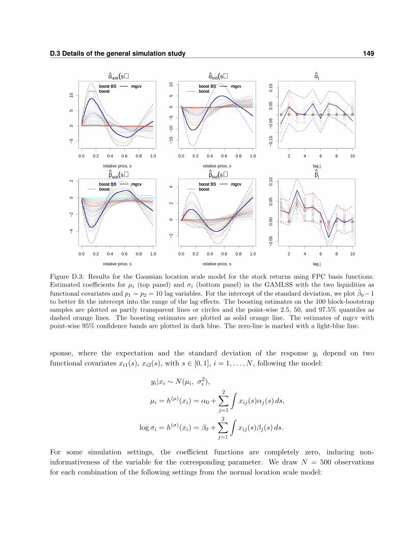
D.3 Details of the general simulation study 149
0.0 0.2 0.4 0.6 0.8 1.0
−5
05
10αask(s)
relative price, s
boost BSboost
mgcvboost BSboost
mgcv
0.0 0.2 0.4 0.6 0.8 1.0
−15
−10
−5
05
10
αbid(s)
relative price, s
boost BSboost
mgcvboost BSboost
mgcv
2 4 6 8 10
−0.
15−
0.05
0.05
0.15
αj
lag j
0.0 0.2 0.4 0.6 0.8 1.0
−4
−2
02
βask(s)
relative price, s
boost BSboost
mgcvboost BSboost
mgcv
0.0 0.2 0.4 0.6 0.8 1.0
−2
02
4βbid(s)
relative price, s
boost BSboost
mgcvboost BSboost
mgcv
2 4 6 8 10
−0.
050.
000.
050.
10
βj
lag j
Figure D.3: Results for the Gaussian location scale model for the stock returns using FPC basis functions.Estimated coefficients for µi (top panel) and σi (bottom panel) in the GAMLSS with the two liquidities as
functional covariates and p1 = p2 = 10 lag variables. For the intercept of the standard deviation, we plot β0−1to better fit the intercept into the range of the lag effects. The boosting estimates on the 100 block-bootstrapsamples are plotted as partly transparent lines or circles and the point-wise 2.5, 50, and 97.5% quantiles asdashed orange lines. The boosting estimates are plotted as solid orange line. The estimates of mgcv withpoint-wise 95% confidence bands are plotted in dark blue. The zero-line is marked with a light-blue line.
sponse, where the expectation and the standard deviation of the response yi depend on two
functional covariates xi1(s), xi2(s), with s ∈ [0, 1], i = 1, . . . , N , following the model:
yi|xi ∼ N(µi, σ2i ),
µi = h(µ)(xi) = α0 +
2∑j=1
∫xij(s)αj(s) ds,
log σi = h(σ)(xi) = β0 +
2∑j=1
∫xij(s)βj(s) ds.
For some simulation settings, the coefficient functions are completely zero, inducing non-
informativeness of the variable for the corresponding parameter. We draw N = 500 observations
for each combination of the following settings from the normal location scale model:
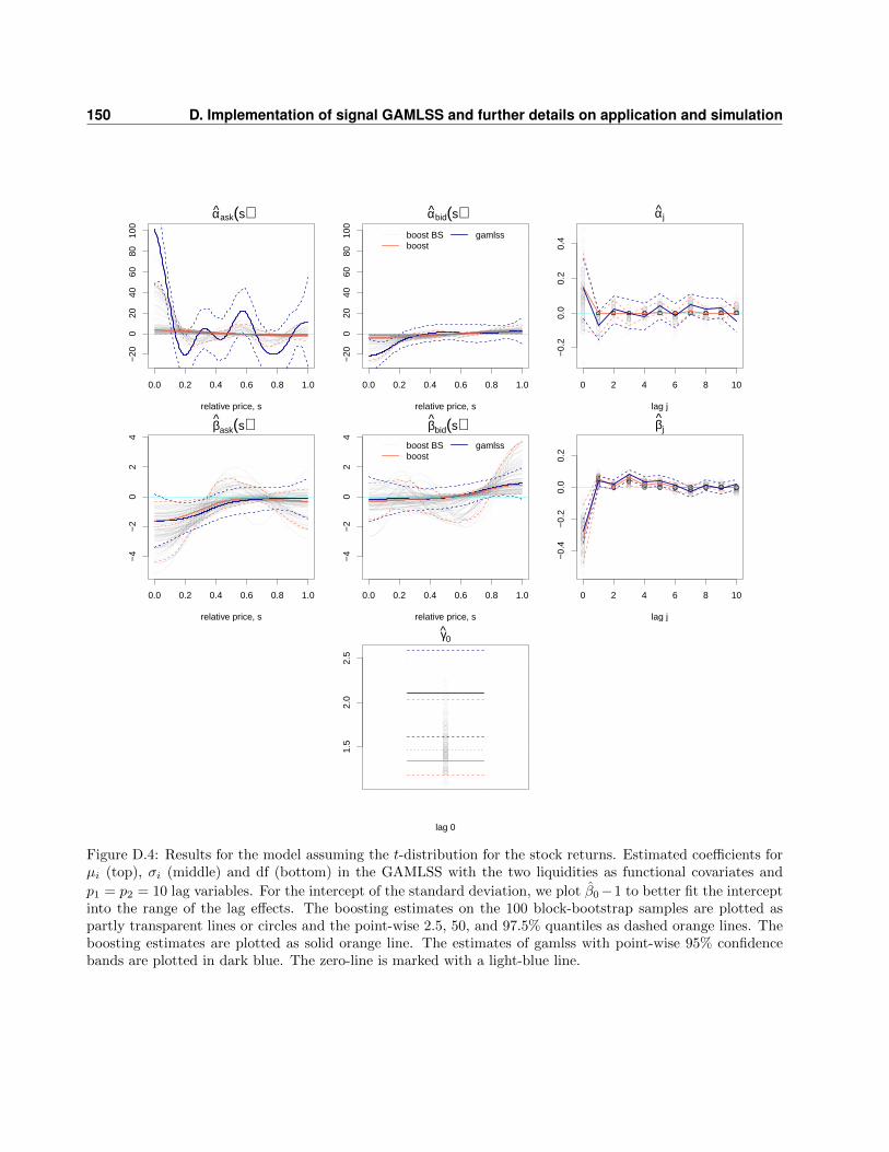
150 D. Implementation of signal GAMLSS and further details on application and simulation
0.0 0.2 0.4 0.6 0.8 1.0
−20
020
4060
8010
0
αask(s)
relative price, s
0.0 0.2 0.4 0.6 0.8 1.0
−20
020
4060
8010
0
αbid(s)
relative price, s
boost BSboost
gamlss
0 2 4 6 8 10
−0.
20.
00.
20.
4
αj
lag j
0.0 0.2 0.4 0.6 0.8 1.0
−4
−2
02
4
βask(s)
relative price, s
0.0 0.2 0.4 0.6 0.8 1.0
−4
−2
02
4
βbid(s)
relative price, s
boost BSboost
gamlss
0 2 4 6 8 10
−0.
4−
0.2
0.0
0.2
βj
lag j
1.5
2.0
2.5
γ0
lag 0
Figure D.4: Results for the model assuming the t-distribution for the stock returns. Estimated coefficients forµi (top), σi (middle) and df (bottom) in the GAMLSS with the two liquidities as functional covariates and
p1 = p2 = 10 lag variables. For the intercept of the standard deviation, we plot β0−1 to better fit the interceptinto the range of the lag effects. The boosting estimates on the 100 block-bootstrap samples are plotted aspartly transparent lines or circles and the point-wise 2.5, 50, and 97.5% quantiles as dashed orange lines. Theboosting estimates are plotted as solid orange line. The estimates of gamlss with point-wise 95% confidencebands are plotted in dark blue. The zero-line is marked with a light-blue line.

D.3 Details of the general simulation study 151
1. Simulate functional covariates xj(s), with 100 equally spaced evaluation points (s1, . . . , s100)>,
using C = 5 basis functions φc(s) =√
2 sin[π(c− 0.5)s], c = 1, . . . , C, with random coefficients
from a C-dimensional normal with NC (0, diag(ζ1, . . . , ζC)), and
const variances ζc = 1, yielding constant variances.
lin variances ζc = 0.1c, yielding linearly decreasing variances.
exp variances ζc = [π(c − 0.5)]−2, yielding exponentially decreasing variances. Using the
Karhunen-Loeve expansion with orthogonal basis functions φc(s), weighted with normally
distributed random variablesNC (0, diag(ζ1, . . . , ζC)), this would yield draws from a Wiener
process for C →∞.
All those settings generate functional variables starting in zero. Additionally, we consider
settings that start in a random point:
rand simulate functional variables as above and add a N(0, ζ0) random variable, with ζ0 = ζ1
for each setting.
The data generation is constructed such that the covariates carry different amounts of infor-
mation. The covariates carry most information in the setting with constant variances, less
for linearly decreasing and least for exponentially deceasing variances (Scheipl and Greven,
2016). The covariates are centered for each evaluation point to induce a mean effect of zero,
i.e.,∑
i
∫βj(s)xij(s) ds = 0. Then the covariates are standardized with their global empirical
standard deviation to make the effect size comparable over all settings.
2. The coefficient functions αj(s), βj(s) to model the expectation and the standard deviation are
coef0 completely zero.
coef1 four cubic B-splines with coefficients (2, 1.5,−0.5,−0.5), giving a decreasing curve.
coef2 four cubic B-splines with coefficients (0.5,−1,−1, 1.5), giving a u-shaped curve.
coef3 four cubic B-splines with coefficients (3, 0, 0, 0), giving a curve that is quite high for s = 0
with a steep decrease.
We run 100 replications for each data generation combination. In Figure D.5 ten simulated
observations per data generating process are depicted. The true coefficient functions can be seen in
Figure D.8.
Estimation. For the estimation of the models, we specify normal location scale models and
use one of the three estimation algorithms boosting (Mayr et al., 2012, and Chapter 3), gamlss
(Rigby and Stasinopoulos, 2005, 2014) and mgcv (Wood, 2011; Wood et al., 2015). The smooth
effects are estimated using 20 cubic P-splines with first order difference penalties. For the boosting
algorithm, the step-length ν = (0.1, 0.01)> is fixed and the optimal stopping iterations are searched
on a two-dimensional grid containing values from 1 to 5000. The smoothing parameters λ(q)j are
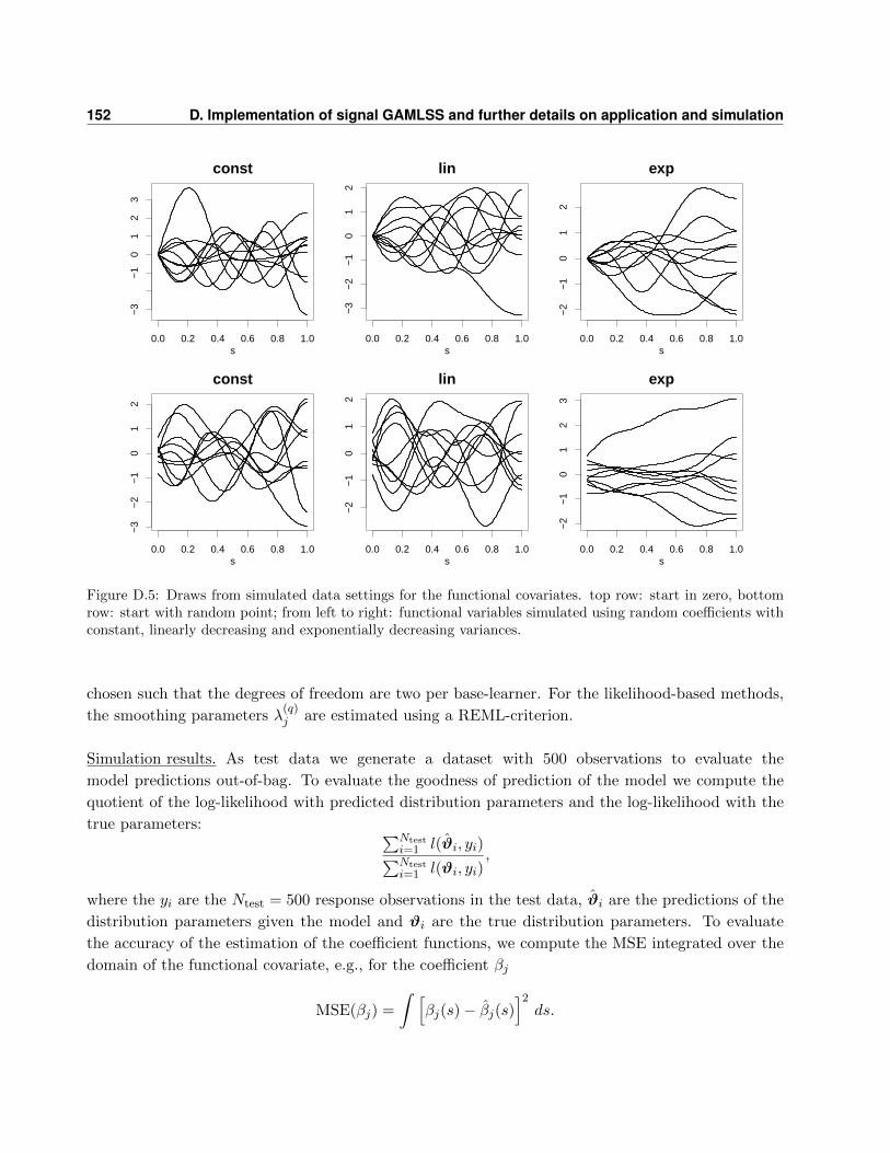
152 D. Implementation of signal GAMLSS and further details on application and simulation
0.0 0.2 0.4 0.6 0.8 1.0
−3
−1
01
23
const
s0.0 0.2 0.4 0.6 0.8 1.0
−3
−2
−1
01
2
lin
s0.0 0.2 0.4 0.6 0.8 1.0
−2
−1
01
2
exp
s
0.0 0.2 0.4 0.6 0.8 1.0
−3
−2
−1
01
2
const
s0.0 0.2 0.4 0.6 0.8 1.0
−2
−1
01
2
lin
s0.0 0.2 0.4 0.6 0.8 1.0
−2
−1
01
23
exp
s
Figure D.5: Draws from simulated data settings for the functional covariates. top row: start in zero, bottomrow: start with random point; from left to right: functional variables simulated using random coefficients withconstant, linearly decreasing and exponentially decreasing variances.
chosen such that the degrees of freedom are two per base-learner. For the likelihood-based methods,
the smoothing parameters λ(q)j are estimated using a REML-criterion.
Simulation results. As test data we generate a dataset with 500 observations to evaluate the
model predictions out-of-bag. To evaluate the goodness of prediction of the model we compute the
quotient of the log-likelihood with predicted distribution parameters and the log-likelihood with the
true parameters: ∑Ntesti=1 l(ϑi, yi)∑Ntesti=1 l(ϑi, yi)
,
where the yi are the Ntest = 500 response observations in the test data, ϑi are the predictions of the
distribution parameters given the model and ϑi are the true distribution parameters. To evaluate
the accuracy of the estimation of the coefficient functions, we compute the MSE integrated over the
domain of the functional covariate, e.g., for the coefficient βj
MSE(βj) =
∫ [βj(s)− βj(s)
]2ds.

D.3 Details of the general simulation study 153
In Figure D.6 the quotient of the log-likelihoods with the predicted and the true parameters is
depicted for the different fitting algorithms, grouped by the complexity of the linear predictors–
constant, linearly or exponentially decreasing variances on the x-axis and the addition of a random
starting value in the bottom row. For the considered settings, all algorithms yield similar values.
coef0 coef1 coef2 coef3
●
●
●
●
●
●●●
● ●●●
● ●● ●●
●
●
●●●
●●● ●●●
●
●●
●●
●
●
●●
●
●
●●
●●
●
●
●●
●
●●
●
●●
●
●
●
● ●
●●●
●
●
●●●●
●
●
● ●
●●●
● ●
●
●
●
●
●
●
●
●
●
●
●
●
●
●
●
●
●
●
●
●
●
●
● ●
●
●
●
●
●
●
●
●●
● ●
●
●
● ●
●●
●
●●●
●
●
●●●
●
●
●
●
●
●
●
●
●
●
●
●
●
●
●
●
●
1.01.01
1.01.01
0rand
const lin exp const lin exp const lin exp const lin exp
l(ϑ)
l(ϑ)
boost gamlss mgcv
Figure D.6: Simulation results for signal GAMLSS. The quotient of the negative log-likelihoods for the predictedand the true distribution parameters in the different data settings with constant, linearly and exponentiallydecreasing variances for the random coefficients generating the functional covariates on the x-axis and functionsstarting in zero or in a random point in rows. The different functional coefficients are given in columns fromcoef0 to coef3. The three fitting algorithms are color-coded. The one-line is marked as in this case the likelihoodof the predicted and the true parameters is equal. Note that all values are displayed on a logarithmic scale.
In the case of zero-coefficients, boosting seems to outperform the other two methods. The quotient
generally becomes higher for more complex linear predictors.
In Figure D.7 the MSE of the coefficient functions α1(s) and β1(s) for the expectation and the
standard deviation, are plotted grouped by the true coefficient function, data generating process
and fitting algorithm. The horizontal 0.1-line is marked, as an MSE smaller 0.1 usually means that
the estimated coefficient function is quite similar to the true one. It can be seen that for equal
settings the functional coefficients in the linear predictor of the expectation are fitted with smaller
MSE than those of the standard deviation. Boosting fits better in the case of zero-coefficients, as
it conducts model selection during estimation. For the other settings, the three estimation methods
yield similar results. Generally, the MSE is smaller for less complex coefficient functions. Comparing
the different data generating processes, the MSE is lowest for constant variances and highest for
exponentially decreasing variances, with the linearly decreasing setting in between, as those settings
generate functional variables with decreasing information contained in the functional covariates. The
only exception is the setting with zero-functional coefficients where all data settings have similar MSE.
There is no big difference between the settings with random starting point and zero as starting point,
which means that the estimation is generally not worse for functional covariates that all start in zero.

154 D. Implementation of signal GAMLSS and further details on application and simulation
The highest MSEs are obtained for the functional coefficient coef3 which is high in the beginning and
then very steep (Figure D.7, far right).
The estimated coefficient functions together with the true coefficient functions are plotted in
Figure D.8 for two data settings: functional covariates with exponentially decreasing variances and
starting point zero (top row) and functional covariates with constant variances and random starting
point. The coefficient functions in the linear predictor of the expectation are estimated more ade-
quately than those of the standard deviation. The estimates are closer to the truth for the more
informative data setting, i.e. they are better for constant than for exponentially decreasing variances.
For the difficult settings, that is decreasing variance in the generation of the functional covariates,
and coef2 or coef3, it can be seen that the coefficient function is sometimes estimated as a constant
line close to or exactly zero.
The functional covariates in the application on stock returns are best reflected by the setting with
exponentially decreasing variances and starting point zero, which is the most difficult data setting.
In this case the absolute value of the coefficients is often underestimated. For settings with more
informative functional covariates, the estimates are mostly close to the true coefficient functions and
the three estimation approaches yield very similar estimates and predictions.
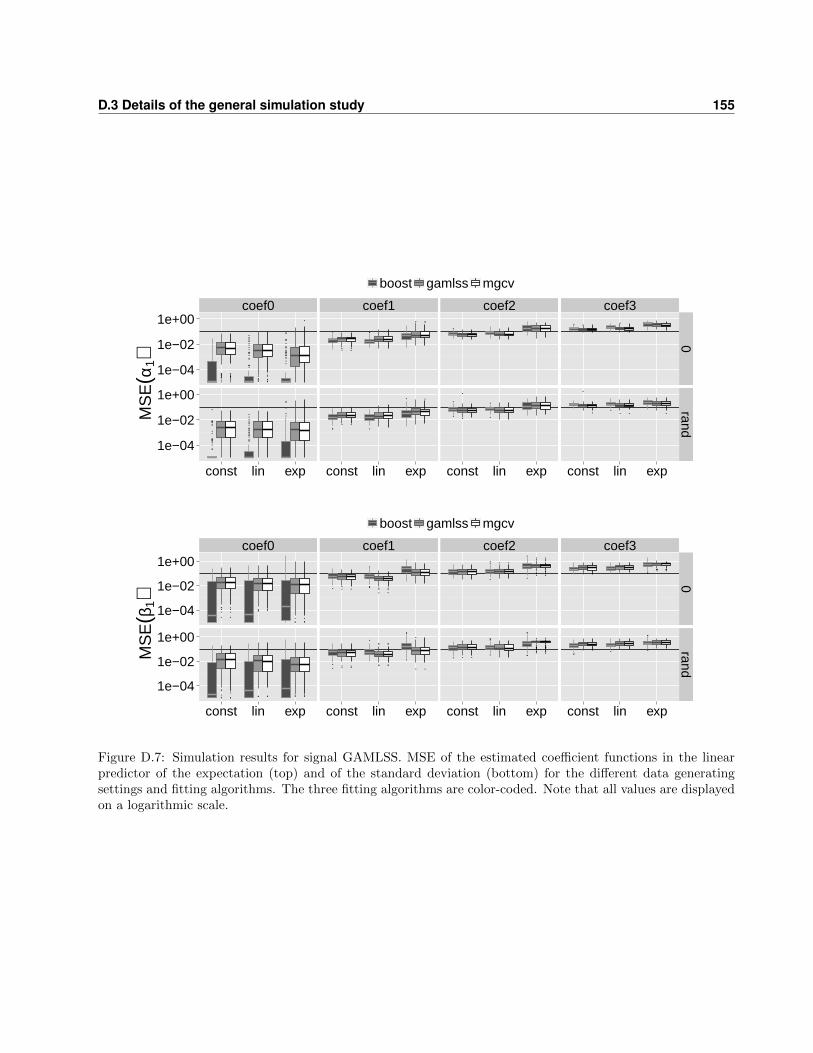
D.3 Details of the general simulation study 155
coef0 coef1 coef2 coef3
●
●
●
●
●●
●●
●●●
● ●
●
●
●
●
●
●
●●
●●
●
●
●
●
●
●
●
●
●
●
●
●
●
●
●
●
●
●
●
●
●
●●
●
●
●●●
●●
●●
●
●
●
●
●
●
●
●
●
●
●●
●
●
●
●
●
●
●
●
●
●
●
●●
●
●
●●●
●
●
●
●
●
●
●
●
●
●
●
●●
●
●●
●
●
●
●
●
●●
●
●
●
●
●
●●
●
●
●
●
●
●
●
●
●
●
●
●
●
●
●●
● ●●
●●
● ●
●
● ●
●
●
●
●
●
●
●
●●
●
●
●
●
● ● ●
1e−04
1e−02
1e+00
1e−04
1e−02
1e+00
0rand
const lin exp const lin exp const lin exp const lin exp
MS
E(α
1)
boost gamlss mgcv
coef0 coef1 coef2 coef3
●
●
●●
●
●
●
●
●
●
●●
●●
●
●●
●
●●
●
●●
●
●●
●●
●
●
●● ●● ●●
●
●●
●
●
●
● ●
●●●
●
●
●●
●
●●
●
●
●
●
●●
●
●
●
●
●
●
●
●
●
●
●●
●
● ●
●
●
● ● ●
●
●
●
●
●●
●
●●
●
●
●●
●
●
●●
●
●
● ● ●
●
●
●●
●
●●
●
●
●●
●
●
●
●
●●●●
●
●
●
●●
●
●
●
●●
●
●
●
●
●
●
●●●●
●
●
●
●●
●
●
●●
●●●●
●●●●●
●
●●
●
●●
●
●
●
1e−04
1e−02
1e+00
1e−04
1e−02
1e+00
0rand
const lin exp const lin exp const lin exp const lin exp
MS
E(β
1)
boost gamlss mgcv
Figure D.7: Simulation results for signal GAMLSS. MSE of the estimated coefficient functions in the linearpredictor of the expectation (top) and of the standard deviation (bottom) for the different data generatingsettings and fitting algorithms. The three fitting algorithms are color-coded. Note that all values are displayedon a logarithmic scale.
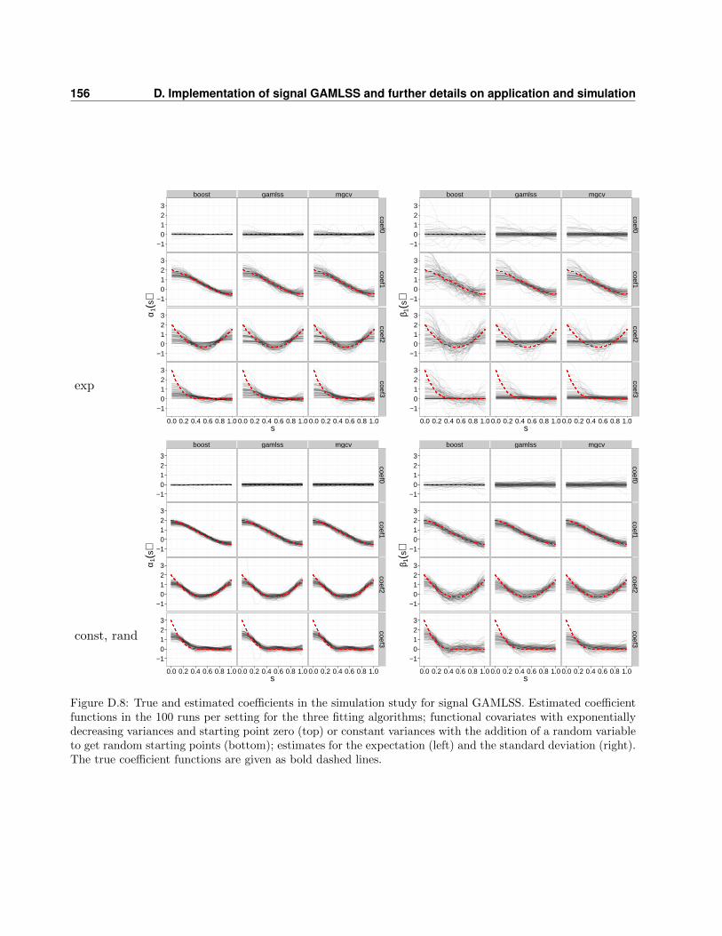
156 D. Implementation of signal GAMLSS and further details on application and simulation
exp
boost gamlss mgcv
−10123
−10123
−10123
−10123
coef0coef1
coef2coef3
0.0 0.2 0.4 0.6 0.8 1.0 0.0 0.2 0.4 0.6 0.8 1.0 0.0 0.2 0.4 0.6 0.8 1.0s
α 1(s
)
boost gamlss mgcv
−10123
−10123
−10123
−10123
coef0coef1
coef2coef3
0.0 0.2 0.4 0.6 0.8 1.0 0.0 0.2 0.4 0.6 0.8 1.0 0.0 0.2 0.4 0.6 0.8 1.0s
β 1(s
)
const, rand
boost gamlss mgcv
−10123
−10123
−10123
−10123
coef0coef1
coef2coef3
0.0 0.2 0.4 0.6 0.8 1.0 0.0 0.2 0.4 0.6 0.8 1.0 0.0 0.2 0.4 0.6 0.8 1.0s
α 1(s
)
boost gamlss mgcv
−10123
−10123
−10123
−10123
coef0coef1
coef2coef3
0.0 0.2 0.4 0.6 0.8 1.0 0.0 0.2 0.4 0.6 0.8 1.0 0.0 0.2 0.4 0.6 0.8 1.0s
β 1(s
)
Figure D.8: True and estimated coefficients in the simulation study for signal GAMLSS. Estimated coefficientfunctions in the 100 runs per setting for the three fitting algorithms; functional covariates with exponentiallydecreasing variances and starting point zero (top) or constant variances with the addition of a random variableto get random starting points (bottom); estimates for the expectation (left) and the standard deviation (right).The true coefficient functions are given as bold dashed lines.
Appendix E
Further details on the R package
FDboost
E.1 Base-learners for functional covariates
The base-learner bsignal() sets up a linear effect of a functional variable∫S xj(s)βj(s) ds. We ap-
proximate the integral numerically as a weighted sum using integration weights ∆(s) (Wood, 2011).
Define xj(sr) = ∆(sr)xj(sr), r = 1, . . . , R, the basis for the covariate is computed as
bj(x)> ≈ [xj(s1) · · · xj(sR)] [Φj(s1) · · · Φj(sR)]>
=
[R∑r=1
xj(sr)Φ1(sr) · · ·R∑r=1
xj(sr)ΦKj (sr)
],
where Φj(sr) is a vector of Kj B-splines evaluated at sr. The corresponding penalty matrix P j is a
squared difference matrix. Thus, the smooth effect in s is represented by P-splines (Eilers and Marx,
1996).
Using the base-learner bfpc() the linear functional effect∫S xj(s)βj(s) ds is specified using a FPC
basis. The functional covariate xj(s) and the coefficient βj(s) are both represented in the basis that
is spanned by the functional principal components (FPCs, see, e.g., Ramsay and Silverman, 2005,
Chap. 8 and 9) of xj(s). Let Xj(s) be a zero-mean stochastic process in the L2(S) (i.e., square-
integrable). We have observations xij(s) from this process. We denote the eigenvalues of the auto-
covariance of Xj(s) as ζ1 ≥ ζ2 ≥ · · · ≥ 0 and the corresponding eigenfunctions as ek(s), k ∈ N. The
eigenfunctions {ek(s), k ∈ N} form an orthonormal basis for the L2(S). Using the Karhunen-Loeve
theorem, the functional covariate can be represented as weighted sum
Xij(s) =∞∑k=1
Zikek(s),
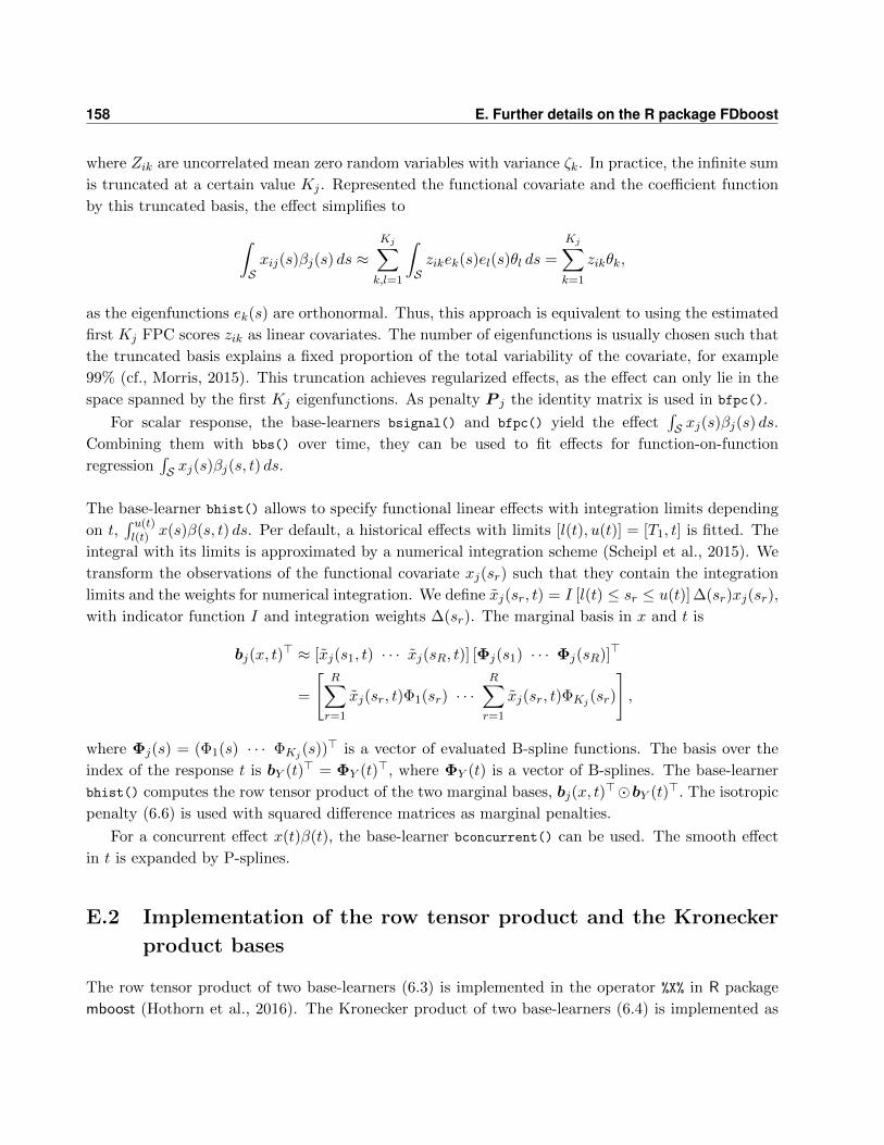
158 E. Further details on the R package FDboost
where Zik are uncorrelated mean zero random variables with variance ζk. In practice, the infinite sum
is truncated at a certain value Kj . Represented the functional covariate and the coefficient function
by this truncated basis, the effect simplifies to
∫Sxij(s)βj(s) ds ≈
Kj∑k,l=1
∫Szikek(s)el(s)θl ds =
Kj∑k=1
zikθk,
as the eigenfunctions ek(s) are orthonormal. Thus, this approach is equivalent to using the estimated
first Kj FPC scores zik as linear covariates. The number of eigenfunctions is usually chosen such that
the truncated basis explains a fixed proportion of the total variability of the covariate, for example
99% (cf., Morris, 2015). This truncation achieves regularized effects, as the effect can only lie in the
space spanned by the first Kj eigenfunctions. As penalty P j the identity matrix is used in bfpc().
For scalar response, the base-learners bsignal() and bfpc() yield the effect∫S xj(s)βj(s) ds.
Combining them with bbs() over time, they can be used to fit effects for function-on-function
regression∫S xj(s)βj(s, t) ds.
The base-learner bhist() allows to specify functional linear effects with integration limits depending
on t,∫ u(t)l(t) x(s)β(s, t) ds. Per default, a historical effects with limits [l(t), u(t)] = [T1, t] is fitted. The
integral with its limits is approximated by a numerical integration scheme (Scheipl et al., 2015). We
transform the observations of the functional covariate xj(sr) such that they contain the integration
limits and the weights for numerical integration. We define xj(sr, t) = I [l(t) ≤ sr ≤ u(t)] ∆(sr)xj(sr),
with indicator function I and integration weights ∆(sr). The marginal basis in x and t is
bj(x, t)> ≈ [xj(s1, t) · · · xj(sR, t)] [Φj(s1) · · · Φj(sR)]>
=
[R∑r=1
xj(sr, t)Φ1(sr) · · ·R∑r=1
xj(sr, t)ΦKj (sr)
],
where Φj(s) = (Φ1(s) · · · ΦKj (s))> is a vector of evaluated B-spline functions. The basis over the
index of the response t is bY (t)> = ΦY (t)>, where ΦY (t) is a vector of B-splines. The base-learner
bhist() computes the row tensor product of the two marginal bases, bj(x, t)>�bY (t)>. The isotropic
penalty (6.6) is used with squared difference matrices as marginal penalties.
For a concurrent effect x(t)β(t), the base-learner bconcurrent() can be used. The smooth effect
in t is expanded by P-splines.
E.2 Implementation of the row tensor product and the Kronecker
product bases
The row tensor product of two base-learners (6.3) is implemented in the operator %X% in R package
mboost (Hothorn et al., 2016). The Kronecker product of two base-learners (6.4) is implemented as
E.2 Implementation of the row tensor product and the Kronecker product bases 159
%O%. When %X% or %O% is called with a specification of df in both marginal base-learners, the df of
the composed effect are computed as the product of the two specified df. Then, only one smoothing
parameter is computed for an isotropic penalty like in (6.6).
Consider, for example, the composed base-learner bols(z1, df = df1) %O% bbs(t, df = df2).
The base-learner bols() specifies a linear effect. The base-learner bbs() specifies a smooth effect
represented by P-splines (Eilers and Marx, 1996). Thus, the composed base-learner yields the effect
z1βj(t), which is linear in z1 and smooth in t. The global df for the composed base-learner are
computed as dfj = df1 * df2. The corresponding smoothing parameter λj is computed by Demmler-
Reinsch orthogonalization (Ruppert et al., 2003, Appendix B.1.1).
The anisotropic penalty (6.5) is obtained if the smoothing parameter is specified in both marginal
base-learners; for instance, as bols(z1, lambda = lambda1) %O% bbs(t, lambda = lambda2). However,
it is hard to control the df in this case such that each base-learner in the model has the same number
of dfs.
In some cases, one only wants to penalize the basis in t direction. For that, the penalty in (6.7) can
be used. Such a penalty is obtained using %A0% or %Xa0%, for the Kronecker and the row tensor product
basis, respectively. When %A0% or %Xa0% are used to form an effect with penalty (6.7), the number of
df in the first base-learner has to be equal to the number of its columns. Consider, bols(z1, df =
1, intercept = FALSE) %A0% bbs(t, df = df2), with a metric variable z1. This specification implies
bj(xi) = xi1 and P j = 0 for the bols() base-learner. The bbs() base-learner sets up a design matrix
of B-spline evaluations in t and a squared difference matrix as penalty matrix.
Linking formula and timeformula in FDboost() to representation (6.3) and (6.4), the J base-
learners in formula correspond to the J marginal bases bj and the base-learners in timeformula
corresponds to the marginal basis bY . If it is possible to represent the effects as Kronecker product,
the base-learners are combined by %O%. Otherwise, the row tensor product %X% is used to combine the
marginal bases.
Consider, for example, formula = Y ∼ b1(x) + b2(x) + ... + bJ(x), and the timeformula =
∼ bY (t). For an array model, this yields formula = Y ∼ b1(x) %O% bY (t) + b2(x) %O% bY (t) +
... + bJ(x) %O% bY (t). In model (6.1), this corresponds to the linear predictor hj(x)(t) =∑j (bj(x)⊗ bY (t))θj . If formula contains base-learners that are composed of two base-learners by
%O% or %A0%, those effects are not expanded with timeformula, allowing for model specifications with
different effects in t direction.

160 E. Further details on the R package FDboost

References
Amihud, Y. (2002). Illiquidity and stock returns: cross-section and time-series effects. Journal of
Financial Markets, 5(1):31–56.
Amihud, Y., Mendelson, H., and Pedersen, L. H. (2013). Market Liquidity: Asset Pricing, Risk, and
Crises. Cambridge University Press, Cambridge.
Antoch, J., Prchal, L., Rosaria De Rosa, M., and Sarda, P. (2010). Electricity consumption prediction
with functional linear regression using spline estimators. Journal of Applied Statistics, 37(12):2027–
2041.
Baladandayuthapani, V., Mallick, B. K., Young Hong, M., Lupton, J. R., Turner, N. D., and Carroll,
R. J. (2008). Bayesian hierarchical spatially correlated functional data analysis with application to
colon carcinogenesis. Biometrics, 64(1):64–73.
Bauer, E. and Kohavi, R. (1999). An empirical comparison of voting classification algorithms: bag-
ging, boosting, and variants. Machine Learning, 36(1-2):105–139.
Binder, H. and Schumacher, M. (2008). Allowing for mandatory covariates in boosting estimation of
sparse high-dimensional survival models. BMC Bioinformatics, 9(1):1–10.
Bollerslev, T. (1986). Generalized autoregressive conditional heteroskedasticity. Journal of Econo-
metrics, 31(3):307–327.
Breiman, L. (1998). Arcing classifiers (with discussion and a rejoinder by the author). The Annals
of Statistics, 26(3):801–849.
Breiman, L. (1999). Prediction games and arcing algorithms. Neural Computation, 11(7):1493–1517.
Brewer, J. (1978). Kronecker products and matrix calculus in system theory. IEEE Transactions on
circuits and systems, 25(9):772–781.
Brockhaus, S., Fuest, A., Mayr, A., and Greven, S. (2015a). Functional regression models for location,
scale and shape applied to stock returns. In Herwig, F. and Helga, W., editors, Proceedings of the
30th International Workshop on Statistical Modelling, pages 117–122.

162 REFERENCES
Brockhaus, S., Fuest, A., Mayr, A., and Greven, S. (2016a). Signal regression models for location,
scale and shape with an application to stock returns. arXiv preprint, arXiv:1605.04281.
Brockhaus, S., Melcher, M., Leisch, F., and Greven, S. (2016b). Boosting flexible functional regression
models with a high number of functional historical effects. Statistics and Computing. Accepted,
DOI: http://dx.doi.org/10.1007/s11222-016-9662-1.
Brockhaus, S. and Rugamer, D. (2016). FDboost: Boosting Functional Regression Models. R package
version 0.2-0, Available at http://CRAN.R-project.org/package=FDboost/.
Brockhaus, S., Scheipl, F., Hothorn, T., and Greven, S. (2014). The functional linear array model
and an application to viscosity curves. In Kneib, T., Sobotka, F., Fahrenholz, J., and Irmer, H.,
editors, Proceedings of the 29th International Workshop on Statistical Modelling, pages 63–68.
Brockhaus, S., Scheipl, F., Hothorn, T., and Greven, S. (2015b). The functional linear array model.
Statistical Modelling, 15(3):279–300.
Buhlmann, P. and Hothorn, T. (2007). Boosting algorithms: regularization, prediction and model
fitting (with discussion). Statistical Science, 22(4):477–505.
Buhlmann, P. and Yu, B. (2003). Boosting with the L2 loss: regression and classification. Journal of
the American Statistical Association, 98(462):324–339.
Buja, A., Hastie, T. J., and Tibshirani, R. J. (1989). Linear smoothers and additive models. The
Annals of Statistics, 17(2):453–510.
Cardot, H., Crambes, C., and Sarda, P. (2005). Quantile regression when the covariates are functions.
Nonparametric Statistics, 17(7):841–856.
Carlstein, E. (1986). The use of subseries values for estimating the variance of a general statistic from
a stationary sequence. The Annals of Statistics, 14(3):1171–1179.
Cederbaum, J., Pouplier, M., Hoole, P., and Greven, S. (2016). Functional linear mixed models for
irregularly or sparsely sampled data. Statistical Modelling, 16(1):67–88.
Chen, K. and Muller, H.-G. (2012a). Conditional quantile analysis when covariates are functions,
with application to growth data. Journal of the Royal Statistical Society: Series B (Statistical
Methodology), 74(1):67–89.
Chen, K. and Muller, H.-G. (2012b). Modeling repeated functional observations. Journal of the
American Statistical Association, 107(500):1599–1609.
Cole, T. J. and Green, P. J. (1992). Smoothing reference centile curves: the LMS method and
penalized likelihood. Statistics in Medicine, 11(10):1305–1319.
REFERENCES 163
Cont, R. (2001). Empirical properties of asset returns: stylized facts and statistical issues. Quantita-
tive Finance, 1(2):223–236.
Crainiceanu, C. M., Caffo, B. S., Luo, S., Zipunnikov, V. M., and Punjabi, N. M. (2012). Population
value decomposition, a framework for the analysis of image populations. Journal of the American
Statistical Association, 106(495):775–790.
Crainiceanu, C. M., Staicu, A.-M., and Di, C.-Z. (2009). Generalized multilevel functional regression.
Journal of the American Statistical Association, 104(488):1550–1561.
Cuevas, A. (2014). A partial overview of the theory of statistics with functional data. Journal of
Statistical Planning and Inference, 147(0):1–23.
Currie, I. D., Durban, M., and Eilers, P. H. C. (2006). Generalized linear array models with applica-
tions to multidimensional smoothing. Journal of the Royal Statistical Society: Series B (Statistical
Methodology), 68(2):259–280.
Di, C.-Z., Crainiceanu, C. M., Caffo, B. S., and Punjabi, N. M. (2009). Multilevel functional principal
component analysis. The Annals of Applied Statistics, 3(1):458–488.
Dunn, P. K. and Smyth, G. K. (1996). Randomized quantile residuals. Journal of Computational
and Graphical Statistics, 5(3):236–244.
Eilers, P. H. C. and Marx, B. D. (1996). Flexible smoothing with B-splines and penalties (with
comments and rejoinder). Statistical Science, 11(2):89–121.
Engle, R. F. (1982). Autoregressive conditional heteroscedasticity with estimates of the variance of
United Kingdom inflation. Econometrica: Journal of the Econometric Society, 50(4):987–1008.
Febrero-Bande, M., Galeano, P., and Gonzalez-Manteiga, W. (2015). Functional principal component
regression and functional partial least-squares regression: an overview and a comparative study.
International Statistical Review. Accepted, DOI: http://dx.doi.org/10.1111/insr.12116,.
Fenske, N., Kneib, T., and Hothorn, T. (2011). Identifying risk factors for severe childhood malnu-
trition by boosting additive quantile regression. Journal of the American Statistical Association,
106(494):494–510.
Ferraty, F., editor (2011). Recent Advances in Functional Data Analysis and Related Topics. Springer,
Berlin Heidelberg.
Ferraty, F., Mas, A., and Vieu, P. (2007). Nonparametric regression on functional data: Inference
and practical aspects. Australian & New Zealand Journal of Statistics, 49(3):267–286.
Ferraty, F., Rabhi, A., and Vieu, P. (2005). Conditional quantiles for dependent functional data
with application to the climatic El Nino phenomenon. Sankhya: The Indian Journal of Statistics,
67(2):378–398.
164 REFERENCES
Ferraty, F. and Romain, Y., editors (2011). The Oxford Handbook of Functional Data Analysis.
Oxford University Press, Oxford.
Ferraty, F., Van Keilegom, I., and Vieu, P. (2012). Regression when both response and predictor are
functions. Journal of Multivariate Analysis, 109:10–28.
Ferraty, F. and Vieu, P. (2006). Nonparametric Functional Data Analysis. Springer Series in Statistics.
Springer, New York. Theory and practice.
Ferraty, F. and Vieu, P. (2009). Additive prediction and boosting for functional data. Computational
Statistics & Data Analysis, 53(4):1400–1413.
Freund, Y. and Schapire, R. E. (1996). Experiments with a new boosting algorithm. In Proceedings of
the Thirteenth International Conference on Machine Learning, volume 96, pages 148–156. Morgan
Kaufmann Publishers Inc., San Francisco, CA.
Freund, Y. and Schapire, R. E. (1997). A decision-theoretic generalization of on-line learning and an
application to boosting. Journal of Computer and System Sciences, 55(1):119–139.
Fried, R., Schettlinger, K., and Borowski, M. (2012). robfilter: Robust Time Series Filters. R package
version 4.0, Available at http://CRAN.R-project.org/package=robfilter.
Friedman, J. H. (2001). Greedy function approximation: a gradient boosting machine. The Annals
of Statistics, 29(5):1189–1232.
Friedman, J. H., Hastie, T., and Tibshirani, R. (2000). Additive logistic regression: a statistical view
of boosting (with discussion and a rejoinder by the authors). The Annals of Statistics, 28(2):337–
407.
Fuchs, K., Scheipl, F., and Greven, S. (2015). Penalized scalar-on-functions regression with interaction
term. Computational Statistics & Data Analysis, 81:38–51.
Fuest, A. and Mittnik, S. (2015). Modeling liquidity impact on volatility: a GARCH-FunXL approach.
Technical Report 15, Center for Quantitative Risk Analysis (CEQURA).
Gellar, J. E., Colantuoni, E., Needham, D. M., and Crainiceanu, C. M. (2014). Variable-domain
functional regression for modeling ICU data. Journal of the American Statistical Association,
109(508):1425–1439.
Gertheiss, J., Maity, A., and Staicu, A.-M. (2013). Variable selection in generalized functional linear
models. Stat, 2(1):86–101.
Gervini, D. (2015). Dynamic retrospective regression for functional data. Technometrics, 57(1):26–34.
Goia, A. and Vieu, P. (2016). An introduction to recent advances in high/infinite dimensional statis-
tics. Journal of Multivariate Analysis, 146(4):1–6.

REFERENCES 165
Goldsmith, J., Bobb, J., Crainiceanu, C. M., Caffo, B. S., and Reich, D. S. (2011). Penalized functional
regression. Journal of Computational and Graphical Statistics, 20(4):830–851.
Goldsmith, J., Greven, S., and Crainiceanu, C. M. (2013). Corrected confidence bands for functional
data using principal components. Biometrics, 69(1):41–51.
Goldsmith, J., Huang, L., and Crainiceanu, C. M. (2014). Smooth scalar-on-image regression via
spatial Bayesian variable selection. Journal of Computational and Graphical Statistics, 23(1):46–
64.
Greven, S. (2015). A general framework for functional regression. In Herwig, F. and Helga, W.,
editors, Proceedings of the 30th International Workshop on Statistical Modelling, pages 39–54.
Greven, S., Crainiceanu, C. M., Caffo, B. S., and Reich, D. S. (2010). Longitudinal functional principal
component analysis. Electronic Journal of Statistics, 4:1022–1054.
Hardle, W. K., Hautsch, N., and Mihoci, A. (2012). Modelling and forecasting liquidity supply using
semiparametric factor dynamics. Journal of Empirical Finance, 19(4):610–625.
Harezlak, J., Coull, B. A., Laird, N. M., Magari, S. R., and Christiani, D. C. (2007). Penalized
solutions to functional regression problems. Computational Statistics & Data Analysis, 51(10):4911–
4925.
Hastie, T. J. and Tibshirani, R. J. (1986). Generalized additive models. Statistical Science, 1(3):297–
310.
Hastie, T. J. and Tibshirani, R. J. (1993). Varying-coefficient models. Journal of the Royal Statistical
Society: Series B (Statistical Methodology), 55(4):757–796.
Herrick, R. (2015). WFMM. The University of Texas M.D. Anderson Cancer Center, version 3.0
edition.
Hofner, B., Boccuto, L., and Goker, M. (2015a). Controlling false discoveries in high-dimensional
situations: Boosting with stability selection. BMC Bioinformatics, 16(1):1–17.
Hofner, B., Hothorn, T., Kneib, T., and Schmid, M. (2011). A framework for unbiased model selection
based on boosting. Journal of Computational and Graphical Statistics, 20(4):956–971.
Hofner, B., Kneib, T., and Hothorn, T. (2016). A unified framework of constrained regression.
Statistics and Computing, 26(1):1–14.
Hofner, B., Mayr, A., Fenske, N., and Schmid, M. (2015b). gamboostLSS: Boosting Methods for
GAMLSS Models. R package version 1.2-0, Available at http://CRAN.R-project.org/package=
gamboostLSS.
166 REFERENCES
Hofner, B., Mayr, A., Robinzonov, N., and Schmid, M. (2014). Model-based boosting in R: a hands-on
tutorial using the R package mboost. Computational Statistics, 29(1):3–35.
Hofner, B., Mayr, A., and Schmid, M. (2015c). gamboostlss: An R package for model building and
variable selection in the GAMLSS framework. Journal of Statistical Software. Accepted, arXiv
preprint, arXiv:1407.1774.
Horvath, L. and Kokoszka, P. (2012). Inference for Functional Data with Applications, volume 200
of Springer Series in Statistics. Springer Science & Business Media New York.
Hothorn, T. (2013). ctm: Conditional Transformation Models. R package version 0.0-3, Available at
https://r-forge.r-project.org/projects/ctm/.
Hothorn, T., Buhlmann, P., Dudoit, S., Molinaro, A., and Van Der Laan, M. J. (2006). Survival
ensembles. Biostatistics, 7(3):355–373.
Hothorn, T., Buhlmann, P., Kneib, T., Schmid, M., and Hofner, B. (2016). mboost: Model-Based
Boosting. R package version 2.6-0, Available at http://CRAN.R-project.org/package=mboost.
Hothorn, T., Kneib, T., and Buhlmann, P. (2013). Conditional transformation models. Journal of
the Royal Statistical Society: Series B (Statistical Methodology), 76(1):3–27.
Hsing, T. and Eubank, R. (2015). Theoretical Foundations of Functional Data Analysis, with an
Introduction to Linear Operators. John Wiley & Sons.
Huang, L., Scheipl, F., Goldsmith, J., Gellar, J. E., Harezlak, J., McLean, M. W., Swihart, B., Xiao,
L., Crainiceanu, C. M., and Reiss, P. T. (2016). refund: Regression with Functional Data. R package
version 0.1-14, Available at https://cran.r-project.org/package=refund.
Huber, P. J. (1964). Robust estimation of a location parameter. The Annals of Mathematical Statistics,
35(1):73–101.
Ivanescu, A. E., Staicu, A.-M., Scheipl, F., and Greven, S. (2015). Penalized function-on-function
regression. Computational Statistics, 30(2):539–568.
Jacques, J. and Preda, C. (2014). Functional data clustering: A survey. Advances in Data Analysis
and Classification, 8(3):231–255.
James, G. M. and Silverman, B. W. (2005). Functional adaptive model estimation. Journal of the
American Statistical Association, 100(470):565–576.
James, G. M., Wang, J., and Zhu, J. (2009). Functional linear regression that’s interpretable. The
Annals of Statistics, 37(5A):2083–2108.
Kim, J. S., Maity, A., and Staicu, A.-M. (2016). Generalized functional concurrent model. Unpub-
lished manuscript.
REFERENCES 167
Kim, K., Senturk, D., and Li, R. (2011). Recent history functional linear models for sparse longitudinal
data. Journal of Statistical Planning and Inference, 141(4):1554–1566.
Klein, N., Kneib, T., Lang, S., and Sohn, A. (2015). Bayesian structured additive distributional
regression with an application to regional income inequality in Germany. The Annals of Applied
Statistics, 9(2):1024–1052.
Kneib, T. (2013). Beyond mean regression. Statistical Modelling, 13(4):275–303.
Kneib, T., Hothorn, T., and Tutz, G. (2009). Variable selection and model choice in geoadditive
regression models. Biometrics, 65(2):626–634.
Koenker, R. (2005). Quantile Regression. Cambridge University Press, Cambridge.
Koenker, R. and Bassett, G. (1978). Regression quantiles. Econometrica: Journal of the Econometric
Society, pages 33–50.
Kokoszka, P. (2012). Dependent functional data. ISRN Probability and Statistics, 2012:1–30. Article
ID 958254.
Kramer, N. (2006). Boosting for functional data. In Rizzi, A. and Vichi, M., editors, COMPSTAT
2006—Proceedings in Computational Statistics, pages 1121–1128. Physica Verlag, Heidelberg, Ger-
many.
Lange, K. L., Little, R. J. A., and Taylor, J. M. G. (1989). Robust statistical modeling using the
t distribution. Journal of the American Statistical Association, 84(408):881–896.
Larsson, R. and Villani, M. (2001). A distance measure between cointegration spaces. Economics
Letters, 70(1):21–27.
Lopez-Pintado, S. and Romo, J. (2009). On the concept of depth for functional data. Journal of the
American Statistical Association, 104(486):718–734.
Luchner, M., Gutmann, R., Bayer, K., Dunkl, J., Hansel, A., Herbig, J., Singer, W., Strobl, F., Win-
kler, K., and Striedner, G. (2012). Implementation of proton transfer reaction-mass spectrometry
(PTR-MS) for advanced bioprocess monitoring. Biotechnology and Bioengineering, 109(12):3059–
3069.
Malfait, N. and Ramsay, J. O. (2003). The historical functional linear model. Canadian Journal of
Statistics, 31(2):115–128.
Malloy, E. J., Morris, J. S., Adar, S. D., Suh, H., Gold, D. R., and Coull, B. A. (2010). Wavelet-
based functional linear mixed models: an application to measurement error–corrected distributed
lag models. Biostatistics, 11(3):432–452.

168 REFERENCES
Marra, G. and Wood, S. N. (2011). Practical variable selection for generalized additive models.
Computational Statistics & Data Analysis, 55(7):2372–2387.
Marron, J. S., Ramsay, J. O., Sangalli, L. M., and Srivastava, A. (2014). Statistics of time warpings
and phase variations. Electronic Journal of Statistics, 8(2):1697–1702.
Marx, B. D. and Eilers, P. H. C. (1999). Generalized linear regression on sampled signals and curves:
a P-spline approach. Technometrics, 41(1):1–13.
Mayr, A., Binder, H., Gefeller, O., and Schmid, M. (2014a). The evolution of boosting algorithms.
Methods of Information in Medicine, 53(6):419–427.
Mayr, A., Binder, H., Gefeller, O., and Schmid, M. (2014b). Extending statistical boosting. Methods
of Information in Medicine, 53(6):428–435.
Mayr, A., Fenske, N., Hofner, B., Kneib, T., and Schmid, M. (2012). Generalized additive models
for location, scale and shape for high dimensional data – a flexible approach based on boosting.
Journal of the Royal Statistical Society: Series C (Applied Statistics), 61(3):403–427.
Mayr, A., Schmid, M., Pfahlberg, A., Uter, W., and Gefeller, O. (2015). A permutation test to
analyse systematic bias and random measurement errors of medical devices via boosting location
and scale models. Statistical Methods in Medical Research. Accepted.
McLean, M. W., Hooker, G., Staicu, A.-M., Scheipl, F., and Ruppert, D. (2014). Functional gener-
alized additive models. Journal of Computational and Graphical Statistics, 23(1):249–269.
Meinshausen, N. and Buhlmann, P. (2010). Stability selection (with discussion). Journal of the Royal
Statistical Society: Series B (Statistical Methodology), 72(4):417–473.
Melcher, M., Scharl, T., Spangl, B., Luchner, M., Cserjan, M., Bayer, K., Leisch, F., and Striedner, G.
(2015). The potential of random forest and neural networks for biomass and recombinant protein
modeling in Escherichia coli fed-batch fermentations. Biotechnology Journal, 10(11):1770–1782.
Meyer, M. J., Coull, B. A., Versace, F., Cinciripini, P., and Morris, J. S. (2015). Bayesian function-
on-function regression for multilevel functional data. Biometrics, 71(3):563–574.
Morris, J. S. (2015). Functional regression. Annual Review of Statistics and Its Application, 2(1):321–
359.
Morris, J. S., Arroyo, C., Coull, B. A., Ryan, L. M., Herrick, R., and Gortmaker, S. L. (2006). Using
wavelet-based functional mixed models to characterize population heterogeneity in accelerometer
profiles: a case study. Journal of the American Statistical Association, 101(476):1352–1364.
Morris, J. S. and Carroll, R. J. (2006). Wavelet-based functional mixed models. Journal of the Royal
Statistical Society: Series B (Statistical Methodology), 68(2):179–199.

REFERENCES 169
Most, L. and Hothorn, T. (2015). Conditional transformation models for survivor function estimation.
The International Journal of Biostatistics, 11(1):23–50.
Muller, H.-G. and Stadtmuller, U. (2005). Generalized functional linear models. The Annals of
Statistics, 33(2):774–805.
Muller, H.-G., Wu, Y., and Yao, F. (2013). Continuously additive models for nonlinear functional
regression. Biometrika, 100(3):607–622.
Muller, H.-G. and Yao, F. (2008). Functional additive models. Journal of the American Statistical
Association, 103(484):1534–1544.
Nelder, J. A. and Wedderburn, R. W. M. (1972). Generalized linear models. Journal of the Royal
Statistical Society: Series A (Statistics in Society), 135(3):370–384.
Newey, W. K. and Powell, J. L. (1987). Asymmetric least squares estimation and testing. Economet-
rica: Journal of the Econometric Society, 55(4):819–847.
Obermeier, V., Scheipl, F., Heumann, C., Wassermann, J., and Kuchenhoff, H. (2014). Flexible
distributed lags for modelling earthquake data. Journal of the Royal Statistical Society: Series C
(Applied Statistics), 64(2):231–412.
Patterson, H. D. and Thompson, R. (1971). Recovery of inter-block information when block sizes are
unequal. Biometrika, 58(3):545–554.
R Core Team (2015). R: A Language and Environment for Statistical Computing. R Foundation for
Statistical Computing, Vienna, Austria. R 3.2.3, Available at http://www.R-project.org/.
Ramsay, J. O. and Dalzell, C. J. (1991). Some tools for functional data analysis (with discussion).
Journal of the Royal Statistical Society: Series B (Statistical Methodology), 53(3):539–572.
Ramsay, J. O. and Li, X. (1998). Curve registration. Journal of the Royal Statistical Society: Series
B (Statistical Methodology), 60(2):351–363.
Ramsay, J. O. and Silverman, B. W. (2005). Functional Data Analysis. Springer, New York.
Ramsay, J. O., Wickham, H., Graves, S., and Hooker, G. (2014). fda: Functional Data Analysis.
R package version 2.4.4, Available at http://CRAN.R-project.org/package=fda.
Reiss, P. T., Huang, L., and Mennes, M. (2010). Fast function-on-scalar regression with penalized
basis expansions. The International Journal of Biostatistics, 6(1):1–30.
Reiss, P. T. and Ogden, R. T. (2007). Functional principal component regression and functional
partial least squares. Journal of the American Statistical Association, 102(479):984–996.
Ridgeway, G. (1999). The state of boosting. Computing Science and Statistics, 31:172–181.

170 REFERENCES
Ridgeway, G. (2002). Looking for lumps: boosting and bagging for density estimation. Computational
Statistics & Data Analysis, 38(4):379–392.
Rigby, R. A. and Stasinopoulos, D. M. (1996). A semi-parametric additive model for variance het-
erogeneity. Statistics and Computing, 6(1):57–65.
Rigby, R. A. and Stasinopoulos, D. M. (2005). Generalized additive models for location, scale and
shape (with discussion). Journal of the Royal Statistical Society: Series C (Applied Statistics),
54(3):507–554.
Rigby, R. A. and Stasinopoulos, D. M. (2014). Automatic smoothing parameter selection in GAMLSS
with an application to centile estimation. Statistical Methods in Medical Research, 23(4):318–332.
Rigby, R. A. and Stasinopoulos, D. M. (2015). gamlss.add: Extra Additive Terms for GAMLSS Models.
R package version 4.3-4, Available at http://CRAN.R-project.org/package=gamlss.add.
Rosset, S., Zhu, J., and Hastie, T. J. (2004). Boosting as a regularized path to a maximum margin
classifier. The Journal of Machine Learning Research, 5:941–973.
Rugamer, D., Brockhaus, S., Gentsch, K., Scherer, K., and Greven, S. (2016). Detecting synchronisa-
tion in EEG- and EMG-signals via boosted functional historical models. Unpublished manuscript.
Ruppert, D., Wand, M. P., and Carroll, R. J. (2003). Semiparametric Regression. Cambridge Uni-
versity Press.
Schapire, R. E. (2003). The boosting approach to machine learning: an overview. In Denison,
D. D., Hansen, M. H., Holmes, C. C., Mallick, B., and Yu, B., editors, Nonlinear Estimation and
Classification, volume 171, pages 149–171. Springer, New York.
Schapire, R. E. and Freund, Y. (2012). Boosting: Foundations and Algorithms. MIT Press, Cambridge,
London.
Scheipl, F., Gertheiss, J., and Greven, S. (2016). Generalized functional additive mixed models.
Electronic Journal of Statistics, 10(1):1455–1492.
Scheipl, F. and Greven, S. (2016). Identifiability in penalized function-on-function regression models.
Electronic Journal of Statistics, 10(1):495–526.
Scheipl, F., Staicu, A.-M., and Greven, S. (2015). Functional additive mixed models. Journal of
Computational and Graphical Statistics, 24(2):477–501.
Schmid, M. and Hothorn, T. (2008a). Boosting additive models using component-wise P-splines.
Computational Statistics & Data Analysis, 53(2):298–311.
Schmid, M. and Hothorn, T. (2008b). Flexible boosting of accelerated failure time models. BMC
Bioinformatics, 9(1):1–13.
REFERENCES 171
Schmid, M., Hothorn, T., Maloney, K. O., Weller, D. E., and Potapov, S. (2011). Geoadditive regres-
sion modeling of stream biological condition. Environmental and Ecological Statistics, 18(4):709–
733.
Schmid, M., Potapov, S., Pfahlberg, A., and Hothorn, T. (2010). Estimation and regularization tech-
niques for regression models with multidimensional prediction functions. Statistics and Computing,
20(2):139–150.
Schnabel, S. K. and Eilers, P. H. C. (2009). Optimal expectile smoothing. Computational Statistics
& Data Analysis, 53(12):4168–4177.
Sexton, J. and Laake, P. (2012). Boosted coefficient models. Statistics and Computing, 22(4):867–876.
Shah, R. D. and Samworth, R. J. (2013). Variable selection with error control: another look at
stability selection. Journal of the Royal Statistical Society: Series B (Statistical Methodology),
75(1):55–80.
Shang, H. L. (2014). A survey of functional principal component analysis. AStA Advances in Statistical
Analysis, 98(2):121–142.
Sobotka, F. and Kneib, T. (2012). Geoadditive expectile regression. Computational Statistics & Data
Analysis, 56(4):755–767.
Staicu, A.-M., Crainiceanu, C. M., Reich, D. S., and Ruppert, D. (2012). Modeling functional data
with spatially heterogeneous shape characteristics. Biometrics, 68(2):331–343.
Stasinopoulos, D. M., Rigby, R. A., Voudouris, V., Akantziliotou, C., and Enea, M. (2016). gamlss:
Generalised Additive Models for Location Scale and Shape. R package version 4.3-8, Available at
http://CRAN.R-project.org/package=gamlss.
Striedner, G. and Bayer, K. (2013). An advanced monitoring platform for rational design of re-
combinant processes. In Mandenius, C.-F. and Titchener-Hooker, N. J., editors, Measurement,
Monitoring, Modelling and Control of Bioprocesses, pages 65–84. Springer, Berlin Heidelberg.
Tutz, G. and Binder, H. (2006). Generalized additive modeling with implicit variable selection by
likelihood-based boosting. Biometrics, 62(4):961–971.
Tutz, G. and Gertheiss, J. (2010). Feature extraction in signal regression: a boosting technique for
functional data regression. Journal of Computational and Graphical Statistics, 19(1):154–174.
Ullah, S. and Finch, C. F. (2013). Applications of functional data analysis: a systematic review.
BMC Medical Research Methodology, 13(43):1–12.
Usset, J., Staicu, A.-M., and Maity, A. (2016). Interaction models for functional regression. Compu-
tational Statistics & Data Analysis, 94:317–330.

172 REFERENCES
Wang, J.-L., Chiou, J.-M., and Muller, H.-G. (2016). Review of functional data analysis. Annual
Review of Statistics and Its Application, 3(1):1–41.
Wood, S. N. (2003). Thin plate regression splines. Journal of the Royal Statistical Society: Series B
(Statistical Methodology), 65(1):95–114.
Wood, S. N. (2006). Generalized Additive Models: An Introduction with R. Chapman & Hal/CRC,
Boca Raton, Florida.
Wood, S. N. (2011). Fast stable restricted maximum likelihood and marginal likelihood estimation
of semiparametric generalized linear models. Journal of the Royal Statistical Society: Series B
(Statistical Methodology), 73(1):3–36.
Wood, S. N. (2016). mgcv: Mixed GAM Computation Vehicle with GCV/AIC/REML Smoothness
Estimation. R package version 1.8-11, Available at http://CRAN.R-project.org/package=mgcv.
Wood, S. N., Pya, N., and Safken, B. (2015). Smoothing parameter and model selection for general
smooth models. arXiv preprint, arXiv:1511.03864.
Wu, S. and Muller, H.-G. (2011). Response-adaptive regression for longitudinal data. Biometrics,
67(3):852–860.
Xiao, L., Li, Y., and Ruppert, D. (2013). Fast bivariate P-splines: the sandwich smoother. Journal
of the Royal Statistical Society: Series B (Statistical Methodology), 75(3):577–599.
Yao, F., Muller, H.-G., and Wang, J.-L. (2005a). Functional data analysis for sparse longitudinal
data. Journal of the American Statistical Association, 100(470):577–590.
Yao, F., Muller, H.-G., and Wang, J.-L. (2005b). Functional linear regression analysis for longitudinal
data. The Annals of Statistics, 33(6):2873–2903.
Zhang, J.-T. (2013). Analysis of Variance for Functional Data. Chapman & Hal/CRC, Boca Raton,
Florida.
Zhang, J.-T. and Chen, J. (2007). Statistical inferences for functional data. The Annals of Statistics,
35(3):1052–1079.
Zhang, X. and Wang, J.-L. (2016). From sparse to dense functional data and beyond. Annals of
Statistics. Accepted.
Zhu, H., Brown, P. J., and Morris, J. S. (2011). Robust, adaptive functional regression in functional
mixed model framework. Journal of the American Statistical Association, 106(495):1167–1179.
Zhu, H., Yao, F., and Zhang, H. H. (2014). Structured functional additive regression in reproducing
kernel hilbert spaces. Journal of the Royal Statistical Society: Series B (Statistical Methodology),
76(3):581–603.

REFERENCES 173
Zipunnikov, V., Greven, S., Shou, H., Caffo, B. S., Reich, D. S., and Crainiceanu, C. M. (2014).
Longitudinal high-dimensional principal components analysis with application to diffusion tensor
imaging of multiple sclerosis. The Annals of Applied Statistics, 8(4):2175–2202.

174 REFERENCES

Eidesstattliche Versicherung(Siehe Promotionsordnung vom 12. Juli 2011, §8 Abs. 2 Pkt. 5)
Hiermit erklare ich an Eides statt, dass die Dissertation von mir selbststandig,
ohne unerlaubte Beihilfe angefertigt ist.
Munchen, den Sarah Brockhaus