Sandra Escoffier Soil characterization.ppt - SERIES characterization.pdf•liquefaction potential 3....
37
Soil characterization
Transcript of Sandra Escoffier Soil characterization.ppt - SERIES characterization.pdf•liquefaction potential 3....

Soil characterization
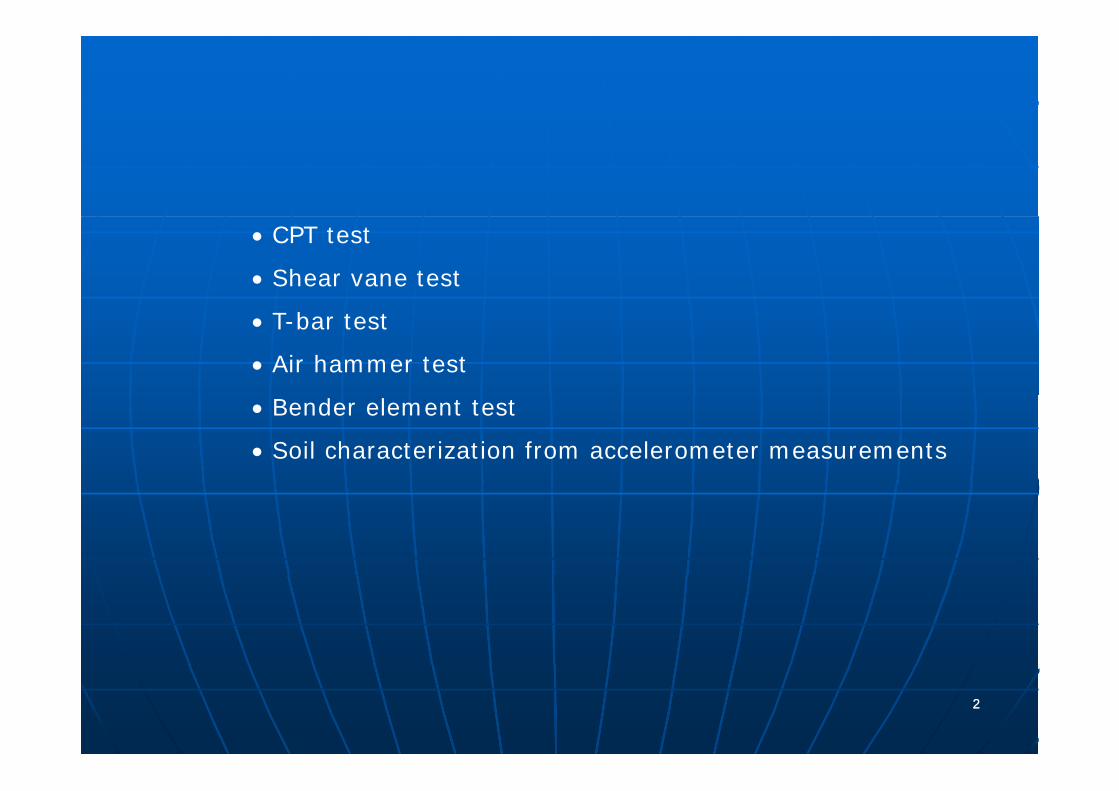
• CPT test
• Shear vane test
• T-bar test
• Air hammer test
• Bender element test
• Soil characterization from accelerometer measurements
22

Cone penetration test
⇒ Characteristics of CPT in centrifuge (Bolton et al 1999) : ⇒ Characteristics of CPT in centrifuge (Bolton et al., 1999) :
• repeatability of interlaboratory tests
• size effect B/d50 (in sand)
• side boundary effect S/B
• Initial penetration Δz/B effect - interface effect
i i f i f⇒ Determination of specimen parameters from CPT (Robertson & Campanella, 1983):
• soil strength
• deformation modulus /Vsdeformation modulus /Vs
• liquefaction potential
33

Cone penetration test
2 main objectives: - check the uniformity reproducibility of the specimen2 main objectives: - check the uniformity, reproducibility of the specimen
- obtained an indirect characteristic profile
Hydraulic CPT Electric CPT
At the prototype scale : Ø 38 mm ⇒ scaling of the cone penetrometer can not be achieved
44
Most of the miniature CPT : Ø around 10 mm (IFSTTAR 12 mm)

Cone penetration test • Reproducibility of interlaboratory tests (sand)• Reproducibility of interlaboratory tests (sand)
European Program of Improvement in centrifuging (EPIC)
Normalized cone Normalized cone
resistance Qh
Z
Variation within a ± 10 % band width
lize
d d
ep
tN
orm
a
(Bolton et al 1999)
55
(Bolton et al., 1999)
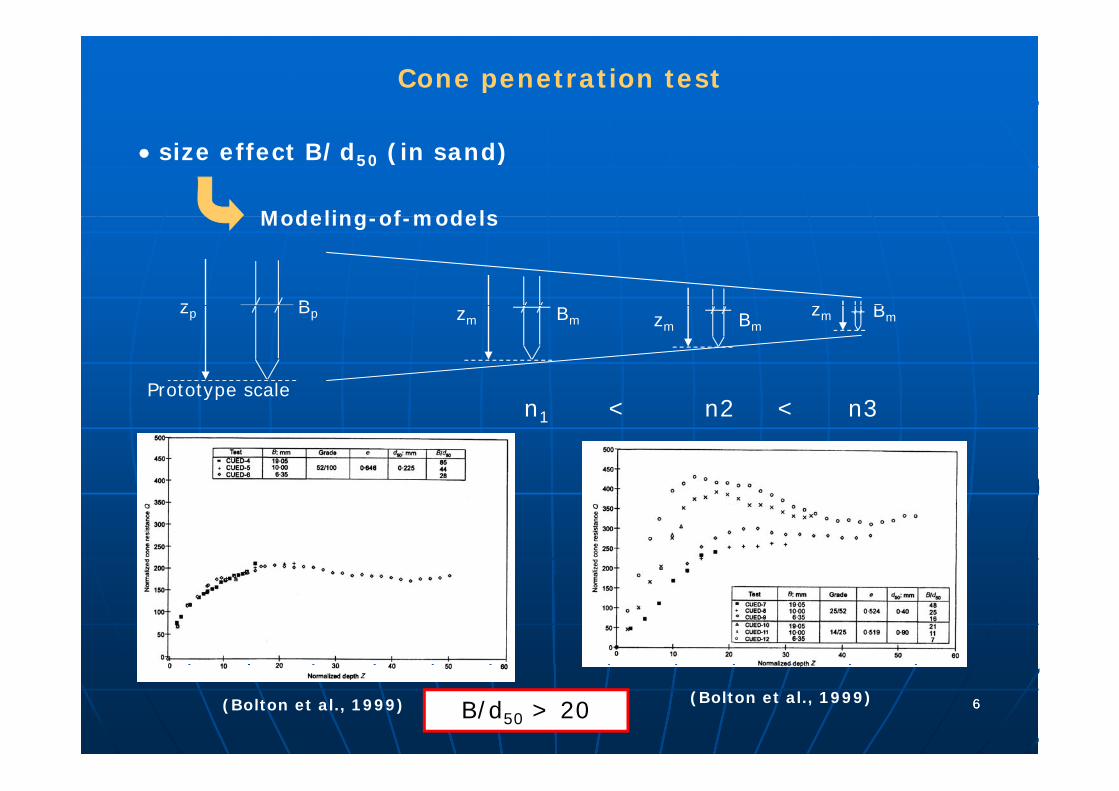
Cone penetration test
• size effect B/d50 (in sand)
Modeling of modelsModeling-of-models
z B z Bzm Bm
Prototype scale
zp Bp zm Bmzm Bm
Prototype scalen1 < n2 < n3
66B/d50 > 20(Bolton et al., 1999) (Bolton et al., 1999)

Cone penetration test
• side boundary effect S/B (sand)
(Bolton et al., 1999)
77At least 10B away from any hard boundary
(Bolton et al., 1999)

Cone penetration test
• Initial penetration Δz/B effect - Interfaces effect (sand)
- Boundary fringe 10B where Q increases with depth like shallow foundation (Bolton et al., 1999)
- Depending on relative density, boundary fring may lie between 5B
( , )
Normalized cone boundary fring may lie between 5B and 20B (Gui & Bolton)resistance Q
dep
th Z
No
rmali
zed
88(Bolton et al., 1999)(Gui & Bolton, 1998)

Cone penetration test
• Initial penetration Δz/B effect - Interfaces effect
(Gui & Bolton, 1998)
99

Cone penetration test
• Shear strength in sand (Rayhani & El Naggar, 2008)
1010(Robertson & Campanella, 1983)

Cone penetration test
• Shear strength in clay
Correlation between CPT tests and shear t t f h l
Empirical relationshipvane test for each clay
uc ASq =
1000
1200
c
vcu N
qS σ−=
800
1000
inte
qc
(kPa
)
Nc : cone factor that depends on OCR
400
600
resi
stan
ce e
n po
i
conteneur A (melange kaolinite-chaux a 1%)
0 10 20 30 40 50 60 70 80cohesion non drainee Su (kPa)
0
200 regression linéaire : Y= 17.33 X
Conteneur B (melange kaolinite-chaux a 2%)
regresion lineaire : Y= 17.04 X
rapport conventionnel qc/Su : 18.5
(Rault 2009)
1111
cohesion non drainee Su (kPa)
Determination d'une relation Qc et SuEssais preliminaires a 1G - fevrier & mars 2009
massifs A (KC01 (1%)) & B (KC02 (2%)] (conteneurs diametre 300mm) SOLCYP01.grf
(Rault, 2009)

Cone penetration test
• Deformation modulus (E, Gmax)
(Rayhani & El Naggar 2008)(Rayhani & El Naggar, 2008)
Around 10B
1212
Cone penetration test
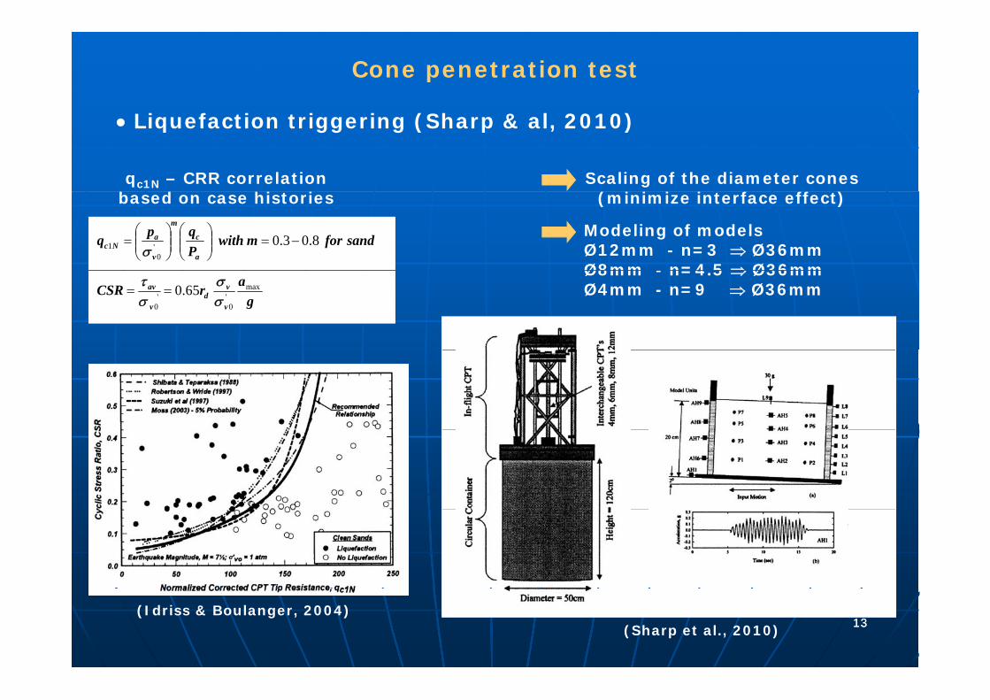
• Liquefaction triggering (Sharp & al, 2010)
qc1N – CRR correlation b d hi i
Scaling of the diameter cones ( i i i i f ff )based on case histories (minimize interface effect)
Modeling of modelsØ12mm - n=3 ⇒ Ø36mmØ8mm - n=4 5 ⇒ Ø36mm
sandformwithPqpq
a
c
m
v
aNc 8.03.0'
01 −=⎟⎟
⎠
⎞⎜⎜⎝
⎛⎟⎟⎠
⎞⎜⎜⎝
⎛=
σØ8mm - n=4.5 ⇒ Ø36mmØ4mm - n=9 ⇒ Ø36mm
garCSR
v
vd
v
av max'0
'0
65.0σσ
στ
==
1313(Idriss & Boulanger, 2004)
(Sharp et al., 2010)

Cone penetration test
• Liquefaction triggering (Sharp & al, 2010)
- Modeling of models - Good correlation between qc1N and Lateral displacement & thickness of liquefied layer
(Sharp & al, 2010)(Sharp & al 2010)
- Results consistent with the field liquefaction chart based on case histories(Sharp & al, 2010)
(Sharp & al, 2010)
1414

Shear vane test
• Determination of Su for soft soil
⇒Determination of the Su value
kMS t
u =
Drawback : discrete values
Advantage : peack value and strain softening behaviour
⇒ Parameters that affect Su(D i t l 1989 & W t t l 1998)
g
(Rault, 2008)(Davis et al., 1989)
(Davis et al, 1989 & Watson et al., 1998)
-delay between insertion and rotation
-rate of rotation
-vane geometry
⇒ Centrifuge test : variation of σ’ along the vane heigth
1515
of σ v along the vane heigth

Shear vane test
• Determination of Su for soft soil
Correlation with CPT – 1g test(if D i l 1989)
Infligth determination of cu(W l 1998)(ifsttar – Davis et al., 1989) (Watson et al. 1998)
NF P94-072 (1995) NF P94-112 (1991)
vane geometry
NF ⇒ aspect ratio h/d=2
Centrifuge modeling ⇒ variation of σv’ along H ⇒ decrease of the aspect ratio
Infligth test(Watson et al. 1998)
1g test(Davis et al. 1989)
Vane H (mm)
D (mm)
H/D
A 28 19 1.47
Vane H (mm)
D mm)
H/D
A 10 15 0 67
A 28 19 1.47
B 14 18 0.78
C 14 27 0.52
D 14 36 0.39
1616
A 10 15 0.67
B 10 10 1
C 15 10 1.5

Shear vane test
• Determination of Su for soft soil
Correlation with CPT – 1g test(if D i l 1989)
Infligth determination of cu(W l 1998)(ifsttar – Davis et al., 1989) (Watson et al. 1998)
NF P94-072 (1995) NF P94-112 (1991)
Rate of rotation (linked to the vane geometry) : undrained conditions
Both NF : 18°/min ⇒ rate of shearing at the end of the blade 0.026-0.04mm/s and 0.18mm/s
Centrifuge modelling ⇒ scaling factor for dynamic time and diffusion time
04.002.02 totc
T fv ≤=(Davis et al., 1989) Tf : time to failure0.00.02 to
D
Vane H (mm) D (mm) Shear rate
Cv consolidation coefficient
Vane H (mm) D (mm) Shear rate (mm/s)
(mm/s)
B 14 18 0.18
(Davis et al., 1989)
A 10 10 0.09
B 13 13 0.11
C 20 20 0.17
D 30 30 0 26
1717
D 30 30 0.26
E 40 40 0.34
IFSTTAR
Shear vane test
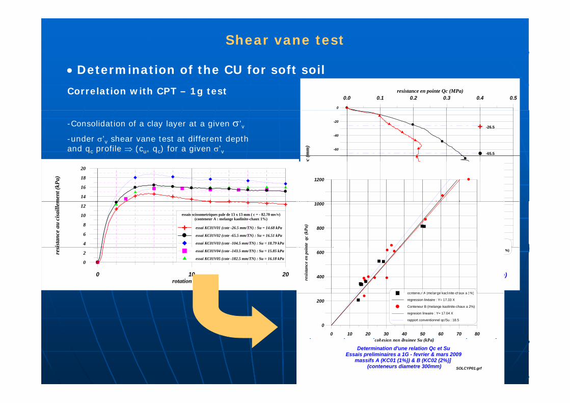
• Determination of the CU for soft soil
Correlation with CPT – 1g test0.0 0.1 0.2 0.3 0.4 0.5
resistance en pointe Qc (MPa)
0
-60
-40
-20
(mm
)
-26.5
-65.5
-Consolidation of a clay layer at a given σ’v-under σ’v shear vane test at different depth and qc profile ⇒ (cu, qc) for a given σ’v
14
16
18
20
men
t (kP
a)
-120
-100
-80
ofon
deur
mod
ele
zpc
(
-104.51200
4
6
8
10
12
ista
nce
au c
isai
llem
essais scissometriques pale de 13 x 13 mm ( c = - 82.70 mv/v)(conteneur A : melange kaolinite-chaux 1%)
essai KC01V01 (cote -26.5 mm/TN) : Su = 14.68 kPa
essai KC01V02 (cote -65.5 mm/TN) : Su = 16.51 kPa
essai KC01V03 (cote -104.5 mm/TN) : Su = 18.79 kPa-200
-180
-160
-140prof
-143.5
-182.5profil penetrometrique PA01(kaolinite pure) - contrainte 102 kPa (W = 39.5 %)
800
1000
nte
qc
(kPa
)
0 10 20rotation (degre)
0
2res essai KC01V04 (cote -143.5 mm/TN) : Su = 15.85 kPa
essai KC01V05 (cote -182.5 mm/TN) : Su = 16.18 kPa Determination de Qc et Su(Essais preliminaires a 1G - 16.03.2009)
Conteneurs A (KC01) & B (KC02) - (diametre 300mm)
200profil penetrometrique KC01P01 (melange kaolinite-chaux a 1%) - contrainte 119 kPa (W = 72.2 %)
400
600
resi
stan
ce e
n po
in
conteneur A (melange kaolinite chaux a 1%)
0 10 20 30 40 50 60 70 80h i d i S (kP )
0
200
conteneur A (melange kaolinite-chaux a 1%)
regression linéaire : Y= 17.33 X
Conteneur B (melange kaolinite-chaux a 2%)
regresion lineaire : Y= 17.04 X
rapport conventionnel qc/Su : 18.5
1818
cohesion non drainee Su (kPa)
Determination d'une relation Qc et SuEssais preliminaires a 1G - fevrier & mars 2009
massifs A (KC01 (1%)) & B (KC02 (2%)] (conteneurs diametre 300mm) SOLCYP01.grf

T-bar test
D b k f CPT d h t t (St t & R d l h 1991)Drawbacks of CPT and shear vane test (Stewart & Randolph, 1991)
- CPT : interpretation largely based on empirical relationships
- shear vane test : physical size VS sample height
T-bar : continuous profile – results can be analysed directly in terms of yield shear strength
- relative rough cylindrical surface- relative rough cylindrical surface
- smooth end surface
- rate of penetration :few mm/s
- penetration resistance measured just behind the T-barpenetration resistance measured just behind the T bar
- hypothesis : full closure of the soil behind the cylinder
- Theory plastic solution for limiting pressure acting on a cylinder moving laterally through cohesive soil (Randolph & Houlsby 1984)Houlsby, 1984)
dSNP ub=
(Stewart & Randolph, 1991)P: force per unit length acting on the cylinder
D: diameter
N : bar factor (recommended value 10 5 Randolph &
1919
Nb: bar factor (recommended value 10.5 Randolph & Houlsby, 1984)

T-bar test
2020
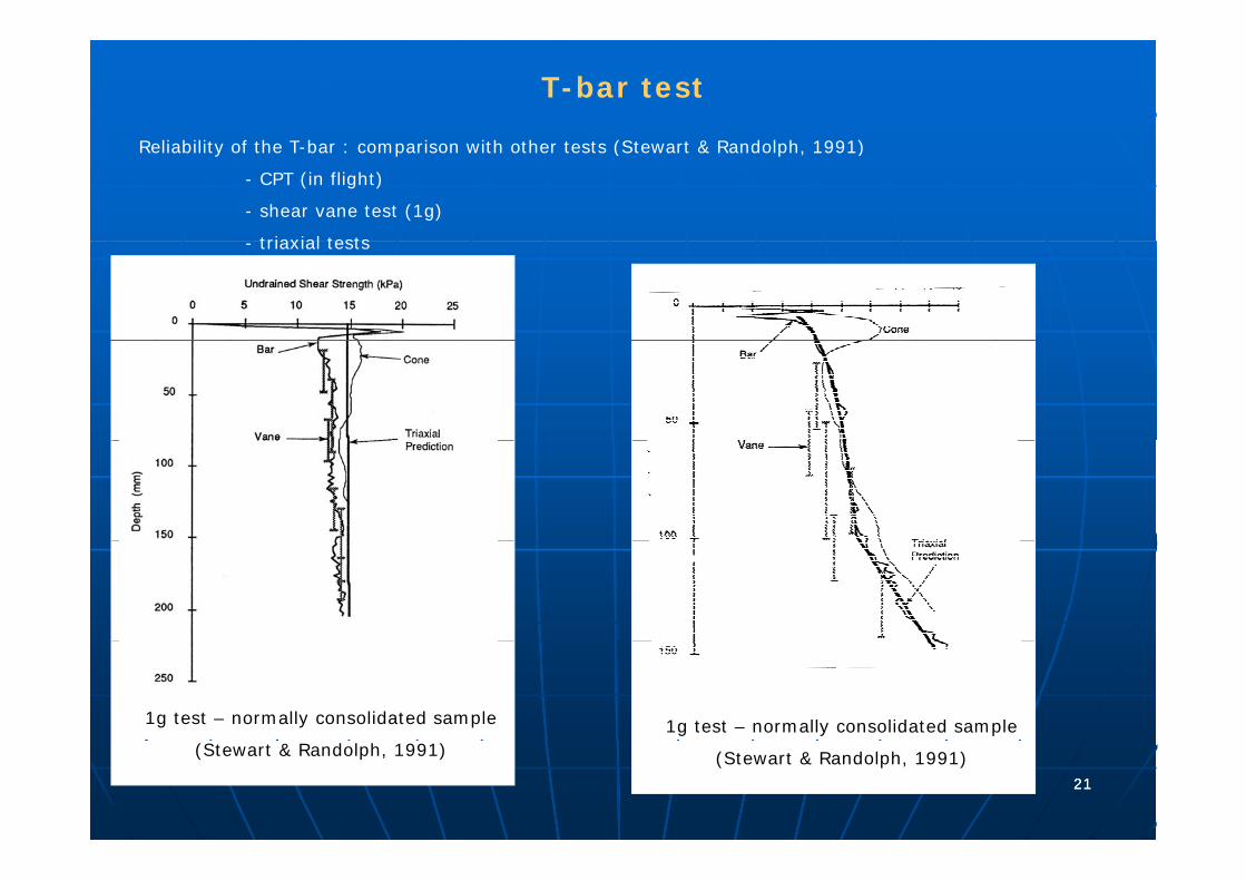
T-bar test
R li bilit f th T b i ith th t t (St t & R d l h 1991)Reliability of the T-bar : comparison with other tests (Stewart & Randolph, 1991)
- CPT (in flight)
- shear vane test (1g)
triaxial tests- triaxial tests
1g test – normally consolidated sample1g test – normally consolidated sample
2121
(Stewart & Randolph, 1991)(Stewart & Randolph, 1991)

Air-hammer test
• Shear wave velocity
(Arulnathan et al., 2000 ; Ghosh & Madabhushi, 2002)
Air hammer AccelerometerAir hammer Accelerometer
(Arulnathan et al., 2000) (Ghosh & Madabhushi, 2002)
-requiered properties
- well-define and repeatable shear wave pulsep p
- usefull range of frequency
- magnitude of the soil distorsion
2222

Air-hammer test
• Shear wave velocity
Cambridge Davis
Hollow cylinder Brass 42mm long Aluminium 47mm longHollow cylinder Brass 42mm long Aluminium 47mm long
Piston Teflon 19mm long Teflon 25mm long
valve 3 ways solenoid 4 ways solenoidvalve 3 ways solenoid 4 ways solenoid
Outer surface of the cylinder Sand (glued) Sand (glued)
(Arulnathan et al., 2000)(Ghosh & Madabhushi, 2002)
2323

Air-hammer test
• Shear wave velocity
frequency content
Vs wavelength /distance between accelerometer as small a possible (Arulnathan et al., 2000)
(Arulnathan et al., 2000)
Increase of the sampling frequency
λ (cm) < d
d λ Vs
Model scale1 2 3 4
150 30kHz 15kHz 10kHz 7 5kHzacc1
acc2
2424Vs (m/s)
150 30kHz 15kHz 10kHz 7.5kHz
300 60kHz 30kHz 20kHz 15kHz
acc1

Air-hammer test
• Shear wave velocity
Amplitude – shear strain level
Gmax ⇒ γ ≅ 10-6 to 10-5
(Arulnathan et al 2000)(Ghosh & Madabhushi 2002) (Arulnathan et al., 2000)(Ghosh & Madabhushi, 2002)
γ Estimated from the double integration of the
accelerometer measurements
γ Estimated from maximum acceleration, a0, and hypothesis of
an equivalent sine wave, ωaccelerometer measurements a equ a e t s e a e, ω
Maximum displacement
20
ωaMaximum distorsion
⎟⎞
⎜⎛ −∫∫ ∫∫ 12 accacc
a02Maximum distorsion⎟
⎟
⎠⎜⎜
⎝ −= ∫∫ ∫∫
12max max
accacc zzγ
2525ωπ sV

Bender element tests
• Bender element = piezoelectric transducer
Receiver : series bender
Transmitter: parallel bender
(Brandenberg et al., 2006)
• Configuration of bender element system
Wave generatorOscilloscope
(data acquisition)
amplifier amplifier
2626transmitter receiver
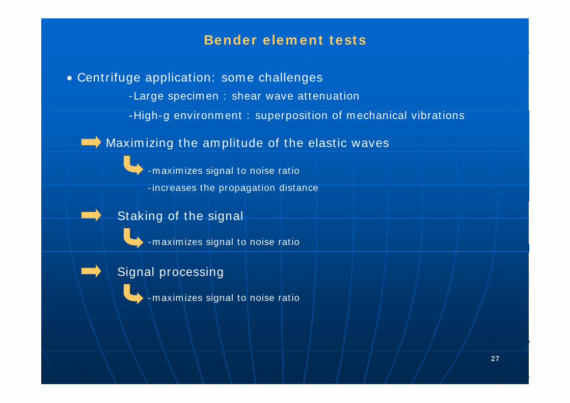
Bender element tests
• Centrifuge application: some challenges-Large specimen : shear wave attenuation
-High-g environment : superposition of mechanical vibrations
Maximizing the amplitude of the elastic waves
-maximizes signal to noise ratio
-increases the propagation distance
Staking of the signal
-maximizes signal to noise ratio
Signal processing
-maximizes signal to noise ratio
2727
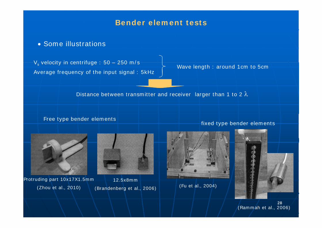
Bender element tests
• Some illustrations
V velocity in centrifuge : 50 250 m/sVs velocity in centrifuge : 50 – 250 m/s
Average frequency of the input signal : 5kHzWave length : around 1cm to 5cm
Distance between transmitter and receiver larger than 1 to 2 λ
Free type bender elementsfixed type bender elements
Protruding part 10x17X1.5mm
(Zhou et al., 2010)
12.5x8mm
(Brandenberg et al., 2006) (Fu et al., 2004)
2828(Rammah et al., 2006)

Bender element tests
• Liquefaction triggering Liu G. (2009)
Cross section viewBender element ⇒ Vs(z)
( ) 5.0'5.0
02
max 321
197.23230
vK
ee
G σ⎟⎟⎠
⎞⎜⎜⎝
⎛ ++
−=
(Hardin & Drnevich, 1972)
2max sVG ρ=
25.0
'1 ⎟⎟⎠
⎞⎜⎜⎝
⎛=
vss
PaVVσ ⎠⎝
Acceleration measurements during earthquake ⇒ amax
garCSR v
dav max
'' 65.0σσ
στ
==
(Seed & Idriss, 1971) (Liao & Whitman, 1986)
CSRrd (z)gvv 00 σσ
Pore pressure measurements during earthquake ⇒ Δu
Top view'0vu σ=Δ
Liquefaction
or not
2929Liu G. (2009)

Bender element tests
• Liquefaction triggering Liu G. (2009)
Liu G. (2009) Liu G. (2009)
3030

Soil characterisation from accelerometer measurements
(Zeghal et al., 1995)
One dimensional shear beam idealisationy
• τ-γ loops , G(γ )/Gmax , β(γ)/ βmax
One dimensional shear beam idealisation
( ) ( )dztzutzz
∫= ,, &&ρτ
( ) 0,0 =tτ ( ) HutHu &&&& =,
zH
Soil column with a vertical array of accelerometers
( ) ( ) zzz ∫0 ,, ρ
• U(0,t) : linear fit from the top pair of accelerometers
( )223
2321 0 z
zzuuuu −
−−
+=&&&&
&&&&
• Determination of (z t)• Determination of τ (z,t)
Few accelerometers
limited amplification/attenuation h
many accelerometers
significant amplification/attenuation h
(Z h l t l 1995)
phenomena phenomena
Trapezoidal integrationUse on the surface acceleration
3131
(Zeghal et al., 1995)(Zhegal et al., 1995)(Zhegal et al., 1994)
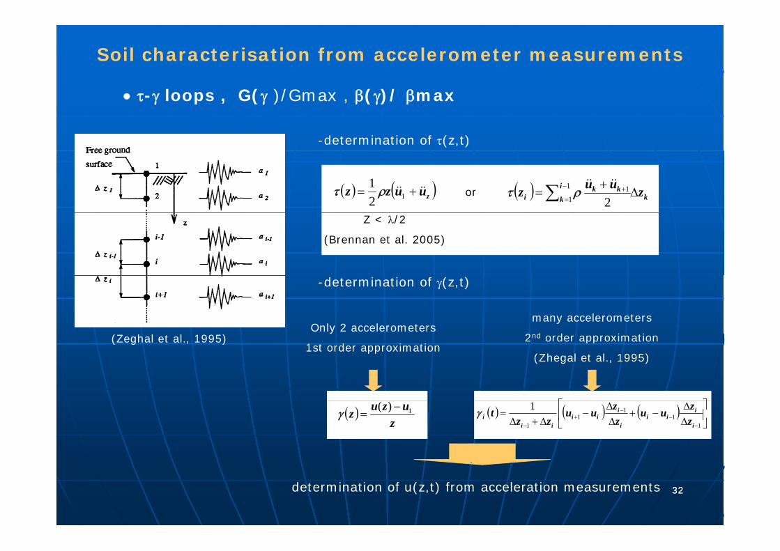
Soil characterisation from accelerometer measurements
• τ-γ loops , G(γ )/Gmax , β(γ)/ βmax
-determination of τ(z,t)
( ) ( )zuuzz &&&& += 121 ρτ ( ) k
i
kkk
i zuuz Δ+
=∑ −
=+1
11
2&&&&
ρτor
Z < λ/2
(Brennan et al. 2005)
(Zeghal et al 1995)
-determination of γ(z,t)
Only 2 accelerometersmany accelerometers
2nd order approximation(Zeghal et al., 1995)1st order approximation
2nd order approximation
(Zhegal et al., 1995)
⎤⎡( )z
uzuz 1)( −=γ ( ) ( ) ( ) ⎥
⎦
⎤⎢⎣
⎡ΔΔ
−+ΔΔ
−Δ+Δ
=−
−−
+− 1
11
11
1
i
iii
i
iii
iii z
zuuzzuu
zztγ
3232determination of u(z,t) from acceleration measurements

Soil characterisation from accelerometer measurements
• τ-γ loops , G(γ )/Gmax , β(γ)/ βmax
- determination of u(z,t) from acceleration measurements
Data processing : integration + filteringEffect of direct integration
Appropriate filter:
-frequency range of interest
-non dispersive filter or dispersive filter (limited dispersion in the frequency range of interest)
-adequacy between the required adequacy between the required sharpness of the pass band filter and the filter order
-filtfilt function in Matlab© to avoid phase h fshift
3333

Soil characterisation from accelerometer measurements
• τ-γ loops , G(γ )/Gmax , β(γ)/ βmax
Importance of the paccelerometers properties
(phase lag)
3434

Soil characterisation from accelerometer measurements
• τ-γ loops , G(γ )/Gmax , β(γ)/ βmax
loopAβ =
triangleAπβ
4=
γτ
ΔΔ
=G
(Hardin et al. 1972)
3535

Soil characterisation from accelerometer measurements
Importance of the frequency range of the pass-band filter
• τ-γ loops , G(γ )/Gmax , β(γ)/ βmax
Frequency range :
20-450Hz Frequency range :
20-70 Hz
3636
(Brennan et al., 2005)

Soil characterisation from accelerometer measurements
• τ-γ loops , G(γ )/Gmax , β(γ)/ βmax
3737(Rayhani & El Naggar, 2007) (Brennan et al., 2005)