SANDIA REPORT SAND2012-7328 Unlimited Release September 2012

Continuous Reliability Enhancement for Wind (CREW) Database: Wind Plant Reliability Benchmark Valerie A. Peters, Alistair B. Ogilvie, Cody R. Bond Prepared by Sandia National Laboratories Albuquerque, New Mexico 87185 and Livermore, California 94550

Sandia National Laboratories is a multi-program laboratory managed and operated by Sandia Corporation, a wholly owned subsidiary of Lockheed Martin Corporation, for the U.S. Department of Energy's National Nuclear Security Administration under contract DE-AC04-94AL85000. Approved for public release; further dissemination unlimited.

2

Issued by Sandia National Laboratories, operated for the United States Department of Energy by Sandia Corporation. NOTICE: This report was prepared as an account of work sponsored by an agency of the United States Government. Neither the United States Government, nor any agency thereof, nor any of their employees, nor any of their contractors, subcontractors, or their employees, make any warranty, express or implied, or assume any legal liability or responsibility for the accuracy, completeness, or usefulness of any information, apparatus, product, or process disclosed, or represent that its use would not infringe privately owned rights. Reference herein to any specific commercial product, process, or service by trade name, trademark, manufacturer, or otherwise, does not necessarily constitute or imply its endorsement, recommendation, or favoring by the United States Government, any agency thereof, or any of their contractors or subcontractors. The views and opinions expressed herein do not necessarily state or reflect those of the United States Government, any agency thereof, or any of their contractors. Printed in the United States of America. This report has been reproduced directly from the best available copy. Available to DOE and DOE contractors from U.S. Department of Energy Office of Scientific and Technical Information P.O. Box 62 Oak Ridge, TN 37831 Telephone: (865) 576-8401 Facsimile: (865) 576-5728 E-Mail: reports@adonis.osti.gov Online ordering: http://www.osti.gov/bridge Available to the public from U.S. Department of Commerce National Technical Information Service 5285 Port Royal Rd. Springfield, VA 22161 Telephone: (800) 553-6847 Facsimile: (703) 605-6900 E-Mail: orders@ntis.fedworld.gov Online order: http://www.ntis.gov/help/ordermethods.asp?loc=7-4-0#online

3

SAND2012-7328 Unlimited Release September 2012

Continuous Reliability Enhancement for

Wind (CREW) Database: Wind Plant Reliability Benchmark

Valerie A. Peters, Alistair B. Ogilvie, Cody R. Bond

Wind Energy Technologies Sandia National Laboratories

P.O. Box 5800, MS 1124 Albuquerque, New Mexico 87185

Abstract

To benchmark the current U.S. wind turbine fleet reliability performance and identify the major contributors to component-level failures and other downtime events, the Department of Energy (DOE) funded the development of the Continuous Reliability Enhancement for Wind (CREW) database by Sandia National Laboratories. This report is the second annual Wind Plant Reliability Benchmark, to publically report on CREW findings for the entire wind industry.

The CREW database uses both high resolution Supervisory Control and Data Acquisition (SCADA) data from operating plants and Strategic Power Systems’ (SPS) ORAPWind® (Operational Reliability Analysis Program for Wind) data, which consists of downtime and reserve event records and daily summaries of Generating, Unavailable, and Reserve time for each turbine. Together, these data are used as inputs into CREW’s reliability modeling.

The results presented here include: the primary CREW Benchmark statistics (operational availability, utilization, capacity factor, mean time between events, and mean downtime); time accounting from an availability perspective; time accounting in terms of the combination of wind speed and generation levels; power curve analysis; and top system and component contributors to unavailability.

4

Acknowledgments This public Benchmark report is the second industry report to be issued under the Continuous Reliability Enhancement for Wind (CREW) national database project, with the first being published in October 2011. The CREW project is guided and funded by the Department of Energy, Energy Efficiency and Renewable Energy program office. Sandia National Laboratories would like to acknowledge the contributions of both Strategic Power Systems and the wind plant owner/operators who participated in the development of the CREW database as pilot partners. These partners include enXco Service Corporation, Shell WindEnergy Inc., Xcel Energy, and Wind Capital Group. Data gathered from these and other individual partners is proprietary and is only used in an aggregated manner, in order to protect data privacy.

5

Contents

Acknowledgments........................................................................................................................... 4 Contents .......................................................................................................................................... 5 Figures............................................................................................................................................. 6 Tables .............................................................................................................................................. 6 Executive Summary ........................................................................................................................ 7 1.0 Introduction ............................................................................................................................... 9 

1.1.  Wind Energy at Sandia National Laboratories ............................................................... 9 1.2.  CREW Data .................................................................................................................. 10 

1.2.1.  SCADA Data .......................................................................................................... 11 1.2.2.  ORAPWind® Data ................................................................................................. 11 

2.0 Wind Plant Reliability Benchmark ......................................................................................... 12 2.1.  Fleet Representation ...................................................................................................... 12 2.2.  Results and Discussion ................................................................................................. 13 

2.2.1.  Other Benchmarks .................................................................................................. 13 2.2.2.  Known Time ........................................................................................................... 14 2.2.3.  Availability Time Accounting ................................................................................ 15 2.2.4.  Wind Speed and Generation Time Accounting ...................................................... 15 2.2.5.  Power Curve............................................................................................................ 17 2.2.6.  Wind Turbine Unavailability Contributors ............................................................. 18 

3.0 Observations ........................................................................................................................... 21 Appendix A: Methodology and Calculations ............................................................................... 22 Appendix B: Nomenclature .......................................................................................................... 30 

6

Figures

Figure 1. Availability Time Accounting – Known Time Only. ...................................................... 8 Figure 2. Event Frequency versus Downtime. ................................................................................ 8 Figure 3. ORAPWind® Data Transfer Process to CREW. .......................................................... 10 Figure 4. Improvements in Known Time. ..................................................................................... 14 Figure 5. Availability Time Accounting – All Time Accounted. ................................................. 14 Figure 6. Availability Time Accounting – Known Time Only. .................................................... 15 Figure 7. Wind Speed and Generation Time Accounting – Known Time Only ........................... 16 Figure 8. Power Curve .................................................................................................................. 17 Figure 9. Unavailability Contributors, Top 10 Systems. .............................................................. 18 Figure 10. Unavailability Contributors, System Event Frequency and Downtime. ..................... 19 Figure 11. Unavailability Contributors, Top 10 Component + Event Type contributors. ............ 20 Figure 12. Equipment Breakdown Structure Excerpt. .................................................................. 29 

Tables

Table 1. CREW Fleet Metrics. ........................................................................................................ 7 Table 2. Example of ORAPWind® Events. ................................................................................. 11 Table 3. CREW Database Metadata. ............................................................................................ 12 Table 4. CREW Fleet Metrics. ...................................................................................................... 13 Table 5: Time Accounting, Wind Speed and Generation, Known Time Only. ............................ 16 Table 6. Wind Plant Reliability Model, System Detail. ............................................................... 19 Table 7. Wind Speed Categories. .................................................................................................. 26 Table 8. Power Generation Categories. ........................................................................................ 26 

7

Executive Summary To benchmark the current U.S. wind turbine fleet reliability performance and identify the major contributors to component-level failures and other downtime events, the Department of Energy (DOE) funded the development of the Continuous Reliability Enhancement for Wind (CREW) database by Sandia National Laboratories (Sandia). This report is the second annual Wind Plant Reliability Benchmark, to publically report on CREW findings for the entire wind industry.

The CREW database uses two primary types of data, which are used to perform subsequent calculations and provide the foundation for reliability reporting. The first type of data is high resolution Supervisory Control and Data Acquisition (SCADA) data, collected at high frequency from operating plants. CREW analysis uses the high frequency data and also uses ten minute summaries of this data. The second type of data is from Strategic Power Systems’ (SPS) Operational Reliability Analysis Program for Wind (ORAPWind®). This data consists of downtime and reserve event records and daily summaries of Generating, Unavailable, and Reserve time for each turbine.

Results at a Glance

The five key CREW metrics are summarized in Table 1. The metrics show improvements in all categories compared to the 2011 Benchmark report.

Table 1. CREW Fleet Metrics. 2012 Benchmark 2011 Benchmark Operational Availability 97.0% 94.8%Utilization (Generating Factor) 82.7% 78.5% Capacity Factor 36.0% 33.4% MTBE (Mean Time Between Events) 36 hrs 28 hrs Mean Downtime 1.6 hrs 2.5 hrs

A graphic summary of how a typical CREW turbine spends its time is provided in Figure 1. For each main turbine system, Figure 2 shows the Annual Number of Events per Year per Turbine, which is the expected number of events per turbine per calendar year, and it also shows the Mean Downtime per Event. Note that the generic system “Wind Turbine (Other)” dominates the frequency and downtime. This is due to a large number of SCADA events that do not have adequate detail to be assigned to a specific system.

8

Figure 1. Availability Time Accounting – Known Time Only.

Figure 2. Event Frequency versus Downtime.

9

1.0 Introduction The “20% Wind Energy by 2030” report1, published in 2008 by a DOE collaborative, specifically discusses industry risk from lower-than-expected reliability and increasing operations and maintenance costs. To benchmark the current U.S. wind turbine fleet reliability performance and identify the major contributors to component-level failures and other downtime events, DOE funded Sandia to develop the CREW database. This national reliability database of wind plant operating data enables reliability analysis, with the following six key objectives:

Benchmark reliability performance

Track operating performance at a system-to-component level

Characterize issues and identify technology improvement opportunities

Protect proprietary information

Enable operations and maintenance cost reduction

Increase confidence from the financial sector and policy makers

The goal of this Wind Plant Reliability Benchmark is to publically report on Sandia’s reliability findings for the entire wind industry. Previous Benchmarks can be found on Sandia’s website at http://energy.sandia.gov/crewbenchmark.

1.1. Wind Energy at Sandia National Laboratories Our highest goal is to become the laboratory the United States turns to first for innovative, science-based systems-engineering solutions to the most challenging problems that threaten peace and freedom for our nation and the globe.

Sandia National Laboratories Strategic Plan2

The U.S. Congress made Sandia National Laboratories a DOE National Laboratory in 1979, but Sandia’s history goes all the way back to 1945 and World War II’s Manhattan Project2. Changing with the nation’s security needs, Sandia currently has four key mission areas: Energy, Climate, and Infrastructure Security (the mission area for Renewable Energy); Nuclear Weapons; Defense Systems and Assessments; and International, Homeland, and Nuclear Security3.

1 U.S. Department of Energy (DOE), Energy Efficiency and Renewable Energy. “20% Wind Energy by 2030. Increasing Wind Energy’s Contribution to U.S. Electricity Supply.” DOE/GO-102008-2567. Springfield, VA. Jul 2008. Accessed on Aug 14 2012 from http://www.eere.energy.gov/wind/pdfs/42864.pdf 2 U.S. DOE, Sandia National Laboratories. “Sandia 2008” (Annual Report). SAND-2008-2628P. Albuquerque, NM. 2008. Accessed on Jul 30 2012 from http://www.sandia.gov/news/publications/annual_report/_assets/documents/ar2008_SAND-2008-2682P.pdf 3 U.S. DOE, Sandia National Laboratories. “National Security Missions.” Accessed on Jul 30 2012 from http://www.sandia.gov/missions/index.html

10

The CREW project is managed by Sandia’s Wind Energy Technologies department, which traces its roots to the energy crisis of the mid-1970s. The original focus was on vertical axis wind turbines, but transitioned to wind turbine blades in the early 1990s. With the ever-present goal of increasing the viability of wind technology, Sandia’s current projects focus on applied research to improve wind plant performance, reliability, and cost of energy. Sandia’s areas of expertise include wind-turbine blade design, manufacturing, and system reliability4.

1.2. CREW Data For the CREW project, Sandia partners with SPS whose ORAPWind® system collects real-time data from partner plants. The majority of CREW data originates from ORAPWind® and its automated data collection, going through an SPS transformation process before being loaded into CREW. As Figure 3 illustrates, Sandia uses both the raw SCADA data and transformed events data from ORAPWind®. In addition to the data from ORAPWind®, a smaller portion of the CREW data comes directly from wind plant owner/operators, usually in the form of ten minute SCADA summaries (see Section 1.2.1 “SCADA Data”). All relevant data is used in each piece of the analysis, though a given graph or metric may not include every plant in the dataset.

Figure 3. ORAPWind® Data Transfer Process to CREW.

The guiding principle for CREW data and reporting is that data gathered from individual partners is proprietary and will only be shared when it is sufficiently masked or aggregated, to protect data privacy. Due to a large volume of requests and limited funding, Sandia cannot provide customized aggregated data outside the DOE’s Energy Efficiency and Renewable Energy (EERE) program. For requests outside EERE, please see SPS’ website at http://orapwind.spsinc.com. Past Sandia wind plant reliability publications are located at http://energy.sandia.gov/?page_id=3057#WPR.

4 U.S. DOE, Sandia National Laboratories. “Wind Energy.” Accessed on Jul 30 2012 from http://energy.sandia.gov/?page_id=344

11

1.2.1. SCADA Data High Resolution SCADA Data: SPS’ automated data collection process gathers observations recorded by the SCADA systems at their partners’ wind plants. This data is collected at high frequency (approximately every two to ten seconds) by the ORAPWind® tool, transferred to SPS, and then transferred to Sandia. Data points cover the “heartbeat” of the turbine (e.g., operating state, rotor speed) and environmental conditions measured by the turbines and the meteorological (met) towers (e.g., wind speed, air pressure, ambient air temperature, etc.). Ten Minute SCADA Summaries: In addition to storing the high resolution SCADA data, CREW also uses it to create ten minute summaries. These summaries consist of ten minute minimums, maximums, averages, and standard deviations for each numeric data stream (e.g., wind speed) and a statistical mode (most common observation) for discrete values (e.g. turbine state).

1.2.2. ORAPWind® Data Events: The ORAPWind® tool summarizes the SCADA data into downtime and reserve events, covering any time that any turbine is not generating. Reserve events capture when the turbine is available to generate, but not generating due to external circumstances; these are NOT counted by the CREW team as “downtime events.” Each event consists of a start and end date/time, affected turbine, and description of the problem. This description includes a general event type (e.g., Reserve Shutdown or Unscheduled Maintenance) and affected component from SPS’ Equipment Breakdown Structure (EBS) (e.g., Rotor Blade or Stator - Electric Generator). Table 2 shows key data fields for two hypothetical ORAPWind® events.

Table 2. Example of ORAPWind® Events.

Turbine ID

Event ID

Event Type Begin Date

End Date

EBS Component

Outage Mechanism

123 5688 Forced Outage Automatic Trip

1/3/11 15:16

1/4/11 11:34

Pitch Controller

Erratic (electrical)

123 5678 Reserve Shutdown

1/1/11 01:23

1/1/11 04:56

Yaw Cable Twist Counter

Position, Incorrect

Operational Records: ORAPWind® also summarizes the SCADA data by reporting on the amount of time each turbine spends in various states. For each 24 hour day, the total time in each state is calculated. The main states of interest are: Contact Hours (time the unit is generating), Reserve Hours (time the unit is available to generate, but is not generating), and Unavailable Hours (time the unit is not available to generate). If full data has been collected, the sum of Contact, Reserve, and Unavailable hours will equal 24 hours each day.

12

2.0 Wind Plant Reliability Benchmark

2.1. Fleet Representation The CREW results presented are considered “directional” by the authors. Early CREW reports are based heavily on data collected during the development phase of the project and the database does not yet represent a significant portion of the U.S. wind turbine fleet, thus it would be premature to consider the results here fully “actionable.” However, the data quality and operations breadth provided by early data partners has generated a dataset that provides a useful initial view of the U.S. fleet’s operational and reliability performance.

The CREW database continues to grow, in terms of new plants, new technologies, and more information from existing partners. Table 3 summarizes the metadata for the CREW database, capturing the depth and breadth quantitatively. The current data covers 3 turbine manufacturers, 6 turbine models, and over 180,000 turbine-days. Future reporting will be based on even larger datasets, with an eventual goal of representing 10% of the large, modern U.S. wind fleet’s performance. CREW currently represents approximately 3% of the large, modern U.S. wind turbines. The scope of the CREW database includes wind turbines that are at or above 1 megawatt (MW) in size, from plants with at least 10 turbines.

Table 3. CREW Database Metadata. # Plants 10 # Turbines 800-900 # Megawatts 1300-1400 # Manufacturers 3 # Turbine Models 6 # Turbine-Days, Known Time5 180,000

CREW’s ability to represent the U.S. wind fleet’s performance is based on its volume and variety of operating data. All U.S. wind plant owners, operators, and original equipment manufacturers (OEMs) are invited to participate. For more information, please contact Alistair Ogilvie, Sandia CREW Project Lead at (505) 844-0919 or Alistair.Ogilvie@sandia.gov.

5 All analyses use the known time only, unless unknown time is specifically mentioned.

13

2.2. Results and Discussion The five key CREW metrics are summarized in Table 4. The metrics have all improved since the 2011 Benchmark publication. While actual performance improvement is likely a significant contributor, this may also be due to a variety of other factors that include the presence of all four seasons in this Benchmark and improved data quality.

Table 4. CREW Fleet Metrics.

2012 Benchmark 2011 Benchmark Operational Availability 97.0% 94.8%Utilization (Generating Factor) 82.7% 78.5% Capacity Factor 36.0% 33.4% MTBE6 (Mean Time Between Events) 35 hrs 28 hrs Mean Downtime6 1.6 hrs 2.5 hrs

2.2.1. Other Benchmarks There was reasonably good alignment between other objective sources and the CREW metrics, though CREW is slightly higher than these sources. GL Garrad Hassan recently reported 94% mean Availability, with “newer projects” achieving 95.5%7. In 2008, they reported 97.1% median Availability for North America8. The DOE’s 2010 Wind Technologies Market Report provides an average U.S Capacity Factor of 34% for 2008 and 30% for 20109. Elsewhere, the same authors report a ten-year weighted average U.S. Capacity Factor of 33.7% for 1999-200810.

CREW Availability is closer to what is reported or guaranteed by the OEMs (usually 97- 99%11,12,13,14). Also, the 2012 Benchmark values are in alignment with informal feedback the CREW team has received from wind plant operators. By comparison, the 2011 Benchmark was in closer alignment with the third party estimates, but not quite as good as the performance reported by operators and OEMs. 6 Excludes all reserve events. 7 GL Garrad Hassan. Syme, C. “O&M Trends in 2011.” AWEA 2012 Wind Project Operations, Maintenance, & Reliability Seminar. San Diego, CA. January 2012. 8 GL Garrad Hassan. Graves, A., Harman, K., Wilkinson, M., and Walker, R. “Understanding Availability Trends of Operating Wind Farms.” AWEA WindPower Conference. Houston, TX. June 2008. 9 US DOE, Lawrence Berkeley National Laboratory. Wiser, R. and Bolinger, M. “2010 Wind Technologies Market Report.” June 2011. Accessed 7/3/2012 from http://www1.eere.energy.gov/wind/pdfs/51783.pdf 10 US DOE, Lawrence Berkeley National Laboratory. Wiser, R. “Unpacking the Drivers Behind Recent U.S. Wind Project Installed Cost and Performance Trends.” Presentation dated March 29, 2011. Accessed 7/3/2012 from the appendix of www.nrel.gov/docs/fy12osti/53510.pdf 11 GE Energy. “Wind Turbines.” Accessed 8/8/2012 from http://www.ge-energy.com/wind 12 Suzlon. “Suzlon Celebrates One-Year Anniversary of Oregon Wind Farms.” Accessed 8/24/2012 from http://www.bloomberg.com/apps/news?pid=newsarchive&sid=aaulbZjJIgN8 13 Clipper Windpower. “Mean Time Between Faults: The Hidden Factor in Turbine Unavailability.” Accessed 8/8/2012 from www.clipperwind.com/pdf/PDF_MTBF.pdf 14 REpower Systems. “Complete Safety for Your Wind Power Plants.” Accessed 8/8/2012 from http://www.repower.de/wind-power-solutions/operation/service/onshore-maintenance/isp/isp/

14

2.2.2. Known Time Any analysis of SCADA data needs to highlight the common communication and information technology (IT) issues that can result in missing data. For CREW’s 2011 Benchmark, the amount of Unknown Time was 37.3%. The current value of 28.6% Unknown Time represents the cumulative Unknown Time. The history of Known Time is illustrated in Figure 4. Since first identifying the issue of unknown time, the CREW team has actively worked with the industry to illustrate the impact and address the problem where possible. Figure 5 illustrates the Availability Time Accounting graph with the cumulative Unknown Time in gray.

Figure 4. Improvements in Known Time.

Figure 5. Availability Time Accounting – All Time Accounted.

15

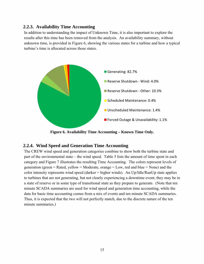
2.2.3. Availability Time Accounting In addition to understanding the impact of Unknown Time, it is also important to explore the results after this time has been removed from the analysis. An availability summary, without unknown time, is provided in Figure 6, showing the various states for a turbine and how a typical turbine’s time is allocated across those states.

Figure 6. Availability Time Accounting – Known Time Only.

2.2.4. Wind Speed and Generation Time Accounting The CREW wind speed and generation categories combine to show both the turbine state and part of the environmental state – the wind speed. Table 5 lists the amount of time spent in each category and Figure 7 illustrates the resulting Time Accounting. The colors represent levels of generation (green = Rated, yellow = Moderate, orange = Low, red and blue = None) and the color intensity represents wind speed (darker = higher winds). An Up/Idle/RunUp state applies to turbines that are not generating, but not clearly experiencing a downtime event; they may be in a state of reserve or in some type of transitional state as they prepare to generate. (Note that ten minute SCADA summaries are used for wind speed and generation time accounting, while the data for basic time accounting comes from a mix of events and ten minute SCADA summaries. Thus, it is expected that the two will not perfectly match, due to the discrete nature of the ten minute summaries.)

16

Table 5: Time Accounting, Wind Speed and Generation, Known Time Only.

Figure 7. Wind Speed and Generation Time Accounting – Known Time Only

17

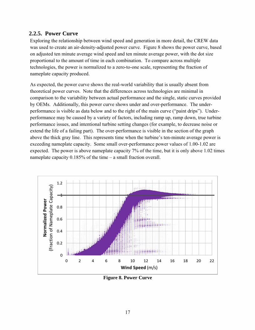
2.2.5. Power Curve Exploring the relationship between wind speed and generation in more detail, the CREW data was used to create an air-density-adjusted power curve. Figure 8 shows the power curve, based on adjusted ten minute average wind speed and ten minute average power, with the dot size proportional to the amount of time in each combination. To compare across multiple technologies, the power is normalized to a zero-to-one scale, representing the fraction of nameplate capacity produced.

As expected, the power curve shows the real-world variability that is usually absent from theoretical power curves. Note that the differences across technologies are minimal in comparison to the variability between actual performance and the single, static curves provided by OEMs. Additionally, this power curve shows under and over-performance. The under-performance is visible as data below and to the right of the main curve (“paint drips”). Under-performance may be caused by a variety of factors, including ramp up, ramp down, true turbine performance issues, and intentional turbine setting changes (for example, to decrease noise or extend the life of a failing part). The over-performance is visible in the section of the graph above the thick gray line. This represents time when the turbine’s ten-minute average power is exceeding nameplate capacity. Some small over-performance power values of 1.00-1.02 are expected. The power is above nameplate capacity 7% of the time, but it is only above 1.02 times nameplate capacity 0.185% of the time – a small fraction overall.

Figure 8. Power Curve

18

2.2.6. Wind Turbine Unavailability Contributors Recall that events currently come only from SCADA, and not yet from work orders or technician’s logs. Thus, the associated system and component are based on the indicated symptom, not necessarily the root cause. For example, a blade replacement is not captured by the SCADA as a blade replacement; instead, it is captured as general Unscheduled Maintenance and thus would be assigned to the “Wind Turbine (Other)” system.

2.2.6.1. Systems The system-level contributors to unavailability (downtime events only) are illustrated in Figure 9, ordered from greatest impact on unavailability to least. Compared to the 2011 Benchmark, less time falls into the “Wind Turbine (Other)” category, with it currently accounting for 63.7% of the downtime, compared to 71.7% in the 2011 Benchmark.

Figure 9. Unavailability Contributors, Top 10 Systems.

Unavailability is driven by two basic aspects of reliability – the frequency of downtime events (how often) and the duration of downtime events (how long). The systems in Figure 10 are ordered by their overall contribution to unavailability, but have their event frequency and event duration broken out. Event frequency is measured by the Annual Number of Events per Year per Turbine, which is the expected number of events per turbine per calendar year. Event duration is measured by Mean Downtime per Event, which is the average duration of a single event, in hours. Note that the generic system “Wind Turbine (Other)” dominates both frequency and downtime, due to a large number of SCADA events that do not have adequate detail to be assigned a more specific system. The Rotor/Blades and Generator systems have the most frequent downtime events, aside from “Wind Turbine (Other).” Compared to the 2011 Benchmark, there is much less variability in mean downtime across the systems.

19

Figure 10. Unavailability Contributors, System Event Frequency and Downtime.

Combining both the wind turbine system and the type of downtime event, Table 6 provides the Mean Time Between Events (MTBE) and Average Downtime (DT) for each combination of system and downtime event type (Forced, Scheduled Maintenance, and Unscheduled Maintenance). If no events are attributed to a given combination, the information is left blank.

Table 6. Wind Plant Reliability Model, System Detail.

20

As an example of how to use Table 6, one can calculate the frequency for Wind Turbine (Other) Maintenance, both Scheduled and Unscheduled. This corresponds to events where a technician has put the turbine into a maintenance or repair mode. The combined event rate is 0.00448 events per operating hour (= 1/429 + 1/465), or 223 operating hours per event, on average. In other words, a typical turbine generates for 9.3 days between technician lock-out events. Using a Utilization of 82.7%, a technician is visiting each turbine, on average, every 11.2 days, or 1.6 weeks. Presumably, technicians also visit the turbines at other times, too, so this provides an initial upper bound on the average time between visits.

2.2.6.2. Components The top ten component contributors to unavailability (downtime events only) are illustrated in Figure 11. Recall that these are component + event types that are attributable to a SCADA event. Note that “Wind Turbine---Unscheduled Maintenance” and “Wind Turbine---Scheduled Maintenance” are the two most common types listed, making up 60.7% of unavailability. This means that the majority of downtime occurs when the turbine itself is the most specific component that can be identified as the symptom or cause based on SCADA data.

Figure 11. Unavailability Contributors, Top 10 Component + Event Type contributors.

21

3.0 Observations

Event Frequency and Offshore Implications From the CREW reliability database, we found that an average turbine will actively generate power for 1.5 days between downtime events, with additional breaks for reserve events. The average downtime event lasts 1.6 hours. Focusing on just events when a technician has placed the turbine in maintenance or repair mode, there is a technician at the average turbine every 1.6 weeks. It remains to be seen whether this performance translates directly to offshore turbines, but the potential operations cost implications are staggering.

SCADA Symptoms versus Work Order Root Cause Excluding the “Wind Turbine (Other)” category, the top three system-level contributors to Turbine Unavailability were Rotor/Blades, Electric Generator, and Controls. The gearbox is notably absent from the top five systems. This may be due to a lack of insight into major maintenance, as SCADA data alone makes it very difficult to obtain detail about such repairs. To understand a complete reliability picture, it is critical to capture data from high quality electronic work orders and computerize maintenance management systems (CMMS), to enable root cause insight at the component level. A major part of the CREW team’s focus for 2012 and 2013 is providing the wind industry with information and tools to increase and improve the use of electronic work orders.

Improvements in Known Time A complete reliability picture requires insight into Unknown Time. Great strides have been made in improving the amount of Known Time, from less than 63% for the 2011 Benchmark, to over 70% cumulatively and some recent months above 80%. IT communications and SCADA issues are key contributors, and more work is still needed in prevention or early detection of these issues. The CREW team, SPS, and the partner plants are committed to continuous improvement in this area and are implementing new checks and alert systems.

22

Appendix A: Methodology and Calculations

Recent Data and Analysis Changes

Since the 2011 Benchmark report, there have been a few changes to the input data and/or analysis processes used. Those changes are summarized here.

Reclassified Reserve Events: With continued learning about OEM fault codes and procedures for ramp up and ramp down, many of the reserve events the CREW team previously categorized as “Reserve Shutdown – Wind” have been re-categorized as “Reserve Shutdown – Other.”

o If metric definitions are ambiguous, care has been taken to label or footnote output with whether it includes just downtime events or both downtime and reserve events.

Modified Definition of Operational Availability: After updating the reserve event classification, a large number of very short “Reserve Shutdown – Other” events were created. To appropriately model the impact of downtime events, the definition of Operational Availability was updated to consider all reserve events as “Available” (before only “Reserve Shutdown – Wind” events were considered “Available”).

o The classification of Reserve Events is a work in progress, and will continue to evolve as the breadth of the dataset grows and the team develops new approaches.

o Because the 2011 Reserve Shutdown – Other value was rounded to 0.0%, this change had no impact on the Operational Availability or Utilization metrics reported.

Data Quality and Completeness

Unknown time is treated as neither up-time nor downtime. The CREW team feels strongly that making further assumptions about this time can produce misleading results, and thus the time is reported and then treated as if it never existed. For example, in a 168 hour week, if 20 hours of data were missing, then the analysis is performed as if the turbines were monitored for 148 hours.

There are two types of data that result in Unknown Time for CREW calculations. The first is data that is simply missing. The second is data that is recorded, but is known to be bad. The most common cause is an overloaded server at the wind plant, which slows down or stops data updates to accommodate its load. Thus, the “new” data value is recorded as exactly what it was the moment before. When this happens for an entire 10 minute period, CREW considers the data to be “static” and therefore bad. When data is known to be bad for an entire ten minute period, the ten minute data is removed from the analysis. Additionally, each event corresponds to a number of ten minute periods; when more than half of these periods are bad, the event is removed from the analysis.

23

CREW Reliability Model

Individual Plant Models

The CREW team creates individual plant reliability models, by summarizing the ORAPWind® downtime events using the EBS components and general event types. The event downtime and the event frequency are modeled for each component + event type. For downtime events, Sandia’s Pro-Opta reliability analysis tool suite is used to create a fault-tree-based reliability model from the ORAPWind® downtime events. Pro-Opta summarizes the individual downtime events into a fault-tree model of a single, representative turbine. Then, it uses its algorithms and a simulation to create a downtime distribution and an event frequency distribution for each component + event type. It is the means of these distributions that the CREW team currently uses as input for the Benchmark and associated reporting, in the form of an average event frequency and mean downtime.

Due to their substantially larger volume of events, reserve events are processed separately from downtime events. A straight calculation, based on the total operating time and the total number of events for each component + event type, is used to calculate the event frequency for reserve events. As shown in Equation 1, this value can be calculated for each component + event type, for a single, representative turbine at the plant. Similarly, Equation 2 shows how the mean downtime can be found using the sum of event durations and the total number of events.

Equation 1. Event Frequency, Plant Model, Reserve Events.

,

∑ ,

∑

Equation 2. Mean Downtime, Plant Model, Reserve Events.

, . ∑ . ,

∑ .

Aggregation into CREW Reliability Model

Individual plant models, consisting of an event frequency and mean downtime for each component + event type, are aggregated into the CREW Reliability Model. It is important that there is sufficient data, both breadth and duration, to aggregate across plants without violating anonymity. At this point, downtime events and reserve events are both included and treated the same. The aggregation takes a weighted average, across plants, of the event frequency and

24

downtime values for each component + event type. The weight used is the number of turbine-days of known time for that plant. Compared to a simple average, this weighting scheme gives more influence to plants that have a large number of turbines, a longer data history, or both.

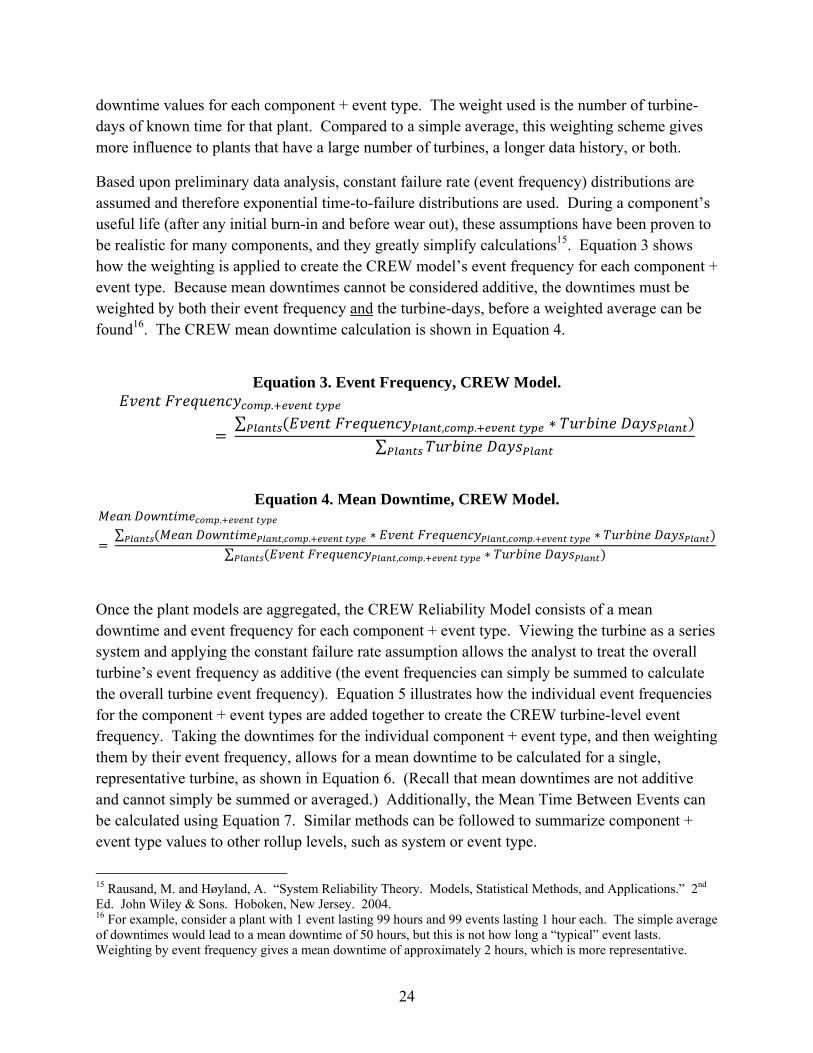
Based upon preliminary data analysis, constant failure rate (event frequency) distributions are assumed and therefore exponential time-to-failure distributions are used. During a component’s useful life (after any initial burn-in and before wear out), these assumptions have been proven to be realistic for many components, and they greatly simplify calculations15. Equation 3 shows how the weighting is applied to create the CREW model’s event frequency for each component + event type. Because mean downtimes cannot be considered additive, the downtimes must be weighted by both their event frequency and the turbine-days, before a weighted average can be found16. The CREW mean downtime calculation is shown in Equation 4.

Equation 3. Event Frequency, CREW Model.

.

∑ , . ∗

∑

Equation 4. Mean Downtime, CREW Model.

.

∑ , . ∗ , . ∗

∑ , . ∗

Once the plant models are aggregated, the CREW Reliability Model consists of a mean downtime and event frequency for each component + event type. Viewing the turbine as a series system and applying the constant failure rate assumption allows the analyst to treat the overall turbine’s event frequency as additive (the event frequencies can simply be summed to calculate the overall turbine event frequency). Equation 5 illustrates how the individual event frequencies for the component + event types are added together to create the CREW turbine-level event frequency. Taking the downtimes for the individual component + event type, and then weighting them by their event frequency, allows for a mean downtime to be calculated for a single, representative turbine, as shown in Equation 6. (Recall that mean downtimes are not additive and cannot simply be summed or averaged.) Additionally, the Mean Time Between Events can be calculated using Equation 7. Similar methods can be followed to summarize component + event type values to other rollup levels, such as system or event type.

15 Rausand, M. and Høyland, A. “System Reliability Theory. Models, Statistical Methods, and Applications.” 2nd Ed. John Wiley & Sons. Hoboken, New Jersey. 2004. 16 For example, consider a plant with 1 event lasting 99 hours and 99 events lasting 1 hour each. The simple average of downtimes would lead to a mean downtime of 50 hours, but this is not how long a “typical” event lasts. Weighting by event frequency gives a mean downtime of approximately 2 hours, which is more representative.

25

Equation 5. Single Turbine, Overall Event Frequency.

. .

Equation 6. Single Turbine, Overall Mean Downtime.

∑ . ∗ . .

∑ . .

Equation 7. Single Turbine, Overall Mean Time Between Events.

1

Basic Time Accounting

In addition to the plant reliability models, the CREW team also calculates time accounting results. The categories are: Generating, Reserve Shutdown – Wind, Reserve Shutdown – Other, Scheduled Maintenance, Unscheduled Maintenance, Forced Outage and Unavailability, and Unknown Time. The total time spent in each event type category is found by summing the “downtimes” (durations) for the appropriate type of downtime event or reserve event. The total amount of Generating time is calculated by summing all of the ten minute periods where the mode of the turbine state indicates it is connected to the grid and making power. This simple method of summing durations naturally provides greater impact from plants that have a large number of turbines, a longer data history, or both. Lastly, the Unknown Time can be calculated by finding the total number of hours in the data timeframe, and subtracting all the time in the other categories. If all data was fully and correctly captured, there would be no leftover.

Operational Availability is defined as the percent of known time that the turbines are not experiencing any downtime events. This is equivalent to calculating the percent of known time that the turbines are either generating or in reserve, as shown in Equation 8. Similarly, Utilization (also known as Generating Factor) is defined as the percent of known time that the turbines are generating, as shown in Equation 9. The various time categories can be used to calculate other availability metrics for comparison to one’s own key performance indicators (KPIs).

Equation 8. Operational Availability.

26

Equation 9. Utilization (i.e., Generating Factor).

Wind Speed and Generation Time Accounting

The CREW Benchmark also includes a section on time accounting that focuses on Wind Speed and Generation, which are defined by the categories in Table 7 and Table 8.

Table 7. Wind Speed Categories. Wind Speed Category Definition None or Below Cut In ≤ Cut In m/s Moderate Cut In – 11 m/s Rated 11 – Cut Out m/s Above Cut Out > Cut Out m/s Unknown Missing, Blank, or > 100 m/s

Table 8. Power Generation Categories.

Generation Definition None ≤ 0% of Nameplate Capacity Low 0 – 10% of Nameplate Capacity Moderate 10 – 90% of Nameplate Capacity Rated 90 – 100% of Nameplate Capacity Over-Rated 100 – 200% of Nameplate Capacity Unknown Missing, Blank, or > 200% Nameplate

When Generation is None, a distinction is drawn between turbines in a “Down” state versus turbines in an “Up/Transition” state. A Down state applies to turbines that are experiencing a downtime event. An Up/Transition state applies to turbines that are not generating and not experiencing a downtime event; they should be in a state of reserve. The metrics for Wind Speed and Generation Time Accounting are created by first taking each combination of wind speed category, generation category, and (if applicable) Down or Up status. This categorization is done for each turbine, for each ten minute period. The ten minute average power, average wind speed, and most common operating state (statistical mode) are used for the assignment. Then, the total amount of time (in ten minute increments) the turbines spend in each combination category is summed to create the values that are reported.

27

Power Curve

To create power curves, the CREW team follows the guidance of the International Electrotechnical Commission (IEC) standard 61400-12, “Wind turbine generator systems – Part 12: Wind turbine power performance testing”.17 To calculate the air-density-adjusted wind speed for a given ten minute period, the CREW team uses the following steps.

For each plant, for each ten minute period: 1. Calculate the average air temperature [K], by averaging all high resolution SCADA air

temperature observations from each met tower. If a site utilizes multiple met towers, then these values are averaged across met towers to create a plant value.

2. Calculate the average air pressure [Pa] by averaging all the high resolution SCADA air pressure observations from the met tower. If a site utilizes multiple met towers, then these values are averaged across met towers to create a plant value.

3. Use Equation 10 to calculate the derived air density [kg/m3] using the average air temperature, average air pressure, and the gas constant R [measured in J/(kg*K)].

Equation 10. Derived Air Density. / ∗

For each turbine, for each ten minute period:

4. Calculate the average wind speed [m/s] by averaging the high resolution SCADA wind speed observations from the turbine.18

5. Use Equation 11 to calculate the adjusted average wind speed, using a reference air density [1.225 kg/m3], the derived air density based on the met tower data, and the turbine’s average wind speed.

Equation 11. Adjusted Wind Speed.

∗

/

6. Round the adjusted wind speed down to the nearest 0.25 m/s. 7. Use Equation 12 to calculate the normalized power, using the average power and the

nameplate capacity. Then, round this value down to the nearest 0.01.

17 International Electrotechnical Commission. “Wind turbine generator systems – Part 12: Wind turbine power performance testing.” IEC 61400-12. Geneva, Switzerland. 1998. 18 The wind speeds recorded at the turbine and at the met tower frequently differ by a few meters per second. Having explored power curves based on the met tower wind speed and the turbine’s wind speed, the CREW team has found the wind turbine’s recorded speed better aligns with power output, and therefore is a better signal to use.

28

Equation 12. Adjusted Wind Speed.

Lastly: 8. For each unique combination of rounded adjusted wind speed and rounded normalized

power, count the number of ten minute periods observed with these values.

In the power curve graph, the point size plotted is proportional to the count of rounded observations. Only positive values for rounded adjusted wind speed and rounded normalized power are used in the graph.

Other Calculations

Many other calculations are possible from the information calculated above and from other data in the CREW database. For example, Annual Average Event Rate can be calculated, which is simply another way of looking at event frequency, . The Annual Average Event Rate is the expected number of downtime events per turbine per calendar year, and it can be calculated using Equation 13. There are approximately 8760 hours per calendar year, thus multiplying Utilization by 8760 results in the number of generating hours per year. Multiplying the number of generating hours per year by the number of events per generating hour (also known as the Event Frequency) results in the number of events per year.

Equation 13. Annual Average Event Rate. ∗ 8760 ∗

The Capacity Factor calculation is different from many of the others defined so far, as it is not based upon categorizing time. The Capacity Factor is defined as the percent of nameplate capacity that the turbines generated, over some data timeframe of interest. Another way of calculating Capacity Factor is averaging the instantaneous power, over some data timeframe of interest, and then dividing this by the nameplate instantaneous power. Equation 14 uses this second approach. Note that it only covers known time (i.e., time when the power output is actually known).

Equation 14. Capacity Factor.

29

Equipment Breakdown Structure

CREW uses the SPS EBS, which has a four-level hierarchy, with levels for major system, system, component group, and component. The full EBS is proprietary to SPS, though Figure 12 shows an excerpt. For example, the component “Up-Wind Carrier Bearing,” has “Wind Turbine” as its major system, “Gearbox” as its system, and “Bearings” as its component group.

Figure 12. Equipment Breakdown Structure Excerpt.

Other Assumptions

A variety of assumptions are made during data preparation, analysis, and reporting. Assumptions not already captured elsewhere in this report are listed below.

If a plant does not experience any instances of an event with a given component + event type, then that plant is not included in the calculations for that component + event type. This may slightly increase the event frequency for events that could occur at a plant, but have not yet.

Back-to-back events are counted separately. For example, consider a turbine that is down for a period of time, very briefly returns to service, immediately goes down again, and then eventually returns to service. This situation would result in two events, both of which are included in the analysis and contribute to the event frequency and duration.

Events with no duration are given 0.0001 hours (0.36 seconds) of downtime. These events contribute to increased event frequency and decreased mean downtimes. Typically these events occur because the SCADA can process data on the order of milliseconds, and the ORAPWind® system captures data on the order of seconds. Thus, an event that lasts for milliseconds can appear as if it began and ended at exactly the same time.

30

Appendix B: Nomenclature Annual Average Event Rate: the expected number of events per calendar year

Availability: see “Operational Availability”

AWEA: American Wind Energy Association

Capacity Factor: the percent of total nameplate capacity that was actually generated, factoring in only time when the generation is known

CMMS: Computerized Maintenance Management System

Component: lowest level of the Equipment Breakdown Structure

CREW: Continuous Reliability Enhancement for Wind

Cut In (wind speed): theoretically, the minimum wind speed at which a turbine can generate power

Cut Out (wind speed): theoretically, the maximum wind speed at which a turbine can generate power

Data Timeframe: time period over which data was collected and analyzed

DOE: Department of Energy

Downtime Event: SCADA fault state that stops the turbine and takes it out of service (both automatic & manual stops), including technician work when the turbine is stopped

DT: Average Downtime

EBS: (Equipment Breakdown Structure); logical hierarchy of components for a wind turbine

EERE: Energy Efficiency and Renewable Energy

Event: SCADA state that either stops the turbine, takes it out of service, or indicates that it is not generating; an event is either a downtime event or a reserve event

Event Frequency: the expected number of events per generating hour; unless otherwise specified, the CREW values only include downtime events

Forced (Outage or Unavailability): unplanned downtime event indicating a fault or failure (e.g., automatic trip; manual stop by operator)

Generating Factor: see “Utilization”

IEC: International Electrotechnical Commission

IT: Information Technology

Known Time: time when the SCADA data has been fully transferred into CREW and is also usable for analysis

KPI: Key Performance Indicator

Mean Downtime: the average duration of an event, in hours; unless otherwise specified, the CREW values only include downtime events

Met Tower: Meteorological Tower

MTBE: (Mean Time Between Events); average number of generating hours between events; unless otherwise specified, the CREW values only include downtime events

MW: Megawatt

31

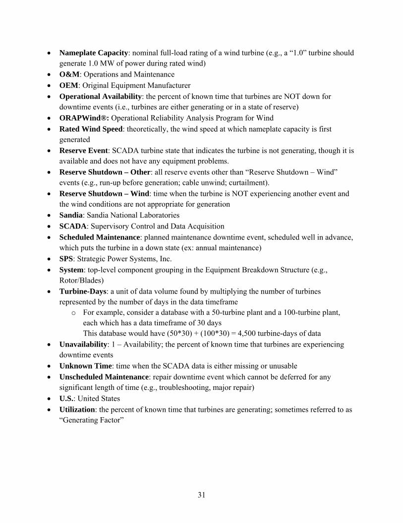
Nameplate Capacity: nominal full-load rating of a wind turbine (e.g., a “1.0” turbine should generate 1.0 MW of power during rated wind)

O&M: Operations and Maintenance

OEM: Original Equipment Manufacturer

Operational Availability: the percent of known time that turbines are NOT down for downtime events (i.e., turbines are either generating or in a state of reserve)

ORAPWind®: Operational Reliability Analysis Program for Wind

Rated Wind Speed: theoretically, the wind speed at which nameplate capacity is first generated

Reserve Event: SCADA turbine state that indicates the turbine is not generating, though it is available and does not have any equipment problems.

Reserve Shutdown – Other: all reserve events other than “Reserve Shutdown – Wind” events (e.g., run-up before generation; cable unwind; curtailment).

Reserve Shutdown – Wind: time when the turbine is NOT experiencing another event and the wind conditions are not appropriate for generation

Sandia: Sandia National Laboratories

SCADA: Supervisory Control and Data Acquisition

Scheduled Maintenance: planned maintenance downtime event, scheduled well in advance, which puts the turbine in a down state (ex: annual maintenance)

SPS: Strategic Power Systems, Inc.

System: top-level component grouping in the Equipment Breakdown Structure (e.g., Rotor/Blades)

Turbine-Days: a unit of data volume found by multiplying the number of turbines represented by the number of days in the data timeframe

o For example, consider a database with a 50-turbine plant and a 100-turbine plant, each which has a data timeframe of 30 days This database would have (50*30) + (100*30) = 4,500 turbine-days of data

Unavailability: 1 – Availability; the percent of known time that turbines are experiencing downtime events

Unknown Time: time when the SCADA data is either missing or unusable

Unscheduled Maintenance: repair downtime event which cannot be deferred for any significant length of time (e.g., troubleshooting, major repair)

U.S.: United States

Utilization: the percent of known time that turbines are generating; sometimes referred to as “Generating Factor”

32

DISTRIBUTION:

4 U.S. Department of Energy Wind and Water Power Program Attn: Michael Derby (Electronic Copy) Cash Fitzpatrick (Electronic Copy) Mark Higgins (Electronic Copy) Jose Zayas (Electronic Copy)

Washington, DC 20585 1 MS 1104 J. Torres, 06120 (Electronic Copy) 1 MS 1124 C. Bond, 06121 (Electronic Copy) 1 MS 1124 D. Minster, 06121 (Electronic Copy) 1 MS 1124 A. Ogilvie, 06121 (Electronic Copy) 1 MS 1124 D. Laird, 06122 (Electronic Copy) 1 MS 9406 V. Peters, 06121 (Electronic Copy) 1 MS 0899 Technical Library, 9536 (Electronic Copy)