3

SAND97-1652 DistributionUnlimited Release Category UC-122

Printed November 1997

Finite Element Analysis of Sucker Rod Couplings with Guidelines for Improving Fatigue Life

Edward L. HoffmanEngineering and Structural Mechanics Division

Sandia National LaboratoriesAlbuquerque, New Mexico 87185

Abstract

The response of a variety of sucker rod couplings to an applied axial load was simulated usingaxisymmetric finite element models. The calculations investigated three sucker rod sizes andvarious combinations of the slimhole, Spiralock, and Flexbar modifications to the coupling. Inaddition, the effect of various make-ups (assembly tightness) on the performance of couplingwas investigated. The make-up process, based on measured circumferential displacement ofthe coupling from a hand-tight position, was simulated by including a section of an axiallyexpanding material in the box section which, when heated, produced the desired mechanicalinterference which would result from making-up the coupling. An axial load was applied tothe sucker rod ranging from -5 ksi to 40 ksi, encompassing three load cycles identified on amodified Goodman diagram as acceptable for indefinite service life of the sucker rods. Thesimulations of the various coupling geometries and make-ups were evaluated with respect tohow well they accomplish the two primary objectives of preloading threaded couplings: (1) tolock the threaded coupling together so that it will not loosen and eventually uncouple, and (2)to improve the fatigue resistance of the threaded connection by reducing the stress amplitudein the coupling when subjected to cyclic loading. A coupling will remain locked as long as themating surfaces of the pin and box sections remain in compression, resisting rotational motionor loosening. The fatigue evaluation was accomplished in two parts: nominally and locally. Inthe nominal evaluation, a set of equations based on the gross dimensions of the coupling werederived which describe how a load applied to a sucker rod is distributed throughout apreloaded coupling. The local fatigue evaluation characterized the fatigue performance of thevarious couplings using the local stresses predicted in the finite element simulations and astress equivalencing criterion for multiaxial stress states. This criterion is based on Sines’equivalent stress theory which states that the permissible effective alternating stress is a linearfunction of the mean hydrostatic stress. Perhaps the most significant finding in this study wasthe characterization of the coupling parameters which affect these two stress measures. Themean hydrostatic stress, which determines the permissible effective alternating stress, is afunction of the coupling make-up. Whereas, the alternating effective stress is a function of therelative stiffnesses of the pin and box sections of the coupling and, as long as the couplingdoes not separate, is unaffected by the amount of circumferential displacement applied duringmake-up. The results of this study suggest approaches for improving the fatigue resistance ofsucker rod couplings.

4

5

Contents

Figures. . . . . . . . . . . . . . . . . . . . . . . . . . . . . . . . . . . . . . . . . . . . . . . . . . . . . . . . . . . . . . . . . . . . 6

Tables . . . . . . . . . . . . . . . . . . . . . . . . . . . . . . . . . . . . . . . . . . . . . . . . . . . . . . . . . . . . . . . . . . . . 8

1 Introduction. . . . . . . . . . . . . . . . . . . . . . . . . . . . . . . . . . . . . . . . . . . . . . . . . . . . . . . . . . . . . 9

2 Analysis Model . . . . . . . . . . . . . . . . . . . . . . . . . . . . . . . . . . . . . . . . . . . . . . . . . . . . . . . . . 12

2.1 Finite Element Model of the Coupling Geometry . . . . . . . . . . . . . . . . . . . . . . . . . . 12

2.2 Preload of Sucker Rod Couplings . . . . . . . . . . . . . . . . . . . . . . . . . . . . . . . . . . . . . . 13

2.3 Materials and Load History . . . . . . . . . . . . . . . . . . . . . . . . . . . . . . . . . . . . . . . . . . . 15

2.4 Summary of Analysis Cases. . . . . . . . . . . . . . . . . . . . . . . . . . . . . . . . . . . . . . . . . . . 17

3 Analysis Results . . . . . . . . . . . . . . . . . . . . . . . . . . . . . . . . . . . . . . . . . . . . . . . . . . . . . . . . 18

3.1 Yielding in the Sucker Rod Coupling . . . . . . . . . . . . . . . . . . . . . . . . . . . . . . . . . . . 18

3.2 Load Distribution in Threaded Coupling During Load Cycling . . . . . . . . . . . . . . . 21

3.3 Estimating Fatigue Life of Sucker Rod Couplings. . . . . . . . . . . . . . . . . . . . . . . . . . 31

3.3.1 Considerations in Life Prediction . . . . . . . . . . . . . . . . . . . . . . . . . . . . . . . . . . 32

3.3.2 Fatigue Damage Criterion for Multiaxial Stress. . . . . . . . . . . . . . . . . . . . . . . 34

3.3.3 Identification of Critical Fatigue Locations . . . . . . . . . . . . . . . . . . . . . . . . . . 38

3.3.4 Equivalent Stress at Critical Locations. . . . . . . . . . . . . . . . . . . . . . . . . . . . . . 38

Root of First Engaged Pin Thread . . . . . . . . . . . . . . . . . . . . . . . . . . . . . . . 44

Pin Neck . . . . . . . . . . . . . . . . . . . . . . . . . . . . . . . . . . . . . . . . . . . . . . . . . . 48

Root of Last Engaged Box Thread . . . . . . . . . . . . . . . . . . . . . . . . . . . . . . 53

3.3.5 Effect of Make-up on Service Life . . . . . . . . . . . . . . . . . . . . . . . . . . . . . . . . . 60

4 Conclusions and Recommendations . . . . . . . . . . . . . . . . . . . . . . . . . . . . . . . . . . . . . . . . . 63

References. . . . . . . . . . . . . . . . . . . . . . . . . . . . . . . . . . . . . . . . . . . . . . . . . . . . . . . . . . . . . . . . 65

Distribution . . . . . . . . . . . . . . . . . . . . . . . . . . . . . . . . . . . . . . . . . . . . . . . . . . . . . . . . . . . . . . . 66

6

Figures

Figure 1. Illustration of sucker rod pump. 9

Figure 2. Threaded pin and shoulder at each end of the sucker rod. 10

Figure 3. Modified Goodman diagram for allowable stress and range of stress for sucker rods in non-corrosive service. 11

Figure 4. Detailed illustrations of the 7/8-inch coupling, with dimensions of the coupling and the threads. 12

Figure 5. Axisymmetric finite element model of 7/8 inch sucker rod coupling, showing the pin and box sections. 13

Figure 6. Existing sucker rod coupling designs and proposed design modifications under investigation. 14

Figure 7. Modified Goodman diagram for API Grade C carbon steel, identifying load cycles and extreme loads selected for analysis. 16

Figure 8. Von Mises stress distribution (ksi) in the 7/8-inch API standard coupling (Analysis 1) at preload, maximum compression, and maximum tensile loads. 19

Figure 9. Von Mises stress distribution (ksi) in the 7/8-inch Spiralock coupling (Analysis 12) at preload, maximum compression, and maximum tensile loads. 20

Figure 10. Illustration of sucker rod coupling. 21

Figure 11. Pin load and coupling force as a function of axial load for the 3/4, 7/8, and 1-inch coupling sizes (S6, S7, and S8, respectively). 26

Figure 12. Pin load and coupling force as a function of axial load for the 7/8-inch standard API coupling size (S7) with make-ups of 0.0, 1.0, and 1.5. 27

Figure 13. Pin load and coupling force as a function of axial load for various combinations of the Flexbar (FB), Spiralock (SL), and slimhole (SH) geometry modifications to the base geometry (S7). 29

Figure 14. Pin load and coupling force as a function of axial load for the base geometry (S7) with Spiralock threads (SL) and make-ups of 0.0, 1.0,1.5, 2.0, 2.5, and 3.0. 30

Figure 15. Schematic S-N curves for steel at various stress ratios. 34

Figure 16. Maximum principal stress directions in the 7/8-inch API standard coupling at minimum (-5 ksi) and maximum (40 ksi) loads. 35

Figure 17. Distribution of the fatigue safety factor with respect to indefinite service life for the 7/8-inch API standard coupling subjected to the three load cycles. 39

Figure 18. Distribution of the effective alternating stress in the 7/8-inch API standard coupling subjected to the three load cycles. 40

Figure 19. Distribution of the hydrostatic mean stress in the 7/8-inch API standard coupling subjected to the three load cycles. 41

7

Figure 20. Difference between the effective alternating stress and the alternating effective stress in the 7/8-inch API standard coupling subjected to the three load cycles. 42

Figure 21. Von Mises and hydrostatic stress at the root of the first engaged pin thread as a function of applied axial load for various coupling sizes. 45

Figure 22. Von Mises and hydrostatic stress at the root of the first engaged pin thread as a function of applied axial load for various make-ups of the 7/8-inch API coupling. 46

Figure 23. Von Mises and hydrostatic stress at the root of the first engaged pin thread as a function of applied axial load for various combinations of the Flexbar (FB), slimhole (SH), and Spiralock (SL) modifications to the base coupling (S7). 47

Figure 24. Von Mises and hydrostatic stress at the root of the first engaged pin thread as a function of applied axial load for the Spiralock coupling with make-ups of 0.0, 1.0, 1.5, 2.0, 2.5, and 3.0. 49

Figure 25. Von Mises and hydrostatic stress at the pin neck as a function of applied axial load for various coupling sizes. 50

Figure 26. Von Mises and hydrostatic stress at the pin neck as a function of applied axial load for various make-ups of the 7/8-inch API coupling. 51

Figure 27. Von Mises and hydrostatic stress at the pin neck as a function of applied axial load for various combinations of the Flexbar (FB), slimhole (SH), and Spiralock (SL) modifications to the base coupling (S7). 52

Figure 28. Von Mises and hydrostatic stress at the pin neck as a function of applied axial load for the Spiralock coupling with make-ups of 0.0, 1.0, 1.5, 2.0, 2.5, and 3.0. 54

Figure 29. Von Mises and hydrostatic stress at the root of the last engaged box thread as a function of applied axial load for various coupling sizes. 55

Figure 30. Von Mises and hydrostatic stress at the root of the last engaged box thread as a function of applied axial load for various make-ups of the 7/8-inch API coupling. 57

Figure 31. Von Mises and hydrostatic stress at the root of the last engaged box thread as a function of applied axial load for various combinations of the Flexbar (FB), slimhole (SH), and Spiralock (SL) modifications to the base coupling (S7). 58

Figure 32. Von Mises and hydrostatic stress at the root of the last engaged box thread as a function of applied axial load for the Spiralock coupling with make-ups of 0.0, 1.0, 1.5, 2.0, 2.5, and 3.0. 59

Figure 33. Fatigue safety factor distribution in the 7/8-inch Spiralock coupling (with make-ups of 1.0, 1.5, and 2.0) subjected to the full axial load range (-5 ksi to 40 ksi). 61

8

Tables

Table 1. API Sucker Rod Joint Make-up Recommendations . . . . . . . . . . . . . . . . . . . . . . . 15

Table 2. Summary of Analysis Cases . . . . . . . . . . . . . . . . . . . . . . . . . . . . . . . . . . . . . . . . . 17

Table 3. Pin and Box Cross-Sectional Areas and Load Partitioning Factors for Various Cou-pling Geometries. . . . . . . . . . . . . . . . . . . . . . . . . . . . . . . . . . . . . . . . . . . . . . . . . . . . . . . . . . . 24

Table 4. Summary of Coupling Performance for Various Analysis Cases . . . . . . . . . . . . . 31

9

1 Introduction

Oil and gas production in the US has reached a point where significant effort is required toforestall declining production and stop the abandonment of significant unproduced resources.New technology developments are needed. However, because lifting costs are high relative tooil prices, the petroleum industry is downsizing and investing less effort in the development ofnew technology. The goal of Sandia National Laboratories’ Applied Production Technology(APT) project is to extend the life of marginally economic wells by reducing the negativeimpacts of persistent production problems. The approach is to use “Sandia Technology” torapidly diagnose industry-defined production problems and then propose or develop improvedtechnology utilizing the capabilities of industry. One task of the APT project is theinvestigation of sucker rod and sinkerbar failures. Sucker rods and sinker bars are the primarycomponents of rod pumping systems, the most common artificial lift technology utilized indomestic oil production. Thus, high sucker rod failure rates have a large economic impact onthe domestic oil industry and threaten the domestic oil reserves with high abandonment rates.If the level of technology and understanding of the rod pumping system can be increased,there will be significant benefit to both the domestic industry and domestic energy security.

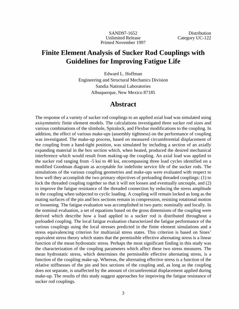
A sucker rod pump, illustrated inFigure 1, brings underground oil tothe earth's surface. The primary drivemotor turns a flywheel with a crankarm. Attached to the crank arm is aPitman Arm which links the crank tothe

walking beam

. The walking beanis a lever arm which pivots at itsmidsection. At the other end of thewalking beam is the

horsehead

. Ahanger cable hangs off the horseheadand is clamped to the rod string. Thismechanism converts the rotarymotion of the drive motor to atranslational pumping motion. Twovalves are used to maintain thedirection of flow. A traveling valve,often just a ball in a cage, is attachedto a plunger at the end of the rodstring. At the base of the well is astationary valve (another ball in acage) called a standing valve.

The rod string, capable of reachinglengths of over 10,000 ft, consists ofindividual sections of steel rods calledsucker rods. Sucker rods come inlengths ranging from 25 to 30 ft and Figure 1. Illustration of sucker rod pump.

Pitman Arm

Traveling Valve

Horse Head

Standing Valve

Flywheel & Crank Arm

10

nominal diameters ranging from 0.5 to 1.125 inches. Each rod contains a threaded pin at eachend as shown in Figure 2. Threaded couplings, known as

boxes

, are used to connect the suckerrods to produce the rod string. These pin and box coupling are tightened to a specifiedpreload, known as the joint

make-up

, so that it will not loosen during normal operation.

In addition to supporting the pumping forces, each sucker rod must be strong enough tosupport the weight of the rods below it. Hence, loads are greater on the sucker rods farther upthe rod string. The diameter of each sucker rod is specified by the well designer based on thestrength of the rod material and the loads it will be exposed to. As most rod strings are madeup of a single material, the resulting optimized rod string tapers down in diameter withdistance down the well. Because the rod string is extremely long relative to its diameter,elastic stability of this long slender column is of concern to pump designers. The rod stringmust translate the force to the pump in

both

stroke directions. Because the entire length of therod string will be in tension on the upward stroke, elastic stability of the rod string is not aproblem. Furthermore, if the weight of the rod string exceeds the required pumping force onthe downward stroke (as it typically does), then the upper sucker rods will also be in tensionon the downward stroke. The lower rods, on the other hand, will be in compression on thedownstroke, a condition which could result in downstroke compression buckling of the lowerrods. To keep the rod string straight and in tension throughout the pump cycle, a section oflarge diameter bar, known as a

sinker bar

, is placed just above the pump. The sinker bar,typically consisting of large-diameter sucker rods (such as 7/8 or 1-inch), replaces an equallength of sucker rods immediately above the pump. This large diameter section of the rodstring is both heavy enough to keep the sucker rods in tension and stiff enough to resistbuckling. The sinker bar may also increase pump plunger overtravel (on the downstroke)which increases fluid production.

Rod string failures are very expensive to repair since the entire string must be disassembledand removed to access the failed rod. The rod string must then be reassembled. Wells withlow production rates may not warrant the cost of repairing a failed rod. To maximize systemreliability, safety and simplify system design, nearly every aspect of sucker rod system design,manufacturing and assembly has been standardized by the American Petroleum Institute(API). Because sucker rods are exposed to cyclic stresses, they are at risk of fatigue failure.Fatigue is the process of cumulative damage caused by repeated fluctuating loads whosemagnitude is well below the material’s ultimate strength under monotonic loading. To ensurea long fatigue life of the sucker rods, the API uses the modified Goodman stress diagram

polished rod

Figure 2. Threaded pin and shoulder at each end of the sucker rod.

Df

Df = Pin Shoulder DiameterWs = Wrench Square Width

Ws

11

(shown in Figure 3) to determine the allowable range of stress for a sucker rod. Based on theultimate tensile strength of the material, the modified Goodman diagram defines a stressenvelope (shaded area) within which a structural component can operate such that it willprovide an infinite service life. Using this system, the well designer can determine theappropriate rod diameter based on a knowledge of the minimum load (on the downstroke) andthe maximum load (on the upstroke). The modified Goodman diagram provides thefundamental rating which can be used where corrosion is not a factor. Since all well fluids arecorrosive to some degree, the stress values determined from this diagram must be adjusted byan appropriate service factor based on the severity of the corrosion.

In spite of the thorough efforts of the API to ensure performance within the fatigue limits ofthe selected materials, sucker rod failures still occur. Pin failures comprise a large fraction ofall rod pumped system failures. Not much is known about the performance of sucker rodcouplings as they have not been extensively studied in the past. Because the coupling diameteris much larger than that of the rod, it has been assumed that the oversized coupling falls withinthe stress range specified by the Goodman diagram for the rod. This may not be true as thecoupling is a complex preloaded mechanism which will react differently to axial loads than asolid rod. This report documents finite element simulations of the sucker rod coupling whichwere performed to provide a better understanding of sucker rod couplings and attempt toexplain pin failures. All of the simulations were performed with JAC2D [1], a quasistaticfinite element analysis code developed at Sandia National Laboratories.

T

T T

T

1.75

0S min

= M

inimum

Stre

ss

SA = Allowable Stress

T4

Figure 3. Modified Goodman diagram for allowable stress and range of stress for sucker rods in non-corrosive service.

SA = (0.25T + 0.5625 Smin)SF∆SA = SA - Smin

Where:T = Minimum Tensile StrengthSF = Service FactorSA = Maximum Allowable Stress∆SA =Maximum Allowable Range of Stress

Minimum Stress

Str

ess

T2

T3

T3-

+

Sy

12

2 Analysis Model

2.1 Finite Element Model of the Coupling Geometry

Detailed illustrations of the 7/8-inch coupling, with dimensions of the coupling and threads,are shown in Figure 4. An axisymmetric finite element representation of the sucker rodcoupling is shown in Figure 5 with the axis of symmetry on the left side of the model.Although the threaded connection is a three-dimensional geometry, it can be adequatelyrepresented with an axisymmetric model since the thread pitch is small relative to the otherdimensions of the coupling. Because the lower boundary of the box section is modeled with asymmetry plane, the model represents the coupling of two rods. The pin is modeled up to theshoulder and does not include the narrower rod section. This simplification was made to avoidmodeling the asymmetric wrench flats which are located between the rod and the couplingshoulder. Since the applied loads are specified (from the Goodman plots) as stresses in therod, the resulting stress at the larger diameter coupling shoulder was required as input into themodel. This was accomplished by specifying a pressure multiplier equal to the ratio of the rodarea to the shoulder area.

Four existing sucker rod designs and five proposed design modifications were the subjects ofthis computational study. The various sucker rod pin designs and proposed pin modificationsare shown in Figure 6. The four existing sucker rod couplings studied here include thestandard couplings for 3/4, 7/8, and 1-inch sucker rods. In addition, a 7/8-inch slimhole

SHOULDER(intentional overlap to

achieve prestress)

PIN

BOX

DISTANT END OF PIN(pinned bc)

DISTANT END OF BOX

(pinned or load bc)

1.625" dia.

1.8125" dia.

1.040" dia.

1.205" dia.

1.625"

0.672"

2.125"1.79"

UNDERCUT REGION(length = 0.672")

ROOT OF FIRST BOX THREAD

FIRST ENGAGED THREAD

LAST ENGAGED THREAD

axis

of s

ymm

etry

(Exploded View)(Cross-sectional View)

SHOULDER

30 °

7/8" PIN

BOX

MAX. BOX MAJOR DIAM. (1.1880")

MIN. PIN MAJOR DIAM. (1.1732")

MAX. BOX PITCH DIAM. (1.1310")

MIN. PIN PITCH DIAM. (1.1150")

MAX. BOX MINOR DIAM. (1.101")

1/2 PIT

CH

= 0.05 "(10 T

HR

EA

DS

PE

R IN

CH

)

0.00416"

0.01083"

7/8" API Box and Pin Sucker Rod Connection

(Thread Detail)

Figure 4. Detailed illustrations of the 7/8-inch coupling, with dimensions of the coupling and the threads.

13

coupling, used in applications of low well bore clearance, is also studied. The five modifiedgeometries are variations of two basic modifications: the Flexbar pin, and Spiralock box. TheFlexbar pin uses the same coupling as the standard sucker rod coupling designs. However, thepin is slightly longer and incorporates a shoulder on which the coupling rests. The secondmodification consists of a proprietary thread design, called Spiralock threads, which are usedin the box section of the coupling. The pin retains the standard API threads in thisconfiguration.

2.2 Preload of Sucker Rod Couplings

The API sucker rod tables contain recommendations for the assembly or preloading of suckerrod couplings, also known as

make-up

. The recommendations are based on a circumferentialdisplacement, measured at the shoulder of the sucker rod, while tightening from a hand-tightposition. These recommendations are summarized in Table 1 for the 3/4, 7/8, and 1-inchdiameter sucker rods. The axial displacement of the pin (or interference at the shoulder) canbe calculated as:

Figure 5. Axisymmetric finite element model of 7/8 inch sucker rod coupling, showing the pin and box sections.

axially expanding material

axis

of s

ymm

etry

symmetry boundary condition

pressure boundarycondition

Pin Section

Box Section

14

Figure 6. Existing sucker rod coupling designs and proposed design modifications under investigation.

3/4” Sucker RodAPI Threads

7/8” Sucker RodAPI Threads

1” Sucker RodAPI Threads

7/8” Sucker RodAPI Threads

Slimhole Coupling

7/8” Sucker RodFlexbar Pin

7/8” Sucker RodFlexbar Pin

Slimhole Coupling

7/8” Sucker RodSpiralock Threads

7/8” Sucker RodSpiralock Threads

Flexbar Pin

7/8” Sucker RodSpiralock ThreadsSlimhole Coupling

(a) Existing Sucker Rod Coupling Designs

(b) Proposed Modifications to Sucker Rod Coupling Designs

15

(1)

where

P

is the thread pitch,

d

c

is the circumferential displacement, and

D

f

is the shoulderdiameter. All of the sucker rod sizes listed in Table 1 have a thread pitch of 0.1 inches.Simulating the preloading of the threaded coupling posed a particularly difficult problem. Theinterferences listed in Table 1 were large enough that the initial stress-free mesh required asignificant amount of mesh overlay at the pin-shoulder/box interface. The contact and solutionalgorithms of JAC2D had difficulty pushing back the overlapping meshes and converging ona solution. This was further complicated by the fact that in some cases the pin and boxsections exhibited a slight amount of yielding on preload, making joint preload a nonlinearevent. To circumvent these difficulties, a section of material was added to the box sectionwhich is identical to the box material except that it has an axial thermal expansion coefficient(see Figure 5). Preload was obtained by heating the model so that this section of materialexpanded, producing the required amount of displacement to preload the joint.

2.3 Materials and Load History

Since the API specifies allowable stress ranges for sucker rods based on the grade of steelused, the load history is coupled to the material selection. The API specifies many grades ofsteels for use in sucker rods and box couplings, depending on the particular application andload history. An API Grade C carbon steel was selected as the subject for this study. The APIGrade C specification includes any steel with a minimum yield strength of 60 ksi, and aminimum tensile strength of 90 ksi. Hence, these inelastic properties were used in the present

Table 1: API Sucker Rod Joint Make-up Recommendations

Rod Size (in)

Pin Shoulder OD (in)

Minimum Circumferential

Displacement (in)

Calculated axial displacement or interference (in)

3/4 1.500 7/32 4.64x10-3

7/8 1.625 9/32 5.51x10-3

1 2.000 12/32 5.97x10-3

Hand-tight joint Made-up joint

Scribed vertical Line

Measured circum-ferential displace-ment

di

Pdc

πD f----------=

16

study. The post yield behavior was modeled with a linear hardening modulus of 100 ksi. Inaddition, an elastic modulus of 29

×

10

6

psi and a Poisson’s ratio of 0.3 were used.

The fatigue limits of API Grade C sucker rods were determined specifically from the modifiedGoodman plot shown in Figure 7. This diagram shows the allowable stress range for APIGrade C steel and identifies three load scenarios selected for analysis in the present study:cycling between -2 ksi and 8 ksi, between 2 ksi and 23 ksi, and between 15 ksi and 30 ksi. Inthe presentation of the analysis results these load cycles are identified as Cycles 1, 2, and 3,respectively. The three load cycles identified in the modified Goodman diagram (Figure 7) areload cycles which will provide an indefinite service life with respect to rod failure. In additionto the above load cycles, extreme loads of -5 ksi and 40 ksi were chosen for analysis todetermine if the threaded coupling behaves elastically under these allowable extreme loads.Assuming that the coupling deformations are linearly elastic while cycling between theextreme loads, then all three load cycles can be studied from a single calculation followingthis load path. Hence, following preload, all of the models were first subjected to themaximum compressive load (-5 ksi) followed the maximum tensile load (40 ksi). If thecoupling were to experience inelastic deformation during this first load cycle (e.g. in thethreads), then the coupling stresses would not follow the same path in subsequent load cycles.To determine if this was the case, the models were subjected to an additional load cycle

51.4 ksi

90 ksi

90 ksi0

22.5 ksi

30 ksi

15 ksi

40 ksi

23 ksi

2 ksi

Figure 7. Modified Goodman diagram for API Grade C carbon steel, identifying load cycles and extreme loads selected for analysis.

-2 ksi-5 ksi

8 ksi

Minimum Stress

Allo

wab

le S

tres

s

60 ksi

17

between the extremes to assure that the stress path was repeated for every point in thecoupling.

2.4 Summary of Analysis Cases

A variety of geometries and preloading options have been presented. The particular casesselected for analysis are listed in Table 2. To simplify the presentation of the analysis results,the abbreviation FB is used to identify a coupling with the Flexbar modified pin, SH toidentify a slimhole coupling, and SL to identify a coupling with Spiralock threads. In addition,the 3/4, 7/8 and 1-inch coupling sizes are identified as S6, S7, and S8, respectively. The

standard 7/8-inch sucker rod coupling (Analysis 1) was selected as the base case by which tobenchmark the other cases. A make-up of 1.0 indicates that the joint is made-up according tothe API recommendations. Analyses 2 and 3 are of the same geometry but with make-ups of1.5 and 0, respectively. A make-up of 1.5 indicates that the joint is made-up to one and a halftimes the recommended circumferential displacement. Analysis 4 adds the Flexbar pin to thisbase geometry, while Analysis 5 looks at the slimhole configuration of the base case. Analysis

* F = full bore, SH = slimhole** API indicates standard API threads, FB indicates Flexbar extended pin with shoulder*** SL = Spiralock threads in box section

Table 2: Summary of Analysis Cases

Analysis No

Coupling Size*

Rod Size

Pin** Box*** Make-Up

1 F 7/8” API API 1.0

2 F 7/8” API API 1.5

3 F 7/8” API API 0.0

4 F 7/8” FB API 1.0

5 SH 7/8” API API 1.0

6 SH 7/8” FB API 1.0

7 F 3/4” API API 1.0

8 F 1” API API 1.0

9 F 7/8” FB SL 1.0

10 SH 7/8” API SL 1.0

11 F 7/8” API SL 0.0

12 F 7/8” API SL 1.0

13 F 7/8” API SL 1.5

14 F 7/8” API SL 2.0

15 F 7/8” API SL 2.5

16 F 7/8” API SL 3.0

18

6 combines both the Flexbar pin and the slimhole box section into a single analysis. Analyses7 and 8 look at the 3/4 inch and 1 inch versions of the same base coupling. Analysis 9 takes alook at the base coupling geometry with the addition of the Flexbar pin and Spiralock threadmodifications. Analysis 10 examines the slimhole version of the base geometry withSpiralock threads. Finally, Analyses 11 through 16 are of the same geometry (base 7/8 inchcoupling with Spiralock threads), but with make-ups varying from 0.0 to 3.0.

3 Analysis Results

The purpose of preloading a threaded coupling is to (1) lock the threaded coupling together sothat it will not loosen and eventually uncouple, and (2) improve the fatigue resistance of thethreaded connection by reducing the stress amplitude in the threaded coupling when subjectedto cyclic loading. Hence, the “relative goodness” of the various coupling geometries andpreloads analyzed here will be based on how well they accomplish these two objectives.

3.1 Yielding in the Sucker Rod Coupling

If the coupling yields at the same location on every cycle, a condition known as plasticratcheting, then it will fail in a relatively small number of cycles. Even if the coupling onlyyields on the first cycle, this will reduce the preload in the coupling. If the preload is reducedenough to cause separation of the coupling, then the coupling integrity and the fatigue life canbe compromised.

Figure 8 is a plot of the von Mises distribution in the 7/8-inch API standard coupling atpreload (no axial load), maximum compression (-5 ksi), and maximum tension (40 ksi).Recall that the yield strength of the API Grade C steel is 60 ksi. Hence, a red contour isindicative of regions which have yielded. As the figure shows, during preload the steel yieldsin the pin shoulder, the pin neck, and at the root of the first three pin threads. Yielding duringpreload was predicted in all of the simulations except for those which had a zero makeup.When subjected to the maximum compressive load, the pin shoulder yields further while nofurther yielding is experienced in the threads. Finally, when subjected to the maximum tensileload, the pin threads and pin neck yield even more while no further yielding is experienced inthe pin shoulder. Yielding during the first load cycle was predicted in all of the simulations.However, none of the simulations experienced further yielding on the second load cycle.

The von Mises stress distributions in all of the simulated couplings using the API thread formare very similar to that shown in Figure 8. Only the Spiralock modification produced asignificant change in the coupling mechanics. Figure 9 is a plot of the von Mises distributionin the 7/8-inch Spiralock coupling (Analysis 12) at preload (no axial load), maximumcompression (-5 ksi), and maximum tension (40 ksi). The major difference between theSpiralock and API simulations is that the stresses in the pin and box bodies are much smallerin the Spiralock case than in the API case, indicating that the Spiralock coupling is notgenerating as much preload. This will be better quantified in the following section. During themake-up process the Spiralock coupling yields only at the tips of the pin threads. This differsfrom the API coupling which yielded in the threads, the pin neck, and the pin shoulder. Thereason for the thread yielding is the very localized point contact between the pin and boxthreads. This point contact generates very high deviatoric stresses in the pin threads upon

19

Figure 8. Von Mises stress distribution (ksi) in the 7/8-inch API standard coupling (Analysis 1) at preload, maximum compression, and maximum tensile loads.

* 64.6 ksi * 65.5 ksi * 61.2 ksi

preload (no applied load) -5 ksi applied load 40 ksi applied load

von Mises Stress (ksi)

20

Figure 9. Von Mises stress distribution (ksi) in the 7/8-inch Spiralock coupling (Analysis 12) at preload, maximum compression, and maximum tensile loads.

* 74.7 ksi * 68.8 ksi * 76.3 ksi

preload (no applied load) -5 ksi applied load 40 ksi applied load

von Mises Stress (ksi)

21

loading. The deformation of the pin thread tips is so great that it reduces the preload in thecoupling. No further yielding occurs when the coupling is subjected to the maximumcompressive load. This is indicated by the fact that the maximum yield stress at the maximumcompressive load (68.8 ksi) is less than that at preload (74.7 ksi). Finally, when subjected tothe maximum tensile load, the pin threads yield even more, conforming to the shape of thebox threads. No further yielding was predicted to occur in the second load cycle. Although theyield regions in the above examples appear to be small, these nonlinear deformations have aprofound effect on the performance of the couplings as will be observed in the followingsection.

3.2 Load Distribution in Threaded Coupling During Load Cycling

The sucker rod coupling joint is basically a bolted joint in tension. A better understanding ofthe numerical results presented in this report is facilitated by a review the theory of boltedjoints [3]. The illustration in Figure 10 defines many of the terms used in this discussion.

grip length

Figure 10. Illustration of sucker rod coupling.

first engaged thread

last engaged thread

pin shoulder

pin neck

axis

of s

ymm

etry

applied axial load

22

Treating both the pin and the box sections as elastic members, the deflection (

δ

) of each undersimple tension or compression can be expressed as

(2)

where

F

is force,

A

is the cross-sectional area of the pin or box section,

E

is the modulus ofelasticity, and

l

is the grip length. As shown in Figure 10, the grip length is assumed to extendfrom the pin shoulder (where it contacts the box) to a distance just below the first engagedthreads. The actual grip length, though difficult to calculate, is slightly longer. The threads canbe neglected when calculating the cross-sectional areas of the pin and box sections since, inmost cases, the majority of the grip length is not threaded (see Figure 6). Therefore, thestiffness constant of each can be expressed as:

(3)

Note that the bolt theory presented below is primarily concerned with the material betweenthe pin shoulder and the first engaged thread. It is this material which carries and benefitsfrom the initial preload

F

i

.

When an external load

P

is applied to the preloaded sucker-rod coupling, there is a change inthe deformation of the pin and the box sections. The pin, initially in tension, gets longer. Thisincrease in deformation of the pin is

(4)

where the subscript

p denotes the pin, and Pp is the portion of the load P taken by the pin. Thebox section is initially in compression due to the preload. When the external load is applied,this compression will decrease. The decrease in the deformation of the box section is

(5)

where Pb is the portion of the load P taken by the box section. If the pin and box section havenot separated, the increase in deformation of the pin must equal the decrease in deformation ofthe box.

(6)

Since P = Pb + Pp

δ FlAE-------=

kFδ--- AE

l-------= =

∆δp

Pp

kp------=

∆δb

Pb

kb------=

Pp

kp------

Pb

kb------=

23

(7)

Given an initial preload of Fi, the resultant load on the pin is

(8)

Similarly, the resultant load in the box is

(9)

where γp and γb are load partitioning factors. The load partitioning factors are the fractions ofthe applied load which are taken by each member.

(10)

Equations 2 thru 10 apply as long as there is compression between the pin and box sections. Ifthe external load is large enough to remove this compression completely, the pin and box willseparate and the entire load will be carried by the pin.

Fp = P (after separation) (11)

This review of threaded connection theory is particularly insightful into the design ofcouplings subjected to cyclic load conditions. Under cyclic loading conditions the pin is morelikely to fail due to fatigue since crack growth only occurs under tensile stress conditions.Prior to separation, the resultant load in the pin (Fp) varies according to Equation (8) which,assuming a finite box stiffness, has a slope (γp) of less than one with respect to the externalvarying load. Once separation has occurred, the slope of Fp increases to one (Equation 11).This tells us two things. First, to improve the fatigue resistance of a sucker rod coupling, thejoint should have a preload sufficiently high to prevent separation of the pin and box. Second,the amplitude of the tensile load cycle in the pin section can be reduced by increasing thestiffness of the box section relative to the pin. By doing this, the pin load partitioning factor(γp) is reduced. Although the box load partitioning factor (γb) is increased, this is notsignificant since the resultant load in the box section is cycling in compression.

It is difficult to exactly determine the stiffness of the pin and box sections. However, since thelength and elastic modulus are the same in both the box and pin, the relative stiffness of thetwo components should be proportional to their cross-sectional areas. Hence,

(12)

Pp

kpP

kp kb+-----------------=

Fp Pp Fi+kpP

kp kb+----------------- Fi+ γpP Fi+= = =

Fb

kbP

kp kb+----------------- Fi– γbP Fi–= =

γp

kp

kp kb+----------------- γb 1–= =

γp

Ap

Ap Ab+--------------------≈

24

Table 3 shows the calculated cross-sectional areas and approximate load partitioning factorsfor the various geometries evaluated in this study. All three coupling sizes (for 3/4, 7/8 and 1-inch rods) have similar load partitioning factors, transferring approximately 35 percent of theapplied load to the pin. The amount of load taken by the pin increases to nearly 48 percent forthe slimhole configuration due to the smaller cross-sectional area of the slimhole box section.

Figures 11 thru 14 show the pin load and the coupling force as a function of the applied rodload for all 16 calculations performed for this study. Each case will be discussed in greaterdetail after some general comments. Each plot identifies the three different load cycles underinvestigation: Cycle 1 (-2 ksi to 8 ksi), Cycle 2 (2 ksi to 23 ksi), and Cycle 3 (15 ksi to 30 ksi).The pin load is the total axial force in the neck of the pin (the region between the pin shoulderand the threaded section of the pin). This was calculated by integrating the axial force (on aper element basis) across the cross-sectional area of the neck. The coupling force is the totalaxial load at the interface of the pin shoulder and box section. This was calculated byintegrating the axial force in the axially expanding section of the box coupling (see Figure 5)over the cross-sectional area of the coupling at this location. For both calculated quantities apositive load is tensile while a negative load is compressive.

Since the axial load history was specified in the simulations as a pressure boundary conditionand is the same for all of the simulations, it is also presented in the plots in pressure units topermit direct comparison of the many simulations (i.e. the different rod sizes result indifferent axial force quantities). All of the load diagrams follow the history of the simulationswhich initiated at preload with no axial load. Next, they were loaded to the maximumcompressive load of -5 ksi, and then loaded in tension up to the maximum tensile load of 40ksi. This load sequence is represented as a dashed line in the plots. An additional load cycle to-5 ksi and again to 40 ksi was simulated to determine if the coupling stress response followsthe same path, assuring that the deformations are linear elastic. This second load cycle isrepresented in the plots as a solid line. The data points on the plots indicate points at which thefinite element solutions were reported and are of no other significance. Because the couplingsexhibit some yielding on the first application of compression and tension loads, the dashedline (representing the first load cycle) and the solid line (representing the second load cycle)do not overlap in any of the simulations. However, the compression stroke (40 ksi to -5 ksi)and the tension stroke (-5 ksi to 40 ksi) of the second load cycle follow the exact same path for

Table 3: Pin and Box Cross-Sectional Areas and Load Partitioning Factors for Various Coupling Geometries

GeometryPin Area,

Ap (in2)

Box Area, Ab

(in2)γp γb

S6 0.6576 1.158 0.362 0.638

S7 0.8495 1.440 0.371 0.629

S8 1.1820 2.234 0.346 0.654

S7, SH 0.8495 0.9335 0.476 0.524

25

each of the simulations, indicating that the second load cycle is elastic throughout the entireload range.

By looking at both the pin load and coupling force for each configuration, it is easier toidentify where the applied axial load is transferred. As was shown in the discussion onthreaded couplings, the applied load is carried by the pin and the box sections. The portion ofthe load carried by the pin is the difference between the pin load at load and the pin load atpreload. Similarly, the portion of load carried by the box section is the difference between thecoupling force at load and the coupling force at preload. The sum of these two loads is alwaysequal to the total load applied to the sucker rod.

The most significant performance characteristics identified in these plots are summarized inTable 4. This table includes the initial preload before the coupling is subjected to any loading,and the preload after the coupling has been cycled between the maximum and minimum loads.The former is the preload right after make-up, while the latter accounts for any loss in preloaddue to yielding in the first load cycle. The last column in Table 4 is the pin load partitioningfactor for each of the simulations. This was calculated by taking the difference between thepin load at the maximum applied tensile load (40 ksi) and the pin load at zero applied load(preload after load cycling), and dividing by the total applied load (40 ksi times the rod area).The results summarized in Table 4 are helpful in the following more thorough discussion ofeach case.

Figure 11 shows the load plots for the 3/4, 7/8, and 1-inch coupling sizes. Note that for allthree sizes, the pin load and coupling force do not return to the same exact value after thecoupling is initially subjected to the maximum compression load and then returned to zeroapplied load. This occurs because the pin shoulder yields during the first compression cycle(as shown in Figure 8). After the coupling is subjected to the maximum tensile load andreturned to zero, the preload changes once again. This time the change is due to the yielding inthe pin threads predicted on the first application of the maximum tensile load (as shown inFigure 8). After the initial yielding in the first tension and compression cycles, the couplingbehaves elastically throughout the entire load range, as evidenced by the linear relationship ofpin load and coupling force with respect to axial load. The coupling force remainscompressive throughout the load range, indicating that none of the coupling sizes separate.Recall that the portion of load carried by the pin is equal to the change in pin load frompreload to the loaded condition. At the maximum applied load of 40 ksi, the load in the 7/8-inch rod is approximately 50 ksi, while at preload the pin load is approximately 40 ksi. Hence,the pin takes 9.7 kip of the 24 kip applied load, resulting in a load partitioning factor of 0.402.The load partitioning factors for the S6 and S8 rods are 0.373 and 0.344, respectively. In arelative sense, the numerically calculated load partitioning factors compare very well with thetheoretical values reported in Table 3. The partitioning factor for the 7/8-inch coupling (S7) isthe largest, while that of the 1-inch coupling (S8) is the smallest.

Figure 12 shows the load plots for the base geometry (S7) with make-ups of 0.0, 1.0, and 1.5.As the plots show, the additional 50 percent of make-up produces very little additional preloadin the coupling. This is due to the fact that the pin shoulder of the S7 coupling yields duringthe make-up process. Additional make-up produces further yielding of the shoulder, but verylittle additional preload. As expected, the 0.0 make-up case separates immediately upon

26

BB B B

BB

BB

B

J

J JJ

JJ

JJ

J

HH

HH

HH

HH

H

BB

BB

BB

BB

B

J

J

J

J

J

J

J

J

J

H

H

H

H

H

H

H

H

H

-10000

0

10000

20000

30000

40000

50000

60000

70000

80000

-5000 0 5000 10000 15000 20000 25000 30000 35000 40000

Pin

Lo

ad (

lb)

Axial Load (psi)

cycle 3cycle 1

cycle 2

BBB

BB

B

B

B

B

JJJ

J

J

J

J

J

J

H

HH

H

H

H

H

H

H

B

B

B

B

B

B

B

B

B

J

J

J

J

J

J

J

J

J

H

H

H

H

H

H

H

H

H

-80000

-70000

-60000

-50000

-40000

-30000

-20000

-10000

0

10000

-5000 0 5000 10000 15000 20000 25000 30000 35000 40000

Co

up

ling

Fo

rce

(lb

)

Axial Load (psi)

cycle 3cycle 1

cycle 2

Figure 11. Pin load and coupling force as a function of axial load for the 3/4, 7/8, and 1-inch coupling sizes (S6, S7, and S8, respectively).

B S6, 1.0 MUJ S7, 1.0 MUH S8, 1.0 MU

B S6, 1.0 MUJ S7, 1.0 MUH S8, 1.0 MU

27

BB BB

B

B

B

B

B

J

JJ

JJ

J

JJ

J

H

HH

HH

H

HH

H

B

B

B

B

B

B

B

B

B

J

J

J

J

J

J

J

J

J

H

H

H

H

H

H

H

H

H

0

10000

20000

30000

40000

50000

60000

70000

80000

-5000 0 5000 10000 15000 20000 25000 30000 35000 40000

Pin

Lo

ad (

lb)

Axial Load (psi)

cycle 3cycle 1

cycle 2

B

BB

B B B B B B

JJJ

J

J

J

J

J

J

HH

HH

H

H

H

H

H

BBBB

B

B B B B

J

J

J

J

J

J

J

J

J

H

H

H

H

H

H

H

H

H

-80000

-70000

-60000

-50000

-40000

-30000

-20000

-10000

0

10000

-5000 0 5000 10000 15000 20000 25000 30000 35000 40000

Co

up

ling

Fo

rce

(lb

)

Axial Load (psi)

cycle 3cycle 1

cycle 2

Figure 12. Pin load and coupling force as a function of axial load for the 7/8-inch standard API coupling size (S7) with make-ups of 0.0, 1.0, and 1.5.

B S7, 0.0 MUJ S7,1.0 MUH S7, 1.5 MU

B S7, 0.0 MUJ S7,1.0 MUH S7, 1.5 MU

28

tensile loading. At the maximum axial load, the pin is carrying the entire 24.1 kip load. Theslope of the pin load diagram for the 0.0 make-up simulation is greater than that of thepreloaded cases. Hence, for any of the three load cycles labeled in the plot the stress amplitudewill be approximately 2.7 times larger (1/γp) in the pin with no preload.

Figure 13 shows the load plots for various combinations of the Flexbar (FB), Spiralock (SL),and slimhole (SH) geometry modifications to the base geometry (S7). The Flexbarmodification to the base coupling geometry (S7) produces very little change in the preload atfull make-up, reducing from 40.1 kip to 38.4 kip. This was expected since the Flexbarmodification merely increases the grip length of the coupling but does not change the cross-sectional areas (i.e. the stiffness) of the pin and box sections. Hence, the performance of theFlexbar coupling is nearly identical, in terms of load partitioning, to that of the base APIgeometry. The slimhole variation of the base geometry reduces the preload to 36.0 kip.Because the slimhole modification reduces the cross-sectional area of the box section, therelative stiffness of the pin and box are changed. This is evidenced in slope changes in boththe pin load and coupling force plots. At the maximum load, the slimhole pin takesapproximately 11 kip of the 24 kip applied axial load, resulting in a pin load partition of0.456. This relative increase in the predicted partitioning factor agrees well with thetheoretical partitioning factor for the slimhole geometry (Table 3).

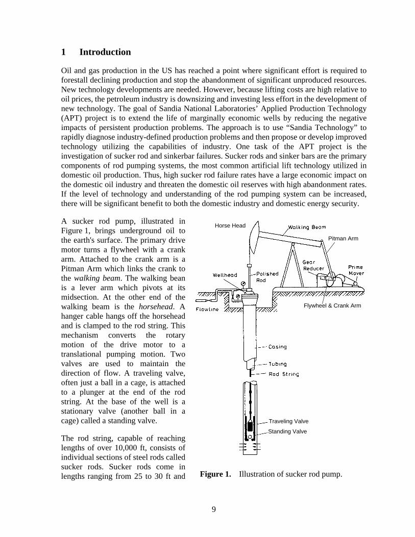
As seen in Figure 13, the inclusion of the Spiralock thread form to the base geometryproduces a significant reduction in the preload of the fully made-up joint, reducing from42 kip to 26 kip. This reduction in the preload is due to a greater amount of yielding of theSpiralock threads relative to the standard API threads. Because the preload is reduced, thecoupling separates at approximately 30 ksi of axial load. The separation is evidenced by thefact that the coupling force goes to zero, while the slope of the pin load plot increases(indicating that the pin is carrying all of the load). The increased load on the pin causes thethreads to yield even further. As stated in the previous section, yielding of the pin threads andshoulder reduces the preload in the coupling. Note that when the load applied to the Spiralockcoupling is returned to zero, the preload is reduced from 15.3 kip to 1.8 kip. The effects ofadding the slimhole or Flexbar modifications to the Spiralock threads is minimal. Theperformance with these additional modifications is nearly identical to the base Spiralockgeometry. These results suggest that the Spiralock thread form requires a greater make-upthan a standard API coupling to achieve the same amount of preload. Figure 14 shows theload plots for the Spiralock coupling (SL) with make-ups of 0.0, 1.0,1.5, 2.0, 2.5, and 3.0. TheSpiralock coupling separates with make-ups of 0.0 and 1.0. Once separation occurs, the pincarries the entire axial load (a maximum 24.1 kip). The 1.5 make-up case experiences agreater amount of thread yielding during the make-up process. As a result, the coupling doesnot separate and a significant amount of the preload is retained after the initial compressionand tension loads (reducing from 20.7 kip to 20.5 kip). While a make-up of 1.5 is sufficient toprevent separation within the load range, a make-up of over 2.0 is required to obtain the sameamount of preload as the fully made-up 7/8-inch API coupling. Further increases in the make-up over 2.0 produce very small increases in the preload. As in the case of the base geometry(see Figure 12), this is due to yielding of the pin shoulder during preload.

29

B

B BB

BB

BB

B

J

J JJ

JJ

JJ

J

H

HH

HH

H

HH

H

EE E E E E EE

E

II I I I I I

I

I

B

B

B

B

B

B

B

B

BJ

J

J

J

J

J

J

J

JH

H

H

H

H

H

H

H

H

I

I

I

II

I

I

I

I

-10000

0

10000

20000

30000

40000

50000

60000

70000

80000

-5000 0 5000 10000 15000 20000 25000 30000 35000 40000

Pin

Lo

ad (

lb)

Axial Load (psi)

cycle 3cycle 1

cycle 2

BBB

B

B

B

B

B

B

JJJ

J

J

J

J

J

J

HHH

HH

H

H

H

H

E

EE

E

E

E

E

E E

II

I

I

I

I

I

I I

B

B

B

B

B

B

B

B

BJ

J

J

J

J

J

J

J

J

H

H

H

H

H

H

H

H

H

IIII

I

I I I I

-80000

-70000

-60000

-50000

-40000

-30000

-20000

-10000

0

10000

-5000 0 5000 10000 15000 20000 25000 30000 35000 40000

Co

up

ling

Fo

rce

(lb

)

Axial Load (psi)

cycle 3cycle 1

cycle 2

Figure 13. Pin load and coupling force as a function of axial load for various combinations of the Flexbar (FB), Spiralock (SL), and slimhole (SH) geometry modifications to the base geometry (S7).

B S7, 1.0 MUJ S7, FB, 1.0 MUH S7, SH, 1.0 MU

S7, SH, FB, 1.0 MUS7, SL, 1.0 MUS7, SL, SH, 1.0 MU

I S7, SL, FB, 1.0 MU

B S7, 1.0 MUJ S7, FB, 1.0 MUH S7, SH, 1.0 MU

S7, SH, FB, 1.0 MUS7, SL, 1.0 MUS7, SL, SH, 1.0 MU

I S7, SL, FB, 1.0 MU

30

B

BB

B B B B B B

J

JJ

J

J

J

J

J J

HH

HH

H

H

H

H

H

BBBB

B

B B B BJJJJ

J

J J J J

H

H

H

H

H

H

H

H

H

-80000

-70000

-60000

-50000

-40000

-30000

-20000

-10000

0

10000

-5000 0 5000 10000 15000 20000 25000 30000 35000 40000

Co

up

ling

Fo

rce

(lb

)

Axial Load (psi)

cycle 3cycle 1

cycle 2

BB BB

B

B

B

B

B

JJ J J J J JJ

J

HH HH

HH

HH

H

B

B

B

B

B

B

B

B

BJ

J

J

J

J

J

J

J

J

H

H

H

H

H

H

H

H

H

-10000

0

10000

20000

30000

40000

50000

60000

70000

80000

-5000 0 5000 10000 15000 20000 25000 30000 35000 40000

Pin

Lo

ad (

lb)

Axial Load (psi)

cycle 3cycle 1

cycle 2

Figure 14. Pin load and coupling force as a function of axial load for the base geometry (S7) with Spiralock threads (SL) and make-ups of 0.0, 1.0,1.5, 2.0, 2.5, and 3.0.

B S7, SL, 0.0 MUJ S7, SL, 1.0 MUH S7, SL, 1.5 MU

S7, SL, 2.0 MUS7, SL, 2.5 MUS7, SL, 3.0 MU

B S7, SL, 0.0 MUJ S7, SL, 1.0 MUH S7, SL, 1.5 MU

S7, SL, 2.0 MUS7, SL, 2.5 MUS7, SL, 3.0 MU

31

3.3 Estimating Fatigue Life of Sucker Rod Couplings

In the previous section, the load distribution in the threaded coupling was discussed in detail.The factors that affect the stress amplitude in the pin under cyclic loading conditions wereexamined. It was mentioned that the fatigue resistance of the coupling would be greatlyimproved if the stress amplitude in the pin were minimized. However, this discussion waspresented in terms of loads and nominal stresses. These nominal stresses can be greatlyaffected by the geometrical features of the coupling, producing stress risers in the couplingwhich will provide preferred sites for crack initiation and growth. In this section, the stressrisers will be identified and the fatigue response at these locations will be characterized foreach of the simulations performed for this study in an attempt to identify features which couldlimit the service life of the coupling.

* SH = slimhole, FB = Flexbar, SL = Spiralock** Maximum load of 40 ksi is 17.7 kip for S6, 24.1 kip for S7, and 31.4 kip for S8

Table 4: Summary of Coupling Performance for Various Analysis Cases

Analysis No

Description*

Initial Preload Preload after Load

Cycle Load Partitioning Factor at

Max Tensile Load**

Load (kip)

Avg Stress (ksi)

Load (kip)

Avg Stress (ksi)

1 S7, 1.0 MU 42.9 50.5 40.1 47.2 0.402

2 S7, 1.5 MU 47.9 56.4 43.8 51.6 0.398

3 S7, 0.0 MU 0.0 0.0 0.0 0.0 1.0

4 S7, FB, 1.0 MU 41.3 48.6 38.4 45.2 0.398

5 S7, SH, 1.0 MU 38.2 45.0 36.0 42.4 0.456

6 S7, SH, FB, 1.0 MU 41.3 48.6 35.3 41.6 0.469

7 S6, 1.0 MU 35.1 53.4 33.8 51.4 0.373

8 S8, 1.0 MU 67.9 57.4 66.0 55.8 0.344

9 S7, FB, SL, 1.0 MU 15.7 18.5 2.6 3.06 1.0

10 S7, SL, SH, 1.0 MU 11.9 14.0 2.8 3.30 1.0

11 S7, SL, 0.0 MU 0.0 0.0 0.0 0.0 1.0

12 S7, SL, 1.0 MU 15.3 18.0 1.8 2.12 1.0

13 S7, SL, 1.5 MU 20.7 24.4 20.5 24.1 0.382

14 S7, SL, 2.0 MU 41.0 48.3 38.2 45.0 0.407

15 S7, SL, 2.5 MU 44.3 52.1 41.8 49.2 0.402

16 S7, SL, 3.0 MU 47.4 55.8 44.0 51.8 0.407

32

3.3.1 Considerations in Life Prediction

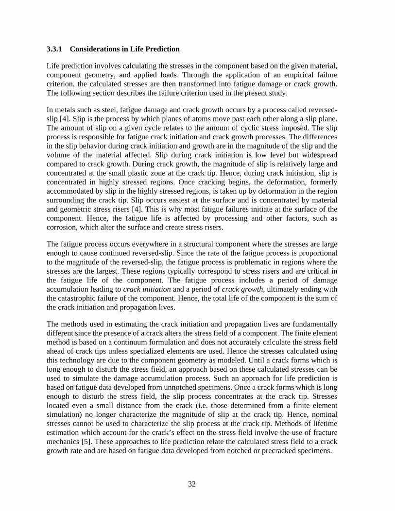
Life prediction involves calculating the stresses in the component based on the given material,component geometry, and applied loads. Through the application of an empirical failurecriterion, the calculated stresses are then transformed into fatigue damage or crack growth.The following section describes the failure criterion used in the present study.

In metals such as steel, fatigue damage and crack growth occurs by a process called reversed-slip [4]. Slip is the process by which planes of atoms move past each other along a slip plane.The amount of slip on a given cycle relates to the amount of cyclic stress imposed. The slipprocess is responsible for fatigue crack initiation and crack growth processes. The differencesin the slip behavior during crack initiation and growth are in the magnitude of the slip and thevolume of the material affected. Slip during crack initiation is low level but widespreadcompared to crack growth. During crack growth, the magnitude of slip is relatively large andconcentrated at the small plastic zone at the crack tip. Hence, during crack initiation, slip isconcentrated in highly stressed regions. Once cracking begins, the deformation, formerlyaccommodated by slip in the highly stressed regions, is taken up by deformation in the regionsurrounding the crack tip. Slip occurs easiest at the surface and is concentrated by materialand geometric stress risers [4]. This is why most fatigue failures initiate at the surface of thecomponent. Hence, the fatigue life is affected by processing and other factors, such ascorrosion, which alter the surface and create stress risers.

The fatigue process occurs everywhere in a structural component where the stresses are largeenough to cause continued reversed-slip. Since the rate of the fatigue process is proportionalto the magnitude of the reversed-slip, the fatigue process is problematic in regions where thestresses are the largest. These regions typically correspond to stress risers and are critical inthe fatigue life of the component. The fatigue process includes a period of damageaccumulation leading to crack initiation and a period of crack growth, ultimately ending withthe catastrophic failure of the component. Hence, the total life of the component is the sum ofthe crack initiation and propagation lives.

The methods used in estimating the crack initiation and propagation lives are fundamentallydifferent since the presence of a crack alters the stress field of a component. The finite elementmethod is based on a continuum formulation and does not accurately calculate the stress fieldahead of crack tips unless specialized elements are used. Hence the stresses calculated usingthis technology are due to the component geometry as modeled. Until a crack forms which islong enough to disturb the stress field, an approach based on these calculated stresses can beused to simulate the damage accumulation process. Such an approach for life prediction isbased on fatigue data developed from unnotched specimens. Once a crack forms which is longenough to disturb the stress field, the slip process concentrates at the crack tip. Stresseslocated even a small distance from the crack (i.e. those determined from a finite elementsimulation) no longer characterize the magnitude of slip at the crack tip. Hence, nominalstresses cannot be used to characterize the slip process at the crack tip. Methods of lifetimeestimation which account for the crack’s effect on the stress field involve the use of fracturemechanics [5]. These approaches to life prediction relate the calculated stress field to a crackgrowth rate and are based on fatigue data developed from notched or precracked specimens.

33

The manufacturers and designers of sucker rod systems exercise extreme care in controllingthe factors which affect the fatigue life of sucker rods. The rods are polished, the specifiedload range accounts for corrosion, and the thread geometry is designed to minimize stressrisers by rounding the root of the threads. As an indication of design intent, sucker rods aresized based on a modified Goodman criteria which ensures an indefinite fatigue life. Hence,this study has taken a conservative approach to lifetime estimation by choosing to apply onlycrack initiation methods to the life estimation of sucker rod couplings. This study neglects thecrack growth life which can contribute a significant number of cycles to the component life.Instead, this study assumes that the coupling has failed once fatigue damage has produced acrack.

As previously stated, crack initiation methods are based on fatigue data developed fromunnotched specimens. In these tests, a specimen is subjected to alternating stresses that varybetween fixed limits of maximum and minimum stress until failure occurs. The load range istypically characterized by a stress ratio, defined as follows:

(13)

Alternatively, the load range is sometimes described in terms of a mean stress and analternating stress, defined as follows:

(14)

(15)

Fatigue tests are repeated for other specimens at the same stress ratio but different stressamplitudes. The results of these tests are plotted to form an S-N diagram. A family of S-Ncurves for a material tested at various stress ratios is shown schematically in Figure 15. In thecase of ferrous metals and alloys, the fatigue strength decreases as the number of cyclesincreases, asymptotically approaching the fatigue limit or endurance limit. If the stressamplitude in a component does not reach the fatigue limit for a given stress ratio, an infinitenumber of load cycles can be applied to the component without causing failure. An endurancelimit does not exist for nonferrous materials. Because S-N curves have this horizontalasymptote, a small change in the stress amplitude can result in a large change in the number ofcycles to failure. Figure 15 also illustrates the effect of stress ratio on the fatigue life andendurance limits. For a given lifetime, as the stress ratio increases, the stress amplitudedecreases. Similarly, the endurance limit decreases as the stress ratio increases. Hence, thefatigue life of a component is effectively reduced by the presence of a mean stress.

The data from S-N curves like that illustrated in Figure 15 can be used to construct a modifiedGoodman diagram. The modified Goodman diagram illustrated in Figure 3 is constructedfrom endurance limit data, hence, providing an indefinite fatigue life. However, a modified

Rσmin

σmax-----------=

σm

σmax σmin+

2------------------------------=

σa

σmax σmin–

2-----------------------------=

34

Goodman diagram can be constructed for any finite life (e.g. 105 cycles). The modifiedGoodman diagram illustrated in Figure 3 exhibits the same dependence on mean stress as theplot in Figure 15. For example, under complete load reversal (R = -1.0), the allowable stressamplitude is T/3. For a fluctuating load (R = 0.0), the allowable stress reduces to T/4. Theallowable stress amplitude (∆σ) continues to decrease up to the limit where the minimum andmaximum stress converge to the ultimate tensile strength of the material. It appears that theallowable stress range adopted by the API (the shaded area in Figure 3) represents aconservative application of the modified Goodman diagram. This conservatism was probablyadopted to ensure that the maximum stress always stay below the yield strength of the suckerrod material (approximately 66 percent of the ultimate tensile strength of API Grade C steel).

3.3.2 Fatigue Damage Criterion for Multiaxial Stress

Nearly all fatigue data is based on uniaxial tests. Under uniaxial conditions, the axial stress,von Mises stress, and maximum principal stress are all equal. Furthermore, the load directionin a uniaxial test never changes throughout the test. Hence, uniaxial test data apply directly tocomponents which are similarly loaded. Since sucker rods are loaded uniaxially, their fatigueperformance can be determined directly from fatigue data. In cases where the component issubjected to a multiaxial stress state, stress measures such as the von Mises stress andmaximum principal stress are not necessarily equal. Hence, an equivalence criteria must bedeveloped to provide a viable basis to relate the multiaxial state of stress being analyzed to thepredominantly uniaxial data which exists in the reference data.

There are two cases of multiaxial stress, referred to as simple and complex multiaxial stress.Simple multiaxial stress refers to the case in which the principal alternating stresses do notchange their direction relative to the stressed part. Complex multiaxial stress refers to the case

Figure 15. Schematic S-N curves for steel at various stress ratios.

Log. lifetime (number of cycles)

Str

ess

Am

plitu

de (

∆σ)

R = 0.0

R = 0.6

R = -1.0

Rσmin

σmax------------=

35

in which the directions of the alternating principal stresses change. The first case can behandled easily by calculating the appropriate equivalent stress [7]. The later case isconsiderably more difficult to analyze and is considered to be beyond the current state oftechnology [4]. Figure 16 shows the maximum principal stress directions in the threads of the7/8-inch API coupling at minimum (-5 ksi) and maximum (40 ksi) loads. The vectors showonly the direction of the maximum principal stress (i.e. the vector lengths are not proportionalto the magnitude of the maximum principal stress). The figure shows that the maximumprincipal stress directions do not change between these extreme loads. In fact, the maximumprincipal stress directions do not change for any of the load steps reported by the simulations.Since the calculations are axisymmetric, the hoop direction is one of the principal stresses andits direction never changes. Since the principal stress directions are orthogonal, it reasons thatthe third principal stress direction does not change either. Hence, sucker rod simulationsrepresent a case of simple multiaxial stress and, as such, can be analyzed with a simpleequivalence criteria.

The present study uses Sines’ method [7,8,9] to determine an equivalent stress for comparisonwith test data. Although no test data exists specifically for API Grade C steel, the method willbe useful in identifying regions with a high potential for crack initiation and to evaluate therelative effects of various design changes on the coupling fatigue life. The method states thatthe permissible effective alternating stress is a linear function of the mean hydrostatic stress.This can be mathematically expressed as follows:

(16)

where σa is the effective alternating stress, is the mean hydrostatic stress,

Figure 16. Maximum principal stress directions in the 7/8-inch API standard coupling at minimum (-5 ksi) and maximum (40 ksi) loads.

σa kσm+ A≤

σm

36

k is a constant specific to the material and fatigue life, andA is the assumed failure criteria.

As long as the left side of Equation (16) is less than the right side, the multiaxial stress statewill not cause failure of the material within the desired life. The constants k and A change withthe assumed fatigue life.

This criterion can be expressed in terms of the principal stresses as follows:

(17)

where Sai = alternating component of the principal stressesSmi = mean component of the principal stressSN = uniaxially fully reversed fatigue stress for N cyclesm = coefficient of mean stress influence

It should be noted that SN is the endurance limit when N approaches infinity. The constants mand SN which describe the fatigue properties for a material can be determined from twofatigue curves in which the stress ratios are appreciably different. Two curves which areconvenient for the determination of these constants are the reversed axial test (R = -1.0) andthe zero-tension fluctuating stress (R = 0.0). In the fully reversed uniaxial test, Equation (17)reduces to:

(18)

verifying that SN is the amplitude of the uniaxial reversed fatigue stress. In the zero-tensionfluctuating stress test, the criterion reduces to:

(19)

where fN is the amplitude of the fluctuating stress (R = 0.0) which would cause failure at thesame lifetime as the reversed stress SN (R = -1.0). Solving the above two equations for myields:

(20)

As previously stated, most fatigue failures initiate at the surface where the stress state isbiaxial. In a biaxial stress state, Equation (17) defines lines of constant von Mises stress whichform ellipses that enclose regions of “safe” alternating stress with respect to a specific fatiguelife. The size of the ellipses varies with the mean stress. As long as the alternating stress (theleft side of Equation (17)) is less than or equal to the “safe” limit (the right side of

Sa1 Sa2–( )2Sa2 Sa3–( )2

Sa3 Sa1–( )2+ +[ ]

1 2⁄

2----------------------------------------------------------------------------------------------------------------- SN m

Sm1 Sm2 Sm3+ +( )3

---------------------------------------------–≤

Sa1 SN=

f N SN mf3---–=

m 3SN

f N------ 1–

=

37

Equation (17)), the multiaxial stress state will not cause failure of the material within thedesired life.

The criterion in Equation (17) can be expressed as a safety factor with respect to the desiredlife, expressed as follows:

(21)

such that when D < 1.0, the stress state will result in a shorter than desired fatigue life. IfD ≥ 1.0, the multiaxial stress state will result in a component life greater than or equal to thatwhich is desired. Equation (21) allows one to determine the “safe” range of the alternatingeffective stress for a given mean hydrostatic stress. If the mean hydrostatic stress is largeenough, making the second term in the numerator larger than the first, D cannot be positive,indicating that there is no “safe” range of alternating stress which will produce the desired life.

It should be emphasized that each fatigue life (specified in number of cycles) will result in anew set of constants, SN and m. Hence, a safety factor can be calculated with respect to anydesired fatigue life. Since the sucker rods are designed for indefinite service, the safety factorcalculated in the present study was with respect to infinite service life. Although there is noknown fatigue threshold data for API Grade C steel, the constants m and SN can beapproximated from the modified Goodman plot shown in Figure 3. Since a safety factor withrespect to failure was desired, the full envelope of the Goodman plot was used to derive theseconstants instead of the more conservative shaded region used by the API. As shown inFigure 3, the amplitude of the reversed stress which will provide an indefinite service life isT/3, whereas the amplitude of fluctuating stress which will provide an indefinite service lifeis T/4. Hence, the constants for API Grade C steel evaluate as follows:

(22)

(23)

Thus, the safety factor with respect to failure can be expressed as:

(24)

with respect to indefinite service life. Because Equation (24) is based on approximateconstants derived from the modified Goodman diagram rather than actual fatigue data, thiscriterion should not be interpreted as predicting failure but rather identifying regions with apotential for fatigue failure. In the case of uniaxial loading, Equation (17) with the constantsSN = 30 ksi and m = 1.0 describes the modified Goodman diagram in Figure 3 in terms ofmean stress and stress amplitude.

DSN mσm–

σa------------------------=

SNT3--- 30ksi= =

m 3 T 3⁄T 4⁄---------- 1–

1.0= =

D30ksi σm–

σa---------------------------=

38

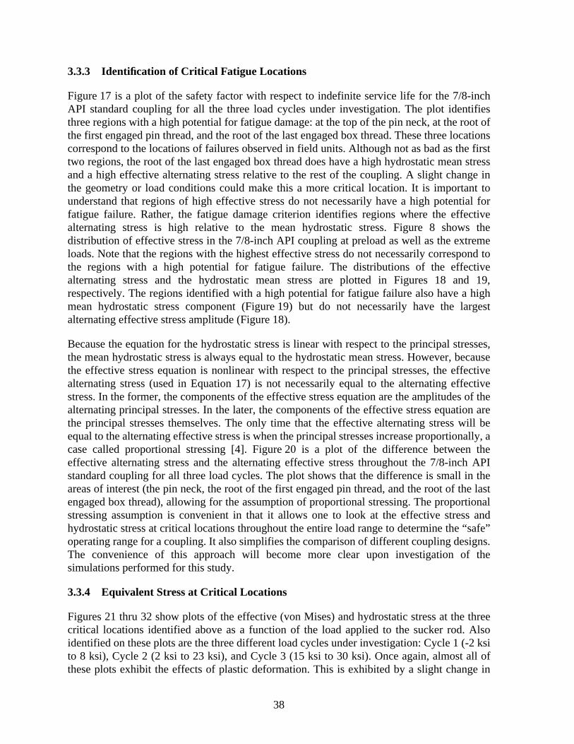
3.3.3 Identification of Critical Fatigue Locations

Figure 17 is a plot of the safety factor with respect to indefinite service life for the 7/8-inchAPI standard coupling for all the three load cycles under investigation. The plot identifiesthree regions with a high potential for fatigue damage: at the top of the pin neck, at the root ofthe first engaged pin thread, and the root of the last engaged box thread. These three locationscorrespond to the locations of failures observed in field units. Although not as bad as the firsttwo regions, the root of the last engaged box thread does have a high hydrostatic mean stressand a high effective alternating stress relative to the rest of the coupling. A slight change inthe geometry or load conditions could make this a more critical location. It is important tounderstand that regions of high effective stress do not necessarily have a high potential forfatigue failure. Rather, the fatigue damage criterion identifies regions where the effectivealternating stress is high relative to the mean hydrostatic stress. Figure 8 shows thedistribution of effective stress in the 7/8-inch API coupling at preload as well as the extremeloads. Note that the regions with the highest effective stress do not necessarily correspond tothe regions with a high potential for fatigue failure. The distributions of the effectivealternating stress and the hydrostatic mean stress are plotted in Figures 18 and 19,respectively. The regions identified with a high potential for fatigue failure also have a highmean hydrostatic stress component (Figure 19) but do not necessarily have the largestalternating effective stress amplitude (Figure 18).

Because the equation for the hydrostatic stress is linear with respect to the principal stresses,the mean hydrostatic stress is always equal to the hydrostatic mean stress. However, becausethe effective stress equation is nonlinear with respect to the principal stresses, the effectivealternating stress (used in Equation 17) is not necessarily equal to the alternating effectivestress. In the former, the components of the effective stress equation are the amplitudes of thealternating principal stresses. In the later, the components of the effective stress equation arethe principal stresses themselves. The only time that the effective alternating stress will beequal to the alternating effective stress is when the principal stresses increase proportionally, acase called proportional stressing [4]. Figure 20 is a plot of the difference between theeffective alternating stress and the alternating effective stress throughout the 7/8-inch APIstandard coupling for all three load cycles. The plot shows that the difference is small in theareas of interest (the pin neck, the root of the first engaged pin thread, and the root of the lastengaged box thread), allowing for the assumption of proportional stressing. The proportionalstressing assumption is convenient in that it allows one to look at the effective stress andhydrostatic stress at critical locations throughout the entire load range to determine the “safe”operating range for a coupling. It also simplifies the comparison of different coupling designs.The convenience of this approach will become more clear upon investigation of thesimulations performed for this study.

3.3.4 Equivalent Stress at Critical Locations

Figures 21 thru 32 show plots of the effective (von Mises) and hydrostatic stress at the threecritical locations identified above as a function of the load applied to the sucker rod. Alsoidentified on these plots are the three different load cycles under investigation: Cycle 1 (-2 ksito 8 ksi), Cycle 2 (2 ksi to 23 ksi), and Cycle 3 (15 ksi to 30 ksi). Once again, almost all ofthese plots exhibit the effects of plastic deformation. This is exhibited by a slight change in

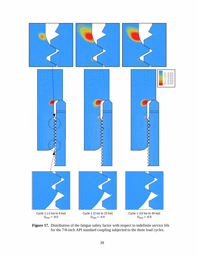
39

Figure 17. Distribution of the fatigue safety factor with respect to indefinite service life for the 7/8-inch API standard coupling subjected to the three load cycles.

Cycle 1 (-2 ksi to 8 ksi)Dmin = -9.0

Cycle 1 (2 ksi to 23 ksi)Dmin = -4.6

Cycle 1 (15 ksi to 30 ksi)Dmin = -6.8

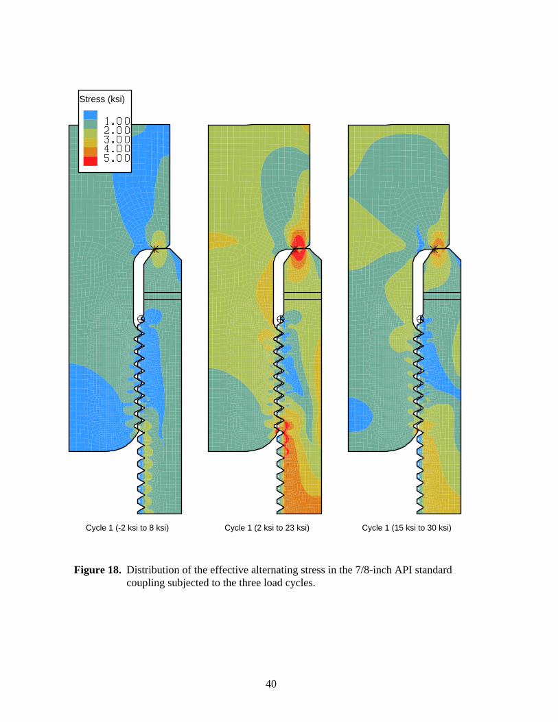
40

Figure 18. Distribution of the effective alternating stress in the 7/8-inch API standard coupling subjected to the three load cycles.

Cycle 1 (-2 ksi to 8 ksi) Cycle 1 (2 ksi to 23 ksi) Cycle 1 (15 ksi to 30 ksi)

Stress (ksi)

41

Figure 19. Distribution of the hydrostatic mean stress in the 7/8-inch API standard coupling subjected to the three load cycles.

Cycle 1 (-2 ksi to 8 ksi) Cycle 1 (2 ksi to 23 ksi) Cycle 1 (15 ksi to 30 ksi)

Stress (ksi)

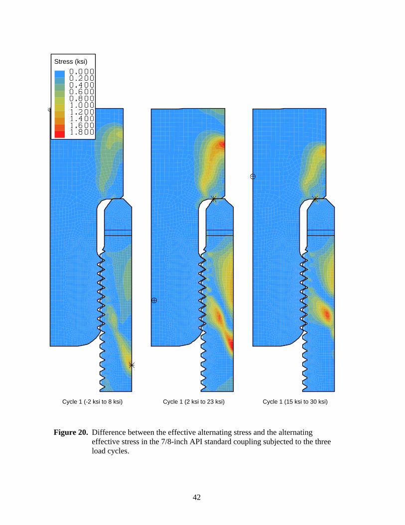
42

Figure 20. Difference between the effective alternating stress and the alternating effective stress in the 7/8-inch API standard coupling subjected to the three load cycles.

Cycle 1 (-2 ksi to 8 ksi) Cycle 1 (2 ksi to 23 ksi) Cycle 1 (15 ksi to 30 ksi)

Stress (ksi)

43

the unloaded state (zero axial load) after the first application of the maximum compressionand tension loads. This is typically due to yielding of the pin shoulder and the threads. Hence,the first application of the maximum compression and tensile loads is identified with a dashedline, while the subsequent applied load cycle is identified by a solid line. Because thenumerator of Equation (24) must be positive in order for there to exist a “safe” range ofalternating stress, the mean hydrostatic stress must be less than the ratio SN/m, which is 30 ksifor API Grade C steel. Hence, for all locations where the hydrostatic stress is greater than30 ksi, there exists no allowable stress range which will produce an indefinite life.

Before considering each case, it is useful to discuss how the information presented in thestress plots in Figures 21 thru 32 can be used by a sucker rod designer. Whereas safety factordistribution plots like that shown in Figure 17 provide a “snapshot” of the fatigue potential fora given load cycle, the stress plots in Figures 21 thru 32 permit in-depth investigation of aninfinite number of load cycles between -5 ksi and 40 ksi. If fatigue data is available, the stressplots can be used to estimate the service life of the coupling. In this case, the constants SN andm from Equation (17) can be calculated for various lifetimes (expressed in number of cycles).The information from the stress plots can then be used to calculate the estimated lifetime ofeach of the three critical locations. Assuming the desired load cycle is known (Cycle 2 forexample), then the mean hydrostatic stress is the value of hydrostatic stress at the middle ofthe cycle (assuming the hydrostatic stress curve is linear over the range of the cycle). Theeffective stress amplitude is one half of the total change in effective stress over the range ofthe cycle. These two values can then be used in Equation (17) with various (SN, m)combinations until the left side of Equation (17) is less than the right. The service lifeassociated with the (SN, m) pair which satisfies the inequality is the approximate service life atthat critical location. The expected coupling life would be the smallest of the estimated livesfor the various critical locations. Alternatively, the sucker rod designer can use the stress plotsto back out the load cycles which will provide a desired service life. In this case, the constants(SN, m) corresponding to the desired service life can be used in Equation (17) to determine theallowable effective stress amplitude for a given mean hydrostatic stress. The designer can thenuse the stress plots to extract the corresponding minimum and maximum loads to be applied tothe sucker rods.

In the absence of fatigue data, the stress plots can be used to compare the relative performanceof various coupling designs and make-ups. This is how the information will be used in thefollowing discussion. Hence, the specific cases are grouped logically to facilitate directcomparison. For a given load cycle, several characteristics of the stress plots providemeaningful information for comparison of the various analysis cases. First, the slope of theeffective stress curve is more significant than the absolute magnitude since the slope isdirectly proportional to the effective stress amplitude over any given load cycle. The greaterthe slope, the higher the effective stress amplitude. Hence, the terms “stress amplitude” and“slope” are used interchangeably in the following discussion of the results. Second, theabsolute magnitude of the hydrostatic stress at the middle of a given load cycle is veryimportant. The smaller the mean hydrostatic stress, the greater the allowable alternatingeffective stress. If, for example, Coupling A has both a higher mean hydrostatic stress and itseffective stress plot has a greater slope (i.e. a higher effective stress amplitude) than CouplingB, then Coupling A will have a shorter service life. It is difficult to assess how much shorter

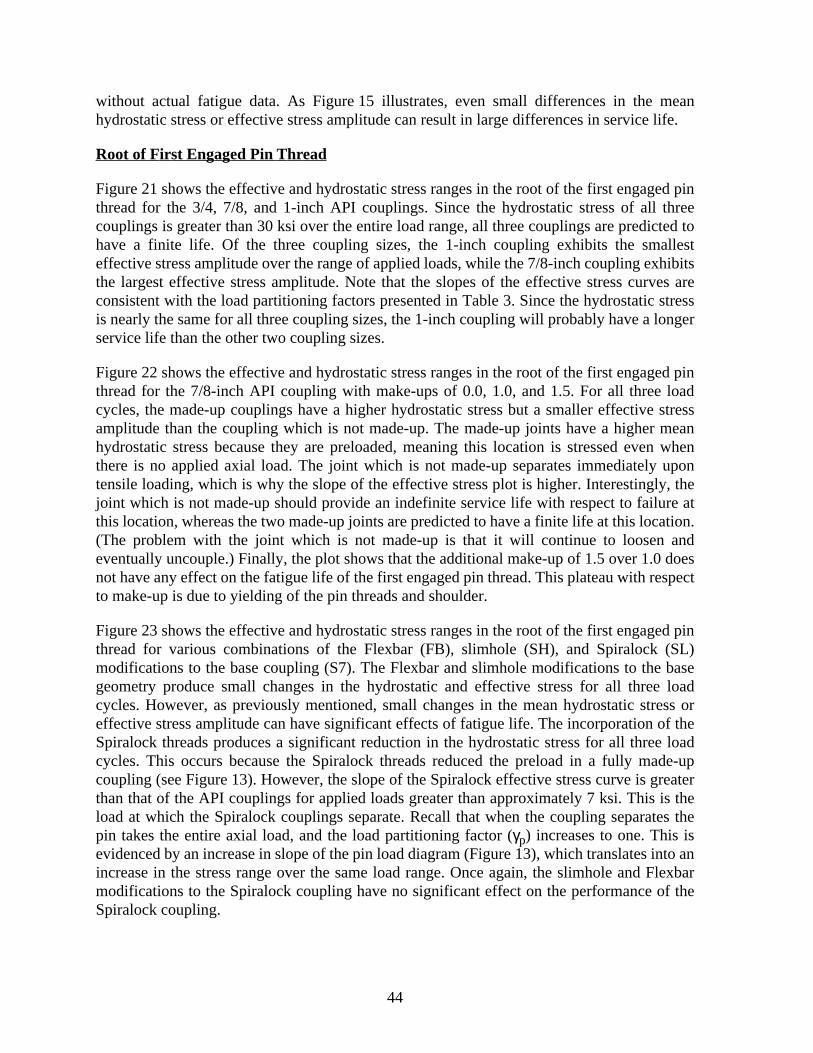
44

without actual fatigue data. As Figure 15 illustrates, even small differences in the meanhydrostatic stress or effective stress amplitude can result in large differences in service life.

Root of Fir st Engaged Pin Thread

Figure 21 shows the effective and hydrostatic stress ranges in the root of the first engaged pinthread for the 3/4, 7/8, and 1-inch API couplings. Since the hydrostatic stress of all threecouplings is greater than 30 ksi over the entire load range, all three couplings are predicted tohave a finite life. Of the three coupling sizes, the 1-inch coupling exhibits the smallesteffective stress amplitude over the range of applied loads, while the 7/8-inch coupling exhibitsthe largest effective stress amplitude. Note that the slopes of the effective stress curves areconsistent with the load partitioning factors presented in Table 3. Since the hydrostatic stressis nearly the same for all three coupling sizes, the 1-inch coupling will probably have a longerservice life than the other two coupling sizes.

Figure 22 shows the effective and hydrostatic stress ranges in the root of the first engaged pinthread for the 7/8-inch API coupling with make-ups of 0.0, 1.0, and 1.5. For all three loadcycles, the made-up couplings have a higher hydrostatic stress but a smaller effective stressamplitude than the coupling which is not made-up. The made-up joints have a higher meanhydrostatic stress because they are preloaded, meaning this location is stressed even whenthere is no applied axial load. The joint which is not made-up separates immediately upontensile loading, which is why the slope of the effective stress plot is higher. Interestingly, thejoint which is not made-up should provide an indefinite service life with respect to failure atthis location, whereas the two made-up joints are predicted to have a finite life at this location.(The problem with the joint which is not made-up is that it will continue to loosen andeventually uncouple.) Finally, the plot shows that the additional make-up of 1.5 over 1.0 doesnot have any effect on the fatigue life of the first engaged pin thread. This plateau with respectto make-up is due to yielding of the pin threads and shoulder.

Figure 23 shows the effective and hydrostatic stress ranges in the root of the first engaged pinthread for various combinations of the Flexbar (FB), slimhole (SH), and Spiralock (SL)modifications to the base coupling (S7). The Flexbar and slimhole modifications to the basegeometry produce small changes in the hydrostatic and effective stress for all three loadcycles. However, as previously mentioned, small changes in the mean hydrostatic stress oreffective stress amplitude can have significant effects of fatigue life. The incorporation of theSpiralock threads produces a significant reduction in the hydrostatic stress for all three loadcycles. This occurs because the Spiralock threads reduced the preload in a fully made-upcoupling (see Figure 13). However, the slope of the Spiralock effective stress curve is greaterthan that of the API couplings for applied loads greater than approximately 7 ksi. This is theload at which the Spiralock couplings separate. Recall that when the coupling separates thepin takes the entire axial load, and the load partitioning factor (γp) increases to one. This isevidenced by an increase in slope of the pin load diagram (Figure 13), which translates into anincrease in the stress range over the same load range. Once again, the slimhole and Flexbarmodifications to the Spiralock coupling have no significant effect on the performance of theSpiralock coupling.

45

Figure 21. Von Mises and hydrostatic stress at the root of the first engaged pin thread as a function of applied axial load for various coupling sizes.

B

B BB

B B B B BJ

J JJ

JJ

J J JHH H H H H H H H

B

B

B

B

B

B

B

B

BJ

J

J

J

J

J

J

J

JH

H

H

H

H

H

H

H

H

-10000

0

10000

20000

30000

40000

50000

60000

-5000 0 5000 10000 15000 20000 25000 30000 35000 40000

Hyd

rost

atic

Str

ess

(psi

)

Axial Load (psi)

Cycle 3

Cycle 2

Cycle 1

B

BB

B

B B B B BJ

JJ

J

J

J

J J JH

HH

H H H H H HB

B

B

B

B

B

B

B

BJ

J

J

J

J

J

J

J

JH

H

H

H

H

H

H

H

H

0

10000

20000

30000

40000

50000

60000

70000

-5000 0 5000 10000 15000 20000 25000 30000 35000 40000

von

Mis

es S

tres

s (p

si)

Axial Load (psi)

Cycle 2

Cycle 1 Cycle 3

B S6, 1.0 MUJ S7, 1.0 MUH S8, 1.0 MU

B S6, 1.0 MUJ S7, 1.0 MUH S8, 1.0 MU

46

Figure 22. Von Mises and hydrostatic stress at the root of the first engaged pin thread as a function of applied axial load for various make-ups of the 7/8-inch API coupling.

BB BB

B

B

B

B

B

J

J JJ

JJ

J J JH

H HH

HH

H H H

B

B

B

B

B

B

B

B

B

J

J

J

J

J

J

J

J

JH

H

H

H

H

H

H

H

H

-10000

0

10000

20000

30000

40000

50000

60000

-5000 0 5000 10000 15000 20000 25000 30000 35000 40000

Hyd

rost

atic

Str

ess

(psi

)

Axial Load (psi)

Cycle 3

Cycle 2

Cycle 1

BB B

B

B

B

B

B

B

J

JJ

J

J

J

J J JH

HH

H

H

H

HH H

B

B

B

B

B

B

B

B

B

J

J

J

J

J

J

J

J

JH

H

H

H

H

H

H

H

H

0

10000

20000

30000

40000

50000

60000

70000

-5000 0 5000 10000 15000 20000 25000 30000 35000 40000

von

Mis

es S

tres

s (p

si)

Axial Load (psi)

Cycle 3Cycle 1

Cycle 2

B S7, 0.0 MUJ S7,1.0 MUH S7, 1.5 MU

B S7, 0.0 MUJ S7,1.0 MUH S7, 1.5 MU

47

Figure 23. Von Mises and hydrostatic stress at the root of the first engaged pin thread as a function of applied axial load for various combinations of the Flexbar (FB), slimhole (SH), and Spiralock (SL) modifications to the base coupling (S7).

B

B BB

BB

B B BJ

J JJ

JJ J J J

H

HH

HH

H H H H

II I I I I I I

I

B

B

B

B

B

B

B

B

BJ

J

J

J

J

J

J

J

JH

H

H

H

H

H

H

H

H

I

I

I

I

I

I

I

I

I

-10000

0

10000

20000

30000

40000

50000

60000

-5000 0 5000 10000 15000 20000 25000 30000 35000 40000

Hyd

rost

atic

Str

ess

(psi

)

Axial Load (psi)

Cycle 3

Cycle 2

Cycle 1

B

BB

B

B

B

B B BJ

JJ

J

J

J J J JH

HH

H

HH H H H

II

I I I I I

I

I

B

B

B

B

B

B

B

B

BJ

J

J

J

J

J

J

J

JH

H

H

H

H

H

H

H

H

I

I

I

I

I

I

I

I

I

0

10000

20000

30000

40000

50000

60000

70000

-5000 0 5000 10000 15000 20000 25000 30000 35000 40000

von

Mis

es S

tres

s (p

si)

Axial Load (psi)

Cycle 1

Cycle 2

Cycle 3

B S7, 1.0 MUJ S7, FB, 1.0 MUH S7, SH, 1.0 MU

S7, SH, FB, 1.0 MUS7, SL, 1.0 MUS7, SL, SH, 1.0 MU

I S7, SL, FB, 1.0 MU

B S7, 1.0 MUJ S7, FB, 1.0 MUH S7, SH, 1.0 MU

S7, SH, FB, 1.0 MUS7, SL, 1.0 MUS7, SL, SH, 1.0 MU

I S7, SL, FB, 1.0 MU

48

Figure 24 shows the effective and hydrostatic stress ranges in the root of the first engaged pinthread of a Spiralock coupling with make-ups of 0.0, 1.0, 1.5, 2.0, 2.5, and 3.0. Again, theeffective stress amplitude increases when the coupling separates (the cases with make-ups of0.0 and 1.0). That is why the slope of the 0.0 and 1.0 make-up curves is larger than those withmake-ups of 1.5 and greater. As the make-up increases above 1.5, the effective stressamplitude over any of the three cycles stays the same (i.e. the slopes of the curves are thesame), while the mean hydrostatic stress increases. This increase in the hydrostatic stress willshorten the service life in this region. Further increases in the make-up over 2.0 produce nosignificant changes in either the effective or hydrostatic stress. This plateau is due to yieldingof the threads during preload. In summary, the Spiralock thread form with a make-up of 1.5appears to offer an improvement over the standard API coupling (1.0 MU) with respect tominimizing both the mean hydrostatic stress and the effective stress amplitude in the root ofthe first engaged thread. This is true for all three load cycles. However, if the coupling is overtightened (make-ups greater than or equal to 2.0), then the performance is very similar to thebase 7/8-inch API coupling.

Pin Neck

All of the above comments made for the stress range in the first engaged pin thread also applyto the plots for the pin neck (Figures 25 thru 28) since the fatigue performance at this locationexhibit the same dependencies on the design parameters. Hence, the discussion of the resultsat this location may seem slightly repetitive. Figure 25 shows the effective and hydrostaticstress ranges in the pin neck for the 3/4, 7/8, and 1-inch API couplings. The effective stressamplitude decreases as the coupling size increases, while the mean stress increases withcoupling size. Once again, note that the slopes of the effective stress curves are consistentwith the load partitioning factors presented in Table 3. Since the mean hydrostatic stress isgreater than 30 ksi over the entire load range, all three coupling sizes are predicted to have afinite life in the pin neck region. Fatigue data would be required to accurately determine thedifferences in fatigue life of the three coupling sizes.

Figure 26 shows the effect of make-up on the stress range in the pin neck. No make-up resultsin the pin carrying the entire axial load. Hence, the effective stress amplitude in the unmade-up coupling is quite large compared to the cases which are made-up. However, make-up hasthe effect of increasing the hydrostatic stress in this region which decreases the fatigue life.The hydrostatic stress of the unmade-up joint is less than 30 ksi over the entire load range.Hence, for every mean stress there exists an alternating effective stress which provideindefinite service life. In the case of the made-up joints, the hydrostatic stress is greater than30 ksi over the entire load range. Hence, both of the made-up joints will have a finite servicelife for any load cycle in this range. Further increases in make-up over 1.0 provide nosignificant change to either the effective stress amplitude or mean hydrostatic stress in the pinneck.

The most effective method for increasing the fatigue life of a component is to decrease theseverity of the stress concentration. The Flexbar modification to the standard API couplingwas designed to decrease the severity of the stress concentration in the pin neck. Figure 27shows that the Flexbar modification reduces both the mean hydrostatic stress and effectivestress amplitude in the pin neck for any of the three cycles. Since the effective stress curve for

49

Figure 24. Von Mises and hydrostatic stress at the root of the first engaged pin thread as a function of applied axial load for the Spiralock coupling with make-ups of 0.0, 1.0, 1.5, 2.0, 2.5, and 3.0.

BB BB

B

B

B

B

B

JJ J J J J J J

J

H

HH

H

HH

HH

H

E

EE

EE E E E EC

CC

CC C C C C

B

B

B

B

B

B

B

B

BJ

J

J

J

J

J

J

J

J

H

H

H

H

H

H

H

H

H

-10000

0

10000

20000

30000

40000

50000

60000

-5000 0 5000 10000 15000 20000 25000 30000 35000 40000

Hyd

rost

atic

Str

ess

(psi

)

Axial Load (psi)

Cycle 3

Cycle 2

Cycle 1

BBB

B

B

B

B

B

B

JJ

JJ J J J

J

J

H

HH

H

H

H

H

H

H

E

EE

E

E E E E EC

CC

C

C C C C C

B

B

B

B

B

B

B

B

BJ

J

J

J

J

J

J

J

J

H

H

H

H

H

H

H

H

H

0

10000

20000

30000

40000

50000

60000

70000

-5000 0 5000 10000 15000 20000 25000 30000 35000 40000

von

Mis

es S

tres

s (p

si)

Axial Load (psi)

Cycle 3Cycle 1

Cycle 2

B S7, SL, 0.0 MUJ S7, SL, 1.0 MUH S7, SL, 1.5 MU

S7, SL, 2.0 MUS7, SL, 2.5 MUS7, SL, 3.0 MU

B S7, SL, 0.0 MUJ S7, SL, 1.0 MUH S7, SL, 1.5 MU

S7, SL, 2.0 MUS7, SL, 2.5 MUS7, SL, 3.0 MU

50

Figure 25. Von Mises and hydrostatic stress at the pin neck as a function of applied axial load for various coupling sizes.

B

B B B B B B B B

J

J J J J J J J J

HH H H HH

HH

H

BB

BB

BB

BB

B

JJ

JJ

JJ

JJ

J

HHHHH H H H H

-10000

0

10000

20000

30000

40000

50000

60000

-5000 0 5000 10000 15000 20000 25000 30000 35000 40000

Hyd

rost

atic

Str

ess

(psi

)

Axial Load (psi)

Cycle 3

Cycle 2

Cycle 1

B

BB

BB B B B BJ

JJ

JJ

J J J JHH H H H H H H HB

B

B

B

B

B

B

B

BJ

J

J

J

J

J

J

J

JH

H

HH

HH

H

H

H

0

10000

20000

30000

40000

50000

60000

70000

-5000 0 5000 10000 15000 20000 25000 30000 35000 40000

von

Mis

es S

tres

s (p

si)

Axial Load (psi)

Cycle 3

Cycle 2

Cycle 1

B S6, 1.0 MUJ S7, 1.0 MUH S8, 1.0 MU

B S6, 1.0 MUJ S7, 1.0 MUH S8, 1.0 MU

51

Figure 26. Von Mises and hydrostatic stress at the pin neck as a function of applied axial load for various make-ups of the 7/8-inch API coupling.

BB B B

B

B

B

B

B

J

J J J J J J J JH

H H H HH H H H

B

B

B

B

B

B

B

B

B

JJ

JJ

JJ

JJ

JH

HH

HH

HH

HH

-10000

0

10000

20000

30000

40000

50000

60000

-5000 0 5000 10000 15000 20000 25000 30000 35000 40000

Hyd

rost

atic

Str

ess

(psi

)

Axial Load (psi)

Cycle 3

Cycle 2

Cycle 1

BB

BB

B

B

B

B

B

J

JJ

JJ

J J J JH

HH

HH

HH H H

B

B

B

B

B

B

B

B

B

J

J

J

J

J

J

J

J

JH

H

H

H

H

H

H

H

H

0

10000

20000

30000

40000

50000

60000

70000

-5000 0 5000 10000 15000 20000 25000 30000 35000 40000

von

Mis

es S

tres

s (p

si)

Axial Load (psi)

Cycle 3

Cycle 2

Cycle 1

B S7, 0.0 MUJ S7,1.0 MUH S7, 1.5 MU

B S7, 0.0 MUJ S7,1.0 MUH S7, 1.5 MU

52

Figure 27. Von Mises and hydrostatic stress at the pin neck as a function of applied axial load for various combinations of the Flexbar (FB), slimhole (SH), and Spiralock (SL) modifications to the base coupling (S7).

B

B B B B B B B BJ

J J J J J J JJH

H H HH H H H H

II II

I

I

II

I

BB

BB

BB

BB

B

JJJJJ J J J JH

H

H

H

H

H

H

H

H

I

I

I

II

I

I

I

I

-10000

0

10000

20000

30000

40000

50000

60000

-5000 0 5000 10000 15000 20000 25000 30000 35000 40000

Hyd

rost

atic

Str

ess

(psi

)

Axial Load (psi)

Cycle 3

Cycle 2

Cycle 1

B

BB

BB

B B B BJ

J J J J J J JJ

H

HH

H

HH H H H

II II

I

I

II

I

B

B

B

B

B

B

B

B

B

JJJJJ J J J J

H

H

H

H

H

H

H

H

H

I

I

I

II

I

I

I

I

0

10000

20000

30000

40000

50000

60000

70000

-5000 0 5000 10000 15000 20000 25000 30000 35000 40000

von

Mis

es S

tres

s (p

si)

Axial Load (psi)

Cycle 3

Cycle 2

Cycle 1

B S7, 1.0 MUJ S7, FB, 1.0 MUH S7, SH, 1.0 MU

S7, SH, FB, 1.0 MUS7, SL, 1.0 MUS7, SL, SH, 1.0 MU

I S7, SL, FB, 1.0 MU

B S7, 1.0 MUJ S7, FB, 1.0 MUH S7, SH, 1.0 MU

S7, SH, FB, 1.0 MUS7, SL, 1.0 MUS7, SL, SH, 1.0 MU

I S7, SL, FB, 1.0 MU

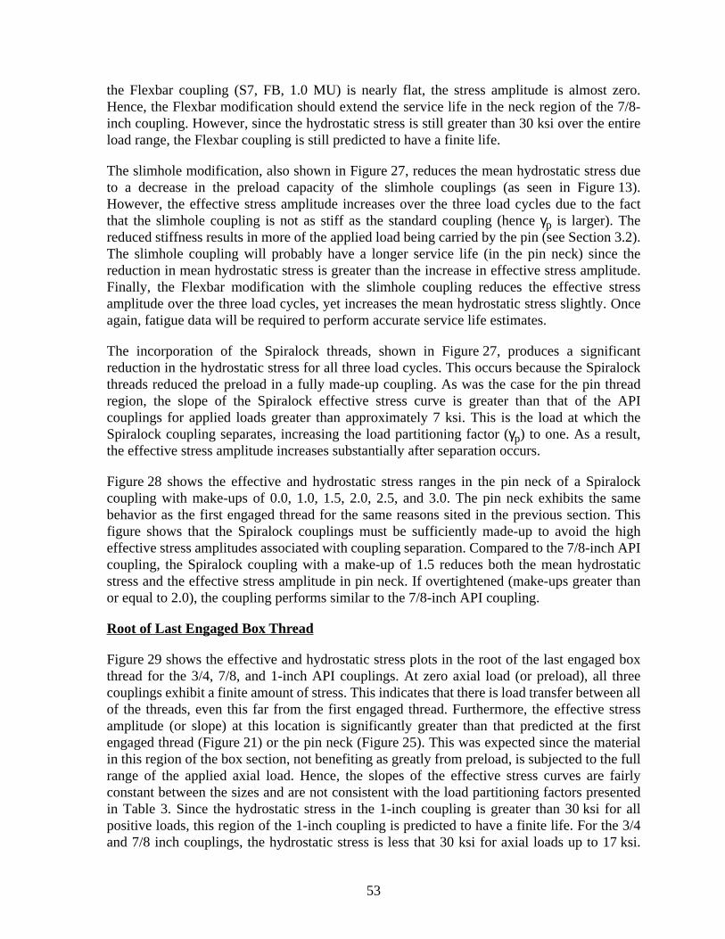
53

the Flexbar coupling (S7, FB, 1.0 MU) is nearly flat, the stress amplitude is almost zero.Hence, the Flexbar modification should extend the service life in the neck region of the 7/8-inch coupling. However, since the hydrostatic stress is still greater than 30 ksi over the entireload range, the Flexbar coupling is still predicted to have a finite life.

The slimhole modification, also shown in Figure 27, reduces the mean hydrostatic stress dueto a decrease in the preload capacity of the slimhole couplings (as seen in Figure 13).However, the effective stress amplitude increases over the three load cycles due to the factthat the slimhole coupling is not as stiff as the standard coupling (hence γp is larger). Thereduced stiffness results in more of the applied load being carried by the pin (see Section 3.2).The slimhole coupling will probably have a longer service life (in the pin neck) since thereduction in mean hydrostatic stress is greater than the increase in effective stress amplitude.Finally, the Flexbar modification with the slimhole coupling reduces the effective stressamplitude over the three load cycles, yet increases the mean hydrostatic stress slightly. Onceagain, fatigue data will be required to perform accurate service life estimates.

The incorporation of the Spiralock threads, shown in Figure 27, produces a significantreduction in the hydrostatic stress for all three load cycles. This occurs because the Spiralockthreads reduced the preload in a fully made-up coupling. As was the case for the pin threadregion, the slope of the Spiralock effective stress curve is greater than that of the APIcouplings for applied loads greater than approximately 7 ksi. This is the load at which theSpiralock coupling separates, increasing the load partitioning factor (γp) to one. As a result,the effective stress amplitude increases substantially after separation occurs.

Figure 28 shows the effective and hydrostatic stress ranges in the pin neck of a Spiralockcoupling with make-ups of 0.0, 1.0, 1.5, 2.0, 2.5, and 3.0. The pin neck exhibits the samebehavior as the first engaged thread for the same reasons sited in the previous section. Thisfigure shows that the Spiralock couplings must be sufficiently made-up to avoid the higheffective stress amplitudes associated with coupling separation. Compared to the 7/8-inch APIcoupling, the Spiralock coupling with a make-up of 1.5 reduces both the mean hydrostaticstress and the effective stress amplitude in pin neck. If overtightened (make-ups greater thanor equal to 2.0), the coupling performs similar to the 7/8-inch API coupling.

Root of Last Engaged Box Thread

Figure 29 shows the effective and hydrostatic stress plots in the root of the last engaged boxthread for the 3/4, 7/8, and 1-inch API couplings. At zero axial load (or preload), all threecouplings exhibit a finite amount of stress. This indicates that there is load transfer between allof the threads, even this far from the first engaged thread. Furthermore, the effective stressamplitude (or slope) at this location is significantly greater than that predicted at the firstengaged thread (Figure 21) or the pin neck (Figure 25). This was expected since the materialin this region of the box section, not benefiting as greatly from preload, is subjected to the fullrange of the applied axial load. Hence, the slopes of the effective stress curves are fairlyconstant between the sizes and are not consistent with the load partitioning factors presentedin Table 3. Since the hydrostatic stress in the 1-inch coupling is greater than 30 ksi for allpositive loads, this region of the 1-inch coupling is predicted to have a finite life. For the 3/4and 7/8 inch couplings, the hydrostatic stress is less that 30 ksi for axial loads up to 17 ksi.

54

Figure 28. Von Mises and hydrostatic stress at the pin neck as a function of applied axial load for the Spiralock coupling with make-ups of 0.0, 1.0, 1.5, 2.0, 2.5, and 3.0.

BB BB

B

B

B

B

B

JJ J JJ

JJ J

J

HH H H H H H HH

E

E E E E E E E E

C

C C C C C C CC

B

B

B

BB

B

B

B

BJ

J

J

JJ

J

J

J

J

HH

HH

HH

HH

H

-10000

0

10000

20000

30000

40000

50000

60000

-5000 0 5000 10000 15000 20000 25000 30000 35000 40000

Hyd

rost

atic

Str

ess

(psi

)

Axial Load (psi)

Cycle 3

Cycle 2

Cycle 1

BB B

B

B

B

B

B

B

JJ J J J J JJ

JHH H

HH

HH

H

H

E

EE

EE E E E EC

CC

CC C C C C

B

B

B

BB

B

B

B

BJ

J

J

JJ

J

J

J

J

H

H

H

H

H

H

H

H

H

0

10000

20000

30000

40000

50000

60000

70000

-5000 0 5000 10000 15000 20000 25000 30000 35000 40000

von

Mis

es S

tres

s (p

si)

Axial Load (psi)

Cycle 3

Cycle 2

Cycle 1

B S7, SL, 0.0 MUJ S7, SL, 1.0 MUH S7, SL, 1.5 MU

S7, SL, 2.0 MUS7, SL, 2.5 MUS7, SL, 3.0 MU

B S7, SL, 0.0 MUJ S7, SL, 1.0 MUH S7, SL, 1.5 MU

S7, SL, 2.0 MUS7, SL, 2.5 MUS7, SL, 3.0 MU

55

Figure 29. Von Mises and hydrostatic stress at the root of the last engaged box thread as a function of applied axial load for various coupling sizes.

B

B

B

B

B

B

B

B

B

J

J

J

J

J

J

J

J

J

H

H

H

H

H

H

H

H

H

B

B

B

B

B

B

B

B

BJ

J

J

J

J

J

J

J

J

H

H

H

H

H

H

H

H

H

-10000

0

10000

20000

30000

40000

50000

60000

-5000 0 5000 10000 15000 20000 25000 30000 35000 40000

Hyd

rost

atic

Str

ess

(psi

)

Axial Load (psi)

Cycle 3

Cycle 2

Cycle 1

B

B

B

B

B

B

B

B

B

J

J

J

J

J

J

J

J

J

HH

H

H

H

H

H

H

H

B

B

B

B

B

B

B

B

BJ

J

J

J

J

J

J

J

J

H

H

H

H

H

H

H

H

H

0

10000

20000

30000

40000

50000

60000

70000

-5000 0 5000 10000 15000 20000 25000 30000 35000 40000

von

Mis

es S

tres

s (p

si)

Axial Load (psi)

Cycle 3

Cycle 2

Cycle 1

B S6, 1.0 MUJ S7, 1.0 MUH S8, 1.0 MU

B S6, 1.0 MUJ S7, 1.0 MUH S8, 1.0 MU

56

Hence, the safety factor (D) will be greater than one in Cycle 1, but less than one for Cycles 2and 3. This is a good example of a marginal region for which the design loads can be tailoredto improve the fatigue life.

Figure 30 shows the stress range in the root of the last engaged box thread for the 7/8-inchAPI coupling with make-ups of 0.0, 1.0, and 1.5. As the plot shows, the made-up couplingshave a greater mean hydrostatic stress than the coupling which is not made-up. However,unlike the first engaged pin thread (Figure 22), the effective stress amplitude in the lastengaged thread is not significantly affected by the amount of preload in the coupling (i.e. theslope does not change much for the made-up couplings). Again, this is due to the fact that thematerial in this region of the box section is subjected to nearly the full range of the appliedaxial load, regardless of the coupling preload. Hence, because preload elevates the mean stressin the last engaged box thread, coupling make-up actually will reduce the fatigue life of thecoupling. Consider Cycle 3 for example, the 7/8-inch API coupling with no make-up willhave a safety factor greater than one, whereas the safety factor drops to less than one with amakeup of 1.0. Again, the problem with no make-up is that the coupling will loosen andeventually separate. Notice that for the made-up joints the effective stress amplitude at the lastengaged box thread is significantly greater than that predicted at the first engaged pin thread(Figure 22) or the pin neck (Figure 26). However, for the coupling which has no make-up, theeffective stress amplitudes in all three locations are nearly equal.

Figure 31 shows the stress range in the root of the last engaged box thread for variouscombinations of the Flexbar (FB), Spiralock (SL), and slimhole (SH) geometry modificationsto the base geometry (S7). The Flexbar modification produces very little change in theeffective stress amplitude or the mean hydrostatic stress for any of the three load cyclesidentified on the plots. This was expected since the Flexbar modification merely increases thegrip length of the coupling, but does not change the thread pattern of the pin and box sections.The largest stress amplitude is predicted for the slimhole couplings. Because the slimholecouplings have a box section with a smaller cross-sectional area, the stress amplitude is largerthan that of the base (S7) coupling. Hence, the stress amplitude in the last engaged thread willalso be larger. In the three Spiralock cases, the mean hydrostatic stress in the last engaged rootthread is significantly smaller than the base (S7) coupling. This is due to the fact that thepreload in these couplings is significantly reduced by thread yielding (see Figure 13).However, the effective stress amplitude is much larger due to the fact that these couplingsseparate at low axial loads (approximately 7 ksi). Once again, in all cases, the effective stressamplitude at the last engaged box thread is greater than that predicted at the first engaged pinthread (Figure 23) or the pin neck (Figure 27) due to the fact that this section of the box issubjected to the full range of the applied load.

Figure 32 shows the stress range in the root of the last engaged box thread for the Spiralockcoupling with make-ups of 0.0, 1.0, 1.5, 2.0, 2.5, and 3.0. The Spiralock coupling separateswith make-ups of 0.0 and 1.0. Once separation occurs, the pin carries the entire axial load.This is evident in Figure 32, where the slope of the stress curve increases at the point at whichseparation occurs. Once again, Figure 32 shows that the Spiralock couplings must besufficiently made-up to avoid the high effective stress amplitudes associated with couplingseparation. Compared to the 7/8-inch API coupling, the Spiralock coupling with a make-up of

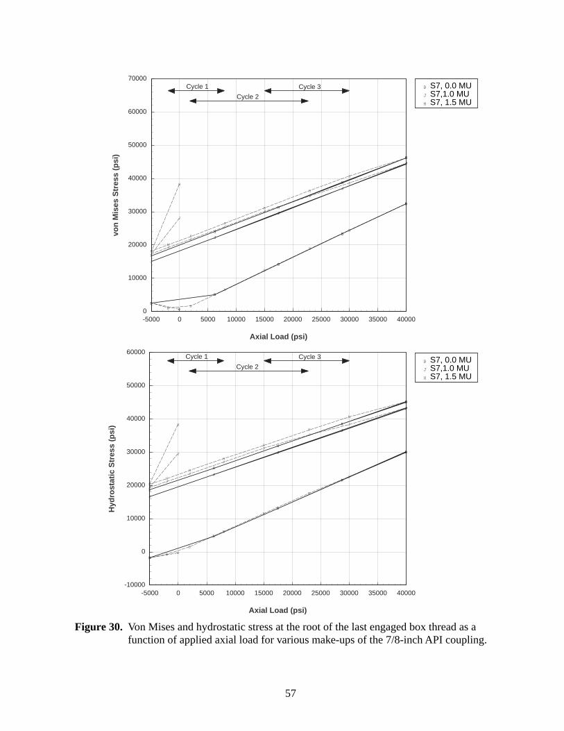
57

Figure 30. Von Mises and hydrostatic stress at the root of the last engaged box thread as a function of applied axial load for various make-ups of the 7/8-inch API coupling.

BB

B

B

B

B

B

B

BJ

J

J

J

J

J

J

J

J

H

H

H

H

H

H

H

H

H

B

B

B

B

B

B

B

B

B

J

J

J

J

J

J

J

J

J

H

H

H

H

H

H

H

H

H

-10000

0

10000

20000

30000

40000

50000

60000

-5000 0 5000 10000 15000 20000 25000 30000 35000 40000

Hyd

rost

atic

Str

ess

(psi

)

Axial Load (psi)

Cycle 3

Cycle 2

Cycle 1

B

BB

B

B

B

B

B

B

J

J

J

J

J

J

J

J

J

H

H

H

H

H

H

H

H

H

B

B

B

B

B

B

B

B

B

J

J

J

J

J

J

J

J

J

H

H

H

H

H

H

H

H

H

0

10000

20000

30000

40000

50000

60000

70000

-5000 0 5000 10000 15000 20000 25000 30000 35000 40000

von

Mis

es S

tres

s (p

si)

Axial Load (psi)

Cycle 3

Cycle 2

Cycle 1

B S7, 0.0 MUJ S7,1.0 MUH S7, 1.5 MU

B S7, 0.0 MUJ S7,1.0 MUH S7, 1.5 MU

58

Figure 31. Von Mises and hydrostatic stress at the root of the last engaged box thread as a function of applied axial load for various combinations of the Flexbar (FB), slimhole (SH), and Spiralock (SL) modifications to the base coupling (S7).

B

B

B

B

B

B

B

B

B

J

J

J

J

J

J

J

J

J

H

H

H

H

H

H

H

H

H

II

II

I

I

I

I

I

B

B

B

B

B

B

B

B

BJ

J

J

J

J

J

J

J

J

H

H

H

H

H

H

H

H

H

I

I

I

I

I

I

I

I

I

-10000

0

10000

20000

30000

40000

50000

60000

-5000 0 5000 10000 15000 20000 25000 30000 35000 40000

Hyd

rost

atic

Str

ess

(psi

)

Axial Load (psi)

Cycle 3

Cycle 2

Cycle 1

B

B

B

B

B

B

B

B

B

J

J

J

J

J

J

J

J

J

H

H

H

H

H

H

H

H

H

II

II

I

I

I

I

I

B

B

B

B

B

B

B

B

B

J

J

J

J

J

J

J

J

J

H

H

H

H

H

H

H

H

H

I

I

I

I

I

I

I

I

I

0

10000

20000

30000

40000

50000

60000

70000

-5000 0 5000 10000 15000 20000 25000 30000 35000 40000

von

Mis

es S

tres

s (p

si)

Axial Load (psi)

Cycle 3

Cycle 2

Cycle 1

B S7, 1.0 MUJ S7, FB, 1.0 MUH S7, SH, 1.0 MU

S7, SH, FB, 1.0 MUS7, SL, 1.0 MUS7, SL, SH, 1.0 MU

I S7, SL, FB, 1.0 MU

B S7, 1.0 MUJ S7, FB, 1.0 MUH S7, SH, 1.0 MU

S7, SH, FB, 1.0 MUS7, SL, 1.0 MUS7, SL, SH, 1.0 MU

I S7, SL, FB, 1.0 MU

59

Figure 32. Von Mises and hydrostatic stress at the root of the last engaged box thread as a function of applied axial load for the Spiralock coupling with make-ups of 0.0, 1.0, 1.5, 2.0, 2.5, and 3.0.

BB

BB

B

B

B

B

B

J

JJ

JJ

J

J

J

J

HH

HH

H

H

H

H

H

EE

E

E

E

E

E

EE

CC

C

C

C

C

C

C C

B

B

B

B

B

B

B

B

BJ

J

J

J

J

J

J

J

JH

H

H

H

H

H

H

H

H

-10000

0

10000

20000

30000

40000

50000

60000

-5000 0 5000 10000 15000 20000 25000 30000 35000 40000

Hyd

rost

atic

Str

ess

(psi

)

Axial Load (psi)

Cycle 3

Cycle 2

Cycle 1

B

B

B B

B

B

B

B

B

J

JJ

J

J

J

J

J

J

HH

H

H

H

H

H

H

H

E

E

E

E

E

E

E

EE

CC

C

C

C

C

C

C C

B

B

B

B

B

B

B

B

BJ

J

J

J

J

J

J

J

JH

H

H

H

H

H

H

H

H

0

10000

20000

30000

40000

50000

60000

70000

-5000 0 5000 10000 15000 20000 25000 30000 35000 40000

von

Mis

es S

tres

s (p

si)

Axial Load (psi)

Cycle 3

Cycle 2

Cycle 1

B S7, SL, 0.0 MUJ S7, SL, 1.0 MUH S7, SL, 1.5 MU

S7, SL, 2.0 MUS7, SL, 2.5 MUS7, SL, 3.0 MU

B S7, SL, 0.0 MUJ S7, SL, 1.0 MUH S7, SL, 1.5 MU

S7, SL, 2.0 MUS7, SL, 2.5 MUS7, SL, 3.0 MU

60

1.5 reduces the mean hydrostatic stress in the last engaged box thread, while the effectivestress amplitude at this location is about the same in both couplings. At higher make-ups (2.0and greater), the mean hydrostatic stress of the Spiralock coupling is still significantly lowerthan that of the API coupling, but the effective stress amplitude is greater.

3.3.5 Effect of Make-up on Service Life

Based on the stress plots presented in the previous section, the Spiralock coupling is predictedto have a longer service life than an equivalent API standard coupling. This longer service lifeis attributed to the lower hydrostatic mean stress throughout the coupling, which is due to areduction in preload for a standard make-up of 1.0. The reduced preload was achievedbecause the Spiralock threads yield more during make-up. As stated previously, the yieldingof the Spiralock threads is due to very localized point contact between the pin and boxthreads. This point contact generates very high stresses in the pin threads, causing them toyield at lower make-ups. Hence, the Spiralock threads function as a preload limiter which willextend the service life of the coupling.

The stress plots for the three critical regions suggest that there is an optimum make-up. Thecouplings must be sufficiently made-up to avoid the high effective stress amplitudesassociated with coupling separation. Yet the couplings should not be overtightened, asadditional make-up increases the mean hydrostatic stress in the coupling which reducesfatigue life. This point was illustrated in the previous section for the Spiralock coupling.Compared to the 7/8-inch API standard coupling, the Spiralock coupling with a make-up of1.5 reduces both the mean hydrostatic stress and the effective stress amplitude at all threecritical locations. If too loose, the coupling separated and the slope of the effective stress plotincreased. If too tight (make-ups greater than or equal to 2.0), the coupling performed similarto the 7/8-inch API coupling. To better illustrate the effect of make-up on fatigue life,Figure 33 shows the distribution of the fatigue safety factor (with respect to indefinite servicelife) in the 7/8-inch Spiralock coupling (with make-ups of 1.0, 1.5, and 2.0) subjected to theentire load range (-5 ksi to 40 ksi). Although the load range is more extreme than sucker rodcouplings are typically subjected to, the plot illustrates that there is an optimum make-upwhich will maximize the fatigue life of a sucker rod coupling. At a make-up of 1.5, the fatigueaffected regions are small and the minimum safety factor is 0.8. If too loose (1.0 MU), theaffected regions increase in size and the minimum safety factor decreases to 0.7. If thecoupling is too tight (2.0 MU), the affected regions increase in size and the minimum safetyfactor decreases to -2.1 (the negative implies there is no “safe” amplitude of effective stress).Hence, the optimum make-up is that which is just enough to avoid coupling separation duringthe desired load cycle. From a practical standpoint, the make-up should be increased slightlyabove this point so that the coupling will not loosen and uncouple.

The above discussion suggests that the sucker rod designer can maximize the service life of arod string by controlling the preload achieved during make-up. The Spiralock couplingpartially achieves this by using a thread design that yields during make-up. Even with theSpiralock threads, there is an optimum make-up (approximately 1.5) which should not beexceeded. The difference in make-ups of 1.5 and 2.0 is only 9/64-inch of circumferentialdisplacement, little more than one tenth of an inch. Hence, the fatigue life of a sucker rodcoupling is very sensitive to the amount of circumferential displacement. From a practical

61

Figure 33. Fatigue safety factor distribution in the 7/8-inch Spiralock coupling (with make-ups of 1.0, 1.5, and 2.0) subjected to the full axial load range (-5 ksi to 40 ksi).

S7, SL, 1.0 MUDmin = 0.7

S7, SL, 1.5 MUDmin = 0.8

S7, SL, 2.0 MUDmin = -2.1

62

standpoint, it is unreasonable to expect field workers to make-up joints within such tolerances.Even if they could, the Spiralock coupling has another disadvantage. If the coupling isreworked (disassembled and then reassembled), the threads will not yield as much on thesecond make-up (due to work hardening of the threads) and the preload in the coupling willincrease. Hence, the circumferential displacement required to achieve a given preload of theSpiralock coupling will change with each rework. This will be true of any coupling whichyields during make-up. A more repeatable solution for controlling coupling preload could beobtained by using crushable steel washers between the box and the pin shoulder. The highstrength steel used for the pin and box sections is necessary for fatigue resistance. A steelwasher would be necessary to maintain the coupling stiffness. However, a much lowerstrength steel could be used for the washer since in is always loaded in compression, and,therefore, does not need to be fatigue resistant. The lower yield strength washer will result in aconstant crush force for a fairly wide range of circumferential displacements. This way, thecoupling preload would not be particularly sensitive to the circumferential displacement. Sucha design would allow the optimum preload to be achieved with current API thread forms.Furthermore, the washers could be discarded and replaced should the coupling need to bereworked.

63

4 Conclusions and Recommendations

The response of a variety of sucker rod couplings to an applied axial load was simulated usingaxisymmetric finite element models. The sucker rod geometries included the 3/4, 7/8, and 1-inch API (American Petroleum Institute) standard couplings. Various combinations of theslimhole, Spiralock, and Flexbar modifications to the 7/8-inch coupling were investigated,resulting in a total of nine simulated geometries. In addition, the effect of various make-ups(assembly tightness) on the performance of the 7/8-inch API standard and 7/8-inch Spiralockcouplings was investigated, resulting in a total of 16 simulations. The make-up process, basedon measured circumferential displacement of the coupling from a hand-tight position, wassimulated by including a section of an axially expanding material in the box section which,when heated, produced the desired mechanical interference which would result from making-up of the coupling. After make-up, an axial load was applied to the sucker rod ranging from -5 ksi to 40 ksi, encompassing three load cycles identified on a modified Goodman diagram asacceptable for indefinite service life of the sucker rods. Two cycles of the -5 ksi to 40 ksi loadcycle were applied to assure that the coupling response was elastic. The constitutive responseof the API Grade C steel to the applied loads included both elastic and plastic response.

All of the simulations exhibited some yielding during the make-up process and in the firstapplication of the maximum compression and tensile loads, generally in the pin neck,shoulder, and threads. Yielding on the first load cycle reduced the preload in the couplingwhich was obtained after make-up. Hence, the preload in a given coupling is a function of theextreme loads it is subjected to. After the initial yielding during make-up and in the firstcompression and tension cycles, the coupling responds elastically throughout the entire loadcycle. Although the sucker rod stresses were, by design, within the envelope of the modifiedGoodman diagram, the local stresses in the couplings were clearly outside of this envelope forall three load cycles, indicating that all of the simulated couplings would have a finite life.

The simulations of the various coupling geometries and make-ups were compared withrespect to how well they accomplish the two primary objectives of preloading threadedcouplings: (1) to lock the threaded coupling together so that it will not loosen and eventuallyuncouple, and (2) to improve the fatigue resistance of the threaded connection by reducing thestress amplitude in the coupling when subjected to cyclic loading. Evaluation of the firstobjective, locking the threaded coupling, was relatively simple. A coupling will remain lockedas long as the mating surfaces of the pin and box sections remain in compression, resistingrotational motion or loosening. Determining how well the various couplings satisfy the secondobjective, fatigue resistance, was considerably more difficult. This evaluation wasaccomplished in two parts: nominally and locally. In the nominal evaluation, a set ofequations based on the gross dimensions of the coupling were derived which describe how aload applied to a sucker rod is distributed throughout a preloaded coupling. A percentage ofthe load reduces the compression between the pin and box sections, while remainder increasesthe tension in the pin section. The later portion, termed the pin partitioning factor, isproportional to the stiffness of the box section of the coupling. A smaller pin partitioningfactor reduces the nominal stress amplitude in the pin section and, hence, improves its fatigueresistance. Once a coupling separates, all of the applied load is carried by the pin and the pinpartitioning factor increases to a maximum of one. Hence, fatigue resistance is maximized if

64

the coupling remains locked. The relative stiffness of the pin and box sections is, in general,proportional to their cross-sectional areas. The results of the finite element simulations, interms of nominal load distribution, agreed well with the nominal load distribution equations.

The local fatigue evaluation characterized the fatigue performance of the various couplingsusing the local stresses predicted in the finite element simulations and a stress equivalencingcriterion for multiaxial stress states. This criterion is based on Sines’ equivalent stress theorywhich states that the permissible effective alternating stress is a linear function of the meanhydrostatic stress. The fatigue damage criterion identified three locations with a high potentialfor fatigue failure: the pin neck, the root of the first engaged pin thread, and the root of the lastengaged box thread. All three locations correspond to the locations of failures observed infield units. Perhaps the most significant finding in this part of the study was thecharacterization of the coupling parameters which affect the two controlling stress measuresof the fatigue criterion. The mean hydrostatic stress, which determines the permissibleeffective alternating stress, is a function of the coupling make-up. Whereas, the effectivealternating stress is a function of the relative stiffness of the pin and box sections of thecoupling. As long as the coupling does not separate, the alternating effective stress isunaffected by the amount of circumferential displacement applied during make-up. The localand nominal evaluations were consistent in that the local effective alternating stressamplitudes were proportional to the pin load partitioning factors calculated using the nominalstress equations. These findings suggest three approaches to improving the fatigue resistanceof sucker rod couplings.

• Decrease the nominal alternating stress amplitude by increasing the box stiffness relativeto the pin stiffness. This could be accomplished by either increasing the outside diameterof the box section or by decreasing the pin diameter. The later approach could be taken ininstances where well bore clearance is tight. In addition to reducing the nominal stressamplitudes in the pin, a larger box cross-section will reduce the nominal stress amplitudenear the last engaged box thread. Demonstrating the effects of relative stiffness, theslimhole coupling, which has a smaller diameter box section, is less stiff than the standardAPI coupling. As a result, the finite element simulations exhibited a larger nominal loadamplitude in the slimhole coupling as well as larger local alternating effective stresses.

• Optimize the preload generated during the make-up process to minimize the local meanhydrostatic stress in the coupling. The preload in a coupling needs to be large enough tolock the coupling and avoid the high effective stress amplitudes associated with couplingseparation. Additional preload serves only to increase the local mean hydrostatic stressesand decrease the service life of the coupling. The Spiralock coupling partiallyaccomplishes this optimization by incorporating a thread design which yields extensivelyduring make-up, reducing the preload generated in a standard API make-up. As a result,the local mean hydrostatic stresses are considerably smaller in the Spiralock coupling thanthey are in the API coupling. The analyses demonstrated that the optimum make-up for theSpiralock coupling was approximately one and a half times the standard API make-up.Hence, achievement of an optimum preload still depends on assembler skill. Perhaps amore effective and repeatable method for controlling preload would be to use a crushablesteel washer between the pin and box sections.

65

• Decrease the severity of the stress concentrations which provide preferred sites for fatiguedamage. This approach was taken in designing the Flexbar modification to the standardAPI coupling. The results of the Flexbar simulations indicate that this modification wassuccessful in reducing both the mean hydrostatic and effective alternating stresses in thepin neck, extending the service life of the coupling with respect to failure at this location.

Any combination of the above design approaches could be used to extend the service lives ofexisting sucker rod couplings, or to design a coupling which would meet the desiredrequirement of indefinite service life.

The local fatigue damage criterion used in this study provided a format for identifying regionswith a high potential for fatigue damage and for comparing the fatigue performance of thevarious coupling geometries and make-ups. If fatigue data was available, this local fatiguedamage criterion could have been used to perform service life estimates of the variouscouplings and make-ups. Consideration should be given to performing multiaxial fatigue testswhich could validate this criterion and be used to estimate service lives of sucker rodcouplings.

References1 J. H. Biffle, M. L. Blanford, “JAC2D — A Two-Dimensional Finite Element Computer

Program for the Nonlinear Quasi-Static Response of Solids with the Conjugate Gradi-ent Method,” Internal Report SAND93-1891, Sandia National Laboratories, Albuquer-que, NM, May 1994.

2 J. W. Waggoner, R. G. Buchheit, “Analysis of Sucker Rod and Sinkerbar Failures,”Southwestern Petroleum Short Course, pp.124-141, 1993.

3 J. E. Shigley and L. D. Mitchell, “Mechanical Engineering Design,” Fourth Edition,McGraw Hill, New York, 1983.

4 “Fatigue Design Handbook,” Second Edition, Society of Automotive Engineers, 1988.

5 J. M. Barsom and S. T. Rolfe, “Fracture and Fatigue Control in Structures, Applicationsof Fracture Mechanics,” Second Edition, Prentice-Hall, Inc., 1987.

6 H. E. Boyer, “Atlas of Fatigue Curves,” American Society for Metals, 1986.

7 H. O. Fuchs and R. I. Stephens, “Metal Fatigue in Engineering,” John Wiley & Sons,1980.

8 G. Sines, “Metal Fatigue,” McGraw-Hill, 1959.

9 G. Sines, “Failure of Metals Under Combined Repeated Stresses with SuperimposedStatic Stresses,” NACA Tech. Note 3495, 1955.

66

DistributionMS0328 2674 C. F. Briner

MS0899 4916 Technical Library

MS0701 6100 R. W. Lynch

MS0705 6116 R. P. Cutler (100)

MS0705 6116 M. C. Walck

MS9018 8940-2 Central Technical Files

MS0841 9100 P. J. Hommert

MS0841 9101 T. C. Bickel

MS0833 9103 J. H. Biffle (Route to 9111 & 9115)

MS0834 9112 A. C. Ratzel (Route to 9112 & 9113)

MS0836 9116 C. W. Peterson (Route to 9114 & 9116)

MS0443 9117 J. G. Arguello

MS0443 9117 S. N. Burchett

MS0443 9117 E. L. Hoffman (10)

MS0443 9117 H. S. Morgan (Route to 9117 & 9118)

MS0443 9117 C. M. Stone

MS0443 9117 G. W. Wellman

MS0443 9117 QA File

MS0437 9118 C. R. Adams

MS0828 9104 R. K. Thomas

MS0439 9234 D. R. Martinez (Route to staff)

MS0619 12690 Review and Approval Desk for DOE/OSTI