Sampling theory - CBS Netherlands Statistics Methods (201207) Sampling theory Sampling design and...

Statistics Netherlands

Statistics Methods (201207)

Sampling theory

Sampling design and estimation methods

The Hague/Heerlen, 2012

112Reinder Banning, Astrea Camstra and Paul Knottnerus

Explanation of symbols

. data not available

* provisional � gure

** revised provisional � gure (but not de� nite)

x publication prohibited (con� dential � gure)

– nil

– (between two � gures) inclusive

0 (0.0) less than half of unit concerned

empty cell not applicable

2011–2012 2011 to 2012 inclusive

2011/2012 average for 2011 up to and including 2012

2011/’12 crop year, � nancial year, school year etc. beginning in 2011 and ending in 2012

2009/’10–2011/’12 crop year, � nancial year, etc. 2009/’10 to 2011/’12 inclusive

Due to rounding, some totals may not correspond with the sum of the separate � gures.

PublisherStatistics NetherlandsHenri Faasdreef 3122492 JP The Hague

Prepress Statistics NetherlandsGrafimedia

CoverTeldesign, Rotterdam

InformationTelephone +31 88 570 70 70Telefax +31 70 337 59 94Via contact form: www.cbs.nl/information

Where to orderE-mail: [email protected] +31 45 570 62 68

Internetwww.cbs.nl

ISSN: 1876-0333

© Statistics Netherlands, The Hague/Heerlen, 2012.Reproduction is permitted, provided Statistics Netherlands is quoted as source.

60165201207 X-37

3

Contents

1. Introduction to the subthemes ............................................................................4

2. Simple random sampling without replacement ..................................................6

3. Stratified samples .............................................................................................17

4. Cluster sampling, Two-stage sampling and Systematic sampling ...................30

5. Samples with equal and unequal inclusion probabilities..................................53

6. Ratio estimator .................................................................................................67

7. Regression estimator ........................................................................................75

8. Poststratified estimators ...................................................................................81

9. References........................................................................................................86

4

1. Introduction to the subthemes

1.1 General description

This document describes various sampling designs and estimation methods used at

Statistics Netherlands. The main focus is on random samples, in which units are

selected from the population according to a well defined selection mechanism.

The most straightforward and familiar procedure is simple random sampling without

replacement (SRSWOR), in which each possible sample (of equal size) from the

population has exactly the same chance of selection. Simple random sampling is the

basic selection method, and all other random sampling techniques can be viewed as

an extension or adaptation of this method. These other, more complex, designs

generally aim to increase the efficiency, i.e. to improve the estimates, but practical

and economic considerations can also play a part in choosing a design. However, in

all types of sampling, each element of the target population must have a positive and

known probability of being included in the sample, which is referred to as the

inclusion probability.

Having chosen a sampling design, it must be determined how to estimate the

population parameters of interest, such as a population total or a poplation mean.

The choice of a specific estimating method is largely determined by the presence of

auxiliary information and the nature of the relationship between the target variable

and the auxiliary information. Accordingly, a quotient estimator, regression

estimator or poststratification estimator may be selected.

The ‘Sampling design’ subtheme is covered in Chapters 2, 3, 4 and 5. The

‘Estimation methods’ subtheme is covered in Chapters 6, 7 and 8. Furthermore,

equations and formulas are numbered to facilitate referencing from elsewhere in the

text. Equation numbers are marked with an asterisk (*) to indicate that a proof is

provided in the appendix to the chapter concerned.

1.2 Scope and relationship with other themes

There is clearly a relationship between estimation and weighting to adjust for

nonresponse. The methods and techniques discussed under that subject build upon

the elementary estimation methods discussed in this document, but are oriented

more to the problem of nonresponse.

There is also a relationship with the Panels theme, in which population elements are

incorporated into the sample in the course of several consecutive observation

periods. This approach is often used when the interest is in trends over time. There

are also clear relationships with the theme Experiments and the theme Model-based

Estimation as, for example, applied to small subpopulations.

5

1.3 Place in the statistical process

It will be clear from the above that the sampling design is relevant at the start of the

statistical process, whereas estimation occurs more towards the end, shortly before

the figures are published.

6

2. Simple random sampling without replacement

2.1 Short description

Simple random sampling without replacement (SRSWOR) is the most familiar

sampling design. This kind of sampling is referred to as simple because it involves

drawing from the entire population. Alternatively, simple random sampling can be

carried out with replacement (SRSWR), but this type of design is not used at

Statistics Netherlands. However, since the relatively simple SRSWR variance

formulas can be used under certain conditions in SRSWOR, SRSWR and the

associated variance formulas will be briefly discussed in Section 2.3.3.

2.1.1 Definition of SRSWOR

The rather formal definition of SRSWOR is as follows. Consider a population U of

N elements, or },,2,1{ NU L= . SRSWOR is a method of selecting n elements out of

U such that all possible subsets of U of size n have the same probability of being

drawn as a sample. Note that there are

n

N possible subsets of U of size n.

2.1.2 Sampling scheme for SRSWOR

In practice SRSWOR can involve successively selecting random numbers between

1 and N, and including each associated population element in the sample until n

elements have been selected. If a number is already drawn, a new number is selected

at random. A good alternative to SRSWOR is systematic sampling, which is defined

in Section 4.3.3.

2.2 Applicability

Statistics Netherlands applies SRSWOR mainly for business statistics. The

population of businesses is usually stratified and SRSWOR is performed for each

stratum – see the next chapter for stratified sampling. The SRSWOR design is also

frequently used as a sort of benchmark to evaluate other sampling designs by

comparing the variances of the different design based estimators.

2.3 Detailed description

2.3.1 Assumptions and notation

We start with a short description of a number of important population parameters.

Given a specific target variable we distinguish the population total Y, the

population mean Y , the population variance 2yσ , the adjusted population variance

2yS , and the population coefficient of variation yCV . The adjusted population

variance is often used to simplify the SRSWOR formulas. Moreover, kY stands for

7

the value of the target variable of element k , Nk ,,1 L= . The stated parameters are

defined as follows:

.

)(1

1

1

)(1

11

1

222

1

22

1

11

Y

SCV

YYNN

NS

YYN

YN

YN

Y

YYYY

yy

N

kkyy

N

kky

N

kk

N

kkN

=

−−

=−

=

−=

==

=++=

∑

∑

∑

∑

=

=

=

=

σ

σ

L

(2.1)

The n (i.e. the sample size) observations of the target variable in the sample are

denoted in small letters .,,1 nyy L The sample mean sy , the sample variance 2ys

and the sample coefficient of variation ycv are the three most important sample

parameters. These three sample parameters are defined as follows:

( )

.

11

1

1

22

1

s

yy

n

ksky

n

kks

y

scv

yyn

s

yn

y

=

−−

=

=

∑

∑

=

=

(2.2)

2.3.2 Estimators for the population mean, population total and adjusted population

variance

For three of the five population parameters defined in (2.1) explicit estimators are

formulated below. These parameters are the population total, the population mean

and the adjusted population variance. Intuitively, the sample mean sy seems a

reasonable estimator of the population mean. It is denoted as follows:

∑=

==n

kks y

nyY

1

1ˆ (2.3)

The hat ^ on the left-hand side indicates an estimator of the corresponding

parameter.

The estimator of the population mean leads to the following proposal for the

estimator of the population total:

∑=

===

n

kks y

n

NyNYNY

1

ˆˆ (2.4)

The parameter nN / in this expression is referred to as the inclusion weight of the

sample because it gives the ratio of population size to sample size.

8

Finally, we present the sample variance as the estimator of the adjusted population

variance, i.e.:

( )∑=

−−

==n

kskyy yy

nsS

1

222

1

1ˆ . (2.5)

The unbiasedness of the estimators

An estimator is unbiased if its expected value is equal to the statistic to be estimated.

In order to determine the expectations of the (direct) estimators for the population

mean and population total in SRSWOR, it is convenient to write the estimators in an

alternative form. The estimator for the population mean is rewritten as:

∑=

==N

kkks Ya

nyY

1

1ˆ (2.6)

where the binary random variable ka is defined as:

=samplein theincludediselement if0

samplein theincludediselement if1

notk

kak (2.7)

The binary random variable ka is also known as the selection indicator. The

selection indicator has the following two favourable properties:

,N,kN

naPaE kk L1)1()( ==== (2.8)

and:

( ) ( )( )

≤≠≤−

−

=∧==

.11

1

,,1

NlkNN

nn

NklkN

n

aaE lk

L(2.9)

Take the alternative expression (2.6) for the estimator of the population mean as

starting point. Then it can be demonstrated from properties (2.8) and (2.9) of

selection indicator ka that this estimator is an unbiased estimator of Y :

( ) ( )

.11

11ˆ

11

11

YYN

YN

n

n

YaEn

Yan

EYE

N

kk

N

kk

N

kkk

N

kkk

===

=

=

∑∑

∑∑

==

==

With this result it is also simple to verify that the estimator of the population total is

unbiased, i.e.:

( ) ( ) ( ) .ˆˆˆ YYNYENYNEYE ====

9

The selection indicators are also useful in proving that 2ys in (2.5) is an unbiased

estimator of the adjusted population variance. In other words:

( ) ( ) .1

1 2

1

22y

n

ksky Syy

nEsE =

−−

= ∑=

(2.10*)

The asterisk (*) alongside the number of the above equation indicates that a proof is

given in the appendix to this chapter.

Variance calculations

It can be proved that the variance of the estimator of population mean is a function

of the adjusted population variance:

( ) .11

11ˆvar 22

=

−=−=

N

nfS

f

f

NSf

nY yy (2.11*)

The factor )1( f− is referred to as the finite population correction, while the factor f

is referred to as the sampling fraction. Based on this result, the variance of the

estimator of the population total is:

( ) .1ˆvarˆvar 22

ySf

fNYNY

−=

= (2.12)

The value of parameter f is plotted against the value of parameter ff /)1( − in

Figure 2.1. If with (fixed) population size N, the sample size n increases in value,

the sampling fraction f becomes 1. Reading from the graph, parameter ff /)1( −

then approaches 0. In other words, the variance of the estimator of population total

approaches 0 as the sample becomes larger – see expression (2.12).

The variance of the estimator of the population mean, as calculated in (2.11), can be

estimated using the following estimator:

( ) 11ˆ11ˆrav 22yy s

f

f

NS

f

f

NY

−=

−= (2.13)

where 2ys represents the sample variance. The unbiasedness of this variance

estimator follows from that of the sample variance 2ys as an estimator of adjusted

population variance .2yS

An unbiased estimate of the variance of estimator Y , as calculated in (2.12) can be

calculated similarly using the estimator

( ) 1ˆrav 2ys

f

fNY

−= (2.14)

10

with 2ys the sample variance. The unbiasedness of this variance estimator is a direct

consequence of the (proven) unbiasedness of 2ys as an estimator of .2

yS

Figure 2.1. Parameter f plotted against parameter ff /)1( −

0.0 0.2 0.4 0.6 0.8 1.0

05

1015

2025

3035

f

(1−

f)f

Coefficients of variation

Besides calculating (and estimating) an estimator’s variance, it is also possible to

determine the associated coefficient of variation. The coefficients of variation of the

estimator of the population mean, denoted as ( )YCV ˆ , and the estimator for the

population total, denoted as ( )YCV ˆ , are defined as follows:

( ) ( )( )

.ˆvar

)ˆ(

ˆvarˆ

Y

YYCV

Y

YYCV

=

=(2.15)

Formula (2.11) gives an expression for the variance of the estimator of the

population mean under SRSWOR. This formula can be used to derive the equation

below, from which the coefficient of variation of the estimator can be calculated

( ) 22 11ˆyCV

f

f

NYCV

−

= . (2.16)

11

In other words, there is a direct relationship between the coefficient of variation of

the estimator of the population mean and the population coefficient of variation.

Given the relationship between the population total and the population mean, and

the relationship between the estimator of the population mean and the estimator of

the population total, it is possible to demonstrate that the coefficients of variation of

the two estimators are related as follows:

( )

= YCVYCV ˆˆ (2.17)

This equation expresses that the direct estimators of the population total and the

population mean are equally accurate.

Unfortunately it is impossible to actually calculate the two coefficients of variation

in (2.15), and consequently they have to be estimated. The obvious estimator for the

coefficient of variation of the estimator of the population mean is:

( )

−

=

f

f

Ny

sYVC

s

y 11ˆˆ (2.18)

because:

.ˆs

yyy y

scvVC ==

It is important to note that the sampling fraction is often very small in practice, i.e.

0≈f . In fact, this is then equivalent to random sampling with replacement. It is

also intuitively clear that replacement or non replacement no longer has an effect on

the value of the estimator when the population size is much greater than the sample

size. The next subsection discusses simple random sampling with replacement.

2.3.3 Simple random sampling with replacement

Suppose that we perform simple random sampling with replacement with equal

drawing probabilities N/1 (SRSWR). Then nyy ,,1 L can be viewed as n

independent selections from NYY ,,1 L , with the following expectation and variance:

( ) nkYYN

yEN

llk ,,1

1

1

L=== ∑=

and:

( ) ( ) .,,11

var 2

1

2nkYY

Ny y

N

llk L==−= ∑

=

σ (2.19)

Note that these two formulas also apply to SRSWOR. In the SRSWR case, these

two formulas directly lead to the expectation and the variance, respectively, of the

estimator syY =ˆ :

12

( ) ( )∑=

==n

kks YyE

nyE

1

1

and:

( ) .1

var 2ys n

y σ= (2.20*)

Comparing the variance formulas in this subsection with those in the previous

subsection confirms the property mentioned above that the variance formulas are

approximately the same for small f.

Finally, note that in SRSWR .)( 22yysE σ= The proof is largely the same as for

SRSWOR, and is therefore omitted.

2.3.4 Determination of sample size

A frequently asked question in practice is how large a sample has to be to make

inferences, with a certain accuracy, about Y , the population total. A commonly used

criterion for accuracy is the 95% confidence interval )(95 YI . The definition of

)(95 YI is that there is a 95% probability of the unknown population total falling

within )(95 YI . Assuming that the statistic Y is approximately normally distributed,

an approximate value of the 95% confidence interval for Y for sufficiently large n is:

( ) ( ) .ˆrav96.1ˆ,ˆrav96.1ˆ)(95

+−= YYYYYI

Using percentage margins of uncertainty, this expression can also be formulated as:

( )

( ) .%196ˆˆˆ

%100ˆ

ˆrav96.1ˆ)(95

×±=

±=

YVCY

Y

YYYI

(2.21)

This is explained below with reference to a simple example. Assume 120ˆ =Y and

( ) .25ˆrav =Y We then obtain ).8.129;2.110()8.9120;8.9120()(95 =+−=YI In

accordance with (2.21) we can also express this interval as %.2.8120 ±

The above equations also allow determination of the sample size that would be

needed in order to remain within a given margin of uncertainty, say %r . From

rf

f

NCVy <

−× 11196

it follows that:

.196

196222

22

fCVrN

CV

y

y <×+×

×

If a 5% margin of uncertainty is considered acceptable, the sampling fraction f for a

population with 000,1=N and a 7.0=yCV must satisfy the following inequality:

13

.43.049.019625000,1

49.0196min2

2

ff <=≈×+×

×

For the given population size 000,1=N , this minimum sampling fraction

corresponds to a minimum sample size of 430min =n .

Needless to say, in practice yCV must first be estimated in some way. The estimate

can often be based on recent past data. Sometimes it is also possible to use

comparable data with the same volatility.

2.4 Example: estimating fractions

If we wish to calculate the percentage of people with a certain attribute, e.g. the

number of people with a high salary, kY will assume the following values:

.,,1salaryhigh ahavenot doesperson if0

salaryhigh ahasperson if1Nk

k

kYk L=

=

If YP = is the fraction of high-salary earners in the population, then (N.B. in this

situation kk YY =2 ):

( )

.1

)1(11

1

2

2

1

22

1

22

1

PQN

NS

PQPQPPPYN

PYN

PYN

Y

y

N

kk

N

kky

N

kk

−=

−==−=−=−=

==

∑∑

∑

==

=

σ

The sampling fraction of high-salary earners is Pp ˆ= , in accordance with formulas

(2.3) and (2.11):

( ) .1

1

111var 2 PQ

f

f

NS

f

f

Np

yp

y

s

−

−=

−=

=

The latter result, the calculated variance of the estimator, can be estimated with

(2.13):

( )

( ) ( ) .11

11

1

11111)r(av

1

22

ppn

f

pynf

f

Ns

f

f

Np

n

kky

−

−−=

−

−

−=

−= ∑=

The coefficient of variation of estimator p can therefore be estimated as follows –

see (2.15) and also (2.18):

( ) ( ) .1

1

11ˆ

−

−−=

p

p

nfpVC

14

It follows from formula (2.21) for the 95% confidence interval p that for sufficiently

large n , )(95 pI can be estimated as:

( ) .1

1

11%196)(95

−

−−×±=

p

p

nfpPI

The above formula states that the relative margin of uncertainty increases strongly

with decreasing p. For example, if on the basis of SRSWOR parameter P is

estimated at 001.0 with 000,50=n , then assuming that 0≈f , the relative margin

of uncertainty is %28 . This illustrates the difficulty of estimating what are known

as small domains with sufficient accuracy.

2.5 Quality indicators

The quality indicators for SRSWOR are:

- the margins of uncertainty of the corresponding estimators;

- the size of nonresponse.

Nonresponse can severely affect the quality of the results if (i) the nonresponse is

large and (ii) the nonresponse is selective. The bias from selective nonresponse can

sometimes be corrected by using auxiliary variables that correspond with both the

probability of response and the target variable.

Another important assumption in random sampling is that the frame from which the

sample is drawn corresponds closely with the target population about which

inferences are to be made.

2.6 Appendix

Proof of (2.10)

Before deriving a formula for the variance of estimator (2.3), it is pointed out that

the variance of the estimator for the population mean does not change if we add a

constant to all kY in the population. In other words, it may be assumed without loss

of generality of the results that the population mean is zero, i.e. 0=Y . Based on this

assumption, we rewrite the expression for sample variance using the selection

indicator as:

.11

1

11

1 2

1

22

1

22s

N

kkks

n

kky y

n

nYa

ny

n

ny

ns

−−

−=

−−

−= ∑∑

==

The expectation 2ys can be calculated from definitions (2.2) and (2.6) as (N.B.

)var()( 2ss yyE = because 0=Y ):

15

( ) ( ) ( )

( )

.ˆvar11

var11

1

111

2

1

2

2

1

22

−−

−=

−−×

−=

−−

−=

∑

∑

=

=

Yn

n

n

n

yn

nY

N

n

n

yEn

nYaE

nsE

y

s

N

kk

s

N

kkky

σ

In other words, the expectation of the sample variance is a function of the variance

of the estimator of the population mean. Calculating the expectation of the sample

variance therefore requires knowledge of the variance of the estimator of the

population mean. In (2.11) a formula for the variance of the estimator of the

population mean is derived.

Using the above result and expression (2.11) gives:

( ) ( )( )( ) ( )

.

11

1

11

11

2

22

222

y

yy

yyy

S

SnN

nNS

nN

Nn

Sfnn

n

n

nsE

=−

−−−−=

−×−

−−

= σ

Therefore 2ys is an unbiased estimator of 2

yS . QED.

Proof of (2.11)

We make the same simplifying assumption in proving formula (2.11) for the

variance of the sample mean as before, i.e. that .0== YY It follows from (2.7) –

(2.9) that:

( ) ( )

.11

1

1

11

1

1

1

)0()1(

)1(1

1

1ˆˆvar

2

2

2

222

11

2

2

1 11

222

2

1

2

y

y

y

yy

N

kkk

N

kk

N

k

N

kll

lklk

N

kkk

N

kkk

Sf

f

N

SN

N

N

nN

n

N

N

N

nN

n

N

n

n

n

YYNN

nnY

N

n

n

YYaaEYaEn

Yan

EYEY

−=

−×−−××=

−−=

−−−=

−−

−+=

+=

=

=

∑∑

∑∑∑

∑

==

=≠==

=

σ

σσ

Expression (2.11) for the variance of the sample mean is therefore correct. QED.

16

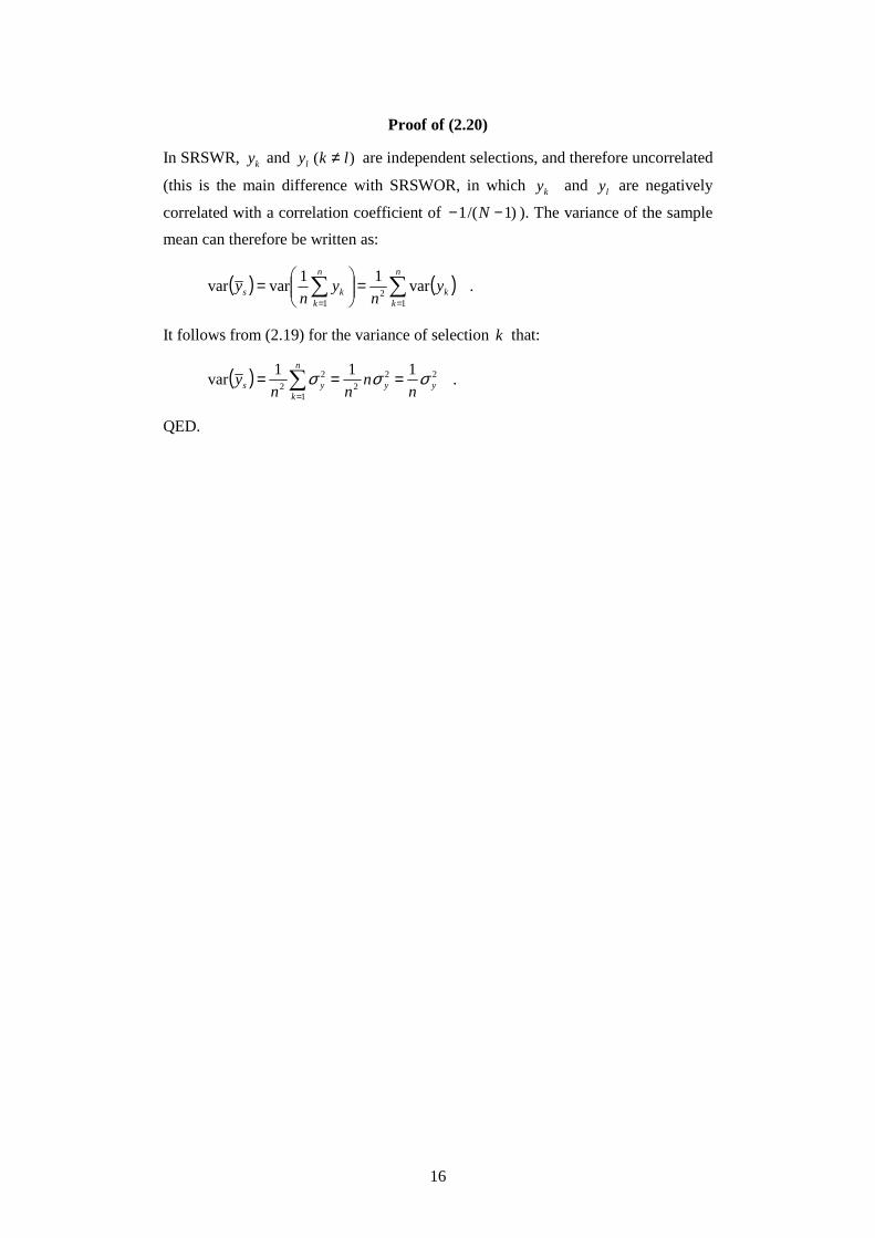
Proof of (2.20)

In SRSWR, ky and )( lkyl ≠ are independent selections, and therefore uncorrelated

(this is the main difference with SRSWOR, in which ky and ly are negatively

correlated with a correlation coefficient of )1/(1 −− N ). The variance of the sample

mean can therefore be written as:

( ) ( ) .var11

varvar1

21

∑∑==

=

=n

kk

n

kks y

ny

ny

It follows from (2.19) for the variance of selection k that:

( ) .111

var 222

1

22 yy

n

kys n

nnn

y σσσ === ∑=

QED.

17

3. Stratified samples


The definition of a stratified random sample assumes division of the target

population into what are known as strata (the singular form is stratum). The strata

must be nonoverlapping and together they must cover the whole population. A

random sample is then selected from every stratum by SRSWOR. The different

SRSWOR samples are mutually independent. In other words, rather than having one

large SRSWOR selection, SRSWOR is performed in several smaller steps.

3.2 Applicability

Statistics Netherlands often uses regional, demographic, or socioeconomic factors

for stratification. Stratification, i.e. dividing the target population into strata,

requires the necessary auxiliary information to be available in the sampling frame.

For example, to stratify according to branch of industry, this information must be

known for each company in the sampling frame. The General Business Register

contains a company’s standard industrial classification and size category, which are

auxiliary variables that Statistics Netherlands often uses for stratification. The

information for every person in the Municipal Personal Records Database (GBA)

includes much personal data, such as gender, date of birth, marital status and

address, which can be used to categorize the Dutch population.

Stratified random sampling can be used for a variety of reasons. First, stratification

is a common way of improving the precision of estimators (i.e. to reduce the

variance), in particular when estimating characteristics of the entire population.

Some variables, e.g. company revenue, can have such a large population variance

that very large samples are needed to make reliable inferences. If it is possible to

form groups within which the target variable varies little, stratified sampling can

lead to more precise outcomes than simple random sampling (with equal sample

size). Precision improves because the variance within the strata is less than the

variance for the population as a whole.

Second, the interest is often not only in the population as a whole, but also in

specific subpopulations or in making comparisons between subpopulations. In

simple random sampling, it is a matter of chance how many elements end up in the

strata. Small subpopulations in particular will then be poorly represented in the

sample. Stratification is a way of ensuring that all subpopulations of interest are

sufficiently represented in the sample to allow reliable statements to be made.

Third, it is possible in stratification to use different data collection techniques for

different strata. For instance, it may be desirable in a business survey to approach

small companies by means of a brief paper questionnaire and to have large

companies take part in an extensive telephone or personal interview. The selection

and estimating methods may also differ for each stratum.

18

Fourth, for administrative reasons, sampling frames are often already divided into

‘natural’ parts, which may even be kept at geographically different locations. In this

case separate sampling may be more economical.



The population is divided into H strata. An individual stratum is denoted with the

index Hhh ,,1, L= , and comprises hN elements. The strata must not overlap. In

other words, each element must belong to exactly one stratum. The strata jointly

form the population, so that

NNH

hh =∑

=1

where again N is the total population size. We also assume that the size hN of every

stratum is known. The value of the target variable of element k in stratum h is

denoted with hkY , for Hh ,,1 L= , and hNk ,,1 L= . The sample size of stratum h is

expressed as hn ; by definition nnh h =∑ . The notation for the sample observations

in stratum h is hky , with Hh ,,1L= , and hnk ,,1 L= .

For a target variable we distinguish the following stratum parameters: the stratum

total hY , the stratum mean hY , the stratum variance 2yhσ , the adjusted stratum

variance 2yhS , and the coefficient of stratum variation yhCV . These parameters are

defined as follows:

( )

( )

.

1

1

1

1

1

22

1

22

1

h

yhyh

N

khhk

hyh

N

khhk

hyh

hh

h

N

khkh

Y

SCV

YYN

S

YYN

YN

Y

YY

h

h

h

=

−−

=

−=

=

=

∑

∑

∑

=

=

=

σ (3.1)

N.B. the above parameters refer to population parameters in stratum h.

Because a stratified sampling design involves taking a sample in each stratum, the

sample parameters are discussed per stratum. The sample parameters in a stratum

are: the sample mean hy in stratum h, the sample variance 2yhs in stratum h, and the

sample coefficient of variation yhcv in stratum h. They are defined as follows:

19

( )

.

11

1

1

22

1

h

yhyh

n

khhk

hyh

n

khk

hh

y

scv

yyn

s

yn

y

h

h

=

−−

=

=

∑

∑

=

=

(3.2)

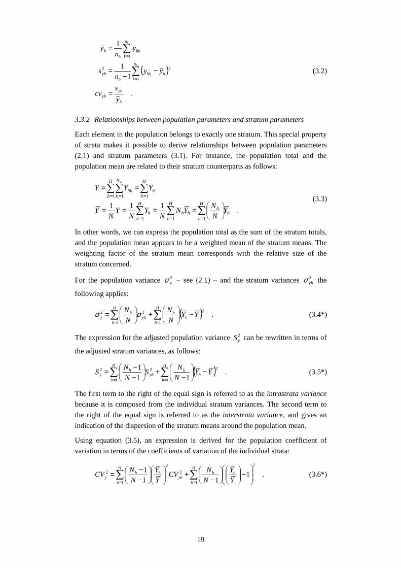
3.3.2 Relationships between population parameters and stratum parameters

Each element in the population belongs to exactly one stratum. This special property

of strata makes it possible to derive relationships between population parameters

(2.1) and stratum parameters (3.1). For instance, the population total and the

population mean are related to their stratum counterparts as follows:

.111

111

11 1

∑∑∑

∑∑∑

===

== =

====

==

H

hh

hH

hhh

H

hh

H

hh

H

h

N

khk

YN

NYN

NY

NY

NY

YYYh

(3.3)

In other words, we can express the population total as the sum of the stratum totals,

and the population mean appears to be a weighted mean of the stratum means. The

weighting factor of the stratum mean corresponds with the relative size of the

stratum concerned.

For the population variance 2yσ – see (2.1) – and the stratum variances 2

yhσ the

following applies:

( ) .1

2

1

22 ∑∑==

−

+

=

H

hh

hH

hyh

hy YY

N

N

N

N σσ (3.4*)

The expression for the adjusted population variance 2yS can be rewritten in terms of

the adjusted stratum variances, as follows:

( ) .11

1

1

2

1

22 ∑∑==

−

−+

−−=

H

hh

hH

hyh

hy YY

N

NS

N

NS (3.5*)

The first term to the right of the equal sign is referred to as the intrastrata variance

because it is composed from the individual stratum variances. The second term to

the right of the equal sign is referred to as the interstrata variance, and gives an

indication of the dispersion of the stratum means around the population mean.

Using equation (3.5), an expression is derived for the population coefficient of

variation in terms of the coefficients of variation of the individual strata:

.111

1

1

2

1

2

2

2 ∑∑==

−

−+

−−=

H

h

hhH

hyh

hhy Y

Y

N

NCV

Y

Y

N

NCV (3.6*)

20

3.3.3 Estimators of population mean and population total

SRSWOR is performed separately for each stratum in the stratified sample. That is,

from the population of hN elements in a stratum h, we perform SRSWOR to select

a sample of size hn . Estimators of stratum mean and then stratum total are directly

available (see e.g. Chapter 2):

.ˆ

ˆ

hhh

hh

yNY

yY

=

=(3.7)

These two estimators will be used in estimating the population total and population

mean.

The population total Y corresponds with the sum of the stratum totals hY , see (3.3).

It is therefore logical to estimate the population total by means of estimators of the

stratum totals. An estimator of this kind that explicitly uses the stratification design

is referred to as a stratification estimator. The stratification estimator of the

population total, denoted as STY , is therefore by definition:

∑∑==

==H

hhh

H

hhST yNYY

11

ˆˆ . (3.8)

By analogy the stratification estimator of the population mean, denoted as STY , is

defined as:

∑=

==

H

hh

hSTST y

N

NY

NY

1

ˆ1ˆ . (3.9)

To recap, both the population total and population mean can be estimated with a

weighted sum of the stratum means. The respective stratum-dependent weighting

factors are the absolute stratum size and the relative stratum size.


SRSWOR is performed for each stratum to select a sample of size hn . This type of

random sample has several known properties – see Chapter 2. Accordingly, the

estimators of the stratum mean and stratum total – see (3.7) – can be taken to be

unbiased. Given the unbiasedness of the estimator of the stratum total, it is possible

to calculate the expected value of the stratification estimator for the population total

(3.8):

( ) ( ) .ˆˆ11

YYYEYEH

hh

H

hhST === ∑∑

==

The stratification estimator (3.8) is therefore an unbiased estimator of the population

total. We use this result in calculating the expected value of the stratification

estimator of the population mean:

21

( ) ( ) .1ˆ1ˆ YYN

YEN

YE STST ===

This demonstrates that STY is an unbiased estimator of the population mean.

The proofs for the unbiasedness (i.e. the formal derivations of the calculated

expected values) of estimators (3.8) and (3.9) given above confirm what is clear

intuitively. The fact is that if the estimators of the stratum totals are unbiased, then

the weighted sum of the estimators of the stratum totals is also unbiased. Identical

reasoning applies to the estimators of the stratum means and the weighted sum of

the estimators of the stratum means.


The variance of, for example, the estimator of the stratum total, can also be

determined directly – see expression (2.12):

( ) .1ˆvar 2

yhh

hhyh S

f

fNY

−= (3.10)

In this formula hf is the sampling ratio in stratum h, i.e. hhh Nnf /= . SRSWOR is

performed independently in the various strata of the stratified sample. Consequently

the variance of the stratification estimator of the population total equals the sum of

the variances of the individual estimators of the stratum totals. That is,

( ) ( ) .1ˆvarˆvar 2

11yh

H

h

h

h

hH

hhST S

N

N

f

fNYY ∑∑

==

−== (3.11)

Using (3.11) and the natural relationship between the stratification estimators of the

population mean and population total, the variance of the stratification estimator of

the population mean can be calculated as:

( ) ( ) .11ˆvar

1ˆvar1

22 ∑

=

−==H

hyh

h

h

hSTST S

N

N

f

f

NY

NY (3.12)

Further inspection of formulas (3.11) and (3.12) reveals that both variances are

small if and only if the individual adjusted stratum variances 2yhS are small. Small

adjusted stratum variance means that the target variable varies little within the

stratum, or in other words that the stratum is internally homogeneous. The variance

of the estimator also appears to depend on the allocation scheme used, since the

individual adjusted stratum variances depend on the size of the random samples.

The variance of the stratification estimator of the population total – see (3.10) – is a

weighted linear combination of the adjusted stratum variances. An estimator of this

variance can therefore be obtained by estimating each individual adjusted stratum

variance. The sample variance in SRSWOR is known to be an unbiased estimator of

the adjusted population variance. Using this result we obtain:

22

( ) .1ˆ1ˆrav

1

2

1

2 ∑∑==

−=

−=

H

hyh

h

h

hH

hyh

h

h

hST s

N

N

f

fNS

N

N

f

fNY (3.13)

By analogy the variance of the stratification estimator of the population mean can be

estimated as follows:

( ) .11ˆrav

1ˆrav1

2

2 ∑=

−==

H

hyh

h

h

hSTST s

N

N

f

f

NY

NY (3.14)

Because the sample variance is an unbiased estimator of the adjusted population

variance in SRSWOR – see formula (2.10) – we know that estimators (3.13) and

(3.14) are unbiased.

Coefficients of variation

Analogous to definition (2.15), the coefficients of variation of the stratification

estimators of the population total and population mean, are defined by:

( ) ( )

.

ˆvarˆ

ˆvarˆ

Y

YYCV

Y

YYCV

ST

ST

STST

=

=

(3.15)

It can be established from formulas (3.11) and (3.12) that the above coefficients of

variation are equal:

( ) ( )( ) ( ) .ˆ

ˆvarˆvar

ˆ1

1

ST

N

STNST

ST YCVY

Y

Y

YYCV ==

=

The stratification estimators of the population total and population mean are

therefore equally accurate.

Expression (3.11) is used in determining )ˆ( STYCV . The result can be rewritten in

terms of the stratum coefficients of variation – see definition (3.1). After squaring,

we obtain the following relationship between the coefficient of variation of the

stratification estimator of the population mean, and the individual stratum

coefficients of variation:

( ) .1ˆ

1

2

2

2 ∑=

−=

N

hyh

hh

h

hST CV

Y

Y

N

N

f

fNYCV

3.3.4 Sampling design evaluation

The principal idea of stratified sampling designs is that stratification yields a more

precise estimator than simple random sampling. If the observations within the strata

are generally more homogeneous than in the the population as a whole, the reduced

variance in the strata will lead to a smaller variance of the estimator.

23

Sampling designs can be evaluated by comparing the variance of an estimator for a

particular design with the variance of the corresponding estimator based on a

SRSWOR sample of equal size (which is also known as the SRSWOR estimator).

The ratio of the two variances is known as the design effect, or DEFF. The design

effect for the stratification estimators of the population total and population mean,

respectively, are defined (under the necessary condition that 0)ˆvar( ≠EAZTY ) as:

[ ] ( )( )

[ ] ( )( ) .ˆvar

ˆvarˆ

ˆvar

ˆvarˆ

SRSWOR

STST

SRSWOR

STST

Y

YYDEFF

Y

YYDEFF

=

=

(3.16)

A DEFF value of 1 indicates that the variances of the two estimators are equal; the

precision of the stratification estimator is then the same as that of the SRSWOR

estimator. Mutatis mutandis, a stratified random sample is more efficient than a

SRSWOR sample of the same size if DEFF is less than 1, and less efficient if

DEFF is greater than 1. The actual calculation of a design effect requires explicit

calculations of both variances.

The design effect for the stratification estimator of the population mean can be

calculated as follows:

( ) ( )( ) ( ) [ ] .ˆ

ˆvar

ˆvar

ˆvar

ˆvarˆ

2

2

1

1

ST

SRSWORN

STN

SRSWOR

ST

ST YDEFFY

Y

Y

YYDEFF ==

=

In other words, the design effects for the stratification estimators of the population

total and population mean are equal. With hindsight this is not surprising because

the design effect is actually no more than the ratio of the squares of the coefficients

of variation of the stratification estimator and the SRSWOR estimator.

A compact expression for the design effect of the stratification estimator of the

population total can be derived if a simple relationship exists between )ˆvar( STY and

)ˆvar( SRSWORY . Unfortunately, there is no relationship of this kind for the general

case. However, a relationship does exist under two, not particularly strict,

conditions.

Assume for the remainder of the discussion in this subsection that the sampling ratio

hf is constant. This assumption simplifies equation (3.11) as follows:

( ) .11ˆvar

1

2

1

2 ∑∑==

−=

−=H

hyh

hH

hyh

h

h

hST S

N

N

f

fNS

N

N

f

fNY (3.17)

The variance of the SRSWOR estimator of the population total, based on a sample

of the same size, depends on the adjusted population variance 2yS – see (2.12).

Therefore assume in the second instance that the following conditions are fulfilled:

24

( ) ( ) .11 −≈∧−≈ NNNN hh (3.18)

Based on this assumption the expression for )ˆvar( SRSWORY can be rewritten as

follows:

( ) ( ) ( ) .1ˆvarˆvar

1

2∑=

−

−+≈H

hhhSTSRSWOR YYN

f

fYY (3.19*)

To recap, the variance of the SRSWOR estimator for the population total can be

rewritten as the sum of the variance of the stratification estimator of the population

total and a term that is directly proportional to the interstrata variance. This result

allows the design effect of the stratification estimator of the population total to be

approximated as:

[ ] ( )( ) ( ) ( ) .ˆvar

ˆvarˆ

1

21 ∑ =− −+

≈ H

h hhff

ST

STST

YYNY

YYDEFF (3.20)

It can be derived from approximation (3.20) that the design effect of the

stratification estimator is always less than or equal to 1. It also shows that a larger

interstrata variance can yield more precise stratification estimators. It is therefore

worthwhile in designing the stratification to maximise the spread of stratum means

hY as much as possible.

To conclude, in a stratified sample with constant sampling ratio per stratum and

sufficiently large population and strata, the stratification estimators of the population

total and population mean are at least as precise as the corresponding SRSWOR

estimators.

3.3.5 Allocation

The above sections referred to stratified sampling in which both the size hN of the

strata and the sample size hn in the strata were given. Here we will not go into the

questions of how to construct the strata or how many strata there should be (see, for

example Cochran, 1977), but we will talk briefly about how many observations to

take in each stratum. If we wish to estimate stratum means or other stratum

parameters with a certain predetermined level of accuracy, we can determine the

necessary stratum sample sizes using the formulas from Section 2.3.4. Collectively

these samples form the total sample. Often, however, the total sample size will

already be determined, and the question is how to distribute these n elements over

the strata. This is known as the allocation problem. This section discusses three

different allocation methods.

Proportional allocation

Proportional allocation is based on the original idea of a representative sample. The

stratified sample is selected such that the sample reflects the population in terms of

25

the stratification variable(s). The size of the sample in each stratum is taken in

proportion to the size of the stratum:

.nN

Nn h

h ×= (3.21)

If necessary, noninteger values of hn are rounded to get integer sample sizes. Using

the (unrounded) stratum sample size (3.21), the sampling ratio of each stratum can

be calculated as:

.N

n

N

nf

h

hh ==

In other words, the sampling ratio per stratum is constant. The condition underlying

(3.17) is then satisfied automatically. Furthermore results (3.19) and (3.20) are true

under the additional condition (3.18).

Finally, the inclusion probability of element k in stratum h can be calculated as:

.N

n

N

n

N

N

N

n

h

h

h

hhk ===π

All elements in the population, irrespective of stratum, have the same probability of

being selected in the sample, and therefore have equal weight in the estimation. We

refer in this case to a self-weighting sample.

In SRSWOR, every element of the population also has a probability Nn / of being

selected in the sample. However, a stratified sample excludes some extreme samples

that would not be excluded in SRSWOR (e.g. a sample of only high or low

incomes).

Optimum allocation

When the various adjusted stratum variances are equal, proportional allocation is the

best allocation method for improving precision. In a sample where the elements

differ in size (e.g. companies, schools, municipalities), the larger elements will

generally exhibit greater variability on the target variable than the smaller units. An

example would be companies’ international trade; larger companies will exhibit

greater differences in export and import than smaller companies. In this case we

would like to have a higher proportion of larger companies in the sample.

If the adjusted stratum variances vary strongly, optimum allocation of the sample

leads to minimum variances of the estimators for the population total and mean. In

this allocation method the sample size in stratum h is taken equal to:

.

1

nSN

SNn H

hyhh

yhhh

∑=

= (3.22)

26

where hn is again rounded to a whole number. Optimum allocation does lead to

equal inclusion probabilities for all elements of the population; the probability of

being included in the sample is proportional to yhS and therefore varies between the

strata.

The number of elements selected in a stratum is greater when a stratum represents a

greater proportion of the population and when the stratum is relatively

inhomogeneous, i.e. has a relatively large yhS . In applying formula (3.22) the

calculated sample size may be larger than the actual size of the stratum, in which

case the entire stratum is included.

Determining the optimum allocation requires knowledge of (the ratios of) the

adjusted stratum variances. This information will seldom be known in practice, but

the variances can sometimes be approximated based on earlier surveys. If the

stratum variances may be expected not to diverge too much, so one can assume that

yyh SS = , formula (3.22) reduces to proportional allocation.

Costs

Besides estimator precision, costs are obviously also relevant in sample surveys.

Preferably, the allocation should take into account any differences in costs per

observation between strata, e.g. because of different data collection techniques

employed in the strata, by requiring fewer observations in relatively expensive

strata. Suppose that a certain budget is available for field work, that is the maximum

total costs are C. A simple cost function would then be

∑=

+=H

hhhcncC

10 , (3.23)

where 0c represents fixed overheads and hc the (variable) costs of an observation in

stratum h. We will now distribute the random sample among the strata such as to

minimize the variance of the estimator given the total costs C. Condition (3.23)

replaces the condition that the total sample size must be equal to n. It can be proved,

given this condition, that taking the sample size in stratum h equal to

n

c

SNc

SN

nH

h h

yhh

h

yhh

h

∑=

=

1

, (3.24)

minimizes the variance of the stratification estimator of the population total. The

proof is given in Cochran (1977, Chapter 5). Thus we select more elements from a

stratum if it represents a large proportion of the population, the variance within the

stratum is large, and observation in the stratum is inexpensive. Optimum allocation

(3.22) is actually a special case of (3.24) where the costs per stratum are equal.

Optimum allocation is also known as Neyman allocation.

27

3.3.6 Fractions

If the target variable Y is an indicator variable that can only assume the values 0 and

1, the mean equals a fraction (see also Section 2.4). The fraction of elements with a

given property (the fraction of ‘successes’) in the sample from stratum h is therefore

hh yp = . The fraction of successes in the population can be estimated using

stratification estimator (3.9), i.e.:

.ˆ1∑

=

=

H

hh

hST p

N

NP

The variance of this stratification estimator is calculated in formula (3.12). In

practical situations this variance can be estimated using formula (3.14), i.e.:

( ) ( )∑=

−−

−=

H

h h

hhhhST n

pp

N

NfP

1

2

)1(

)1(1ˆrav

because the stratum variance can be calculated as:

( ) .11

2hh

h

hh pp

n

ns −

−

=


An important quality criterion in stratified sampling is the reduction in variance

compared with simple random sampling without replacement. This criterion is

expressed in the design effect DEFF, discussed in Section 3.3.4. The greater the

reduction in variance, the smaller the DEFF. The reduction in variance is

particularly large when the stratum means for the target variable Y diverge greatly.

3.5 Appendix

Proof of (3.4)

It can be derived from definition (2.1) for the population variance that:

( )

( )

( ) ( )

( )( ) .21

1

1

1

1 1

1 1

2

1 1

2

1 1

2

1 1

22

∑∑

∑∑∑∑

∑∑

∑∑

= =

= == =

= =

= =

−−+

+

−+−=

−+−=

−=

H

h

N

khhhk

H

h

N

kh

H

h

N

khhk

H

h

N

khhhk

H

h

N

khky

h

hh

h

h

YYYYN

YYYYN

YYYYN

YYN

σ

We calculate the double product in the above term as follows:

28

( )( ) ( ) ( )

( ) .01 1

1 11 1

=

−−=

−−=−−

∑ ∑

∑ ∑∑∑

= =

= == =

H

hhh

N

khkh

H

h

N

khhkh

H

h

N

khhhk

YNYYY

YYYYYYYY

h

hh

For population variance 2yσ we then find:

( ) ( )

( )∑∑

∑∑∑∑

==

= == =

−

+

=

−+−=

H

hh

hH

hyh

h

H

h

N

kh

H

h

N

khhky

YYN

N

N

N

YYYYN

hh

1

2

1

2

1 1

2

1 1

22 1

σ

σ

according to definition (3.1), which proves (3.4). QED.

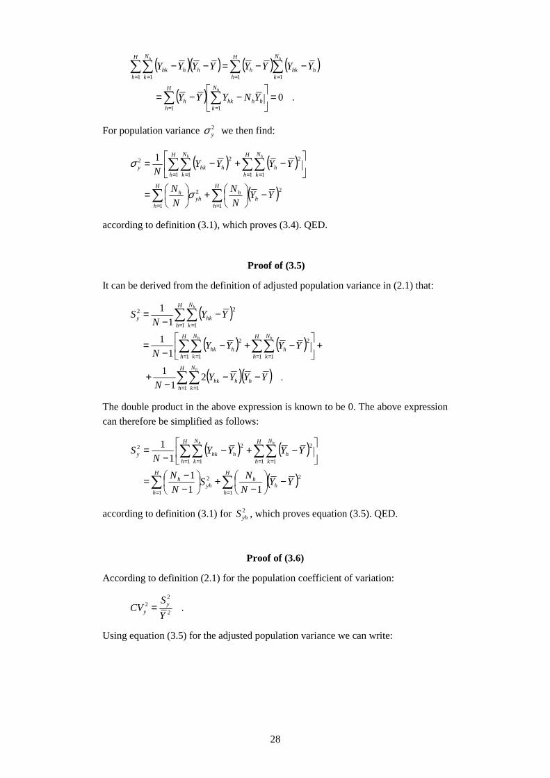
Proof of (3.5)

It can be derived from the definition of adjusted population variance in (2.1) that:

( )

( ) ( )

( )( ) .21

1

1

1

11

1 1

1 1

2

1 1

2

1 1

22

∑∑

∑∑∑∑

∑∑

= =

= == =

= =

−−−

+

+

−+−

−=

−−

=

H

h

N

khhhk

H

h

N

kh

H

h

N

khhk

H

h

N

khky

h

hh

h

YYYYN

YYYYN

YYN

S

The double product in the above expression is known to be 0. The above expression

can therefore be simplified as follows:

( ) ( )

( )∑∑

∑∑∑∑

==

= == =

−

−+

−−=

−+−

−=

H

hh

hH

hyh

h

H

h

N

kh

H

h

N

khhky

YYN

NS

N

N

YYYYN

Shh

1

2

1

2

1 1

2

1 1

22

111

11

according to definition (3.1) for 2yhS , which proves equation (3.5). QED.

Proof of (3.6)

According to definition (2.1) for the population coefficient of variation:

.2

22

Y

SCV y

y =

Using equation (3.5) for the adjusted population variance we can write:

29

( )

.111

1

11

1

1

2

1

2

2

12

2

12

22

∑∑

∑∑

==

==

−

−+

−−=

−

−+

−−=

H

h

hhH

hyh

hh

H

h

hhH

h

yhhy

Y

Y

N

NCV

Y

Y

N

N

Y

YY

N

N

Y

S

N

NCV

This proves (3.6). QED.

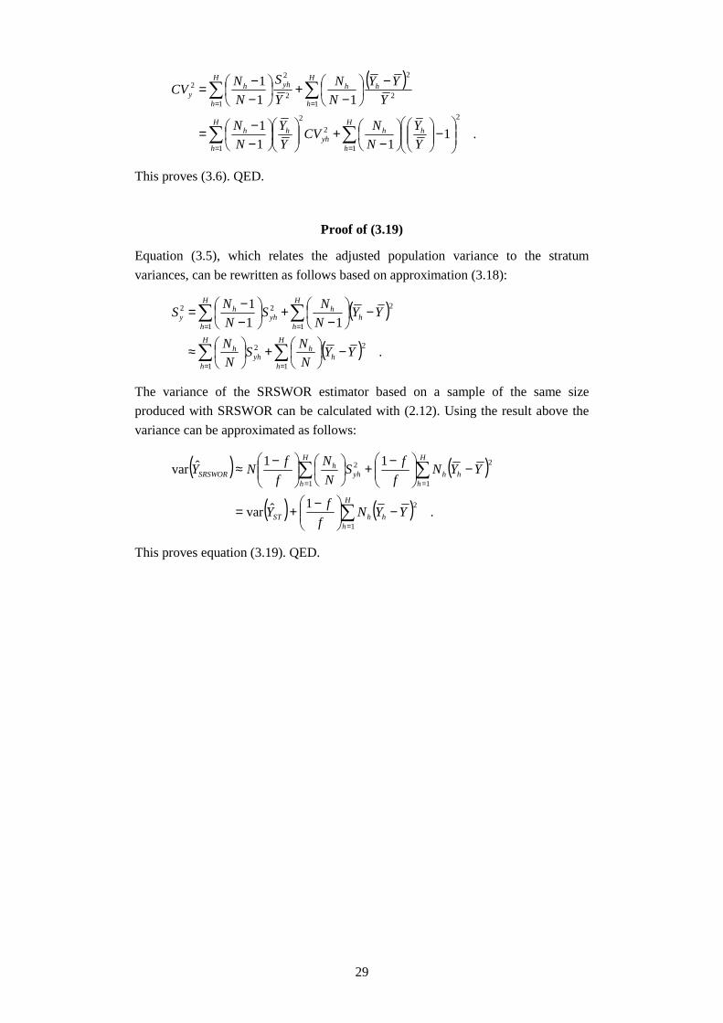
Proof of (3.19)

Equation (3.5), which relates the adjusted population variance to the stratum

variances, can be rewritten as follows based on approximation (3.18):

( )

( ) .

11

1

2

11

2

2

11

22

YYN

NS

N

N

YYN

NS

N

NS

h

H

h

hH

hyh

h

h

H

h

hH

hyh

hy

−

+

≈

−

−+

−−=

∑∑

∑∑

==

==

The variance of the SRSWOR estimator based on a sample of the same size

produced with SRSWOR can be calculated with (2.12). Using the result above the

variance can be approximated as follows:

( ) ( )

( ) ( ) .1ˆvar

11ˆvar

1

2

1

2

1

2

∑

∑∑

=

==

−

−+=

−

−+

−≈

H

hhhST

H

hhh

H

hyh

hSRSWOR

YYNf

fY

YYNf

fS

N

N

f

fNY

This proves equation (3.19). QED.

30

4. Cluster sampling, Two-stage sampling and Systematic sampling


The principle of the three types of sampling designs discussed in this chapter is a

division of the target population into clusters. The division must be such that the

clusters do not overlap and together they cover the whole population.

The clusters in a cluster sample are selected by random sampling, and then each

selected cluster is observed in full. Cluster sampling can therefore be interpreted as

random sampling of groups. In this case too we have the choice of selecting the

clusters with or without replacement.

The first stage of two-stage sampling, as in cluster sampling, involves selecting

clusters at random. Subsequently the second stage of two-stage sampling involves

taking a further random sample of elements from each selected cluster.

The systematic sampling design is also treated in this chapter because it can be

regarded as a kind of cluster sampling.

4.2 Applicability

The previous chapter introduced stratification as a sampling method in which the

population is first divided into subpopulations (the strata), and then selecting a

sample from each separate stratum. Stratified sampling generally increases the

precision of estimators. Although at first glance cluster sampling closely resembles

stratified sampling, it has very different properties. For instance, cluster sampling

usually leads to a lower precision than simple random sampling. Cluster sampling is

therefore applied only when required by the practical situation, or when the loss of

precision is compensated by a substantial reduction in the (data collection) costs.

The loss of precision arises because, unlike stratified sampling, cluster sampling

does not select all subpopulations.

Nonetheless the estimators can sometimes gain precision in a second stage by

drawing samples from the clusters that were selected in the first stage. Because the

clusters are no longer fully observed, one could consider selecting a few more

clusters in the first stage in order to create a clearer picture of the overall population.

Two-stage sampling is particularly useful with clusters that are homogeneous with

respect to the target variable.

An example of two-stage sampling is a clustering of all households in the

Netherlands according to regions or districts. A sample of households is selected in

the second stage from each district selected in the first stage. The advantage of a

regional cluster sample of this kind is the reduction in total interviewer travel

expenses compared with a random sample of all Dutch households. The travel

expenses are reduced because an interviewer can now interview a relatively large

number of individuals who live close together in clusters.

31

All sampling designs discussed so far have assumed the availability of a satisfactory

sampling frame for the target population. Clearly, this will not always be the case.

However, sampling frames may be available for subpopulations of the target

population. Suppose we want to conduct a survey of secondary school students.

There is no readily available comprehensive list of secondary school students, but

maybe we can lay our hands on a list of secondary schools without much difficulty.

Each school will obviously know the identities of its students. Other examples of

‘natural’ groups in the population include municipalities, households, businesses

and care homes. These groups then form the clusters.


This section describes three sampling designs. Firstly, we describe cluster sampling.

That is, the clusters selected in the sample are completely observed. Secondly, we

describe two-stage sampling where in the second stage subsamples are drawn from

the clusters selected in the first stage. Finally, systematic sampling is discussed

which can be seen as a special case of cluster sampling.

4.3.1 Cluster sampling

4.3.1.1 Assumptions and notation

With respect to the target variable Y we distinguish the five parameters for the

population defined in (2.1).

As with the stratified sampling design, cluster sampling subdivides the population

into subpopulations. A subpopulation is referred to as a cluster or primary sampling

unit (PSU). An implicit assumption is that the population is fully covered by the

clusters, and that the separate clusters have no common elements.

The clusters in the sampling design are initially interpreted as survey units (which is

why the clusters are not allowed to overlap in the population). A specific cluster is

identified with an index d, Nd ,,1 L= ; the number of elements in cluster d is

denoted by dM . The elements of a primary sampling unit are referred to as the

secondary sampling units (SSU). The cluster size dM is normally assumed known.

The total number of elements in the population is denoted by M. Therefore

.1

MMN

dd =∑

=

This total population size can be averaged over the number of clusters. The result is

referred to as the mean cluster size, denoted by M :

.N

MM =

The value of the target variable for element k in cluster d is denoted by dkY for

Nd ,,1 L= and dMk ,,1 L= . With respect to the target variable, the following

32

parameters are identified for each cluster: the cluster total dY , the cluster mean dY ,

the cluster variance 2ydσ , and the adjusted cluster variance 2

ydS . These parameters

are defined by:

( )

( ) .1

1

1

1

1

22

1

22

1

∑

∑

∑

=

=

=

−−

=

−=

=

=

d

d

d

M

kddk

dyd

M

kddk

dyd

dd

d

M

kdkd

YYM

S

YYM

YM

Y

YY

σ(4.1)

To these four cluster parameters can be added the mean cluster total CTY and the

adjusted variance of cluster totals 2yCTS . These are defined as follows:

( ) .1

1

11

1

22

1

∑

∑

=

=

−−

=

==

N

dCTdyCT

N

ddCT

YYN

S

YN

YN

Y

(4.2)

A simple random sample of n clusters is selected from the population of N clusters.

Each of the selected clusters is observed in full, so that for each cluster there are dm

observations with dd Mm = . It is therefore possible to interpret the random cluster

sample as a simple random sample of n out of N primary sample units with the

cluster totals as observations. The n observed cluster totals are denoted by lower

case letters .,,1 nyy L

We further define the sample mean of cluster totals CTy , and the sample variance of

cluster totals 2yCTs as:

( ) .1

1

1

1

22

1

∑

∑

=

=

−−

=

=

n

lCTdyCT

n

ddCT

yyn

s

yn

y

(4.3)

4.3.1.2 Relationships between population parameters and cluster parameters

The relationships between the population parameters and their cluster counterparts

are shown below:

.11

111

11 1

∑∑∑

∑∑∑

===

== =

====

==

N

dd

dN

ddd

N

dd

N

dd

N

d

M

kdk

YM

MYM

MY

MM

YY

YYYd

33

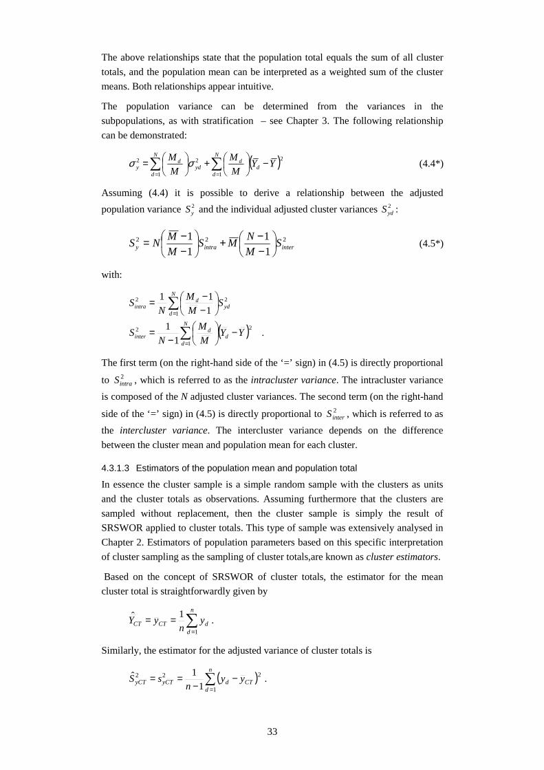
The above relationships state that the population total equals the sum of all cluster

totals, and the population mean can be interpreted as a weighted sum of the cluster

means. Both relationships appear intuitive.

The population variance can be determined from the variances in the

subpopulations, as with stratification – see Chapter 3. The following relationship

can be demonstrated:

( )∑∑==

−

+

=

N

dd

dN

dyd

dy YY

M

M

M

M

1

2

1

22 σσ (4.4*)

Assuming (4.4) it is possible to derive a relationship between the adjusted

population variance 2yS and the individual adjusted cluster variances 2

ydS :

222

11

11

interintray SM

NMS

M

MNS

−−+

−−= (4.5*)

with:

( ) .1

1

111

1

22

1

22

∑

∑

=

=

−

−=

−−=

N

dd

dinter

N

dyd

dintra

YYM

M

NS

SM

M

NS

The first term (on the right-hand side of the ‘=’ sign) in (4.5) is directly proportional

to 2intraS , which is referred to as the intracluster variance. The intracluster variance

is composed of the N adjusted cluster variances. The second term (on the right-hand

side of the ‘=’ sign) in (4.5) is directly proportional to 2interS , which is referred to as

the intercluster variance. The intercluster variance depends on the difference

between the cluster mean and population mean for each cluster.

4.3.1.3 Estimators of the population mean and population total

In essence the cluster sample is a simple random sample with the clusters as units

and the cluster totals as observations. Assuming furthermore that the clusters are

sampled without replacement, then the cluster sample is simply the result of

SRSWOR applied to cluster totals. This type of sample was extensively analysed in

Chapter 2. Estimators of population parameters based on this specific interpretation

of cluster sampling as the sampling of cluster totals,are known as cluster estimators.

Based on the concept of SRSWOR of cluster totals, the estimator for the mean

cluster total is straightforwardly given by

.1ˆ

1∑

=

==n

ddCTCT y

nyY

Similarly, the estimator for the adjusted variance of cluster totals is

( )∑=

−−

==n

dCTdyCTyCT yy

nsS

1

222 .1

1ˆ

34

There is a simple relationship between the population total Y and the mean cluster

total CTY , which can be derived from (2.1) and (4.2). There is therefore also a

similar relationship between the population mean and the mean cluster total. Both

relationships are shown below:

.1

CTCT YMM

YYYNY ==∧= (4.6)

Based on these relationships and the estimator for the mean cluster total, we arrive

at a cluster estimator for the population total Y , denoted by CLY , and a cluster

estimator for the population mean, denoted by CLY .

.111ˆ1ˆˆ

1ˆˆ

1

1

∑

∑

=

=

====

===

n

ddCTCT

CLCL

n

ddCTCTCL

yMf

yM

YMM

YY

yf

yNYNY

(4.7)

In these two formulas Nnf = represents the fraction of clusters in the random

sample. Note that the sample mean CTy of cluster totals arises naturally in these

estimators.


Because the cluster sampling procedure is SRSWOR of cluster totals, the estimator

of the mean cluster total is known to be unbiased. Based on the same argument it

can also be concluded that the sample variance of cluster totals is an unbiased

estimator of the adjusted variance of cluster totals.

By definition the cluster estimators of the population total and the population mean

are scaled versions of the estimator for the mean cluster total. This fact together with

the unbiasedness of the estimator of the mean cluster total and the dependencies

(4.6) mean that the cluster estimators of the population total and the population

mean in (4.7) are both unbiased.


We have seen that the unbiasedness of the estimator of the mean cluster total is the

basis of the unbiasedness of the two cluster estimators. Similarly, the variance

calculation for the estimator of the mean cluster total is the basis of the variance

calculations for both cluster estimators.

The variance of the estimator of the mean cluster total can be calculated as follows –

see also (2.11):

( ) .11

varˆvar 2yCTCTCT S

f

f

NyY

−==

(4.8)

35

We can infer from this result that the variance of the cluster estimator of the

population total is:

( ) ( ) 22 1ˆvarˆvar yCTCTCL Sf

fNYNY

−== (4.9)

and that for the variance of the cluster estimator of the population mean:

( ) .111ˆvar

1ˆvarˆvar 2

2 yCTCLCL

CL Sf

f

MMY

MM

YY

−

==

=

(4.10)

Estimators for results (4.8) - (4.10) can be obtained by replacing 2yCTS in the

corresponding formulas by 2yCTs . Because the sample variance of cluster totals is an

unbiased estimator of the adjusted variance of cluster totals, the estimators of the

variances (of the cluster estimators) produced in this way are unbiased.

4.3.1.4 Sampling design evaluation

To evaluate the cluster sample the design effects of the cluster estimators of the

population total and population mean have to be calculated. This involves

comparing the variance of a cluster estimator with the variance of the SRSWOR

estimator based on a sample of the same size. Unfortunately, the size of a cluster

sample is not known in advance. However, on average a cluster sample consists of

)( Mn× individual observations. The comparison with the SRSWOR estimator is

therefore also based on a sample of )( Mn× out of M elements.

The design effects of the cluster estimators for the population total and population

mean, analogous to (3.16), are defined as (assume implicitly that: 0)ˆvar( ≠SRSWORY ):

( ) ( )( )

.ˆvar

ˆvarˆ

ˆvar

ˆvarˆ

=

=

SRSWOR

CL

CL

SRSWOR

CLCL

Y

YYDEFF

Y

YYDEFF

(4.11)

Definition (4.11) formally specifies the design effects of the cluster estimators of the

population total and the population mean. However, the result given below shows

that for the remainder of this subsection it suffices to refer only to the design effect

of the cluster estimator of the population total.

[ ] ( )( )

( ) ( )( ) ( ) [ ] .ˆ

ˆvar

ˆvarˆvar

ˆvarˆ

2

2

1

1

CL

SRSWORM

CLM

SRSWOR

CLCL YDEFF

Y

Y

Y

YYDEFF ===

The variance of the SRSWOR estimator of the population total is

36

( ) 21ˆvar ySRSWOR Sf

fMY

−=

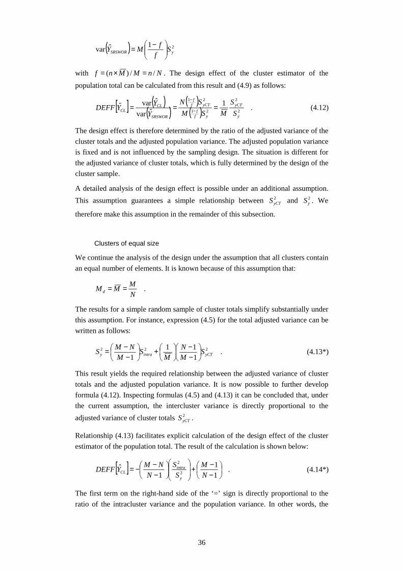
with NnMMnf //)( =×= . The design effect of the cluster estimator of the

population total can be calculated from this result and (4.9) as follows:

[ ] ( )( )

( )( ) .

1ˆvar

ˆvarˆ2

2

21

21

y

yCT

yff

yCTff

SRSWOR

CLCL S

S

MSM

SN

Y

YYDEFF === −

−

(4.12)

The design effect is therefore determined by the ratio of the adjusted variance of the

cluster totals and the adjusted population variance. The adjusted population variance

is fixed and is not influenced by the sampling design. The situation is different for

the adjusted variance of cluster totals, which is fully determined by the design of the

cluster sample.

A detailed analysis of the design effect is possible under an additional assumption.

This assumption guarantees a simple relationship between 2yCTS and 2

yS . We

therefore make this assumption in the remainder of this subsection.

Clusters of equal size

We continue the analysis of the design under the assumption that all clusters contain

an equal number of elements. It is known because of this assumption that:

.N

MMMd ==

The results for a simple random sample of cluster totals simplify substantially under

this assumption. For instance, expression (4.5) for the total adjusted variance can be

written as follows:

.111

1222yCTintray S

M

N

MS

M

NMS

−−

+

−−= (4.13*)

This result yields the required relationship between the adjusted variance of cluster

totals and the adjusted population variance. It is now possible to further develop

formula (4.12). Inspecting formulas (4.5) and (4.13) it can be concluded that, under

the current assumption, the intercluster variance is directly proportional to the

adjusted variance of cluster totals 2yCTS .

Relationship (4.13) facilitates explicit calculation of the design effect of the cluster

estimator of the population total. The result of the calculation is shown below:

[ ] .1

1

1ˆ

2

2

−−+

−−−=

N

M

S

S

N

NMYDEFF

y

intraCL (4.14*)

The first term on the right-hand side of the ‘=’ sign is directly proportional to the

ratio of the intracluster variance and the population variance. In other words, the

37

design effect (of the cluster estimator of the population total) is a decreasing linear

function of intracluster variance 2intraS .

Formula (4.14) shows an indirect relationship between the way of clustering and the

design effect of the estimator, because the intracluster variance is dependent on the

cluster design. This means that the design effect is maximal for minimum

intracluster variance and minimal for maximum intracluster variance. The range of

the design effect can therefore be determined as:

[ ] .1

1ˆ0

−−≤≤

N

MYDEFF CL (4.15*)

The lower range limit of the design effect (of the cluster estimator of the population

total) is reached if and only if the intercluster variance is zero – see also Equation

(4.5). Cluster sampling often appears less efficient in practice than SRSWOR. This

loss of efficiency therefore has to be compensated by lower costs if cluster sampling

is actually to be used.

Generally, a larger intracluster variance leads to a cluster estimator (of the

population total) with greater precision. In turn, a larger intracluster variance

corresponds with less internal homogeneity of the clusters. It is therefore advisable

to make the clusters as diverse as possible.

An alternative analysis of the design effect of the cluster estimator of the population

total uses the intraclass correlation coefficient. This alternative analysis is set out in

the remainder of this subsection..

The intraclass correlation coefficient cρ is defined as the Pearson correlation

coefficient for the )1(x −MMN paired observations ),( dldk YY within the clusters,

where lk ≠ and Nd ,,1 L= . The formal definition is:

( )( )( )( ) 2

1 1

11 y

N

d

M

k

M

kl dldkc SMM

YYYY

−−−−

=∑ ∑ ∑= = ≠ρ (4.16)

The intraclass correlation coefficient, or intracluster correlation coefficient, is a

measure of the homogeneity within the clusters. It indicates how alike or different

the elements in a cluster are. Maximum homogeneity of the clusters corresponds

with 1=cρ . Mutatis mutandis, minimum cluster homogeneity corresponds with

maximum intracluster variance.

Closer examination reveals the possibility of expressing the intracluster correlation

coefficient in terms of the ratio of the adjusted variance of cluster totals and the

adjusted population variance, i.e.:

( )( ) .1

1

11

12

2

−−

−−

−=MS

S

MM

N

y

yCTcρ (4.17*)

This result shows that the intracluster correlation coefficient is a linearly increasing

function in the adjusted variance of cluster totals 2yCTS . In other words, cρ is an

38

increasing function in the intercluster variance 2interS , because the latter is a multiple

of 2yCTS . To conclude, the coefficient cρ is minimal for the smallest possible

intercluster variance and is maximal for the greatest possible intercluster variance.

The range of the intracluster correlation coefficient can thus be determined directly

and equals:

.11

1 ≤≤

−− cM

ρ (4.18*)

Finally, equation (4.16) allows the design effect of the cluster estimator of the

population total to be written as a function of cρ . Analysis shows that for 1>>N :

[ ] ( ){ }( ){ } .11

111ˆ

c

cCL

M

MMM

MYDEFF

ρ

ρ

−+≈

−+−−=

(4.19*)

The design effect is therefore a linear function of cρ ; the approximation in (4.19)

holds when the number of clusters N is large. The linearly increasing nature of the

relationship means that the design effect reaches a minimum value for the smallest

possible intracluster correlation coefficient. Mutatis mutandis, the maximum design

effect is obtained for the greatest possible intracluster correlation coefficient. The

intraclass correlation coefficients is usually positive in practice. In particular when

the clusters form ‘natural’ groups in the population, the elements within a cluster

will resemble each other more than elements selected at random from the

population. This resemblance may be attributable to coming from a common

background or environment. When the elements within a cluster are similar to each

other, the intracluster variance 2intraS will be relatively small compared with the

adjusted population variance 2yS , so that cρ will be positive. In addition, cρ will be

negative only if the elements in a cluster exhibit a greater variance than a randomly

selected group of elements. This will seldom be the case, but may occur with

artificially formed clusters in which elements are allocated randomly to clusters.

4.3.2 Two-stage sampling

The cluster sample discussed above always involved investigating all elements of

every selected cluster. It was shown that cluster sampling is not very efficient when

the clusters are fairly homogeneous. If the elements within a cluster very closely

resemble each other, it may actually be a waste of time and money to investigate all

elements; the same information could have been obtained by examining just a

couple of elements. In such cases cluster sampling will perform fairly poorly, and it

may be worthwhile to take a sample from the selected clusters. This is referred to as

two-stage sampling.

The first stage of two-stage sampling involves selecting clusters or primary

sampling units at random. The second stage of two-stage sampling involves

randomly selecting elements, which are now referred to as secondary sampling

units, from each selected primary sampling unit.

39

Assuming that the clusters are homogeneous, two-stage sampling generally allows

more clusters to be selected in the first sampling stage, which may increase

precision. This method gives greater control of sample size where the sizes of

primary sample units vary greatly. Note that, in this case too, a sampling frame is

required only for the selected primary sample units.

The costs and precision of two-stage sampling fall roughly between those of cluster

sampling and stratified sampling. Two-stage sampling is generally more expensive

than cluster sampling with the same sample size, but less expensive than stratified

sampling. On the other hand, two-stage sampling is generally more precise than

cluster sampling and less precise than stratified sampling.

It is easy to extend two-stage sampling to multistage sampling (with three, four, or

more stages). For example, selecting a sample of secondary school students could

involve selecting a sample of schools, then selecting a number of classes within a

selected school, and finally selecting a number of students within a selected class.

Another example is sampling successively by region, city, postcode area, and

address. The units in the final stage are the sample elements. Here, the discussion is

confined to two-stage sampling, because of its simplicity, but also because it is a

more common design in practice than multistage sampling.

The design of two-stage sampling involves determining the selection methods for

both the primary and secondary sampling units. The two methods do not have to be

the same. It is possible to select units in various ways at each stage: random, or

systematic, or proportional to size (see Sections 4.3.3 and 5.1.2 for details). The

units may also be stratified first.

Apart from the selection methods in the two stages, it is also necessary to decide on

the distribution of the sample over the first and the second stages. Is it better to

select a relatively large number of primary sampling units and few secondary

sampling units, or relatively few primary sampling units and many secondary

sampling units? The first case will generally yield more precise estimators, but often

at greater expense.

4.3.2.1 Assumptions and notation

The current analysis assumes SRSWOR in both stages. The notation used is almost

analogous to that for the cluster sampling design. The population is again divided

into N nonoverlapping clusters, or primary sampling units. In the first stage n

primary sampling units are selected. Then in the second stage, dm secondary

sampling units are selected from each primary sampling unit, where in general

dd Mm ≠ . Sample size dm , nd ,,1 L= is assumed to be determined in advance. The

measured value of the target variable for element k in selected cluster d is denoted

by ,dky .,...,1 dmk = Furthermore, define for each (sub)sample the two quantities

sdy and 2yds as:

40

( ) .1

1

1

1

22

1

∑

∑

=

=

−−

=

=

d

d

m

ksddk

dyd

m

kdk

dsd

yym

s

ym

y

(4.20)

4.3.2.2 Estimators in two-stage sampling

Two-stage sampling does not involve observing all secondary sampling units in the

selected primary sampling units. The cluster parameters of the (selected) primary

sampling units therefore have to be estimated. The cluster total dy in primary

sampling unit d can be estimated by:

( ) .,,1ˆ1

ndym

MyMy

dm

kdk

d

dsddd L=== ∑

=

(4.21)

In other words, the estimated cluster total corresponds with a weighted sum of the

observed secondary sampling units (in the primary sampling unit referred to

previously). The weighting factor is the reciprocal of the sampling fraction for

primary sampling unit d.

The population mean CTY of cluster totals can be estimated by:

.ˆ1

ˆˆ

1∑

=

==n

ddCTCT y

nyY

Consequently, the cluster estimators of the population total and population mean are

.ˆˆ1ˆ

ˆˆˆ

12

12

∑

∑

=

=

==

==

n

ddCTCL

n

ddCTCL

ynM

NY

MY

yn

NYNY


The fact that a selected cluster (primary sampling unit) is no longer observed in full,

but through an SRSWOR sample of dm out of dM , has no influence on the analysis

of bias for the estimators. That is, all estimators defined so far in this subsection are

unbiased.


The variances of the estimators CLY and CLY in conventional cluster sampling are

determined only by the differences between the clusters. However, the estimated

cluster totals dy in two-stage sampling are stochastic variables. Consequently, the

variation within the clusters also contributes to the variance of the estimators. The

variance of the cluster estimator of the population total 2CLY therefore comprises an

additional term :

41

( ) .11ˆvar

1

2

,21

,22

1

12 ∑

=

−+

−=N

dyd

d

ddyCTCL S

ff

fMS

f

fNY (4.22*)

with:

.,21d

dd M

mf

N

nf =∧=

The first fraction is referred to as the first-stage sampling fraction; the second

fraction is referred to as the second-stage sampling fraction.

The variance of the cluster estimator of the population mean is obtained by dividing

the variance of the cluster estimator of the population total by 2M :

( )

.11111

ˆvar1ˆvar

1

2

,21

,22

1

1

222

∑=

−

+

−

=

=

N

dyd

d

ddyCT

CLCL

Sff

f

M

M

MS

f

f

MM

YM

Y

The effect of sampling in the second stage on the variance above is clear from a

comparison of (4.22) with (4.9). The variances of the estimators comprise two

terms. The first term (on the right-hand side of the ‘=’ sign) is attributable to the

differences between the totals of the primary sampling units. The second term (on

the right-hand side of the ‘=’ sign) is attributable to the variation within the primary

sampling units. This term played no part in the above sections because the clusters

were observed in full ( 1,2 ≡df ). In many situations the second term will be

negligible relative to the first term. With a strongly varying dM , an objection to the

SRSWOR estimator in the first stage is that the cluster totals usually differ very

substantially. This effect can be countered by selecting the primary sampling units

in proportion to their size, or by employing the ratio estimator.

The calculated variance (4.22) can be estimated without bias by

( )

( ) .ˆˆ1

1

11ˆrav

1

22ˆ

1

2

,21

,22ˆ

1

12

∑

∑

=

=

−−

=

−+

−=

n

dCTdCTy

n

dyd

d

ddCTyCL

yyn

s

sff

fMs

f

fNY

(4.23*)

Sampling design evaluation

In two-stage sampling on average )( mn× secondary sampling units are

interviewed; the expected mean of the sample sizes in the n chosen primary units is

∑ == N

d d Nmm1

)/( . To evaluate this cluster sample we compare the variance of the

cluster estimators with the variance of the corresponding estimators based on

SRSWOR of )( mn× out of M elements. To this end, the design effect of the

cluster estimator of the population total is calculated – see Definition (4.11).

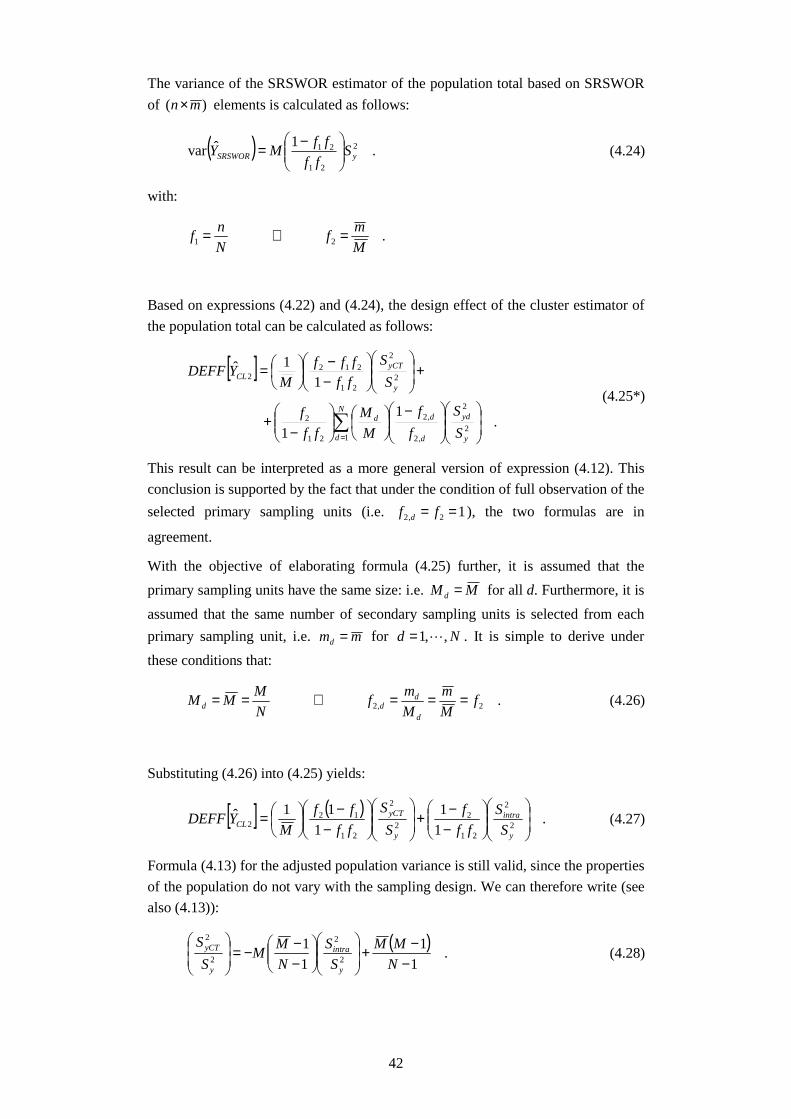
42

The variance of the SRSWOR estimator of the population total based on SRSWOR

of )( mn× elements is calculated as follows:

( ) .1ˆvar 2

21

21ySRSWOR S

ff

ffMY

−= (4.24)

with:

.21 M

mf

N

nf =∧=

Based on expressions (4.22) and (4.24), the design effect of the cluster estimator of

the population total can be calculated as follows:

[ ]

.1

1

11ˆ

12

2

,2

,2

21

2

2

2

21

2122

∑=

−

−

+

+

−−

=

N

d y

yd

d

dd

y

yCTCL

S

S

f

f

M

M

ff

f

S

S

ff

fff

MYDEFF

(4.25*)

This result can be interpreted as a more general version of expression (4.12). This

conclusion is supported by the fact that under the condition of full observation of the

selected primary sampling units (i.e. 12,2 == ff d ), the two formulas are in

agreement.

With the objective of elaborating formula (4.25) further, it is assumed that the

primary sampling units have the same size: i.e. MMd = for all d. Furthermore, it is

assumed that the same number of secondary sampling units is selected from each

primary sampling unit, i.e. mmd = for Nd ,,1 L= . It is simple to derive under

these conditions that:

.2,2 fM

m

M

mf

N

MMM

d

ddd ===∧== (4.26)

Substituting (4.26) into (4.25) yields:

[ ] ( ).

1

1

1

11ˆ2

2

21

22

2

21

122

−−+

−

−

=

y

intra

y

yCTCL S

S

ff

f

S

S

ff

ff

MYDEFF (4.27)

Formula (4.13) for the adjusted population variance is still valid, since the properties

of the population do not vary with the sampling design. We can therefore write (see

also (4.13)):

( ).

1

1

1

12

2

2

2

−−+

−−−=

N

MM

S

S

N

MM

S

S

y

intra

y

yCT (4.28)

43

This result yields the desired connection between the adjusted variance of cluster

totals and the adjusted population variance. For two-stage sampling the design effect

of the cluster estimator of the population total can also be determined after

substituting (4.28) in (4.27), as follows:

[ ]

.1

1

1

11

11

1

1ˆ

21

212

2

2

21221

2

−−

−−+

+

−−+

−−−

−

=

N

M

ff

fff

S

Sff

N

NMf

N

M

ffYDEFF

y

intraCL

(4.29)

As expected, this expression corresponds with formula (4.14) under the condition of

fully observing the selected primary sampling units (i.e. 12 =f )

4.3.2.3 Determination of sample size

As with a simple random sample, the total sample size can be determined from the

precision that is required for an estimator. Once the total sample size has been

determined, the question arises as to how to distribute it among the primary and

secondary sampling units. In other words, how many secondary sampling units

should be selected from the selected primary sample units, and how many primary

sample units should be in the sample. These questions usually involve balancing

costs and precision. Selecting many primary sampling units with few secondary

sampling units per primary unit will generally lead to small variances. However, the

potential costs saved by observing a large number of elements within one primary

sampling unit are then almost totally lost. While it is less expensive to observe many

secondary sampling units within a limited number of primary sampling units, it will

lead to less precise estimators. Answering the question about how to distribute the

sample requires some knowledge of the data collection and other costs in both

stages, and of the homogeneity of the primary sample units.

With perfectly homogeneous primary sampling units, i.e. 02 =intraS , one might as

well select just one element per primary sampling unit; observing more elements

would lead only to higher costs with no gain in precision. In all other cases the

distribution of the sample will depend on the costs of selecting the units in the two

stages. A simple cost function is:

21 cmnncC +=

where parameters 1c and 2c correspond, for example, to interview and/or travel

expenses in the first and second sampling stage. Given this cost function and fixed

total cost C, the variance of the cluster estimator of the population total is minimized

by selecting:

mcc

Cn

21 +=

primary sampling units in the sample and:

44

( ) ( )MSS

cc

c

c

SSM

SMm

intrainterintrainter

intra

/1/

/22

21

2

122

2

−=

−=

secondary sampling units per primary sampling unit. To determine these quantities

explicitly requires some idea of the ratio 22 / intrainter SS , or in other words of the

homogeneity of the primary sampling units. In practice one will often proceed the

other way around. This usually means trying different values of n and m, calculating

the associated variance of an estimator, and assessing whether this might be

acceptable.

4.3.3 Systematic sampling

Systematic sampling is frequently put forward as a good alternative to SRSWOR. In

a systematic sample of n elements out of a population of N elements, first a step

length nNL /= is determined. We assume for convenience that the elements are

numbered from 1 through N. A starting number R is then chosen at random from the

interval (0, L). The first element selected in the sample is the one with number 1k

for which .1 11 kRk ≤<− The second element selected in the sample has number 2k ,

for which ,1 22 kLRk ≤+<− and so on. The final nth element in the sample has

number nk , for which .)1(1 nn kLnRk ≤−+<− In other words, the elements with

numbers nkk ,,1 L form the sample, or the numbers in the sample are equal to the

(rounded) numbers LnRLRLRR )1(,,2,, −+++ L . It is clear that the randomly

selected starting number R determines the entire sample, and that every element

from the population can occur in only a single sample.

In theory, and assuming that L is a whole number, different samples are possible for

a fixed population sequence L, so that the sampling probability for systematic

sampling is:

( ) .1

N

n

LsP ==

Since each element can occur in only one sample, the inclusion probability of

population element k is equal to the sampling probability, i.e.:

.1

N

n

Lk ==π

With this form of systematic sampling the number of possible samples is less than

for SRSWOR with the same sample size, as not every combination of n elements is

possible. However (see the result above), the first-order inclusion probabilities are

the same as with SRSWOR. Although the systematic sample described here in fact

constitutes a cluster sample, the variance of the estimator is often approximated in

practice by that of the SRSWOR estimator. The assumption is that the (fixed)

sequence of the population elements does not lead to a systematic difference with

the SRSWOR estimator.

45

Estimators, unbiasedness and variance calculations

Systematic sampling thus amounts to selecting one cluster of size n out of L clusters.

The population parameters are estimated from the sample statistics of this single

selected cluster. The respective cluster estimators for the population total and

population mean are:

.ˆˆ yYyNY syssys =∧=

The bias of the estimators follows from the properties of cluster sampling. The

variance for the cluster estimator of the population mean for a sample of 1 cluster is

according to formula (4.10):

2

21

1ˆvarn

S

LY yCT

sys

−=

(4.30)

The variance is expressed in the notation for systematic sampling. Note that N and n

refer here to elements rather than clusters. The size of a cluster (systematic

sampling) is now n; the total number of elements is N; the number of clusters is L.

The variance of the cluster estimator for the population total is obtained by

multiplying the variance of the cluster estimator for the population mean by 2N .

Sampling design evaluation

Finally, the design effect of the cluster estimator for the population can be calculated

using formula (4.19) as:

( ){ } .111ˆ

csys nnN

NYDEFF ρ−+

−−=

Systematic sampling is therefore better than simple random sampling if and only if

the intraclass correlation coefficient satisfies:

.1

11

1−

−≤≤−

−Nn cρ

When the variance within the possible systematic samples is greater than the

population variance, the cluster means will differ little from each other, and

systematic sampling will be more precise than simple random sampling. Otherwise,

if the variance within the systematic samples is small relative to the population

variance )0( cρ< then all elements in the sample will give the same kind of

information and the variance of the estimator for systematic sampling will be larger

than for simple random sampling.

However, a significant drawback of a systematic sampling design is the lack of

unbiased estimators for the different variances. Since only one cluster is selected,

the sample variance of the cluster totals 2yCTs is undefined. Nonetheless, the variance

can be approximated if we know something about the structure of the population.

The following three situations can be identified:

46

1. random sequences of the sampling frame;

2. positive autocorrelation;

3. periodic fluctuations.

Note to 1 (random sequences of the sampling frame)In many situations it can be assumed that the values of the target variables do not

correspond with the sequence in the sampling frame. An example would be a frame

in which people are in alphabetical order. In this case systematic sampling will

correspond closely to simple random sampling )]1/(1[ c −−≈ Nρ and both samples

will produce the same sort of results. We can therefore use the variance formula for

simple random sampling to estimate )ˆvar( sysY .

Note to 2 (positive autocorrelation)Sometimes a frame will have an increasing or decreasing sequence effect. For

example, companies may appear in order of decreasing size in a list. In these cases

positive autocorrelation is said to exist: successive elements resemble each other

more closely than elements that are further apart. Systematic sampling would ensure

more spread in the sample elements and will therefore be more precise than simple

random sampling )].1/(1)1/(1[ −−<≤−− Nn cρ The variance formula for simple

random sampling would give an overestimate in this case.

Note to 3 (periodic fluctuations)Problems may occur if the sampling frame exhibits a periodic variation with respect

to a target variable. Systematic sampling will then be considerably less precise than

simple random sampling, in particular when the step length is the same as, or a

multiple of, the period. The variance of the estimator will then be extremely large,

which is not apparent when using the simple random variance formula to estimate

the variance.

Suppose the population elements are arranged so that the target variable shows the

following pattern: LL,5,4,3,2,1,5,4,3,2,1,5,4,3,2,1 . With a step length of 5 the

elements that appear in the sample will all be the same and the variance formula for

simple sampling will estimate the variance as 0)ˆr(av =Y . However, the actual value

of )ˆvar( sysY for this population is 22 =yσ ; note that .1=cρ In other words, a

systematic sample in this case is as efficient as an SRSWOR sample of size .1=n


An important quality indicator for (multistage) cluster sampling is the cost reduction

that results from the clustering of the units to be observed. The price to be paid for

this clustering in the form of increased variance relative to simple random sampling

without replacement is another important criterion.

47

4.5 Appendix

Proof of (4.4)

From the definition of population variance we can deduce:

( )

( ) ( )∑∑∑∑

∑∑

= == =

= =

−+−=

−=

N

d

M

kd

N

d

M

kddk

N

d

M

kdky

dd

d

YYM

YYM

YYM

1 1

2

1 1

2

1 1

22

11

1σ

because the double product is zero – see also the proof of (3.4). Further elaboration

of this expression gives the following result:

( )

( ) .

1

1

2

1

2

1 1

2

1

22

∑∑

∑∑∑

==

= ==

−

+

=

−+

=

N

dd

dN

dyd

d

N

d

M

kd

N

dyd

dy

YYM

M

M

M

YYMM

M d

σ

σσ

QED.

Proof of (4.5)

It can be deduced from definitions (2.1) and (4.1) that:

.11

2222yd

d

dydyy M

MS

M

MS σσ

−

=∧

−=

Multiplying equation (4.4) by the factor ))1(( −MM gives the following

relationship:

( )∑∑==

−

−+

−

=

−

N

dd

dN

dyd

dy YY

M

M

M

M

M

M

M

M

M

M

1

2

1

22 .111

σσ

This equation can be rewritten as:

( )

( )

( ) .11

1

111

1

11

1

2

1

2

1

2

1

2

1

2

1

22

∑∑

∑∑

∑∑

==

==

==

−

−+

−−=

−

−+

−−

−=

−

−+

−=

N

dd

dN

dyd

d

N

dd

dN

dyd

d

dd

N

dd

dN

dyd

dy

YYM

MS

M

M

YYM

M

M

M

M

M

YYM

M

M

MS

σ

σ

QED.

Proof of (4.13)

The proof of (4.13) starts from formula (4.5) for adjusted population variance. The

following relationships are also significant:

48

.11

ddCT YM

YYM

Y =∧=

The expression for adjusted population variance can be rewritten as:

( )

( )

( ) ( )

.1

11

1

1

1

1

1

1

1

1

11

1

11

1

22

1

2

1

2

1

22

1

2

1

2

1

22

yCTintra

N

dCTd

N

dyd

N

dCTd

N

dyd

N

dd

dN

dyd

dy

SM

N

MS

M

NM

YYN

N

MMS

N

N

M

M

YYMM

MS

M

M

YYM

MS

M

MS

−−

+

−−=

−

−−

−

+

−−=

−

−

+

−−=

−

−+

−−=

∑∑

∑∑

∑∑

==

==

==

QED.

Proof of (4.14)

Formula (4.13) for the population variance can be rewritten as follows:

222

1111

intrayyCT SM

NMSS

M

N

M

−−−=

−−

from which:

.11

11 222intrayyCT S

N

NMS

N

MS

M

−−−

−−=

Substituting this relationship into formula (4.12) gives:

[ ]

.11

1

ˆ

2

2

2

21

y

intra

y

yCTMCL

S

S

N

NM

N

M

S

SYDEFF

−−−

−−=

=

QED.

Proof of (4.15)

The design effect of the cluster estimator of the population total is minimal when the

intracluster variance is maximal. According to (4.5), the intracluster variance

obtains its maximum value if and only if the intercluster variance is zero. The value

of 2intraS can therefore be determined as follows:

.1 2

0

22 ySintra S

NM

MS

inter

−−=

=

The design effect for this value of intracluster variance is:

49

[ ] .0111

1ˆ

02=

−−+

−−

−−−=

= N

M

NM

M

N

NMYDEFF

interSCL

The design effect of the cluster estimator of the population total is maximal if the

intracluster variance is minimal. The minimum value that the intracluster variance

can assume is 0. The maximum value that the design effect can assume is then

simply:

[ ] .11ˆ

02 −−=

= N

MYDEFF

intraSCL

QED.

Proof of (4.17)

Algebraic manipulation shows that:

( )( ) ( ) ( )

( ) .2

1 11 1

CTd

M

k

M

ldldk

M

k

M

ldldk

YY

YYYYYYYY

−=

−−=−− ∑ ∑∑∑= == =

It can then be deduced from this result and definition (4.2) that:

( )( ) ( )( ) .1 2

1

2

1 1 1

yCT

N

dCTd

N

d

M

k

M

ldldk

SN

YYYYYY

−=

−=−− ∑∑∑∑== = =

There is an alternative approach to calculating the above threefold sum, as follows:

( )( ) ( )( )

( )

( )( ) ( ) .1 2

1 1

1 1

2

1 11 1 1

y

N

d

M

k

M

kldldk

N

d

M

kdk

N

d

M

k

M

kldldk

N

d

M

k

M

ldldk

SMYYYY

YY

YYYYYYYY

−+−−=

−+

−−=−−

∑∑∑

∑∑

∑∑∑∑∑∑

= = ≠

= =

= = ≠= = =

Combining these two results gives the following expression:

( )( ) ( ) ( ) .11 22

1 1yyCT

N

d

M

k

M

kldldk SMSNYYYY −−−=−−∑∑∑

= = ≠

It can be concluded from definition (4.16) for the intracluster correlation coefficient

and this result that:

( ) ( )( )( )

( )( ) .1

111

1

11

11

2

2

2

22

−−

−−

−=

−−−−−

=

MS

S

MM

N

SMM

SMSN

y

yCT

y

yyCTcρ

QED .

50

Proof of (4.18)

The intercluster variance is maximal if and only if the intracluster variance is 0. It

follows from equation (4.13) that under this condition the adjusted variance of

cluster totals is:

( ).

1

1 2

0

22 ySyCT S

N

MMS

intra

−

−==

Substituting this result into (4.17) gives:

( )( )( )

.11

11

11

11

111

02

=−

−−

=

−−

−

−

−−

−==

MM

M

MN

MM

MM

NintraScρ

The minimum value of the intercluster variance is 0. This means that the minimum

value of the adjusted variance of cluster totals is likewise 0. From the above:

.1

102 −

−== MinterScρ

QED.

Proof of (4.19)

It can be deduced from formula (4.17) that:

( )( ).

11

111

2

2

−−+

−

−−=N

M

N

MM

S

Sc

y

yCT ρ

Substituting this result in expression (4.12) for the design effect of the cluster

estimator of the population total gives:

[ ] ( )( )

( )( ).

111

1

11

1

111ˆ

MM

M

MM

MM

N

M

MN

MM

MYDEFF

c

cCL

−−+

−

−−=

−−×+

−

−−=

ρ

ρ

QED.

Proof of (4.22)

The proofs of (4.22) and (4.23) are taken from Knottnerus (2011b). Denoting the

variance of dY by 2dσ ),,,1( Nd L= it is seen from Chapter 2 that for SRSWOR

sampling in the second stage,

2

,2

,22 1)ˆvar( yd

d

dddd S

f

fMY

−==σ .

51

Recall that an SRS sample of n clusters in the first stage can simply be obtained by

taking the first n clusters after the N clusters are put in a random order. Denote the n

observed clusters in the first-stage sample s by .,..., .1 ndd Recall that kd (k =1,…,n)

can be regarded as a random variable with NddP k /1)( == ).,...,1( Nd = In order

to avoid double subscripts, the quantities kdY and

kdY of the clusters selected in s

are in the remainder briefly denoted by the lower case letters ky and ,ky

respectively ).,...,1( nk = Define the corresponding sampling errors kg by

.ˆ kkk yyg −= Define 2gCTσ by ./)( 2

12 Nd

NdgCT σσ =Σ= Then using ,0)( =kgE it is seen

that

( ) ( ){ }( )

.0)(1

)}({),cov(

11

)var(

1

2

1

2

1

2

22

====

====

==

∑

∑∑

=

==N

dkkdkkkkk

gCT

N

dd

N

dkk

kkkk

ddgEYN

dygEEyg

NddgE

N

dgEEgEg

σσ

In the same way it can be shown that kg is uncorrelated with ly and lg ).( kl ≠

Denote the sample mean of ngg ,,1 L by .CTg Now using ,ˆ CTCTCT gyy += it is

seen that

( ) ( ) ( )

.1

)var(1

varvarvar)ˆvar(

1

22

1

1

12

22

1

1

222

f

NS

f

fN

gn

NS

f

fN

gNyNgyNyN

gCTyCT

n

kkyCT

CTCTCTCTCT

σ+

−=

+

−=

+=+=

∑=

QED.

Proof of (4.23)

Similar to 2ˆCTys , denote the sample variances of the ky and kg by 2

yCTs and ,2gCTs

and their sample covariance by .ygCTs The key feature in two-stage sampling is that

ngg ,,1 L are mutually uncorrelated random variables with zero expectation and

variance .2gCTσ Therefore, ;)( 22

gCTgCTsE σ= the proof runs along the same lines as in

the well-known (hypothetical) case that ngg ,,1 L are independent and identically

distributed random variables with zero expectation and variance ;2gCTσ see also

Särndal et al. (1992, p. 52). Furthermore, 22 )( yCTyCT SsE = ; see Chapter 2. As we

have seen, kg (k=1,…,n) is uncorrelated with .,,1 nyy L Hence,

.)2()()( 22222,

2ˆ gCTyCTygCTgCTyCTCTgyCTy SsssEsEsE σ+=++== + (4.31)

In addition, define 2ˆdσ by

52

2

,2

,22 1ˆ yd

d

ddd s

f

fM

-=s .

It follows from Chapter 2 that 2ˆds is an unbiased estimator of .2ds Furthermore, in

analogy with NYnyEyE kskCT /)/ˆ()ˆ( =S= Î ,

.1ˆ1 2

1

2

1

2gCT

N

dd

n

kk Nn

E sss ==

∑∑==

(4.32)

Using (4.31) and (4.32), it is seen that ( )2ˆrav CLY in (4.23) is unbiased. QED.

Proof of (4.25)

The design effect of the cluster estimator of the population total is defined as the

ratio between variances (4.22) and (4.24). It can therefore simply be deduced that:

[ ]

( )

.1

1

1

11

1

1

1

1

11ˆ

12

2

,2

,2

21

2

2

2

21

12

12

2

,21

,2

21

21

2

2

21

21

1

12

∑

∑

=

=

-

-

+

+

-

-

=

-

-

+

-

-=

N

d y

yd

d

dd

y

yCT

N

d y

yd

d

dd

y

yCTCL

S

S

f

f

M

M

ff

f

S

S

ff

ff

M

S

S

ff

fM

ff

ff

M

S

S

ff

ff

Mf

fNYDEFF

QED.

53

5. Samples with equal and unequal inclusion probabilities


5.1.1 The advantage

When drawing a sample not all the elements in a population need to be given the

same inclusion probability, as has been done so far. Especially when the target

variable kY in the population is roughly proportional to a particular auxiliary

variable ),,1( NkX k L= , sampling with unequal inclusion probabilities is

preferable. The latter variable must then be known for all elements in the

population. In practice the auxiliary variable kX often stands for the size or the

relevance of element k in the entire population.

There are many ways of sampling without replacement with unequal inclusion

probabilities. This chapter focuses on systematic ‘probability proportional to size’

(PPS) samples, where the elements are in random order and the inclusion

probabilities are proportional to a given auxiliary variable kX – see the example in

section 5.4. The great advantage of unequal inclusion probabilities is that the

variances of the estimators can be reduced substantially, thereby also reducing the

corresponding margins of uncertainty. Another advantage is that stratification in size

classes is no longer necessary, so avoiding for a given sample size the risk of having

extremely few observations in some strata.

5.1.2 The sampling scheme for systematic PPS sampling

After randomly ordering the population elements, every element k is assigned an

interval with length kX (on the real line) Nk ,,1 L= . The first element is assigned

the interval ],0( 1X by definition, the second element the interval ],,( 211 XXX + and

so on. As a result, the interval ],0( X , where X stands for the population total of the

auxiliary variable, is divided into N consecutive intervals. Subsequently, ],0( X is

divided into n equal pieces of length L )/( nXL = ; L is also referred to as the step

length.

The sampling scheme is now as follows. Randomly select a number r between 0

and L . This number falls in exactly one of the intervals that comprise ],0( X . The

population element that corresponds with this interval is the first element selected in

the sample. The population element the assigned interval of which contains the

number )( Lr + becomes the 2nd element in the sample, and so on. The final element

in the sample is the one where the assigned interval comprises the number

])1([ Lnr −+ . This sampling scheme can be represented in formulas as follows:

54

.)(0for )(

0

),,1(

1

0

1

XxSxSkxJ

S

NkXXS

kk

kk

≤<≤<==

=++=

−

LL

The systematic PPS sample then consists of the n elements with ranks

))1((,),(),( LnrJLrJrJ −++ LL

To avoid multiple inclusion of an element in the sample, we have tacitly assumed

that elements for which kXL < have already been removed from the population and

included in a separate stratum, which is observed in full. This stratum is said to

contain the self-selecting elements. Having removed the self-selecting elements, X

must be recalculated, just as the new L and the new sample size n. If necessary, this

process must be repeated until no new self-selecting elements appear.

The elements in the sampling scheme described here are first randomly ordered.

However, sometimes there may be a good reason for maintaining some fixed

sequence of elements, e.g. a sequence of increasing kX . If kk XY / and kX are

closely related, this kind of sequence can produce estimators with a particularly

small variance. Nonetheless, identifying a good variance estimator can be a

problem. Standard variance estimators do not exist, but under certain modelling

assumptions reasonably reliable variance estimators can be derived.

Note that it is unnecessary to randomly order the elements when there is no

substantial relation between kk XY / and kX , or, more precisely, when there is no

relation between kk XY / and k , Nk ,,1L= . In these situations random sequencing

of the elements will have no systematic effect on the outcomes.

Finally, we mention the special case of all elements having the same inclusion

probability, which is to say that all elements are assigned an interval of the same

length, while the kX differ. With elements that are randomly arranged, this

approach is equivalent to SRSWOR, in which case the formulas given in Chapter 2

apply. If, conversely, the elements are in a fixed sequence, it is again much more

difficult to estimate the variance of the estimator of the population total. However, it

is possible to demonstrate that the variance decreases if the elements are arranged

such that all possible samples resemble each other (and therefore also the

population) as closely as possible in terms of the distribution of the kX . This

situation can be approached in practice by ordering the elements according to size of

the .kX A condition for reducing the variance of the estimator of the population

total is that a sufficiently high correlation exists between kY and .kX

Another option is to arrange the elements as much as possible according to region,

so that every sample has sufficient regional spread (heterogeneity). In other words,

the (fixed) sequence must prevent the samples thus selected becoming

homogeneous. As with unequal inclusion probabilities, a remaining problem is

tracing the variance – see Knottnerus (2003, pp 190-1 and 237-43).

55

5.2 Applicability

Statistics Netherlands applies the PPS sampling design mainly in social statistics,

such as in the two-stage sampling of individuals. In the first stage, municipalities are

selected with an inclusion probability proportional to the number of residents. In the

second step individuals are selected by means of SRSWOR from each municipality

selected in the first stage. The second-stage sampling fraction in turn is inversely

proportional to the number of residents of the corresponding municipality, so that on

balance all individuals have the same inclusion probability.

Following the example of other countries, Statistics Netherlands will shortly also be

using the PPS sampling design for estimating the monthly producer price index

(PPI) for industry. In a specific example using data from 2005, the theory for the

PPI is worked out in Section 5.4.



The starting point is a population of N elements from which a sample of size n is to

be selected without replacement, unless stated otherwise. It is assumed in this

chapter that the sample size n is fixed. As in the previous chapters, we are interested

in estimating the population mean Y and the population total Y . The n sample

observations of the target variable are denoted with nyy ,,1 L .

The binary selection indicator ka – see (2.7) – is a random variable that states

whether or not element k from the population was ultimately included in the

sample.

The probability of population element k being selected in the sample, i.e. the

inclusion probability, is denoted with the symbol kπ . The formal definition of the

inclusion probability is:

NkaP kk ,,1)1( L===π (5.1)

with:

=sample.in theincludedelement if0

samplein theincludedelement if1

notisk

iskak

The second-order inclusion probability for the two population elements k and l ,

denoted as klπ , is the probability of population elements k and l occurring together

in the sample. Expressed more formally this is:

( )

===≠=∧=

=.,,1

,,111

Nlk

NlkaaP

k

lkkl

L

L

ππ (5.2)

56

5.3.2 Estimators for the population total and the population mean

Given the (unequal) inclusion probabilities kπ for all N elements of the population,

the population total Y can be estimated with the Horvitz-Thompson (HT) estimator.

The HT estimator, denoted as HTY , is defined as:

.ˆ1∑

=

=n

k k

kHT

yY

π(5.3)

A necessary condition for applying this estimator is that the inclusion probability kπis greater than 0 for .,,1 Nk L= Definition (5.3) leads immediately to the definition

of the Horvitz-Thompson estimator of the population mean, denoted with HTY ,

which is:

;1ˆ1ˆ

1∑

===

n

k k

kHTHT

y

NY

NY

π(5.4)

See Horvitz and Thompson (1952). The HT estimator is very general and can be

applied to every sample without replacement.


To demonstrate the unbiasedness of HT estimators (5.3) and (5.4), we change to a

different notation for (5.3) and (5.4). Using the selection indicator, the formulas for

the two HT estimators can be rewritten as:

.11ˆ

ˆ

11

11

∑∑

∑∑

==

==

==

==

N

kk

k

kn

k k

kHT

N

kk

k

kn

k k

kHT

Ya

N

y

NY

Yay

Y

ππ

ππ(5.5)

Because kkaE π=)( , the estimators in (5.5) are unbiased, i.e.:

( ) .ˆˆ YYEYYE HTHT =

∧= (5.6)


The calculation of the variance of the HT estimators (5.3) and (5.4), uses the

following results for the (co)variances of the selection indicator ka :

( )( ) .,1

,cov

)1(varNlk

aa

a

lkkllk

kkk ≤≤−=−=

πππππ

(5.7*)

This result is an extension of property (2.9) of the selection indicator. It is now

possible to derive the following formula for the variance of the HT estimator:

57

( ) .ˆvar1 1∑∑

= =

−=

N

k

N

llk

lk

lkklHT YYY

πππππ

(5.8*)

In other words, the variance of the HT estimator of the population total is a linear

combination of all possible products lkYY with Nlk ,,1, L= .

In order to determine variance (5.8) on the basis of observations, the following

estimator is introduced, also referred to as the HT estimator of the variance:

( ) .ˆrav1 1∑∑

= =

−=

n

k

n

llk

lkkl

lkklHTHT yyY

ππππππ

(5.9)

If n is fixed, there is the following alternative for this estimator (Sen (1953) and

Yates and Grundy (1953)):

.2

1)ˆ(rav

1 1

2

∑∑= =

−

−−=

n

k

n

l l

l

k

k

kl

lkklHTSYG

yyY

ππππππ

(5.10)

It is possible to demonstrate that the expected value of estimator (5.9) is equal to the

variance calculated in (5.8) – see Appendix (Section 5.5). The same result applies to

estimator (5.10). We have thus proved that the HT estimator (5.9) and the Sen-

Yates-Grundy (SYG) estimator (5.10) are unbiased estimators of the variance of the

HT estimator of the population total.

Variance estimator (5.10) usually has a somewhat smaller variance than (5.9), but

both estimators may assume a negative value in practice. Consider, for example, the

extreme situation where kπ is exactly proportional to kY , in which case the HT

estimator is equal to Y with probability 1. Therefore the variance of the HT

estimator in this situation is 0. However, the HT variance estimator (5.9) is not 0

with probability 1, but is nonetheless unbiased, which means that the HT variance

estimator assumes a negative value for a part of all possible samples. Conversely, in

this situation variance estimator (5.10) is 0 with probability 1.

In practice, the exact expressions for klπ are usually difficult to trace, making it

hard to use the variance formulas (5.9) and (5.10). However, reasonable

approximations for the variances are available in certain situations. An example of a

good approximation occurs when n is much less than N . This case can be handled

as if the sample was drawn with replacement. The next subsection returns to this

point.

Finally it is noted that with SRSWOR (see Chapter 2):

.,,1,)1(

)1(Nlk

NN

nn

N

nklk L=

−−=∧= ππ

It is left as an exercise for the reader to verify that substituting these two formulas in

(5.8)-(5.10) indeed leads to the variance formulas derived in Chapter 2 for

SRSWOR. We advise to start the derivations with the rather simpler SYG formulas.

58

5.3.3 PPS sampling

PPS sampling without replacement

In a PPS sample without replacement of size n , the inclusion probability kπ of

population element k is by definition proportional to a given auxiliary variable kX .

Since the inclusion probabilities of the population elements necessarily sum to the

sample size, kπ is defined as follows:

.,,1 NkX

Xn k

k L==π

In other words, the PPS sample without replacement of size n is nothing but a

sample without replacement of size n with variable inclusion probabilities. The

results from Section 5.3.2 therefore apply to this type of sample design.

PPS sampling with replacement

In sampling with replacement with sample size n , for all n drawings, population

element k has the same probability of actually being selected. This probability is

referred to as the drawing probability of population element k , and is denoted as

.kp

For PPS sampling with replacement, the drawing probability kp of population

element k ( Nk ,,1L= ) is:

.11

=∧== ∑=

N

kk

kkk p

nX

Xp

π

Where kπ stands for the inclusion probability of element k for PPS sampling

without replacement. In other words, XnXnp kkk /==π .

The standard estimator of the population total Y in PPS sampling with replacement

is known as the Hansen-Hurwitz (HH) estimator – see Hansen and Hurwitz (1943).

The HH estimator of the population total Y is defined as follows:

.with1ˆ

1

Xx

y

p

yzz

nzY

k

k

k

kk

n

kksHH =≡== ∑

=

Note that kz ( nk ,,1L= ) can be viewed as stochastic, assuming the value

lll pYZ /= ( Nl ,,1L= ) with probability lp – see also Section 2.3.3. The

unbiasedness of the HH estimator then follows from:

( ) .,,111

nkYp

YpZpzE

N

l l

ll

N

lllk L==== ∑∑

==

Define further:

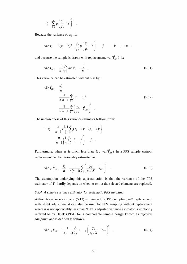
59

.1

2

2 ∑=

-=

N

l l

llz Y

p

Yps

Because the variance of kz is:

( ) .,1)(var1

2

2

2 n,kYp

YpYzEz

N

gz

l

llkk L==

-=-= ∑

=

s

and because the sample is drawn with replacement, )ˆvar( HHY is:

( ) ( ) .var1ˆvar

2

12 n

zn

Y zn

kkHH

s== ∑=

(5.11)

This variance can be estimated without bias by:

( )

( ) ( )

( ) ∑

∑

=

=

-

-=

--

=

=

n

kHH

k

k

n

ksk

zHH

Yp

y

nn

zznn

n

sY

1

2

1

2

2

.ˆ1

1

11

ˆrav

(5.12)

The unbiasedness of this variance estimator follows from:

( )

.1

1

)()(1

1

22

1

2

2

1

22

zz

n

kz

s

n

kkz

nnn

n

YzYzn

En

nsE

sss =

--

=

---

-=

∑

∑

=

=

Furthermore, when n is much less than N , )ˆvar( HTY in a PPS sample without

replacement can be reasonably estimated as:

( ) .ˆ/)1(

1ˆrav1

22

∑=

-

-==

n

kHT

k

kzHTHH Y

Xx

y

nnn

sY (5.13)

The assumption underlying this approximation is that the variance of the PPS

estimator of Y hardly depends on whether or not the selected elements are replaced.

5.3.4 A simple variance estimator for systematic PPS sampling

Although variance estimator (5.13) is intended for PPS sampling with replacement,

with slight adjustment it can also be used for PPS sampling without replacement

where n is not appreciably less than N. This adjusted variance estimator is implicitly

referred to by Hájek (1964) for a comparable sample design known as rejective

sampling, and is defined as follows:

( ) ( ) .ˆ/

1)1(

1ˆrav1

2

∑=

--

-=

n

kHT

k

kkHTHaj Y

Xx

y

nnY p (5.14)

60

The variance formula derived by Hájek (1964, p 1520) for rejective sampling is

( ) ( )

( )( )

.1

1

/

/1

1ˆvar

11

*

1

2

*2

∑∑

∑

==

=

−−==

−−=

N

kN

k kk

kkk

k

kk

N

k k

kkkHTHaj

Xx

yY

YXx

y

nY

ππππαα

ππ

Variance estimator (5.14) can be used in PPS without replacement under the

condition that the elements of the population are first put in a random order before

the systematic PPS sample is drawn. It can also be used when n and N are of the

same order of magnitude, provided kk XY / and kX are not correlated. If kk XY / and

kX are correlated and n and N are also of the same order of magnitude, it would

be better to use the following variance estimator:

( ) ( )

( )

( ).

1

/1

ˆ

ˆ/

1)1(

1ˆrav

1

1*

1

2

*2

∑

∑

∑

=

=

=

−

−=

−−

−=

n

k k

n

kk

kk

n

k k

kkHTHaj

Xx

y

Y

YXx

y

nnY

π

π

π

See Knottnerus (2011a) for a comparison of the variances of the HT estimator in

systematic PPS sampling and the ratio estimator in combination with SRSWOR

sampling. Finally, if / Nnk =π or ,/ NXxk = (5.14) becomes the familiar

estimator (2.12) for the variance of the direct estimator .ˆsSRSWOR yNY =

5.4 Example

To gain an impression of the reduction in variance with systematic PPS sampling,

this section describes the details of estimating a (combined) price index of 70

companies based on a sample of size 9=n . The variance for systematic PPS

sampling is compared with that for SRSWOR. The price changes are derived from

the price observations of Prodcom 27 from December 2004 to December 2005. The

data are shown in Table 5.1. The example is taken from Knottnerus (2011a). The

two largest companies were omitted because their turnover share was greater than

1/9. They were observed in full as a separate stratum.

Consider now the following price index for N companies:

.)1(year basein k company ofsharerevenue the:

centper in periodstatedin thek company for changepricee th:

)70(

1

1

=

==

∑

∑

=

=

N

kkk

k

N

kkk

WW

P

NPWI

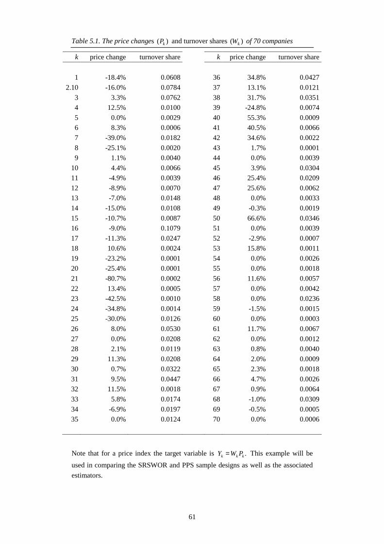
61

Table 5.1. The price changes )( kP and turnover shares )( kW of 70 companies

k price change turnover share k price change turnover share

1 -18.4% 0.0608 36 34.8% 0.0427

2.10 -16.0% 0.0784 37 13.1% 0.0121

3 3.3% 0.0762 38 31.7% 0.0351

4 12.5% 0.0100 39 -24.8% 0.0074

5 0.0% 0.0029 40 55.3% 0.0009

6 8.3% 0.0006 41 40.5% 0.0066

7 -39.0% 0.0182 42 34.6% 0.0022

8 -25.1% 0.0020 43 1.7% 0.0001

9 1.1% 0.0040 44 0.0% 0.0039

10 4.4% 0.0066 45 3.9% 0.0304

11 -4.9% 0.0039 46 25.4% 0.0209

12 -8.9% 0.0070 47 25.6% 0.0062

13 -7.0% 0.0148 48 0.0% 0.0033

14 -15.0% 0.0108 49 -0.3% 0.0019

15 -10.7% 0.0087 50 66.6% 0.0346

16 -9.0% 0.1079 51 0.0% 0.0039

17 -11.3% 0.0247 52 -2.9% 0.0007

18 10.6% 0.0024 53 15.8% 0.0011

19 -23.2% 0.0001 54 0.0% 0.0026

20 -25.4% 0.0001 55 0.0% 0.0018

21 -80.7% 0.0002 56 11.6% 0.0057

22 13.4% 0.0005 57 0.0% 0.0042

23 -42.5% 0.0010 58 0.0% 0.0236

24 -34.8% 0.0014 59 -1.5% 0.0015

25 -30.0% 0.0126 60 0.0% 0.0003

26 8.0% 0.0530 61 11.7% 0.0067

27 0.0% 0.0208 62 0.0% 0.0012

28 2.1% 0.0119 63 0.8% 0.0040

29 11.3% 0.0208 64 2.0% 0.0009

30 0.7% 0.0322 65 2.3% 0.0018

31 9.5% 0.0447 66 4.7% 0.0026

32 11.5% 0.0018 67 0.9% 0.0064

33 5.8% 0.0174 68 -1.0% 0.0309

34 -6.9% 0.0197 69 -0.5% 0.0005

35 0.0% 0.0124 70 0.0% 0.0006

Note that for a price index the target variable is .kkk PWY = This example will be

used in comparing the SRSWOR and PPS sample designs as well as the associated

estimators.

62

The standard estimator for a price index based on SRSWOR is a pure ratio estimator

defined as:

.ˆ

1

1

∑∑

=

== n

k k

n

k kkSRSWOR

w

pwI (5.15)

Although ratio estimation is discussed below in Chapter 6, the frequently used

approximation for the variance of an estimated ratio is given here:

( )

( ).

1var

/1

/1var

varˆvar

1

1

1

1

1

-=

-=

=

∑

∑∑

∑∑

=

=

=

=

=

n

k s

kk

n

k k

n

k kk

n

k k

n

k kkSRSWOR

w

Ipw

n

Iwn

pwn

w

pwI

Because the variance of the denominator in the above expression is relatively small

in comparison with the volatility of the numerator, the denominator is usually

replaced with the population mean of the kW , i.e. N/1 . This gives:

( ) ( )

( ) .1

11

1varˆvar

1

222

1

2

∑

∑

=

=

-

-

-=

-=

N

kkk

n

kkkSRSWOR

IPWNN

n

n

N

Ipwn

NI

(5.16)

In the second part of (5.16) formula (2.12) was used with:

( ) .0=Ù-= pkkk YIPWY

Applying this formula to the 70 price changes in Table 5.1, gives:

( ) .101ˆvar =SRSWORI (5.17)

Had sampling been with replacement, then the variance without finite population

correction would be:

( ) .116ˆvar =SRSWRI

In other words, the finite population correction is 87.0)1( =- f .

The variance formulas in (5.16) and (5.17) will now be compared with the variance

of a second estimator based on systematic PPS sampling, where the inclusion

probabilities are proportional to the .kW As seen at the start of Section 5.3.3,

.nWkk =p

The PPS estimator of I now equals in accordance with (5.3):

63

.1ˆ

111∑∑∑

===

====n

ksk

n

k k

kkn

k k

kPPS pp

nnw

pwyI

p

In other words, in PPS sampling the weighted mean of the separate price changes in

the population is estimated with the unweighted mean of the price changes in the

sample.

We first examine the variance for PPS sampling with replacement. Formula (5.11)

in this example becomes:

( ) ( ) .441ˆvar

1

22

=-== ∑=

N

kkk

zPPSHH IPW

nnI

s

We then examine the result of the variance approximation that underlies (5.14):

( ) ( )( )

( )( ) .2911

11ˆvar

1

2

1

2

2

=--=

--=

∑

∑

=

=

N

kkkk

N

kkkkPPS

IPnWWn

IPn

I pp

In other words, in PPS sampling the finite population correction of 66.0 ( 44/29= )

is again much less than that of 87.0 for SRSWOR. Table 5.2 lists the various

variances.

Table 5.2. Variances in various sample designs

with replacement without replacement

SRS 116 101

PPS 44 29

Finally, we point out that a simulation in which 000,20 systematic PPS samples of

size 9=n were selected from a population of 70 companies with a different random

sequence on each occasion yielded a variance of 30 for PPSI . In other words, (5.14)

in this situation is an almost unbiased variance estimator. This example also

illustrates once more that the reduction in variance in systematic PPS sampling

compared with SRSWOR can be substantial, up to approximately %70 .


Quality indicators for PPS sampling are:


- the size of nonresponse;

- the randomness of the sequence of the elements in the population and the

degree of dependence between kk XY / and kX .

64

Nonresponse can severely affect the quality of the results if (i) the size of the

nonresponse is large and (ii) the nonresponse is selective. Part of the bias from

selective nonresponse can sometimes be corrected by using auxiliary variables that

correspond with both the probability of response and the target variable.

Another important assumption in random sampling is that the frame from which the

sample is drawn corresponds closely with the target population about which

inferences are to be made.

The above focused in particular on PPS sampling in which the elements are, or may

be considered to be, in random order. If there is no appreciable relation between

kk XY / and k ( Nk ,,1 L= ), a random ordering of the population will have no

systematic effect on the findings that we observed earlier in Section 5.1.2. Therefore

a random order is not absolutely necessary in situations of this kind. If the elements

remain in a fixed sequence, the samples must not be allowed to become

homogeneous in terms of the )./(*kkk YY π≡

5.6 Appendix

For the N selection indicators, by definition:

.11

naaa N

N

kk =++=∑

=

L

Taking the expectation on both sides gives:

.1

nN

kk =∑

=

π

Likewise by definition:

( ) .1 kNk anaaa =++L

Again, taking the expectations on either side immediately gives:

.1

k

N

lkl nππ∑

=

=

These two results will be needed below in this section.

Proof of (5.7)

For selection indicator ka :

( ) ( )( )( ) ( )( ) 22

22

2var

kkkk

kk

kkk

aE

aEaE

aEaEa

πππ −=−=

−=

−=

and:

65

( ) ( )( ) ( )( )( )( ) ( ) ( )

.

,cov

lkkl

kklk

llkklk

aEaEaaE

aEaaEaEaa

πππ −=−=

−−=

QED.

Proof of (5.8)

It follows from (5.7) and the definition of the HT estimator of the population total –

see (5.5) – that its variance is:

( )

.

)()1(ˆvar

1 1

1 12

2

1

∑∑

∑∑∑

= =

=≠==

−=

−+−=

N

k

N

llk

lk

lkkl

N

k

N

kll lk

lklkkl

k

kN

kkkHT

YY

YYYY

πππππ

πππππ

πππ

QED.

The following results can be proved for estimators (5.9) and (5.10):

( )( ) ( ) ( )( ) ( ) .ˆvarˆravˆvarˆrav HTHTSYGHTHTHT YYEYYE =∧=

The proofs are as follows. The HT estimator )ˆr(av HTY (see (5.9)) is rewritten in

terms of the selection indicators as:

( ) .ˆrav1 11 1∑∑∑∑

= == =

−=

−=

N

k

N

llk

lkkl

lkkllk

n

k

n

llk

lkkl

lkklHTHT YYaayyY

ππππππ

ππππππ

The unbiasedness of the variance estimator now follows from the property:

kllk aaE π=)( (see (2.9)). It is possible to calculate that:

( )( ) ( )

( ) .ˆvar

ˆrav

1 1

1 1

1 1

∑∑

∑∑

∑∑

= =

= =

= =

=

−=

−×=

−=

N

k

N

lHTHTlk

lk

lkkl

N

k

N

llk

lkkl

lkklkl

N

k

N

llk

lkkl

lkkllkHTHT

YYY

YY

YYaaEYE

πππππ

πππππππ

ππππππ

A condition for unbiasedness is again that klπ<0 Nlk ≤≤ ,1 .

Because kllk aaE π=)( , estimator (5.10) as such is an unbiased estimator of :

( ) ( )∑∑= =

−−−=

N

k

N

l l

l

k

klkklHTSYG

YYY

1 1

2

2

1ˆvarππ

πππ

provided klπ<0 . In other words:

66

( )( ) ( ) .2

1ˆrav1 1

2

∑∑= =

−−−=

N

k

N

l l

l

k

klkklHTSYG

YYYE

πππππ

Expanding the squared term on the right-hand side of the above equation and using

the two properties of the selection indicators that were derived at the start of this

section, nN

k k =∑ =1π and k

N

l kl nππ =∑ =1, again yields:

( )( ) .ˆrav1 1∑∑

= =

−=

N

k

N

llk

lk

lkklHTSYG YYYE

πππππ

In other words, estimator (5.10) is also an unbiased estimator of (5.8).

67

6. Ratio estimator


Chapter 2 showed that the sample mean is an unbiased estimator of the population

mean. It is also referred to as the direct estimator of Y , because it uses only the

observed values of the variable Y . Later chapters showed how the precision of an

estimator can be improved by incorporating available information about the

population into the sampling design. For instance, Chapter 3 used auxiliary

information to divide the population into homogeneous groups, or strata, from

which separate samples can then be drawn. Chapter 5 showed that auxiliary

information about the size of the elements makes it possible to select elements with

unequal probabilities. This and the following two chapters show how auxiliary

information can be used in the estimation procedure. Different types of auxiliary

information result in different estimators. We introduce some commonly used

alternative estimators of the population mean (or total) for the simplest sampling

design: simple random sampling (without replacement). The discussion is restricted

to estimation methods that involve one auxiliary variable. As with stratified

sampling and sampling with unequal probabilities, the use of auxiliary information

leads to more precise estimators if the relation between target variables and auxiliary

variables is sufficiently strong.

So far we have discussed the most important building blocks of sample surveys:

simple random sampling, stratification, clustering, and sampling with unequal

probabilities. Ratio and regression estimators are discussed below. Most sampling

designs used at Statistics Netherlands consist of multiple building blocks. The

formulas for the estimators, and in particular those for the standard errors, can then

become extremely complex. In practice, weights are used to obtain point estimates

of parameters, which usually simplifies matters considerably. The weights can be

determined automatically using the Bascula software package, which also has

various functions for calculating variances. The remaining chapters briefly discuss

the relationship between estimating and weighting.

6.2 Applicability

The ratio estimator is a relatively simple and widely used alternative for the direct

estimator discussed in Chapter 2. The thinking behind the ratio estimator, which

uses a quantitative auxiliary variable, is that the ratio kk XY / of the values of the

target variable and the auxiliary variable in the population varies less than the target

variable itself.

An example is turnover per employee. If this ratio varies little from one business to

another, it can be used to estimate total turnover in the Netherlands. The procedure

would be to estimate the ratio based on a sample and then multiply the estimated

ratio by the number of employees in the Netherlands.

68


The limited variation of the ratio of the target variable Y and the auxiliary variable

X can be expressed as:

BX

Y

k

k ≈ or kk BXY ≈

where B is a constant. The points ),( kk YX lie approximately on a straight line

through the origin, which is referred to as the regression line (see Figure 6.1). If the

regression line is a good description of the set of points, the individual values of Y

can be predicted satisfactorily based on X . And because we have population

information on X it would be logical to incorporate it into the estimator.

Figure 6.1. Linear relationship between Y and X through the origin

200 400 600 800

500

1000

1500

X

Y

X

Y

Summing all the elements of the population and dividing by N gives:

.XBY =

If the population mean X is known, and the value of B is available, Y can then be

estimated as XB . The ideal value for B is evidently XY / , but this cannot be

calculated, because it assumes knowledge of Y . However, this value can be

estimated from the sample data using:

.ˆ

ˆˆ

X

Y

x

ybB

s

s ===

69

This expression gives the ratio estimator QTY for the population mean Y :

.ˆ Xx

yXbY

s

sQT == (6.1)

For the ratio estimator the sample mean sy is multiplied by a term sxX / , which

adjusts for the difference between the sample mean and the population mean of the

auxiliary variable. The assumption here is that the adjustment can also be projected

onto the target variable, since there is a relation between the target variable and the

auxiliary variable. Figure 6.2 shows how the ratio estimator works.

Figure 6.2. The ratio estimator

200 400 600 800

500

1000

1500

X

Y

xs =X

Y^

QT =ys

xs

Y^

QT

Figure 6.2 shows that a ratio estimate is obtained by adding a term )( sxXb − to the

sample mean sy , where ss xyb /= , is the slope of the regression line. Therefore the

ratio estimator (6.1) can also be written as:

.)(ˆ XbxXbyY ssQT =−+=

Note that by setting XY = the ratio estimator equals X . Regarding the auxiliary

variable, the sample outcome is therefore consistent with the population, which is a

very desirable property in practice. It enables us to align different statistics by using

the same auxiliary variable.

The ratio estimator in (6.1) can also be written in terms of weights. That is,

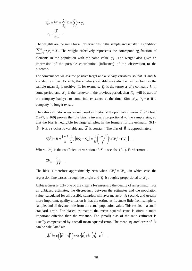
70

.

ˆ

1

sk

n

kkk

s

sQT

xn

Xw

ywXx

yXbY

=

=== ∑=

The weights are the same for all observations in the sample and satisfy the condition

.1

Xxwn

k kk =∑ = The weight effectively represents the corresponding fraction of

elements in the population with the same value .ky The weight also gives an

impression of the possible contribution (influence) of the observation to the

outcome.

For convenience we assume positive target and auxiliary variables, so that B and b

are also positive. As such, the auxiliary variable may also be zero as long as the

sample mean sx is positive. If, for example, kY is the turnover of a company k in

some period, and kX is the turnover in the previous period, then kX will be zero if

the company had yet to come into existence at the time. Similarly, 0=kY if a

company no longer exists.

The ratio estimator is not an unbiased estimator of the population mean Y . Cochran

(1977, p 160) proves that the bias is inversely proportional to the sample size, so

that the bias is negligible for large samples. In the formula for the estimator (6.1),

bB =ˆ is a stochastic variable and X is constant. The bias of B is approximately:

[ ] [ ] .1111

]ˆ[ 222 xyxxyx CVCVB

f

f

NSBS

Xn

fBBE −

−=−−≈−

Where xCV is the coefficient of variation of X – see also (2.1). Furthermore:

.YX

SCV xy

xy =

The bias is therefore approximately zero when xyx CVCV =2 , in which case the

regression line passes through the origin and kY is roughly proportional to kX .

Unbiasedness is only one of the criteria for assessing the quality of an estimator. For

an unbiased estimator, the discrepancy between the estimates and the population

value, calculated for all possible samples, will average zero. A second, and usually

more important, quality criterion is that the estimates fluctuate little from sample to

sample, and all deviate little from the actual population value. This results in a small

standard error. For biased estimators the mean squared error is often a more

important criterion than the variance. The (small) bias of the ratio estimator is

usually compensated by a small mean squared error. The mean squared error of B

can be calculated as:

( ) ( ) ( ) ( )( ) .ˆˆvarˆˆ 22BBEBBBEBG −+=

−=

71

When the bias of B is small relative to the standard error of B , the variance is a

good approximation of the mean squared error. Then (see e.g., Muilwijk, 1992,

Section 5.8.3):

( )BCVf

f

NBG x

ˆvar11

1)ˆ(

−+≤

so that the approximation is better for larger f and/or smaller xCV .

A good approximation for the variance of the ratio estimator of the population mean

is obtained from:

( ) ( ) .1

1

1ˆvar1

2∑=

−

−−

=

N

kkkQT BXY

f

f

NNY (6.2)

The variance is smaller as the relationship between Y and X is stronger, that is,

when the values kY deviate less from the regression line. However, it is impossible

to calculate the variance (6.2) because there are no population data of Y, but we can

nonetheless produce an estimate based on the sample. The variance estimator of

(6.2) is:

( ) .1

111ˆrav1

2

−−

−=

∑

=

n

kkkQT bxy

nf

f

NY (6.3)

For large samples the variance of the ratio estimator is usually less than that of the

direct estimator. It is even possible to determine the situations where this occurs.

Rewrite the variance of the ratio estimator as:

( ) ( ) .211ˆvar 222

xyxyQT BSSBSf

f

NY −+

−=

Comparing this variance with the variance for the sample mean in simple random

sampling – see (2.11) – gives:

( ) ( ) ( )( ) ,2

11

211ˆvarˆvar 2222

yxx

yxyxyQT

SBSBSf

f

N

SSBSf

f

NYY BS

ρ−

−=

−−+

−≈−

where ρ is the population correlation coefficient of X and Y. The ratio estimator is

therefore preferable to the direct estimator if:

.2

1

2

1 ρ<

=

y

x

y

x

CV

CV

S

SB

Therefore, if the coefficient of variation of X is more than twice as large as that of

Y, i.e. xy CVCV <2 , then the ratio estimator is less precise than the direct estimator

(even for a correlation of 1=ρ ). If the variable X equals the variable Y , but was

measured at an earlier time, then the coefficients of variation are approximately

72

equal and the ratio estimator is better than the direct estimator if ρ<5.0 . If all the

values of X are the same ),0( 2 =xS the ratio estimator corresponds with the direct

estimator for simple random sampling.

Again the ratio estimator of the population mean simply yields the ratio estimator of

the population total after multiplying by the population size:

.ˆ bXXbNYNY QTQT ===

The variance of this estimator can be calculated as:

( ) ( ) .1

1ˆvar

1

2∑=

−

−

−=

N

kkkQT BXY

f

f

N

NY

The ratio estimator of the population total can also be written in terms of weights:

.

ˆ

#

1

#

sk

n

kkk

s

sQT

xn

Xw

ywXx

yXNbY

=

=== ∑=

The weights #kw satisfy .

1

# Xxwn

k kk=∑ =

Analogous to the ratio estimator of the

mean, the weight now effectively represents the number of elements in the

population with the same value .ky For this reason the #kw are sometimes called

raising weights.

The ratio estimator is usually used to improve precision. The ratio estimator also

ensures the consistency of sample estimates with population numbers or totals for

the auxiliary variables (see also Chapter 8) and adjusts the estimator for

nonresponse. The parameter to be estimated can sometimes be a ratio (e.g. the

number of fatal traffic accidents in proportion to the total number of accidents). The

ratio estimator can also be used for estimating a total when the population size is

unknown. This is particularly relevant when producing estimates for subpopulations.

Sometimes several auxiliary variables correlate with the target variable Y , in which

case one auxiliary variable may be chosen, e.g. the one with the highest correlation.

Another option would be to employ more than one auxiliary variable using the

general regression estimator. Finally, we note that often nothing is known about the

relationship between Y and X in the population. If this is the case, we have to rely

on the sample data, provided the sample distribution with respect to Y is not skewed

due to chance or nonresponse. Information from earlier surveys can also help in

understanding the relation between Y and X . The ratio estimator is most

appropriate when a straight line through the origin is the best description of the

relationship between Y and X , and when the variance of the values kY about the

regression line are proportional to kX .

73

6.4 Example

A simple random sample of 8 towns is drawn from a population of 42 towns. Table

6.1 gives the population figures and the number of general practitioners for each

town. We have to estimate the total number of general practitioners in the

population. The number of general practitioners will be related to the number of

residents of a town, and the numbers of residents will therfore be used as auxiliary

information in the estimation proces. On average there are 23.5 general practitioners

in the 8 selected towns. Without using the auxiliary variable, the total number of

general practitioners is estimated at 987ˆ == yNY with a standard error of 80.48.

The mean number of residents in the population is 50, and in the sample 47.13. In

relation to the population the mean number of residents in the sample is therefore a

little too low, and this is probably also true of the mean number of general

practitioners in the sample.

The estimate of the total number of general practitioners in the population using the

ratio estimator is:

.1,0472,1000.499ˆ =×== Xx

yY

s

sQT

The standard error of the estimator is:

( ) ( )

.08.5468.11410.042

1

11ˆˆ

2

1

22

=××=

−−

−= ∑=

n

kkkQTe bxy

nn

fNYS

Table 6.1 Population and number of general practitioners in a sample of 8 towns

TownResidents

(x1000)

General

practitioners 2)( kk bxy −

1 38 20 1.102.10 52 23 8.59

3 75 35 5.764 32 20 16.345 60 28 3.696 43 25 12.657 57 22 41.278 20 15 25.27

Total 377 188 114.68


Quality indicators for the ratio estimator are:


74


- the size of the sample.


large and (ii) the nonresponse is selective. The bias from selective nonresponse can

sometimes be corrected by using auxiliary variables that correspond with both the

probability of response and the target variable, like the ratio estimator described in

this ch apter.

Another important assumption in employing the ratio estimator is that the size of the

sample is sufficiently large to ensure that the bias of the ratio estimator and the

corresponding variance estimator remain limited.

75

7. Regression estimator


When the relationship is linear, but does not pass through the origin, it is better to

use the regression estimator rather than the ratio estimator – see Figure 7.1. The

relationship between Y and X is now given by:

kk BXAY +≈ (7.1)

where A and B are nonzero constants. These constants are referred to as the

regression coefficients.

Figure 7.1. Linear relationship between Y and X

0 100 200 300 400 500 600 700

050

010

0015

00

X

Y

X

Y

This linear relationship is the starting point for the regression estimator. Section 7.3

describes the regression estimator in more detail.

7.2 Applicability

The regression estimator and its variants are frequently used in socioeconomic

statistics. The usual source of auxiliary variables is the Municipal Personal Records

Database (GBA). The Repeated Weighting subtheme (part of the theme ‘Sampling

theory’ of the Methods Series; Gouweleeuw and Knottnerus, 2008) also uses the

regression estimator, albeit with a rather different purpose. The regression estimator

is also often used in other themes

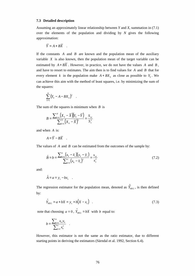
76


Assuming an approximately linear relationship between Y and X, summation in (7.1)

over the elements of the population and dividing by N gives the following

approximation:

.XBAY +≈

If the constants A and B are known and the population mean of the auxiliary

variable X is also known, then the population mean of the target variable can be

estimated by XBA + . However, in practice, we do not have the values A and B ,

and have to resort to estimates. The aim then is to find values for A and B that for

every element k in the population make kBXA + as close as possible to kY . We

can achieve this aim with the method of least squares, i.e. by minimizing the sum of

the squares:

( ) .1

2∑=

−−N

kkk BXAY

The sum of the squares is minimum when B is

( )( )( ) 2

1

21

x

xy

N

k k

N

k kk

S

S

XX

YYXXB =

−

−−=

∑∑

=

=

and when A is:

.XBYA −=

The values of A and B can be estimated from the outcomes of the sample by:

( )( )( ) 2

1

21ˆ

x

xyn

k sk

n

k sksk

s

s

xx

yyxxbB =

−

−−==

∑∑

=

= (7.2)

and:

.ˆss xbyaA −==

The regression estimator for the population mean, denoted as REGY , is then defined

by:

( ) .ˆssREG xXbyXbaY −+=+= (7.3)

note that choosing 0=a , XbYREG =ˆ with b equal to:

.1

2

1

∑∑

=

== n

k k

n

k kk

x

yxb

However, this estimator is not the same as the ratio estimator, due to different

starting points in deriving the estimators (Särndal et al. 1992, Section 6.4).

77

As with the ratio estimator the regression estimator is an adjustment to the sample

mean sy – see Figure 7.2. Adjustment occurs as soon as there is a difference

between the population mean and the sample mean of the auxiliary variable X .

Figure 7.2. The regression estimator

0 100 200 300 400 500 600 700

050

010

0015

00

X

Y

xs =X

Y^

REG =ys

xs

Y^

REG

By analogy with the ratio estimator, the regression estimator of the population mean

can also be written in terms of weights. Substituting (7.2) into (7.3) gives:

( )( )( )

.1

ˆ

1

2

1

∑

∑

=

=

−−−+=

=

n

k sk

sskk

n

kkkREG

xx

xXxx

nw

ywY

As with the ratio estimator, the weights kw satisfy Xxwn

k kk =∑ =1.

The regression estimator is not an unbiased estimator of the population mean,

because b is not an unbiased estimator of B . The bias of REGY amounts to

),ˆ(cov xB− , where )cov(⋅ stands for covariance. As with the ratio estimator, the bias

of the regression estimator is inversely proportional to sample size, so that it

becomes negligible for large samples. If the regression line passes through all points

),( kk YX , then BB =ˆ for each possible sample and 0),ˆ(cov =xB . The bias in this

situation is zero. The variance of the regression estimator can be well approximated

by:

78

( ) ( )( ) .1

1

1ˆvar1

2∑=

−−−

−−

=

N

kkkREG XXBYY

f

f

NNY

The variance is determined by the variation in Y that cannot be explained by X ,

which is referred to as the residual sum of squares. The residual for element k ,

denoted by ke , is defined by:

( ) ( ) .XXBYYBXAYe kkkkk −−−=+−=

The more variation in Y can be explained by X , the stronger the relationship

between Y and X , and the smaller the variance. A different way of achieving this

result is to rewrite the variance as:

( ) ( ) ( ) ( ) .var11

11ˆvar 222 yS

f

f

NY yREG ρρ −=

−−=

The closer the population correlation coefficient to 1+ or 1− , the smaller the

variance will be. The variance is always a factor )1( 2ρ− smaller than the variance

of the direct estimator. If there is no relationship between Y and X , i.e. 0=ρ , then

the variance of the regression estimator equals that of the direct estimator, in which

case it would be pointless to use X as a auxiliary variable.

An estimator of the variance of the regression estimator based on the sample is:

( ) ( )( ) .1

111ˆrav1

2

−−−

−

−= ∑=

n

kskskREG xxbyy

nf

f

NY

A regression estimator for the population total can be derived directly from

regression estimator (7.3) of the population mean:

( ) .ˆˆssREGREG xXNbyNYNY −+==

This regression estimator for the population total can also be rewritten in terms of

weights:

( )( )

.)(

ˆ

1

2

#

1

#

∑

∑

=

=

−−−+=

=

n

k sk

ssk

n

kkkREG

xx

xXxxN

n

Nw

ywY

k

The weights in this regression estimator satisfy the condition .1

# Xxwn

k kk=∑ =

See

Camstra and Nieuwenbroek (2002) and the series topic on Repeated weighting, for

weights where there are two or more auxiliary variables.

The variance of the regression estimator of the population total can be calculated as

follows:

( ) .ˆvarˆvar 2

= REGREG YNY

79

The regression estimator is usable with both positive and negative correlation; kY

and kX can also assume zero or negative values.

7.4 Example

Examination of the sample data from Example 6.4 raises the suspicion that although

it is linear, the relationship between the number of residents and number of general

practitioners for each town cannot be expressed as a regression line through the

origin. It would then seem to be logical to apply the regression estimator. The

sample parameters are:

.97.95

24.3650.23

13.30413.472

2

=

==

==

xy

y

x

s

sy

sx

The estimates of the regression coefficients are:

.66.831.02

=−=∧== xbyas

sb

x

xy

The regression estimate of the total number of general practitioners is therefore:

98714.84)(8.6642)(ˆ =+×=+= XbaNYREG

which corresponds with the estimate obtained by applying the direct estimator. The

standard error of the regression estimator of the total is:

( ) ( )( )

.05.3582.4271

)42/8()42/8(1

42

1

11ˆˆ1

2

=

××

−×=

−−−−

−= ∑=

n

kskskREGe xxbyy

nf

fNYS

The standard error is, therefore, somewhat less than the standard error of the direct

estimator and also less than the standard error of the ratio estimator. For large

samples the regression estimator is never worse than the ratio estimator.


Quality indicators for the regression estimator closely resemble those of the ratio

estimator:



- the number of auxiliary variables;

- the size of the sample.


large and (ii) the nonresponse is selective. Part of the bias from selective

nonresponse can sometimes be corrected by using the regression estimator described

80

in this chapter with auxiliary variables that correspond with both the probability of

response and the target variable.

Another important assumption in the regression estimator is that the size of the

sample is sufficiently large to ensure that the bias of the regresssion estimator and

the bias of its variance estimator remain limited. Unlike the ratio estimator, it is also

important with the regression estimator that the number of auxiliary variables in the

model is not too large in proportion to the number of observations. For reasons of

simplicity this section is restricted to the case of one auxiliary variable, but in

practice many more auxiliary variables can be included in the regression model,

depending on the size of the sample.

81

8. Poststratified estimators


A poststratification estimator is obtained when the population is divided into

poststrata after SRSWOR (see Chapter 2) is carried out. The sample is also divided

in accordance with the poststrata. In other words, the sample size for each

poststratum is stochastic in nature, which is the essential difference with ordinary

(pre)stratification.

8.2 Applicability

Poststratification is used regularly when it is not known in advance to which stratum

each element of the population belongs, or if no account was taken in the sampling

design of the (relevant) stratification. For example, when surveying the financial

situation of young adolescents, where there is no precise knowledge of whether the

subjects are students, employed, or unemployed. This lack of knowledge hampers

prior stratification. Once sampling has taken place, the selected elements can be

divided into the different strata, which is known as poststratification. However,

precautions must be taken to limit the probability of having strata without sample

observations, which means not choosing excessively small strata. If empty strata

occur in practice, nonetheless, it is still possible to combine strata.


8.3.1 The standard poststratified estimator

Unlike the ratio estimator and the regression estimator, the poststratified estimator

uses only qualitative (categorical) auxiliary variables, such as gender, region and

marital status. Suppose that the population is divided according to a qualitative

auxiliary variable into L disjunct groups. After observing the value of the auxiliary

variable, it can be established for each element in the population to which group

(poststratum) it belongs. The number of elements in the sample that belong to

poststratum l is denoted with ln for .,,1 Ll L= The number of elements in the

population in poststratum l is lN (this number must be known). To distinguish the

poststrata from the standard prestrata, subscript l is used for the lth poststratum

),,1( Ll L= and subscript h for the hth standard prestratum ).,,1( Hh L= The

poststratification estimator of the population mean Y is

l

L

l

lpost y

N

NY ∑

=

=1

ˆ . (8.1)

The poststratification estimator is unbiased under the condition that every

poststratum has at least one observation. At first glance, the estimator appears to be

the same as the direct estimator for a stratified sample. However, there is a

conceptual difference. The sample size in a poststratum is stochastic; the number of

82

sample elements that will end up in the poststratum is unknown before the sample is

drawn. For a (pre)stratified sample, the exact number of sample elements per

stratum is determined beforehand. The stochastic nature of the sample size per

poststratum is expressed in the variance of the poststratification estimator. For large

samples the variance can be well approximated as:

.111ˆvar

1

22

1

2 ∑∑==

--+-=

L

ll

lL

ll

lpost S

N

N

n

fS

N

N

n

fY (8.2)

The first term in the variance formula is the variance for prestratification and

proportional allocation. The second term reflects the uncertainty about the sample

sizes of the poststrata. This term can be interpreted as the additional contribution to

the variance because the allocation that is realized differs from the proportional

allocation. The more homogeneous the strata with respect to the target variable, i.e.

the smaller the differences between the values of the target variable within a

stratum, the smaller the variance of the poststratification estimator. It is therefore

important to select the poststrata such that the variation of the target variable

manifests itself mainly in the differences between the strata. The estimator for the

variance is obtained by replacing 2lS in (8.2) by the sampling equivalents 2

ls .

8.3.2 The poststratified estimator for complex sampling designs

Poststratification often assumes one or more categorical auxiliary variables X that

divide the population into L categories (poststrata), each with lN elements. The

population total of Y in poststratum Ll ,,1L= can be estimated with the Horvitz-

Thompson estimator:

∑=

=ln

k lk

lklHT

yY

1,

ˆp

where ln is the number of elements in the sample that belong to poststratum l , and

lkp is the inclusion probability of element k in stratum l. Likewise the population

size lN of poststratum l can be estimated with:

∑=

=ln

k lklHTN

1,

1ˆp

so that an estimator for lY is:

.ˆ

ˆˆ

,

,

lHT

lHTl

N

YY =

The poststratified estimator of the total is then:

.ˆ

ˆ1 1,

∑ ∑= =

=L

l

n

k lk

lk

lHT

lpost

l y

N

NY

p

83

Note that L different correction weights are involved, and that in a poststratum l

they equal lHTl NN ,ˆ/ . The poststratification estimator is approximately unbiased.

Although it is possible to give a good approximation formula of the variance, it

sheds little light on a specific sampling design. The discussion of the

poststratification estimator is therefore restricted to stratified sampling, omitting

formulas.

Poststratification with a stratified sample

Suppose the population is divided into H strata and we have selected a stratified

sample with hn elements in each stratum. We distinguish four cases that may occur

in practice.

(a) The strata and the poststrata coincide (i.e. LH = ).

(b) The poststrata are unions of strata. An example is if municipalities form the

strata and country regions the poststrata.

1 2 H (strata)

1 2 L (poststrata)

Poststrata are unions of strata

(c) The poststrata are parts of strata. An example is if regions form the strata

and the municipalities the poststrata.

1 2 H (strata)

1 2 L (poststrata)

Poststrata are parts of strata

84

(d) The poststrata cross the strata. An example is if regions form the strata and

the poststrata are determined by gender, or by age groups.

1 H (strata)

1

..

..

L

(poststrata)

Poststrata cross strata

Note to (a)Here the direct estimator (HT estimator) for stratified sampling (see Chapter 3) is

appropriate. The associated variance also follows from Chapter 3.

Note to (b)Poststratification adds nothing in this case, because the stratification has finer

categories than the poststratification. ll NN =ˆ for all l , therefore the direct estimator

for stratified sampling is again applicable.

Note to (c)

Poststratification is applied in stratum h of the simple random sample with, say hL

strata. Therefore, the variance of the poststratified estimator for simple random

sampling applies within each stratum. Because the strata are sampled independently,

these variances must be summed to obtain the variance of the poststratified

estimator (with L poststrata).

Note to (d)For each poststratum, the direct estimator for stratified sampling is used to estimate

the total of the target variable and the population size per poststratum. Subsequently

the means of the target variable in the poststrata can be estimated, which are then

weighted with the actual population size of the poststrata, and summed; see Särndal

et al. (1992, p. 268).

8.4 Example

A researcher is interested in the financial situation of students. He has access to

university records with 000,5 students, from which he selects 500 through

SRSWOR. One of the questions is about whether someone has paid work for more

than 10 hours a week alongside their study. The sample consists of 300 male and

200 female students, of which 105 men and 50 women reported having a paid job of

more than 10 hours a week. If the researcher were to use only the information from

the sample, he would estimate that

85

550,1155500

000,5 =×

students have paid work for more than 10 hours a week.

The university records also have information about student gender; in total there are

300,3 male and 700,1 female students registered at the university. It then follows

that, relative to the student population, the male students are underrepresented, and

the female students overrepresented, in the sample. Because we suspect that a

student's gender is related to having a paid job of more than 10 hours a week, we

would prefer a sample that is representative in terms of the numbers of male and

female students. In the current situation in which sampling already has occurred, the

estimator can only be adjusted for underrepresentation and overrepresentation with

hindsight (a posteriori).

Therefore a better estimate of the number of students with a paid job is :

580,1700,1200

50300,3

300

105 =×+× .


An important quality indicator for the poststratification estimator is the margin of

uncertainty. As long as all the strata have sufficient elements there is little cause for

concern. When, however, some strata have almost no observations, the variance of

the poststratification estimator may increase. In order to avoid this, it is

recommended to combine strata.

86

9. References

Camstra, A. and Nieuwenbroek, N.J. (2002), Syllabus for the sampling theory

course. CBS-Academie, Voorburg.

Cochran, W.G. (1977), Sampling Techniques. John Wiley & Sons, New York.

Gouweleeuw, J.M. and Knottnerus, P. (2008), Theme: Sampling Theory, Subtheme:

Repeated Weighting. Methods Series document, Statistics Netherlands,

Voorburg [English translation from Dutch in 2012].

Hájek, J. (1964), Asymptotic theory of rejective sampling with varying probabilities

from a finite population. Annals of Mathematical Statistics 35, 1491-1523.

Hansen, M.H. and Hurwitz, W.N. (1943), On the theory of sampling from finite

populations. Annals of Mathematical Statistics 14, 333-362.

Horvitz, D.G. and Thompson, D.J. (1952), A generalization of sampling without

replacement from a finite universe. Journal of the American Statistical

Association 47, 663-685.

Knottnerus, P. (2003), Sample Survey Theory: Some Pythagorean Perspectives.

Springer-Verlag, New York.

Knottnerus, P. (2011a), On the efficiency of randomized PPS sampling. Survey

Methodology, 37, 95-102.

Knottnerus, P. (2011b), Simple derivations of variance formulas in two-stage simple

random sampling, Discussion paper, Statistics Netherlands, The Hague.

Muilwijk, J., Snijders, T.A.B. and Moors, J.J.A. (1992), Kanssteekproeven (Random

sampling). Stenfert Kroese, Leiden.

Särndal, C.E, Swensson, B. and Wretman, J.H. (1992), Model Assisted Survey

Sampling. Springer-Verlag, New York.

Sen, A.R. (1953), On the estimate of the variance in sampling with varying

probabilities. Journal of the Indian Society of Agricultural Statistics 5, 119-127.

Yates, F. and Grundy, P.M. (1953), Selection without replacement from within

strata with probability proportional to size. Journal of the Royal Statistical

Society B, 15, 253-261.

87

Version history

Version Date Description Authors Reviewers

Dutch version: Steekproeftheorie / Steekproefontwerpen en Ophoogmethoden

1.0 26-02-2010 First Dutch version Reinder BanningAstrea CamstraPaul Knottnerus

Kees van BerkelJosé GouweleeuwSander ScholtusIlona Verburg

2.0 29-02-2012 Major changes in chapter 4

Reinder BanningAstrea CamstraPaul Knottnerus

Sander Scholtus

English version: Sampling theory / Sampling design and Estimation methods

2.0E 29-02-2012 First English version Reinder BanningAstrea CamstraPaul Knottnerus

Sampling theory - CBS Netherlands Statistics Methods (201207) Sampling theory Sampling design and...

Documents

Transcript of Sampling theory - CBS Netherlands Statistics Methods (201207) Sampling theory Sampling design and...