Sampling Probability and Inference - SAGE … Probability and Inference ... This chapter provides an...
27
[12:10 28/12/2007 5068-Mazzocchi-Ch05.tex] Job No: 5068 Mazzocchi: Statistics for Consumer Research Page: 103 103–129 PART II Sampling Probability and Inference The second part of the book looks into the probabilistic foundation of statistical analysis, which originates in probabilistic sampling, and introduces the reader to the arena of hypothesis testing. Chapter 5 explores the main random and controllable source of error, sampling, as opposed to non-sampling errors, potentially very dangerous and unknown. It shows the statistical advantages of extracting samples using probabilistic rules, illustrating the main sampling techniques with an introduction to the concept of estimation associated with precision and accuracy. Non-probability techniques, which do not allow quantification of the sampling error, are also briefly reviewed. Chapter 6 explains the principles of hypothesis testing based on probability theories and the sampling principles of previous chapter. It also explains how to compute confidence intervals and how statistics allow one to test hypotheses on one or two samples. Chapter 7 extends the discussion to the case of more than two samples, through a class of techniques which goes under the name of analysis of variance. The principles are explained and with the aid of SPSS examples the chapter provides a quick introduction to advanced and complex designs under the broader general linear modelling approach.
Transcript of Sampling Probability and Inference - SAGE … Probability and Inference ... This chapter provides an...
[12:10 28/12/2007 5068-Mazzocchi-Ch05.tex] Job No: 5068 Mazzocchi: Statistics for Consumer Research Page: 103 103–129
PART II
Sampling Probability and Inference
The second part of the book looks into the probabilistic foundation of statistical analysis,which originates in probabilistic sampling, and introduces the reader to the arena ofhypothesis testing.
Chapter 5 explores the main random and controllable source of error, sampling, asopposed to non-sampling errors, potentially very dangerous and unknown. It showsthe statistical advantages of extracting samples using probabilistic rules, illustratingthe main sampling techniques with an introduction to the concept of estimationassociated with precision and accuracy. Non-probability techniques, which do notallow quantification of the sampling error, are also briefly reviewed. Chapter 6 explainsthe principles of hypothesis testing based on probability theories and the samplingprinciples of previous chapter. It also explains how to compute confidence intervals andhow statistics allow one to test hypotheses on one or two samples. Chapter 7 extendsthe discussion to the case of more than two samples, through a class of techniqueswhich goes under the name of analysis of variance. The principles are explained andwith the aid of SPSS examples the chapter provides a quick introduction to advancedand complex designs under the broader general linear modelling approach.
[12:10 28/12/2007 5068-Mazzocchi-Ch05.tex] Job No: 5068 Mazzocchi: Statistics for Consumer Research Page: 104 103–129
CHAPTER 5
Sampling
T his chapter provides an introduction to sampling theory and thesampling process. When research is conducted through a sample survey
instead of analyzing the whole target population, it is unavoidable to commitan error. The overall survey error can be split into two components:
(a) the sampling error, due to the fact that only a sub-set of the referencepopulation is interviewed; and
(b) the non-sampling error, due to other measurement errors and surveybiases not associated with the sampling process, discussed in chapters 3and 4.
With probability samples as those described in this chapter, it becomes possibleto estimate the population characteristics and the sampling error at the sametime (inference of the sample characteristics to the population). This chapterexplores the main sampling techniques, the estimation methods and theirprecision and accuracy levels depending on the sample size. Non-probabilitytechniques, which do not allow quantification of the sampling error, are alsobriefly reviewed.
Section 5.1 introduces the key concepts and principles of samplingSection 5.2 discusses technical details and lists the main types of probability
samplingSection 5.3 lists the main types of non-probability samples
THREE LEARNING OUTCOMES
This chapter enables the reader to:
➥ Appreciate the potential of probability sampling in consumer data collection➥ Get familiar with the main principles and types of probability samples➥ Become aware of the key principles of statistical inference and probability
PRELIMINARY KNOWLEDGE: For a proper understanding of this chapter,familiarity with the key probability concepts reviewed in the appendix at theend of this book is essential.
This chapter also exploits some mathematical notation. Again, a goodreading of the same appendix facilitates understanding.
[12:10 28/12/2007 5068-Mazzocchi-Ch05.tex] Job No: 5068 Mazzocchi: Statistics for Consumer Research Page: 105 103–129
SAMPLING 105
5.1 To sample or not to sample
It is usually unfeasible, for economic or practical reasons, to measure the characteristicsof a population by collecting data on all of its members, as censuses aim to do. As a matterof fact, even censuses are unlikely to be a complete survey of the target population,either because it is impossible to have a complete and up-to-date list of all of thepopulation elements or due to non-response errors, because of the failure to reach someof the respondents or the actual refusal to co-operate to the survey (see chapter 3).
In most situations, researchers try to obtain the desired data by surveying asub-set, or sample, of the population. Hopefully, this should allow one to generalizethe characteristics observed in the sample to the entire target population, inevitablyaccepting some margin of error which depends on a wide range of factors. However,generalization to the whole population is not always possible – or worse – it may bemisleading.
The key characteristic of a sample allowing generalization is its probabilistic versusnon-probabilistic nature. To appreciate the relevance of this distinction, consider thefollowing example. A multiple retailer has the objective of estimating the average ageof customers shopping through their on-line web-site, using a sample of 100 shoppingvisits. Three alternative sampling strategies are proposed by competing marketingresearch consultants:
1. (convenience sampling) The first 100 visitors are requested to state their age andthe average age is computed. If a visitor returns to the web site more than once,subsequent visits are ignored.
2. (quota sampling) For ten consecutive days, 10 visitors are requested to statetheir age. It is known that 70% of the retailer’s customers spend more than £ 50.In order to include both light and heavy shoppers in the sample, the researchersensures that expenditure for 7 visits are below £ 50 and the remaining are above.The mean age will be a weighted average.
3. (simple random sampling) A sample of 100 customers is randomly extractedfrom the database of all registered users. The sampled customers are contactedby phone and asked to state their age.
The first method is the quickest and cheapest and the researcher promises to give theresults in 3 days. The second method is slightly more expensive and time consuming, asit requires 10 days of work and allows a distinction between light and heavy shoppers.The third method is the most expensive, as it requires telephone calls.
However, only the latter method is probabilistic and allows inference on thepopulation age, as the selection of the sampling units is based on random extraction.
Surveys 1 and 2 might be seriously biased. Consider the case in which daytime andweekday shoppers are younger (for example University students using on-line accessin their academic premises), while older people with home on-line access just shop inthe evenings or at the week-ends. Furthermore, heavy shoppers could be older thanlight shoppers.
In case one, let one suppose that the survey starts on Monday morning and byTuesday lunchtime 100 visits are recorded, so that the sampling process is completedin less than 48 hours. However, the survey will exclude – for instance – all those thatshop on-line over the week-end. Also, the sample will include two mornings and onlyone afternoon and one evening. If the week-end customers and the morning customershave different characteristics related to age, then the sample will be biased and theestimated age is likely to be lower than the actual one.
[12:10 28/12/2007 5068-Mazzocchi-Ch05.tex] Job No: 5068 Mazzocchi: Statistics for Consumer Research Page: 106 103–129
106 STATISTICS FOR MARKETING AND CONSUMER RESEARCH
In case two, the alleged ‘representativeness’ of the sample is not guaranteed forsimilar reasons, unless the rule for extracting the visitors is stated as random. Letone suppose that the person in charge of recording the visits starts at 9 a.m. everyday and (usually) by 1 p.m. has collected the age of the 3 heavy shoppers, and just3 light shoppers. After 1 p.m.only light shoppers will be interviewed. Hence, all heavyshoppers will be interviewed in the mornings. While the proportion of heavy shoppersis respected, they’re likely to be the younger ones (as they shop in the morning). Again,the estimated age will be lower than the actual one.
Of course, random selection does not exclude bad luck. Samples including the100 youngest consumers or the 100 oldest ones are possible. However, given that theextraction is random (probabilistic), we know the likelihood of extracting those samplesand we know – thanks to the normal distribution – that balanced samples are muchmore likely than extreme ones. In a nutshell, sampling error can be quantified in casethree, but not in cases one and two.
The example introduces the first key classification of samples into two maincategories – probability and non-probability samples. Probability sampling requiresthat each unit in the sampling frame is associated to a given probability of beingincluded in the sample, which means that the probability of each potential sampleis known. Prior knowledge on such probability values allows statistical inference, that isthe generalization of sample statistics (parameters) to the target population, subject to amargin of uncertainty, or sampling error. In other words, through the probability lawsit becomes possible to ascertain the extent to which the estimated characteristics of thesample reflect the true characteristic of the target population. The sampling error canbe estimated and used to assess the precision and accuracy of sample estimates. Whilethe sampling error does not cover the overall survey error as discussed in chapter 3,it still allows some control over it. A good survey plan allows one to minimize thenon-sampling error without quantifying it and relying on probabilities and samplingtheory opens the way to a quantitative assessment of the accuracy of sample estimates.When the sample is non-probabilistic, the selection of the sampling units might fall intothe huge realm of subjectivity. While one may argue that expertise might lead to abetter sample selection than chance, it is impossible to assess scientifically the abilityto avoid the potential biases of a subjective (non-probability) choice, as shown in theabove example.
However, it can not be ignored that the use of non-probability samples is quitecommon in marketing research, especially quota sampling (see section 5.3). This is acontroversial point. Some authors correctly argue that in most cases the sampling erroris much smaller than error from non-sampling sources (see the study by Assael andKeon, 1982) and that efforts (including the budget ones) should be rather concentratedon eliminating all potential sources of biases and containing non-responses (Lavrakas,1996).
The only way to actually assess potential biases due to non-probability approachesconsists of comparing their results from those obtained on the whole population,which is not a viable strategy. It is also true that quota sampling strategies such asthose implemented by software for computer-assisted surveys (see chapter 3) usuallyguarantee minor violations of the purest probability assumptions; The example whichopened this chapter could look exaggerated (more details are provided in section 5.3).However, this chapter aims to emphasize a need for coherence when using statistics.In the rest of this book, many more or less advanced statistical techniques are discussed.Almost invariably, these statistical methods are developed on the basis of probabilityassumptions, in most cases the normality of the data distribution. For example, theprobability basis is central to the hypothesis testing, confidence intervals and ANOVA
[12:10 28/12/2007 5068-Mazzocchi-Ch05.tex] Job No: 5068 Mazzocchi: Statistics for Consumer Research Page: 107 103–129
SAMPLING 107
techniques described in chapters 6 and 7. There are techniques which relax the needfor data obtained through probability methods, but this is actually the point. It isnecessary to know why and how sample extraction is based on probability beforedeciding whether to accept alternative routes and shortcuts.1
5.1.1 Variability, precision and accuracy: standard deviationversus standard error
To achieve a clear understanding of the inference process, it is essential to highlight thedifference between various sources of sampling error. When relying on a sub-set of thepopulation – the sample – it is clear that measurements are affected by an error. The sizeof this error depends on three factors:
1. The sampling fraction, which is the ratio between the sample size and thepopulation size. Clearly, estimates become more precise as the sample size growscloser to the population size. However, a key result of sampling theory is thatthe gain in precision marginally decreases as the sampling fraction increases.Thus it is not economically convenient to pursue increased precision by simplyincreasing the sample size as shown in detail in section 5.3.
2. The data variability in the population. If the target variable has a large dispersionaround the mean, it is more likely that the computed sample statistics aredistant from the true population mean, whereas if the variability is smalleven a small sample could return very precise statistics. Note that the conceptof precision refers to the degree of variability and not to the distance fromthe true population value (which is accuracy). The population variability ismeasured by the population variance and standard deviation (see appendixto this chapter). Obviously these population parameters are usually unknownas their knowledge would require that the mean itself is known, which wouldmake the sampling process irrelevant. Estimates of the population variabilityare obtained by computing variability statistics on the sample data, such as thesample standard deviation and sample variance.
3. Finally, the success of the sampling process depends on the precision of the sampleestimators. This is appraised by variability measures for the sample statistics andshould not be confused with the sample variance and standard deviation.In factthe objective of measurement is not the data variability any more, but rather thevariability of the estimator (the sample statistic) intended as a random variabledistributed around the true population parameter across the sample space. Forexample, if the researcher is interested in the population mean value and amean value is computed on sample data, the precision of such estimate canbe evaluated through the variance of the mean or its square root – the standarderror of the mean.
The distinction between standard deviation and standard error should be apparent ifwe think that a researcher could estimate the population standard deviation on a sampleand the measure of the accuracy of the sample standard deviation will be provided by astatistic called standard error of the standard deviation.
Note that a precise sampling estimator is not necessarily an accurate one, although thetwo concepts are related. Accuracy measures closeness to the true population value,while precision refers to the variability of the estimator. For example, a sample mean
[12:10 28/12/2007 5068-Mazzocchi-Ch05.tex] Job No: 5068 Mazzocchi: Statistics for Consumer Research Page: 108 103–129
108 STATISTICS FOR MARKETING AND CONSUMER RESEARCH
estimator is more accurate than another when its estimated mean is closer to the truepopulation mean, while it is more precise if its standard error is smaller. Accuracy isdiscussed in section 5.2.2.
5.1.2 The key terms of sampling theory
Let one refer to a sub-set or sample of n observations (sample size), extracted froma target population of N elements. If we knew the true population value and theprobability of extraction associated to each of the N elements of the target population(the sampling method), given the sample size n, we could define all potential samples,that is, all potential outcomes of the sampling process. Hence we could derive theexact distribution of any sample statistic around the true population value; the samplingdistribution would be known exactly. To make a trivial example, consider the case whereN = 3 and n = 2, where A, B and C are population units. There are three potentialsamples (A,B), (B,C) and (C,A). Together they constitute the sampling space.
Clearly enough, extracting all potential samples would be a useless exercise, giventhat the researcher could directly compute the true value of the population. So, ratherthan solving the above direct problem, the statistician is interested in methods solvingthe indirect problem, which means that:
(a) only one sample is extracted;(b) only the sample statistics are known;(c) a sampling distribution can be ascertained on the basis of the sampling method,
this is the so-called specification problem; and(d) estimates of the true values of the desired statistics within the target population
are obtained from the sample statistics through statistical inference.
5.2 Probability sampling
Before exploring specific probabilistic sampling methods and inference, it is useful tointroduce some basic notation (beyond the basic mathematical notation of the appendixto this chapter) to simplify discussion. If we define Xi as the value assumed by thevariable Xfor the i-th member of the population, a population of N elements can bedefined as:
P = (X1, X2, . . . , Xi, . . . , XN )
whereas a sample of n elements extracted from P is identified by referring to thepopulation subscripts
S = (xi1 , xi2 , . . . , xij , . . . , xin )
where ij indicates the population unit which is included as the j-th element of thesample, for example i1 = 7 means that the first observation in the sample correspondsto the 7th element of the population (or that x17 = X7).
Sampling is needed to infer knowledge of some parameters of the population P,usually the population mean, the variability and possibly other distribution features(shape of the distribution, symmetry, etc.). As these are unknown, estimates are
[12:10 28/12/2007 5068-Mazzocchi-Ch05.tex] Job No: 5068 Mazzocchi: Statistics for Consumer Research Page: 109 103–129
SAMPLING 109
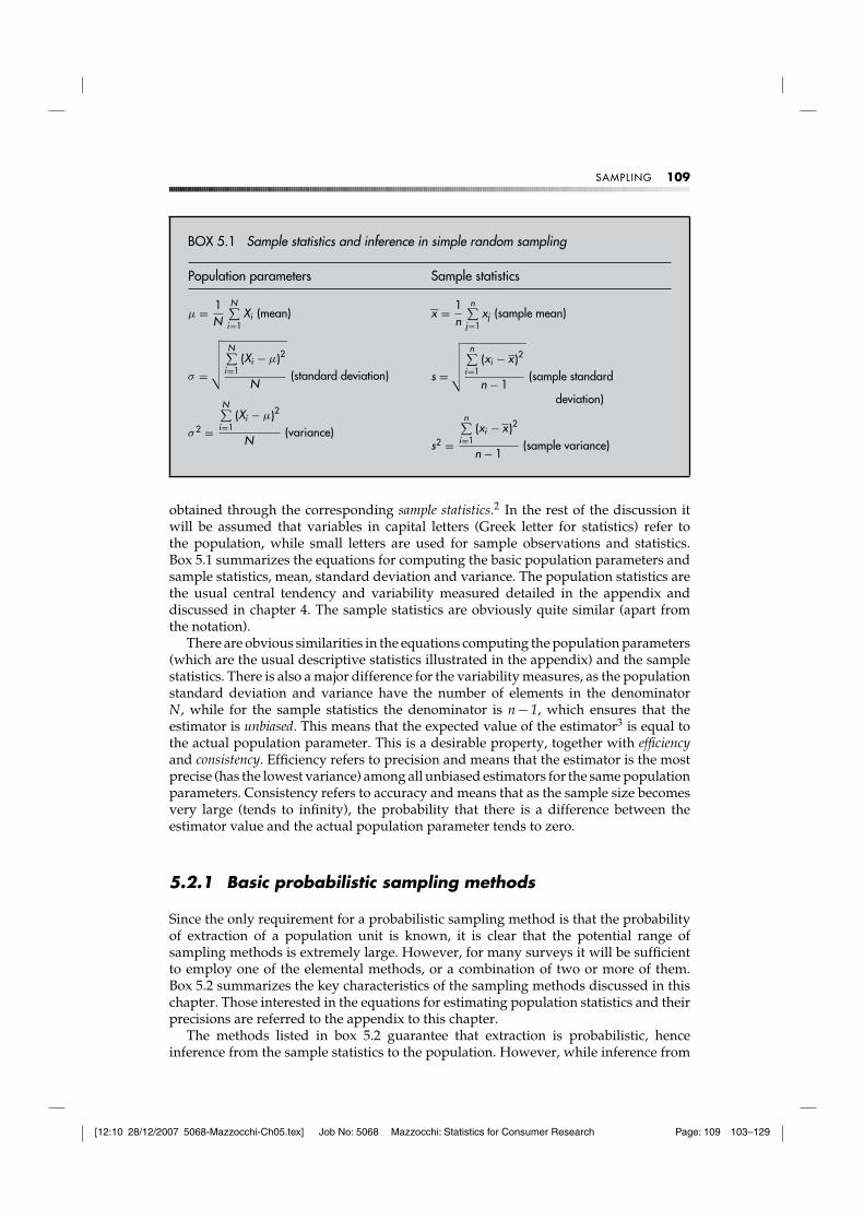
BOX 5.1 Sample statistics and inference in simple random sampling
Population parameters Sample statistics
µ = 1N
N∑i=1
Xi (mean)
σ =
√√√√√N∑
i=1(Xi − µ)2
N(standard deviation)
σ 2 =
N∑i=1
(Xi − µ)2
N(variance)
�x = 1n
n∑j=1
xj (sample mean)
s =
√√√√√n∑
i=1(xi − x )2
n − 1(sample standard
deviation)
s2 =
n∑i=1
(xi − x )2
n − 1(sample variance)
obtained through the corresponding sample statistics.2 In the rest of the discussion itwill be assumed that variables in capital letters (Greek letter for statistics) refer tothe population, while small letters are used for sample observations and statistics.Box 5.1 summarizes the equations for computing the basic population parameters andsample statistics, mean, standard deviation and variance. The population statistics arethe usual central tendency and variability measured detailed in the appendix anddiscussed in chapter 4. The sample statistics are obviously quite similar (apart fromthe notation).
There are obvious similarities in the equations computing the population parameters(which are the usual descriptive statistics illustrated in the appendix) and the samplestatistics. There is also a major difference for the variability measures, as the populationstandard deviation and variance have the number of elements in the denominatorN, while for the sample statistics the denominator is n − 1, which ensures that theestimator is unbiased. This means that the expected value of the estimator3 is equal tothe actual population parameter. This is a desirable property, together with efficiencyand consistency. Efficiency refers to precision and means that the estimator is the mostprecise (has the lowest variance) among all unbiased estimators for the same populationparameters. Consistency refers to accuracy and means that as the sample size becomesvery large (tends to infinity), the probability that there is a difference between theestimator value and the actual population parameter tends to zero.
5.2.1 Basic probabilistic sampling methods
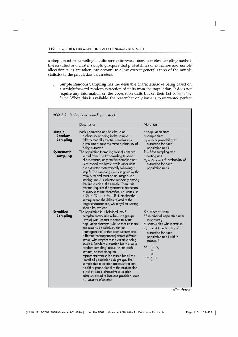
Since the only requirement for a probabilistic sampling method is that the probabilityof extraction of a population unit is known, it is clear that the potential range ofsampling methods is extremely large. However, for many surveys it will be sufficientto employ one of the elemental methods, or a combination of two or more of them.Box 5.2 summarizes the key characteristics of the sampling methods discussed in thischapter. Those interested in the equations for estimating population statistics and theirprecisions are referred to the appendix to this chapter.
The methods listed in box 5.2 guarantee that extraction is probabilistic, henceinference from the sample statistics to the population. However, while inference from
[12:10 28/12/2007 5068-Mazzocchi-Ch05.tex] Job No: 5068 Mazzocchi: Statistics for Consumer Research Page: 110 103–129
110 STATISTICS FOR MARKETING AND CONSUMER RESEARCH
a simple random sampling is quite straightforward, more complex sampling methodlike stratified and cluster sampling require that probabilities of extraction and sampleallocation rules are taken into account to allow correct generalization of the samplestatistics to the population parameters.
1. Simple Random Sampling has the desirable characteristic of being based ona straightforward random extraction of units from the population. It does notrequire any information on the population units but on their list or samplingframe. When this is available, the researcher only issue is to guarantee perfect
BOX 5.2 Probabilistic sampling methods
Description Notation
SimpleRandomSampling
Each population unit has the sameprobability of being in the sample. Itfollows that all potential samples of agiven size n have the same probability ofbeing extracted.
N population size;n sample size;π i = n/N probability of
extraction for eachpopulation unit i
Systematicsampling
The population (sampling frame) units aresorted from 1 to N according to somecharacteristic, only the first sampling unitis extracted randomly, while other unitsare extracted systematically following astep k . The sampling step k is given by theratio N/n and must be an integer. Thestarting unit r is selected randomly amongthe first k unit of the sample. Then, thismethod requires the systematic extractionof every k-th unit thereafter, i.e. units r+k,r+2k, r+3k, …, r+(n−1)k. Note that thesorting order should be related to thetarget characteristic, while cyclical sortingshould be avoided.
k = N/n sampling stepr starting unitπ i = n/N = 1/k probability of
extraction for eachpopulation unit i
StratifiedSampling
The population is subdivided into Scomplementary and exhaustive groups(strata) with respect to some relevantpopulation characteristic, so that units areexpected to be relatively similar(homogeneous) within each stratum anddifferent (heterogeneous) across differentstrata, with respect to the variable beingstudied. Random extraction (as in simplerandom sampling) occurs within eachstratum, so that adequaterepresentativeness is ensured for all theidentified population sub-groups. Thesample size allocation across strata canbe either proportional to the stratum sizeor follow some alternative allocationcriterion aimed to increase precision, suchas Neyman allocation
S number of strataNj number of population units
in stratum jnj sample size within stratum jπ ij = nj/Nj probability of
extraction for eachpopulation unit i withinstratum j
N =S∑
j=1Nj
n =S∑
j=1nj
(Continued)
[12:10 28/12/2007 5068-Mazzocchi-Ch05.tex] Job No: 5068 Mazzocchi: Statistics for Consumer Research Page: 111 103–129
SAMPLING 111
BOX 5.2 Cont’d
Description Notation
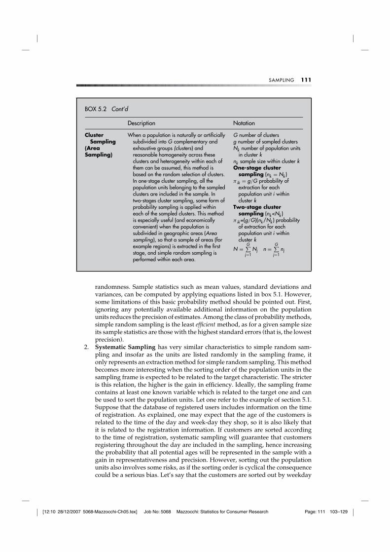
ClusterSampling
(AreaSampling)
When a population is naturally or artificiallysubdivided into G complementary andexhaustive groups (clusters) andreasonable homogeneity across theseclusters and heterogeneity within each ofthem can be assumed, this method isbased on the random selection of clusters.In one-stage cluster sampling, all thepopulation units belonging to the sampledclusters are included in the sample. Intwo-stages cluster sampling, some form ofprobability sampling is applied withineach of the sampled clusters. This methodis especially useful (and economicallyconvenient) when the population issubdivided in geographic areas (Areasampling), so that a sample of areas (forexample regions) is extracted in the firststage, and simple random sampling isperformed within each area.
G number of clustersg number of sampled clustersNk number of population units
in cluster knk sample size within cluster kOne-stage cluster
sampling (nk = Nk )π ik = g/G probability of
extraction for eachpopulation unit i withincluster k
Two-stage clustersampling (nk <Nk )
π ik =(g/G)(nk /Nk ) probabilityof extraction for eachpopulation unit i withincluster k
N =G∑
j=1Nj n =
G∑j=1
nj
randomness. Sample statistics such as mean values, standard deviations andvariances, can be computed by applying equations listed in box 5.1. However,some limitations of this basic probability method should be pointed out. First,ignoring any potentially available additional information on the populationunits reduces the precision of estimates. Among the class of probability methods,simple random sampling is the least efficient method, as for a given sample sizeits sample statistics are those with the highest standard errors (that is, the lowestprecision).
2. Systematic Sampling has very similar characteristics to simple random sam-pling and insofar as the units are listed randomly in the sampling frame, itonly represents an extraction method for simple random sampling. This methodbecomes more interesting when the sorting order of the population units in thesampling frame is expected to be related to the target characteristic. The stricteris this relation, the higher is the gain in efficiency. Ideally, the sampling framecontains at least one known variable which is related to the target one and canbe used to sort the population units. Let one refer to the example of section 5.1.Suppose that the database of registered users includes information on the timeof registration. As explained, one may expect that the age of the customers isrelated to the time of the day and week-day they shop, so it is also likely thatit is related to the registration information. If customers are sorted accordingto the time of registration, systematic sampling will guarantee that customersregistering throughout the day are included in the sampling, hence increasingthe probability that all potential ages will be represented in the sample with again in representativeness and precision. However, sorting out the populationunits also involves some risks, as if the sorting order is cyclical the consequencecould be a serious bias. Let’s say that the customers are sorted out by weekday
[12:10 28/12/2007 5068-Mazzocchi-Ch05.tex] Job No: 5068 Mazzocchi: Statistics for Consumer Research Page: 112 103–129
112 STATISTICS FOR MARKETING AND CONSUMER RESEARCH
and time of registration, so that the sampling frame starts with customersregistering on a Monday morning, then goes on with other Monday’s registrantsuntil the evening, then switches to Tuesday morning customers and so on. Aninappropriate sampling step could lead to the inclusion in the sample of allmorning registrants jumping all those who registered in afternoons or evenings.Clearly if the assumption that age is correlated to the time of registration istrue, the application of systematic sampling would lead to the extraction of aseriously biased sample. In synthesis, systematic sampling should be preferredto simple random sampling when a sorting variable related to the target variableis available, taking care to avoid any circuity in the sorting strategy.
A desirable feature of systematic sampling is that it can also be used withoutrequiring a sampling frame, or more precisely, the sampling frame is built whiledoing systematic sampling. For example, this is the case when only one in everyten customers at a supermarket till is stopped for interview. The sample is builtwithout knowing the list of customers on that day and the actual population sizeN is known only when the sampling process is terminated.
3. Stratified sampling is potentially the most efficient among elemental samplingstrategies. When the population can be easily divided into sub-groups (strata),random selection of sampling units within each of the sub-groups can lead tomajor gains in precision. The rationale behind this sampling process is thatthe target characteristics shows less variability within each stratum, as it isrelated to the stratification variable(s) and varies with it. Thus, by extracting thesample units from different strata, representativeness is increased. It is essentialto distinguish stratified sampling from the non-probability quota samplingdiscussed in the example of section 5.1 and in section 5.4. Stratified samplingrequires the actual subdivision of the sampling frame into subpopulations,so that random extraction is ensured independently within each of the strata.While this leads to an increase in costs it safeguards inference. Instead, quotasampling does not require any sampling frame and only presumes knowledgeof the proportional allocation of the sub-populations. Even with a random quotasampling, the sampling units are extracted from the overall population subjectto the rule to maintain the prescribed percentages of units coming from theidentified sub-populations. Referring to the example, in order to implement astratified sampling design, the researcher should:
(1) associate the (average) amount spent to each of the customers in thedatabase;
(2) sub-divide the sampling frame into two sub-groups, one with thosecustomers who spend more than £ 50, the other with those than spend less;
(3) decide on the size of each of the strata (for example 70 light shoppers and30 heavy shoppers if the population proportions are maintained);
(4) extract randomly and independently from the two sub-populations; and(5) compute the sample mean through a weighted average.
Besides increasing representativeness, stratified random sampling is particularlyuseful if separate estimates are needed for each sub-domain, for instanceestimating the average on-line shopper age separately for heavy and lightshoppers.
4. Cluster sampling is one of the most employed elemental methods and is oftena component of more complex methods. Its most desirable feature is that it doesnot necessarily require a list of population units, and it is hence applicable with
[12:10 28/12/2007 5068-Mazzocchi-Ch05.tex] Job No: 5068 Mazzocchi: Statistics for Consumer Research Page: 113 103–129
SAMPLING 113
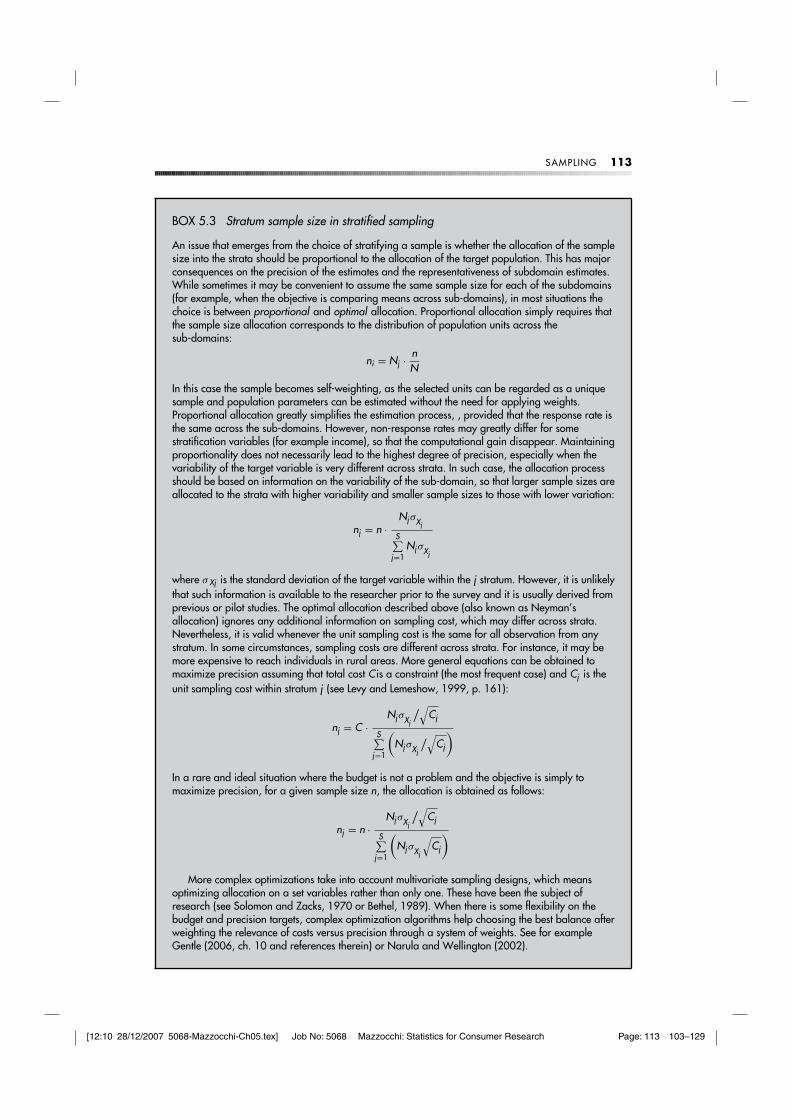
BOX 5.3 Stratum sample size in stratified sampling
An issue that emerges from the choice of stratifying a sample is whether the allocation of the samplesize into the strata should be proportional to the allocation of the target population. This has majorconsequences on the precision of the estimates and the representativeness of subdomain estimates.While sometimes it may be convenient to assume the same sample size for each of the subdomains(for example, when the objective is comparing means across sub-domains), in most situations thechoice is between proportional and optimal allocation. Proportional allocation simply requires thatthe sample size allocation corresponds to the distribution of population units across thesub-domains:
ni = Nj · nN
In this case the sample becomes self-weighting, as the selected units can be regarded as a uniquesample and population parameters can be estimated without the need for applying weights.Proportional allocation greatly simplifies the estimation process, , provided that the response rate isthe same across the sub-domains. However, non-response rates may greatly differ for somestratification variables (for example income), so that the computational gain disappear. Maintainingproportionality does not necessarily lead to the highest degree of precision, especially when thevariability of the target variable is very different across strata. In such case, the allocation processshould be based on information on the variability of the sub-domain, so that larger sample sizes areallocated to the strata with higher variability and smaller sample sizes to those with lower variation:
nj = n ·NjσXj
S∑j=1
NjσXj
where σ Xj is the standard deviation of the target variable within the j stratum. However, it is unlikelythat such information is available to the researcher prior to the survey and it is usually derived fromprevious or pilot studies. The optimal allocation described above (also known as Neyman’sallocation) ignores any additional information on sampling cost, which may differ across strata.Nevertheless, it is valid whenever the unit sampling cost is the same for all observation from anystratum. In some circumstances, sampling costs are different across strata. For instance, it may bemore expensive to reach individuals in rural areas. More general equations can be obtained tomaximize precision assuming that total cost C is a constraint (the most frequent case) and Cj is theunit sampling cost within stratum j (see Levy and Lemeshow, 1999, p. 161):
nj = C ·NjσXj
/√Cj
S∑j=1
(NjσXj
/√Cj
)
In a rare and ideal situation where the budget is not a problem and the objective is simply tomaximize precision, for a given sample size n, the allocation is obtained as follows:
nj = n ·NjσXj
/√Cj
S∑j=1
(NjσXj
√Cj
)
More complex optimizations take into account multivariate sampling designs, which meansoptimizing allocation on a set variables rather than only one. These have been the subject ofresearch (see Solomon and Zacks, 1970 or Bethel, 1989). When there is some flexibility on thebudget and precision targets, complex optimization algorithms help choosing the best balance afterweighting the relevance of costs versus precision through a system of weights. See for exampleGentle (2006, ch. 10 and references therein) or Narula and Wellington (2002).
[12:10 28/12/2007 5068-Mazzocchi-Ch05.tex] Job No: 5068 Mazzocchi: Statistics for Consumer Research Page: 114 103–129
114 STATISTICS FOR MARKETING AND CONSUMER RESEARCH
more convenient survey methods (as mall intercepts) and to geographical (area)sampling. In many situations, while it is impossible or economically unfeasibleto obtain a list of each individual sampling unit, it is relatively easy to definegroups (clusters) of sampling units.
To avoid confusion with stratified sampling, it is useful to establish themain difference between the two strategies. While stratified sampling aims tomaximize homogeneity within each stratum, cluster sampling is most effectivewhen heterogeneity within each cluster is high and the clusters are relativelysimilar.
As an example, consider a survey targeted to measure some characteristics ofcinema audience for a specific movie shown in London. A priori, it is not possibleto distinguish between those that will go and see that specific film. However,the researcher has information on the list of cinemas that will show the movie.A simple random sampling extraction can be carried out from the list to select asmall number of cinemas, then an exhaustive survey of the audience on a givenweek can be carried out. Cluster sampling can be articulated in more stages. Forinstance, if the above study had to be targeted on the whole UK population, in afirst stage a number of cities could be extracted and in a second stage a numberof cinemas could be extracted within each city.
While the feasibility and convenience of this method is obvious, the resultsare not necessarily satisfactory in terms of precision. Cluster sampling producerelatively large standard errors especially when the sampling units within eachcluster are homogeneous with respect to some characteristic. For example, givendifferences in ticket prices and cinema locations around the city, it is likely thatthe audience is relatively homogeneous in terms of socio-economic status. Thishas two consequences – first, it is necessary that the number of selected clustersis high enough to avoid a selection bias and secondly if there is low variabilitywithin a cluster, an exhaustive sampling (interviewing the whole audience) islikely to be excessive and unnecessarily expensive. Hence, the trade-off to beconsidered is between the benefits from limiting the survey to a small numberof clusters and the additional costs due to the excessive sampling rate. In caseswhere a sampling frame can actually be obtained for the selected clusters, aconvenient strategy is to apply simple random sampling or systematic samplingwithin the clusters.
5.2.2 Precision and accuracy of estimators
Given the many sampling options discussed in the previous sections, researchersneed to face many alternative choices, not to mention the frequent use of mixedand complex methods, as discussed later. In most case, the decision is made easy bybudget constraints. There are many trade-offs to be considered. For instance, randomsampling is the least efficient method among the probability ones, as it requires a largersample size to achieve the same precisions level of , say, stratified sampling. However,stratification is a costly process in itself, as the population units need to be classifiedaccording to the stratification variable.
As mentioned, efficiency is measured through the standard error, as shown in theappendix. In general, the standard error increases with higher population variances anddecreases with higher sample sizes. However, as sample size increases the relative gainin efficiency becomes smaller. This has some interesting and not intuitive implications.
[12:10 28/12/2007 5068-Mazzocchi-Ch05.tex] Job No: 5068 Mazzocchi: Statistics for Consumer Research Page: 115 103–129
SAMPLING 115
As shown below, it is not convenient to go above a certain sample size, because whilethe precision gain decreases the additional cost does not.
Standard error also increases with population size. However, the required samplingsize to attain a given level of precision does not increase proportionally with populationsize. Hence, as shown in the example of box 5.4, the target sample size does not varymuch between a relatively small population and a very large one.
A concept that might be useful when assessing the performance of estimators isrelative sampling accuracy (or relative sampling error), that is a measure of accuracy forthe estimated mean (or proportion) at a given level of confidence. If one considerssimple random sampling, relative accuracy can be computed by assuming a normaldistribution for the mean estimate. The confidence level α (further discussed in chapter6) is the probability that the relative difference between the estimated sample mean andthe population mean is larger than the relative accuracy level r:
Pr
(∣∣∣∣∣x − �X�X
∣∣∣∣∣ < r
)= 1 − α
where �X is the population mean and 1−α is the level of confidence.4 The aboveequation means that the probability that the difference between the sample mean andthe population mean (in percentage terms) is smaller than the fixed threshold r is equalto the level of confidence. Higher levels of confidence (lower levels of α) imply lessaccuracy (a higher r), which means that there is a trade-off between the confidencelevel and the target accuracy level. Thus one first fixes α at a relatively small level,usually at 0.05 or 0.01, which means a confidence level of 95% or 99%, respectively.Then it becomes possible to determine the relative accuracy level ras a function of thepopulation and sample size of the standard error and to a coefficient which dependson the value chosen for α.
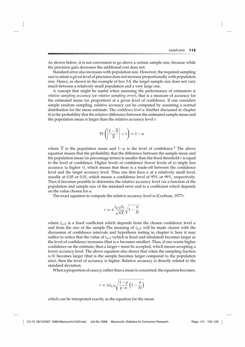
The exact equation to compute the relative accuracy level is (Cochran, 1977):
r = ± tα/2Sx√n�X
√1 − n
N
where tα/2 is a fixed coefficient which depends from the chosen confidence level α
and from the size of the sample.The meaning of tα/2 will be made clearer with thediscussion of confidence intervals and hypothesis testing in chapter 6; here it maysuffice to notice that the value of tα/2 (which is fixed and tabulated) becomes larger asthe level of confidence increases (that is α becomes smaller). Thus, if one wants higherconfidence on the estimate, then a larger r must be accepted, which means accepting alower accuracy level. The above equation also shows that when the sampling fractionn/N becomes larger (that is the sample becomes larger compared to the populationsize), then the level of accuracy is higher. Relative accuracy is directly related to thestandard deviation.
When a proportion of cases p, rather than a mean is concerned, the equation becomes.
r = ±tα/2
√1 − pp · n
(1 − n
N
)
which can be interpreted exactly as the equation for the mean.
[12:10 28/12/2007 5068-Mazzocchi-Ch05.tex] Job No: 5068 Mazzocchi: Statistics for Consumer Research Page: 116 103–129
116 STATISTICS FOR MARKETING AND CONSUMER RESEARCH
5.2.3 Deciding the sample size
When it is not a straightforward consequence of budget constraints, sample size isdetermined by several factors. It may depend on the precision level, especially whenthe research findings are expected to influence major decisions and there is little errortolerance. While box 5.4 shows that a size of 500 could do for almost any populationsize, another driving factor is the need for statistics on sub-groups of the population,which leads to an increase in the overall sample size. Also, if the survey topic isliable to be affected by non-response issues, it might be advisable to have a largerinitial sample size, although non-response should be treated with care as discussed inchapters 3 and 4. Sometimes, the real constraint is time. Some sampling strategies can beimplemented quickly, other are less immediate, especially when it becomes necessaryto add information to the sampling frame.
Since the precision of estimators depends on the sampling design, the determinationof sample size also requires different equations according to the chosen samplingmethod. Furthermore, since the sampling accuracy is based on a probability designand distributional assumption, it is necessary to set confidence levels, (introduced in
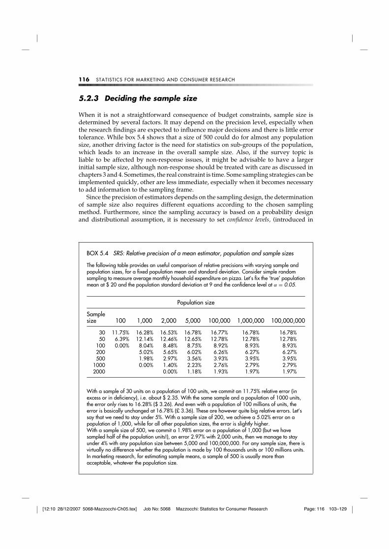
BOX 5.4 SRS: Relative precision of a mean estimator, population and sample sizes
The following table provides an useful comparison of relative precisions with varying sample andpopulation sizes, for a fixed population mean and standard deviation. Consider simple randomsampling to measure average monthly household expenditure on pizza. Let’s fix the ‘true’ populationmean at $ 20 and the population standard deviation at 9 and the confidence level at α = 0.05.
Population size
Samplesize 100 1,000 2,000 5,000 100,000 1,000,000 100,000,000
30 11.75% 16.28% 16.53% 16.78% 16.77% 16.78% 16.78%50 6.39% 12.14% 12.46% 12.65% 12.78% 12.78% 12.78%
100 0.00% 8.04% 8.48% 8.75% 8.92% 8.93% 8.93%200 5.02% 5.65% 6.02% 6.26% 6.27% 6.27%500 1.98% 2.97% 3.56% 3.93% 3.95% 3.95%
1000 0.00% 1.40% 2.23% 2.76% 2.79% 2.79%2000 0.00% 1.18% 1.93% 1.97% 1.97%
With a sample of 30 units on a population of 100 units, we commit an 11.75% relative error (inexcess or in deficiency), i.e. about $ 2.35. With the same sample and a population of 1000 units,the error only rises to 16.28% ($ 3.26). And even with a population of 100 millions of units, theerror is basically unchanged at 16.78% (£ 3.36). These are however quite big relative errors. Let’ssay that we need to stay under 5%. With a sample size of 200, we achieve a 5.02% error on apopulation of 1,000, while for all other population sizes, the error is slightly higher.With a sample size of 500, we commit a 1.98% error on a population of 1,000 (but we havesampled half of the population units!), an error 2.97% with 2,000 units, then we manage to stayunder 4% with any population size between 5,000 and 100,000,000. For any sample size, there isvirtually no difference whether the population is made by 100 thousands units or 100 millions units.In marketing research, for estimating sample means, a sample of 500 is usually more thanacceptable, whatever the population size.
[12:10 28/12/2007 5068-Mazzocchi-Ch05.tex] Job No: 5068 Mazzocchi: Statistics for Consumer Research Page: 117 103–129
SAMPLING 117
previous section and further explained in section 6.1), which should not be confusedwith precision measures. The latter can be controlled scientifically on the basis of themethod and the assumptions. But a high level of precision does not rule out verybad luck, as extracting samples randomly allows (with a lower probability) for extremesamples which provide inaccurate statistics. The confidence level specifies the risk levelthat the researcher is willing to take, as it is the probability value associated with aconfidence interval, which is the range of values which will include the population valuewith a probability equal to the confidence level (see chapter 6). Clearly, the width ofthe confidence interval and the confidence level are positively related. If one wantsa very precise estimate (a small confidence interval), the lower is the probability tofind the true population value within that bracket (a lower confidence). In order to getprecise estimates with a high confidence level, it is necessary to increase sample size.As discussed for accuracy, the confidence level is a probability measure which rangesbetween 0 and 1, usually denoted with (1−α), where α is the significance level, commonlyfixed to 0.05, which means confidence level of 0.95 (or 95%), or to 0.01 (99%) when riskaversion towards errors is higher.
Another non-trivial issue faced when determining the sample size is the knowledgeof one or more population parameters, generally the population variance. It is veryunlikely that such value is known beforehand, unless measured in previous studies.The common practice is to get some preliminary estimates through a pilot study,through a mathematical model (see for example Deming, 1990, ch. 14) or even makesome arbitrary (and conservative) assumption. Note that even in the situation wherethe population variance is underestimated (and hence the sample size is lower thanrequired), the sample statistics will still be unbiased although less efficient thanexpected.
In synthesis, the target sample size increases with the desired accuracy level andis higher for larger population variances and for higher confidence levels. In simplerandom sampling, the equation to determine the sample size for a given level ofaccuracy is the following:
n =(
tα/2σ
rµ
)2
As before, tα/2 is a fixed value (the tstatistic) which depends on the chosen confidencelevel 1−α. If the size is larger than 50, the fixed value tα/2can be replaced with theone taken from normal approximation (zα/2), σ is the known standard deviation of thepopulation (usually substituted by an estimate s), ris the relative accuracy level definedabove and µ is the population mean. Since the latter is also usually unknown (very likely,since most of the time it is the objective of the survey), it is also estimated through apilot study or a conservative guess can be used.
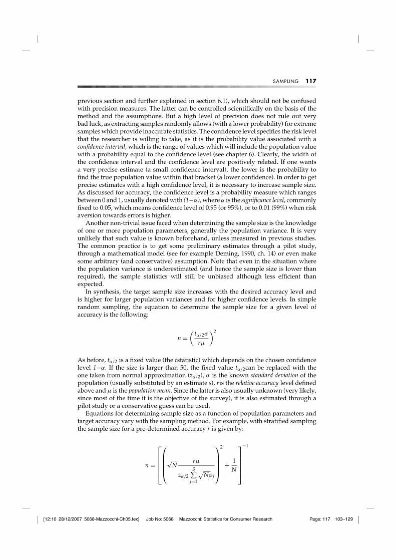
Equations for determining sample size as a function of population parameters andtarget accuracy vary with the sampling method. For example, with stratified samplingthe sample size for a pre-determined accuracy r is given by:
n =
⎡⎢⎢⎢⎢⎣
⎛⎜⎜⎜⎜⎝
√N
rµ
zα/2S∑
j=1
√Njsj
⎞⎟⎟⎟⎟⎠
2
+ 1N
⎤⎥⎥⎥⎥⎦
−1
[12:10 28/12/2007 5068-Mazzocchi-Ch05.tex] Job No: 5068 Mazzocchi: Statistics for Consumer Research Page: 118 103–129
118 STATISTICS FOR MARKETING AND CONSUMER RESEARCH
5.2.4 Post-stratification
A typical obstacle to the implementation of stratified sampling is the unavailability ofa sampling frame for each of the identified strata, which implies the knowledge of thestratification variable(s) for all the population units. In such a circumstance it may beuseful to proceed through simple random sampling and exploit the stratified estimatoronce the sample has been extracted, which increases efficiency. All that is required isthe knowledge of the stratum sizes in the population and that such post-stratum sizesare sufficiently large. The advantage of post-stratifications is two-fold:
• It allows to correct the potential bias due to insufficient coverage of the survey(incomplete sampling frame); and
• It allows to correct the bias due to missing responses, provided that the post-stratification variable is related both to the target variable and to the cause ofnon-response
Post-stratification is carried out by extracting a simple random sample of size n, andthen units are classified into strata. Instead of the usual SRS mean, a post-stratifiedestimator is computed by weighting the means of the sub-groups by the size of eachsub-group. The procedure is identical to the one of stratified sampling and the onlydifference is that the allocation into strata is made ex-post. The gain in precision isrelated to the sample size in each stratum and (inversely) to the difference betweenthe sample weights and the population ones (the complex equation for the unbiasedestimator for the standard error of the mean is provided in the appendix to this chapter).The standard error for the post-stratified mean estimator is larger than the stratifiedsampling one, because additional variability is given by the fact that the sample stratumsizes are themselves the outcome of a random process.
5.2.5 Sampling solutions to non-sampling errors
A review of the non-sampling sources of errors is provided in chapter 3, but it may beuseful to discuss here some methods to reduce the biases of an actual sample which issmaller than the planned one or less representative than expected. This is generally dueto two sources of errors – non-response errors, when some of the sampling units cannotbe reached, are unable or unwilling to answer to the survey questions and incompletesampling frames, when the sampling frame does not fully cover the target population(coverage error). In estimating a sample mean, the size of these errors is
(a) directly proportional to the discrepancy between the mean value for the actuallysampled units and the (usually unknown) mean value for those units that couldnot be sampled and
(b) inversely proportional to the proportion of non-respondents on the total sample(or to the proportion of those that are not included the sampling frame on thetotal population size).
The post-stratification method is one solution to non-response errors, especiallyuseful when a specific stratum is under-represented in the sample. For example, atelephone survey might be biased by an under-representation of those people whospend less time at home, like commuters and those who often travel for work as
[12:10 28/12/2007 5068-Mazzocchi-Ch05.tex] Job No: 5068 Mazzocchi: Statistics for Consumer Research Page: 119 103–129
SAMPLING 119
compared to pensioners and housewives. The relevance of this bias can be highif this characteristic is related to the target variable. Still considering the exampleof box 5.5, if the target variable is the level of satisfaction with railways, thisgroup is likely to be very important. If the proportion of commuters on the targetpopulation is known (or estimated in a separate survey), post-stratification constitutesa non-response correction as it gives the appropriate weight to the under-representedsubgroup.
Similarly, post-stratification may help in situations where the problem lies in thesampling frame. If the phone book is used as a sampling frame, household in somerural areas where not all households have a phone line will be under-represented.Another solution is the use of dual frame surveys, specifically two parallel samplingframes (for example white pages and electoral register) and consequently two differentsurvey methods (personal interviews for those sampled through the electoral register).Other methods (see Thompson, 1997) consist in extracting a further random sampleout of the list of non-respondents (to get representative estimates for the group ofnon-respondents), in using a regression estimator or a ratio estimator or in weightingsample units through same demographic or socio-economic variables measured inthe population. This latter method is similar to post-stratification, but not identicalas unlike post-stratification it does not require homogeneity within each stratum andheterogeneity across strata.
5.2.6 Complex probabilistic sampling methods
The probability methods discussed in this chapter can be combined and developedinto more complex sampling strategies, aimed at increasing efficiency or reducing costthrough more practical targeting.
A commonly used approach in sampling household is two-stage sampling. Most ofthe household budget surveys in Europe are based on this method. Two-stage methodsimply the use of two different sampling units, where the second-stage sampling unitsare a sub-set of the first-stage ones. Typically, a sample of cities or municipalities isextracted in the first stage, while in the second stage the actual sample of householdsis extracted out of the first-stage units. Any probability design can be applied withineach stage. For example, municipalities can be stratified according to their populationsin the first stage, to ensure that the sample will include small and rural towns as well aslarge cities, while in the second stage one could apply area sampling, a particular typeof cluster sampling where:
(1) each sampled municipality is subdivided into blocks on a map throughgeographical co-ordinates;
(2) blocks are extracted through simple random sampling; and(3) all households in a block are interviewed.
Clearly, if the survey method is personal interview, this sampling strategy min-imizes costs as the interviewers will be able to cover many sampling units in asmall area.
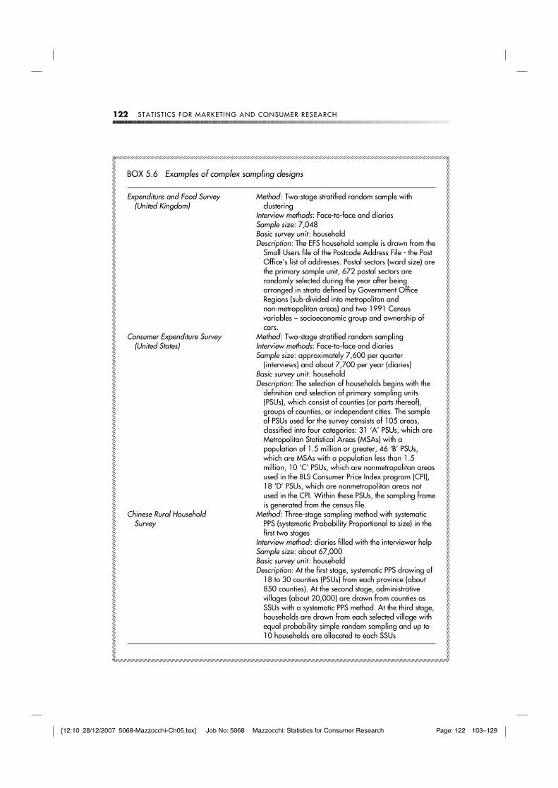
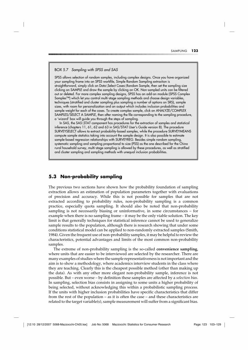
As complex methods are subject to a number of adjustments and options, the samplestatistics can become very complex themselves. Box 5.6 below brings real examples ofcomplex sampling design in consumer research, while box 5.7 illustrates how samplescan be extracted from sampling frames in SPSS and SAS.
[12:10 28/12/2007 5068-Mazzocchi-Ch05.tex] Job No: 5068 Mazzocchi: Statistics for Consumer Research Page: 120 103–129
120 STATISTICS FOR MARKETING AND CONSUMER RESEARCH
≈≈≈≈≈≈≈≈≈≈≈≈≈≈≈≈≈≈≈≈≈≈≈≈≈≈≈≈≈≈≈≈≈≈≈≈≈≈≈≈≈≈≈≈≈≈≈≈≈≈≈≈≈≈≈≈≈≈≈≈≈≈≈≈≈≈≈≈≈≈≈≈≈≈≈≈≈≈≈≈≈≈≈≈
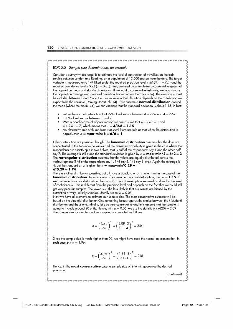
BOX 5.5 Sample size determination: an example
Consider a survey whose target is to estimate the level of satisfaction of travellers on the trainservice between London and Reading, on a population of 13,500 season ticket holders. The targetvariable is measured on a 1–7 Likert scale, the required precision level is ±10% (r = 0.1) and therequired confidence level is 95% (α = 0.05). First, we need an estimate (or a conservative guess) ofthe population mean and standard deviation. If we want a conservative estimate, we may choosethe population average and standard deviation that maximize the ratio (σ/µ). The average µ mustbe included between 1 and 7 and the maximum standard deviation depends on the distribution weexpect from the variable (Deming, 1990, ch. 14). If we assume a normal distribution aroundthe mean (where the mean is 4), we can estimate that the standard deviation is about 1.15, in fact:
• within the normal distribution that 99% of values are between 4 − 2.6σ and 4 + 2.6σ
• 100% of values are between 1 and 7• With a good degree of approximation we can assume that 4 − 2.6σ = 1 and
4 + 2.6σ = 7, which means that σ = 3/2.6 = 1.15• An alternative rule of thumb from statistical literature tells us that when the distribution is
normal, then σ = max–min/6 = 6/6 = 1
Other distribution are possible, though. The binomial distribution assumes that the data areconcentrated in the two extreme values and the maximum variability is given in the case where therespondents are exactly split in two halves, that is half of the respondents say 1 and the other halfsay 7. The average is still 4 and the standard deviation is given by σ = max–min/2 = 6/2 = 3The rectangular distribution assumes that the values are equally distributed across thevarious options (1/6 of the respondents say 1, 1/6 say 2, 1/6 say 3, etc.). Again the average is4, but the standard error is given by σ = max–min*0.29 =6*0.29 = 1.74There are other distribution possible, but all have a standard error smaller than in the case of thebinomial distribution. To summarize: if we assume a normal distribution, then σ = 1.15. Ifwe assume a binomial distribution, then σ = 3. The last assumption we need is related to the levelof confidence α. This is different from the precision level and depends on the fact that we could stillget very peculiar samples. The lower is α, the less likely is that our results are biased by theextraction of very unlikely samples. Usually we set α = 0.05.Now we have all elements to estimate our sample size. The most conservative estimate will bebased on the binomial distribution.One remaining issues regards the choice between the t (student)distribution and the z one. Initially, let’s be very conservative and let’s assume that the sample isgoing to include around 20 units. Hence, with α = 0.05, we use the statistic t0.025(20) = 2.09The sample size for simple random sampling is computed as follows:
n =(
tα/2σ
rµ
)2=(
2.09 · 30.1 · 4
)2= 246
Since the sample size is much higher than 50, we might have used the normal approximation. Insuch case z0.025 = 1.96:
n =(
zα/2σ
rµ
)2=(
1.96 · 30.1 · 4
)2= 216
Hence, in the most conservative case, a sample size of 216 will guarantee the desiredprecision.
(Continued)
≈≈≈≈
≈≈≈≈
≈≈≈≈
≈≈≈≈
≈≈≈≈
≈≈≈≈
≈≈≈≈
≈≈≈≈
≈≈≈≈
≈≈≈≈
≈≈≈≈
≈≈≈≈
≈≈≈≈
≈≈≈≈
≈≈≈≈
≈≈≈≈
≈≈≈≈
≈≈≈≈
≈≈≈≈
≈≈≈≈
≈≈≈≈
≈≈≈≈
≈≈≈≈
≈≈≈≈
≈≈≈≈
≈≈≈≈
≈≈≈≈
≈≈≈≈
≈≈≈≈
≈≈≈≈
≈≈≈≈
≈≈≈≈
≈≈≈≈
≈≈≈≈≈≈≈≈≈≈≈≈≈≈≈≈≈≈≈≈≈≈≈≈≈≈≈≈≈≈≈≈≈≈≈≈≈≈≈≈≈≈≈≈≈≈≈≈≈≈≈≈≈≈≈≈≈≈≈≈≈≈≈≈≈≈≈≈≈≈≈≈≈≈≈≈≈≈≈≈≈≈≈≈ ≈≈≈≈
≈≈≈≈
≈≈≈≈
≈≈≈≈
≈≈≈≈
≈≈≈≈
≈≈≈≈
≈≈≈≈
≈≈≈≈
≈≈≈≈
≈≈≈≈
≈≈≈≈
≈≈≈≈
≈≈≈≈
≈≈≈≈
≈≈≈≈
≈≈≈≈
≈≈≈≈
≈≈≈≈
≈≈≈≈
≈≈≈≈
≈≈≈≈
≈≈≈≈
≈≈≈≈
≈≈≈≈
≈≈≈≈
≈≈≈≈
≈≈≈≈
≈≈≈≈
≈≈≈≈
≈≈≈≈
≈≈≈≈
≈≈≈≈
[12:10 28/12/2007 5068-Mazzocchi-Ch05.tex] Job No: 5068 Mazzocchi: Statistics for Consumer Research Page: 121 103–129
SAMPLING 121
≈≈≈≈≈≈≈≈≈≈≈≈≈≈≈≈≈≈≈≈≈≈≈≈≈≈≈≈≈≈≈≈≈≈≈≈≈≈≈≈≈≈≈≈≈≈≈≈≈≈≈≈≈≈≈≈≈≈≈≈≈≈≈≈≈≈≈≈≈≈≈≈≈≈≈≈≈≈≈≈≈≈≈≈
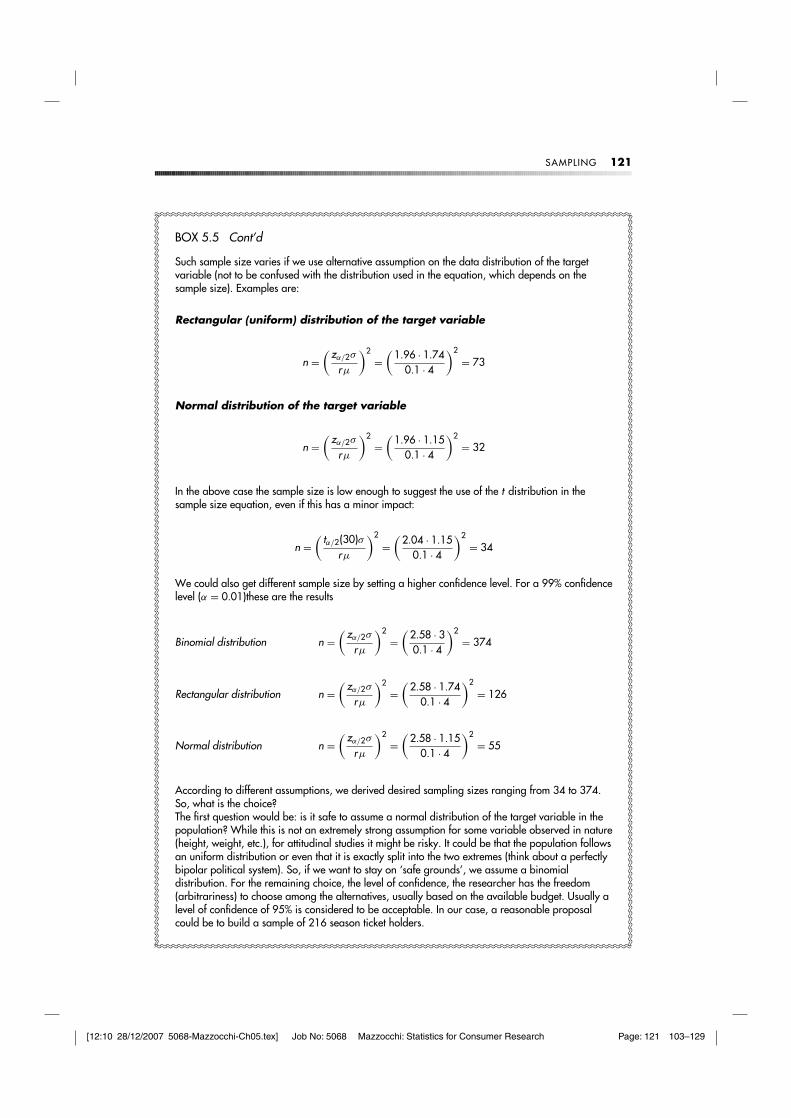
BOX 5.5 Cont’d
Such sample size varies if we use alternative assumption on the data distribution of the targetvariable (not to be confused with the distribution used in the equation, which depends on thesample size). Examples are:
Rectangular (uniform) distribution of the target variable
n =(
zα/2σ
rµ
)2=(
1.96 · 1.740.1 · 4
)2
= 73
Normal distribution of the target variable
n =(
zα/2σ
rµ
)2=(
1.96 · 1.150.1 · 4
)2= 32
In the above case the sample size is low enough to suggest the use of the t distribution in thesample size equation, even if this has a minor impact:
n =(
tα/2(30)σrµ
)2
=(
2.04 · 1.150.1 · 4
)2
= 34
We could also get different sample size by setting a higher confidence level. For a 99% confidencelevel (α = 0.01)these are the results
Binomial distribution n =(
zα/2σ
rµ
)2=(
2.58 · 30.1 · 4
)2= 374
Rectangular distribution n =(
zα/2σ
rµ
)2=(
2.58 · 1.740.1 · 4
)2
= 126
Normal distribution n =(
zα/2σ
rµ
)2=(
2.58 · 1.150.1 · 4
)2= 55
According to different assumptions, we derived desired sampling sizes ranging from 34 to 374.So, what is the choice?The first question would be: is it safe to assume a normal distribution of the target variable in thepopulation? While this is not an extremely strong assumption for some variable observed in nature(height, weight, etc.), for attitudinal studies it might be risky. It could be that the population followsan uniform distribution or even that it is exactly split into the two extremes (think about a perfectlybipolar political system). So, if we want to stay on ‘safe grounds’, we assume a binomialdistribution. For the remaining choice, the level of confidence, the researcher has the freedom(arbitrariness) to choose among the alternatives, usually based on the available budget. Usually alevel of confidence of 95% is considered to be acceptable. In our case, a reasonable proposalcould be to build a sample of 216 season ticket holders.
≈≈≈≈
≈≈≈≈
≈≈≈≈
≈≈≈≈
≈≈≈≈
≈≈≈≈
≈≈≈≈
≈≈≈≈
≈≈≈≈
≈≈≈≈
≈≈≈≈
≈≈≈≈
≈≈≈≈
≈≈≈≈
≈≈≈≈
≈≈≈≈
≈≈≈≈
≈≈≈≈
≈≈≈≈
≈≈≈≈
≈≈≈≈
≈≈≈≈
≈≈≈≈
≈≈≈≈
≈≈≈≈
≈≈≈≈
≈≈≈≈
≈≈≈≈
≈≈≈≈
≈≈≈≈
≈≈≈≈
≈≈≈≈
≈
≈≈≈≈≈≈≈≈≈≈≈≈≈≈≈≈≈≈≈≈≈≈≈≈≈≈≈≈≈≈≈≈≈≈≈≈≈≈≈≈≈≈≈≈≈≈≈≈≈≈≈≈≈≈≈≈≈≈≈≈≈≈≈≈≈≈≈≈≈≈≈≈≈≈≈≈≈≈≈≈≈≈≈≈ ≈≈≈≈
≈≈≈≈
≈≈≈≈
≈≈≈≈
≈≈≈≈
≈≈≈≈
≈≈≈≈
≈≈≈≈
≈≈≈≈
≈≈≈≈
≈≈≈≈
≈≈≈≈
≈≈≈≈
≈≈≈≈
≈≈≈≈
≈≈≈≈
≈≈≈≈
≈≈≈≈
≈≈≈≈
≈≈≈≈
≈≈≈≈
≈≈≈≈
≈≈≈≈
≈≈≈≈
≈≈≈≈
≈≈≈≈
≈≈≈≈
≈≈≈≈
≈≈≈≈
≈≈≈≈
≈≈≈≈
≈≈≈≈
≈
[12:10 28/12/2007 5068-Mazzocchi-Ch05.tex] Job No: 5068 Mazzocchi: Statistics for Consumer Research Page: 122 103–129
122 STATISTICS FOR MARKETING AND CONSUMER RESEARCH
≈≈≈≈≈≈≈≈≈≈≈≈≈≈≈≈≈≈≈≈≈≈≈≈≈≈≈≈≈≈≈≈≈≈≈≈≈≈≈≈≈≈≈≈≈≈≈≈≈≈≈≈≈≈≈≈≈≈≈≈≈≈≈≈≈≈≈≈≈≈≈≈≈≈≈≈≈≈≈≈≈≈≈≈
BOX 5.6 Examples of complex sampling designs
Expenditure and Food Survey(United Kingdom)
Method : Two-stage stratified random sample withclustering
Interview methods: Face-to-face and diariesSample size: 7,048Basic survey unit : householdDescription: The EFS household sample is drawn from the
Small Users file of the Postcode Address File - the PostOffice’s list of addresses. Postal sectors (ward size) arethe primary sample unit, 672 postal sectors arerandomly selected during the year after beingarranged in strata defined by Government OfficeRegions (sub-divided into metropolitan andnon-metropolitan areas) and two 1991 Censusvariables – socioeconomic group and ownership ofcars.
Consumer Expenditure Survey(United States)
Method : Two-stage stratified random samplingInterview methods: Face-to-face and diariesSample size: approximately 7,600 per quarter
(interviews) and about 7,700 per year (diaries)Basic survey unit : householdDescription: The selection of households begins with the
definition and selection of primary sampling units(PSUs), which consist of counties (or parts thereof),groups of counties, or independent cities. The sampleof PSUs used for the survey consists of 105 areas,classified into four categories: 31 ‘A’ PSUs, which areMetropolitan Statistical Areas (MSAs) with apopulation of 1.5 million or greater, 46 ‘B’ PSUs,which are MSAs with a population less than 1.5million, 10 ‘C’ PSUs, which are nonmetropolitan areasused in the BLS Consumer Price Index program (CPI),18 ‘D’ PSUs, which are nonmetropolitan areas notused in the CPI. Within these PSUs, the sampling frameis generated from the census file.
Chinese Rural HouseholdSurvey
Method : Three-stage sampling method with systematicPPS (systematic Probability Proportional to size) in thefirst two stages
Interview method : diaries filled with the interviewer helpSample size: about 67,000Basic survey unit : householdDescription: At the first stage, systematic PPS drawing of
18 to 30 counties (PSUs) from each province (about850 counties). At the second stage, administrativevillages (about 20,000) are drawn from counties asSSUs with a systematic PPS method. At the third stage,households are drawn from each selected village withequal probability simple random sampling and up to10 households are allocated to each SSUs
≈≈≈≈
≈≈≈≈
≈≈≈≈
≈≈≈≈
≈≈≈≈
≈≈≈≈
≈≈≈≈
≈≈≈≈
≈≈≈≈
≈≈≈≈
≈≈≈≈
≈≈≈≈
≈≈≈≈
≈≈≈≈
≈≈≈≈
≈≈≈≈
≈≈≈≈
≈≈≈≈
≈≈≈≈
≈≈≈≈
≈≈≈≈
≈≈≈≈
≈≈≈≈
≈≈≈≈
≈≈≈≈
≈≈≈≈
≈≈≈≈
≈≈≈≈
≈≈≈≈
≈≈≈≈
≈≈≈≈
≈≈
≈≈≈≈≈≈≈≈≈≈≈≈≈≈≈≈≈≈≈≈≈≈≈≈≈≈≈≈≈≈≈≈≈≈≈≈≈≈≈≈≈≈≈≈≈≈≈≈≈≈≈≈≈≈≈≈≈≈≈≈≈≈≈≈≈≈≈≈≈≈≈≈≈≈≈≈≈≈≈≈≈≈≈≈ ≈≈≈≈
≈≈≈≈
≈≈≈≈
≈≈≈≈
≈≈≈≈
≈≈≈≈
≈≈≈≈
≈≈≈≈
≈≈≈≈
≈≈≈≈
≈≈≈≈
≈≈≈≈
≈≈≈≈
≈≈≈≈
≈≈≈≈
≈≈≈≈
≈≈≈≈
≈≈≈≈
≈≈≈≈
≈≈≈≈
≈≈≈≈
≈≈≈≈
≈≈≈≈
≈≈≈≈
≈≈≈≈
≈≈≈≈
≈≈≈≈
≈≈≈≈
≈≈≈≈
≈≈≈≈
≈≈≈≈
≈≈
[12:10 28/12/2007 5068-Mazzocchi-Ch05.tex] Job No: 5068 Mazzocchi: Statistics for Consumer Research Page: 123 103–129
SAMPLING 123
BOX 5.7 Sampling with SPSS and SAS
SPSS allows selection of random samples, including complex designs. Once you have organizedyour sampling frame into an SPSS workfile, Simple Random Sampling extraction isstraightforward, simply click on Data\Select Cases\Random Sample, then set the sampling sizeclicking on SAMPLE and draw the sample by clicking on OK. Non-sampled units can be filteredout or deleted. For more complex sampling designs, SPSS has an add-on module (SPSS ComplexSamples™) which let you control multi-stage sampling methods and choose design variables,techniques (stratified and cluster sampling plus sampling a number of options on SRS), samplesizes, with room for personalization and an output which includes inclusion probabilities andsample weight for each of the cases. To create complex sample, click on ANALYZE/COMPLEXSAMPLES/SELECT A SAMPLE, then after naming the file corresponding to the sampling procedure,a ‘wizard’ box will guide you through the steps of sampling.
In SAS, the SAS\STAT component has procedures for the extraction of samples and statisticalinference (chapters 11, 61, 62 and 63 in SAS/STAT User’s Guide version 8). The procedureSURVEYSELECT allows to extract probability-based samples, while the procedure SURVEYMEANScompute sample statistics taking into account the sample design. It is also possible to estimatesample-based regression relationships with SURVEYREG. Besides simple random sampling,systematic sampling and sampling proportional to size (PSS) as the one described for the Chinarural household survey, multi-stage sampling is allowed by these procedures, as well as stratifiedand cluster sampling and sampling methods with unequal inclusion probabilities.
5.3 Non-probability sampling
The previous two sections have shown how the probability foundation of samplingextraction allows an estimation of population parameters together with evaluationsof precision and accuracy. While this is not possible for samples that are notextracted according to probability rules, non-probability sampling is a commonpractice, especially quota sampling. It should also be noted that non-probabilitysampling is not necessarily biasing or uninformative, in some circumstances – forexample when there is no sampling frame – it may be the only viable solution. The keylimit is that generally techniques for statistical inference cannot be used to generalizesample results to the population, although there is research showing that under someconditions statistical model can be applied to non-randomly extracted samples (Smith,1984). Given the frequent use of non-probability samples, it may be helpful to review thecharacteristics, potential advantages and limits of the most common non-probabilitysamples.
The extreme of non-probability sampling is the so-called convenience sampling,where units that are easier to be interviewed are selected by the researcher. There aremany examples of studies where the sample representativeness is not important and theaim is to show a methodology, where academics interview students in the class wherethey are teaching. Clearly this is the cheapest possible method (other than making upthe data). As with any other more elegant non-probability sample, inference is notpossible. But – even worse – by definition these samples are affected by a selection bias.In sampling, selection bias consists in assigning to some units a higher probability ofbeing selected, without acknowledging this within a probabilistic sampling process.If the units with higher inclusion probabilities have specific characteristics that differfrom the rest of the population – as it is often the case – and these characteristics arerelated to the target variable(s), sample measurement will suffer from a significant bias.
[12:10 28/12/2007 5068-Mazzocchi-Ch05.tex] Job No: 5068 Mazzocchi: Statistics for Consumer Research Page: 124 103–129
124 STATISTICS FOR MARKETING AND CONSUMER RESEARCH
There are many sources of selection bias and some depend on the interview methodrather than the sampling strategy. Consider this example of a selection bias due toconvenience sampling. A researcher wants to measure consumer willingness to pay fora fish meal and decides to interview people in fish restaurants, which will allow him toachieve easily a large sample size. While the researcher will be able to select many fishlovers, it is also true that the sample will miss all those people who like fish but considerexisting restaurant fish meals too expensive and prefer to cook it at home. The selectionbias will lead to a higher willingness to pay than the actual one. The sample cannotbe considered representative of consumers in general, but only of the set of selectedsample units.
Even if the researcher leaves behind convenience and tries to select units withoutany prior criteria, as in haphazard sampling, without a proper sampling frame and anextraction method based on probability inference is not valid.
In other circumstances, the use of a prior non-probability criterion for selection ofsample units is explicitly acknowledge. For example, in judgmental sampling, selectionis based on judgment of researchers who exploit their experience to draw a sample thatthey consider representative of the target population. The subjective element is nowapparent.
Quota sampling is possibly the most controversial (and certainly the most adopted) ofnon-probability technique. It is often mistaken for stratified sampling, but it generallydoes not guarantee the efficiency and representativeness of its counterpart. As shownin box 5.1, quota sampling does not follow probabilistic rules for extraction. Wherethere are one or more classification variables for which the percentage of populationunits is known, quota sampling only requires that the same proportions apply tothe sample. It is certainly cheaper than stratified sampling, given that only thesepercentages are required as compared to the need for a sampling frame for eachstratum. The main difference from judgmental sampling is that judgment is basedon the choice of variables defining quotas. Sampling error cannot be quantified inquota sampling and there is no way to assess sample representativeness. Furthermore,this sampling method is exposed to selection biases as extraction within each quotais still based on haphazard methods if not on convenience or judgment. There aresome relevant advantages in applying quota sampling, which may explain whyit is common practice for marketing research companies. Quota sampling is oftenimplemented in computer packages for CATI, CAPI and CAWI interviews (seechapter 3), where units are extracted randomly but retained in the sample only ifthey are within the quota. While this alters the probability design, it offers somecontrol on biases from non-response errors, since non-respondents are substitutedwith units from the same quota. The point in favour of quota sampling is that aprobability sample with a large portion of non-responses is likely to be worse thanquota sampling dealing with non-responses. Obviously, probability sampling withappropriate methods for dealing with non-responses as those mentioned in section5.2.5 are preferable.
If the objective of a research is to exploit a sample to draw conclusion on thepopulation or generalize the results, non-probability sampling methods are clearlyinadequate. For confirmatory studies where probability sampling is possible, non-probability methods should be always avoided. However, in many circumstances theyare accepted, especially when the aim of research is qualitative or simply preliminary toquantitative research (like piloting a questionnaire). Qualitative research is exploratoryrather than confirmatory and provides an unstructured and flexible understanding ofthe problem and its reliance on the basis of small samples. It can be a valuable toolwhen operating in contexts where a proper sampling process is unfeasible. A typical
[12:10 28/12/2007 5068-Mazzocchi-Ch05.tex] Job No: 5068 Mazzocchi: Statistics for Consumer Research Page: 125 103–129
SAMPLING 125
situation is when the target population is a very rare population, small and difficultto be singled out. In this circumstance, a useful non-probability technique is snowballsampling. As indicated by its name, snowball sampling starts with the selection of afirst small sample (possibly randomly). Then, to increase sample size, respondents areasked to identify others who belong to the population of interests, so that the referralshave demographic and psychographic characteristics similar to the referrers. Suppose,for example, that the objective is to interview those people who climbed Mount Everestin a given year (or, say, the readers of this book) and no records are available. Afterselecting a first small sample, it is very likely that those that have been selected will beable to indicate others who accomplished to the task.
Summing upSampling techniques allow one to estimate statistics on large target populationsby running a survey on a smaller sub-set of subjects. When subjects areextracted randomly to be included in a sample and the probabilities ofextraction are known, the sample is said to be probabilistic. The advantageof probability samples compared to those extracted through non-probabilityrules is the possibility of estimating the sampling error, which is the portionof error in the estimates which is due to the fact that only a sub-set of thepopulation is surveyed. This does not exhaust the total error committedby running a survey because non-sampling errors like non-response errorsalso need to be taken into account (see chapters 3 and 4). The basic formof probability sampling is simple random sampling, where all subjects inthe target population have the same probability of being inextracted. Otherforms of probability sampling include: systematic sampling, where subjectsare extracted at a systematic pace and cluster sampling, where the populationis first subdivided into cluster that are similar between each other and thena sub-set of cluster is extracted; stratified sampling, where the population isfirst subdivided into strata that contains homogeneous subjects but are quitedifferent from those in other strata. These techniques can be combined inmore complex sampling strategies, as in the multi-stage techniques adoptedfor official household budget survey. Once the sample has been extractedit is possible to generalize (infer) the sample characteristics like mean andvariance to the whole population by exploiting knowledge of the probabilitydistribution (see chapter 6). Estimates of the parameters are accompanied byestimates of their precision, as generally measured by the standard error.Accuracy (that is departure from the true population mean) can also beassessed with some degree of confidence. When planning a sample survey,there is a trade-off between sample size (cost) and precision. The latter alsodepends on the variability and dimension of the target population. Statisticalrules allows to determine the sample size depending on targeted accuracy andvice versa.
Non-probability samples, including the frequently employed quota sam-pling, are not based on statistical rules and depend on subjective and conve-nience choices. They can be useful in some circumstances where probabilitysampling is impossible or unnecessary, otherwise probability alternativesshould be chosen.
[12:10 28/12/2007 5068-Mazzocchi-Ch05.tex] Job No: 5068 Mazzocchi: Statistics for Consumer Research Page: 126 103–129
Ap
pen
dix
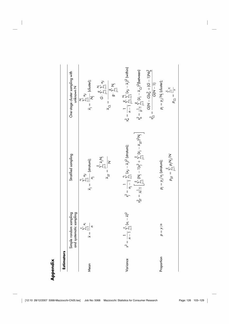
Esti
ma
tors
Sim
ple
rand
omsa
mpl
ing
and
syste
mat
icsa
mpl
ing
Stra
tified
sam
plin
gO
ne-s
tage
clus
ter
sam
plin
gw
ithun
know
nN
Mea
nx
=
n ∑ i=1
x i nx j
=
n j ∑ i=1
x ji
n j(s
tratu
m);
x ST=
S ∑ j=1
x jN
j
N
x j=
Nj ∑ i=1
x ji
Nj
(clu
ster)
;
x CL
=G
·g ∑ j=1
Nj ∑ i=1
x ji
g·g ∑ j=
1N
j
Var
ianc
es2
=1
n−
1
n ∑ i=1
(xi−
x)2
s2 j=
1n j
−1
n j ∑ i=1
(xji
−x j
)2(s
tratu
m);
s2 ST=
1N
−1
[ S ∑ j=1
(Nj−
1)s2 j
+S ∑ j=
1(x
j−
x ST)2
Nj]
s2 w=
1n
−1
g ∑ j=1
Nj ∑ i=1
(xji
−x j
)2(w
ithin
)
s2 b=
1g−
1
g ∑ j=1
(xj−
x CL)2
(bet
wee
n)
s2 CL
=G
(N−
G)s
2 w+
(G−
1)N
s2 bG
(N−
1)
Prop
ortio
np
=y/
np j
=y j/ n j
(stra
tum
);
p ST=
S ∑ j=1
p jN
j/ N
p j=
y j/ N
j(c
luste
r);
p CL
=g ∑ j=
1y j n
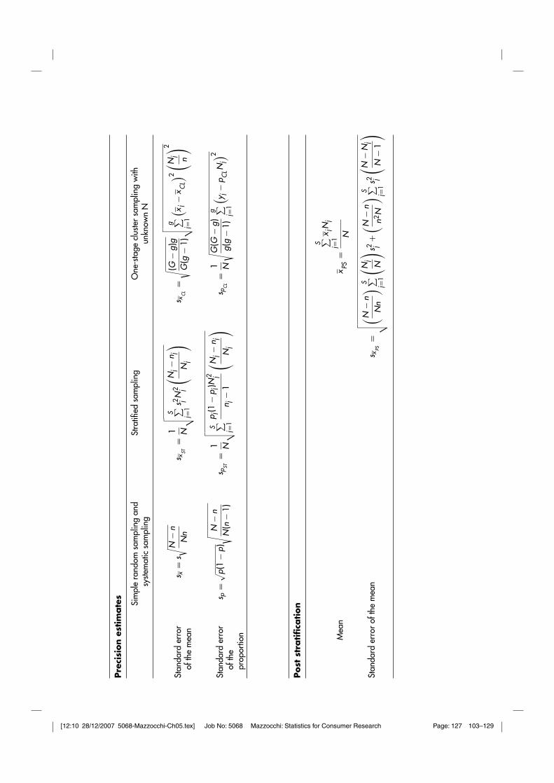
[12:10 28/12/2007 5068-Mazzocchi-Ch05.tex] Job No: 5068 Mazzocchi: Statistics for Consumer Research Page: 127 103–129
Pre
cisi
on
esti
ma
tes
Sim
ple
rand
omsa
mpl
ing
and
syste
mat
icsa
mpl
ing
Stra
tified
sam
plin
gO
ne-s
tage
clus
ter
sam
plin
gw
ithun
know
nN
Stan
dard
erro
rof
the
mea
ns x
=s√ N
−n
Nn
s xST
=1 N
√ √ √ √S ∑ j=1
s2 jN
2 j
( Nj−
n jN
j
)s x
CL
=√ (G
−g)
gG
(g−
1)
√ √ √ √g ∑ j=1
( x j−
x CL) 2(
Nj n
) 2
Stan
dard
erro
rof
the
prop
ortio
n
s p=√ p(
1−
p)
√N
−n
N(n
−1)
s pST
=1 N
√ √ √ √S ∑ j=1
p j(1
−p j
)N2 j
n j−
1
( Nj−
n jN
j
)s p
CL
=1 N
√ G(G
−g)
g(g
−1)
g ∑ j=1
( y j−
p CLN
j) 2
Po
stst
rati
fica
tio
n
Mea
nx PS
=
S ∑ j=1
x jN
j
N
Stan
dard
erro
rof
the
mea
ns x
PS=√ √ √ √( N
−n
Nn
) S ∑ j=1
( Nj
N
) s2 j+( N
−n
n2N
) S ∑ j=1
s2 j
( N−
Nj
N−
1
)
[12:10 28/12/2007 5068-Mazzocchi-Ch05.tex] Job No: 5068 Mazzocchi: Statistics for Consumer Research Page: 128 103–129
128 STATISTICS FOR MARKETING AND CONSUMER RESEARCH
EXERCISES
1) Open the EFS data-set in SPSSa. Compute the mean of the variable cc3111 (clocks, watches and jewellery) on
the whole data-setb. Now, extract a sample of 60 units and compute the sample means using:
i. Simple random samplingii. Stratified sampling (using INCRANGES - income quartiles as stratifica-
tion variable)iii. Systematic sampling
c. What is the sampling error? Which one is the most accurate method? Andthe most precise?
d. Sort the sample by INCANON and perform systematic sampling again –how do results change? Why?
2) Open the Trust data-set in SPSSa. Compute the descriptive statistics of the variable q4kilos on the whole
sample (N = 500)b. Suppose you need to extract a simple random sample of 50 elements, what
is the estimated relative accuracy at a 95% confidence level? (HINT: tα/2 =t0.025 = 1.68)
c. If the target accuracy is ±15%, what is the sample size?3) Open the EFS data-set in SPSS
a. Compute the mean of the variable p609 (recreation expenditure)b. If the distribution of age in the population is the following:
i. Less than 30 = 20%ii. 30–55 = 40%iii. More than 55 = 40%
Post-stratify (using the AGEBIN variable and the proportion above) and compute themean again. Does it differ? Why?
Further readings and web-links
❖ Is random sampling necessary – This chapter has explained the advantagesof random sampling, however scientists are still debating on the extent ofadvantages from sampling. A good discussion is provided in Johnstone(1989).
❖ Good quota sampling – Many studies have looked into the problemsof quota sampling compared to random sampling (see e.g. Moser andStuart, 1953). King (1985) looks at the combination of quota sampling withprobabilistic sampling, with a varying weight of the two methods dependingon the budget constraints. See also the review by Marsh and Scarbrough(1990).
❖ Area sampling – When a sampling frame of the population is not available,a good way to ensure probabilistic extraction is the application of areasampling. See Hansen and Hauser (1945) and Baker (1991).
❖ Failure of non-probability sampling and the effect of non-response –There is an infamous case of survey failure, the prediction of the 1936
[12:10 28/12/2007 5068-Mazzocchi-Ch05.tex] Job No: 5068 Mazzocchi: Statistics for Consumer Research Page: 129 103–129
SAMPLING 129
US elections (Landon vs. Roosevelt). To know more about this story, seethe original results article on the ‘History Matters’ web-site (historymat-ters.gmu.edu/d/5168/) or the actual results from the elections (search onwikipedia.org for ‘United States presidential election, 1936’) and read thepaper by Squire (1988).
Hints for more advanced studies
☞ If you are not convinced about the desirability of probabilistic samplingmethods, how can one test the potential biases of non-probability sampling?Try and build your population data, extract several non-random and randomsamples and compare the performances.
☞ What are the sampling algorithms available in the most popular software forCATI interviews?
☞ This chapter discussed inference on means and variability. However, mostof the times one may want to infer complex relationships from the sampleby using multivariate techniques like regression analysis, cluster analysis,etc… What are the implications for sampling?
Notes
1. See the ‘Further Readings’ section at the end of this chapter for a more advanceddiscussion of the topic of random sampling vs.non-probability sampling.
2. For a review of the essential univariate statistics see the appendix.3. The expected value of an estimator is the average across all possible values of the statistic
and may be interpreted as the average value of the estimator across the sampling space(again, see the appendix for an interpretation of ‘expected values’).
4. A more thorough discussion of the concepts of confidence and significance can be foundin chapter 6.