Sampling in image representation and compression

Dedicated to Paul L. Butzer on the occasion of his 85th birthday

John J. Benedetto and Alfredo Nava-Tudela

November 25, 2013

1 Introduction

1.1 Background

In recent years, interest has grown in the study of sparse solutions of underdetermined systemsof linear equations because of their many and potential applications [11]. In particular, these typesof solutions can be used to describe images in a compact form, provided one is willing to accept animperfect representation.

We shall develop this approach in the context of sampling theory and for problems in imagecompression. These problems arise for a host of reasons including the ever-increasing volume ofimages used in multimedia that, for example, is pervasive in Internet traffic.

The basic idea is the following. Suppose that we have a full-rank matrix A ∈ Rn×m, wheren < m, and that we want to find solutions to the equation,

Ax = b, (1)

where b is a given “signal.” Since the matrix A is full-rank and there are more unknowns thanequations, there are an infinite number of solutions to Equation (1). What if from all possiblesolutions we could find x0, the “sparsest” one, in the sense of having the least number of nonzeroentries? Then, if the number of nonzero entries in x0 happens to be less than the number of nonzeroentries in b, we could store x0 instead of b, achieving a representation x0 of the original signalb in a compressed way. This notion of compression is our point of view, and our presentation isphenomenological and computational, as opposed to theoretical. Our goal is to set the stage foraddressing rigorously the natural questions that arise given this approach.

For example, is there a unique “sparsest” solution to Equation (1)? How does one find such asolution? What are the practical implications of this approach to image compression? How doesresolution of a sparsity problem fit into the context of signal transform compression techniques?For perspective, the JPEG and JPEG 2000 standards have at their core transformations that resultin different representations of the original image which can be truncated to achieve compression atthe expense of some acceptable error [41, 2, 38, 15].

1.2 Finding sparse solutions

The orthogonal matching pursuit (OMP) algorithm is one of the techniques used to find sparsesolutions to systems of linear equations such as Equation (1) [29]. It is one of the greedy algorithmsthat attempts to solve the general problem,

(P ε0) : minx‖x‖0 subject to ‖Ax− b‖2 < ε. (2)

1

Here, ‖x‖0 = #j : |xj | > 0 is the “zero-norm” of vector x, that counts the number of nonzeroentries in x. A greedy algorithm approach is necessary for the solution of the optimization prob-lem defined by (2), since (P ε0) is an NP-complete problem [28]. Moreover, it can be proven thatunder certain circumstances there is a unique sparsest solution to (P ε0); and, under those samecircumstances, OMP is then guaranteed to find it [11]. Generally, OMP will converge to a solutionof Equation (1); but our interest, and the relevance of sampling theory, is contingent on sparsityresults.

1.3 Image representation

To make a practical implementation of the compression idea described in Section 1.1, we followthe approach used in the JPEG and JPEG 2000 standards [41, 2, 38]. Also, in order to test ourimage representation and compression technique, we select a set of four commonly used test images,and review standard image representation concepts.

All images in our database are 512 × 512, 8-bit depth, grayscale images. We proceed to partitioneach image into 64 · 64 = 4096 subsets of 8 × 8 non-overlapping sub-images, and to process eachof these individually. Partitioning a signal to work with more manageable pieces is a commontechnique [44]. Then, we vectorize each 8 × 8 sub-image into a vector b ∈ R64 to be used as a righthand side in Equation (1). There are many ways to do this vectorization and we investigate threeof them.

To complete the setup, we need to choose a matrix A. We begin with A = [DCT1 Haar1] ∈R64×128, where DCT1 is a basis of one-dimensional discrete cosine transform waveforms and Haar1 isa basis of Haar wavelets, respectively. That is, we concatenate two bases of R64, since b ∈ R64. Wealso consider bases for R64 built from tensor products of the one-dimensional waveforms constructedanalogously to the columns of DCT1 and Haar1. This allows us to capture the two-dimensionalnature of an image.

1.4 Outline

In Section 2 we relate our approach to analyze Equation (1) with classical sampling theory.Then, in Section 3 we give the necessary background on OMP for our use in image compression.

In Section 4 we begin by defining the image database, see Section 4.1, and review elementaryimage representation concepts, see Section 4.2. Then, in Section 4.3, we give an overview of imagecompression by sparsity and define the various vectorizations that we use. Finally, in Section 4.4,we provide the details for the various matrices A that we implement.

We shall measure the quality of the reconstruction from compressed representations with thepeak signal-to-noise ratio (PSNR) [38], the structural similarity index (SSIM), and the mean struc-tural similarity index (MSSIM) [42], all as functions of the tolerance ε chosen when solving (P ε0).These concepts are defined in Section 5.

Sections 6, 7, and 8 contain our results in terms of the phenomenological and computationaltheme mentioned in Section 1.1. Section 8 is a recapitulation of all our techniques and goes backto our sampling point of view in Section 2. In particular, we frame compressed sensing withsampling, and introduce deterministic sampling masks, see Section 8.2. We then perform imagereconstruction with them, and do error analysis on the results, see Section 8.3. It remains tointerleaved our results into the structure of general transmission/storage systems in the context ofthe information-theoretical paradigms formulated by Shannon [36].

Section 9 deals with the aforementioned transmission/storage process in terms of quantization,rate, and distortion. We frame our approach to image compression and representation in the setting

2

of transform encoding, and obtain upper bounds on distortion.

2 Sampling theory and Ax = b

The Classical Sampling Formula,

f(t) =∑j

Tf(jT ) s(t− jT ), (3)

was essentially formulated by Cauchy in the 1840s, and, even earlier, Lagrange had formulatedsimilar ideas. The hypotheses of Equation (3) are the following: f ∈ L2(R), the support of itsFourier transform, f , is contained in [−Ω,Ω], where 0 < 2TΩ ≤ 1, and the sampling function s hasthe properties that s ∈ L2(R) ∩ L∞(R) and s = 1 on [−Ω,Ω]. Here, R = R is considered as thedomain of the Fourier transform. One can then prove that Equation (3) is valid in L2−norm anduniformly on R, see [3], Section 3.10. Cauchy’s statement was not quite as general, but the idea ofperiodization which underlies the success of uniform sampling through the years was the same.

Important generalizations, modifications, refinements, and applications of Equation (3) abound.We shall describe how the equation, Ax = b, fits into this context.

A major extension of Equation (3) is to the case,

f(t) =∑j

f(tj) sj(t), (4)

where tj is a non-uniformly spaced sequence of sampled values of f. Because of the non-uniformspacing, the proofs of such formulas can not use periodization methods. In fact, the theory sur-rounding Equation (4) uses deep ideas such as balayage, sophisticated density criteria, and thetheory of frames, see, e.g., the work of Duffin and Schaefer [17], Beurling [7], Beurling and Malli-avin [8, 9], H. J. Landau [25], Jaffard [24] and Seip [35]. A natural extension of the non-uniformsampling Equation (4) is to the case of Gabor expansions,

f(t) =∑j

〈f, τtjeσjg〉 S−1(τtjeσjg), (5)

that are a staple in modern time-frequency analysis, see, e.g., the authoritative [20] and the newbalayage dependent result, [1]. In Equation (5), g is a window function used in the definition ofthe Short Time Fourier Transform, τt denotes translation by t, eσ is modulation by σ, and S−1 isan appropriate inverse frame operator.

It turns out there is a useful Gabor matrix formulation of Equation (5) in the context of Ax = b,see [21, 30].

A discretization of Equation (3), for functions f : Z→ C, could take the form,

f(k) =∑j∈J⊆Z

f(j)aj(k), (6)

for all k ∈ Z, and a given sequence aj of sampling functions aj corresponding to the samplingfunctions aj = τjT s of Equation (3). A similar discretization can be formulated for Equation (4).In both cases, the set J is the domain of sampled values of f from which f is to be characterizedas in Equation (6).

3

Equation (6) can be generalized for a given sequence of sampling functions aj to have the form,

f(k) =∑j∈J⊆Z

x(j)aj(k), (7)

where x(j) = Kf(j) for some operator K : L(Z) → L(Z), e.g., an averaging operator (L(Z)designates a space of functions defined on Z).

To make the tie-in with Equation (1), we write b = f and consider Z/nZ instead of Z; inparticular, we are given b = (b(0), . . . , b(n− 1))T ∈ L(Z/nZ), the space of all functions defined onZ/nZ, and K : L(Z/nz) → L(Z/mZ). Consequently, for #(J) ≤ m, we can define the samplingformula,

∀k ∈ Z/nZ, b(k) =∑

j∈J⊆Z/mZ

x(j)aj(k), (8)

where, x = (x(0), . . . , x(m − 1))T ∈ L(Z/mZ), and where we would like ‖x‖0 < n ≤ m. In thisformat, the sampling formula Equation (8), is precisely of the form Ax = b, and the condition‖x‖0 < n is a desired sparsity constraint. In fact, A = (a0| . . . |am−1), where each column vectoraj = (aj(0), . . . , aj(n− 1))T ∈ Cn = L(Z/nZ).

3 Finding sparse solutions with orthogonal matching pursuit

We give a brief description of the orthogonal matching pursuit (OMP) algorithm in the setting ofsolving (P ε0). Starting from x0 = 0, a greedy strategy iteratively constructs a k-term approximationxk by maintaining a set of active columns—initially empty—and, at each stage, expanding that setby one additional column. The column chosen at each stage maximally reduces the residual `2 errorin approximating b from the current set of active columns. After constructing an approximationincluding the new column, the residual error `2 is evaluated. When it falls below a specifiedthreshold ε > 0, the algorithm terminates. Technically, we proceed as follows.

Task: Find the solution to (P ε0) : minx ‖x‖0 subject to ‖Ax− b‖2 < ε.

Parameters: Given A, b, and ε.

Initialization: Initialize k = 0, and set the following:

• The initial solution x0 = 0;

• The initial residual r0 = b−Ax0 = b;

• The initial solution support S0 = Supportx0 = ∅.Main Iteration: Increment k by 1 and perform the following steps:

• Sweep – Compute the errors ε(j) = minzj ‖zjaj − rk−1‖22 for all j using the optimalchoice z∗j = aTj rk−1/‖aj‖22;

• Update Support – Find a minimizer j0 of ε(j), i.e., for all j /∈ Sk−1, ε(j0) ≤ ε(j),and then update, i.e., set Sk = Sk−1 ∪ j0;• Update Provisional Solution – Compute xk, the minimizer of ‖Ax− b‖22, subject

to Supportx = Sk;• Update Residual – Compute rk = b−Axk;

• Stopping Rule – If ‖rk‖2 < ε, stop; otherwise, apply another iteration.

Output: The proposed solution is xk obtained after k iterations.

4

This algorithm is known in the signal processing literature as orthogonal matching pursuit(OMP) [22, 16, 29, 27, 11], and it is the algorithm we have implemented, validated, and usedthroughout to find sparse solutions of (P ε0).

The notion of mutual coherence gives us a simple criterion by which we can test when a solutionof Equation (1) is the unique sparsest solution. In what follows, we assume that A ∈ Rn×m, n < m,and rank(A) = n.

Definition 1. The mutual coherence of a given matrix A is the largest absolute normalized innerproduct between different columns from A. Thus, denoting the k-th column in A by ak, the mutualcoherence of A is given by

µ(A) = max1≤j,k≤m, j 6=k

|aTj ak|‖aj‖2 · ‖ak‖2

. (9)

Theorem 1. If x solves the system of linear equations Ax = b and ‖x‖0 < 12

(1 + 1/µ(A)

), then

x is the sparsest solution. Hence, if y 6= x also solves the system, then ‖x‖0 < ‖y‖0.

This same criterion can be used to test when OMP will find the sparsest solution.

Theorem 2. For a system of linear equations Ax = b, if a solution x exists obeying ‖x‖0 <12

(1 + 1/µ(A)

), then an OMP run with threshold parameter ε = 0 is guaranteed to find x exactly.

The proofs of these theorems can be found in [11].

4 Image representation and compression

4.1 Image database

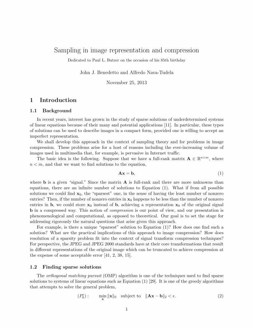
To carry out our experiments and test image compression via sparsity, as well as the propertiesof the matrices described in Section 4.4 for that purpose, we selected 4 natural images, 3 of themfrom the University of Southern California’s Signal & Image Processing Institute (USC-SIPI) imagedatabase [40]. This database has been widely used for image processing benchmarking. The imagesare shown in Figure 1. All images are 512 × 512, 8-bit grayscale images, which means they arecomposed of 5122 = 262,144 pixels that can take integer values from 0 (black) to 255 (white).

4.2 Image representation concepts

For our purposes an image is a two dimensional sequence of sample values,

I[n1, n2], 0 ≤ n1 < N1, 0 ≤ n2 < N2,

having finite extents, N1 and N2, in the vertical and horizontal directions, respectively. The termpixel is synonymous with an image sample value. The first coordinate, n1, is the row index andthe second coordinate, n2, is the column index of the pixel. The ordering of the pixels follows thecanonical ordering of a matrix’s rows and columns, e.g., [38].

The sample value, I[n1, n2], represents the intensity (brightness) of the image at location [n1, n2].The sample values will be B-bit signed or unsigned integers. Thus, we have

I[n1, n2] ∈ 0, 1, . . . , 2B − 1 for unsigned imagery,

I[n1, n2] ∈ −2B−1,−2B−1 + 1, . . . , 2B−1 − 1 for signed imagery.

5

(a) Barbara (b) Boat

(c) Elaine (d) Stream

Figure 1: Images used to test our compression algorithms based on sparse image representation.

6

In many cases, the B-bit sample values are interpreted as uniformly quantized representations ofreal-valued quantities, I ′[n1, n2], in the range 0 to 1 (unsigned) or−1

2 to 12 (signed). Letting round(·)

denote rounding to the nearest integer, the relationship between the real-valued and integer samplevalues may be written as

I[n1, n2] = round(2BI ′[n1, n2]). (10)

This accounts for the sampling quantization error which is introduced by rounding the physicallymeasured brightness at location [n1, n2] on a light sensor to one of the allowed pixel values, e.g.,[38, 44].

We shall use this framework to represent grayscale images, where a pixel value of 0 will represent“black” and a value of 2B − 1 will represent “white”. The value of B is called the depth of theimage, and typical values for B are 8, 10, 12, and 16. Color images are represented by eitherthree values per sample, IR[n1, n2], IG[n1, n2], and IB[n1, n2] each for the red, green, and bluechannels, respectively; other times by luminance IY [n1, n2], blue ICb

[n1, n2], and red ICr [n1, n2]chrominance; or by four values per pixel, IC [n1, n2], IM [n1, n2], IY [n1, n2], and IK [n1, n2], each forthe cyan, magenta, yellow, and black channels commonly used in applications for color printing,respectively. We shall restrict ourselves to grayscale images given that it is always possible to applya compression system separately to each component in turn, e.g., [2, 38].

4.3 Image compression via sparsity

4.3.1 Setup

In this section, we give an overview of image compression via sparsity. The basic idea is that ifAx = b, b is dense—that is, it has mostly nonzero entries—and x is sparse, then we can achievecompression by storing wisely x instead of b.

Specifically, suppose we have a signal b ∈ Rn that requires n numbers for its description.However, if we can solve problem (P ε0), whose solution xε0 has k nonzero entries, with k n, thenwe shall have obtained an approximation b = Axε0 to b using k scalars, with an approximationerror of at most ε. Thus, by increasing ε we can obtain better compression at the expense of alarger approximation error. We shall characterize this relationship between error and compression,or equivalently, error and bits per sample, in Section 7.1.

4.3.2 From an image to a vector to an image

Following the approach to image processing at the core of the JPEG image compression standard[41, 2], we subdivide each image in our database into 8 × 8 non-overlapping squares that will betreated individually. Since we need to generate a right hand side vector b to implement ourcompression scheme via sparsity, cf. Section 4.3.1, a sub-image Y ∈ R8×8 of size 8 × 8 pixels needsto be vectorized into a vector y ∈ R64 to play the role of b. There are many ways to do this, andwe tested three possible approaches.

The first consists of concatenating one after the other the columns of Y to form y, and we shallcall this method c1. It can be thought of as a bijection c1 : R8×8 → R64 that maps Y 7→ y, seeFigure 2(a).

The second approach is to reverse the ordering of the entries of every even column of Y andthen concatenate the columns of the resulting matrix. We shall call this method c2. It is also abijection c2 : R8×8 → R64, see Figure 2(b).

Finally, a third method, c3 : R8×8 → R64, traverses an 8 × 8 sub-image Y in a zigzag patternfrom left to right, see Figure 2(c). It too is a bijection.

7

C1

1 2 3 4

1

2

3

4

(a)

C2

1 2 3 4

1

2

3

4

(b)

C3

1 2 3 4

5 6 7 8

9 10 11 12

13 14 15 16

1259...121516

(c)

Figure 2: Three ways to vectorize a 4× 4 matrix. (a) Concatenate the columns of the matrix fromtop to bottom one after the other, from left to right; or (b) first flip every other column, and thenconcatenate the columns as before; or (c) traverse the elements of the matrix in a Cantor-Peanozigzag fashion. We have shown 4× 4 instead of 8× 8 for ease of illustration.

We must still designate a matrix A ∈ R64×128 to complete the setup. We shall address thisissue in Section 4.4. For now, assume A is given.

Once we have chosen ci and A, we proceed in the following way. Given a tolerance ε > 0, and animage I that has been partitioned into 8 × 8 non-overlapping sub-images Yl, where l = 1, . . . ,Mand M is the number of sub-images partitioning I, we obtain the approximation to yl = ci(Yl)derived from the OMP algorithm, i.e., from the sparse vector xl = OMP(A,yl, ε), we computeyl = Axl. Using yl we can reconstruct a sub-image by setting Yl = c−1i (yl).

Finally, we rebuild and approximate the original image I by pasting together, in the right orderand position, the set Yl of sub-images and form the approximate image reconstruction I of I.This new image I is an approximation, and not necessarily the original image I, because in theprocess we have introduced an error by setting the tolerance ε > 0, and not ε = 0. On the otherhand, we do have ‖y − y‖2 < ε. Since ‖xl‖0 ≤ ‖yl‖0, and more likely ‖xl‖0 ‖yl‖0, storing theset xlMl=1 wisely will provide a compressed representation of the image I.

The means to create efficiently a compressed representation of the image I by using xlMl=1,the map ci : R8×8 → R64, and the matrix A, and analyzing the effects of the choice of the toleranceε on such a representation will be addressed in subsequent sections.

4.4 Choosing a matrix A

4.4.1 Setup

The choice of matrix A is clearly central to our approach to compression. Because of the JPEGand JPEG 2000 standards that use at their core the discrete cosine transform (DCT) and a wavelettransform [41, 2, 38], respectively, we shall incorporate both transforms in our choices of A.

4.4.2 One-dimensional basis elements

Given that the signal that we are going to process comes in the form of a vector b, an inherentlyone-dimensional object, a first approach is to consider the one-dimensional DCT waveforms, andany one-dimensional wavelet basis for L2[0, 1]. For the choice of the wavelet basis we opt for the

8

Haar wavelet and its scaling function, see Equations (12) and (13).More specifically, we know that the one-dimensional DCT-II transform [10, 32],

Xk =N−1∑n=0

xn cos

[π

N

(n+

1

2

)k

], k = 0, . . . , N − 1, (11)

has at its core a sampling of the function fk,N (x) = cos(π(x+ 1

2N

)k)

on the regularly spaced set

S(N) =si ∈ [0 1) : si = i

N , i = 0, . . . , N − 1

of points. We define the vector wk,N =√

2sgn(k) ·

(fk,N (s0), . . . , fk,N (sN−1))T ∈ RN , which we generically call a DCT waveform of wave number k

and length N . We shall use DCT waveforms with N = 64 for the one-dimensional compressionapproach. This is because we subdivide each image in our database into collections of 8 × 8non-overlapping sub-images, which are then transformed into vectors b ∈ R64, and subsequentlycompressed, as described in Section 4.3.2. This collection of DCT waveforms is a basis for R64, andwe arrange its elements column-wise in matrix form as DCT1 = (w0,64 . . .w63,64) ∈ R64×64. Notethat all column vectors of DCT1 have the same `2 norm.

The corresponding basis for R64 based on the Haar wavelet is built in the following way. Considerthe Haar wavelet [26, 33],

ψ(x) =

1 if 0 ≤ x < 1/2,

−1 if 1/2 ≤ x < 1,

0 otherwise,

(12)

and its scaling function,

φ(x) =

1 if 0 ≤ x < 1,

0 otherwise.(13)

For each n ≥ 0, define the set Hn of functions ψn,k(x) = 2n/2ψ(2nx − k), 0 ≤ k < 2n, anddefine H−1 = φ. Note that #Hn = 2n for n ≥ 0 and #H−1 = 1; and therefore #

⋃nj=−1Hj =

1 +∑n

j=0 2j = 2n+1. Since 64 = 26, a value of n = 5 will produce 64 functions to choose from in

H(n) =⋃nj=−1Hj . For each function h ∈ H(5), define the vector vh,64 ∈ R64 by sampling h on the

set S(64), i.e., vh,64 = (h(s0), . . . , h(s63))T. Observe that ‖vh,64‖2 = ‖w0,64‖2 for all h ∈ H(5).

We can order the elements ofH(5) in a natural way, viz., h0 = φ, h1 = ψ0,0, h2 = ψ1,0, h3 = ψ1,1,etc. It is easy to see that the set vhj ,6463j=0 of vectors is a basis for R64. As with the DCTwaveforms, we arrange these vectors column-wise in matrix form as Haar1 = (vh0,64 . . .vh63,64) ∈R64×64.

Then, for the one-dimensional approach, we define A = [DCT1 Haar1] ∈ R64×128, the concate-nation of both bases.

4.4.3 Two-dimensional basis elements

Another way to choose a basis for R64 results from taking into account the intrinsic two-dimensional nature of an image and to define basis elements that reflect this fact. Specifically,consider the two-dimesional DCT-II,

Xk1,k2 =

N1−1∑n1=0

N2−1∑n2=0

xn1,n2 cos

[π

N1

(n1 +

1

2

)k1

]cos

[π

N2

(n1 +

1

2

)k2

], (14)

9

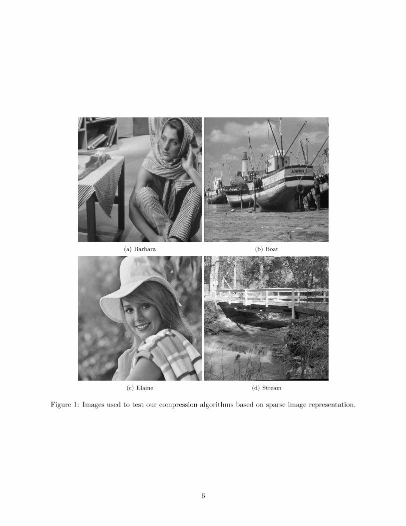
used in the JPEG standard [41, 2]. Consider the family of functions gk1,k2,N1,N2 indexed by k1 andk2, and defined as

gk1,k2,N1,N2(x, y) = cos

[π

(x+

1

2N1

)k1

]cos

[π

(y +

1

2N2

)k2

],

sampled on all points (x, y) ∈ S(N1) × S(N2). In our computations, we take N1 = N2 = 8 andk1, k2 ∈ 0, . . . , 7.

(a) (b)

Figure 3: Natural representation for the 2-dimensional DCT (a) and Haar (b) bases for R64. Whitecorresponds to the maximum value achieved by the basis element, black to the minimum. Theintermediate shade of gray corresponds to 0.

Since gk1,k2,N1,N2(x, y) = fk1,N1(x)fk2,N2(y), the image of S(8) × S(8) under gk1,k2,8,8 can benaturally identified with the tensor product,

wk1,8 ⊗wk2,8, k1, k2 = 0, . . . , 7, (15)

modulo the constants√

2sgn(k1)

and√

2sgn(k2)

, that make ‖wk1,8‖2 = ‖wk2,8‖2, respectively. SeeFigure 3(a) for a graphical representation of all of these tensor products.

There is a total of 64 such tensor products, and for each of them we can obtain a vectorwk1,k2,j = c−1j (wk1,8 ⊗ wk2,8); see Section 4.3.2. It is easy to see that the vector columns of thematrix,

DCT2,j = (wk1,k2,j) ∈ R64×64, k1, k2 = 0, . . . , 7, (16)

form a basis for R64. The ordering of the column vectors of DCT2,j follows the lexicographicalorder of the sequence of ordered pairs (k1, k2) for k1, k2 = 0, . . . , 7 when k2 moves faster than k1,i.e., the ordering is (0,0), (0,1), . . . , (0,7), (1, 0), . . ., (7,7).

In a similar fashion, we can build Haar2,j . Specifically, first consider the setH(2), which contains8 functions. Sampling hk ∈ H(2) on S(8), we obtain the vector vhk,8 ∈ R8. Given k1, k2 ∈ 0, . . . , 7we then compute the vector,

vk1,k2,j = c−1j

(vhk1 ,8 ⊗ vhk2 ,8

)∈ R64,

with which, for all k1, k2 ∈ 0, . . . , 7 and following the same order for the ordered pairs (k1, k2)mentioned above, we can construct

Haar2,j = (vk1,k2,j) ∈ R64×64, k1, k2 = 0, . . . , 7. (17)

10

For a visual representation of the tensor products vhk1 ,8 ⊗ vhk2 ,8, see Figure 3(b).

Finally, we define A = Aj = [DCT2,j Haar2,j ] ∈ R64×128, the concatenation of both bases.

5 Imagery metrics

5.1 Compression and bit-rate

Following the methodology described in Section 4.3.2, suppose that we have an image I of sizeN1 × N2 pixels (N1 = N2 = 512 in our case), and let Yll∈L be a partition of I into #L 8 × 8sub-images. Let yl = ci(Yl) for some i = 1, 2, or 3, where ci : R8×8 → R64, see Figure 2. UsingOMP, with a full-rank matrix A ∈ R64×128 and a tolerance ε > 0, obtain xl = OMP(A,yl, ε), andcompute the approximation to yl given by yl = Axl.

We know that ‖yl − yl‖2 < ε, and we can count how many nonzero entries there are in xl, viz.,‖xl‖0. With this, we can define the normalized sparse bit-rate.

Definition 2 (Normalized Sparse Bit-Rate). Given a matrix A and tolerance ε, the normalizedsparse bit-rate, measured in bits per pixel (bpp), for the image I is the number,

nsbr(I,A, ε) =

∑l ‖xl‖0N1N2

, (18)

where the image I is of size N1 ×N2 pixels.

To interpret this definition, suppose a binary digit or “bit” represents a nonzero coordinate ofthe vector xl. Then we need at least ‖xl‖0 bits to store or transmit xl; and so the total number ofbits needed to represent image I is at least

∑l ‖xl‖0. Thus, the average number of bits per pixel

(bpp) is obtained by dividing this quantity by N1N2. This is the normalized sparse bit-rate.Suppose I is of depth B, and that I can be represented by a string of bits (bit-stream) c. An

important objective of image compression is to assure that the length of c, written length(c), isas small as possible. In the absence of any compression, we require N1N2B bits to represent theimage sample values, e.g. [38]. Thus, the notion of compression ratio is defined as

cr(I, c) =N1N2B

length(c), (19)

and the compressed bit-rate, expressed in bpp, is defined as

br(I, c) =length(c)

N1N2. (20)

The compression ratio is a dimensionless quantity that tells how many times we have managedto reduce in size the original representation of the image, while the compressed bit-rate has bppunits, and it tells how many bits are used on average per sample by the compressed bit-stream cto represent the original image I.

We note from Equations (18) and (20) that it is likely that nsbr(I,A, ε) ≤ br(I, c) if the bit-stream c is derived from the sparse representation induced by A and ε. The rationale for thisassertion is two-fold. First, it is unlikely that the coordinates in each of the resulting xl vectorswill be realistically represented by only one bit, and, second, because c would somehow have toinclude a coding for the indices l for each xl, necessarily increasing the bit count some more. Theseparticular issues, i.e., the number of bits to represent the entries of vectors xl, and the coding ofthe indices l for each of those vectors into a final compressed bit-stream c, will be addressed inSection 9.

11

5.2 Error estimation criteria

Let A = [DCT1 Haar1] and consider the vectorization function c2.Given a 512 × 512 image I in our database, we can proceed to compress it using the method-

ology described in Section 4.3.2. If I is partitioned into 8× 8 non-overlapping sub-images Yl, l =1, . . . , 4096, we obtain for each of them a corresponding reconstructed sub image Yl = c−12 (yl),

and from those we reconstruct an approximation I to I. Here, yl = Axl, xl = OMP(A,yl, ε), andyl = c2(Yl), as before. The compression would come from storing xl efficiently. We summarizethis procedure with the notation, I = rec(I,A, ε).

In order to assess the quality of I when compared to I, we introduce three error estimators.

Definition 3 (PSNR). The peak signal-to-noise ratio between two images I and I is the quantity,

PSNR(I, I) = 20 log10

maxI√mse(I, I)

,

measured in dB, where maxI is the maximum possible value for any given pixel in I (typically,

maxI = 2B−1) and mse(I, I) = 1N1N2

∑i,j

(I[i, j]−I[i, j]

)2is the mean square error between both

images. Here N1 and N2 represent the dimensions of I, and I[i, j] represents the value of the pixelat coordinates [i, j] in image I—similarly for I[i, j]. In our case N1 = N2 = 512, and maxI = 255.

PSNR [38] has the advantage that it is easy to compute and has widespread use, but it hasbeen criticized for poorly correlating with perceived image quality [42, 43]. In recent years extensivework on other error estimators that take into account the human visual system have arisen. Inparticular, we define the structural similarity and mean structural similarity indices [42].

Definition 4 (SSIM). Let I and I be two images that have been decomposed in L × L non-overlapping sub-images, Yl and Yl, respectively. Then the structural similarity index for twocorresponding sub-image vectorizations, say yl = c2(Yl) and yl = c2(Yl), is defined as follows,

SSIM(yl,yl) =(2µyl

µyl+ C1)(2σylyl

+ C2)

(µ2yl+ µ2yl

+ C1)(σ2yl+ σ2yl

+ C2),

where µyland σyl

represent the mean and standard deviation of yl, respectively, with a similardefinition for yl. The term σylyl

is the correlation between yl and yl. The values C1 and C2 aretwo small constants.

For our purposes, we chose the default values of L = 11, C1 = 0.01, and C2 = 0.03 used in[42] when assessing the SSIM of an image in our database and its reconstruction. We used a valueof L = 4 when we modified OMP to use internally the SSIM as a stopping criteria. More on thislater.

From Definition 4, we can see that the SSIM index is a localized quality measure that can berepresented on a plane that maps its values. It can take values from 0 to 1 and when it takes thevalue of 1 the two images are identical. In practice, we usually require a single overall quality ofmeasure for the entire image. In that case we use the mean structural similarity index to evaluatethe overall image quality, defined next.

Definition 5 (MSSIM). Let I and I be two images, where the former is the approximation andthe later is the original. Then the mean structural similarity index is

MSSIM(I, I) =1

M

M∑l=1

SSIM(yl,yl),

12

where yl and yl are vectorizations of sub-images Yl and Yl, respectively. M is the number ofsub-images.

Finally, we take a look at the relationship between the size of the sub-image and the tolerance,and how this affects the quality of the approximation. We analyze the idealized error distributionin which all pixels of the approximation are c units apart from the original. Consider an L×L subimage that has been linearized to a vector y of length L2. Assume that the OMP approximationwithin ε has distributed the error evenly, that is, if x = OMP(A,y, ε) and y = Ax, then

‖Ax− y‖2 < ε⇔ ‖y − y‖22 < ε2,

⇔L2∑j=1

(y(j)− y(j)

)2< ε2,

⇔ L2c2 < ε2,

⇔ c <ε

L. (21)

That is, if we want to be within c units from each pixel, we have to choose a tolerance ε such thatc = ε/L.

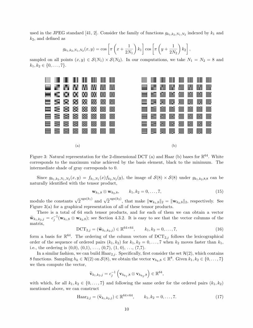
We note that the least-squares approximation at the core of OMP approximates the idealizederror distribution. This can be seen in Figure 4 where the black dashed line represents this idealizederror approximation. For tolerances ε > 40, we see that the PSNR for all images is greater thanthe idealized error distribution. This can be explained by noting that, for example, for ε = 2048,we would have from Equation (21) that c = 2048/8 = 256, but the maximum pixel value isonly 255. Therefore, unless the original image I is just a white patch, the initial value of theOMP approximation being an all black image, there are matching pixels in the original and theapproximation image I = rec(I,A, 2048) that are less than 256 units apart. By Definition 3,this would necessarily imply PSNR(I, I) > 0, a value greater than the value of the PSNR for theidealized error distribution when ε = 2048, which is a small negative value.

On the other hand, for small tolerances, say ε < 3, we observe that the PSNR value for allimages jumps again above the PSNR for the idealized error model. This is a happy case whenroundoff error actually helps. What happens is that for such small tolerances, the roundoff to theclosest integer for all entries in yl = Axl when we form the sub image approximation Yl = c−12 (yl),coincides with the true value of the pixels in the original sub image Yl. Again, by Definition 3,this increases the value of PSNR(I, I) compared to the case where roundoff would not have takenplace.

6 Effects of vectorization on image reconstruction

6.1 Setup

Given an image I in our database, we can follow and apply to it the methodology described inSection 4.3.2, and obtain at the end of this process a reconstructed image I from it. In this sectionwe explore the effects of the choice of map ci : R8×8 → R64 on the characteristics of image I forthe different choices of matrix A that we have selected to study.

6.2 Results for A = [DCT1 Haar1]

We set A = [DCT1 Haar1], and choose a tolerance ε = 32. Then, for each image I in ourdatabase and each index i = 1, 2, 3 we choose the map ci : R8×8 → R64, and follow the methodology

13

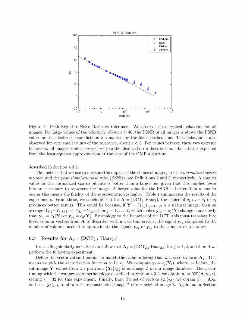
Figure 4: Peak Signal-to-Noise Ratio vs tolerance. We observe three typical behaviors for allimages. For large values of the tolerance, about ε > 40, the PSNR of all images is above the PSNRvalue for the idealized error distribution marked by the black dashed line. This behavior is alsoobserved for very small values of the tolerance, about ε < 3. For values between these two extremebehaviors, all images conform very closely to the idealized error distribution, a fact that is expectedfrom the least-squares approximation at the core of the OMP algorithm.

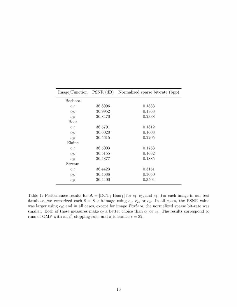
described in Section 4.3.2.The metrics that we use to measure the impact of the choice of map ci are the normalized sparse

bit-rate, and the peak signal-to-noise ratio (PSNR), see Definitions 2 and 3, respectively. A smallervalue for the normalized sparse bit-rate is better than a larger one given that this implies fewerbits are necessary to represent the image. A larger value for the PSNR is better than a smallerone as this means the fidelity of the representation is higher. Table 1 summarizes the results of theexperiments. From these, we conclude that for A = [DCT1 Haar1], the choice of c2 over c1 or c3produces better results. This could be because, if Y = (Yi,j)i,j=1,...,8 is a natural image, then onaverage |Y8,j−Y8,j+1| < |Y8,j−Y1,j+1| for j = 1, . . . , 7, which makes yc2 = c2(Y) change more slowlythan yc1 = c1(Y) or yc3 = c3(Y). By analogy to the behavior of the DFT, this must translate intofewer column vectors from A to describe, within a certain error ε, the signal yc2 compared to thenumber of columns needed to approximate the signals yc1 or yc3 to the same error tolerance.

6.3 Results for Aj = [DCT2,j Haar2,j]

Proceeding similarly as in Section 6.2, we set Aj = [DCT2,j Haar2,j ] for j = 1, 2, and 3, and weperform the following experiment.

Define the vectorization function to match the same ordering that was used to form Aj . Thismeans we pick the vectorization function to be cj . We compute yl = cj(Yl), where, as before, thesub-image Yl comes from the partition Yll∈L of an image I in our image database. Then, con-tinuing with the compression methodology described in Section 4.3.2, we obtain xl = OMP(A,yl, ε),setting ε = 32 for this experiment. Finally, from the set of vectors xll∈L we obtain yl = Axl,and use yll∈L to obtain the reconstructed image I of our original image I. Again, as in Section

14

Image/Function PSNR (dB) Normalized sparse bit-rate (bpp)

Barbarac1: 36.8996 0.1833c2: 36.9952 0.1863c3: 36.8470 0.2338

Boatc1: 36.5791 0.1812c2: 36.6020 0.1608c3: 36.5615 0.2205

Elainec1: 36.5003 0.1763c2: 36.5155 0.1682c3: 36.4877 0.1885

Streamc1: 36.4423 0.3161c2: 36.4686 0.3050c3: 36.4400 0.3504

Table 1: Performance results for A = [DCT1 Haar1] for c1, c2, and c3. For each image in our testdatabase, we vectorized each 8 × 8 sub-image using c1, c2, or c3. In all cases, the PSNR valuewas larger using c2; and in all cases, except for image Barbara, the normalized sparse bit-rate wassmaller. Both of these measures make c2 a better choice than c1 or c3. The results correspond toruns of OMP with an `2 stopping rule, and a tolerance ε = 32.

15

6.2, we assess the effects of the choice of the vectorization function ci by the values of PSNR andnormalized sparse bit-rate resulting from this representation of I by I. We give a summary of theresults of this experiment in Table 2.

We point out that choosing ci, with i 6= j, when Aj = [DCT2,j Haar2,j ], results in worse valuesof both PSNR and normalized sparse bit-rate than when i = j. We record only the results wherei = j.

Moreover, any choice of Aj = [DCT2,j Haar2,j ] with a matching vectorization function cjperforms better than when A = [DCT1 Haar1] for the normalized sparse bit-rate metric, andbetter for the PSNR metric except for the image Stream. Also, on average, the vectorization orderimposed by c3 is slightly better than those by either c1 or c2, although the difference is practicallyimperceptible to the human eye. The normalized sparse bit-rate figures all coincide.

Image/Function PSNR Normalized sparse bit-rate Matrix(dB) (bpp)

Barbarac1 : 37.0442 0.1634 [DCT2,1 Haar2,1]c2 : 37.0443 0.1634 [DCT2,2 Haar2,2]c3 : 37.0443 0.1634 [DCT2,3 Haar2,3]

Boatc1 : 36.6122 0.1541 [DCT2,1 Haar2,1]c2 : 36.6120 0.1541 [DCT2,2 Haar2,2]c3 : 36.6120 0.1541 [DCT2,3 Haar2,3]

Elainec1 : 36.5219 0.1609 [DCT2,1 Haar2,1]c2 : 36.5219 0.1609 [DCT2,2 Haar2,2]c3 : 36.5220 0.1609 [DCT2,3 Haar2,3]

Streamc1 : 36.4678 0.2957 [DCT2,1 Haar2,1]c2 : 36.4676 0.2957 [DCT2,2 Haar2,2]c3 : 36.4677 0.2957 [DCT2,3 Haar2,3]

Table 2: Performance results for Aj = [DCT2,j Haar2,j ], j = 1, 2, 3, with corresponding vectoriza-tion functions c1, c2, and c3. In all cases, the PSNR and normalized sparse bit-rate values werealmost identical. Matrix A3 performs slightly better on average. Mismatching function ci with ma-trix Aj = [DCT2,j Haar2,j ], when i 6= j, results in degraded performance. The values correspondto runs of OMP with an `2 stopping rule, and a tolerance ε = 32.

7 Comparisons between imagery metrics

7.1 Normalized sparse bit-rate vs tolerance

Notwithstanding the remarks in Section 5.1, there is still value in using the normalized bit-stream measure to quantify and plot normalized sparse bit-rate vs tolerance graphs to gauge thecompression properties of various compression matrices.

Given the results in Table 2, we study the compression properties of matrices A = [DCT1 Haar1],

16

(a) Barbara (b) Boat

(c) Elaine (d) Stream

Figure 5: Normalized sparse bit-rate vs tolerance: One-dimensional basis elements. We observethat for all images the best normalized sparse bit-rate for a given tolerance is obtained for matrixA = [DCT1 Haar1] which combines both the DCT1 and Haar1 bases for R64.

17

and A3 = [DCT2,3 Haar2,3]. We compare these properties for both matrices relative to each other,and to the compression properties of B and C, which are formed from the DCT1 or the Haar1 sub-matrices of matrix A, respectively. We plot for all images in our database their respective normal-ized sparse bit-rate vs tolerance graphs. We let ε ∈ T = 2k11k=0∪3, 5, 6, 7, 24, 40, 48, 56, 80, 96, 112and for each image I in our image database we obtained the corresponding normalized sparse bit-rates nsbr(I,A, ε), nsbr(I,B, ε), and nsbr(I,C, ε) to obtain the plots in Figure 5. In Figure 6we compare A = [DCT1 Haar1] with A3 = [DCT2,3 Haar2,3]. We observe that up to a toleranceεI , dependent on image I, A3 performs better for tolerance values ε ≥ εI . That is, the value ofthe normalized sparse bit-rate is smaller when performing compression utilizing A3. For values ofε ≤ εI , compression with A results in better normalized sparse bit-rate values. We shall see inSection 7.2, with the aid of Figure 4, that for values of ε = 32, and smaller, the quality of the imagereconstruction is satisfactory. We note from Figure 6 that, for all images in our database, εI < 32.This means that, for most practical cases, the use of [DCT2,3 Haar2,3] results in slightly smallernormalized sparse bit-rate values than when using [DCT1 Haar1].

(a) Barbara (b) Boat

(c) Elaine (d) Stream

Figure 6: Normalized sparse bit-rate vs tolerance: Comparison between A = [DCT1 Haar1] andA3 = [DCT2,3 Haar2,3].

From the results shown in Figure 5, we can see that the DCT1 basis elements perform better

18

compression for any given tolerance than when using the Haar1 basis elements, except for imageStream. In fact, when the tolerance ε is close to but less than 3, the Haar1 basis elements result ina smaller normalized sparse bit-rate value. Moreover, and more importantly, combining both theDCT1 and Haar1 bases results in better compression than if either basis is used alone. The sameis true for DCT2,3 and Haar2,3.

In this light, there are natural questions dealing with and relating image reconstruction quality,range of effective tolerances, and error estimators.

7.2 PSNR vs MSSIM

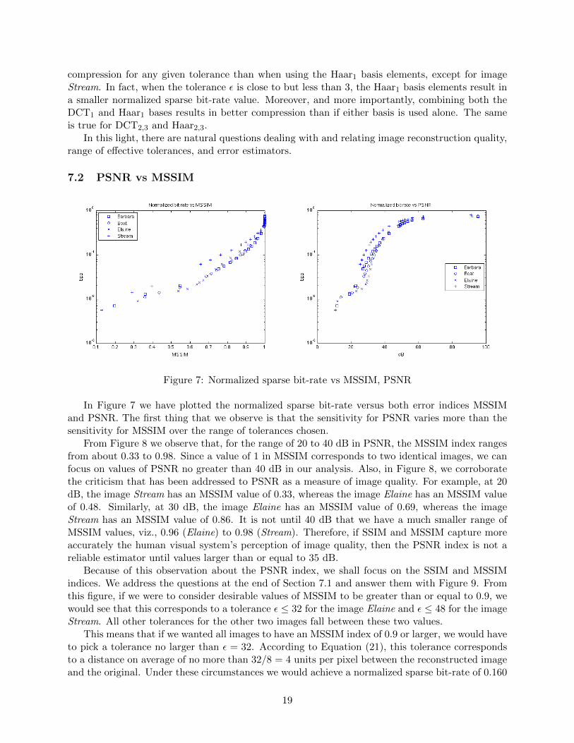
Figure 7: Normalized sparse bit-rate vs MSSIM, PSNR

In Figure 7 we have plotted the normalized sparse bit-rate versus both error indices MSSIMand PSNR. The first thing that we observe is that the sensitivity for PSNR varies more than thesensitivity for MSSIM over the range of tolerances chosen.

From Figure 8 we observe that, for the range of 20 to 40 dB in PSNR, the MSSIM index rangesfrom about 0.33 to 0.98. Since a value of 1 in MSSIM corresponds to two identical images, we canfocus on values of PSNR no greater than 40 dB in our analysis. Also, in Figure 8, we corroboratethe criticism that has been addressed to PSNR as a measure of image quality. For example, at 20dB, the image Stream has an MSSIM value of 0.33, whereas the image Elaine has an MSSIM valueof 0.48. Similarly, at 30 dB, the image Elaine has an MSSIM value of 0.69, whereas the imageStream has an MSSIM value of 0.86. It is not until 40 dB that we have a much smaller range ofMSSIM values, viz., 0.96 (Elaine) to 0.98 (Stream). Therefore, if SSIM and MSSIM capture moreaccurately the human visual system’s perception of image quality, then the PSNR index is not areliable estimator until values larger than or equal to 35 dB.

Because of this observation about the PSNR index, we shall focus on the SSIM and MSSIMindices. We address the questions at the end of Section 7.1 and answer them with Figure 9. Fromthis figure, if we were to consider desirable values of MSSIM to be greater than or equal to 0.9, wewould see that this corresponds to a tolerance ε ≤ 32 for the image Elaine and ε ≤ 48 for the imageStream. All other tolerances for the other two images fall between these two values.

This means that if we wanted all images to have an MSSIM index of 0.9 or larger, we would haveto pick a tolerance no larger than ε = 32. According to Equation (21), this tolerance correspondsto a distance on average of no more than 32/8 = 4 units per pixel between the reconstructed imageand the original. Under these circumstances we would achieve a normalized sparse bit-rate of 0.160

19

Figure 8: Peak Signal-to-Noise Ratio vs Mean Structural Similarity

Figure 9: Normalized sparse bit-rate and corresponding MSSIM vs tolerance. In this graph wehave plotted together the best normalized sparse bit-rate obtained by combining the DCT andHaar bases, and the corresponding value of the MSSIM index for a given tolerance. The normalizedsparse bit-rate graphs are on the bottom left, and the MSSIM index values are above these.

20

to 0.305 bits per pixel. It is natural to ask if there is a modification of OMP which guarantees acertain minimum MSSIM quality level. It turns out that such a modification is possible.

Consider the following change to the stopping rule, ‖Ax− b‖2 < ε, for the OMP algorithm:

‖Ax− b‖MSSIM ≡ MSSIM(c−12 (Ax), c−12 (b)) > δ0,

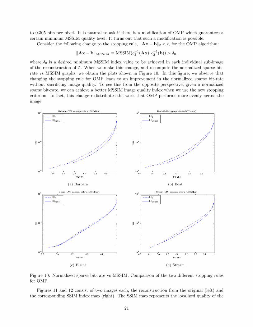
where δ0 is a desired minimum MSSIM index value to be achieved in each individual sub-imageof the reconstruction of I. When we make this change, and recompute the normalized sparse bit-rate vs MSSIM graphs, we obtain the plots shown in Figure 10. In this figure, we observe thatchanging the stopping rule for OMP leads to an improvement in the normalized sparse bit-ratewithout sacrificing image quality. To see this from the opposite perspective, given a normalizedsparse bit-rate, we can achieve a better MSSIM image quality index when we use the new stoppingcriterion. In fact, this change redistributes the work that OMP performs more evenly across theimage.

(a) Barbara (b) Boat

(c) Elaine (d) Stream

Figure 10: Normalized sparse bit-rate vs MSSIM. Comparison of the two different stopping rulesfor OMP.

Figures 11 and 12 consist of two images each, the reconstruction from the original (left) andthe corresponding SSIM index map (right). The SSIM map represents the localized quality of the

21

image reconstruction. Lighter values are values closer to 1 (“white” = 1), whereas darker valuesare values closer to 0 (“black” = 0). Using the image of the Boat as our image I, we obtained areconstruction I1 with ε = 32 for the `2 stopping criterion, and a reconstruction I2 for the MSSIMstopping criterion choosing δ0 < MSSIM(I1, I) in such a way that MSSIM(I2, I) ' MSSIM(I1, I).

(a) Boat (b) SSIM

Figure 11: Boat: ε = 32, PSNR = 36.6020 dB, MSSIM = 0.9210, normalized sparse bit-rate =0.1608 bpp, stopping rule: ‖ · ‖2.

(a) Boat (b) SSIM

Figure 12: Boat: δ0 = 0.92, PSNR = 34.1405 dB, MSSIM = 0.9351, normalized sparse bit-rate =0.1595 bpp, stopping rule: ‖ · ‖MSSIM .

22

8 Sampling in image representation and compression

8.1 Compressed sensing and sampling

Our approach to image representation and our treatment of images for compression lends itselfto experimentation in the area of compressed sensing. With a slight modification of the classicalcompressed sensing technique, we shall show how to construct deterministic sampling masks inorder to sample an original image and recover an approximation having a controllable signal-to-noise ratio. This technique can be interpreted in two ways, either as a classical compressed sensingproblem or as a non-uniform sampling reconstruction problem, see Section 8.3.

For signals that are sparsely generated, the classical compressed sensing paradigm can be sum-marized as follows. Consider a random matrix P ∈ Rk×n with Gaussian i.i.d. entries, and supposethat it is possible to directly measure c = Pb, which has k entries, rather than b, which has n.Then we solve

minx‖x‖0 subject to ‖PAx− c‖2 ≤ ε, (22)

to obtain a sparse representation xε0, and synthesize an approximate reconstruction b ≈ Axε0, wherexε0 is a solution to Problem (22) [11].

We make the following observations about this technique. If one literally generates a randommatrix P ∈ Rk×n, we would expect with probability 1 that PA ∈ Rk×m would be full-rank, giventhat we have assumed all along that A ∈ Rn×m is such, and that ‖xε0‖0 ≤ k ≤ n. A desirable featurefrom this approach would be that if k = n, we should obtain the same representation xε0 as if we hadsolved (P ε0) directly, see Problem (2), with the dictionary set to PA instead of A, and the signalb set to Pb. In this case, if P were an isometry, then ‖Axε0 − b‖2 = ‖PAxε0 − Pb‖2 ≤ ε and wewould have the same signal-to-noise ratio, or equivalently, normalized sparse bit-rate vs tolerance,image reconstruction/representation characteristics as if we had performed a direct measurementof b. But in general, ‖Axε0 − b‖2 6= ‖PAxε0 − Pb‖2. Hence, if we want to have the desirableproperty of recovering the solution to (P ε0) when k = n, then we must pay particular attention tothe construction of P. Moreover, having a particular matrix P does not tell us anything on howto actually sample b, but we assume that somehow, we can obtain the signal c to treat with ouralgorithms.

8.2 Deterministic sampling masks

To overcome the shortcomings inherent to the classical compressed sensing approach mentionedabove, we propose the use of deterministic sampling masks, which we define next.

Consider an 8×8 sub-image Y of an image I, and an 8×8 matrix M whose entries are either 0or 1. We can choose the values of M at random or in a deterministic way. We choose a hybrid, thatis, we preset the number of entries in M that will be zero, but choose their location at random. Inthis case, we shall call M a deterministic sampling mask. Let k be the number of entries in M thatare equal to 1, then the ratio of k to the the total number of entries in M is called the density ofM, k/64 in this case. We denote it by ρ(M). Reciprocally, we say that 64−k

64 is the sparsity of M.Now we choose a vectorization function, say c3, see Section 4.3.2, and apply it both to the

sub-image Y and mask M, and obtain a vector w = (w1, . . . , w64)T ∈ R64 equal to the entry-wise

product c3(Y)⊗ c3(M). Finally, given both w and c3(M), we perform a dimension reduction h onw by collapsing its entries where c3(M) vanishes, obtaining c ∈ Rk. In function form, we have

h : R64 × R64 → Rk

h(w, c3(M)) = (wj1 , . . . , wjk)T, (23)

23

with j1 < · · · < jk and supp(c3(M)) = ji. We call c = h(c3(Y), c3(M)) the masking of Y by M.If b = c3(Y) and c = h(b, c3(M)), we will also say that c is the masking of b by M.

It is easy to see that if the density ρ(M) = 1, then h(b, c3(M)) = b for any b ∈ R64. Thisfact will help us achieve the goal of obtaining identical solutions to Problems (2) and (22) whenρ(M) = 1, overcoming one of the main shortcomings we had mentioned in Section 8.1, as seen inthe next section.

8.3 Image reconstruction from deterministic sampling masks and error analysis

(a) Original (b) Masked original

(c) Reconstruction from (b) (d) SSIM between (a) and (c)

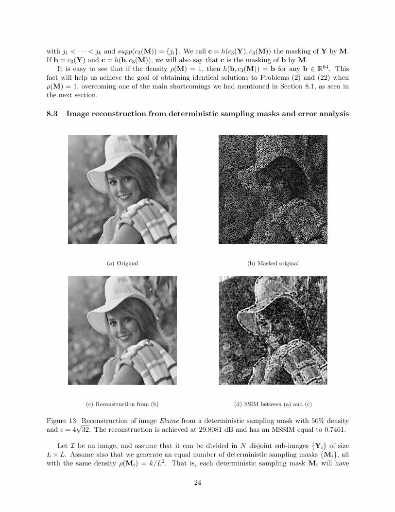
Figure 13: Reconstruction of image Elaine from a deterministic sampling mask with 50% densityand ε = 4

√32. The reconstruction is achieved at 29.8081 dB and has an MSSIM equal to 0.7461.

Let I be an image, and assume that it can be divided in N disjoint sub-images Yi of sizeL× L. Assume also that we generate an equal number of deterministic sampling masks Mi, allwith the same density ρ(Mi) = k/L2. That is, each deterministic sampling mask Mi will have

24

exactly k entries equal to 1. Then choose a vectorization function, say c3, cf. Section 4.3.2, andform the masking ci of bi = c3(Yi) by Mi for all N sub-images with their respective mask.

With this setup, we are ready to propose a way to recover image I from ci. For eachi ∈ 1, . . . , N, let xε0,i be the solution to the problem

minx‖x‖0 subject to ‖h(Ax, c3(Mi))− ci‖2 ≤ ε, (24)

and recover a reconstruction I of I by assembling in correct order the sub-images generated by thesparse representations xε0,i, that is, I is formed by putting together in proper sequence the set of

sub-image reconstructions c−13 (Axε0,i). See Figure 13 for an example of this technique in action.A few observations are in order. First, note that we can identify Problem (22) with Problem

(24), if we identify PAxε0,i ≡ h(Axε0,i, c3(Mi)). This way, if the density ρ(Mi) = 1 for all i, giventhat h(Axε0,i, c3(Mi)) = Axε0,i—from the observation made at the end of the previous section—Problem (24), and therefore Problem (22), would be identical to Problem (2), as desired. Hence,Problem (24) is a generalization of Problem (2).

(a) Total variation (b) Number of iterations

(c) Exonorm (d) Endonorm

Figure 14: Total variation, performance, and error metrics for the reconstruction of Elaine by wayof deterministic sampling masks. Density is set to 50%, ε = 4

√32, and dictionary A = [DCT2,3].

Second, we can say a few words regarding the choice of ε in Problem (24), since this parameter

25

controls the compression and, to a degree, the error characteristics of the reconstruction image I.From the choice of deterministic sampling matrices that we made, the effective dimension of thevectors ci that we are trying to approximate is k, that is, ci ∈ Rk for all i. Bearing in mind thatci can be thought of as the representation of a sub-image of size

√k×√k via a similar vectorization

function in the spirit of, say c3, as was done here, the value of ε determines the error of the resultingapproximation h(Axε0,i, c3(Mi)) to ci constructed here. From the error analysis and interpretationdone for Equation (21), we can then compute the value of ε given a target idealized uniform errordistribution. For example, if we want on average to be at no more than 4 units away from theactual value of each pixel in the image represented by ci, we must choose ε = 4

√k. If, as in our

example in Figure 13, we have partitioned our image in 8× 8 sub-images, and chosen a density of50%, this would give a value of ε = 4

√32. Then, the error between the points in Yi represented by

ci and h(Axε0,i, c3(Mi)) would be on average no more than 4 units per pixels. In fact, the `2 norm

of h(Axε0,i, c3(Mi)) − ci, will be less than or equal to 4√

32. We call this error the endonorm forsub-image Yi.

However, we cannot yet say much about the error outside the pixels not represented by ciin the original sub-image. This error will be given by ‖Axε0,i − bi‖2 − ‖h(Axε0,i, c3(Mi)) − ci‖2,which we call the exonorm for sub-image Yi. It is clear from these definitions that the total error‖Axε0,i−bi‖2 for the approximation of sub-image Yi by c−13 (Axε0,i) is the sum of its endo- and exo-norms. As we established above, we have exact control of the endonorm by the choice of ε, but nonwhatsoever of the exonorm. We speculate that the magnitude of the exonorm of any given sub-image Yi is linked to the choice of dictionary A, and the total variation V (bi)

.=∑n−1

j=1 |bj+1 − bj |,of bi = (b1, . . . , bn)T. In Figure 14 we show four maps, each showing the value of a given metricthat each sub-image that makes up image Elaine has, for each of the four metrics we consider.The metrics are the total variation, the number of iterations that it took OMP to converge to thedesired error tolerance of ε = 4

√32 ≈ 22.63 in Equation (24), the exonorm, and the endonorm.

Note that in Figure 14(d) the endonorm is less than or equal to the desired error tolerance.Observe the correlation that the number of iterations, Figure 14(b), and the exonorm, Figure14(c), seem to have with the total variation, Figure 14(a), of each sub-image. In this case, we setA = [DCT2,3]. When we try A = [DCT2,3 Haar2,3] the results show an increase in the exonorm,which impacts negatively both PSNR and MSSIM error measures, although the normalized sparsebit-rate is slightly smaller, as expected. This confirms that the choice of dictionary A has an impacton the error of the reconstruction from deterministic sampling masks.

Finally, we mention that since all masks have the same density, the overall sampling densityfor the original image is k/L2, which means that a total of kN points are sampled, as opposed toL2N , had we sampled all points in the image to reconstruct it. Moreover, the sampling is doneat random. Hence, what starts as a compressed sensing problem can be seen as a non-uniformsampling reconstruction problem.

9 Quantization

9.1 Background

As a precursor to Shannon, Hartley wrote the following equation to quantify “information” ina discrete setting:

H = n log s,

where H is the amount of information, n is the number of symbols transmitted, and s is the sizeof a given alphabet from which the symbols are drawn [18]. Shannon extended this notion by

26

identifying the amount of information with entropy, see [36]. Specifically, in the case of a discreteinformation source, Shannon represented it as a Markov process, and asked if one could “define aquantity which will measure, in some sense, how much information is ‘produced’ by such a process,or better, at what rate information is produced”. In fact, he defined this quantity H in terms ofentropy as

H = −n∑i=1

pi log2 pi, (25)

where we suppose that we have a set of n possible events whose probabilities of occurrence arep1, p2, . . . , pn.

To interpret Equation (25) we assume that we are given a random variable X on the finite set1, 2, . . . , n with probability distribution p. The elements X(1) = x1, X(2) = x2, . . . , X(n) = xnare distinct and p(x1), p(x2), . . . , p(xn) are nonnegative real numbers with p(x1) + p(x2) + . . . +p(xn) = 1. We write pi = p(xi) as a shorthand for prob(X = xi). The smaller the probability p(xi),the more uncertain we are that an observation of X will result in xi. Thus, we can regard 1/p(xi)as a measure of the uncertainty of xi. The smaller the probability, the larger the uncertainty, see[36, 31, 23]. Shannon thought of uncertainty as information. In fact, if an event has probability 1,there is no information gained in asking the outcome of such an event given that the answer willalways be the same.

Consequently, if we define the uncertainty of xi to be − log2 p(xi), measured in bits, the entropyof the random variable X is defined to be the expected value,

H(X) = −n∑i=1

p(xi) log2 p(xi),

of the uncertainty of X, i.e., the entropy of X will measure the information gained from observingX.

Further, Shannon defined the capacity C of a discrete noiseless channel as

C = limT→∞

logN(T )

T,

where N(T ) is the number of allowed signals of duration T .

Theorem 3 (Shannon, Fundamental Theorem for a Noiseless Channel [36]). Let a source haveentropy H (bits per symbol) and let a channel have a capacity C (bits per second). Then it ispossible to encode the output of the source in such a way as to transmit at the average rate C

H − εsymbols per second over the channel where ε is arbitrarily small. It is not possible to transmit atan average rate greater than C

H .

This existential result has been a driving force for developing constructive quantization andcoding theory through the years, e.g., [19] for an extraordinary engineering perspective and high-lighting the role of redundancy in source signals, cf. the theory of frames [4, Chap. 3 and 7] and[6, 14, 13].

9.2 Quantization (coding), rate, and distortion

A scalar quantizer is a set S of intervals or cells Si ⊂ R, i ∈ I, that forms a partition of the realline, where the index set I is ordinarily a collection of consecutive integers beginning with 0 or 1,

27

together with a set C of reproduction values or levels yi ∈ R, i ∈ I, so that the overall quantizer qis defined by q(x) = yi for x ∈ Si, expressed concisely as

q(x) =∑i∈I

yi1Si(x), (26)

where the indicator function 1S(x) is 1 if x ∈ S and 0 otherwise [19, 12].More generally, a class of memoryless quantizers can be described as follows. A quantizer of

dimension k ∈ N takes as input a vector x = (x1, . . . , xk)T ∈ A ⊆ Rk. Memoryless refers to a

quantizer which operates independently on successive vectors. The set A is called the alphabet orsupport of the source distribution. If k = 1 the quantizer is scalar, and, otherwise, it is vector. Thequantizer then consists of three components: a lossy encoder α : A → I, where the index set I isan arbitrary countable set; a reproduction decoder β : I → A, where A ⊂ Rk is the reproductionalphabet; and a lossless encoder γ : I → J , an invertible mapping (with probability 1) into acollection J of variable-lenght binary vectors that satisfies the prefix condition, that is, no vectorin J can be the prefix of any other vector in the collection [19].

Alternatively, a lossy encoder is specified by a scalar quantizer S = Si ⊂ R : i ∈ I of A; areproduction decoder is specified by a codebook C = β(i) ∈ A : i ∈ I of points, codevectors, orreproduction codewords, also known as the reproduction codebook; and the lossless encoder γ can bedescribed by its binary codebook J = γ(i) : i ∈ I containing binary or channel codewords. Thequantizer rule is the function q(x) = β(α(x)) or, equivalently, q(x) = β(i) whenever x ∈ Si [19].

The instantaneous rate of a quantizer applied to a particular input is the normalized lengthr(x) = 1

k l(γ(α(x))) of the channel codeword, the number of bits per source symbol that must besent to describe the reproduction. If all binary codewords have the same length, it is referred to asa fixed-length or fixed-rate quantizer.

To measure the quality of the reproduction, we assume the existence of a nonnegative distortionmeasure d(x, x) which assigns a distortion or cost to the reproduction of input x by x. Ideally,one would like a distortion measure that is easy to compute, useful in analysis, and perceptuallymeaningful in the sense that small (large) distortion means good (poor) perceived quality. No singledistortion measure accomplishes all three goals [19]. However, d(x, x) = ‖x− x‖22 satisfies the firsttwo.

We also assume that d(x, x) = 0 if and only if x = x. In this light we say that a code is losslessif d(x, β(α(x))) = 0 for all inputs x, and lossy otherwise.

Finally, the overall performance of a quantizer applied to a source is characterized by thenormalized rate,

R(α, γ) = E[r(X)] =1

kE[l(γ(α(X)))]

=1

k

∑i

l(γ(i))

∫Si

f(x) dx, (27)

and the normalized average distortion,

D(α, β) =1

kE[d(X,β(α(X)))]

=1

k

∑i

∫Si

d(x,yi)f(x) dx. (28)

Here, we assume that the quantizer operates on a k-dimensional random vector X = (X1, . . . , Xk)that is described by a probability density function f . Every quantizer (α, γ, β) is thus described by

28

a rate-distortion pair (R(α, γ), D(α, β)). The goal of a compression system design is to optimizethe rate-distortion trade-off [19].

In light of the results by Shannon in Section 9.1, compression system design will also have totake into account the characteristics of the communication channel in managing the rate-distortiontrade-off. Also, from the definitions above, it is clear that knowledge of the probability densityfunction of the source messages is relevant, see Figure 15.

(a) (b)

(c) (d)

(e) (f)

Figure 15: Histograms for images Boat, Elaine and a uniform random input. Figures (a), (c), and(e) are the histograms for the choice of columns of A, labeled from left to right, 1 to 128, andFigures (b), (d), and (f) show the set of coefficient values chosen for each column, labeled in asimilar way. We set the tolerance ε = 32, and used A3 = [DCT2,3 Haar2,3].

29

9.3 Image quantization and encoding

With the perspective from Sections 9.1 and 9.2, we return to the topic of image quantizationand encoding with regard to compression. The image standards, JPEG and JPEG 2000, are framedin the transform coding paradigm, and contain two steps beyond their respective discrete cosinetransform (DCT) and the Cohen-Daubechies-Feauveau 5/3 (lossless) and 9/7 (lossy) biorthogonalwavelet transforms. Both have quantization (α) and encoding (γ) steps, with their respective“inverses”, to complete their definitions [41, 2, 38, 15].

The general schematic for transform coding is described in Figure 16.

T Q E

T' Q' E'

b

b'

Storage/Transmission

Figure 16: Schematic diagram of a general transform coding system.

Example 1. The transform T is meant to exploit the redundancy in the source signal b anddecorrelate it. It has an inverse T−1 or, minimally, a left inverse T ′ such that T ′Tb = b. In ourapproach we have A = T ′, and T is defined via OMP by Tb = OMP(A,b, ε0). Thus, we have‖T ′Tb−b‖2 < ε. Therefore, our compression scheme is lossy. Q is a non-invertible scalar quantizerthat will be applied to the coefficients of the vector Tb, and Q′ is its reproduction function. Finally,we have an invertible lossless encoder E, defined as γ in the previous section, with E′ = E−1. Thecomposition QT is equivalent to the lossy encoder α, and the composition T ′Q′ corresponds to thereproduction decoder β from Section 9.2.

In order to describe the overall performance of our quantizer, (α, γ, β) = (QT,E, T ′Q′), wemust characterize the rate-distortion pair (R(QT,E), D(QT, T ′Q′)).

Proposition 4. Let n < m and let A = (aj) ∈ Rn×m be a full-rank matrix with each ‖aj‖2 = c.Given a > 0 and y ∈ Rn. Suppose that x ∈ Rm has the property that aAx = y and that ε ∈ Rmsatisfies ‖ε‖0 ≤ ‖x‖0. If x = x + ε and y = aAx, then

‖y − y‖2 ≤ ac‖ε‖∞‖x‖0. (29)

Proof. Let ε = (ε1, . . . , εm)T ∈ Rm with ‖ε‖0 ≤ ‖x‖0 and let x = x + ε. Then, we compute

‖y − y‖2 = ‖aAx− aAx‖2 = a‖A(x + ε)−Ax‖2

= a‖Aε‖2 = a∥∥∥ m∑j=1

ajεj

∥∥∥2

= a∥∥∥∑εj 6=0

ajεj

∥∥∥2

≤ a∑εj 6=0

‖ajεj‖2 = a∑εj 6=0

‖aj‖2|εj | = a∑εj 6=0

c|εj |

≤ a∑εj 6=0

c‖ε‖∞ = ac‖ε‖∞‖ε‖0 ≤ ac‖ε‖∞‖x‖0.

30

Remark 1. a. In Proposition 4, the value of ‖ε‖0 is linked to the sparsity of x, because in our casethe error ε comes from scalar quantizing the entries of x. That is, if x = round(x), where x is thevector whose entries are exactly those of x but rounded to the closest integer, then, necessarily,

‖ε‖0 = ‖x− x‖0 ≤ ‖x‖0. (30)

Hence, in the case where a scalar quantization scheme satisfies Inequality (30), Proposition 4 gives

‖y − y‖2 ≤ ac‖ε‖∞‖x‖0, (31)

with A = (aj), y = aAx, y = aAx, and c = ‖aj‖2 for all j. Observe that, in particular, whenx = round(x), we have ‖ε‖∞ = 1/2.

From Inequality (31) we see that the error in the reconstruction due to scalar quantization islinked to the size of c, ‖ε‖∞, and the sparsity of x. We are tempted to make c as small as possible,or modify the quantization scheme to make ‖ε‖∞ smaller to reduce the reconstruction error due toscalar quantization.

b. If x0 is the sparsest vector that solves Ax = y, then a−1x0 is the sparsest vector that solvesaAx = y, and ‖x0‖0 = ‖ax0‖0. We conclude that the norm of a−1x0 has an inversely proportionalrelationship with the size of a. Therefore, if we are to use a finite predetermined number of bits torepresent a−1x0, the solution of aAx = y, we necessarily have a constraint on a.

c. We know that the magnitude of the coordinates of x are bounded by a multiple of ‖y‖2, see[5]. This has an impact on how many bits are needed to represent x. Therefore, when choosing ain Proposition 4 we have to take into consideration the maximum value that the value of ‖y‖2 willimpose on the magnitude of the coordinates of x, see Examples 2 and 3.

Finally, recall that our image compression approach comes from the OMP solution x0 to problem(P ε00 ) for a given matrix A = (aj) whose column vectors satisfy ‖aj‖2 = c, where b is a given vector,and for which ‖Ax0 − b‖2 < ε0 for the given tolerance ε0. Then, choosing a > 0, and followingthe description of T at the beginning of this section, if we set x0 = Tb = OMP(aA,b, ε0) for agiven signal b and a tolerance ε0 > 0, aA = T ′, Q a scalar quantizer that satisfies Inequality‖ε‖0 = ‖Q(x)−x‖0 ≤ ‖x‖0, and Q′ its corresponding reproduction function, the triangle inequalityand Inequality (29) give

d(β(α(b)),b) = ‖T ′Q′QTb− b‖2= ‖T ′Q′QTb− T ′Tb + T ′Tb− b‖2= ‖aAx0 − aAx0 + aAx0 − b‖2≤ ‖aAx0 − aAx0‖2 + ‖aAx0 − b‖2= ac‖δ‖∞‖x0‖0 + ε0,

where δ = x0 − x0. This inequality would give us a footing in the computation of the normalizedaverage distortion D(α, β), see Equation (28).

Example 2. From the definition of D(α, β), it is clear that we need to know something aboutthe probability density function of the input sources, i.e., the statistics of the 8× 8 vectorized sub-images into which each image is partitioned, if we are to compute D. In place of such knowledge,we can observe the distribution of the coefficients for each of the vectors resulting from the analysisof the images in our database and their corresponding histograms. This is what Figure 15 shows.For each such image I, we used the matrix A3 = [DCT2,3 Haar2,3] = (ai) with a tolerance ofε = 32 to compute its statistics. On the x-axis of each subfigure in Figure 15 we have matched

31

column ai at position i to the integer i. Hence, positions 1 to 64 correspond to the DCT waveforms,and positions 65 to 128 to the Haar waveforms. All subfigures on the left are the histograms forthe frequency with which each column vector of A3 is chosen. For example, since there are 4096sub-images of size 8 × 8 in a 512 × 512 image, the column vector a1 will be chosen 4096 timessince it corresponds to the constant vector, which computes the mean or DC component for eachsub-image. All subfigures to the right correspond to partial representations of the distribution ofthe coefficients that multiply each and every column vector whenever such a vector is chosen in therepresentation/approximation of an input b. For example, suppose that column a74 was multipliedby a coefficient a74 = 3.2310 to obtain the representation of some input b = a74a74 + r within atolerance of ε = 32. Then we would have plotted point (74, 3.2310) in its corresponding subfigure tothe right. We have not plotted the coefficients for a1 since they correspond to the DC componentsof the sub-images of I, which vary between 0 and 255. We note that all images in our databasehave a similar structure.

Example 3. For comparison purposes, we obtained the histogram and the distribution of coef-ficients for a randomly generated image with a uniform distribution on [0 255], see Figures 15(e)and 15(f). The first thing we note is that unlike the natural images in our database, all columnvectors, except a1 and a65, which correspond to the constant vectors (one for the DCT and onefor the Haar waveforms), are chosen about the same number of times regardless of their position.Further, the distribution of the values of the coefficients is uniform. It is also clear that, in order tobe reconstructed, this is the image that requires the most nonzero coefficients within the toleranceε = 32. This is consistent with the definition of information by Shannon: the more the uncertaintyin a source, the more information it carries.

(a) (b)

Figure 17: (a) MSSIM vs Normalized sparse bit-rate, (b) PSNR vs Normalized sparse bit-rate.

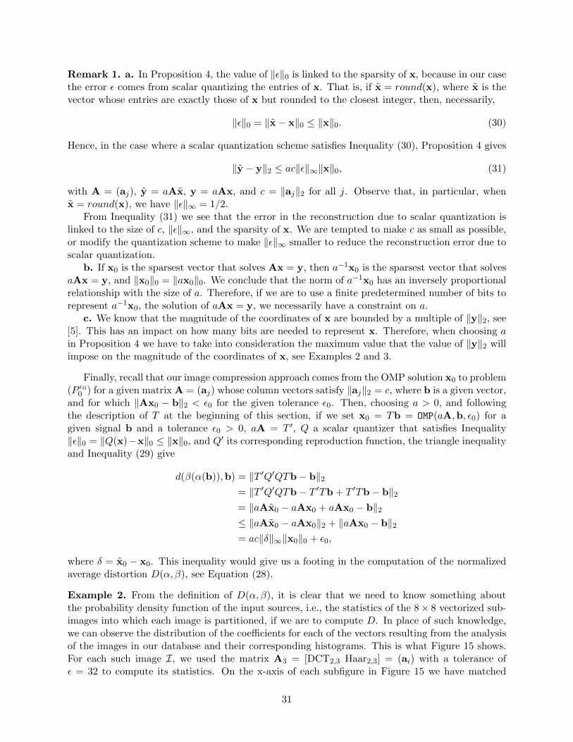
Example 4. In Figure 17, we have plotted the distortion as measured by both the MSSIM indexand the PSNR versus the idealized normalized sparse bit-rate. This bit-rate is unattainable inpractice but nonetheless gives us an idea of an upper bound in the rate-distortion trade-off. Italso allows us to compare how much room we have to select a lossless encoder γ to completethe implementation of a quantizer using our sparse image representation approach. Figure 18(a)shows the PSNR versus normalized sparse bit-rate trade-off for image Lena, that we computed tocompare with Figure 18(b), which shows results for that image for three published fully implemented

32

(a) (b)

Figure 18: PSNR vs bit-rate: (a) Normalized sparse bit-rate results for A = [DCT1 Haar1] priorto any γ coding, and (b) bit-rate coding performances published in [33] for image Lena: Saidand Pearlman’s SPIHT algorithm [34], Embeded Coding and the Wavelet-Difference-Reductioncompression algorithm (“new algorithm”) [39], and Shapiro’s EZW algorithm [37].

quantizers. We observe that there is enough room to pick an encoder γ that could compete withthese implementations.

Regarding the computation of the rate R(α, γ) for our image quantizer, we would have to choosea lossless encoder γ, which we have not done here.

10 Acknowledgement

The first named author gratefully acknowledges the support of MURI-ARO Grant W911NF-09-1-0383, NGA Grant 1582-08-1-0009, and DTRA Grant HDTRA1-13-1-0015. The second namedauthor gratefully acknowledges the support of the Institute for Physical Science and Technologyat the University of Maryland, College Park. We are both appreciative of expert observationsby Professor Radu V. Balan, Department of Mathematics and Center for Scientific Computationand Mathematical Modeling (CSCAMM), Professor Ramani Duraiswami, Department of ComputerScience and University of Maryland Institute of Advanced Computer Studies (UMIACS), and Pro-fessor Wojciech Czaja, Department of Mathematics, all at the University of Maryland, CollegePark.

References

[1] Enrico Au-Yeung and John J. Benedetto. Balayage and short time Fourier transform frames.Proceedings of SampTA, 2013.

[2] David Austin. What is... JPEG? Notices of the AMS, 55(2):226–229, February 2008.

[3] John J. Benedetto. Harmonic Analysis and Applications. CRC Press, Boca Raton, FL, 1997.

33

[4] John J. Benedetto and M. W. Frazier. Wavelets: Mathematics and Applications. CRC Press,Boca Raton, FL, 1994.

[5] John J. Benedetto and Alfredo Nava-Tudela. Frame estimates for OMP. Preprint, 2014.

[6] John J. Benedetto, Alex M. Powell, and O. Yilmaz. Sigma-delta (Σ∆) quantization and finiteframes. IEEE Transactions on Information Theory, 52(5):1990–2005, May 2006.

[7] Arne Beurling. The Collected Works of Arne Beurling. Vol. 2. Harmonic Analysis. Birkhauser,Boston, 1989.

[8] Arne Beurling and Paul Malliavin. On Fourier transforms of measures with compact support.Acta Mathematica, 107:291–309, 1962.

[9] Arne Beurling and Paul Malliavin. On the closure of characters and the zeros of entire func-tions. Acta Mathematica, 118:79–93, 1967.

[10] William L. Briggs and Van Emden Henson. The DFT, an Owner’s Manual for the DiscreteFourier Transform. SIAM, Philadelphia, PA, 1995.

[11] Alfred M. Bruckstein, David L. Donoho, and Michael Elad. From sparse solutions of systemsof equations to sparse modeling of signals and images. SIAM Review, 51(1):34–81, 2009.

[12] James C. Candy and Gabor C. Temes, editors. Oversampling Delta-Sigma Data Converters.IEEE Press, NY, 1992.

[13] Peter G. Casazza and J. Kovacevic. Uniform tight frames with erasures. Advances in Compu-tational Mathematics, 18(2-4):387–430, February 2003.

[14] Ole Christensen. An Introduction to Frames and Riesz Bases. Springer-Birkhauser, NY, 2003.

[15] Charilaos Christopoulos, Athanassios Skodras, and Touradj Ebrahimi. The JPEG 2000 stillimage coding system: an overview. IEEE Transactions on Consumer Electronics, 46(4):1103–1127, November 2000.

[16] David Donoho, Iain Johnstone, Peter Rousseeuw, and Werner Stahel. Discussion: Projectionpursuit. Annals of Statistics, 13(2):496–500, June 1985.

[17] Richard J. Duffin and A. C. Schaeffer. A class of nonharmonic Fourier series. Trans. Amer.Math. Soc., 72:341–366, 1952.

[18] James Gleick. The Information: a History, a Theory, a Flood. Pantheon Books, New York,NY, 2011.

[19] Robert M. Gray and David L. Neuhoff. Quantization. IEEE Transactions on InformationTheory, 44(6):2325–2383, October 1998.

[20] Karlheinz Grochenig. Foundations of Time-Frequency Analysis. Applied and Numerical Har-monic Analysis. Birkhauser Boston Inc., Boston, MA, 2001.

[21] Matthew A. Herman and Thomas Strohmer. High-resolution radar via compressed sensing.IEEE Transactions on Signal Processing, 57(6):2275–2284, June 2009.

[22] Peter J. Huber. Projection pursuit. Annals of Statistics, 13(2):435–475, June 1985.

34

[23] W. Cary Huffman and Vera Pless. Fundamentals of Error-Correcting Codes. CambridgeUniversity Press, New York, NY, 2010.

[24] Stephane Jaffard. A density criterion for frames of complex exponentials. Michigan Math. J.,38:339–348, 1991.

[25] Henry J. Landau. Necessary density conditions for sampling and interpolation of certain entirefunctions. Acta Mathematica, 117:37–52, 1967.

[26] Stephane G. Mallat. A Wavelet Tour of Signal Processing. Academic Press, San Diego, CA,1998.

[27] Stephane G. Mallat and Zhifeng Zhang. Matching pursuits with time-frequency dictionaries.IEEE Transactions on Signal Processing, 41(12):3397–3415, December 1993.

[28] Balas Kausik Natarajan. Sparse approximate solutions to linear systems. SIAM Journal onComputing, 24(2):227–234, 1995.

[29] Y. Pati, R. Rezaiifar, and P. Krishnaprasad. Orthogonal matching pursuit: recursive functionapproximation with application to wavelet decomposition. In 27th Asilomar Conference onSignals, Systems and Computers, 1993, pages 40–44, 1993.

[30] Gotz E. Pfander. Gabor frames in finite dimensions. In Peter G. Casazza and Gitta Kutyniok,editors, Finite Frames: Theory and Applications, pages 193–239. Birkhauser, 2013.

[31] Vera S. Pless and W. Cary Huffman, editors. Handbook of Coding Theory, volume 1. ElsevierScience B. V., Amsterdam, The Netherlands, 1998.

[32] K. R. Rao and P. Yip. Discrete Cosine Transform: Algorithms, Advantages, Applications.Academic Press Professional, Inc., San Diego, CA, USA, 1990.

[33] Howard L. Resnikoff and Raymond O. Wells, Jr. Wavelet Analysis. The Scalable Structure ofInformation. Springer-Verlag, New York, NY, 1998. Corrected 2nd printing.

[34] A. Said and W. A. Pearlman. A new, fast, and efficient image codec based on set partitioning inhierarchical trees. IEEE Transactions on Circuits and Systems for Video Technology, 6(3):243–250, June 1996.

[35] K. Seip. On the connection between exponential bases and certain related sequences inL2(−π, π). J. Funct. Anal., 130:131–160, 1995.

[36] Claude E. Shannon. A mathematical theory of communication. The Bell System TechnicalJournal, 27:379–423, 623–656, July, October 1948.

[37] Jerome M. Shapiro. Embedded image coding using zerotrees of wavelet coefficients. IEEETransactions on Signal Processing, 41(12):3445–3462, December 1993.

[38] D. S. Taubman and Michael W. Marcellin. JPEG 2000: Image Compression Fundamentals,Standards and Practice. Kluwer Academic Publishers, Norwell, MA, second edition, 2002.

[39] J. Tian and R. O. Wells, Jr. A lossy image codec based on index coding. In IEEE DataCompression Conference, DCC ’96, page 456, 1996.

35

[40] Viterbi School of Engineering, University of Southern California. The USC-SIPI ImageDatabase. http://sipi.usc.edu/database/, 2012.

[41] Gregory K. Wallace. The JPEG still picture compression standard. Communications of theACM, 34(4):30–44, 1991.

[42] Zhou Wang, Alan C. Bovik, Hamid R. Sheikh, and Eero P. Simoncelli. Image quality as-sessment: From error measurement to structural similarity. IEEE Transactions on ImageProcessing, 13(1):1–14, 2004.

[43] Andrew B. Watson, editor. Digital Images and Human Vision. MIT Press, Cambridge, MA,1993.

[44] Mladen V. Wickerhauser. Adapted Wavelet Analysis from Theory to Software. A K Peters,Ltd., 1996.

36