Sampling Effect on Performance Prediction of Configurable ...

HAL Id: hal-02356290https://hal.inria.fr/hal-02356290v2

Submitted on 26 Feb 2020 (v2), last revised 21 Apr 2020 (v3)

HAL is a multi-disciplinary open accessarchive for the deposit and dissemination of sci-entific research documents, whether they are pub-lished or not. The documents may come fromteaching and research institutions in France orabroad, or from public or private research centers.

L’archive ouverte pluridisciplinaire HAL, estdestinée au dépôt et à la diffusion de documentsscientifiques de niveau recherche, publiés ou non,émanant des établissements d’enseignement et derecherche français ou étrangers, des laboratoirespublics ou privés.

Sampling Effect on Performance Prediction ofConfigurable Systems: A Case Study

Juliana Alves Pereira, Mathieu Acher, Hugo Martin, Jean-Marc Jézéquel

To cite this version:Juliana Alves Pereira, Mathieu Acher, Hugo Martin, Jean-Marc Jézéquel. Sampling Effect on Perfor-mance Prediction of Configurable Systems: A Case Study. International Conference on PerformanceEngineering, ACM, Apr 2020, Edmonton, Canada. �hal-02356290v2�

https://hal.inria.fr/hal-02356290v2

https://hal.archives-ouvertes.fr

Sampling Effect on Performance Prediction ofConfigurable Systems: A Case Study

JULIANA ALVES PEREIRA, Univ Rennes, Inria, CNRS, IRISA

MATHIEU ACHER, Univ Rennes, Inria, CNRS, IRISA

HUGO MARTIN, Univ Rennes, Inria, CNRS, IRISA

JEAN-MARC JÉZÉQUEL, Univ Rennes, Inria, CNRS, IRISA

Numerous software systems are highly configurable and provide a myriad of configuration options that users can tune to fit theirfunctional and performance requirements (e.g., execution time). Measuring all configurations of a system is the most obvious wayto understand the effect of options and their interactions, but is too costly or infeasible in practice. Numerous works thus proposeto measure only a few configurations (a sample) to learn and predict the performance of any combination of options’ values. Achallenging issue is to sample a small and representative set of configurations that leads to a good accuracy of performance predictionmodels. A recent study devised a new algorithm, called distance-based sampling, that obtains state-of-the-art accurate performancepredictions on different subject systems. In this paper, we replicate this study through an in-depth analysis of x264, a popular andconfigurable video encoder. We systematically measure all 1,152 configurations of x264 with 17 input videos and two quantitativeproperties (encoding time and encoding size). Our goal is to understand whether there is a dominant sampling strategy over the verysame subject system (x264), i.e., whatever the workload and targeted performance properties. The findings from this study show thatrandom sampling leads to more accurate performance models. However, without considering random, there is no single “dominant"sampling, instead different strategies perform best on different inputs and non-functional properties, further challenging practitionersand researchers.

Additional Key Words and Phrases: Software Product Lines, Configurable Systems, Machine Learning, Performance Prediction

1 INTRODUCTION

Configurable software systems offer a multitude of configuration options that can be combined to tailor the systems’functional behavior and performance (e.g., execution time, memory consumption). Options often have a significantinfluence on performance properties that are hard to know and model a priori. There are numerous possible optionsvalues, logical constraints between options, and subtle interactions among options [15, 25, 46, 51, 52] that can have aneffect while quantitative properties such as execution time are themselves challenging to comprehend.

Measuring all configurations of a configurable system is the most obvious path to e.g., find a well-suited configuration,but is too costly or infeasible in practice. Machine-learning techniques address this issue by measuring only a subset ofconfigurations (known as sample) and then using these configurations’ measurements to build a performance modelcapable of predicting the performance of other configurations (i.e., configurations not measured before). Several worksthus follow a "sampling, measuring, learning" process [3, 15, 20–23, 27, 40, 42, 43, 46, 51, 52, 60, 63, 64]. A crucial step isthe way the sampling is realized, since it can drastically affect the performance model accuracy [25, 46]. Ideally, thesample should be small to reduce the cost of measurements and representative of the configuration space to reduceprediction errors. The sampling phase involves a number of difficult activities: (1) picking configurations that arevalid and conform to constraints among options – one needs to resolve a satisfiability problem; (2) instrumenting theexecutions and observations of software for a variety of configurations – it might have a high computational costespecially when measuring performance aspects of software; (3) guaranteeing a coverage of the configuration space toobtain a representative sample set. An ideal coverage includes all influential configuration options by covering different

1

ICPE ’20, April 20–24, 2020, Edmonton, AB, Canada Juliana Alves Pereira, Mathieu Acher, Hugo Martin, and Jean-Marc Jézéquel

kinds of interactions relevant to performance. Otherwise, the learning may hardly generalize to the whole configurationspace.

With the promise to select a small and representative sample set of valid configurations, several sampling strategieshave been devised in the last years [46]. For example, random sampling aims to cover the configuration space uniformlywhile coverage-oriented sampling selects the sample set according to a coverage criterion (e.g., t-wise sampling to coverall combinations of t selected options). Recently, Kaltenecker et al. [25] analyzed 10 popular real-world software systemsand found that their novel proposed sampling strategy, called diversified distance-based sampling, dominates five othersampling strategies by decreasing the cost of labelling software configurations while minimizing the prediction errors.

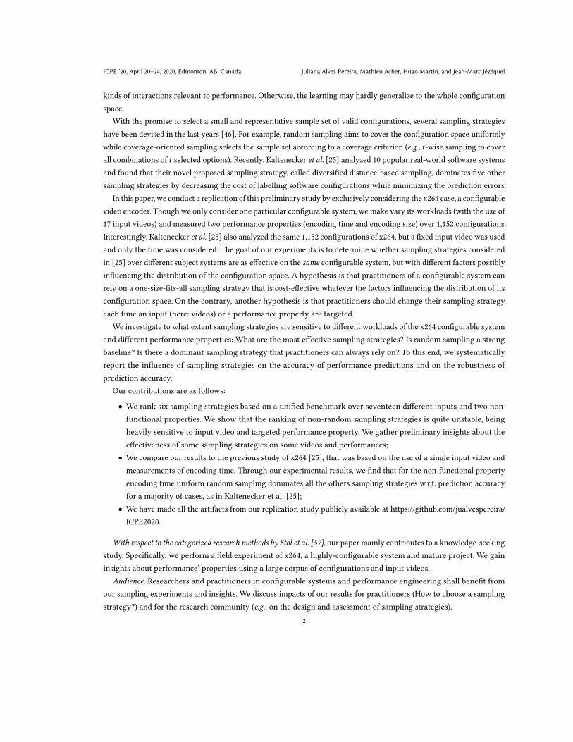
In this paper, we conduct a replication of this preliminary study by exclusively considering the x264 case, a configurablevideo encoder. Though we only consider one particular configurable system, we make vary its workloads (with the use of17 input videos) and measured two performance properties (encoding time and encoding size) over 1,152 configurations.Interestingly, Kaltenecker et al. [25] also analyzed the same 1,152 configurations of x264, but a fixed input video was usedand only the time was considered. The goal of our experiments is to determine whether sampling strategies consideredin [25] over different subject systems are as effective on the same configurable system, but with different factors possiblyinfluencing the distribution of the configuration space. A hypothesis is that practitioners of a configurable system canrely on a one-size-fits-all sampling strategy that is cost-effective whatever the factors influencing the distribution of itsconfiguration space. On the contrary, another hypothesis is that practitioners should change their sampling strategyeach time an input (here: videos) or a performance property are targeted.

We investigate to what extent sampling strategies are sensitive to different workloads of the x264 configurable systemand different performance properties: What are the most effective sampling strategies? Is random sampling a strongbaseline? Is there a dominant sampling strategy that practitioners can always rely on? To this end, we systematicallyreport the influence of sampling strategies on the accuracy of performance predictions and on the robustness ofprediction accuracy.

Our contributions are as follows:

• We rank six sampling strategies based on a unified benchmark over seventeen different inputs and two non-functional properties. We show that the ranking of non-random sampling strategies is quite unstable, beingheavily sensitive to input video and targeted performance property. We gather preliminary insights about theeffectiveness of some sampling strategies on some videos and performances;

• We compare our results to the previous study of x264 [25], that was based on the use of a single input video andmeasurements of encoding time. Through our experimental results, we find that for the non-functional propertyencoding time uniform random sampling dominates all the others sampling strategies w.r.t. prediction accuracyfor a majority of cases, as in Kaltenecker et al. [25];

• We have made all the artifacts from our replication study publicly available at https://github.com/jualvespereira/ICPE2020.

With respect to the categorized research methods by Stol et al. [57], our paper mainly contributes to a knowledge-seekingstudy. Specifically, we perform a field experiment of x264, a highly-configurable system and mature project. We gaininsights about performance’ properties using a large corpus of configurations and input videos.

Audience. Researchers and practitioners in configurable systems and performance engineering shall benefit fromour sampling experiments and insights. We discuss impacts of our results for practitioners (How to choose a samplingstrategy?) and for the research community (e.g., on the design and assessment of sampling strategies).

2

https://github.com/jualvespereira/ICPE2020

https://github.com/jualvespereira/ICPE2020

Sampling Effect on Performance Prediction ofConfigurable Systems: A Case Study ICPE ’20, April 20–24, 2020, Edmonton, AB, Canada

Sampling configurations

x264 --no-cabac --no-fast-pskip --ref 9 -o video0.264 video0.y4m

Measuringconfigurations

Learning

Performanceprediction

model

video1

video0

video16

…

(configuration sample aka training set)

prediction errors (MRE)

random distance-based

coverage-based

Input videos

(workload)

What is the influence of a sampling strategy, over different workloads and performance properties of x264, on the

accuracy of performance predictions and on the robustness of prediction accuracy?

(on the same hardware)

(x264 version is the same for all experiments)

…

Fig. 1. Design study: sampling effect on performance predictions of x264 configurations

2 BACKGROUND AND RELATEDWORK

In this section, we introduce basic concepts of configurable software systems and motivate the use of learning techniquesin this field. Furthermore, we briefly describe six state-of-the-art sampling strategies used in our experiments.

2.1 Learning Software Configuration Spaces

x264 is a command-line tool to encode video streams into the H.264/MPEG-4 AVC format. Users can configure x264through the selection of numerous options, some having an effect on the time needed to encode a video, on the qualityor the size of the output video, etc. A configuration of x264 is an assignment of values to options. In our study andas in [25], we only consider Boolean options that can be selected or deselected. As in most configurable systems, notall combinations of options are valid due to constraints among options. For instance, ref_1, ref_5, and ref_9 aremutually exclusive and at least one of these options should be selected.

Executing and measuring every valid configuration to know about its performance or identify the performance-optimal one is often unfeasible or costly. To overcome this problem, machine learning techniques rely on a small andrepresentative sample of configurations (see Figure 1). Each configuration of the sample is executed and labelled witha performance measurement (e.g., encoding time). The sample is then used for training a learning algorithm (i.e., aregressor) that builds a performance model capable of predicting the performance of unmeasured configurations. Theperformance model may lead to prediction errors. The overall goal is to obtain high accuracy roughly computed asthe difference between actual performances and predicted performances (more details are given hereafter). How toefficiently sample, measure, and learn is subject to intensive research [46]. In case important (interactions among)options are not included in the training set, the learning phase can hardly generalize to the whole population ofconfigurations. Hence, sampling is a crucial step of the overall learning process with an effect on the accuracy of theprediction model.

2.2 Sampling Strategies

Several sampling strategies have been proposed in the literature about software product lines and configurable sys-tems [46, 62, 66].

3


Sampling for testing. Some works consider sampling for the specific case of testing configurations. There is notnecessarily a learning phase and the goal of sampling is mostly to find and cover as many faults as possible. For instance,Medeiros et al. compared 10 sampling algorithms to detect different faults in configurable systems [35]. Arcuri et al.theoretically demonstrate that a uniform random sampling strategy may outperform coverage-based sampling [5](see hereafter). Halin et al. demonstrated that uniform random sampling forms a strong baseline for faults and failureefficiency on the JHipster case [17]. Varshosaz et al. [66] conducted a survey of sampling for testing configurablesystems. Though the purpose differs, some of these sampling strategies are also relevant and considered in the contextof performance prediction.

Sampling for learning. Pereira et al. [46] review several sampling strategies specifically used for learning configurationspaces. We now present an overview of six sampling strategies also considered in [25] and used in our study. Allstrategies have the merit of being agnostic of the domain (no specific knowledge or prior analysis are needed) and aredirectly applicable to any configurable system.

Random sampling aims to cover the configuration space uniformly. Throughout the paper, we refer to random asuniform random sampling. The challenge is to select one configuration amongst all the valid ones in such a way eachconfiguration receives an equal probability to be included in the sample. An obvious solution is to enumerate all validconfigurations .and randomly pick a sample from the whole population. However, enumerative approaches quickly donot scale with a large number of configurations. Oh et al. [43] rely on binary decision diagrams to compactly represent aconfiguration space, which may not scale for very large systems [36]. Another line of research is to rely on satisfiability(SAT) solvers. For instance, UniGen [8, 9] uses a hashing-based functions to synthesize samples in a nearly uniformmanner with strong theoretical guarantees. These theoretical properties come at a cost: the hashing-based approachrequires adding large clauses to formulas. Plazar et al. [47] showed that state-of-the-art algorithms are either not ableto produce any sample or unable to generate uniform samples for the SAT instances considered. Overall, a true uniformrandom sampling may be hard to realize, especially for large configurable systems. At the scale of the x264 study [25],though, uniform sampling is possible (the whole population is 1,152 configurations). The specific question we explorehere is whether random is effective for learning (in case it is applicable as in x264).

When random sampling is not applicable, several alternate techniques have been proposed typically by sacrificingsome uniformity for a substantial increase in performance.

Solver-based. Many works rely on off-the-shelf constraint solver, such as SAT4J [31] or Z3 [12], for sampling. Forinstance, a random seed can be set to the Z3 solver and internally influences the variable selection heuristics, whichcan have an effect on the exploration of valid configurations. Henard et al. noticed that solvers’ internal order yieldsnon-uniform (and predictable) exploration of the configuration space [18]. Hence, these strategies do not guarantee truerandomness as in uniform random sampling. Often the sample set consists of a locally clustered set of configurations.

Randomized solver-based. To weaken the locality drawback of solver-based sampling, Henard et al. change the orderof variables and constraints at each solver run. This strategy, called randomized solver-based sampling in Kaltenecker etal. [25], increases diversity of configurations. Though it cannot give any guarantees about randomness, the diversitymay help to capture important interactions between options for performance prediction.

Coverage-based sampling aims to optimize the sample with regards to a coverage criterion. Many criteria can beconsidered such as statement coverage that requires the analysis of the source code. In this paper and as in Kaltenecker etal. [25], we rely on t-wise sampling [11, 24, 30]. This sampling strategy selects configurations to cover all combinations

4


of t selected options. For instance, pair-wise (t=2) sampling covers all pairwise combinations of options being selected.There are different methods to compute t-wise sampling. As in [25], we rely on the implementation of Siegmund et

al. [53].

Distance-based. Kaltenecker et al. [25] propose distance-based sampling. The idea is to cover the configuration spaceby selecting configurations according to a given probability distribution (typically a uniform distribution) and a distancemetric. The underlying benefit is that distance-based sampling can better scale compared to an enumerative-basedrandom sampling, while the generated samples are closed to those obtained with a uniform random.

Diversified distance-based sampling is a variant of distance-based sampling [25]. The principle is to increase diversityof the sample set by iteratively adding configurations that contain the least frequently selected options. The intendedbenefit is to avoid missing the inclusion of some (important) options in the process.

2.3 Sampling Effect on x264

This paper aims to replicate the study of Kaltenecker et al. [25]. While Kaltenecker et al. analyse a wide variety ofsystems from different domains, we focus on the analysis of a single configurable system. Compared to that paper,our study enables a deeper analysis of sampling strategies over the possible influences of inputs and performanceproperties. Specifically, we analyze a set of seventeen input videos and two non-functional properties. As in [25],we collect results of 100 independent experiments to increase statistical confidence and external validity. We aim atexploring whether the results obtained in [25] may be generalized over different variations of a single configurablesystem. Interestingly, numerous papers have specifically considered the x264 configurable system for assessing theirproposals [15, 21, 22, 43, 46, 51, 58, 63, 64], but a fixed performance property or input video is usually considered.Jamshidi et al. [21] explore the impacts of versions, workloads, and hardware of several configurable systems, includingx264. However, the effect of sampling strategies was not considered. In [22], sampling strategies for transfer learningwere investigated; we are not considering such scenarios in our study. Overall, given a configurable system like x264,practitioners face the problem of choosing the right techniques for "sampling, measuring, learning". Specifically, weaim to understand what sampling strategy to use and whether there exists a sampling to rule any configuration spaceof x264.

The use of different input videos obviously changes the raw and absolute performance values, but it can also changethe overall distribution of configuration measurements. Figure 2 gives two distributions over two input videos forthe performance property size for the whole population of valid configurations. Pearson correlation between theperformance measurements of x2642 and x26415 is -0.35, suggesting a weak, negative correlation. The differencesamong distributions question the existence of a one-size-fits-all sampling capable of generating a representative sampleset whatever the input videos or performance properties. Another hypothesis is that the way the sampling is done canpay off for some distributions but not for all.

Given the vast variety of possible input videos and performance properties that may be considered, the performancevariability of configurations grows even more. Our aim is to investigate how such factors affect the overall predictionaccuracy of different sampling strategies: Is there a dominant sampling strategy for performance prediction of the same

configurable system?

3 DESIGN STUDY

In this section, we introduce our research questions, the considered subject system, and the experiment setup.5


0.70 0.75 0.80 0.85 0.90 0.95 1.00 1.05Video size (bytes) 1e7

0

5

10

15

20

25

30

35

40

Freq

uenc

y

(a) flower_sif.y4m x2642

0.8 1.0 1.2 1.4 1.6 1.8Video size (bytes) 1e7

0

20

40

60

80

100

Freq

uenc

y

(b) 720p50_parkrun_ter.y4m x26415Fig. 2. The size distribution of 1,152 configurations of x264 over two input videos

3.1 ResearchQuestions

We conducted a series of experiments to evaluate six sampling strategies and to compare our results to the originalresults in [25]. We aim at answering the following two research questions:

• (RQ1) What is the influence of using different sampling strategies on the accuracy of performance predictionsover different inputs and non-functional properties?

• (RQ2)What is the influence of randomness of using different sampling strategies on the robustness of predictionaccuracy?

It is not new the claim that the prediction accuracy of machine learning extensively depends on the samplingstrategy. The originality of the research question is to what extent are performance prediction models of the same

configurable system (here: x264) sensitive to other factors, such as different inputs and non-functional properties. Toaddress RQ1, we analyze the sensitivity of the prediction accuracy of sampling strategies to these factors. Since mostof the considered sampling strategies use randomness, which may considerably affect the prediction accuracy, RQ2quantitatively compares whether the variances (over 100 runs) on prediction accuracy between different samplingstrategies and sample sizes differ significantly. We show that the sampling prediction accuracy and robustness hardlydepends on the definition of performance (i.e., encoding time or encoding size). As in Kaltenecker et al. [25], we haveexcluded t-wise sampling from RQ2, as it is also deterministic in our setting and does not lead to variations.

3.2 Subject System

We conduct an in-depth study of x264, a popular and highly configurable video encoder implemented in C. We choosex264 instead of the other case studies documented in Kaltenecker et al. [25] because x264 demonstrated more promisingaccuracy results to the newest proposed sampling approach (i.e., diversified distance-based sampling). With this study,we aim at investigating, for instance, whether diversified distance-based sampling also dominates across differentvariations of x264 (i.e., inputs, performance properties). As benchmark, we encoded 17 different input videos from rawYUV to the H.264 codec and measured two quantitative properties (encoding time and encoding size).

• Encoding time (in short time): how many seconds x264 takes to encode a video.• Encoding size of the output video (in short size): compression size (in bytes) of an output video in the H.264format.

6


video #times stability

x2640 bridge_far_cif.y4m 5 0.010127x2641 ice_cif.y4m 5 0.044476x2642 flower_sif.y4m 5 0.036826x2643 claire_qcif.y4m 5 0.086958x2644 sintel_trailer_2k_480p24.y4m 9 0.009481x2645 football_cif.y4m 5 0.029640x2646 crowd_run_1080p50.y4m 3 0.005503x2647 blue_sky_1080p25.y4m 8 0.010468x2648 FourPeople_1280x720_60.y4m 11 0.011258x2649 sunflower_1080p25.y4m 4 0.006066x26410 deadline_cif.y4m 23 0.014536x26411 bridge_close_cif.y4m 5 0.009892x26412 husky_cif.y4m 5 0.028564x26413 tennis_sif.y4m 5 0.044731x26414 riverbed_1080p25.y4m 3 0.007625x26415 720p50_parkrun_ter.y4m 8 0.010531x26416 soccer_4cif.y4m 16 0.011847

Table 1. Overview of encoded input videos including the number of times we measured the encoding time in order to ensure we havea stable set of measurements (according to RSD results), independent of the machine.

All measurements have been performed over the same version of x264 and on a grid computing infrastructure calledIGRIDA1. Importantly, we used the same hardware characteristics for all performance measurements. In Table 1, weprovide an overview of the encoded input videos. This number of inputs allows us to draw conclusions about thepracticality of sampling strategies for diversified conditions of x264.

To control measurement bias while measuring execution time, we have repeated the measurements several times. Wereport in Table 1 how many times we have repeated the time measurements of all 1,152 configurations for each videoinput. the number of repetitions has been increased to reach a standard deviation of less than 10%. Since measurementsare costly, we set the repetition to up 30 times given 1-hour restriction from where we got the #times in Table 1. Werepeated the measurements at least three times and at most 23 times and retained the average execution time foreach configuration. The stability column reports whether the configuration measurements for a given input videoare stable (Relative Standard Deviation - RSD). For example, measurements have been repeated 5 times for video0 (bridge_far_cif.y4m) and the measurements present low RSD of ≈ 1%. Although the RSD measure for Video 3(claire_qcif.y4m) is higher compared to the others, the deviation still remains lower than 10% (i.e., RSD ≈ 8.7%). Weprovide the variability model and the measurements of each video input for encoding time and encoding size on oursupplementary website.

3.3 Experiment Setup

In our experiments, the independent variables are the choice of the input videos, the predicted non-functional-property,the sample strategies and the sample sizes.

For comparison, we used the same experiment design than in Kaltenecker et al. [25]. To evaluate the accuracy ofdifferent sampling strategies over different inputs and non-functional-properties, we conducted experiments usingthree different sample sizes. To be able to use the same sample sizes for all sampling strategies, we consider the sizes1http://igrida.gforge.inria.fr/

7

http://igrida.gforge.inria.fr/


Video Coverage-based Solver-based Randomized solver-based Distance-based Diversified distance-based Random

t = 1 t = 2 t = 3 t = 1 t = 2 t = 3 t = 1 t = 2 t = 3 t = 1 t = 2 t = 3 t = 1 t = 2 t = 3 t = 1 t = 2 t = 3

x2640 18.2 % 13.9 % 13.4 % 24.0 % 27.0 % 27.5 % 22.3 % 19.9 % 24.3 % 16.5 % 12.7 % 10.6 % 16.3 % 8.8 % 8.2 % 16.7 % 9.2 % 8.2 %

x2641 15.4 % 13.2 % 12.1 % 26.9 % 23.7 % 24.9 % 21.4 % 21.5 % 23.2 % 17.3 % 14.2 % 9.5 % 17.4 % 9.8 % 8.7 % 16.1 % 9.2 % 8.7 %

x2642 29.3 % 10.3 % 9.7 % 21.4 % 19.4 % 16.4 % 19.1 % 19.6 % 19.4 % 17.4 % 11.4 % 9.8 % 17.6 % 9.6 % 9.3 % 15.3 % 9.5 % 9.3 %

x2643 21.4 % 13.7 % 10.1 % 25.2 % 25.3 % 26.4 % 16.4 % 22.3 % 24.8 % 13.6 % 10.7 % 10.2 % 12.8 % 9.8 % 9.7 % 14.5 % 9.8 % 9.2 %

x2644 21.8 % 12.3 % 14.4 % 23.9 % 21.2 % 22.0 % 18.3 % 21.1 % 22.5 % 14.2 % 11.7 % 9.7 % 13.9 % 10.1 % 8.9 % 13.9 % 9.4 % 8.8 %

x2645 26.1 % 14.1 % 13.2 % 28.8 % 23.2 % 24.1 % 21.8 % 22.5 % 23.3 % 16.4 % 13.4 % 11.4 % 16.8 % 10.7 % 9.5 % 15.7 % 10.0 % 9.3 %

x2646 25.9 % 18.1 % 8.6 % 23.6 % 28.5 % 29.1 % 18.2 % 21.6 % 24.9 % 13.7 % 9.9 % 9.0 % 13.2 % 8.8 % 7.8 % 12.6 % 8.0 % 7.3 %

x2647 23.3 % 14.2 % 12.0 % 20.2 % 25.3 % 26.1 % 15.3 % 23.0 % 23.8 % 12.2 % 9.2 % 7.2 % 10.8 % 8.5 % 7.2 % 11.4 % 8.2 % 7.3 %

x2648 20.8 % 13.1 % 11.5 % 20.3 % 22.7 % 23.6 % 16.7 % 23.4 % 23.4 % 12.6 % 10.4 % 9.6 % 11.1 % 9.3 % 8.3 % 12.0 % 8.7 % 7.6 %

x2649 23.4 % 13.2 % 5.6 % 22.1 % 28.6 % 29.7 % 16.8 % 24.2 % 25.3 % 11.4 % 6.5 % 6.5 % 9.2 % 5.8 % 5.4 % 10.9 % 6.6 % 5.4 %

x26410 21.9 % 12.3 % 9.3 % 22.6 % 23.2 % 24.0 % 17.9 % 22.4 % 24.3 % 14.0 % 10.2 % 9.7 % 13.5 % 9.4 % 8.9 % 14.0 % 9.0 % 8.8 %

x26411 21.1 % 12.6 % 10.3 % 25.7 % 23.5 % 23.8 % 20.0 % 21.1 % 24.7 % 13.3 % 10.8 % 10.4 % 13.0 % 10.1 % 9.7 % 13.9 % 9.4 % 9.1 %

x26412 25.4 % 13.4 % 10.4 % 26.2 % 21.2 % 21.6 % 19.8 % 20.6 % 20.9 % 16.2 % 13.7 % 10.9 % 16.3 % 11.4 % 9.1 % 15.0 % 9.7 % 8.5 %

x26413 16.4 % 10.5 % 10.0 % 20.6 % 18.8 % 19.1 % 18.3 % 19.4 % 19.8 % 16.0 % 13.9 % 10.0 % 16.2 % 10.5 % 9.6 % 15.5 % 9.7 % 9.0 %

x26414 20.7 % 16.9 % 15.8 % 34.3 % 39.5 % 40.6 % 28.5 % 29.7 % 32.4 % 18.1 % 11.1 % 9.6 % 18.4 % 7.8 % 7.3 % 17.4 % 7.5 % 7.2 %

x26415 26.2 % 12.7 % 11.1 % 23.2 % 26.5 % 27.2 % 20.3 % 22.7 % 25.1 % 15.1 % 11.9 % 10.7 % 14.8 % 10.6 % 9.5 % 13.9 % 9.1 % 8.9 %

x26416 22.9 % 12.3 % 8.4 % 22.1 % 24.5 % 25.2 % 18.0 % 22.2 % 23.6 % 13.4 % 9.4 % 8.9 % 12.6 % 8.5 % 7.8 % 12.5 % 8.1 % 7.4 %

Mean 22.4 % 13.3 % 10.9 % 24.2 % 24.8 % 25.4 % 19.4 % 22.2 % 23.9 % 14.8 % 11.3 % 9.6 % 14.3 % 9.4 % 8.5 % 14.2 % 8.9 % 8.2 %

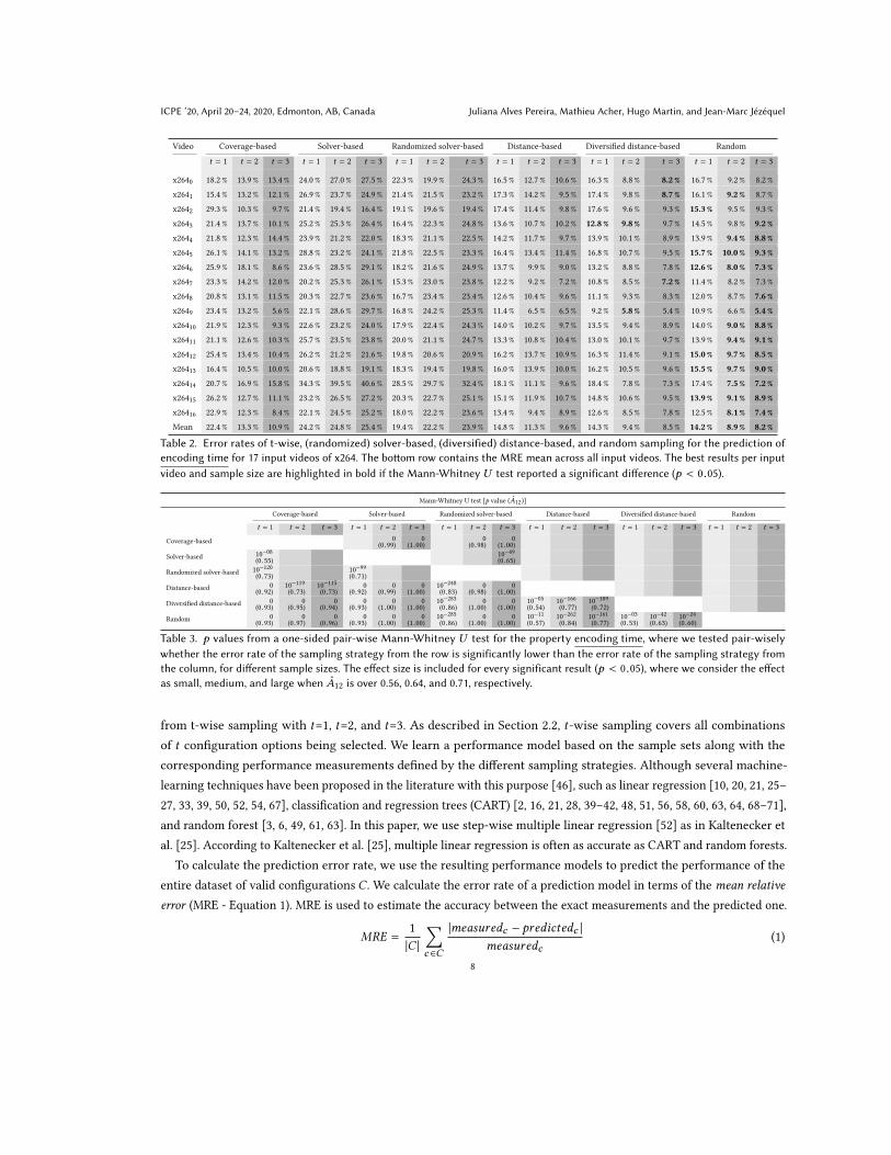
Table 2. Error rates of t-wise, (randomized) solver-based, (diversified) distance-based, and random sampling for the prediction ofencoding time for 17 input videos of x264. The bottom row contains the MRE mean across all input videos. The best results per inputvideo and sample size are highlighted in bold if the Mann-Whitney U test reported a significant difference (p < 0.05).

Mann-Whitney U test [p value (A12)]

Coverage-based Solver-based Randomized solver-based Distance-based Diversified distance-based Random

t = 1 t = 2 t = 3 t = 1 t = 2 t = 3 t = 1 t = 2 t = 3 t = 1 t = 2 t = 3 t = 1 t = 2 t = 3 t = 1 t = 2 t = 30 0 0 0Coverage-based (0.99) (1.00) (0.98) (1.00)

10−08 10−49Solver-based (0.55) (0.65)10−120 10−99Randomized solver-based (0.73) (0.71)

0 10−119 10−115 0 0 0 10−248 0 0Distance-based (0.92) (0.73) (0.73) (0.92) (0.99) (1.00) (0.83) (0.98) (1.00)0 0 0 0 0 0 10−283 0 0 10−05 10−166 10−109Diversified distance-based (0.93) (0.95) (0.94) (0.93) (1.00) (1.00) (0.86) (1.00) (1.00) (0.54) (0.77) (0.72)0 0 0 0 0 0 10−285 0 0 10−11 10−262 10−161 10−03 10−42 10−24Random (0.93) (0.97) (0.96) (0.93) (1.00) (1.00) (0.86) (1.00) (1.00) (0.57) (0.84) (0.77) (0.53) (0.63) (0.60)

Table 3. p values from a one-sided pair-wise Mann-Whitney U test for the property encoding time, where we tested pair-wiselywhether the error rate of the sampling strategy from the row is significantly lower than the error rate of the sampling strategy fromthe column, for different sample sizes. The effect size is included for every significant result (p < 0.05), where we consider the effectas small, medium, and large when A12 is over 0.56, 0.64, and 0.71, respectively.

from t-wise sampling with t=1, t=2, and t=3. As described in Section 2.2, t-wise sampling covers all combinationsof t configuration options being selected. We learn a performance model based on the sample sets along with thecorresponding performance measurements defined by the different sampling strategies. Although several machine-learning techniques have been proposed in the literature with this purpose [46], such as linear regression [10, 20, 21, 25–27, 33, 39, 50, 52, 54, 67], classification and regression trees (CART) [2, 16, 21, 28, 39–42, 48, 51, 56, 58, 60, 63, 64, 68–71],and random forest [3, 6, 49, 61, 63]. In this paper, we use step-wise multiple linear regression [52] as in Kaltenecker etal. [25]. According to Kaltenecker et al. [25], multiple linear regression is often as accurate as CART and random forests.

To calculate the prediction error rate, we use the resulting performance models to predict the performance of theentire dataset of valid configurations C . We calculate the error rate of a prediction model in terms of the mean relative

error (MRE - Equation 1). MRE is used to estimate the accuracy between the exact measurements and the predicted one.

MRE =1|C |

∑c ∈C

|measuredc − predictedc |

measuredc(1)

8


Where C is the set of all valid configurations used as the validation set, andmeasuredc and predictedc indicate themeasured and predicted values of performance for configuration c with c ∈ C , respectively. The exact value ofmeasuredc

is measured at runtime while running the configuration c , and the predicted values of predictedc is computed based onthe model built with a sample of configurations t (see Section 2.2). To address RQ1, we computed the mean error rate foreach input video and sample size. A lower error rate indicates a higher accuracy. Then, we use a Kruskal-Wallis test [29]and pair-wise one-sided Mann-Whitney U tests [34] to identify whether the error rate of two sampling strategiesdiffers significantly (p < 0.05) [4]. In addition, we compute the effect size A12 [65] (small(>0.56), medium(>0.64), andlarge(>0.71)) to easily compare the error rates of two sampling strategies.

To address RQ2, we compute the variance across the error rates over 100 runs. A lower variance indicates higherrobustness. First, we use Levene’s test [32] to identify whether the variances of two sampling strategies differ significantlyfrom each other. Then, for these sampling strategies, we perform a one-sided F-tests [55] to compare pair-wisely thevariance between sampling strategies.

All sampling and learning experiments have been performed on the same machine with Intel Core i7 CPU 2,2 GHzand 4GB RAM. To reduce fluctuations in the values of dependent variables caused by randomness (e.g., the randomgeneration of input samples), we evaluated each combination of the independent variables 100 times. That is, for eachinput video, non-functional property, sampling strategy and sampling size, we instantiated our experimental settingsand measured the values of all dependent variables 100 times with random seeds from 1 to 100.

4 RESULTS

We compare six sampling strategies: t-wise, solver-based, randomized solver-based, distance-based, diversified distance-based, and random. Next, we present the results regarding prediction accuracy (RQ1, Section 4.1) and robustness (RQ2,Section 4.2).

4.1 Results RQ1—Prediction Accuracy

In Tables 2 and 4, we show the MRE for the different sampling strategies and sample sizes for both encoding time andencoding size, respectively. In the bottom row, we provide the MRE mean over all input videos. As in Kaltenecker etal. [25], for each input video and sample-set size we highlight the lowest, statistically significant MRE in bold.

4.1.1 Input Sensitivity: Encoding Time. Random sampling performs best to all other sampling strategies or similar tothe best one for t=1, t=2 and t=3 (except for a few input videos – x2641, x2643, x2647, x2648, x2649, x26410, x26411 fort=1). We observe that for t=1 diversified distance-based sampling outperforms random sampling for seven input videos(x2640, x2643, x2647, x2648, x2649, x26410, x26411). Overall, diversified distance-based sampling produces partiallygood results (close to random sampling). Diversified distance-based sampling outperforms the pure distance basedsampling, however their error rates are very similar for t=1.

Solver-based sampling results in inaccurate performance models for all input videos and sample-set sizes. t-wisesampling performs overall better than solver-based sampling; randomized solver-based sampling performs best whenonly a very limited number of samples are considered (i.e., t=1).

Table 3 reports the p value (A12) of the Mann-Whitney U test. This table shows whether the sampling strategy ofthe row has a significantly lower error rate than the sampling strategy of the column. To this end, we first performedKruskal-Wallis tests for all sample sizes (t=1, t=2, and t=3). Then, whether we identified p values less than 0.05, indicating

9




x2640 12.3 % 11.6 % 11.1 % 12.3 % 11.4 % 11.3 % 25.1 % 12.7 % 13.3 % 25.3 % 12.5 % 10.6 % 23.3 % 10.6 % 9.2 % 13.1 % 9.8 % 9.1 %

x2641 4.0 % 3.9 % 3.8 % 3.1 % 3.8 % 3.8 % 1.7 % 3.8 % 3.8 % 4.0 % 4.0 % 3.8 % 3.9 % 3.8 % 3.8 % 3.9 % 3.8 % 3.8 %

x2642 14.9 % 14.3 % 4.8 % 5.1 % 4.7 % 4.7 % 15.9 % 4.7 % 4.6 % 14.3 % 14.0 % 10.2 % 13.8 % 12.0 % 4.7 % 7.6 % 4.7 % 4.6 %

x2643 8.6 % 8.3 % 7.8 % 8.1 % 7.3 % 7.4 % 11.2 % 7.6 % 7.4 % 9.9 % 9.3 % 8.0 % 9.6 % 8.3 % 7.5 % 7.7 % 7.4 % 7.3 %

x2644 18.4 % 16.7 % 6.6 % 4.5 % 6.8 % 6.8 % 14.1 % 6.7 % 6.7 % 17.5 % 16.7 % 7.0 % 16.9 % 6.9 % 6.9 % 7.8 % 6.9 % 6.9 %

x2645 11.3 % 11.0 % 10.8 % 4.9 % 6.6 % 5.7 % 12.3 % 9.4 % 4.8 % 11.8 % 11.5 % 10.9 % 11.6 % 10.6 % 10.0 % 9.4 % 6.4 % 5.2 %

x2646 24.6 % 5.3 % 5.2 % 5.4 % 5.4 % 5.3 % 25.6 % 5.3 % 5.3 % 17.6 % 16.8 % 5.5 % 16.1 % 5.4 % 5.4 % 6.3 % 5.3 % 5.3 %

x2647 9.4 % 9.0 % 8.7 % 8.1 % 8.4 % 8.3 % 8.4 % 8.2 % 8.2 % 9.4 % 9.4 % 8.9 % 9.3 % 8.6 % 8.5 % 9.1 % 8.4 % 8.3 %

x2648 10.4 % 9.7 % 8.9 % 8.7 % 8.0 % 8.1 % 11.2 % 7.6 % 8.0 % 12.4 % 12.0 % 9.5 % 12.0 % 9.9 % 8.5 % 8.5 % 8.3 % 8.2 %

x2649 11.6 % 10.5 % 9.5 % 7.6 % 8.6 % 8.5 % 6.9 % 8.4 % 8.4 % 11.3 % 11.6 % 9.6 % 10.8 % 9.7 % 8.7 % 8.8 % 8.5 % 8.4 %

x26410 5.2 % 5.2 % 4.9 % 5.2 % 5.0 % 4.8 % 5.0 % 4.6 % 4.6 % 6.0 % 5.8 % 5.0 % 5.7 % 5.1 % 4.7 % 4.9 % 4.6 % 4.6 %

x26411 12.4 % 11.8 % 11.1 % 11.1 % 10.8 % 11.0 % 8.8 % 9.9 % 11.4 % 12.8 % 11.8 % 9.0 % 12.0 % 10.2 % 8.6 % 10.9 % 9.4 % 8.8 %

x26412 25.7 % 3.6 % 3.6 % 5.3 % 3.5 % 3.6 % 28.9 % 3.6 % 3.5 % 16.5 % 14.6 % 3.5 % 15.4 % 3.5 % 3.4 % 4.8 % 3.5 % 3.4 %

x26413 4.7 % 4.7 % 4.6 % 4.5 % 4.7 % 4.7 % 5.4 % 4.8 % 4.7 % 5.1 % 5.0 % 4.8 % 5.0 % 4.7 % 4.7 % 5.0 % 4.7 % 4.6 %

x26414 10.2 % 9.6 % 9.4 % 5.1 % 7.4 % 8.8 % 3.6 % 9.6 % 9.5 % 10.6 % 10.6 % 10.0 % 9.8 % 9.6 % 9.6 % 9.3 % 9.0 % 9.5 %

x26415 4.1 % 4.0 % 4.0 % 7.5 % 4.5 % 4.3 % 40.9 % 4.3 % 4.2 % 21.7 % 8.3 % 4.1 % 19.1 % 4.1 % 4.1 % 5.4 % 4.2 % 4.1 %

x26416 8.3 % 8.1 % 7.9 % 7.7 % 7.8 % 7.6 % 9.2 % 7.7 % 7.6 % 8.8 % 8.7 % 8.2 % 8.7 % 7.9 % 7.7 % 8.3 % 7.7 % 7.6 %

Mean 11.5 % 8.7 % 7.2 % 6.7 % 6.8 % 6.7 % 13.8 % 7.0 % 6.8 % 12.6 % 10.7 % 7.6 % 12.0 % 7.7 % 6.8 % 7.7 % 6.6 % 6.5 %

Table 4. Error rates of t-wise, (randomized) solver-based, (diversified) distance-based, and random sampling for the prediction ofencoding size for 17 input videos of x264. The bottom row contains the MRE mean across all input videos. The best results per inputvideo and sample size are highlighted in bold if the Mann-Whitney U test reported a significant difference (p < 0.05).

Mann-Whitney U test [p value (A12)]

Coverage-based Solver-based Randomized solver-based Distance-based Diversified distance-based Random


0.01 10−33 10−176 10−78 10−08Coverage-based (0.52) (0.62) (0.78) (0.68) (0.55)10−232 10−268 10−43 10−152 10−247 0 10−145 10−219 10−86 10−95Solver-based (0.82) (0.85) (0.64) (0.76) (0.83) (0.92) (0.75) (0.81) (0.69) (0.70)

10−272 10−61 10−05 10−13 0 10−184 0.01 10−94 10−06Randomized solver-based (0.85) (0.66) (0.54) (0.57) (0.93) (0.79) (0.52) (0.70) (0.54)Distance-based

10−76 10−70 10−10 10−293 10−191Diversified distance-based (0.68) (0.68) (0.56) (0.86) (0.79)10−180 0 10−183 10−28 10−58 10−83 10−22 10−37 10−228 0 0 10−179 10−193 10−71Random (0.78) (0.92) (0.79) (0.61) (0.66) (0.69) (0.60) (0.63) (0.82) (0.96) (0.88) (0.78) (0.79) (0.68)

Table 5. p values from a one-sided pair-wise Mann-Whitney U test for the property encoding size, where we tested pair-wiselywhether the error rate of the sampling strategy from the row is significantly lower than the error rate of the sampling strategy fromthe column, for different sample sizes. The effect size is included for every significant result (p < 0.05), where we consider the effectas small, medium, and large when A12 is over 0.56, 0.64, and 0.71, respectively.

that, at least, two strategies differ significantly for each sample size [25], we performed one-sided Mann-WhitneyUtests pair-wisely and, if significant (p < 0.05), we report the effect sizes in Table 3.

The first row shows that t-wise sampling has significantly lower error rates than solver-based sampling andrandomized solver-based sampling for t=2 and t=3, with large effect sizes. In the second and third rows, we observethat solver-based sampling performs significantly better than randomized solver-based sampling for t=3 with mediumeffect sizes; and randomized solver-based leads to lower error rates than t-wise sampling for t=1, with a large effect size.In the last three rows, we see that (diversified) distance-based sampling and random sampling lead to lower error ratesthan t-wise sampling, solver-based sampling, and randomized solver-based sampling for t=1, t=2 and t=3, with largeeffect sizes.

The pure distance-based sampling leads to higher error rates than diversified distance-based sampling and randomsampling, for all sample sizes. However, comparing diversified distance-based sampling to random sampling, we see inthe last row that random sampling has significantly lower error rates with small effect sizes for all sample sizes. The

10


F-test (p value)

Solver-based Randomized solver-based Distance-based Diversified distance-based Random

t = 1 t = 2 t = 3 t = 1 t = 2 t = 3 t = 1 t = 2 t = 3 t = 1 t = 2 t = 3 t = 1 t = 2 t = 3Solver-basedRandomized solver-based 10−252 10−125 10−20 10−13Distance-based 10−238 10−272 10−38 10−09Diversified distance-based 10−259 10−238 10−89 0.05 10−100 10−179 10−14 10−04 10−10Random 10−170 10−195 10−46 10−71 10−118

Table 6. p values from a one-sided pair-wise F-test for encoding time: we tested pair-wisely whether the variances of the error rate ofthe sampling from the row is significantly lower than the one from the column, for different sample sizes.

F-test (p value)

Solver-based Randomized solver-based Distance-based Diversified distance-based Random

t = 1 t = 2 t = 3 t = 1 t = 2 t = 3 t = 1 t = 2 t = 3 t = 1 t = 2 t = 3 t = 1 t = 2 t = 3

Solver-based 10−94

Randomized solver-based 10−38 10−69 10−40 10−290 10−45 10−13

Distance-based 10−75 10−09

Diversified distance-based 10−89 10−27 10−136 10−14 10−34 0.04 10−202 10−144

Random 10−126 10−75 10−252 10−31 10−107 10−09 10−302 10−263 10−05 10−15 10−25

Table 7. p values from a one-sided pair-wise F-test for encoding size: we tested pair-wisely whether the variances of the error rate ofthe sampling from the row is significantly lower than the one from the column, for different sample sizes.

small effect sizes indicate that diversified distance-based sampling can reach nearly the same error rates as randomsampling.

For the property encoding time, uniform random sampling yields the most accurate performance models. Di-versified distance-based sampling produces good results when a very limited number of samples are considered(i.e., t=1) and almost reaches the accuracy of random when the sample sizes increase.

4.1.2 Input Sensitivity: Encoding Size. Random sampling and randomized solver-based sampling perform best to allother sampling strategies or similar to the best sampling for all input videos for sample sizes t=2 and t=3 (except forx26414). For these sample sizes, most of the error rates of solver-based and diversified distance-based come close torandom and randomized solver-based (e.g., x2641 and x2646). For t=1, solver-based sampling leads to lower error ratesfor most of the inputs.

It is important to notice that the results in Table 4 are quite unstable compared to the results in Table 2. For example,random is the best sampling strategy for the input video x26412, while a randomized solver-based sampling win forthe input video x2641, and t-wise sampling win for the input video x26415. Also, the accuracy heavily depends onthe sampling size. For example, for the input video x26414, for t=1 randomized solver-based sampling yields the mostaccurate performance models; while for t=2 and t=3 solver-based outperforms the other sampling strategies.

In Table 5, we apply one-sided Mann-Whitney U tests pair-wisely to compare pairs of sampling strategies. The firstrow shows that t-wise sampling has a significantly lower error rate than distance-based sampling for t=1, t=2, and t=3with small, large and medium effect sizes, respectively; t-wise sampling has also significantly lower error rates thandiversified distance-based for t=1.

In the second row, we see that solver-based sampling leads to lower error rates than all other sampling strategies fort=1 with medium and large effect sizes. Solver-based, randomized solver-based, and diversified distance-based lead tolower error rates than t-wise for t=2 and t=3; and distance-based for t=1, t=2 and t=3. Overall, distance-based sampling

11




sintel_trailer (x2644) 21.8 % 12.3 % 14.4 % 23.9 % 21.2 % 22.0 % 18.3 % 21.1 % 22.5 % 14.2 % 11.7 % 9.7 % 13.9 % 10.1 % 8.9 % 13.9 % 9.4 % 8.8 %sintel_trailer (x264[25]) 20.9 % 11.9 % 10.9 % 26.2 % 40.4 % 42.2 % 18.5 % 22.2 % 33.2 % 14.7 % 10.0 % 9.4 % 12.6 % 8.8 % 9.0 % 13.5 % 9.2 % 9.1 %

Table 8. Error rates of t-wise, (randomized) solver-based, (diversified) distance-based, and random sampling for the prediction ofencoding time for the Sintel trailer input video (734 MB). The best results are highlighted in bold if the Mann-WhitneyU test reporteda significant difference (p < 0.05).

leads to higher or similar error rates than other sampling strategies. Finally, we can notice that on average randomleads to significantly lower error rates than all other strategies (except for solver-based sampling for t=1).

For the property encoding size, random sampling and randomized solver-based sampling outperform all othersampling strategies for most of the input videos with sample sizes t=2 and t=3; and solver-based samplingoutperforms for sample sizes t=1. Overall, random, randomized solver-based, solver-based, and diversifieddistance-based present good and similar accuracy for t=2 and t=3. Differently from our previous results (fortime), there is not a clear winner.

4.2 Results RQ2—Robustness

We repeated each experiment 100 times for each sampling strategy and sample size, from which we obtained thedistribution of mean error rates. We use the Levene’s test to check whether there are significantly different variancesbetween sampling strategies. In cases where we found significant variances, we performed pair-wisely one-sided F-tests.We show the results in Tables 6 and 7. Notice that we excluded t-wise sampling as it is a deterministic sampling anddoes not lead to any variations.

4.2.1 Encoding Time. In the second and third rows of Table 6, we can see that randomized solver-based sampling anddistance-based sampling have a significantly lower variance than solver-based sampling for t=1 and t=2; the same alsoapplies for random with t=1. In the two last rows, we observe that diversified distance-based and random have a lowervariance than solver-based for t=1; both sampling have also lower variance than randomized solver-based and distance-based, for t=2 and t=3. Diversified distance-based has a significantly lower variance than random sampling for allsample sizes. Finally, random has a lower variance than t-wise for t=1; and randomized solver-based and distance-basedfor t=2 and t=3.

For the property encoding time, diversified distance-based sampling is more robust than the other samplingstrategies.

4.2.2 Encoding Size. In the first row of Table 7, we can see that solver-based sampling has a significantly lowervariance than distan-ce-based for t=2. In the second row, we can see that randomized solver-based sampling has asignificantly lower variance than solver-based sampling on all sample sizes. Randomized solver-based sampling has alsoa significantly lower variance than distance-based sampling for t=2 and t=3; and diversified distance-based sampling fort=2. When it comes to the diversified distance-based sampling, it leads to a significantly lower variance than the other

12


sampling strategies, except for randomized solver-based (t=2) and random. In the last row, we observe that random hasthe lowest variance.

For the property encoding size, uniform random sampling is more robust than the other sampling strategies.

5 DISCUSSION

The surprising effectiveness of coverage-based sampling. Why is t-wise sampling more effective for the inputvideo x26415? For x26415, the performance distribution is rather unique compared to the others (see Figure 2b, page 6).To investigate why t-wise is more effective on this distribution, we analyzed the set of selected features by t-wise.We aim at understanding which features are frequently included in the sampling and how its frequencies differ fromrandom. We recall that t-wise sampling is not subject to randomness and is the same for any video and for encodingtime or size. We observed that the t-wise sampling prioritizes the feature no_mbtree to false, i.e., no_mbtree is most ofthe time deactivated (it is not the case in random that has a good balance). To better understand the importance ofno_mbtree for x26415, we use (1) a random forest for computing so-called feature importance [7, 13, 37, 45] and (2)polynomial regressions for computing coefficients of options and pair-wise interactions among options [14, 50, 68]. Wefound that no_mbtree has a feature importance of 0.97 (out of 1) for encoding size (see our supplementary website). Wealso found that the feature no_mbtree has a strong negative effect on video x26415. As for solver-based sampling, t-wisesampling relies on clustered zones (see Section 2.2) that luckily cover the most influential options. The clustering zonesmust contain features with high significance on performance which may explain high accuracy results. Specifically, thesample-set of t-wise is locally clustered around the configurations with no_mbtree to false, which is a very effectivestrategy for x26415. However, for other input videos, the coverage criterion is not well-suited.

The surprising effectiveness of solver-based sampling. For the property encoding size, we observe good accu-racy predictions for three sampling strategies: random, randomized solver-based, and solver-based. Why solver-basedsampling strategies are sometimes more effective than random for size? We further analyzed the set of frequentlyselected features by these strategies for both experiments of time and size. We observe that the randomized solver-basedand solver-based strategies were very effective to capture “clustered" effects of important options for size. In particular,randomized solver-based tend to follow a similar strategy as t-wise: no_mbtree option is most of the time false in thesample set. For t=1, no_mbtree option is even always set to false. The employed solver-based sampling strategy relieson a random seed which defines clustering zones (see Section 2.2) that luckily cover the most influential options. Wedid observe strong deviations of options’ frequencies in the samples of solver-based sampling strategy compared torandom (see our supplementary website). For the prediction of encoding time, the clustering mostly contain featureswith low significance which may explain the worst accuracy results.

There are several solvers available and each solver has its owns particularities, i.e., the way they pick and thus clusterconfigurations can drastically change. The assumption that a certain sampling is the best one by comparing it to asolver-based sampling is not reliable since solver-based strategies may cluster by accident the (un-)important optionsto a specific performance property. Our study calls to propose sampling strategies with predictable and documentedproperties of the frequencies of options in the sample (e.g., uniform random sampling or distance-based sampling).

Is there a “dominant" sampling strategy when the system performance is measured over the variation ofhardware and the version of the target system? We compare our results with the results obtained in Kalteneckeret al. [25] to encode the same (x2644) input video Sintel trailer (734 MB). Their measurements were performed on

13


different hardware (Intel Core Q6600 with 4 GB RAM (Ubuntu 14.04)) and over a different version of x264. Diversitydistance-based sampling yields the best performance in their settings. In our case, random sampling outperformsdiversity distance-based sampling (see Table 8). Thus, we can hypothesize that sampling strategies are also sensitive to

different hardware characteristics and software versions (in addition to targeted performance properties and input videos).

Further experiments on different hardware and versions are needed though to confirm this hypothesis. There are severalquestions that arise from this: To what extent are sampling strategies sensitive to different hardware characteristicsand software versions? Are the interactions and influence of configuration options on performance consistent acrossdifferent software versions? Do we experience the same for different performance properties?

Answering RQ1 (accuracy) Is there a “dominant" sampling strategy for the x264 configurable system whateverinputs and targeted quantitative properties? For the property encoding time, there is a dominant sampling strategy(i.e., uniform random sampling) as shown in Kaltenecker et al. [25], and thus the sampling can be reused whateverthe input video is. For the property encoding size, although the results are similar around some sampling strategies,they differ in a noticeable way from encoding time and suggest a higher input sensitivity. Overall, random is thestate-of-the-art sampling strategy but is not a dominant sampling strategy in all cases, i.e., the ranking of dominancechanges significantly given different inputs, properties and sample sizes. A possible hypothesis is that individual optionsand their interactions can be more or less influential depending on input videos, thus explaining the variations’ effectof sampling over the accuracy. Our results pose a new challenge for researchers: Identifying what sampling strategy isthe best given the possible factors influencing the configurations’ performances of a system.

Answering RQ2 (robustness).We have quantitatively analyzed the effect of a sampling strategy over the predictionvariance. Overall, random (for size) and diversified distance-based (for time and size) have higher robustness. We makethe observation that uniform random sampling is not necessarily the best choice when robustness should be considered(but it is for accuracy). In practical terms, practitioners may have to find the right balance between the two objectives.As a sweet-spot between accuracy and robustness, diversified distance-based sampling (for time), and either random orrandomized solver-based sampling (for size) are the best candidates. We miss however an actionable metric that couldtake both accuracy and robustness into account.

Our recommendations for practitioners are as follows:

• uniform random sampling is a very strong baseline whatever the inputs and performance properties. In theabsence of specific-knowledge, practitioners should rely on this dominant strategy for reaching high accuracy;

• in case uniform random sampling is computationally infeasible, distance-based sampling strategies are interestingalternatives;

• the use of other sampling strategies does not pay off in terms of prediction accuracy. When robustness isconsidered as important, uniform random sampling is not the best choice and here we recommend diversifieddistance-based sampling.

The impacts of our results on configuration and performance engineering research are as follows:

• as uniform random sampling is effective for learning performance prediction models, additional research effortis worth doing to make it scalable for large instances. Recent results [19, 38, 44, 47] show some improvements,but the question is still open for very large systems (e.g., Linux [1]);

• some sampling strategies are surprisingly effective for specific inputs and performance properties. Our insightssuggest the existence of specific sampling strategies that could prioritize specific important (interactions between)options. An open issue is to discover them for any input or performance property;

14


• performancemeasurements with similar distributions may be grouped together to enable the search for dominantssampling strategies;

• beating random is possible but highly challenging in all situations;• it is unclear how factors such as the version or the hardware influence the sensitivity of the sampling effectiveness(and how such influence differs from inputs and performance properties);

• we warn researchers that the effectiveness of sampling strategies for a given configurable system can be biasedby the workload and the performance property used.

6 THREATS TO VALIDITY

Despite the effort spent on the replication of the experiments in Kaltenecker et al. [25], we describe below some internaland external threats to the validity of this study.

Internal Validity. A threat to the internal validity of this study is the selection of the learning algorithm and itsparameter settings which may affect the performance of the sampling strategy. We used the state-of-the-art step-wisemultiple linear regression algorithm from [52] which has shown promising results in this field [25, 46]. However, weacknowledge that the use of another algorithm may lead to different results. Still, conducting experiments with otheralgorithms and tuning parameters is an important next step, which is part of our future work.

As another internal threat to validity, our results can be subject to measurement bias. While the property encodingsize is stable, the measurement of the property encoding time deserves careful attention. To mitigate any measurementbias, we measured the time from all different input videos multiple times and used the average in our learning procedure.Also, we control external factors like the hardware and workload of the machine by using a grid computing infrastructurecalled IGRIDA2. We take care of using the same hardware and mitigate network-related factors. Using a public gridinstead of a private cloud allows us to have control of the resources we used for measuring time. To additionally quantifythe influence of measurement bias on our results, we also analyzed their Relative Standard Deviation to prove we havea stable set of measurements.

To assess the accuracy of the sampling strategies and the effect of different inputs, we used MRE since most of thestate-of-the-art works use this metric [46]. As in [25], we compute MRE based on the whole population of all validconfigurations, i.e.,we include the sample used as training to the testing set for comparing sampling strategies. However,according to several authors [16, 40, 41, 46][51, 58–60] the prediction error rate on new data is the most importantmeasurement, i.e., the error rate should not be computed over the training set t used to build the model. As future work,we plan to explore the effectiveness between four well-established resampling methods [46]: hold-out, cross-validation,bootstrapping, and dynamic sector validation.

External Validity. A threat to external validity is related to the used case study and the discussion of the results.Because we rely on a specific system and two performance properties, the results may be subject to this system andproperties. However, we focused on a single system to be able at making robust and reliable statements about whether aspecific sampling strategy can be used for different inputs and performance measurements. We conducted a discussionwith all authors of the paper to avoid any confusing interpretation or misunderstanding of the results. Once we are ableto demonstrate evidences to x264, we can then perform such an analysis also over other systems and properties togeneralize our findings.

2http://igrida.gforge.inria.fr/

15

http://igrida.gforge.inria.fr/


We set our dataset to up seventeen input videos and two properties due to budget restrictions. As with all studies,there is an inherent risk to not generalize our findings for other input videos and performance properties (e.g., energyconsumption). While the seventeen videos cover a wide range of different input particularities and provided consistentresults across the experiments, this is a preliminary study in this direction and future work should consider additionalinputs based on an in-depth qualitative study of video characteristics.

7 CONCLUSION

Finding a small sample that represents the important characteristics of the set of all valid configurations of a configurablesystem is a challenging task. Numerous sampling strategies have been proposed [46] and a recent study [25] havedesigned an experiment to compare six sampling strategies. However, this study did not investigate whether thestrategies developed so far generalize across different inputs and performance properties of the same configurablesystem. To this end, we replicated this study to investigate the individual effects of 17 input videos on the predictionaccuracy of two performance properties. Our results demonstrated that uniform random sampling dominates for mostinput videos and both performance properties, time and size. There are some cases for which random sampling can bebeaten with specific sampling. However, for the other sampling strategies, the prediction accuracy (i.e., the ranking ofsampling strategies) can dramatically change based on the input video and sampling size. It has practical implicationssince users of configurable systems feed different inputs and deal with different definitions of performance. Thus,we warn researchers about the sensitivity of a sampling strategy over workloads and performance properties of aconfigurable system. This work provides a new view of random sampling based on its effective dominance acrossdifferent inputs and performance properties. Distance-based sampling strategies are other relevant alternatives. Ourreplication of the original experiment design is a promising starting point for future studies of other configurablesystems, consideration of other influential factors (versions, hardware), and the use of specific (e.g., white-box) samplingstrategies.

ACKNOWLEDGMENTS

This research was funded by the ANR-17-CE25-0010-01 VaryVary project. We thank the anonymous reviewers of ICPE.We also thank Arnaud Blouin, Luc Lesoil, and Gilles Perrouin for their comments on an early draft of this paper.

REFERENCES[1] Mathieu Acher, Hugo Martin, Juliana Alves Pereira, Arnaud Blouin, Jean-Marc Jézéquel, Djamel Eddine Khelladi, Luc Lesoil, and Olivier Barais.

2019. Learning Very Large Configuration Spaces: What Matters for Linux Kernel Sizes. Research Report. Inria Rennes - Bretagne Atlantique.https://hal.inria.fr/hal-02314830

[2] Mathieu Acher, Paul Temple, Jean-Marc Jezequel, José A Galindo, Jabier Martinez, and Tewfik Ziadi. 2018. VaryLaTeX: Learning Paper Variants ThatMeet Constraints. In Proceedings of the 12th International Workshop on Variability Modelling of Software-Intensive Systems. ACM, 83–88.

[3] Benoit Amand, Maxime Cordy, Patrick Heymans, Mathieu Acher, Paul Temple, and Jean-Marc Jézéquel. 2019. Towards Learning-Aided Configurationin 3D Printing: Feasibility Study and Application to Defect Prediction. In Proceedings of the 13th International Workshop on Variability Modelling ofSoftware-Intensive Systems. ACM, 7.

[4] Andrea Arcuri and Lionel Briand. 2011. A Practical Guide for Using Statistical Tests to Assess Randomized Algorithms in Software Engineering. InProceedings of the 33rd International Conference on Software Engineering (ICSE ’11). ACM, New York, NY, USA, 1–10.

[5] Andrea Arcuri and Lionel Briand. 2012. Formal Analysis of the Probability of Interaction Fault Detection Using Random Testing. IEEE Transactionson Software Engineering 38, 5 (Sept 2012), 1088–1099.

[6] Liang Bao, Xin Liu, Ziheng Xu, and Baoyin Fang. 2018. AutoConfig: Automatic Configuration Tuning for Distributed Message Systems. In IEEE/ACMInternational Conference on Automated Software Engineering (ASE). ACM, 29–40.

[7] Leo Breiman. 2001. Random forests. Machine learning 45, 1 (2001), 5–32.

16

https://hal.inria.fr/hal-02314830


[8] Supratik Chakraborty, Daniel J. Fremont, Kuldeep S. Meel, Sanjit A. Seshia, and Moshe Y. Vardi. 2015. On Parallel Scalable Uniform SAT WitnessGeneration. In Tools and Algorithms for the Construction and Analysis of Systems TACAS’15 2015, London, UK, April 11-18, 2015. Proceedings. 304–319.

[9] Supratik Chakraborty, Kuldeep S Meel, and Moshe Y Vardi. 2013. A Scalable and Nearly Uniform Generator of SAT Witnesses. In InternationalConference on Computer Aided Verification. Springer, 608–623.

[10] Shiping Chen, Yan Liu, Ian Gorton, and Anna Liu. 2005. Performance Prediction of Component-Based Applications. Journal of Systems and Software74, 1 (2005), 35–43.

[11] Myra B Cohen, Matthew B Dwyer, and Shi, Jiangfan. 2008. Constructing Interaction Test Suites for Highly-Configurable Systems in the Presence ofConstraints: A Greedy Approach. IEEE TSE 34, 5 (2008), 633–650.

[12] Leonardo De Moura and Nikolaj Bjørner. 2008. Z3: An efficient SMT solver. In International conference on Tools and Algorithms for the Constructionand Analysis of Systems. Springer, 337–340.

[13] Aaron Fisher, Cynthia Rudin, and Francesca Dominici. 2018. All Models are Wrong, but Many are Useful: Learning a Variable’s Importance byStudying an Entire Class of Prediction Models Simultaneously. arXiv:arXiv:1801.01489

[14] Alexander Grebhahn, Carmen Rodrigo, Norbert Siegmund, Francisco J Gaspar, and Sven Apel. 2017. Performance-Influence Models of MultigridMethods: A Case Study on Triangular Grids. Concurrency and Computation: Practice and Experience 29, 17 (2017), e4057.

[15] Jianmei Guo, Krzysztof Czarnecki, Sven Apel, Norbert Siegmund, and Andrzej Wasowski. 2013. Variability-Aware Performance Prediction: AStatistical Learning Approach. In Automated Software Engineering (ASE). IEEE, 301–311.

[16] Jianmei Guo, Jia Hui Liang, Kai Shi, Dingyu Yang, Jingsong Zhang, Krzysztof Czarnecki, Vijay Ganesh, and Huiqun Yu. 2017. SMTIBEA: A HybridMulti-Objective Optimization Algorithm for Configuring Large Constrained Software Product Lines. In Software & Systems Modeling.

[17] Axel Halin, Alexandre Nuttinck, Mathieu Acher, Xavier Devroey, Gilles Perrouin, and Benoit Baudry. 2018. Test them All, Is It Worth It? AssessingConfiguration Sampling on the JHipster Web Development Stack. Empirical Software Engineering.

[18] Christopher Henard, Mike Papadakis, Gilles Perrouin, Jacques Klein, Patrick Heymans, and Yves Le Traon. 2014. Bypassing the CombinatorialExplosion: Using Similarity to Generate and Prioritize T-Wise Test Configurations for Software Product Lines. IEEE Trans. Software Eng. (2014).

[19] Ruben Heradio, David Fernández-Amorós, Christoph Mayr-Dorn, and Alexander Egyed. 2019. Supporting the Statistical Analysis of VariabilityModels. In 41st International Conference on Software Engineering, ICSE. 843–853.

[20] Pooyan Jamshidi, Javier Cámara, Bradley Schmerl, Christian Kästner, and David Garlan. 2019. Machine Learning Meets Quantitative Planning:Enabling Self-Adaptation in Autonomous Robots. arXiv preprint arXiv:1903.03920 (2019).

[21] Pooyan Jamshidi, Norbert Siegmund, Miguel Velez, Akshay Patel, and Yuvraj Agarwal. 2017. Transfer Learning for Performance Modeling ofConfigurable Systems: An Exploratory Analysis. In IEEE/ACM International Conference on Automated Software Engineering (ASE). IEEE Press,497–508.

[22] Pooyan Jamshidi, Miguel Velez, Christian Kästner, and Norbert Siegmund. 2018. Learning to Sample: Exploiting Similarities Across Environments toLearn Performance Models for Configurable Systems. In Proceedings of the 2018 26th ACM Joint Meeting on European Software Engineering Conferenceand Symposium on the Foundations of Software Engineering. ACM, 71–82.

[23] Pooyan Jamshidi, Miguel Velez, Christian Kästner, Norbert Siegmund, and Prasad Kawthekar. 2017. Transfer Learning for Improving ModelPredictions in Highly Configurable Software. In International Symposium on Software Engineering for Adaptive and Self-Managing Systems. ACM,31–41.

[24] Martin Fagereng Johansen, Øystein Haugen, and Franck Fleurey. 2012. An Algorithm for Generating t-Wise Covering Arrays from Large FeatureModels. In Proceedings of the 16th International Software Product Line Conference on - SPLC ’12 -volume 1, Vol. 1. ACM, 46.

[25] Christian Kaltenecker, Alexander Grebhahn, Norbert Siegmund, Jianmei Guo, and Sven Apel. 2019. Distance-Based Sampling of SoftwareConfiguration Spaces. In Proceedings of the International Conference on Software Engineering (ICSE).

[26] Sergiy Kolesnikov, Norbert Siegmund, Christian Kästner, and Sven Apel. 2017. On the Relation of External and Internal Feature Interactions: A CaseStudy. arXiv preprint arXiv:1712.07440 (2017).

[27] Sergiy Kolesnikov, Norbert Siegmund, Christian Kästner, Alexander Grebhahn, and Sven Apel. 2019. Tradeoffs in Modeling Performance of HighlyConfigurable Software Systems. Software & Systems Modeling 18, 3 (01 Jun 2019), 2265–2283. https://doi.org/10.1007/s10270-018-0662-9

[28] Thomas Krismayer, Rick Rabiser, and Paul Grünbacher. 2017. Mining Constraints for Event-Based Monitoring in Systems of Systems. In IEEE/ACMInternational Conference on Automated Software Engineering (ASE). IEEE Press, 826–831.

[29] William H Kruskal and W Allen Wallis. 1952. Use of Ranks in One-Criterion Variance Analysis. Journal of the American statistical Association 47,260 (1952), 583–621.

[30] D.R. Kuhn, D.R. Wallace, and A.M. Gallo. 2004. Software fault interactions and implications for software testing. IEEE Transactions on SoftwareEngineering 30, 6 (jun 2004), 418–421.

[31] Daniel Le Berre and Anne Parrain. 2010. The SAT4J library, Release 2.2, System Description. Journal on Satisfiability, Boolean Modeling andComputation 7 (2010), 59–64. https://hal.archives-ouvertes.fr/hal-00868136

[32] Howard Levene. 1961. Robust Tests for Equality of Variances. Contributions to probability and statistics. Essays in honor of Harold Hotelling (1961),279–292.

[33] Max Lillack, Johannes Müller, and Ulrich W Eisenecker. 2013. Improved Prediction of Non-Functional Properties in Software Product Lines withDomain Context. Software Engineering 2013 (2013).

17

http://arxiv.org/abs/arXiv:1801.01489

https://doi.org/10.1007/s10270-018-0662-9

https://hal.archives-ouvertes.fr/hal-00868136


[34] Henry B Mann and Donald R Whitney. 1947. On a Test of Whether One of Two Random Variables is Stochastically Larger than the Other. Theannals of mathematical statistics (1947), 50–60.

[35] Flávio Medeiros, Christian Kästner, Márcio Ribeiro, Rohit Gheyi, and Sven Apel. 2016. A Comparison of 10 Sampling Algorithms for ConfigurableSystems. In Proceedings of the 38th International Conference on Software Engineering - ICSE ’16. ACM Press, Austin, Texas, USA, 643–654.

[36] Marcilio Mendonca, Andrzej Wasowski, Krzysztof Czarnecki, and Donald Cowan. 2008. Efficient Compilation Techniques for Large Scale FeatureModels. In Int’l Conference on Generative programming and component engineering. 13–22.

[37] Christoph Molnar. 2019. Interpretable Machine Learning. https://christophm.github.io/interpretable-ml-book/.[38] Daniel-Jesus Munoz, Jeho Oh, Mónica Pinto, Lidia Fuentes, and Don S. Batory. 2019. Uniform Random Sampling Product Configurations of Feature

Models that Have Numerical Features. In International Systems and Software Product Line Conference (SPLC). 39:1–39:13.[39] I Made Murwantara, Behzad Bordbar, and Leandro L. Minku. 2014. Measuring Energy Consumption for Web Service Product Configuration. In

Proceedings of the 16th International Conference on Information Integration and Web-based Applications & Services (iiWAS). ACM, New York, NY, USA,224–228.

[40] Vivek Nair, Tim Menzies, Norbert Siegmund, and Sven Apel. 2017. Using Bad Learners to Find Good Configurations. In Proceedings of the EuropeanSoftware Engineering Conference/Foundations of Software Engineering (ESEC/FSE). 257–267.

[41] Vivek Nair, Tim Menzies, Norbert Siegmund, and Sven Apel. 2018. Faster Discovery of Faster System Configurations with Spectral Learning.Automated Software Engineering (2018), 1–31.

[42] Vivek Nair, Zhe Yu, Tim Menzies, Norbert Siegmund, and Sven Apel. 2018. Finding Faster Configurations Using Flash. IEEE Transact. on SoftwareEngineering (2018).

[43] Jeho Oh, Don S. Batory, Margaret Myers, and Norbert Siegmund. 2017. Finding Near-Optimal Configurations in Product Lines by Random Sampling.In Proceedings of the 2017 11th Joint Meeting on Foundations of Software Engineering, ESEC/FSE 2017, Paderborn, Germany, September 4-8, 2017. 61–71.

[44] Jeho Oh, Paul Gazzillo, and Don S. Batory. 2019. t-Wise Coverage by Uniform Sampling. In Proceedings of the 23rd International Systems and SoftwareProduct Line Conference, SPLC 2019, Volume A, Paris, France. 15:1–15:4.

[45] Terence Parr, Kerem Turgutlu, Christopher Csiszar, and Jeremy Howard. 2018. Beware Default Random Forest Importances. last access: july 2019.[46] Juliana Alves Pereira, Hugo Martin, Mathieu Acher, Jean-Marc Jézéquel, Goetz Botterweck, and Anthony Ventresque. 2019. Learning Software

Configuration Spaces: A Systematic Literature Review. arXiv:arXiv:1906.03018[47] Quentin Plazar, Mathieu Acher, Gilles Perrouin, Xavier Devroey, and Maxime Cordy. 2019. Uniform Sampling of SAT Solutions for Configurable

Systems: Are We There Yet?. In International Conference on Software Testing, Verification, and Validation (ICST). 1–12.[48] Adam Porter, Cemal Yilmaz, Atif M Memon, Douglas C Schmidt, and Bala Natarajan. 2007. Skoll: A Process and Infrastructure for Distributed

Continuous Quality Assurance. IEEE Transactions on Software Engineering 33, 8 (2007), 510–525.[49] Rodrigo Queiroz, Thorsten Berger, and Krzysztof Czarnecki. 2016. Towards Predicting Feature Defects in Software Product Lines. In Proceedings of

the 7th International Workshop on Feature-Oriented Software Development. ACM, 58–62.[50] Faiza Samreen, Yehia Elkhatib, Matthew Rowe, and Gordon S Blair. 2016. Daleel: Simplifying Cloud Instance Selection Using Machine Learning. In

NOMS 2016-2016 IEEE/IFIP Network Operations and Management Symposium. IEEE, 557–563.[51] Atri Sarkar, Jianmei Guo, Norbert Siegmund, Sven Apel, and Krzysztof Czarnecki. 2015. Cost-Efficient Sampling for Performance Prediction of

Configurable Systems (T). In IEEE/ACM International Conference on Automated Software Engineering (ASE). IEEE, 342–352.[52] Norbert Siegmund, Alexander Grebhahn, Sven Apel, and Christian Kastner. 2015. Performance-Influence Models for Highly Configurable Systems.

In 10th Joint Meeting on Foundations of Software Engineering (ESEC/FSE). 284–294.[53] Norbert Siegmund, Sergiy S. Kolesnikov, Christian Kästner, Sven Apel, Don S. Batory, Marko Rosenmüller, and Gunter Saake. 2012. Predicting

Performance via Automated Feature-Interaction Detection. In International Conference on Software Engineering (ICSE). 167–177.[54] Norbert Siegmund, Marko Rosenmüller, Martin Kuhlemann, Christian Kästner, and Gunter Saake. 2008. Measuring Non-Functional Properties in

Software Product Line for Product Derivation. In 2008 15th Asia-Pacific Software Engineering Conference. IEEE, 187–194.[55] George W Snedecor and Witiiam G Cochran. 1989. Statistical Methods, 8thEdn. Ames: Iowa State Univ. Press Iowa (1989).[56] Charles Song, Adam Porter, and Jeffrey S Foster. 2013. iTree: Efficiently Discovering High-Coverage Configurations Using Interaction Trees. IEEE

Transactions on Software Engineering 40, 3 (2013), 251–265.[57] Klaas-Jan Stol and Brian Fitzgerald. 2018. The ABC of Software Engineering Research. ACM Trans. Softw. Eng. Methodol. 27, 3, Article 11 (Sept.

2018), 51 pages.[58] Paul Temple, Mathieu Acher, Jean-Marc Jézéquel, and Olivier Barais. 2017. Learning Contextual-Variability Models. IEEE Software 34, 6 (2017),

64–70.[59] Paul Temple, Mathieu Acher, Gilles Perrouin, Battista Biggio, Jean-Marc Jézéquel, and Fabio Roli. 2019. Towards quality assurance of software

product lines with adversarial configurations. In 23rd International Systems and Software Product Line Conference, SPLC. ACM, 38:1–38:12.[60] Paul Temple, José Angel Galindo Duarte, Mathieu Acher, and Jean-Marc Jézéquel. 2016. Using Machine Learning to Infer Constraints for Product

Lines. In Software Product Line Conference (SPLC). Beijing, China. https://hal.inria.fr/hal-01323446[61] Chris Thornton, Frank Hutter, Holger H Hoos, and Kevin Leyton-Brown. 2013. Auto-WEKA: Combined Selection and Hyperparameter Optimization

of Classification Algorithms. In Proceedings of the 19th ACM SIGKDD international conference on Knowledge discovery and data mining. ACM,847–855.

18

http://arxiv.org/abs/arXiv:1906.03018

https://hal.inria.fr/hal-01323446


[62] Thomas Thüm, Sven Apel, Christian Kästner, Ina Schaefer, and Gunter Saake. 2014. A Classification and Survey of Analysis Strategies for SoftwareProduct Lines. Comput. Surveys (2014).

[63] Pavel Valov, Jianmei Guo, and Krzysztof Czarnecki. 2015. Empirical Comparison of Regression Methods for Variability-Aware Performance Prediction.In SPLC’15.

[64] Pavel Valov, Jean-Christophe Petkovich, Jianmei Guo, Sebastian Fischmeister, and Krzysztof Czarnecki. 2017. Transferring Performance PredictionModels Across Different Hardware Platforms. In Proceedings of the 8th ACM/SPEC on International Conference on Performance Engineering. ACM,39–50.

[65] András Vargha and Harold D Delaney. 2000. A Critique and Improvement of the CL Common Language Effect Size Statistics of McGraw and Wong.Journal of Educational and Behavioral Statistics 25, 2 (2000), 101–132.

[66] Mahsa Varshosaz, Mustafa Al-Hajjaji, Thomas Thüm, Tobias Runge, Mohammad Reza Mousavi, and Ina Schaefer. 2018. A Classification of ProductSampling for Software Product Lines. In International Systems and Software Product Line Conference (SPLC). 1–13.

[67] Markus Weckesser, Roland Kluge, Martin Pfannemüller, Michael Matthé, Andy Schürr, and Christian Becker. 2018. Optimal Reconfiguration ofDynamic Software Product Lines Based on Performance-Influence Models. In International Systems and Software Product Line Conference (SPLC).ACM, 98–109.

[68] Dennis Westermann, Jens Happe, Rouven Krebs, and Roozbeh Farahbod. 2012. Automated Inference of Goal-Oriented Performance PredictionFunctions. In IEEE/ACM International Conference on Automated Software Engineering (ASE). ACM, 190–199.

[69] Cemal Yilmaz, Myra B Cohen, and Adam A Porter. 2006. Covering Arrays for Efficient Fault Characterization in Complex Configuration Spaces.IEEE Transactions on Software Engineering 32, 1 (2006), 20–34.

[70] Yi Zhang, Jianmei Guo, Eric Blais, Krzysztof Czarnecki, and Huiqun Yu. 2016. A Mathematical Model of Performance-Relevant Feature Interactions.In International Systems and Software Product Line Conference (SPLC). ACM, 25–34.

[71] Wei Zheng, Ricardo Bianchini, and Thu D Nguyen. 2007. Automatic Configuration of Internet Services. ACM SIGOPS Operating Systems Review 41,3 (2007), 219–229.

19

Sampling Effect on Performance Prediction of Configurable ...

Documents

Transcript of Sampling Effect on Performance Prediction of Configurable ...