Sampling bias and logistic models

Peter McCullagh ∗

November 2007

Abstract

In a regression model, the joint distribution for each finite sample ofunits is determined by a function px(y) depending only on the listof covariate values x = (x(u1), . . . , x(un)) on the sampled units. Norandom sampling of units is involved. In biological work, random sam-pling is frequently unavoidable, in which case the joint distributionp(y,x) depends on the sampling scheme. Regression models can beused for the study of dependence provided that the conditional distri-bution p(y |x) for random samples agrees with px(y) as determined bythe regression model for a fixed sample having a non-random config-uration x. This paper develops a model that avoids the concept of afixed population of units, thereby forcing the sampling plan to be in-corporated into the sampling distribution. For a quota sample havinga predetermined covariate configuration x, the sampling distributionagrees with the standard logistic regression model with correlated com-ponents. For most natural sampling plans such as sequential or simplerandom sampling, the conditional distribution p(y |x) is not the sameas the regression distribution unless px(y) has independent compo-nents. In this sense, most natural sampling schemes involving binaryrandom-effects models are biased. The implications of this formulationfor subject-specific and population-averaged procedures are explored.

Some key words: Auto-generated unit; Correlated binary data; Cox process; Esti-mating function; Interference; Marginal parameterization; Partition model; Perma-nent polynomial; Point process; Prognostic distribution; Quota sample; Random-effects model; Randomization; Self selection; Size-biased sample; Stratum distribu-tion

∗Support for this research was provided by NSF Grant DMS-0305009

1

1 Introduction

Regression models are the primary statistical tool for studying the depen-dence of a response Y on covariates x in a population U . For each finitesample of units or subjects u1, . . . , un, a regression model specifies the jointdistribution px(y) of the response y = (Y (u1), . . . , Y (un)) on the givenunits. Implicit in the notation is the exchangeability assumption, that twosamples having the same list of covariate values have the same joint distri-bution px(y). All generalized linear models have this property, and manycorrelated Gaussian models have the same property, for example

px(A) = Nn(Xβ, σ20In + σ2

1K[x])(A), (1)

where Nn(µ,Σ)(A) is the probability assigned by the n-dimensional Gaus-sian distribution to the event A ⊂ Rn. The mean µ = Xβ is determinedby the covariate matrix X, and Kij [x] = K(x(ui), x(uj)) is a covariancefunction evaluated at the points x.

Depending on the area of application, it may happen that the targetpopulation is either unlabelled, or random in the sense that the units aregenerated by the process as it evolves. Consider, for example, the problemof estimating the distribution of fibre lengths from a specimen of woolenor cotton yarn, or the problem of estimating the distribution of speeds ofhighway vehicles. Individual fibres are clearly unlabelled, so it is necessaryto select a random sample, which might well be size-biased. Highway ve-hicles may be labelled by registration number, but the target population isweighted by frequency or intensity of highway use, so the units (travellingvehicles) are generated by the process itself. In many areas of application,the set of units evolves randomly in time, for example, human or animalpopulations. The concept of a fixed subset makes little sense physically ormathematically, so random samples are inevitable. The sample might beobtained on the fly by sequential recruitment in a clinical trial, by recordingpassing vehicles at a fixed point on the highway, or it might be obtained bysimple random sampling, or by a more complicated ascertainment scheme instudies of genetic diseases. The observation from such a sample is a randomvariable, possibly bivariate, whose distribution depends on the sampling pro-tocol. In the application of regression models, it is often assumed that thejoint distribution p(x,y) is such that the conditional distribution p(y |x) isthe same as the distribution px(y) determined by the regression model for asample having a pre-determined covariate configuration. The main purposeof this paper is to reconsider this assumption in the context of binary and

2

polytomous regression models that incorporate random effects or correlationamong units.

2 Binary regression models

The conventional, most direct, and apparently most natural way to incorpo-rate correlation into a binary response model is to include additive randomeffects on the logistic scale (Laird and Ware, 1982; McCullagh and Nelder,1989; Breslow and Clayton, 1993; McCulloch, 1994, 1997; Lee, Nelder andPawitan, 2006). The random effects in a hierarchical model need not beGaussian, but a generalized linear mixed model of that type with a binary re-sponse Y and a real-valued covariate x suffices to illustrate the idea. The firststep is to construct a Gaussian process η onR with zero mean and covariancefunction K. For example, we might have K(x, x′) = σ2 exp(−|x− x′|/τ), sothat η is a continuous random function. Alternatively, K could be a blockfactor expressed as a Boolean matrix, so that η is constant on blocks orclusters, with block effects that are independent and identically distributed.Given η, the components of Y are independent and are such that

logit pr(Y (u) = 1 | η) = α + βx(u) + η(x(u)), (2)

where Y (u) is the response and x(u) the covariate value on unit u. As a con-sequence, two units having the same or similar covariate values have iden-tical or similar random contributions η(x(u)), η(x(u′)), and the responsesY (u), Y (u′) are positively correlated. Since η is a random variable, the jointdensity at y = (y1, . . . , yn) for any fixed sample of n units having covariatevalues x = (x1, . . . , xn) is

px(y) =∫

Rn

n∏

j=1

exp((α + βxj + ηj)yj)1 + exp(α + βxj + ηj)

φ(η; K) dη. (3)

The word model refers to these distributions, not to the random variable (2).In this instance we obtain a four-parameter regression model with parame-ters (α, β, σ, τ).

The simplest polytomous version of (3) requires k correlated processes,η0(x), . . . , ηk−1(x), one for each class. The joint probability distribution

px(y) =∫

Rnk

n∏

j=1

eαyj +βyj xj+ηyj (xj)

∑k−10 eαr+βrxj+ηr(xj)

φ(η; K) dη (4)

3

depends only on the distribution of differences ηr(x)− η0(x). Setting α0 =β0 = η0(x) = 0 introduces the asymmetry in (3), but no loss of generality.In the econometrics literature, (4) is known as a discrete choice model withrandom effects, and C = {0, . . . , k−1} is the set of mutually exclusive choicesor brand preferences, which is seldom exhaustive.

The term regression model used in connection with (1), (3) and (4) doesnot imply independence of components, but it does imply lack of interferencein the sense that the covariate value x′ = x(u′) on one unit has no effect onthe response distribution for other units (Cox 1958, § 2.4; McCullagh 2005).The mathematical definition for a binary model is

px,x′(y, 0) + px,x′(y, 1) = px(y), (5)

which is satisfied by (3) regardless of the distribution of η. Here px,x′(·) isthe response distribution for a set of n + 1 units, the first n of which havecovariate vector x. For further discussion, see sections 6 and 8.1.

In any extension of a regression model to a bivariate process, two possibleinterpretations may be given to the functions px(y). Given x = (x1, . . . , xn),the stratum distribution is the marginal distribution of Y (u1), . . . , Y (un) fora random set of units selected so that x(ui) = xi. Ordinarily, this is differentfrom the conditional distribution pn(y |x) for a fixed set of n units having arandom configuration x. Stratum distributions automatically satisfy the no-interference property, so the most natural extension uses px(y) for stratumdistributions, as in section 3. In the conventional hierarchical extension,the two distributions are equal, and the regression model px(y) serves bothpurposes.

The distinction between conditional distribution and stratum distribu-tion is critical in much of what follows. If the units were generated by arandom process or selected by random sampling, then x would indeed bea random variable whose distribution depends on the sampling plan. In amarketing study, for example, it is usual to focus on the subset of consumerswho actually purchase one of the study brands, in which case the sampleunits are generated by the process itself. Participants in a clinical trial arevolunteers who satisfy the eligibility criteria and give informed consent. Thestudy units are not pre-determined, but are generated by a random process.Such units, whether they be patients, highway vehicles or purchase events,are called auto-generated ; the non-mathematical term self-selected is tooanthropomorphic for general use. Without careful verification, we shouldnot expect the conditional distribution pn(y |x) for auto-generated unitsto coincide with px(y) for a pre-determined configuration x. We could, of

4

course, extend the regression model (4) to an exchangeable bivariate pro-cess by asserting that the components of x are independent and identicallydistributed with px(y) as the conditional distribution. This extension guar-antees pn(y |x) = px(y) by fiat, which is conventional but not necessarilynatural. It does not address the critical modelling problem, that labels areusually affixed to the units after they have been generated by the processitself.

In principle, the parameters in (3) or (4) can be estimated in the stan-dard way using the marginal likelihood function, either by maximization orby using a formal Bayesian model with a prior distribution on (α, β, σ, τ).Alternatively, it may be possible for some purposes to avoid integration byusing a Laplace approximation or penalized likelihood function along thelines of Schall (1991), Breslow and Clayton (1993), Wolfinger (1993), Greenand Silverman (1994) or Lee and Nelder (1996).

The binary model (3) and the polytomous version (4) are satisfactory inmany ways, but they suffer from at least four defects as follows.

1. Parameter attenuation: Suppose that x = (z, x′) has several compo-nents, one of which is the treatment status, and that βx is a linearcombination. The odds of success are p(1,x′)(1)/p(1,x′)(0) for a treatedunit having baseline covariate value x′, and p(0,x′)(1)/p(0,x′)(0) for anuntreated unit, and the treatment effect is the ratio of these numbers.In ordinary linear logistic models with independent components, thecoefficient of treatment status is the treatment effect on the log scale.However the treatment effect in (3) is a complicated function of allparameters. In itself, this is not a serious drawback, but it does com-plicate inferential statements about the principal target parameter ifmodel (3) is taken seriously.

2. Class aggregation: Suppose that two response classes r, s in (4) aresuch that αr = αs, βr = βs, and (ηr, ηs) ∼ (ηs, ηr) have the samedistribution. Although these classes are homogeneous, the marginaldistribution after aggregation of classes is not of the same form. Inother words, the binary model (3) cannot be obtained from (4) byaggregation of homogeneous classes.

3. Class restriction: Suppose that the number of classes in (4) is initiallylarge, but we choose to focus on a subset, ignoring the remainder. Ina study of causes of death, for example, we might focus on cancerdeaths, ignoring deaths due to other causes. Patients dying of cancerconstitute a random subset of all deaths, so the x-values and y-values

5

are both random, with distribution determined implicitly by (4). Onthis random subset, the conditional distribution of y given x doesnot have the form (4). In particular, the binary model (3) cannot beobtained from (4) by restriction of response classes.

4. Sampling distributions: If the sampling procedure is such that thenumber of sampled units or configuration of x-values is random, theconditional distribution of the response on the sampled units pn(y |x)may be different from (3).

Parameter attenuation is not, in itself, a serious defect. The real de-fect lies in the fact that, for many natural sampling protocols, parameterattenuation is a statistical artifact stemming from inappropriate model as-sumptions. The illusion of attenuation is attributable to sampling bias, thefact that the sample units are not predetermined but are generated by a ran-dom process that the conventional hierarchical model is incapable of takinginto account. The distinction frequently drawn between subject-specific ef-fects and population-averaged effects (Zeger et al. 1988; Galbraith 1991) isa manifestation of the same phenomenon (section 8.2).

3 An evolving population model

3.1 The process

Let X be the covariate space, and let ν be a measure in X such that ν isfinite and positive on non-empty open sets. In other words 0 < ν(X ) < ∞,and ν(dx) = ν(dx)/ν(X ) is a probability distribution on X with positivedensity at each point. In addition, C = {0, . . . , k − 1} is the set of responseclasses, and λ(r, x) is the value at (r, x) of a random intensity function onC × X , positive and bounded. For notational convenience we write λr(x)for λ(r, x) and λ.(x) =

∑λr(x) for the total intensity at x. A Poisson

process in C×X ×(0,∞) evolves at a constant temporal rate λ(r, x)ν(dx) dt.These events constitute the target population, which is random, infinite andunlabelled.

Let Zt be the set of events occurring prior to time t, and Z = Z∞. Eachpoint in Z is an ordered triple z = (y, x, t) where x(z) is the spatial coor-dinate, t(z) is the temporal coordinate, and y(z) is the class. Given λ, thenumber of events in Zt is Poisson with mean t

∫X λ.(x) ν(dx), proportional

to t and finite. The number of events in Z is infinite, and the set of points{x(z): z ∈ Z} is dense in X .

6

The Cox process provides a complete description of the random subsetZ ⊂ C × X × (0,∞). Since Z is a random set, there can be no concept ofa fixed subset or sample in the conventional sense. Nonetheless, the distri-bution of Z is well defined, so it is possible to compute the distribution forthe observation generated by a well-specified sampling plan. It is convenientfor many purposes to take U = {1, 2, . . .} to be the set of natural numbers,and to order the elements of Z temporally, so that tj = t(j) is the time ofoccurrence of the jth event, x(j) is the spatial coordinate and y(j) is thetype or class. The ordered event times 0 ≡ t0 ≤ t1 ≤ t2 ≤ · · · are distinctwith probability one. With this convention, the sequence (xj , yj , tj − tj−1)is infinitely exchangeable. The components are conditionally independentgiven λ, and identically distributed with joint density

E

(Λ.e−Λ.(tj−tj−1) dtj × λ.(xj)ν(dxj)

Λ.× λyj (xj)

λ.(xj)

)

averaged over the intensity function λ. The total intensity Λ. =∫

λ.(x) ν(dx)is the rate of accrual, which is random but constant in time.

3.2 Sampling protocols

Six sampling protocols are considered, some being more natural than othersbecause they can be implemented in finite time. The first is a quota samplewith covariate configuration x as the target. The second is a sequentialsample consisting of the first n events, and the third is the set Zt for fixed t.The fourth is a simple random sample selected from Zt at some suitablylarge time. The final protocol is a retrospective or case-control sample inwhich the number of successes and failures is pre-determined.

Quota sample. Let x = (x1, . . . , xn) be a given ordered set of n points in X ,and let dxj be an open interval containing xj . For convenience of exposition,it is assumed that the points are distinct and the intervals disjoint. A samplefrom U is an ordered list of distinct elements ϕ1, . . . , ϕn, and the quota issatisfied if x(ϕj) ∈ dxj . The easiest way to select such a sample is topartition the population by covariate values Zdx = {(x, y, t) ∈ Z : x ∈ dx}.Each stratum is infinite and temporally ordered. Define ϕj to be the indexof the first event in Zdxj .

Distributions are computed for the limit in which each interval dxj tendsto a point, so the distribution of the spatial component is degenerate at x.The temporal component t(ϕj) is conditionally exponential with parameter

7

Λ.(dxj), so t(ϕj) tends to infinity. The distribution of the class labels is

pn(y |x) = E

( n∏

i=1

λyi(xi)λ.(xi)

). (6)

The conditional distribution is independent of ν, and coincides with px(y)in (4) when we set

log λr(x) = αr + βrx + ηr(x).

In other words, the Cox process is fully compatible with the standard logisticmodel (3) or (4), and quota sampling is unbiased in the sense that theconditional distribution pn(y |x) in (6) coincides with px(y) in (4).

Sequential sample. Let n be given, and let the sample ϕ consist of thefirst n events in temporal order. Given the intensity function, the temporalcomponent of the events is a homogeneous Poisson process with rate Λ. =∫

λ.(x)ν(dx). The conditional joint density of the sampled time points isthus Λn

. e−Λ.tn for 0 ≤ t1 ≤ · · · ≤ tn. The components of xϕ are conditionallyindependent and identically distributed with density λ.(x)ν(dx)/Λ., andthe components of yϕ are conditionally independent given xϕ = x withdistribution

pr(y(ϕi) = r |x) = λr(xi)/λ.(xi).

Given λ, the joint density of the sample values at (x,y, t) is

pn(y,x, t |λ) dx dt = Λn. exp(−Λ.tn)

n∏

i=1

λyi(xi)λ.(xi)

λ.(xi) ν(dxi)Λ.

dti

= exp(−Λ.tn)∏

λyi(xi) ν(dxi) dti,

so the unconditional joint density is

pn(y,x, t) dx dt = E(exp(−Λ.tn)

n∏

i=1

λyi(xi) ν(dxi) dti)

averaged with respect to the distribution of λ.The joint density of (x, t) is computed in the same way:

pn(x, t) dx dt = E(exp(−Λ.tn)

n∏

i=1

λ.(xi) ν(dxi) dti)

so the conditional distribution of y given (x, t) is

pn(y |x, t) =E(exp(−Λ.tn)

∏ni=1 λyi(xi))

E(exp(−Λ.tn)∏n

i=1 λ.(xj)). (7)

8

These calculations assume that event times are observed and recorded. Oth-erwise we need the conditional distribution of y given x, which is

pn(y |x) =E(

∏ni=1 λyi(xi)/Λ.)

E(∏n

i=1 λ.(xi)/Λ.). (8)

In either case the conditional distribution is a ratio of expected values,whereas (6) is the expected value of a ratio.

If the intensity ratio processes (λr(x)/λ0(x))x∈X are jointly indepen-dent of the total intensity process (λ.(x))x∈X , the conditional distributionpn(y |x) coincides with (4). Otherwise, sequential sampling is biased in thesense that p(y |x) 6= px(y).

Sequential sample for fixed time. In this sampling plan the observationis the set Zt for fixed t. Given λ, the number of sampled events n = #Zt isPoisson with parameter tΛ.. The probability of observing a specific sequenceof events and class labels is

pt(y,x, t) dx dt = E(exp(−tΛ.)

n∏

i=1

λyi(xi) ν(dxi))

dt

for n ≥ 0 and 0 ≤ t1 ≤ · · · ≤ tn ≤ t. Likewise, the marginal density of (x, t)is

pt(x, t) dx dt = E(exp(−tΛ.)

n∏

i=1

λ.(xi) ν(dxi))

dt

so the conditional distribution of y given (x, t) for this protocol is

pt(y |x, t) =E(exp(−tΛ.)

∏ni=1 λyi(xi))

E(exp(−tΛ.)∏n

i=1 λ.(xi)). (9)

The conditional distribution depends on the observation period, but is in-dependent of the event times t. Consequently pt(y |x) coincides with (9).

Simple random sample. The aim of simple random sampling is to selecta subset uniformly at random among subsets of a given size n. In theapplication at hand, the population is infinite, so simple random samplingis not well defined. However, a similar effect can be achieved by selectingN ≥ n, and restricting attention to the finite subset Zt ⊂ Z where t isthe first time that #Zt ≥ N . By exchangeability, the distribution of (y,x)on a simple random sample is the same as the distribution on the first nevents in temporal order. Apart from the temporal component, the samplingdistributions are the same as those in protocol II. Consequently, unless theintensity ratio processes are independent of λ.(·), simple random samplingis biased.

9

Weighted sample. A weighted sample is one in which individual units areselected (thinned) with probability w(y, x) depending on the response value.Examples with known weight functions arise in monetary unit sampling(Cox and Snell 1979), and stereological sampling in mining applications(Baddley and Jensen 2005). Restriction to a subset of C is an extreme specialcase in which w is zero on certain classes and constant on the remainder.More generally, the self-selection of patients that occurs through informedconsent in clinical trials may be modelled as an unknown weight function.One way to generate such a sample is to observe the units as they arisein temporal order, retaining units independently with probability w(y, x).This amounts to replacing the intensity function λ(y, x) with the weightedversion w(y, x)λ(y, x). Weighted sampling is clearly biased.

Case-control sample. Case-control sampling is essentially the same asweighted sampling, except that k = 2 and the quota sizes n0, n1 are pre-determined. The sample for a case-control study consists of the first n0

events having y = 0 and the first n1 events having y = 1. Event times arenot observed. An observation consists of a list x of n points in X togetherwith a parallel list y of labels or class types. The joint probability is

pn1n2(y,x) = E

( ∏λyi(xi) ν(dxi)

Λ0(X )n0Λ1(X )n1

),

and the conditional probability given x is proportional to

pn1 n2(y |x) ∝ E

( ∏λyi(xi)

Λ0(X )n0Λ1(X )n1

).

The approximation derived in section 4 is equivalent to assuming that, forsome measure ν, the random normalized function λ0(x)/Λ0(X ) is indepen-dent of the integral Λ0 =

∫λ0(x) ν(dx), and likewise for λ1. Using this

approximation, the conditional probability is proportional to

pn1n2(y |x) ∝ En∏

i=1

λyi(xi).

In essence, this means that the observation from a case-control design canbe analyzed as if it were obtained from a prospective sequential sample orsimple random sample as in II, III or IV above.

3.3 Exchangeable sequences and conditional distributions

The sequence (y1, x1), (y2, x2), . . . generated in temporal order by the evolv-ing population model is exchangeable. In contexts such as this, two interpre-tations of conditional probability and conditional expectation are prevalent

10

in applied work. The probabilistic interpretation is not so much an inter-pretation as a definition; pr(yu = y |xu = x) = p1(y, x)/p1(x) as computedin (8) for n = 1. Here, u is fixed, xu is random, and we select from the fam-ily of conditional distributions the one corresponding to the event xu = x.The stratum interpretation refers to the marginal distribution of the ran-dom variable y(u∗), where u∗ is the first element for which xu∗ = x. Here,u∗ is random, xu∗ is fixed, and px(y) is the marginal distribution of eachcomponent in stratum x as defined in (6) or (4) for n = 1.

In an exchangeable bivariate process, each finite-dimensional joint dis-tribution factors pn(y,x) = pn(x)pn(y |x). If the conditional distributionssatisfy the ‘no interference’ condition (5), the stratum distributions coincidewith the conditional distributions, the conditional distributions determinea regression model, and the bivariate process is called conventional or hi-erarchical. Otherwise, if the conditional distributions do not determine aregression model, the stratum distributions are not the same as the condi-tional distributions. The risk in applied work is that the marginal meanµ(x) =

∫y px(dy) in stratum x might be mistaken for the conditional mean

κ(x) =∫

y p(dy |x).The notation E(yu |xu = x) is widely used and dangerously ambigu-

ous. The preferred interpretation has the index u fixed and xu random,so E(y7 |x7 = 3) = κ(3) is a legitimate expression. In biostatistical workon random-effects models, the stratum interpretation with fixed x and ran-dom u is predominant. This interpretation is not unreasonable if properlyunderstood and consistently applied, but it would be less ambiguous if writ-ten in the form µ(x) = E(yu |u: xu = x). The longer version makes it clearthat

E(y1 − µ(x1) |x1 = 3) = κ(3)− µ(3) 6= 0,

with obvious implications for estimating equations (section 7.1).The evolving population model shows clearly that the response distri-

bution for a set of units having a predetermined covariate configuration xis not necessarily the same as the conditional distribution for a simple ran-dom sample that happens to have the same covariate configuration. Thus,the sampling protocol cannot be ignored with impunity. For practical pur-poses, the plausible protocols are those that can be implemented in finitetime, which implies sequential sampling, weighted sampling or case-controlsampling.

11

3.4 Variants and extensions

Up to this point, no assumptions have been made about the distributionof λ. The evolving population model has two principal variants, one inwhich the k intensity functions λ0(·), . . . , λk−1(·) are independent, and theconventional one in which the total intensity process (λ.(x))x∈X is indepen-dent of the intensity ratios (λr(x)/λ0(x))x∈X . The two types are not disjoint,but the intersection is small and relatively uninteresting. The characteristicproperty of the second variant is that the conditional sampling distributionfor a sequential or simple random sample coincides with the distributionpx(y) for predetermined x. Ambiguities concerning the sampling distribu-tion do not arise. Otherwise it is necessary to calculate the conditionaldistribution that is appropriate for the sampling protocol. Each version ofthe evolving population model has merit. Both are closed under aggregationof classes because this amounts to replacing k by k−1 and adding two of theintensity functions. Deletion or restriction of classes necessarily introduces astrong sampling bias. The total intensity is reduced so only the first variantis closed under this operation. The Gaussian sub-model (4) is not closedunder aggregation of classes, nor is the log Gaussian process described insection 5.2.

In the evolving population model, the response on each unit is a pointy(z) in the finite set C. It is straightforward to modify this for a continuousresponse such as the speed of a vehicle passing a fixed point on the highway.Counting measure in C must be replaced by a suitable finite measure in thereal line. To extend the model to a crossover design in which each unitis observed twice, it is necessary to replace C by C2, or by (C × {C, T})2for randomized treatment (section 5.4). The random intensity function λon (C × {C, T})2 ×X governs the joint distribution of the x-values and theresponse-treatment pair at both time points. In a longitudinal design, obser-vations made on the same unit over time are understood to be correlated,and there may also be correlations among distinct units. To extend themodel in this way, it is necessary to replace C by a higher-order productspace, and to construct a suitable random intensity on this space. Such anextension is well beyond the scope of this paper.

4 Limit distributions

The conditional probability distribution

pt(y |x) =E(e−Λ.t ∏n

i=1 λyi(xi))E(e−Λ.t ∏n

i=1 λ.(xi))=

pt(y,x)pt(x)

(10)

12

derived in (7) and (9) is the ratio of the joint density and the marginaldensity. Ideally, the conditional distribution should be independent of thebaseline measure, but this is not the case because ν enters into the definitionof Λ. =

∫λ.(x) ν(dx). However, this dependence is not very strong, so it is

reasonable to proceed by selecting a baseline measure that is both plausibleand convenient, rather than attempting to estimate ν. Plausible means thatν should be positive on open sets.

The numerator and denominator both have non-degenerate limits aseither t → 0 for fixed ν, or the scalar ν(X ) → 0 for fixed t. The limitinglow-intensity conditional distribution

qn(y |x) =E(

∏ni=1 λyi(xi))

E(∏n

i=1 λ.(xi))(11)

is convenient for practical work because it is independent of ν. In addition,the product densities in the numerator and denominator are fairly easyto compute for a range of processes such as log Gaussian process (Møller,Syversveen and Waagpetersen 1998) and certain gamma processes (Shiraiand Takahashi 2003; McCullagh and Møller 2006). One can argue about theplausibility or relevance of the limit, but the fact that the limit distributionis independent of ν is a definite plus.

The same limit distribution is obtained by a different sort of argumentas follows. Suppose that there exists a measure ν such that the nk ratiosλ0(x)/Λ., . . . , λk−1(x)/Λ. for x ∈ x are jointly independent of Λ.. Then thenumerator in (10) can be expressed as a product of expectations

E(exp(−tΛ.)

∏λyi(xi)

)= E

(Λn. e−tΛ.

)E

(λy1(x1)

Λ.· · · λyn(xn)

Λ.

)

=E(Λn

. e−tΛ.)E(Λn. )

E(∏

λyi(xi)).

The denominator can be factored in a similar way, so the ratio in (10) sim-plifies to (11). Note that if this condition is satisfied by ν, it is satisfied by allpositive scalar multiples of ν, and the conditional distribution is unaffected.

The condition here is one of existence of a measure ν satisfying theindependence condition for the particular finite configuration x. In otherwords, the measure may depend on x, so the condition of existence is notespecially demanding. Examples are given in McCullagh and Møller (2006)of intensity functions such that the ratios are independent of the integralwith respect to Lebesgue measure on a bounded subset of R or Rd. It isalso possible to justify the independence condition by a heuristic argument

13

as follows. Suppose that λ(x) = T λ(x) where λ is ergodic on R with unitmean, and T > 0 is distributed independently of λ. Then if ν(dx) = dx/(2L)for −L ≤ x ≤ L, we find that Λ. = T Λ. = T + o(1) for large L, while theratios λ(x)/Λ. = λ(x)/Λ. are jointly independent of T by assumption. Theindependence assumption is then satisfied in the limit as L →∞, and ν is,in effect, Lebesgue measure. For these reasons, the limit distribution (11) isused for certain calculations in the following section.

5 Two parametric models

5.1 Product densities and conditional distributions

All of the models described in this section are such that λ0, . . . , λk−1 areindependent intensity functions. The conditional distribution (11) is a dis-tribution on partitions of x into k labelled classes, some of which might beempty. Denote by x(r) the subset of x for which y = r. The numerator in(11) is the product

k−1∏

r=0

E( ∏

x∈x(r)

λ0(x))

= m0(x(0)) · · ·mk−1(x(k−1))

where mr is the product density for λr, and mr(∅) = 1. The denominatoris the product density at x for the superposition process with intensity λ..In other words, (11) is

qn(y |x) =m0(x(0)) · · ·mk−1(x(k−1))

m.(x)(12)

for partitions of x into k labelled classes. For prediction, the Papangelouconditional intensity is used. Suppose that (y,x) has been observed in asequential sample up to time t, and that the next subsequent event occursat x′. The prognostic distribution for the response y′ is the conditionaldistribution given y,x and the value x′, which is

qn+1(y′ = r | (y,x, x′)) ∝ mr(x(r) ∪ {x′})/mr(x(r)). (13)

In general, the one-dimensional prognostic distribution is considerably easierto compute than the joint distribution.

The first task is to find product densities for specific parametric models.

14

5.2 Log Gaussian model

Let log λ be a Gaussian process in X with mean µ and covariance functionK. In other words

E( log λ(x)) = µ(x), cov(log λ(x), log λ(x′)) = K(x, x′).

Then the expected value of the product m(x) = E(λ(x1) · · ·λ(xn)) is

log m(x) =∑x∈x

µ(x) + 12

∑

x,x′∈x

K(x, x′).

This expression enables us to simplify the numerator in (11). Unfortunately,the sum of log Gaussian processes is not log Gaussian, so the normalizingconstant is not available in closed form. The log of the conditional distribu-tion (11) is given in an obvious notation by

log qn(y |x) = const +∑

µyi(xi) + 12

k∑

r=1

∑

x,x′∈x(r)

Kr(x, x′).

The prognostic distribution for a subsequent event at x′ is obtained fromthe product density ratios

qn+1(Y ′ = r | (y,x, x′)) ∝ exp(µr(x′) + 1

2Kr(x′, x′) +∑

x∈x(r)

Kr(x, x′)).

Without loss of generality, we may set µ0(x) = 0. If the covariance functionsare equal, the prognostic log odds are

log odds(Y ′ = 1 | · · ·) = µ1(x′) +∑

x∈x(1)

K(x, x′)−∑

x∈x(0)

K(x, x′)

for k = 2. The conditional log odds is a kernel function, an additive functionof the sample values formally the same as Markov random field models (Be-sag, 1974) except that the x-configuration is not predetermined or regular.

The log Gaussian model with independent intensity functions is closedunder restriction of classes. However, the sum of two independent log Gaus-sian variables is not log Gaussian, so the model is not closed under ag-gregation of homogeneous classes. This remark applies also to the modelin section 2. Failure of this property for homogeneous classes is a severelimitation for practical work.

15

5.3 Gamma models

Let Z1, . . . , Zd be independent zero-mean real Gaussian processes in X withcovariance function K, and let λ(x) = Z2

1 (x) + · · ·+ Z2d(x). Denote by K[x]

the matrix with entries K(xi, xj). For any such matrix, the α-permanent isa weighted sum over permutations

perα(K[x]) =∑σ

α#σn∏

i=1

K(xi, xσi)

where #σ is the number of cycles. The product density of λ at x is

E(λ(x1) · · ·λ(xn)) = perd/2(K[x]).

If K(x, x′) ≥ 0 for all x, x′, the process can be extended from the integersto all positive values of d. For a derivation of these results, see Shirai andTakahashi 2003 or McCullagh and Møller 2006.

In the homogeneous version of the gamma model, λr has product densityperαr

(K[x(r)]), and λ. has product density perα.(K[x]). The conditionaldistribution (11) is

qn(y |x) =perα0

(K[x(0)]) · · ·perαk−1(K[x(k−1)])

perα.(K[x]),

which is a generalization of the multinomial and Dirichlet-multinomial dis-tributions. The prognostic distribution for a subsequent event at x′ is

qn+1(y′ = r | · · ·) ∝ perαr(K[x(r), x′])/perαr

(K[x(r)]).

By contrast with the log Gaussian model, the prognostic log odds is nota kernel function. For an application of this model to classification, seeMcCullagh and Yang (2006).

The homogeneous gamma model can be extended in various ways, forexample by replacing λr(x) with eαr+βrxλr(x). Then the product density atx(r) becomes enrαr+βrx(r). perαr

(K[x(r)]), where nr = #x(r) and x(r). is the

sum of the components. Alternatively, if λr is replaced by τrλr(x), whereτ0, . . . , τk−1 are independent scalars independent of λ, the product densityis replaced by hr(nr) perαr

(K[x(r)]) where hr(n) is the nth moment of τr.Finally, there is a non-trivial limit distribution as k → ∞ and αr = α/kwith α fixed (McCullagh and Yang, 2006).

16

5.4 Treatment effects and randomization

To incorporate a non-random treatment effect, we replace C by C × {C, T},where {C, T} are the two treatment levels. Consider the binary model withmultiplicative intensity function

λ(y, v, x) = λ(y, x)γ(y, v, x) (14)

in which γ is a fixed parameter, and v is treatment status. Given λ,the treatment effect as measured by the conditional odds ratio is τ(x) =γ(1, T, x)γ(0, C, x)/(γ(0, T, x)γ(1, C, x)), which is a non-random functionof x, possibly a constant. Given an event z ∈ Z with x(z) = x, the four pos-sibilities for response and treatment status have probabilities proportionalto

pr(y(z) = y, v(z) = v | z ∈ Z) ∝ E(λ(y, v, x)) = my(x)γ(y, v, x).

Consequently the treatment effect as measured by the unconditional oddsratio is also τ(x) with no attenuation. The stratum distribution px(·) asdefined in (3) for fixed x gives a different definition of treatment effect, onethat is seldom relevant in applications.

For simplicity we now assume that the treatment effect is constant in x.The conditional distribution (11) for a sequential sample reduces to

qn(y,v |x) ∝ m0(x(0)) m1(x(1))n∏

i=1

γ(yi, vi),

which is a bi-partition model for response and treatment status. If m0,m1

are known functions, this is the exponential family generated from (12) withcanonical parameter log γ(r, s) and canonical statistic the array of counts inwhich nrs is the observed number of events for which y = r and v = s.

Suppose that (y,v,x) has been observed in a sequential sample. Theprognosis for the response y′ for a subsequent event at x′ depends on whetherv′ = T or v′ = C as follows:

odds(y′ = 1 | · · · , v′) =m1(x(1), x′) m0(x(0))m1(x(1)) m0(x(0), x′)

γ(1, v′)γ(0, v′)

However, the prognostic odds ratio is equal to the treatment effect, againwithout attenuation.

The preceding formulation of treatment effects is an attempt to incorpo-rate into the sampling model the notion that treatment status is the outcome

17

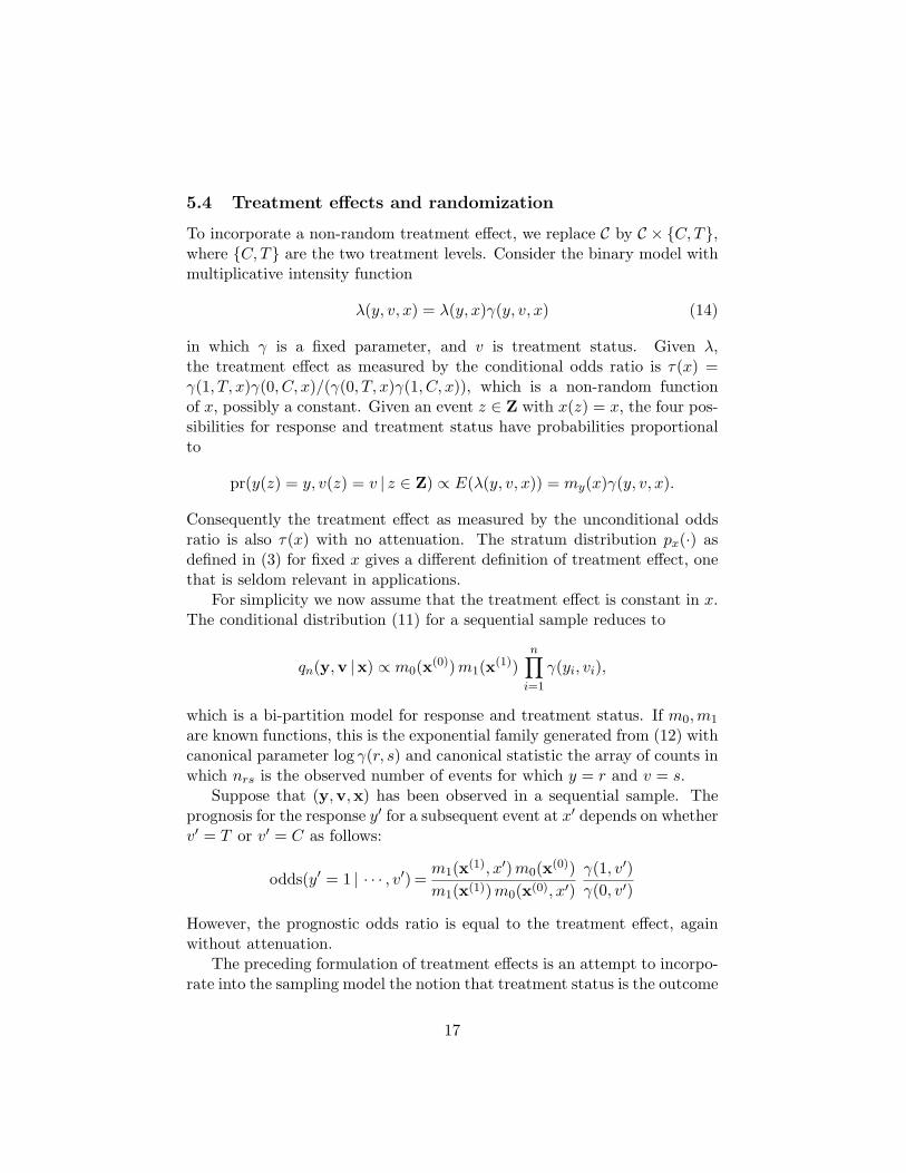
of a random process. The model with constant treatment effect can be writ-ten in multiplicative form λ(y, x)γ(y, v) as an intensity on C × {C, T} × X .The graphical representation with one node for each random element

x y

λ

v..................................................... ............. ..................................................................

........................................................................

........................................................................

....................................................................................................................... .............

shows that treatment status is conditionally independent of (λ,x) given y.Although the concept of treatment assignment is missing, the multiplicativeintensity model describes accurately what is achieved by randomization. Thepoint process of events is such that treatment status v(z) is conditionallyindependent of x(z) given the response y(z).

6 Interference

6.1 Definition

Let px(·) or p(· |x) be a set of distributions defined for arbitrary finite con-figurations x. Lack of interference is a mathematical property ensuring thatthe n-dimensional distribution px(·) is the marginal distribution of the n+1-dimensional distribution px,x′(·) after integrating out the last component. Insymbols px(A) = px,x′(A× C) for A ⊂ Cn, or

p(y ∈ A |x) = p((y, y′) ∈ A× C | (x, x′))

if applied to conditional distributions. When this condition is satisfied, thedistribution of the first n components is unaffected by the covariate value forsubsequent components. This is also the Kolmogorov consistency conditionfor a C-valued process in which the joint distribution of Y (u1), . . . , Y (un) de-pends on the covariate values x(u1), . . . , x(un) on those units. It is satisfiedby regression models such as (1), (3) and (4).

In the statistical literature on design, interference is usually understoodin the physical or biological sense, meaning carry-over effects from treatmentapplied to neighbouring plots. For details and examples, see Cox (1958) orBesag and Kempton (1986). The definition does not distinguish betweenphysical interference and sampling interference, but this paper emphasizesthe latter.

To understand how sampling interference might arise, consider the sim-plest evolving-population model in which X = {x} is a set containing a singlepoint denoted by x. Let Y1, . . . be the class labels in temporal order. Given

18

λ, the number m of events in unit time is Poisson with parameter λ., so mcould be zero. However, given m, the values Y1, . . . , Ym are exchangeablewith one- and two-dimensional distributions

p1(Y1 = r |m ≥ 1) =E((1− e−λ.)λr/λ.)

E(1− e−λ.)' E(λr)

E(λ.)

p2(Y1 = r, Y2 = s |m ≥ 2) =E((1− (1 + λ.)e−λ.)λrλs/λ2

.)E(1− (1 + λ.)e−λ.)

' E(λrλs)E(λ2.)

p2(Y1 = r |m ≥ 2) =E((1− (1 + λ.)e−λ.)λr/λ.)

E(1− (1 + λ.)e−λ.)' E(λrλ.)

E(λ2.)6= p1(Y1 = r |m ≥ 1).

In general, the probability assigned to the event Y1 = r by the bivariatedistribution p2 is not the same as the probability assigned to the same eventby the one-dimensional distribution p1. The condition m ≥ 2 in p2 impliesan additional event at x, which may change the probability distributionof Y1.

Two specific models are now considered, one exhibiting interference, theother not. In the log Gaussian model

log λ0 ∼ N(µ0, 1), log λ1 ∼ N(µ1, 1)

are independent random intensities. For a low-intensity value (µ0, µ1) =(−5,−4), we find by numerical integration that p1(Y1 = 0) = 0.272 whereasp2(Y1 = 0) = 0.201, so the interference effect is substantial. The lim-iting low-intensity approximations are 0.269 and 0.193 respectively. For(µ0, µ1) = (−1, 0) the mean intensities are (e−1/2, e1/2), and the differenceis less marked: p1(Y1 = 0) = 0.310 versus p2(Y1 = 0) = 0.291.

By contrast, consider the gamma model in which

λ0 ∼ G(α0θ, α0), λ1 ∼ G(α1θ, α1),

are independent with mean E(λr) = αrθ and variance αrθ2. The total

intensity is distributed as λ. ∼ G(α.θ, α.) independently of the ratio, whichhas the beta distribution λ0/λ. ∼ B(α0, α1). On account of independence,we find that p1(Y1 = 0) = p2(Y1 = 0) = α0/α., so interference is absent.

6.2 Over-dispersion

Suppose that events are grouped by covariate value, so that T.(x) is the ob-served number of events at x, and Tr(x) is the number of those who belong

19

to class r. Over-dispersion means that the variance of Tr(x) exceeds the bi-nomial variance, and the covariance matrix of T (x) exceeds the multinomialcovariance. However, units having distinct x-values remain independent.This effect is achieved by a Cox process driven by a completely independentrandom intensity taking independent values at distinct points in X . Sinceunits having distinct x-values remain independent, it suffices to describe theone-dimensional marginal distributions of the class totals at each point in X .

Under the gamma model, the class totals at x are independent negativebinomial random variables with means E(Tr) = γαr and variances γαr(1 +γ). Given the total number of events at x, the conditional distribution isDirichlet-multinomial

p(T = t |T. = m) =m! Γ(α.)

Γ(m + α.)

∏

r∈C

Γ(tr + αr)tr! Γ(αr)

for non-negative tr such that t. = m. The sequence of values Y1, . . . , Ym isexchangeable, and, since there is no interference, the marginal distributionsare independent of m:

pr(Y1 = r |m) = αr/α. = πr

pr(Y1 = r, Y2 = s |m) = πrπs +{

πr(1− πr)/(α. + 1) r = s−πrπs/(α. + 1) otherwise.

Because of interference, no similar results exist for the log Gaussian model.

7 Computation

7.1 Parameter estimation

Since x and y are both generated by a random process, the likelihood func-tion is determined by the joint density. However, the joint distributiondepends on the infinite-dimensional nuisance parameter ν(dx), which gov-erns primarily the marginal distribution of x. It appears that the marginaldistribution of x must contain very little information about intensity ratios,so it is natural to use the conditional distribution given x for inferentialpurposes. Likelihood calculations using the exact conditional distribution(7)–(9) or the limit distributions (11) and (12) are complicated, thoughperhaps not impossible. We focus instead on parameter estimation usingunbiased estimating equations.

Let mr(x) = E(λr(x)) be the mean intensity function for class r, m.(x) theexpected total intensity at x, ρr(x) = E(λr(x)/λ.(x)) the expected value of

20

the intensity ratio at x, and πr(x) = mr(x)/m.(x) the ratio of expectedintensities. Sampling bias is the key to the distinction between ρ(x), themarginal distribution for fixed x, and π(x), the conditional distribution forrandom x generated by a sequential sample from the process.

Consider a sequential sampling plan in which the observation consists ofthe events Zt for fixed t. The number of events #Zt, the values y(z), x(z)and π(x) = π(x(z)) for z ∈ Zt are all random. It is best to regard Zt as arandom measure in C × X whose mean has density tmy(x) ν(dx) at (y, x).The expected number of events in the interval dx is tm.(x)ν(dx), and theexpected number of events of class r in the same interval is tmr(x)ν(dx).For a function h:X → R, additive functionals have expectation

E

(∑

Zt

h(x(z)))

= t

∫

Xh(x) m.(x) ν(dx),

E

(∑

Zt

h(x(z)) yr(z))

= t

∫

Xh(x) mr(x) ν(dx),

where y(z) is the indicator function for the class, i.e. yr(z) = 1 if the classis r. It follows that the sum Tr =

∑Z h(x) (yr(z) − πr(x)) has exactly

zero mean for each function h. This first-moment calculation involves onlythe first-order product densities. If it were necessary to calculate E(T |x)given the configuration x, we should begin with the joint distribution or theconditional distribution (9). Because of interference, E(T |x) is not zero,nor is E(T |#Zt). Consequently, the moment calculations in this sectionare fundamentally different from those of McCullagh (1983) or Zeger andLiang (1986).

The covariance of Tr and Ts is a sum of three terms, one associated withintrinsic Bernoulli variability, one with spatial correlation, and one withinterference. The expressions are simplified here by setting h(x) = 1.

cov(Tr, Ts) = t

∫

X[πr(x)δrs − πr(x)πs(x)]m.(x) ν(dx)

+ t2∫

X 2[πrs(x, x′)− πr.(x, x′)πs.(x′, x)]m..(x, x′) ν(dx) ν(dx′)

+ t2∫

X 2∆r.(x, x′)∆s.(x′, x)m..(x, x′) ν(dx) ν(dx′). (15)

In these expressions, mrs(x, x′) = E(λr(x)λs(x′)) is the second-order prod-uct density, and πrs(x, x′) = mrs(x, x′)/m..(x, x′) is the bivariate distribu-tion for ordered pairs of distinct events. Roughly speaking, πr.(x, x′) is theprobability that the event at x is of class r given that another event occurs

21

at x′. The difference ∆r.(x, x′) = πr.(x, x′) − πr(x), which is a measure ofsecond-order interference, is zero for conventional models. Both the gammaand log-normal models exhibit interference, but the homogeneous gammamodel has the special property of zero second-order interference.

The first integral in (15) can be consistently estimated by summationof πr(x)δrs − πr(x)πs(x) over x. The second and third integrals can beestimated in the same way by summation over distinct ordered pairs.

The marginal mean for an event in stratum x is E(yr(x)) = ρr(x) asdetermined by the logistic-normal integral, and the difference yr(x)− ρr(x)is the basis for estimating equations associated with hierarchical regressionmodels (Zeger and Liang 1986; Zeger, Liang and Albert 1988). If in factthe x-values are generated by the process itself, the estimating function∑

Z h(x)(yr(z)−ρr(x(z))) has expectation∫X h(x)(π(x)−ρ(x))m.(x) ν(dx),

which is not zero and is of the same order as the sample size. Conventionalestimating equations are biased for the marginal mean and give inconsistentparameter estimates. Similar remarks apply to likelihood-based estimates.The correct likelihood function (9) takes account of the sampling plan andgives consistent estimates; the incorrect likelihood (3) gives inconsistent es-timates.

For the binary case k = 2, we write π(x) = π1(x) and revert to the usualnotation with y = 0 or y = 1. If we use a linear logistic parameterizationlogit(π(x)) = β′x, the parameters can be estimated consistently using ageneralized estimating equation of the form X ′W (Y − π) = 0 with a suitablechoice of weight matrix W depending on x. Recognizing that the target isπ(x) rather than ρ(x), the general outline described by Liang and Zeger(1986) can be followed, but variance calculations need to be modified toaccount for interference as in (15).

The functional yry′s − πrs(x, x′) of degree two for ordered pairs of dis-

tinct events also has zero expectation for each r, s. The additive combination∑h(x, x′)(yry

′s−πrs(x, x′)) can be used as a supplementary estimating func-

tion for variance and covariance components. However, variance calculationsare much more complicated.

7.2 Classification and prognosis

By contrast with likelihood calculations, the prognostic distribution for asubsequent event at x′ is relatively easy to compute. For the log Gaussianmodel in section 5.2, the prognostic distribution is a kernel function

log pr(Y (x′) = r | · · ·) = log mr(x′) +∑

x∈x(r)

K(x, x′) + const

22

0 1 2 3 4

0.0

0.2

0.4

0.6

0.8

1.0

x[obs]

as.

num

eric(

y[ob

s])

0 1 2 3 4

0.0

0.2

0.4

0.6

0.8

1.0

x[obs]

as.

num

eric(

y[ob

s])

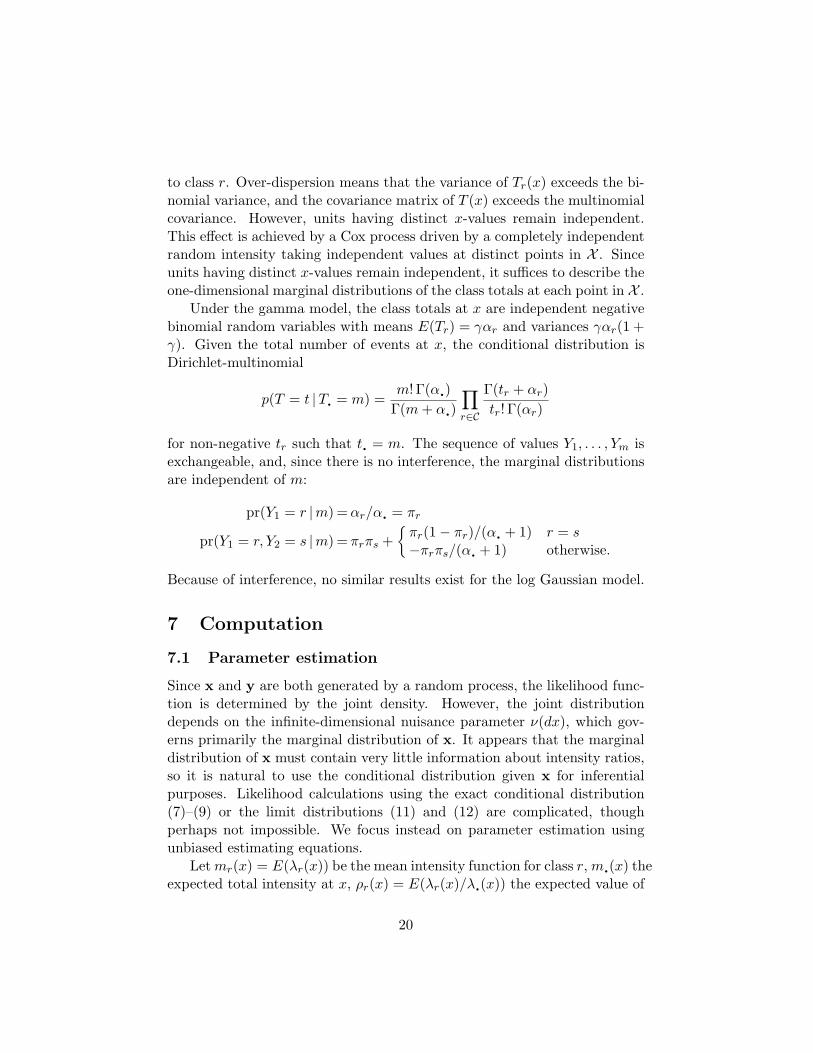
Figure 1: Prognostic probability computed for the homogeneous gammamodel with K(x, x′) = exp(−(x−x′)2) and four values of α from 0.05 to 0.5.The two sample configurations of 50 events are indicated by dots at y = 0and y = 1.

for r ∈ C. If necessary, unknown parameters can be estimated by cross-validation (Wahba, 1985). The theory in section 3 requires K to be a propercovariance function defined pointwise, but the prognostic distribution is welldefined for generalized covariance functions such as −γ|x − x′|2 for γ ≥ 0,provided that the functions log mr(x) span the kernel of the process.

The gamma model presents more of a computational challenge becausethe prognostic distribution is a ratio of permanents,

pr(Y (x′) = r | · · ·) ∝ perαr(K[x(r), x′])/perαr

(K[x(r)]),

which are notoriously difficult to compute. As it happens, the permanentratio is easier to approximate than the permanent itself. For two configu-rations of 50 events, Fig. 1 shows the prognostic probability pr(Y (x′) = 1)computed for the homogeneous gamma model with k = 2 and X = (0, 4).Permanent ratios were approximated analytically using a cycle expansiontruncated after cycles of length 4. In the homogeneous gamma model, theone-dimensional conditional probability q1(y = 1 |x) for a single event is1/2 for every x, so the prognostic probability graphs in Fig. 1 should not beconfused with regression curves.

23

8 Summary

8.1 Conventional random effects models

The statistical model (3) has an observation space {0, 1}n for each sample ofsize n, and a parameter space with four components (α, β, σ, τ). Everythingelse is incidental. The random process η used as an intermediate constructin the derivation of the distribution is not a component of the observationspace nor is it a component of the parameter space. In principle, model (3)could have been derived directly without the intermediate step (2), so directinference for η is impossible in (3). On account of the consistency condition(5), we can compute the conditional probability of any event such as

E(Y (u′) |y) = E

(eα+βx′+η(x′)

1 + eα+βx′+η(x′)

∣∣∣∣ y)

=px,x′(y, 1)

px(y), (16)

using the model distribution with an additional unit having x(u′) = x′.Sample-space inferences of this sort are accessible directly from (3), butinference for η is not. Similar remarks apply to the Gaussian model (1), inwhich case the conditional expected value (16) is a generalized smoothingspline in x′.

Since the likelihood function does not determine the observation space,we look to the likelihood function only for parameter estimation, not forinferences about the sample space or subsequent values of the process. Thisinterpretation of model and likelihood is neutral in the Bayes/non-Bayesspectrum. It is consistent with (2) as a partially Bayesian model with pa-rameters (α, β, η), in which the Gaussian process serves as the prior distri-bution for η. The Bayesian formulation enables us to compute a posteriordistribution for η(x′) whether it is of interest or not. Despite the formalequivalence of (2) as a partially Bayesian model, and (3) as a non-Bayesianmodel, the two formulations are different in a fundamental way. The treat-ment effect is ordinarily defined as the ratio of success odds for a treatedindividual to that of an untreated individual having the same baseline co-variate values. Because of parameter attenuation, the value obtained forthe partially Bayesian model (2) is not the same as that for the marginalmodel (3). Both calculations are unit-specific, so this distinction is not adifference between subject-specific and population-averaged effects. Thispaper argues that neither definition is appropriate because neither modelaccounts properly for sampling biases.

24

8.2 Subject-specific and population-average effects

For all models considered in this paper, including (1)–(4), the probabilitiesare unit specific. That is to say, each regression model specifies the responsedistribution for every unit, and the joint distribution for each finite subsetof units. Treatment effect is measured by the odds ratio, which may varyfrom unit to unit depending on the covariate value. The population averageeffect, if it is to be used at all, must be computed after the fact by averagingthe treatment effects over the distribution of x-values for the units in thetarget population. Note the distinction between unit u and subject s(u):two distinct units u, u′ in a crossover or longitudinal design correspond tothe same patient or subject if s(u) = s(u′). This block structure is assumedto be encoded in x.

Numerous authors have noted a close parallel between (2) and the one-dimensional marginal distributions associated with (3). Specifically, if ηu isa zero-mean Gaussian variable,

logit pr(Y (u) = 1 | η; x) = α + βx(u) + ηu, (17)

implieslogit pr(Y (u) = 1; x) ' α∗ + β∗x(u) (18)

by averaging over ηu for fixed u. Zeger, Liang and Albert (1988) give an ac-curate approximation for the attenuation ratio τ = β∗/β ≤ 1, which dependson the variance of ηu. Neuhaus, Kalbfleisch and Hauck (1991) confirm theaccuracy of this approximation. They also give a convincing demonstrationof the magnitude of the attenuation effect by analyzing a study of breast dis-ease in two different ways. Maximum likelihood estimates α, β were obtainedby maximizing an approximation to the integral (3) using a software pack-age egret. The alternative, generalized estimating equations using (18) forexpected values supplemented by an approximate covariance matrix, givesestimates α∗, β∗ of the attenuated parameters. The attenuation ratios β∗/βwere found to be approximately 0.35, in good agreement with the Taylorapproximation.

In biostatistical terminology, the regression parameters α, β in (17) arecalled subject-specific or cluster-specific, while the parameters in (18) arecalled population-averaged effects (Zeger et al. 1988). The terms ‘marginalparameterization’ (Glonek and McCullagh 1995), ‘marginal model’ (Hea-gerty 1999), and even ‘marginalized model’ (Schildcrout and Heagerty 2007),are also used in connection with (18). Certainly, it is important to distin-guish one from the other because the parameter values are very different.

25

Nonetheless, the population-average terminology is misleading because bothexpressions (17), (18) refer to a specific unit labelled u, and hence to a spe-cific subject s(u), not to a randomly selected unit or subject. The bivariateand multivariate version (3) is also specific to the particular set of units hav-ing covariate configuration x. In other words, both of these are conventionalregression models in which concept of random sampling of units is absent.

Apart from minor differences introduced by approximating the one-dimensional integral by (18), and similar approximations for bivariate andhigher-order distributions, these are in fact the same model. They havedifferent parameterizations, and they use different methods to estimate theparameters, but the distributions are the same. The distinction between thepopulation-average approach and the cluster-specific approach is not a dis-tinction between models, but a distinction between two parameterizationsof essentially the same model, and two methods for parameter estimation.

Having established the point that there is only one regression model, itis necessary to focus on the parameterizations and to ask which parame-terization is most natural, and for what purpose. Heagerty (1999) pointsout that individual components of β in the subject-specific parameteriza-tion are difficult to interpret unless the subject-specific effect ηu is known.Neuhaus et al. (1991, section 6) note that since each individual has herown latent risk, the model invites an unwarranted causal interpretation.Galbraith (1991) criticizes the interventionist interpretation of parametersin (17), and points out correctly that additional assumptions are requiredto justify this interpretation in an observational study. If each pair of unitshaving different treatment levels is necessarily a distinct pair of individualsor subjects, the treatment effect involves a comparison of distributions fortwo distinct subjects.

From this author’s point of view, ephemeral unit-specific, subject-specificor cluster-specific effects such as ηu or η(x(u)) are best regarded as ran-dom variables rather than parameters, a distinction that is fundamental instatistical models. Given the parameters, the conventional model specifiesthe probability distribution for each unit and each set of units by integra-tion. The intermediate step (17) shows a random variable arising in thiscalculation, leading to the joint distribution (3) whose one-dimensional dis-tributions are well approximated by (18). Two units u, u′ having the samebaseline covariate values but different treatment levels have different re-sponse distributions. The treatment effect is the difference between theseprobabilities, usually measured on the log odds ratio scale. Although es-tablished terminology suggests otherwise, the treatment component of β∗

in (18) is the treatment effect specific to this pair of units u, u′. If these

26

units represent the same subject in a controlled crossover design, an in-terventionist interpretation is appropriate. Otherwise, if two units havingdifferent treatment levels necessarily represent distinct subjects, β∗ is thedifference of response probabilities for distinct subjects, so there can be nointerventionist interpretation.

8.3 Implications for applications

Consider a market research study of consumer preferences for a set of prod-ucts such as breakfast cereals. The relevant information is extracted from adatabase in which each purchase event is recorded together with the storeinformation and consumer information. Breakfast cereal purchases are therelevant events. Following conventional notation, i denotes the purchaseevent, Yi is the brand purchased, and xi is a vector of covariates, some store-specific and some consumer-specific. The aim is to study how the marketshare pr(Yi = r |xi = x) depends on x, possibly using a multinomial responsemodel of the form (4). The random effects may be associated with store-specific variables such as geographic location, or consumer-specific variablessuch as age or ethnicity. The treatment effect may be connected with pric-ing, product placement or local advertising campaigns.

As I see it, the conventional paradigm of a stochastic process defined ona fixed set of units is indefensible in applications of this sort. Most purchaseevents are not purchases of breakfast cereals, so the relevant events (cerealpurchases) are defined by selecting from the database those that are inthe designated subset C. An arbitrary choice must be made regarding theinclusion of dual-use materials such as grits and porridge oats. Rationally,the model must be defined for general response sets, and we must then insistthat the model for the subset C′ ⊂ C be consistent with the model for C.Consistency means only that the two models are non-contradictory; theyassign the same probability to equivalent events. The evolving populationmodel with a fixed observation period is consistent under class restriction,but the conventional logistic model (4) with random effects is not.

The notation used above is conventional but ambiguous. The marketshare of brand r in stratum x is the limiting fraction of events in stra-tum x that are of class r, which is λr(x)/λ.(x) for both (4) and the evolvingpopulation model. The expected market share is the stratum probabilitypr(Yi = r | i: xi = x), which may be different from the conditional probabil-ity given xi for fixed i. However, the central concept of a fixed unit i is clearlynonsense in this context, so the standard interpretation of pr(Yi = r |xi = x)for fixed i is unsatisfactory.

27

The situation described above arises in numerous areas of applicationsuch as studies of animal behaviour, studies of crime patterns, studies ofbirth defects, and the classification of bitmap images of handwritten decimaldigits. The events are animal interactions, crimes, birth defects and bitmapimages. The response is the type of event, so C is a list of behaviours, crimetypes, birth defects or the ten decimal digits. This list is exhaustive onlyin the sense that events of other types are excluded. Hence the need forconsistency under class restriction.

In the biostatistical literature, which deals exclusively with hierarchicalmodels, an expression such as E(Yi |Xi = x) is usually described as a condi-tional expectation, but is often interpreted as the marginal mean responsefor those units i such that Xi = x. I don’t mean to be unduly critical herebecause there can be no ambiguity if these averages are equal, as they arein a hierarchical model for an exchangeable process. For an auto-generatedprocess, these averages are usually different. It is not easy to make sense ofthe literature in this broader context given that one symbol is used for twodistinct purposes. In order to make the hierarchical formulation compatiblewith the broader context of the evolving population model, it is necessaryto interpret (3) and (4) as stratum distributions, not conditional distribu-tions. Once the distinction is made, it is immediately apparent that thestratum distribution does not determine the conditional probability given xfor a sequential sample. Consequently, probability calculations using thestratum distribution, and efforts to estimate the parameters by using thewrong likelihood function (3) must be abandoned.

8.4 Sampling bias

The main thrust of this paper is that, when the units are unlabelled andsampling effects are properly taken into account using the evolving popu-lation model as described in sections 3, 5.4, and 7.1, there is no parameterattenuation. If the intensities are such that λ1(x) has the same mean aseα+βxλ0(x), the correct version of (17) and (18) for an auto-generated unitu ∈ Zt is

logit pr(Y (u) = 1 |λ, u ∈ Zt) = log λ1(x(u))− log λ0(x(u))= α + βx(u) + η(x(u)),

logit pr(Y (u) = 1 |u ∈ Zt) = log m1(x(u))− log m0(x(u))= α + βx(u),

28

with no approximation and no attenuation. The distinction described insection (8.2) between two parameterizations is simply incorrect for auto-generated units.

The subject-specific approach takes aim at the right target parameterin (17), but the conventional likelihood or hierarchical Bayesian calculationleads to inconsistency when sampling bias is ignored in the steps leadingto (3). Sample x-values occur preferentially at points where the total in-tensity λ.(·) is high, which is not the case for a predetermined x. As a re-sult, parameter estimates from (6) are inflated by the factor 1/τ where τ isthe apparent attenuation factor. The inflation factor reported by Neuhauset al. (1991) is a little less than 3, so the bias in parameter estimates is farfrom negligible. The population-average procedure commits the same errortwice, by first defining the stratum probability ρ(x) as the target, and thenfailing to recognize that E(Y |x) 6= ρ(x) for a random sample. But a fortu-itous ambiguity of the conventional notation E(Y |x) allows it to estimatethe right parameter π(x) consistently by estimating the wrong parameterρ(x) inconsistently.

For a sequential sample, the parameters α, β in (17) are exactly equalto the parameters α∗, β∗ in the marginal distribution (18). The apparentattenuation arises not because of a real distinction between subject-specificand population-averaged effects, but because of failure to recognize andmake allowance for sampling effects in the statistical model.

9 Acknowledgement

I am grateful to the referees for helpful comments on an earlier version, andto J. Yang for the R code used to produce Figure 1.

References

[1] Baddley, A. and Jensen, E.B (2005) Stereology for Statisticians. BocaRaton, Chapman and Hall.

[2] Besag, J. (1974) Spatial interaction and the statistical analysis of latticesystems (with discussion). J. Roy. Statist. Soc. B 36, 192-236.

[3] Besag, J. and Kempton, R. (1986) Statistical analysis of field experi-ments using neighbouring plots. Biometrics 42, 231-251.

29

[4] Breslow, N.E. and Clayton, D.G. (1993) Approximate inference in gen-eralized linear mixed models. J. Amer. Statist. Assoc., 88, 9-25.

[5] Cox, D.R. (1958) Planning of Experiments Wiley, New York.

[6] Cox, D.R. (1972) Regression models and life tables. J. Roy. Statist.Soc. B 34, 187-220.

[7] Cox, D.R. and Snell, E.J. (1979) On sampling and the estimation ofrare errors. biometrika 66, 125-132.

[8] Galbraith, J.I. (1991) The interpretation of a regression coefficient. Bio-metrics 47, 1593-1596.

[9] Glonek, G.F.V. and McCullagh, P. (1995) Multivariate logistic models.J. Roy. Statist. Soc. B 57, 533-546.

[10] Green, P. and Silverman, B. (1994) Nonparametric regression and gen-eralized linear models. Chapman and Hall, London.

[11] Heagerty, P.J. (1999) Marginally specified logistic-normal models forlongitudinal binary data. Biometrics 55, 688-698.

[12] Laird, N. and Ware, J. (1982) Random effects models for longitudinaldata. Biometrics 38, 963-974.

[13] Lee, Y. and Nelder, J.A. (1996) Hierarchical generalised linear models(with discussion). J. Roy. Statist. Soc. B, 58, 619-656.

[14] Lee, Y., Nelder, J.A. and Pawitan, Y. (2006) Generalized Linear Modelswith Random Effects. London, Chapman and Hall.

[15] Liang, K-Y. and Zeger, S.L. (1986) Longitudinal data analysis usinggeneralised linear models. Biometrika 73, 13-22.

[16] McCullagh, P. (1983) Quasi-likelihood functions. Annals of Statistics11, 59-67.

[17] McCullagh, P. (2005) Exchangeability and regression models. In Cele-brating Statistics, A.C. Davison, Y. Dodge and N. Wermuth, editors.89-113.

[18] McCullagh, P. and Nelder, J.A. (1989) Generalized Linear Models.Chapman and Hall, London.

30

[19] McCullagh, P. and Yang, J. (2006) Stochastic classification models.Proc. International Congress of Mathematicians, 2006, vol. III, 669-686.

[20] McCullagh, P. and Møller, J. (2006) The permanental process. Adv.Appl. Prob. 38, 873-888.

[21] McCulloch, C.E. (1994) Maximum likelihood variance components es-timation in binary data. J. Amer. Statist. Assoc., 89, 330-335.

[22] McCulloch, C.E. (1997) Maximum-likelihood algorithms for generalizedlinear mixed models. J. Amer. Statist. Assoc., 92, 162-170.

[23] Møller, J., Syversveen, A.R. and Waagpetersen, R.P. (1998) Log Gaus-sian Cox processes. Scandinavian Journal of Statistics 25, 451-482.

[24] Neuhaus, J.M., Kalbfleisch, J.D. and Hauck, W.W. (1991) A compari-son of cluster-specific and population-averaged approaches for analyzingcorrelated binary data. Int. Statist. Rev. 59, 25-35.

[25] Schall, R. (1991) Estimation in generalized linear models with randomeffects. Biometrika, 78, 719-727.

[26] Schildcrout, J.S. and Heagerty, P.J. (2007) Marginalized models formoderate to long series of longitudinal binary response data. Biometrics63, 322-331.

[27] Shirai, T. and Takahashi, Y. (2003) Random point fields associated withcertain Fredholm determinants I: Fermion, Poisson and boson pointprocesses. J. Functional Analysis 205, 414-463.

[28] Wahba, G. (1985) A comparison of GCV and GML for choosing thesmoothing parameter in the generalized spline smoothing problem. An-nals of Statistics 13, 1378-1402.

[29] Wolfinger, R.W. (1993) Laplace’s approximation for nonlinear mixedmodels. Biometrika, 80, 791-795.

[30] Zeger, S.L. and Liang, K.-Y. (1986) Longitudinal data analysis for dis-crete and continuous outcomes. Biometrics, 42, 121-130.

[31] Zeger, S.L., Liang, K.-Y. and Albert, J.A. (1988) Models for longitudi-nal data: a generalized estimating equations approach. Biometrics 44,1049-1060.

31