Sampling and the Sampling Distribution(7) (1)
31
Sampling and the Sampling Distribution Sampling Statistics and Parameters Reasons for Sampling Taking a sample instead of conducting a census offers several advantages. 1. The sample can save money. 2. The sample can save time. 3. For given resources, the sample can broaden the scope of the study. 4. Because the research process is some times destructive, the sample can save product.
-
Upload
md-sabeel-ansari -
Category
Documents
-
view
226 -
download
3
description
sampling distribution
Transcript of Sampling and the Sampling Distribution(7) (1)
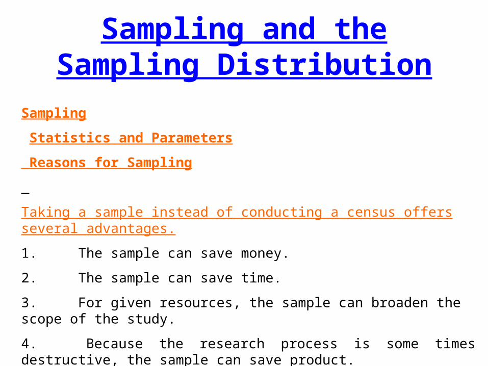
Sampling and the Sampling Distribution
Sampling
Statistics and Parameters
Reasons for Sampling
Taking a sample instead of conducting a census offers several advantages.
1. The sample can save money.
2. The sample can save time.
3. For given resources, the sample can broaden the scope of the study.
4. Because the research process is some times destructive, the sample can save product.
5. If accessing the population is impossible, the sample is the only option.
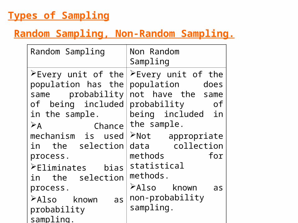
Types of Sampling
Random Sampling, Non-Random Sampling.
Random Sampling Non Random Sampling
Every unit of the population has the same probability of being included in the sample.A Chance mechanism is used in the selection process.Eliminates bias in the selection process.Also known as probability sampling.
Every unit of the population does not have the same probability of being included in the sample.Not appropriate data collection methods for statistical methods.Also known as non-probability sampling.
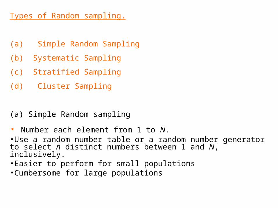
Types of Random sampling.
(a) Simple Random Sampling
(b) Systematic Sampling
(c) Stratified Sampling
(d) Cluster Sampling
(a) Simple Random sampling
• Number each element from 1 to N.•Use a random number table or a random number generator to select n distinct numbers between 1 and N, inclusively.•Easier to perform for small populations•Cumbersome for large populations
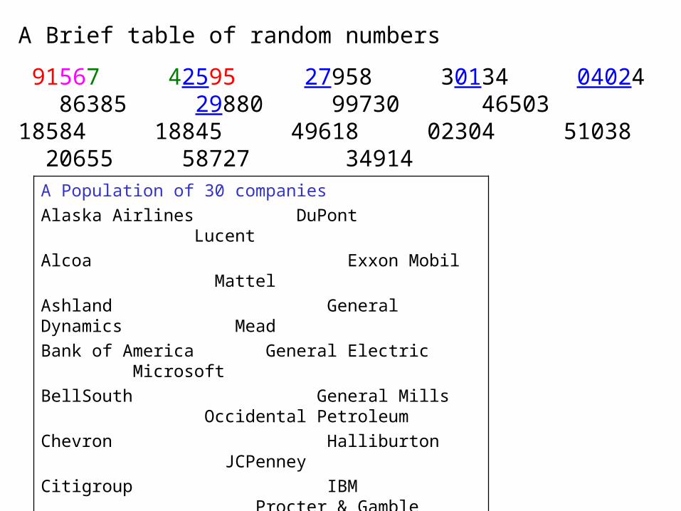
A Brief table of random numbers
91567 42595 27958 30134 04024 86385 29880 99730 46503 18584 18845 49618 02304 51038 20655 58727 34914
A Population of 30 companies
Alaska Airlines DuPont Lucent
Alcoa Exxon Mobil Mattel
Ashland General Dynamics Mead
Bank of America General Electric Microsoft
BellSouth General Mills Occidental Petroleum
Chevron Halliburton JCPenney
Citigroup IBM Procter & Gamble
Clorox Kellogg Ryder
Delta Airlines Kmart Sears
Disney Lowe’s Time Warner
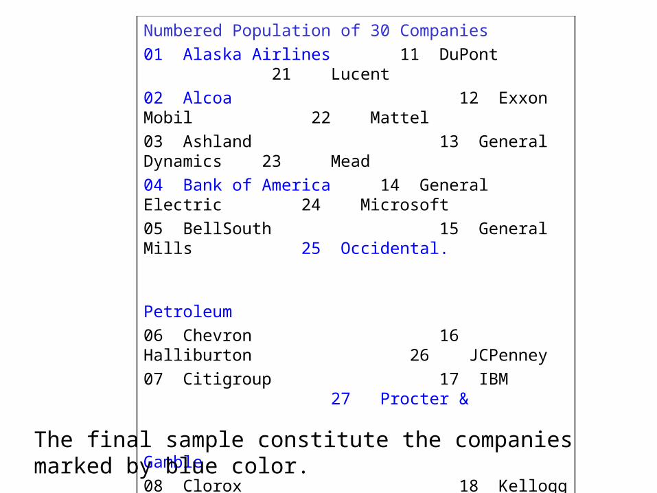
Numbered Population of 30 Companies
01 Alaska Airlines 11 DuPont 21 Lucent
02 Alcoa 12 Exxon Mobil 22 Mattel
03 Ashland 13 General Dynamics 23 Mead
04 Bank of America 14 General Electric 24 Microsoft
05 BellSouth 15 General Mills 25 Occidental.
Petroleum
06 Chevron 16 Halliburton 26 JCPenney
07 Citigroup 17 IBM 27 Procter &
Gamble
08 Clorox 18 Kellogg 28 Ryder
09 Delta Airlines 19 Kmart 29 Sears
10 Disney 20 Lowe’s 30 Time Warner
The final sample constitute the companies marked by blue color.
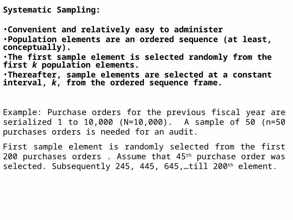
Systematic Sampling:
•Convenient and relatively easy to administer•Population elements are an ordered sequence (at least, conceptually).•The first sample element is selected randomly from the first k population elements.•Thereafter, sample elements are selected at a constant interval, k, from the ordered sequence frame.
Example: Purchase orders for the previous fiscal year are serialized 1 to 10,000 (N=10,000). A sample of 50 (n=50 purchases orders is needed for an audit.
First sample element is randomly selected from the first 200 purchases orders . Assume that 45th purchase order was selected. Subsequently 245, 445, 645,…till 200th element.
Stratified Sampling
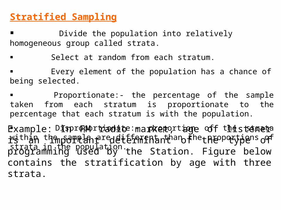
Divide the population into relatively homogeneous group called strata.
Select at random from each stratum.
Every element of the population has a chance of being selected.
Proportionate:- the percentage of the sample taken from each stratum is proportionate to the percentage that each stratum is with the population.
Disproportionate:- proportion of the strata within the sample are different than the proportions of strata in the population.
Example: In FM radio market, age of listener is an important determinant of the type of programming used by the Station. Figure below contains the stratification by age with three strata.
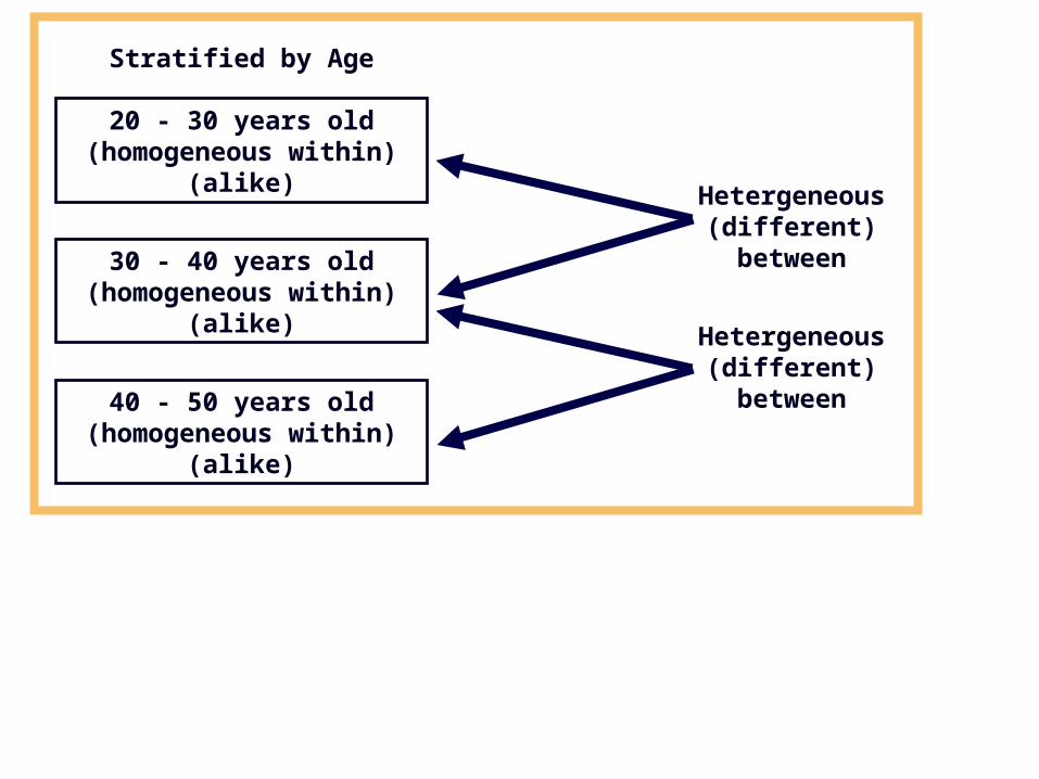
20 - 30 years old(homogeneous within)
(alike)
30 - 40 years old(homogeneous within)
(alike)
40 - 50 years old(homogeneous within)
(alike)
Hetergeneous(different)between
Hetergeneous(different)between
Stratified by Age
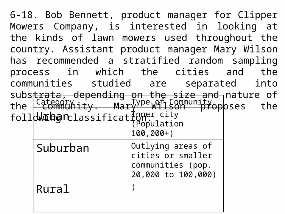
6-18. Bob Bennett, product manager for Clipper Mowers Company, is interested in looking at the kinds of lawn mowers used throughout the country. Assistant product manager Mary Wilson has recommended a stratified random sampling process in which the cities and the communities studied are separated into substrata, depending on the size and nature of the community. Mary Wilson proposes the following classification:
Category Type of Community
Urban Inner city (Population 100,000+)
Suburban Outlying areas of cities or smaller communities (pop. 20,000 to 100,000)
Rural )
Cluster Sampling
In cluster sampling, we divide the population into groups or clusters and then select a random sample of these clusters. We assume that these individual clusters are the representative of the population as a whole.
Example: If market research team is attempting to determine by sampling the average number of television per household in a large city, they could use a city map to divide the territory into blocks and then choose a certain number of blocks for interviewing. Every households in each of these blocks would be interviewed.
Advantages•More convenient for geographically dispersed populations•Reduced travel costs to contact sample elements•Simplified administration of the survey
Disadvantages•Statistically less efficient when the cluster elements are similar
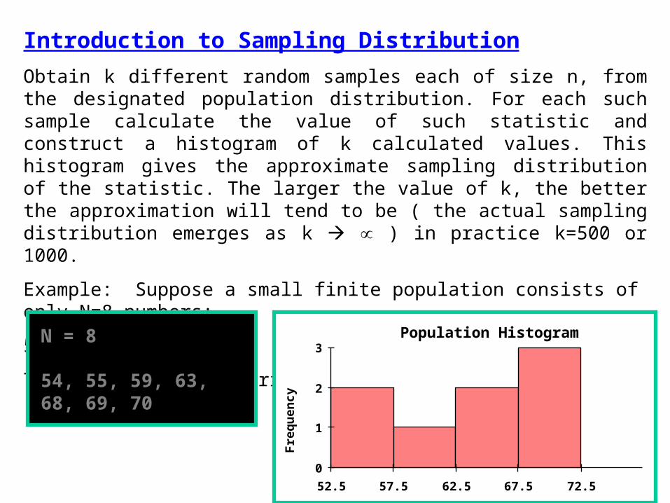
Introduction to Sampling Distribution
Obtain k different random samples each of size n, from the designated population distribution. For each such sample calculate the value of such statistic and construct a histogram of k calculated values. This histogram gives the approximate sampling distribution of the statistic. The larger the value of k, the better the approximation will tend to be ( the actual sampling distribution emerges as k ) in practice k=500 or 1000.
Example: Suppose a small finite population consists of only N=8 numbers:
54 55 59 63 64 68 69 70
The shape of the distribution of this population data.
Population Histogram
0
1
2
3
52.5 57.5 62.5 67.5 72.5
Fre
qu
ency
N = 8
54, 55, 59, 63, 68, 69, 70
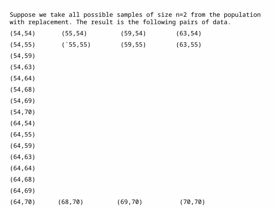
Suppose we take all possible samples of size n=2 from the population with replacement. The result is the following pairs of data.
(54,54) (55,54) (59,54) (63,54)
(54,55) (`55,55) (59,55) (63,55)
(54,59)
(54,63)
(54,64)
(54,68)
(54,69)
(54,70)
(64,54)
(64,55)
(64,59)
(64,63)
(64,64)
(64,68)
(64,69)
(64,70) (68,70) (69,70) (70,70)
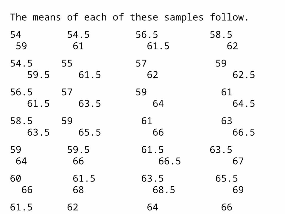
The means of each of these samples follow.
54 54.5 56.5 58.5 59 61 61.5 62
54.5 55 57 59 59.5 61.5 62 62.5
56.5 57 59 61 61.5 63.5 64 64.5
58.5 59 61 63 63.5 65.5 66 66.5
59 59.5 61.5 63.5 64 66 66.5 67
60 61.5 63.5 65.5 66 68 68.5 69
61.5 62 64 66 66.5 68.5 69 69.5
62 62.5 64.5 66.5 67 69 69.5 70
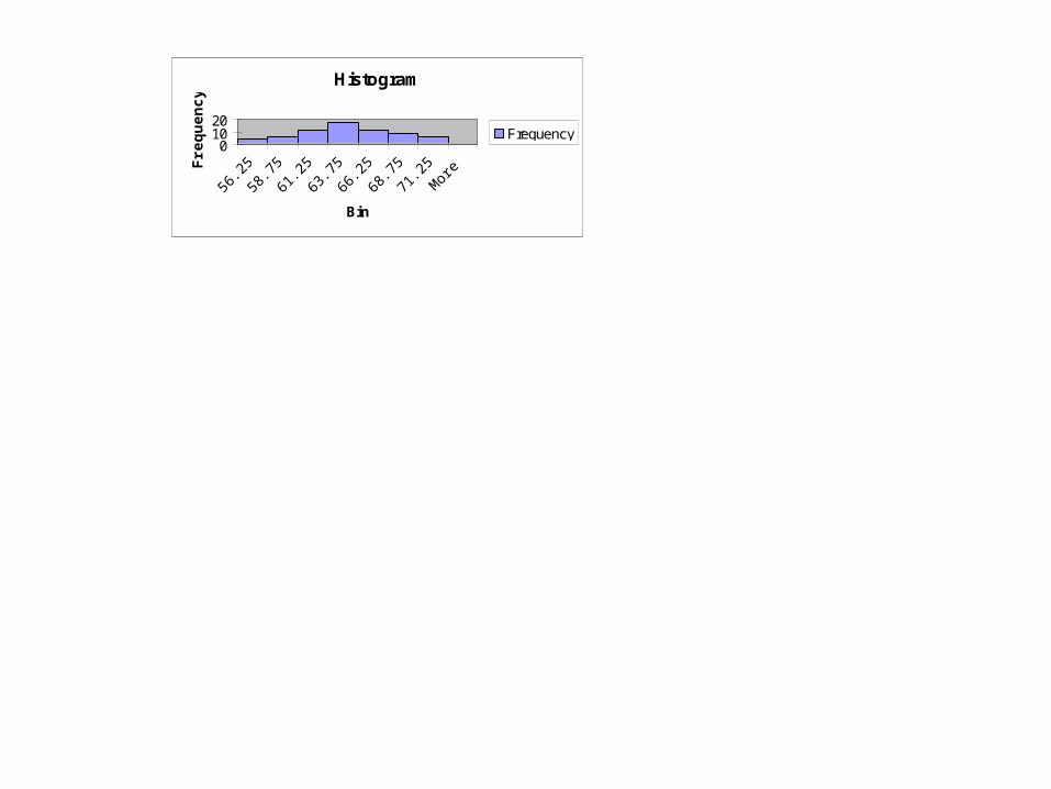
Histogram
01020
56.2558.7561.2563.7566.2568.7571.25More
BinF
req
uen
cy
Frequency
0
50
100
150
200
250
300
350
400
450
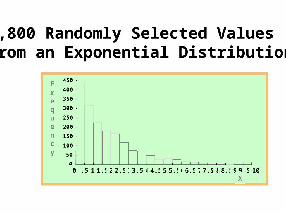
0 .5 1 1.5 2 2.5 3 3.5 4 4.5 5 5.5 6 6.5 7 7.5 8 8.5 9 9.5 10X
Frequency
1,800 Randomly Selected Values from an Exponential Distribution
Frequency
0
1
2
3
4
5
6
7
8
9
0.00 0.25 0.50 0.75 1.00 1.25 1.50 1.75 2.00 2.25 2.50 2.75 3.00 3.25 3.50 3.75 4.00
x
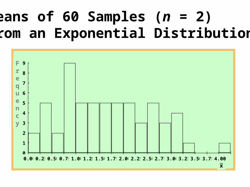
Means of 60 Samples (n = 2) from an Exponential Distribution
Frequency
x
0
1
2
3
4
5
6
7
8
9
10
0.00 0.25 0.50 0.75 1.00 1.25 1.50 1.75 2.00 2.25 2.50 2.75 3.00 3.25 3.50 3.75 4.00
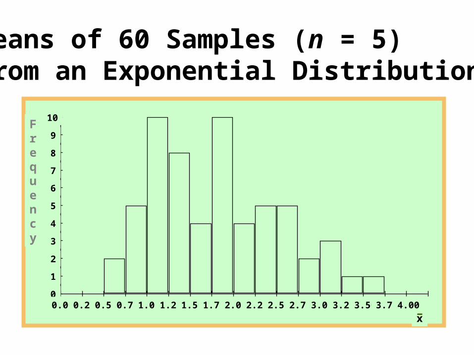
Means of 60 Samples (n = 5) from an Exponential Distribution
0
2
4
6
8
10
12
14
16
0.00 0.25 0.50 0.75 1.00 1.25 1.50 1.75 2.00 2.25 2.50 2.75 3.00
Frequency
x
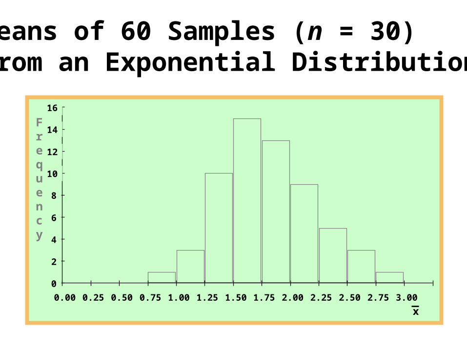
Means of 60 Samples (n = 30) from an Exponential Distribution
X
Frequency
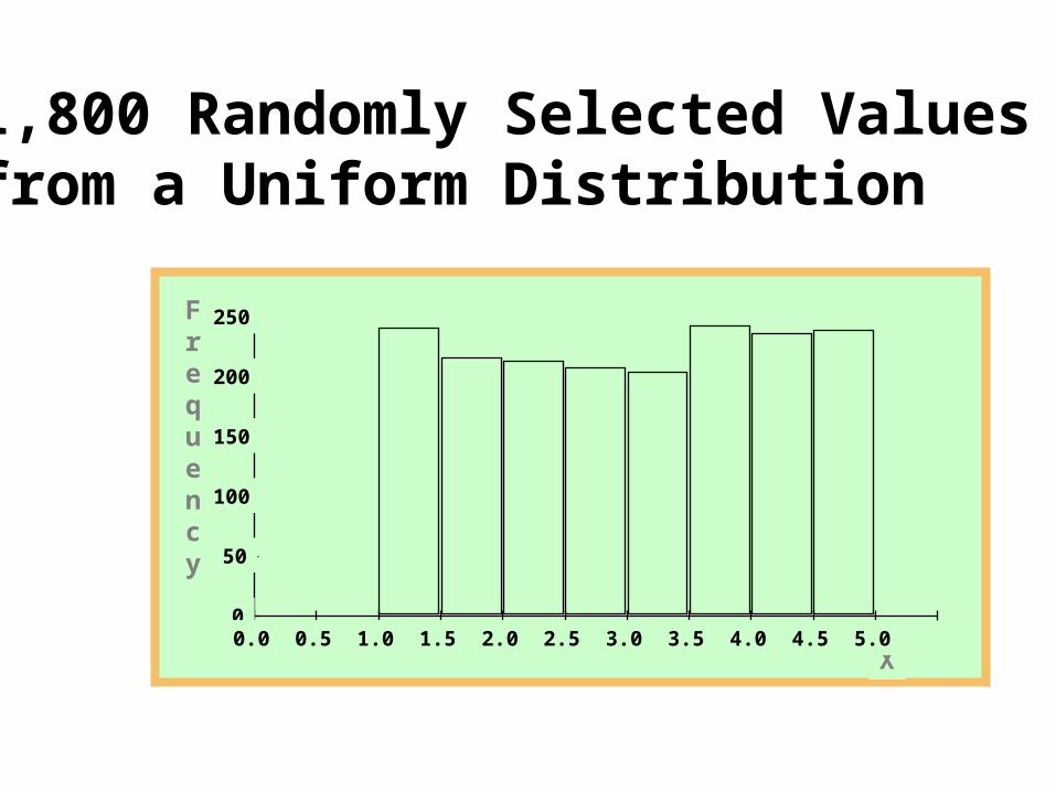
0
50
100
150
200
250
0.0 0.5 1.0 1.5 2.0 2.5 3.0 3.5 4.0 4.5 5.0
1,800 Randomly Selected Values from a Uniform Distribution
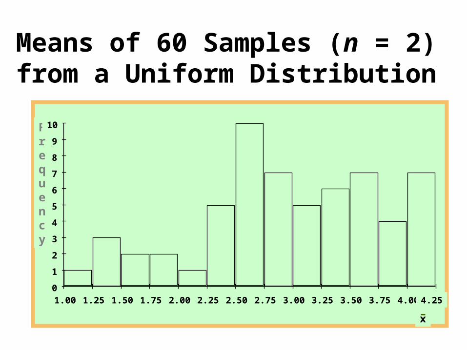
Frequency
x
0
1
2
3
4
5
6
7
8
9
10
1.00 1.25 1.50 1.75 2.00 2.25 2.50 2.75 3.00 3.25 3.50 3.75 4.00 4.25
Means of 60 Samples (n = 2) from a Uniform Distribution
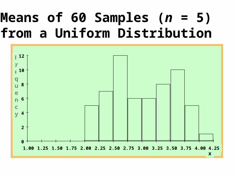
Frequency
x
0
2
4
6
8
10
12
1.00 1.25 1.50 1.75 2.00 2.25 2.50 2.75 3.00 3.25 3.50 3.75 4.00 4.25
Means of 60 Samples (n = 5) from a Uniform Distribution
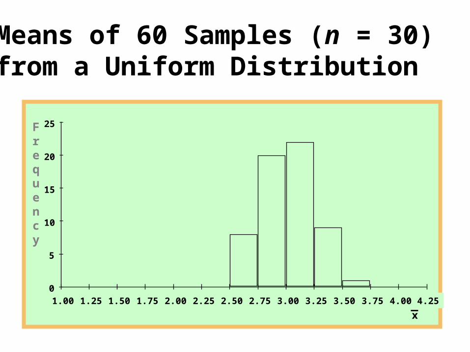
Frequency
x
0
5
10
15
20
25
1.00 1.25 1.50 1.75 2.00 2.25 2.50 2.75 3.00 3.25 3.50 3.75 4.00 4.25
Means of 60 Samples (n = 30) from a Uniform Distribution
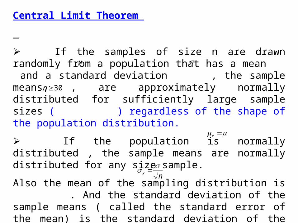
Central Limit Theorem
If the samples of size n are drawn randomly from a population that has a mean and a standard deviation , the sample means, , are approximately normally distributed for sufficiently large sample sizes ( ) regardless of the shape of the population distribution.
If the population is normally distributed , the sample means are normally distributed for any size sample.
Also the mean of the sampling distribution is . And the standard deviation of the sample means ( called the standard error of the mean) is the standard deviation of the population divided by the square root of the sample size
30n
x
nx
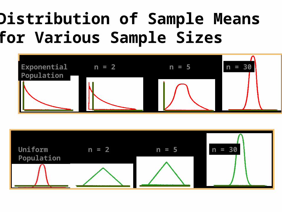
ExponentialPopulation
n = 2 n = 5 n = 30
UniformPopulation
n = 2 n = 5 n = 30
Distribution of Sample Means for Various Sample Sizes
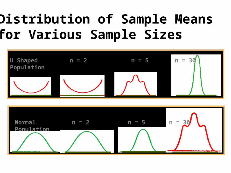
U ShapedPopulation
n = 2 n = 5 n = 30
NormalPopulation
n = 2 n = 5 n = 30
Distribution of Sample Means for Various Sample Sizes
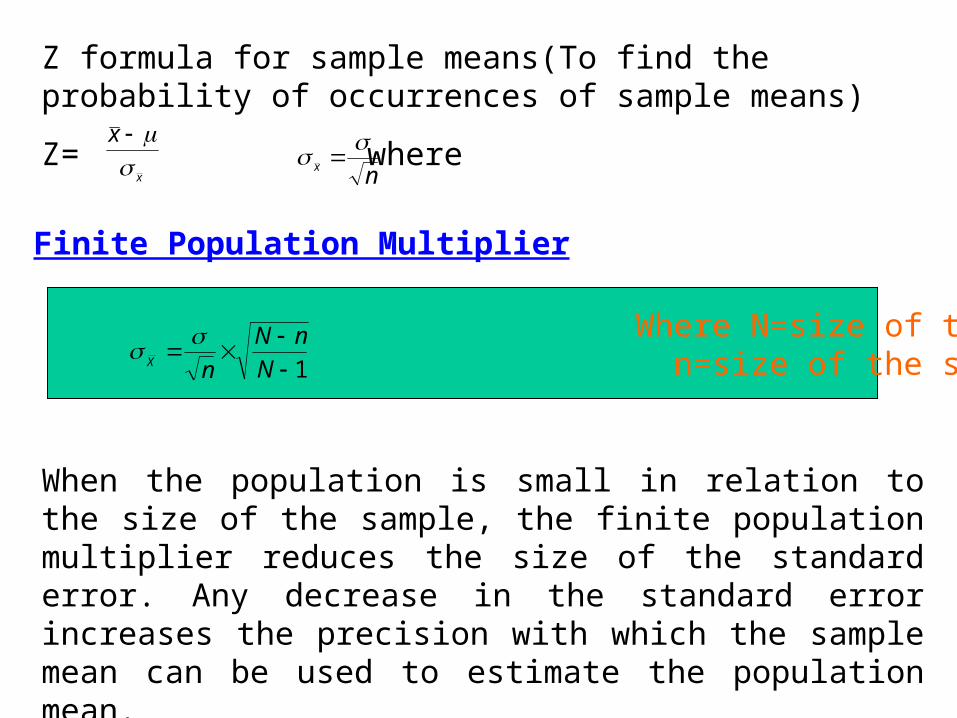
Z formula for sample means(To find the probability of occurrences of sample means)
Z= where x
x
nx
Finite Population Multiplier
Where N=size of the population n=size of the sample1
N
nN
nX
When the population is small in relation to the size of the sample, the finite population multiplier reduces the size of the standard error. Any decrease in the standard error increases the precision with which the sample mean can be used to estimate the population mean.
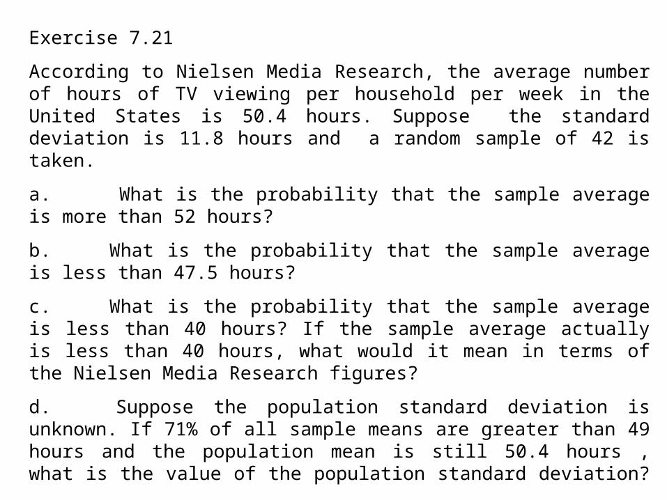
Exercise 7.21
According to Nielsen Media Research, the average number of hours of TV viewing per household per week in the United States is 50.4 hours. Suppose the standard deviation is 11.8 hours and a random sample of 42 is taken.
a. What is the probability that the sample average is more than 52 hours?
b. What is the probability that the sample average is less than 47.5 hours?
c. What is the probability that the sample average is less than 40 hours? If the sample average actually is less than 40 hours, what would it mean in terms of the Nielsen Media Research figures?
d. Suppose the population standard deviation is unknown. If 71% of all sample means are greater than 49 hours and the population mean is still 50.4 hours , what is the value of the population standard deviation?
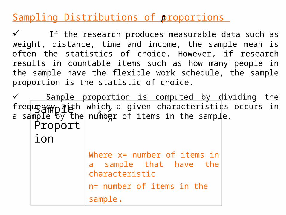
Sampling Distributions of proportions
If the research produces measurable data such as weight, distance, time and income, the sample mean is often the statistics of choice. However, if research results in countable items such as how many people in the sample have the flexible work schedule, the sample proportion is the statistic of choice.
Sample proportion is computed by dividing the frequency with which a given characteristics occurs in a sample by the number of items in the sample.
p̂
Sample
Proportion
Where x= number of items in a sample that have the characteristic
n= number of items in the sample.
n
xp ˆ
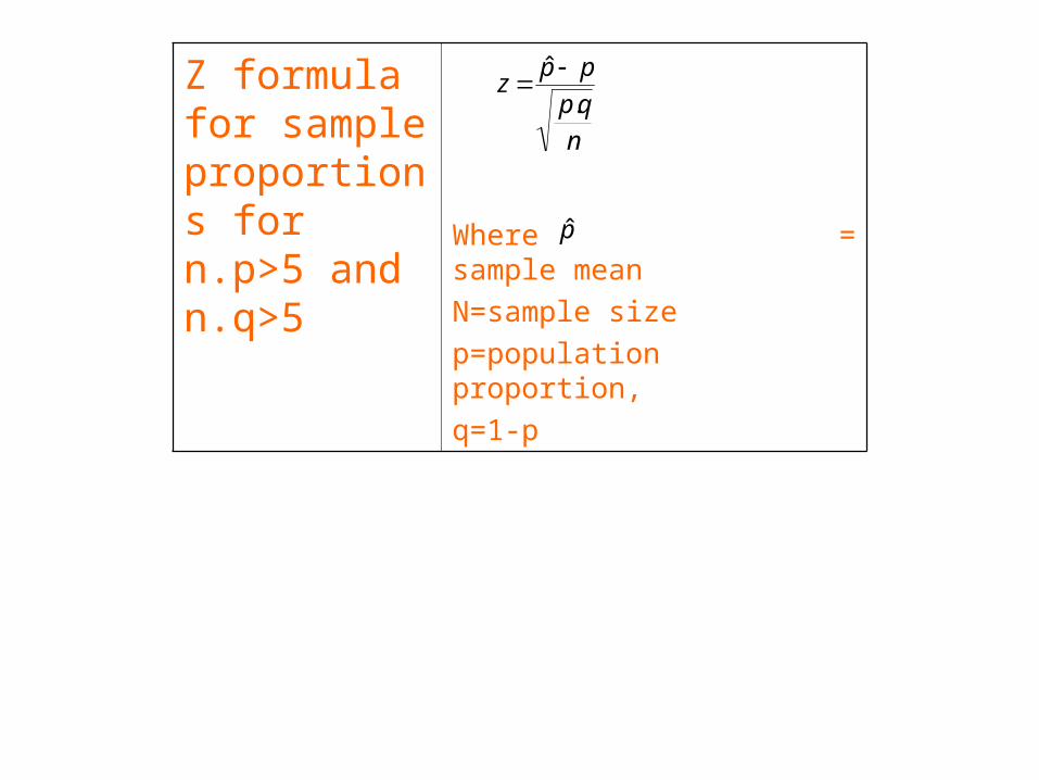
Z formula for sample proportions for n.p>5 and n.q>5
Where = sample mean
N=sample size
p=population proportion,
q=1-p
n
qp
ppz
.
ˆ
p̂
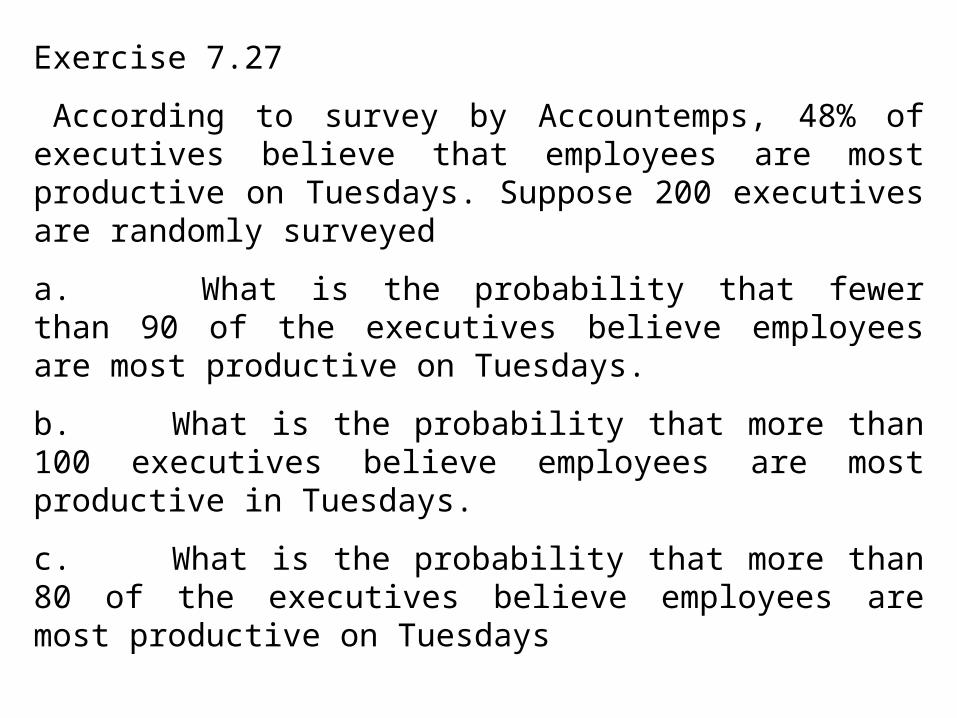
Exercise 7.27
According to survey by Accountemps, 48% of executives believe that employees are most productive on Tuesdays. Suppose 200 executives are randomly surveyed
a. What is the probability that fewer than 90 of the executives believe employees are most productive on Tuesdays.
b. What is the probability that more than 100 executives believe employees are most productive in Tuesdays.
c. What is the probability that more than 80 of the executives believe employees are most productive on Tuesdays
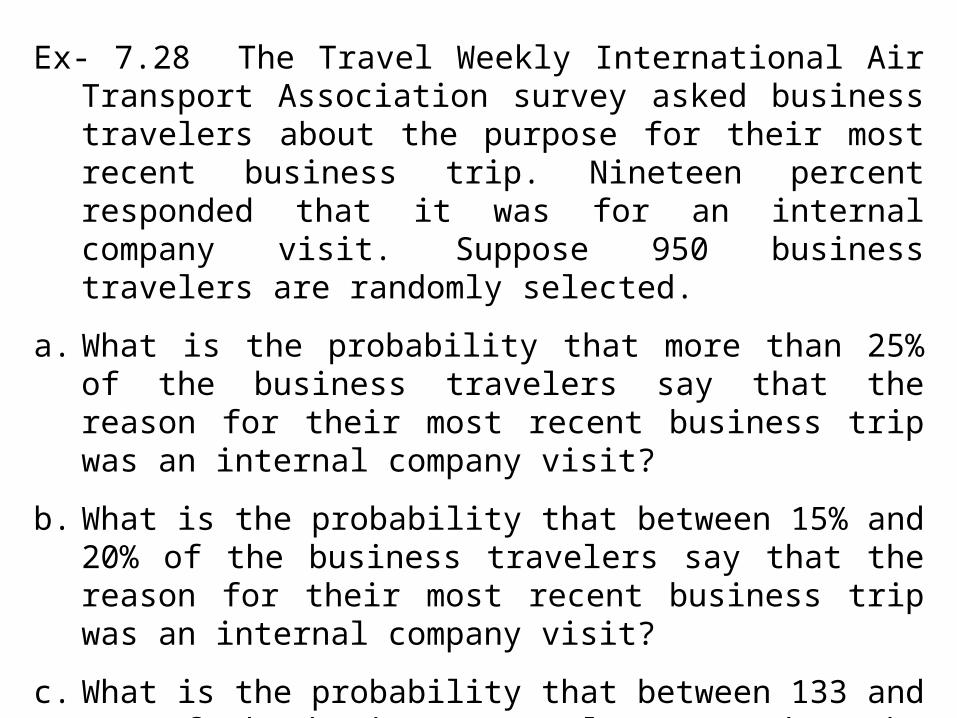
Ex- 7.28 The Travel Weekly International Air Transport Association survey asked business travelers about the purpose for their most recent business trip. Nineteen percent responded that it was for an internal company visit. Suppose 950 business travelers are randomly selected.
a. What is the probability that more than 25% of the business travelers say that the reason for their most recent business trip was an internal company visit?
b. What is the probability that between 15% and 20% of the business travelers say that the reason for their most recent business trip was an internal company visit?
c. What is the probability that between 133 and 171 of the business travelers say that the reason for their most recent business trip was an internal company visit?


![Sampling Distribution[1]](https://static.fdocuments.in/doc/165x107/577cd90d1a28ab9e78a29176/sampling-distribution1.jpg)