Sample Approximation Methods for Stochastic Program Jerry Shen Zeliha Akca March 3, 2005.
24
Sample Approximation Methods for Stochastic Program Jerry Shen Zeliha Akca March 3, 2005
-
Upload
felix-wensley -
Category
Documents
-
view
228 -
download
1
Transcript of Sample Approximation Methods for Stochastic Program Jerry Shen Zeliha Akca March 3, 2005.
Sample Approximation Methods for Stochastic Program
Jerry Shen
Zeliha Akca
March 3, 2005

Two-Stage SP with Recourse
0,..)('min xbAxTSxQxcx
)(xQWhere : Expected recourse cost of choosing x in first stage
0,)()(..'min),( yxThWyTSyqxQy
def
)(),( dPxQ

Interior sampling methods
LShaped Method (Dantzig and Infanger)
Stochastic Decomposition (Higle and Sen)
Stochastic Quasi-gradient methods (Ermoliev)

Exterior sampling methods
Monte Carlo
Quasi-Monte Carlo

Monte Carlo Sampling
Sample independently from U[0,1]d
Error estimation is comparatively easy Monte Carlo errors are of O(n-1/2) Error does depend on dimension d Can be combined with variance reduction
techniques
)(),( dPxQ
N
j
jN xQ
11 ),(

Variance Reduction Techniques
Decrease the sample variance:
-Improve statistical efficiency
-Improve time efficiency
-Decrease necessary number of random number generation
Variance Reduction Techniques
Antithetic Variables Stratified Sampling Conditional Sampling Latin Hypercube Sampling Common Random numbers Combination of these

Antithetic variables:
X1, X2 be r.v. and estimator is (X1+X2)/2
Need negatively correlation X1=h(U1,U2,..Um) X2=h(1-U1,1-U2,..1-
Um)
)]2,1(2)2()1([4
1)
2
21( XXCovXVarXVar
XXVar
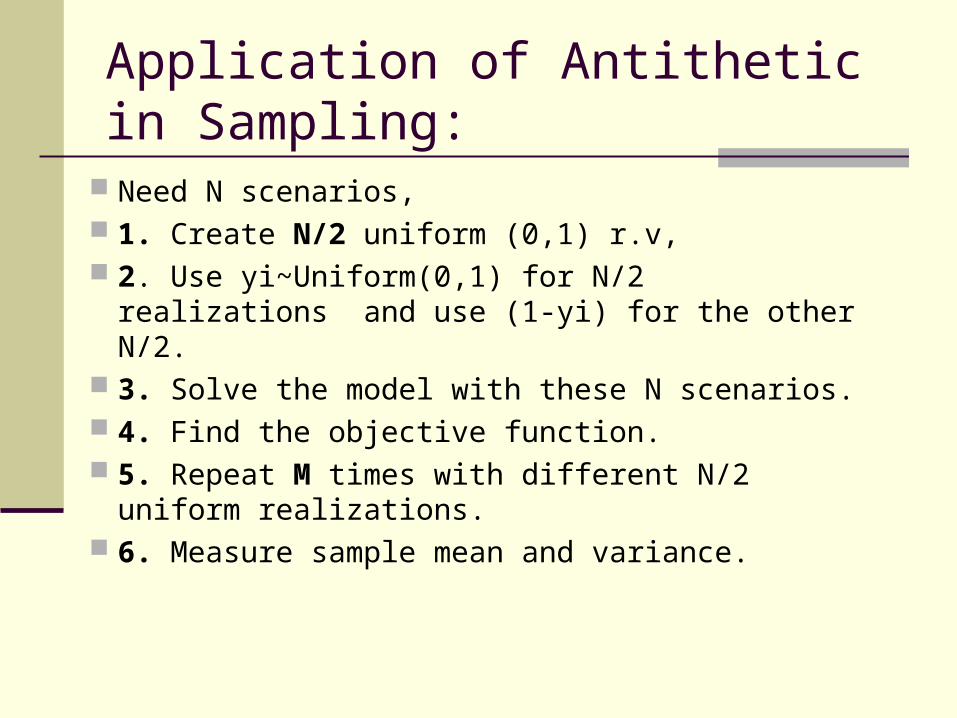
Application of Antithetic in Sampling:
Need N scenarios, 1. Create N/2 uniform (0,1) r.v, 2. Use yi~Uniform(0,1) for N/2 realizations
and use (1-yi) for the other N/2. 3. Solve the model with these N scenarios. 4. Find the objective function. 5. Repeat M times with different N/2 uniform
realizations. 6. Measure sample mean and variance.
Conditional Sampling
Use E[X|Y] to estimate X. E[X|Y]=E[X], Var(X)=E[Var(X|Y)]+Var(E[X|Y])>=Var(E[X|Y])
Stratified Sampling
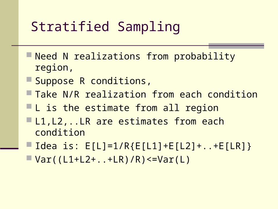
Need N realizations from probability region, Suppose R conditions, Take N/R realization from each condition L is the estimate from all region L1,L2,..LR are estimates from each condition Idea is: E[L]=1/R{E[L1]+E[L2]+..+E[LR]} Var((L1+L2+..+LR)/R)<=Var(L)
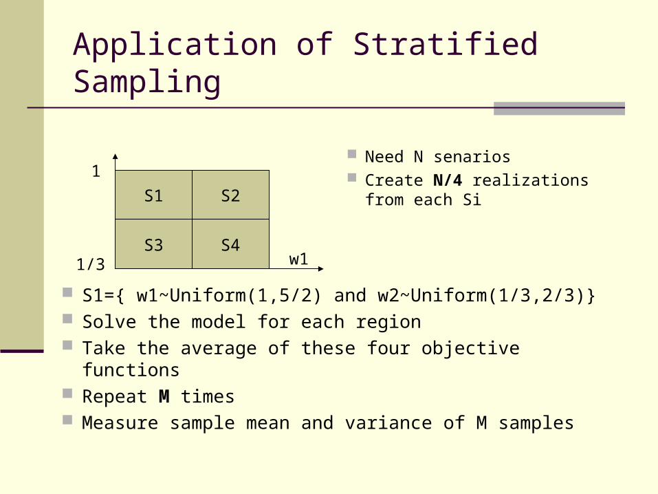
Application of Stratified Sampling
S1={ w1~Uniform(1,5/2) and w2~Uniform(1/3,2/3)} Solve the model for each region Take the average of these four objective functions Repeat M times Measure sample mean and variance of M samples
1/3
S1
S3 S4
S2
1
w1
Need N senarios Create N/4 realizations from each
Si
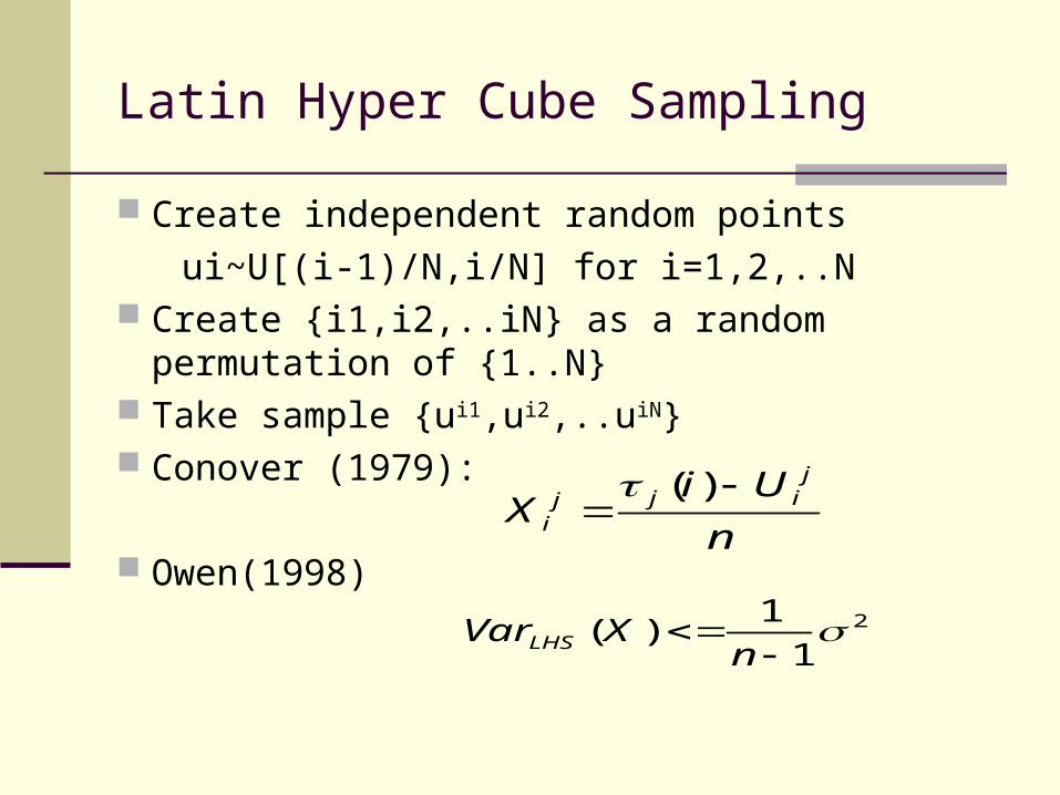
Latin Hyper Cube Sampling
Create independent random points
ui~U[(i-1)/N,i/N] for i=1,2,..N Create {i1,i2,..iN} as a random permutation
of {1..N} Take sample {ui1,ui2,..uiN} Conover (1979):
Owen(1998)
n
UiX
jijj
i
)(
2
1
1)(
n
XVarLHS

Application of LHS:
Divide the range of each input to N partition Take a realization from each partition with prob. 1/N
W1:a1 aNa3a2 ….
W2: b2b1 b3 bN….
Scenario1=(a4,b56)
Scenario2=(a6,bN)
ScenarioN=(a40,b8)
Scenariok=(a26,b3)
Random match
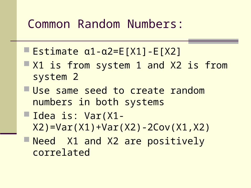
Common Random Numbers:
Estimate α1-α2=E[X1]-E[X2] X1 is from system 1 and X2 is from system 2 Use same seed to create random numbers in
both systems Idea is: Var(X1-X2)=Var(X1)+Var(X2)-
2Cov(X1,X2) Need X1 and X2 are positively correlated

Quasi-Monte Carlo Sampling
A deterministic counterpart to the MC. Find more regularly distributed point sets from d-dimensional unit hypercube instead of random point set in MC
Implementation is as easy as MC but has faster convergence of the approximations
Smaller sample size, cheaper computations compare to MC
Quasi-Monte Carlo errors are of O(n-1(log n)d) which is asymptotically superior to MC

Quasi-Monte Carlo Sampling (Cont.)
No practical way to estimate the size of Error Unpromising high dimension behavior
Morokoff and Caflisch (1995) Paskov and Traub (1995) Caflisch Morokoff and Owen (1997)
Hard to construct QMC point sets with meaningful QMC properties and reasonably small values of n under high dimension

Quasi-Monte Carlo Sampling (Cont.)
Constructors: Lattice Rules Sobol’ Sequences Generalized Faure Sequences Niederreiter Sequences Polynomial Lattice Rules Small PRNGs Halton sequence Sequences of Korobov rules

Randomized Quasi-Monte Carlo
Let A1,…Ai be a QMC point set
RQMC: Xi is a randomized version of Ai. Rule1: Xi ~ U[0,1]d. (makes estimator unbiase
d) Rule2: X1,…Xn is a QMC set with probability 1
(keeps the properties that QMC had) RQMC can be viewed as variance reduction t
echniques to MC
Randomized Quasi-Monte Carlo (Cont.)
Randomizations: Random shift ( Xi=(Ai+U)mod1 ) Digital b-ary shift Scrambling Random Linear Scrambling

Take a small number r of independent replicates of QMC points.
Unbiased estimate of error is Unbiased estimate of variance is Making r large increase the accuracy of variance
estimate
Replicating Quasi-Monte Carlo
r
j jr II1
1 ˆˆ
2
1)1(1 )ˆˆ(
r
j jrr II

Partitioning the set of d-dimensions to two subsets {1,…,s}, {s+1,…,d}
Use QMC or RQMC rule on the first subset Use MC or LHS rule on the second subset
Padding

Partitioning the set of d-dimensions to groups of s-dimension subsets. (d=ks)
Find QMC or RQMC point set on each group
Latin Supercube Sampling
Reference
A.Oven 1998. Monte Carlo Extension of Quasi-Monte Carlo. 1998 Winter Simulation Conference.
M.Koivu 2004. Variance Reduction in Sample Approximations of Stochastic Programs. Mathematical Programming.
J.Linderoth A.Shapiro and S.Wright. 2002. The Empirical Behavior of Sampling Methods for Stochastic Programming. Optimization technical report 02-01.
P. L’Ecuyer and C.Lemieux. 2002. Recent Advances in Randomized Quasi-Monte Carlo Methods. Book: Modeling Uncertainty:An Examination of Stochastic Theory, Methods, and Applications, pg 419-474.
H.Niederreiter. 1992. Book: Random Number Generation and Quasi-Monte Carlo Methods, volume 63 of CBMS-NSF Reginal Conference Series in Applied Mathematics.