Northeast Fisheries Science Center Reference Document 04-02

Salmon PVA:A Population Viability Analysis Model

for Atlantic Salmon in theMaine Distinct Population Segment

by

Christopher M. Legault

January 2004

Recent Issues in This Series

03-02 Stock Assessment of Yellowtail Flounder in the Southern New England - Mid-Atlantic Area. By S.X. Cadrin.[A report of Northeast Regional Stock Assessment Workshop No. 36.] February 2003.

03-03 Stock Assessment of Yellowtail Flounder in the Cape Cod - Gulf of Maine Area. By S.X. Cadrin and J. King.[A report of Northeast Regional Stock Assessment Workshop No. 36.] February 2003.

03-04 Report of the 36th Northeast Regional Stock Assessment Workshop (36th SAW): Public Review Work-shop. [By Northeast Regional Stock Assessment Workshop No. 36.] February 2003.

03-05 Description of the 2002 Oceanographic Conditions on the Northeast Continental Shelf. By M.H. Taylor, C.Bascuñán, and J.P. Manning. March 2003.

03-06 Report of the 36th Northeast Regional Stock Assessment Workshop (36th SAW): Stock Assessment ReviewCommittee (SARC) Consensus Summary of Assessments. [By Northeast Regional Stock Assessment Work-shop No. 36.] March 2003.

03-07 Implementation of Electronic Logbook Reporting in a Squid Bottom Trawl Study Fleet during 2002. ByL.C. Hendrickson, D.A. Hiltz, H.M. McBride, B.M. North, and J.E. Palmer. April 2003.

03-08 Northeast Fisheries Science Center Publications, Reports, and Abstracts for Calendar Year 2002. By L.Garner and J.A. Gibson. July 2003.

03-09 Stock Assessment of Summer Flounder for 2003. By M. Terceiro. August 2003.

03-10 Comparison of Invertebrate Abundances in Four Bays of the Northeastern United States: Two Bays withSparse Quahogs and Two Bays with Abundant Quahogs. By C.L. MacKenzie, Jr. August 2003.

03-11 Accuracy Enhancement of Microscope Enumeration of Picoplankter Aureococcus anophagefferens. ByJ.B. Mahoney, D. Jeffress, J. Bredemeyer, and K. Wendling. August 2003.

03-12 A Taxonomy of World Whaling: Operations, Eras, and Data Sources. By R.R. Reeves and T.D. Smith.August 2003.

03-13 Distribution of the Brown Tide Picoplankter Aureococcus anophagefferens in Western New York BightCoastal Waters. By J.B. Mahoney, D. Jeffress, C. Zetlin, P.S. Olsen, H. Grebe, and J. Brooks. August 2003.

03-14 Assessment of the Gulf of Maine and Georges Bank Witch Flounder Stock for 2003. By S.E. Wigley, J.K.T.Brodziak, and L. Col. September 2003.

03-15 Estimates of the Number of Vessels and Quantity of Gear Deployed in the Lobster and Gillnet Fisheries in1999 off the Northeast Coast of the United States. By K.D. Bisack. September 2003.

03-16 Report of the 37th Northeast Regional Stock Assessment Workshop (37th SAW): Stock Assessment ReviewCommittee (SARC) Consensus Summary of Assessments. [By Northeast Regional Stock Assessment Work-shop No. 37.] September 2003

03-17 Report of the 37th Northeast Regional Stock Assessment Workshop (37th SAW): Advisory Report. [ByNortheast Regional Stock Assessment Workshop No. 37.] September 2003.

03-18 Estimates of Marine Mammal Bycatch in the Northeast (New England) Multispecies Sink Gillnet Fisheryin 1996. By K.D. Bisack. September 2003.

04-01 Current Fisheries Research and Future Ecosystems Science in the Northeast Center: Collected Abstractsof the Northeast Fisheries Science Center’s Eighth Science Symposium, Atlantic City, New Jersey, Febru-ary 3-5, 2004. By D.L. Johnson, T.W. Finneran, B.A. Phelan, A.D. Deshpande, C.L. Noonan, S. Fromm, andD.M. Dowds. January 2004.

Northeast Fisheries Science Center Reference Document 04-02

U.S. DEPARTMENT OF COMMERCENational Oceanic and Atmospheric Administration

National Marine Fisheries ServiceNortheast Fisheries Science Center

Woods Hole, Massachusetts

January 2004

Salmon PVA: A Population Viability Analysis Modelfor Atlantic Salmon in the Maine Distinct Population Segment

by

Christopher M. LegaultNational Marine Fisheries Serv., Woods Hole Lab., 166 Water St., Woods Hole, MA 02543-1026

Chris.Legault@noaa.gov

Northeast Fisheries Science Center Reference Documents

This series is a secondary scientific series designed to assure the long-term documentation andto enable the timely transmission of research results by Center and/or non-Center researchers,where such results bear upon the research mission of the Center (see the outside back cover forthe mission statement). These documents receive internal scientific review but no technical orcopy editing. The National Marine Fisheries Service does not endorse any proprietary material,process, or product mentioned in these documents.

All documents issued in this series since April 2001, and several documents issued prior tothat date, have been copublished in both paper and electronic versions. To access the electronicversion of a document in this series, go to http://www.nefsc.noaa.gov/nefsc/publications/series/crdlist.htm. The electronic version will be available in PDF format to permit printing of a papercopy directly from the Internet. If you do not have Internet access, or if a desired document is oneof the pre-April 2001 documents available only in the paper version, you can obtain a paper copyby contacting the senior Center author of the desired document. Refer to the title page of thedesired document for the senior Center author's name and mailing address. If there is no Centerauthor, or if there is corporate (i.e., non-individualized) authorship, then contact the Center'sWoods Hole Laboratory Library (166 Water St., Woods Hole, MA 02543-1026).

This document’s publication history is as follows: manuscript submitted for review--December 4, 2003; manuscript accepted through technical review--December 19, 2003; manu-script accepted through policy review--January 12, 2004; and camera-ready copy submitted forpublication--January 13, 2004. This document may be cited as:

Legault, C.M. 2004. Salmon PVA: a population viability analysis model for Atlantic salmon in the MaineDistinct Population Segment. U.S. Dep. Commer. Northeast Fish. Sci. Cent. Ref. Doc. 04-02; 88 p.Available from: National Marine Fisheries Service, 166 Water St., Woods Hole, MA 02543-1026.

iii

TABLE OF CONTENTS

Executive Summary . . . . . . . . . . . . . . . . . . . . . . . . . . . . . . . . . . . . . . . . . . . . . . . . . . . . . . . . . . . . v

1. Introduction . . . . . . . . . . . . . . . . . . . . . . . . . . . . . . . . . . . . . . . . . . . . . . . . . . . . . . . . . . . . . . . . 1

2. Theory . . . . . . . . . . . . . . . . . . . . . . . . . . . . . . . . . . . . . . . . . . . . . . . . . . . . . . . . . . . . . . . . . . . . 1

3. Program SalmonPVA . . . . . . . . . . . . . . . . . . . . . . . . . . . . . . . . . . . . . . . . . . . . . . . . . . . . . . . . 23.1 Juvenile Survival . . . . . . . . . . . . . . . . . . . . . . . . . . . . . . . . . . . . . . . . . . . . . . . . . . . . . 33.2 Marine Survival . . . . . . . . . . . . . . . . . . . . . . . . . . . . . . . . . . . . . . . . . . . . . . . . . . . . . . 43.3 Habitat Limitations . . . . . . . . . . . . . . . . . . . . . . . . . . . . . . . . . . . . . . . . . . . . . . . . . . . 53.4 Population Initializations . . . . . . . . . . . . . . . . . . . . . . . . . . . . . . . . . . . . . . . . . . . . . . . 63.5 Human Induced Removals . . . . . . . . . . . . . . . . . . . . . . . . . . . . . . . . . . . . . . . . . . . . . . 7

3.5.1 Interception Fisheries . . . . . . . . . . . . . . . . . . . . . . . . . . . . . . . . . . . . . . . . . . 73.5.2 Broodstock . . . . . . . . . . . . . . . . . . . . . . . . . . . . . . . . . . . . . . . . . . . . . . . . . . 73.5.3 River Adults . . . . . . . . . . . . . . . . . . . . . . . . . . . . . . . . . . . . . . . . . . . . . . . . . 8

3.6 Straying . . . . . . . . . . . . . . . . . . . . . . . . . . . . . . . . . . . . . . . . . . . . . . . . . . . . . . . . . . . . 83.7 Maturity and Fecundity . . . . . . . . . . . . . . . . . . . . . . . . . . . . . . . . . . . . . . . . . . . . . . . . 83.8 Stocking . . . . . . . . . . . . . . . . . . . . . . . . . . . . . . . . . . . . . . . . . . . . . . . . . . . . . . . . . . . . 93.9 Counters . . . . . . . . . . . . . . . . . . . . . . . . . . . . . . . . . . . . . . . . . . . . . . . . . . . . . . . . . . . . 93.10 Components Currently Not Included in Model . . . . . . . . . . . . . . . . . . . . . . . . . . . . 10

4. Input for Base Case . . . . . . . . . . . . . . . . . . . . . . . . . . . . . . . . . . . . . . . . . . . . . . . . . . . . . . . . . 114.1 Juvenile Survival . . . . . . . . . . . . . . . . . . . . . . . . . . . . . . . . . . . . . . . . . . . . . . . . . . . . 11 4.2 Marine Survival . . . . . . . . . . . . . . . . . . . . . . . . . . . . . . . . . . . . . . . . . . . . . . . . . . . . 134.3 Habitat Limitations . . . . . . . . . . . . . . . . . . . . . . . . . . . . . . . . . . . . . . . . . . . . . . . . . . 144.4 Population Initializations . . . . . . . . . . . . . . . . . . . . . . . . . . . . . . . . . . . . . . . . . . . . . . 144.5 Human Induced Removals . . . . . . . . . . . . . . . . . . . . . . . . . . . . . . . . . . . . . . . . . . . . . 15

4.5.1 Interception Fisheries . . . . . . . . . . . . . . . . . . . . . . . . . . . . . . . . . . . . . . . . . 154.5.2 Broodstock . . . . . . . . . . . . . . . . . . . . . . . . . . . . . . . . . . . . . . . . . . . . . . . . . 154.5.3 River Adults . . . . . . . . . . . . . . . . . . . . . . . . . . . . . . . . . . . . . . . . . . . . . . . . 15

4.6 Straying . . . . . . . . . . . . . . . . . . . . . . . . . . . . . . . . . . . . . . . . . . . . . . . . . . . . . . . . . . . 164.7 Maturity and Fecundity . . . . . . . . . . . . . . . . . . . . . . . . . . . . . . . . . . . . . . . . . . . . . . . 164.8 Stocking . . . . . . . . . . . . . . . . . . . . . . . . . . . . . . . . . . . . . . . . . . . . . . . . . . . . . . . . . . . 17

5. Testing and Verification . . . . . . . . . . . . . . . . . . . . . . . . . . . . . . . . . . . . . . . . . . . . . . . . . . . . . 175.1 Single Population Parameter Point Estimates vs Range . . . . . . . . . . . . . . . . . . . . . . 175.2 Multiple Populations Parameter Point Estimates vs Range . . . . . . . . . . . . . . . . . . . . 185.3 Determination of the Appropriate Number of Realizations . . . . . . . . . . . . . . . . . . . . 185.4 Narraguagus River Verification . . . . . . . . . . . . . . . . . . . . . . . . . . . . . . . . . . . . . . . . . 19

6. Output for Base Case . . . . . . . . . . . . . . . . . . . . . . . . . . . . . . . . . . . . . . . . . . . . . . . . . . . . . . . 21

iv

7. Sensitivity Analyses . . . . . . . . . . . . . . . . . . . . . . . . . . . . . . . . . . . . . . . . . . . . . . . . . . . . . . . . 237.1 Increased Survival . . . . . . . . . . . . . . . . . . . . . . . . . . . . . . . . . . . . . . . . . . . . . . . . . . . 237.2 Stocking . . . . . . . . . . . . . . . . . . . . . . . . . . . . . . . . . . . . . . . . . . . . . . . . . . . . . . . . . . . 247.3 Straying . . . . . . . . . . . . . . . . . . . . . . . . . . . . . . . . . . . . . . . . . . . . . . . . . . . . . . . . . . . 247.4 Habitat Limitation . . . . . . . . . . . . . . . . . . . . . . . . . . . . . . . . . . . . . . . . . . . . . . . . . . . 247.5 Survival Linkages Among Rivers . . . . . . . . . . . . . . . . . . . . . . . . . . . . . . . . . . . . . . . 257.6 Initial Population Abundance . . . . . . . . . . . . . . . . . . . . . . . . . . . . . . . . . . . . . . . . . . . 257.7 Sensitivity Analyses Summary . . . . . . . . . . . . . . . . . . . . . . . . . . . . . . . . . . . . . . . . . . 26

8. Viability Analyses . . . . . . . . . . . . . . . . . . . . . . . . . . . . . . . . . . . . . . . . . . . . . . . . . . . . . . . . . . 268.1 Relative Population Sizes . . . . . . . . . . . . . . . . . . . . . . . . . . . . . . . . . . . . . . . . . . . . . 268.2 Replacement Rate . . . . . . . . . . . . . . . . . . . . . . . . . . . . . . . . . . . . . . . . . . . . . . . . . . . 268.3 Minimum Viable Population Abundances . . . . . . . . . . . . . . . . . . . . . . . . . . . . . . . . . 278.4 Recovery Criteria . . . . . . . . . . . . . . . . . . . . . . . . . . . . . . . . . . . . . . . . . . . . . . . . . . . . 27

9. Acknowledgments . . . . . . . . . . . . . . . . . . . . . . . . . . . . . . . . . . . . . . . . . . . . . . . . . . . . . . . . . . 27

10. Literature Cited . . . . . . . . . . . . . . . . . . . . . . . . . . . . . . . . . . . . . . . . . . . . . . . . . . . . . . . . . . . 28

Tables 1- 29 . . . . . . . . . . . . . . . . . . . . . . . . . . . . . . . . . . . . . . . . . . . . . . . . . . . . . . . . . . . . . . . . . 33

Figures 1-27 . . . . . . . . . . . . . . . . . . . . . . . . . . . . . . . . . . . . . . . . . . . . . . . . . . . . . . . . . . . . . . . . . 61

Appendix: List of Working Group Participants and Affiliations . . . . . . . . . . . . . . . . . . . . . . . . . 88

v

Executive Summary

A population viability analysis (PVA) model has been developed for Atlantic salmon(Salmo salar) in Maine. This model incorporates uncertainty in juvenile and adult survival rates,direct and indirect linkages among populations in different rivers, and accounts for a number ofsources of potential human removals or stocking in a flexible, modular Fortran program namedSalmonPVA. The structure of the model is based on a state-space approach with a detailed lifehistory cycle. Multiple cohorts in multiple rivers progress through their life history based onstage-specific survival rates and fecundity, with limits imposed by riverine habitat capacity. Themodel projects the populations forward in time (usually 100 years) numerous times, withstochastic variables selected based on a Monte Carlo approach to calculate the probability ofextinction. This model is being developed with input from scientists and policy makers fromNOAA Fisheries, US Fish and Wildlife Service, Atlantic Salmon Commission, and theUniversity of Maine. Results from this model will form the basis for informing the selection ofdelisting criteria in the Recovery Plan for the Maine Distinct Population Segment, which waslisted as endangered in 1999.

The SalmonPVA model is structured to represent Atlantic salmon life historycharacteristics in the US. For example, most fish spend three years in the river and two years atsea before returning to the river to spawn. However, the model allows for the possibility toreturn from sea after one or three years, and for some spawners to survive (termed kelts) andspawn again two years later. Inputs to the model allow for a wide range of simulationsincorporating various combinations of mechanisms and parameter variability. The number ofrivers is a dynamic variable limited only by the capacity of the computer running the program. Linkages among rivers are determined as input and allow for various straying hypotheses as wellas for linkages among juvenile survival rates due to year effects. Habitat capacity limits are inputand combined with the approach used for fecundity cause a Beverton and Holt type spawner-recruitment relationship. This underestimates the probability of extinction when populations arelarge relative to a Ricker type spawner-recruitment relationship. However, the salmonpopulations in Maine are currently so low that this concern is not of immediate consequence. Anumber of sources of human-induced removals from the populations are allowed (but notrequired) by the model including interception fisheries at sea, in river fishing, and broodstockremovals of either returning adults or parr. Stocking of any life stage during any year of thesimulation is also allowed within the model. Stocked fish are followed in a separate matrix inthe program from the natural fish to allow for different survival rates or removals. The offspringfrom the hatchery fish are added to the natural population so that hatchery populations disapper ifstocking is discontinued. The model allows direct examination of specific simulations as well asaggregate summary results from all of the simulations. The probability of extinction is the mostimportant output, but trends in adult returns can also be examined. Population trend informationis useful in combination with risk of extinction because a five percent chance of extinction in onehundred years has different implications if the overall trend for the population is increasing ordecreasing over the projected time series.

1

1. Introduction

In November 2000, the Gulf of Maine Distinct Population Segment (DPS) of Atlantic salmonwas listed as endangered under the Endangered Species Act (ESA) by the Fish and WildlifeService and the National Marine Fisheries Service (Fed. Regist. 65(223):69459-69483). Eightcoastal rivers in Maine contained extant populations of Atlantic salmon within the DPS coveredby the ESA listing (Figure 1). This listing brought additional protections for the species as wellas requirements for creating objective and measurable delisting criteria. One approach todeveloping delisting criteria is by using a population viability analysis (PVA), a stochasticmodeling technique for predicting changes in population abundance given uncertain biologicalparameters (Beissinger 2002). This approach was selected for the Atlantic salmon in the Gulf ofMaine DPS to project future abundance and to provide information for establishing recoverycriteria. PVA can also be used to help direct research by quantifying the relative improvement inpopulation viability due to different management decisions or the reduction of uncertainty in keybiological parameters. This document describes the PVA developed for the Atlantic salmon DPSin terms of the modeling decisions as well as the available input data.

Decisions made in constructing the PVA and in evaluating which data to use were made by aWorking Group comprised of experts of salmon biology. This group consisted of representativesfrom the National Marine Fisheries Service (NMFS), US Fish and Wildlife Service (FWS), andMaine Atlantic Salmon Commission (ASC) (see Appendix for participant list). The group met asneeded to discuss model development and input data selection and reached agreement throughconsensus. This activity benefitted greatly from the many years of experience of the WorkingGroup members and the collegial atmosphere at these meetings.

2. Theory

Population viability analysis is a technique to estimate the probability of a stock attaining givensizes, usually zero or very low, sometime in the future (Gilpin and Soulé, 1986). A wide range ofmodeling approaches are used in PVA, from simple extrapolation of current trends to complexindividual based models (Beissinger and McCullough, 2002). Software to conduct PVAs iswidely available, e.g. RAMAS and Vortex, but models built specifically for a given species havealso been utilized (Nickelson and Lawson, 1998; Reed et al., 2002). Whatever approach is taken,the purpose is the same, to predict the probability of the population persisting into the future. Because predictions are difficult, PVA results should not be taken as absolute truth. Rather, theforecasts should be used to explore potential consequences of management actions in the light ofan uncertain future and variation in input assumption and data.

A life history modeling approach was selected for the Atlantic salmon Gulf of Maine DPS due tothe large amount of data available for the species. This approach has the benefit of higherbiological realism but requires many more input parameters and distributions relative to simplerPVA models. Complex features of Atlantic salmon biology (such as anadromy, precocious parr,

2

kelting, and hatchery supplementation) are captured in the model, but at the cost of having tomake many assumptions (such as how survival in riverine life stages is related among the DPSrivers). These features and assumptions are described below. Verification of the model andinput assumptions was conducted using historical data for the Narraguagus river. The status ofthe DPS was projected under the most likely input assumptions, and sensitivity analyses wereconducted for a number of input parameters. Finally, recovery criteria were explored with themodel.

3. Program SalmonPVA

SalmonPVA, written in Fortran90 using IMSL numerical routines wherever possible, uses amodular approach to track the fate of populations from multiple rivers separately through time. The core structure is based on Atlantic salmon life history characteristics in Maine, but is flexiblein terms of number of rivers and years as well as survival rates, stocking, fishing rates, straying,and other components. The program consists of input and output sections with two main loops: asimulation loop that builds the resulting distributions of extinction probability, number ofspawners, habitat limitation, etc., and a year loop that projects the multiple populations into thefuture (Figure 2).

SalmonPVA is a state-space model in which the number of fish alive in a cohort is simulatedbased on the number in the previous life history stage and time step and the rates of removalsbetween steps (Figure 3). The structure of the model is fixed, but vital rates are input asdistributions and Monte Carlo sampling is utilized to simulate many realizations of thepopulations forward in time. Summary statistics from these realizations are used to generate theprobability of events such as extinction in a river or group of rivers, or the distribution ofresponse variables such as the replacement rate. Populations are considered unique to rivers,with fish that stray from one river to another taking on all the vital rates of the fish found in thelatter river.

Life history stages in this model were set such that year time steps could advance cohorts throughmost stages (Table 1). Eggs are laid in October of year 1 and become fry 8 months later in Juneof year 2. Two months later, the exception to the year advancement per life stage, the fishbecome parr0+. In August of the following year the fish advance to parr1+ and then becomesmolts in May of year 4. Adults return to the rivers in June of years 5, 6, and 7 as 1 sea winter, 2sea winter and 3 sea winter adults, respectively. Eggs are laid in the same year as the adultsreturn to the rivers, completing the life cycle. Atlantic salmon are iteroparous, surviving adultsbecome kelts which move to the sea and return to spawn two years later. Only integer values offish and eggs are allowed in the simulation.

For bookkeeping purposes, SalmonPVA uses six separate matrices (arranged in two sets of threematrices) to store the number of fish in each life stage for each river and year. The two sets arefor the natural and hatchery populations while the three matrices are for the different life history

3

stages. In the model, natural fish are hatched from eggs in the rivers and spend their entire lifeeither in the river or at sea. In contrast, the hatchery population consists of fish stocked at somelife stage. Note that the progeny of hatchery fish are considered natural fish in this model, andthe same survival rates are applied to both the natural and hatchery populations. The juvenilematrices contain the egg through smolt life stages. The adult matrices keep track of the numberof fish of each sea winter age group (1 through 3) in four separate locations or states within agiven year: at sea, return to river prior to straying, return to river after straying, and spawners. The kelt matrices keep track of which fish have just become kelts and which are returning tospawn. The kelt matrices are the only ones which keep track of the sex of the fish. Theprogression of fish through life stages, along with linkages among rivers, are described belowand shown schematically in Figure 4.

3.1 Juvenile SurvivalJuvenile survival is modeled for each of the four life cycle transitions: egg to fry, fry to parr0+,parr0+ to parr1+, and parr1+ to smolt. For each transition, a minimum and maximum maineffect is input along with a noise level. The minimum and maximum values for the main effectdefine a uniform distribution for survival at that stage. The noise level is assumed to be auniform distribution centered on zero with width two times the noise level (i.e., from negativeNL to positive NL, where NL is the input noise level). To create a survival rate for a specificjuvenile transition, river, and year, a random value is selected from both the main effect andnoise level distributions and these two values added together.

The number of fish that pass from one stage to the next is randomly selected from a binomialdistribution, with initial population abundance as the number of events and the survival rate asthe probability of success. Thus, the number of fish at the next life stage in the next time step isbounded by zero and the initial population abundance, with the expected value equal to theproduct of the initial population abundance and the survival rate. This assumes that each fish hasan equal and independent probability of surviving through the time step. When the number offish in the starting life stage is large (thousands), then the number of fish in the next life stage atthe next time step approximately follows a normal distribution. However, when the populationabundance in the starting population is low (tens), then the variability due to the binomial processcritically affects the persistence of the stocks.

The random survival values for each life stage within a realization are generated prior to the yearloop from one call to the IMSL routine DRNUN which returns a vector of uniform randomnumbers of length equal to the number of years being simulated. These random numbers arethen scaled by the range of survival for that life stage. This is just a time saving feature relativeto calling the random number generator within the year loop. The survival rate is independent ofpopulation abundance for all juvenile life stages, and so can be generated at the start of thesimulation. However, the application of the survival rate through the binomial distribution mustoccur within the year loop as it depends upon the population abundance at that life stage. Theapplication of the binomial distribution both here and elsewhere is accomplished using the IMSL

4

routine RNBIN. For example, in Figure 3 the uniform distribution for survival of eggs to fry is(0,25, 0.35). A value for the year effect would be chosen randomly from this distribution, say0.31, and then the random noise for the river effect, say -0.01, would produce the value of 0.30shown. Thus, the survival rate for the particular year and river is formed from the sum of theyear effect and the river effect, both of which are uniformly distributed random values. Application of this 30% survival rate to the 15,000 eggs would be expected to produce 4,500 fish(15,000 * 0.30 = 4,500), but the use of the binomial distribution instead produced 4,417 fry assurvivors in year 2 in this example. For large sample sizes, the binomial distribution is similar tothe normal distribution, but for small sample sizes skewed distributions can be generated becauseonly integer values are possible. The added noise at the river effect level can cause the selectedsurvival value to fall outside the original range, as in this example for year 3 egg to fry survival. The program checks to ensure that the survival rate is bounded by zero and one and exits with anerror message during input if a survival rate outside of zero and one is possible.

Survival rate linkages are allowed both among juvenile stages and among rivers, but theselinkages are not required. The linkages are defined by the main effect. In the case of the juvenilestage linkages, the same proportional value from within the two main effect distributions is used. For example, if the egg survival rate main effect is the interval (0.15,0.35) and the fry survivalrate main effect is the interval (0.43,0.60) then linking these stages could produce an egg survivalrate of 0.20 and a fry survival rate of 0.4725, as both are 25% from the start of the interval. Theprogram allows none, all, or some of the juvenile stages to be linked. The none and all optionsrequire only a single input flag, while the some option requires definition of the linkages. This isaccomplished by entering the number of linkages followed by the pairs of linked life stages. Forexample, if only the two parr stage survivals were desired to be linked, then the user enters theflag for some linkages followed by the number 1 for one linkage followed by the set of numbers3, 4 for the third and fourth juvenile survivals. Any linkages among life stages are applied to allrivers. In a similar manner, linkages are allowed among the rivers; none, all, or some. Thesurvival rate main effects for the linked rivers are all the same. If river 1 and river 2 are linkedand river 2 and river 3 are linked, then rivers 1 and 3 will be linked whether or not this linkage isexplicitly input.

The relative level of noise to main effect can overcome any linkages among rivers. The linkagesallow “good” and “bad” years to occur for linked life stages and rivers, but the linkages must becombined with the noise level to determine the specific survival rate for a stage, river, and year. By varying the relative levels of main effects and noise, various life stages and rivers can varybetween completely linked to completely independent (Figure 5).

3.2 Marine SurvivalMarine survival was modeled assuming a cyclic pattern (sine wave) that varies in mean, period,amplitude, and phase over time. The first year at sea is assumed to have a lower survival ratethan subsequent years at sea, with the difference between the two annual rates establishedthrough an input variable. The lower marine survival during the first year at sea is thought to be

5

due to additional mortality caused during the transition from freshwater to the marineenvironment, but the actual mechanism is unknown. A component of random noise is added tothe expected survival rate from the sine waves to more closely match the non-smooth variabilityobserved in marine survival rates throughout the world. These cycles may be related toenvironmental cycles, such as the North Atlantic Oscillation, but no causal mechanism has beendemonstrated for this relationship and there are still not enough data to adequately judge longterm correlations.

Cycles of marine survival are modeled in SalmonPVA by assuming an empirical distribution forthe cycle period, and uniform distributions for the cycle mean, amplitude, and phase. Theempirical distribution for the cycle period is used to generate a generic cumulative distributionfunction from which values are sampled. A sufficient number of periods are collected duringeach realization to cover the range of years simulated. For each cycle, random realizations fromthe uniform distributions of the cycle mean, amplitude and phase are selected and applied to thatcycle for the appropriate period of years. In this way, marine survival cycles between high andlow values but for random durations, at random levels, with random ranges, and in randomsequences that match the variability observed in the environment. By varying both the relativeranges assumed for the cycles and the additional noise, marine survival can be modeled as noiseabout a fixed mean, a constant sine wave, a near chaotic series, or any intermediate pattern.

As in the juvenile population, the marine survival rate in any year and sea winter agecombination is applied using a binomial distribution, with the probability of success determinedby the survival rate. The survival rates for all years and for both the first and later sea winters arecomputed for each realization prior to the year loop, but the application of the survival ratesthrough the binomial distribution occurs for each year. Note that the initial number of 2 and 3sea winter fish at sea is the number of these cohorts in the sea during the previous year minus thenumber of these fish that returned to rivers the previous year. The marine survival rate is thesame for all stocks as they all inhabit the same environment. However, the use of the binomialdistribution to determine the actual number of survivors means that two rivers with the samenumber of emigrating smolts in a given year can produce different numbers of one sea winteradults at sea.

3.3 Habitat LimitationsThe capacity of rivers to support Atlantic salmon is limited by the amount of appropriate habitat. The abundance of all juvenile life stages, except smolts, may be limited by habitat. Smolts arenot limited because they leave the rivers. Within the simulation, the habitat limitation occursafter natural mortality and human induced removals have occurred. All four juvenile stages canhave a habitat cap, but a cap is not required for each stage. Data availability and mechanistichypotheses should determine which stage(s) are limited. Elliot (2001) presented evidence ofdensity-dependence in Atlantic salmon, but the stage at which the limitation occurred was notdefined. Elson (1975) found a linear relationship between egg density and fry but found adensity-dependent relationship between egg density and smolts. The habitat capacity approach

6

used in SalmonPVA is equivalent to a Beverton and Holt type stock-recruitment relationship. The use of a Ricker type stock-recruitment relationship would be more pessimistic in terms ofrecovery potential, but there are no observations for recruitment levels at high stock sizes forAtlantic salmon in Maine upon which to base a Ricker type relationship.

The habitat capacity for a given juvenile stage in a particular river is determined from a meanlevel for each river, a random year effect applied to all rivers, and a random river specific effect. Both the year and river effects are multiplicative and defined by uniform distributions such that ifset to zero cause no change from the mean. For example, if the year effect is desired to changethe habitat capacity by plus or minus 10%, the entered range for the uniform distribution wouldbe -0.1, 0.1. In this way, all rivers can experience “good” and “bad” years or fluctuateindependently, depending upon the relative variability in the year and river effects. For eachrealization, the habitat limitations for each year and river are derived prior to the year loop asthey are independent of the salmon population dynamics. These “good” and “bad” years ofhabitat limitation are independent of the “good” and “bad” years of juvenile survival. The habitatcaps for each stage are chosen independently such that “good” and “bad” years can occursimultaneously for different stages within a river.

Habitat limitation for any juvenile stage can occur in one of three ways: hatchery fish areremoved first, natural fish are removed first, or the two sets of fish are removed in proportion totheir relative abundance. As such, hypotheses related to ecological effects can be examined. Forexample, it has been hypothesized that hatchery fish are more susceptible to predation than arenaturally spawned fish. In all cases, the total number of fish that will become smolts in a givenyear and river are summed from the hatchery and natural populations. If this sum is less that thecorresponding habitat limitation, then nothing happens. However, if this sum is greater than thehabitat limitation then the number of fish that are removed is the difference between the sum andthe cap. If one set of fish, hatchery or natural, is selectively removed then the number of fish inthis set is compared to the number to be removed. If the number to be removed exceeds thenumber of fish in this set, then the rest of the removals are taken from the other set. Theproportional option reduces each set by the ratio of the number to be removed and the numberpresent. For example, if 60 hatchery fish and 500 natural fish are present in a river that has ahabitat limitation of 400 fish that year then under the three options there could be 0 hatchery and400 natural fish (hatchery first), 60 hatchery and 340 natural fish (natural first), or 42 hatcheryand 358 natural fish (proportional) that remain after application of the habitat limitation.

3.4 Population InitializationsTwo options exist for initializing the populations in each river: entering a number of years of datafor a specific life stage, or entering all life stages in a single year. Both options utilize uniformdistributions to reflect the uncertainty in the abundance estimates of most life stages. Differentoptions can be used for different rivers. All life stages are projected forward to the last year withinitialization data using all the processes described in this section, with the exception of strayingwhich is not used during the initialization. Input data should be sufficient to ensure fish are

7

present at all life stages in the first true year for projections. However, if there are uninitializedlife stages, these values will be set to zero by the program. If enough data are entered such that acohort is projected into an initialized life stage, then the initialized value will be used for thenatural population. In contrast, previously stocked life stages are additive when projected forwardinto an initialized life stage because hatchery input is the number stocked not a populationestimate. Note that since the fry to parr0+ transition occurs within a year time step, and this timestep is done during the projection part of the time loop, if annual fry values are entered forinitialization, then one more year than expected will be required to fill the cohorts. If adult stagesare input, then ranges for each sea winter age should be input. Also note that when the secondoption for initialization is chosen, all life stages in a single year, the program will not allow thenumber of returns to be greater than the number of fish at sea for any of the sea winter ages. Thisis to ensure that the calculation of fish at sea in the next year does not start at a negative value.

3.5 Human Induced Removals

3.5.1 Interception FisheriesFish at sea can be caught in directed or non-directed fisheries. The interception fisheries removefish from the river-specific populations randomly in proportion to their relative abundance. Theinput for interception fishery removals is a uniform distribution for each year, which reflects theuncertainty in estimating the number of Maine salmon caught in the mixed fisheries of Greenlandor St. Pierre et Miquelon. The number of fish caught in a year is selected randomly from thisrange and if it exceeds the total number of fish at sea from all rivers, then all these fish areremoved. If the total removal is less than the sum of the population currently existing in the run,then random fish are selected from the populations of natural and hatchery fish. The removaloccurs temporally prior to the return of fish to the rivers in a given year.

3.5.2 BroodstockSome adults that return to rivers to spawn are collected as broodstock for restoration efforts. These collections are based on two rules applied in the model: the number desired and themaximum percent of the run that can be removed as broodstock. The number of returning fish toa river is first compared to the desired total collection. The smaller of these two values becomesthe first check. The second check is calculated as the maximum percentage of the returning fishallowed for broodstock collection. The lower value of these two checks is taken as thebroodstock for that river, year and sea winter age. Note that since each sea winter age is treatedseparately, the total broodstock collection may be less than if all sea winter fish were aggregated. However, broodstock collection focuses on certain sea winter ages normally, and so the modeltreats them separately. Only natural fish are collected for broodstock.

In a similar manner, natural parr1+ are collected from some rivers through electrofishing forraising in hatcheries to serve as broodstock for future restoration efforts. In this case, only amaximum number of fish are entered and it is assumed that electrofishing operations occur onlyin stream reaches where natural fish are expected to occur. If the value entered is larger than the

8

natural population size in a particular river for a given year, then all the natural fish are removed. Note that for projections, this option should only be used when a restoration stocking program isemployed.

3.5.3 River AdultsWhen salmon return to a river to spawn, there is the potential for fishery removals to occur,through a directed fishery, as bycatch in a non-directed fishery, or through poaching. In themodel, these in river removals are assumed to occur before broodstock collection. The riverfishery removals are entered for each sea winter age separately to allow for directed fishing ondifferent age classes or poaching of different age classes at different rates. The input for riveradult removals is from a uniform distribution of the probability of a fish being caught. Thisprobability is used with the binomial distribution to randomly remove a fraction of fish due tofishing. This approach mimics the expectation that larger returns will have larger removals, butat a given rate determined by management (for a directed fishery) or bycatch/poaching (for non-directed or illegal fisheries). The catch of natural and hatchery fish are treated separately toallow for a directed fishery on stocked fish.

3.6 StrayingAlthough Atlantic salmon have a remarkable ability to return to their natal river, there areoccasions when fish return to a different river, termed straying. The model uses two input valuesto determine the proportion of natural and hatchery fish that stray (these can be set to differentvalues). Two separate input values determine the fraction of natural and hatchery strays that willdie, respectively. Finally, a single input matrix determines to which other rivers the fish willstray and in what expected proportions. In the model, the stray rate is defined as the proportionof fish from the total that is expected to return to a specific river that instead returns to a differentriver. For example, if 10 of 100 Narraguagus fish return to the Pleasant river, the stray rate forthe Narraguagus river is 10% independent of the number of fish returning to the Pleasant river. The stray rate is applied to all fish within the population, natural or hatchery, but applied to eachsea winter age separately using a binomial distribution to determine the number of strays fromeach river. This initial number of strays is then decreased according to the stray mortalityfraction through the use of the binomial distribution. Once the number of strays that will surviveis determined for each river, the river of return for these fish is determined by the straying matrix. The straying matrix has river of origin as the rows and river of return as the columns. Thediagonal of the matrix should always be zero because the stray rate assumes that an actual strayoccurs and the diagonal would put the fish back into the river of origin. However, the programwill allow positive values along the diagonal such that stray rates can be made different amongthe rivers. The program checks that the sum of each row in the stray matrix is equal to one, andrescales to sum to one if not. In this way, physical distance or some other measure of strayingcan be used during input, and the program will calculate the straying matrix. The allocation ofstrays from a given river to all other rivers is done randomly but is based on the probabilityassociated with the transfer in the straying matrix. Straying occurs after fish return to the river,but before any broodstock collection or fishing mortality occur, and before the counting of

9

returns to the river.

3.7 Maturity and FecundityAtlantic salmon first return from the sea to spawn after spending from one to three years at sea. The maturity rate (proportion of fish at returning at each sea winter age) is stock dependent, withDPS fish predominantly returning as 2SW fish. A maturity vector is input that is held constantthroughout the simulation, but applied through a binomial distribution to incorporate variabilityin the maturity rate.

Spawning fish are determined to be either male or female based on an input probability by seawinter age. For spawning to occur, both males and females must be present in the river. Malescan be either adults or precocious parr (parr 1+) but females must be adults. The females spawna quantity of eggs that is chosen randomly from an input normal distribution, with mean andvariance set by sea winter age. Each female is treated independently, such that the resultingaverage number of eggs per female will be close to the mean when the number of females islarge, due to the central value theorem, but will be more variable when the number of females islow. Hatchery fecundity for each female spawner is multiplied by an input constant that allowsfor either decreased or increased fecundity relative to natural spawners. The eggs produced byboth natural and hatchery adults are placed into the natural population. Thus, after one life cycleof the ending of stocking, the hatchery populations will consist only of surviving kelts.

3.8 StockingRestoration efforts for Atlantic salmon have used stocking of hatchery reared fish to supplementnatural populations. Different life stages of fish have been stocked in different rivers and atdifferent times. The model allows user input of fish into the hatchery population at any stage andin any year. The numbers of fish stocked can also be varied over time, although the input formatis designed for blocks of years with the same number of fish stocked at a given life stage. Asnoted above in the fecundity section, the hatchery population is not self-sustaining, fish onlyremain in this population until they spawn at which point their progeny are considered natural. There is not a random component to the stocking. This is because the levels of stocking areconsidered to be so high and discrete that any randomness would be artificial. Basically thequestions are whether or not to stock, or which life stage to stock, but not variation in how manyfish are stocked.

3.9 CountersGiven the large number of inputs, with imprecise estimation, to the Atlantic salmon populationviability analysis, the model has to be run many times to produce distributions of responsevariables under different parameter combinations. The variables of interest collected from eachrealization are primarily related to population size and extinction, although habitat limitationeffects and replacement rates are also evaluated. The number of realizations in which a givenriver went extinct or was limited by the habitat capacity is counted and reported in the programoutput. The average number of spawners over an input defined number of years is also computed

10

and reported for each realization. This averaging allows the effect of cyclic marine survival to bemitigated in terms of expected numbers of spawners in the future, as using just a single yearwould induce more variability because the output would then depend upon where in the marinecycle the observation of survival was taken. Similarly, the replacement rate for a realization iscalculated as the median of the last twenty years in the simulation. The replacement rate for yeart is defined as the sum of adult offspring for that cohort in years t+4 to t+7 divided by year t adultreturns (Rago, 2001). The rivers can be grouped into any number of geographical or sizecombinations to examine patterns in extinction, habitat capacity, and average number ofspawners. A river can also be included in multiple groups.

The complete output from individual realizations can also be reported by the model including:natural and hatchery population abundance for all rivers, years, and life stages; removals due tointercept fishing, river fishing, and broodstock; and habitat limitations for each river and year andwhether or not the cap was utilized for each river and year. Since a given random number seedwill always produce the same output, multiple realizations from a single scenario can becollected by using the same random number seed and changing which realization is output.

3.10 Components Currently Not Included in ModelCatastrophic mortalities are currently not included in the model. This phenomenon could beadded, but would require many more model realizations due to being, by definition, a lowprobability event. It is easier to consider the impacts of catastrophic events a posteriori, bytaking the results and increasing the probability of extinction by some small amountcorresponding to the hypothesized probability of catastrophic events.

Genetics are not considered at all in the model and would be difficult to incorporate unless aqualitative aspect is used. For example, decreasing fecundity if the population size goes below acertain limit.

Mortality associated with dam passage is not included directly in the model but can be aliasedusing the river fishing removals. The user would have to ensure that these removals wereattributed to dams and not fishing when describing results.

Disease is not included directly in the model. It would be difficult to incorporate this as atransmissible vector, but disease might be considered as more of a catastrophic effect.

The impact of aquaculture escapees is also not included directly in the model but could beapproximated using river fishing removals. Again, when describing results the user would haveto ensure that these removals were attributed to aquaculture interactions and not fishing.

Predation is not modeled directly, but rather as a consequence of the survival rates. Althoughmany predators of Atlantic salmon have been identified, the ability to predict future predatorabundance, or that of alternative prey, makes direct incorporation into the model difficult.

11

4. Input for Base Case

4.1 Juvenile SurvivalEstimates of survival rates for the juvenile life stages of Atlantic salmon were obtained from theliterature and combined using an objective process that accounted for the uncertainty in eachstudy. Some subjectiveness entered the process through decisions to include or exclude specificresults in the process. The combination process first standardized survival values for all studiesfor a particular life stage to the same time interval assuming that the reported survival rate wouldbe constant in the new time period. For example, if the reported survival was 20% over 10months, then a standardized survival for 12 months would be 14.5%, calculated as 0.2(12/10). Thisconversion was done to the mean as well as the minimum and maximum survival rates from eachstudy. The standardized triplets of minimum, mean, and maximum survival for each study werethen combined assuming triangular distributions with zero probability at the minimum andmaximum values and the probability associated with the mean fixed to give an unit area underthe curve, calculated as 2/(maximum-minimum). The triangles from studies selected forinclusion in the final estimate were then simply added together and rescaled to form a newdistribution of the probability of each survival value for that life stage. This new probabilitydistribution function was then converted to a cumulative distribution function and the 10th and90th percentiles selected as the limits of a uniform distribution to describe the uncertaintyassociated with survival of that life stage.

The studies included in the generation of the uniform distribution for survival were based ongroup discussions involving representatives from NMFS, FWS, and ASC. The choices made foreach life stage are detailed below.

The survival rates for egg to fry life stages came directly from a study conducted on Maine DPSAtlantic salmon (Jordan and Beland, 1981). The resulting uniform distribution for survival is 15-35% which was taken directly from the study instead of applying the objective process describedabove. This range in survival covers most other estimates available in the literature (Table 2) andis thought to best represent survival of Atlantic salmon in Maine.

The survival rates for fry to parr0+ life stages were derived using the objective process describedabove, with the standard time period of two months. There were 13 studies found in theliterature for this life stage transition which were used to generate a total of 24 possible survivaltriangles (Table 3). Of these 24 possibilities, five were selected for use in the objectiveprocedure to create the uniform distribution of 43-60% survival. The 19 other possibilities werenot considered representative of survival of Atlantic salmon in Maine for a variety of reasons. The duration of a number of studies could not be determined, which was deemed too importantto overlook for this life stage (Stewart, 1963; Mills, 1969; Greenwood, 1981; Knight et al., 1982;Kennedy, 1984). One study was conducted specifically as part of a low competition experiment(Heggenes and Borgstroem, 1991). Some studies were conducted in low productivity streams inVermont (Whalen and LaBar, 1994; Whalen and LaBar, 1998) that are not considered

12

representative of Maine DPS rivers. The two parts of the McMenemy (1995) study wereaveraged after adjusting for the different time periods to prevent this one study from having toomuch influence on the overall calculation of survival for this stage. The five selected studies hadmean standardized survival rates ranging from 48.6-59.2% (Egglishaw and Shackley, 1973;Egglishaw and Shackley, 1980; Gardiner and Shackley, 1991; Orciari et al., 1994; McMenemy,1995). The range of survival rates in these studies were quite similar and resulted in a relativelynarrow distribution of survival rates for this life stage (Figure 6). The survival rates for parr0+ to parr1+ life stages were derived using the objective processdescribed above with a standard time period of twelve months. Ten studies were found in theliterature for this life stage transition, and these were used to generate 12 possible survivaltriangles (Table 4). Of these 12 possibilities, seven were selected for use in the objectiveprocedure to create a uniform distribution of 12-58% survival. One study was conductedspecifically as part of a low competition experiment (Heggenes and Borgstroem, 1991). Theunknown duration of two studies precluded their selection (Symons, 1979; Knight et al., 1982). The survival rates from the two time periods in the Orciari et al. (1994) study were averagedafter standardization. The seven selected studies had mean standardized survival rates rangingfrom 11.3-50.2% (Meister, 1962; Egglishaw and Shackley, 1980; Kennedy and Strange, 1980;Kennedy and Strange, 1986; Gardiner and Shackley, 1991; Orciari et al., 1994; Cunjak et al.,1998). The range of survival rates in these studies was quite large, resulting in a widedistribution of survival for this life stage (Figure 7).

The survival rates for parr1+ to smolt life stages were derived using the objective processdescribed above with a standard time period of nine months. Eight studies were found in theliterature for this life stage transition and together with one set of data from the Narraguagus river(J. Kocik, NOAA Fisheries, pers. comm.) were used to generate 16 possible survival triangles(Table 5). Of these 16 possibilities, five were used to create a uniform distribution of 17-50%survival. The unknown duration of two studies obviated their selection (Elson, 1957; Symons,1979). The both used Average standardized survival rates were calculated from the different setsof fish in the Myers (1984) and Orciari et al. (1994) studies to prevent one study from having toomuch affect in the overall calculations. Two studies were conducted in Vermont rivers, notconsidered to be representative of Maine DPS rivers (Whalen, 1998; Whalen et al., 2000). Thefive selected studies had mean standardized survival rates ranging from 16.8-45.8% (Meister,1962; Myers, 1984; Orciari et al., 1994; Cunjak et al., 1998; Kocik pers. comm.). The range ofsurvival rates in these studies was quite large and resulted in a relatively wide distribution ofsurvival for this life stage (Figure 8).

Combining these survival rates produced a possible range of egg to smolt survival of 0.13-6.09%(Table 6). However, the distribution of egg to smolt survival is not uniform, but approximates alognormal distribution (Figure 9). This is because the sum of random values from anydistribution is approximately normal for large sample sizes and egg to smolt survival can beexpressed as the sum of the natural logs of each survival rate. Survival values between 0.5 and

13

3.5% occur within the 90% confidence interval of this distribution, which corresponds to thegeneral impression expressed by the working group and found in the literature (Bley and Moring1988) that egg to smolt survival should be around 1-2%.

Linkages in survival rates were assumed to occur among all rivers and between the two parr lifestages. The noise level for each life stage was set at 0.05 to generate relatively tight linkages,relative to the variability in the main effects. Relatively tight linkages among rivers are justifiedbased on hydrological studies where, for example, data for the Machias River are used tosupplement and extend the record for the Dennys River. The relatively tight linkage between thetwo parr survival rates is based on the similarity in habitat requirements of these two stages.

4.2 Marine SurvivalCorrelations exist between sea surface temperature and marine survival of Atlantic salmon(Scarnecchia 1984; Martin and Mitchell 1985; Scarnecchia et al. 1989; Friedland et al. 1993;Friedland et al. 1996; Friedland 1998; Friedland et al. 2003). One possible causal mechanismfor these relationships for Maine DPS Atlantic salmon is the North Atlantic Oscillation (NAO). Although no direct link has yet been established between the NAO and Atlantic salmon marinesurvival, a cyclic pattern in marine survival is common to many species of salmon throughout theworld. For example, marine survival of various species of Pacific salmon has been shown tovary with El Niño Southern Oscillation (ENSO) events (Johnson 1988; Beamish and Bouillon1993; Francis and Hare 1994).

The NAO is defined as the normalized pressure difference between the Azores and Iceland. Monthly averages are computed and the deviations from December to March are averaged tocreate an annual winter value. NAO values from 1824 to 2001 have been estimated to containthirteen cycles of length 7 to 23 years (Figure 10).

The NAO cycle lengths were used to generate a cumulative distribution function from whichrandom cycle lengths were resampled, as described in section 3.2. The random cycle lengthswere scaled to cover the range of marine survival through the use of the mean, amplitude andadded noise. Marine survival from smolt to 2 sea winter adults of Maine Atlantic salmon hasbeen estimated to be on the order of 0.5 - 4% based on tagging studies (Baum, 1983) and returnsof stocked hatchery smolts (USASAC, 2002). Survival is hypothesized to be lower during thefirst year at sea due to the stress of moving from freshwater to a fully marine environment. In theSalmonPVA program, survival during the first sea winter is randomly selected from a uniformdistribution ranging from 0.08 to 0.10 and the survival during that year for two sea winter andolder fish is set to the random value plus 0.10. This produces an expected survival of 1.71%from smolt to 2 SW adult. Combining this expected survival with the average egg to smoltsurvival of 1.51% and an expected fecundity of a 2 SW female (described below) of 7,560 eggsyields an expectation of 1.95 adults surviving from the eggs of one female to their second seawinter. Given that Atlantic salmon can spawn in multiple years due to kelting, approximately

14

2.02 spawning adults would be expected to survive from the eggs of one 2SW female and thus,the populations are sustainable on average if there are no human induced removals. However,variability in survival rates at different life stages could still cause populations to decline andsmall populations to go extinct.

Variability in marine survival is produced by both the cycles and added random noise. Amplitudes of the marine survival cycles are randomly selected from a uniform distributionranging from 0.02 to 0.05. The shift parameter (timing of the cycle) for the marine cycles israndomly selected from a uniform distribution ranging from -0.3 to -0.2 to reflect the decreasingtrend in marine survival observed in recent years. The mean, amplitude, and shift values producesurvival rates for smolt to 1 SW adults of 3% to 15%, and for 2 SW adults and older of 13% to25%. The added noise is randomly selected from a uniform distribution ranging from -0.04 to0.04. The survival rate of a smolt through to the 2 SW stage covers the range 0.05% to 4%,suggested by the working group as an appropriate level, with a few values outside of this range(Figure 11). Note that periods of good and poor marine survival are present in this approach andexhibit some of the same characteristics as the NAO, such as variable period length, large suddenspikes, and changes in the amount of variability at different times (compare Figure 10 withFigure 11).

4.3 Habitat LimitationsThe base case habitat limitation in SalmonPVA operates on the survivors of the parr 1+ stage,those fish that will be smolts in that year. Insufficient data are available to reliably estimatehabitat limits for other juvenile life stages. The amount of juvenile rearing habitat for parr1+salmon in each river is calculated based upon habitat surveys (Table 7). These surveysdetermined the amount of suitable habitat based upon river characteristics such as flow, streamwidth, bottom type and aquatic vegetation. Following standard practice it was assumed that eachunit of suitable juvenile rearing habitat was capable of producing seven large parr. Thus,multiplying the number of units of juvenile rearing habitat from the surveys by seven generatesthe average habitat limitation for each river (Table 7). Variability is introduced into thesimulations through a year effect of plus or minus 20% and a river noise effect of plus or minus5%. These variability levels are considered appropriate given the geographic proximity of theMaine river systems (Figure 1) and the annual variations in water levels and temperaturesexperienced in recent years. One possible exception is the Dennys River in which flows can becontrolled to some extent and therefore may not be as tightly linked to good and bad years as theother rivers.

4.4 Population InitializationsThe numbers of returning Atlantic salmon for years 1995 to 2002 were derived from either trapcounts or a regression between trap counts and redd counts (Kocik and Trial, pers. comm.). Fishcounted at weirs were identified for sea winter age, and the average sea winter age distributionfrom all available returns in a year were applied to those rivers which only had redd counts(USASAC, 2002). The 90% confidence interval from the regression between trap counts and

15

redds was used to derive the variability in these initializations. The trap counts were assumed tobe minimum estimates and a 10% increase, rounded to the nearest integer, was used as the upperbound for the actual run sizes of each sea winter age. For Cove Brook, neither weir nor reddcounts exist for the years 1995 to 1999, so an assumption was made that the data from 2000 wereapplicable to these years as well. The initial populations produced a full population structure,including kelts, in 2003, the beginning of the projection period.

As returning fish produce natural eggs in the year of their return, both hatchery and natural originfish were combined in the population initialization. Aquaculture escapees are not included inthese totals because these fish would be stopped at the weirs and cannot be estimated at thoserivers without weirs. Thus, the initial populations are entered as returning adults, after straying,by sea winter age with a range of possible abundance values from which a random selection ismade (Table 8). The overall trend during this period has been declining (Figure 12).

4.5 Human Induced Removals

4.5.1 Interception FisheriesMaine DPS Atlantic salmon while at sea can potentially be caught in the Greenland mixed-stockfishery or in the St. Pierre et Miquelon fishery. The Greenland fishery is currently small andcaptures salmon primarily from European and Canadian rivers. Genetic analysis of salmoncaught off Greenland suggests that the number of DPS fish caught in 2002 was no greater thanone to two fish (Sheehan et al. 2003). Assuming an equally small catch in the St. Pierre etMiquelon fishery produces a range of zero to four fish caught. The Working Group agreed thatthis removal range of DPS fish by the interception fisheries would be used as the base case forthe years 2003 through 2012. The river and sea age composition of these fish depends upon therelative size of the runs from each river and sea winter age, implying that mainly 1SW fish willbe caught.

4.5.2 BroodstockCurrently, there are no broodstock removals of returning adults from any of the Maine DPSrivers. Instead, electrofishing for parr is used to gather juvenile fish which are then raised in ahatchery to become broodstock. Returning adults are removed from the Penobscot river forbroodstock. The annual number of parr1+ removed by electrofishing for broodstock has been300 fish from both the Machias and Narraguagus River and 200 fish apiece from the EastMachias, Sheepscot, Dennys, and Pleasant Rivers. In the model, these collections occur for years2003 through 2014 to allow for the stocking of the rivers (see Section 4.8).

4.5.3 River AdultsNo directed river fisheries occur on any of the Maine DPS rivers. Although illegal fishing mayoccur, it is totally unquantified. For the base case, removal of river adults due to legal or illegalfishing is set to zero for all rivers.

16

4.6 StrayingStraying in Atlantic salmon is thought to occur at a low rate, but is higher for hatchery fish thanwild fish (Quinn 1993). In the base case simulations, stray rates of 1% for natural fish and 2%for hatchery fish are assumed. No mortality is assumed to occur because of straying for eithernatural or hatchery fish. To create the straying matrix, three separate components werecombined: distance between river mouths, relative river size, and order of encounter. Each of thethree components has an associated straying matrix. These matrices are combined in a simplespreadsheet application using weights to scale the relative importance of each factor.

The distance between river mouths straying matrix was computed using cost weighted distancesbetween rivers estimated from a bathymetric scale in GIS (Marty Anderson, NOAA Fisheries,pers. comm.). A bathymetric grid for the Gulf of Maine was obtained from the Maine Office ofGIS and stratified into three depth intervals: intertidal, 0-30 feet, and greater than 30 feet. Thesedepth intervals were assigned a cost, related to the perceived ability of Atlantic salmon tonavigate through these depths given the amount of obstructions expected. Overlaying the DPSrivers on the bathymetry grid allowed the calculation of the minimum cost path to travel fromone river mouth to another using ARC VIEW GIS Spatial Analyst. For example, in Figure 13Cove Brook is the starting river and the shades of color denote increasing cost as a fish travels tothe other rivers. The inverse of each cost weighted distance was computed and the sum of theinverse distances was used to scale each river of origin such that the sum of each row was one(Table 9a).

The straying matrix for river size is computed by taking the inverse of the difference betweenriver sizes and rescaling to sum to one (Table 9b). Since all the rivers in the DPS are smallcoastal river, the relative differences in size are magnified. If a much larger river, such as thePenobscot, was included in the analysis, the stray rates among the DPS rivers would be muchmore similar. For this reason, river size was downweighted relative to the other two componentswhen constructing the overall straying matrix.

Returning Atlantic salmon stage south of their natal river and are more likely to stray into riverslocated to the south than to the north (Collette and Klein-MacPhee 2002). The straying matrixfor river order is thus created by assuming a linear relationship between probability of strayingand order of encounter, and then rescaling to sum to one (Table 9c).

The final base case straying matrix for SalmonPVA was created by giving equal weight to thedistance between river mouths and river order components and only half weight to the river sizecomponent. Each matrix was multiplied by its weighting factor and the matrices summed,element by element, and then rescaled to sum to one (Table 9d).

4.7 Maturity and FecundityThe maturity rate for DPS Atlantic salmon was calculated based on the observed sea agecomposition of returns (USASAC 2002) and reflects the predominance of 2SW fish (Table 10).

17

The proportion of male and female spawners varies by sea winter age, with 1 SW spawnersmainly males and older fish more evenly split between the sexes (Baum 1997; Table 10). Theexpected number of eggs produced per female increases with sea winter age (Baum 1997; Table10). The mean eggs per female for kelts is an approximate average from multi-sea winterfemales. The variability in numbers of eggs per female was assumed to follow a constantcoefficient of variation of 15%. The hatchery fecundity multiplier is set to one, meaning nodifference between natural and hatchery fecundity.

4.8 StockingIn the base case simulations, the rate of stocking in 2001 was assumed to continue during theyears 2000 to 2015 (USASAC 2002; Table 11). Stocked fish remain in the appropriate hatcherymatrix (juvenile, adult, or kelt) throughout their life, but their eggs get transferred to the naturaljuvenile matrix (Figure 4).

5. Testing and VerificationA number of types of testing and verification were conducted for SalmonPVA, not all of whichare reported herein. The first tests compared the use of the point estimates (mid-points of theuniform distributions described above for the base case) for a single river, the Narraguagus, usingthe full range of uncertainty in the parameters. The point estimates case should show a self-sustaining population if the initial population size is not too small, based on the average survivalcalculations described above. The second set of tests expanded the comparison to include alleight DPS rivers. The impact of including multiple rivers was also assessed by comparing theresults of the Narraguagus River runs to the runs with the eight DPS rivers. The third set of testswere run multiple times with different seed values for the random number generator to determinehow many realizations are sufficient to get a consistent result. The fourth test was a verificationapproach that used historical data for the Narraguagus River to initialize the population. Thissingle population was followed to determine if the model could produce a confidence interval forreturning adults in years 1975 through 2002 that contained the observed point estimates. In thisverification test, the appropriate number of realizations determined from the previous test wererun and the full range of uncertainty in the base case input parameters was used.

5.1 Single Population Parameter Point Estimates vs RangeThe midpoint of each range of uncertain parameter inputs for the Narraguagus River wassimulated 1,000 times. In none of the 1,000 simulations did the population go extinct. Theaverage number of natural spawners during the years 2082 to 2102 ranged from 112 to 575, witha median of 287 (Figure 14). In all 1,000 simulations the habitat limitation constrained thenumber of fish that became smolts. The habitat limitation was reached due to the stocking of353,000 fry in the years 2000 to 2015, but could also be reached in later years when stocking wasno longer conducted. The population was replacing itself, with a median replacement rate of1.057 and range of 0.7 to 1.5 (Figure 15). When the ranges of uncertainty from the base case,described above, were input for the Narraguagus River and simulated 1,000 times, in 89 of the1,000 simulations the population went extinct. The average number of natural spawners during

18

the years 2082 to 2102 ranged from zero to 572 with a median of 36 (Figure 14). A large shift inthe frequency distribution of average spawners was induced by the addition of uncertainty to theinput parameters. Although all the uncertainties were evenly distributed about the midpoint, theresponse of the number of spawners is skewed and shifted. Decreasing the range of uncertaintyin survival rates would therefore be expected to decrease the probability of extinction even if theaverage survival rate remained constant. In all 1,000 simulations, the habitat limitation was usedto reduce the number of fish that became smolts, mostly due to stocking in the early years of theprojections. In this case the population was not replacing itself, with a median replacement rateof 0.653 and range from zero to 1.6 (Figure 15). However, some of the zero replacement rateswere due to the stock going extinct. Discounting the zero replacement rates, the median isbetween 0.7 and 0.8, indicative of a stock still not replacing itself.

5.2 Multiple Populations Parameter Point Estimates vs RangeThe base case parameter inputs for all eight DPS rivers were simulated 10,000 times under twoscenarios; (1) the parameter point estimates and (2) the full range of uncertainty. The output wasgenerated for each river separately, all eight rivers combined, and as two special groups:Downeast rivers (DE, EM, MC, PL, and NG) and Southwest rivers (CB, DT, and SHP). Additional groupings are possible, but were not done for these tests. As in the single populationexample, inclusion of uncertainty in the parameters increased the probability of extinction,decreased the average numbers of spawners in years 2082 to 2102, and decreased thereplacement rate (Table 12). The estimates from the single population examples were quitesimilar to those for the same river in the multiple population examples. For example, the medianreplacement rates from the single population and multiple population examples for theNarraguagus River were within 0.02 (3%) of each other.

5.3 Determination of the Appropriate Number of RealizationsWhen performing Monte Carlo simulations, the appropriate number of simulations to conductmust be found by trial and error. One method to accomplish this is to conduct multiple trialsusing a different number of realizations. For example, one might conduct ten trials of 1,000,10,000, and 100,000 realizations and compare the variability in results among the three levels. Conducting more simulations would produce more consistent results but take more computationtime. The tradeoff between consistency and time must be made for each study, but oncedetermined can usually be used for all sensitivity analyses and changes in input parameters.

Ten trials were made using three levels of number of realizations: 1,000, 10,000 and 100,000. Each trial used a different random number generator seed value. Using 1,000 realizations, theten trials had: (a) relatively large river specific ranges (one to five percent) for the probability ofextinction; (b) one to three percent probability of habitat limitation for those rivers not alwayslimited; and (c) zero to seven mean spawners for years 2082 to 2102 (Table 13a). Given the basecase settings, 1,000 simulations were insufficient to adequately capture the amount of variabilityin the model. Increasing the number of simulations to 10,000 decreased the range of the tenresults to less than two for all rivers and all three outputs described for the 1,000 simulations

19

(Table 13b). Further increasing the number of simulations to 100,000 decreased the range of theten results to less than one in almost all cases (Table 13c). Both the 10,000 and 100,000simulation cases sufficiently captured the uncertainty in results. The additional time needed torun the 100,000 simulations compared to the 10,000 simulations does not seem to be justified bythe relatively minor decrease in variability. Thus, 10,000 simulations was used as the standardfor the base case and all further sensitivity runs.

5.4 Narraguagus River VerificationHistorical numbers of adult Atlantic salmon returning annually to the Narraguagus River,measured either through rod catches or at adult traps, were estimated for the years 1967 to 2002and compared to model predictions (Table 14). The Cherryfield adult trap was used to countreturning Atlantic salmon to the Narraguagus River from 1962 to 1974, and from 1991 to thepresent (Baum 1997). In the early period fish could bypass the trap by jumping over the dam. Amodification to the spillway was made in 1991 and video monitors added to eliminate thisundercount. Approximately 25% of the returning fish in the first period were thought to bypassthe trap, so the trap records were divided by 0.75 to produce expanded trap catch estimates. Rodcatch was collected during the period 1967 to 1995 by state agencies (Baum 1997). The averageratio of rod to expanded trap catch in the early period was applied to years without trap catch datato estimate the number of fish expected at the trap for years 1975 to 1990. These valuesrepresent escapement as spawners for each year and were considered to be of the correct order ofmagnitude, based on occasional redd counts. There were a few years when complete redd countswere made, and these values were used instead of the rod to trap ratio estimates. Ratios ofhatchery and natural fish in the catch or trap were calculated from the US Atlantic SalmonAssessment Committee database for each year and applied to the predicted number of fish at thetrap to allow comparison with model estimates of hatchery and natural fish passing the trap. Thesimulated populations were initialized based on the expanded catch using a range of 15% to 35%bypass of the trap and then applying the proportion at each sea winter age from the US AtlanticSalmon Assessment Committee database.

Three sources of removals were modeled in the verification test: (1) parr1+ for broodstock; (2)adult river fishing; and (3) the adult interception fisheries at sea. Each year 300 parr1+ salmonwere collected by electrofishing for use as broodstock, a minor removal relative to the parrpopulation abundance. In contrast, the adult removals have been large relative to abundance. Inriver fishing for adults was assumed to remove between 15% and 25% of the annual returnsduring 1967 to 1992. Based on catch at age information collected from the rod fishery,approximately 90% of the catch was 2 sea winter fish. This targeting of 2 sea winter fish wasmodeled by assuming only 2 sea winter fish were caught by the in river fishery. The interceptionfisheries were modeled by assuming that catches occurred in proportion to relative abundance. The number of fish caught in the interception fisheries was assumed to be equal to the run sizefor years 1967 to 1975 based on tag recapture data (range of 45% to 55% of total run caught) andthen was linearly reduced over time to the current low levels (range of 0 to 10% of total runcaught) (Table 15).

20

The Narraguagus River has been stocked with all juvenile life stages of Atlantic salmon at somepoint in its history (Table 16). In the years 1967 through 1982, only smolts were stocked. During 1983 through 1991, all life stages were stocked, although smolt stocking predominated. No stocking occurred in 1992, 1993, or 1994. Since 1995, fry have been the predominant lifestage stocked, with relatively minor stocking of other juvenile life stages. As fry stocked fishcannot be distinguished from natural fish based on scale readings, simulated returns of hatcheryfish for the years 1998 through 2002 were added to the natural returns for comparison to thepredicted trap data. The returns from fry stocking in years 1985 though 1989 could not bedistinguished from the larger expected returns of parr and smolt stocked fish for these cohorts. Thus, the plots of model natural + hatchery fry stocked returns for years 1988 through 1995 areslight underestimates and the associated plots of model hatchery (non fry stocked) will beoverestimated for this period.

The model reports the median and 80% confidence intervals of the number of returns in eachyear for the natural population, hatchery population, and total. These confidence intervals werecompared to the observations of predicted returns at the Cherryfield trap. For the verificationtest, only the Narraguagus River was simulated, so no straying was included.

The annual medians and 80% confidence intervals from 10,000 simulations are plotted with theobserved returns in Figure 16. These SalmonPVA results did not mirror the observations of totalreturns; more than half of the observed points are outside the 80% confidence intervals and thetrends are not similar. The observed data show a clear decline in total returns from the mid1980s to 2002 while the model predictions show an overall increase during that period. Thereturns in the early part of the series are underestimated by the model while the returns from thelater part of the series are overestimated. The early underestimation could be due to lowerinterception fishery catches than assumed or higher marine survival during this time period. Reducing the interception fishery catch by 90% did not substantially improve the predictions forthe early part of the time series, and still produced large overestimates of more recent returns(results not shown). A possible explanation for the overestimation of recent returns is thatstocked fish may have significantly lower survival than natural fish. Overestimation of hatcheryreturns impacts not only the hatchery population estimates in any year, but also the naturalpopulation return estimates in subsequent years, because the offspring of hatchery returns areclassified as natural. Reducing the number of fish stocked by 50%, but using the originalinterception fishery catches, reduced the estimates of recent returns, but still produced a largerunderestimation of returns early in the series and the increasing trend in run size for recent yearsremained (Figure 17). Reducing the number of fish stocked by 90% caused the predicted returnsto be quite similar to those observed in the recent years, but still produced an increasing trend inrecent years and greatly underestimated returns in the early part of the time series (Figure 18).

These results imply that something changed during the 1967 - 2002 period to cause the survivalrate to decrease. Early in the time series large catches, both at sea and in the river, weresupported and returns to the trap were high. In contrast, the fisheries in recent years have been

21

almost completely eliminated, but the number of returns continues to decline. Marine survival ofhatchery marked smolts has declined in many rivers during this time period. Thus, theassumption of stationarity in marine survival is probably not applicable over the 35 year period. It is likely that there has been a protracted downward trend in marine survival. UsingSalmonPVA with the base case inputs does not allow for non-stationarity in survival rates. Although marine survival is cyclic, it will average the same level at the start and end of theprojection over many realizations.

While the model can predict the correct order of magnitude of returns, the trend is not matchedunder the scenarios examined. The questions remain, what has changed and what are theappropriate levels for use in forecasts? The verification test is limited in that a model used forlong-term projections is compared to a limited set of actual observations. Even if all the modelprocesses and data inputs were correct, there is a chance that a single realization will fall outsidethe confidence intervals. Furthermore, there are many ways that model processes and data inputcan be changed to produce similar confidence intervals. No attempts were made to tune themodel to Narraguagus River data.

6. Output for Base CaseThe sections of the output file are described here with some examples (see Figure 19). The firstpart of the SalmonPVA output file is a record of the input file formatted so that the output filecan be used directly as an input file to confirm results. This also allows confirmation of inputselections to identify any input errors.

Following the input is an optional section containing the results from any one of the realizations,determined by user input. This section can be quite large, approximately 5,000 lines for the basecase, but can be skipped by entering an integer less than 1 or greater than the number ofsimulations. This output serves two purposes: 1) it allows for quick troubleshooting of inputwhen results are obviously different from those expected and 2) it allows for a detailedevaluation of one of the simulation trajectories. Using the same random number generator seedvalue allows the user to examine multiple simulation trajectories from a single set of results. Inthis section of output, the number of natural fish at each life stage and year are reported by riverand as a total over all rivers (Table 17). The population matrix shows how the number of fish ina cohort decreases as it ages and passes through the different life stages. The hatchery populationnumbers are presented next in the same format as the natural populations. A matrix of habitatcapacity follows with years as rows and rivers as columns. These values are the randomlychosen habitat limitations imposed for each river in each year. Whether or not these habitatcapacity values were limiting follows as a similar matrix with entries of 1 when habitat waslimiting and 0 when it was not. If even one year is limited for a given river in a simulation, thenthat simulation is recorded as having been limited by habitat. The next set of matrices output arethe interception fishery removals (the number of fish caught in the Greenland and St. Pierre etMiquelon fisheries) presented by river with years as rows and classified by natural, hatchery, andtotal, each of which is further stratified by sea winter age. The next set of matrices output are the

22

river adult fishery removals, presented in the same format as the interception fishery removals. These are followed by a set of matrices of natural fish removed for broodstock, one for adult andanother for parr1+. The adult matrices have years as rows and sea winter age as columns, whilethe parr1+ matrices have years as rows and stock as columns. Using this output, the populationsof fish can be tracked in conjunction with human induced removals to determine the impact ofhuman activity on the populations. The impact of straying can also be derived by comparing thenumber of fish at each sea winter age before and after straying, for example 1SWret and1SWstray, to assess the net gain or loss from each river.

Following the specific results from one realization is an optional section that lists the occurrenceof extinction or habitat limitation for each stock and group for every realization, together with theaverage number of spawners for each stock and group in every realization. This section canquickly become huge as it grows at the rate of three times the number of realizations. For thebase case, this section would contain over 30,000 lines. This section can be used to createhistograms of outputs or to determine in which realization a certain stock went extinct. Combined with the optional realization specific results, these outputs can show why the salmonpopulation in a river went extinct.

The remaining output is always provided. The river names and components of river groups aredefined first, followed by the probability of extinction and habitat limitation for each stock andgroup, along with the minimum, median, and maximum number of years of habitat limitation foreach stock and group (Table 18). These tables are followed by the average number of naturalspawners in the specified years for each stock and group and the spawner exceedence tables(Table 19). The time series of returns are next given as medians and 80% confidence intervalsfor the natural, hatchery, and total populations (not shown here). Finally, the medianreplacement rate and table of replacement rate distributions are reported (Table 20).

The output in this section contains the bottom line values of interest from the SalmonPVAmodel. Here it can be seen that under the base case assumptions, the probability of salmonbecoming extinct in the next 100 years ranges from less than 10% (Narraguagus and Machiasrivers) to over 50% (Cove Brook and Ducktrap). As a group, salmon in the Downeast rivershave a 3% chance of all going extinct while the Southwest rivers have approximately a 15%chance of going extinct. The probability of the entire DPS going extinct in the next 100 years isless than 3%. Conversely, habitat limitations occur frequently for all rivers, with only threerivers having less than 98% occurrence of habitat capacity limitations (Cove Brook, Pleasant, andDucktrap). The salmon populations in these rivers have the highest probability of extinction, thesmallest initial population sizes, and no stocking, but are also the smallest rivers with the lowesthabitat capacity. The effect of stocking is seen in the number of years when habitat is limiting,with the medians for stocked rivers corresponding to the approximate length of stocking. Theaverage number of spawners in years 2082 to 2102 reflect this with Cove Brook, Pleasant, andDucktrap having the lowest medians and maximums.

23

Although the entire DPS has less than 5% probability of going extinct in the next 100 years, thetime trend and replacement rate results counter this suggestion of viability. Using only 1,000simulations (due to computer memory limitations with 10,000 simulations) the trajectories ofreturns were examined as in the Narraguagus verification test (Figures 20-22). All the rivers andgroups of rivers showed the same pattern of an increase in returns due to stocked fish, followedby an overall decrease during 2020 to 2102. Even rivers that were not stocked, such as CoveBrook, were impacted by the stocking of other rivers, due to straying. More importantly, thearbitrary threshold of 5% probability of extinction in 100 years may not be appropriate due to thecontinued downward trend in run sizes during 2020 to 2102. The trajectories also show theoverly optimistic impact of stocking in the base case scenario; projected returns under stockingare much higher than currently observed at these stocking levels.

The median replacement rates for all rivers and river groups are all below 0.75 and there is atleast an 85% probability that the replacement rate for each river and river group is less than one. This indicates that the populations are not viable, based on the definition provided in the ViableSalmonid Populations document (McElhany et al. 2000). The replacement rates are mainlydetermined by the survival rates assumed in the base case, but the low initial population sizes arealso a decisive factor because in a number of rivers salmon go extinct early in the projection ofmany simulations, causing a replacement rate of zero (as manifest by unusually high frequenciesof zero in the replacement rate distributions) (Figure 23). Even discounting the simulations withzero replacement rates, the distributions reveal that base case survival rates will not produceviable populations.

7. Sensitivity Analyses

7.1 Increased SurvivalA series of five sensitivity analyses was conducted in which survival rates of certain life stageswere increased by 20%. For each of the four juvenile life stages, the midpoint of the survivalrange was increased by 20% but the range of uncertainty held constant. This shifts the survivalrates without a change in variability. In a similar fashion, the midpoint of the average marinesurvival was increased by 20% with the range remaining constant. The amplitude, frequency,and phase of the marine cycle were not changed in the sensitivity analyses. As expected,probability of extinction decreased, the median value of the average spawners for years 2082 to2102 increased, and replacement rate increased (Table 21). The more unexpected result was thatall four juvenile life stage sensitivity results were virtually identical. Furthermore, the magnitudeof response was much greater than 20% (the amount of change in the survival rate)demonstrating the non-linear response of the model to differences in survival rates. Changing themarine survival rate had a larger effect than changes in any of the juvenile survival rates for allthree response variables. This is not unexpected because the marine survival rate affects multipleyears of an individual cohort, as opposed to a single year in applying the juvenile life stagesurvival rates. The increase in marine survival has a larger impact on the total returns to therivers than the increase in juvenile survival of any one stage (Figure 24). However, all five

24

sensitivity analyses produced declining populations (as seen in the figure and in the table ofreplacement rates). The consistent fluctuations in the median returns, especially for the increasedmarine survival scenario, reflect the interaction of the marine cycles with the cyclic nature ofAtlantic salmon returns; a good return year frequently produces good returns six years later. Thefluctuations are not caused by the simulated trajectories all following the same path, as evidencedby comparing three trajectories selected at random with the median and 80% confidence intervalgenerated from 10,000 simulations (Figure 25).

7.2 StockingWhen stocking did not occur in any rivers, the probability of extinction increased to high levelsfor all rivers and groups of rivers (Table 22). This demonstrates the importance of stocking inperpetuating the currently small stocks, the more so given that the stocking projections areoptimistic, as noted above. When stocking did not occur, the probability of habitat limitationdropped below 50% for all eight rivers. Both the average number of spawners in the years 2080to 2100 and the replacement rate dropped to zero for many of the rivers due to the highprobabilities of extinction. These results suggest that if the survival rates input to the model arecorrect, there is a low probability of Atlantic salmon persisting in the DPS rivers withouthatchery supplementation.

7.3 StrayingThe impact of straying on probability of extinction and replacement rates was examined undertwo scenarios. The first sensitivity run eliminated straying. The second sensitivity runmaintained the stray rate matrix as in the base case, but increased the straying rates for bothnatural and hatchery populations five fold, from 1% and 2% to 5% and 10%, respectively. Asexpected, straying caused the rivers with smaller initial populations to have lower probabilities ofextinction at the expense of the larger rivers (Table 23). The smaller rivers also had a higherprobability of being limited by habitat when straying occurred. The overall effect of straying is areallocation of fish from large populations to small populations, as seen in the DPS totals. Thiscomponent of the model is important for the rivers with small populations, but less so for therivers with large populations. However, this dependence upon strays in the small riverpopulations is not seen in genetic analyses, where Cove Brook (the smallest of the DPS river) hasconsistently been found to be the most genetically distinct river in the DPS (King et al. 2000). The recent low abundance in all the DPS rivers makes drawing a conclusion regarding strayingrates difficult.

7.4 Habitat LimitationThe sensitivity of results to the habitat limitation was examined by changing the number of largeparr per unit of habitat to reflect potential changes in riverine productivity. The productivity ofall rivers was either decreased from 7 to 3 large parr per unit, or increased to 11 large parr perunit, as approximate 50% changes in habitat limitation. As expected, increasing the number oflarge parr that the river can hold decreases the probability of extinction, decreases the probabilityof habitat limitation, increases the average number of spawners in years 2082 to 2102, and

25

increases the replacement rate (Table 24). The changes are not linear; the change from 7parr/unit to 3 parr/unit has a larger impact than the change from 7 parr/unit to 11 parr/unit. Thisis because the habitat cap prevents Malthusian growth, and the smaller the cap the more likelythe population is to decrease back to zero. The changes in replacement rate are due to the higherprobability of extinction because the juvenile and marine survival rates are the same among theseruns. These results show the potential for habitat restoration to decrease the probability ofextinction by allowing larger populations during periods of good survival.

7.5 Survival Linkages Among RiversAs noted previously, SalmonPVA allows the user to determine the strength of the juvenilesurvival linkages among rivers. The full range of possibilities include no linkages (where eachriver has the survival value for that year drawn independently from all the others) throughcomplete linkages (where only one survival rate is drawn for a year and applied to all rivers). These two extremes were simulated and compared to the base case assumption of relativelystrong linkages among the rivers and a noise level of 0.05. Each scenario had the samemaximum range of survival values for a given juvenile life stage, from the minimum minus noiseto maximum plus noise. Surprisingly, the base case analysis did not, in general, produce resultsintermediate to the two extreme cases (Table 25). The probability of extinction was lower for allthe individual rivers in the base case compared with both the complete linkage and completeindependence among rivers. The entire DPS probability of extinction in the base case wasintermediate to the two extremes. This apparent contradiction between individual rivers and allrivers combined arises because all rivers must be extinct for the DPS to become extinct. Whenjuvenile survival rates are completely linked among rivers, there is no difference among therivers in terms of good years and bad years. A period of bad years will cause all the rivers tosimultaneously go extinct because there is no population unaffected by the poor survival ratesthat could otherwise provide strays. At the other extreme, when juvenile survival is completelyindependent among rivers, there are almost always some rivers with poor survival preventing thepopulations in all the rivers from rebuilding together. So although the probability of extinctionover all rivers is lowered, the probability of extinction for any given river is increased because ofthe loss of strong cohorts spread over many rivers. These effects can also be seen in both theaverage numbers of spawners and replacement rates.

7.6 Initial Population AbundanceThe initial population abundance for each river from 1995 through 2002 was doubled to examinethe sensitivity of results. Both the lower and upper bounds of the input ranges were doubled,which also increased the variance of the input ranges. This approach was chosen to avoid theneed to round to whole fish, as would be required by doubling the average of the range whilemaintaining the spread of the input range. Doubling the initial populations had almost no effecton: (a) the probabilities of extinction or habitat limitation; (b) the number of average spawners inyears 2082 to 2102; or (c) the replacement rate (Table 26). The differences between the twoscenarios were within the range of noise expected using 10,000 simulations (as shown above)which explains the counter-intuitive increases in some probabilities of extinction under larger

26

starting population abundances.

7.7 Sensitivity Analyses SummaryConsidering both the sensitivity analyses conducted in section 7 and the tests conducted insections 5.1 and 5.2, the survival rates are the most influential parameters determiningprobability of population persistence. Both the level and amount of uncertainty in the survivalrates determine the equilibrium condition to which the population proceeds when projected manyyears into the future. This is not surprising as the exploitation rates on these stocks are currentlythought to be close to zero and are expected to remain low. The importance of stocking appearsto be exaggerated by the model, with more returns per stocking event than have been observedhistorically. Some discounting of the amount of fish stocked therefore seems appropriate. Straying and survival linkages among rivers are not important for the DPS as a unit, but can bequite important for individual rivers with small populations. Habitat capacity does cause alimiting effect and increases the probability of extinction, but does not appear to have a majorimpact in the base case conditions. The potential for habitat restoration to improve theprobability of population persistence, even under the same survival rates, demonstrates the utilityof this restoration work. Initial population abundance is the least influential of the inputparameters, but is obviously important for rivers with very small populations.

8. Viability Analyses

8.1 Relative Population SizesRiver size is a major factor in determining the number of Atlantic salmon that can be supported. Population viability analysis requires that relative sizes of populations reflect differences in riversize. Given that adult returns are the most easily measured life stage, it is desirable to conductviability analyses in terms of numbers of returning adults. One way to integrate river size andpopulation size is to compute the number of adults that would fully seed the available juvenilehabitat. These calculations have been performed for all the DPS rivers and are reported by theUS Atlantic Salmon Assessment Committee where they are denoted Conservation SpawningEscapement (CSE) levels (USASAC 2002; Table 27). The viability analyses presented here usedthese values (or some multiple), expressed as the number of 2 sea winter returns during 1995through 2002 to initialize population sizes used in the model.

8.2 Replacement RateOne of the conditions necessary for a viable population is that it at least replace itself (McElhanyet al. 2000). Using the CSE levels as initial population sizes, but with no stocking, the base casescenario results in replacement rates well below one for all rivers and combinations of rivers(Table 28). In a highly parameterized model, such as SalmonPVA, numerous inputs can bechanged that will affect the replacement rate. Based on the sensitivity analyses, increases insurvival rates are most likely to be required to achieve a replacement rate of one. Since increasesin each of the four juvenile life stage survival rates produced identical percent results in thesensitivity analyses, only one of the survival rates (the parr1+ to smolt transition) was modified,

27

under the assumption that a similar percentage change in any of the other juvenile life stagesurvival rates would produce a similar change in replacement rate. Average marine survival ratewas also examined to determine the amount of change in this parameter needed to generate areplacement rate of one. The replacement rate for the entire DPS was chosen as the DPS is theentity protected under the Endangered Species Act. An alternative approach would be todetermine the survival rates that produced a minimum replacement rate of one for all the rivers.

The PVA results showed that the median replacement rate for the DPS responded more quicklyto relative changes in marine survival than juvenile survival (Figure 26). A 21% increase inmarine survival or a 35% increase in juvenile survival each produced a median replacement rateof one for the DPS. The median replacement rates for all the individual rivers were slightlybelow one but the distributions were normal and centered near one (Table 28; Figure 27). Due tothe effect of population abundance on the replacement rate calculations and the effect ofgrouping rivers (a group of rivers has a lower probability of extinction than any individual riverin the group), it is not possible to have all the rivers produce the same replacement rate.

8.3 Minimum Viable Population AbundancesHow small can the initial populations be and still have a low probability of going extinct? SalmonPVA results using multiples of CSE levels of initial population abundance (10%CSE to50%CSE) and the marine and juvenile survival scenarios that produced a replacement rate of 1.0for the DPS (see above) reveal that small populations (10-20% CSE) can have low probabilitiesof extinction but that the smallest rivers have the highest probability of extinction (Table 29). These extinction risks are true extinction, not quasi-extinction of dropping below a certainnumber of returns over a given number of generations. Managers need to decide how much riskis acceptable when setting the recovery targets for these endangered populations.

8.4 Recovery CriteriaWhen setting recovery criteria for endangered species, other features besides populationabundance and replacement rates must be considered. For Atlantic salmon, the distribution offish among rivers is an important attribute which mitigates against catastrophic risks andprovides diversity within the DPS. Genetic bottlenecks should also be considered in establishingrecovery criteria, although these factors cannot be addressed directly with the current version ofSalmonPVA. However, the model can be used to guide management decisions when settingrecovery criteria by depicting the consequences of different management actions under variousassumptions about future environmental conditions.

9. Acknowledgments

Many of the decisions made while constructing the model or deciding which data to use weremade by an informal working group. This group consisted on representatives from the NationalMarine Fisheries Service (NMFS; M. Colligan, J. Hawkes, J. Kocik, M. Minton, R. Saunders,and T. Sheehan), US Fish and Wildlife Service (FWS; C. Burger, A. Hecht, D. Kimball, J.

28

Marancik, M. Parkin, and D. Perkins), Maine Atlantic Salmon Commission (ASC; K. Beland,G. Mackey, and J. Trial) and the University of Maine (M. Kinnison). The group met as neededto discuss model development and input data selection and reached agreements throughconsensus. This exercise benefitted greatly from the many years of experience and collegialatmosphere at these meetings. I also thank members of the US Atlantic Salmon AssessmentCommittee and the ICES Working Group on North Atlantic Salmon for feedback on this work aswell as Fred Serchuk and Steve Murawski for many helpful comments which improved thismanuscript.

10. Literature Cited

Baum, E.T. 1983. The Penobscot River: an Atlantic salmon river management report. MaineAtlantic Sea Run Commission, Bangor, Maine. 67 p.

Baum, E.T. 1997. Maine Atlantic Salmon: A National Treasure. Atlantic Salmon Unlimited.Hermon, Maine. 224 p.

Beamish, R.J. and D.R. Bouillon. 1993. Pacific salmon production trends in relation to climate.Canadian Journal of Fisheries and Aquatic Sciences 50: 1002-1016.

Beissinger, S.R. 2002. Population viability analysis: past, present and future. in Beissinger, S.R.and D.R. McCullough (eds.) Population Viability Analysis. The University of Chicago Press.Chicago.

Beissinger, S.R. and D.R. McCullough. 2002. Population Viability Analysis. The University ofChicago Press. Chicago.

Bley, P.W. and J.R. Moring. 1988. Freshwater and ocean survival of Atlantic salmon andsteelhead: A synopsis. U.S. Fish and Wildlife Service, Biological Report 88(9). 23 p.

Collette, B.B. and G. Kleine-MacPhee. 2002. Bigelow and Schroeder’s Fishes of the Gulf ofMaine. 3rd Edition. Smithsonian Institution Press, Washington.

Cunjak, R.A., T.D. Prowse, and D.L. Parrish. 1998. Atlantic salmon (Salmo salar) in winter:'The season of parr discontent? Canadian Journal of Fisheries and Aquatic Sciences 55(Suppl.1):161-180.

Egglishaw, H.J. and P.E. Shackley. 1973. An experiment on faster growth of salmon (Salmosalar L.) in a Scottish stream. Journal of Fish Biology 5: 197-204.

Egglishaw, H. and P. Shackley. 1980. Survival and growth of salmon, Salmo salar (L.), plantedin a Scottish stream. Journal of Fish Biology 16: 565-584.

29

Elliott, J.M. 2001. The relative role of density in the stock-recruitment relationship of salmonids.In Stock, Recruitment and Reference Points: Assessment and Management of Atlantic Salmon.E. Prevost and G. Chaput (Eds). INRA, Paris. pp. 25-66.

Elson, P.F. 1957. The Role of Hatcheries in Securing Maritime Stocks of Atlantic Salmon.Canadian Fish Culture 21.

Elson, P.F. 1975. Atlantic salmon rivers, smolt production and optimal spawnings: an overviewof natural productions. In J.R. Bohhe and L. Sochasky (Eds.) New England Atlantic salmonrestoration conference 1975. International Atlantic Salmon Foundation Special Publication Series6: 96-119.

Francis, R.C. and S.R. Hare. 1994. Decadal-scale regime shifts in the large marine ecosystems ofthe North-east Pacific: a case for historical science. Fisheries Oceanography 3: 279-291.

Friedland, K.D. 1998. Ocean climate influences on critical Atlantic salmon (Salmo salar) lifehistory events . Canadian Journal of Fisheries and Aquatic Sciences 55 (Suppl 1): 119-130 .

Friedland, K.D., R.E. Haas, and T.F. Sheehan. 1996. Post-smolt growth, maturation, and survivalof two stocks of Atlantic salmon. Fishery Bulletin. 94: 654-663.

Friedland, K.D., D.G. Reddin, and J.F. Kocik. 1993. Marine survival of North American andEuropean Atlantic salmon: effects of growth and environment. ICES Journal of Marine Science50: 481-492.

Friedland, K.D., D.G. Reddin, J.R. McMenemy, and K.F. Drinkwater. 2003. Multidecadal trendsin North American Atlantic salmon (Salmo salar) stocks and climate trends relevant to juvenilesurvival. Canadian Journal of Fisheries and Aquatic Sciences 60: 563-583.

Gardiner, R. and P. Shackley. 1991. Stock and recruitment and inversely density-dependentgrowth of salmon, Salmo salar L., in a Scottish stream. Journal of Fish Biology 38: 691-696.

Gilpin, M.E. and M.E. Soulé. 1986. Minimum viable populations, processes of extinction. InSoulé, M.E. (Ed.), Conservation Biology: The Science of Scarcity and Diversity, SinauerAssociates. Sunderland, MA, pp. 19-34.

Greenwood, J. C. 1981. Baker River: potential production of nursery habitat for young Atlanticsalmon. New Hampshire Fish and Game Dept., Proj. AFS-10-R. Concord, New Hampshire. 28 p.

Heggenes, J. and R. Borgstroem. 1991. Effect of habitat types on survival, spatial distributionand production of an allopatric cohort of Atlantic salmon, Salmo salar L., under conditions oflow competition. Journal of Fish Biology 38: 267-280.

30

Johnson, S.L. 1988. The effects of the 1983 El Niño on Oregon's coho (Oncorhynchus kisutch )and chinook (O. tshawytscha ) salmon. Fisheries Research 6: 105-123.

Jordan, R. M. and K.F. Beland. 1981. Atlantic salmon spawning and evaluation of naturalspawning success. Maine Atlantic Sea-Run Salmon Commission. Augusta, Maine. 25 p.

Kennedy, G. J. A. 1984. Factors affecting the survival and distribution of salmon (Salmo salarL.) stocked in upland trout (Salmo trutta L.) streams in Northern Ireland. EIFAC Technical Paper42 suppl. 1: 227-242.

Kennedy, G. and C. Strange. 1980. Population changes after two years of salmon (Salmo salarL.) stocking in upland trout (Salmo trutta L.) streams. Journal of Fish Biology 17: 577-586.

Kennedy, G. and C. Strange. 1986. The effects of intra- and inter-specific competition on thedistribution of stocked juvenile Atlantic salmon, Salmo salar L., in relation to depth and gradientin an upland trout, Salmo trutta L., stream. Journal of Fish Biology 29: 199-214.

King, T.L., A.P. Spidle, M.S. Eackles, B.A. Lubinski, and W.B. Schill. 2000. MitochondrialDNA diversity in North American and European Atlantic salmon with emphasis on the Downeastrivers of Maine. Journal of Fish Biology 3: 614-630.

Knight, A. E., G. Marancik, and J.C. Greenwood. 1982. Atlantic salmon production potential ofthe Mad River, New Hampshire, 1975-1980. United States Fish and Wildlife Service. Laconia,New Hampshire. 14 p.

Martin, J.H.A. and K.A. Mitchell. 1985. Influence of sea temperature upon the numbers of grilseand multi-sea-winter Atlantic salmon (Salmo salar) caught in the vicinity of the River Dee(Aberdeenshire). Canadian Journal of Fisheries and Aquatic Sciences 42: 1513-1521.

McElhany, P., M.H. Rucklelshaus, M.J. Ford, T.C. Wainwright, and E.P. Bjorkstedt. 2000.Viable salmonid populations and the recovery of evolutionarily significant units. NOAATechnical Memorandum NMFS-NWFSC-42. 156 p.

McMenemy, J.R. 1995. Survival of Atlantic salmon fry stocked at low density in the West River,Vermont. North American Journal of Fisheries Management 15: 366-374.

Meister, A.L. 1962. Atlantic salmon production in Cove Brook, Maine. Transactions of theAmerican Fisheries Society 91: 208-212.

Mills, D.H. 1969. The survival of juvenile Atlantic salmon and brown trout in some Scottishstreams. Freshwater Salmon Fish. Res. 39. 12 p.

31

Myers, R.A. 1984. Demographic consequences of precocious maturation of Atlantic salmon(Salmo salar). Canadian Journal of Fisheries and Aquatic Sciences 41: 1349-1353.

Nickelson, T.E. and P.W. Lawson. 1998. Population viability of coho salmon, Oncorhynchuskisutch, in Oregon coastal basins: Application of a habitat-based life cycle model. CanadianJournal of Fisheries and Aquatic Science 55: 2383-2392.

Orciari, R.D., G.H. Leonard, D.J. Mysling, and E.C. Schluntz. 1994. Survival, growth, and smoltproduction of Atlantic salmon stocked as fry in a southern New England stream. North AmericanJournal of Fisheries Management 14: 588-606.

Quinn, T.P. 1993. A review of homing and straying of wild and hatchery-produced salmon.Fisheries Research 18: 29-44.

Rago, P.J. 2001. Index measures and stock assessment in Atlantic salmon. In Stock, Recruitmentand Reference Points: Assessment and Management of Atlantic Salmon. E. Prevost and G.Chaput (Eds). INRA, Paris. pp. 137-176.

Reed, J.M, L.S. Mills, J.B. Dunning Jr., E.S. Menges, K.S. McKelvey, R. Frye, S.R. Bessinger,M.-C. Anstett, and P. Miller. 2002. Emerging issues in population viability analysis.Conservation Biology 16: 7-19.

Scarnecchia, D.L. 1984. Climatic and oceanic variations affecting yield of Icelandic stocks ofAtlantic salmon (Salmo salar). Canadian Journal of Fisheries and Aquatic Sciences 41: 917-935.

Scarnecchia, D.L., A. Isaksson, and S.E. White. 1989. Effects of oceanic variations and the WestGreenland fishery on age at maturity of Icelandic west coast stocks of Atlantic salmon (Salmosalar). Canadian Journal of Fisheries and Aquatic Sciences 46: 16-27.

Sheehan T., C. Legault, R. Brown, A. Spidle, and T. King. 2003. Identifying the Gulf of Mainedistinct population segment component of the West Greenland Atlantic salmon catch. ICESNorth Atlantic Working Group Working Paper 7.

Stewart, L. 1963. Investigations into migratory fish propagation in the area of the LancashireRiver Board. Lancaster, Barber. 80 p.

Symons, P. 1979. Estimated escapement of Atlantic salmon (Salmo salar ) for maximum smoltproduction in rivers of different productivity. Journal of the Fisheries Research Board of Canada36: 132-140.

USASAC (US Atlantic Salmon Assessment Committee). 2002. Annual Report of the U.S.Atlantic Salmon Assessment Committee Report No. 14 - 2001 Activities. Concord, New

32

Hampshire. 69 p.

Whalen, K.G. 1988. Smolt production and overwinter mortality of Atlantic salmon (Salmo salar)stocked as fry. Thesis, University of Massachusetts, Amherst, Massachusetts, USA.

Whalen, K.G. and G.W. LaBar. 1994. Survival and growth of Atlantic salmon (Salmo salar) frystocked at varying densities in the White River, Vermont. Canadian Journal of Fisheries andAquatic Sciences 51: 2164-2169.

Whalen, K.G. and G.W. LaBar. 1998. Survival and Growth of Unfed and Fed Atlantic SalmonFry Stocked in a Vermont Tributary of the Connecticut River. North American Journal ofFisheries Management 18(4): 931-935.

Whalen, K.G., D.L. Parrish, M.E. Mather, and J.R. McMenemy. 2000. Cross-tributary analysis ofparr to smolt recruitment of Atlantic salmon (Salmo salar). Canadian Journal of Fisheries andAquatic Sciences 57: 1607-1616.

33

Table 1. SalmonPVA life history stages modeled.

Life Stage Year Month

Egg 2001 Oct

Fry 2002 Jun

Parr 0+ 2002 Aug

Parr 1+ 2003 Aug

Sm olt 2004 May

1 Sea W inter Adult Return 2005 Jun

2 Sea W inter Adult Return 2006 Jun

3 Sea W inter Adult Return 2007 Jun

First Kelt Return 2 Years After Spawn Jun

Second Kelt Return 2 Years Later Jun

Table 2 . Egg to fry surviv al values from the literature assum ing 8 month s for standard ization of surviv al rates. Bo ld values used to describe egg to fry surviva l.

# Years Duration Reported Percent Survival Converted % Survival

Author Region Origin of Data (months) Mean Lower Upper Mean Lower Upper

Cunjak et al. 1998 New Brunswick wild 6 6 30.67 9.20 61.0 20.68 4.15 51.73

Egglishaw & Shackley, 1980 Scotland hatchery 2 6 12.92 11.10 14.8 6.53 5.33 7.83

Elson, 1957a New Brunswick wild unk unk 17.60 NA NA 17.60 NA NA

Elson, 1957a New Brunswick wild unk unk NA 1.70 8.00 NA 1.70 8.00

Jordan & Beland, 1981 Maine wild unk 8 25.00 15.00 35.00 25.00 15.00 35.00

34

Table 3 . Fry to Parr0 + survival valu es from the litera ture assuming 2 months fo r standardiz ation of surviva l rates. Bold values used in objective process to

calculate uniform distribution.

# Years Duration Reported Percent Survival Converted % Survival

Author Region Origin of Data (months) Mean Lower Upper Mean Lower Upper

Egglishaw & Shackley, 1973 Scotland wild 4 5 24.00 18.00 30.00 56.50 50.36 61.78

Egglishaw & Shackley, 1980 Scotland hatchery 5 5 19.50 9.40 31.00 52.00 38.84 62.60

Gardiner & Shackley, 1991 Scotland wild 6 5 16.50 2.80 33.00 48.64 23.93 64.18

Greenwood, 1981 New Ham pshire hatchery 3 unk 21.30 15.30 25.80 21.30 15.30 25.80

Heggenes & Borgstroem, 1991 Norway hatchery 1 2 77.50 NA NA 77.50 NA NA

Kennedy, 1984 Ireland hatchery unk unk 16.70 NA NA 16.70 NA NA

Knight et al., 1982 New Ham pshire hatchery 5 unk 25.00 11.00 46.00 25.00 11.00 46.00

Orciari et. al., 1994 New England hatchery 3 5 27.00 18.00 35.00 59.23 50.36 65.71

McMenemy, 1995, 32 Vermont hatchery 5 4 42.40 31.70 53.00 65.12 56.30 72.80

McMenemy, 1995, 109 Vermont hatchery 3 6 15.00 5.70 21.00 53.13 38.49 59.44

McMenemy, 1995, average Vermont hatchery 3 59.12 38.49 72.80

Mills, 1969 Scotland hatchery 7 unk 8.00 1.00 30.00 8.00 1.00 30.00

Stewart, 1963, unfed England hatchery unk unk 1.73 NA NA 1.73 NA NA

Stewart, 1963, fed England hatchery unk unk 8.80 NA NA 8.80 NA NA

Stewart, 1963, average England hatchery unk 5.27 1.73 8.80

Whalen & LaBar, 1994, 12 Vermont hatchery 1 3 33.33 24.00 44.00 48.07 38.62 57.85

Whalen & LaBar, 1994, 25 Vermont hatchery 2 3 31.33 7.00 55.00 46.13 16.98 67.13

Whalen & LaBar, 1994, 50 Vermont hatchery 2 3 16.33 7.00 29.00 29.88 16.98 43.81

Whalen & LaBar, 1994, 75 Vermont hatchery 1 3 24.00 16.00 39.00 38.62 29.47 53.38

Whalen & LaBar, 1994 average Vermont hatchery 2 3 25.44 7.00 55.00 40.15 16.98 67.13

Whalen & LaBar, 1998, unfed Vermont hatchery 2 3 14.00 6.00 23.00 26.96 15.33 37.54

Whalen & LaBar, 1998, fed Vermont hatchery 2 3 23.00 11.00 64.00 37.54 22.96 74.27

Whalen & LaBar, 1998, average Vermont hatchery 2 3 18.00 6.00 64.00 31.88 15.33 74.27

Whalen & LaBar overall average Vermont hatchery 2 3 21.72 6.00 64.00 36.14 15.33 74.27

35

Table 4 . Parr0+ to Parr1+ survival values fro m the literature a ssuming 12 months for sta ndardiza tion of survival ra tes. Bold v alues used in o bjective pr ocess to

calculate uniform distribution.

# Years Duration Reported Percent Survival Converted % Survival

Author Region Origin of Data (months) Mean Lower Upper Mean Lower Upper

Cunjak et al. 1998 New Brunswick wild 6 12 34.17 15.00 75.00 34.17 15.00 75.00

Egglishaw & Shackley, 1980 Scotland hatchery 6 12 51.00 22.00 88.00 51.00 22.00 88.00

Gardiner & Shackley, 1991 Scotland wild 5 12 11.30 3.30 18.70 11.30 3.30 18.70

Heggenes & Borgstroem, 1991 Norway hatchery 1 6 47.80 NA NA 22.85 NA NA

Kennedy & Strange, 1980 Ireland hatchery 2 12 23.00 14.30 31.70 23.00 14.30 31.70

Kennedy & Strange, 1986 Ireland hatchery 2 12 47.00 24.00 78.00 47.00 24.00 78.00

Knight et al., 1982 New Ham pshire hatchery unk unk 45.00 18.00 64.00 45.00 18.00 64.00

Meister, 1962 Maine wild 2 12 50.25 41.10 59.40 50.25 41.10 59.40

Orciari et. a l., 1994, 9 New England hatchery 3 9 53.30 45.00 68.00 43.22 34.48 59.80

Orciari et. al., 1994, 12 New England hatchery 3 12 32.40 27.00 42.00 32.40 27.00 42.00

Orciari et. al., 1994, average New England hatchery 3 37.81 27.00 59.80

Symons, 1979; data from Elson

1975

New Brunswick hatchery 4 unk 15.30 5.00 26.00 15.30 5.00 26.00

36

Table 5 . Parr1+ to smolt surviva l values from the literature assum ing 9 month s for standard ization of surviv al rates. Bo ld values used in objective process to

calculate uniform distribution.

# Years Duration Reported Percent Survival Converted % Survival

Author Region Origin of Data (months) Mean Lower Upper Mean Lower Upper

Cunjak et al. 1998 New Brunswick wild 6 12 32.92 25.00 47.50 43.46 35.36 57.22

Elson, 1957a unknown hatchery unk unk 11.00 2.00 30.00 11.00 2.00 30.00

Kocik pers. comm. Maine wild 7 9 16.80 11.50 27.30 16.80 11.50 27.30

Meister, 1962 Maine wild 1 18 8.90 NA NA 29.83 19.83* 39.83*

Myers 1984, precocious Newfoundland wild 4 12 27.25 12.00 41.00 37.72 20.39 51.24

Myers 1984, imm ature Newfoundland wild 4 12 43.75 30.00 72.00 53.79 40.54 78.16

Myers 1984, average Newfoundland wild 4 45.75 20.39 78.16

Orciari et. a l., 1994, 7.5 New England hatchery 3 7.5 31.20 24.00 37.00 24.72 18.04 30.33

Orciari et. a l., 1994, 10.5 New England hatchery 3 10.5 19.00 14.00 23.00 24.09 18.54 28.37

Orciari et. al., 1994, average New England hatchery 3 24.40 18.04 30.33

Sym ons , 1979, wild New Brunswick wild 4 unk 46.10 14.00 81.00 46.10 14.00 81.00

Symons, 1979 , hatchery New Brunswick hatchery 1 unk 44.20 29.00 79.00 44.20 29.00 79.00

Symons, 1979, average New Brunswick both 1 45.15 14.00 81.00

Whalen, 1998, observed Vermont hatchery 2 9 17.50 8.90 24.00 17.50 8.90 24.00

Whalen et al, 2000, modeled Vermont hatchery 2 9 18.00 9.00 37.00 18.00 9.00 37.00

Whalen average Vermont hatchery 17.75 8.90 37.00

* assumed u ncertainty cente red on m ean estimate

37

Table 6. Summary of life stage survival rates used in base case runs of SalmonPVA.

Life Stage Survival (%)

Beg in End Min Max Mean

Egg Fry 15 35 25

Fry Parr 0+ 43 60 51.5

Parr 0+ Parr 1+ 12 58 35

Parr 1+ Sm olt 17 50 33.5

Egg Sm olt 0.13 6.09 1.51

Table 7. Estimated amount of juvenile habitat and corresponding large parr potential (assuming 7 large parr per

habitat unit) used in base case runs of SalmonPVA.

River Abbrev. Juve nile

Habitat

Large Parr Potential

Den nys DE 2,414 16,898

East Machias EM 3,006 21,042

Machias MC 6,156 43,092

Pleasant PL 1,220 8,540

Narraguagus NG 6,014 42,098

Cove Brook CB 235 1,645

Ducktrap DT 845 5,915

Sheepscot SHP 2,797 19,579

38

Table 8. Population initializations (low and high values used as uniform distribution) for each sea winter age and

river in base case runs of SalmonPVA.

1SW 2SW 3SW

Dennys

Year Lower Upper Lower Upper Lower Upper

1995 3 8 18 51 1 4

1996 2 6 13 37 1 3

1997 2 6 14 41 1 3

1998 2 6 13 38 1 3

1999 2 5 11 31 1 2

2000 1 1a 1 1a 0 0a

2001 2 2a 0 0a 0 0a

2002 4 5a 13 16a 0 0a

East Machias

Year Lower Upper Lower Upper Lower Upper

1995 0 0 0 0 0 0

1996 2 7 15 46 1 4

1997 1 3 7 20 1 2

1998 3 10 23 66 2 5

1999 2 5 11 32 1 2

2000 1 3 7 18 1 1

2001 1 2 4 11 0 1

2002 1 2 4 11 0 1

Machias

Year Lower Upper Lower Upper Lower Upper

1995 2 4 11 29 1 2

1996 4 12 29 81 2 6

1997 3 9 20 57 2 4

1998 3 10 23 66 2 5

1999 3 7 17 49 1 4

2000 2 5 11 31 1 2

2001 2 5 11 30 1 2

2002 0 1 3 8 0 1

Pleasant

Year Lower Upper Lower Upper Lower Upper

1995 1 2 6 15 0 1

1996 2 7 15 46 1 4

1997 0 1 2 4 0 0

1998 1 3 6 17 0 1

1999 0 0 0 0 0 0

2000 0 0a 2 2a 0 0a

2001 1 1a 9 11a 1 1a

2002 0 0a 0 0a 0 0a

39

1SW 2SW 3SW

NarraguagusYear Lower Upper Lower Upper Lower Upper

1995 0 0a 51 61a 5 6a

1996 10 12a 49 59a 5 6a

1997 1 1a 32 38a 4 5a

1998 1 1a 18 22a 3 4a

1999 6 7a 25 30a 1 1a

2000 13 16a 9 11a 0 0a

2001 5 6a 24 29a 3 4a

2002 4 5a 3 4a 1 1a

Cove Brook (copied 2000 for previous years because no counts)Year Lower Upper Lower Upper Lower Upper

1995 0 1 2 4 0 0

1996 0 1 2 4 0 0

1997 0 1 2 4 0 0

1998 0 1 2 4 0 0

1999 0 1 2 4 0 0

2000 0 1 2 4 0 0

2001 0 0 0 0 0 0

2002 0 0 0 0 0 0

Ducktrap

Year Lower Upper Lower Upper Lower Upper

1995 1 4 8 24 1 2

1996 2 7 16 47 1 4

1997 0 1 2 7 0 1

1998 1 3 6 17 0 1

1999 2 5 12 36 1 3

2000 0 1 2 7 0 1

2001 0 0 0 0 0 0

2002 0 0 0 0 0 0

SheepscotYear Lower Upper Lower Upper Lower Upper

1995 0 1 2 7 0 1

1996 1 3 7 20 1 2

1997 1 2 6 15 0 1

1998 0 1 3 10 0 1

1999 2 4 11 29 1 2

2000 1 4 8 24 1 2

2001 0 1 3 10 0 1

2002 0 1 3 10 0 1

a Thes e uppe r limits wer e form ed ass umin g a 20% increas e in the obs erved tra p coun t.

40

Table 9a. Straying matrix based on distance between river mouths using cost weighted distances. In all four straying

matrices river of origin is given in the first column and river of return in subseq uent columns.DE EM MC NG PL CV DT SHP

DE 0.0000 0.2227 0.2151 0.1488 0.1522 0.0872 0.1013 0.0726

EM 0.0927 0.0000 0.5620 0.1005 0.1043 0.0467 0.0568 0.0371

MC 0.0907 0.5696 0.0000 0.0981 0.1017 0.0465 0.0564 0.0370

NG 0.1091 0.1771 0.1706 0.0000 0.2646 0.0921 0.1151 0.0714

PL 0.1083 0.1783 0.1715 0.2568 0.0000 0.0941 0.1191 0.0720

CV 0.0814 0.1047 0.1029 0.1173 0.1234 0.0000 0.3483 0.1220

DT 0.0801 0.1080 0.1057 0.1242 0.1325 0.2951 0.0000 0.1545

SHP 0.0938 0.1151 0.1134 0.1257 0.1308 0.1688 0.2524 0.0000

Table 9b. Straying matrix based on relative river size.DE EM MC NG PL CV DT SHP

DE 0.0000 0.0364 0.0178 0.7322 0.0590 0.0518 0.0650 0.0378

EM 0.0298 0.0000 0.0286 0.0284 0.0779 0.0175 0.0191 0.7987

MC 0.1138 0.2229 0.0000 0.1111 0.1631 0.0847 0.0893 0.2152

NG 0.7308 0.0346 0.0174 0.0000 0.0545 0.0557 0.0712 0.0359

PL 0.1481 0.2389 0.0641 0.1371 0.0000 0.0693 0.0776 0.2648

CV 0.1158 0.0478 0.0296 0.1246 0.0616 0.0000 0.5718 0.0488

DT 0.1341 0.0482 0.0289 0.1472 0.0638 0.5284 0.0000 0.0494

SHP 0.0306 0.7904 0.0273 0.0291 0.0854 0.0177 0.0194 0.0000

Table 9c. Straying matrix based on river order of encounter.DE EM MC NG PL CV DT SHP

DE 0.0000 0.1039 0.1169 0.1299 0.1429 0.1558 0.1688 0.1818

EM 0.1000 0.0000 0.1143 0.1286 0.1429 0.1571 0.1714 0.1857

MC 0.0952 0.1111 0.0000 0.1270 0.1429 0.1587 0.1746 0.1905

NG 0.0893 0.1071 0.1250 0.0000 0.1429 0.1607 0.1786 0.1964

PL 0.0816 0.1020 0.1224 0.1429 0.0000 0.1633 0.1837 0.2041

CV 0.0714 0.0952 0.1190 0.1429 0.1667 0.0000 0.1905 0.2143

DT 0.0571 0.0857 0.1143 0.1429 0.1714 0.2000 0.0000 0.2286

SHP 0.0357 0.0714 0.1071 0.1429 0.1786 0.2143 0.2500 0.0000

Table 9d. Combined straying matrix, used in base case analysis of SalmonPVA.DE EM MC NG PL CV DT SHP

DE 0.0000 0.1379 0.1364 0.2579 0.1298 0.1077 0.1210 0.1093

EM 0.0830 0.0000 0.2762 0.0973 0.1144 0.0852 0.0951 0.2488

MC 0.0971 0.3169 0.0000 0.1123 0.1304 0.0991 0.1102 0.1340

NG 0.2255 0.1206 0.1217 0.0000 0.1739 0.1123 0.1317 0.1143

PL 0.1056 0.1599 0.1304 0.1873 0.0000 0.1168 0.1367 0.1633

CV 0.0843 0.0895 0.0947 0.1290 0.1284 0.0000 0.3298 0.1443

DT 0.0817 0.0871 0.0938 0.1363 0.1343 0.3037 0.0000 0.1631

SHP 0.0579 0.2327 0.0937 0.1133 0.1408 0.1568 0.2048 0.0000

41

Table 10. Maturity, range for uniform distribution of proportion of returns that are female, and the mean and

standard deviation for normal distribution of number of eggs per female by sea winter age. The standard deviations

for eggs per female were derived assuming a 15% coefficient of variation.

Maturity Prop ortion Fem ale Eggs per F em ale

Age Lower Upper Mean St Dev

1SW 0.017 0.5% 2.5% 3040 456

2SW 0.939 50.0% 55.0% 7560 1134

3SW 1.000 50.0% 55.0% 10200 1530

Kelt 20000 3000

Table 11. Stocking assumed to occur for base case simulations in years 2000 to 2015 by river and juvenile life stage.

River Fry Parr0+ Parr1+ Sm olt

Den nys 59,000 16,500 1,400 49,800

East Machias 242,000

Machias 267,000

Pleasant

Narraguagus 353,000

Cove Brook

Ducktrap

Sheepscot 171,000

42

Table 1 2. Prob abilities of extinctio n and hab itat limitation along with median s of the averag e number of spawner s in

years 2082 to 2102 (denoted Spawners) and median replacement rate (denoted Rep Rate) from multiple rivers under

base case inputs with parameter point estimates or full ranges of uncertainty. Downeast rivers are DE, EM, MC, PL,

and NG. Southwest rivers are CB, DT, SHP.

Parameter Point Estimates

Percent Chance of

Extinction Hab itat Lim Spawners Rep R ate

DE 0.0 100.0 109.3 1.026

EM 0.0 100.0 146.7 1.043

MC 0.0 100.0 272.7 1.054

PL 0.0 13.4 32.3 1.000

NG 0.0 100.0 267.9 1.054

CB 0.3 99.1 14.6 1.000

DT 0.0 45.5 29.7 1.000

SHP 0.0 100.0 132.4 1.038

DPS 0.0 100.0 1010.5 1.077

Downeast 0.0 100.0 831.2 1.074

Southwest 0.0 100.0 177.5 1.059

Parameter Ranges

Percent Chance of

Extinction Hab itat Lim Spawners Rep R ate

DE 18.9 100.0 14.5 0.502

EM 14.4 100.0 19.0 0.571

MC 9.4 98.7 32.9 0.639

PL 47.2 47.5 2.7 0.000

NG 8.9 99.8 34.0 0.636

CB 68.4 83.5 0.5 0.000

DT 50.6 63.1 2.1 0.000

SHP 16.6 99.8 16.7 0.544

DPS 2.7 100.0 135.1 0.734

Downeast 3.1 100.0 111.3 0.726

Southwest 14.9 99.8 21.7 0.583

43

Table 13a. Probability of extinction, probability of habitat limitation, and median number of spawners in years 2082

to 2102 for ten different random number generator seed values with associated mean, standard deviation, coefficient

of variation, and range when 1000 simulations are conducted. River groups defined as in Table 12.

1000 Simulations

Probability of Extinction

River A B C D E F G H I J Mean Stdev CV Rang

e

DE 19.7 18.8 17.3 21.9 19.3 17.5 20.4 18.9 21.6 17.6 19.30 1.63 8% 4.6

EM 15.3 13.7 15.1 15.4 16.1 14.3 15.5 14.3 15.5 13.7 14.89 0.83 6% 2.4

MC 8.5 7.6 9.9 9.6 10.0 8.4 9.4 8.4 9.5 8.8 9.01 0.79 9% 2.4

PL 49.8 43.0 47.9 48.1 47.2 46.2 46.3 47.4 50.0 47.0 47.29 1.98 4% 7.0

NG 9.5 8.1 7.5 10.3 10.1 8.2 10.0 8.7 9.6 7.9 8.99 1.03 11% 2.8

CB 69.8 66.7 67.4 70.2 70.8 68.6 67.8 67.9 69.1 70.7 68.90 1.44 2% 4.1

DT 51.9 51.2 49.8 52.6 52.5 49.2 52.3 49.5 52.5 51.7 51.32 1.33 3% 3.4

SHP 18.2 14.6 16.9 19.7 17.2 16.6 18.8 15.4 18.6 17.1 17.31 1.57 9% 5.1

All 3.0 2.8 3.3 3.3 2.3 2.1 3.1 1.9 2.6 2.9 2.73 0.49 18% 1.4

Down 3.3 3.4 3.6 4.2 2.7 2.8 3.5 2.1 2.6 3.4 3.16 0.61 19% 2.1

South 15.9 13.0 15.0 16.8 16.2 15.1 17.3 14.4 16.8 14.7 15.52 1.32 9% 4.3

Probability of Habitat Limitation

River A B C D E F G H I J Mean Stdev CV Rang

e

DE 100.0 100.0 100.0 100.0 100.0 100.0 100.0 100.0 100.0 100.0 100.0 0.00 0% 0.0

EM 100.0 100.0 100.0 100.0 100.0 100.0 99.9 100.0 100.0 100.0 99.99 0.03 0% 0.1

MC 99.0 98.7 98.3 99.3 98.9 98.5 99.2 98.7 98.7 98.3 98.76 0.34 0% 1.0

PL 47.7 49.5 48.3 48.3 47.8 48.5 47.7 47.1 48.1 50.9 48.39 1.09 2% 3.8

NG 99.9 99.7 99.9 99.6 99.9 99.9 99.8 99.8 99.9 99.9 99.83 0.11 0% 0.3

CB 82.7 82.0 84.6 83.7 82.4 82.5 86.4 82.6 81.9 84.6 83.34 1.46 2% 4.5

DT 60.2 62.8 62.4 64.1 60.9 63.5 62.9 63.8 63.0 65.4 62.90 1.51 2% 5.2

SHP 100.0 99.6 99.8 99.8 99.9 99.9 99.8 99.9 99.9 99.9 99.85 0.11 0% 0.4

All 100.0 100.0 100.0 100.0 100.0 100.0 100.0 100.0 100.0 100.0 100.0 0.00 0% 0.0

Down 100.0 100.0 100.0 100.0 100.0 100.0 100.0 100.0 100.0 100.0 100.0 0.00 0% 0.0

South 100.0 99.7 99.8 99.8 100.0 99.9 99.8 99.9 100.0 99.9 99.88 0.10 0% 0.3

Median of Average Spawners for Years 2082 to 2102

River A B C D E F G H I J Mean Stdev CV Rang

e

DE 13.5 15.1 15.5 12.6 14.2 15.2 13.7 14.2 13.0 13.0 14.00 1.02 7% 2.9

EM 18.2 20.2 20.4 18.6 17.0 20.5 19.7 19.7 18.7 17.0 19.00 1.31 7% 3.5

MC 32.5 34.3 36.1 30.2 31.0 34.0 31.3 32.9 31.7 32.1 32.61 1.77 5% 5.9

PL 2.5 3.6 3.0 2.3 2.9 3.0 2.7 2.8 2.2 2.7 2.77 0.40 14% 1.4

NG 33.0 37.1 34.9 29.4 30.2 35.6 33.1 34.7 31.7 33.1 33.28 2.40 7% 7.7

CB 0.5 0.6 0.6 0.4 0.4 0.5 0.5 0.5 0.4 0.4 0.48 0.08 16% 0.2

DT 1.8 2.1 2.0 1.8 1.7 2.4 1.9 2.1 1.9 1.9 1.96 0.20 10% 0.7

SHP 15.2 18.1 18.5 14.8 15.3 16.8 16.1 17.4 14.4 15.4 16.20 1.43 9% 4.1

All 132.0 146.8 142.6 128.4 120.2 142.4 131.1 140.3 130.1 124.4 133.8 8.75 7% 26.6

Down 110.8 121.0 117.4 105.6 101.9 117.5 111.5 114.0 107.2 104.3 111.1 6.36 6% 19.1

South 20.5 22.9 24.5 19.3 19.7 23.3 21.7 22.5 20.0 19.3 21.37 1.86 9% 5.2

44

Table 13b. Probability of extinction, probability of habitat limitation, and median number of spawners in years 2082

to 2102 for ten different random number generator seed values with associated mean, standard deviation, coefficient

of variation, and range when 10,000 simulations are conducted. River groups defined as in Table 12.

10,000 Simulations

Probability of Extinction

River A B C D E F G H I J Mean Stdev CV Rang

e

DE 18.9 19.1 18.4 18.6 19.8 18.9 19.5 19.1 19.3 19.3 19.09 0.41 2% 1.4

EM 14.4 14.7 14.5 14.6 14.9 14.9 15.4 15.0 15.0 15.3 14.87 0.33 2% 1.0

MC 9.4 9.3 9.2 8.7 9.4 9.2 9.8 9.0 9.6 9.1 9.27 0.31 3% 1.1

PL 47.2 46.6 46.9 46.5 47.5 46.7 47.4 47.9 47.0 47.1 47.08 0.44 1% 1.4

NG 8.9 9.0 8.6 8.5 9.2 9.1 9.0 9.1 8.7 9.0 8.91 0.23 3% 0.7

CB 68.4 67.7 68.2 67.9 69.0 68.0 69.1 69.0 69.2 68.3 68.48 0.55 1% 1.5

DT 50.6 51.3 50.6 50.5 51.4 50.7 51.0 51.2 51.2 51.1 50.96 0.33 1% 0.9

SHP 16.6 17.0 16.7 16.5 17.3 16.7 16.9 17.1 16.5 17.6 16.89 0.36 2% 1.1

All 2.7 2.6 2.4 2.5 2.7 2.7 2.5 2.5 2.6 2.6 2.58 0.10 4% 0.3

Down 3.1 3.1 3.0 2.9 3.1 3.0 3.0 2.9 3.0 3.0 3.01 0.07 2% 0.2

South 14.9 15.2 15.0 14.7 15.6 15.1 15.1 15.4 15.2 15.7 15.19 0.31 2% 1.0

Probability of Habitat Limitation

River A B C D E F G H I J Mean Stdev CV Rang

e

DE 100.0 100.0 100.0 100.0 100.0 100.0 100.0 100.0 100.0 100.0 100.0 0.00 0% 0.0

EM 100.0 100.0 100.0 100.0 100.0 100.0 100.0 100.0 100.0 100.0 100.0 0.00 0% 0.0

MC 98.7 98.5 98.5 98.5 98.7 98.7 98.7 98.3 98.6 98.7 98.59 0.14 0% 0.4

PL 47.5 47.5 47.4 48.0 46.9 47.9 47.0 46.6 47.5 47.6 47.39 0.44 1% 1.4

NG 99.8 99.8 99.8 99.8 99.8 99.8 99.8 99.8 99.8 99.8 99.80 0.00 0% 0.0

CB 83.5 83.0 83.7 83.6 83.0 83.1 83.2 83.2 83.0 82.8 83.21 0.30 0% 0.9

DT 63.1 61.9 63.1 63.2 62.6 62.4 61.5 61.9 63.1 62.2 62.50 0.61 1% 1.7

SHP 99.8 99.9 99.8 99.8 99.9 99.8 99.9 99.8 99.9 99.8 99.84 0.05 0% 0.1

All 100.0 100.0 100.0 100.0 100.0 100.0 100.0 100.0 100.0 100.0 100.0 0.00 0% 0.0

Down 100.0 100.0 100.0 100.0 100.0 100.0 100.0 100.0 100.0 100.0 100.0 0.00 0% 0.0

South 99.8 99.9 99.9 99.8 99.9 99.8 99.9 99.8 99.9 99.9 99.86 0.05 0% 0.1

Median of Average Spawners for Years 2082 to 2102

River A B C D E F G H I J Mean Stdev CV Rang

e

DE 14.5 14.1 14.3 14.5 13.7 14.4 13.5 14.0 14.1 14.0 14.11 0.33 2% 1.0

EM 19.0 19.3 19.5 19.4 18.0 19.1 18.4 18.5 19.0 18.7 18.89 0.48 3% 1.5

MC 32.9 34.0 33.7 34.6 31.8 33.5 32.6 32.0 33.1 32.7 33.09 0.88 3% 2.8

PL 2.7 2.9 2.8 2.9 2.6 2.9 2.6 2.6 2.7 2.7 2.74 0.13 5% 0.3

NG 34.0 34.5 34.4 34.2 33.0 33.6 33.8 33.6 33.5 33.0 33.76 0.53 2% 1.5

CB 0.5 0.5 0.5 0.5 0.4 0.5 0.5 0.4 0.5 0.5 0.48 0.04 9% 0.1

DT 2.1 2.0 2.1 2.0 2.0 2.0 2.0 2.0 2.0 2.0 2.02 0.04 2% 0.1

SHP 16.7 16.8 16.6 16.9 16.1 16.4 16.5 16.4 16.6 16.3 16.53 0.24 1% 0.8

All 135.1 137.4 136.7 139.0 130.8 135.3 131.0 132.9 134.2 134.5 134.7 2.64 2% 8.2

Down 111.3 114.0 113.5 114.6 107.8 111.8 109.3 109.8 111.7 110.9 111.5 2.16 2% 6.8

South 21.7 22.0 21.5 22.2 21.0 21.3 21.3 21.2 21.3 21.2 21.47 0.38 2% 1.2

45

Table 13c. Probability of extinction, probability of habitat limitation, and median number of spawners in years 2082

to 2102 for ten different random number generator seed values with associated mean, standard deviation, coefficient

of variation, and range when 100,000 simulations are conducted. River groups defined as in Table 12.

100,000 Simulations

Probability of Extinction

River A B C D E F G H I J Mean Stdev CV Rang

e

DE 19.4 19.3 19.3 19.4 19.6 19.4 19.6 19.5 19.3 19.3 19.41 0.12 1% 0.3

EM 14.9 14.9 14.9 15.0 15.0 15.0 15.1 15.2 14.9 15.0 14.99 0.10 1% 0.3

MC 9.3 9.4 9.4 9.4 9.4 9.3 9.6 9.6 9.4 9.4 9.42 0.10 1% 0.3

PL 47.2 46.9 47.3 47.2 47.1 47.1 47.4 47.3 46.9 47.2 47.16 0.16 0% 0.5

NG 9.1 9.0 9.0 9.1 9.1 9.0 9.2 9.1 9.0 9.1 9.07 0.07 1% 0.2

CB 68.8 68.4 68.9 68.6 68.5 68.6 68.9 68.7 68.6 68.8 68.68 0.17 0% 0.5

DT 51.0 50.7 51.1 51.1 50.9 50.9 51.1 51.1 50.7 51.1 50.97 0.16 0% 0.4

SHP 17.2 16.9 17.2 17.0 17.1 17.1 17.1 17.2 17.0 17.0 17.08 0.10 1% 0.3

All 2.6 2.6 2.6 2.6 2.7 2.6 2.7 2.7 2.7 2.7 2.65 0.05 2% 0.1

Down 3.1 3.1 3.0 3.1 3.1 3.0 3.2 3.2 3.2 3.1 3.11 0.07 2% 0.2

South 15.4 15.1 15.4 15.3 15.3 15.3 15.4 15.4 15.3 15.2 15.31 0.10 1% 0.3

Probability of Habitat Limitation

River A B C D E F G H I J Mean Stdev CV Rang

e

DE 100.0 100.0 100.0 100.0 100.0 100.0 100.0 100.0 100.0 100.0 100.0 0.00 0% 0.0

EM 100.0 100.0 100.0 100.0 100.0 100.0 100.0 100.0 100.0 100.0 100.0 0.00 0% 0.0

MC 98.6 98.6 98.6 98.7 98.6 98.6 98.6 98.6 98.7 98.6 98.62 0.04 0% 0.1

PL 47.6 47.7 47.8 47.7 47.6 47.8 47.3 47.7 48.0 47.5 47.67 0.19 0% 0.7

NG 99.8 99.8 99.8 99.8 99.8 99.8 99.8 99.8 99.8 99.8 99.80 0.00 0% 0.0

CB 83.2 83.5 83.4 83.4 83.6 83.3 83.1 83.4 83.6 83.5 83.40 0.16 0% 0.5

DT 62.8 62.9 62.8 62.8 62.8 62.6 62.5 62.6 63.1 62.6 62.75 0.18 0% 0.6

SHP 99.9 99.9 99.8 99.9 99.9 99.9 99.9 99.8 99.9 99.9 99.88 0.04 0% 0.1

All 100.0 100.0 100.0 100.0 100.0 100.0 100.0 100.0 100.0 100.0 100.0 0.00 0% 0.0

Down 100.0 100.0 100.0 100.0 100.0 100.0 100.0 100.0 100.0 100.0 100.0 0.00 0% 0.0

South 99.9 99.9 99.9 99.9 99.9 99.9 99.9 99.9 99.9 99.9 99.90 0.00 0% 0.0

Median of Average Spawners for Years 2082 to 2102

River A B C D E F G H I J Mean Stdev CV Rang

e

DE 14.0 14.2 13.9 14.0 14.0 13.9 13.9 14.0 14.1 14.0 14.00 0.09 1% 0.3

EM 19.0 19.1 18.7 19.0 18.9 18.8 18.8 18.8 19.1 18.6 18.88 0.17 1% 0.5

MC 33.0 33.5 32.9 33.0 33.2 33.1 33.0 32.9 33.4 33.0 33.10 0.21 1% 0.6

PL 2.8 2.8 2.7 2.8 2.8 2.8 2.7 2.8 2.8 2.7 2.77 0.05 2% 0.1

NG 33.6 34.1 33.3 33.6 33.9 33.7 33.8 33.5 34.2 33.5 33.72 0.28 1% 0.9

CB 0.4 0.5 0.4 0.5 0.5 0.5 0.4 0.5 0.5 0.4 0.46 0.05 11% 0.1

DT 2.0 2.0 2.0 2.0 2.0 2.0 2.0 2.0 2.0 2.0 2.00 0.00 0% 0.0

SHP 16.4 16.7 16.4 16.4 16.4 16.3 16.4 16.4 16.7 16.4 16.45 0.14 1% 0.4

All 134.2 136.2 133.6 134.9 134.6 134.4 133.9 134.1 136.4 134 134.6 0.95 1% 2.8

Down 111.5 112.7 110.4 111.6 111.6 111.6 110.8 111.0 112.6 111.0 111.5 0.74 1% 2.3

South 21.4 21.7 21.2 21.2 21.3 21.3 21.3 21.2 21.6 21.2 21.34 0.18 1% 0.5

46

Table 14. Estimated number of fish that passed the Cherryfield Trap on the Narraguagus river.

average

Expande

d

0.3189 Predicted at Trap

Year

Trap

Catch

Trap

Catch

Rod

Catch Rod/Trap Est Trap

Redd

Coun ts Total Hatchery Natural

1962 197 263 62 0.2360 263

1963 147 196 47 0.2398 196

1964 221 295 32 0.1086 295

1965 197 263 38 0.1447 263

1966 259 345 76 0.2201 345

1967 309 412 56 0.1359 412 118 294

1968 232 309 109 0.3524 309 199 110

1969 122 163 22 0.1352 163 18 145

1970 86 115 75 0.6541 115 11 104

1971 76 101 33 0.3257 101 33 68

1972 199 265 139 0.5239 265 71 194

1973 97 129 75 0.5799 129 21 108

1974 101 135 66 0.4901 135 21 113

1975 111 348 348 6 342

1976 32 100 100 13 88

1977 124 389 389 22 367

1978 133 417 417 110 307

1979 58 182 182 28 154

1980 115 361 361 0 361

1981 73 229 229 69 160

1982 79 248 248 38 210

1983 90 282 282 60 223

1984 68 213 259 259 38 221

1985 57 179 179 0 179

1986 45 141 345 345 153 192

1987 37 116 210 210 62 148

1988 35 110 110 32 78

1989 39 122 122 38 85

1990 51 160 201 201 91 110

1991 74 22 74 21 53

1992 56 17 56 20 36

1993 87 7 87 19 68

1994 52 0 52 1 51

1995 56 0 56 0 56

1996 64 0 64 8 56

1997 37 0 37 2 35

1998 22 0 22 0 22

1999 32 0 32 2 30

2000 23 0 23 1 22

2001 32 0 32 2 30

2002 8 8 1 7

47

Table 15. E stimated catch of Narragu agus river salmon by interception fisheries.

Proportion of Total Run Interception Fisheries Catch

Year Returns low high Lower Upper

1967 263 0.45 0.55 215 321

1968 196 0.45 0.55 160 240

1969 295 0.45 0.55 241 360

1970 263 0.45 0.55 215 321

1971 345 0.45 0.55 283 422

1972 265 0.45 0.55 217 324

1973 129 0.45 0.55 106 158

1974 135 0.45 0.55 110 165

1975 348 0.45 0.55 285 425

1976 100 0.4 0.5 67 100

1977 389 0.4 0.5 259 389

1978 417 0.4 0.5 278 417

1979 182 0.4 0.5 121 182

1980 361 0.35 0.45 194 295

1981 229 0.35 0.45 123 187

1982 248 0.35 0.45 133 203

1983 282 0.35 0.45 152 231

1984 259 0.3 0.4 111 173

1985 179 0.3 0.4 77 119

1986 345 0.25 0.35 115 186

1987 210 0.25 0.35 70 113

1988 110 0.2 0.3 27 47

1989 122 0.2 0.3 31 52

1990 201 0.15 0.25 35 67

1991 74 0.15 0.25 13 25

1992 56 0.1 0.2 6 14

1993 87 0.1 0.2 10 22

1994 52 0.05 0.15 3 9

1995 56 0.05 0.15 3 10

1996 64 0 0.1 0 7

1997 37 0 0.1 0 4

1998 22 0 0.1 0 2

1999 32 0 0.1 0 4

2000 23 0 0.1 0 3

2001 32 0 0.1 0 4

2002 8 0 0.1 0 1

48

Table 16. Stocking history for the Narraguagus river by life stage.

Year fry parr0+ parr1+ sm olt

1967 0 0 0 34,900

1968 0 0 0 23,600

1969 0 0 0 25,800

1970 0 0 0 11,800

1971 0 0 0 2,900

1972 0 0 0 15,700

1973 0 0 0 5,600

1974 0 0 0 0

1975 0 0 0 5,000

1976 0 0 0 8,400

1977 0 0 0 0

1978 0 0 0 0

1979 0 0 0 10,100

1980 0 0 0 20,400

1981 0 0 0 4,100

1982 0 0 0 5,200

1983 0 7,800 0 0

1984 0 0 0 5,200

1985 10,000 0 0 4,500

1986 0 0 0 7,500

1987 15,000 0 0 9,000

1988 20,000 13,000 5,600 15,700

1989 29,000 9,500 7,000 27,000

1990 0 0 0 16,800

1991 0 0 0 15,200

1992 0 0 0 0

1993 0 0 0 0

1994 0 0 0 0

1995 105,000 0 0 0

1996 196,000 0 0 0

1997 207,000 0 2,000 700

1998 274,000 14,400 0 0

1999 155,000 18,200 0 1,000

2000 252,000 0 0 0

2001 353,000 0 0 0

2002 353,000 0 0 0

49

Table 1 7. Section o f output from realization 3 9 of Salmo nPVA base case r un showing n umber o f fish at each life

stage in the Dennys river for years 1996 to 2002. Note that in the actual output file all life stages are given in one

row.

year eggs fry parr0+ parr1+ smo lts

1996 101893 0 0 0 0

1997 73512 14792 9298 0 0

1998 137947 17694 8746 4506 0

1999 109945 36298 23153 5308 2319

2000 0 25085 15057 2784 1261

2001 197466 0 0 5134 328

2002 84388 63017 31855 0 480

year 1SWatsea 2SWatsea 3SWatsea 1SWret 2SWret 3SWret

1996 0 0 0 0 0 0

1997 0 0 0 0 0 0

1998 0 0 0 0 0 0

1999 0 0 0 0 0 0

2000 269 0 0 2 0 0

2001 84 41 0 2 37 0

2002 24 25 0 0 24 0

year 1SWstray 2SWstray 3SWstray 1SWspawn 2SWspawn 3SWspawn

1996 2 20 2 2 20 2

1997 6 17 2 6 17 2

1998 5 31 1 5 31 1

1999 4 22 1 4 22 1

2000 1 1 0 3 1 0

2001 5 13 0 7 50 0

2002 2 24 0 2 24 0

year KeltFout KeltMout KeltFret KeltMret

1996 0 0 0 0

1997 3 0 0 0

1998 2 3 1 0

1999 2 3 0 1

2000 1 0 0 1

2001 0 0 1 0

2002 2 3 0 0

50

Table 18. Section of SalmonPVA output from base case run using 10,000 simulations. River names and river group

definitions are g iven first. Next, the p ercent chan ce of extinctio n by stock/gro upID ar e provide d. This tab le is

followed by tables of habitat limitation for all the stages where this option is utilized, only the parr1+ stage in the

base case.

1 = DE 2 = EM 3 = MC 4 = PL 5 = NG 6 = CB 7 = DT 8 = SHP 9 = group 1 => DE EM MC PL NG CB DT SHP 10 = group 2 => DE EM MC PL NG 11 = group 3 => CB DT SHP ~~~~~~~~~~~~~~~~~~~~~~~~~~~~~~~~~~~~~~~~~~~~~~~ summary results percent chance of stock/groupID extinction 1 18.9 2 14.4 3 9.4 4 47.2 5 8.9 6 68.4 7 50.6 8 16.6 9 2.7 10 3.1 11 14.9 Habitat Limitation for PARR1+ stage percent chance of # years habitat limiting stock/groupID habitat limitation min med max 1 100.0 14. 21. 56. 2 100.0 0. 14. 43. 3 98.7 0. 8. 44. 4 47.5 0. 0. 32. 5 99.8 0. 10. 45. 6 83.5 0. 4. 39. 7 63.1 0. 1. 33. 8 99.8 0. 11. 41. 9 100.0 14. 25. 66. 10 100.0 14. 24. 63. 11 99.8 0. 13. 53.

51

Table 19. Section of SalmonPVA output from base case run with 10,000 simulations. The median and range of the

average number of spawners in a user defined period are output for the natural, hatchery, and total populations. The

hatchery and total population matrices are not shown here due to space constraints. The percent of simulations which

had the average number of spawners in the user defined period greater than or equal to a range of values provided by

the user are next provided for each river, only the first two rivers are shown here.

average number of natural spawners for years 2082 to 2102

stock/groupID NatMin NatMed NatMax (hatchery and total matrices here) 1 0.0 14.5 260.9 2 0.0 19.0 345.0 3 0.0 32.9 846.6 4 0.0 2.7 161.6 5 0.0 34.0 749.8 6 0.0 0.5 35.8 7 0.0 2.1 95.6 8 0.0 16.7 313.6 9 0.0 135.1 2696.7 10 0.0 111.3 2356.0 11 0.0 21.7 434.6 Percent of Simulations where Average Spawners Exceeded These Values Spawner Exceedence Table for river/group 1 Spawners Natural Hatchery Total 0.0 94.3 0.0 94.3 10.0 58.3 0.0 58.3 50.0 18.3 0.0 18.3 100.0 4.3 0.0 4.3 200.0 0.1 0.0 0.1 Spawner Exceedence Table for river/group 2 Spawners Natural Hatchery Total 0.0 96.5 0.0 96.5 10.0 65.2 0.0 65.2 50.0 23.8 0.0 23.8 100.0 8.3 0.0 8.3 200.0 0.7 0.0 0.7

52

Table 20. Section of SalmonPVA output from base case run with 10,000 simulations. The median replacement rates

for each river and river group are provided, followed by a table of the frequency and cumulative probability for

replacement rates less than or equal to the values in the first column. Only the Dennys river table is shown.

Median Replacment Rates by Stock/GroupID 1 0.502 2 0.571 3 0.639 4 0.000 5 0.636 6 0.000 7 0.000 8 0.544 9 0.734 10 0.726 11 0.583 Replacement Rate Frequencies and Cummulative Probabilities River 1 = DE Replacement Rate Frequency Cummulative Probability 0.0 2637. 0.2637 0.1 217. 0.2854 0.2 299. 0.3153 0.3 430. 0.3583 0.4 587. 0.4170 0.5 825. 0.4995 0.6 909. 0.5904 0.7 1028. 0.6932 0.8 946. 0.7878 0.9 761. 0.8639 1.0 599. 0.9238 1.1 303. 0.9541 1.2 208. 0.9749 1.3 130. 0.9879 1.4 63. 0.9942 1.5 31. 0.9973 1.6 12. 0.9985 1.7 8. 0.9993 1.8 6. 0.9999 1.9 1. 1.0000 2.0 0. 1.0000

53

Table 2 1. Sensitivity analyse s results for pro bability of extinc tion, median of average spawners in ye ars 2082 to

2102, and rep lacement rate. The sensitivity analyses increased the juv enile survival rates (Sens1 = egg to fry, Sens2

= fry to parr0+, Sens3 = parr0+ to parr1+, Sens4 = parr1+ to smolt) or average marine survival (Sens5) by 20%.

Probability of Extinction

Base Sens1 Sens2 Sens3 Sens4 Sens5

DE 18.9 1.6 1.9 0.9 1.5 0.0

EM 14.4 1.0 1.1 0.6 0.7 0.0

MC 9.4 0.4 0.5 0.2 0.2 0.0

PL 47.2 8.3 8.6 5.1 6.7 0.3

NG 8.9 0.3 0.4 0.2 0.2 0.0

CB 68.4 25.0 25.6 18.6 21.6 2.5

DT 50.6 10.3 10.4 6.3 8.5 0.5

SHP 16.6 1.2 1.5 0.7 1.0 0.0

DPS 2.7 0.1 0.1 0.0 0.0 0.0

Downeast 3.1 0.1 0.1 0.0 0.0 0.0

Southwest 14.9 0.9 1.1 0.5 0.7 0.0

Median of Average Spawners 2082 to 2102

Base Sens1 Sens2 Sens3 Sens4 Sens5

DE 14.5 75.1 71.9 84.6 78.5 192.4

EM 19.0 98.3 93.6 112.1 103.0 246.0

MC 32.9 190.5 183.5 216.4 198.3 485.3

PL 2.7 32.6 31.1 37.9 35.2 95.9

NG 34.0 187.3 180.0 212.4 195.5 475.4

CB 0.5 8.0 7.6 9.3 8.5 22.0

DT 2.1 24.4 23.1 28.1 25.7 68.5

SHP 16.7 88.6 84.0 101.7 93.0 226.0

DPS 135.1 703.3 671.9 807.4 739.8 1816.4

Downeast 111.3 584.7 559.0 666.4 611.1 1499.6

Southwest 21.7 121.1 115.0 139.4 127.3 316.1

Replac eme nt Rate

Base Sens1 Sens2 Sens3 Sens4 Sens5

DE 0.502 0.850 0.833 0.879 0.859 0.976

EM 0.571 0.866 0.858 0.901 0.875 0.980

MC 0.639 0.884 0.870 0.909 0.885 0.982

PL 0.000 0.801 0.781 0.847 0.818 0.982

NG 0.636 0.885 0.867 0.907 0.883 0.981

CB 0.000 0.657 0.622 0.729 0.679 0.957

DT 0.000 0.773 0.752 0.825 0.789 0.968

SHP 0.544 0.860 0.849 0.895 0.866 0.978

DPS 0.734 0.918 0.908 0.939 0.917 0.998

Downeast 0.726 0.917 0.904 0.937 0.915 0.996

Southwest 0.583 0.884 0.873 0.913 0.888 0.991

54

Table 2 2. Prob abilities of extinctio n and hab itat limitation along with median s of the averag e number of spawner s in

years 2082 to 2102 (denoted Spawners) and median replacement rate (denoted Rep Rate) from multiple rivers under

base case inputs with and without stocking. Downeast rivers are DE, EM, MC , PL, and NG. Southwest rivers are

CB, DT, SHP.

Base Case With Stocking

Percent Chance of

Extinction Hab itat Lim Spawners Rep R ate

DE 18.9 100.0 14.5 0.502

EM 14.4 100.0 19.0 0.571

MC 9.4 98.7 32.9 0.639

PL 47.2 47.5 2.7 0.000

NG 8.9 99.8 34.0 0.636

CB 68.4 83.5 0.5 0.000

DT 50.6 63.1 2.1 0.000

SHP 16.6 99.8 16.7 0.544

DPS 2.7 100.0 135.1 0.734

Downeast 3.1 100.0 111.3 0.726

Southwest 14.9 99.8 21.7 0.583

No Stocking

Percent Chance of

Extinction Hab itat Lim Spawners Rep R ate

DE 74.3 15.3 0.0 0.000

EM 68.9 14.2 0.0 0.000

MC 60.9 9.3 0.2 0.000

PL 83.9 22.6 0.0 0.000

NG 64.3 8.8 0.0 0.000

CB 96.8 24.7 0.0 0.000

DT 81.6 38.0 0.0 0.000

SHP 76.7 8.0 0.0 0.000

DPS 39.0 54.1 6.6 0.071

Downeast 41.9 34.1 5.2 0.000

Southwest 68.6 47.4 0.0 0.000

55

Table 23. Probability of extinction and habitat limitation, average number of spawners in years 2082 to 2102, and

replacement rate for three levels of straying among rivers (natural, hatchery).

Base Case (1%, 2% stray rates)

Percent Chance of

Extinction Hab itat Lim Spawners Rep R ate

DE 18.9 100.0 14.5 0.502

EM 14.4 100.0 19.0 0.571

MC 9.4 98.7 32.9 0.639

PL 47.2 47.5 2.7 0.000

NG 8.9 99.8 34.0 0.636

CB 68.4 83.5 0.5 0.000

DT 50.6 63.1 2.1 0.000

SHP 16.6 99.8 16.7 0.544

DPS 2.7 100.0 135.1 0.734

Downeast 3.1 100.0 111.3 0.726

Southwest 14.9 99.8 21.7 0.583

No Straying

Percent Chance of

Extinction Hab itat Lim Spawners Rep R ate

DE 18.8 100.0 14.8 0.499

EM 15.7 100.0 18.0 0.534

MC 9.2 98.7 36.3 0.645

PL 86.2 21.6 0.0 0.000

NG 8.0 99.8 36.4 0.655

CB 98.5 18.2 0.0 0.000

DT 83.5 36.5 0.0 0.000

SHP 17.6 99.8 16.0 0.513

DPS 2.5 100.0 133.8 0.741

Downeast 2.8 100.0 114.9 0.735

Southwest 17.1 99.9 16.9 0.520

Increased Straying (5%, 10%)

Percent Chance of

Extinction Hab itat Lim Spawners Rep R ate

DE 19.5 100.0 13.2 0.544

EM 12.6 100.0 20.7 0.631

MC 10.9 98.1 25.9 0.622

PL 20.8 88.5 10.9 0.551

NG 11.0 99.7 25.7 0.625

CB 31.7 99.8 5.1 0.465

DT 23.3 94.1 9.2 0.530

SHP 14.7 99.8 17.6 0.600

DPS 3.2 100.0 135.5 0.728

Downeast 4.0 100.0 102.2 0.714

Southwest 10.7 100.0 32.9 0.679

56

Table 24. Probability of extinction and habitat limitation, average number of spawners in years 2082 to 2102, and

replacement rate for three levels habitat limitation at the parr1+ stage.

Base Cas e (7 parr/unit)

Percent Chance of

Extinction Hab itat Lim Spawners Rep R ate

DE 18.9 100.0 14.5 0.502

EM 14.4 100.0 19.0 0.571

MC 9.4 98.7 32.9 0.639

PL 47.2 47.5 2.7 0.000

NG 8.9 99.8 34.0 0.636

CB 68.4 83.5 0.5 0.000

DT 50.6 63.1 2.1 0.000

SHP 16.6 99.8 16.7 0.544

DPS 2.7 100.0 135.1 0.734

Downeast 3.1 100.0 111.3 0.726

Southwest 14.9 99.8 21.7 0.583

Decreased P roductivity (3 parr/unit)

Percent Chance of

Extinction Hab itat Lim Spawners Rep R ate

DE 37.4 100.0 4.9 0.052

EM 29.9 100.0 7.3 0.309

MC 19.1 100.0 14.6 0.500

PL 68.5 69.9 0.2 0.000

NG 19.2 100.0 14.5 0.500

CB 93.0 89.5 0.0 0.000

DT 73.2 84.4 0.2 0.000

SHP 32.9 100.0 6.2 0.225

DPS 7.3 100.0 55.9 0.673

Downeast 8.0 100.0 47.1 0.660

Southwest 30.9 100.0 7.5 0.314

Increased Prod uctivity (11 parr/unit)

Percent Chance of

Extinction Hab itat Lim Spawners Rep R ate

DE 12.8 100.0 22.5 0.585

EM 10.2 99.5 28.0 0.631

MC 6.9 90.6 45.5 0.674

PL 38.2 36.4 5.1 0.228

NG 6.6 96.6 49.2 0.675

CB 56.1 76.3 1.5 0.000

DT 42.6 49.6 3.8 0.083

SHP 13.1 97.5 24.3 0.605

DPS 1.7 100.0 195.8 0.752

Downeast 2.0 100.0 161.1 0.745

Southwest 11.5 98.1 32.8 0.643

57

Table 25. Probability of extinction and habitat limitation, average number of spawners in years 2082 to 2102, and

replacement rate for three levels of linkages in juve nile survival among rivers.

Base Case (Linked 0.05 noise)

Percent Chance of

Extinction Hab itat Lim Spawners Rep R ate

DE 18.9 100.0 14.5 0.502

EM 14.4 100.0 19.0 0.571

MC 9.4 98.7 32.9 0.639

PL 47.2 47.5 2.7 0.000

NG 8.9 99.8 34.0 0.636

CB 68.4 83.5 0.5 0.000

DT 50.6 63.1 2.1 0.000

SHP 16.6 99.8 16.7 0.544

DPS 2.7 100.0 135.1 0.734

Downeast 3.1 100.0 111.3 0.726

Southwest 14.9 99.8 21.7 0.583

Juvenile S Independent Among Rivers (All Noise)

Percent Chance of

Extinction Hab itat Lim Spawners Rep R ate

DE 32.0 100.0 7.1 0.236

EM 23.7 100.0 10.5 0.394

MC 17.7 99.2 17.1 0.464

PL 57.1 48.3 1.2 0.000

NG 17.3 99.9 18.0 0.464

CB 80.7 84.1 0.2 0.000

DT 62.9 62.5 0.8 0.000

SHP 26.7 100.0 9.0 0.347

DPS 1.0 100.0 113.2 0.756

Downeast 1.7 100.0 90.2 0.730

Southwest 19.5 100.0 14.2 0.500

Same Juvenile S for All Rivers (No Noise)

Percent Chance of

Extinction Hab itat Lim Spawners Rep R ate

DE 41.2 100.0 4.7 0.000

EM 35.5 99.9 6.5 0.150

MC 27.6 98.0 12.0 0.340

PL 69.5 45.5 0.2 0.000

NG 27.3 99.5 12.4 0.349

CB 85.6 77.2 0.1 0.000

DT 72.7 59.7 0.1 0.000

SHP 39.5 99.7 5.5 0.051

DPS 14.3 100.0 48.5 0.525

Downeast 15.3 100.0 40.2 0.516

Southwest 37.7 99.7 6.7 0.150

58

Table 26. Probability of extinction and habitat limitation, average number of spawners in years 2082 to 2102, and

replacement rate for two levels o f initial abundance in rivers.

Base Case (Observed/Estimated Returns)

Percent Chance of

Extinction Hab itat Lim Spawners Rep R ate

DE 18.9 100.0 14.5 0.502

EM 14.4 100.0 19.0 0.571

MC 9.4 98.7 32.9 0.639

PL 47.2 47.5 2.7 0.000

NG 8.9 99.8 34.0 0.636

CB 68.4 83.5 0.5 0.000

DT 50.6 63.1 2.1 0.000

SHP 16.6 99.8 16.7 0.544

DPS 2.7 100.0 135.1 0.734

Downeast 3.1 100.0 111.3 0.726

Southwest 14.9 99.8 21.7 0.583

Initial Populations Doubled

Percent Chance of

Extinction Hab itat Lim Spawners Rep R ate

DE 18.5 100.0 13.7 0.500

EM 14.4 100.0 18.3 0.564

MC 9.0 99.2 32.5 0.638

PL 46.1 63.3 3.0 0.000

NG 8.4 99.9 33.5 0.640

CB 67.5 88.1 0.5 0.000

DT 49.0 79.6 2.3 0.000

SHP 16.9 99.9 16.1 0.536

DPS 2.5 100.0 133.4 0.733

Downeast 2.9 100.0 110.6 0.725

Southwest 14.7 100.0 21.2 0.583

59

Table 27. River specific juvenile habitat and Conservation Spawning Escapement (CSE), the number of two sea

winter adults returning to each river required to fully seed the available juvenile habitat in each river. The se

calculations a ssume full seed ing of habitat o ccurs at 24 0 eggs/unit, eac h 2SW female pro duces 7,2 00 eggs, an d half

the returns of 2SW salmon are females.

River Habitat CSE

DE 2414 161

EM 3006 200

MC 6156 410

PL 1220 81

NG 6014 401

DT 845 56

SHP 2797 186

CB 235 16

Table 28. River specific replacement rates when CSE levels are used for initial population abundances, no stocking

occurs, and base case parameters or survival rates increased to achieve a median replacement rate for the DPS of

one.

River Base Case JuvenileS*1.35 MarineS*1.21

DE 0.130 0.959 0.978

EM 0.364 0.976 0.986

MC 0.521 0.980 0.985

PL 0.000 0.949 0.976

NG 0.512 0.977 0.985

CB 0.000 0.898 0.963

DT 0.000 0.940 0.969

SHP 0.300 0.971 0.983

DPS 0.675 1.001 1.001

Downeast 0.667 0.997 0.997

Southwest 0.425 0.986 0.996

60

Table 29. Probability of extinction, average spawners for years 2082 to 2102, and replacement rate for two scenarios

of increased survival, marine and parr1+ to smolt (juvenile), and five multiples of Conservation Spawning

Escapemen t levels as initial population abundances.

Marine Survival Increased 21% Juvenile Survival Increased 35%

Probability of Extinction Probability of Extinction

River 10%CSE 20%CSE 30%CSE 40%CSE 50%CSE 10%CSE 20%CSE 30%CSE 40%CSE 50%CSE

DE 3.1 0.9 0.4 0.2 0.1 5.7 1.7 0.9 0.5 0.5

EM 1.7 0.5 0.2 0.1 0.1 3.0 0.9 0.4 0.3 0.2

MC 0.7 0.1 0.0 0.0 0.0 1.3 0.3 0.1 0.1 0.1

PL 7.0 1.9 1.1 0.5 0.3 10.4 3.4 2.1 1.1 1.2

NG 0.7 0.2 0.1 0.1 0.0 1.5 0.3 0.1 0.1 0.1

CB 34.3 17.0 8.1 5.7 4.1 43.4 25.6 16.4 12.7 11.4

DT 11.1 3.6 1.6 1.0 0.7 15.0 6.0 3.5 2.5 2.3

SHP 2.2 0.6 0.3 0.2 0.0 3.5 1.2 0.6 0.4 0.3

DPS 0.1 0.0 0.0 0.0 0.0 0.1 0.1 0.0 0.0 0.0

Down 0.1 0.0 0.0 0.0 0.0 0.2 0.1 0.0 0.0 0.0

South 1.5 0.3 0.1 0.1 0.0 2.4 0.8 0.4 0.3 0.1

Average

Spawners

Average

Spawners

River 10%CSE 20%CSE 30%CSE 40%CSE 50%CSE 10%CSE 20%CSE 30%CSE 40%CSE 50%CSE

DE 152.4 176.7 187.0 188.9 191.5 100.0 116.9 124.5 127.3 126.3

EM 204.2 228.8 240.2 243.3 246.8 134.5 152.9 160.7 164.9 162.9

MC 398.6 453.2 476.2 483.8 488.7 268.3 304.6 319.1 327.0 324.0

PL 80.2 94.6 99.0 100.7 102.1 51.8 61.3 65.2 67.3 66.1

NG 388.5 441.5 463.7 471.7 477.8 261.1 297.7 311.4 320.2 314.1

CB 17.3 20.4 21.6 21.8 22.2 9.8 12.2 13.2 13.7 13.8

DT 56.1 65.3 68.7 70.5 71.4 35.2 42.2 44.9 46.5 46.0

SHP 183.4 210.2 220.0 222.7 226.0 122.6 139.3 147.2 151.2 149.1

DPS 1464.3 1681.7 1769.7 1797.5 1824.6 973.7 1122.2 1177.7 1210.0 1198.2

Down 1215.3 1389.8 1459.7 1487.0 1507.4 807.3 930.6 974.4 1000.0 990.3

South 255.3 294.7 310.5 313.8 318.9 167.5 193.6 204.3 209.9 208.0

Replac eme nt Rate Replac eme nt Rate

River 10%CSE 20%CSE 30%CSE 40%CSE 50%CSE 10%CSE 20%CSE 30%CSE 40%CSE 50%CSE

DE 0.970 0.977 0.978 0.980 0.978 0.931 0.951 0.953 0.961 0.955

EM 0.987 0.987 0.988 0.987 0.984 0.961 0.974 0.964 0.972 0.965

MC 0.992 0.991 0.987 0.989 0.987 0.974 0.981 0.979 0.977 0.975

PL 0.968 0.974 0.974 0.974 0.977 0.910 0.940 0.947 0.949 0.943

NG 0.994 0.987 0.986 0.984 0.987 0.972 0.974 0.975 0.979 0.975

CB 0.929 0.953 0.958 0.961 0.962 0.798 0.869 0.875 0.889 0.888

DT 0.952 0.961 0.971 0.971 0.973 0.894 0.919 0.929 0.931 0.933

SHP 0.983 0.983 0.983 0.983 0.984 0.951 0.964 0.963 0.966 0.967

DPS 1.019 1.010 1.004 1.006 1.001 1.011 1.006 1.000 1.002 0.998

Down 1.015 1.007 1.002 1.003 1.001 1.008 1.005 1.000 0.999 0.995

South 1.000 0.998 0.999 0.998 0.995 0.978 0.986 0.982 0.984 0.982

DE

EM

MC

PL

NGCB

DTSHP

90 0 9045 Kilometers

^

260 0 260130 Kilometers

Figure 1: Watersheds of the eight rivers within the Maine DPS with extant Atlantic salmon.

KeyDE = DennysEM = East MachiasMC = MachiasPL = PleasantNG = NarraguagusCB = Cove BrookDT = DucktrapSHP = Sheepscot

Input

Output

Simulation Loop

Year Loop

Advance CohortsHabitat LimitationHigh Seas Fishery RemovalsAdult ReturnsStrayingBroodstock and River RemovalsSpawningKelts

Save Results for this Realization

Figure 2: Flowchart of SalmonPVA showing modular program construction.

Number of Fish in Each Life Stage by Year

32054728807151162394

36370422375641316793

14977321564417226342

11752141625367150001

SmoltParr1+Parr0+FryEggsYear

Figure 3. Example of state- space calculations for salmon PVA model. Bold valuesdenote a single cohort progressing through juvenile life stages. The binomial distributionis used to randomly determine the number of survivors from the cohort’s previous life stage given the survival value randomly chosen from an input distribution.

Survival by Life Stage and Year

0.450.240.510.233

0.460.330.490.252

0.280.190.570.301

Parr1+Parr0+FryEggsYear

Eggs Kelts

HabitatLimits

Eggs

Fry

Parr0+

Parr1+

Smolt

Adults at Sea

1SW 2SW 3SW

Adult Returns

1SW 2SW 3SW

Adults after Straying

1SW 2SW 3SW

Spawners

1SW 2SW 3SW

River FisheryBroodstock

Broodstock

River 1

Eggs Kelts

HabitatLimits

Eggs

Fry

Parr0+

Parr1+

Smolt

Adults at Sea

1SW 2SW 3SW

Adult Returns

1SW 2SW 3SW

Adults after Straying

1SW 2SW 3SW

Spawners

1SW 2SW 3SW

River FisheryBroodstock

Broodstock

River 2

Survival &Habitat

Year Effects

CommonMarineSurvival

Straying

High SeasFishery

River 2HatcherySpawners

Linkage

Figure 4. Flowchart of salmon PVA model showing potential linkages between rivers.

Noise Level = 0.05

0

0.1

0.2

0.3

0.4

0.5

0.6

0.7

2000 2005 2010 2015 2020

Year

Par

r0+

to P

arr1

+ S

urv

ival

Noise Level = 0.05

0

0.2

0.4

0.6

0 0.2 0.4 0.6

River 1 Parr0+ SurvivalR

iver

2 P

arr0

+ S

urv

ival

Noise Level = 0.15

0

0.1

0.2

0.3

0.4

0.5

0.6

2000 2005 2010 2015 2020

Year

Par

r0+

to P

arr1

+ S

urv

ival

Noise Level = 0.15

0

0.2

0.4

0.6

0 0.2 0.4 0.6

River 1 Parr0+ Survival

Riv

er 2

Par

r0+

Su

rviv

al

Figure 5. Comparison of tight coupling among rivers (top panels) and near independenceamong rivers (lower panels) for survival rates of parr 0+. In the left panels each symboldenotes a separate river while the right panels are show the relationship for two of the rivers.

0

0.05

0.1

0.15

0.2

0.25

0.3

0.35

0.4

0 20 40 60 80 100Survival (%)

Egglishaw & Shackley, 1973 Egglishaw & Shackley, 1980

Gardiner & Shackley, 1991 Orciari et. al., 1994

McMenemy, 1995, average Sum

Fit

Figure 6. Fry to Parr0+ survival estimates from five studies, the calculated sum of these values, and the assumed uniform distribution that results (denoted Fit).

Figure 7. Parr0+ to Parr1+ survival estimates from eight studies, the calculated sum of these values, and the assumed uniform distribution that results (denoted Fit).

0

0.05

0.1

0.15

0.2

0.25

0 20 40 60 80 100Survival (%)

Cunjak et al. 1998 Egglishaw & Shackley, 1980

Gardiner & Shackley, 1991 Heggenes & Borgstroem, 1991

Kennedy & Strange, 1980 Kennedy & Strange, 1986

Meister, 1962 Orciari et. al., 1994, average

Sum Fit

Figure 8. Parr1+ to smolt survival estimates from four studies, the calculated sum of these values, and the assumed uniform distribution that results (denoted Fit).

0

0.05

0.1

0.15

0.2

0.25

0.3

0 20 40 60 80 100Survival (%)

Cunjak et al. 1998 Kocik pers. comm.

Meister, 1962 Myers 1984, average

Orciari et. al., 1994, average Sum

Fit

Figure 9. Histogram of 1,000 egg to smolt survival rates calculated by randomly selecting a survival value from each of the uniform distributions associated with the four juvenile life stage transitions.

0

100

200

300

400

500

600

0 0.5 1 1.5 2 2.5 3 3.5 4 4.5 5 5.5 6

Egg to Smolt Survival (%)

Freq

uenc

y

Figure 10. Winter North Atlantic Oscillation (NAO) values from 1824 to 2001.

-3.00

-2.00

-1.00

0.00

1.00

2.00

3.00

4.00

1820 1840 1860 1880 1900 1920 1940 1960 1980 2000

Year

Win

ter

NA

O

Figure 11. Example random realization of smolt to 2 sea winter adult survival.

Smolt to 2SW Survival

0.0%

1.0%

2.0%

3.0%

4.0%

2000 2020 2040 2060 2080 2100

Smolt Year

Sur

viva

l

Range of Adult Returns for DPS Initial Conditions

0

100

200

300

400

1995 1996 1997 1998 1999 2000 2001 2002

Year

Adu

lt R

etur

ns

Figure 12. Range of adult returns summed over the eight DPS rivers during the yearsused for SalmonPVA initialization.

_̂

Cove Brook: Cost Weighted Straying Matrix

Value

High : 423819

Low : 0

_̂ Cove Brook Head of Tide (Origin) Targets (Destinations)Prepared by Marty AndersonDecember 19, 2002

Data Credits:Maine Office of GISGulf of Maine Program¯Scale = 1:1,500,000

Figure 13. Example of cost weighted straying values for Cove Brook.

Figure 14. Comparison of frequency distributions for average spawners in years 2082 to 2102 between point and range tests for parameter variability.

0

20

40

60

80

100

120

0 100 200 300 400 500 600

Average Spawners 2082 to 2102

Freq

uenc

y

Range Point

Figure 15. Comparison of replacement rate distributins between point and range tests for parameter variability.

Parameter Point Estimates

0

50

100

150

200

250

0.0 0.2 0.4 0.6 0.8 1.0 1.2 1.4 1.6 1.8 2.0

Replacement Rate

Freq

uenc

y

0.00

0.25

0.50

0.75

1.00

Cu

mu

lati

ve F

req

Variability in Parameters

0

20

40

60

80

100

120

140

160

0.0 0.2 0.4 0.6 0.8 1.0 1.2 1.4 1.6 1.8 2.0

Replacement Rate

Freq

uenc

y

0.00

0.25

0.50

0.75

1.00

Cu

mu

lati

ve F

req

Figure 16. Observerd returns (diamonds) with simulated medians (heavy line) and80% confidence intervals (thin lines) for base Narraguagus verification test.

Ret

urns

Year

Natural + Fry Stocked

0

100

200

300

400

500

600

700

800

1970 1975 1980 1985 1990 1995 2000 2005

Hatchery (Non-Fry Stocked)

0

100

200

300

400

500

600

700

800

1970 1975 1980 1985 1990 1995 2000 2005

Total

0

100

200

300

400

500

600

700

800

1970 1975 1980 1985 1990 1995 2000 2005

Figure 17. Narraguagus verification test when numbers of fish stocked are reduced by 50%. Symbols and lines as in Figure 15.

Ret

urns

Year

Natural + Fry Stocked

0

100

200

300

400

500

600

700

800

1970 1975 1980 1985 1990 1995 2000 2005

Hatchery (Non-Fry Stocked)

0

100

200

300

400

500

600

700

800

1970 1975 1980 1985 1990 1995 2000 2005

Total

0

100

200

300

400

500

600

700

800

1970 1975 1980 1985 1990 1995 2000 2005

Figure 18. Narraguagus verification test when numbers of fish stocked are reduced by 90%. Symbols and lines as in Figure 15.

Ret

urns

Year

Natural + Fry Stocked

0

100

200

300

400

500

600

700

800

1970 1975 1980 1985 1990 1995 2000 2005

Hatchery (Non-Fry Stocked)

0

100

200

300

400

500

600

700

800

1970 1975 1980 1985 1990 1995 2000 2005

Total

0

100

200

300

400

500

600

700

800

1970 1975 1980 1985 1990 1995 2000 2005

Repeat of Input

Full Realization Output• Population Matrices• Habitat Capacity• Habitat Limited• Removals

Probability of Extinction and HabitatLimitation, Number of Years Habitat Limiting

Median and 80% CI Time Trend of Returns

Extinction and Habitat Limitation by Realization

Figure 19. Layout of output file. Shaded boxes are always present, clear boxes are optional.

Average Spawners Median and RangeSpawner Exceedence Tables

Replacement Rate Median and Distribution

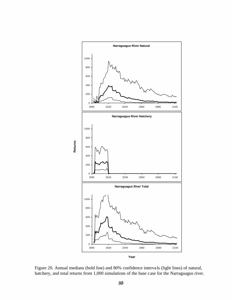
Figure 20. Annual medians (bold line) and 80% confidence interva ls (light lines) of natural,hatchery, and total returns from 1,000 simulations of the base case for the Narraguagus river.

Ret

urn

s

Year

Narraguagus River Natural

0

200

400

600

800

1000

2000 2020 2040 2060 2080 2100

Narraguagus River Hatchery

0

200

400

600

800

1000

2000 2020 2040 2060 2080 2100

Narraguagus River Total

0

200

400

600

800

1000

2000 2020 2040 2060 2080 2100

Figure 21. Annual medians (bold line) and 80% confidence interva ls (light lines) of natural,hatchery, and total returns from 1,000 simulations of the base case for Cove Brook.

Ret

urn

s

Year

Cove Brook Natural

0

5

10

15

20

25

30

2000 2020 2040 2060 2080 2100

Cove Brook Hatchery

0

5

10

15

20

25

30

2000 2020 2040 2060 2080 2100

Cove Brook Total

0

5

10

15

20

25

30

2000 2020 2040 2060 2080 2100

Figure 22. Annual medians (bold line) and 80% confidence interva ls (light lines) of natural,hatchery, and total returns from 1,000 simulations of the base case for all 8 DPS rivers.

Ret

urns

Year

DPS Natural

0

500

1000

1500

2000

2500

3000

3500

4000

2000 2020 2040 2060 2080 2100

DPS Hatchery

0

500

1000

1500

2000

2500

3000

3500

4000

2000 2020 2040 2060 2080 2100

DPS Total

0

500

1000

1500

2000

2500

3000

3500

4000

2000 2020 2040 2060 2080 2100

Figure 23. Replacement rate distributions for all rivers and river groups using base caseinputs and 10,000 simulations. The red bars denote the bin containing 1.0 as its upper bound.

DE

0

500

1000

1500

2000

2500

3000

0 0.5 1 1.5 2Replacement Rate

Fre

qu

ency

0.00

0.25

0.50

0.75

1.00

Cu

mu

lati

ve

EM

0

500

1000

1500

2000

2500

0 0.5 1 1.5 2Replacement Rate

Fre

qu

ency

0.00

0.25

0.50

0.75

1.00

Cu

mu

lati

ve

PL

0

1000

2000

3000

4000

5000

6000

0 0.5 1 1.5 2Replacement Rate

Fre

qu

ency

0.00

0.25

0.50

0.75

1.00

Cu

mu

lati

ve

NG

0

200400

600

800

10001200

1400

0 0.5 1 1.5 2Replacement Rate

Fre

qu

ency

0.00

0.25

0.50

0.75

1.00

Cu

mu

lati

ve

MC

0200400600800

1000120014001600

0 0.5 1 1.5 2Replacement Rate

Fre

qu

ency

0.00

0.25

0.50

0.75

1.00

Cu

mu

lati

ve

CB

010002000300040005000600070008000

0 0.5 1 1.5 2Replacement Rate

Fre

qu

ency

0.00

0.25

0.50

0.75

1.00

Cu

mu

lati

ve

DT

0

1000

2000

3000

40005000

6000

7000

0 0.5 1 1.5 2Replacement Rate

Fre

qu

ency

0.00

0.25

0.50

0.75

1.00

Cu

mu

lati

ve

SHP

0

500

1000

1500

2000

2500

0 0.5 1 1.5 2Replacement Rate

Fre

qu

ency

0.00

0.25

0.50

0.75

1.00

Cu

mu

lati

ve

DPS

0

500

1000

1500

2000

0 0.5 1 1.5 2Replacement Rate

Fre

qu

ency

0.00

0.25

0.50

0.75

1.00

Cu

mu

lati

ve

Downeast

0

500

1000

1500

2000

0 0.5 1 1.5 2Replacement Rate

Fre

qu

ency

0.00

0.25

0.50

0.75

1.00

Cu

mu

lati

ve

Southwest

0

500

1000

1500

2000

2500

0 0.5 1 1.5 2Replacement Rate

Fre

qu

ency

0.00

0.25

0.50

0.75

1.00C

um

ula

tive

Figure 24. Medians of total returns to the DPS when juvenile survival (four thin lines) or average marine survival (line with circles) are increased 20% compared to the base case (thick line).

0

500

1000

1500

2000

2500

3000

3500

2000 2020 2040 2060 2080 2100

Year

Tota

l Ret

urns

to

DP

S

Base Case Juvenile S Inc 20% Marine S Inc 20%

Figure 25. Three separate trajectories of total returns to the DPS (thin lines with symbols)shown relative to the median and 80% confidence interval (thick lines) from the sensitivityanalysis when average marine survival was increased 20%.

0

1000

2000

3000

4000

5000

6000

7000

2000 2020 2040 2060 2080 2100

Year

To

tal

Ret

urn

s to

DP

S

0

1000

2000

3000

4000

5000

6000

7000

2000 2020 2040 2060 2080 2100

Year

To

tal

Ret

urn

s to

DP

S

0

1000

2000

3000

4000

5000

6000

7000

2000 2020 2040 2060 2080 2100

Year

To

tal

Ret

urn

s to

DP

S

Figure 26. Median replacment rate of the DPS as a function of changes in either the averagemarine survival rate or the parr1+ to smolt (juvenile) survival rate.

0.80

0.90

1.00

1.10

0 10 20 30 40 50 60

Relative Increase in Survival (%)

Med

ian

Rep

lace

men

t R

ate

for

DP

S

Marine

Juvenile

Figure 27. Replacement rate distributions for all rivers and river groups using CSE levels forpopulation abundance, increasing average marine survival 35%, and 10,000 simulations. The red bars denote the bin containing 1.0 as its upper bound.

DE

0

500

1000

1500

2000

0 0.5 1 1.5 2Replacement Rate

Fre

qu

ency

0.00

0.25

0.50

0.75

1.00

Cu

mu

lati

ve

EM

0

500

1000

1500

2000

0 0.5 1 1.5 2Replacement Rate

Fre

qu

ency

0.00

0.25

0.50

0.75

1.00

Cu

mu

lati

ve

PL

0

500

1000

1500

2000

0 0.5 1 1.5 2Replacement Rate

Fre

qu

ency

0.00

0.25

0.50

0.75

1.00

Cu

mu

lati

ve

NG

0

500

1000

1500

2000

0 0.5 1 1.5 2Replacement Rate

Fre

qu

ency

0.00

0.25

0.50

0.75

1.00

Cu

mu

lati

ve

MC

0

500

1000

1500

2000

0 0.5 1 1.5 20.00

0.25

0.50

0.75

1.00

CB

0

500

1000

1500

2000

2500

0 0.5 1 1.5 2

0.00

0.25

0.50

0.75

1.00

DT

0

500

1000

1500

2000

0 0.5 1 1.5 2Replacement Rate

Fre

qu

ency

0.00

0.25

0.50

0.75

1.00

Cu

mu

lati

ve

SHP

0

500

1000

1500

2000

0 0.5 1 1.5 2Replacement Rate

Fre

qu

ency

0.00

0.25

0.50

0.75

1.00

Cu

mu

lati

ve

DPS

0

500

1000

1500

2000

0 0.5 1 1.5 2Replacement Rate

Fre

qu

ency

0.00

0.25

0.50

0.75

1.00

Cu

mu

lati

ve

Downeast

0

500

1000

1500

2000

0 0.5 1 1.5 2Replacement Rate

Fre

qu

ency

0.00

0.25

0.50

0.75

1.00

Cu

mu

lati

ve

Southwest

0

500

1000

1500

2000

0 0.5 1 1.5 20.00

0.25

0.50

0.75

1.00

88

Appendix

List of Working Group Participants and Affiliations

Anderson, Marty NMFSBeland, Ken ASCBjorkstedt, Eric NMFSBurger, Carl FWSColligan, Mary NMFSCooney, Tom NMFSHawkes, Jim NMFSHecht, Anne FWSICES WGNAS variousKimball, Dan FWSKinnison, Mike UMaineKocik, John NMFSLegault, Chris NMFSLindley, Steve NMFSMackey, Greg AFSMarancik, Jerry FWSMcElhany, Paul NMFSMinton, Mark NMFSNichols, Henry ASCNickerson, Paul FWSParkin, Mary FWSPerkins, Dave FWSSaunders, Rory NMFSScida, Pat NMFSSheehan, Tim NMFSTrial, Joan ASCWainwright, Tom NMFSWaples, Robin NMFS

ASC = Maine Atlantic Salmon CommissionFWS = US Fish and Wildlife ServiceNMFS = National Marine Fisheries ServiceUMaine = University of MaineWGNAS = Working Group on North Atlantic Salmon

Procedures for Issuing Manuscriptsin the

Northeast Fisheries Science Center Reference Document (CRD) Series

Clearance: All manuscripts submitted for issuance asCRDs must have cleared the NEFSC 's manuscript/abstract/webpage review process. If any author is not a federalemployee, he/she will be required to sign an “NEFSCRelease-of-Copyright Form.” If your manuscript includesmaterial lifted from another work which has been copy-righted, then you will need to work with the NEFSC’sEditorial Office to arrange for permission to use that mate-rial by securing release signatures on the “NEFSC Use-of-Copyrighted-Work Permission Form.”

Organization: Manuscripts must have an abstract and tableof contents, and — if applicable — lists of figures and tables.As much as possible, use traditional scientific manuscriptorganization for sections: “Introduction,” “Study Area”/”Experimental Apparatus,” “Methods,” “Results,” “Dis-cussion” and/or “Conclusions,” “Acknowledgments,” and“Literature/References Cited.”

Style: The CRD series is obligated to conform with the stylecontained in the current edition of the United States Govern-ment Printing Office Style Manual. That style manual issilent on many aspects of scientific manuscripts. The CRDseries relies more on the CBE Style Manual. Manuscriptsshould be prepared to conform with these style manuals.

The CRD series uses the American Fisheries Society’sguides to names of fishes, mollusks, and decapod crusta-ceans, the Society for Marine Mammalogy’s guide to namesof marine mammals, the Biosciences Information Service’sguide to serial title abbreviations, and the InternationalStandardization Organization’s guide to statistical terms.

For in-text citation, use the name-date system. Aspecial effort should be made to ensure that all necessarybibliographic information is included in the list of citedworks. Personal communications must include date, fullname, and full mailing address of the contact.

Preparation: Type a clean/neat, single-spaced version ofthe document, using Microsoft Word or Corel WordPerfect.The document must be paginated continuously from begin-ning to end and must have a “Table of Contents.” Begin thepreliminary pages of the document — always the “Table ofContents” — with page “iii.” Begin the body of the docu-ment — normally the “Introduction” — with page “1,” andcontinuously paginate all pages including tables, figures,appendices, and indices. You can insert blank pages asappropriate throughout the document, but account for themin your pagination (e.g., if your last figure ends on an odd-numbered/right-hand page such as “75,” and if your nextpage is the first page of an appendix, then you wouldnormally insert a blank page after the last figure, andpaginate the first page of the appendix as “77” to make itbegin on an odd-numbered/right-hand page also). Forwardthe final version to the Editorial Office as both a paper copyand electronically (i.e., e-mail attachment, 3.5-inch floppydisk, high-density zip disk, or CD).

Production and Distribution: The Editorial Office willdevelop the inside and outside front covers, the inside andoutside back covers, and the title and bibliographic controlpages (pages “i” and “ii”) of the document, then combinethose covers and preliminary pages with the text that youhave supplied. The document will then be issued online.

Paper copies of the four covers and two preliminarypages will be sent to the sole/senior NEFSC author shouldhe/she wish to prepare some paper copies of the overalldocument as well. The Editorial Office will only producefour paper copies (i.e., three copies for the NEFSC’s librar-ies and one copy for its own archives) of the overall docu-ment.

A number of organizations and individuals in the North-east Region will be notified by e-mail of the availability ofthe online version of the document. The sole/senior NEFSCauthor of the document will receive a list of those so notified.

Research Communications UnitNortheast Fisheries Science Center

National Marine Fisheries Service, NOAA166 Water St.

Woods Hole, MA 02543-1026

Publications and Reportsof the

Northeast Fisheries Science CenterThe mission of NOAA's National Marine Fisheries Service (NMFS) is "stewardship of living marine resources for the benefit of the nationthrough their science-based conservation and management and promotion of the health of their environment." As the research arm of theNMFS's Northeast Region, the Northeast Fisheries Science Center (NEFSC) supports the NMFS mission by "planning, developing, andmanaging multidisciplinary programs of basic and applied research to: 1) better understand the living marine resources (including marinemammals) of the Northwest Atlantic, and the environmental quality essential for their existence and continued productivity; and 2) describeand provide to management, industry, and the public, options for the utilization and conservation of living marine resources andmaintenance of environmental quality which are consistent with national and regional goals and needs, and with internationalcommitments." Results of NEFSC research are largely reported in primary scientific media (e.g., anonymously-peer-reviewed scientificjournals). However, to assist itself in providing data, information, and advice to its constituents, the NEFSC occasionally releases its resultsin its own media. Currently, there are three such media:

NOAA Technical Memorandum NMFS-NE -- This series is issued irregularly. The series typically includes: data reports of long-term field or lab studies of important species or habitats; synthesis reports for important species or habitats; annual reports of overallassessment or monitoring programs; manuals describing program-wide surveying or experimental techniques; literature surveys ofimportant species or habitat topics; proceedings and collected papers of scientific meetings; and indexed and/or annotatedbibliographies. All issues receive internal scientific review and most issues receive technical and copy editing.

Northeast Fisheries Science Center Reference Document -- This series is issued irregularly. The series typically includes: datareports on field and lab studies; progress reports on experiments, monitoring, and assessments; background papers for, collectedabstracts of, and/or summary reports of scientific meetings; and simple bibliographies. Issues receive internal scientific review, butno technical or copy editing.

Resource Survey Report (formerly Fishermen's Report) -- This information report is a quick-turnaround report on the distributionand relative abundance of selected living marine resources as derived from each of the NEFSC's periodic research vessel surveys ofthe Northeast's continental shelf. There is no scientific review, nor any technical or copy editing, of this report.

OBTAINING A COPY: To obtain a copy of a NOAA Technical Memorandum NMFS-NE or a Northeast Fisheries Science CenterReference Document, or to subscribe to the Resource Survey Report, either contact the NEFSC Editorial Office (166 Water St., WoodsHole, MA 02543-1026; 508-495-2228) or consult the NEFSC webpage on "Reports and Publications" (http://www.nefsc.noaa.gov/nefsc/publications/).

ANY USE OF TRADE OR BRAND NAMES IN ANY NEFSC PUBLICATION OR REPORT DOES NOT IMPLYENDORSEMENT.

MEDIA MAIL