SAFETY RISK ASSESSMENT STUDY BASIS Appendix 1 · PDF fileSAFETY RISK ASSESSMENT STUDY BASIS ....

SAFETY RISK ASSESSMENT STUDY BASIS

Appendix 1 Washington State Ferries

Report No. PP061307-02, Rev. 02 Document No.: 167NWYK-13 Date: 2014-06-04

Project name: Safety Risk Assessment Study Basis Det Norske Veritas (U.S.A.), Inc.

DNV GL Oil & Gas Risk Advisory Services 1400 Ravello Dr Suite 100 77449 Katy TX United States Tel: +1 281 396 1000

Report title: Appendix 1 Customer: Washington State Ferries, Contact person: Darnell Baldinelli Date of issue: 2014-06-04 Project No.: PP061307 Organisation unit: Risk Advisory Services Report No.: PP061307-2, Rev. 02 Document No.: 167NWYK-13

DNV GL – Report No. PP061307-2, Rev. 02 – www.dnvgl.com Page i

Abbreviations

BLEVE Boiling Liquid Expanding Vapor Explosion

DNV Det Norske Veritas

ESDV Emergency shutdown valves

FPSO ` Floating Production Storage Offloading

HCRD Hydrocarbon Release Database

LEAK DNV Software used to estimate frequency of failure

LFL Lower Flammable Limit

NCDC National Climatic Data Center

NOAA National Oceanic and Atmospheric Administration

PHAST RISK Process Hazard Analysis Software Tools

P&ID Piping and Instrumentation Diagram

QRA Quantitative Risk Assessment

SEP Surface Emissive Power

UKOOA United Kingdom Offshore Operator Association

UK United Kingdom

ULF Upper Flammable Limit

WSF Washington State Ferries

DNV GL – Report No. PP061307-2, Rev. 02 – www.dnvgl.com Page ii

Units of Measure

°C degrees Celsius

°F degrees Fahrenheit

barg bar gauge

ft feet

gal gallons

hr hours

in. inches

kg kilograms

kJ kilojoules

kW/m2 kilowatts per square meter

m meters

mi miles

min minutes

mm millimeters

psig pounds per square inch gauge

s seconds


Table of contents

INTRODUCTION ........................................................................................................................... 2

1 BACKGROUND DATA ....................................................................................................... 3 1.1 Operational 3 1.2 Population Data 5 1.3 Meteorological Data 11

2 CONSEQUENCE MODELLING PARAMETERS ....................................................................... 13 2.1 Inventory Estimate 13 2.2 Release Angle 13 2.3 Hole Size 14 2.4 Release Location 14 2.5 Release Elevation 14

3 INPUT TO RISK ASSESSMENT ........................................................................................ 15 3.1 Detection and Isolation Times 15 3.2 Ignition Probability 16 3.3 Event Tree Framework 17

4 OPERATIONAL SCENARIO DEFINITION ............................................................................ 18

5 OPERATIONAL LEAK FREQUENCY ANALYSIS ..................................................................... 19 5.1 Tanker and Hose 19 5.2 Hydrocarbon-Containing Process Equipment 20 5.3 Operational Leak Frequency Results 21

6 REFERENCES ................................................................................................................ 22


INTRODUCTION This appendix documents the key assumptions for the Safety Risk Assessment. These assumptions apply to any loss of containment triggered either by an operational or a navigational event. In general, changes to these assumptions have the potential to materially change the outcome of the results.

DNV GL – Report No. PP061307-2, Rev. 02 – www.dnvgl.com Page 2

1 BACKGROUND DATA Background data/assumptions that provided key input to the study are of three basic types:

• Operational (Section 1.1) • Population (Section 1.2) • Meteorological (Section 1.3)

1.1 Operational This section documents the assumptions related to operations (bunkering and transit) that were input to the safety analysis.

1.1.1 Bunkering System Figure 1-1 shows the planned layout of the equipment on the ferry. The portions of the ferry bunkering system relevant for the analysis were defined as:

• LNG trucks. The inventory of an LNG truck is 38.4 m3 (10,145 liquid gal). There will be two LNG trucks for each bunkering. The bunkering flow rate is 0.1 kg/s (transferring 10,000 gal in 45 min).

• One loading hose, assumed to be 10 m (35 ft) in length from the LNG truck to LNG bunkering station. The diameter of the hose is 0.075 m (3 in.).

• Piping on the ferry from bunkering station to the LNG tanks. The diameter of the piping is 0.075 m (3 in.).

• Two LNG tanks on the Texas deck of the LNG ferry. Each of the tanks has a capacity of 100 m3 (26,420 gal). The tanks will be of type double shell vacuum-insulated pressure vessels, with a design pressure of 7.5 barg (109 psig) and an operating pressure of 5 to 6 barg (73 to 87 psig).


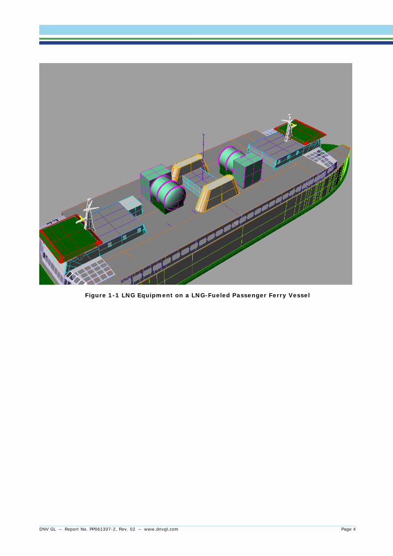
Figure 1-1 LNG Equipment on a LNG-Fueled Passenger Ferry Vessel


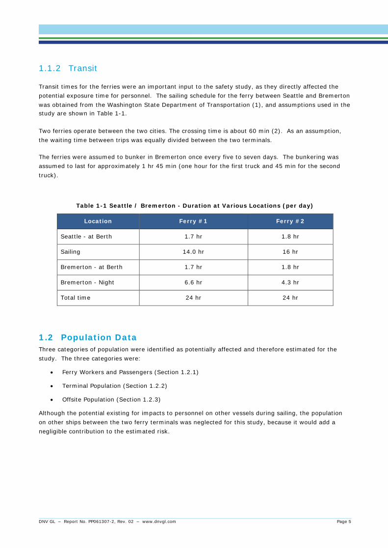
1.1.2 Transit

Transit times for the ferries were an important input to the safety study, as they directly affected the potential exposure time for personnel. The sailing schedule for the ferry between Seattle and Bremerton was obtained from the Washington State Department of Transportation (1), and assumptions used in the study are shown in Table 1-1.

Two ferries operate between the two cities. The crossing time is about 60 min (2). As an assumption, the waiting time between trips was equally divided between the two terminals.

The ferries were assumed to bunker in Bremerton once every five to seven days. The bunkering was assumed to last for approximately 1 hr 45 min (one hour for the first truck and 45 min for the second truck).

Table 1-1 Seattle / Bremerton - Duration at Various Locations (per day)

Location Ferry #1 Ferry #2

Seattle - at Berth 1.7 hr 1.8 hr

Sailing 14.0 hr 16 hr

Bremerton - at Berth 1.7 hr 1.8 hr

Bremerton - Night 6.6 hr 4.3 hr

Total time 24 hr 24 hr

1.2 Population Data Three categories of population were identified as potentially affected and therefore estimated for the study. The three categories were:

• Ferry Workers and Passengers (Section 1.2.1)

• Terminal Population (Section 1.2.2)

• Offsite Population (Section 1.2.3)

Although the potential existing for impacts to personnel on other vessels during sailing, the population on other ships between the two ferry terminals was neglected for this study, because it would add a negligible contribution to the estimated risk.


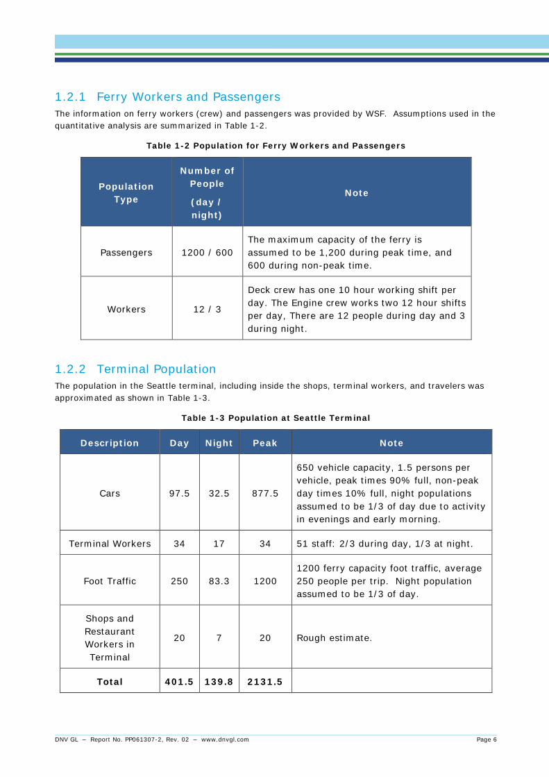
1.2.1 Ferry Workers and Passengers The information on ferry workers (crew) and passengers was provided by WSF. Assumptions used in the quantitative analysis are summarized in Table 1-2.

Table 1-2 Population for Ferry Workers and Passengers

Population Type

Number of People

(day / night)

Note

Passengers 1200 / 600 The maximum capacity of the ferry is assumed to be 1,200 during peak time, and 600 during non-peak time.

Workers 12 / 3

Deck crew has one 10 hour working shift per day. The Engine crew works two 12 hour shifts per day, There are 12 people during day and 3 during night.

1.2.2 Terminal Population The population in the Seattle terminal, including inside the shops, terminal workers, and travelers was approximated as shown in Table 1-3.

Table 1-3 Population at Seattle Terminal

Description Day Night Peak Note

Cars 97.5 32.5 877.5

650 vehicle capacity, 1.5 persons per vehicle, peak times 90% full, non-peak day times 10% full, night populations assumed to be 1/3 of day due to activity in evenings and early morning.

Terminal Workers 34 17 34 51 staff: 2/3 during day, 1/3 at night.

Foot Traffic 250 83.3 1200 1200 ferry capacity foot traffic, average 250 people per trip. Night population assumed to be 1/3 of day.

Shops and Restaurant Workers in Terminal

20 7 20 Rough estimate.

Total 401.5 139.8 2131.5


At Bremerton, the terminal population was estimated based on a review of buildings and their functions at the terminal. The estimated population is shown in Table 1-4. The numbers in Table 1-4 correspond to the numbers in Figure 1-2. The risk results are not strongly affected by the estimates in the below table, because the ferry would not be present at the terminal for a long duration.

Table 1-4 Population at Bremerton Terminal

# Building Day Night Peak Note

1 Kitsap

Conference Center

750 people capacity +

staff 120 0 20

Day average estimated to be 100 + 20 staff in the day. Operates at capacity of 750 + staff at only several peak times (conference peak times and transit peak times not the same). Population consists of only staff at peak transit times. Some activity early in the night is not included since a 12 hour day includes some time without much activity.

2 Hampton

Inn 105 rooms

+ staff 40 83.8 40

75% of 105 room capacity, average 1 person per room, 2 staff during night, 40 staff and guests assumed during day and peak times.

3 Ferry Lanes and

Terminal 302.5 100.8 1528.5

230 vehicle capacity, 1.5 persons per vehicle. Non-peak day 10% full + 18 employees + 250 average foot traffic. Peak times 90% full + 18 employees + 1200 ferry capacity foot traffic. Night is 1/3 of day due to activity in evening and early morning.

4 Navy Museum 15 0 6 Average 12 visitors per day + 3 staff volunteers

5 Five Storefront

Restaurants and Shops 20 5 20

Average 5 staff at night and 20 people during day and peak time

6 Easton College and a

Credit Union 150 2 60

Enrollment of 120 + staff + credit union staff

Total 612.5 191.6 1633.5


Figure 1-2 Bremerton Terminal Population Centers


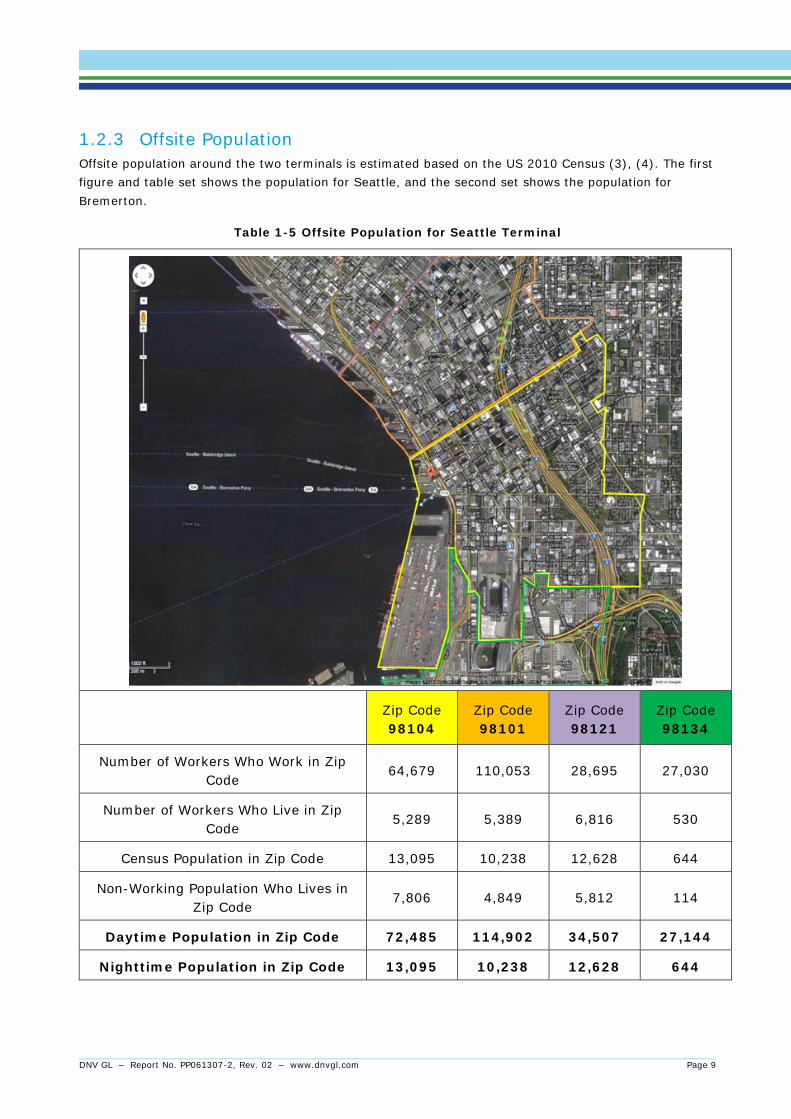
1.2.3 Offsite Population Offsite population around the two terminals is estimated based on the US 2010 Census (3), (4). The first figure and table set shows the population for Seattle, and the second set shows the population for Bremerton.

Table 1-5 Offsite Population for Seattle Terminal

Zip Code 98104

Zip Code 98101

Zip Code 98121

Zip Code 98134

Number of Workers Who Work in Zip Code

64,679 110,053 28,695 27,030

Number of Workers Who Live in Zip Code

5,289 5,389 6,816 530

Census Population in Zip Code 13,095 10,238 12,628 644

Non-Working Population Who Lives in Zip Code

7,806 4,849 5,812 114

Daytime Population in Zip Code 72,485 114,902 34,507 27,144

Nighttime Population in Zip Code 13,095 10,238 12,628 644


Table 1-6 Offsite Population for Bremerton Terminal

Zip Code 98310

Zip Code 98337

Zip Code 98314

Number of Workers Who Work in Zip Code

6,273 4,213 191

Number of Workers Who Live in Zip Code

6,726 2,217 219

Census Population in Zip Code 18,703 6,697 3,329

Non-Working Population Who Lives in Zip Code

11,977 4,480 3,110

Daytime Population in Zip Code 18,250 8,693 3,301

Nighttime Population in Zip Code 18,703 6,697 3,329


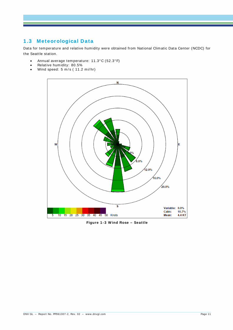
1.3 Meteorological Data Data for temperature and relative humidity were obtained from National Climatic Data Center (NCDC) for the Seattle station.

• Annual average temperature: 11.3°C (52.3°F) • Relative humidity: 80.5% • Wind speed: 5 m/s ( 11.2 mi/hr)

Figure 1-3 Wind Rose – Seattle


Figure 1-4 Wind Rose - Bremerton


2 CONSEQUENCE MODELLING PARAMETERS For consequence modeling the widely-accepted PHAST RISK default values were applied in general. For purposes of documentation of the model, the project-specific key parameters for the consequence models in PHAST are summarized below:

• Jet fire – maximum surface emissive power: 250 kW/m2 • Jet fire – rate modification factor (the mass of vapor that remains in cloud calculated by PHAST

is multiplied by this factor – determines the proportion of the liquid fraction that contributes to the jet fire for 2-phase jets): 3

• Pool fire – minimum duration – 10 seconds • Fireball / BLEVE – maximum surface emissive power: 300 kW/m2 • Fireball / BLEVE – mass modification factor (the mass of vapor that remains in the cloud

calculated by PHAST is multiplied by this factor – determines the proportion of the liquid fraction that contributes to a fireball/BLEVE): 3

• Flash fire – The size is calculated based on mass between lower flammable limit and upper flammable limit (for ignition probabilities, the 50% lower flammable limit was used)

• Explosion – minimum explosion energy: 5 x 106 kJ • Explosion – explosion efficiency: 10%

The key inputs to determine the source terms or discharge conditions are presented in following sections.

2.1 Inventory Estimate An estimate of the inventory that could potentially be released was developed for each isolatable section. The estimate of total released inventory (IT) was the sum of IS (Static Inventory, kg) and ID (Dynamic Inventory, kg). The static inventory was the amount of material within the isolatable section's vessels and piping, prior to a leak. The dynamic inventory was calculated based on the pumped-in flow rate and the isolation time by:

trrMINII PLST •+= ),()()(

Total potential inventory released (kg)

Static inventory (kg)

Leak rate (kg/s)

Process flow rate (kg/s)

Release duration (s)

2.2 Release Angle Most of the releases were assumed to be in the horizontal direction. Two types of scenarios were assumed to be released at different angles:

• Vent release: vertical,

• LNG tank on ferry and truck tank release: downward impinged.

=====

trrII

P

L

S

T

)(

)(


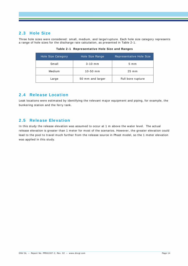
2.3 Hole Size Three hole sizes were considered: small, medium, and large/rupture. Each hole size category represents a range of hole sizes for the discharge rate calculation, as presented in Table 2-1.

Table 2-1 Representative Hole Size and Ranges

Hole Size Category Hole Size Range Representative Hole Size

Small 3-10 mm 5 mm

Medium 10-50 mm 25 mm

Large 50 mm and larger Full bore rupture

2.4 Release Location Leak locations were estimated by identifying the relevant major equipment and piping, for example, the bunkering station and the ferry tank.

2.5 Release Elevation In this study the release elevation was assumed to occur at 1 m above the water level. The actual release elevation is greater than 1 meter for most of the scenarios. However, the greater elevation could lead to the pool to travel much further from the release source in Phast model, so the 1 meter elevation was applied in this study.


3 INPUT TO RISK ASSESSMENT The technical details of modeling LNG require three specialized inputs that relate to how long a leak might continue before the equipment is isolated, whether the material ignites (either before or after a vapor cloud forms), and how the previous two interrelate in the model.

The following key parameters in the PHAST RISK model describe how the model deals with the above issues:

• Detection and Isolation Times (Section 3.1) • Ignition Probability (Section 3.2) • Event Tree Framework (Section 3.3)

3.1 Detection and Isolation Times The times required to detect a release of gas and then to initiate isolation are summarized in this section, which give the representative times assumed for two modes of operation: LNG bunkering and normal operations.

During bunkering operations, it is assumed that an operator is present and watchful during bunkering. It is assumed therefore that an LNG release will be detected and isolated within 1 minute.

During normal sailing operations, it is assumed that operations personnel will have other duties, and the primary means of detection of a “smaller” leak will be either observation by a passenger / crewmember, or alarm of a gas detector. It is anticipated that the detector layout will not be as comprehensive on the vessel as it would be on a typical onshore LNG plant. Given these assumptions, typical detection times for the general process plants were applied to this study, rather than a typical LNG plant, because of the anticipated detection and isolation philosophy and systems on the ferry vessels.

The following values were assumed for this study:

• Small release (3-10 mm hole), 30 min to detect and isolate • Medium release (10-50 mm hole), 15 min to detect and isolate • Large release (>50 mm hole), 5 min to detect and isolate


3.2 Ignition Probability Should an LNG release occur from an LNG tank or instrumentation (such as a pressure gauge, valves, or piping), LNG would quickly vaporize in the ambient air. LNG is natural gas (methane) under normal temperature conditions. Unignited methane is buoyant, and will naturally rise and can disperse to a safe (nonflammable) concentration.

Immediate ignition occurs when the fluid ignites immediately upon release due to auto-ignition or because the cause of the release also provides an ignition source. Delayed ignition is the result of a build-up of a flammable vapor cloud, ignited by a source that is remote from the release point. Delayed ignition can result in a flash fire or explosion, and may also burn back to the leak source resulting in a jet fire and/or pool fire.

Immediate ignition of a release was modeled as having a constant (but small) ignition probability. Immediate ignition often has a smaller impact footprint than late ignition, because a flammable cloud has not had time to fully form. A probability of 1 in 1,000 was applied in the model to account for immediate ignition due to friction and turbulence of fluid releases.

Delayed ignition was modeled as a probability function rather than a constant value, like early ignition. Delayed ignition was a function of the average hole size, phase released, operating conditions, and ignition classification of the area.

Ignition probabilities published by the International Association of Oil and Gas Producers (OGP) (5) were applied in this study, because the offshore industry has more extensive data pertaining to ignited leaks than the maritime industry. Based on the available OGP models, the "UKOOA - Scenario 24 FPSO Gas" model was considered to be best suited for this analysis, especially since the released LNG would propagate on an open deck, similarly to a comparable leak on a large LNG ship.

Table 3-1 Immediate plus Delayed Ignition Probabilities (5)

Release Rate (kg/s)

Ignition Probability

0.1 0.0010

0.2 0.0011

0.5 0.0012

1 0.0013

2 0.0030

5 0.0092

10 0.0213

20 0.0493

50 0.1500

100 0.1500

200 0.1500

500 0.1500

1000 0.1500


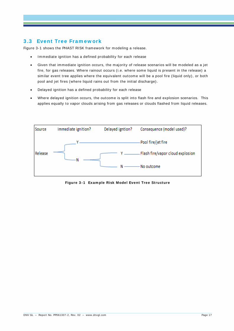
3.3 Event Tree Framework Figure 3-1 shows the PHAST RISK framework for modeling a release.

• Immediate ignition has a defined probability for each release

• Given that immediate ignition occurs, the majority of release scenarios will be modeled as a jet fire, for gas releases. Where rainout occurs (i.e. where some liquid is present in the release) a similar event tree applies where the equivalent outcome will be a pool fire (liquid only), or both pool and jet fires (where liquid rains out from the initial discharge).

• Delayed ignition has a defined probability for each release

• Where delayed ignition occurs, the outcome is split into flash fire and explosion scenarios. This applies equally to vapor clouds arising from gas releases or clouds flashed from liquid releases.

Figure 3-1 Example Risk Model Event Tree Structure


4 OPERATIONAL SCENARIO DEFINITION Release scenarios (failure cases) were defined using a specific set of conditions to characterize a range of possible conditions of failure. It was not practicable or necessary to consider every possible permutation of release rate (or hole size) and location, precise inventory at time of failure, temperature, pressure etc., since during a real event, all of these vary continuously between limits. Thus, characteristic values of each parameter to model the failure were selected in such a way as to cover the spectrum of possible values. A total of 22 process release scenarios were defined.

Table 7-1 summarizes the scenarios and process conditions modeled in the quantitative risk assessment (QRA). The static inventory estimate presented in the table was obtained by calculating the volume within each isolatable section. The length of the piping within the section was estimated based on the equipment arrangement drawings, while the diameter of the piping was noted from the Piping and Instrumentation Diagrams (P&IDs).

Note that the total released inventory for each release case was estimated taking into account the release rate, detection and isolation times, along with the static inventory.


5 OPERATIONAL LEAK FREQUENCY ANALYSIS The methodology used to estimate the leak frequency during operation is described in this section. The frequency estimate was conducted by applying two approaches to obtain the best possible assessment of the potential for a leak of a given size:

1. Frequency of a leak during loading (Section 4.1 Tanker and Hose)

2. Frequency of a leak from the hydrocarbon-containing equipment on the vessel (Section 4.2 Hydrocarbon-Containing Process Equipment)

5.1 Tanker and Hose

Failure frequencies for flexible unloading hoses and tanks on moving vehicles were taken from the Purple Book (6). The “Coloured Books” are used around the world as standard reference material in safety studies. The Purple Book, Guidelines for quantitative risk assessment (6), documents standard methods to calculate the risks due to dangerous substances using available models and data. Data from unloading truck was modified by the operational presence factor. The hose frequency was multiplied by the number of unloading hours per year.

Table 4-1 Summary of Unloading Equipment Frequencies

Scenario Description

Road Tanker in an

Establishment Leak Frequency

(per year)

Flexible Hose Leak Frequency

(per hour)

Continuous release from a hole the size of the largest connection 5.0x10-7 4.0x10-5 Instantaneous release of the complete inventory 5.0 x10-7 4.0x10-6

Total 1.0x10-6 4.4x10-5


5.2 Hydrocarbon-Containing Process Equipment The basis for a definition of representative leak scenarios requires estimation of the leak frequency contribution from each release scenario.

DNV’s commercial software LEAK version 3.2.1 was used to estimate leak frequencies. The program contains leak statistics from the Hydrocarbon Release Database (HCRD) published by the United Kingdom (UK) Health and Safety Executive (7). Failure frequencies were estimated based on the hole size ranges presented in Table 4-2.

Table 4-2 Release Rate Distribution for Frequency Analysis

Size Category Hole Size Range (mm)

used for frequency analysis

Representative Hole Size (mm)

Small 3 to 10 5

Medium 10 to 50 25

Large Greater than 50 Full bore rupture

The HCRD data is considered one of the best compilations of loss of containment data for process equipment publicly available, and is collected from offshore platforms in the UK sector of the North Sea. It has become the industry-standard source of leak frequencies for offshore QRA and can be adjusted for onshore QRA. Therefore, the HCRD data are applied in this study as the basis for estimation of the frequency of equipment leaks.

The P&IDs were reviewed to determine appropriate isolation points and identify the process equipment within each isolatable section. An isolatable section was defined as all equipment between emergency shutdown valves (ESDVs), and delineates the maximum inventory available for release assuming that shutdown will be initiated should a release occur.

Each part, as it was counted from P&IDs, was classified by type, size, isolatable segment, and scenario reference. Each part was entered into LEAK in order to estimate the leak frequency for the three different release sizes (small, medium, large). Table 4-2 presents the hole size and distribution assumptions that were applied to each scenario, as relevant.


5.3 Operational Leak Frequency Results The annual leak frequency distribution by scenario is presented in Table 4-3 below. The size of the release is defined as small (S), medium (M), and large (L), each referring to the hole size range from previous Table 4-2.

Table 4-3 Leak Frequency Distribution by Scenario

Category Scenario Description

Hole Size (mm)

Frequency (/yr)

Bunkering

LNG Truck Tank

Catastrophic rupture

released in 1 min 1.2.E-08

Continuous release 75 1.2.E-08

Hose Full bore rupture 75 8.4.E-04 Leak 7.5 8.4.E-04

Bunkering Station - LNG Large 75 1.5.E-06 Medium 25 4.0.E-06 Small 5 8.5.E-06

Bunkering Station - Vapor Return

medium 25 5.3.E-06 Small 5 8.1.E-06

LNG Loading Pipe Large 75 3.7.E-06 Medium 25 7.0.E-06 Small 5 1.7.E-05

Vapor Return Pipe Medium 25 1.5.E-05 Small 5 2.4.E-05

Normal Operation

- Gas Supply

LNG Ferry Tank

Catastrophic rupture

released in 1 min 7.7.E-07

Continuous release 75 7.7.E-07

Gas Supply from Cold Box to Engine Room

Large 63.5 5.1.E-05 Medium 25 5.8.E-05 Small 5 1.5.E-04

Supply Pipe Large 63.5 1.8.E-04 Medium 25 3.0.E-04 Small 5 7.5.E-04

1 estimated release frequency while ferry is at berth, see the Navigational Risk Section for release frequency during transit


6 REFERENCES /1/ Washington State Department of Transportation, Washington State Ferries. Sailing

Schedules (Winter 2013, Spring 2013, Summer 2012, Fall 2012). 2. Washington State Ferries (WSF) Route Reference Book (Appendix P to the Terminal Design Manual M 3082, June 2012). June 2006.

/2/ Washington State Ferries (WSF) Route Reference Book (Appendix P to the Terminal Design Manual M 3082, June 2012). June 2006.

/3/ U.S. Census Bureau, Center for Economic Studies. On the Map. [Online] 2010. http://onthemap.ces.census.gov/.

/4/ United States Census 2010. 2010 Census Data. Census Population Data by Zip Code. [Online] 2010. http://www.census.gov/geo/www/gazetteer/files/Gaz_zcta_national.txt.

/5/ International Association of Oil and Gas Producers (OGP). Risk Assessment Data Directory. March 2010. Report No. 434 -6.1.

/6/ Washington State Ferries (WSF). WSF LNG Concept of Operations (CONOPS) v.3.

/7/ VROM Ministerie van Verkeer en Waterstaat. TNO Purple Book CPR 18 Guidelines fo Quantitative Risk Assessment Part One: Establishments. 3. 2009. Vol. CPR 18. Publication Series on Dangerous Substances (PGS 3).

/8/ UK Health and Safety Executive (HSE). Hydrocarbon Release Database (HCRD). October 1992 - March 2010.


About DNV GL Driven by our purpose of safeguarding life, property and the environment, DNV GL enables organizations to advance the safety and sustainability of their business. We provide classification and technical assurance along with software and independent expert advisory services to the maritime, oil and gas, and energy industries. We also provide certification services to customers across a wide range of industries. Operating in more than 100 countries, our 16,000 professionals are dedicated to helping our customers make the world safer, smarter and greener.

SAFETY RISK ASSESSMENT STUDY BASIS Appendix 1 · PDF fileSAFETY RISK ASSESSMENT STUDY BASIS ....

Documents

Transcript of SAFETY RISK ASSESSMENT STUDY BASIS Appendix 1 · PDF fileSAFETY RISK ASSESSMENT STUDY BASIS ....