Safety Externalities of SUVs on Passenger Cars: An ... · Safety Externalities of SUVs on Passenger...

Safety Externalities of SUVs on Passenger Cars: An Analysis Of the Peltzman Effect Using

FARS Data

By David R. Martinelli, Ph.D., and Maria-Paulina Diosdado-De-La-Pena

West Virginia University

Technical Report Documentation Page 1. Report No. WVU-2006-02

2. Government Accession No. 3. Recipient’s Catalog No. 5. Report Date May 2008

4. Title and Subtitle Safety Externalities of SUVs on Passenger Cars: An Analysis of the Peltzman Effect Using FARS Data

6. Performing Organization Code

7. Author(s) David Martinelli, Maria-Paulina Diosdada-De-La-Pena

8. Performing Organization Report No. 10. Work Unit No. (TRAIS)

9. Performing Organization Name and Address West Virginia University PO Box 6103 Morgantown, WV 26505

11. Contract or Grant No. DTRS99-G-0003

13. Type of Report and Period Covered Final

12. Sponsoring Agency Name and Address WVDOH 1900 Kanawha Blvd Charleston, WV 25305

14. Sponsoring Agency Code

15. Supplementary Notes COTR: 16. Abstract The sport utility vehicle (SUV) is a combination of a light pick up chassis of a passenger car (PC) with the space of a minivan. SUVs have been present in the American market since the 1980s, but it wasn’t until the 1990s that they became popular among consumers. With the growing popularity of the SUV, several issues have been raised. In 2003, Dr. Jeffery Runge, head of the U.S. National Highway Traffic Safety Administration (NHTSA), stated that due to the high roll over rate, this type of vehicle is very dangerous. In addition to the roll over rate, issues like road incompatibility and high gas consumption have also become concerns. Perhaps the biggest anxiety is driver behavior. The driver may have a sense of false security in a bigger vehicle, and therefore, take more risks while driving, which in turn could cause more accidents. 17. Key Words SUVs, safety, passenger cars, fatality crashes, SUVs driver’s behavior, FARS, SUVs characteristics, SUVs inertial properties

18. Distribution Statement No restrictions. This document is available from the National Technical Information Service, Springfield, VA 22161

19. Security Classif. (of this report) Unclassified

20. Security Classif. (of this page) Unclassified

21. No. of Pages 78

22. Price

Safety Externalities of SUVs on Passenger Cars: An Analysis of the Peltzman Effect Using FARS Data

David R. Martinelli, PhD. Maria-Paulina Diosdado-De-La-Pena

Department of Civil and Environmental Engineering Morgantown, West Virginia

2008

Keywords: Transportation, Safety Externalities, Sport Utility Vehicles,

Passenger Cars, Peltzman Effect.

ii

ABSTRACT

Safety Externalities of SUVs on Passenger Cars: An Analysis of the Peltzman Effect Using FARS Data

Maria-Paulina Diosdado-De-La-Pena

In the last decade, Sport Utility Vehicles (SUVs) have become a considerable percentage of the US vehicular fleet, giving rise to several highway safety issues such as: vehicular incompatibility, rollover propensity and offsetting driver behavior. While greater mass, stiffness and dimensions of SUVs relative to passenger cars, are safety advantages of SUVs, they may encourage SUV drivers to engage in a trade off between this new level of safety and risk taking behavior, named Peltzman Effect.

In this research a model developed by Levitt and Poter (2001) for drinking drivers is applied to assessing the Peltzman Effect of SUVs and Passenger Cars with a set of data characteristics to control for preexisting risk taking behavior. It was found that indeed SUVs pose an externality hazard on passenger cars and that SUV drivers are 2.7 times more likely to cause a fatal crash compared to passenger cars.

v

TABLE OF CONTENT ABSTRACT……………………………………………………………………………...ii TABLE OF CONTENTS………………………………………………….…………….v LIST OF FIGURES………………………………………………..…………………...vi LIST OF TABLES………………………………………………………………………vi CHAPTER 1. INTRODUCTION………………………………………………………1 1.1 Background…………………………………………………………………....….…1 1.2 Problem definition…………………………………………………….………….....4 1.3 Objective of the project……………………………………………………………..4

CHAPTER 2. LITERATURE REVIEW………………………………………………6 2.1 Sport Utility Vehicle Characteristics………………………………………………6 2.2 SUVs’ Driver Characteristics………………………………………………………7 2.3 Fatality Analysis Reporting System……………………………………………….8 2.4 Related Studies……………………………………………………………………..9 2.5 The Peltzman Effect………………………………………………………………10

CHAPTER 3. MODEL AND DATA SELECTION…………………………………14 3.1 Problem similarities with the drinking drivers’ analysis of Levitt and Poter....14 3.2 Assumptions of the model……………………………………………………..…15 3.3 Model deduction…………………………………………………………………..16 3.4 Scope and limitations of the model……………………………………………...22 3.5 Data characteristics……………………………………………………………….22 3.6 Selected data………………………………………………………………………24

CHAPTER 4. RESULTS……………………………………………………………..28 4.1 Mid-Atlantic Region ……………………………………………………………...33 4.2 Mid-West Region…………………………………………….…………………...34 4.3 New England Region…………………………………………..………………...35 4.4 South Region……………………………………………………………………...36 4.5 Texas (Case 1 and 2) …………………………………………………………...37 4.6 West Coast Region………………………………………….…………………...39

CHAPTER 5. CONCLUSIONS………………………………………………………44 5.1 Findings…………………………………………………………………………….45 5.2 Future Research…………………………………………………………………..46

REFERENCE LIST……………………………………………………………………47 APPENDIX A. ELEMENTS OF HESSIAN MATRIX………………………………51 APPENDIX B. STATE AND COUNTY CODES………………………………...….53 APPENDIX C. DRIVER TYPE CONFIGURATIONS…………………………..…..73

vi

LIST OF FIGURES Figure 1.1 SUVs sold 1990-2006…………………………………………………..….2 Figure 4.1 Mid-Atlantic Region Fatal Crash Trends……………………………..…29 Figure 4.2 Mid-West Region Fatal Crash Trends…………………………………..30 Figure 4.3 New England Region Fatal Crash Trend……………………………….30 Figure 4.4 South Region Fatal Crash Trends................................................…...31 Figure 4.5 Texas Fatal Crash Trends (Case 1)………………………………….…31 Figure 4.6 Texas Fatal Crash Trends (Case 2)…………………………………….32 Figure 4.7 West Coast Region Fatal Crash Trends…………………………….….32 Figure 4.8 Relatively Likelihood θ for Mid-Atlantic Region……………………..…33 Figure 4.9 Relatively Likelihood θ for Mid-West Region……………………….….34 Figure 4.10 Relatively Likelihood θ for New England Region………………….…35 Figure 4.11 Relatively Likelihood θ for South Region……………………………..36 Figure 4.12 Relatively Likelihood θ for Texas (Case 1)…………………………...37 Figure 4.13 Relatively Likelihood θ for Texas (Case 2)…………………………...38 Figure 4.14 Relatively Likelihood θ for West Coast Region………………………39

LIST OF TABLES Table 1.1 Motor vehicle crash fatalities per year (Source, FARS)………………..2 Table 1.2 Fatal motor vehicle crashes (Source, FARS)…………………………….2 Table 1.3 Sport Utility Vehicles Sold 1980-2006………………………………….…3 Table 3.6.1 Mid-Atlantic Region Two-Car Fatal Crashes………………………….25 Table 3.6.2 Mid-West Region Two-Car Fatal Crashes…………………………….25 Table 3.6.3 New England Region Two-Car Fatal Crashes………………………..25 Table 3.6.4 South Region Two-Car Fatal Crashes……………………………..….26 Table 3.6.5 Texas Two-Car Fatal Crashes (Case 1. Table)……………………...26 Table 3.6.6 Texas Two-Car Fatal Crashes (Case 2. Table)……………………...26 Table 3.6.7 West Coast Region Two-Car Fatal Crashes ………………………...27 Table 4.1 Mid-Atlantic Region Results…………………….……………………..….40 Table 4.2 Mid-West Region Results…………………………………………………40 Table 4.3 New England Region Results…………………………………………….41 Table 4.4 Texas Results (Case 1)…………………………………………………...41 Table 4.5 Texas Results (Case 2)………………………………………………...…42 Table 4.6 South Region Results……………………………………………………..42 Table 4.7 West Coast Region Results………………………………………………43

1

1. INTRODUCTION

1.1 Background

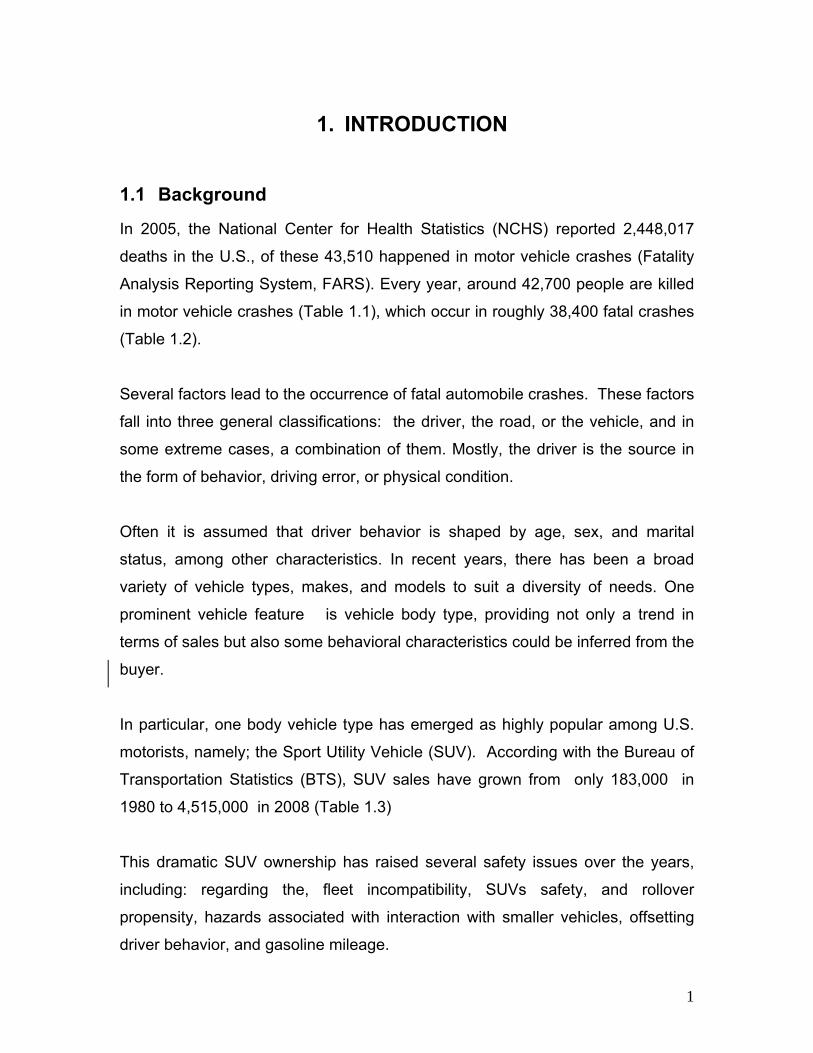
In 2005, the National Center for Health Statistics (NCHS) reported 2,448,017

deaths in the U.S., of these 43,510 happened in motor vehicle crashes (Fatality

Analysis Reporting System, FARS). Every year, around 42,700 people are killed

in motor vehicle crashes (Table 1.1), which occur in roughly 38,400 fatal crashes

(Table 1.2).

Several factors lead to the occurrence of fatal automobile crashes. These factors

fall into three general classifications: the driver, the road, or the vehicle, and in

some extreme cases, a combination of them. Mostly, the driver is the source in

the form of behavior, driving error, or physical condition.

Often it is assumed that driver behavior is shaped by age, sex, and marital

status, among other characteristics. In recent years, there has been a broad

variety of vehicle types, makes, and models to suit a diversity of needs. One

prominent vehicle feature is vehicle body type, providing not only a trend in

terms of sales but also some behavioral characteristics could be inferred from the

buyer.

In particular, one body vehicle type has emerged as highly popular among U.S.

motorists, namely; the Sport Utility Vehicle (SUV). According with the Bureau of

Transportation Statistics (BTS), SUV sales have grown from only 183,000 in

1980 to 4,515,000 in 2008 (Table 1.3)

This dramatic SUV ownership has raised several safety issues over the years,

including: regarding the, fleet incompatibility, SUVs safety, and rollover

propensity, hazards associated with interaction with smaller vehicles, offsetting

driver behavior, and gasoline mileage.

2

Table 1.1 Motor vehicle crash fatalities per year (Source, FARS)

Year 2006 2005 2004 2003 2002 2001 2000 Total

Fatalities 42,642 43,510 42,836 42,884 43,005 42,196 41,945

Table 1.2 Fatal motor vehicle crashes (Source, FARS)

Year 2006 2005 2004 2003 2002 2001 2000 Fatal Motor

Vehicle Crashes

38,588 39,252 38,444 38,477 38,491 37,862 37,526

0

500

1000

1500

2000

2500

3000

3500

4000

4500

5000

1990 1991 1992 1993 1994 1995 1996 1997 1998 1999 2000 2001 2002 2003 2004 2005 2006

Year

SUV

s so

ld (T

hous

ands

of U

nits

)

Figure 1.1 SUVs sold 1990-2006

(Source, Bureau of Transportation Statistics)

3

Table 1.3 Sport Utility Vehicles Sold 1980-2006 (Source, Bureau of Transportation Statistics)

Year Thousands of Units Sold

1980 1985 1990 1991 1992 1993 1994 1995 1996 1997 1998 1999 2000 2001 2002 2003 2004 2005 2006

Small SUV 60 115 189 136 129 144 188 189 120 489 316 314 400 390 354 264 338 172 104 Midsize SUV 100 563 447 904 799 1038 1265 1397 1528 1401 1623 1762 1863 1944 1802 2093 2318 2161 2440 Large SUV 23 57 72 54 75 129 169 230 241 560 642 754 879 1115 2034 1760 1992 2109 1971 T O T A L 183 735 708 1094 1003 1311 1622 1816 1889 2450 2581 2830 3142 3449 4190 4117 4648 4442 4515

4

1.2 Problem definition

Based on BTS data, it can be stated that there has been a considerable increase

of SUVs presence in the U.S. vehicle fleet. This change has introduced two main

safety issues: 1) vehicle incompatibility and 2) offsetting driver behavior. It is refer

by vehicle incompatibility to the different vehicle characteristics as mass, stiffness

and dimensions (Gabler and Hollowell, 1998) that provide uneven protection for

the vehicles involve in case that a motor vehicle crash occurs (Abdelwahab and

Abdel-Aty, 2004).

A common justification of ownership among SUV drivers is the increased (or

perceived increase) in safety achieved through additional weight, stronger

suspension, and higher seating position. This may lead to a false sense of

security among SUV drivers that may result in driving behavior that could pose

increased risks among conventional automobiles. This offsetting driver behavior

is known as the Peltzman Effect, where consumers of a good (in this case SUVs)

pose an externality on non-users (in this case conventional automobiles).

The main issue is to determine if SUVs drivers take greater risks, and translating

this risk to occupants of non-SUVs passenger car occupants. By looking at only

the overall death rates, misleading results maybe obtained because a

confounded effect between vehicle incompatibility and diver behavior is very

likely to exist. While more deaths are expected to occur in passenger cars due to

a structural disadvantage relative to SUVs, it is expected that SUV drivers may

have different driver behavior patterns. This is why it is necessary to develop a

method that separates the effect of SUV driver behavior from that of the vehicle

physical configuration and characteristics.

1.3 Objective of the project

The main objective of this project is to determine if SUV drivers pose safety

externalities on passenger cars, due to an assumed SUV driver offsetting

5

behavior (Peltzman effect). To accomplish this objective it is necessary compete

the following stages,

1) To review the different crash characteristics aspects between SUVs in car

crashes as driver and vehicle characteristics, available crash data, and

Peltzman effect through a comprehensive literature review.

2) To extend existing models of driver behavior to apply to SUVs drivers.

3) To determine the desired data set characteristics and to select the data in

function of those considerations.

4) To apply an appropriate model to the selected data set.

5) To interpret the parameters obtained from the previous stage and

determine if indeed SUVs drivers are more dangerous than the passenger

car drivers, and the statistical significance of those results.

6

2. LITERATURE REVIEW

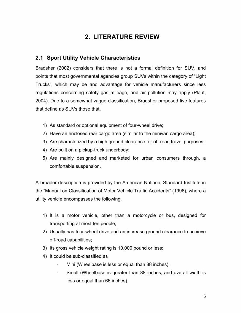
2.1 Sport Utility Vehicle Characteristics

Bradsher (2002) considers that there is not a formal definition for SUV, and

points that most governmental agencies group SUVs within the category of “Light

Trucks”, which may be and advantage for vehicle manufacturers since less

regulations concerning safety gas mileage, and air pollution may apply (Plaut,

2004). Due to a somewhat vague classification, Bradsher proposed five features

that define as SUVs those that,

1) As standard or optional equipment of four-wheel drive;

2) Have an enclosed rear cargo area (similar to the minivan cargo area);

3) Are characterized by a high ground clearance for off-road travel purposes;

4) Are built on a pickup-truck underbody;

5) Are mainly designed and marketed for urban consumers through, a

comfortable suspension.

A broader description is provided by the American National Standard Institute in

the “Manual on Classification of Motor Vehicle Traffic Accidents” (1996), where a

utility vehicle encompasses the following,

1) It is a motor vehicle, other than a motorcycle or bus, designed for

transporting at most ten people;

2) Usually has four-wheel drive and an increase ground clearance to achieve

off-road capabilities;

3) Its gross vehicle weight rating is 10,000 pound or less;

4) It could be sub-classified as

- Mini (Wheelbase is less or equal than 88 inches).

- Small (Wheelbase is greater than 88 inches, and overall width is

less or equal than 66 inches).

7

- Midsize (Wheelbase is greater than 88 inches, and overall width is

greater than 66 inches but less than 75 inches).

- Full-size (Wheelbase is greater than 88 inches, and overall width

is greater or equal than 75 inches but less or equal than 80

inches).

- Large (Wheelbase is greater than 88 inches, and overall width is

greater than 80 inches).

Two SUV characteristics noted above are particularly relevant to this study.

First, they are narrower and higher than other motor vehicles which could lead to

higher rollover potential, and therefore driver injury. Nevertheless, this might be

mitigated by their greater mass and consequently crashworthiness (Khattak and

Rocha, 2003). Second SUVs have greater structural stiffness, since in general, a

stiff frame rail is used instead of unibody (which is a softer design) of passenger

cars (Gabler and Hollowell, 1998).

2.2 SUVs’ Driver Characteristics

Several studies have been conducted to explain driver characteristics as they

relate to vehicle body type. One study established that several aspects such as

travel attitude, personality, and lifestyle are strong factors affecting vehicle type

choice, and in the case of SUVs drivers, these factors were characterized as a

free-spirit attitude (Choo and Mokhtarian, 2004).

Plaut (2004) examined SUV commuters’ characteristics within the framework of

light trucks, through the analysis of the 2001 American Housing Survey,

particularly Journey-to-Work data to determine socio-demographic

characteristics. The findings of the study were that,

8

1) SUV owners take longer trips; in terms of distance an average of 2.4 miles

more and referring time, an average of 1.98 minutes more than car

commuters;

2) SUV owners are more likely to have college education than car

commuters, but less likely to hold postgraduate degrees;

3) SUV owners have incomes that are higher, but their household income is

lower than car commuters;

4) SUV owners surprisingly, own fewer motor vehicles than car commuters.

5) SUV owners are more likely to live close to green areas than urbanized

areas, than car commuters.

6) SUV owners tend to live in rural areas within the MSA, or completely

outside the MSA .

2.3 Fatality Analysis Reporting System

The National Center for Statistics and Analysis (NCSA) of the National Highway

Traffic Safety Administration (NHTSA) created the Fatality Analysis Reporting

System (FARS) in 1975 with the idea of providing a quantitative tool to assess

the safety of the U.S. highway network. The agencies specifically, address

issues such as traffic safety problems and the evaluation of special motor vehicle

and highway safety programs. FARS includes data from fatal traffic crashes

within 50 States, the District of Columbia, and Puerto Rico. For a crash to be

considered in this dataset it must occur in a traffic way open to the public and as

a consequence, the death of one of the people involved in the crash within the

next 30 days. Among the information gathered for FARS are the crash, vehicle,

driver, and person forms (NHTSA and NCSA, “Fatal Crash Data Overview

Brochure).

The crash form includes information regarding the number of fatalities in the

crash, number of vehicle forms submitted, date, atmospheric conditions, and

location where it occurred. The vehicle form includes body type, number of

9

occupants, number of fatalities, travel speed, vehicle year, model and make. The

driver form mainly data about driver license compliance and restrictions, previous

DUIs and previous traffic violations. The person form gathers the characteristics

of the persons involved in the crashes such as age, alcohol presence, injury

severity suffered, sex, seating position and person type.

2.4 Related Studies

Based on the premise that a significant amount of fatalities occur in crashes

involving a light truck or a van (LTV) Gabler and Hollowell (1998) performed a

study to determine if indeed LTVs were more likely to cause more fatalities due

to their design through the quantification of the vehicle aggressivity in a

parameter named “Aggressivity Metric” (AM), which is the ratio of driver fatalities

in the opposite vehicle to the number of crashes were a specific vehicle body

type was involved. It is important to emphasize that the number of crashes was

selected in order to separate the confounding issue between aggressive vehicle

design and aggressive driver behavior, since they were interested only in the

aggressive vehicle design. The findings state that, in general, LTVs are more

aggressive than passenger cars. In general, the most aggressive vehicle is found

to be full-size vans with an AM equal to 2.47. SUVs ranked in the third place

(just after full-size pickups) as the most aggressive vehicles with AM=1.91,

followed by small pickups, minivans, large cars (AM=1.15), midsize car, compact

car and finally subcompact cars (AM=0.45).

Abdelwahab and Abdel-Aty (2004) analyzed the effect of the increase in LTVs as

it may increase head-on traffic crashes, concluding that by 2010 there will be an

increase of 8% in head-on collision fatalities, however, the increment of LTVs will

not affect the total head-on collisions. However, as a consequence of the growth

LTV from 1995-2003, the probability of two-LTV crashes will increase, increasing

the likelihood of death for the occupants of the both LTVs.

10

Khattak and Fan (2008) focused on the effect of driver and roadway factors that

accentuate vehicular incompatibility, traducing it in physical and monetary harm.

Essentially, they assigned dollar values to crash injuries and established a

technique to include property damage and social cost of such crashes. Finally,

the average cost of harm to passenger cars and occupants is almost two times

higher than SUVs, assigning $78,932 for passenger cars and $39,737 for SUVs.

With these findings, it is assessed the road incompatibility between SUVs and

passenger cars.

Gayer (2007) was concerned about regulatory differences between light trucks

and passenger cars. Based on regionalized FARS data, he analyzed the problem

by estimating the relative crash frequencies for SUVs, vans, pickups and

passenger cars only in summer months since the crash frequency increases in

winter months due to snow. The study handled the bias selection posed by FARS

data through weighting fatal two-car crashes with the number of pedestrians

fatalities, since given a set of assumptions it is believed that through this method

it is possible to represent the total number of crashes (fatal and non-fatal). He

concluded that light trucks are more likely to crash (2.63-4.00) than passenger

cars.

2.5 The Peltzman Effect

It was 1966 when the “National Traffic and Motor Vehicle Safety Act” was signed

by President Lyndon Johnson. This Act was the milestone in vehicle safety

improvement that enacted mandatory safety devices such as seat belts, energy-

absorbing steering columns, penetration-resistant windshields, dual braking

systems, and padded instrument panels (Peltzman, 1975). Based on these

introduced changes, Sam Peltzman raised the question about the efficiency of

those mandatory safety regulations in his study “The Effects of Automobile

Safety Regulation” (1975). The available literature at that time expected an initial

death rate reduction between 10% and 25%.

11

The study established the relationship between “Driving Intensity”, which is the

driver willingness to take risk, with the “Probability of Death to Driver” as a

positive slope curve. The consequence of the mandatory safety devices was a

decrease in the slope curve, meaning, that for a given “Driving Intensity” the

probability of death would decrease in comparison to the original curve;

nevertheless, this could not be ensured since “Driving Intensity” is a normal good

and the curve might be elastic (Peltzman, 1975).

The aforementioned conduced Peltzman to plant the possibility that the new

“Driving Intensity” equilibrium might be higher for the same “Probability of Death

to Driver”, yielding to higher pedestrian risk (and to other non vehicle occupants)

since these two variables are paired (Peltzman, 1975).

After analyzing the crash rates before the regulation year, projecting crash rates

for regulated years as unregulated, and comparing these to the actual regulated

crash rates, he concluded that auto safety regulation did not change the highway

death rate. In general, safety regulation did decrease the probability of death for

drivers, but this is offset by involving themselves in a riskier behavior, which

reassigns the change of deaths from vehicle occupants to pedestrians

(Peltzman, 1975).

However, the Peltzman study was confronted by others like Roberson (1977),

who believed that indeed pedestrian deaths remained at the same rate, and that

Peltzman’s conclusion was misleading by improperly aggregating fatality rates.

One strong point proposed by Winston et al. (2006) was that a confounded effect

between automobile safety regulation and driver type may exist in aggregate

datum studies, such as Robertson (1977). Their study was based on airbags and

antilock brakes, since these were gradually introduced to the vehicle market

before being required by law. This approach is fundamental, since the

12

consumers freely acquired them and adjust their driving patterns and behavior to

the new vehicle features. The study was based on Washington State data,

analyzing “injury” severity levels concluding that offsetting behavior takes place

when denominated “safety-conscious” drivers purchase airbags and antilock

brakes, and their benefits are diminished by their consumption of intensity

(Winston et al., 2006). In this way, the Peltzman effect determined earlier was

validated.

This offsetting behavior has also been studied in Canada focusing on the effect

produced by seat belt legislation with data collected by the Traffic Injury

Research Foundation (TIRF). In this database, fatalities are recorded as a

function of person type, as driver, passenger, or pedestrian. It was concluded

that mandatory seat belt use may be responsible for an 18 to 21% decrease in

driver ant vehicle occupant fatalities and that pedestrian fatalities remain at the

original level. Nevertheless, one of the points that served to approve the

mandatory seat belt use was an expected driver death reduction of 29%, which

lends support to the presence of offsetting behavior (Sen, 2001), since this death

reduction was not achieved.

Traynor (1993) was aware of the lack of a model that directly analyzed driver

behavior through isolation and varying safety conditions, leading to a model that

considers the safety level environment and driver characteristics through binary

variables for each one of these. The conclusion of the study was supportive for

the offsetting behavior theory.

Another outstanding study on the Peltzman effect theory was developed by

Sobel and Nesbit (2007) using NASCAR crash data. One appealing

characteristic of using NASACR crash data is that there are no aggregation data

issues, like those present in state and nation-wide databases. Besides, there is a

certain level of repeatability since there is control over the weather, track and

13

vehicle conditions. They found that NASCAR drivers engage in an offsetting

behavior (a more reckless driving) when the safety standards are raised.

Regarding SUV drivers, Ulfarsson and Mannering (2004) concluded that possible

behavioral differences appear as risk compensation resulting from the apparent

SUV safety with respect to size, weight and higher driving position.

14

3. MODEL AND DATA SELECTION

3.1 Problem similarities with the drinking drivers’ analysis of Levitt and Poter

Levitt and Poter (2001) conducted a study to determine if drinking drivers

represented a hazard for sober drivers. They addressed two main problems; first

it is impossible to know for a given time how many drinking and sober drivers are

on the road. Because of this, it is unfeasible to obtain a parameter that indicates

the relative fatal crash risk of drinking versus sober drivers. The second issue

was that the studies conducted to establish the percentage of drinking drivers on

the road through random roadblocks and driver stops have serious drawbacks,

such as the high costs required to perform them, and also, the drivers selected

cannot be forced to submit to alcohol tests.

Given the aforementioned circumstances, they decided to use only fatal crash

data (FARS), since the frequency of two-car fatal crashes involving driver

configurations such as sober/sober, drinking/drinking and, sober/drinking contain

valuable information. Mainly, two-car fatal crashes ‘opportunities’ follow a

binomial distribution, which means that two-car fatal crashes involving two sober

drivers is proportional to the square of the number of sober drivers. The same

applies for two drinking drivers, and for drinking/sober drivers is linearly

proportional to the number of sober and drinking drivers on the road (Levitt and

Potter, 2001). This removes the concern of not knowing the real exposure or total

crash opportunities since only fatal crashes are analyzed.

In the particular case of SUV drivers, it is possible to know how many SUVs are

registered on the U.S. motor vehicle fleet, however, that does not mean that all

those SUVs are on the road at the same time. Which lead also to the same

scenario that Levitt and Potter faced.

15

3.2 Assumptions of the model

The following description establishes the five assumptions developed by Levitt

and Potter (2001) for the drinking/sober drivers model, these are adjusted to the

corresponding scenario of SUVs and passenger cars drivers.

Assumption 1. There are two types of drivers for this case: drivers of SUVs (T)

and drivers of Passenger Car (P). By this, the total number of drivers

is PTTOTAL NNN += . Restricting the drivers to only two categories not only yields a

more understandable model, similar to that developed by Levitt and Potter, but

also confine the study to the motor vehicle types that are of real concern for this

project.

Assumption 2. There is “equally mixing” of SUV and Passenger Car drivers over

time and space. This means that the amount of interactions that a driver

encompasses is independent of the motor vehicle body type that he or she is

driving. Also, the driver’s types which he or she interacts are independent of his

or her own driver’s type. Considering the variable I equal to 1 if two cars interact

and zero otherwise, this summarizes as;

( )PT

i

NNNIi+

==1Pr (1)

( ) ( ) ( )1Pr1Pr1,Pr ==== IjIiIji (2)

Assumption 3. The blame of a resulting crash is only related to one of the

drivers,

Assumption 4. The composition of driver types in one fatal crash dies not

affected the driver composition of other fatal crashes.

16

3.3 Model deduction

Once the assumptions of the model were established, Levitt and Poter (2001) the

next three steps in connecting the FARS data to the parameters of concern,

1) To determine the likelihood that two cars will interact,

2) To determine the likelihood of a crash occurrence given two types of

drivers and an interaction happens between them,

3) To establish the likelihood function.

It is important to remember that the following is an adaptation of Levitt and Potter

(2001) model to the particular case of SUV and Passenger Car drivers.

Based on the assumption 2, and particularly equation (1) and (2), it is possible to

derive the joint distribution for a pair of driver types i and j , conditional on an

interaction I between them,

( ) ( ) ( )1Pr1Pr1,Pr ==== IjIiIji

( ) ⎟⎟⎠

⎞⎜⎜⎝

⎛+⎟⎟

⎠

⎞⎜⎜⎝

⎛+

==PT

j

PT

i

NNN

NNNIji 1,Pr

( )( )2

1,PrPT

ji

NNNN

Iji+

== (3)

Applying the previous likelihood function when SUV/SUV, P/P and SUV/P drivers

interactions occur,

( )( )2

2

1,PrPT

T

NNNITT+

== (4)

( )( )2

2

1,PrPT

P

NNNIPP+

== (5)

17

( )( )2

1,PrPT

PT

NNNNIPT+

== (6)

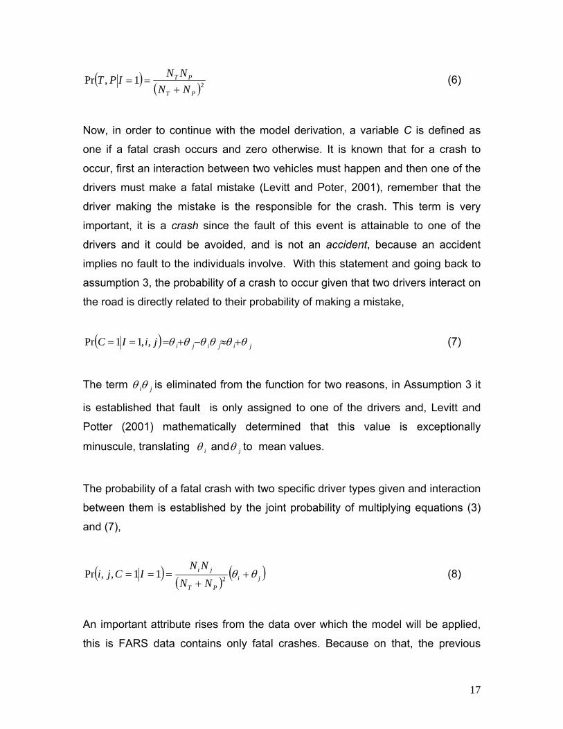
Now, in order to continue with the model derivation, a variable C is defined as

one if a fatal crash occurs and zero otherwise. It is known that for a crash to

occur, first an interaction between two vehicles must happen and then one of the

drivers must make a fatal mistake (Levitt and Poter, 2001), remember that the

driver making the mistake is the responsible for the crash. This term is very

important, it is a crash since the fault of this event is attainable to one of the

drivers and it could be avoided, and is not an accident, because an accident

implies no fault to the individuals involve. With this statement and going back to

assumption 3, the probability of a crash to occur given that two drivers interact on

the road is directly related to their probability of making a mistake,

( ) jijijijiIC θθθθθθ +≈−+=== ,,11Pr (7)

The term jiθθ is eliminated from the function for two reasons, in Assumption 3 it

is established that fault is only assigned to one of the drivers and, Levitt and

Potter (2001) mathematically determined that this value is exceptionally

minuscule, translating iθ and jθ to mean values.

The probability of a fatal crash with two specific driver types given and interaction

between them is established by the joint probability of multiplying equations (3)

and (7),

( )( )

( )jiPT

ji

NNNN

ICji θθ ++

=== 211,,Pr (8)

An important attribute rises from the data over which the model will be applied,

this is FARS data contains only fatal crashes. Because on that, the previous

18

equation has to be altered to read “given a fatal crash” instead of “given an

interaction,”

( ) ( )( )11Pr

11,,Pr1,Pr

====

==IC

ICjiCji

( ) ( )( ) ( ) ( )[ ]222

1,PrPPPTPTTT

jiji

NNNNNN

Cjiθθθθ

θθ+++

+== (9)

The previous equation in terms of SUV/SUV, SUV/P and P/P driver

configurations is,

( ) ( )( ) ( ) ( )[ ]22

2

1,PrPPPTPTTT

TTTT NNNN

NCTjTiPθθθθ

θ+++

===== (10)

( ) ( )( ) ( ) ( )[ ]221,Pr

PPPTPTTT

PTPTTP NNNN

NNCPjTiPθθθθ

θθ+++

+===== (11)

( ) ( )( ) ( ) ( )[ ]22

2

1,PrPPPTPTTT

PPPP NNNN

NCPjPiPθθθθ

θ+++

===== (12)

One issue here is that there are four unknown parameters Pθ , Tθ , PN , and TN ,

and only three equations are available to solve this system (11-13). This was

solved by Levitt and Potter using ratios for the parameters instead of the

individual ones,

P

T

θθθ = (13)

19

P

T

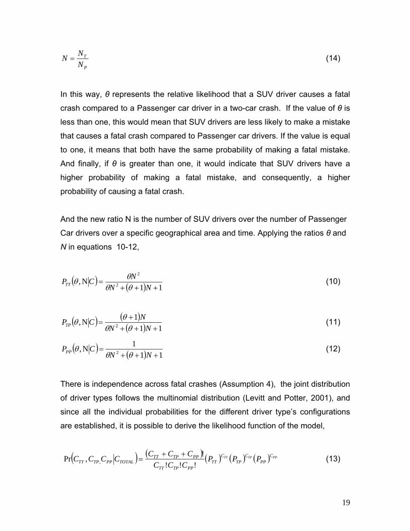
NNN = (14)

In this way, θ represents the relative likelihood that a SUV driver causes a fatal

crash compared to a Passenger car driver in a two-car crash. If the value of θ is

less than one, this would mean that SUV drivers are less likely to make a mistake

that causes a fatal crash compared to Passenger car drivers. If the value is equal

to one, it means that both have the same probability of making a fatal mistake.

And finally, if θ is greater than one, it would indicate that SUV drivers have a

higher probability of making a fatal mistake, and consequently, a higher

probability of causing a fatal crash.

And the new ratio N is the number of SUV drivers over the number of Passenger

Car drivers over a specific geographical area and time. Applying the ratios θ and

N in equations 10-12,

( ) ( ) 11N, 2

2

+++=

NNNCPTT θθθθ (10)

( ) ( )( ) 11

1N, 2 ++++

=NN

NCPTP θθθθ (11)

( ) ( ) 111N, 2 +++

=NN

CPPP θθθ (12)

There is independence across fatal crashes (Assumption 4), the joint distribution

of driver types follows the multinomial distribution (Levitt and Potter, 2001), and

since all the individual probabilities for the different driver type’s configurations

are established, it is possible to derive the likelihood function of the model,

( ) ( ) ( ) ( ) ( ) PPTPTT CPP

CTP

CTT

PPTPTT

PPTPTTTOTALPPTPTT PPP

CCCCCCCCCC

!!!!,Pr ,

++= (13)

20

In a practical manner, it is obvious that the maximum likelihood estimate of

crashes involving two specific types of drivers is just the fraction of those driver

type configurations with respect to all the fatal crashes, which means,

TOTAL

TTTT C

CP =ˆ (14)

TOTAL

TPTP C

CP =ˆ (15)

TOTAL

PPPP C

CP =ˆ (16)

It is desired to determine the relative crash risk of SUV and Passenger Cars

exclusively based on the observed fatal crash distribution, this encourages the

search for a ratio which allows it. By the binomial distribution, it is known that the

squared of the interactions SUV/PC is in fixed proportion to the product of

SUV/SUV and PC/PC (Levitt and Poter, 2001), this is obtained through,

( )( )( )

( ) ( ) ⎟⎟⎠

⎞⎜⎜⎝

⎛+++⎟⎟

⎠

⎞⎜⎜⎝

⎛+++

⎟⎟⎠

⎞⎜⎜⎝

⎛+++

+

=

111

11

111

22

2

2

22

NNNNN

NNN

CCC

PPTT

TP

θθθθθ

θθθ

( ) ( ) ( )[ ] ( ) ( )θ

θθθθ

θθ

θθ

θθ 1212111 22

2

22

2

222

++=++

=+

=+

=+

==N

NN

NPP

PCC

C

PPTT

TP

PPTT

TP (17)

If the previous equation is equaled to a variable named R,

( )PPTT

TP

CCCR

2

≡

21

Then,

θθ 12 ++≡R

θθ 12 =−−R

12 =−− θθθθR

012 =−−− θθθθR

( ) 0122 =−−−− θθ R

( ) 0122 =+−+ θθ R (18)

The solution roots of equation (18) can be found through,

( ) ( ) ( ) ( )2

422

44422

422 222 RRRRRRRR −±−=

−+−±−=

−−±−−=θ (19)

In conclusion, knowing CTT, CTP and CPP in a specific geographical area and

time, R can be computed, N and ultimately θ, which is the value of interest.

The standard error for the maximum likelihood estimation can be determined

based of the Hessian matrix, which is the matrix of second partial derivatives of

the model likelihood function (Appendix A).

⎥⎥⎥⎥

⎦

⎤

⎢⎢⎢⎢

⎣

⎡

∂∂

∂∂∂

∂∂∂

∂∂

=

2

22

2

2

2

PrPr

PrPr

NN

NHessian

θ

θθ (20)

The corresponding variance is,

[ ] 1−−= HessianVar (21)

22

Finally, the standard error can be computed by obtained the squared root of the

diagonal elements of the variance matrix divided by the sample size minus one,

for θ and N.

)1(PrPrPrPr

Pr

22

2

2

2

2

2

2

−⎥⎦

⎤⎢⎣

⎡⎟⎟⎠

⎞⎜⎜⎝

⎛∂∂

∂×

∂∂∂

−⎟⎟⎠

⎞⎜⎜⎝

⎛∂∂

×∂∂

∂∂

−=

TTCNNN

N

θθθ

σθ (22)

)1(PrPrPrPr

Pr

22

2

2

2

2

2

2

−⎥⎦

⎤⎢⎣

⎡⎟⎟⎠

⎞⎜⎜⎝

⎛∂∂

∂×

∂∂∂

−⎟⎟⎠

⎞⎜⎜⎝

⎛∂∂

×∂∂

∂∂

−=

TT

N

CNNN θθθ

θσ (23)

3.4 Scope and limitations of the model

By adapting the Levitt and Potter (2001) model to the particular case of crashes

involving SUVs and Passenger Cars, it can be determined if a different behavior

is developed on the studied driver types through θ. However, this offsetting

behavior cannot be completely separated of preexisting driver characteristics.

For the particular case of SUV drivers, the simple purchase of the vehicle may

demonstrate a pre-existing tendency towards higher risk behavior.

3.5 Data characteristics

The model developed by Levitt and Potter (2001) was developed considering

FARS data characteristics; this project also focuses on this database. The first

step was examining the FARS data at nationwide level, and pulling out only the

records belonging to drivers of two-car crashes.

23

One fundamental assumption of the model is that homogeneity is demanded in

space and time in order to work properly. This means that not only areas with

same characteristics have to been bounded, but also period of times when the

economic and social factors do not affect significantly the driving patterns.

In order to take care of the space homogeneity constraint, the model is applied

independently in six areas,

1) Mid-Atlantic States

2) Mid-West States

3) New England States

4) South States

5) Texas (Two cases)

6) West Coast States

Over these regions, the major Metropolitan Statistical Areas (MSA) were

selected, always trying to built clusters or corridors areas (Appendix B). Since

one of Plaut (2004) findings was that SUV owners have a tendency to live in rural

areas within MSA. In this way a balanced presence of SUVs is warranted.

Besides, it was desirable to create these clusters to get a convenient sample

size. Also, by using MSAs it is more likely to have homogeneity in terms of

preexisting driver risk taking level.

With respect to time homogeneity, it was established that a period of three years

would be an appropriate approach, this also serves to warrant enough crashes

involving two SUV drivers. The periods are 1995-1997, 1996-1998, 1997-1999,

1998-2000, 1999-2001, 2000-2002, 2001-2003, 2002-2004, 2003-2005, and

2004-2006. Some periods are not available for all regions. Those are indicated

subsequently.

24

Finally, there were concerns about what impact alcohol presence would have in

the results. To avoid a confounding effect between driver offsetting behavior and

drinking drivers, only crashes that occurred on Monday, Tuesday, Wednesday,

Thursday and Friday between 6:00 and 17:59 hours were analyzed, since there

is a lower presence of drinking drivers is expected during those times.

Also, it is important to mention that this time restriction allows focusing in a more

homogeneous population in terms of risk taking behavior regardless of the

vehicle body type driven. It is a common belief that there are certain times of the

day the drivers engage in a more reckless driving.

3.6 Selected data

Applying the criteria established in section 3.4, the fatal crashes selected were

those,

1) Were two cars were involved,

2) The two driver records were available and complete,

3) Occurred between 6:00 and 17:59 hours,

4) Took place Monday, Tuesday, Wednesday, Thursday or Friday, and

5) Happened on the states and counties specified in Appendix B.

The following tables are summaries of the fatal two-crashes that fulfilled those

selection criteria,

25

Table 3.6.1 Mid-Atlantic Region Two-Car Fatal Crashes

Fatal Crashes for Driver Type Configuration Period P/P P/SUV SUV/SUV Total

1995-1997 344 120 5 469 1996-1998 335 135 4 474 1997-1999 327 128 6 461 1998-2000 306 132 4 442 1999-2001 280 125 6 411 2000-2002 265 140 4 409 2001-2003 260 144 7 411 2002-2004 264 162 6 432 2003-2005 247 166 8 421 2004-2006 212 166 13 391

Table 3.6.2 Mid-West Region Two-Car Fatal Crashes


1995-1997 348 97 0 445 1996-1998 328 85 0 413 1997-1999 304 78 0 382 1998-2000 289 88 2 379 1999-2001 291 102 7 400 2000-2002 281 129 7 417 2001-2003 280 150 9 439 2002-2004 233 157 6 396 2003-2005 225 151 12 388 2004-2006 200 134 11 345

Table 3.6.3 New England Region Two-Car Fatal Crashes


1995-1997 94 27 1 122 1996-1998 85 30 1 116 1997-1999 76 38 3 117 1998-2000 65 37 4 106 1999-2001 58 36 3 97 2000-2002 62 31 1 94 2001-2003 68 30 1 99 2002-2004 66 32 2 100 2003-2005 62 42 2 106 2004-2006 59 50 2 111

26

Table 3.6.4 South Region Two-Car Fatal Crashes


1995-1997 357 77 0 434 1996-1998 358 102 2 462 1997-1999 342 120 5 467 1998-2000 312 139 6 457 1999-2001 274 139 6 419 2000-2002 249 140 8 397 2001-2003 232 129 11 372 2002-2004 223 135 12 370 2003-2005 232 159 15 406 2004-2006 221 184 20 425

Table 3.6.5 Texas Two-Car Fatal Crashes (Case 1. Table)


1995-1997 101 35 1 137 1996-1998 102 39 1 142 1997-1999 101 39 1 141 1998-2000 92 41 1 134 1999-2001 84 42 2 128 2000-2002 74 47 1 122 2001-2003 62 62 2 126 2002-2004 61 62 3 126 2003-2005 57 62 6 125 2004-2006 55 55 8 118

Table 3.6.6 Texas Two-Car Fatal Crashes (Case 2. Table)


1995-1997 117 40 1 158 1996-1998 118 45 1 164 1997-1999 116 43 1 160 1998-2000 104 49 2 155 1999-2001 96 51 3 150 2000-2002 91 60 2 153 2001-2003 81 75 4 160 2002-2004 84 71 5 160 2003-2005 75 71 8 154 2004-2006 71 61 8 140

27

Table 3.6.7 West Coast Region Two-Car Fatal Crashes


1995-1997 345 128 1 474 1996-1998 324 131 3 458 1997-1999 319 135 5 459 1998-2000 287 154 9 450 1999-2001 281 183 12 476 2000-2002 280 190 16 486 2001-2003 309 191 18 518 2002-2004 293 181 21 495 2003-2005 274 181 19 474 2004-2006 238 185 18 441

28

4. RESULTS

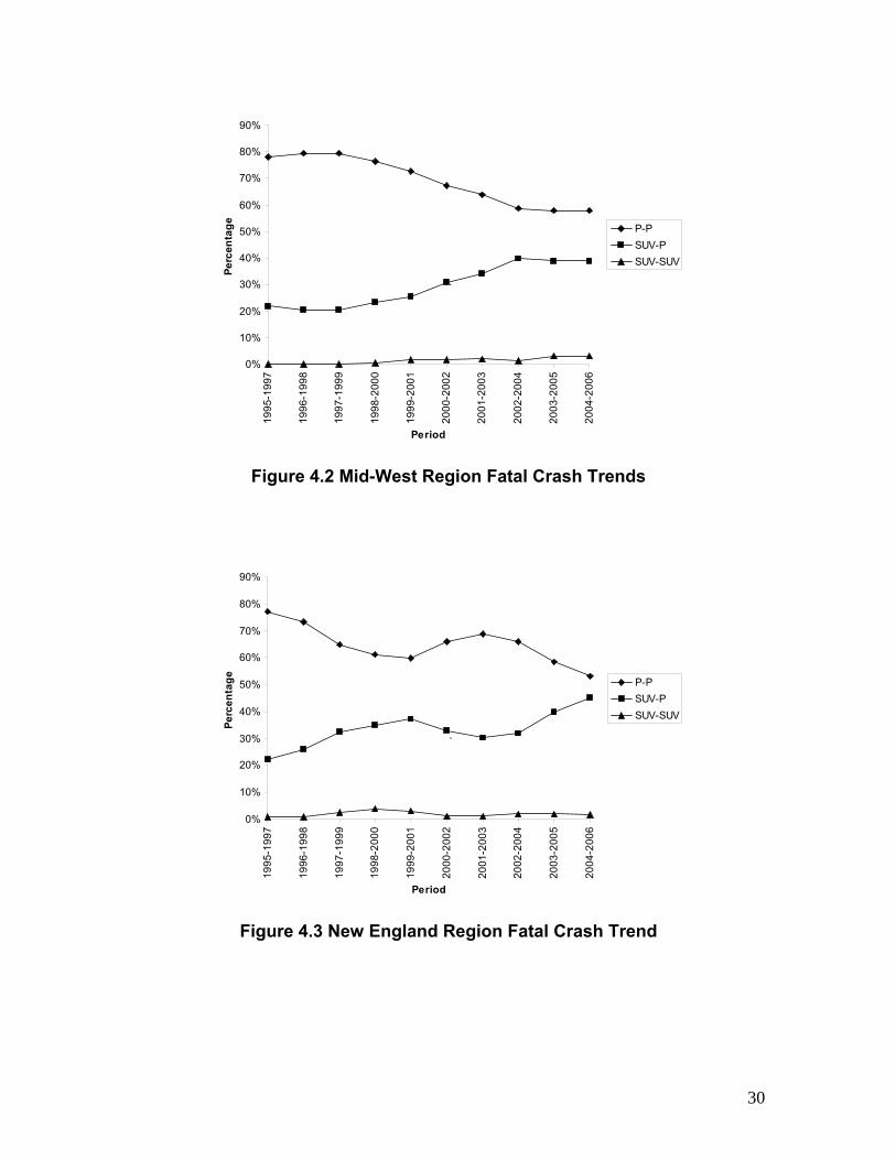
In general terms, when analyzing the New England States (Figure 4.3) and West

Coast Region (Figure 4.7), it was found that the number of fatal crashes involving

P/P drivers have been decreasing, P/SUV drivers has been increasing and,

SUV/SUV has remained relatively stable over the last ten years, but for 2000-

2002 and 2001-2003 the trend was the opposite for P/P and P/SUV.

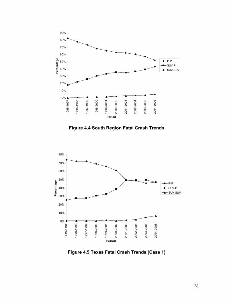
For the Mid-Atlantic (Figure 4.1) and South regions (Figure 4.4), there is a clear

pattern of decreasing numbers of P/P, and an increase of SUV/P fatal crashes;

also fatal crashes involving two SUV drivers remain at a constant and low level.

For the Mid-West region (Figure 4.3), an important development is found: , there

is a decreasing trend of P/P and an increasing trend in P/SUV, while SUV/SUV

fatal crashes stay at a flat rate. However, it seems that an equilibrium is reached

after 2002-2004, since the two curves are almost parallel to each other.

An a particular trend happened in Texas Case 1 (Figure 4.5) where the

decreasing trend of P/P fatal crashes is overtaken by a significant increase in

SUV/P fatal crashes and at the intervals 2001-2003 to 2003-2005 there are

more SUV/P than P/P fatal crashes.

In conclusion, for all the regions studied, during the last 11 years there has been

a decreasing trend in the number of two-car crashes involving two passenger car

drivers. The opposite has happened to the P/SUV fatal crashes, and for

SUV/SUV fatal crashes there has not been a change in the crash rates.

By itself, the previous analysis is week, but it raises several interesting questions,

1) Are the decreasing patterns in P/P fatal crashes attainable to safer

passenger cars design in later years?

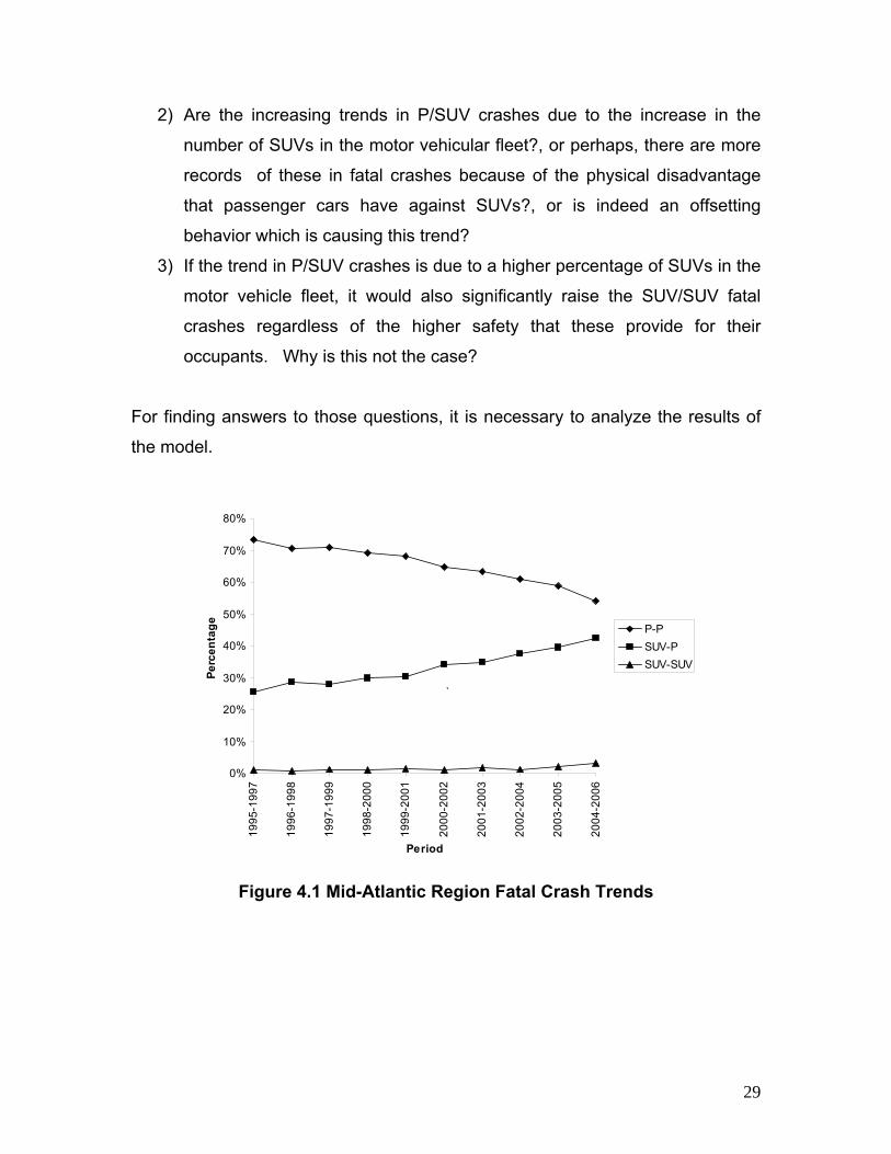
29

2) Are the increasing trends in P/SUV crashes due to the increase in the

number of SUVs in the motor vehicular fleet?, or perhaps, there are more

records of these in fatal crashes because of the physical disadvantage

that passenger cars have against SUVs?, or is indeed an offsetting

behavior which is causing this trend?

3) If the trend in P/SUV crashes is due to a higher percentage of SUVs in the

motor vehicle fleet, it would also significantly raise the SUV/SUV fatal

crashes regardless of the higher safety that these provide for their

occupants. Why is this not the case?

For finding answers to those questions, it is necessary to analyze the results of

the model.

0%

10%

20%

30%

40%

50%

60%

70%

80%

1995

-199

7

1996

-199

8

1997

-199

9

1998

-200

0

1999

-200

1

2000

-200

2

2001

-200

3

2002

-200

4

2003

-200

5

2004

-200

6

Period

Perc

enta

ge P-PSUV-PSUV-SUV

`

Figure 4.1 Mid-Atlantic Region Fatal Crash Trends

30

0%

10%

20%

30%

40%

50%

60%

70%

80%

90%

1995

-199

7

1996

-199

8

1997

-199

9

1998

-200

0

1999

-200

1

2000

-200

2

2001

-200

3

2002

-200

4

2003

-200

5

2004

-200

6

Period

Perc

enta

ge P-PSUV-PSUV-SUV

`

Figure 4.2 Mid-West Region Fatal Crash Trends

0%

10%

20%

30%

40%

50%

60%

70%

80%

90%

1995

-199

7

1996

-199

8

1997

-199

9

1998

-200

0

1999

-200

1

2000

-200

2

2001

-200

3

2002

-200

4

2003

-200

5

2004

-200

6

Period

Perc

enta

ge P-PSUV-PSUV-SUV

`

Figure 4.3 New England Region Fatal Crash Trend

31

0%

10%

20%

30%

40%

50%

60%

70%

80%

90%

1995

-199

7

1996

-199

8

1997

-199

9

1998

-200

0

1999

-200

1

2000

-200

2

2001

-200

3

2002

-200

4

2003

-200

5

2004

-200

6

Period

Perc

enta

ge P-PSUV-PSUV-SUV

`

Figure 4.4 South Region Fatal Crash Trends

0%

10%

20%

30%

40%

50%

60%

70%

80%

1995

-199

7

1996

-199

8

1997

-199

9

1998

-200

0

1999

-200

1

2000

-200

2

2001

-200

3

2002

-200

4

2003

-200

5

2004

-200

6

Period

Perc

enta

ge P-PSUV-PSUV-SUV

`

Figure 4.5 Texas Fatal Crash Trends (Case 1)

32

0%

10%

20%

30%

40%

50%

60%

70%

80%

1995

-199

7

1996

-199

8

1997

-199

9

1998

-200

0

1999

-200

1

2000

-200

2

2001

-200

3

2002

-200

4

2003

-200

5

2004

-200

6

Period

Perc

enta

ge P-PSUV-PSUV-SUV

`

Figure 4.6 Texas Fatal Crash Trends (Case 2)

0%

10%

20%

30%

40%

50%

60%

70%

80%

1995

-199

7

1996

-199

8

1997

-199

9

1998

-200

0

1999

-200

1

2000

-200

2

2001

-200

3

2002

-200

4

2003

-200

5

2004

-200

6

Period

Perc

enta

ge P-PSUV-PSUV-SUV

`

Figure 4.7 West Coast Region Fatal Crash Trends

33

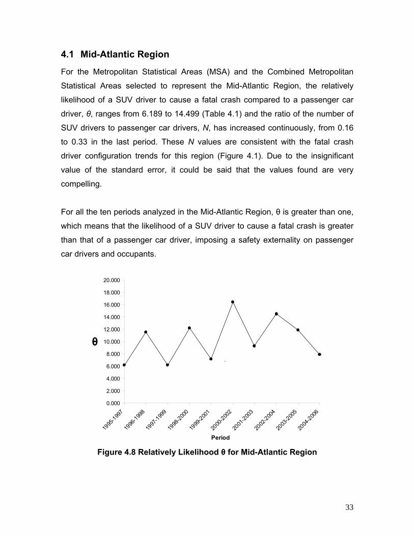
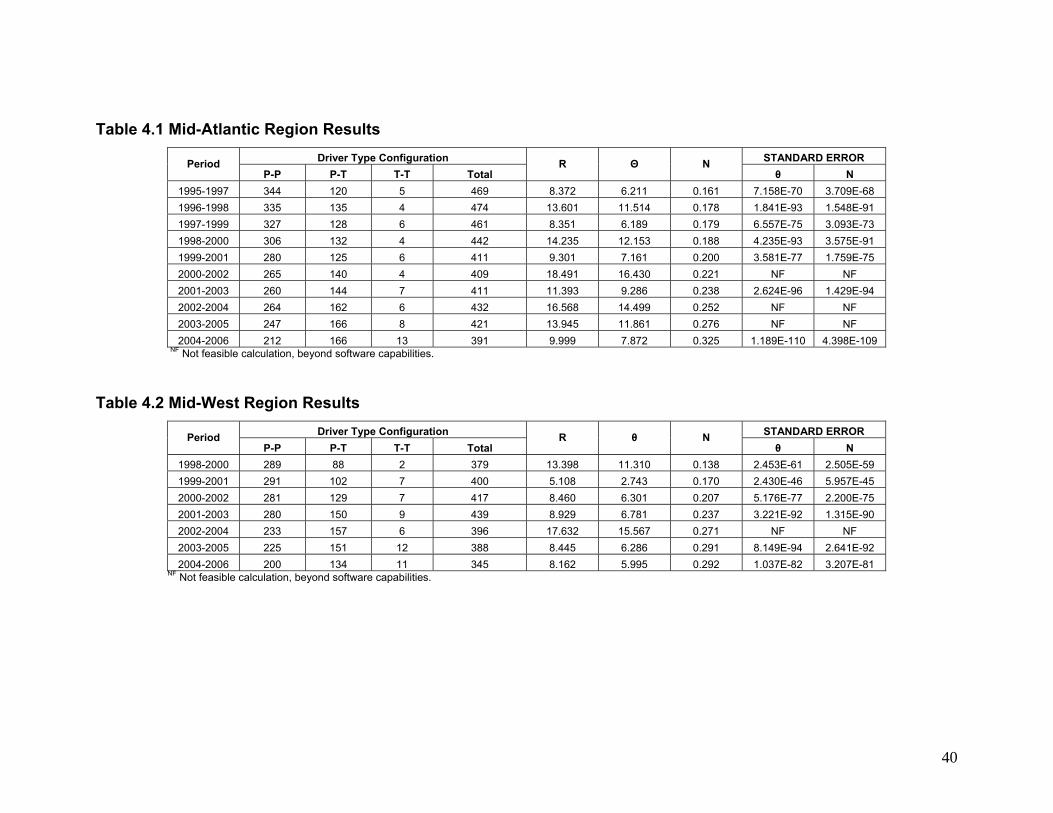
4.1 Mid-Atlantic Region

For the Metropolitan Statistical Areas (MSA) and the Combined Metropolitan

Statistical Areas selected to represent the Mid-Atlantic Region, the relatively

likelihood of a SUV driver to cause a fatal crash compared to a passenger car

driver, θ, ranges from 6.189 to 14.499 (Table 4.1) and the ratio of the number of

SUV drivers to passenger car drivers, N, has increased continuously, from 0.16

to 0.33 in the last period. These N values are consistent with the fatal crash

driver configuration trends for this region (Figure 4.1). Due to the insignificant

value of the standard error, it could be said that the values found are very

compelling.

For all the ten periods analyzed in the Mid-Atlantic Region, θ is greater than one,

which means that the likelihood of a SUV driver to cause a fatal crash is greater

than that of a passenger car driver, imposing a safety externality on passenger

car drivers and occupants.

0.000

2.000

4.000

6.000

8.000

10.000

12.000

14.000

16.000

18.000

20.000

1995

-1997

1996

-1998

1997

-1999

1998

-2000

1999

-2001

2000

-2002

2001

-2003

2002

-2004

2003

-2005

2004

-2006

Period

θ `

Figure 4.8 Relatively Likelihood θ for Mid-Atlantic Region

34

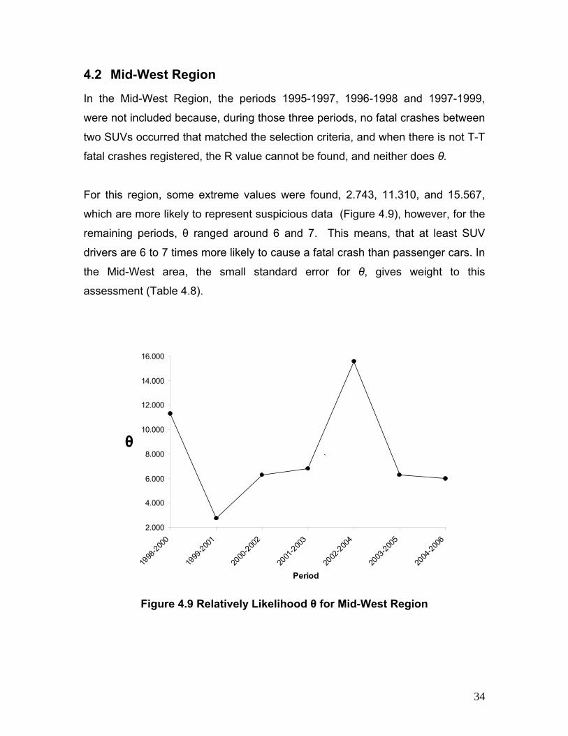
4.2 Mid-West Region

In the Mid-West Region, the periods 1995-1997, 1996-1998 and 1997-1999,

were not included because, during those three periods, no fatal crashes between

two SUVs occurred that matched the selection criteria, and when there is not T-T

fatal crashes registered, the R value cannot be found, and neither does θ.

For this region, some extreme values were found, 2.743, 11.310, and 15.567,

which are more likely to represent suspicious data (Figure 4.9), however, for the

remaining periods, θ ranged around 6 and 7. This means, that at least SUV

drivers are 6 to 7 times more likely to cause a fatal crash than passenger cars. In

the Mid-West area, the small standard error for θ, gives weight to this

assessment (Table 4.8).

2.000

4.000

6.000

8.000

10.000

12.000

14.000

16.000

1998

-2000

1999

-2001

2000

-2002

2001

-2003

2002

-2004

2003

-2005

2004

-2006

Period

θ `

Figure 4.9 Relatively Likelihood θ for Mid-West Region

35

4.3 New England Region

In the New England Region, the sample taken might be relatively small in

comparison to the other regions. A clear proof of this is that the total number of

fatal crashes was around 100, and for the other regions it was approximately four

times that. Despite this, it was possible to ensure homogeneity on the area since

there was enough data to compute all the parameters and mainly, the standard

error was extremely small. In general, θ ranged from 2.892 to 19.134 (Table 4.3),

but the last value is more likely to represent suspicious data and in general the

probability of a SUV driver to cause a fatal crash against a Passenger Car driver

is between 2 to 8 (Figure 4.10).

0

2

4

6

8

10

12

14

16

18

20

1995

-1997

1996

-1998

1997

-1999

1998

-2000

1999

-2001

2000

-2002

2001

-2003

2002

-2004

2003

-2005

2004

-2006

Period

θ `

Figure 4.10 Relatively Likelihood θ for New England Region

36

4.4 South Region

The South Region represents an area, where, at first sight, it appears that the

risk that SUV drivers pose on Passenger Car drivers is decreasing, but this is a

erroneous interpretation induced in the results because of some suspicious data

that may represents special circumstances for those periods (Figure 4.11).

Mainly, θ ranges between 4 and 8, and since 2000-2002, θ has been increasing.

The results suggest that, at least in the past eleven years, an SUV driver has

been 4.28 times more likely to cause a fatal crash than a passenger car driver.

0.000

2.000

4.000

6.000

8.000

10.000

12.000

14.000

1995-199

7

1996-199

8

1997-199

9

1998-200

0

1999-200

1

2000-200

2

2001-200

3

2002

-2004

2003

-2005

Period

θ `

Figure 4.11 Relatively Likelihood θ for South Region

37

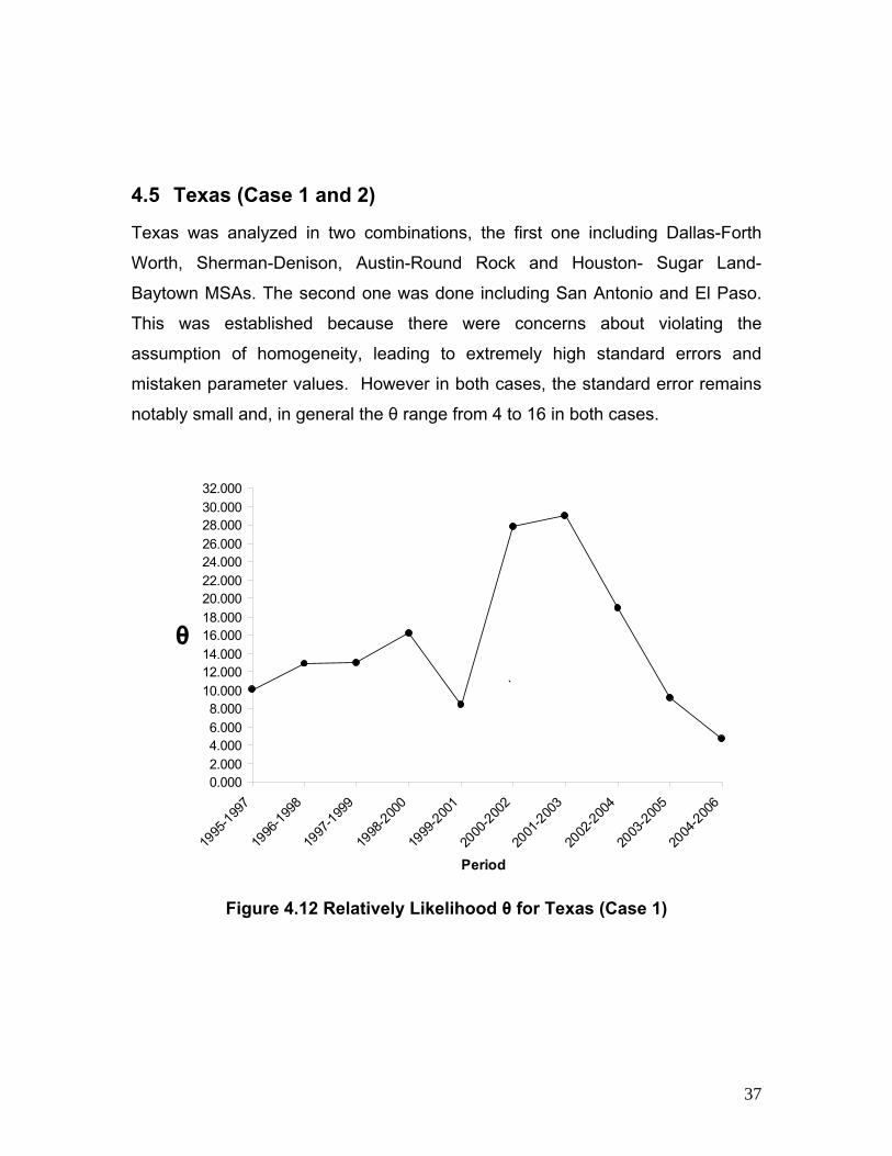
4.5 Texas (Case 1 and 2)

Texas was analyzed in two combinations, the first one including Dallas-Forth

Worth, Sherman-Denison, Austin-Round Rock and Houston- Sugar Land-

Baytown MSAs. The second one was done including San Antonio and El Paso.

This was established because there were concerns about violating the

assumption of homogeneity, leading to extremely high standard errors and

mistaken parameter values. However in both cases, the standard error remains

notably small and, in general the θ range from 4 to 16 in both cases.

0.0002.0004.0006.0008.000

10.00012.00014.00016.00018.00020.00022.00024.00026.00028.00030.00032.000

1995

-1997

1996

-1998

1997

-1999

1998

-2000

1999

-2001

2000

-2002

2001

-2003

2002

-2004

2003

-2005

2004

-2006

Period

θ

`

Figure 4.12 Relatively Likelihood θ for Texas (Case 1)

38

0.000

2.000

4.000

6.000

8.000

10.000

12.000

14.000

16.000

18.000

20.000

1995

-1997

1996

-1998

1997

-1999

1998

-2000

1999

-2001

2000

-2002

2001

-2003

2002

-2004

2003

-2005

2004

-2006

Period

θ

`

Figure 4.13 Relatively Likelihood θ for Texas (Case 2)

39

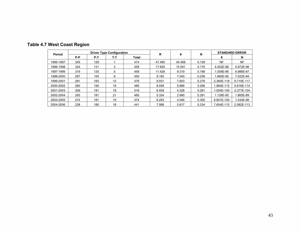
4.6 West Coast Region

The West Coast Region has some suspicious data around 45.468; this is

because from 1995-1997 only one fatal crash involving two SUVs complies with

the selection criteria (Table 4.7). In general, the relative probability θ, ranges

from 3 to 15 for those three-year periods, and it can be appreciated a trend for θ

were its value is stabilizing.

Figure 4.14 Relatively Likelihood θ for West Coast Region

0.000

5.000

10.000

15.000

20.000

25.000

30.000

35.000

40.000

45.000

50.000

1995

-1997

1996

-1998

1997

-1999

1998

-2000

1999

-2001

2000

-2002

2001

-2003

2002

-2004

2003

-2005

2004

-2006

Period

θ

`

40

Table 4.1 Mid-Atlantic Region Results Driver Type Configuration STANDARD ERROR Period

P-P P-T T-T Total R Θ N

θ N 1995-1997 344 120 5 469 8.372 6.211 0.161 7.158E-70 3.709E-68 1996-1998 335 135 4 474 13.601 11.514 0.178 1.841E-93 1.548E-91 1997-1999 327 128 6 461 8.351 6.189 0.179 6.557E-75 3.093E-73 1998-2000 306 132 4 442 14.235 12.153 0.188 4.235E-93 3.575E-91 1999-2001 280 125 6 411 9.301 7.161 0.200 3.581E-77 1.759E-75 2000-2002 265 140 4 409 18.491 16.430 0.221 NF NF 2001-2003 260 144 7 411 11.393 9.286 0.238 2.624E-96 1.429E-94 2002-2004 264 162 6 432 16.568 14.499 0.252 NF NF 2003-2005 247 166 8 421 13.945 11.861 0.276 NF NF 2004-2006 212 166 13 391 9.999 7.872 0.325 1.189E-110 4.398E-109

NF Not feasible calculation, beyond software capabilities.

Table 4.2 Mid-West Region Results Driver Type Configuration STANDARD ERROR Period

P-P P-T T-T Total R θ N

θ N 1998-2000 289 88 2 379 13.398 11.310 0.138 2.453E-61 2.505E-59 1999-2001 291 102 7 400 5.108 2.743 0.170 2.430E-46 5.957E-45 2000-2002 281 129 7 417 8.460 6.301 0.207 5.176E-77 2.200E-75 2001-2003 280 150 9 439 8.929 6.781 0.237 3.221E-92 1.315E-90 2002-2004 233 157 6 396 17.632 15.567 0.271 NF NF 2003-2005 225 151 12 388 8.445 6.286 0.291 8.149E-94 2.641E-92 2004-2006 200 134 11 345 8.162 5.995 0.292 1.037E-82 3.207E-81

NF Not feasible calculation, beyond software capabilities.

41

Table 4.3 New England Region Results Driver Type Configuration STANDARD ERROR Period


θ N 1995-1997 94 27 1 122 7.755 5.576 1.349E-01 9.292E-18 5.079E-16 1996-1998 85 30 1 116 10.588 8.470 1.600E-01 6.884E-22 4.735E-20 1997-1999 76 38 3 117 6.333 4.089 2.316E-01 1.438E-22 3.76E-21 1998-2000 65 37 4 106 5.265 2.923 2.695E-01 2.136E-20 3.646E-19 1999-2001 58 36 3 97 7.448 5.258 2.763E-01 1.245E-23 3.538E-22 2000-2002 62 31 1 94 15.500 13.426 2.129E-01 1.580E-25 1.326E-23 2001-2003 68 30 1 99 13.235 11.146 1.928E-01 1.215E-23 9.242E-22 2002-2004 66 32 2 100 7.758 5.578 2.195E-01 4.176E-21 1.507E-19 2003-2005 62 42 2 106 14.226 12.143 2.771E-01 4.075E-33 2.551E-31 2004-2006 59 50 2 111 21.186 19.134 3.214E-01 2.817E-43 2.487E-41

Table 4.4 South Region Driver Type Configuration STANDARD ERROR Period


θ N 1996-1998 358 102 2 462 14.531 12.450 0.130 4.277E-72 5.051E-70 1997-1999 342 120 5 467 8.421 6.261 0.162 4.553E-70 2.366E-68 1998-2000 312 139 6 457 10.321 8.199 0.198 1.643E-88 9.219E-87 1999-2001 274 139 6 419 11.752 9.649 0.220 2.744E-93 1.648E-91 2000-2002 249 140 8 397 9.839 7.710 0.245 1.164E-89 5.213E-88 2001-2003 232 129 11 372 6.521 4.288 0.255 4.386E-71 1.113E-69 2002-2004 223 135 12 370 6.811 4.593 0.274 1.118E-76 2.847E-75 2003-2005 232 159 15 406 7.265 5.067 0.303 6.161E-94 1.584E-92 2004-2006 221 184 20 425 7.660 5.477 0.358 3.078E-114 7.528E-113 1996-1998 358 102 2 462 14.531 12.450 0.130 4.277E-72 5.051E-70

42

Table 4.5 Texas (Case 1) Driver Type Configuration STANDARD ERROR Period



Table 4.6 Texas (Case 2) Driver Type Configuration STANDARD ERROR Period



43

Table 4.7 West Coast Region Driver Type Configuration STANDARD ERROR Period


θ N 1995-1997 345 128 1 474 47.490 45.468 0.159 NF NF 1996-1998 324 131 3 458 17.655 15.591 0.176 4.402E-98 4.972E-96 1997-1999 319 135 5 459 11.426 9.319 0.188 1.059E-88 6.986E-87 1998-2000 287 154 9 450 9.182 7.040 0.236 1.660E-95 7.022E-94 1999-2001 281 183 12 476 9.931 7.803 0.278 2.360E-118 9.710E-117 2000-2002 280 190 16 486 8.058 5.888 0.296 1.864E-115 5.616E-114 2001-2003 309 191 18 518 6.559 4.328 0.281 1.004E-105 2.377E-104 2002-2004 293 181 21 495 5.324 2.990 0.291 1.128E-90 1.865E-89 2003-2005 274 181 19 474 6.293 4.046 0.300 6.801E-100 1.434E-98 2004-2006 238 185 18 441 7.989 5.817 0.334 7.654E-115 2.082E-113

44

5. CONCLUSIONS

During the past ten years, there has been a substantial increase of SUVs sales.

This raised concerns about road vehicular incompatibility and offsetting driver

behavior. Several studies had addressed the vehicular incompatibility, one of

them developed by Gabler and Hollowell (1998) by finding a measurement of

Design Vehicle Aggressivity, ranked SUVs as the third more aggressive motor

vehicle type.

This project focused on determining if a safety externality was posed on

passenger cars by SUV drivers. The basic hypothesis was that SUVs have

certain safety characteristics that, through the Peltzman Effect, lead their drivers

to take compensatory risks that impose additional risk to passenger cars. The

SUV safety characteristics include higher mass, four-wheel drive, higher seating

position, and stiffer suspensions. This perception situates the driver in a unique

place where he or she can deliberately trade some of this safety for a more

convenient driving experience, like shorter driving time to reach a destination,

driving at higher speeds, or even doing right turn on red (RTOR) without a

complete stop more often. This risk-taking behavior is a Peltzman Effect, and this

riskier driving does not affect the SUV driver, it affects the passenger car drivers

and occupants, since they are paying the externality for this offsetting behavior.

Also, due to the physical disadvantage that a passenger car has against an SUV,

is more likely that the fatalities are located in the passenger car as the

Aggressivity Metric of Gabler and Hollowell.

It is possible to know how many SUVs are registered, but it is almost unfeasible

to determine how many SUVs and Passenger cars are in a given time or period

on the roads. This complicated the scenario to determine if SUVs are liable for

causing more fatal crashes. However, this problem was solved previously by

Levitt and Poter (2001) when analyzed how dangerous drinking drivers are.

Since this was an acceptable method for the current problem, it was applied.

45

First, a way to comply with the assumptions was established, the main concern

was the assumption of homogeneity (Assumption 3), since issues as a small

sample size, or a large standard error could develop from here. The nationwide

data was disaggregated into regions (Mid-Atlantic, Mid-West, New England,

Texas, South and West Coast) and only major MSAs and CMSAs were selected,

trying to create a cluster or corridor. Also, time restrictions were posed in the

selection criteria (Fatal crashes that happened only Monday through Friday

between 6am-5:59pm), to control for drinking drivers and to ensure the same

level of preexisting risk taking behavior. Once the data was selected, the method

was applied.

5.1 Findings

The general trend in the fatal crashes registered since 1995-2006 is a decrease

of those between two passenger cars; a significant increase of fatal crashes

involving an SUV and a passenger car; and those involving two SUVs remains

almost at the same level. It could be thought that this increase in SUV and

passenger car is due to the higher number of SUVs on the road, which increases

the probability of a crash with a vehicle of this type. However, if this were true,

the number or fatal crashes involving two SUVs would also rise, although not at

the same rate as in SUV and passenger car, but it would not show a flat level

over time, as the current one. Therefore, it can be concluded that SUVs pose a

higher danger on passenger cars occupants than on other SUVs occupants.

In all the regions studied across all the periods analyzed, it was consistently

found that SUVs are more likely to cause a fatal crash than a passenger car, at

least 2.7 times. The values found in this project are similar to the results of Gayer

(2007) that determined that light trucks are between 2.63 and 4 times more likely

to crash. The standard errors for all these estimates are insignificant, and

because of that the previous statement has value. This higher probability to

46

cause a fatal crash may be attainable to a Peltzman effect or offsetting behavior

by the SUV driver, and supports the initial idea of the externality posed on

passenger cars.

5.2 Future Research

SUVs have been studied from very different approaches in order to ensure safety

for the owners, users, and the non-users. However, it could be desirable to study

driving behavior patrons from a quantitative point, such as measuring the speeds

that a subject drives on the same section of road, using an SUV and a passenger

car.

Also, this current project could be taken a step forward by also controlling and

analyzing for driving record patrons, like number or DUIs of the driver, speeding

tickets and other related traffic infractions, that may confirm the offsetting

behavior. Another approach that could be interesting to analyze, is to carry the

study at the state level perhaps by disaggregating the nationwide data by states

and choose only one year, to check for homogeneity and monitoring the standard

error for these subsets.

And finally, the value of this externality that SUVs pose on passenger cars should

be quantified and determine if a government measure should be applied.

47

REFERENCE LIST

Abdelwahab, H.; and Abdel-Aty, M; “Investigating the Effect of Light Truck

Vehicle Percentages on Head-On Fatal Traffic Crashes”, Journal of

Transportation Engineering, Vol. 130, No. 4, pp. 429-437.

American National Standard Institute. “Manual on Classification of Motor Vehicle

Traffic Accidents”, National Safety Council. 6th ed.,

http://www.nhtsa.dot.gov/people/perform/trafrecords/crash/pdf/d16.pdf,

Accessed February 22, 2008.

Bradsher, K. (2002) “High And Mighty: SUVs – The World’s Most Dangerous

Vehicle and How They Got That Way?”, Public Affairs.

Bureau of Transportation Statistics. “Table 1-20: Period Sales, Market Shares,

and Sales-Weighted Fuel Economies of New Domestic and Imported Light

Trucks (Thousands of vehicles)”

www.bts.gov/publications/national_transportation_statistics/csv/table_01_

20.csv, Accessed February 19, 2008.

Choo, S.; and Mokhtarian, P. L. (2004) “The role of attitude and lifestyle in

influencing vehicles type choice”, Transportation Research Part A: Policy

and Practice, Vol. 38, No. 3, pp. 201-222.

Energy Information Administration. “Chapter 2. Vehicle Characteristics”,

http://www.eia.doe.gov/emeu/rtecs/chapter2.html. Accessed March 22,

2008.

Fatality Analysis Reporting System. “National Statistics”. http://www-

fars.nhtsa.dot.gov/Main/index.aspx. Accessed February 22, 2008.

48

Gabler, H.C.; and Hollowell, W.T. (1998) “Aggressivity of light trucks and Vans in

Traffic Crashes”, SAE Special Publications, Vol. 1333, Airbag Technology,

pp 125-133.

Gayer, T. (2004) “The Fatality Risks of Sport-Utility Vehicles, Vans, and Pickups

Relative to Cars”, The Journal of Risk and Uncertainty, Vol. 28, No. 2, pp.

103-133

Khattak, A.J.; and Fan, Y. (2008) “What Exacerbates Injury and Harm in Car-

SUV Collinsions?” Journal of Transportation Engineering, Vol. 134, No.2,

pp. 93-104

Khattak, A. J.; and Rocha, M. (2003) “Are SUVs ‘Supremely Unsafe Vehicles’?

Analysis of Rollovers and Injuries with Sport Utility Vehicles”,

Transportation Research Record, No. 1840, pp. 167-177

Levitt, S.D.; and Porter, J. (2001) “How Dangerous Are Drinking Drivers?”,

Journal of Political Economy, Vol. 109, No. 6, pp. 1198-1237

Levitt, S.D.: Porter, J. (2001) “Sample Selection in the estimation of air bag and

seat belt effectiveness”, The Review of Economics and Statistics, Vol.

83, Num. 4, pp. 603-615.

Merrian-Webster Online Dictionary. “Sport-Utility Vehicle”. http://www.merriam-

webster.com/dictionary/sport-utility+vehicle, Accessed March 19, 2008.

National Center for Health Statistics. “Deaths/Mortality”.

http://www.cdc.gov/nchs/fastats/deaths.htm. Accessed February 22, 2008.

49

National Highway Traffic Safety Administration. National Center for Statistics and

Analysis. “Fatal Crash Data Overview (Brochure)” http://www-

nrd.nhtsa.dot.gov/Pubs/FARSBROCHURE.PDF. Accessed March 21,

2008.

Peltzman, S. (1975) “The Effects of Automobile Safety Regulation”, The Journal

of Political Economy, Vol. 83, No. 4, pp. 677-726

Peterson, S.; Hoffer, G.; and Millner, E. (1995) “Are drivers of air-bag-equipped

cars more aggressive? A test of the offsetting behavior hypothesis”,

Journal of Law and Economics, Vol. 38, No. 2, pp. 251-264.

Plaut, P.O. (2004) “The uses and users of SUVs and light trucks in commuting”,

Transportation Research Part D: Transport and Environment, Vol. 9, No.

3, pp. 175-183

Poitras, M. and Sutter, D. (2002) “Policy Ineffectiveness or Offsetting Behavior?

An Analysis of Vehicle Safety Inspections”, Southern Economic Journal,

Vol. 68, No. 4, pp. 922-934

Robertson, L. (1977) “A Critical Analysis of Peltzman’s ‘The Effects of

Automobile Safety Regulation’ ”, The Journal of Economic Issues, Vol.11,

No. 3, pp. 587-600

Sen, A. (2001) “An Empirical Test of the Offset Hypothesis”, Journal of Law and

Economics, Vol. 44, No. 2. pp. 481-510.

Sobel, R.S; and Nesbit, T.M. (2007) “Automobile Safety Regulation and the

Incentive to Drive Recklessly: Evidence from NASCAR”, Southern

Economic Journal, Vol. 74, No. 1, pp.71-84.

50

Traynor, T.L. (1993) “The Peltzman Hypothesis Revisited: An Isolated Evaluation

of Offsetting Driver Behavior”, Journal of Risk and Uncertainty, Vol. 7, No.

7, pp. 237-247.

Ulfarsson, G.F.; and Mannering, F. (2004) “Differences in male and female injury

severities in sport-utility vehicle, minivan, pickup and passenger car

accidents”, Accident Analysis and Prevention, Vol. 36, No. 2, pp. 135-147.

U.S. Department of Transportation. Office of the Historian. “The United States

Department of Transportation: A Brief History”

http://dotlibrary.dot.gov/Historian/history.htm. Accessed April 21, 2008.

Winston, C.; Maheshri, V.; and Mannering, F. (2006). “An exploration of the

offset hypothesis using disaggregate data: The case of airbags and

antilock brakes” Journal of Risk and Uncertainty, Vol. 32, No. 2, pp. 83-99.

51

APPENDIX A. ELEMENTS OF HESSIAN MATRIX The maximum likelihood function of the model is,

( ) ( ) ( ) ( ) ( ) PPTPTT CPP

CTP

CTT

PPTPTT

PPTPTTTOTALPPTPTT PPP

CCCCCCCCCC

!!!!,Pr ,

++= (13)

It is necessary to substitute PTT, PTP and PPP in equation (14)

( ) ( ) 11N, 2

2

+++=

NNNCPTT θθθθ (10)

( ) ( )( ) 11

1N, 2 ++++

=NN

NCPTP θθθθ (11)

( ) ( ) 111N, 2 +++

=NN

CPPP θθθ (12)

( ) ( )( )

( )( ) ( )

PPTPTT CCC

PPTPTT

PPTPTTTOTALPPTPTT NNNN

NNN

NCCC

CCCCCCC ⎟⎟

⎠

⎞⎜⎜⎝

⎛+++⎟⎟

⎠

⎞⎜⎜⎝

⎛+++

+⎟⎟⎠

⎞⎜⎜⎝

⎛+++

++=

111

111

11!!!!

,Pr 222

2

, θθθθθ

θθθ

( ) ( ) ( ) ( )[ ]( )[ ] ⎪⎭

⎪⎬⎫

⎪⎩

⎪⎨⎧

+++

+++= ++ PPTPTT

PPTPTT

CCC

CCC

PPTPTT

PPTPTTTOTALPPTPTT

NNNN

CCCCCCCCCC

11)1(1

!!!!,Pr

2

2

,θθ

θθ (21)

The following are the second partial derivatives of the maximum likelihood function (22) respect θ and N.

( )( ) ( ) ( ) ( )[ ] ( )( )( )[ ] 22

222

2

2

1111

!!!!,,,Pr

++++

++++=

∂

∂TOTAL

TPTT

C

CC

PPTPTT

PPTPTTTOTALPPTPTT

NNNNNN

CCCCCCCCCC

θθ

θθθ

( ) ( )( )

( )( )

( )( )

( )( ) ⎭

⎬⎫

⎩⎨⎧

−−+−

+−⎭⎬⎫

⎩⎨⎧

−−+−

++−

+⎭⎬⎫

⎩⎨⎧

−−+−

+− 1

112

11

112

111

PPTPTT

PPPPTPTTTP

PPTPTTTT A

NNC

NCCC

NNC

NC

NNCC

NNC

NC

NC

θθθθθθθθ

52

( )( ) ( ) ( ) ( )[ ]( )[ ] 22

22

111

!!!!,,,Pr

++++

+++=

∂∂

∂TOTAL

TPTT

C

CC

PPTPTT

PPTPTTTOTALPPTPTT

NNNN

CCCCCC

NCCCC

θθ

θθθ

( ) ( ) ( )[ ] ( ) ( )[ ] ( ){ }

( )( ) ( )[ ] ( )( ) ( )[ ]

( ) ( )[ ] ( )( )( ) ( )[ ] ( ) ( ) ( )[ ] ( )[ ]{ }12111211211

1221131

1121121

1

2111212111

2

322

23

2

+−+++−−−++++−

⎪⎭

⎪⎬

⎫

⎪⎩

⎪⎨

⎧

++−−+++−+⎭⎬⎫

⎩⎨⎧

++−−−

+++

−

++

+−+++−−+++−+

NNNCNNCNCNC

NNNNNN

NCN

NCN

NCNN

NC

NNNNCNCNCNNC

PPTPTTPP

PPTPTT

TP

PPTPTTTT

θθθθ

θθθθ

θθθ

θ

θθθθθ

( )( ) ( ) ( ) ( )[ ]( )[ ] 22

2

2

2

111

!!!!,,,Pr

++++

+++=

∂

∂TOTAL

TPTT

C

CC

PPTPTT

PPTPTTTOTALPPTPTT

NNNN

CCCCCC

NCCCC

θθ

θθ

( )[ ] ( ) ( )[ ] ( ) ( )[ ] ( )[ ]

( ) ( )[ ] ( )( ) ( )[ ] ( )

( )[ ] ( )[ ] ( ) ( ) ( )[ ] ( ) ( )⎪⎭

⎪⎬⎫

⎪⎩

⎪⎨⎧

++−++−⎭⎬⎫

⎩⎨⎧

++−−−

+++

++−

⎪⎭

⎪⎬⎫

⎪⎩

⎪⎨⎧

−−−+⎭⎬⎫

⎩⎨⎧

++−−−

+++

−+

⎪⎭

⎪⎬⎫

⎪⎩

⎪⎨⎧

++−+⎭⎬⎫

⎩⎨⎧

++−−

+++−

++

12161121121

112

13211211211

3121121211

21

22

322

2

22

2

θθθθθθθθ

θ

θθθθθθ

θ

θθθθθθ

θθθ

NNNCNN

NCN

NCNC

NNNCN

NCN

NCNN

C

NNNNCN

NCN

NCNN

NC

PPTPTT

PP

PPTPTTTP

PPTPTTTT

( )( ) ( ) ( ) ( )[ ]( )[ ] 22

22

111

!!!!,,,Pr

++++

+++=

∂∂

∂TOTAL

TPTT

C

CC

PPTPTT

PPTPTTTOTALPPTPTT

NNNN

CCCCCC

NCCCC

θθ

θθθ

( ) ( )[ ] ( ) ( )( ) ( )

( ) ( )( )( ) ( )( )( ) ( )( )[ ]

( ) ( )[ ] ( )( ) ( ) ( )

⎭⎬⎫

⎩⎨⎧

+−−++⎭⎬⎫

⎩⎨⎧

+−+−

++++−

⎭⎬⎫

⎩⎨⎧

+++−++⎭⎬⎫

⎩⎨⎧

−+

−−+−++

++

⎭⎬⎫

⎩⎨⎧

+−+⎭⎬⎫

⎩⎨⎧

−+−

+−

+++

321111

11121

1311111

1111

211

1121

1

2

242

NNNCNNC

NC

NNNC

NNNNCN

NCN

CNNN

NC

NNCNNC

NC

NNNNC

PPTPTT

PP

PPTPTTTP

PPTPTTTT

θθθθ

θ

θθθθ

θθθ

θθθ

θθθ

53

APPENDIX B. STATE AND COUNTY CODES B.1 MID-ATLANTIC REGION Table B.1.1 Connecticut

CONNECTICUT (9)

Name Category Counties County Code

Fairfield 1 New York-Newark-Bridgeport1 CSA New Haven 9

1 Connecticut is one of the New England states, however, these two counties are considered in the Mid-Atlantic region because most of the part of this CSA is located on the Mid-Atlantic region

Table B.1.2 District of Columbia

DISTRICT OF COLUMBIA (11) Not county codes needed since all are within MSAs or CSAs. Only the code for DC is required since the query done at “state” level

Table B.1.3 Delaware

DELAWARE2 (10)


Philadelphia-Camden-Vineland CSA New Castle 3 Dover MSA Kent 1

2 Delaware is one of the New England states, however, these two counties are considered in the Mid-Atlantic region because most of the part of these CSA and MSA are located on the Mid-Atlantic region

Table B.1.4 New Jersey

NEW JERSEY (34) Not county codes needed since all are within MSAs. Only the State code is required since the query done at state level

54

Table B.1.5 New York

NEW YORK (36)


Erie 29 Buffalo-Niagara Falls MSA Niagara 63 Bronx 5 Dutchess 27 Kings 47 Nassau 59 Orange 71 Putnam 79 Queens 81 Richmond 85 Rockland 87 Suffolk 103 Ulster 111

New York-Newark-Bridgeport3 CSA

Westchester 119 3 Torrington (CT) MiSA is not included

Table B.1.6 Maryland

MARYLAND (24)


Philadelphia-Camden-Vineland CSA Cecil 15 Anne Arundel 3 Baltimore City 510 Baltimore County

5

Calvert 9 Carroll 13 Charles 17 Frederick 21 Harford 25 Howard 27 Montgomery 31 Prince George's

33

Washington-Baltimore-Northern Virginia4

CSA

Queen Anne's 35 4 Since Lexington Park is a MiSA is not included even that it is within CSA

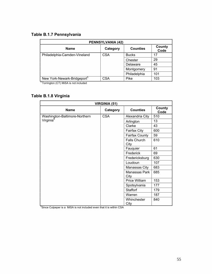
55

Table B.1.7 Pennsylvania

PENNSYLVANIA (42)


Bucks 17 Chester 29 Delaware 45 Montgomery 91

Philadelphia-Camden-Vineland CSA

Philadelphia 101 New York-Newark-Bridgeport5 CSA Pike 103

5 Torrington (CT) MiSA is not included

Table B.1.8 Virginia

VIRGINIA (51)


Alexandria City 510 Arlington 13 Clarke 43 Fairfax City 600 Fairfax County 59 Falls Church City

610

Fauquier 61 Frederick 69 Fredericksburg 630 Loudoun 107 Manassas City 683 Manassas Park City

685

Price William 153 Spotsylvania 177 Stafforf 179 Warren 187

Washington-Baltimore-Northern Virginia6

CSA

Whinchester City

840

6Since Culpeper is a MiSA is not included even that it is within CSA

56

Table B.1.9 West Virginia

WEST VIRGINIA (54)


Hampshire 27 Washington-Baltimore-Northern Virginia

CSA Jefferson 37

B.2 MID-WEST REGION Table B.2.1 Indiana

INDIANA (18)


Jasper 73 Lake 89 Newton 111

Chicago-Naperville-Michigan City

CSA

Porter 127 Boone 11 Brown 13 Hamilton 57 Hancock 59 Hendricks 63 Johnson 81 Marion 97 Morgan 109 Putnam 133

Indianapolis7 MSA

Shelby 145 Columbus MSA Bartholomew 5 Anderson MSA Madison 95

Clark 19 Floyd 43 Harrison 61

Louisville MSA

Washington 175 Dearborn 29 Franklin 47

Cincinnati-Middletown MSA

Ohio 115 7 These were considered as MSAs instead of one CSA because Indianapolis-Anderson-Columbus CSA includes Crawfordsville MiSA, and only MSAa are desired.

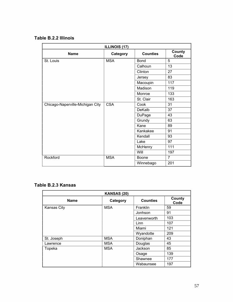
57

Table B.2.2 Illinois

ILLINOIS (17)


Bond 5 Calhoun 13 Clinton 27 Jersey 83 Macoupin 117 Madison 119 Monroe 133

St. Louis MSA

St. Clair 163 Cook 31 DeKalb 37 DuPage 43 Grundy 63 Kane 89 Kankakee 91 Kendall 93 Lake 97 McHenry 111

Chicago-Naperville-Michigan City CSA

Will 197 Boone 7 Rockford MSA Winnebago 201

Table B.2.3 Kansas

KANSAS (20)


Franklin 59 Jonhson 91 Leavenworth 103 Linn 107 Miami 121

Kansas City MSA

Wyandotte 209 St. Joseph MSA Doniphan 43 Lawrence MSA Douglas 45

Jackson 85 Osage 139 Shawnee 177

Topeka MSA

Wabaunsee 197

58

Table B.2.4 Kentucky

KENTUCKY (21)


Bullit 29 Henry 103 Jefferson 111 Meade 163 Nelson 179 Oldham 185 Shelby 211 Spencer 215

Louisville MSA

Trimble 223 Hardin 93 Elizabethtown MSA Larue 123 Boone 15 Bracken 23 Campbell 37 Gallatin 77 Grant 81 Kenton 117

Cincinnati-Middletown

Pendleton 191

Table B.2.5 Michigan

MICHIGAN (26)


Genesee 49 Lapeer 87 Livingston 93 Macomb 99 Monroe 115 Oakland 125 St. Clair 147 Washtenaw 161

Detroit-Warren-Flint CSA

Wayne 163

59

Table B.2.6 Missouri

MISSOURI (29) Name Category Counties County Code

Bates 13 Caldwell 25 Cass 37 Clay 47 Clinton 49 Jackson 95 Lafayette 107 Platte 165

Kansas City MSA

Ray 177 Andrew 3 Buchanan 21

St. Joseph MSA

DeKalb 63 Franklin 71 Jefferson 99 Lincoln 113 St. Charles 183 St. Louis City 510

St. Louis County

189

Warren 219

St. Louis8 MSA

Washington 221 8This is considered as a MSA instead of a CSA because the CSA includes the St. Francois MiSA, and only MSA are desired. The rest of the counties of this MSA are located on Illinois

60

Table B.2.7 Ohio

OHIO (39) Name Category Counties County Code

Brown 15 Butler 17 Clermont 25 Hamilton 61

Cincinnati-Middletown MSA

Warren 165 Delaware 41 Fairfield 45 Franklin 49 Licking 89 Madison 97 Morrow 117 Pickaway 129

Columbus MSA

Union 159 Cuyahoga 35 Geauga 55 Lake 85 Lorain 93

Cleveland-Elyria-Mentor MSA

Medina 103 Portage 133 Akron MSA Summit 153

Table B.2.8 Wisconsin

WISCONSIN (55) Name Category Counties County Code

Chicago-Naperville-Michigan City

CSA Kenosha 59

61

B.3 NEW ENGLAND REGION Table B.3.1 Connecticut

CONNECTICUT (9) NAME CATEGORY COUNTIES ID County

Hartford 3 Middlesex 7

Hartford-West Hartford-East Hartford

MSA

Tolland 13 Norwich-New London MSA New London 11

Table B.3.2 Connecticut

MAINE (23) NAME CATEGORY COUNTIES ID County

Bangor MSA Penobscot 19 Androscoggin 1 Cumberland 5 Sagadahoc 23

Portland-Lewiston-South Portland CSA

York 31 Table B.3.3 Massachusetts

MASSACHUSETTS (25) Not county codes needed since all are within MSAs. Only the State code is required since the query done at state level

Table B.3.4 New Hampshire

NEW HAMPSHIRE (33) NAME CATEGORY COUNTIES ID County

Manchester-Nashua MSA Hillsborough 11 Rockingham 15 Boston-Cambridge-Quincy MSA Strafford 17

62

Table B.3.5 Rhode Island

RHODE ISLAND (44) Not county codes needed since all are within MSAs. Only the State code is required since the query done at state level

Table B.3.6 Vermont

VERMONT (50) NAME CATEGORY COUNTIES ID County

Chittenden 7 Franklin 11

Burlington-South Burlingon MSA

Grand Isle 13 B.4 SOUTH REGION Table B.4.1 Alabama

ALABAMA (1) Name Category Counties ID County

Bibb 7 Blount 9 Chilton 21 Jefferson 73 Shelby 117 St. Clair 115

Birmingham-Hoover9 MSA

Walker 127 Hale 65 Greene 63

Tuscaloosa MSA

Tuscaloosa 125 Autauga 1 Elmore 51 Lowndes 85

Montgomery MSA

Montgomery 101 Gadsden MSA Etowah 55 Anniston-Oxford MSA Calhoun 15 9This is consider as a MSA instead of a CSA because within the CSA includes Cullman MiSA, and only MSAs are desired

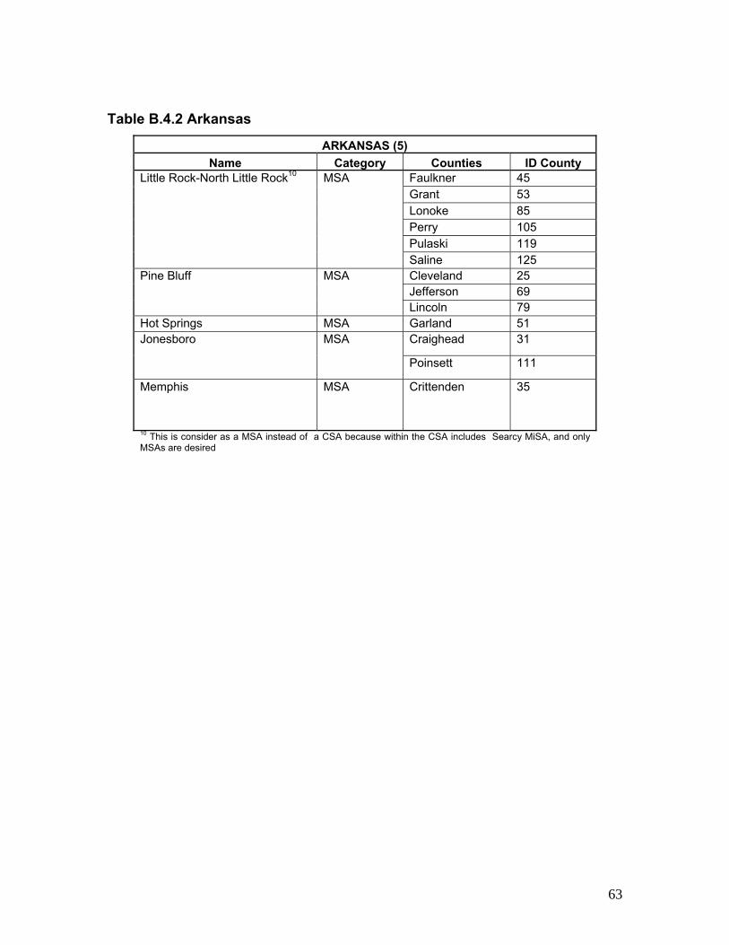
63

Table B.4.2 Arkansas

ARKANSAS (5) Name Category Counties ID County

Faulkner 45 Grant 53 Lonoke 85 Perry 105 Pulaski 119

Little Rock-North Little Rock10 MSA

Saline 125 Cleveland 25 Jefferson 69

Pine Bluff MSA

Lincoln 79 Hot Springs MSA Garland 51

Craighead 31 Jonesboro MSA

Poinsett 111

Memphis MSA Crittenden 35

10 This is consider as a MSA instead of a CSA because within the CSA includes Searcy MiSA, and only MSAs are desired

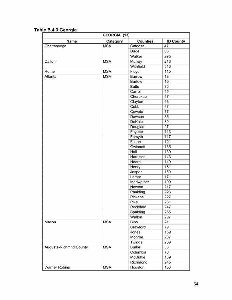
64

Table B.4.3 Georgia GEORGIA (13)

Name Category Counties ID County Catoosa 47 Dade 83

Chattanooga MSA

Walker 295 Murray 213 Dalton MSA Withfield 313

Rome MSA Floyd 115 Barrow 13 Bartow 15 Butts 35 Carroll 45 Cherokee 57 Clayton 63 Cobb 67 Coweta 77 Dawson 85 DeKalb 89 Douglas 97 Fayette 113 Forsyth 117 Fulton 121 Gwinnett 135 Hall 139 Haralson 143 Heard 149 Henry 151 Jasper 159 Lamar 171 Meriwether 199 Newton 217 Paulding 223 Pickens 227 Pike 231 Rockdale 247 Spalding 255

Atlanta MSA

Walton 297 Bibb 21 Crawford 79 Jones 169 Monroe 207

Macon MSA

Twiggs 289 Burke 33 Columbia 73 McDuffie 189

Augusta-Richmnd County MSA

Richmond 245 Warner Robins MSA Houston 153

65

Table B.4.4 Mississippi

MISSISSIPPI (28) Name Category Counties ID County

DeSoto 33 Marshall 93 Tate 137

Memphis MSA

Tunica 143 Copiah 29 Hinds 49 Madison 89 Rankin 121

Jackson11 MSA

Simpson 127 11 This is consider as a MSA instead of a CSA because within the CSA includes Yazoo City MiSA, and only MSAs are desired

Table B.4.5 North Carolina

NORTH CAROLINA (37) Name Category Counties ID County

Anson 7 Cabarrus 25 Gaston 71 Mecklenburg 119

Charlotte- Gastonia-Concord MSA

Union 179 Davie 59 Forsyth 67 Stokes 169

Winston-Salem MSA

Yadkin 197 Guilford 81 Randolph 151

Greensboro-High Point MSA

Rockingham 157 Burlington MSA Alamance 1

Chatham 37 Durham 63 Orange 135

Durham MSA

Person 145 Franklin 69 Jonhston 101

Raleigh-Cary MSA

Wake 183 Virginia Beach-Norfolk-Newport News

MSA Currituck 53

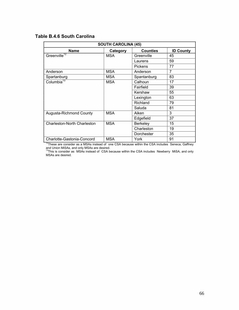
66

Table B.4.6 South Carolina

SOUTH CAROLINA (45) Name Category Counties ID County

Greenville 45 Laurens 59

Greenville12 MSA

Pickens 77 Anderson MSA Anderson 7 Spartanburg MSA Spantanburg 83

Calhoun 17 Fairfield 39 Kershaw 55 Lexington 63 Richland 79

Columbia13 MSA

Saluda 81 Aiken 3 Augusta-Richmond County MSA Edgefield 37 Berkeley 15 Charleston 19

Charleston-North Charleston MSA

Dorchester 35 Charlotte-Gastonia-Concord MSA York 91 12These are consider as a MSAs instead of one CSA because within the CSA includes Seneca, Gaffney and Union MiSAs, and only MSAs are desired. 13This is consider as MSAs instead of CSA because within the CSA includes Newberry MiSA, and only MSAs are desired.

67

Table B.4.7 Tennessee

TENNESSEE (47) Name Category Counties ID County

Cannon 15 Cheatham 21 Davidson 37 Dickson 43 Hickman 81 Macon 111 Robertson 147 Rutherford 149 Smith 159 Sumner 165 Trousdale 169 Williamson 187

Nashville-Davidson-Murfreesboro14

MSA

Wilson 189 Fayette 47 Tipton 167

Memphis MSA

Shelby 157 Hamilton 65 Marion 115

Chattanooga MSA

Sequatchie 153 Bradley 11 Cleveland MSA Polk 139

14 This is consider as a MSA instead of a CSA because within the CSA includes Columbia MiSA, and only MSAs are desired

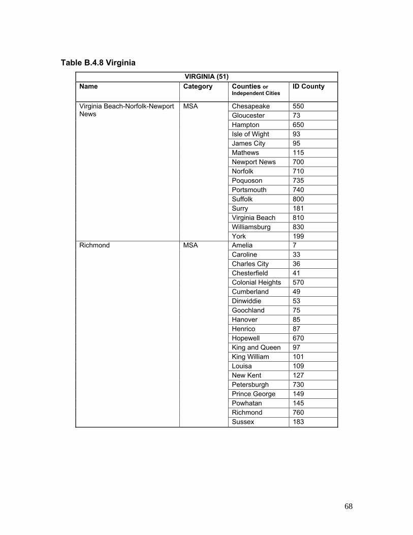
68

Table B.4.8 Virginia

VIRGINIA (51) Name Category Counties or

Independent Cities ID County

Chesapeake 550 Gloucester 73 Hampton 650 Isle of Wight 93 James City 95 Mathews 115 Newport News 700 Norfolk 710 Poquoson 735 Portsmouth 740 Suffolk 800 Surry 181 Virginia Beach 810 Williamsburg 830

Virginia Beach-Norfolk-Newport News

MSA

York 199 Amelia 7 Caroline 33 Charles City 36 Chesterfield 41 Colonial Heights 570 Cumberland 49 Dinwiddie 53 Goochland 75 Hanover 85 Henrico 87 Hopewell 670 King and Queen 97 King William 101 Louisa 109 New Kent 127 Petersburgh 730 Prince George 149 Powhatan 145 Richmond 760

Richmond MSA

Sussex 183

69

B.5 TEXAS (CASE 1) Table B.5 Texas Case 1

TEXAS(48). BIG CITIES NAME CATEGORY COUNTIES ID County

Collin 85 Dallas 113 Delta 119 Denton 121 Ellis 139 Fannin 147 Hunt 231 Johnson 251 Kaufman 257 Parker 367 Rockwall 397 Tarrant 439

Dallas-Forth Worth MSA

Wise 497 Sherman-Denison MSA Grayson 181

Bastrop 21 Caldwell 55 Hays 209 Travis 453

Austin-Round Rock MSA

Williamson 491 Austin 15 Brazoria 39 Chambers 71 Fort Bend 157 Galveston 167 Harris 201 Liberty 291 Montgomery 339 San Jacinto 407

Houston- Sugar Land-Baytown MSA

Waller 473

70

B.6 TEXAS (CASE 2) Table B.6 Texas Case 2

TEXAS (48). BIG CITIES + SAN ANTONIO + EL PASO (48) NAME CATEGORY COUNTIES ID County

Atascosa 13 Bandera 19 Bexar 29 Comal 91 Guadalupe 187 Kendall 259 Medina 325

San Antonio MSA

Wilson 493 El Paso MSA El Paso 141

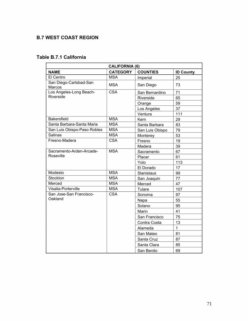
71

B.7 WEST COAST REGION Table B.7.1 California

CALIFORNIA (6) NAME CATEGORY COUNTIES ID County El Centro MSA Imperial 25 San Diego-Carlsbad-San Marcos MSA San Diego 73

San Bernardino 71 Riverside 65 Orange 59 Los Angeles 37

Los Angeles-Long Beach-Riverside

CSA

Ventura 111 Bakersfield MSA Kern 29 Santa Barbara-Santa Maria MSA Santa Barbara 83 San Luis Obispo-Paso Robles MSA San Luis Obispo 79 Salinas MSA Monterey 53

Fresno 19 Fresno-Madera CSA Madera 39 Sacramento 67 Placer 61 Yolo 113

Sacramento-Arden-Arcade-Roseville

MSA

El Dorado 17 Modesto MSA Stanislaus 99 Stockton MSA San Joaquin 77 Merced MSA Merced 47 Visalia-Porterville MSA Tulare 107

Sonoma 97 Napa 55 Solano 95 Marin 41 San Francisco 75 Contra Costa 13 Alameda 1 San Mateo 81 Santa Cruz 87 Santa Clara 85

San Jose-San Francisco-Oakland

CSA

San Benito 69

72

Table B.7.2 Oregon

OREGON (41) NAME CATEGORY COUNTIES ID County

Polk 53 Salem MSA Marion 47 Columbia 9 Washington 67 Yamhill 71 Clackamas 5

Portland-Vancouver-Beaverton

MSA

Multinomah 51 Corvallis MSA Benton 3

Eugene-Springfield MSA Lane 39 Bend MSA Deschuttes 17

Table B.7.3 Washington

WASHINGTON (53) NAME CATEGORY COUNTIES ID County

Snohomish 61 King 33

Seattle-Tacoma-Bellevue MSA

Pierce 53 Bremerton-Silverdale MSA Kitsap 35

Clark 11 Portland-Vancouver-Beaverton

MSA

Skamania 59

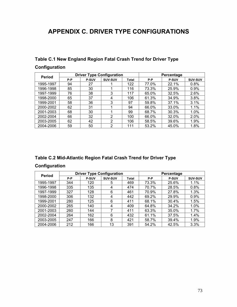
73

APPENDIX C. DRIVER TYPE CONFIGURATIONS Table C.1 New England Region Fatal Crash Trend for Driver Type Configuration

Driver Type Configuration Percentage Period P-P P-SUV SUV-SUV Total P-P P-SUV SUV-SUV

1995-1997 94 27 1 122 77.0% 22.1% 0.8% 1996-1998 85 30 1 116 73.3% 25.9% 0.9% 1997-1999 76 38 3 117 65.0% 32.5% 2.6% 1998-2000 65 37 4 106 61.3% 34.9% 3.8% 1999-2001 58 36 3 97 59.8% 37.1% 3.1% 2000-2002 62 31 1 94 66.0% 33.0% 1.1% 2001-2003 68 30 1 99 68.7% 30.3% 1.0% 2002-2004 66 32 2 100 66.0% 32.0% 2.0% 2003-2005 62 42 2 106 58.5% 39.6% 1.9% 2004-2006 59 50 2 111 53.2% 45.0% 1.8%

Table C.2 Mid-Atlantic Region Fatal Crash Trend for Driver Type Configuration


1995-1997 344 120 5 469 73.3% 25.6% 1.1% 1996-1998 335 135 4 474 70.7% 28.5% 0.8% 1997-1999 327 128 6 461 70.9% 27.8% 1.3% 1998-2000 306 132 4 442 69.2% 29.9% 0.9% 1999-2001 280 125 6 411 68.1% 30.4% 1.5% 2000-2002 265 140 4 409 64.8% 34.2% 1.0% 2001-2003 260 144 7 411 63.3% 35.0% 1.7% 2002-2004 264 162 6 432 61.1% 37.5% 1.4% 2003-2005 247 166 8 421 58.7% 39.4% 1.9% 2004-2006 212 166 13 391 54.2% 42.5% 3.3%

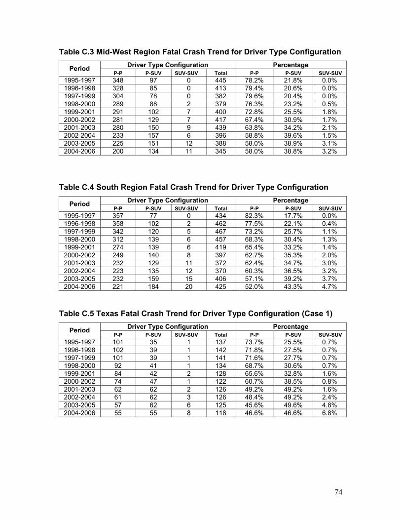
74

Table C.3 Mid-West Region Fatal Crash Trend for Driver Type Configuration Driver Type Configuration Percentage Period

P-P P-SUV SUV-SUV Total P-P P-SUV SUV-SUV 1995-1997 348 97 0 445 78.2% 21.8% 0.0% 1996-1998 328 85 0 413 79.4% 20.6% 0.0% 1997-1999 304 78 0 382 79.6% 20.4% 0.0% 1998-2000 289 88 2 379 76.3% 23.2% 0.5% 1999-2001 291 102 7 400 72.8% 25.5% 1.8% 2000-2002 281 129 7 417 67.4% 30.9% 1.7% 2001-2003 280 150 9 439 63.8% 34.2% 2.1% 2002-2004 233 157 6 396 58.8% 39.6% 1.5% 2003-2005 225 151 12 388 58.0% 38.9% 3.1% 2004-2006 200 134 11 345 58.0% 38.8% 3.2%

Table C.4 South Region Fatal Crash Trend for Driver Type Configuration


1995-1997 357 77 0 434 82.3% 17.7% 0.0% 1996-1998 358 102 2 462 77.5% 22.1% 0.4% 1997-1999 342 120 5 467 73.2% 25.7% 1.1% 1998-2000 312 139 6 457 68.3% 30.4% 1.3% 1999-2001 274 139 6 419 65.4% 33.2% 1.4% 2000-2002 249 140 8 397 62.7% 35.3% 2.0% 2001-2003 232 129 11 372 62.4% 34.7% 3.0% 2002-2004 223 135 12 370 60.3% 36.5% 3.2% 2003-2005 232 159 15 406 57.1% 39.2% 3.7% 2004-2006 221 184 20 425 52.0% 43.3% 4.7%

Table C.5 Texas Fatal Crash Trend for Driver Type Configuration (Case 1)


1995-1997 101 35 1 137 73.7% 25.5% 0.7% 1996-1998 102 39 1 142 71.8% 27.5% 0.7% 1997-1999 101 39 1 141 71.6% 27.7% 0.7% 1998-2000 92 41 1 134 68.7% 30.6% 0.7% 1999-2001 84 42 2 128 65.6% 32.8% 1.6% 2000-2002 74 47 1 122 60.7% 38.5% 0.8% 2001-2003 62 62 2 126 49.2% 49.2% 1.6% 2002-2004 61 62 3 126 48.4% 49.2% 2.4% 2003-2005 57 62 6 125 45.6% 49.6% 4.8% 2004-2006 55 55 8 118 46.6% 46.6% 6.8%

75

Table C.6 Texas Fatal Crash Trend for Driver Type Configuration (Case 2) Driver Type Configuration Percentage Period

P-P P-SUV SUV-SUV Total P-P P-SUV SUV-SUV 1995-1997 117 40 1 158 74.1% 25.3% 0.6% 1996-1998 118 45 1 164 72.0% 27.4% 0.6% 1997-1999 116 43 1 160 72.5% 26.9% 0.6% 1998-2000 104 49 2 155 67.1% 31.6% 1.3% 1999-2001 96 51 3 150 64.0% 34.0% 2.0% 2000-2002 91 60 2 153 59.5% 39.2% 1.3% 2001-2003 81 75 4 160 50.6% 46.9% 2.5% 2002-2004 84 71 5 160 52.5% 44.4% 3.1% 2003-2005 75 71 8 154 48.7% 46.1% 5.2% 2004-2006 71 61 8 140 50.7% 43.6% 5.7%

Table C.7 West Coast Region Fatal Crash Trend for Driver Type Configuration


1995-1997 345 128 1 474 72.8% 27.0% 0.2% 1996-1998 324 131 3 458 70.7% 28.6% 0.7% 1997-1999 319 135 5 459 69.5% 29.4% 1.1% 1998-2000 287 154 9 450 63.8% 34.2% 2.0% 1999-2001 281 183 12 476 59.0% 38.4% 2.5% 2000-2002 280 190 16 486 57.6% 39.1% 3.3% 2001-2003 309 191 18 518 59.7% 36.9% 3.5% 2002-2004 293 181 21 495 59.2% 36.6% 4.2% 2003-2005 274 181 19 474 57.8% 38.2% 4.0% 2004-2006 238 185 18 441 54.0% 42.0% 4.1%

Safety Externalities of SUVs on Passenger Cars: An ... · Safety Externalities of SUVs on Passenger...

Documents

Transcript of Safety Externalities of SUVs on Passenger Cars: An ... · Safety Externalities of SUVs on Passenger...