Safe Policy Iteration: A Monotonically Improving ...
83
Journal of Machine Learning Research 22 (2021) 1-83 Submitted 8/19; Revised 12/20; Published 4/21 Safe Policy Iteration: A Monotonically Improving Approximate Policy Iteration Approach Alberto Maria Metelli [email protected] DEIB, Politecnico di Milano Milano, Italy Matteo Pirotta [email protected] Facebook AI Research Paris, France Daniele Calandriello [email protected] Istituto Italiano di Tecnologia Genova, Italy Marcello Restelli [email protected] DEIB, Politecnico di Milano Milano, Italy Editor: Peter Auer Abstract This paper presents a study of the policy improvement step that can be usefully exploited by approximate policy–iteration algorithms. When either the policy evaluation step or the policy improvement step returns an approximated result, the sequence of policies produced by policy iteration may not be monotonically increasing, and oscillations may occur. To address this issue, we consider safe policy improvements, i.e., at each iteration, we search for a policy that maximizes a lower bound to the policy improvement w.r.t. the current policy, until no improving policy can be found. We propose three safe policy–iteration schemas that differ in the way the next policy is chosen w.r.t. the estimated greedy policy. Besides being theoretically derived and discussed, the proposed algorithms are empirically evaluated and compared on some chain-walk domains, the prison domain, and on the Blackjack card game. Keywords: Reinforcement Learning, Approximate Dynamic Programming, Approximate Policy Iteration, Policy Oscillation, Policy Chattering, Markov Decision Process 1. Introduction Markov Decision Processes (MDPs) are widely used to model sequential decision-making problems under uncertainty (Puterman, 2014). In the last decades, a large body of re- search from control theory, operation research, and artificial intelligence has been devoted to the solution of MDPs. When a model of the environment is available, MDPs can be solved by dynamic programming algorithms or linear programming. On the contrary, when no or little prior knowledge about the model is known or when the problem is too com- plex for an exact solution, approximate methods need to be considered, like those studied ©2021 Alberto Maria Metelli, Matteo Pirotta, Daniele Calandriello, Marcello Restelli. License: CC-BY 4.0, see https://creativecommons.org/licenses/by/4.0/. Attribution requirements are provided at http://jmlr.org/papers/v22/19-707.html.
Transcript of Safe Policy Iteration: A Monotonically Improving ...

Journal of Machine Learning Research 22 (2021) 1-83 Submitted 8/19; Revised 12/20; Published 4/21
Safe Policy Iteration: A Monotonically ImprovingApproximate Policy Iteration Approach
Alberto Maria Metelli [email protected], Politecnico di MilanoMilano, Italy
Matteo Pirotta [email protected] AI ResearchParis, France
Daniele Calandriello [email protected] Italiano di TecnologiaGenova, Italy
Marcello Restelli [email protected]
DEIB, Politecnico di Milano
Milano, Italy
Editor: Peter Auer
Abstract
This paper presents a study of the policy improvement step that can be usefully exploitedby approximate policy–iteration algorithms. When either the policy evaluation step or thepolicy improvement step returns an approximated result, the sequence of policies producedby policy iteration may not be monotonically increasing, and oscillations may occur. Toaddress this issue, we consider safe policy improvements, i.e., at each iteration, we searchfor a policy that maximizes a lower bound to the policy improvement w.r.t. the currentpolicy, until no improving policy can be found. We propose three safe policy–iterationschemas that differ in the way the next policy is chosen w.r.t. the estimated greedy policy.Besides being theoretically derived and discussed, the proposed algorithms are empiricallyevaluated and compared on some chain-walk domains, the prison domain, and on theBlackjack card game.
Keywords: Reinforcement Learning, Approximate Dynamic Programming, ApproximatePolicy Iteration, Policy Oscillation, Policy Chattering, Markov Decision Process
1. Introduction
Markov Decision Processes (MDPs) are widely used to model sequential decision-makingproblems under uncertainty (Puterman, 2014). In the last decades, a large body of re-search from control theory, operation research, and artificial intelligence has been devotedto the solution of MDPs. When a model of the environment is available, MDPs can besolved by dynamic programming algorithms or linear programming. On the contrary, whenno or little prior knowledge about the model is known or when the problem is too com-plex for an exact solution, approximate methods need to be considered, like those studied
©2021 Alberto Maria Metelli, Matteo Pirotta, Daniele Calandriello, Marcello Restelli.
License: CC-BY 4.0, see https://creativecommons.org/licenses/by/4.0/. Attribution requirements are providedat http://jmlr.org/papers/v22/19-707.html.

Metelli, Pirotta, Calandriello, and Restelli
in the Reinforcement Learning (RL, Sutton and Barto, 2018) and Approximate DynamicProgramming (ADP, Bertsekas, 2011).
In this paper, we focus on approaches derived from Policy Iteration (PI, Howard, 1960),one of the two main classes of dynamic programming algorithms to solve MDPs. PI isan iterative algorithm that alternates between two steps: policy evaluation and policy im-provement. At each iteration, the current policy πk is evaluated computing the action–valuefunction Qπk and the new policy πk+1 is generated by taking the greedy policy w.r.t. Qπk ,i.e., the policy that in each state takes the best action according to Qπk . Policy iterationgenerates a sequence of monotonically improving policies that reaches the optimal policy ina finite number of iterations (Ye, 2011; Scherrer, 2013a).
When either Qπk or the corresponding greedy policy πk+1 cannot be computed exactly,Approximate Policy Iteration (API, Bertsekas, 2011) algorithms need to be considered. Alarge number of methods tackling this problem have been proposed in the literature (Scher-rer, 2014). The standard API (Bertsekas and Tsitsiklis, 1996) simply computes the greedypolicy w.r.t. to the estimated value function Qπk . However, in this case, the approximatelygreedy policy πk+1 may perform worse than πk, leading, thus, to policy oscillation phe-nomena (Bertsekas, 2011; Wagner, 2011). Empirically, the value Qπk rapidly improves inthe initial iterations, then gets stuck or oscillates without any further policy improvement(named stationary phase Munos, 2003). Most API studies and algorithms focus on reducingthe approximation error in the policy evaluation step (Lagoudakis and Parr, 2003a; Munos,2005; Lazaric et al., 2010; Gabillon et al., 2011), and, then, perform policy improvement bytaking the relative greedy policy. However, the quality of the sequence of generated policiesmay oscillate or diverge when the policy evaluation is approximated, independently of thepolicy evaluation method (Bertsekas and Tsitsiklis, 1996; Bertsekas, 2011).
Almost all the API algorithms intrinsically implement a generalized policy iterationscheme (Sutton and Barto, 2018) because the improvement of the policy is performed overan incomplete estimate of the value functions. This idea was used in Scherrer et al. (2012);Scherrer (2013b) to generalize over Value Iteration (VI) and PI methods at the cost ofadditional free parameters.
It has been pointed out that the key source of this oscillation phenomena is the discon-tinuity introduced by the greedy improvement (De Farias and Van Roy, 2000; Perkins andPendrith, 2002; Perkins and Precup, 2002). Approximate Linear Programming (de Fariasand Roy, 2003) solves the RL problem in one shot, but typically assumes the knowledgeof the transition model and the approximation comes from the fact that the value functionis represented as a function approximator (e.g., linear in a vector of known features). Asnoticed in the early stages of RL (Singh et al., 1994), stochastic policies may represent thesolution to many issues. A class of approaches deals with the oscillation phenomena byproposing converging algorithms that exploit smaller updates (soft updates) in the space ofstochastic policies, instead of iterating on a sequence of greedy policies computed on ap-proximated action–value functions (Perkins and Precup, 2002; Kakade and Langford, 2002;Lagoudakis and Parr, 2003b; Wagner, 2011; Azar et al., 2012). The idea is that the action–value function of a policy π can produce a good estimate of the performance of anotherpolicy π′ when the two policies give rise to similar state distributions. This condition canbe guaranteed when the policies themselves are similar. Incremental policy updates arealso considered in the related class of policy gradient algorithms (e.g., Sutton et al., 1999;
2

Safe Policy Iteration
Kakade, 2001; Peters et al., 2005). These methods share a common rationale based onmanaging the trade–off between jumping to the greedy policy according to the currentlyestimated action–value function and remaining close to the current policy avoiding too un-certain updates. From an intuitive point of view, the more we trust our value functionestimate, the more we can move far from the current policy. This very simple idea has beendeveloped in several works and for different purposes (e.g., Pirotta et al., 2013a; Abbasi-Yadkori et al., 2016; Ghavamzadeh et al., 2016; Papini et al., 2017; Metelli et al., 2018) andit represents the theoretical grounding of some of the most successful RL algorithms (e.g.,Schulman et al., 2015).
Other works focus on the “optimistic” or “modified” PI approach. This variant of policyiteration is based on an approximate evaluation of the preceding policy obtained by applyingthe Bellman operator a finite number of times. While Scherrer et al. (2012) have derived aconvergence and finite samples analysis for the “optimistic” policy iteration generalizationof the classification–based policy iteration, Wagner (2013) has investigated the connectionbetween optimistic policy iteration and natural actor–critic algorithms. They have shownthat the natural actor–critic algorithm for Gibbs policy is a special case of optimistic policyiteration. In addition, they suggested that it is possible to get convergence guarantees forPI approaches exploiting the theory behind gradient methods. However, they proved that,while having the potential of overcoming policy oscillation, Gibbs soft–greedy value functionapproaches never converge to the optimal policy.
Another research line focuses on the exploitation of non–stationary policy sequences(Scherrer and Lesner, 2012). The authors propose an algorithm that, at each iteration, ap-proximates the value function of a policy that loops over the last m greedy policies generatedby the algorithm (possibly also considering all the policies generated from the beginning ofthe algorithm). Thus, the resulting policy is non–stationary and has a regularizing effect onthe learning process. They show that, by employing non–stationary policies, it is possibleto obtain better convergence rates (Scherrer and Lesner, 2012; Lesner and Scherrer, 2013).The methods have also been applied to the case of modified PI (Lesner and Scherrer, 2015).
Recently, one research line has imported the classical idea of delaying the backup op-eration, successfully applied in the famous TD methods (Sutton and Barto, 2018), to thePI framework by defining the multi–step greedy improvements (Efroni et al., 2018a). Theseworks overcome the 1–step greedy update by defining an h–greedy policy (h ≥ 1) as thepolicy that, from every state, is optimal for h time steps. This new improvement operatoramounts to solve an h–horizon optimal control problem, reducing to the standard 1–stepoperator for h = 1, converges to the optimal policy in a number of iterations that decreaseswith h (Efroni et al., 2018a). Similarly to the TD(λ) case, it is possible to mix differenthorizons using a parameter to tradeoff between the 1–step greedy improvement and morefar–sighted updates (Efroni et al., 2018a). The idea is then extended to the approximatesetting in Efroni et al. (2018b).
In this paper, we limit our scope to the classical API approaches, built on station-ary policies1 and, following the approach of Conservative Policy Iteration (CPI, Kakadeand Langford, 2002), which adopts soft updates to avoid oscillation phenomena, and re-cently extended to use deep architectures (Vieillard et al., 2020). We extend CPI Kakade
1. In the case of infinite–horizon γ–discounted MDPs, it is known that there exists a stationary optimalpolicy.
3

Metelli, Pirotta, Calandriello, and Restelli
and Langford (2002) by introducing a tighter lower bound on the performance improve-ment, that allows designing API algorithms useful both in model–free contexts and whena restricted subset of policies is considered. These algorithms produce a sequence of mono-tonically improving policies and are characterized by a faster-improving rate compared toCPI. Furthermore, we devise an update schema that makes use of per–state combinationcoefficients and a novel generalization, not present in Pirotta et al. (2013b), that employsper–state–action coefficients.
The main contributions of this paper are theoretical, algorithmic, and experimentalconsisting in:
1. the introduction of new, more general lower bounds on the policy improvement, tighterthan the one presented in Pirotta et al. (2013b) (Section 3);
2. the proposal of three approximate policy–iteration algorithms whose performance im-provement moves toward the estimated greedy policy by maximizing the policy im-provement bounds. The first two of them have already been presented in Pirottaet al. (2013b), while the third and more general is novel and presented here in aunified framework (Section 4);
3. a complete PAC analysis of the approximate version of the presented algorithms, withfinite–sample improvement guarantees for the single iteration (Section 5);
4. an empirical evaluation and comparison of the proposed algorithms with related ap-proaches (Section 6).
The rest of the paper is organized as follows. Section 2 introduces notation and thenecessary background. Section 3 derives the bounds on the difference between the per-formance of two policies and provides the policy improvement bounds. Based on thesebounds, we present the exact algorithms in Section 4 and the approximated in Section 5. InSection 6, the algorithms are empirically evaluated and compared with other approximatepolicy–iteration algorithms on several variants of the chain–walk domain (Lagoudakis andParr, 2003a), Prison environment (Azar et al., 2012), and in a simplified version of theBlackjack (Dutech et al., 2005).
2. Preliminaries
In this section, we report the essential background that will be employed in the remainderof the paper.
Markov Decision Processes A discrete–time finite Markov Decision Process (MDP,Puterman, 2014) is defined as a 6–tuple M = (S,A,P,R, γ, µ), where S is a finite setof states, A is a finite set of actions, P is a Markovian transition model where P(s′|s, a)is the probability of making a transition to state s′ when taking action a from state s,R : S × A → [0, 1] is the reward function, such that R(s, a) is the expected immediatereward for the state–action pair (s, a), γ ∈ [0, 1) is the discount factor for future rewards,and µ is the initial state distribution. The policy of an agent is characterized by a densitydistribution π(a|s) that specifies the probability of taking action a in state s. When thepolicy is deterministic, with little abuse of notation, we use π(s) to denote the action
4
Safe Policy Iteration
prescribed in state s. We consider infinite–horizon problems where the future rewards areexponentially discounted with γ. For each state s, we define the utility of following astationary policy π as:
V π(s) = Eat∼π(·|st)
st+1∼P(·|st,at)
[+∞∑
t=0
γtR(st, at)|s0 = s
].
It is known that V π is the unique solution of the following recursive (Bellman) equation:
V π(s) =∑
a∈Aπ(a|s)
(R(s, a) + γ
∑
s′∈SP(s′|s, a)V π(s′)
).
Policies can be ranked by their expected discounted reward starting from the state distri-bution :
Jπ =∑
s∈Sµ(s)V π(s) =
1
1− γ∑
s∈Sdπ(s)
∑
a∈Aπ(a|s)R(s, a),
where dπ(s) = (1−γ)∑∞
t=0 γt Pr(st = s|π,M) is the γ–discounted future state distribution
for a starting state distribution (Sutton et al., 1999). Solving an MDP means to find apolicy π∗ that maximizes the expected long–term reward: π∗ ∈ arg maxπ∈ΠSR Jπ, where ΠSR
is the set of stationary Markovian randomized policies. For any MDP, there exists at leastone deterministic optimal policy that simultaneously maximizes V π(s), ∀s ∈ S, i.e., existsπ∗ ∈ ΠSD, where ΠSD is the set of stationary Markovian deterministic policies (Puterman,2014). For control purposes, it is more convenient to consider the action–value functionQπ(s, a), i.e., the value of taking action a in state s and following a policy π thereafter:
Qπ(s, a) = R(s, a) + γ∑
s′∈SP(s′|s, a)
∑
a′∈Aπ(a′|s′)Qπ(s′, a′).
Given Qπ(s, a), we define a greedy policy as π+(s) ∈ arg maxa∈AQπ(s, a). Furthermore, we
define the advantage function as:
Aπ(s, a) = Qπ(s, a)− V π(s),
that quantifies the convenience of performing action a in state s instead of following policy π.Furthermore, for each state s, we define the advantage of a policy π′ over policy π as Aπ
′π (s) =∑
a∈A π′(a|s)Aπ(s, a) and, following what done by Kakade and Langford (2002), we define
its expected value w.r.t. the γ–discounted state distribution dπ as Aπ′π =∑
s∈S dπ(s)Aπ
′π (s).
Notation Vectors are assumed to be columns and are denoted with lowercase boldletters, like v; while matrices are denoted with upper case bold letters, like M. For brevity,in the following, we will use matrix notation, where I denotes the identity matrix and eis a column vector of all ones (with sizes apparent from the context). Given a (column)vector v, vT denotes the corresponding row vector. Whenever necessary, a d–dimensionalvector v will be treated as a d × 1 matrix, and, symmetrically, a row vector vT will betreated as a 1 × d matrix. Given a matrix M, MT denotes its transpose, and, given anon–singular square matrix M, M−1 denotes its inverse. For brevity, M−T =
(MT)−1
.For a vector v, we indicate with v(i) its i–th component and for a matrix M, we indicate
5

Metelli, Pirotta, Calandriello, and Restelli
with M(i, j) the component at row i and column j. Let p ∈ [1,∞), we define the Lp–
norm of a d–dimensional vector v as ‖v‖pp =∑d
i=1 |v(i)|p. The L∞–norm of v is givenby ‖v‖∞ = maxi∈{1,...,d} |v(i)|. Moreover, we define the span seminorm of v as sp(v) =maxi∈{1,...,d} v(i) − mini∈{1,...,d} v(i). We consider the Lp–norms of matrices induced bythe corresponding vector norm, defined as ‖M‖p = supv : ‖v‖p≤1 ‖Mv‖p. In particular, the
L1–norm ‖M‖1 of a matrix M is its maximum absolute column sum, while its L∞–norm‖M‖∞ is its maximum absolute row sum. It follows that ‖M‖1 =
∥∥MT∥∥∞ (Petersen and
Pedersen, 2012). If v is a probability column vector of size n and M is an n ×m matrix,we indicate with ‖M‖p,v the expectation of the Lp–norm of the columns of M taken under
v, i.e., ‖M‖p,v =∑n
i=1 v(i)(∑m
j=1 |M(i, j)|p)1/p
.
Matrix Notation for MDPs Using matrix notation, we can rewrite previous equationsas follows (e.g., Puterman, 2014; Wang et al., 2007):
vπ = π (r + γPvπ) = rπ + γPπvπ = (I− γPπ)−1 rπ
qπ = r + γPπqπ = r + γPvπ
dπ = (1− γ)µ + γPπTdπ = (1− γ)(I− γPπ)−Tµ
Jπ = µTvπ = µT (I− γPπ)−1 rπ =1
1− γdπTrπ
Aπ′π = dπTπ′aπ = dπTaπ
′π ,
(1)
where Jπ and Aπ′π are scalars, vπ, rπ, dπ, µ, and aπ′π are vectors of size |S|, qπ, r, and aπ
are vectors of size |S||A|, P is a stochastic matrix of size (|S||A| × |S|) that contains thetransition model of the process P((s, a), s′) = P(s′|s, a), π is a stochastic matrix of size(|S| × |S||A|) that describes policy π:
π(s, (s′, a)) =
{π(a|s) if s′ = s
0 otherwise,
and Pπ = πP is a stochastic matrix |S| × |S| that represents the state transition matrixunder policy π, i.e., Pπ(s′|s) =
∑a∈A P(s′|s, a)π(a|s).
3. Bound on Policy Improvement
This section is devoted to the study of the performance improvement Jπ′ − Jπ of a policy
π′ over a policy π given the policy advantage function Aπ′π . Specifically, we will present
two lower bounds of the improvement Jπ′ − Jπ. The first bound (Theorem 3) is tighter,
but it is hard to optimize due to the presence of quantities that are typically unknown.For this reason, it will be employed with USPI only. The second bound (Corollary 4) is arelaxation of the previous one, allows a more straightforward optimization and it will beused for SSPI and SASPI. The presented bounds are tighter compared to that by Kakadeand Langford (2002) and Pirotta et al. (2013b).2 As we will see, Aπ
′π can provide a good
estimate of Jπ′only when the two policies π and π′ visit the states with similar probabilities,
2. A better bound allows faster improving rates while preserving the property of having a monotonicallyimproving sequence of policies.
6

Safe Policy Iteration
i.e., dπ′ ' dπ. The following lemma provides an upper bound to the difference between the
two γ–discounted future state distributions.
Lemma 1. Let π and π′ be two stationary policies for an infinite horizon MDPM. The L1–norm of the difference between their γ–discounted future state distributions under startingstate distribution µ can be upper bounded as follows:
∥∥∥dπ′ − dπ∥∥∥
1≤ γ
1− γ∥∥π′ − π
∥∥1,dπ
.
Proof To prove the lemma, we rewrite the difference dπ′T − dπT as follows:
dπ′T − dπT = (1− γ)µT + γdπ
′TPπ′ −
((1− γ)µT + γdπTPπ
)
= γdπ′TPπ′ − γdπTPπ
= γ(dπ′T − dπT
)Pπ′ + γdπT
(Pπ′ −Pπ
)
= γdπT(Pπ′ −Pπ
)(I− γPπ′
)−1,
where the first equality follows from the convergence of Neumann series (e.g., Wanget al., 2007; Pirotta et al., 2013b). We restate here the result:
dπ = (1− γ)
[+∞∑
t=0
(γπP)t]T
µ = (1− γ)µ +
[+∞∑
t=1
(γPπ)t]T
µ
= (1− γ)µ +
[+∞∑
τ=0
(γPπ)τ+1
]Tµ = (1− γ)µ + (γPπ)T
[+∞∑
τ=0
(γPπ)τ]T
µ
= (1− γ)µ + γPπTdπ.
It is worth to notice that the inverse of matrix I− γPπ′ exists for any γ < 1 since Pπ′
has the maximum eigenvalue equal to 1 being a stochastic matrix (Suzuki, 1976).
By recalling that dπT(Pπ′ −Pπ
)is a row vector, we derive the following inequality
that will be employed for the L1–norm bound:
∥∥∥dπT(Pπ′ −Pπ
)∥∥∥∞
=∑
s′∈S
∣∣∣∣∣∑
s∈Sdπ(s)
(Pπ′(s′|s)− Pπ(s′|s)
)∣∣∣∣∣
≤∑
s∈Sdπ(s)
∑
s′∈S
∣∣∣Pπ′(s′|s)− Pπ(s′|s)∣∣∣
=∑
s∈Sdπ(s)
∑
s′∈S
∣∣∣∣∣∑
a∈AP(s′|s, a)
(π′(a|s)− π(a|s)
)∣∣∣∣∣
≤∑
s∈Sdπ(s)
∑
a∈A
∣∣π′(a|s)− π(a|s)∣∣ ∑
s′∈SP(s′|s, a)
=1
(P.1)
7

Metelli, Pirotta, Calandriello, and Restelli
≤∑
s∈Sdπ(s)
∥∥π′(·|s)− π(·|s)∥∥
1, (P.2)
where line (P.1) derives from pushing the absolute value inside the summation and line (P.2)is obtained from the definition of L1–norm. From the first equation, the bound on the L1–
norm follows recalling that dπ′ − dπ is a column vector and, consequently, dπ
′T − dπT is arow vector:
∥∥∥dπ′ − dπ∥∥∥
1=∥∥∥dπ′T − dπT
∥∥∥∞
≤ γ∥∥∥dπT
(Pπ′ −Pπ
)∥∥∥∞
∥∥∥∥(I− γPπ′
)−1∥∥∥∥∞
≤ γ
1− γ∥∥π′ − π
∥∥1,dπ
.
For this part of the proof, we have exploited the consistency of the L∞–norm. In thelast equality, we have used the notion that dπ is a probability vector and observed that∥∥∥∥(I− γPπ′
)−1∥∥∥∥∞
= 11−γ .
As a further step to prove the main theorem, it is useful to rewrite the difference betweenthe performance of policy π′ and the one of policy π as a function of the policy advantagefunction Aπ
′π .
Lemma 2. (Kakade and Langford, 2002) For any stationary policies π and π′ and anystarting state distribution µ:
Jπ′ − Jπ =
1
1− γdπ′Taπ
′π .
Unfortunately, computing the improvement of policy π′ w.r.t. to π using the previouslemma is very expensive, since it requires estimating dπ
′for each candidate π′. In the
following, we will provide a bound to the policy improvement and we will show how it ispossible to find a policy π′ that optimizes its value.
Theorem 3. For any stationary policies π and π′ and any starting state distribution µ,given any baseline policy πb, the difference between the performance of π′ and the one of πcan be lower bounded as follows:
Jπ′ − Jπ ≥ 1
1− γdπbTaπ
′π −
γ
(1− γ)2
∥∥π′ − πb∥∥
1,dπb
sp(aπ′π
)
2.
Proof The proof can be obtained starting from Lemma 2:
(1− γ)(Jπ′ − Jπ
)= dπ
′Taπ′π = dπbTaπ
′π +
(dπ′T − dπbT
)aπ′π
≥ dπbTaπ′π −
∣∣∣∣(dπ′ − dπb
)Taπ′π
∣∣∣∣ (P.3)
8

Safe Policy Iteration
≥ dπbTaπ′π −
∥∥∥dπ′ − dπb∥∥∥
1
sp(aπ′π
)
2(P.4)
≥ dπbTaπ′π −
γ
1− γ∥∥π′ − πb
∥∥1,dπb
sp(aπ′π
)
2. (P.5)
Statement (P.3) is a simple mathematical manipulation (a + b ≥ a − |b|, ∀a, b ∈ R),while the inequality (P.4) follows from Lemma 23 since c = dπ
′ − dπb is a vector satisfying
cTe = (dπ′ − dπb)
Te = 1 − 1 = 0. The theorem is proved in (P.5) by exploiting the bound
in Corollary 1.
The theorem is presented for a general baseline policy πb that, ideally, is employed tocollect the samples. In principle, πb can be different from both π and π′, although, typically,we select πb = π. The bound is the sum of two terms: the advantage of policy π′ over policyπ averaged according to the distribution induced by policy πb and a penalization term thatis a function of the discrepancy between policy π′ and policy πb and the range of variabilityof the advantage function Aπ
′π .3
Remark 1 (Comparison with Pirotta et al., 2013b). The bound presented in Theorem 3strictly improves Theorem 3.5 in Pirotta et al. (2013b), since the L∞–norm between thepolicies π′ and π has been replaced with an expectation taken w.r.t. to the γ–discountedstationary distribution dπ of the state–wise L1–norms. Indeed:
∥∥π′ − πb∥∥
1,dπb≤∥∥π′ − πb
∥∥∞ .
Since the bound provided by Pirotta et al. (2013b) was already tight (being an improvementover CPI), it follows that our bound is tight as well. A similar derivation was previouslyprovided in Achiam et al. (2017, Corollary 1) and Metelli et al. (2018, Corollary 3.1). Nowwe introduce a looser but simplified version of the bound in Theorem 3 that will be usefullater.
Corollary 4. For any stationary policies π and π′ and any starting state distribution µ, thedifference between the performance of π′ and the one of π can be lower bounded as follows:
Jπ′ − Jπ ≥ 1
1− γAπ′π −
γ
(1− γ)2
∥∥π′ − π∥∥2
∞‖qπ‖∞
2.
For completeness, we mention that a different (looser) bound on the policy difference innorm can be obtained by using Pinsker’s inequality (Csiszar and Korner, 2011) stating that
∥∥π′ − π∥∥
1,dπ= Es∼dπb
[‖π(·|s)− πb(·|s)‖1
]≤√
1
2Es∼dπb
[DKL(π(·|s)‖πb(·|s))
].
This bound was initially used in Pirotta et al. (2013a) to derive a simplified lower–bound forparametrized policies and it has been adopted frequently in the literature after that (e.g.,Schulman et al., 2015; Achiam et al., 2017; Papini et al., 2017).
3. We tried to keep Theorem 3 as general as possible to favor its reuse in different contexts. Nonetheless,in the following, we will consider the particular case where πb is equal to π. The possibility of selectinga suitable πb 6= π opens new and interesting lines of research that are out of the scope of this paper.
9

Metelli, Pirotta, Calandriello, and Restelli
4. Exact Safe Policy Iteration
As we have already mentioned, Conservative Policy Iteration (CPI) approach successfullyaims at overcoming policy degradation issues in approximate contexts. Indeed, while PIalgorithms, moving from a greedy policy to another, guarantees to improve the perfor-mance at each iteration until convergence to the optimal policy only when no approxi-mation is involved, the CPI algorithm performs a more conservative improvement step toensure monotonically increasing policy performance even in the approximate setting. Inthis framework, following the approach of CPI (Kakade and Langford, 2002), we propose anew set of techniques, called Safe Policy Iteration (SPI) algorithms (Pirotta et al., 2013b).
The idea is to produce a sequence of monotonically improving policies and stop whenno improvement can be guaranteed. The policy improvement step is a trade-off betweenthe current policy π and a target policy π according to π′ = απ + (1 − α)π, where thetrade-off coefficient α ∈ [0, 1] results from a maximization of a lower bound on the policyimprovement. The main benefit of exploiting SPI methods instead of CPI one is quantifiablein a faster convergence to the optimal solution, due to a maximization of a better lowerbounds w.r.t. that of CPI.
In the following, we analyze the exact case (in which the value functions are knownwithout approximation) and we propose three safe policy-iteration algorithms: Unique–parameter Safe Policy Iteration (USPI), per–State–parameter Safe Policy Iteration (SSPI),and per–State–Action–parameter Safe Policy Iteration (SASPI). The main differences be-tween the three algorithms lie in: i) the set of policies that they consider in the policyimprovement step and ii) the policy improvement bounds (Section 3) employed. USPI(Section 4.1) employs a single coefficient α and its value is selected by maximizing thebound presented in Theorem 3. SSPI (Section 4.2) and SASPI (Section 4.3), instead, allowfor a larger policy improvement space, considering different coefficients for each state α(s)and for each state-action pair α(s, a), respectively. Moreover, differently from USPI, theymake use of the looser bound of Corollary 4 to select the value of the coefficients.
4.1 Unique–parameter Safe Policy Improvement
Following the approach proposed in CPI, USPI iteratively updates the current policy usinga safe policy improvement. Given the current policy π and a target policy π (which maybe different from the greedy policy), we define the update rule of the policy improvementstep as:
π′ = απ + (1− α)π,
where α ∈ [0, 1] is the scalar trade–off coefficient. It can easily be shown that if Aππ(s) ≥ 0for all s, then π′ is not worse than π for any α. This condition always holds when the targetpolicy π is the greedy policy π+. Nevertheless, we will show that the greedy target policyis not always the optimal choice. In general, it is always possible to find an improvingstep–size α whenever the target policy π belongs to the set {π ∈ ΠSR|Aππ ≥ 0}. At eachiteration, we seek the α that yields the maximal performance improvement in the worstcase. For this reason, α is chosen to maximize the bound in Theorem 3. By taking πb = π,the value of α that maximizes this lower bound is given by the following corollary.
10

Safe Policy Iteration
Corollary 5. If Aππ ≥ 0, then, using α∗ = (1−γ)Aππγ‖π−π‖1,dπ sp(aππ)
, we set α = min{1, α∗}, so that
when α∗ ≤ 1 we can guarantee the following policy improvement:
Jπ′ − Jπ ≥ (Aππ)2
2γ ‖π − π‖1,dπ sp(aππ)
and when α∗ > 1, we perform a full update towards the target policy π, i.e., we set α = 1so that π′ = π. In such a case, the policy improvement is given by Theorem 3 by settingπb = π and π′ = π.
Proof Setting πb = π and π′ = απ+(1−α)π, we can manipulate the bound in Theorem 3.Let us consider the following derivation of the individual terms involved Theorem 3:
dπTaπ′π = dπT
(π′ − π
)qπ = dπT
(απ + (1− α)π − π
)qπ
= αdπT (π − π)qπ = αdπTaππ = αAππ
sp(aπ′π
)= max
s,s′∈S
{∣∣∣aπ′π (s)− aπ′π (s′)
∣∣∣}
= maxs,s′∈S
{∣∣∣∣∣∑
a∈A
(π′(a|s)− π(a|s)
)Qπ(s, a)−
∑
a∈A
(π′(a|s′)− π(a|s′)
)Qπ(s′, a)
∣∣∣∣∣
}
= α maxs,s′∈S
{∣∣∣∣∣∑
a∈A
(π(a|s)− π(a|s)
)Qπ(s, a)−
∑
a∈A
(π(a|s′)− π(a|s′)
)Qπ(s′, a)
∣∣∣∣∣
}
= maxs,s′∈S
{∣∣aππ(s)− aππ(s′)∣∣} = α sp
(aππ)
‖π′(·|s)− π(·|s)‖1 = α ‖π(·|s)− π(·|s)‖1 , ∀s ∈ S.By plugging the terms derived above in Theorem 3 we obtain:
Jπ′ − Jπ ≥ α 1
1− γAππ − α2 γ
(1− γ)2‖π − π‖1,dπ
sp(aππ)
2. (P.6)
The term α∗ is the value of α that maximizes the above bound, i.e., the value that sets thepartial derivative w.r.t. α to zero, as the bound is a quadratic function. By putting α∗ inplace of α in the last bound we derive the guaranteed performance improvement.
The pseudocode of USPI is reported in Algorithm 1. The algorithm takes as input theMDP M, the target policy space Π ⊆ ΠSR and a policy chooser PC. The target policyspace Π is a (finite) set of policies from which the target policy π is selected. A standardchoice for Π is the set of all deterministic policies, i.e., Π = ΠSD. The policy chooser PCis a function that takes as input the MDP M, the target policy space Π and the currentpolicy π and provides as output a target policy. We will discuss in the following possibleimplementations of PC. Thus, the goal of SPI algorithms is to terminate with a policy πsuch that for all π ∈ Π, Aππ ≤ 0.
From Corollary 4 and Corollary 5 it is straightforward to introduce a simplified USPI.
11

Metelli, Pirotta, Calandriello, and Restelli
Algorithm 1 Exact USPI.
input: MDP M, target policy space Π, policy chooser PCInitialize ππ ← PC(M,Π, π)while Aππ > 0 do
α← min
{1, (1−γ)Aππ
γ‖π−π‖1,dπ sp(aππ)
}
π ← απ + (1− α)ππ ← PC(M,Π, π)
end whilereturn π
Corollary 6. If Aππ ≥ 0, then, using α∗ = (1−γ)Aππγ‖π−π‖2∞‖qπ‖∞
, we set α = min{1, α∗}, so that
when α∗ ≤ 1 we can guarantee the following policy improvement:
Jπ′ − Jπ ≥ (Aππ)2
2γ ‖π − π‖2∞ ‖qπ‖∞and when α∗ > 1, we perform a full update towards the target policy π, i.e., we set α = 1so that π′ = π. In such a case, the policy improvement is given by Corollary 4 by settingπ′ = π.
Remark 2 (Comparison with Conservative Policy Iteration). Using the notation introducedin this paper, we report the bound proposed in Conservative Policy Iteration CPI (refer toTheorem 4.1 in Kakade and Langford, 2002 or Corollary 7.2.2 in Kakade, 2003) to becompared with SPI (Equation P.6):
Jπ′ − Jπ ≥ α 1
1− γAππ − α2 2γ
(1− γ) (1− γ(1− α))
∥∥aππ∥∥∞ .
Since∥∥aππ
∥∥∞ is unknown, the bound that is employed by the algorithm is obtained by
observing that∥∥aππ
∥∥∞ ≤ 1/(1− γ) and 0 ≤ α ≤ 1:4
Jπ′ − Jπ ≥ α Aππ
1− γ − α2 2γ
(1− γ)3,
which yields the optimal coefficient α∗ = (1−γ)2Aππ4γ and performance improvement is given
by (refer to Corollary 4.2 in Kakade and Langford, 2002 or Corollary 7.2.3 in Kakade, 2003):
Jπ′ − Jπ ≥ (1− γ)(Aππ)2
8γ. (2)
The only difference between such bound and the one of USPI (see Corollary 5) is in thedenominator. Since ‖π − π‖1,dπ sp
(aππ)≤ 4
1−γ , the improvement guaranteed by USPI is
4. In Kakade and Langford (2002) and Kakade (2003), the bound that is actually optimized is a slightlyrelaxed version in which the γ term at the numerator is bounded with 1.
12
Safe Policy Iteration
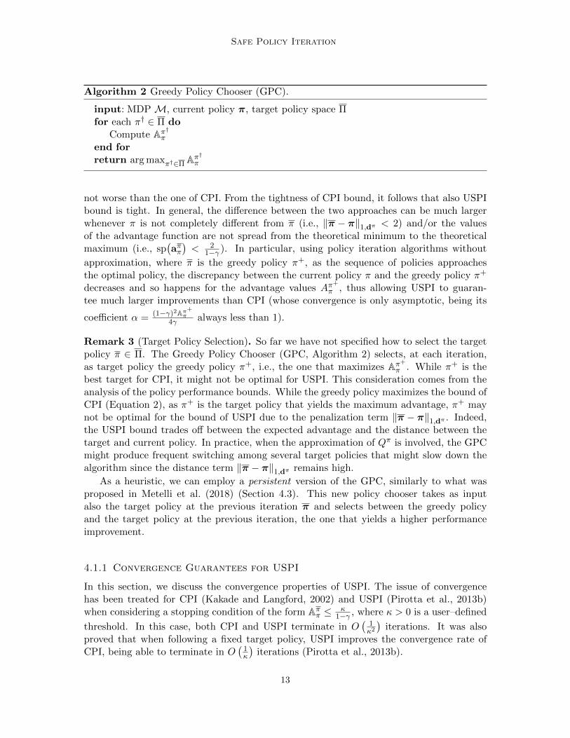
Algorithm 2 Greedy Policy Chooser (GPC).
input: MDP M, current policy π, target policy space Πfor each π† ∈ Π do
Compute Aπ†πend forreturn arg maxπ†∈Π Aπ†π
not worse than the one of CPI. From the tightness of CPI bound, it follows that also USPIbound is tight. In general, the difference between the two approaches can be much largerwhenever π is not completely different from π (i.e., ‖π − π‖1,dπ < 2) and/or the valuesof the advantage function are not spread from the theoretical minimum to the theoreticalmaximum (i.e., sp
(aππ)< 2
1−γ ). In particular, using policy iteration algorithms without
approximation, where π is the greedy policy π+, as the sequence of policies approachesthe optimal policy, the discrepancy between the current policy π and the greedy policy π+
decreases and so happens for the advantage values Aπ+
π , thus allowing USPI to guaran-tee much larger improvements than CPI (whose convergence is only asymptotic, being its
coefficient α = (1−γ)2Aπ+π4γ always less than 1).
Remark 3 (Target Policy Selection). So far we have not specified how to select the targetpolicy π ∈ Π. The Greedy Policy Chooser (GPC, Algorithm 2) selects, at each iteration,as target policy the greedy policy π+, i.e., the one that maximizes Aπ+
π . While π+ is thebest target for CPI, it might not be optimal for USPI. This consideration comes from theanalysis of the policy performance bounds. While the greedy policy maximizes the bound ofCPI (Equation 2), as π+ is the target policy that yields the maximum advantage, π+ maynot be optimal for the bound of USPI due to the penalization term ‖π − π‖1,dπ . Indeed,the USPI bound trades off between the expected advantage and the distance between thetarget and current policy. In practice, when the approximation of Qπ is involved, the GPCmight produce frequent switching among several target policies that might slow down thealgorithm since the distance term ‖π − π‖1,dπ remains high.
As a heuristic, we can employ a persistent version of the GPC, similarly to what wasproposed in Metelli et al. (2018) (Section 4.3). This new policy chooser takes as inputalso the target policy at the previous iteration π and selects between the greedy policyand the target policy at the previous iteration, the one that yields a higher performanceimprovement.
4.1.1 Convergence Guarantees for USPI
In this section, we discuss the convergence properties of USPI. The issue of convergencehas been treated for CPI (Kakade and Langford, 2002) and USPI (Pirotta et al., 2013b)when considering a stopping condition of the form Aππ ≤ κ
1−γ , where κ > 0 is a user–defined
threshold. In this case, both CPI and USPI terminate in O(
1κ2
)iterations. It was also
proved that when following a fixed target policy, USPI improves the convergence rate ofCPI, being able to terminate in O
(1κ
)iterations (Pirotta et al., 2013b).
13

Metelli, Pirotta, Calandriello, and Restelli
Our contribution to the convergence analysis consists in analyzing the case κ = 0, as inAlgorithm 1. Of course, in this case, the convergence guarantees of CPI are vacuous. Thissection is organized as follows. We start by proving that USPI (and CPI) converges asymp-totically under some assumptions on the γ–discounted state distribution (Assumption 1).Then, we show that, when the optimal policy is unique (Assumption 2), USPI convergesto the optimal policy in a finite number of iterations (Theorem 11). The proofs of all thepresented results are reported in Appendix A.2.
We start with the following lemma, which extends the Corollary 4.5 in Kakade andLangford (2002), and relates the expected advantage to the performance difference.
Lemma 7. Let π, π′ ∈ ΠSR be two arbitrary policies and π+ be a greedy policy induced byQπ. Then, the expected advantage Aπ+
π can be lower bounded as:
Aπ+
π
1− γ ≥∥∥∥∥∥dπ′
dπ
∥∥∥∥∥
−1
∞
(Jπ′ − Jπ
), (3)
where dπ′
dπ is the vector obtained by the element–wise division between dπ′
and dπ.
This result is very general since policy π′ is chosen arbitrarily. Clearly, the bound ismeaningful when Jπ
′> Jπ as we know that Aπ+
π ≥ 0. A straightforward choice of π′ is, ofcourse, a greedy policy π+. In this case, we are able to lower bound the expected advantagefunction Aπ+
π in terms of the performance gap itself:
Aπ+
π
1− γ ≥∥∥∥∥∥dπ
+
dπ
∥∥∥∥∥
−1
∞
(Jπ
+ − Jπ).
Remark 4 (On the γ–discounted stationary distribution). How can we ensure that
∥∥∥∥dπ′
dπ
∥∥∥∥∞<
+∞ is satisfied? A sufficient condition for
∥∥∥∥dπ′
dπ
∥∥∥∥∞< +∞ is that for any policy π and for
any state s, we have dπ(s) > 0. In particular, if the distribution of the initial state is positiveµ(s) > 0 for all states s ∈ S the condition is satisfied, indeed dπ = (1 − γ)µ + γPπTdπ ≥(1 − γ). When dπ(s) > 0 for every s and policy π, it admits for every state s a positiveminimum over the set of Markovian stationary policies. This is a consequence of the factthat dπ is a continuous function w.r.t. the policy π (Corollary 1 provides the Lipschitzcontinuity of dπ w.r.t. π) and the set of Markovian stationary policies ΠSR is compact.Moreover, if we consider finite state spaces dπ(s) admits a positive minimum also over thestate space, that we will denote with ∆d. Therefore, under this assumption, we can provide
the bound:
∥∥∥∥dπ′
dπ
∥∥∥∥∞≤ 1
∆d. From now on, we are going to make the following assumption.
Assumption 1. For all π ∈ ΠSR it holds that ∆d > 0, where ∆d = mins∈S {dπ(s)}.
Assumption 1 requires that each state is visited a (discounted) number of times at leastequal to ∆d > 0. A sufficient condition is that the initial state distribution µ visits withnon–zero probability each state of the MDP. In such case, ∆d ≥ (1− γ) mins∈S{µ(s)}.
14

Safe Policy Iteration
Theorem 8 (Convergence Bound). Under Assumption 1, USPI (and CPI) with GPC andtermination condition Aπ+
π ≤ 0 asymptotically converges to the optimal policy, i.e., let N > 0and πN be the policy visited by USPI (or CPI) at iteration N > 0, it holds that:
J∗ − JπN ≤ 8γ
N∆2d(1− γ)3
.
Proof Let us consider a step of USPI starting from policy πi and getting to policy πi+1.For Corollary 6, by noticing that ‖qπ‖∞ ≤ 1/(1 − γ) for any π ∈ ΠSR, the performanceimprovement is given by:
Jπi+1 − Jπi ≥(1− γ)
(Aπ
+iπi
)2
2γ∥∥π+
i − πi∥∥2
∞
≥(1− γ)
(Aπ
+iπi
)2
8γ, (P.7)
where π+i is a deterministic greedy policy. We now define the performance gap w.r.t. the
optimal policy ∆i = J∗ − Jπi . By changing the sign on both sides of Equation (P.7),summing J∗µ, and recalling the definition of ∆i we get the following inequality:
J∗ − Jπi+1 ≤ J∗ − Jπi −(1− γ)
(Aπ
+iπi
)2
8γ
∆i+1 ≤ ∆i −(1− γ)
(Aπ
+iπi
)2
8γ.
We now determine the convergence bound. Using Lemma 7 choosing π′ = π∗ we can lower
bound the expected advantage function Aπ+iπi and write:
∆i+1 ≤ ∆i −∥∥∥∥∥dπ
+i
dπi
∥∥∥∥∥
−2
∞
(1− γ)3.(∆i)2
8γ
Let us now consider the following expression:
1
∆i+1− 1
∆i=
∆i −∆i+1
∆i+1∆i≥ ∆i −∆i+1
∆2i
≥∥∥∥∥∥dπ
+i
dπi
∥∥∥∥∥
−2
∞
(1− γ)3
8γ,
where we simply exploited the monotonicity property of ∆i due to the guaranteed perfor-mance improvement. We can now sum over i and exploiting the telescopic property weget:
1
∆N≥ 1
∆0+
(1− γ)3
8γ
N−1∑
i=0
∥∥∥∥∥dπ
+i
dπi
∥∥∥∥∥
−2
∞
≥ N (1− γ)3
8γmin
i∈{0,1,...,N−1}
∥∥∥∥∥dπ
+i
dπi
∥∥∥∥∥
−2
∞
.
Solving for ∆N we have:
∆N = J∗ − JπN ≤ 8γ
N(1− γ)3max
i∈{0,1,...,N−1}
∥∥∥∥∥dπ
+i
dπi
∥∥∥∥∥
2
∞
≤ 8γ
N∆2d(1− γ)3
.
15
Metelli, Pirotta, Calandriello, and Restelli
Thus, USPI converges asymptotically with convergence bound of order O(N−1). Noticethat in the Equation (P.7) we upper-bounded the policy distance with 2 and thus, we con-sidered the same setting as CPI. As a consequence, this result applies as is to CPI.
Remark 5 (On the Convergence Bound). The convergence bound we derived in Theorem 8
has a polynomial dependence on the iteration number N , i.e., O(
1N(1−γ)3
). This appears
to be suboptimal compared to PI and VI both having a convergence bound that depends
exponentially on N , i.e., O(γN
1−γ
)(Puterman, 2014). In addition, also CPI with a constant
learning rate α ∈ [0, 1] achieves an exponential convergence O(
(1−α−γα)N
1−γ
)(Scherrer, 2014).
It is not surprising that these algorithms allow for a better convergence bound. Indeed, inthe exact setting, having access to the true greedy policy, we can safely perform a completeimprovement step, i.e., setting α = 1. CPI and SPI are meant to be employed in theapproximate setting (Section 5) when only an approximately greedy policy is available and,consequently, we cannot fully trust it.
We now prove that USPI converges to the optimal policy in a finite number of stepswhen using GPC. We outline the steps of the proof. First, we need to guarantee that aftera finite number of steps, USPI selects an optimal policy as target policy (Lemma 9). Thisfollows by observing that the performance difference between an optimal policy and thesecond-best deterministic policy is finite and by applying Theorem 8 to bound the numberof steps. Second, we need to ensure that when selecting an optimal policy as target, USPIconverges to it in a finite number of steps. This is the most delicate part of the proof, as thefinite convergence is a consequence of the interaction between the expected advantage Aπ∗πand the distance ‖π∗−π‖∞. It must happen that the distance decreases at least as fast asthe advantage when π → π∗ (Lemma 10). With GPC, this can be guaranteed only in thepresence of a unique (deterministic) optimal policy. Therefore, in the presence of multipleoptimal policies, switching between one and another might prevent finite convergence. Weare unable to guarantee that, in the presence of multiple optimal policies, GPC keepsselecting the same optimal policy; thus, we restrict our attention to the case in which theoptimal policy is unique. In the following, we denote with Π∗ for the set of optimal policies.
Lemma 9. Assume the same setting as Theorem 8. Let ∆J = J∗ −maxπ∈ΠSD\Π∗{Jπ} bethe performance gap between the optimal policies and the second-best deterministic policy,where Π∗ = {π ∈ ΠSD : Jπ = J∗}. Then, USPI (and CPI) with GPC selects an optimalpolicy as target policy after a finite number of iterations.
Clearly, once we select an optimal policy as target policy, we will never select a subpo-timal policy as target later as it could only decrease the performance. We can now provethat when following a deterministic optimal policy as target policy, the expected advantageAπ∗π can be lower bounded by a function of the distance ‖π∗ − π‖∞.
Lemma 10. Assume the same setting as Lemma 9. It π∗ is a deterministic optimal policy,then, there exists a constant ∆+ > 0 such that:
Aπ∗π ≥
∆d∆+
2‖π∗ − π‖∞ . (4)
16

Safe Policy Iteration
So far, we did not exploit the assumption on the uniqueness of the optimal policy. Inthe following theorem, the assumption is crucial.
Assumption 2. The optimal policy π∗ is unique.
Lemma 10 shows that, apart from constants, the expected advantage Aπ∗π decreasesat most as fast as the distance ‖π∗ − π‖∞. We can exploit this result, together withthe uniqueness of the optimal policy, to prove that USPI converges in a finite number ofiterations.
Theorem 11 (Finite Convergence). Under Assumption 1 and 2, USPI with GPC and ter-mination condition Aπ+
π ≤ 0 converges to the optimal policy in a finite number of iterations.
Proof First of all, we know from Lemma 9 that the algorithm will select the (unique)optimal policy π∗ as target policy after a finite number of iterations, say N1. Thus, fori > N1, we have that Jπi ≥ J∗ −∆J and moreover:
Jπi+1 − Jπi ≥(1− γ)
(Aπ∗πi
)2
2γ∥∥π∗ − πi
∥∥2
∞
≥(1− γ)∆2
d∆2+
∥∥π∗ − πi∥∥2
∞
8γ∥∥π∗ − πi
∥∥2
∞
=(1− γ)∆2
d∆2+
8γ,
where the first inequality is obtained from Equation (P.7) and the second inequality fromLemma 10. Since at each iteration the performance improves by a finite quantity, thealgorithm will need additional N2 iterations to fill the gap ∆J between the performance ofthe policy πN1 and the performance of the optimal policy π∗:
N2(1− γ)∆2
d∆2+
8γ≥ ∆J =⇒ N2 ≥
8γ∆J
∆2d∆
2+(1− γ)
.
Consequently, the algorithm will converge in N1 +N2 iterations.
4.2 per–State–parameter Safe Policy Improvement
The USPI approach aims at finding the convex combination between a starting policy πand a target policy π that maximizes the bound on the performance improvement (eitherTheorem 3 or Corollary 4). In this section, we consider a more general kind of update,where the new policy π′ is generated using different convex combination coefficients foreach state:
π′(a|s) = α(s)π(a|s) +(1− α(s)
)π(a|s), ∀s ∈ S, ∀a ∈ A, (5)
where α(s) ∈ [0, 1],∀s ∈ S. We name the resulting algorithm as per–State–parameter SafePolicy Iteration (SSPI).5 When per-state parameters are exploited, the bound in Theorem 3requires solving two dependent maximization problems over the state space that do notadmit a simple solution. Therefore, to compute the values α(s), we consider the simplifiedbound from Corollary 4. We can state the following result.
5. SSPI was called Multiple–parameter Safe Policy Improvement (MSPI) in Pirotta et al. (2013b). Thereason for the change of the name is due to the fact that we will present another approach exploitingmultiple parameters (Section 4.3).
17

Metelli, Pirotta, Calandriello, and Restelli
Corollary 12. Let Sππ be the subset of states where the advantage of policy π over policyπ and dπ are positive: Sππ = {s ∈ S : dπ(s)Aππ(s) > 0}. The bound in Corollary 4 is
optimized by taking α(s) = 0, ∀s /∈ Sππ and α(s) = min{
1, Υ ∗‖π(·|s)−π(·|s)‖1
}, ∀s ∈ Sππ , where
‖π(·|s)− π(·|s)‖1 =∑
a∈A |π(a|s)−π(a|s)| and Υ ∗ is the value that maximizes the followingfunction:
B(Υ ) =1
1− γ∑
s∈Sππ
min
{1,
Υ
‖π(·|s)− π(·|s)‖1
}dπ(s)Aππ(s)− Υ 2 γ
(1− γ)2
‖qπ‖∞2
.
Proof This proof starts from the transformation of several terms involved in Corollary 4exploiting the definition of π′ (see Equation 5). The average advantage Aππ can be statedas follows for all s ∈ S:
dπ(s)Aπ′π (s) = dπ(s)
∑
a∈A
(π′(a|s)− π(a|s)
)Qπ(s, a)
= dπ(s)∑
a∈Aα(s)
(π(a|s)− π(a|s)
)Qπ(s, a)
= α(s)dπ(s)Aππ(s).
Exploiting the definition of L∞–norm of a matrix, we can write:
∥∥π′ − π∥∥∞ = sup
s∈S
{∑
a∈A
∣∣∣π′(a|s)− π(a|s)∣∣∣}
= sups∈S{α(s) ‖π(·|s)− π(·|s)‖1} .
We can now restate the bound of Corollary 4 into the proposed framework:
Jπ′ − Jπ ≥ 1
1− γ∑
s∈Sα(s)dπ(s)Aππ(s)
− γ
(1− γ)2sups∈S{α(s) ‖π(·|s)− π(·|s)‖1}2
‖qπ‖∞2
.
(P.8)
The optimal values of α(s) do not admit a closed–form solution but can be computediteratively. Given a state s with negative advantage Aππ, the larger α(s) is, the lower will bethe bound on the policy improvement as expressed in Equation (P.8) (or in Corollary 4),so the optimal choice for these states is to set α(s) = 0. Similarly, if dπ(s) = 0, state s doesnot have any contribution to the bound, so we can set α(s) = 0.
Given these conditions, we define Sππ = {s ∈ S : dπ(s)Aππ(s) > 0}. Then, Υ denotes theL∞–norm of the difference of the policies over Sππ :
Υ = sups∈Sππ
{α(s) ‖π(·|s)− π(·|s)‖1} ,
we can now introduce the following condition:
α(s) ‖π(·|s)− π(·|s)‖1 ≤ Υ, ∀s ∈ Sππ . (P.9)
18

Safe Policy Iteration
Algorithm 3 Exact SSPI.
input: MDP M, target policy space Π, policy chooser PCInitialize ππ ← PC(M,Π, π)Υ ∗ ← FBO(M, π, π) (see Alg. 4)while Υ ∗ > 0 do
α(s)← min{
1, Υ∗
‖π(·|s)−π(·|s)‖1
}, ∀s ∈ S
π(a|s)← α(s)π(a|s) + (1− α(s))π(a|s), ∀s ∈ S, ∀a ∈ Aπ ← PC(M,Π, π)Υ ∗ ← FBO(M, π, π)
end while
If we suppose to fix Υ , the previous relationship and the knowledge of α ∈ [0, 1] impose thefollowing equivalence:
α(s) = min
{1,
Υ
‖π(·|s)− π(·|s)‖1
}, ∀s ∈ Sππ .
Consider Equation (P.8), once the supremum is fixed, we cannot do better than set the othercoefficients α(s) to the maximum feasible value that does not make α(s) ‖π(·|s)− π(·|s)‖1exceed the supremum. As mentioned before, states with negative advantage play as oppo-nents, their influence is minimized by putting α(s) = 0 in correspondence of such states.
Function B(Υ ) is obtained by manipulating the bound (P.8) using these considerations.As a result, the optimization of the bound over the set of |S| coefficients α(s) has beentranslated into the maximization of the univariate function B(Υ ). However, since the supe-rior Υ is not known a priori, an iterative approach has to be carried out. Once the optimalvalue Υ ∗ is obtained, the following rule can be applied:
α(s) =
{min
{1, Υ ∗‖π(·|s)−π(·|s)‖1
}∀s ∈ Sππ
0 otherwise.
The pseudocode of SSPI is reported in Algorithm 3. The algorithm stops as the optimalbudget Υ ∗ becomes zero, i.e., when in all states the advantage Aππ(s) ≤ 0.
4.2.1 Computing Υ ∗
Differently from USPI, the coefficients of SSPI cannot be computed in closed form due totheir dependency from Υ ∗, whose value requires the maximization of a function with discon-tinuous derivative (Corollary 12). This search formalizes the trade-off between increasingthe probability budget Υ , and incur in a larger penalty while obtaining a gain by movingfurther towards the target policy. In order to solve this problem, we consider the graph inFigure 1, where we can see that function B is a continuous quadratic piecewise function,whose derivative is a discontinuous linear piecewise function. It is important to underline
that all the pieces of the partial derivative of B have the same slope m = −γ‖qπ‖∞(1−γ)2
. Suppose
19

Metelli, Pirotta, Calandriello, and Restelli
0.23 0.4 1.03 1.25 1.49 1.82−0.2
−0.1
0
0.1
Υ1 Υ2 Υ3 Υ4 Υ5 Υ6Υ ∗
−0.4
−0.2
0
0.2
Υ
Magn
itudeofthebound
g0
Magnitudeofthegradient
B∂B/∂Υ
(a)
0.23 0.4 1.03 1.25 1.49 1.82−5 · 10−2
0
5 · 10−2
0.1
0.15
0.2Υ1 Υ2 Υ3Υ4 Υ5 Υ6Υ ∗
0
0.2
0.4
Υ
Magnitudeof
thebou
nd
g0
Magnitudeof
thegrad
ient
B∂B/∂Υ
(b)
Figure 1: Bound B and its derivative. Blue–filled circles are set in correspondence withthe discontinuities, whereas the blue triangle represents the maximum value ofB. The gradient of B is depicted by the dashed brown piecewise linear functionwhere the red square represents g0, its evaluation in Υ = 0.
20

Safe Policy Iteration
Algorithm 4 Computing Υ ∗ (Forward Bound Optimizer - FBO)
input: MDP M, current policy π, target policy π
initialize: i← 1, m← −γ‖qπ‖∞
(1−γ)2 Υ0, q0 ← FJP(M, π, π), g0 ← q0
while Υi < 2 doΥi, qi ← FJP(M, π, π) (see Alg. 5)gi ← gi−1 +m · (Υi − Υi−1)if gi ≤ 0 then
return Υi − gim
end ifgi ← gi − qi−1 + qiif gi ≤ 0 then
return Υiend ifi← i+ 1
end whilereturn Υi
we are given a function FJP (Find Jump Point) that returns the coordinates (Υ, q) of thenext discontinuity point of the derivative of B. Then, the maximization of B can be com-puted using an iterative algorithm like the one proposed in Algorithm 4, Forward BoundOptimizer (FBO).6 The idea is to start from Υ = 0 and to search for the zero–crossingvalue of the derivative of B by running over the discontinuity points. The algorithm stopswhen either the derivative of B becomes negative or when we reach the maximum value ofΥ , i.e., Υ = 2 (the last return in Algorithm 4). When the derivative becomes negative, twodifferent cases may happen: (i) the derivative equals zero at some value of Υ (as it happensin Figure 1a), which is the case of the first return in Algorithm 4; (ii) the derivative becomesnegative in correspondence of a discontinuity without taking the value of zero (the secondreturn in Algorithm 4), i.e., the maximum falls on an angular point of B (see Figure 1b).Notice that, as we presented it, Algorithm 4 can be used to optimize any function withlinear piecewise derivative, provided that all pieces have the same slope.
Clearly, we need to be able to determine the discontinuity points of the derivative, i.e.,we need to specify function FJP. For this purpose, we write down explicitly the derivative:
∂
∂ΥB(Υ ) =
1
1− γ∑
s∈SΥ
dπ(s)Aππ(s)
‖π(·|s)− π(·|s)‖1− Υ γ ‖q
π‖∞(1− γ)2
= g(Υ ) +mΥ, (6)
where SΥ ={s ∈ Sππ : ‖π(·|s)− π(·|s)‖1 > Υ
}is the set of all the states in which the
coefficient α(s) is dependent on Υ . Since the derivative is non-negative at Υ = 0, and itis monotonically decreasing, B is guaranteed to have a unique maximum. The disconti-nuity points correspond to values of Υ for which some state s saturates its coefficient to1, so that, for larger values Υ , the coefficient α(s) does not depend on Υ anymore, thusdisappearing from the derivative whose value changes discontinuously with a jump equal to
dπ(s)Aππ(s)(1−γ)‖π(·|s)−π(·|s)‖1
. The procedure for finding the discontinuity points (FJP) is formalized
in Algorithm 5.
6. Differently from Pirotta et al. (2013b), we decided to keep the optimization of the bound (FBO) and theidentification of the discontinuity points (FJP) separated so that we can reuse FBO in Section 4.3.
21

Metelli, Pirotta, Calandriello, and Restelli
Algorithm 5 Computing of the jump points for SSPI (Find Jump Point - FJP)
input: MDP M, current policy π, target policy π
initialize: t← 0, Sππ ← {s ∈ S : dπ(s)Aππ(s) > 0}, Υ0 ← 0, q0 ← 11−γ
∑s∈Sππ
dπ(s)Aππ(s)‖π(·|s)−π(·|s)‖1
Sort states in Sππ so that i < j =⇒ ‖π(·|si)− π(·|si)‖1 ≤ ‖π(·|sj)− π(·|sj)‖1yield Υ0, q0
while Sππ 6= {} dot← t+ 1Υt ← ‖π(·|st)− π(·|st)‖1qt ← qt−1 − dπ(st)A
ππ(st)
(1−γ)‖π(·|st)−π(·|st)‖1Sππ ← Sππ \ {st}yield Υt, qt
end whileyield 2, −∞
The computational complexity of FJP is dominated by the cost of computing the L1-norm between the policies and the cost of sorting the states according to the discrepancybetween the current policy π and the target policy π, that is O (|S||A|+ |S| log |S|).Remark 6 (On the policy space of SSPI). When using per–state coefficients α(s) the spaceof policies accessible, by combining the target policies Π, is larger than that obtainable witha single coefficient α. Clearly, it is possible to enhance Π with additional policies so thateven USPI, with a unique coefficient α, can represent the same policies as SSPI. However,this transformation would produce, in the worst case, exponential growth in the number oftarget policies. Consider, for instance, the set of target policies Π = {πi(s) = ai : ∀s ∈S, i ∈ {1, ..., |A|}}. Thus, Π contains all the deterministic policies that perform the sameaction in all states. Consequently, |Π| = |A|. Using per–state coefficients α(s), we are ableto represent all Markovian randomized policies ΠSR. Those are the policies accessible bySSPI. Instead, starting with Π, USPI can represent just a subset of those. For USPI torepresent all Markovian randomized policies, we need to consider as target policy spacethe set of all Markovian deterministic policies ΠSD, whose cardinality is |A||S|. We cangeneralize the rationale to all the target policy spaces made up of deterministic policies.Let AΠ(s) = {a ∈ A : ∃π ∈ Π, π(s) = a} be the set of all actions that are prescribed instate s by the policies in Π. The transformation of the policy space is obtained as follows:
Π ={π(s) = a : ∀a ∈ AΠ(s), ∀s ∈ S
}(7)
It is worth noting that the cardinality of Π is given by∏s∈S |AΠ(s)| ≤ |A||S|.
Remark 7 (Comparing USPI and SSPI). Although SSPI maximizes over a set of policiesthat is a very large superset of the policies considered by USPI, it may happen that thepolicy improvement bound found by SSPI is smaller than the one of USPI. The reasonis that the former optimizes the bound in Corollary 4 that is looser than the bound inTheorem 3 optimized by the latter. Finally, notice that, following the same proceduredescribed in Remark 4 and constraining SSPI to use a single α for all the states (so that
the SSPI improvement is bounded by Aππ2
2γ‖π−π‖2∞‖qπ‖∞), we can prove, as done with USPI,
that the improvement of SSPI is never worse than the one of CPI.
22

Safe Policy Iteration
4.3 per–State–Action–parameter Safe Policy Improvement
We can further generalize SSPI by considering an update scheme in which the new policyis generated using different convex combination coefficients for each state–action pair:
π′(a|s) = α(s, a)π(a|s) +(1− α(s, a)
)π(a|s), (8)
where α(s, a) ∈ [0, 1], ∀s ∈ S, ∀a ∈ A. Note that, in order to ensure a valid probabilitydistribution we need to impose that, ∀s ∈ S,
∑a∈A α(s, a) (π(a|s)− π(a|s)) = 0. As for
SSPI, the bound in Theorem 3 cannot be optimized easily, thus we consider again thesimplified bound in Corollary 4.
The novel idea of this improvement scheme called per–State–Action–parameter Safe Pol-icy Improvement (SASPI), consists in the fact that, for each state, we can move probabilityacross the actions. For a given state s and action a, we define the probability increment in-duced by coefficient α(s, a) as ∆(s, a) = π′(a|s)−π(a|s) = α(s, a) (π(a|s)− π(a|s)). Clearly,we cannot change the probability arbitrarily, as we need to satisfy the following constraints:
∀s ∈ S,∑
a∈A∆(s, a) = 0, (9)
∀(s, a) ∈ S ×A,{
0 ≤ ∆(s, a) ≤ π(a|s)− π(a|s) if π(a|s) ≥ π(a|s)π(a|s)− π(a|s) ≤ ∆(s, a) ≤ 0 otherwise
. (10)
The constraint (9) ensures that the resulting policy π′(a|s) = π(a|s) + ∆(s, a) is a validprobability distribution for all s ∈ S, while constraint (10) guarantees that the chosen∆(s, a) realizes a convex combination of the entries of the current policy π and those of thetarget policy π. As a consequence, for each state s ∈ S we can partition the actions into threesets according to the sign of π(a|s)−π(a|s). A↑s = {a ∈ A : π(a|s) > π(a|s)} is the set of the
actions whose probability can only be increased, A↓s = {a ∈ A : π(a|s) < π(a|s)} is the set ofthe actions whose probability can only be decreased, and if A=
s = {a ∈ A : π(a|s) = π(a|s)}is the set of the actions whose probability cannot change whatever α(s, a) we pick.
To solve the problem of determining the optimal values of the ∆(s, a), we adopt anapproach similar to that of SSPI and we introduce a budget Υ = ‖π′ − π‖∞, with π′ asdefined in Equation (8). Notice that Υ can be spent independently in each state s, bydefinition of L∞-norm. Suppose we are able to find the optimal budget value Υ ∗, ouroptimization problem consists of maximizing the bound in Corollary 4 over the probabilityincrements ∆(s, a) having a fixed budget Υ and fulfilling the constraints (9) and (10).Ideally, we would like to increase the probability of the actions with high Qπ and decreasethe probability of the actions with low Qπ. Notice that, in order to satisfy (9), for each state,the amount of probability we add must coincide with the amount of probability we subtractacross all actions. Thus, given a budget Υ we can increase (resp. decrease) the probabilityof the actions by Υ/2 at most. In order to define the update rule, let ρπs : A → {1, 2, . . . , |A|}be an ordering of the actions for each state, such that if ρπs (a) < ρπs (a′) =⇒ Qπ(s, a) ≤Qπ(s, a′). We define the following quantities:
G↑(s, a) =∑
a′∈A↑s :ρπs (a′)>ρπs (a)
(π(a′|s)− π(a′|s)
),
23

Metelli, Pirotta, Calandriello, and Restelli
G↓(s, a) =∑
a′∈A↓s :ρπs (a′)<ρπs (a)
(π(a′|s)− π(a′|s)
).
Given an action a ∈ A, G↑(s, a) represents the amount by which the total probability ofall the actions with Qπ larger than Qπ(s, a) can be increased. Symmetrically, for an actiona ∈ A, G↓(s, a) represents the amount by which the total probability of all the actions withQπ smaller than Qπ(s, a) can be decreased. Note that it is not always convenient to spend Υcompletely in every state. Indeed, it might be the case that in order to spend it all, we haveto increase the probability of actions with low Qπ and decrease the probability of actionswith high Qπ, which is clearly inconvenient. For this reason, we define the expendable budgetfor an action a ∈ A in a state s ∈ S as:
Υ (s, a) =
max{
0,min{π(a|s)− π(a|s), G↓(s, a)−G↑(s, a)
}}if a ∈ A↑s
max{
0,min{π(a|s)− π(a|s), G↑(s, a)−G↓(s, a)
}}if a ∈ A↓s
0 otherwise
. (11)
To grasp the intuition behind the definition of expendable budget, consider an action a ∈ A↑s.We have two conditions to satisfy in order to define the budget Υ (s, a). First, for a we canincrease its probability by at most π(a|s)− π(a|s). However, this might not be convenientdepending on how much the probability of actions with Qπ smaller than Qπ(s, a) can bedecreased, i.e., G↓(s, a). The best way of moving probability across actions consists ofincreasing the probability of actions in decreasing order of Qπ and decreasing the probabilityof actions in increasing order of Qπ. Thus, the second condition can be stated as follows.Given an action a ∈ A↑s, recalling that we have increased the probability of all actions withQπ higher than Qπ(s, a) as much as possible, i.e., by G↑(s, a), the budget we have at ourdisposal is at most G↓(s, a) − G↑(s, a). Therefore, to define Υ (s, a) we take the minimumbetween the two cases, which leads to Equation (11). A similar rationale holds for actions
in A↓s. Clearly, for actions a ∈ A=s we have Υ (s, a) = 0. We can also define the expendable
budget for a state s ∈ S as: Υ (s) =∑
a∈A Υ (s, a). If Υ ≤ Υ (s) we can define the two
active actions, i.e., those of which we are currently increasing (a↑s) and decreasing (a↓s) theprobability:
a↑s = arg maxa∈A↑s :
G↑(s,a)≤Υ2
{ρπs (a)} , a↓s = arg maxa∈A↓s :
G↓(s,a)≤Υ2
{ρπs (a)} . (12)
We can now state the following optimality condition.
Corollary 13. Let Sππ = {s ∈ S : dπ(s) > 0} and Υ ∗ be the value that maximizes thefollowing function:
B(Υ ) =1
1− γ∑
s∈Sππ
dπ(s)∑
a∈A∆(s, a, Υ )Qπ(s, a)− γ
(1− γ)2Υ 2 ‖qπ‖∞
2,
where
∆(s, a, Υ ) =
max{
0,min{Υ (s, a), Υ2 −G↑(s, a)
}}if a ∈ A↑s
−max{
0,min{Υ (s, a), Υ2 −G↓(s, a)
}}if a ∈ A↓s
0 if a ∈ A=s
.
24

Safe Policy Iteration
We set ∆(s, a, Υ ) = 0 when dπ(s) = 0. Then, the bound in Corollary 4 is optimized bytaking
α(s, a) =
{0 if π(a|s) = π(a|s)
∆(s,a,Υ ∗)π(a|s)−π(a|s) otherwise
Proof First note that if dπ(s) = 0, state s does not have any contribution in the boundvalue, thus we can set ∆(s, a) = 0 and restrict our analysis to the states in Sππ . We nowevaluate the contribution of each action to the bound in Corollary 4:
Jπ′ − Jπ ≥ 1
1− γdπTaπ
′π −
γ
(1− γ)2
∥∥π′ − π∥∥2
∞‖qπ‖∞
2
=1
1− γ∑
s∈Sππ
dπ(s)∑
a∈A
[π′(a|s)Qπ(s, a)− π(a|s)Qπ(s, a)
]− γ
(1− γ)2
∥∥π′ − π∥∥2
∞‖qπ‖∞
2
=1
1− γ∑
s∈Sππ
dπ(s)∑
a∈A∆(s, a)Qπ(s, a)− γ
(1− γ)2Υ 2 ‖qπ‖∞
2,
where we denoted with ∆(s, a) = π′(a|s) − π(a|s) and Υ 2 = ‖π′ − π‖2∞. Consider a fixedbudget Υ . Since we can spend Υ independently in each state, we can reason for a genericstate s ∈ S. In particular, Υ/2 can be used to increase the probability of some actions in
A↑s and Υ/2 to decrease the probability of some actions in A↓s. The best we can do is tostart increasing the probabilities of actions starting from the one with the highest Qπ valueand, at the same time, decreasing the probabilities of actions starting from the one withthe lowest Qπ value, until we ran out of budget. Thus, for an action a ∈ A↑s we increase itsprobability as much as possible, i.e., by Υ (s, a). But we need to limit the increment if wedo not have enough budget. Thus, if Υ (s, a) > Υ/2 − G↑(s, a) we need to set the increaseto zero. Summing up, we have:
∆(s, a) = max
{0,min
{Υ (s, a),
Υ
2−G↑(s, a)
}}, ∀s ∈ S,∀a ∈ A↑s. (P.10)
Analogously, for all actions a ∈ A↓s we decrease the probability as much as possible, providedthat we have enough budget:
∆(s, a) = −max
{0,min
{Υ (s, a),
Υ
2−G↓(s, a)
}}, ∀s ∈ S, ∀a ∈ A↓s. (P.11)
For the actions a ∈ A=s we need to set ∆(s, a) = 0. Recalling that α(s, a) = ∆(s,a)
π(a|s)−π(a|s) weget the result.
Algorithm 6 provides the pseudocode of SASPI. Similarly to SSPI, the terminationcondition is Υ ∗ = 0, i.e., when no improvement can be obtained with the target policy π.
4.3.1 Computing Υ ∗
Like for SASPI, we face the problem of computing Υ ∗, which requires the maximization ofa function with linear discontinuous derivative. Note that, once again, the slope of each
25

Metelli, Pirotta, Calandriello, and Restelli
Algorithm 6 Exact SASPI.
input: MDP M, target policy space Π, policy chooser PCInitialize ππ ← PC(M,Π, π)Υ ∗ ← FBO(M, π, π) (see Alg. 4)while Υ ∗ > 0 do
Compute Υ (s, a), ∀s ∈ S, ∀a ∈ A
∆(s, a)←
max{
0,min{Υ (s, a), Υ2 −G↑(s, a)
}}if a ∈ A↑s,
−max{
0,min{Υ (s, a), Υ2 −G↓(s, a)
}}if a ∈ A↓s,
0 if a ∈ A=s ,
∀s ∈ S,∀a ∈ A
α(s, a)← ∆(s,a)π(a|s)−π(a|s) ∀s ∈ S,∀a ∈ A
π(a|s)← α(s, a)π(a|s) + (1− α(s, a))π(a|s), ∀s ∈ S, ∀a ∈ Aπ ← PC(M,Π, π)Υ ∗ ← FBO(M, π, π)
end while
piece is the same and equal to m = −γ‖q‖∞(1−γ)2
. For this reason, provided that we are able
to compute the coordinates of the discontinuity points (by using a properly defined FJP),we can employ Algorithm 4 to find Υ ∗. Let us now write the explicit expression of thederivative of the bound:
∂
∂ΥB(Υ ) =
1
1− γ∑
s∈SΥ
1
2dπ(s)
(Qπ(s, a↑s)−Qπ(s, a↓s)
)− Υ γ ‖q
π‖∞(1− γ)2
= g(Υ ) +mΥ, (13)
where SΥ = {s ∈ S : Υ (s) ≤ Υ} is the set of states for which we still have budget (non-saturated) and thus their contribution in the summation is dependent on Υ . In such a case,
there exist two active actions, as defined in Equation (12): a↑s of which we are increasing the
probability and a↓s of which we are decreasing the probability. The probability of the otheractions are either saturated to the maximum value or kept unchanged and thus, independentof Υ . Similarly to what happens in SSPI, the derivative is non negative at Υ = 0, and itis monotonically decreasing since both Qπ(s, a↑s) and −Qπ(s, a↓s) are decreasing functions
of Υ . Therefore, B is guaranteed to have a unique maximum since actions a↑s and a↓s areconsidered in decreasing and increasing order of Qπ, respectively. The discontinuity pointscorrespond to values of Υ for which either one state saturates, i.e., Υ reaches Υ (s), or a↑sor a↓s change. In order to find these discontinuity points, we can adopt Algorithm 7. Theidea of the algorithm is to go through state–action pairs sorted according to the budgetat which they are going to saturate. This information is provided by G↑(s, a) for actionscandidate to increase their probability and by G↓(s, a) for actions candidate to decrease theirprobability. Therefore we consider two orderings ρ↑ and ρ↓ in which the state–action pairsare sorted according to G↑(s, a) and G↓(s, a), respectively. At each iteration t we considerthe pair (s, a) that will saturate sooner (the first if). For this pair, two situations mighthappen: (i) it is convenient to perform the update, i.e., the action at whose probabilityis going to be increased (resp. decreased) has higher Qπ than the action we have just
decreased (resp. increased) the probability a↓st ; (ii) the update is not convenient. In case(ii), we need to declare the state st as saturated and remove it from the set Sππ . The
26

Safe Policy Iteration
-1.369 -0.058 0.783 1.201 1.8820
0.2
0.4
0.6
0.8
a1 a2 a3 a4 a5
0
10.5
0
0.8
ρπs
Υ = 0.4 Υ(s) = 0.4
Qπ
π(ai|s)π(a|s)π′(a|s)π(a|s)
-1.369 -0.058 0.783 1.201 1.8820
0.2
0.4
0.6
0.8
a1 a2 a3 a4 a5
01
0
0
1
ρπs
Υ = 0.4 Υ(s) = 0.2
Qπ
π(ai|s)π(a|s)π′(a|s)π(a|s)
Figure 2: SASPI policy update.
computational complexity of Algorithm 7 is dominated by the computation of the orderingsρ↑ and ρ↓, which costs O (|S||A| log |A||S|), as the computation of G↑(s, a) and G↓(s, a) hascost O (|S||A| log |A|) and the loop is executed at most |S||A| times and at each iterationthe cost is constant. In the following, we report a couple of examples of policy update usingSASPI.
Example 1. The initial policy (blue area with dotted mark), the updated policy (orangearea with square mark) and the target policy (green area with diamond mark) are depictedin Figure 2. Actions are ordered according to ρπs , i.e., in ascending order according to theirQ–values. We fix a budget Υ = 0.4. At the top, we show a case in which we are able tospend the whole budget in state s, i.e., Υ (s) = 0.4. We start from the best a5 and the worsta1 actions. We try to increase the probability of a5 and decrease that of a1, but we cannotas π(a1|s) > π(a1|s), so we move to action a2. We decrease the probability of a2 by 0.1 andwe increase the probability of a5 by the same amount. Now, we move to action a3 and wedecrease its probability by 0.1 as well while increasing that of a5 by the same amount. Sincewe have no further budget, we stop. At the bottom, we show a case where the expendablebudget Υ (s) = 0.2 is less than Υ . Again we start with a1 and a5. Similar to the case on theleft, we have to move to a2. Now, we can increase the probability of a5 by 0.1 and meanwhilereduce the probability of a2 by the same amount. We could now decrease the probability ofa3 but we have not enough probability on a4 to compensate. Thus, we stop. The updates∆(s, a) are reported in the figure as dashed arrows. Coefficients α(s, ai) are drawn abovethe bars.
Remark 8 (SASPI vs SSPI). It is worth noting that the more flexible update rule intro-duced by SASPI shows an advantage over SSPI only when considering problems with morethan two actions. Indeed, when A = {a1, a2} we have that α(s, a1) = α(s, a2) since fromConstraint (9) we have:
0 = ∆(s, a1) + ∆(s, a2) = α(s, a1) (π(a1|s)− π(a1|s)) + α(s, a2) (π(a2|s)− π(a2|s))
27

Metelli, Pirotta, Calandriello, and Restelli
Algorithm 7 Computing of the jump points for SASPI (Find Jump Point - FJP)
input: MDP M, current policy π, target policy πinitialize: t← 0, Sππ ← {s ∈ S : dπ(s) > 0}, Υ0
2 ← 0, i↑ ← 0, i↓ ← 0Compute G↑(s, a) and G↓(s, a), ∀s ∈ S, ∀a ∈ ACompute the two orderings ρ↑ and ρ↓ such that s.t. i < j =⇒ G↑(sρ↑i
, aρ↑i) ≤ G↑(sρ↑j
, aρ↑j) and
i < j =⇒ G↓(sρ↓i, aρ↓i
) ≤ G↑(sρ↓j , aρ↓j )
Compute a↑s = arg maxa∈A {Qπ(s, a)} and a↓s = arg mina∈A {Qπ(s, a)}, ∀s ∈ Sq0 ← 1
1−γ∑s∈Sππ
12dπ(s)
(Qπ(s, a↑s)−Qπ(s, a↓s)
)
yield Υ0, q0
while Sππ 6= {} dot← t+ 1if st ∈ Sππ then
if G↑(sρ↑,i↑aρ↑
i↑) ≤ G↓(sρ↓
i↓, aρ↓
i↓) then
st, at ← sρ↑i↑, aρ↑
i↑
if Qπ(st, at) > Qπ(st, a↓st) then
qt ← qt−1 − 12dπ(st)
(Qπ(st, a
↑sit)−Qπ(st, at)
)
a↑st ← atelse
qt ← qt−1 − 12dπ(st)
(Qπ(st, a
↑st)−Qπ(st, a
↓st))
Sππ \ {st}end ifΥt2 ← G↑(st, at)i↑ ← i↑ + 1
elsest, at ← sρ↓
i↓, aρ↓
i↓
if Qπ(st, at) < Qπ(st, a↓st) then
qt ← qt−1 − 12dπ(st)
(Qπ(st, at)−Qπ(st, a
↓st))
a↓st ← atelse
qt ← qt−1 − 12dπ(st)
(Qπ(st, a
↑st)−Qπ(st, a
↓st))
Sππ \ {st}end ifΥt2 ← G↓(st, at)i↓ ← i↓ + 1
end ifend ifyield Υt, qt
end whileyield 2, −∞
= (α(s, a1)− α(s, a2)) (π(a1|s)− π(a1|s)) =⇒ α(s, a1) = α(s, a2).
As a consequence, the coefficient α depends on the state only, like in SSPI.
Remark 9 (Optimality of USPI, SSPI and SASPI). In general, selecting a greedy policyπ+ as target policy for USPI and SSPI is not optimal in terms of bound value, i.e., theremight exist a target policy π 6= π+ that allows reaching higher values of the bound. Indeed,
28

Safe Policy Iteration
as proved in Appendix B, the policy that maximizes globally the bound, as defined inCorollary 29, might be outside the space of representable policies given the USPI and SSPIupdate rule. On the contrary, this policy is always representable with the update rule ofSASPI provided that we select π+ as target policy. Thus, SASPI is optimal in terms ofbound value using the GPC (Greedy Policy Chooser, Algorithm 2).
Remark 10 (On the Convergence of SSPI and SASPI). We have not provided a specific re-sult for the convergence of SSPI and SASPI. It is worth noting that these two algorithms con-verge to the optimal policy under the same assumptions enforced for USPI (Section 4.1.1).Indeed, the convergence proof (Theorem 8) employs the performance improvement pro-duced by USPI as in Corollary 6, i.e., USPI with the simplified bound. SSPI and SASPIyield a larger policy improvement compared to that of Corollary 6 and, consequently, theschema of the proof applies straightforwardly.
5. Approximate Safe Policy Iteration
The exact algorithms proposed in the previous sections are impractical in applications wherethe state space is very large (or even continuous) or when the state–transition model isunknown. In this section, we move to the approximate setting in which the quantitiesinvolved in the bounds need to be estimated from samples. We start introducing theapproximate versions of the policy choosers (Section 5.1), then we present the approximateversions of the three algorithms we introduced in Section 4: aUSPI (Section 5.2), aSSPI(Section 5.3), and aSASPI (Section 5.4). For each of them, we present the algorithm, asample complexity analysis and, when possible, we discuss the convergence properties.
Since accurate estimates of L∞–norms (sp(a) for USPI and ‖qπ‖∞ for SSPI, and SASPI)need many samples, for approximate settings, we consider a further simplified bound ob-tained from Corollary 4 by observing that ‖qπ‖∞ ≤ 1
1−γ :
Jπ′ − Jπ ≥ 1
1− γAπ′π −
γ
2(1− γ)3
∥∥π′ − π∥∥2
∞ . (14)
In this way, the only value that needs to be estimated is Aπ′π . Following Kakade (2003),the goal of this section is to provide an analysis of the SPI algorithms presented whendealing with tabular domains.
In the following, we will denote with the “hat” the estimated/approximated quantities.We will employ this notation for both the value functions (e.g., Qπ, Aππ) and the policies(e.g., π). Approximation involves essentially two parts of the SPI algorithms. First, thepolicy chooser needs samples to select in an approximate manner a suitable target policy.We will discuss in Section 5.1 how to extend the Greedy Policy Chooser (GPC) to accountfor samples. Second, once a target policy is available, we need to perform the policy updatecomputing the convex combination coefficients α. This latter phase heavily depends onthe SPI algorithm and we will discuss how to perform it for a fixed target policy in theSections 5.2–5.4. The proofs of all the presented results are reported in Appendix A.3.
29

Metelli, Pirotta, Calandriello, and Restelli
Algorithm 8 Approximate Greedy Policy Chooser (GPC).
input: current policy π, target policy space Π
initialize: N ←⌈
32|A|29ε2
(log(2|Π|) + log 1
δ
) ⌉, T ←
⌈logγ
ε24
⌉
Compute a biased sample set {(si, ai, qi)}Ni=1.for each π† ∈ Π do
Construct the estimate Qπ†
π = |A|N
∑Ni=1 q
πi π†(ai|si)
end for
return arg maxπ†∈Π
{Qπ†
π
}
5.1 Approximate Policy Choosers
Since we are in model–free setting, we need a new policy chooser that, at each iteration,given a policy π, returns the target policy π ∈ Π selected using samples. We will discuss inthis section how to adapt the Greedy Policy Chooser (GPC) to the approximate framework.
Let us first focus on the requirements for a generic approximate policy chooser PC, whichoutputs a target policy π. Given an accuracy level ε > 0 and an (exact) policy chooser
PC, the goal of the corresponding approximate policy chooser PC consists in returning anapproximate target policy π such that with probability at least 1 − δ, we have that thedifference between the expected advantage Aππ of the true target policy π and the expected
advantage Aππ of the approximate target policy π is bounded:∣∣∣Aππ − Aππ
∣∣∣ ≤ ε
1− γ , (15)
where π is the target policy returned by the exact policy chooser PC. Note that equivalentlywe can write that
π ∈ arg maxπ†∈Π
Aπ†π ,
where Aππ is the estimated expected advantage function of a candidate target policy π†.Considering the GPC, it is worth noting that the requirement at Equation (15) is notdissimilar from the typical requirement employed in API, i.e., the fact that the improvementstep is made by using an approximately greedy policy (Scherrer, 2014). Indeed, we can
rewrite the difference of the expected advantages as Aππ − Aππ = dπT(π − π
)qπ. Similar
conditions on the approximate greedy policy can be found in some fundamental works onAPI (e.g., Lagoudakis and Parr, 2003a; Lazaric et al., 2016). The pseudocode of approximate
GPC (GPC) is reported in Algorithm 8. The following lemma provides a sufficient conditionto meet the previous requirement.
Lemma 14. If with probability at least 1− δ, simultaneously for all π† ∈ Π it holds that:∣∣∣Qπ†
π −Qπ†π
∣∣∣ ≤ ε
2(1− γ), (16)
where Qπ†π = dπTπ†qπ, then with probability at least 1− δ it holds that:
∣∣∣Aππ − Aππ∣∣∣ ≤ ε
1− γ ,
30

Safe Policy Iteration
where π is the target policy returned by GPC and π is the policy returned by GPC (Algo-rithm 8).
Proof Let us denote with π the policy returned by GPC and with π the policy returnedby GPC. We consider the following sequence of inequalities:
Aππ − Aππ = Aππ − Aππ + Aππ − Aππ≤ Aππ − Aππ + Aππ − Aππ≤ 2 max
π†∈Π
{∣∣∣Aπ†π − Aπ†π
∣∣∣},
where we exploited the fact that Aππ ≤ Aππ, as GPC returns the policy π that maximizes
Aππ. We now observe that for any π† ∈ Π, Aπ†π = Qπ†π − Qπ
π. The result then follows fromthe hypothesis.
Thus, the problem translates into computing an ε2(1−γ)–accurate estimation of Qπ†
π for
all π† ∈ Π. To this purpose, we present the following sampling procedure.GPC Sampling Procedure The policy chooser generates a dataset {(si, ai, qi)}Ni=1 that for
each state-action pair (si, ai) reports an estimation of the Q-function of policy π, denoted byqi. The state si must be extracted according to the γ–discounted future state distributiondπ. In order to generate a sample si from dπ, we draw a state s0 from µ and then we followthe policy π. Since γ represents the probability of continuing the simulation, at each step,the obtained state si is accepted with probability γ and with probability 1−γ the simulationends. In this way, the state si is extracted according to the distribution dπ (see Thomas,2014). The simulation is constrained to terminate in at most T steps. This condition hasthe effect of introducing a bias, but, in the meantime, it ensures a termination even whenγ approaches 1 (Algorithm 14). The sample si ∼ dπ is then used to build the single sample(si, ai, qi). The associated action ai is drawn uniform in the action space A. In order tocompute the approximate Q–value qi for the state-action pair (si, ai) a unique run underpolicy π is simulated. The estimation is obtained by executing action ai in state si and,then, following policy π. Starting from time t = 0, the simulation is repeated T–steps andthe final value qi is obtained as: qi =
∑T−1t=0 γtrt+1, where rt+1 is the immediate reward at
time step t (Algorithm 15).Once we have computed the biased sample set {(si, ai, qi)}Ni=1 we can estimate the future
state-action value function Qπ†π of a stationary target policy π† w.r.t. the current policy π
as the weighted average of all qi according to the policy π†:
Qπ†
π =|A|N
N∑
i=1
π†(ai|si) · qi.
For the approximate greedy policy chooser GPC it suffices to return the policy π† ∈ ΠSR
that maximizes the sample–based Q-function Qπ†
π . We can easily obtain an approximateversion of Aππ, recalling that the average advantage Aππ can be written as follows:
Aππ = Qπ
π − Vπ
= Qπ
π − Qπ
π, .
31

Metelli, Pirotta, Calandriello, and Restelli
Indeed, if we consider as greedy policy the target policy π, previous equation permits the
computation of Aππ without additional costs, because the estimates Qπ
π and Qπ
π are computedduring maximization process.
The following lemma gives a theoretical guarantee to the estimation process and to thequality of the estimated quantity. The result is obtained as a straightforward adaptation ofLemma 7.3.4 in Kakade (2003). Note that, in order to get an ε
1−γ –accurate estimation of
the average advantage Aππ, we need to consider the contribution of Qπ†
π and Qπ
π that mustbe ε
2(1−γ)–accurate.
Lemma 15. Let Π ⊆ ΠSR be a class of stationary policies for an infinite horizon MDP.Let
T =
⌈logγ
ε
24
⌉and N =
⌈32|A|2
9ε2
(log(2
∣∣Π∣∣) + log
1
δ
)⌉.
Upon input of a policy π, GPC Sampling Procedure constructs a function Qπ†
π such thatwith probability 1− δ, simultaneously for all π† ∈ Π
∣∣∣∣Qπ†
π −Qπ†π
∣∣∣∣ ≤ε
2(1− γ).
Proof GPC Sampling Procedure has a form of bias due to the finite horizon T employedto generate samples from dπ and to estimate Qπ. For the sake of the analysis, let us definethe T -horizon γ-discounted stationary distribution as:
dπT (s) =1− γ
1− γTT−1∑
t=0
γt Pr (st = s|π,M) ,
and the T -horizon action-value function:
QπT (s, a) = Est+1∼P(·|st,at)at+1∼π(·|st+1)
[T−1∑
t=0
γtR(st, at)|s0 = s, a0 = a
],
and finally, we define:
Qπ†π,T = E
s∼dπTa∼π(·|s)
[QπT (s, a)] .
Given the horizon truncation, our estimator is unbiased for Qπ†π,T . Therefore, we decompose
the difference into two terms:∣∣∣∣Q
π†
π −Qπ†π
∣∣∣∣ ≤∣∣∣∣Q
π†
π −Qπ†π,T
∣∣∣∣(E1)
+∣∣∣Qπ†
π,T −Qπ†π
∣∣∣(E2)
.
We want to obtain that, with a probability of 1− δ, the largest deviation of the estimationfrom the true value is at most E1+E2 = ε
2(1−γ) . This can be achieved by setting E1 = 3ε8(1−γ)
32

Safe Policy Iteration
and E2 = ε8(1−γ) .7 Let us start with E1 and fix any strategy π† ∈ Π. The crucial observation
is that, the value qi generated by different trajectories are independent. This independenceimplies that we can apply Heoffding’s bound for the deviation of an estimate from its mean.
Note that the values |A|qi π†(ai|si) involved in the estimation of Qπ†
π are limited in the
interval[0, |A|1−γ
](see GPC Sampling Procedure). Hoeffding’s bound implies that:
Pr
(∣∣∣∣Qπ†
π −Qπ†π,T
∣∣∣∣ ≥3ε
8(1− γ)
)≤ 2e
−2
(3ε
8(1−γ)
)2N2∑N
i=1(bi−ai)2
= 2e− 18ε2N2(1−γ)2
64(1−γ)2N|A|2 = 2e− 9ε2N
32|A|2 .
So far, we have restricted our attention to a fixed policy π†. Exploiting the union boundwe have that the probability that any π† ∈ Π deviates by more than 3ε
8(1−γ) from its mean
is bounded by 2|Π|e−9ε2N32|A|2 ≤ δ. Solving the equation for N , we obtain:
e− 9ε2N
32|A|2 ≤ δ
2|Π| =⇒ 9ε2N
32|A|2 ≥ − logδ
2|Π| =⇒ N ≥ 32|A|29ε2
(log(2
∣∣Π∣∣) + log
1
δ
).
We now focus on E2 and we further decompose it, highlighting the contribution of thefinite horizon T :
∣∣∣Qπ†π,T −Qπ†
π
∣∣∣ =
∣∣∣∣∣∣∣E
s∼dπTa∼π(·|s)
[QπT (s, a)]− Es∼dπ
a∼π(·|s)
[Qπ(s, a)]± Es∼dπ
a∼π(·|s)
[QπT (s, a)]
∣∣∣∣∣∣∣
≤
∣∣∣∣∣∣∣E
s∼dπTa∼π(·|s)
[QπT (s, a)]− Es∼dπ
a∼π(·|s)
[QπT (s, a)]
∣∣∣∣∣∣∣−
∣∣∣∣∣∣∣E
s∼dπa∼π(·|s)
[Qπ(s, a)−QπT (s, a)]
∣∣∣∣∣∣∣
≤ 1
1− γ ‖dπ − dπT ‖1 + ‖qπ − qπT ‖∞ ≤
3γT
1− γ .
where we exploited the fact that ‖qπT ‖∞ ≤ 11−γ and we used Lemma 26 and Lemma 27 to ob-
tain the last line from the last but one. The value of T is obtained by solving 3γT
1−γ = ε8(1−γ) .
Hence, with a probability of 1− δ, the deviation from the true mean is ε2(1−γ) .
The computation of the arg max in Algorithm 8 might yield multiple solutions, espe-cially when there are states that are never visited in the collected trajectories. Since theimprovement ensured by the SPI algorithms is inversely proportional to the distance betweenthe current policy π and the target policy π† (Corollary 6), ties are broken by selecting
the policy minimizing∥∥π − π†
∥∥∞ among those maximizing Qπ†
π,µ. This corresponds to set
π†(·|s) = π(·|s) in all states s that are never visited.
7. Other decompositions of the error are clearly possible.
33

Metelli, Pirotta, Calandriello, and Restelli
Aππ
0
ε1−γ
Aππ
κ1−γ Aππ,
Figure 3: Average advantage estimation. The graph shows the relationship between theapproximated and the real average advantage. At every iteration, the approx-imate average advantage of policy π satisfies the condition Aππ > κ
1−γ , that is,
Aππ > κ−ε1−γ . When the algorithm terminates (Aππ ≤ κ
1−γ ), the policy π returned
by the algorithm guarantees by construction that, for all π† ∈ ΠSR, Aπ†π < κ+ε1−γ
because π is the best policy in Π.
5.2 approximate Unique–parameter Safe Policy Iteration (aUSPI)
In this section, we discuss how to deal with approximation when considering USPI. Let usstart with some considerations about the requirements we need to enforce on the estimates.In the exact case, the USPI algorithm stops when the advantage function becomes zero.When approximation is involved, we need to take into account also the accuracy level εin order to define a proper threshold. Suppose we are provided with an ε
1−γ –accurate
approximation of Aππ, which threshold should we use for the termination condition of theSPI algorithms? If we use as threshold the value κ
1−γ , for some κ > 0, we have that: i) the
algorithm stops when: Aππ ≤ κ+ε1−γ ; ii) the algorithm continues when Aππ ≥ κ−ε
1−γ (Figure 3).For sure, we require that κ− ε ≥ 0 because we want to avoid following target policies witha negative advantage. We select κ = ε.
With this assumption and using the bound in Equation (14), Corollary 5 can be restatedin approximate setting as follows.
Corollary 16. Assume to have an ε1−γ -accurate Aππ, named Aππ. If Aππ ≥ ε
1−γ , then, using
α∗ =(1− γ)2
(Aππ − ε
1−γ
)
γ ‖π − π‖2∞we set α = min(1, α∗), so that when α∗ ≤ 1 we can guarantee the following policy improve-ment:
34

Safe Policy Iteration
Algorithm 9 Approximate USPI.
input: target policy space Π, approximate policy chooser PC, accuracy εInitialize ππ ← PC(Π, π)while Aππ ≥ ε
1−γ do
α← min
{1,
(1−γ)2(Aππ− ε
1−γ
)γ‖π−π‖2∞
}
π ← απ + (1− α)π
π ← PC(Π, π)end whilereturn π
Jπ′ − Jπ ≥
(1− γ)(Aππ − ε
1−γ
)2
2γ ‖π − π‖2∞,
and when α∗ > 1, we perform a full update towards the target policy π with a policy im-provement equal to the one specified in Equation (14).
Proof Let us consider the single component derivations in the proof of Theorem 5. Thebound in Equation (14) can be rewritten as:
Jπ′ − Jπ ≥ α
1− γAππ − α2 γ
2(1− γ)3‖π − π‖2∞ . (P.12)
Suppose now to have access to an ε1−γ -accurate estimation of Aππ, called Aππ. We can
exploit such assumption to derive the optimal α and the guaranteed policy performanceimprovement. We set in the worst-case scenario by considering
Aππ = Aππ −ε
1− γ , (P.13)
that is, we suppose to have an overestimate of Aππ with maximum error. By replacing (P.13)in the bound (P.12) we obtain:
Jπ′ − Jπ ≥ α
1− γ
(Aππ −
ε
1− γ
)− α2 γ
2(1− γ)3‖π − π‖2∞ . (P.14)
The term α∗ is the value of α that maximizes this bound, i.e. the value that set the partialderivative w.r.t. α to zero. By putting α∗ in place of α in the last bound, we derive theguaranteed performance improvement.
The general algorithm for the approximated version of USPI, called Approximate USPI(aUSPI), is described in Algorithm 9. The skeleton of the algorithm is very similar to theexact one: starting with an initial policy π at random, iteratively select a target policyπ and compute a conservative update toward it. The trade-off coefficient α is the one
35

Metelli, Pirotta, Calandriello, and Restelli
that maximizes the lower bound in Equation 14, i.e., α =(1−γ)2(Aππ− ε
1−γ )
γ‖π−π‖2∞. The procedure
continues until the average advantage Aππ remains greater than the threshold ε1−γ . What
changes with respect to the exact case is that the quantities involved in the algorithmare approximated. For this reason, both the update rule and the terminal condition arearranged to consider the worst case, i.e., the Aππ is decreased by the maximal estimationerror ε
1−γ . We can now show that using an adaptive accuracy and threshold, aUSPI, when
selecting the greedy policy as target (GPC), converges to the global optimum.
Theorem 17 (Finite Convergence). There exists a constant η > 0 depending on the MDP
and a value of accuracy ε, such that under Assumptions 1 and 2, aUSPI with GPC with
condition Aπ+
π > κ1−γ for keeping updating the policy, with approximations
∣∣∣Aπ+
π − Aπ+
π
∣∣∣ <ε
1−γ converges to the optimal policy π∗ in a finite number of steps when using as κ =
ε+ η ‖π+ − π‖∞.
Proof The idea of the proof is to show that, with a suitable choice of ε and η, the algorithmdoes not stop until the optimal policy is reached. Since Aπ+
π is an ε1−γ -accurate estimation
of Aπ+
π and the algorithm stops as soon as Aπ+
π ≤ κ1−γ , we have that at each iteration the
performance improvement can be lower bounded by a finite quantity, unless π = π+, i.e.,unless we have reached the optimal policy:
Jπ′ − Jπ ≥
(1− γ)(Aπ+
π − ε1−γ
)2
2γ∥∥π+ − π
∥∥2
∞
≥(1− γ)
(κ−ε1−γ
)2
2γ∥∥π+ − π
∥∥2
∞
=η2
2γ(1− γ)> 0, (P.15)
where the first inequality comes from Corollary 16, the second inequality from the conditionAπ+
π > κ1−γ , and the third inequality from the definition of κ = ε+ η ‖π+ − π‖∞. Recalling
that Jπ = 11−γd
πTrπ and ‖rπ‖∞ ≤ 1 since R(s, a) ∈ [0, 1] for all s ∈ S and a ∈ A, we have:
Jπ′ − Jπ ≤ 1
1− γ(dπ′ − dπ
)Trπ ≤ 1
1− γ∥∥∥dπ′ − dπ
∥∥∥1≤ γ
(1− γ)2
∥∥π′ − π∥∥∞ . (P.16)
From the previous two inequalities, if π 6= π∗, we can immediately lower bound the distancebetween the greedy policy π+ and the current policy π, i.e., the minimum distance betweentwo consecutive policies visited by the algorithm:
η2
2γ(1− γ)≤ Jπ′ − Jπ ≤ γ
(1− γ)2
∥∥π′ − π∥∥∞ =⇒
∥∥π′ − π∥∥∞ ≥
(1− γ)η2
2> 0. (P.17)
The immediate consequence is that we will always make finite jumps in the space of policies,similarly to what happens with performance. At each iteration, the algorithm achieves afinite performance improvement, it will stop in a finite number of iterations N .8
Let us recall that the algorithm terminates Aπ+
π ≤ Aπ+
π + ε1−γ ≤ κ+ε
1−γ . Therefore, byusing Lemma 7 and recalling the definition of κ, we can state the following condition thatmust hold at iteration N :
(1−γ)∆d (J∗ − JπN ) ≤ Aπ+
πN≤ 2ε+ η ‖π+ − πN‖∞
(1− γ)=⇒ J∗−JπN ≤ 2(η + ε)
(1− γ)2∆d, (P.18)
8. We are not interested, in this phase, in bounding the number of iterations N .
36

Safe Policy Iteration
having observed that ‖π+ − πN‖∞ ≤ 2. Up to now, we have proven that our algorithmstops in a finite number of iterations with a performance gap w.r.t. the optimal performanceof at most 2(η+ε)
(1−γ)2∆d. We will prove that, under certain conditions on η and ε we can also
achieve the finite convergence to the optimal policy. For this purpose, we need first toguarantee that our algorithm will not stop before having exceeded the performance gapbetween the optimal policy and the second-best policy ∆J (see Lemma 9):
2(η + ε)
(1− γ)2∆d≤ ∆J =⇒ η ≤ 1
2(1− γ)2∆d∆J − ε. (P.19)
It remains to prove is that the algorithm will not stop until it reaches the optimal policy.Thus, it must happen that our threshold κ
1−γ is always larger than the minimum advantage
we can see during the path. As we know, from Lemma 10, that Aπ∗π ≥ ∆d∆+
2 ‖π∗ − π‖∞we consider the condition:
∆d∆+
2‖π∗ − π‖∞ ≥
1
1− γ (ε+ η ‖π∗ − π‖∞) =⇒ η ≤ 1
2(1− γ)∆d∆+ −
ε
‖π∗ − π‖∞.
By applying Equation (P.17), we enforce the stricter condition on η:
η ≤ 1
2(1− γ)∆d∆+ −
2ε
(1− γ)η2(P.20)
In order to complete the proof of the theorem we need to show that there exist η > 0 andε > 0 so that they satisfy the conditions at Equations (P.19) and (P.20). To this purpose,we make the following choices of ε > 0 and η > 0:
η =1
4(1− γ)2∆d min{∆J ,∆+},
ε =η3
2.
It is immediate to prove that they fulfill both Equations (P.19) and (P.20). ConcerningEquation (P.19), we have:
η =1
4(1− γ)2∆d min{∆J ,∆+} ≤
1
2(1− γ)2∆d∆J −
1
4(1− γ)2∆d min{∆J ,∆+}
≤ 1
2(1− γ)2∆d∆J −
1
2
(1
4(1− γ)2∆d min{∆J ,∆+}
)3
=1
2(1− γ)2∆d∆J −
η3
2=
1
2(1− γ)2∆d∆J − ε,
having observed that 14(1 − γ)2∆d min{∆J ,∆+} < 1. Regarding Equation (P.20), instead,
we have:
η =1
4(1− γ)2∆d min{∆J ,∆+} ≤
1
4(1− γ)∆d min{∆J ,∆+}
≤ 1
2(1− γ)∆d∆+ −
1
4(1− γ)∆d min{∆J ,∆+}
37

Metelli, Pirotta, Calandriello, and Restelli
=1
2(1− γ)∆d∆+ −
η
1− γ=
1
2(1− γ)∆d∆+ −
2ε
(1− γ)η2.
Theorem 17 proves that it is possible to set a non-zero value of ε and η such thataUSPI converges to the optimal policy in a finite number of steps. Unfortunately, thosevalues depend on some unknown quantities (∆d, ∆J and ∆+) related, informally, to the“difficulty” of the task.9 Previous literature (e.g., Kakade and Langford, 2002; Scherrer,2014) typically analyzes the convergence to an approximately optimal policy in terms ofthe error ε of the estimation of the relevant quantities (e.g., the advantage function). Tothe best of our knowledge, this is the first analysis that proves a finite convergence to theoptimal policy, even admitting a positive error ε.
It is worth noting that when setting ε = 0, we reduce to the exact case. Therefore, thisconvergence result, which exploits a termination condition different from Theorem 17, holdsalso for the exact case, considering Aππ ≤ κ
1−γ as condition to keep updating the policy, with
κ = η ‖π+ − π‖∞.
aUSPI Sampling Procedure We now show how to obtain an ε1−γ -accurate estimate of
Aππ. The sampling procedure is very similar to that presented for the approximate GPC(GPC Sampling Procedure). We generate a sequence of N state-action pairs (si, ai), wheresi ∼ dπ and ai ∼ π(·|si). For each of them, we generate a single rollout of length T , which isused to estimate the Qπ(si, ai) (Algorithm 15). In the end, we get a dataset {(si, ai, qi)}Ni=1,that can be used to estimate the expected advantage function as:
Aππ =1
N
N∑
i=1
(π(ai|si)− π(ai|si)) qi. (17)
The following result provides the length T and the number of samples N to obtain anε
1−γ -accurate estimate.
Lemma 18. Let π, π ∈ ΠSR be two Markovian stationary policies for the same MDP M.Let
T =
⌈logγ
ε
12
⌉and N =
⌈16
9ε2log
2
δ
⌉.
The aUSPI Sampling Procedure construct a function Aππ such that with probability 1− δ:∣∣∣Aππ − Aππ
∣∣∣ ≤ ε
1− γ .
9. ∆d is the minimum (discounted) probability with which a state is visited under any policy and it is relatedto the ergodicity properties of the MDP. ∆J is the minimum performance gap between an optimal policyand any other deterministic suboptimal policy. Finally, ∆+ is defined in Lemma 25 and it is somehowrelated to the action gap.
38

Safe Policy Iteration
Remark 11 (On the Sample Complexity). Let us make some considerations on theseresults. Provided that a target policy π is given, aUSPI needs N = d 16
9ε2log 2
δ e trajectorieseach of length T = dlogγ
ε12e to estimate Aππ with an ε
1−γ accuracy level. Therefore, the totalnumber of samples needed in a single iteration is NT . We call this quantity per–iterationsample complexity. Instead, if the target policy has to be computed as well, we need to addthe samples needed by the approximate policy chooser. Clearly, this number of samplesprovides a theoretical guarantee for the single iteration only. If the algorithm is run for Iiterations, then a straightforward way to make the guarantee hold for all iterations is torescale the confidence level by I, i.e., for all iterations i = 1, 2, ..., I we set δi = δ
I . Instead, ifwe seek for asymptotic convergence, and thus I might be infinite, we select a non–uniformschedule for δ. The classical approach consists in setting δi = 6δ
π2i2, so that
∑+∞i=1 δi = δ.
5.3 approximate per–State–parameter Safe Policy Iteration (aSSPI)
As we have seen in Section 4.2, the optimal learning steps α(s) for the SSPI cannot becomputed in closed form and an iterative procedure must be carried out. The iterativeprocedure aims at maximizing the bound in Corollary 12. Nevertheless, differently fromaUSPI, we need to estimate two elements: the set of states with non-negative advantage Sππand the derivative of the bound as in Equation (6). In this section, we derive the number ofsamples needed so that, in high probability, aSSPI performs a policy update that improvesthe performance. First of all, we observe that any subset of Sππ is a conservative choice, aswe would avoid updating states with a positive advantage. Therefore, we seek an estimationof a subset of Sππ . For this purpose, we need to have an estimation of the advantage Aππ(s)in every state s ∈ S. If we are able to provide an ε
2(1−γ) -accurate10 estimation Aππ(s) of
Aππ(s), then we know that Aππ − ε2(1−γ) is a lower bound of Aππ. If we require Aππ ≥ ε
2(1−γ)
we are guaranteed that Aππ is non-negative. Therefore, we define the approximate set as:
Sππ =
{s ∈ S : Aππ(s) ≥ ε
2(1− γ)
}.
In this way, we can guarantee that Sππ ⊆ Sππ . We now discuss how to obtain an ε2(1−γ) -
accurate estimation of Aππ(s).aSSPI Sampling Procedure For each state s ∈ S, we generate N trajectories of length
T for each action a ∈ A, getting a set of independent estimates of Qπ(s, a) for all a ∈ A,
i.e.,{{(a, qi(s, a))}a∈A
}Ni=1
(Algorithm 16). Then we estimate the advantage function as:
Aππ(s) =1
N
N∑
i=1
∑
a∈A(π(a|s)− π(a|s)) qi(s, a). (18)
We now provide the following PAC-bound on the number of samples N needed and providea value for T .
Lemma 19. Let π, π ∈ ΠSR be two Markovian stationary policies for the same MDP M.Let
T =
⌈logγ
ε
8
⌉and N =
⌈128
9ε2log
2|S|δ
⌉.
10. The choice of ε2(1−γ) as accuracy threshold will be clarified later.
39

Metelli, Pirotta, Calandriello, and Restelli
The aSSPI Sampling Procedure constructs a function Aππ(s) such that with probability 1− δ,simultaneously for all s ∈ S:
∣∣∣Aππ(s)−Aππ(s)∣∣∣ ≤ ε
2(1− γ).
Once we have an estimation of Sππ we can use it to compute the derivative of the bound.Note that in this case, we want to optimize a statistical lower bound of the derivative. Toavoid estimating also ‖qπ‖∞ from samples, we consider the slope equal to m = − γ
(1−γ)3.
Since the derivative is a piece-wise linear decreasing function, a lower bound would intersectthe zero axes at a smaller value of Υ , allowing a smaller budget and being, therefore, moreconservative. Since we already estimated the advantage functions for each state Aππ(s), wecan reuse them for the derivative estimation. Suppose we have at our disposal a set of Mstates {si}Mi=1 sampled independently from dπ, we can estimate the constant term in thebound derivative as:
g =1
M(1− γ)
M∑
i=1
I(si ∈ Sππ
) Aππ(si)
‖π(·|si)− π(·|si)‖1. (19)
We now provide a value for M to guarantee an ε(1−γ)2
–accurate estimate.11
Lemma 20. Let π, π ∈ ΠSR be two Markovian stationary policies for the same MDP M.Let
M =
⌈8
ε2log
2
δ
⌉.
Under the assumptions of Lemma 19, with probability 1− 2δ it holds that:
g − g ≤ ε
(1− γ)2.
The aSSPI Sampling Procedure and Lemma 20 allow us to compute the per–iterationsample complexity. Indeed, we sample N trajectories for every state and action pair, each oflength T , in order to have an estimate of Aππ(s) for all s ∈ S. Then, we need M samples tocompute g, taking a sample mean under dπ. Thus, overall we need NT |A||S|+M samples.Algorithm 10 reports the pseudocode of the FJP function for aSSPI.
5.4 approximate per–State–Action–parameter Safe Policy Iteration (aSASPI)
Similarly to the case of SSPI, it is necessary to carry out an iterative procedure in orderto optimize the bound in Corollary 13. In this section, we derive the number of samplesneeded so that aSASPI moves the policy in a direction that improves the performance.Differently from aSSPI, we have several elements we have to estimate: i) the Q-function
for every state–action pair; ii) the set of non–saturated states Sππ ; iii) the active actions a↑sand a↓s for each non–saturated state; iv) the expectation under dπ to compute the boundderivative. We are going to partition the ε
1−γ accuracy over these four sources of error.
11. In this case, we seek for an ε(1−γ)2 –accurate estimate instead of an ε
1−γ –accurate because g ranges in the
interval[0, 1
(1−γ)2].
40

Safe Policy Iteration
Algorithm 10 Computing of the jump points for aSSPI (Find Jump Point - FJP)
input: current policy π, target policy π, accuracy ε, confidence δ
initialize: t← 0, M ← d 8ε2 log 4
δ e, N ← d 1289ε2 log 4|S|
δ e, T ← dlogγε8e, Υ0 ← 0
Compute an estimation of Aππ(s) for all s ∈ S using N trajectories of length T
Sππ ← {s ∈ S : Aππ(s) > ε2(1−γ)}
q0 ← 1M(1−γ)
∑Mi=1 I
(si ∈ Sππ
)Aππ(si)
‖π(·|si)−π(·|si)‖1− ε
(1−γ)2
Sort states in Sππ so that i < j =⇒ ‖π(·|si)− π(·|si)‖1 ≤ ‖π(·|sj)− π(·|sj)‖1yield Υ0, q0
while Sππ 6= {} dot← t+ 1Υt ← ‖π(·|st)− π(·|st)‖1qt ← qt−1 − 1
M(1−γ)
∑Mi=1 I (si = st)
Aππ(si)‖π(·|si)−π(·|si)‖1
Sππ ← Sππ \ {st}yield Υt, qt
end whileyield 2, −∞
We start by showing how to estimate the Q-function, by using the following samplingprocedure.
aSASPI Sampling Procedure For each state–action pair, we generate N trajectoriesof length T by executing policy π and for each of them, we compute the cumulative sum
of the rewards. In this way we get a set of approximations{(s, a, {qi(s, a)}Ni=1
)}s∈S,a∈A
(Algorithm 17). Then we can estimate Qπ as:
Qπ(s, a) =1
N
N∑
i=1
qi(s, a). (20)
The following result provides the number of samples N and the rollout length T to havean ε
12(1−γ)–accurate estimate of Qπ.
Lemma 21. Let π, π ∈ ΠSR be two Markovian stationary policies for the same MDP M.Let
T =
⌈logγ
ε
48
⌉and N =
⌈128
ε2log
2|S||A|δ
⌉.
The sampling procedure constructs a function Qπ(s, a) such that with probability 1 − δ,simultaneously for all s ∈ S:
∣∣∣Qπ(s, a)−Qπ(s, a)∣∣∣ ≤ ε
12(1− γ)
Given the ε12(1−γ)–accurate estimation of Qπ we can state some consideration about the
other quantities we have to estimate. First, given a budget Υ , consider the active actions a↑sand a↓s and the corresponding approximations a↑s and a↓s induced by Q(s, a). Let us focus
on a↑s. If a↑s 6= a↑s it means that we performed an incorrect ordering of the actions but this
41
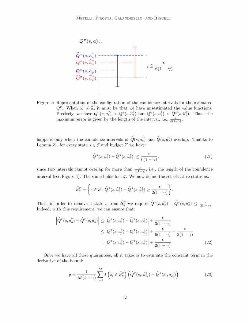
Metelli, Pirotta, Calandriello, and Restelli
Qπ(s, a)
Qπ(s, a↑s)
Qπ(s, a↑s)
Qπ(s, a↑s)
Qπ(s, a↑s)
≤ ε
6(1 − γ)
Figure 4: Representation of the configuration of the confidence intervals for the estimatedQπ. When a↑s 6= a↑s it must be that we have misestimated the value functions.Precisely, we have Qπ(s, a↑s) > Qπ(s, a↑s) but Qπ(s, a↑s) < Qπ(s, a↑s). Thus, themaximum error is given by the length of the interval, i.e., ε
6(1−γ) .
happens only when the confidence intervals of Q(s, a↑s) and Q(s, a↑s) overlap. Thanks toLemma 21, for every state s ∈ S and budget Υ we have:
∣∣∣Qπ(s, a↑s)− Qπ(s, a↑s)∣∣∣ ≤ ε
6(1− γ), (21)
since two intervals cannot overlap for more than ε6(1−γ) , i.e., the length of the confidence
interval (see Figure 4). The same holds for a↓s. We now define the set of active states as:
Sππ =
{s ∈ S : Qπ(s, a↑s)− Qπ(s, a↓s) ≥
ε
2(1− γ)
}.
Thus, in order to remove a state s from Sππ we require Qπ(s, a↑s) − Qπ(s, a↓s) ≤ ε2(1−γ) .
Indeed, with this requirement, we can ensure that:
∣∣∣Qπ(s, a↑s)− Qπ(s, a↓s)∣∣∣ ≤
∣∣∣Qπ(s, a↑s)− Qπ(s, a↓s)∣∣∣+
ε
3(1− γ)
≤∣∣∣Qπ(s, a↑s)−Qπ(s, a↓s)
∣∣∣+ε
6(1− γ)+
ε
3(1− γ)
=∣∣∣Qπ(s, a↑s)−Qπ(s, a↓s)
∣∣∣+ε
2(1− γ)(22)
Once we have all these guarantees, all it takes is to estimate the constant term in thederivative of the bound:
g =1
M(1− γ)
M∑
i=1
I(si ∈ Sππ
)(Qπ(si, a
↑si)− Qπ(si, a
↓si)). (23)
42

Safe Policy Iteration
Approach N M T Per–iteration sample complexity
aUSPI d 169ε2
log 2δ e - dlogγ
ε12e NT
aSSPI d1289ε2
log 4|S|δ e d 8
ε2log 4
δ e dlogγε8e NT |S||A|+M
aSASPI d128ε2
log 4|S||A|δ e d 288
121ε2log 4
δ e dlogγε
48e NT |S||A|+M
Table 1: Per–iteration sample complexity for the presented approximate versions of the SPIalgorithms.
Lemma 22. Let π, π ∈ ΠSR be two Markovian stationary policies for the same MDP M.Let
M =
⌈288
121ε2log
2
δ
⌉.
Under the assumptions of Lemma 19, the sampling procedure constructs a function g suchthat with probability 1− 2δ:
g − g ≤ ε
(1− γ)2.
Algorithm 11 reports the pseudocode of the FJP function for aSASPI. The samplingprocedure and Lemma 22 allow us to compute the per–iteration sample complexity. Indeed,we sample N trajectories for every state and action pair, each of length T , in order to have anestimate of Qπ(s, a) for all (s, a) ∈ S ×A. Then, we need M samples to compute g, takinga sample mean under dπ. Thus, overall we need NT |A||S| + M samples. Table 1 reportsa comparison of the per–iteration sample complexity of the approximate SPI algorithmspresented so far.
Remark 12 (Theoretical Guarantees Comparison). The theoretical guarantees that weprovide in this section aim at bounding the number of samples needed to ensure that, ateach iteration, we perform a policy update that yields a performance improvement with highprobability. These guarantees can be extended to multiple iterations, as done in Kakade(2003), to prove that the SPI algorithms stop with an expected average advantage thatsatisfies Aπ+
π ≤ κ1−γ , where κ > 0 is a threshold. This kind of requirements is quite
different compared to several employed in the literature (e.g., Azar et al., 2012, 2011; Sidfordet al., 2018; Wainwright, 2019a,b), where the goal is to provide the conditions for whichthe learned policy is κ–optimal, leading to a bound on the difference of value functions‖q∗ − q‖. The two conditions are clearly related (see for instance Lemma 7), but, webelieve, not directly comparable. Furthermore, while for aUSPI we have provided theconvergence to an optimal policy in a finite number of iterations (Theorem 17) under specificchoices of the hyperparameters, we cannot directly extend this result for aSSPI and aSASPI.Unfortunately, without further specifications on the value of ε they could stop short ofreaching the optimal policy.
6. Applications of SPI techniques
This section is devoted to the analysis of the performances of the algorithms in a discreteenvironment. The tests are mainly intended to give empirical supports to the theoretical
43

Metelli, Pirotta, Calandriello, and Restelli
Algorithm 11 Computing of the jump points for aSASPI (FJP)
input: MDP M, current policy π, target policy π, accuracy ε, confidence δ
initialize: t← 0, M ← d 288121ε2 log 4
δ e, N ← d 128ε2 log 4|S||A|
δ e, T ← dlogγε
48e, Υ0
2 ← 0, i↑, i↓ ← 0
Compute G↑(s, a) and G↓(s, a), ∀s ∈ S, ∀a ∈ ACompute the two orderings ρ↑ and ρ↓ such that s.t. i < j =⇒ G↑(sρ↑i
, aρ↑i) ≤ G↑(sρ↑j
, aρ↑j) and
i < j =⇒ G↓(sρ↓i, aρ↓i
) ≤ G↑(sρ↓j , aρ↓j )
Compute a↑s = arg maxa∈A{Qπ(s, a)
}and a↓s = arg mina∈A
{Qπ(s, a)
}, ∀s ∈ S
Sππ ← {s ∈ S : Qπ(s, a↑s)− Qπ(s, a↓s) >ε
2(1−γ)}q0 ← 1
1−γ∑s∈Sππ
12dπ(s)
(Qπ(s, a↑s)−Qπ(s, a↓s)
)− ε
1−γyield Υ0, q0
while Sππ 6= {} dot← t+ 1if st ∈ Sππ then
if G↑(sρ↑,i↑aρ↑
i↑) ≤ G↓(sρ↓
i↓, aρ↓
i↓) then
st, at ← sρ↑i↑, aρ↑
i↑
if Qπ(st, at) > Qπ(st, a↓st) + ε
2(1−γ) then
qt ← qt−1 − 12dπ(st)
(Qπ(st, a
↑sit)− Qπ(st, at)
)
a↑st ← atelse
qt ← qt−1 − 12dπ(st)
(Qπ(st, a
↑st)− Qπ(st, a
↓st))
Sππ \ {st}end ifΥt2 ← G↑(st, at)i↑ ← i↑ + 1
elsest, at ← sρ↓
i↓, aρ↓
i↓
if Qπ(st, at) < Qπ(st, a↓st)− ε
2(1−γ) then
qt ← qt−1 − 12dπ(st)
(Qπ(st, at)− Qπ(st, a
↓st))
a↓st ← atelse
qt ← qt−1 − 12dπ(st)
(Qπ(st, a
↑st)− Qπ(st, a
↓st))
Sππ \ {st}end ifΥt2 ← G↓(st, at)i↓ ← i↓ + 1
end ifend ifyield Υt, qt
end whileyield 2, −∞
results derived in the previous section, illustrating the peculiar properties of the proposedalgorithms. Moreover, the application offers some practical aspects of the implementation
44
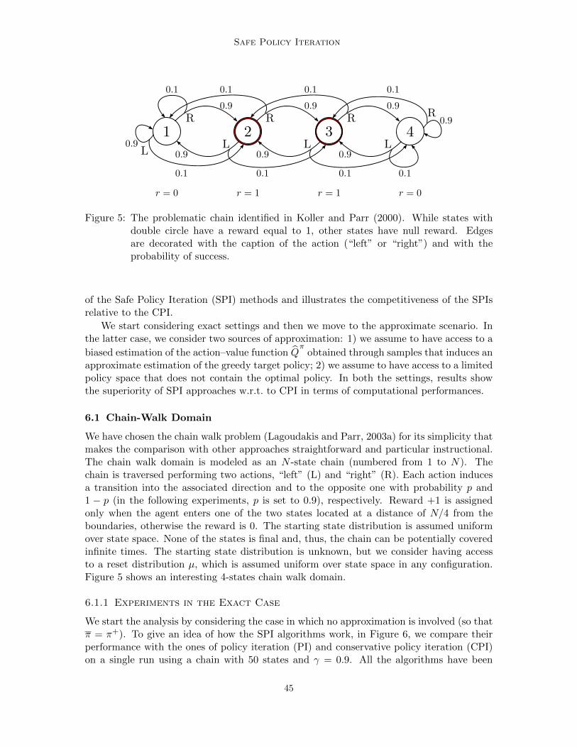
Safe Policy Iteration
Figure 5: The problematic chain identified in Koller and Parr (2000). While states withdouble circle have a reward equal to 1, other states have null reward. Edgesare decorated with the caption of the action (“left” or “right”) and with theprobability of success.
of the Safe Policy Iteration (SPI) methods and illustrates the competitiveness of the SPIsrelative to the CPI.
We start considering exact settings and then we move to the approximate scenario. Inthe latter case, we consider two sources of approximation: 1) we assume to have access to a
biased estimation of the action–value function Qπ
obtained through samples that induces anapproximate estimation of the greedy target policy; 2) we assume to have access to a limitedpolicy space that does not contain the optimal policy. In both the settings, results showthe superiority of SPI approaches w.r.t. to CPI in terms of computational performances.
6.1 Chain-Walk Domain
We have chosen the chain walk problem (Lagoudakis and Parr, 2003a) for its simplicity thatmakes the comparison with other approaches straightforward and particular instructional.The chain walk domain is modeled as an N -state chain (numbered from 1 to N). Thechain is traversed performing two actions, “left” (L) and “right” (R). Each action inducesa transition into the associated direction and to the opposite one with probability p and1 − p (in the following experiments, p is set to 0.9), respectively. Reward +1 is assignedonly when the agent enters one of the two states located at a distance of N/4 from theboundaries, otherwise the reward is 0. The starting state distribution is assumed uniformover state space. None of the states is final and, thus, the chain can be potentially coveredinfinite times. The starting state distribution is unknown, but we consider having accessto a reset distribution µ, which is assumed uniform over state space in any configuration.Figure 5 shows an interesting 4-states chain walk domain.
6.1.1 Experiments in the Exact Case
We start the analysis by considering the case in which no approximation is involved (so thatπ = π+). To give an idea of how the SPI algorithms work, in Figure 6, we compare theirperformance with the ones of policy iteration (PI) and conservative policy iteration (CPI)on a single run using a chain with 50 states and γ = 0.9. All the algorithms have been
45

Metelli, Pirotta, Calandriello, and Restelli
initialized with the policy uniform over actions. The graph shows, for each algorithm, thevalue of Jπ, the coefficient α (since SSPI and SASPI have several α coefficients, we plot theaverage of α(s) and α(s, a) respectively), the expected advantage function Aππ and the policydissimilarity ‖π − π‖1,dπ as a function of the number of iterations. As expected (since noapproximation is involved), PI converges to the optimal policy in only one iteration. At theopposite end, CPI (whose convergence to the optimal policy is asymptotic) has a very slowperformance improving rate when compared to the other algorithms. All SPI algorithmsconverge to the optimal policy in a finite number of iterations. USPI reaches the optimalpolicy in 44 iterations, while SSPI and SASPI take more than 100 iterations. It is worthnoting that, since the chain domain has only two actions, the behavior of SSPI and SASPIis exactly the same, as mentioned in Section 4.3. The faster convergence of USPI w.r.t.SSPI and SASPI, although not theoretically proved, has been empirically verified in manydifferent versions of the chain-walk domain obtained by varying the discount factor andthe number of states. We can explain this behavior by recalling that USPI exploits abetter bound w.r.t. the one of SSPI and SASPI, and, in the exact context, the advantageof choosing different convex combination coefficients for each state is not enough for SSPIand SASPI (at least in this domain) to attain the same improving rate of USPI. In orderto obtain a fair comparison with SSPI and SASPI we considered a simplified version ofUSPI, USPI-simp, that exploits the same bound used by SSPI and SASPI. We can see thatUSPI-simp converges to the optimal policy in almost 300 iterations. Figure 6 also displayshow the values of the convex combination coefficients change over the iterations for CPI,USPI, SSPI, SASPI, and USPI-simp. As expected, the value of α for CPI is always very lowand decreases with iterations. On the other hand, the coefficients for the SPI algorithmsstart to increase when the current policy approaches the greedy one. This is also justifiedby the quick drop of the expected advantage and policy dissimilarity experimented by theSPI algorithms.
We further analyze the performance of the considered algorithms for different state-space dimensions (N) and for different values of the discount factor γ. The algorithmsare tested over multiple runs, in particular 10 runs are performed starting from randompolicies. Figure 7 shows the behavior of the algorithms in terms of the distance betweenthe performance of the policy at each iteration and the optimal performance (Error). Itcan be seen that CPI is always outperformed by the SPI algorithms. At the same time,the USPI achieves a significantly higher learning behavior than SSPI,12 that leads to fasterconvergence to the optimal performance.
6.1.2 Experiments in the Approximate Case
To give a complete overview of the performance of the algorithms, we have moved to anapproximate framework. We consider the error induced by the estimation of the valuefunction via a set of samples. The dataset is built according to the technique explained inSection 5, using the theoretical values for the number of transitions to collect (i.e., N , Tand M). In the approximate scenario, the improvement rate of Approximate SSPI (aSSPI)is always faster than the one of Approximate USPI (aUSPI). Figure 8 shows a comparisonbetween aCPI, aUSPI, and aSSPI the 4-states chain walk domain, with 0.5 discount factor.
12. SASPI is not represented as its behavior is equal to that of SSPI.
46
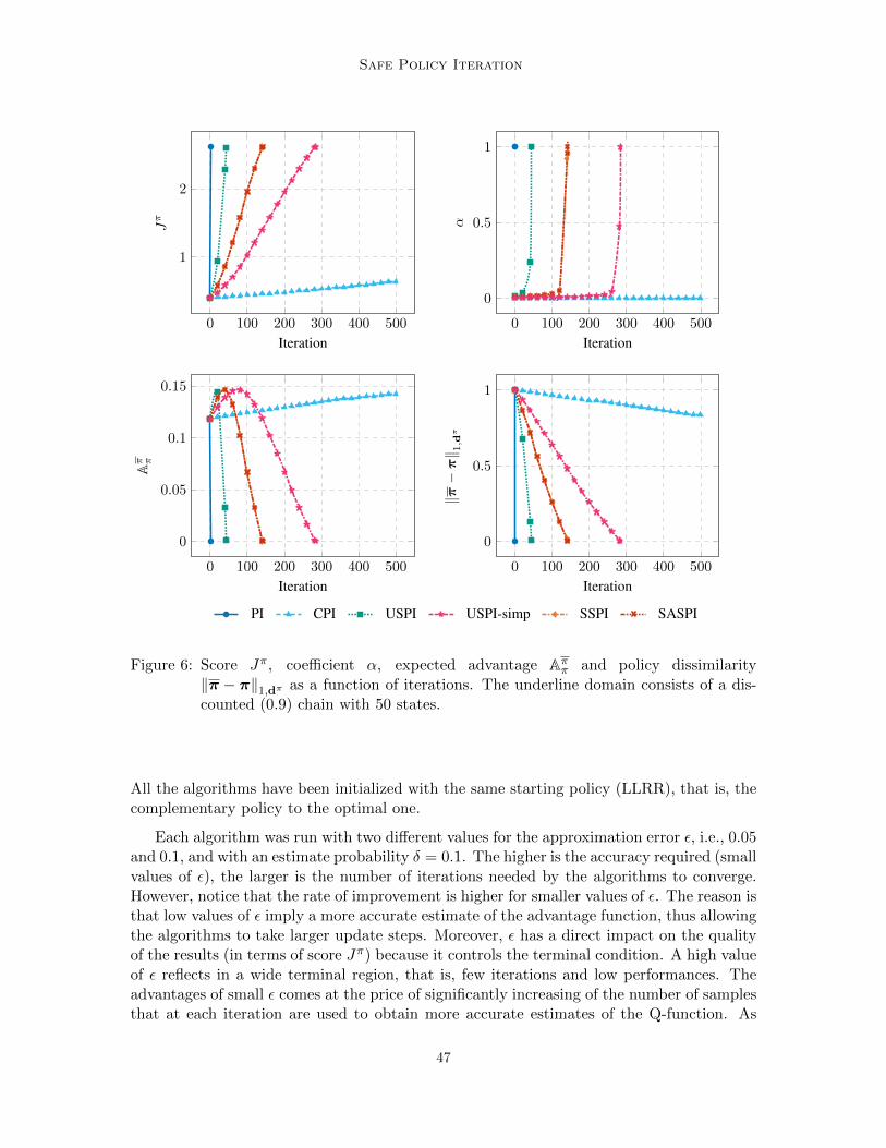
Safe Policy Iteration
0 100 200 300 400 500
1
2
Iteration
Jπ
0 100 200 300 400 500
0
0.5
1
Iteration
α
0 100 200 300 400 500
0
0.05
0.1
0.15
Iteration
Aπ π
0 100 200 300 400 500
0
0.5
1
Iteration
‖π−π‖ 1,d
π
PI CPI USPI USPI-simp SSPI SASPI
Figure 6: Score Jπ, coefficient α, expected advantage Aππ and policy dissimilarity‖π − π‖1,dπ as a function of iterations. The underline domain consists of a dis-counted (0.9) chain with 50 states.
All the algorithms have been initialized with the same starting policy (LLRR), that is, thecomplementary policy to the optimal one.
Each algorithm was run with two different values for the approximation error ε, i.e., 0.05and 0.1, and with an estimate probability δ = 0.1. The higher is the accuracy required (smallvalues of ε), the larger is the number of iterations needed by the algorithms to converge.However, notice that the rate of improvement is higher for smaller values of ε. The reason isthat low values of ε imply a more accurate estimate of the advantage function, thus allowingthe algorithms to take larger update steps. Moreover, ε has a direct impact on the qualityof the results (in terms of score Jπ) because it controls the terminal condition. A high valueof ε reflects in a wide terminal region, that is, few iterations and low performances. Theadvantages of small ε comes at the price of significantly increasing of the number of samplesthat at each iteration are used to obtain more accurate estimates of the Q-function. As
47
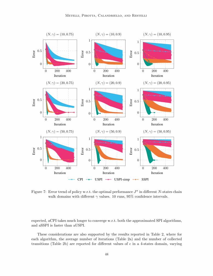
Metelli, Pirotta, Calandriello, and Restelli
0 200 400
0
0.5
Iteration
Err
or(N, γ) = (10, 0.75)
0 200 400
0
0.5
1
Iteration
Err
or
(N, γ) = (10, 0.9)
0 200 400
0
0.5
1
Iteration
Err
or
(N, γ) = (10, 0.95)
0 200 400
0
0.5
Iteration
Err
or
(N, γ) = (20, 0.75)
0 200 400
0
0.5
1
Iteration
Err
or(N, γ) = (20, 0.9)
0 200 400
0
0.5
1
Iteration
Err
or
(N, γ) = (20, 0.95)
0 200 400
0
0.5
1
Iteration
Err
or
(N, γ) = (50, 0.75)
0 200 400
0
0.5
1
Iteration
Err
or
(N, γ) = (50, 0.9)
0 200 400
0
0.5
1
Iteration
Err
or(N, γ) = (50, 0.95)
CPI USPI USPI-simp SSPI
Figure 7: Error trend of policy w.r.t. the optimal performance Jπ in different N -states chainwalk domains with different γ values. 10 runs, 95% confidence intervals.
expected, aCPI takes much longer to converge w.r.t. both the approximated SPI algorithms,and aSSPI is faster than aUSPI.
These considerations are also supported by the results reported in Table 2, where foreach algorithm, the average number of iterations (Table 2a) and the number of collectedtransitions (Table 2b) are reported for different values of ε in a 4-states domain, varying
48
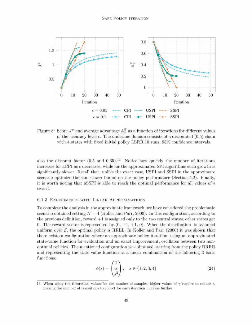
Safe Policy Iteration
0 10 20 30 40 50
0.5
1
1.5
Iteration
Jπ
0 10 20 30 40 50
0
0.2
0.4
0.6
0.8
Iteration
Aπ π
ε = 0.05 CPI USPI SSPIε = 0.1 CPI USPI SSPI
Figure 8: Score Jπ and average advantage Aππ as a function of iterations for different valuesof the accuracy level ε. The underline domain consists of a discounted (0.5) chainwith 4 states with fixed initial policy LLRR.10 runs, 95% confidence intervals.
also the discount factor (0.5 and 0.65).13 Notice how quickly the number of iterationsincreases for aCPI as ε decreases, while for the approximated SPI algorithms such growth issignificantly slower. Recall that, unlike the exact case, USPI and SSPI in the approximatescenario optimize the same lower bound on the policy performance (Section 5.2). Finally,it is worth noting that aSSPI is able to reach the optimal performance for all values of εtested.
6.1.3 Experiments with Linear Approximations
To complete the analysis in the approximate framework, we have considered the problematicscenario obtained setting N = 4 (Koller and Parr, 2000). In this configuration, according tothe previous definition, reward +1 is assigned only to the two central states, other states get0. The reward vector is represented by (0, +1, +1, 0). When the distribution is assumeduniform over S, the optimal policy is RRLL. In Koller and Parr (2000) it was shown thatthere exists a configuration where an approximate policy iteration, using an approximatedstate-value function for evaluation and an exact improvement, oscillates between two non-optimal policies. The mentioned configuration was obtained starting from the policy RRRRand representing the state-value function as a linear combination of the following 3 basisfunctions:
φ(s) =
1ss2
, s ∈ {1, 2, 3, 4} (24)
13. When using the theoretical values for the number of samples, higher values of γ require to reduce ε,making the number of transitions to collect for each iteration increase further.
49
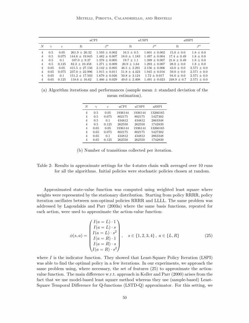
Metelli, Pirotta, Calandriello, and Restelli
aCPI aUSPI aSSPI
N γ ε It Jπ It Jπ It Jπ
4 0.5 0.05 261.9 ± 20.32 1.593 ± 0.002 16.5 ± 0.5 1.601 ± 0.002 15.0 ± 0.0 1.8 ± 0.04 0.5 0.075 144.6 ± 19.845 1.482 ± 0.007 18.0 ± 1.183 1.497 ± 0.004 17.4 ± 0.49 1.8 ± 0.04 0.5 0.1 107.0 ± 9.37 1.378 ± 0.005 19.7 ± 1.1 1.399 ± 0.007 21.6 ± 0.49 1.8 ± 0.04 0.5 0.125 82.2 ± 10.458 1.271 ± 0.009 20.9 ± 1.64 1.293 ± 0.007 28.0 ± 0.0 1.8 ± 0.04 0.65 0.05 415.5 ± 27.156 2.142 ± 0.005 46.5 ± 2.291 2.156 ± 0.006 43.0 ± 0.0 2.571 ± 0.04 0.65 0.075 237.0 ± 22.996 1.915 ± 0.011 51.8 ± 4.423 1.945 ± 0.016 59.0 ± 0.0 2.571 ± 0.04 0.65 0.1 151.2 ± 17.503 1.679 ± 0.026 50.8 ± 3.124 1.72 ± 0.017 94.0 ± 0.0 2.571 ± 0.04 0.65 0.125 118.6 ± 16.62 1.466 ± 0.029 49.0 ± 2.408 1.491 ± 0.023 248.9 ± 0.7 2.571 ± 0.0
(a) Algorithm iterations and performances (sample mean ± standard deviation of themean estimation).
N γ ε aCPI aUSPI aSSPI
4 0.5 0.05 1936144 1936144 132661654 0.5 0.075 802175 802175 54273024 0.5 0.1 434812 434812 28633484 0.5 0.125 262550 262550 17428394 0.65 0.05 1936144 1936144 132661654 0.65 0.075 802175 802175 54273024 0.65 0.1 434812 434812 28633484 0.65 0.125 262550 262550 1742839
(b) Number of transitions collected per iteration.
Table 2: Results in approximate settings for the 4-states chain walk averaged over 10 runsfor all the algorithms. Initial policies were stochastic policies chosen at random.
Approximated state-value function was computed using weighted least square whereweights were represented by the stationary distribution. Starting from policy RRRR, policyiteration oscillates between non-optimal policies RRRR and LLLL. The same problem wasaddressed by Lagoudakis and Parr (2003a) where the same basis functions, repeated foreach action, were used to approximate the action-value function:
φ(s, a) =
I(a = L) · 1I(a = L) · sI(a = L) · s2
I(a = R) · 1I(a = R) · sI(a = R) · s2
, s ∈ {1, 2, 3, 4} , a ∈ {L,R} (25)
where I is the indicator function. They showed that Least-Square Policy Iteration (LSPI)was able to find the optimal policy in a few iterations. In our experiments, we approach thesame problem using, where necessary, the set of features (25) to approximate the action-value function. The main difference w.r.t. approach in Koller and Parr (2000) arises from thefact that we use model-based least square method whereas they use (sample-based) Least-Square Temporal Difference for Q-functions (LSTD-Q) approximator. For this setting, we
50

Safe Policy Iteration
0 200 400 600
2
4
6
8
10
Iteration
Jπ
0 200 400 600
0
0.5
1
Iteration
Aπ π
aPI aCPI aUSPI aSSPI DDP aCPI-const Soft-LSPI
Figure 9: Score Jπ and average advantage Aππ as a function of iterations when consideringlinear approximators for the value function. The underline domain consists ofa discounted (0.9) chain with 4 states with fixed initial policy RRRR. A dottedline is drawn in correspondence of the value of the optimal policy. 10 runs, 95%confidence intervals.
considered additional baselines: Dynamic Policy Programming (DPP, Azar et al., 2012),CPI with constant learning rate (aCPI-const, Scherrer, 2014), and Softened-LSPI (Soft-LSPI, Perolat et al., 2016). For aCPI-const we crossvalidated the learning rate α amongthe values 0.01, 0.05, 0.1, and 0.5. Similarly, for DPP we consider the best value of theinverse temperature parameter η among 0.1, 1, and 10.
The results of the experiment can be summarized as follows. Policy iteration algorithmis confirmed to oscillate between policy LRRR and policy RLLL which both have the samesuboptimal performance. Similar behavior is displayed by Soft-LSPI, which tends to prefertoo large learning rates, importing the same problems of aPI. aCPI does not suffer from theapproximation and slowly converges (at infinity) to the optimal policy. On the other side,the proposed algorithms aUSPI and aSSPI are able to reach the optimal policy in a finitenumber of iterations without any loss of performance. aCPI-const with a learning rate setto 0.5 is able to reach the optimal performance very quickly with no oscillation phenomena.Instead, DPP, with an inverse temperature equal to 10, converges to a suboptimal policy.Furthermore, it should be noted that aCPI-const and DPP require the specification of anadditional hyperparameter (the learning rate α and the inverse temperature η), whereasthe SPI algorithms are hyperparameter free. For all algorithms, we used N = 1000 samplesand a horizon of T = 20 for estimating the value function. For aSSPI, we used 1000 sampleswith and horizon 20 for estimating the advantage function in each state and 100 samplesfor estimating the derivative of the bound to be optimized. Figure 9 presents a generaloverview of the trend of the tested algorithms.
51

Metelli, Pirotta, Calandriello, and Restelli
-0.71 -0.45 -0.32 -0.24 -0.20
-0.45 -0.19
-0.32 -1.00 -0.17
-0.24 -0.16
-0.20 -0.19 -0.17 -0.16 -0.14
0.6
Figure 10: The prison domain. The reward is depicted for wall states (dark cells) because allthe actions receive the same signal. Arrows represent the transitions associatedto the “SOUTH” action with a noise level of 0.4.
6.2 The Prison
The domain is a particular implementation of the classical grid world domain (Sutton andBarto, 2018). This variant (Azar et al., 2012) is a M–squared grid world surrounded byabsorbing states (wall states). Each state s is determined by the coordinate of the cellcs = (x, y), for some x, y = 1, . . . ,M . The wall states that surround the grid have a rewardthat grows proportionally to the distance from the bottom–right corner:
R(s, a) = − 1
‖cs‖2, ∀a ∈ A.
There is an additional absorbing state located at the center of the grid that has a rewardof −1. All the remaining inner states have a zero reward signal. Four discrete actionsA = {NORTH,SOUTH,WEST,EAST} are available in each state s. Taking an action a inan inner (non–absorbing) state s causes a transition in the direction corresponding to theaction with a probability p, and a random move in a state s′ 6= s with a probability inverselyproportional to the Euclidean distance 1
‖cs−cs′‖2. Due to the presence of absorbing states
surrounding the grid, the optimal behavior is to survive in the grid, avoiding also the centralwall. This domain is interesting due to the presence of absorbing states with negative rewardand to the presence of noise that causes many transitions from inner states. Furthermore,having more than two actions lends itself to appreciate the advantages of SASPI over SSPI.
6.2.1 Experiments in the Exact Case
We first consider a set of experiments on the prison domain with M = 5 and γ = 0.9, inthe exact case. In Figure 11 we can see a behavior that preserves the ordering, in learningspeed, of the considered algorithms, compared to the chain domain. Indeed, PI converges tothe optimal policy in a small number of iterations and among the SPI and CPI algorithms,USPI performs best. Again, we have the confirmation that the tighter bound exploited byUSPI is enough to overcome the limitation of the unique coefficient α. Similarly, CPI is the
52

Safe Policy Iteration
0 50 100 150 200 250
9
9.2
9.4
9.6
Iteration
Jπ
0 50 100 150 200 250
0
0.5
1
Iteration
α
0 50 100 150 200 250
0
0.2
0.4
0.6
Iteration
Aπ π
0 50 100 150 200 250
0
0.5
1
1.5
Iteration
‖π−
π‖ 1,d
π
PI CPI USPI SSPI SASPI
Figure 11: Score Jπ, coefficient α, expected advantage Aππ and policy dissimilarity‖π − π‖1,dπ as a function of iterations. The underline domain consists of adiscounted (0.9) prison environment in the exact setting.
worst performing algorithm. Between the latter two, we can now appreciate a difference inthe learning curve. Since the latter considers a more flexible update rule, it is able to reachthe optimal performance sooner.
6.2.2 Experiments in the Approximate Case
Compared to the Chain, the Prison domain poses significant challenges to the usage of theapproximate versions of the SPI algorithms with the theoretical values of the hyperparam-eters. The reason of these limitations reside in the large number of deterministic policiesto test, i.e., |A||S| = 4M
2 ' 1.13 · 1015 for M = 5. Even if we disregard the terminalstates, as the action is those states has no effect, we reduce to 48 = 65536 policies. For thisreason, we decided to run the considered algorithms without the theoretical values of thehyperparametes. More specifically, we employed 200 samples with horizon 50 for the policychooser, we used 50 with horizon 50 samples for estimating the state advantage function
53

Metelli, Pirotta, Calandriello, and Restelli
0 1,000 2,000 3,000
9
9.2
9.4
9.6
9.8
Iteration
Jπ
0 1,000 2,000 3,000
0
0.2
0.4
0.6
Iteration
Aπ π
aPI aCPI aUSPI aSSPI aSASPI DPP aCPI-const
Figure 12: Score Jπ and expected advantage Aππ as a function of iterations. The underlinedomain consists of a discounted (0.9) prison environment in the approximatesetting. 10 runs, 95% confidence intervals.
and the Q-function for aSSPI and aSASPI, respectively, and 50 samples for computing thebound derivative. Therefore, the number of collected transitions for aPI, aCPI, and aUSPIis 10000, while for aSSPI and aSASPI we need to collect 260050 transitions (refer to Table 1for the computation). Figure 12 shows the behavior of the compared algorithms. First ofall, we easily notice that aPI displays a considerable oscillation phenomenon, this is due tothe fact that it is continuously switching the policy between the optimal and some subop-timal policies. Instead, CPI and USPI converge slowly towards the optimal policy with asmall advantage of USPI in terms of learning speed, but they are both outperformed byaSSPI. We can see that aSASPI is able to outperform all the other SPI algorithms andreach the optimal behavior with remarkable stability. aCPI-const with α = 0.05, as wellas DPP with η = 1 reach very quickly a good performance, although aCPI-const displaysa little instability. However, both aCPI-const and DPP converge to a policy with slightlylower performance compared to that reached by aSASPI.
6.3 BlackJack Card Game
The BlackJack is a card game where the player seeks to beat the dealer by obtaining a totalscore greater than the dealer’s one without exceeding 21 (refer to Dutech et al. (2005) formore details). Each card counts as its numerical value (2 through 10) except for aces andfigures. The Jack, Queen, and King are worth 10, whereas the ace may value as either 1or 11. The value of the ace is hand such that it produces the highest value equal to or lessthan 21. A hand is called soft when the ace is counted as 11. The set of cards is composedby 6 decks each one is a standard 52–cards deck.
At the beginning of the game, the dealer deals two cards to each player, includinghimself. One card is faced up and the other is faced down. The player checks his two cardsand chooses to receiver a new card (hit) or to stop (stand). The player may ask for more
54

Safe Policy Iteration
cards as long as he does not bust, i.e., the sum of the card values does not overcome 21.When all the players go bust or stops, is the turn of the dealer. In the beginning, the playercan also decide to double the score, i.e., he does not ask for any card and let the dealer play.In this case, any score achieved by the player is doubled.
In Pirotta et al. (2013b) a simplified version, made of 260 states, of the blackjack gameby removing advanced actions as “doubling”, “splitting”, etc was considered. We nowextend those results by allowing the usage of the double action. The game is composed ofa player and a dealer. The state of the game is defined by three components: the sum ofthe cards of the player (2 to 20), the dealer’s faced-up card (1 to 10) and the soft handflag. The player is forced to play “stand” action on blackjack and on 21. Moreover, thesoft hand flag is irrelevant when player’s value is greater than 11. As a consequence, thecardinality of the state space is 260. The action space is composed of the three actions:hit (H), stand (S), and double (D). The rewards assigned to the player are +1 for winning(+1.5 for blackjack), -1 for loosing and 0 for every hit. All rewards are doubled when thedouble action is performed. Rewards have been scaled to fit the interval [0, 1].
To evaluate the performance of the algorithms, we have exploited the simplified Black-Jack model with discount factor equal to 0.814 and “stands on soft 17” strategy for thedealer. The evaluation measure is the estimated player edge, i.e., the average reward overmultiple runs. We have been able to define a configuration where an approximate policyiteration, using a sample-based policy evaluation step and an exact improvement, oscillatesbetween two non-optimal policies. This configuration has been obtained by limiting thepolicy space to three policies. Two of them are the same employed in Pirotta et al. (2013b):they select the best action (S) when player’s value is equal to 20 and opposite actions forthe other states (πS selects S and πH selects H). States with dealer’s value is at least 9 aretreated in an opposite way: policy πS selects H and policy πH chooses S. We introduce anew policy πD, which performs the double (D) action when the player’s value is 9 and thedealer’s value is between 3 and 6 or the player’s value is 10 and the dealer’s value is between2 and 9. In all other cases, πD behaves like πH . To summarize, the policies are definedaccording to the following rules:
πS =
H, if dealer’s value is greater or equal to 9
H, if player’s value is less than 1
S, otherwise
πH =
S, if dealer’s value is greater or equal to 9
S, if player’s value is greater than 19
H, otherwise
πD =
D, if player’s value is 9 and dealer’s value between 3 and 6
D, if player’s value is 10 and dealer’s value between 2 and 9
S, if player’s value is greater than 19
H, otherwise
14. We employed this value of the discount factor to mitigate the over-conservative behavior of the dissimi-larity penalization.
55

Metelli, Pirotta, Calandriello, and Restelli
0 1,000 2,000 3,000
0.15
0.2
0.25
0.3
Iteration
Jπ
0 1,000 2,000 3,000
−0.1
0
0.1
Iteration
Aπ π
aPI aCPI aUSPI aSSPI aSASPI
Figure 13: Estimated score Jπ and estimated expected advantage Aππ as a function of iter-ations. The underline domain consists of a discounted (0.8) blackjack environ-ment. 5 runs, 95% confidence intervals.
Policy πH has been chosen as initial policy. The goal of this experiment is to showthe advantages of aSSPI and aSASPI when having access to a very limited target policyspace. Indeed, by leveraging on the freedom granted by per–state and per–state–actioncombination coefficients, the effective set of policies representable by aSSPI and aSASPI islarger compared to that of aCPI and aUSPI.
Figure 13 reports the performance of the policies obtained by aPI, aCPI, aUSPI, aSSPI,and aSASPI algorithms using 1000 samples with horizon 100 for the policy chooser, weused 100 with horizon 100 samples for estimating the state advantage function and theQ-function for aSSPI and aSASPI respectively and 100 samples for computing the boundderivative. While aPI oscillates among the three policies, other algorithms do not get stuckand converge towards better policies. In particular, aCPI and aUSPI converge to a mixtureof the three policies. It is worth underlining that, in this highly stochastic domain, the aSSPIand aSASPI are able to exploit the flexibility given by the multiple convex coefficients andto converge faster than aUSPI and aCPI, getting to policies that are not representable byaCPI and aUSPI. In principle, we could exploit the transformation presented in Remark 6to allow aCPI and aUSPI to have access to the same set of policies as aSSPI and aSASPI.However, in this specific case, the number of target policies needed would be ' 1.43e+ 73,which is clearly prohibitive.15
7. Discussion and Conclusions
In this section, we discuss the contributions of this paper and we present some futureresearch directions to overcome the limitations of the proposed approaches.
15. Notice that |A||S| ' 1.13e+ 124.
56

Safe Policy Iteration
This paper builds upon (Pirotta et al., 2013b) and extends the work on the theoretical,algorithmic, and empirical sides. The main theoretical achievement, which was identified asa crucial point in Pirotta et al. (2013b), is the proof of the convergence of the SPI algorithmsin a finite number of iterations in the exact setting (Section 4.1), opposed to the (only)asymptotic convergence of CPI. We have shown that the finite convergence also extendsto the approximate setting, as long as the stopping threshold is chosen in an adaptiveway (Section 5.2). From the algorithmic point of view, we introduce a novel and moregeneral update rule based on per–state–action convex combination coefficients (SASPI,Section 4.3), that we presented in a unified framework together with SSPI (Section 4.2),which was already provided in Pirotta et al. (2013b). Moreover, we presented a completePAC analysis of the single iteration of the considered algorithms (Section 5) that extendsthe one of Pirotta et al. (2013b) and Kakade and Langford (2002), allowing for the analysisof the newly presented approaches. Finally, the empirical validation extends the resultsof Pirotta et al. (2013b) by presenting the behavior of the new algorithms in the previousdomains and the introduction of a new domain, the prison, in which the advantage of SASPIis clearly visible.
Although proved to be effective in terms of learning speed, aSSPI and aSASPI posesignificant challenges in their application to domains with a large number of states andactions. Indeed, they require to approximate the advantage function and the Q-function(possibly using independent samples) for each state and each state–action pair. To alleviatethis issue, it is possible to consider a slightly modified version of the algorithms, where thestate–action space is split into subregions (using state–action aggregation) and all the state–action pairs in a region share the advantage function or Q-function. By changing the size ofthese subregions, we can generate several different situations that range from the originalaSSPI and aSASPI approach (no aggregation) to the aUSPI one (where all the state andactions are associated with the same coefficient).
A research direction, already mentioned in Pirotta et al. (2013b), but not investigated inthis paper, is to exploit the proposed bounds to perform approximate policy iteration in theoff–policy case, i.e., when the samples have been initially collected (once for all) followingsome exploration strategy. In this case, we can use the bound in Theorem 3 where πb is theexploration strategy.
57

Metelli, Pirotta, Calandriello, and Restelli
Acknowledgments
...
Appendix A. Additional Proofs and Derivations
In this appendix, we report the proofs of the results we omitted in the main paper.
A.1 Proofs of Section 3
Corollary 4. For any stationary policies π and π′ and any starting state distribution µ, thedifference between the performance of π′ and the one of π can be lower bounded as follows:
Jπ′ − Jπ ≥ 1
1− γAπ′π −
γ
(1− γ)2
∥∥π′ − π∥∥2
∞‖qπ‖∞
2.
Proof The proof comes from a lower bound to the bound in Theorem 3 when πb = π.Such lower bound involves two upper bounds. First, we perform the upper bound:
∥∥π′ − π∥∥
1,dπ≤∥∥π′ − π
∥∥∞ .
Second, upper bound the quantitysp(aπ′π
)2 :
sp(aπ′π
)
2≤∥∥∥aπ′π
∥∥∥∞
=∥∥(π′ − π
)qπ∥∥∞
= maxs∈S
{∣∣∣∣∣∑
a∈A
(π′(a|s)− π(a|s)
)Qπ(s, a)
∣∣∣∣∣
}
≤ maxs∈S
{∥∥π′(·|s)− π(·|s)∥∥
1
sp(Qπ(s, ·))2
}
≤ maxs∈S
{∥∥π′(·|s)− π(·|s)∥∥
1
}maxs∈S
{sp(Qπ(s, ·))
2
}
≤∥∥π′ − π
∥∥∞‖qπ‖∞
2,
where the last inequality follows from the positiveness of Qπ and from norm properties.
The Corollary is proven by introducing this bound in place ofsp(aπ′π
)2 in Theorem 3 and
replacing πb with a generic π.
A.2 Proofs of Section 4
Lemma 2. (Kakade and Langford, 2002) For any stationary policies π and π′ and anystarting state distribution µ:
58
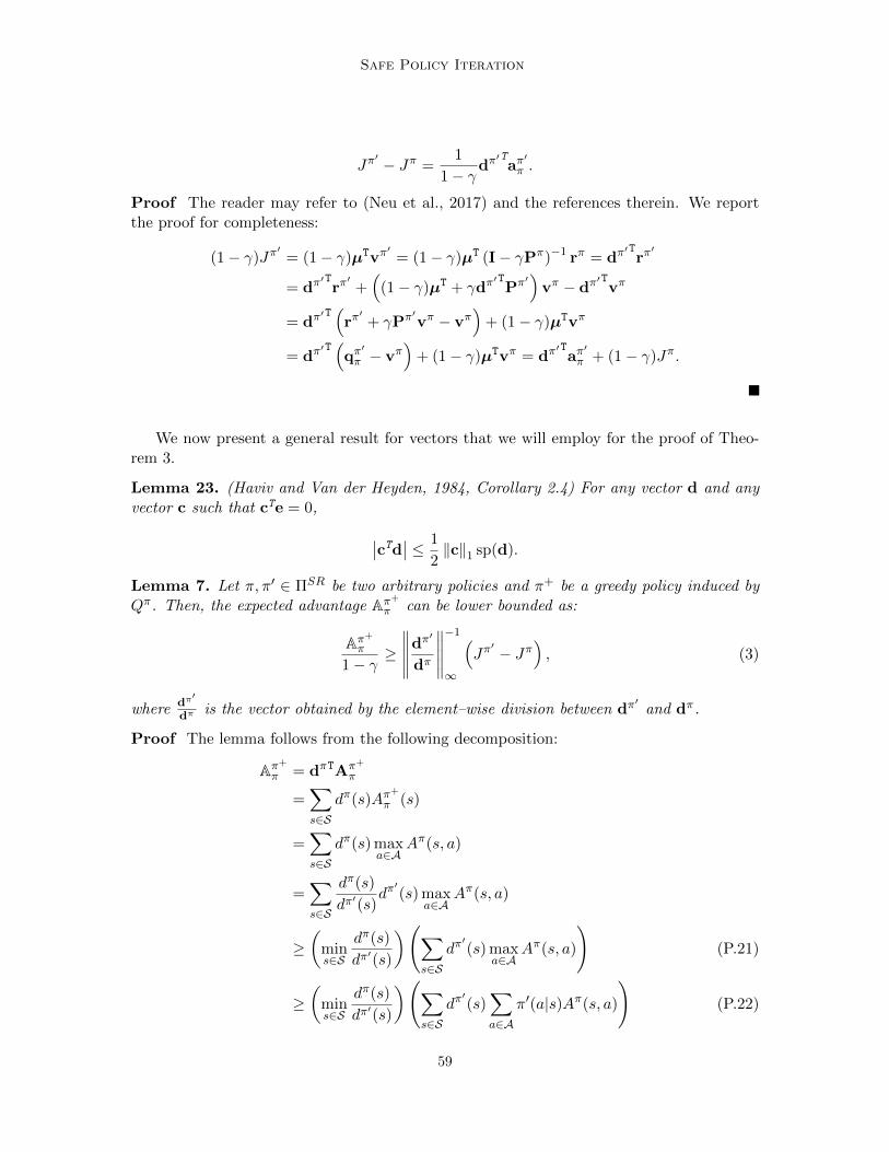
Safe Policy Iteration
Jπ′ − Jπ =
1
1− γdπ′Taπ
′π .
Proof The reader may refer to (Neu et al., 2017) and the references therein. We reportthe proof for completeness:
(1− γ)Jπ′
= (1− γ)µTvπ′
= (1− γ)µT (I− γPπ)−1 rπ = dπ′Trπ′
= dπ′Trπ′+(
(1− γ)µT + γdπ′TPπ′)vπ − dπ
′Tvπ
= dπ′T(rπ′+ γPπ′vπ − vπ
)+ (1− γ)µTvπ
= dπ′T(qπ′π − vπ
)+ (1− γ)µTvπ = dπ
′Taπ′π + (1− γ)Jπ.
We now present a general result for vectors that we will employ for the proof of Theo-rem 3.
Lemma 23. (Haviv and Van der Heyden, 1984, Corollary 2.4) For any vector d and anyvector c such that cTe = 0,
∣∣cTd∣∣ ≤ 1
2‖c‖1 sp(d).
Lemma 7. Let π, π′ ∈ ΠSR be two arbitrary policies and π+ be a greedy policy induced byQπ. Then, the expected advantage Aπ+
π can be lower bounded as:
Aπ+
π
1− γ ≥∥∥∥∥∥dπ′
dπ
∥∥∥∥∥
−1
∞
(Jπ′ − Jπ
), (3)
where dπ′
dπ is the vector obtained by the element–wise division between dπ′
and dπ.
Proof The lemma follows from the following decomposition:
Aπ+
π = dπTAπ+
π
=∑
s∈Sdπ(s)Aπ
+
π (s)
=∑
s∈Sdπ(s) max
a∈AAπ(s, a)
=∑
s∈S
dπ(s)
dπ′(s)dπ′(s) max
a∈AAπ(s, a)
≥(
mins∈S
dπ(s)
dπ′(s)
)(∑
s∈Sdπ′(s) max
a∈AAπ(s, a)
)(P.21)
≥(
mins∈S
dπ(s)
dπ′(s)
)(∑
s∈Sdπ′(s)∑
a∈Aπ′(a|s)Aπ(s, a)
)(P.22)
59

Metelli, Pirotta, Calandriello, and Restelli
=
(maxs∈S
dπ′(s)
dπ(s)
)−1∑
s∈Sdπ′(s)∑
a∈Aπ′(a|s)Aπ(s, a) (P.23)
=
∥∥∥∥∥dπ′
dπ
∥∥∥∥∥
−1
∞
dπ′TAπ′π
≥∥∥∥∥∥dπ′
dπ
∥∥∥∥∥
−1
∞
(1− γ)(Jπ′ − Jπ
), (P.24)
where (P.21) follows by observing that∑
i x(i)y(i) ≥ mini x(i)∑
i y(i), for x and y vec-tors with non negative components. (P.22) follows from the fact that maxa∈AA
π(s, a) ≥∑a∈A π
′(a|s)Aπ(s, a) for any policy π′. (P.23) derives from simply observing that mini x(i) =
(maxi{1/x(i)})−1. Finally, (P.24) is an application of Lemma 2.
Lemma 9. Assume the same setting as Theorem 8. Let ∆J = J∗ −maxπ∈ΠSD\Π∗{Jπ} bethe performance gap between the optimal policies and the second-best deterministic policy,where Π∗ = {π ∈ ΠSD : Jπ = J∗}. Then, USPI (and CPI) with GPC selects an optimalpolicy as target policy after a finite number of iterations.
Proof The result is a straightforward application of Theorem 8:
J∗ − JπN ≤ 8γ
N∆2d(1− γ)3
≤ ∆J =⇒ N ≥ 8γ
∆J∆2d(1− γ)3
.
In the following lemma, we prove that Qπ is Lipschitz continuous w.r.t. to π across allstate-action pairs. We will employ this property in the proof of Lemma 25.
Lemma 24. The Q-function Qπ(s, a) is Lipschitz continuous over the space of Markovianstationary randomized policies ΠSR in L∞-norm, for all s ∈ S and a ∈ A. For all π, π′ ∈ΠSR and for all s ∈ S and a ∈ A, it holds that:
∣∣∣Qπ′(s, a)−Qπ(s, a)∣∣∣ ≤ γ
(1− γ)2
∥∥π′ − π∥∥∞ .
Proof As for the γ-stationary distribution we look at Qπ as a function Q•(s, a) : Π → Rfor all s ∈ S and a ∈ A. Therefore, we have:
∣∣∣Qπ′(s, a)−Qπ(s, a)∣∣∣ ≤
∥∥∥qπ′ − qπ∥∥∥∞.
We now provide a bound for∥∥∥qπ′ − qπ
∥∥∥∞
. By exploiting the Bellman equation we can
write:
qπ′ − qπ = r + γPπ′qπ
′ − r− γPπqπ
60

Safe Policy Iteration
= γPπ′qπ′ − γPπ′qπ
′ ± γPπqπ
= γPπ′(qπ′ − qπ
)+ γ
(Pπ′ −Pπ
)qπ.
Now, we can take the L∞–norm and we obtain:
∥∥∥qπ′ − qπ′∥∥∥ ≤ γ
∥∥∥Pπ′∥∥∥∞
∥∥∥qπ′ − qπ∥∥∥∞
+ γ∥∥∥Pπ′ −Pπ
∥∥∥∞‖qπ‖∞
≤ γ∥∥∥qπ′ − qπ
∥∥∥∞
+γ
1− γ∥∥∥Pπ′ −Pπ
∥∥∥∞
≤ γ
(1− γ)2
∥∥∥Pπ′ −Pπ∥∥∥∞
≤ γ
(1− γ)2‖P‖∞
∥∥π′ − π∥∥∞
=γ
(1− γ)2
∥∥π′ − π∥∥∞ .
The following technical result is employed in the proof of Lemma 10, i.e., to prove thatthe expected advantage can be lower–bounded by a function of the distance between thecurrent policy π and the greedy policy π+.
Lemma 25. Assume the same setting as Lemma 9. Let π∗ be an optimal policy and π0 ∈ Πa suboptimal policy such that J∗ −∆J ≤ Jπ0 ≤ J∗. Let η ∈ [0, 1] and π = ηπ∗ + (1− η)π0.Then, there exists a state s ∈ S and a constant ∆+ > 0 independent of η, such that thefunction:
gs(π) =∑
a∈A\{a+s }
π0(a|s)(Qπ(s, a+
s )−Qπ(s, a))≥ ∆+, (26)
where a+s ∈ arg maxa∈A {Qπ(s, a)} is a greedy action w.r.t. Qπ(s, a).
Proof The proof is divided in two parts. We first prove that for any s ∈ S, gs is continuousover the set of policies Π = {ηπ∗+ (1− η)π0 : η ∈ [0, 1]} and then we show that there existsa state s− in which gs− it is strictly positive for any η ∈ [0, 1]. Being Π a compact set, fromWeierstrass theorem, it follows that gs− admits a positive minimum.
Continuity of gs. Since the dependence on η is only in the term Qπ(s, a+s ) − Qπ(s, a),
all it takes is to prove that it is a continuous function over Π. By recalling that the greedyaction a+
s is the one that maximizes Qπ(s, ·) we have:
Qπ(s, a+s )−Qπ(s, a) = max
a∈A{Qπ(s, a)} −Qπ(s, a).
Since Qπ(s, a) is continuous for Lemma 24 and the maximum of a continuous function iscontinuous we have that Qπ(s, a+
s )−Qπ(s, a) is continuous. gs(π) is obtained by applyingtransformations that preserve continuity.
Positivity gs. By definition gs(π) ≥ 0. Suppose by contradiction that gs(π) = 0 forall s ∈ S. Thus, in all states s ∈ S and for all actions a ∈ A \ {a+
s } we have that eitherπ0(a|s) = 0 or Qπ(s, a+
s ) = Qπ(s, a). If in all states s ∈ S and for all actions a ∈ A \ {a+s }
61

Metelli, Pirotta, Calandriello, and Restelli
we have that π0(a|s) = 0, then π0 gives probability one to greedy actions, i.e., π0 = π+.Note that π+ is optimal, since we are in the setting of Lemma 9, and thus π0 is optimal,which is a contradiction. Thus, there must exist a state at least one state s− and at leastone action a−s such that π0(a−s |s−) > 0. Now, suppose that for all those states s− and forall those actions a−s , we had Qπ(s, a+
s ) = Qπ(s−, a−s ). It means that a−s is greedy and thusoptimal. Therefore, π0 is optimal, which is a contradiction.
Lemma 10. Assume the same setting as Lemma 9. It π∗ is a deterministic optimal policy,then, there exists a constant ∆+ > 0 such that:
Aπ∗π ≥
∆d∆+
2‖π∗ − π‖∞ . (4)
Proof The Lemma follows from the following decomposition:
Aπ∗π = dπTAπ∗
π
= dπT (π∗ − π)qπ
= (1− η)dπT (π∗ − π0)qπ (P.25)
= (1− η)∑
s∈Sdπ(s)
∑
a∈A(π∗(a|s)− π0(a|s))Qπ(s, a)
= (1− η)∑
s∈Sdπ(s)
(1− π0(a∗s|s))Qπ(s, a∗s)−
∑
a∈A\{a∗s}
π0(a|s)Qπ(s, a)
(P.26)
= (1− η)∑
s∈Sdπ(s)
∑
a∈A\{a∗s}
π0(a|s) (Qπ(s, a∗s)−Qπ(s, a)) (P.27)
≥ (1− η) mins∈S{dπ(s)}
∑
s∈S
∑
a∈A\{a∗s}
π0(a|s) (Qπ(s, a∗s)−Qπ(s, a)) (P.28)
≥ (1− η) mins∈S{dπ(s)}max
s∈S
∑
a∈A\{a∗s}
π0(a|s) (Qπ(s, a∗s)−Qπ(s, a))
(P.29)
≥ (1− η) mins∈S{dπ(s)}max
s∈S{gs(π)} (P.30)
≥ (1− η)∆d∆+ (P.31)
= ∆d∆+‖π∗ − π‖∞‖π∗ − π0‖∞
(P.32)
≥ ∆d∆+
2‖π∗ − π‖∞ , (P.33)
We now explain the steps of the derivation. (P.25) follows from observing that π =ηπ∗ + (1 − η)π0 and so π∗ − π = (1 − η) (π∗ − π0). (P.26) is obtained by observing thatthe optimal policy is unique and deterministic; whereas (P.27) derives from observing that1− π0(a∗s|s) =
∑a∈A\{a∗s} π0(a|s). (P.28) is obtained from
∑i x(i)y(i) ≥ mini x(i)
∑i y(i),
for x and y vectors with non negative components; while (P.29) exploits the trivial re-lation
∑i y(i) ≥ maxi y(i). (P.30) simply exploits the definition of gs(π) as defined in
62

Safe Policy Iteration
Lemma 25 and (P.31) applies Lemma 25. (P.32) derives from the fact that ‖π∗ − π‖∞ =(1− η)‖π∗ − π0‖∞ and (P.33) by bounding ‖π∗ − π0‖∞ ≤ 2.
A.3 Proofs of Section 5
The following result upper–bounds the error, in L1-norm, when approximating the infinite-horizon γ-discounted stationary distribution with a finite horizon T .
Lemma 26. Let dπ be the infinite-horizon γ-discounted stationary distribution and dπT bethe T -horizon γ-discounted stationary distribution, then it holds that:
‖dπ − dπT ‖1 ≤ 2γT .
Proof We use the definition of dπ and dπT :
‖dπ − dπT ‖1 =∑
s∈S
∣∣∣∣(1− γ)
+∞∑
t=0
γt Pr (st = s|π,M)− 1− γ1− γT
H−1∑
t=0
γt Pr (st = s|π,M)
∣∣∣∣
≤ (1− γ)∑
s∈S
∣∣∣∣∣+∞∑
t=T
γt Pr (st = s|π,M)
∣∣∣∣∣+1− γ
1− γT γT∑
s∈S
∣∣∣∣∣T−1∑
t=0
γt Pr (st = s|π,M)
∣∣∣∣∣
≤ (1− γ)
+∞∑
t=T
γt∑
s∈SPr (st = s|π,M) +
1− γ1− γT γ
TT−1∑
t=0
γt∑
s∈SPr (st = s|π,M)
= (1− γ)+∞∑
t=T
γt +1− γ
1− γT γTT−1∑
t=0
γt
= (1− γ)γT
1− γ +1− γ
1− γT γT 1− γT
1− γ = 2γT ,
where we exploited the fact that∑
s∈S Pr (st = s|π,M) = 1 for every t and we used theproperties of the geometric series.
We now bound the error introduced when considering finite trajectories of horizon T inthe estimation of the action-value function.
Lemma 27. Let qπ be the infinite-horizon action-value function and qπT be the T -horizonaction-value function, then it holds that:
‖qπ − qπT ‖∞ ≤γT
1− γ .
Proof We exploit the definition of the involved quantities. For any state s and action a itholds that:
Qπ(s, a)−QπT (s, a) = Est+1∼P(·|st,at)at+1∼π(·|st+1)
[ ∞∑
t=0
γtR(st, at)|s0 = s, a0 = a
]
63

Metelli, Pirotta, Calandriello, and Restelli
− Est+1∼P(·|st,at)at+1∼π(·|st+1)
[T−1∑
t=0
γtR(st, at)|s0 = s, a0 = a
]
= Est+1∼P(·|st,at)at+1∼π(·|st+1)
[ ∞∑
t=T
γtR(st, at)|s0 = s, a0 = a
]
≤ ‖r‖∞∞∑
t=T
γt ≤ γT
1− γ ,
where we exploited the fact that ‖r‖∞ ≤ 1.
Lemma 18. Let π, π ∈ ΠSR be two Markovian stationary policies for the same MDP M.Let
T =
⌈logγ
ε
12
⌉and N =
⌈16
9ε2log
2
δ
⌉.
The aUSPI Sampling Procedure construct a function Aππ such that with probability 1− δ:∣∣∣Aππ − Aππ
∣∣∣ ≤ ε
1− γ .
Proof The proof is analogous to that of Lemma 15. First, we define the expected advantagefunction computed with horizon T :
Aππ,T = Qππ,T −Qπ
π,T .
Also in this case our estimation Aππ is unbiased for Aππ,T . We now partition the errorhighlighting the bias terms:
∣∣∣Aππ − Aππ∣∣∣ ≤
∣∣∣Aππ − Aππ,T∣∣∣
(E1)
+∣∣Aππ,T − Aππ
∣∣(E2)
.
We now require that E1 = 3ε4(1−γ) and E2 = ε
4(1−γ) , so that E1 = E2 = ε1−γ . Then,
we apply Hoeffding’s inequality to bound the deviation E1, by observing that the terms
(π(a|s)− π(a|s)) qi in the estimation Aππ are all independent and belong to[− 1
1−γ ,1
1−γ
].
Therefore, we have:
Pr
(∣∣∣Aππ − Aππ,T∣∣∣ ≥ 3ε
4(1− γ)
)≤ 2e
−2
(3ε
4(1−γ)
)2N2∑N
i=1(bi−ai)2
= 2e− 18ε2N2(1−γ)2
32(1−γ)2N = 2e−9ε2N16 .
From which we get:
e−9ε2N16 ≤ δ
2=⇒ 9ε2N
16≤ − log
δ
2=⇒ N ≥ 16
9ε2log
2
δ.
64

Safe Policy Iteration
For E2 we observe that:
∣∣Aππ,T − Aππ∣∣ =
∣∣∣∣ Es∼dπT
[Aππ,T (s)
]− Es∼dπ
[Aππ(s)
]± Es∼dπ
[Aππ,T (s)
]∣∣∣∣
≤∣∣∣∣ Es∼dπT
[Aππ,T (s)
]− Es∼dπ
[Aππ,T (s)
]∣∣∣∣+
∣∣∣∣ Es∼dπ
[Aππ(s)−Aππ,T (s)
]∣∣∣∣
≤ 1
1− γ ‖dπ − dπT ‖1 +
∣∣∣∣∣ Es∼dπ
[∑
a∈A(π(a|s)− π(a|s)) (Qπ(s, a)−QπT (s, a))
]∣∣∣∣∣
≤ 2γT
1− γ +1
2E
s∼dπ[‖π(·|s)− π(·|s)‖1 sp(Qπ(s, ·)−QπT (s, ·))]
≤ 2γT
1− γ +γT
1− γ =3γT
1− γ ,
where we exploited Lemma 23 in the last but one line and Lemma 27 in the last line. Thus,by selecting T = dlogγ
ε12e we have that the bias E2 is bounded by ε
4(1−γ) .
Lemma 19. Let π, π ∈ ΠSR be two Markovian stationary policies for the same MDP M.Let
T =
⌈logγ
ε
8
⌉and N =
⌈128
9ε2log
2|S|δ
⌉.
The aSSPI Sampling Procedure constructs a function Aππ(s) such that with probability 1− δ,simultaneously for all s ∈ S:
∣∣∣Aππ(s)−Aππ(s)∣∣∣ ≤ ε
2(1− γ).
Proof Similarly to the proof of Lemma 15, we define the expected advantage functioncomputed with horizon T :
Aππ,T (s) =∑
a∈A(π(a|s)− π(a|s))QπT (s, a),
where QπT is the action-value function cut at horizon T . Once again, our estimator Aππ isunbiased for Aππ,T . Therefore, we partition the error into:
∣∣∣Aππ(s)−Aππ(s)∣∣∣ ≤
∣∣∣Aππ(s)−Aππ,T (s)∣∣∣
(E1)
+∣∣Aππ,T (s)−Aππ(s)
∣∣(E2)
.
We set E1 = 3ε8(1−γ) and E2 = ε
8(1−γ) so that E1 +E2 = ε2(1−γ) . Then, we apply Hoeffding’s
inequality to bound the deviation E1, by observing that∑
a∈A (π(a|s)− π(a|s)) qi(s, a)
involved in the estimation Aππ(s) are all independent and belong to[− 1
1−γ ,1
1−γ
]. Therefore,
we have:
Pr
(∣∣∣Aππ(s)−Aππ,T (s)∣∣∣ ≥ 3ε
8(1− γ)
)≤ 2e
−2
(3ε
8(1−γ)
)2N2∑N
i=1(bi−ai)2
= 2e− 18ε2N2(1−γ)2
256(1−γ)2N = 2e−9ε2N128 .
65

Metelli, Pirotta, Calandriello, and Restelli
Taking the union bound over the state space S we have to solve for N
2|S|e− 9ε2N128 ≤ δ =⇒ N ≥ 128
9ε2log
2|S|δ.
We now manage the bias E2 due to the finite horizon:
∣∣Aππ,T (s)−Aππ(s)∣∣ =
∣∣∣∣∣∑
a∈A(π(a|s)− π(a|s)) (QπT (s, a)−Qπ(s, a))
∣∣∣∣∣
≤ 1
2‖π(·|s)− π(·|s)‖1 sp(QπT (s, ·)−Qπ(s, ·))
≤ ‖qπ − qπT ‖∞ ≤γT
1− γ ,
where we exploited Lemma 23 in the second line and Lemma 27 in the last line. Thus, byselecting T = dlogγ
ε8e we have that the bias E2 is bounded by ε
8(1−γ) .
The following is an intermediate result that is employed for the proof of Lemma 20.
Lemma 28. Let π, π ∈ Π be two Markovian stationary policies for the same MDP M. Let
T =
⌈logγ
ε
8
⌉and N =
⌈128
9ε2log
2|S|δ
⌉.
The sampling procedure constructs a function Aππ(s) such that with probability 1− δ, simul-taneously for all s ∈ S: ∣∣∣Aππ(s)−Aππ(s)
∣∣∣‖π(·|s)− π(·|s)‖1
≤ ε
2(1− γ).
Proof The proof is not dissimilar from that of Lemma 18. We partition the error into:∣∣∣Aππ(s)−Aππ(s)
∣∣∣‖π(·|s)− π(·|s)‖1
≤
∣∣∣Aππ(s)−Aππ,T (s)∣∣∣
‖π(·|s)− π(·|s)‖1(E1)
+
∣∣∣Aππ,T (s)−Aππ(s)∣∣∣
‖π(·|s)− π(·|s)‖1(E2)
.
We set E1 = 3ε8(1−γ) and E2 = ε
8(1−γ) so that E1 +E2 = ε2(1−γ) . Then, we apply Hoeffding’s
inequality to bound the deviation E1. We first bound uniformly the terms involved in thesample mean: ∣∣∑
a∈A (π(a|s)− π(a|s)) qi(s, a)∣∣
‖π(·|s)− π(·|s)‖1≤ 1
1− γ . (P.34)
Therefore, we can apply Hoeffding’s inequality with ranges[− 1
1−γ ,1
1−γ
]:
Pr
∣∣∣Aππ(s)−Aππ,T (s)∣∣∣
‖π(·|s)− π(·|s)‖1≥ 3ε
8(1− γ)
≤ 2e
−2
(3ε
8(1−γ)
)2N2∑N
i=1(bi−ai)2
= 2e− 18ε2N2(1−γ)2
256(1−γ)2N = 2e−9ε2N128 .
66
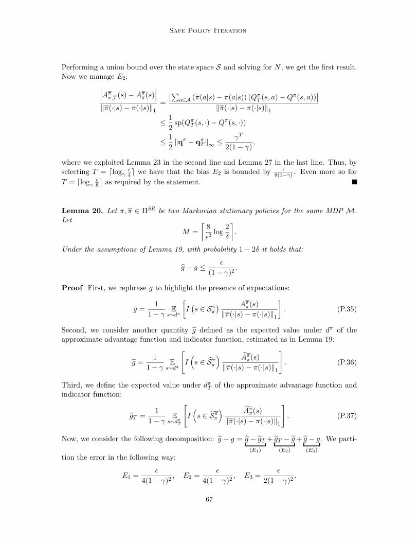
Safe Policy Iteration
Performing a union bound over the state space S and solving for N , we get the first result.Now we manage E2:
∣∣∣Aππ,T (s)−Aππ(s)∣∣∣
‖π(·|s)− π(·|s)‖1=
∣∣∑a∈A (π(a|s)− π(a|s)) (QπT (s, a)−Qπ(s, a))
∣∣‖π(·|s)− π(·|s)‖1
≤ 1
2sp(QπT (s, ·)−Qπ(s, ·))
≤ 1
2‖qπ − qπT ‖∞ ≤
γT
2(1− γ),
where we exploited Lemma 23 in the second line and Lemma 27 in the last line. Thus, byselecting T = dlogγ
ε4e we have that the bias E2 is bounded by ε
8(1−γ) . Even more so for
T = dlogγε8e as required by the statement.
Lemma 20. Let π, π ∈ ΠSR be two Markovian stationary policies for the same MDP M.Let
M =
⌈8
ε2log
2
δ
⌉.
Under the assumptions of Lemma 19, with probability 1− 2δ it holds that:
g − g ≤ ε
(1− γ)2.
Proof First, we rephrase g to highlight the presence of expectations:
g =1
1− γ Es∼dπ
[I(s ∈ Sππ
) Aππ(s)
‖π(·|s)− π(·|s)‖1
]. (P.35)
Second, we consider another quantity g defined as the expected value under dπ of theapproximate advantage function and indicator function, estimated as in Lemma 19:
g =1
1− γ Es∼dπ
[I(s ∈ Sππ
) Aππ(s)
‖π(·|s)− π(·|s)‖1
]. (P.36)
Third, we define the expected value under dπT of the approximate advantage function andindicator function:
gT =1
1− γ Es∼dπT
[I(s ∈ Sππ
) Aππ(s)
‖π(·|s)− π(·|s)‖1
]. (P.37)
Now, we consider the following decomposition: g − g = g − gT(E1)
+ gT − g(E2)
+ g − g(E3)
. We parti-
tion the error in the following way:
E1 =ε
4(1− γ)2, E2 =
ε
4(1− γ)2, E3 =
ε
2(1− γ)2.
67

Metelli, Pirotta, Calandriello, and Restelli
Let us start with E1, by observing that g is an unbiased estimator for gT :
g − gT =1
M(1− γ)
M∑
i=1
I(si ∈ Sππ
) Aππ(si)
‖π(·|si)− π(·|si)‖1
− 1
1− γ Es∼dπT
[I(s ∈ Sππ
) Aππ(s)
‖π(·|s)− π(·|s)‖1
].
If we rename f(s) = 11−γ I
(s ∈ Sππ
)Aππ(s)
‖π(·|s)−π(·|s)‖1, we are comparing a sample mean g and
the corresponding expectation g. Notice that, although f(s) are random variables as wellthey are independent of the samples si ∼ dπT . First, we provide a uniform bound of f(si)
and then we apply Hoeffding’s inequality. When s /∈ Sππ , we have f(si) = 0. Otherwise,by definition of Sππ , we have Aππ(si) ≥ ε
2(1−γ) and, in particular, f(si) ≥ 0. We now upper
bound f(si):
f(si) ≤1
1− γAππ(si)
‖π(·|si)− π(·|si)‖1
=1
1− γ
∣∣∑a∈A (π(a|si)− π(a|si)) qi(s, a)
∣∣∑
a∈A |π(a|si)− π(a|si)|
≤ 1
(1− γ)2
∑a∈A |π(a|si)− π(a|si)|∑a∈A |π(a|si)− π(a|si)|
=1
(1− γ)2.
Thus for all si we have that f(si) ranges in[0, 1
(1−γ)2
]. Therefore, we can apply Hoeffding’s
bound:
Pr
(|g − gT | ≥
ε
4(1− γ)2
)≤ 2 exp
−
2(
ε4(1−γ)2
)2M
1(1−γ)4
≤ 2 exp
(−ε
2M
8
),
from which we get the value of M . Let us now consider E2:
gT − g =1
1− γ Es∼dπT
[I(s ∈ Sππ
) Aππ(s)
‖π(·|s)− π(·|s)‖1
]
− 1
1− γ Es∼dπ
[I(s ∈ Sππ
) Aππ(s)
‖π(·|s)− π(·|s)‖1
].
We can bound the absolute value of the difference by recalling that |f(si)| ≤ 1(1−γ)2
andusing Lemma 26:
|gT − g| ≤1
(1− γ)2‖dπ − dπT ‖1 ≤
2γT
(1− γ)2.
Then, by selecting T = dlogγε8e, we are guaranteed that |gT − g| ≤ ε
4(1−γ)2Let us now
consider E3. First observe that with probability at least 1 − δ, Sππ is a subset of Sππ and
68

Safe Policy Iteration
thus I(s ∈ Sππ
)≤ I
(s ∈ Sππ
). Therefore, we have:
g − g =1
1− γ Es∼dπ
[I(s ∈ Sππ
) Aππ(s)
‖π(·|s)− π(·|s)‖1
]− Es∼dπ
[I(s ∈ Sππ
) Aππ(s)
‖π(·|s)− π(·|s)‖1
]
≤ 1
1− γ Es∼dπ
[I(s ∈ Sππ
) Aππ(s)
‖π(·|s)− π(·|s)‖1
]− Es∼dπ
[I(s ∈ Sππ
) Aππ(s)
‖π(·|s)− π(·|s)‖1
]
=1
1− γ Es∼dπ
I(s ∈ Sππ
)
‖π(·|s)− π(·|s)‖1
(Aππ(s)−Aππ(s)
)
≤ 1
1− γ Es∼dπ
∣∣∣Aππ(s)−Aππ(s)∣∣∣
‖π(·|s)− π(·|s)‖1
.
This term can be treated in way similar to what done in Lemma 19. Lemma 28 proofsthat, with probability at least 1 − δ and estimating Aππ(s) with N samples and horizon Tas defined in Lemma 19 we have that, simultaneously for all states s ∈ S:
∣∣∣Aππ(s)−Aππ(s)∣∣∣
‖π(·|s)− π(·|s)‖1≤ 5ε
12(1− γ)=⇒ g − g ≤ ε
2(1− γ)2.
Observing that we combined two results that hold with probability at least 1− δ, the state-ment holds with probability at least 1− 2δ.
Lemma 21. Let π, π ∈ ΠSR be two Markovian stationary policies for the same MDP M.Let
T =
⌈logγ
ε
48
⌉and N =
⌈128
ε2log
2|S||A|δ
⌉.
The sampling procedure constructs a function Qπ(s, a) such that with probability 1 − δ,simultaneously for all s ∈ S:
∣∣∣Qπ(s, a)−Qπ(s, a)∣∣∣ ≤ ε
12(1− γ)
Proof Similarly to the proof of Lemma 15, we partition the error into E1 = ε16(1−γ) and
E2 = ε48(1−γ) , so that E1 = E2 = ε
12(1−γ) . Then, we apply Hoeffding’s inequality to bound
the deviation, by observing that the terms qi(s, a) involved in the estimation Aππ(s) are all
independent and belong to[0, 1
1−γ
]. Therefore, we have:
Pr
(∣∣∣Qπ(s, a)−QπT (s, a)∣∣∣ ≥ ε
16(1− γ)
)≤ 2e
−2
(ε
(1−γ)
)2N2∑N
i=1(bi−ai)2
= 2e− 2ε2N2(1−γ)2
256(1−γ)2N = 2e−ε2N128 .
69

Metelli, Pirotta, Calandriello, and Restelli
Taking the union bound over the state–action space S ×A and solving for N , we get:
2|S||A|e− ε2N128 ≤ δ =⇒ N ≥ 128
ε2log
2|S||A|δ
.
We now manage the bias introduced by the truncation on length T :
|QπT (s, a)−Qπ(s, a)| ≤ γT
1− γ .
By selecting T = dlogγε
48e we have that the bias E2 is bounded by ε48(1−γ) .
Lemma 22. Let π, π ∈ ΠSR be two Markovian stationary policies for the same MDP M.Let
M =
⌈288
121ε2log
2
δ
⌉.
Under the assumptions of Lemma 19, the sampling procedure constructs a function g suchthat with probability 1− 2δ:
g − g ≤ ε
(1− γ)2.
Proof The proof is analogous to that of Lemma 20. Let us first rephrase g:
g =1
1− γ Es∼dπ
[I(s ∈ Sππ
) (Qπ(s, a↑s)−Qπ(s, a↓s
)].
We now define g and gT in a way analogous to Lemma 20:
g =1
1− γ Es∼dπ
[I(s ∈ Sππ
)(Qπ(s, a↑s)− Qπ(s, a↓s
)],
g =1
1− γ Es∼dπT
[I(s ∈ Sππ
)(Qπ(s, a↑s)− Qπ(s, a↓s
)].
Again we decompose the error into: g − g = g − gT(E1)
+ gT − g(E2)
+ g − g(E3)
and we partition the
error in the following way:
E1 =11ε
24(1− γ)2, E2 =
ε
24(1− γ)2, E3 =
1ε
2(1− γ)2.
Concerning E1, having observed that I(s ∈ Sππ
)(Qπ(s, a↑s)− Qπ(s, a↓s
)∈[0, 1
1−γ
], we can
apply Hoeffding’s inequality, as in Lemma 20:
Pr
(|g − gT | ≥
11ε
24(1− γ)2
)≤ 2 exp
−
2(
11ε24(1−γ)2
)2M
1(1−γ)4
≤ 2 exp
(−242ε2M
576
)
70
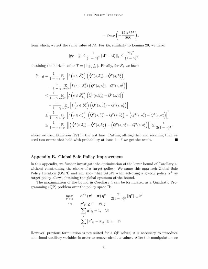
Safe Policy Iteration
= 2 exp
(−121ε2M
288
),
from which, we get the same value of M . For E2, similarly to Lemma 20, we have:
|gT − g| ≤1
(1− γ)2‖dπ − dπT ‖1 ≤
2γT
(1− γ)2,
obtaining the horizon value T = dlogγε
48e. Finally, for E3 we have:
g − g =1
1− γ Es∼dπ
[I(s ∈ Sππ
)(Qπ(s, a↑s)− Qπ(s, a↓s
)]
− 1
1− γ Es∼dπ
[I(s ∈ Sππ
) (Qπ(s, a↑s)−Qπ(s, a↓s
)]
≤ 1
1− γ Es∼dπ
[I(s ∈ Sππ
)(Qπ(s, a↑s)− Qπ(s, a↓s
)]
− 1
1− γ Es∼dπ
[I(s ∈ Sππ
)(Qπ(s, a↑s)−Qπ(s, a↓s
)]
≤ 1
1− γ Es∼dπ
[I(s ∈ Sππ
) ∣∣∣(Qπ(s, a↑s)− Qπ(s, a↓s
)−(Qπ(s, a↑s)−Qπ(s, a↓s
)∣∣∣]
≤ 1
1− γ Es∼dπ
[∣∣∣(Qπ(s, a↑s)− Qπ(s, a↓s
)−(Qπ(s, a↑s)−Qπ(s, a↓s
)∣∣∣]≤ ε
2(1− γ)2,
where we used Equation (22) in the last line. Putting all together and recalling that weused two events that hold with probability at least 1− δ we get the result.
Appendix B. Global Safe Policy Improvement
In this appendix, we further investigate the optimization of the lower bound of Corollary 4,without constraining the choice of a target policy. We name this approach Global SafePolicy Iteration (GSPI) and will show that SASPI when selecting a greedy policy π+ astarget policy allows obtaining the global optimum of the bound.
The maximization of the bound in Corollary 4 can be formulated as a Quadratic Pro-gramming (QP) problem over the policy space Π:
maxπ′∈Π
dπT(π′ − π
)qπ − γ
2(1− γ)2‖qπ‖∞ z2
s.t. π′ij ≥ 0, ∀i, j∑
j
π′ij = 1, ∀i∑
j
∣∣π′ij − πij∣∣ ≤ z, ∀i
However, previous formulation is not suited for a QP solver, it is necessary to introduceadditional auxiliary variables in order to remove absolute values. After this manipulation we
71

Metelli, Pirotta, Calandriello, and Restelli
obtain a QP problem with 2|S||A| variables. While QP problems can be solved using interiorpoint approaches (Boyd and Vandenberghe, 2004), we are going to present an iterativealgorithm that is able to attain the optimal solution and presents lower computationalcomplexity.
We adopt an approach analogous to that of SSPI and SASPI. If we were able to computethe optimal budget Υ ∗, then we can move probability across actions provided that we satisfy‖π′ − π‖∞ ≤ Υ ∗. The natural choice consists in trying to move as much probability aspossible on the action with highest Qπ, i.e., to one of the greedy actions a+
s , while takingaway probability from the suboptimal actions, starting from the worst action and followingan increasing order. The amount of probability we can move around is bounded by Y/2,that we assume fixed. Let us start by stating the following optimality condition.
Corollary 29. Let Sππ be the subset of states dπ(s) is positive: Sππ = {s ∈ S : dπ(s) > 0}.Let A+
s = {a ∈ A : Qπ(s, a) = maxa′∈AQπ(s, a′)} be the set of greedy actions in state s ∈ S
and let a+s ∈ A+
s . The bound in Corollary 4 is optimized any of the policies π′ defined as:
π′(a|s) =
{min
{Υ ∗2 , 1− π (a|s)
}if a = a+
s
max{
0,min{π(a|s), Υ2 −G↓ (s, a)
}}otherwise
,
where Υ ∗ is the value that maximizes the following function:
B(Υ ) =1
1− γ∑
s∈Sππ
dπ(s) min
{Υ
2, 1− π
(a+s | s)}
Qπ(s, a+s )
− 1
1− γ∑
s∈Sππ
dπ(s)∑
a∈A\{a+s }max
{0,min
{π (a| s) , Υ
2−G↑(s, a)
}}Qπ(s, a)
− γ
(1− γ)2Υ 2 ‖qπ‖∞
2.
Proof First of all we observe that if dπ(s) = 0, state s has no contribution to the bound,thus we restrict our attention to the states in Sππ . Fix a budget Υ , as for SASPI, for everystate we can use Υ/2 to increase the probability of some actions in A↑s and Υ/2 to decrease
the probability of some actions in A↓s. As already mentioned, the best we can do is to moveas much probability as possible to the action with highest Qπ, i.e., to one of the greedyactions a+
s ∈ A+s .16 We need to compensate this operation by removing probability from
actions in A↓s in increasing order of Qπ. Therefore, we can rewrite Corollary 4 as:
Jπ′ − Jπ ≥ 1
1− γdπTaπ
′π −
γ
(1− γ)2
∥∥π′ − π∥∥2
∞‖qπ‖∞
2
=1
1− γ∑
s∈Sdπ(s)
∑
a∈A
[π′(a|s)Qπ(s, a)− π(a|s)Qπ(s, a)
]− γ
(1− γ)2
∥∥π′ − π∥∥2
∞ ‖qπ‖∞
=1
1− γ∑
s∈Sdπ(s)
∆(s, a+
s )Qπ(s, a+s ) +
∑
a∈A\{a+s }∆(s, a)Qπ(s, a)
− γ
(1− γ)2Υ 2 ‖qπ‖∞
2,
16. For simplicity, we consider only deterministic greedy policies. Clearly, any mixture of them maximizesthe bound too.
72

Safe Policy Iteration
Algorithm 12 Exact GSPI.
input: MDP MInitialize ππ+ ← GPC(M,ΠSD, π)Υ ∗ ← FBO(M, π+, π)while Υ ∗ > 0 do
Compute G↓s(a), ∀s ∈ S, ∀a ∈ A
π′(a|s)←{
min{Υ∗
2 , 1− π (a|s)}
if a = a+s
max{
0,min{π(a|s), Υ2 −G↓ (s, a)
}}otherwise
, ∀s ∈ S, ∀a ∈ A
Υ ∗ ← FBO(M, π+, π)end while
where we denoted with ∆(s, a) = π′(a|s)− π(a|s) and Υ 2 = ‖π′ − π‖2∞. In order to assignas much probability as possible to one greedy action we need to set:
∆(s, a+s ) = min
{Υ
2, 1− π
(a+s |s)}
, ∀s ∈ S. (P.38)
As explained before, an equivalent decrement must be partitioned over the non–greedyactions according to the ordering in ρπs . The operation is summarized by the followingequation:
∆(s, a) = −max
{0,min
{π(a|s), Υ
2−G↓ (s, a)
}}, ∀s ∈ S,∀a 6= a+
s .
The pseudocode of GSPI is reported in Algorithm 12. Therefore, the only real problemis now to find the optimal budget Υ ∗. This search formulates, once again, the trade-offbetween further increasing the budget Υ , and incur in a larger penalty, while obtaining again by exploiting the gap between Qπ(s, a+
s ) and the smallest Qπ(s, a) that still has proba-bilities to reduce. As the worst actions have their probability reduced to zero and saturates,this gap becomes smaller. It is straightforward to see that GSPI is equivalent to SASPIwhen selecting as target policy a greedy policy π+. For this reason, the computation of theoptimal budget Υ ∗ can be performed by employing the same FBO (Algorithm 4) and FJP(Algorithm 7) functions. However, we are able to provide for this specific scenario a simpli-fied algorithm, as reported in Algorithm 13. The computational complexity of Algorithm 13is dominated by the sorting of state-action pairs and thus it is O(|S||A| log |S||A|).
Figure 14 reports an example of policy update.
Remark 13 (Global Optimality of GSPI). The optimality of the Υ ∗ computed with Algo-rithm 4 is clearly guaranteed by the derivative. For a fixed Υ ∗ computing the best policyπ′ is also straightforward. The only detail left to guarantee that π′ is indeed the policythat maximizes the bound in Corollary 4 is to note that all possible Υ ∈ [0, 2] are con-sidered by the algorithm, and that for every fixed Υ the updates are carried out on the
73

Metelli, Pirotta, Calandriello, and Restelli
Algorithm 13 Computing of the jump points for GSPI (Find Jump Point - FJP)
input: MDP M, current policy πInitialize t← 0, Υ0
2 ← 0Compute G↓(s, a), ∀s ∈ S, ∀a ∈ ASort the state-action pairs in increasing order of G↓s(a), i.e., i < j =⇒ G↓si(ai) ≤ G↓sj (aj)Compute a↑s = arg maxa∈A {Qπ(s, a)} and a↓s = arg mina∈A {Qπ(s, a)}, ∀s ∈ Sq0 ← 1
1−γ∑s∈Sππ d
π(s)(Qπ(s, a↑s)−Qπ(s, a↓s)
)
yield Υ0, q0
while Sππ 6= {} doyield Υt, qtt← t+ 1if st ∈ then
if Qπ(st, at) < Qπ(st, a↓st) then
qt ← qt−1 − dπ(st)(Qπ(st, a
↓st)−Qπ(st, at)
)
a↓st ← atelse
qt ← qt−1 − dπ(st)(Qπ(st, a
↓st)−Qπ(st, at)
)
Sππ ← Sππ \ {st}end ifΥt2 ← G↓(st, at)
end ifyield Υt, qt
end whileyield 2,−∞
single state-action level. This implies that all possible stochastic policies, and therefore allpolicies, are candidates for GSPI, and that the one selected is truly the one that maximizesthe improvement. As an example, USPI tunes only a single α parameter, and cannot fullyoptimize the bound by using single state-actions update to always find the best gain whenchoosing a larger ‖π′ − π‖∞.
Example 2. The initial policy (blue area with dotted mark) and the updated policy (orangestriked area with square mark) are depicted in Figure 14. Actions are ordered accordingto ρπs , i.e., in ascending order according to their Q–values. Suppose that ∆(s, a+
s ) = 0.6 ≤1−π+(a+
s |s). Starting from the worse action (a1), we have to compensate for the increment.Neither action a1 nor action a2 are able to consume the budget (∆(s, a1) = −0.1, ∆(s, a2) =−0.3). When action a3 is faced the available budget is ∆(s, a+
s ) − Gπ(s, a3) = ∆(s, a+s ) −
(π(a1|s) + π(a2|s)) = 0.2. Since the probability of action a3, the decrement ∆(s, a3) isequal to the remaining budget (−0.2). The updates ∆(s, a) are reported in figure as dashedarrows. The relationship between the value ∆(s, a) and the coefficient α(s, a) of the convexcombination between π and π+ is a factor (π+(a|s)− π(a|s))−1
. Coefficients α(s, ai) aredrawn above the bars.
Appendix C. Sampling Procedures
In this appendix, we report the pseudocodes of the sampling procedures employed in Sec-tion 5.
74

Safe Policy Iteration
-1.369 -0.058 0.783 1.201 1.8820
0.2
0.4
0.6
0.8
a1 a2 a3 a4 a+s
1
10.57
0
0.75
ρπs
Qπ
π(ai|s)π(a|s)π′(a|s)
Figure 14: GSPI policy update.
Algorithm 14 dπ Sampling Procedure (dπ-sample).
input: policy π, number of samples NInitialize D ← {}while |D| < N do
s0 ∼ µfor j = 0, . . . , T − 1 do
X ∼ Ber(γ)if X = 0 thenD ← D ∪ {sj}break
end ifaj ∼ π(·|sj)sj+1 ∼ P(·|sj , aj)
end forend whilereturn D
75

Metelli, Pirotta, Calandriello, and Restelli
Algorithm 15 GPC and aUSPI Sampling Procedure (aUSPI-sample).
input: policy π, number of samples NInitialize D ← {}for i = 1, . . . , N do
si ∼ dπ-sample() . Sample the stateai ∼ π(·|si) . Sample the actionqi ← 0si,0 ← siai,0 ← aifor j = 0, . . . , T − 1 do . Generate the rollout
qi ← qi + γjR(si,j , ai,j)si,j+1 ∼ P(·|si,j , ai,j)ai,j+1 ← π(·|si,j+1)
end forD ← D ∪ {(si, ai, qi)}
end forreturn D
Algorithm 16 aSSPI Sampling Procedure (aSSPI-sample).
input: policy π, number of samples NInitialize D ← {}for s ∈ S doD(s)← {}for i = 1, . . . , N doDi(s)← {}for a ∈ A do
qi(s, a)← 0si,0 ← sai,0 ← afor j = 0, . . . , T − 1 do
qi(s, a)← qi(s, a) + γjR(si,j , ai,j)si,j+1 ∼ P(·|si,j , ai,j)ai,j+1 ← π(·|si,j+1)
end forDi(s)← {(a, qi(s, a))}
end forD(s)← D(s) ∪ {Di(s)}
end forD ← D ∪ {(s,D(s))}
end forreturn D
76

Safe Policy Iteration
Algorithm 17 aSASPI Sampling Procedure (aSASPI-sample).
input: policy π, number of samples NInitialize D ← {}for s ∈ S do
for a ∈ A doD(s, a)← {}for i = 1, . . . , N do
qi(s, a)← 0si,0 ← sai,0 ← afor j = 0, . . . , T − 1 do
qi(s, a)← qi(s, a) + γjR(si,j , ai,j)si,j+1 ∼ P(·|si,j , ai,j)ai,j+1 ← π(·|si,j+1)
end forD(s, a)← D(s, a) ∪ {qi(s, a)}
end forD ← D ∪ {(s, a,D(s, a))}
end forend forreturn D
77

Metelli, Pirotta, Calandriello, and Restelli
References
Yasin Abbasi-Yadkori, Peter L. Bartlett, and Stephen J. Wright. A fast and reliable policyimprovement algorithm. In Arthur Gretton and Christian C. Robert, editors, Proceedingsof the 19th International Conference on Artificial Intelligence and Statistics, AISTATS2016, Cadiz, Spain, May 9-11, 2016, volume 51 of JMLR Workshop and ConferenceProceedings, pages 1338–1346. JMLR.org, 2016.
Joshua Achiam, David Held, Aviv Tamar, and Pieter Abbeel. Constrained policy optimiza-tion. In Doina Precup and Yee Whye Teh, editors, Proceedings of the 34th InternationalConference on Machine Learning, ICML 2017, Sydney, NSW, Australia, 6-11 August2017, volume 70 of Proceedings of Machine Learning Research, pages 22–31. PMLR,2017.
Mohammad Gheshlaghi Azar, Remi Munos, Mohammad Ghavamzadeh, and Hilbert J.Kappen. Speedy q-learning. In John Shawe-Taylor, Richard S. Zemel, Peter L. Bartlett,Fernando C. N. Pereira, and Kilian Q. Weinberger, editors, Advances in Neural Informa-tion Processing Systems 24: 25th Annual Conference on Neural Information ProcessingSystems 2011. Proceedings of a meeting held 12-14 December 2011, Granada, Spain, pages2411–2419, 2011.
Mohammad Gheshlaghi Azar, Vicenc Gomez, and Hilbert J. Kappen. Dynamic policyprogramming. Journal of Machine Learning Research, 13:3207–3245, 2012.
Dimitri P Bertsekas. Approximate policy iteration: A survey and some new methods.Journal of Control Theory and Applications, 9(3):310–335, 2011.
Dimitri P. Bertsekas and John N. Tsitsiklis. Neuro-Dynamic Programming. Athena Scien-tific, 1st edition, 1996. ISBN 1886529108.
Stephen Boyd and Lieven Vandenberghe. Convex Optimization. Cambridge UniversityPress, New York, NY, USA, 2004. ISBN 0521833787.
Imre Csiszar and Janos Korner. Information Theory - Coding Theorems for Discrete Memo-ryless Systems, Second Edition. Cambridge University Press, 2011. ISBN 978-0-51192188-9.
Daniela Pucci de Farias and Benjamin Van Roy. The linear programming approach toapproximate dynamic programming. Operations Research, 51(6):850–865, 2003.
Daniela Pucci De Farias and Benjamin Van Roy. On the existence of fixed points forapproximate value iteration and temporal-difference learning. Journal of Optimizationtheory and Applications, 105(3):589–608, 2000.
Alain Dutech, Timothy Edmunds, Jelle Kok, Michail Lagoudakis, Michael Littman, Mar-tin Riedmiller, Bryan Russell, Bruno Scherrer, Richard Sutton, Stephan Timmer, et al.Reinforcement learning benchmarks and bake-offs II. Advances in Neural InformationProcessing Systems (NIPS), 17:6, 2005.
78

Safe Policy Iteration
Yonathan Efroni, Gal Dalal, Bruno Scherrer, and Shie Mannor. Beyond the one-step greedyapproach in reinforcement learning. In Jennifer G. Dy and Andreas Krause, editors, Pro-ceedings of the 35th International Conference on Machine Learning, ICML 2018, Stock-holmsmassan, Stockholm, Sweden, July 10-15, 2018, volume 80 of Proceedings of MachineLearning Research, pages 1386–1395. PMLR, 2018a.
Yonathan Efroni, Gal Dalal, Bruno Scherrer, and Shie Mannor. Multiple-step greedy policiesin approximate and online reinforcement learning. In Samy Bengio, Hanna M. Wallach,Hugo Larochelle, Kristen Grauman, Nicolo Cesa-Bianchi, and Roman Garnett, editors,Advances in Neural Information Processing Systems 31: Annual Conference on Neu-ral Information Processing Systems 2018, NeurIPS 2018, 3-8 December 2018, Montreal,Canada, pages 5244–5253, 2018b.
Victor Gabillon, Alessandro Lazaric, Mohammad Ghavamzadeh, and Bruno Scherrer.Classification-based policy iteration with a critic. In Lise Getoor and Tobias Scheffer,editors, Proceedings of the 28th International Conference on Machine Learning, ICML2011, Bellevue, Washington, USA, June 28 - July 2, 2011, pages 1049–1056. Omnipress,2011.
Mohammad Ghavamzadeh, Marek Petrik, and Yinlam Chow. Safe policy improvementby minimizing robust baseline regret. In Daniel D. Lee, Masashi Sugiyama, Ulrike vonLuxburg, Isabelle Guyon, and Roman Garnett, editors, Advances in Neural InformationProcessing Systems 29: Annual Conference on Neural Information Processing Systems2016, December 5-10, 2016, Barcelona, Spain, pages 2298–2306, 2016.
Moshe Haviv and Ludo Van der Heyden. Perturbation bounds for the stationary probabil-ities of a finite Markov chain. Advances in Applied Probability, 16(4):804–818, 1984.
Ronald A Howard. Dynamic programming and Markov processes. 1960.
Sham M. Kakade. A natural policy gradient. In Thomas G. Dietterich, Suzanna Becker,and Zoubin Ghahramani, editors, Advances in Neural Information Processing Systems 14[Neural Information Processing Systems: Natural and Synthetic, NIPS 2001, December3-8, 2001, Vancouver, British Columbia, Canada], pages 1531–1538. MIT Press, 2001.
Sham M. Kakade. On the sample complexity of reinforcement learning. PhD thesis, Uni-versity of London London, England, 2003.
Sham M. Kakade and John Langford. Approximately optimal approximate reinforcementlearning. In Claude Sammut and Achim G. Hoffmann, editors, Machine Learning, Pro-ceedings of the Nineteenth International Conference (ICML 2002), University of NewSouth Wales, Sydney, Australia, July 8-12, 2002, pages 267–274. Morgan Kaufmann,2002.
Daphne Koller and Ronald Parr. Policy iteration for factored mdps. In Craig Boutilier andMoises Goldszmidt, editors, UAI ’00: Proceedings of the 16th Conference in Uncertaintyin Artificial Intelligence, Stanford University, Stanford, California, USA, June 30 - July3, 2000, pages 326–334. Morgan Kaufmann, 2000.
79

Metelli, Pirotta, Calandriello, and Restelli
Michail G. Lagoudakis and Ronald Parr. Least-squares policy iteration. Journal of MachineLearning Research, 4:1107–1149, 2003a.
Michail G. Lagoudakis and Ronald Parr. Reinforcement learning as classification: Lever-aging modern classifiers. In Tom Fawcett and Nina Mishra, editors, Machine Learning,Proceedings of the Twentieth International Conference (ICML 2003), August 21-24, 2003,Washington, DC, USA, pages 424–431. AAAI Press, 2003b.
Alessandro Lazaric, Mohammad Ghavamzadeh, and Remi Munos. Analysis of aclassification-based policy iteration algorithm. In Johannes Furnkranz and ThorstenJoachims, editors, Proceedings of the 27th International Conference on Machine Learn-ing (ICML-10), June 21-24, 2010, Haifa, Israel, pages 607–614. Omnipress, 2010.
Alessandro Lazaric, Mohammad Ghavamzadeh, and Remi Munos. Analysis of classification-based policy iteration algorithms. J. Mach. Learn. Res., 17:19:1–19:30, 2016.
Boris Lesner and Bruno Scherrer. Tight performance bounds for approximate modifiedpolicy iteration with non-stationary policies. CoRR, abs/1304.5610, 2013.
Boris Lesner and Bruno Scherrer. Non-stationary approximate modified policy iteration.In Francis R. Bach and David M. Blei, editors, Proceedings of the 32nd InternationalConference on Machine Learning, ICML 2015, Lille, France, 6-11 July 2015, volume 37of JMLR Workshop and Conference Proceedings, pages 1567–1575. JMLR.org, 2015.
Alberto Maria Metelli, Mirco Mutti, and Marcello Restelli. Configurable Markov decisionprocesses. In Jennifer Dy and Andreas Krause, editors, Proceedings of the 35th Inter-national Conference on Machine Learning, volume 80 of Proceedings of Machine Learn-ing Research, pages 3491–3500, Stockholmsmassan, Stockholm Sweden, 10–15 Jul 2018.PMLR.
Remi Munos. Error bounds for approximate policy iteration. In Tom Fawcett and NinaMishra, editors, Machine Learning, Proceedings of the Twentieth International Confer-ence (ICML 2003), August 21-24, 2003, Washington, DC, USA, pages 560–567. AAAIPress, 2003.
Remi Munos. Error bounds for approximate value iteration. In Manuela M. Veloso andSubbarao Kambhampati, editors, Proceedings, The Twentieth National Conference onArtificial Intelligence and the Seventeenth Innovative Applications of Artificial Intelli-gence Conference, July 9-13, 2005, Pittsburgh, Pennsylvania, USA, pages 1006–1011.AAAI Press / The MIT Press, 2005.
Gergely Neu, Anders Jonsson, and Vicenc Gomez. A unified view of entropy-regularizedMarkov decision processes. CoRR, abs/1705.07798, 2017.
Matteo Papini, Matteo Pirotta, and Marcello Restelli. Adaptive batch size for safe policygradients. In Isabelle Guyon, Ulrike von Luxburg, Samy Bengio, Hanna M. Wallach, RobFergus, S. V. N. Vishwanathan, and Roman Garnett, editors, Advances in Neural In-formation Processing Systems 30: Annual Conference on Neural Information ProcessingSystems 2017, 4-9 December 2017, Long Beach, CA, USA, pages 3591–3600, 2017.
80

Safe Policy Iteration
Theodore J. Perkins and Mark D. Pendrith. On the existence of fixed points for q-learningand sarsa in partially observable domains. In Claude Sammut and Achim G. Hoff-mann, editors, Machine Learning, Proceedings of the Nineteenth International Conference(ICML 2002), University of New South Wales, Sydney, Australia, July 8-12, 2002, pages490–497. Morgan Kaufmann, 2002.
Theodore J. Perkins and Doina Precup. A convergent form of approximate policy iteration.In Suzanna Becker, Sebastian Thrun, and Klaus Obermayer, editors, Advances in NeuralInformation Processing Systems 15 [Neural Information Processing Systems, NIPS 2002,December 9-14, 2002, Vancouver, British Columbia, Canada], pages 1595–1602. MITPress, 2002.
Julien Perolat, Bilal Piot, Matthieu Geist, Bruno Scherrer, and Olivier Pietquin. Soft-ened approximate policy iteration for Markov games. In Maria-Florina Balcan and Kil-ian Q. Weinberger, editors, Proceedings of the 33nd International Conference on MachineLearning, ICML 2016, New York City, NY, USA, June 19-24, 2016, volume 48 of JMLRWorkshop and Conference Proceedings, pages 1860–1868. JMLR.org, 2016.
Jan Peters, Sethu Vijayakumar, and Stefan Schaal. Natural actor-critic. In Joao Gama,Rui Camacho, Pavel Brazdil, Alıpio Jorge, and Luıs Torgo, editors, Machine Learning:ECML 2005, 16th European Conference on Machine Learning, Porto, Portugal, October3-7, 2005, Proceedings, volume 3720 of Lecture Notes in Computer Science, pages 280–291. Springer, 2005.
K. B. Petersen and M. S. Pedersen. The Matrix Cookbook. Technical University of Denmark,nov 2012. Version 20121115.
Matteo Pirotta, Marcello Restelli, and Luca Bascetta. Adaptive step-size for policy gradientmethods. In Christopher J. C. Burges, Leon Bottou, Zoubin Ghahramani, and Kilian Q.Weinberger, editors, Advances in Neural Information Processing Systems 26: 27th AnnualConference on Neural Information Processing Systems 2013. Proceedings of a meeting heldDecember 5-8, 2013, Lake Tahoe, Nevada, United States, pages 1394–1402, 2013a.
Matteo Pirotta, Marcello Restelli, Alessio Pecorino, and Daniele Calandriello. Safe policyiteration. In Proceedings of the 30th International Conference on Machine Learning,ICML 2013, Atlanta, GA, USA, 16-21 June 2013, volume 28 of JMLR Workshop andConference Proceedings, pages 307–315. JMLR.org, 2013b.
Martin L Puterman. Markov Decision Processes: Discrete Stochastic Dynamic Program-ming. John Wiley & Sons, 2014.
Bruno Scherrer. Improved and generalized upper bounds on the complexity of policy it-eration. In Christopher J. C. Burges, Leon Bottou, Zoubin Ghahramani, and Kilian Q.Weinberger, editors, Advances in Neural Information Processing Systems 26: 27th AnnualConference on Neural Information Processing Systems 2013. Proceedings of a meeting heldDecember 5-8, 2013, Lake Tahoe, Nevada, United States, pages 386–394, 2013a.
Bruno Scherrer. Performance bounds for λ policy iteration and application to the game oftetris. Journal of Machine Learning Research, 14(Apr):1181–1227, 2013b.
81

Metelli, Pirotta, Calandriello, and Restelli
Bruno Scherrer. Approximate policy iteration schemes: A comparison. In Proceedings of the31th International Conference on Machine Learning, ICML 2014, Beijing, China, 21-26June 2014, volume 32 of JMLR Workshop and Conference Proceedings, pages 1314–1322.JMLR.org, 2014.
Bruno Scherrer and Boris Lesner. On the use of non-stationary policies for stationaryinfinite-horizon Markov decision processes. In Peter L. Bartlett, Fernando C. N. Pereira,Christopher J. C. Burges, Leon Bottou, and Kilian Q. Weinberger, editors, Advances inNeural Information Processing Systems 25: 26th Annual Conference on Neural Informa-tion Processing Systems 2012. Proceedings of a meeting held December 3-6, 2012, LakeTahoe, Nevada, United States, pages 1835–1843, 2012.
Bruno Scherrer, Victor Gabillon, Mohammad Ghavamzadeh, and Matthieu Geist. Approx-imate modified policy iteration. In Proceedings of the 29th International Conference onMachine Learning, ICML 2012, Edinburgh, Scotland, UK, June 26 - July 1, 2012. PMLR,2012.
John Schulman, Sergey Levine, Pieter Abbeel, Michael I. Jordan, and Philipp Moritz. Trustregion policy optimization. In Francis R. Bach and David M. Blei, editors, Proceedings ofthe 32nd International Conference on Machine Learning, ICML 2015, Lille, France, 6-11July 2015, volume 37 of JMLR Workshop and Conference Proceedings, pages 1889–1897.JMLR.org, 2015.
Aaron Sidford, Mengdi Wang, Xian Wu, Lin Yang, and Yinyu Ye. Near-optimal timeand sample complexities for solving Markov decision processes with a generative model.In Samy Bengio, Hanna M. Wallach, Hugo Larochelle, Kristen Grauman, Nicolo Cesa-Bianchi, and Roman Garnett, editors, Advances in Neural Information Processing Sys-tems 31: Annual Conference on Neural Information Processing Systems 2018, NeurIPS2018, 3-8 December 2018, Montreal, Canada, pages 5192–5202, 2018.
Satinder P. Singh, Tommi S. Jaakkola, and Michael I. Jordan. Reinforcement learning withsoft state aggregation. In Gerald Tesauro, David S. Touretzky, and Todd K. Leen, edi-tors, Advances in Neural Information Processing Systems 7, [NIPS Conference, Denver,Colorado, USA, 1994], pages 361–368. MIT Press, 1994.
Richard S Sutton and Andrew G Barto. Reinforcement learning: An introduction. MITpress, 2018.
Richard S. Sutton, David A. McAllester, Satinder P. Singh, and Yishay Mansour. Policygradient methods for reinforcement learning with function approximation. In Sara A.Solla, Todd K. Leen, and Klaus-Robert Muller, editors, Advances in Neural Informa-tion Processing Systems 12, [NIPS Conference, Denver, Colorado, USA, November 29 -December 4, 1999], pages 1057–1063. The MIT Press, 1999.
Noboru Suzuki. On the convergence of neumann series in Banach space. MathematischeAnnalen, 220(2):143–146, 1976.
Philip Thomas. Bias in natural actor-critic algorithms. In Proceedings of the 31th Interna-tional Conference on Machine Learning, ICML 2014, Beijing, China, 21-26 June 2014,
82
Safe Policy Iteration
volume 32 of JMLR Workshop and Conference Proceedings, pages 441–448. JMLR.org,2014.
Nino Vieillard, Olivier Pietquin, and Matthieu Geist. Deep conservative policy iteration. InThe Thirty-Fourth AAAI Conference on Artificial Intelligence, AAAI 2020, The Thirty-Second Innovative Applications of Artificial Intelligence Conference, IAAI 2020, TheTenth AAAI Symposium on Educational Advances in Artificial Intelligence, EAAI 2020,New York, NY, USA, February 7-12, 2020, pages 6070–6077. AAAI Press, 2020.
Paul Wagner. A reinterpretation of the policy oscillation phenomenon in approximate policyiteration. In John Shawe-Taylor, Richard S. Zemel, Peter L. Bartlett, Fernando C. N.Pereira, and Kilian Q. Weinberger, editors, Advances in Neural Information ProcessingSystems 24: 25th Annual Conference on Neural Information Processing Systems 2011.Proceedings of a meeting held 12-14 December 2011, Granada, Spain, pages 2573–2581,2011.
Paul Wagner. Optimistic policy iteration and natural actor-critic: A unifying view and anon-optimality result. In Christopher J. C. Burges, Leon Bottou, Zoubin Ghahramani,and Kilian Q. Weinberger, editors, Advances in Neural Information Processing Systems26: 27th Annual Conference on Neural Information Processing Systems 2013. Proceedingsof a meeting held December 5-8, 2013, Lake Tahoe, Nevada, United States, pages 1592–1600, 2013.
Martin J. Wainwright. Stochastic approximation with cone-contractive operators: Sharp`∞-bounds for q-learning. CoRR, abs/1905.06265, 2019a.
Martin J. Wainwright. Variance-reduced q-learning is minimax optimal. CoRR,abs/1906.04697, 2019b.
Tao Wang, Michael Bowling, and Dale Schuurmans. Dual representations for dynamicprogramming and reinforcement learning. In 2007 IEEE International Symposium onApproximate Dynamic Programming and Reinforcement Learning, pages 44–51. IEEE,2007.
Yinyu Ye. The simplex and policy-iteration methods are strongly polynomial for the Markovdecision problem with a fixed discount rate. Mathematics of Operations Research, 36(4):593–603, 2011.
83