
S3602SeriesVectorNetworkAnalyzer UserManual - Saluki Tec
312
1 S3602 Series Vector Network Analyzer User Manual Saluki Technology Inc.
Transcript of S3602SeriesVectorNetworkAnalyzer UserManual - Saluki Tec

1
S3602 Series Vector Network AnalyzerUser Manual
Saluki Technology Inc.

Tel: 886.2.2175 2930 Email: [email protected]
www.salukitec.com
2
PrefaceThanks for choosing S3602 Vector Network Analyzer produced by Saluki Technology Inc. Please read this user manual carefully for yourconvenience.
We devote ourselves to meeting your demands, providing you high-quality measuring instrument and the best after-sales service. Wepersist with “superior quality and considerate service”, and are committed to offering satisfactory products and service for our clients.
Manual No.S36020301
VersionRev01 2016.06
Saluki Technology
Manual AuthorizationThe information contained in this User Manual is subject to change without notice. The power to interpret the contents of and terms usedin this Manual rests with Saluki.
Saluki Tech owns the copyright of this User Manual which should not be modified or tampered by any organization or individual, orreproduced or transmitted for the purpose of making profit without its prior permission, otherwise Saluki will reserve the right toinvestigate and affix legal liability of infringement.
Precautions
"Warning" indicates danger. It reminds the user to pay attention to a certain operation process, operation method or similar situations.Noncompliance with the rules or improper operation may result in personal injuries. You must fully understand the warning and all theconditions in it shall be met before the next step
"Attention" indicates important prompts and no danger. It reminds the user to pay attention to a certain operation process, operationmethod or similar situations. Noncompliance with the rules or improper operation may result in damage to the instrument or loss ofimportant data. You must fully understand the caution and all the conditions in it shall be met before the next step.

Tel: 886.2.2175 2930 Email: [email protected]
www.salukitec.com
3
Contacts
Service Tel: 886.2.2175 2930
Website: www.salukitec.com
Email: [email protected]
Address: No. 367 Fuxing N Road, Taipei 105,Taiwan (R.O.C.)

Tel: 886.2.2175 2930 Email: [email protected]
www.salukitec.com
4
Content1. Manual Guide...............................................................................................................................................................................6
1.1. About the Manual.............................................................................................................................................................. 61.2. Related Documents........................................................................................................................................................... 7
2. Overview..................................................................................................................................................................................... 92.1. Product Overview.............................................................................................................................................................. 92.2. Safety Guide................................................................................................................................................................... 12
3. Introduction to Use......................................................................................................................................................................183.1. Preparation before Use.................................................................................................................................................... 183.2. Front Panel & Rear Panel.................................................................................................................................................303.3. Graphic User Interface..................................................................................................................................................... 413.4. Trace, Channel and Window of Analyzer........................................................................................................................... 423.5. Data Analysis.................................................................................................................................................................. 443.6. Data output..................................................................................................................................................................... 65
4. Measurement setups.................................................................................................................................................................. 724.1. Resetting of Analyzer....................................................................................................................................................... 724.2. Selection of Measurement Parameter................................................................................................................................764.3. Setting of Frequency Range............................................................................................................................................. 804.4. Setting of Signal Power Level........................................................................................................................................... 814.5. Setting of Sweep............................................................................................................................................................. 834.6. Trigger Mode...................................................................................................................................................................874.7. Setting of Data Format and Scale..................................................................................................................................... 934.8. Observation of Multiple Tracks and Opening of Multiple Channels....................................................................................... 974.9. Setting of Analyzer Display............................................................................................................................................. 100
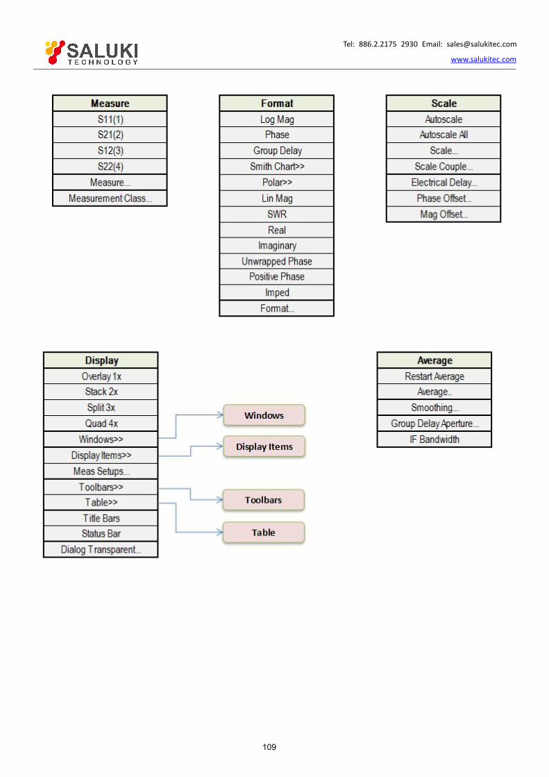
5. Menu....................................................................................................................................................................................... 1065.1. Menu structure...............................................................................................................................................................1065.2. Description of menu....................................................................................................................................................... 113
6. Measurement Optimization........................................................................................................................................................1666.1. Reduction of Accessory Influence....................................................................................................................................1666.2. Improvement of Reflection Accuracy of Low-loss 2-port Device......................................................................................... 1676.3. Increase of Dynamic Range............................................................................................................................................1696.4. Improvement of Measurement Results of Electrical Long Device....................................................................................... 1716.5. Improvement of Phase Measurement Accuracy................................................................................................................1726.6. Reduction of trace Noise................................................................................................................................................ 1786.7. Increase of Data Point Number....................................................................................................................................... 1816.8. Improvement of Measurement Stability............................................................................................................................1826.9. Increase of sweep Speed............................................................................................................................................... 184

Tel: 886.2.2175 2930 Email: [email protected]
www.salukitec.com
5
6.10. Improvement of Efficiency of Multi-state Measurement....................................................................................................1876.11. Rapid Data Transmission..............................................................................................................................................1886.12. Use of Macro............................................................................................................................................................... 189
7. Calibration................................................................................................................................................................................1927.1. Calibration Overview......................................................................................................................................................1927.2. Selection of Calibration Type...........................................................................................................................................1937.3. Calibration Guide...........................................................................................................................................................1957.4. High-accuracy Measurement Calibration..........................................................................................................................1987.5. Measurement Errors...................................................................................................................................................... 1997.6. Editing of Calibration Kit Definition...................................................................................................................................2027.7. 7.7 Standard Calibration Kit............................................................................................................................................ 2107.8. TRL Calibration..............................................................................................................................................................2127.9. Fixture Compensation Calibration................................................................................................................................... 2137.10. Electronic Calibration................................................................................................................................................... 221
8. Basis of Network Measurement................................................................................................................................................. 2258.1. Reflection Measurement.................................................................................................................................................2258.2. Phase Measurement......................................................................................................................................................2278.3. Amplifier Parameter Specifications..................................................................................................................................2298.4. Complex Impedance...................................................................................................................................................... 2318.5. Group Delay..................................................................................................................................................................2338.6. Absolute Output Power...................................................................................................................................................2368.7. AM-PM Transformation...................................................................................................................................................2378.8. Linear phase offset.........................................................................................................................................................2408.9. Reverse Isolation...........................................................................................................................................................2418.10. Small Signal Gain and Flatness.....................................................................................................................................242
9. Remote control.........................................................................................................................................................................2459.1. Basis of Remote Control.................................................................................................................................................2459.2. Programmed Port and Configuration of Instrument........................................................................................................... 2599.3. Basic Programming Method of VISA Interface..................................................................................................................2619.4. I/O Library..................................................................................................................................................................... 269
10. Fault Diagnoses and Repair.....................................................................................................................................................27210.1. Operating principle.......................................................................................................................................................27210.2. Fault Diagnosis and Troubleshooting.............................................................................................................................27310.3. Error Information..........................................................................................................................................................275
11. Technical Indicators and Measurement Methods....................................................................................................................... 29111.1. Technical Indicators......................................................................................................................................................29111.2. Measurement Methods.................................................................................................................................................298

Tel: 886.2.2175 2930 Email: [email protected]
www.salukitec.com
6
1. Manual GuideThis chapter summarizes the functions, structure and main contents of the user manual of S3602 vector network analyzers, and therelated documents for the user.
About manual
Related documents
1.1.About the Manual
The manual describes the purposes, performance indicators, basic operating theory, operating method, operation precautions, etc. ofS3602 vector network analyzers produced by Saluki Technology, to help you rapidly get familiar with and understand key points of theinstrument operation and use. Please read this User Manual carefully and follow its guidance.
Due to the limit of time and knowledge of the writer, there may be some omissions or errors, and you are welcome to correct any sucherrors. We are sorry for the flaws which may cause your inconvenience.
The user manual includes the following chapters.
Overview
The chapter provides an overview of the characteristics and operation precautions of S3602 vector network analyzers, mainly including aproduct overview and a safe operation guide.
Introduction
This chapter describes the preparations before operation of S3602 vector network analyzers, routine maintenance of the system andinstrument, overview of the front panel and the rear panel, operation interface, analyzer menus, tracks, channels, windows, and analysisand saving of measurement data.
Measurement setups
This chapter describes various settings of the network analyzer in operation, including resetting of the analyzer, selection ofmeasurement parameters, setting of the frequency range, setting of the signal power level, setting of sweep, selection of the trigger mode,selection of the data format and scale, viewing of several tracks, opening of several channels, and setting of the analyzer display.
Menu
This chapter describes the menu structure and items according to functional categories to facilitate query and reference.
Measurement optimization
This chapter describes how to optimize the measurement accuracy by means of proper settings, including reduction of accessoryimpacts, improvement of the reflection accuracy of the low-loss 2-port device, increase of the dynamic range, improvement of themeasurement results of the electrical length and the measurement accuracy of the phase, reduction of the trace noise and receivercrosstalk, increase of data points, improvement of the measurement stability, sweep speed, multi-status measurement efficiency andrapid data transmission, use of macros, etc.
Calibration
This chapter introduces the calibration type and method of S3602 vector network analyzers to improve the accuracy of measurement.
Network measurement basics
Tel: 886.2.2175 2930 Email: [email protected]
www.salukitec.com
7
This chapter describes the basic concepts and related theories of senior network parameter measurement.
Remote control
This section outlines the remote control of the instrument, so that the user can rapidly get to know how to remotely control the instrument.It is divided into four sections: the program control basics describe the concepts related to program control, software configuration,program-controlled port, SCPI commands, etc.; instrument port configuration describes the connection and software configuration of theprogram-controlled port of S3602 vector network analyzers; basic programming of VISA interface provides an example of basicprogramming with text illustration and example codes, so that the user can rapidly get to know the programming method; and I/O functionlibrary describes the basic concepts of the instrument drive and the basic installation and configuration requirements of theIVI-COM/IVI-C drive.
Fault diagnosis and repair
This section describes the overall operating theory, fault diagnosis and troubleshooting, and errors and repair.
Technical indicators and test methods
This section describes the main technical indicators of S3602 analyzers and the recommended test instructions for the user.
1.2.Related Documents
The documents related to S3602 series vector network analyzer include:
User Manual
Program control document
Quick Start Guide
User ManualThis manual introduces the functions and operation methods of the instrument in details, including configuration, measurement, programcontrol, maintenance, etc. It aims to guide the user to comprehensively understand the functional characteristics and common testmethods of the instrument. It mainly includes the following chapters:
Manual Navigation
Overview
Introduction
Measurement setups
Menu
Measurement optimization
Calibration
Network measurement basics
Remote control
Fault diagnosis and repair
Technical indicators and measurement method

Tel: 886.2.2175 2930 Email: [email protected]
www.salukitec.com
8
Program control documentThis manual introduces the remote programming basis, SCPI basis, SCPI commands, programming examples, I/O drive function library,etc. It aims to guide the user to rapidly and comprehensively know the program control commands and methods of the instrument. Itmainly includes the following chapters:
Remote control
Program control commands
Programming examples
Error illustration
Appendix
Quick Start GuideThis manual introduces the basic operations of configuration, start-up and measurement of the instrument, aiming to help the user rapidlyknow the characteristics of the instrument and understand basic settings and operations. It mainly includes the following chapters:
Preparation for use
Typical application
Help

Tel: 886.2.2175 2930 Email: [email protected]
www.salukitec.com
9
2. OverviewThis chapter describes the main performance characteristics, purposes and technical indicators of S3602analyzers. It also includes theprecautions for proper operation, electrical safety, etc.
Product overview
Safe operation guide
2.1.Product Overview
S3602 series vector network analyzer is a new generation of vector network analyzer, launched by Saluki Technology. In the hardware,new design concept and technical architecture are adopted, thus significantly improving key technical performance indicators such as theoverall scanning speed and dynamic range. In the software, the embedded computer with high-performance microprocessor chip andplatform environment based on Windows7 operating system are applied, thus greatly improving the overall interconnection and usability.
S3602 series vector network analyzers have multiple calibration modes such as frequency response, single port, response isolation,enhanced response, double ports and electrical calibration, and multiple display modes such as the logarithmic amplitude, linearityamplitude, standing wave, phase, group delay and Smith chart. It is equipped with various standard interfaces, such as USB, LAN, GPIBand VGA. In addition to all measurement functions of the traditional vector network analyzer, the instrument can be used to testcomprehensive parameters of multiple functions such as the mixer/converter, active intermodulation distortion and harmonic distortion,gain compression and two-dimensional sweep and S-parameter of the pulse network, and accurately measure the amplitude frequencycharacteristics, phase frequency characteristics and group delay characteristics of the microwave network.
The instrument can be widely applied in measurement of the transmission/reception (T/R) module, dielectric material properties,microwave pulse characteristics and photoelectric properties. It is an indispensable tester in research and production of the phased arrayradar, communication, RF microwave device and other systems.
Product Features: 12.1-inch high-resolution touch screen;
Multiple calibration modes such as the frequency response, single port, frequency isolation, double ports, TRL and electricalcalibration;
16 display windows capable of displaying 8 traces at the same time, and 64 independent measurement channels to rapidlyimplement complex test solutions;
Record/run (one-button operation), greatly simplifying the Measurement setups steps and improving the working efficiency;
Multiple display formats such as the logarithmic amplitude, linearity amplitude, standing wave, phase, group delay, Smith chart andpolar coordinates;
USB, GPIB, LAN and VGA interface;
Two options: single-source stimulus type 2-port vector network analyzer and double-source stimulus
type four-port vector network analyzer;
Multiple functions such as the pulse measurement, time domain measurement, mixer measurement, active intermodulationdistortion measurement, gain compression and two-dimensional scanning measurement, millimeter wave spreading, antenna andRCS measurement reception.
1.Simple and intuitive humane user interface, facilitating operation and improving the test efficiency.
Tel: 886.2.2175 2930 Email: [email protected]
www.salukitec.com
10
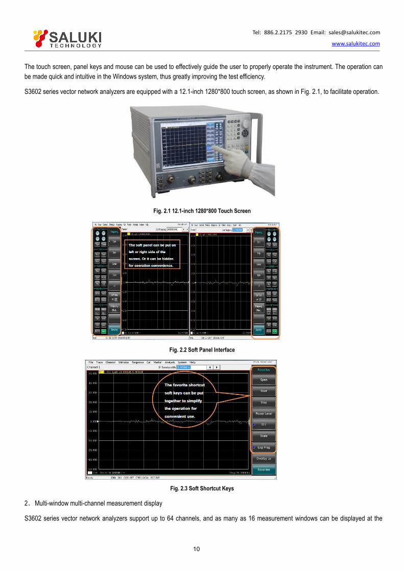
The touch screen, panel keys and mouse can be used to effectively guide the user to properly operate the instrument. The operation canbe made quick and intuitive in the Windows system, thus greatly improving the test efficiency.
S3602 series vector network analyzers are equipped with a 12.1-inch 1280*800 touch screen, as shown in Fig. 2.1, to facilitate operation.
Fig. 2.1 12.1-inch 1280*800 Touch Screen
Fig. 2.2 Soft Panel Interface
Fig. 2.3 Soft Shortcut Keys
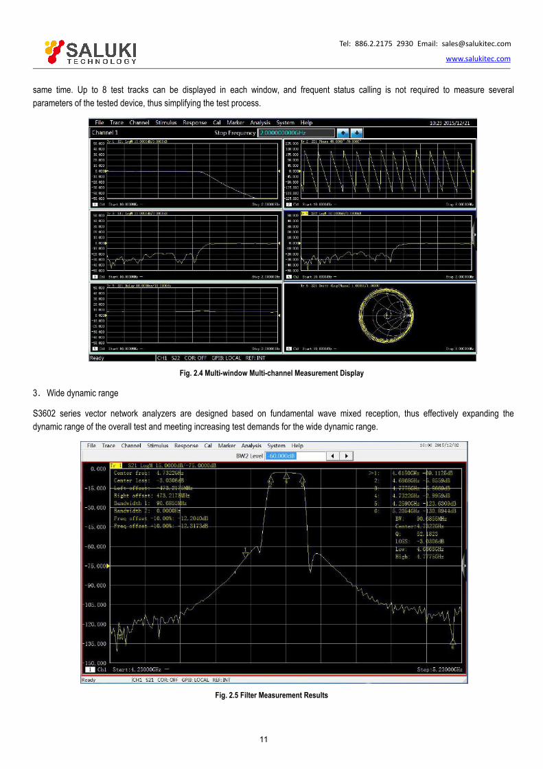
2.Multi-window multi-channel measurement display
S3602 series vector network analyzers support up to 64 channels, and as many as 16 measurement windows can be displayed at the
Tel: 886.2.2175 2930 Email: [email protected]
www.salukitec.com
11
same time. Up to 8 test tracks can be displayed in each window, and frequent status calling is not required to measure severalparameters of the tested device, thus simplifying the test process.
Fig. 2.4 Multi-window Multi-channel Measurement Display
3.Wide dynamic range
S3602 series vector network analyzers are designed based on fundamental wave mixed reception, thus effectively expanding thedynamic range of the overall test and meeting increasing test demands for the wide dynamic range.
Fig. 2.5 Filter Measurement Results

Tel: 886.2.2175 2930 Email: [email protected]
www.salukitec.com
12
4.Automatic test
The automatic test can help to save a lot of time and effectively reduce the test cost in a flexible automation environment.
The vector network analyzer is controlled with SCPI commands to complete automatic tests.
Codes are directly executed from the vector network analyzer or external PC through a LAN or GPIB interface.
The application program can be directly run in the instrument, with no external PC.
Fig. 2.6 Automatic Test
1) GPIB interface
S3602 series vector network analyzers are equipped with a 24-pin D-type female GPIB connector, which conforms to the IEEE-488standard and is used to send and receive GPIB/SCPI commands.
2) USB Interface
S3602 series vector network analyzers are equipped with nine high-speed USB interfaces (eight A-type interfaces and one B-typeinterface) to facilitate the connection to the keyboard, mouse, printer, electronic calibrator and other peripherals with USB interfaces.
3) Printing function
S3602 series vector network analyzers have a powerful printing function, and are able to output or print the contents of the measurementdisplay into a specified file through a printer. A local or network printer with a LAN or USB interface can be used. Measurement resultscan be printed after the printer is added to the Windows 7 operating system.
2.2.Safety GuidePlease carefully read and strictly follow the notes for attention below!
We will spare no effort to ensure that all production stages conform to the latest safety standards to guarantee the highest safety forusers. The design and test of our product and ancillary equipment thereof have been up to relevant standards of security; qualityassurance system has been established to monitor the product quality to ensure the consistency with such standards. Precautionsproposed in this User Manual should be followed to keep equipment intact and operations safe. Please do not hesitate to consult us ifyou have any questions.
Tel: 886.2.2175 2930 Email: [email protected]
www.salukitec.com
13
However, it is your responsibility to operate the product in a correct way. Please read and follow the safety instructions carefully beforeoperating the instrument. The instrument is applicable to the industrial and laboratory environment or field measurement. Pay attention tothe limitations for proper operation to avoid personal injury or property damage. We will not take any responsibility for any misuse orinconsistency as required, and you are liable for any risks incurred by. Therefore follow the safety instructions to prevent from personalinjury or property damage. Please keep the basic safety instructions and product documentation safe and submit them to end users.
Safety signs
Operation status and location
Power safety
Operation precautions
Maintenance
Battery and power supply module
Transportation
Waste disposal/environment protection
2.2.1. Safety Signs
2.2.1.1. Product-related Signs
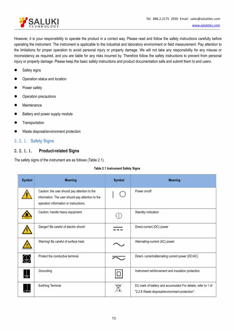
The safety signs of the instrument are as follows (Table 2.1).
Table 2.1 Instrument Safety Signs
Symbol Meaning Symbol Meaning
Caution: the user should pay attention to theinformation. The user should pay attention to theoperation information or instructions.
Power on/off
Caution: handle heavy equipment. Standby indication
Danger! Be careful of electric shock! Direct-current (DC) power
Warning! Be careful of surface heat. Alternating-current (AC) power
Protect the conductive terminal. Direct- current/alternating current power (DC/AC)
Grounding Instrument reinforcement and insulation protection.
Earthing Terminal EU mark of battery and accumulator.For details, refer to 1 of"2.2.8 Waste disposal/environment protection".

Tel: 886.2.2175 2930 Email: [email protected]
www.salukitec.com
14
Caution: electrostatic sensitive device. Be careful. EU mark for electronic parts to be collected separately Fordetails, refer to 2 of "2.2.8 Waste disposal/environmentprotection".
Warning! Radiation. For details, refer to 7 of 2.2.4"Operation Precautions" of this section.
2.2.1.2. Manual-related Signs
The following safety warning signs are used in the product manual to remind the user to operate the instrument safely and pay attentionto relevant information.
Danger sign: personal injury and equipment damage may be caused if no attention is paid.
Warning sign: personal injury and equipment damage may be caused if no attention is paid.
Caution sign: minor or moderate personal injury and equipment damage may be caused if no attention is paid.
Attention sign: it indicates important prompts but no danger.
Prompt sign: information of the instruction and operation.
2.2.2. Operation Status and Location
Pay attention to the following items before operation:
1) Unless otherwise stated, S3602 series vector network analyzers should be placed steadily and operated indoor with protection of IP2X. The maximum altitude must not exceed 2,000m in operation and 4,500m in transportation. The actual power supply voltagemay be the indicated voltage ± 10%, and the power supply frequency may be the indicated frequency ± 5%. Both the overvoltageprotection and the pollution intensity are Class 2.
2) Do not place the instrument on a wet surface, vehicle, cabinet, table and other objects which are not fixed and do not conform to theload conditions. Place the instrument steadily and fix it on the solid object surface (such as the anti-static workbench).
3) Do not place the instrument on a heat dissipating surface (such as a radiator). The operating temperature must not exceed thespecified range of relevant indicators of the instrument. Overheating may result in electric shock, fire, etc.
Tel: 886.2.2175 2930 Email: [email protected]
www.salukitec.com
15
2.2.3. Power Safety
Precautions for the power supply of the instrument:
1) Ensure that the actual power supply voltage is the same as that marked on the instrument before powering-on. If the power supplyvoltage is changed, replace the fuse of the instrument.
2) Refer to the power supply requirements on the rear panel of the instrument. Use three-core power cords. Ensure that the powercord is grounded reliably. Floating or improper grounding may result in damage to the instrument and even operator injuries.
3) Do not damage the power cord; otherwise, electrical leakage may be caused, resulting in instrument damage and even operatorinjuries. If any, check the external power cord or terminal block before operation to ensure the power safety.
4) If the power socket is not equipped with any ON/OFF switch, the power plug can be directly pulled off to power off the instrument. Inthis case, ensure it is easy to plug and unplug the power line.
5) Do not use any damaged power cord. Before connecting the power cord to the instrument, check the power cord for integrity andsafety. Reasonably place the power cord to avoid the impact from human activities. For example, the operator may fall over if thepower cord extends over long distances.
6) The TN/TT power network is required. The maximum rated current of the fuse should be 16A (contact the manufacturer if a fuse ofhigher current is required).
7) Keep the socket clean and the plug and the socket in good and firm contact.
8) The socket and power cord must not be overloaded; otherwise, fire or electric shock may be caused.
9) If the voltage Vrms is higher than 30V in the test, take appropriate protective measures (such as use of the appropriate testinstrument and fuse, limitation of the current, electrical isolation and insulation, etc.) to avoid damage to the instrument.
10) The instrument shall conform to IEC60950-1/EN60950-1 or IEC61010-1/EN61010-1 so as to realize the connection to a PC orindustrial personal computer.
11) Unless specially permitted, the instrument shell must not be opened; otherwise, internal circuits and parts may be exposed,resulting in unnecessary damage.
12) If the instrument needs to be fixed in a test place, the protective ground wire should be installed between the test place andinstrument by the electrician with qualifications.
13) Take appropriate overload protection measures to avoid instrument damages or personal injuries caused by overload voltage(arising from lightning, etc.).
14) If the instrument shell is opened, unnecessary parts must not be placed into the shell; otherwise, short circuiting, instrumentdamages and even personal injuries may be caused.
15) Unless otherwise stated, the instrument is not subject to waterproof protection. Therefore, the instrument must not contact withliquid to prevent damages and even personal injuries.
16) The instrument must not be placed in a place where mist can be easily produced. For example, if the instrument is handled in anenvironment with temperature fluctuation, hazards such as electric shock may be caused by water drops produced on theinstrument.

Tel: 886.2.2175 2930 Email: [email protected]
www.salukitec.com
16
2.2.4. Operation Precautions
1) The instrument operator must have certain professional and technological knowledge, good psychological quality and emergencyresponse capability.
2) Refer to relevant requirements in "2.2.7 Transportation" before handling or transporting the instrument.
3) Allergic substances (such as nickel) are produced inevitably during instrument production. If the operator shows any allergicsymptom (such as rash, frequent sneezing, red eye, breathing difficulty, etc.), immediately seek medical help to eliminate thesymptoms.
4) Refer to relevant requirements in "2.2.8 Waste disposal/environmental protection" of this section before removing and disposal ofthe instrument.
5) RF instruments may result in high-intensity electromagnetic radiation. The pregnant women and operators with heart pacemakermust be protected particularly. If the degree of radiation is high, take appropriate measures to remove the radiation source so as toprevent personal injury.
6) If a fire occurs, toxic substances will be released by the damaged instrument. In this case, the operator should wear appropriateprotective equipment (such as the protective mask and clothing) for protection.
7) The laser product should be marked with warnings according to the laser category, as personal injuries may be caused as a resultof laser radiation and high electromagnetic power of such products. 8) If the instrument is integrated with any laser product (such asa CD/DVD drive), no additional function should be added, except the settings and functions described in the manual, in order toprevent personal injuries caused by laser beams.
8) The electromagnetic compatibility should conform to the EN55011/CISPR11, EN55022/CISPR22 and EN55032/CISPR32standards.
Class A equipment:
applicable to any place except in residential areas and a low-voltage power supply environment.
Note: Class A equipment is suitable for the industrial operating environment. As wireless communication disturbance may be caused toresidential areas, the operator should take appropriate measures to reduce disturbance.
Class B equipment:
It is applicable to the residential area and low-voltage power supply environment.
2.2.5. Maintenance
1) The instrument chassis must be opened by an authorized operator who has received special technical training. The power cordshould be disconnected before operation, so as to avoid instrument damages and even personal injuries.
2) The instrument should be repaired, replaced and maintained by special electronic engineers of the manufacturer, and the replacedor maintained parts must be subject to safety tests to ensure the safety of subsequent operation.
2.2.6. Battery and Power Supply Module
Carefully read relevant information before using the battery and power supply module, so as to avoid explosion, fire and even personalinjuries. In some cases, waste alkaline batteries (such as lithium batteries) should be disposed in accordance with the EN62133 standard.Precautions for battery use:
1) Do not damage the battery.
Tel: 886.2.2175 2930 Email: [email protected]
www.salukitec.com
17
2) The battery and power supply module must not be exposed to flame and other heat sources. They must be prevented from directsunlight and should be kept clean and dry in storage. Clean the connection port of the battery or power supply module with cleanand dry soft cloth.
3) Do not make the battery or power supply module short-circuited. As the short circuit may be easily caused by mutual contact orcontact with other conductors, several batteries or power supply modules must not be stored in the same carton or drawer. Do notremove the original package until the battery and power supply module are required.
4) The battery and power supply module must be prevented from mechanical impact.
5) The leaky battery must not contact with the skin or eyes. In case of contact, rinse with plenty of clean water and immediately seekmedical help.
6) Use the standard battery and power supply module provided by the manufacturer. Any improper replacement or charging of alkalinebatteries (such as lithium batteries) may easily result in explosion.
7) The waste battery and power supply module should be recovered and disposed separately with other wastes. The battery containstoxic substances. It must be discarded or recycled according to the local provisions.
2.2.7. Transportation
1) The heavy instrument must be handled carefully. If necessary, use tools (such as the crane) to move the instrument to preventdamage to the body.
2) The instrument handle is applicable to handling by individuals. The instrument must not be fixed on the transport equipment duringtransportation. In order to prevent damage to the property and body, observe the manufacturer‘s safety provisions on instrumenttransportation.
3) If the instrument is operated on the transport vehicle, the driver should drive carefully to ensure the transportation safety. Themanufacturer will not be responsible for emergencies in transportation. Do not operate the machine during transportation. Takereinforcement and protection measures to ensure the safety of transportation.
2.2.8. Waste Disposal/Environmental Protection
1) Do not dispose the equipment with the battery or accumulator mark along with other unclassified wastes. Instead, such equipmentshould be collected separately and discarded or disposed in the appropriate collection place or by the customer service center ofthe manufacturer.
2) Do not dispose the discarded electronic equipment with other unclassified wastes. Such electronic equipment should be collectedseparately. The manufacturer has the right and responsibility to help end users to dispose waste products. If necessary, contact thecustomer service center of the manufacturer for corresponding disposal to avoid damage to the environment.
3) Toxic substances (heavy dust such as lead, beryllium, nickel, etc.) may be released in machining or thermal reprocessing of theinstrument or internal parts. In this case, the instrument or internal parts must be removed by technical personnel who havereceived special training and relevant experience, so as to avoid personal injuries.
4) Toxic substances or fuel released by the instrument in reprocessing should be disposed in the specified method, with reference tothe safety operation rules put forward by the manufacturer, so as to avoid personal injuries.
Tel: 886.2.2175 2930 Email: [email protected]
www.salukitec.com
18
3. Introduction to UseThis chapter introduces the operation precautions, front and rear panel browsing, commonly used basic measurement methods, data filemanagement, etc. of S3602 series vector network analyzers, so that the user has a preliminary understanding of the instrument andmeasurement process.
Preparation before use
Front and rear panel
Analyzer interface
Analyzer trace, channel and window
Analysis data
Data output
3.1.Preparation before Use Pre-operation preparation
System recovery and installation procedures of analyzer
Routine maintenance
3.1.1. Pre-operation Preparation
This chapter introduces the precautions for initial setting and operation of S3602 series vector network analyzer.
Prevent damage to the instrument.
In order to avoid electric shock, fire and personal injury:
Do not open the casing without permission.
Do not disassemble or modify any part which is not described in this manual. Disassembly may result in declining of theelectromagnetic shielding performance, damage to parts in the instrument, etc., thus affecting the product reliability. In this case, wewill not provide free maintenance services even within the warranty period.
Carefully read the relevant contents in "2.2 Safe Operation Guide" of this manual, and the safety precautions listed below. At thesame time, pay attention to the specific operating environment requirements on the page of data.
Electrostatic protection
Pay attention to anti-static measures in the workplace to prevent damage to the instrument. For details, refer to the relevant contents of“2.2 Safe Operation Guide" of this manual.

Tel: 886.2.2175 2930 Email: [email protected]
www.salukitec.com
19
Pay attention to the following requirements before operation:
The improper operation location or Measurement setups may result in damage to the instrument or the connected instrument. Payattention to the following requirements before powering on the instrument:
The fan blades and ventilation holes are not blocked, and the instrument is at least 10cm away from the wall.
Keep the instrument dry.
Horizontally and reasonably arrange the instrument.
The ambient temperature meets the requirements on the page of data.
The input signal power of the port is within the specified range.
The signal output port is properly connected and not overloaded.
Influence of electromagnetic interference (EMI):
Electromagnetic interference will affect measurement results, therefore:
Select the appropriate shielded cable. Example: use the dual-shielded radio-frequency/network connection cable.
Please promptly close the cable connection port which is open and not used temporarily or the connection port connected to thematching load.
Refer to the electromagnetic compatibility (EMC) level on the data page.
3.1.1.1. Unpacking
1) Appearance inspection
Step 1: check whether the outer packing box and shockproof package are damaged. In case of any damage, keep the outer package forfuture use. Continue inspection according to the following steps.
Step 2: unpack the box and check whether the host and accompanying articles are damaged.
Step 3: carefully check the above articles according to Table 3.1.
Step 4: Do not turn on the power supply of the instrument if the outer package, instrument and accompanying article is damaged or anyerror exists. Contact our service consultation center at the service consultation hotline on the cover. We will rapidly repair or replace theinstrument, depending on the actual situation.
The heavy instrument and packing box must be handled by two persons and placed carefully.
2) Packing Check

Tel: 886.2.2175 2930 Email: [email protected]
www.salukitec.com
20
Table 3.1 List of Accompanying Articles of S3602
Description Qty. Function
Main Machine
S3602 Series VNA 1
Standard Accessories 1
Power cord 1
USB Keyboard/mouse 1
User Manual 1
Packing list 1
Warranty 1
Options
201 1 2-ports, single source, with extended power range
400 1 4-ports, dual source, base configuration
401 1 4-ports, dual source, with extended power range
402 1 Intermodulation distortion application
008 1 Pulsed RF Measurements
S10 1 Time Domain Measurement
S80 1 Frequency offset measurements
S82 1 Scalar calibrated converter measurements
S83 1 Vector and scalar calibrated converter measurements
S84 1 Embedded LO measurements
S86 1 Gain compression application
S3602 A/B Options
SAV31121 Calibration Kit 1 Calibration
FB0HA0HC025.0 1 3.5mm test cable
FB0HA0HB025.0 1 3.5mm test cable
S3602 C Options
SAV31123 Calibration Kit 1 Calibration
FE0BN0BM025.0 1 2.4mm test cable
Tel: 886.2.2175 2930 Email: [email protected]
www.salukitec.com
21
Description Qty. Function
FE0BN0BL025.0 1 2.4mm test cable
S3602 D Options
SAV31123A Calibration Kit 1 Calibration
FE0BN0BM025.0 1 2.4mm test cable
FE0BN0BL025.0 1 2.4mm test cable
S3602 E Options
SAV31128 Calibration Kit 1 Calibration
FF0CN0CM025.0 1 1.85mm test cable
FF0CN0CL025.0 1 1.85mm test cable
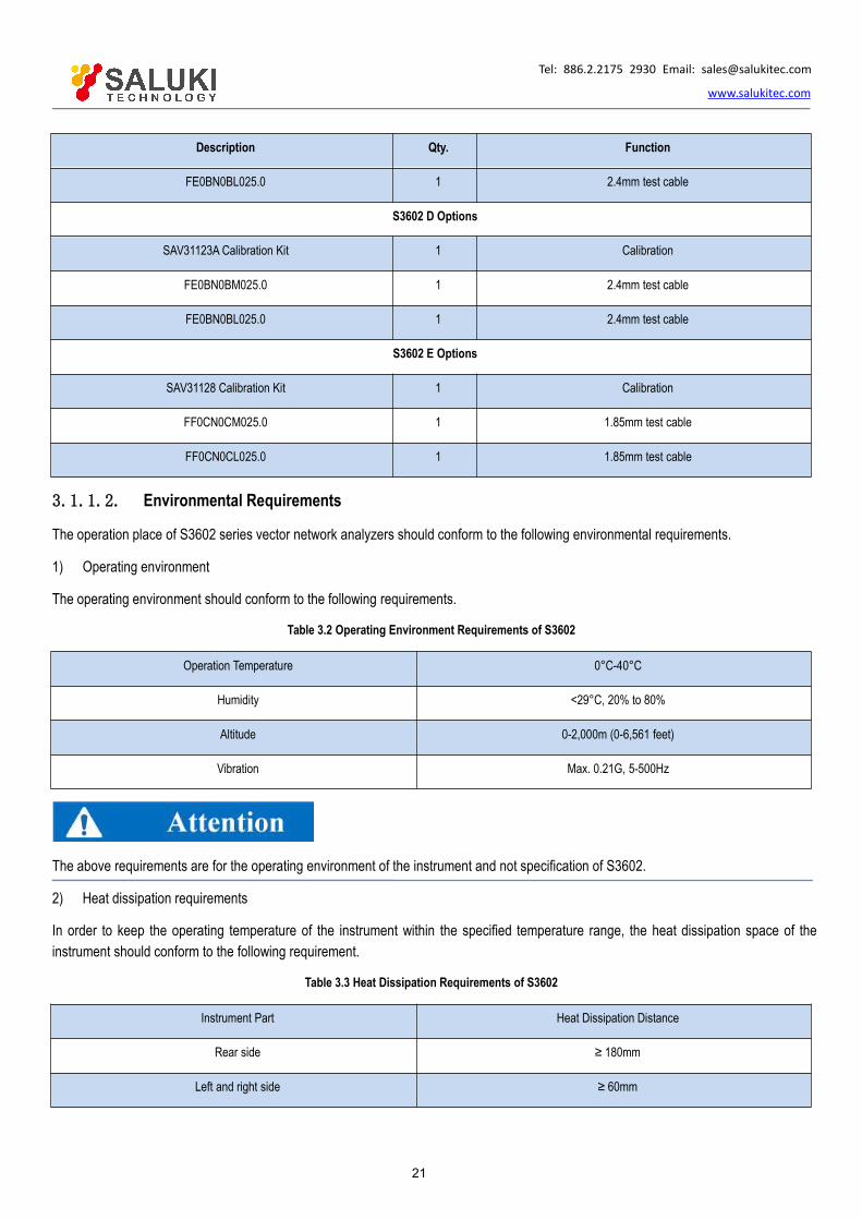
3.1.1.2. Environmental Requirements
The operation place of S3602 series vector network analyzers should conform to the following environmental requirements.
1) Operating environment
The operating environment should conform to the following requirements.
Table 3.2 Operating Environment Requirements of S3602
Operation Temperature 0°C-40°C
Humidity <29°C, 20% to 80%
Altitude 0-2,000m (0-6,561 feet)
Vibration Max. 0.21G, 5-500Hz
The above requirements are for the operating environment of the instrument and not specification of S3602.
2) Heat dissipation requirements
In order to keep the operating temperature of the instrument within the specified temperature range, the heat dissipation space of theinstrument should conform to the following requirement.
Table 3.3 Heat Dissipation Requirements of S3602
Instrument Part Heat Dissipation Distance
Rear side ≥ 180mm
Left and right side ≥ 60mm
Tel: 886.2.2175 2930 Email: [email protected]
www.salukitec.com
22
3) Electrostatic protection
Static electricity is destructive to electronic components and devices. Generally, two anti-static measures can be taken: combination ofconductive table mat and wrist strap; and combination of conductive floor mat and ankle strap. Anti-static effect will be better when twomeasures are used at the same time. If used independently, only the former can make sure the safety. In order to ensure the user safety,the ground isolation resistance of anti-static components must be 1MΩ at least.
The follow anti-static measures should be taken to reduce static damage:
All instruments must be properly grounded to prevent static electricity.
The internal and external conductor of the cable should respectively contact with the ground temporarily before the coaxial cableand instrument are connected.
Workers must wear the anti-static wrist strap or take other anti-static measures before contact with the connector or wire or anyassembly.
Voltage range
The above anti-static measures are not suitable for the places with the voltage higher than 500V.
3.1.1.3. On/Off
1) Precautions before powering-on
Check the following items before powering on the instrument.
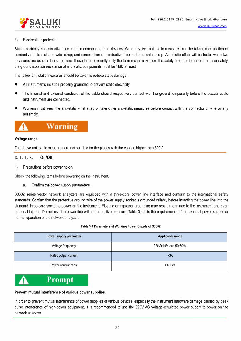
a. Confirm the power supply parameters.
S3602 series vector network analyzers are equipped with a three-core power line interface and conform to the international safetystandards. Confirm that the protective ground wire of the power supply socket is grounded reliably before inserting the power line into thestandard three-core socket to power on the instrument. Floating or improper grounding may result in damage to the instrument and evenpersonal injuries. Do not use the power line with no protective measure. Table 3.4 lists the requirements of the external power supply fornormal operation of the network analyzer.
Table 3.4 Parameters of Working Power Supply of S3602
Power supply parameter Applicable range
Voltage,frequency 220V±10% and 50-60Hz
Rated output current >3A
Power consumption >600W
Prevent mutual interference of various power supplies.
In order to prevent mutual interference of power supplies of various devices, especially the instrument hardware damage caused by peakpulse interference of high-power equipment, it is recommended to use the 220V AC voltage-regulated power supply to power on thenetwork analyzer.

Tel: 886.2.2175 2930 Email: [email protected]
www.salukitec.com
23
b. Confirm and connect the power line.
S3602 series vector network analyzers are equipped with the three-core power line interface and conform to national safety standards.Confirm that the protective ground wire of the power line of the network analyzer is reliably grounded before powering on the networkanalyzer. Floating or improper grounding may result in instrument damage and even operator injuries. Do not use the power line with noprotective ground wire. When the appropriate power socket is connected, the instrument shell will be grounded through the power line.The rated voltage of the power line should be no less than 250V, and the rated current should be no less than 6A.
Connection of the power line to the instrument:
Step 1: confirm that the power line is not damaged.
Step 2: connect the power socket on the rear panel of the instrument to the well grounded three-core power socket through the powerline.
Grounding
Improper/wrong ground might lead to instrument destroy or even personal injury. Ensure that the protective ground wire and the groundwire of the power supply are in good contact before powering-on to start the network analyzer.
Use the power socket with protective ground wire. Do not use the external cable, power line or autotransformer subject to no groundingprotection instead of the protective ground wire. If required, connect the common end of the autotransformer to the protective ground wireof the power connector.
2) Initial power-on
The method and precautions of initial power-on are as follows.
a) Connection of power supply
Check the power supply parameters and power cord before initial powering-on. For details, refer to the precautions before powering-on in3.1.1.3 of the user manual.
Step 1: connect the power line. Connect one end of the supporting power line of the network analyzer or the three-core power lineconforming to the requirements in the packing box to the power socket (as shown in Fig. 3.1) on the rear panel of the network analyzer.The voltage indicator of the network analyzer is marked beside the power socket to remind the user that the applied voltage shouldconform to the requirements. Connect the other end of the power cord to the required AC power supply.
Step 2: turn on the power switch on the rear panel. As shown in Fig. 3.2, check whether the standby indicator above the power switch onthe front panel (as shown in Fig. 3.3) is ON and yellow.
Step 3: turn on the power switch on the front panel, as shown in Fig. 3.3. Do not connect any device to the network analyzer beforestart-up. Start the instrument under normal conditions. After start-up, the indicator above the power switch on the front panel will turngreen.
Fig. 3.1 S3602 Power Socket (Left)
Tel: 886.2.2175 2930 Email: [email protected]
www.salukitec.com
24
Fig. 3.2 Switch on Rear Panel (Middle)
Fig. 3.3 Power Switch on Front Panel (Right)
b) Turn on/off
Start-up
Step 1: turn on the power switch (“|") on the rear panel.
Step 2: turn on the power switch in the lower left corner of the front panel. Check whether it is pressed ( ). In this case, the powerindicator above the power switch will turn green from yellow.
Step 3: about one minute is required for the network analyzer to start the Windows 7 system. After a series of self-inspection andadjustment procedures, the main measurement program will be run.
Preheating for cold start of the instrument
In order to meet the performance indicators of S3602 series vector network analyzer in cold start, preheat it more than 30 minutes beforemeasurement.
Run the analyzer application program.
The application program will be automatically run after the network analyzer is started. After exiting the application program, you can runthe measurement program again according to the following method.
Method 1: click [Start] of the task bar in the lower left corner of the screen. Point to [Program] in the Start menu and then [Vector networkanalyzer] in the program sub-menu. Click [Vector network analyzer] in the pop-up sub-menu. Then the measurement application programwill be run in the analyzer. You can also double-click the shortcut key on the desktop to run the program.
Method 2: press [Reset] in the functional key zone. Then the application program of the S3602 series vector network analyzer will berun.
Shutdown
Step 1: turn off the power switch in the lower left corner of the front panel (as shown in Fig. 3.3). In this case, the shutdown process isstarted (the power supply will be shut down after processing of software and hardware). After dozens of seconds, the instrument will bepowered off. The power indicator above the power switch will turn yellow from green.
Step 2: turn off the power switch ("O") on the rear panel, or disconnect the power supply of the instrument.
Thus the instrument is off.
Shut Down
The instrument in normal operation must be shut down by operating the power switch of the front panel. Do not directly operate thepower switch of the rear panel or directly cut off the power supply of the instrument; otherwise, the instrument cannot be shut downnormally and may be damaged, or the current status/measurement data may be lost. Shut down the instrument properly. In case offailure of normal shutdown caused by the anomaly of the operating system or application program, hold [Power/Standby] key for fourseconds at least to shut down the analyzer.

Tel: 886.2.2175 2930 Email: [email protected]
www.salukitec.com
25
c. Cutoff of power supply
In order to prevent personal injury under abnormal conditions, the power supply of the network analyzer requires emergency cutoff. Inthis case, pull off the power cord (from the AC power socket or the power socket of the rear panel of the instrument). Therefore, sufficientoperating space should be reserved for direct cutoff of the power supply if necessary.
3.1.1.4. Proper Use of Connector
The connector is always required in various tests of the network analyzer. Although the connectors of the calibrator, test cable andanalyzer measurement port are designed and manufactured according to the highest standards, the service life is limited. Inevitable wearin normal operation may result in declining of performance indicators of the connector and failure to meet measurement requirements.Proper connection of the connector in maintenance and measurement can help to obtain accurate and repeatable results, prolong theservice life of the connector, and reduce the measurement cost. Pay attention to the following items in actual operation.
1.Inspection of connector
Wear the anti-state wristband in connector inspection. It is recommended to use the magnifying lens to check the following items.
1) Check whether the plating surface is worn or deeply scratched.
2) Check whether threads are deformed.
3) Check whether there are metal particles on the connector threads and joint surfaces.
4) Check whether the internal conductor is bent or cracking.
5) Check whether the connector screw is tightened properly.
Prevent damage to the instrument port in connector inspection.
Any damaged connector may result in damage to the connector in good conditions even in the first measurement connection. In order toprotect each interface of the network analyzer, the connector must be checked before connection.
2.Cleaning of connector
Wear the anti-static wrist strap before cleaning the connector. Clean the connector according to the following steps.
1) Remove loose particles on the connector threads and joint plane with clean low-pressure air. Thoroughly check the connector. Ifrequired, further clean the connector according to the following steps.
2) Soak the lint-free cotton swab with isopropyl alcohol (not thoroughly soaked).
3) Clean the dirt and debris on the joint plane and threads of the connector with the swab. Do not apply force on the internal conductorat the center during cleaning of the internal surface. Do not leave the swab fibers on the central conductor of the connector.
4) Evaporate alcohol and purse the surface with compressed air.
5) Check the connector for particles and residues.
If the connector defect is still visible after cleaning, it indicates that the connector may be damaged and must not be used. Find thecauses of damage before measurement connection.
3.Connection method

Tel: 886.2.2175 2930 Email: [email protected]
www.salukitec.com
26
Check and clean the connector before measurement connection. Ensure that the connector is clean and intact. Wea
the anti-static wristband in connection. The correct connection method and steps are as follows.
Step 1: as shown in Fig. 3.4, align the axes of two connectors to be interconnected, and ensure that the pin of the male connector canconcentrically slide into the jack of the female connector.
Fig. 3.4 Alignment of Axes of Interconnected Connectors
Step 2: as shown in Fig. 3.5, horizontally move two connectors to make them connected smoothly. Tighten the connector nut by meansof rotation (do not rotate the connector). Avoid relative rotation of connectors during connection.
Fig. 3.5 Connection Method
Step 3: as shown in Fig. 3.6, complete the final connection by tightening with the torque wrench. Note that the torque wrench must not bebeyond the initial break point. Use the auxiliary wrench to prevent the connectors from rotation.
Fig. 3.6 Final Connection with Torque Wrench
4.Disconnection method
Step 1: support the connectors to prevent any kind of force which may result in distortion, shaking or bending.
Step 2: use the open-end wrench to prevent the connector body from rotation.
Step 3: use another wrench to loosen the connector nut.
Step 4: rotate the connector nut by hand to complete final disconnection.
Step 5: horizontally separate two connectors.
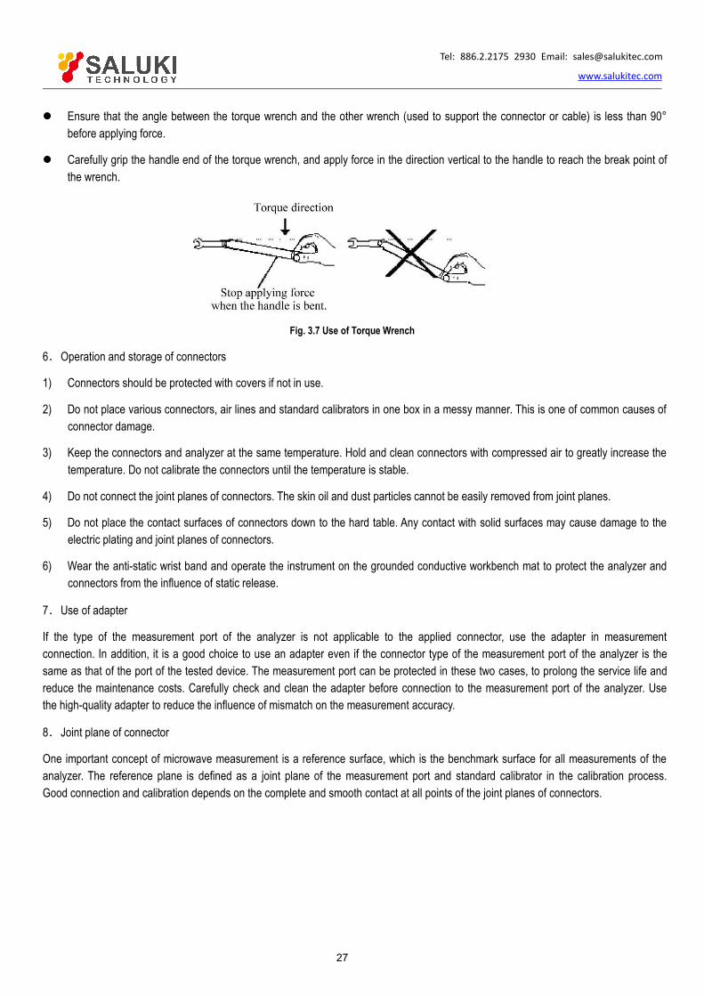
5.Use of torque wrench
The use of the torque wrench is shown in Fig. 3.7. Pay attention to the following items.
Check whether the torque of the torque wrench is set properly before use.
Tel: 886.2.2175 2930 Email: [email protected]
www.salukitec.com
27
Ensure that the angle between the torque wrench and the other wrench (used to support the connector or cable) is less than 90°before applying force.
Carefully grip the handle end of the torque wrench, and apply force in the direction vertical to the handle to reach the break point ofthe wrench.
Fig. 3.7 Use of Torque Wrench
6.Operation and storage of connectors
1) Connectors should be protected with covers if not in use.
2) Do not place various connectors, air lines and standard calibrators in one box in a messy manner. This is one of common causes ofconnector damage.
3) Keep the connectors and analyzer at the same temperature. Hold and clean connectors with compressed air to greatly increase thetemperature. Do not calibrate the connectors until the temperature is stable.
4) Do not connect the joint planes of connectors. The skin oil and dust particles cannot be easily removed from joint planes.
5) Do not place the contact surfaces of connectors down to the hard table. Any contact with solid surfaces may cause damage to theelectric plating and joint planes of connectors.
6) Wear the anti-static wrist band and operate the instrument on the grounded conductive workbench mat to protect the analyzer andconnectors from the influence of static release.
7.Use of adapter
If the type of the measurement port of the analyzer is not applicable to the applied connector, use the adapter in measurementconnection. In addition, it is a good choice to use an adapter even if the connector type of the measurement port of the analyzer is thesame as that of the port of the tested device. The measurement port can be protected in these two cases, to prolong the service life andreduce the maintenance costs. Carefully check and clean the adapter before connection to the measurement port of the analyzer. Usethe high-quality adapter to reduce the influence of mismatch on the measurement accuracy.
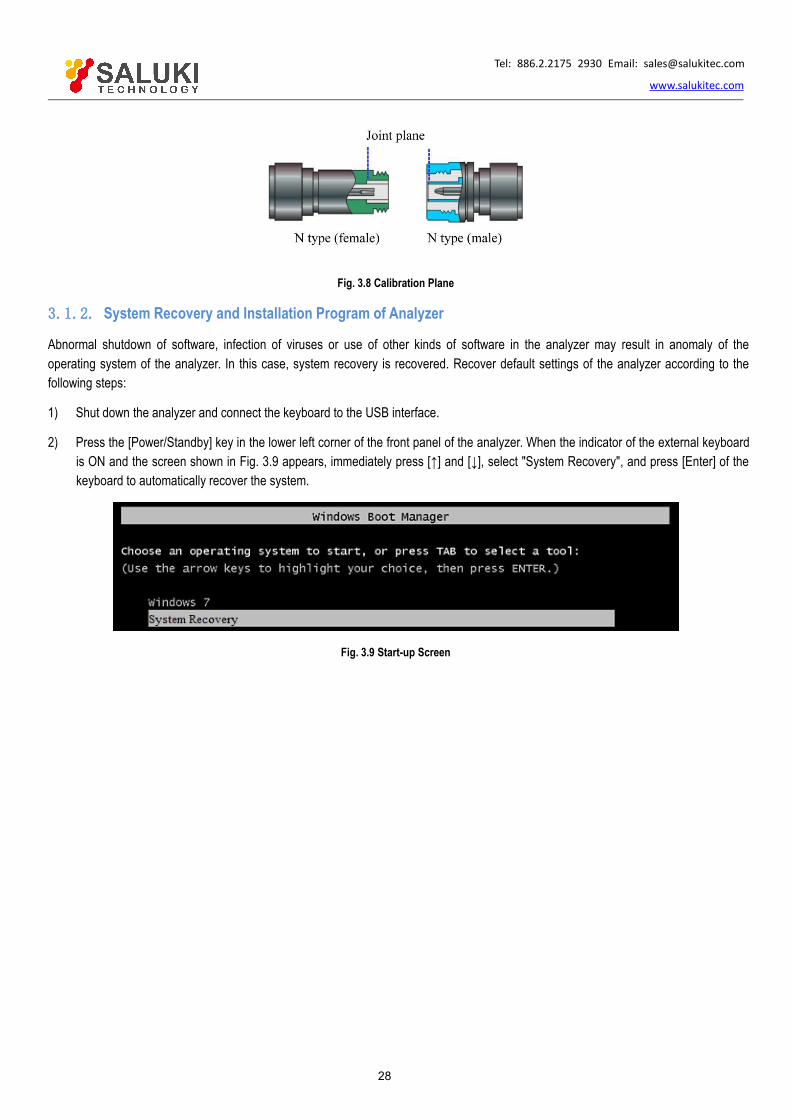
8.Joint plane of connector
One important concept of microwave measurement is a reference surface, which is the benchmark surface for all measurements of theanalyzer. The reference plane is defined as a joint plane of the measurement port and standard calibrator in the calibration process.Good connection and calibration depends on the complete and smooth contact at all points of the joint planes of connectors.
Tel: 886.2.2175 2930 Email: [email protected]
www.salukitec.com
28
Fig. 3.8 Calibration Plane
3.1.2. System Recovery and Installation Program of Analyzer
Abnormal shutdown of software, infection of viruses or use of other kinds of software in the analyzer may result in anomaly of theoperating system of the analyzer. In this case, system recovery is recovered. Recover default settings of the analyzer according to thefollowing steps:
1) Shut down the analyzer and connect the keyboard to the USB interface.
2) Press the [Power/Standby] key in the lower left corner of the front panel of the analyzer. When the indicator of the external keyboardis ON and the screen shown in Fig. 3.9 appears, immediately press [↑] and [↓], select "System Recovery", and press [Enter] of thekeyboard to automatically recover the system.
Fig. 3.9 Start-up Screen

Tel: 886.2.2175 2930 Email: [email protected]
www.salukitec.com
29
Fig. 3.10 System Recovery Screen
3) If the screen shown in Fig. 3.10 appears, system recovery is started. About 10min is required in the whole process of systemrecovery. Restart the analyzer after recovery.
3.1.3. Routine Maintenance
This section describes the routine maintenance of S3602 series vector network analyzers.
1) Cleaning of instrument surface
Clean the instrument surface according to the following steps:
Step 1: turn off the instrument by disconnecting the power line connected to the instrument.
Step 2: carefully wipe the surface with dry or slightly wet soft cloth. Do not wipe the inside of the instrument.
Step 3: do not use any chemical cleaner, such as alcohol, acetone or any cleaner which may be diluted.
2) Cleaning of display
Clean the display after a certain period of use. Follow the steps below:
Step 1: turn off the instrument by disconnecting the power line connected to the instrument.
Step 2: soak clean soft cloth with cleaner, and carefully wipe the display panel.
Step 3: dry the display with clean and soft cotton cloth.
Step 4: Connect the power line after the cleaner is thoroughly dry.

Tel: 886.2.2175 2930 Email: [email protected]
www.salukitec.com
30
Clean the display.
There is anti-static coating on display surface, do not use fluoride-bearing detergent or acidic/alkaline detergent. Do not spray detergenton display panel directly, otherwise it may penetrate into and damage the instrument
3.2.Front Panel & Rear PanelThis chapter introduces the elements and functions of the front panel, rear panel and operation interface of S3602 series vector networkanalyzer.
Front panel
Rear panel
3.2.1. Front Panel
This section introduces the structure and functions of the front panel of S3602 series vector network analyzer. The front panel is shown inthe following figure.
Fig. 3.11:Front Panel of S3602
1.Input Key zone
The keys are used to enter measurement Setups, as shown in Fig 3.12.
Fig. 3.12 Input Key Zone of S3602

Tel: 886.2.2175 2930 Email: [email protected]
www.salukitec.com
31
1) [OK] key
Confirm the Setups and input values in the dialog box and close the dialog box, equivalent to the "OK” button in the dialog box.
2) [Cancel] key
Ignore the Setups and input in the dialog box and close the dialog box, equivalent to the "Cancel” button in the dialog box.
3) [Soft Keyboard] key
Call the soft keyboard of the Windows 7 system.
4) [Backspace/←] key
Move the marker back and delete the original input after entering.
5) Number keys
Include 0-9. Enter the numbers in measurement Setup and press the corresponding unit keys to complete input.
6) Unit keys
End the number input and distribute a unit to each input value. The unit corresponding to each key is as follows:
[G/n] G/ns (109/10-9)[M/μ] M/μs (106/10-6)[k/m] k/ms (103/10-3)
Basic units include dB, dBm, degree, second, Hz or dB/GHz. The keys can also be used to input valueswith no unit and have the functions of the “Enter” key.
2.Adjustment key zone
Include navigation keys and knobs, as shown in Fig.3.13
Fig. 3.13 Adjustment Key Zone of S3602
1) Knob
Rotate the knob to adjust the set value in the current active input box.
2) [←] and [→] key
Move left or right to select the menu.
Switch the active options in the dialog box.
Tel: 886.2.2175 2930 Email: [email protected]
www.salukitec.com
32
3) [↑] and [↓] key
Move up and down in the menu to select the menu item. When interact with dialog box, the arrow keys can be used to change value,select item in the drop-down list, and select the desired option in a group of option list.
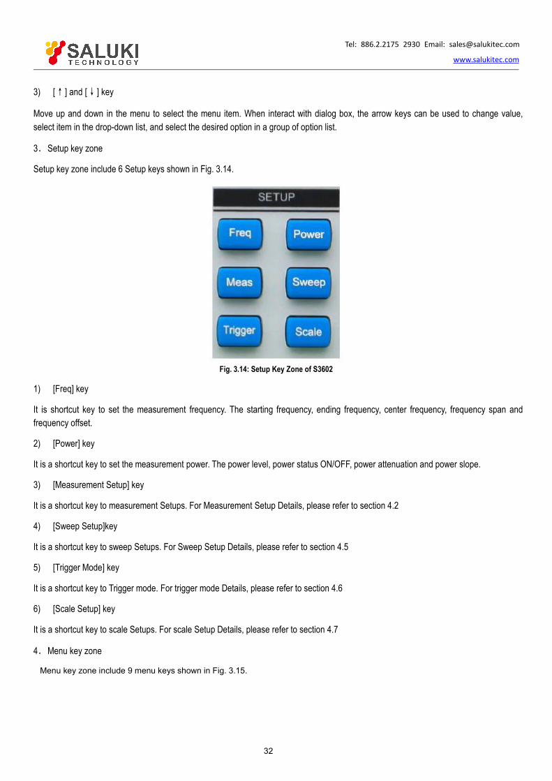
3.Setup key zone
Setup key zone include 6 Setup keys shown in Fig. 3.14.
Fig. 3.14: Setup Key Zone of S3602
1) [Freq] key
It is shortcut key to set the measurement frequency. The starting frequency, ending frequency, center frequency, frequency span andfrequency offset.
2) [Power] key
It is a shortcut key to set the measurement power. The power level, power status ON/OFF, power attenuation and power slope.
3) [Measurement Setup] key
It is a shortcut key to measurement Setups. For Measurement Setup Details, please refer to section 4.2
4) [Sweep Setup]key
It is a shortcut key to sweep Setups. For Sweep Setup Details, please refer to section 4.5
5) [Trigger Mode] key
It is a shortcut key to Trigger mode. For trigger mode Details, please refer to section 4.6
6) [Scale Setup] key
It is a shortcut key to scale Setups. For scale Setup Details, please refer to section 4.7
4.Menu key zone
Menu key zone include 9 menu keys shown in Fig. 3.15.

Tel: 886.2.2175 2930 Email: [email protected]
www.salukitec.com
33
Fig.3.15: Menu Key Zone of S3602
1) [File] key
Open the main file menu. Following options will be displayed on screen: “Save”, “Call”, “Print”, “Minimize application program” and “Exit”.
2) [Trace] key
Open the main Trace menu. Following options will be displayed on screen: “New Trace”, “Delete Trace”, “Select Trace”, “Move Trace”,“Trace title” and “Maximize Trace”.
3) [Channel] key
Open the main channel menu and the current channel will be selected automatically. Following options will be displayed on screen:“Channel 1/2/3/4”, “Open channel”, “Close channel”, “Select channel”, “Copy channel” and “Hardware Setup”.
4) [Stimulus] key
Open the main Stimulus menu. Following options will be displayed on screen: “Frequency”, “Power”, “Sweep” and “Trigger”.
5) [Response] key
Open the main response menu. Following options will be displayed on screen: “Measurement”, “Format”, “Scale”, “Display” and“Average”.
6) [Calibration] key
Open the main calibration menu. Following options will be displayed on screen: “Calibration”, “Correction ON/OFF”, “InterpolationON/OFF”, “Port extension”, “Fixture”, “Edit calibrator”, “Attribute” and “Power calibration”.
7) [marker] key
Open the main marker menu. Following options will be displayed on screen: “marker”, “marker function”, “marker search”, “markerattribute” and “marker display”. If no marker is enabled at present, the marker 1 will be enabled automatically in the default mode. If amarker is enabled, the current marker will be selected automatically.
8) [Analysis] key
Open the main analysis menu. Following options will be displayed on screen: “Save”, “Test”, “Trace statistics”, “Gate”, “Window”, “Timedomain”, “Structural return loss” and “Formula editor”.
9) [System] key
Open the main system menu. Following options will be displayed on screen: “Configuration”, “Record/Run”, “Spread spectrum”,“Windows task bar”, “Reset”, “Custom user reset state” and “Language”.

Tel: 886.2.2175 2930 Email: [email protected]
www.salukitec.com
34
5.Function Key Zone
Function key zone include 4 function keys on the left side of the screen as shown in Fig. 3.16.
Fig. 3.16: Function Key Zone of S3602
1) [Help] key
Open the main help menu. Following options will be displayed on screen: “User manual”, “Programming manual”, “Technical support”,“Error information” and “About”.
2) [Record/run] key
It is a shortcut key to enable the recording/running function of the analyzer. Press the key to automatically start recording. If recording iscompleted, press this key to automatically start running. This key is only effective for Record/Run 1, and cannot be used to controlRecord/Run 2.
3) [Macro/local] key
If the analyzer is programmed, press this key to switch to the macro state. If the analyzer is not programmed, press this key to open themacro menu.
4) [Preset]key
It is a shortcut key to reset the analyzer. If the user has saved the reset state and tick the item “Enable user reset state”, press this keyto recover the state saved by the user; otherwise, the system reset state will be recovered.
6.USB Interface
The USB interface can be connected with the keyboard, mouse and other USB devices. The front panel is equipped with four USBinterfaces in total and conforms to the USB2.0 specifications. The interface jack is of A type (four embedded contacts; Contact 1 on theleft side).
Fig. 3.17: USB Interface
7.Display screen

Tel: 886.2.2175 2930 Email: [email protected]
www.salukitec.com
35
The display screen of the analyzer is a TFT LCD screen. Technical indicators are as follows:
12.1-inch touch screen
Resolution: 1280×800
Vertical refresh rate: 60Hz
Horizontal refresh rate: 48.4Hz
8.[Start/Standby] key and indicator
The [Start/Standby] key and indicator are shown in Fig. 3.18. The power switch is used to start the analyzer or enable the standby stateof the analyzer.
The indicator is green when the analyzer is started.
The indicator is orange when the analyzer is in the standby state.
Press the power button to start the analyzer. Then the Windows 7 operating system will be run automatically and the measurementapplication program will be loaded.
When the power button is pressed in the standby state, the analyzer will automatically exit the application program. When thepower supply will be turned off, the standby state will be enabled.
This is only a standby switch. It cannot be directly connected with the external power supply or used to cut off the connectionbetween the instrument and external power supply. The external power supply of the analyzer can be shut down by the powerswitch on the rear panel. The connection between the analyzer and external power supply can be fully cut off by removing thepower cable.
Fig. 3.18: [Start/Standby] Key and Indicator
9.Test port
As shown in Fig. 3.19, the instrument is equipped with 2x 50Ω ports and 2x 3.5mm/2.4mm/1.85mm ports (male). The instrument can actas both RF source and receiver. so as to measure the tested device in bi-directions. The yellow light indicates the source output port.
Fig. 3.19: Test Ports of Analyzer
3.2.2. Rear Panel
This section introduces the structure and functions of the rear panel of S3602 series vector network analyzer. The rear panel is shown inthe following figure.
Tel: 886.2.2175 2930 Email: [email protected]
www.salukitec.com
36
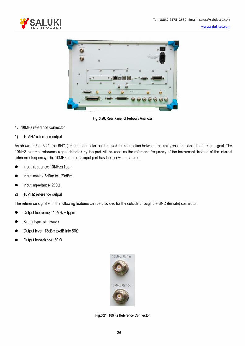
Fig. 3.20: Rear Panel of Network Analyzer
1.10MHz reference connector
1) 10MHZ reference output
As shown in Fig. 3.21, the BNC (female) connector can be used for connection between the analyzer and external reference signal. The10MHZ external reference signal detected by the port will be used as the reference frequency of the instrument, instead of the internalreference frequency. The 10MHz reference input port has the following features:
Input frequency: 10MHz±1ppm
Input level: -15dBm to +20dBm
Input impedance: 200Ω
2) 10MHZ reference output
The reference signal with the following features can be provided for the outside through the BNC (female) connector.
Output frequency: 10MHz±1ppm
Signal type: sine wave
Output level: 13dBm±4dB into 50Ω
Output impedance: 50 Ω
Fig.3.21: 10MHz Reference Connector

Tel: 886.2.2175 2930 Email: [email protected]
www.salukitec.com
37
2.General-interface bus connector
As shown in Fig.3.22 this is a 24-pin D-type female connector, meeting the IEEE-488 standards. It is used to transmit and receiveGPIB/SCPI commands.
Fig. 3.22: General-interface Bus Connector
3.LAN connector
As shown in Fig. 3.23, this is a 10/100/1000BaseT Ethernet connector of standard 8-pin structure, and three data rates can be selected.
Fig. 3.23: LAN Connector
4.USB connector
As shown in Fig. 3.24, the connector jack is of Type A (four embedded contacts; with Contact 1 on the left side) and Type B. Type Aconnector can be connected to the USB mouse, keyboard or other USB interface devices. The rear panel is equipped with four interfacesin total.
Type B connector is mainly used for control. The network analyzer can be connected to the external computer or remote device throughSCPI control. The rear panel is equipped with one interface.
Fig. 3.24: USB Connector (B-type on the left and A-type on the right)
5.Video graphic adapter (VGA) output connector
As shown in Fig. 3.25, this is a 15-pin D-sub female connector to be connected with the external VGA display of corresponding resolution.In this case, the user can observe the internal and external display at the same time.

Tel: 886.2.2175 2930 Email: [email protected]
www.salukitec.com
38
Fig. 3.25: VGA Connector
6.LO and RF output connector
As shown in Fig. 3.26, the 3.5mm female interface is used for LO output and RF output. The LO interface is used for internal LO signaloutput, and RF interface for RF source signal output. The connector can be used for fault detection and millimeter wave spreading. Theinterface features are as follows:
Frequency range of LO output signal:
12.535MHz-13.507606GHz/26.507606GHz/43.507606GHz/50.007606GHz/67.007606GHz
Power range of LO output signal: -4dBm to 6dBm
Frequency range of RF output signal: 3.2GHz-13.5GHz/26.5GHz/43.5GHz/50GHz/67GHz
RF output signal power: -3dBm±2dB
Fig. 3.26: LO and RF Output Connector
7.Pulse input/output connector
As shown in Fig. 3.27, this is a 15-pin D-type female connector. The working status of the internal pulse generator can be monitoredsynchronously through this interface.
Fig. 3.27: Pulse Input/Output Connector
8.External IF input connector
As shown in Fig. 3.28, five SMA interfaces are used for external IF input of the vector network. The two-port model is marked with A, B,R1 and R2, and the four-port with A, B, C, D and R.
Fig. 3.28: Intermediate Input Connector

Tel: 886.2.2175 2930 Email: [email protected]
www.salukitec.com
39
9.Automatic test interface connector
As shown in Fig. 3.29, this interface is a 36-pin female connector. The network analyzer and material handler can exchange signalsthrough this interface to provide a stable and reliable automatic test environment for the user.
Fig. 3.29: Automatic Test Interface Connector
10.Extension interface connector
As shown in Fig. 3.30, this interface is a 9-pin D-type female connector.
Fig. 3.30: Extension Interface Connector
11.External tester interface connector
As shown in Fig. 3.31, this tester interface is a DB-25 female interface, including 13 addresses and data multiplexing lines, three controllines and one interruption control line, and is used to control the external tester (such as the external spread spectrum controller).
Fig. 3.31: External Tester Interface Connector
12.Trigger input/output interface connector
As shown in Fig. 3.32, this interface is an external and auxiliary trigger input/output interface. Specific functions are as follows:
External trigger input - if it is enabled, the vector network analyzer will be triggered according to the connected signal.
External trigger ready - if it is enabled, the vector network analyzer will send a “Ready” signal to the external device through thisinterface.
Auxiliary trigger input 1/2 - if it is enabled, the external device will send an “OK” signal (meaning the external device is ready toreceive trigger signal) to the vector network analyzer through this interface.
Auxiliary trigger output 1/2 - if it is enabled, the vector network analyzer will send an “OK” signal through this interface before (or
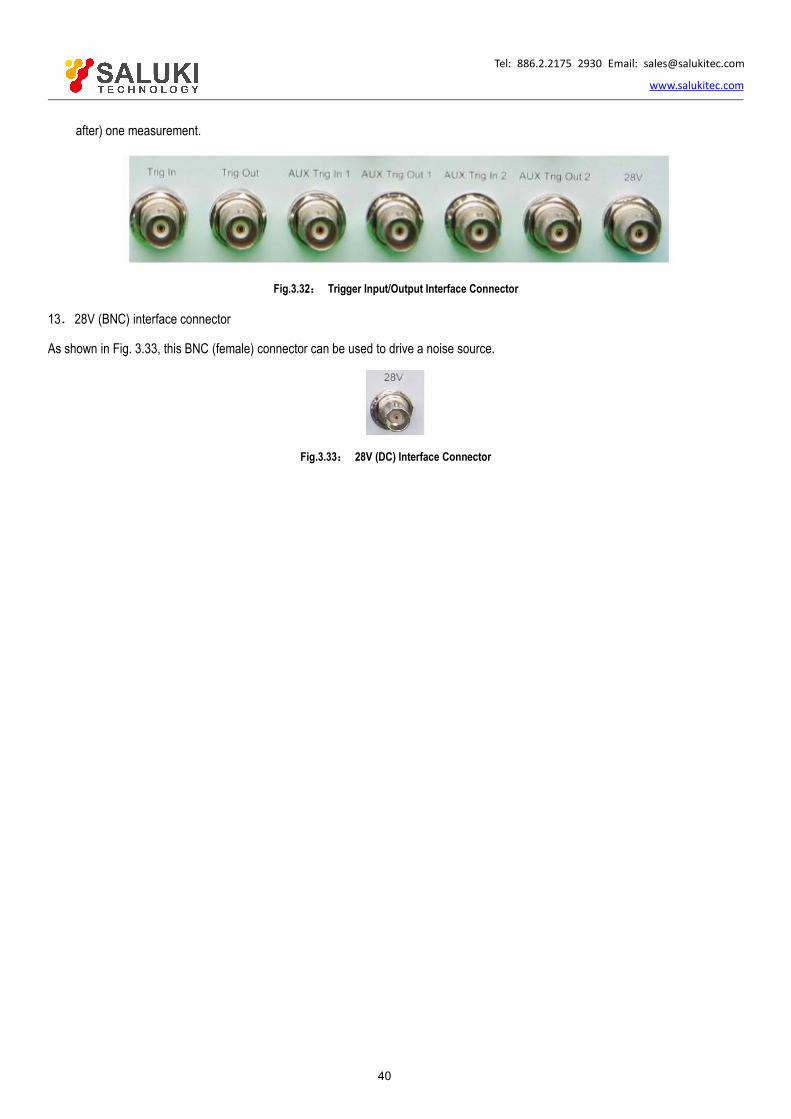
Tel: 886.2.2175 2930 Email: [email protected]
www.salukitec.com
40
after) one measurement.
Fig.3.32: Trigger Input/Output Interface Connector
13.28V (BNC) interface connector
As shown in Fig. 3.33, this BNC (female) connector can be used to drive a noise source.
Fig.3.33: 28V (DC) Interface Connector
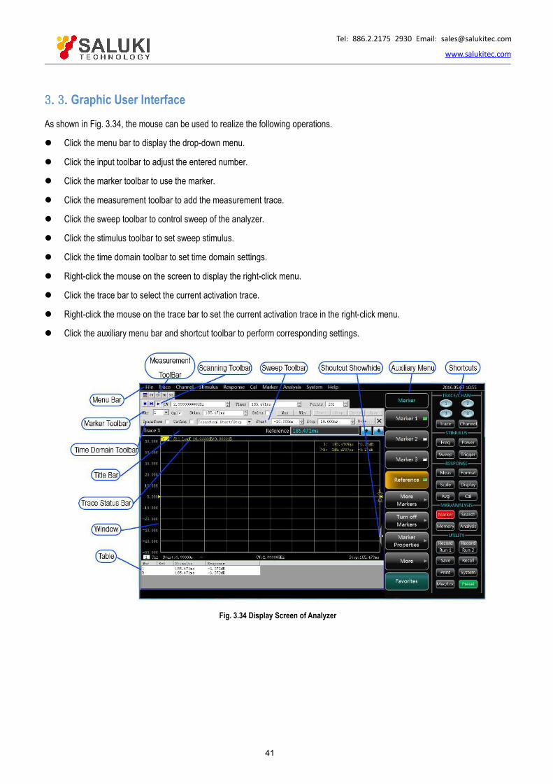
Tel: 886.2.2175 2930 Email: [email protected]
www.salukitec.com
41
3.3.Graphic User Interface
As shown in Fig. 3.34, the mouse can be used to realize the following operations.
Click the menu bar to display the drop-down menu.
Click the input toolbar to adjust the entered number.
Click the marker toolbar to use the marker.
Click the measurement toolbar to add the measurement trace.
Click the sweep toolbar to control sweep of the analyzer.
Click the stimulus toolbar to set sweep stimulus.
Click the time domain toolbar to set time domain settings.
Right-click the mouse on the screen to display the right-click menu.
Click the trace bar to select the current activation trace.
Right-click the mouse on the trace bar to set the current activation trace in the right-click menu.
Click the auxiliary menu bar and shortcut toolbar to perform corresponding settings.
Fig. 3.34 Display Screen of Analyzer

Tel: 886.2.2175 2930 Email: [email protected]
www.salukitec.com
42
3.4.Trace, Channel and Window of Analyzer
Trace
Channel
Window
3.4.1. TraceThe trace is a series of measurement data points. Trace settings will affect the mathematical operation and display of measurementdata. Only the settings of the active trace can be changed. Click the corresponding trace status button to active the trace. Fordetailed setting, refer to "change trace activation status" of "4.2 Selection of Measurement Parameter". Trace settings include:
Measured parameters
Display format
Scale
Trace operation
Marker
Electrical delay
phase offset
Smoothing
Time domain transformation
3.4.2. Channel
The channel is a trace container. The analyzer supports 64 channels in total. Channel settings are associated with measurement ofthe trace in the channel. The same channel settings are applicable to tracks in the same channel. Only the settings of the activechannel can be changed. Once the trace in the channel is activated, the channel will also be activated. For detailed settings of theactive trace, refer to "change trace activation status" of "4.2 Selection of Measurement Parameter".Channel settings include:
Frequency span
Power
Standard data
Intermediate-frequency bandwidth
Number of sweep points
Sweep setting
Average
Trigger (for some settings)
3.4.3. WindowThe window is used to observe the measurement trace. The analyzer supports 32 windows at most, and eight tracks can bedisplayed at most in each window. Set the window display by the [View] menu. For details, refer to "4.9 Setting of Analyzer Display".
1.Create a new window.
Menu path: [Response] > [Display] > [Window] > [New window]. Then a new window will be created. The default setting of the tracein the window is S11, indicating Channel 1.
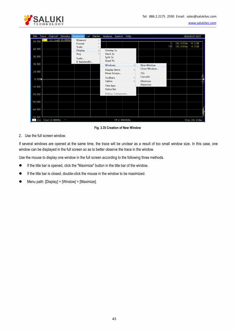
Tel: 886.2.2175 2930 Email: [email protected]
www.salukitec.com
43
Fig. 3.35 Creation of New Window
2.Use the full screen window.
If several windows are opened at the same time, the trace will be unclear as a result of too small window size. In this case, onewindow can be displayed in the full screen so as to better observe the trace in the window.
Use the mouse to display one window in the full screen according to the following three methods.
If the title bar is opened, click the "Maximize" button in the title bar of the window.
If the title bar is closed, double-click the mouse in the window to be maximized.
Menu path: [Display] > [Window] > [Maximize].
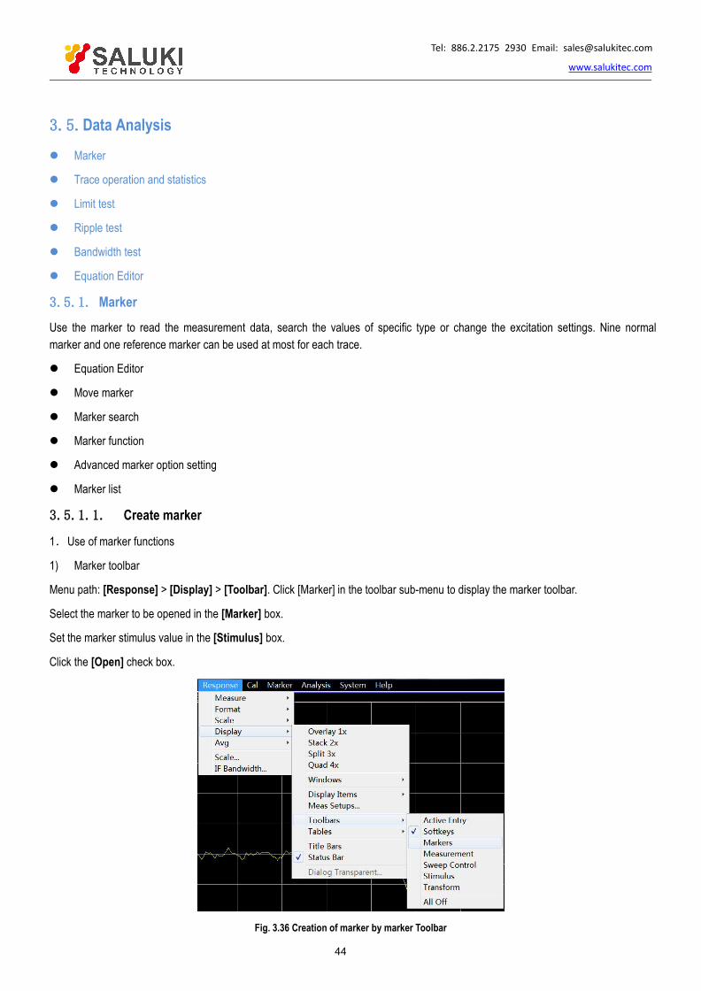
Tel: 886.2.2175 2930 Email: [email protected]
www.salukitec.com
44
3.5.Data Analysis
Marker
Trace operation and statistics
Limit test
Ripple test
Bandwidth test
Equation Editor
3.5.1. MarkerUse the marker to read the measurement data, search the values of specific type or change the excitation settings. Nine normalmarker and one reference marker can be used at most for each trace.
Equation Editor
Move marker
Marker search
Marker function
Advanced marker option setting
Marker list
3.5.1.1. Create marker
1.Use of marker functions
1) Marker toolbar
Menu path: [Response] > [Display] > [Toolbar]. Click [Marker] in the toolbar sub-menu to display the marker toolbar.
Select the marker to be opened in the [Marker] box.
Set the marker stimulus value in the [Stimulus] box.
Click the [Open] check box.
Fig. 3.36 Creation of marker by marker Toolbar
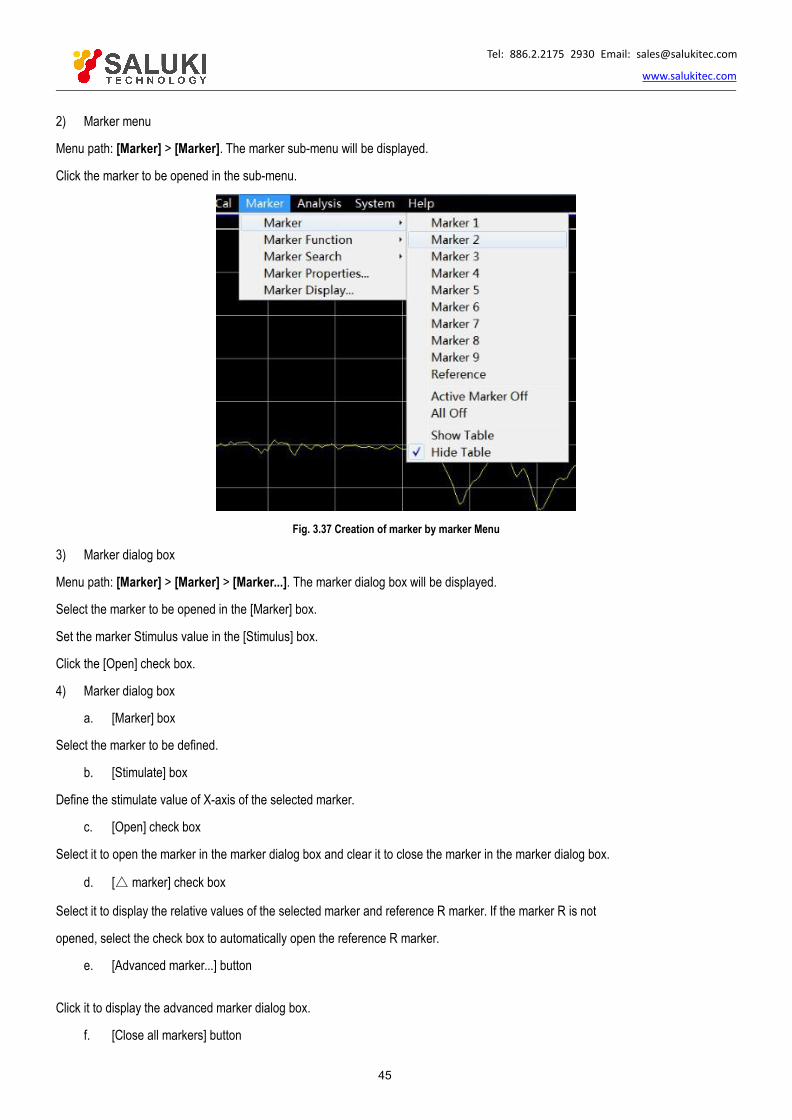
Tel: 886.2.2175 2930 Email: [email protected]
www.salukitec.com
45
2) Marker menu
Menu path: [Marker] > [Marker]. The marker sub-menu will be displayed.
Click the marker to be opened in the sub-menu.
Fig. 3.37 Creation of marker by marker Menu
3) Marker dialog box
Menu path: [Marker] > [Marker] > [Marker...]. The marker dialog box will be displayed.
Select the marker to be opened in the [Marker] box.
Set the marker Stimulus value in the [Stimulus] box.
Click the [Open] check box.
4) Marker dialog box
a. [Marker] box
Select the marker to be defined.
b. [Stimulate] box
Define the stimulate value of X-axis of the selected marker.
c. [Open] check box
Select it to open the marker in the marker dialog box and clear it to close the marker in the marker dialog box.
d. [ marker] check box
Select it to display the relative values of the selected marker and reference R marker. If the marker R is not
opened, select the check box to automatically open the reference R marker.
e. [Advanced marker...] button
Click it to display the advanced marker dialog box.
f. [Close all markers] button

Tel: 886.2.2175 2930 Email: [email protected]
www.salukitec.com
46
Click it to close all the opened marker.
3.5.1.2. Move marker1) Activate the marker to be moved in one of the above three methods.
2) Move the marker in one of the following methods.
a. Click the [Stimulate] box in the marker dialog box and move the marker in the following method.
Directly enter the marker stimulate value.
Rotate the knob to move the marker.
Click the [↑] or [↓] in the [Stimulate] box to change the marker stimulate value.
Press [↑] or [↓] in the adjustment key zone to change the marker stimulate value.
b. Click the [Stimulate] box in the marker toolbar and move the marker in the following method.
Directly enter the stimulus value.
Rotate the knob to move the marker.
Click the [↑] or [↓] in the [Stimulate] box to change the marker stimulate value.
Press [↑] or [↓] in the adjustment key zone to change the marker stimulate value.
c. Move the marker in the input toolbar in the following method.
Directly enter the stimulate value.
Rotate the knob to change the stimulate value.
Press [↑] or [↓] in the adjustment key zone to change the marker stimulate value.
click the Up and Down arrow in the input box to change the marker stimulate value.
3.5.1.3. Marker searchSearch the specific measured value with the marker searching function. If no matching measurement data are found, the marker willremain unchanged in the current position.
1) Marker search method:
Menu path: [Marker] > [Marker search].
Set the marker search in the dialog box. Click [Execute] to execute marker search and [OK] to close the dialog box.
Fig. 3.38 Marker Search
2) Marker search dialog box
a. Marker zone
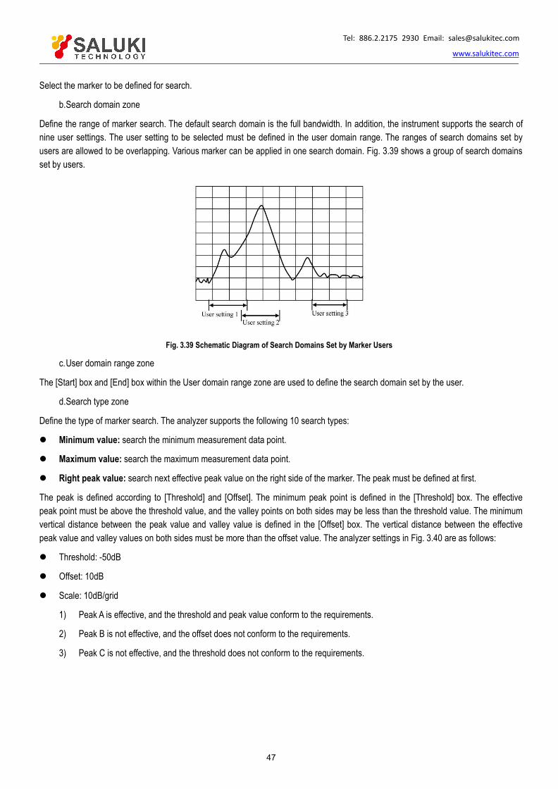
Tel: 886.2.2175 2930 Email: [email protected]
www.salukitec.com
47
Select the marker to be defined for search.
b.Search domain zone
Define the range of marker search. The default search domain is the full bandwidth. In addition, the instrument supports the search ofnine user settings. The user setting to be selected must be defined in the user domain range. The ranges of search domains set byusers are allowed to be overlapping. Various marker can be applied in one search domain. Fig. 3.39 shows a group of search domainsset by users.
Fig. 3.39 Schematic Diagram of Search Domains Set by Marker Users
c.User domain range zone
The [Start] box and [End] box within the User domain range zone are used to define the search domain set by the user.
d.Search type zone
Define the type of marker search. The analyzer supports the following 10 search types:
Minimum value: search the minimum measurement data point.
Maximum value: search the maximum measurement data point.
Right peak value: search next effective peak value on the right side of the marker. The peak must be defined at first.
The peak is defined according to [Threshold] and [Offset]. The minimum peak point is defined in the [Threshold] box. The effectivepeak point must be above the threshold value, and the valley points on both sides may be less than the threshold value. The minimumvertical distance between the peak value and valley value is defined in the [Offset] box. The vertical distance between the effectivepeak value and valley values on both sides must be more than the offset value. The analyzer settings in Fig. 3.40 are as follows:
Threshold: -50dB
Offset: 10dB
Scale: 10dB/grid
1) Peak A is effective, and the threshold and peak value conform to the requirements.
2) Peak B is not effective, and the offset does not conform to the requirements.
3) Peak C is not effective, and the threshold does not conform to the requirements.

Tel: 886.2.2175 2930 Email: [email protected]
www.salukitec.com
48
Fig. 3.40 Schematic Diagram of Peak in marker Domain
Left peak: search next effective peak value on the left side of the marker. The peak must be defined at first.
Next peak: search next peak lower than the current marker amplitude. The peak must be defined at first.
Target: enter the search target value in the [Log] box and click [Execute]. The marker will move to the first target value on theright side of the current marker location. Then continuously click [Execute], and the marker will move to next target value on theright side until it reaches the maximum stimulus value. In this case, the marker will return to the lowest stimulus value to searchthe target value.
If the [Discrete marker] is selected in the [Advanced marker] dialog box, the marker will move to the discrete data pointcorresponding to the target value.
If the [Discrete marker] is cleared in the [Advanced marker] dialog box, the marker will move to the interpolation data pointcorresponding to the target value.
Left target: only search the target value on the left side of the current marker.
Right target: only search the target value on the right side of the current marker.
Bandwidth: if the bandwidth searching function is selected, set the level (default: -3dB) below the peak in the level box andmeasure the bandwidth at the set level, as shown in Fig. 3.41. Use marker 1-4 for measurement. marker 1 is used to search themaximum peak value, marker 2 to search the point of specified level on the left side of the peak, marker 3 to search the point ofspecified level on the right side of the peak, and marker 4 to search the center of the bandwidth. The following information will bedisplayed after measurement.
Bandwidth: frequency difference between the right and left cutoff frequency point.
Center: frequency of the middle point between the right and left cutoff frequency point.
Q: value calculated by dividing the center frequency by the bandwidth.
Loss: value measured at the center frequency point of the bandwidth.
Left cutoff: minimum frequency of two points below the specific bandwidth level of the signal peak.
Right cutoff: maximum frequency of two points below the specific bandwidth level of the signal peak.

Tel: 886.2.2175 2930 Email: [email protected]
www.salukitec.com
49
Fig. 3.41 Bandwidth Search
Filter test: the analyzer has a special shortcut function to test the filter, and all test parameters will be automatically displayed onthe screen so that the user can directly observe measurement results. As manual setting in the test is eliminated, the speed offilter test is greatly increased. As shown in Fig. 3.42.
Eight parameters of the filter test are displayed in the upper left corner of the trace. When the filter test is started, bandwidth searchwill be automatically enabled, and six parameters of the bandwidth test will be displayed in the upper right corner at the same time.
Level of Bandwidth 1: set the level of Bandwidth 1 in the input box.
Level of Bandwidth 2: set the level of Bandwidth 2 in the input box.
Percentage frequency offset: set the percentage of frequency offset in the input box.
Fig. 3.42 Filter Test
a) [Execute] button
Click the [Execute] button to execute one marker search of specified type.
b) [Tracking] check box
If [Tracking] is selected, the search function will be executed after each sweep according to the current search type and domainsetting. In this case, the marker will be in the desired position after each sweep.
3.5.1.4. Marker function
1.Use of marker functions
Some settings of the instrument can be changed according to the marker activation position, such as the starting frequency, endingfrequency, etc. The setting method is as follows.
Menu path: [Marker] > [Marker function].
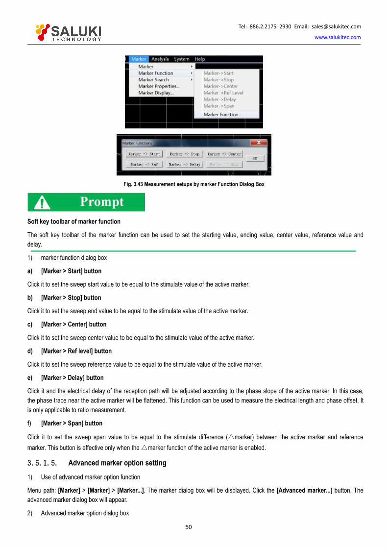
Tel: 886.2.2175 2930 Email: [email protected]
www.salukitec.com
50
Fig. 3.43 Measurement setups by marker Function Dialog Box
Soft key toolbar of marker function
The soft key toolbar of the marker function can be used to set the starting value, ending value, center value, reference value anddelay.
1) marker function dialog box
a) [Marker > Start] button
Click it to set the sweep start value to be equal to the stimulate value of the active marker.
b) [Marker > Stop] button
Click it to set the sweep end value to be equal to the stimulate value of the active marker.
c) [Marker > Center] button
Click it to set the sweep center value to be equal to the stimulate value of the active marker.
d) [Marker > Ref level] button
Click it to set the sweep reference value to be equal to the stimulate value of the active marker.
e) [Marker > Delay] button
Click it and the electrical delay of the reception path will be adjusted according to the phase slope of the active marker. In this case,the phase trace near the active marker will be flattened. This function can be used to measure the electrical length and phase offset. Itis only applicable to ratio measurement.
f) [Marker > Span] button
Click it to set the sweep span value to be equal to the stimulate difference (marker) between the active marker and referencemarker. This button is effective only when themarker function of the active marker is enabled.
3.5.1.5. Advanced marker option setting
1) Use of advanced marker option function
Menu path: [Marker] > [Marker] > [Marker...]. The marker dialog box will be displayed. Click the [Advanced marker...] button. Theadvanced marker dialog box will appear.
2) Advanced marker option dialog box

Tel: 886.2.2175 2930 Email: [email protected]
www.salukitec.com
51
a) [Marker] box
Select the marker to be set.
b) [Open] check box
If this check box is selected, the corresponding marker will be displayed on the screen. If this check box is cleared, the marker displaywill be shut down.
c) [Discrete] check box
If this check box is selected, the data of the actual measurement point will be displayed. If this check box is cleared, the interpolationdata point between measurement points is still displayed.
d) [Format] box
Select the marker data format. The marker data format may be different from the format of trace data on the screen. The aboveformats are identical in the default mode.
e) Marker type zone
[Normal] option box
The X-axis location of the standard marker is fixed, while the Y-axis location changes with the trace data amplitude. The marker canbe moved right and left on the X-axis by changing the stimulus value.
[Fixed] option box
The X-axis and Y-axis coordinates of the marker set to be of fixed type remain fixed on the trace and do not change with the trace dataamplitude. The marker can be moved on the X-axis by changing the stimulus value, however, the Y-axis coordinate remainsunchanged. This kind of marker is mainly used to observe changes of trace data. For example, the fix marker can be used to compareinsertion loss changes before and after filter tuning.
3.5.1.6. Marker list1) Marker list
All marker data of the active data can be displayed by opening the marker list, in the format specified for the corresponding data. Themarker list will be opened and closed in the following method.
2) Open/Close method
Menu path 1: [Marker] > [Marker] > [Show Table] to open the marker list or [Hide Table] to close the marker list.
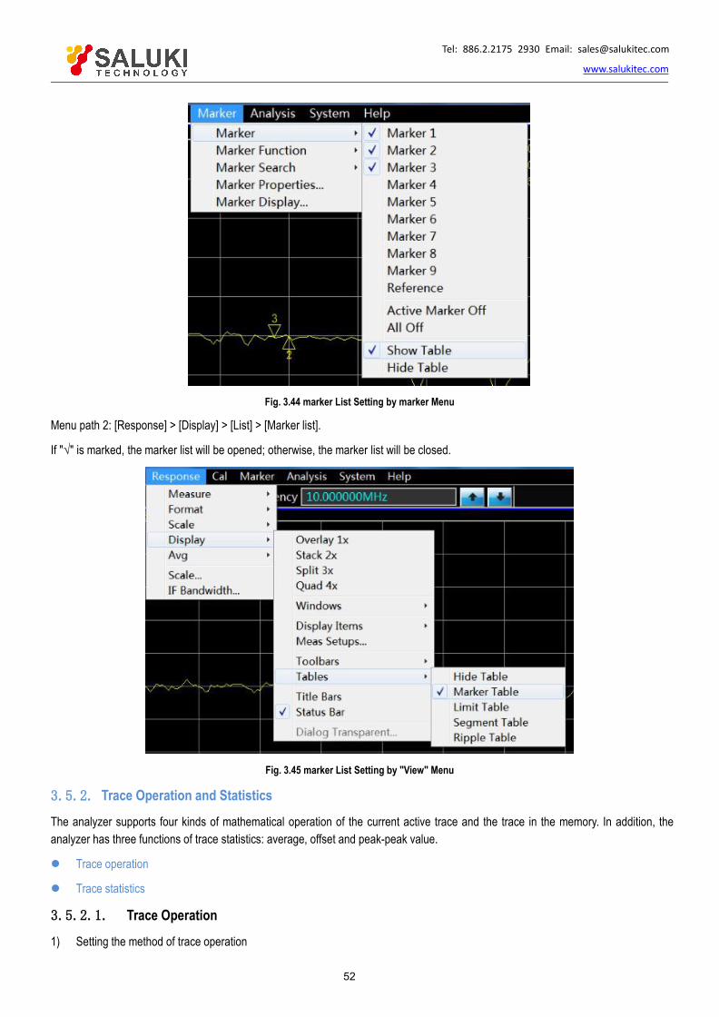
Tel: 886.2.2175 2930 Email: [email protected]
www.salukitec.com
52
Fig. 3.44 marker List Setting by marker Menu
Menu path 2: [Response] > [Display] > [List] > [Marker list].
If "√" is marked, the marker list will be opened; otherwise, the marker list will be closed.
Fig. 3.45 marker List Setting by "View" Menu
3.5.2. Trace Operation and Statistics
The analyzer supports four kinds of mathematical operation of the current active trace and the trace in the memory. In addition, theanalyzer has three functions of trace statistics: average, offset and peak-peak value.
Trace operation
Trace statistics
3.5.2.1. Trace Operation
1) Setting the method of trace operation

Tel: 886.2.2175 2930 Email: [email protected]
www.salukitec.com
53
One trace must be stored in the memory before setting the method of trace operation or performing any kind of trace operation. traceoperation is a kind of vector operation based on plural data before display formatting. It is set in the following method.
Menu path: [Analysis] > [Memory] > [Math/Memory...]. Then the operation/storage dialog box will appear.
Fig. 3.46 Setting of Trace Operation
2) Math/Memory dialog box
a) [Data > Memory] button
Save the current measurement data into the memory.
b) [Trace View Options] box
The [Trace View Options] box is used to select the type of trace operation. The analyzer supports the following operations.
Data
No mathematical operation.
Data+storage
The displayed trace data are the measured data plus stored trace data.
Data-storage
The displayed trace data are the measured data minus stored trace data. This function can be used for simple correction of errors. Atfirst, store the measured vector error into the memory, and then reduce the measurement data of the tested device by the measurederror.
. Data * storage
The displayed trace data are the measured data multiplied by the stored trace data.
Data/storage
The displayed trace data are the measured data divided by the stored trace data. This function is mainly used to measure the ratio,such as the gain and attenuation.
c) Data display selection zone
[Data trace] option box
Only display the data trace.
[Memory trace] option box

Tel: 886.2.2175 2930 Email: [email protected]
www.salukitec.com
54
Only display the memory trace.
[Data and memory] option box
Display the data trace and memory trace at the same time.
3.5.2.2. Trace Statistics
The analyzer has three functions of trace statistics: mean, offset and peak-peak value. The statistical values can be calculated withinthe whole stimulus bandwidth or user-defined bandwidth. Each channel supports nine user setting ranges, which are the same as thesearch domains set by user in the function of marker search. The same memory address is applied, so the same stimulus settings areshared. If the search domain to be set by the channel user is defined by marker search, the same stimulus settings can be called byselecting the corresponding user settings in trace statistics. The ranges of user settings are allowed to be overlapping.
It is not required to search the maximum and minimum value in the function of trace statistics, and the peak-peak value of pass bandripple can be measured easily. The statistical values of trace are calculated according to the data display format.
Rectangular coordinate format: the statistical values of trace are calculated according to the displayed scalar data.
Polar coordinate and Smith chart format: the statistical values of trace are calculated according to the value displayed in the logmagnitude format.
3) Activation of trace statistics
Menu path: [Analysis] > [Trace statistics]. The dialog box of trace statistics will appear.
Fig. 3.47 Dialog Box of trace Statistics
4) Dialog box of Trace statistics
a) [Statistics > Peak to Peak, Mean, Standard Deviation, Max, Min] check box
If this check box is selected, the function of trace statistics will be enabled. If this check box is cleared, the function of trace statisticswill be disabled.
b) [Span] box
Set the span of trace statistics. Nine user settings can be selected within the whole bandwidth or customized, or the user settings canbe customized through the marker search dialog box.
c) User domain definition zone
[Start] box
Customize the starting value of the user setting span.
[Stop] box
Customize the ending value of the user setting span.
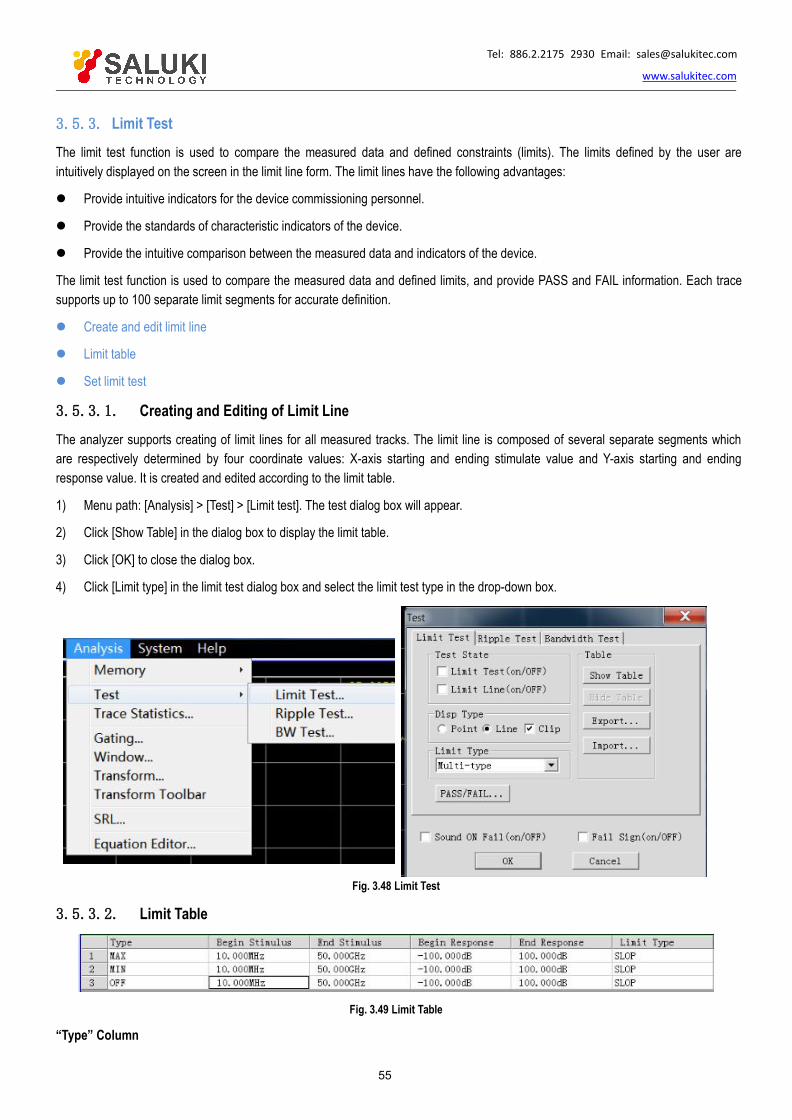
Tel: 886.2.2175 2930 Email: [email protected]
www.salukitec.com
55
3.5.3. Limit TestThe limit test function is used to compare the measured data and defined constraints (limits). The limits defined by the user areintuitively displayed on the screen in the limit line form. The limit lines have the following advantages:
Provide intuitive indicators for the device commissioning personnel.
Provide the standards of characteristic indicators of the device.
Provide the intuitive comparison between the measured data and indicators of the device.
The limit test function is used to compare the measured data and defined limits, and provide PASS and FAIL information. Each tracesupports up to 100 separate limit segments for accurate definition.
Create and edit limit line
Limit table
Set limit test
3.5.3.1. Creating and Editing of Limit LineThe analyzer supports creating of limit lines for all measured tracks. The limit line is composed of several separate segments whichare respectively determined by four coordinate values: X-axis starting and ending stimulate value and Y-axis starting and endingresponse value. It is created and edited according to the limit table.
1) Menu path: [Analysis] > [Test] > [Limit test]. The test dialog box will appear.
2) Click [Show Table] in the dialog box to display the limit table.
3) Click [OK] to close the dialog box.
4) Click [Limit type] in the limit test dialog box and select the limit test type in the drop-down box.
Fig. 3.48 Limit Test
3.5.3.2. Limit Table
Fig. 3.49 Limit Table
“Type” Column

Tel: 886.2.2175 2930 Email: [email protected]
www.salukitec.com
56
The Type box is used to set the limit test type:
MAX: the limit test fails if the trace is above the limit segment.
MIN: the limit test fails if the trace is below the limit segment.
OFF: disable the test of the limit segment.
“Begin Stimulus” / “End Stimulus” Column
Set the starting and ending stimulus value of the limit segment (i.e. X-axis starting and ending coordinate of the limit segment).
“Begin Response” Column and “Ending response” Column
Set the starting and ending response value of the limit segment (i.e. Y-axis starting and ending coordinate of the limit segment).
“Limit type” Column
Set the limit line display mode of the limit test:
SLOP: display the slope limit line.
FLAT: display the flat limit line.
POINT: display the point limit line.
3.5.3.3. Setting of Limit Test
After creating the limit line, select the mode of displaying or hiding the limit line of one trace. Even if the limit line is hided, thecorresponding limit test is still effective. The limit test is not applicable to the stored trace. You can select to send the warning soundand display the failure sign (FAIL) in case of the failure of limit test. When the limit test function is enabled, the trace of the failure partis red in the default mode. You can change the limit failure color in the Color setting" of the right-click menu of the mouse, and thetrace color of the passing part remains unchanged.
1) Setting method
a) Menu path: [Analysis] > [Test] - [Limit test]. The test dialog box will appear.
b) Set the limit test in the dialog box.
c) Click [OK] to close the dialog box.
The limit test can only be done at the actual sweep measurement point. The instrument can still pass the limit test if only a few sweeppoints are applied and the performance indicators of the tested device may not conform to the requirements. Therefore, sufficientsweep points should be applied in actual measurement of the limit test.
2) Limit test dialog box
[Limit test ON/OFF] check box
If this check box is selected, the limit test of the active trace will be enabled. If this check box is cleared, the limit test of the activetrace will be disabled.
[Limit line display ON/OFF] check box
If this check box is selected, the limit line of the active trace will be displayed on the screen. If this check box is cleared, the limit linedisplay of the active trace will be turned off, however, the limit test function will not be affected.
[SOUND on Fail (ON/OFF)] check box
If this check box is selected, the buzzer will send the warning sound in case of failure of the trace data point test.
[FAIL Sign (ON/OFF)] check box
If this check box is selected, the FAIL sign will be displayed on the screen in case of failure of the trace data point test.

Tel: 886.2.2175 2930 Email: [email protected]
www.salukitec.com
57
[Point] option box
If this box is selected, the discrete limit value corresponding to the measurement data point will be indicated with the symbol "v"(measurement type: MAX) and "^" (measurement type: MIN).
[Line] option box
If this box is selected, all the discrete limit setting points will be connected through a line.
[Show table] button
Click it to display and edit the limit table. If the limit table is opened, this button will be disabled.
[Hide table] button
Click it to close the limit table display. If the limit table is closed, this button will be disabled.
[Export] button
Click it and the storage dialog box will pop up. You can select the storage path, and the file will be saved in the “*.csv” format.
[Import] button
Click it and the storage dialog box will pop up. Select the storage path of the file to be opened, and the file will be opened in the *.csv"format.
[Limit type] drop-down option box
Click this drop-down option box to select the limit test type. Four types are provided in total: multi-type limit line, slope limit line,single-point limit line and flat limit line.
3.5.4. Ripple Test
The conformity of test results can be evaluated by setting the ripple limit of the ripple test. The measured data and defined ripple limitare compared in the test. The PASS and FAIL information will be provided, and the measurement results will be intuitively displayedon the screen. Each trace supports 12 separate limit segments at most. You can set the starting stimulus, ending stimulus andmaximum fluctuation of each limit segment. The stimulus settings of different segments may be overlapping.
3.5.4.1. Creating and Editing of Ripple Limit LineThe ripple limit test can be done to several tracks at the same time. The ripple limit can be set after the trace is activated.
1) Setting method
a) Menu path: [Analysis] > [Test] > [Ripple test]. The test dialog box will appear.
b) Click the [Show table] button in the dialog box to open the ripple limit table.
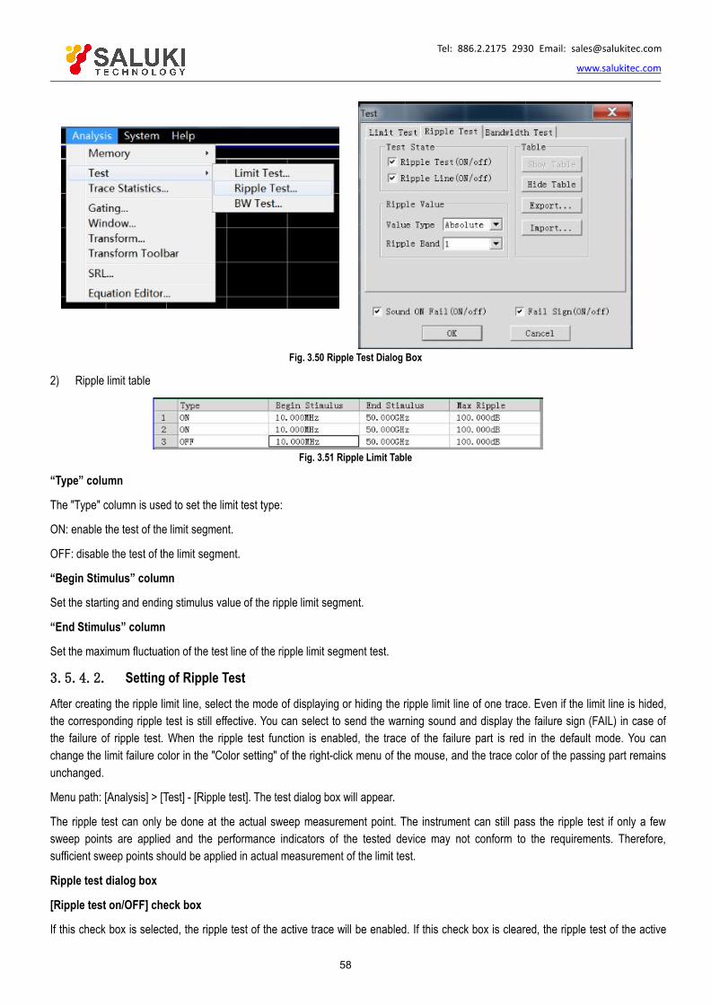
Tel: 886.2.2175 2930 Email: [email protected]
www.salukitec.com
58
Fig. 3.50 Ripple Test Dialog Box
2) Ripple limit table
Fig. 3.51 Ripple Limit Table
“Type” column
The "Type" column is used to set the limit test type:
ON: enable the test of the limit segment.
OFF: disable the test of the limit segment.
“Begin Stimulus” column
Set the starting and ending stimulus value of the ripple limit segment.
“End Stimulus” column
Set the maximum fluctuation of the test line of the ripple limit segment test.
3.5.4.2. Setting of Ripple Test
After creating the ripple limit line, select the mode of displaying or hiding the ripple limit line of one trace. Even if the limit line is hided,the corresponding ripple test is still effective. You can select to send the warning sound and display the failure sign (FAIL) in case ofthe failure of ripple test. When the ripple test function is enabled, the trace of the failure part is red in the default mode. You canchange the limit failure color in the "Color setting" of the right-click menu of the mouse, and the trace color of the passing part remainsunchanged.
Menu path: [Analysis] > [Test] - [Ripple test]. The test dialog box will appear.
The ripple test can only be done at the actual sweep measurement point. The instrument can still pass the ripple test if only a fewsweep points are applied and the performance indicators of the tested device may not conform to the requirements. Therefore,sufficient sweep points should be applied in actual measurement of the limit test.
Ripple test dialog box
[Ripple test on/OFF] check box
If this check box is selected, the ripple test of the active trace will be enabled. If this check box is cleared, the ripple test of the active

Tel: 886.2.2175 2930 Email: [email protected]
www.salukitec.com
59
trace will be disabled.
[Ripple line on/OFF] check box
If this check box is selected, the ripple line of the active trace will be displayed on the screen. If this check box is cleared, the rippleline display of the active trace will be turned off, however, the ripple test function will not be affected.
[Sound ON Fail on/OFF] check box
If this check box is selected, the buzzer will send the warning sound in case of failure of the trace data point test.
[FAIL sign on/OFF] check box
If this check box is selected, the FAIL sign will be displayed on the screen in case of failure of the trace data point test.
[Show table] button
Click it to display and edit the ripple table. If the ripple table is opened, this button will be disabled.
[Hide table] button
Click it to close the ripple table display. If the ripple table is closed, this button will be disabled. [Export...] button
Click it and the storage dialog box will pop up. You can select the storage path, and the file will be saved in the "*.csv" format.
[Import...] button
Click it and the storage dialog box will pop up. Select the storage path of the file to be opened, and the file will be opened in the "*.csv"format.
[value type] drop-down option box
Click this drop-down option box to select the limit test type: none, absolute value and allowance. The default value is the absolutevalue after start-up of the instrument.
[Ripple Band] drop-down option box
Click the drop-down option box to select the number of ripple limit segments to be opened. At most 12 segments can be opened.
3.5.4.3. Display of Ripple Test ResultsIf the measurement results of ripple test conform to the requirements, "PASS" will be displayed in the upper left corner of the screen;otherwise, "FAIL" will be displayed. "PASS" and "FAIL" of each trace will be respectively displayed if several tracks are tested at thesame time. The stimulus ranges of different ripple limit segments are allowed to be overlapping, and various ripple limits can be set.
Fig. 3.52 Ripple Test Results

Tel: 886.2.2175 2930 Email: [email protected]
www.salukitec.com
60
3.5.5. Bandwidth TestThe bandwidth test function is mainly used to test the bandwidth of the band pass filter.
The signal peak within the pass band can be found in the bandwidth test. Two points are respectively located at the specific amplitudeon both side of the pass band. The amplitude amplitude is lower than the signal peak and can be adjusted by setting the NdB point(default setting: 3dB). The frequency range between the two points is the bandwidth of the tested filter.
The minimum bandwidth and maximum bandwidth allowed by the user can be set before the bandwidth test. The actual bandwidth willbe automatically compared with the above two values. In case of nonconformity, the FAIL information will be provided on the screen orthe sound will be utters, so that the user can intuitively check whether the properties of the tested device conforms to therequirements.
3.5.5.1. Enabling and Setting of Bandwidth TestSet the bandwidth threshold (NdB point), maximum bandwidth and minimum bandwidth before the bandwidth test. Several tracks canbe set.
1) Menu path: [Analysis] > [Test] > [BW test]. The test dialog box will appear.
2) Tick the [Bandwidth test on/OFF] check box in the dialog box to enable the bandwidth test.
3) Tick the [Bandwidth Value on/OFF] check box in the dialog box to display the tested bandwidth on the screen.
4) Tick the [Bandwidth Marker on/OFF] check box in the dialog box. The bandwidth location mark will be displayed on the screen.
5) Click the [NdB point] box to set the bandwidth threshold.
6) Click the [Min bandwidth] box to set the minimum bandwidth.
7) Click the [Max bandwidth] box to set the maximum bandwidth.
8) Tick the [Sound ON Fail on/OFF] check box in the dialog box. The sound prompt will be provided in case of failure of thebandwidth test.
9) Tick the [FAIL sign on/OFF] check box in the dialog box. The FAIL prompt will be provided in case of failure of the bandwidth test.
10) Click [OK]. Thus the bandwidth test setting is completed.
Fig. 3.53 Dialog Box of Bandwidth Test
3.5.5.2. Display of Bandwidth Test ResultsBandwidth test results will be displayed in the upper left corner of the trace. If the test results are acceptable, "ASS" will be displayed.
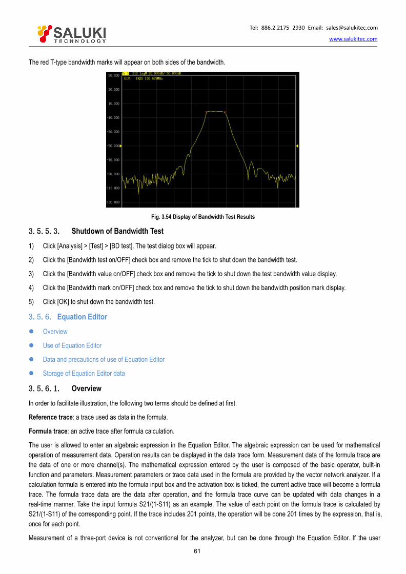
Tel: 886.2.2175 2930 Email: [email protected]
www.salukitec.com
61
The red T-type bandwidth marks will appear on both sides of the bandwidth.
Fig. 3.54 Display of Bandwidth Test Results
3.5.5.3. Shutdown of Bandwidth Test
1) Click [Analysis] > [Test] > [BD test]. The test dialog box will appear.
2) Click the [Bandwidth test on/OFF] check box and remove the tick to shut down the bandwidth test.
3) Click the [Bandwidth value on/OFF] check box and remove the tick to shut down the test bandwidth value display.
4) Click the [Bandwidth mark on/OFF] check box and remove the tick to shut down the bandwidth position mark display.
5) Click [OK] to shut down the bandwidth test.
3.5.6. Equation Editor Overview
Use of Equation Editor
Data and precautions of use of Equation Editor
Storage of Equation Editor data
3.5.6.1. Overview
In order to facilitate illustration, the following two terms should be defined at first.
Reference trace: a trace used as data in the formula.
Formula trace: an active trace after formula calculation.
The user is allowed to enter an algebraic expression in the Equation Editor. The algebraic expression can be used for mathematicaloperation of measurement data. Operation results can be displayed in the data trace form. Measurement data of the formula trace arethe data of one or more channel(s). The mathematical expression entered by the user is composed of the basic operator, built-infunction and parameters. Measurement parameters or trace data used in the formula are provided by the vector network analyzer. If acalculation formula is entered into the formula input box and the activation box is ticked, the current active trace will become a formulatrace. The formula trace data are the data after operation, and the formula trace curve can be updated with data changes in areal-time manner. Take the input formula S21/(1-S11) as an example. The value of each point on the formula trace is calculated byS21/(1-S11) of the corresponding point. If the trace includes 201 points, the operation will be done 201 times by the expression, that is,once for each point.
Measurement of a three-port device is not conventional for the analyzer, but can be done through the Equation Editor. If the user

Tel: 886.2.2175 2930 Email: [email protected]
www.salukitec.com
62
expects to obtain a logarithmic formula trace, the following expression can be used: S21+S23- S13. However, the data used in theEquation Editor are plural data with no format requirements. The user needs to enter the following formula: S21*S23/S13. After theformula is entered, Eq=S12*S23/S13 will be displayed on the current active trace of the vector network analyzer.
Fig. 3.55 Dialog Box of Equation Editor
3.5.6.2. Use of Equation Editor1) Open the Equation Editor dialog box.
Click the [Analysis] > [Equation Editor] in the menu of the vector network analyzer to open the Equation Editor dialog box, as shown inFig. 3.56.
Fig. 3.56 Equation Editor Menu
2) How to enter the formula in the Equation Editor dialog box
a) Function input
Click the function list under [Function and constants] in Fig. 3.55 and enter the function in the formula input box, or directly enter thefunction through the keyboard.
b) Operator input
Click the operator list under [Operator] and enter the operator in the formula input box, or enter the operator through the keyboard.
c) Trace and channel input
Click the mouse to enter the trace and channel parameters among the options in the drop-down list of [Trace] or [Channel parameters],as the formula parameters or variables, or enter the operator through the keyboard.
d) Data input
Enter the numbers through the number keys on the right side, or enter the operator through the keyboard.

Tel: 886.2.2175 2930 Email: [email protected]
www.salukitec.com
63
3) “Activation” check box
The "activation" check box is ticked in the default mode. The formula entered by the user will be judged only when this check box isticked. If the formula is applicable to calculation, operation will be started. The expression Eq=XXX of the current formula will bedisplayed on the active trace of the current active window of the vector network analyzer. If this check box is not ticked, operation willnot be started no matter whether the entered expression is applicable to calculation. In addition, if this check box is ticked but theentered formula is not applicable to calculation (such as the case of "2+1+"), the check box will be gray.
4) Formula saving and deleting
Click [Save formula] to save any expression entered by the user in the formula input box, the formula will be saved in the drop-downmenu of the formula input box. Click the right drop-down arrow of the formula input box and select the formula in the drop-down list.
In addition, the user can click [Delete formula] to delete the formula in the formula input box.
5) Backspace button
[<-Backspace]: used to delete one character in front of the marker. If there is no character on the left side, the marker position willremain unchanged.
6) Leftward and rightward movement of marker
[<-]: used to move the current marker left for one character but not to delete the left character. If there is no character on the left side,the marker position will remain unchanged.
[->]: used to move the current marker right for one character but not to delete the right character. If there is no character on the rightside, the marker position will remain unchanged.
7) Selection of functions and variables
The built-in function library is set in the default mode, including the commonly used formulas and constants to be selected by clicking.The functions/constants are shown in Table 3.10. If the parameter of one function is of plural type, the scalar can be used as theparameter. The scalar is a plural, with 0 as the imaginary part.
Table 3.10 List of Functions/Constants
acos(scalar a) Return to the ACOS value of the parameter a in radian. The parameter a is a scalar.asin(scalar a) Return to the ASIN value of the parameter a in radian. The parameter a is a scalar.atan(scalar a) Return to the Atan value of the parameter a in radian. The parameter a is a scalar.
atan2 Return to the phase of the plural a in radian. Two parameter types can be applied:
atan2 (complex a): return to the phase in radian. The parameter a is a scalar.
atan2 (scalar a and scalar b): return to the phase in radian. The parameter a and b are scalars.
conj(complex a) Return to the conjugate complex of the plural a.cos(complex a) Calculate the cosine value of the plural a. The real part and imaginary part of a are in radian.
cpx(scalar a,scalar b) Return to a plural (a+jb). The parameter a and b are scalars.getNumPoints() Return to the number of the current sweep points.im(complex a) Return to the imaginary part of the parameter a.
kfac(rComplex a,rComplex b,
rComplex c,
Return value k = (1-|a|^2-|d|^2+|a*d-b*c|^2)/(2*|b*c|). The parameter a, b, c and d are plurals.
ln(complex a) Return to the natural logarithm of the plural a.log10(complex a) Return to the logarithm of 10 corresponding to the plural a.mag(complex a) Return to the modulus of the plural a. The parameter a is a plural.

Tel: 886.2.2175 2930 Email: [email protected]
www.salukitec.com
64
mu1(complex a,complex b,complex c,complex d)
Return value mu1 = (1-|a|^2)/(|d-conj(a)*(a*d-b*c)|+|b*c|). The parameter a, b, c and d are plurals.
mu2(complex a,complex b,complex c,complex d)
Return value mu2 = (1-|d|^2)/(|a-conj(d)*(a*d-b*c)|+|b*c|). The parameter a, b, c and d are plurals.
phase(complex a) Return to atan2 (a), i.e. calculation phase, in radian. The parameter is a plural.PI Constant Pi, 3.141592.
re(complex a) Return to the real part of the plural a. The plural a is a plural.sin(complex a) Return to the sine value of the plural a. The parameter a is a plural, in radian.sqrt(complex a) Return to the square root of the modulus of the plural a. The parameter a is a plural.tan(complex a) Return to the tangent value of the plural a. The parameter a is a plural, in radian.
8) Operator selection
Operations are shown in Table 3.11. The user can click the mouse to select the required operator, such as four basic operators, i.e."+","-", "*" and "/", as well as the left bracket and right bracket. In addition, the Equation Editor also supports direct input of plural data foroperation. To enter the plural constant 2+j3, the user should enter <2:3> into the Equation Editor to indicate the plural constant 2+j3.To enter the (2+j3)*S11, the user should enter the expression <2:3>*S11 for operation.
Table 3.11 List of Operators
+ Addition operator- Subtraction operator* Multiplication operator/ Division operator( Left bracket) Right bracket, Comma, used to separate several parameters.< Start symbol to enter the plural.: Used to separate the real part and imaginary part of the plural.> Ending symbol to enter the plural.
9) Trace data
The user can select the trace or trace data in the list below, but the current active trace cannot be selected.
10) Channel parameter data
The user can only select the S-parameter of the current active channel as the parameter data of the entered expression.
11) Number key zone
The user can enter numbers by clicking number keys in the number key zone, the positive and negative symbol by clicking [+/-] andthe decimal point by clicking [•].
3.5.6.3. Data and Precautions of Use of Equation Editor
The data of each point of the formula trace can be calculated according to the data of the corresponding point on the reference trace.If the trace includes 201 points, the calculation will be done 201 times by the formula, i.e. Once for each data point. If the current traceis Tr4 and the formula is Tr2+S11, Tr4 will be the formula trace. Tr1 and S11 are the reference tracks of the formula trace. In addition,the current active trace Tr4 in the display window of the vector network analyzer will be displayed as Tr4Eq=Tr2+S11. As shown in Fig.3.57.
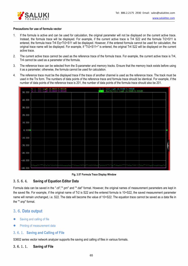
Tel: 886.2.2175 2930 Email: [email protected]
www.salukitec.com
65
Precautions for use of formula vector
1. If the formula is active and can be used for calculation, the original parameter will not be displayed on the current active trace.Instead, the formula trace will be displayed. For example, if the current active trace is Tr4 S22 and the formula Tr2+S11 isentered, the formula trace Tr4 Eq=Tr2+S11 will be displayed. However, if the entered formula cannot be used for calculation, theoriginal trace name will be displayed. For example, if "Tr2+S11+" is entered, the original Tr4 S22 will be displayed on the currentactive trace.
2. The current active trace cannot be used as the reference trace of the formula trace. For example, the current active trace is Tr4,Tr4 cannot be used as a parameter of the formula.
3. The reference trace can be selected from the S-parameter and memory tracks. Ensure that the memory track exists before usingit as a parameter; otherwise, the formula cannot be used for calculation.
4. The reference trace must be the displayed trace if the trace of another channel is used as the reference trace. The track must beused in the Trx form. The numbers of data points of the reference trace and formula trace should be identical. For example, if thenumber of data points of the reference trace is 201, the number of data points of the formula trace should also be 201.
Fig. 3.57 Formula Trace Display Window
3.5.6.4. Saving of Equation Editor DataFormula data can be saved in the ".cti","*.prn" and "*.dat" format. However, the original names of measurement parameters are kept inthe saved file. For example, if the original name of Tr2 is S22 and the entered formula is 10+S22, the saved measurement parametername will remain unchanged, i.e. S22. The data will become the value of 10+S22. The equation trace cannot be saved as a data file inthe "*.snp" format.
3.6.Data output Saving and calling of file
Printing of measurement data
3.6.1. Saving and Calling of FileS3602 series vector network analyzer supports the saving and calling of files in various formats.
3.6.1.1. Saving of File
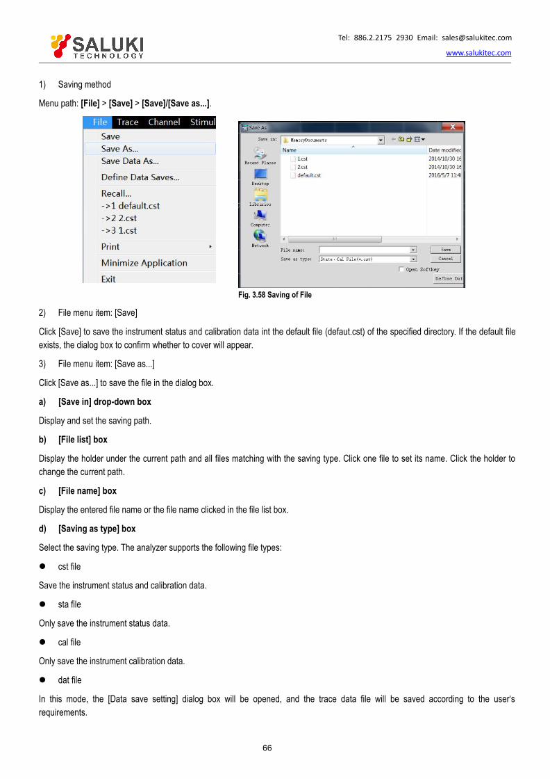
Tel: 886.2.2175 2930 Email: [email protected]
www.salukitec.com
66
1) Saving method
Menu path: [File] > [Save] > [Save]/[Save as...].
Fig. 3.58 Saving of File
2) File menu item: [Save]
Click [Save] to save the instrument status and calibration data int the default file (defaut.cst) of the specified directory. If the default fileexists, the dialog box to confirm whether to cover will appear.
3) File menu item: [Save as...]
Click [Save as...] to save the file in the dialog box.
a) [Save in] drop-down box
Display and set the saving path.
b) [File list] box
Display the holder under the current path and all files matching with the saving type. Click one file to set its name. Click the holder tochange the current path.
c) [File name] box
Display the entered file name or the file name clicked in the file list box.
d) [Saving as type] box
Select the saving type. The analyzer supports the following file types:
cst file
Save the instrument status and calibration data.
sta file
Only save the instrument status data.
cal file
Only save the instrument calibration data.
dat file
In this mode, the [Data save setting] dialog box will be opened, and the trace data file will be saved according to the user‘srequirements.
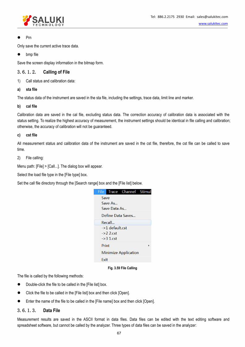
Tel: 886.2.2175 2930 Email: [email protected]
www.salukitec.com
67
Prn
Only save the current active trace data.
bmp file
Save the screen display information in the bitmap form.
3.6.1.2. Calling of File
1) Call status and calibration data:
a) sta file
The status data of the instrument are saved in the sta file, including the settings, trace data, limit line and marker.
b) cal file
Calibration data are saved in the cal file, excluding status data. The correction accuracy of calibration data is associated with thestatus setting. To realize the highest accuracy of measurement, the instrument settings should be identical in file calling and calibration;otherwise, the accuracy of calibration will not be guaranteed.
c) cst file
All measurement status and calibration data of the instrument are saved in the cst file, therefore, the cst file can be called to savetime.
2) File calling:
Menu path: [File] > [Call...]. The dialog box will appear.
Select the load file type in the [File type] box.
Set the call file directory through the [Search range] box and the [File list] below.
Fig. 3.59 File Calling
The file is called by the following methods:
Double-click the file to be called in the [File list] box.
Click the file to be called in the [File list] box and then click [Open].
Enter the name of the file to be called in the [File name] box and then click [Open].
3.6.1.3. Data FileMeasurement results are saved in the ASCII format in data files. Data files can be edited with the text editing software andspreadsheet software, but cannot be called by the analyzer. Three types of data files can be saved in the analyzer:

Tel: 886.2.2175 2930 Email: [email protected]
www.salukitec.com
68
1) dat file
The "dat" file is used for saving measurement data of the active trace or all tracks in the formatted or unformatted form. Define thedata saving mode in the [Data save setting] dialog box.
The "at" file is saved by the following methods:
a) Menu path: [File] > [Save as...]. The [Save as...] dialog box will appear.
b) Set the file saving type as the data file (*.dat) in the [Saving type] box.
c) Set the saving directory in the [Save in] box and [File list] box.
d) Set the name of the file to be saved in the [File name] box.
e) Click [Save]. The [Data save setting] dialog box will appear.
f) Set the contents and format of the file to be saved. Click [Formatted data] or [Unformatted] to save the data file. Close the dialogbox.
[Save contents] zone
Define the trace data to be saved into the file.
a) [Default] radio box
Save the data of active tracks in all windows.
b) [One trace] radio box
Save the data of the current active trace.
c) [Window trace] radio box
Save the data of all tracks in the current active window.
d) [All tracks] radio box
Save the data of all tracks.
[Saving format] zone
a) [Auto] radio box
Save the trace data according to the actual display format.
b) [Log] radio box
Save the trace data in the logarithmic amplitude format.
c) [Linear format] radio box
Save the trace data in the linear amplitude format.
d) [Real part format] radio box
Save the trace data in the real part format.
e) [Imaginary part format] radio box
Save the trace data in the imaginary part format.
[Formatted data] button
Save the trace data in the format set in the [Saving format] zone.
[Unformatted] button

Tel: 886.2.2175 2930 Email: [email protected]
www.salukitec.com
69
Save the trace data in the real/imaginary part format.
2) snp (s1p and s2p) file
The “snp" file is a kind of data output file. It can be called by the CAE (computer aided engineering) software (such as ADS of Agilent),but cannot be called by the analyzer. The “s1p" file is used to save the characteristics of single-port devices, only including one Sparameter (S11 or S22). The "s2p" file is used to save the characteristics of 2-port devices, including four S parameters. If the full2-port correction is started, four S parameters will be saved in the "s2p" file. If the full 2-port correction is shut down, measurementdata will be saved in the "s2p" file as much as possible. Example: if the full 2-port correction is shut down, the current active trace isS11, but S21 is still measured in the channel, measurement results of S11 and S21 will be saved in the "s2p" file. As no effectivemeasurement data of S22 and S12 are provided, the corresponding data in the "s2p" file are 0.
The “snp" file is saved by the following method:
a) Menu path: [File] > [Save] > [Save as...]. The [Save as] dialog box will appear.
b) Set the saving type as the data file (*.s1p or *.s2p) in the [Saving type] box.
c) Set the saving directory in the [Save in] box and [File list] box.
d) Set the file name in the [File name] box.
e) Click [Save] to save data.
3) prn file
The prn file is used to save the measurement data of the active trace in lines and rows. Each line corresponds to one measurementpoint. The first row corresponds to the stimulus value, while the second row corresponds to the response value. The format is asfollows:
S11 LogMag
LIN_SWEEP (Hz) LOG_FORMAT (dB)
3.000000e+005 -9.232986e+000
7.502250e+008 -3.219671e-001
1.500150e+009 -6.892332e+000
2.250075e+009 -1.146303e+000
3.000000e+009 -1.245240e+001
The “prn" file is saved in the following method:
Menu path: [File] > [Save] > [Save as...]. The [Save as...] dialog box will appear.
Set the saving type as the list file (*.prn) in the [Saving type] box.
Set the saving directory in the [Save in] box and [File list] box.
Set the file name in the [File name] box. Click [Save] to save the file. Close the dialog box.
3.6.2. Printing of Measurement ContentsThe analyzer supports the output of measurement contents through the printer or printing into the specified file. The local ornetwork printer can be used. The printer can be of parallel, serial or USB interface type. Add the printer in the WINDOWSoperating system.
3.6.2.1. Print Setup Method of print setting
Menu path: [File] > [Print] > [Page Setup]. Then the page setup dialog box will appear.

Tel: 886.2.2175 2930 Email: [email protected]
www.salukitec.com
70
Fig. 3.60 Print Setting
[Page Setup] dialog box
1) [Window info] zone
a) [Print] check box
If this check box is selected, the window trace information will be printed. If this check box is cleared, the window trace information willnot be printed. The following two check boxes are effectively only when the above check box is selected.
b) [One window per page] check box
If this check box is selected, only the information of one window will be printed. If this check box is cleared, the information of allwindows will be printed continuously, with no page breaks.
c) [Print active window] radio box
If this box is selected, only the information of the current active window will be printed.
d) [Print all windows] radio box
If this box is selected, only the information of the current active window will be printed.
2) [Other info] zone
a) [Print] check box
If this check box is selected, the channel setting information will be printed. The following check boxes are effectively only when thischeck box is selected.
b) [Segment table], [Limit table], [marker table], [Channel statue] and [Time] check box
Select to print the corresponding information.
3) [Separately print window and other information] check box
If this check box is selected, the window and other information will be printed separately. If this check box is cleared, the aboveinformation will be printed together.
3.6.2.2. Printing
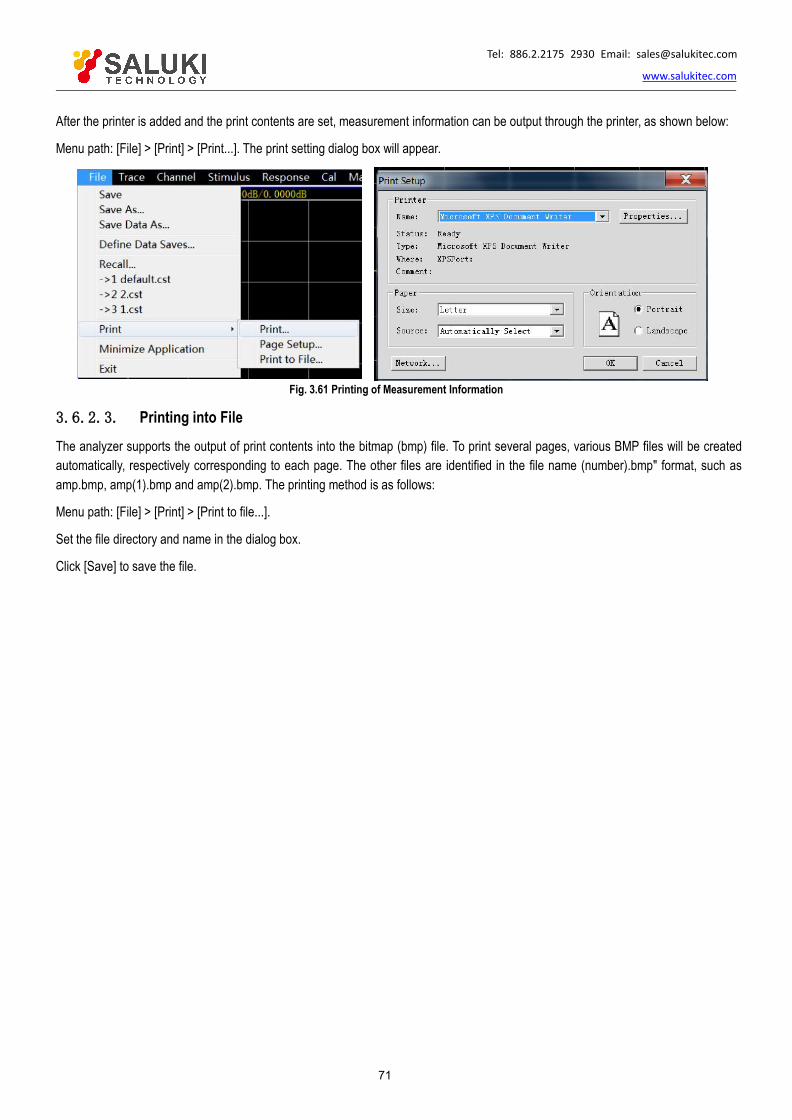
Tel: 886.2.2175 2930 Email: [email protected]
www.salukitec.com
71
After the printer is added and the print contents are set, measurement information can be output through the printer, as shown below:
Menu path: [File] > [Print] > [Print...]. The print setting dialog box will appear.
Fig. 3.61 Printing of Measurement Information
3.6.2.3. Printing into File
The analyzer supports the output of print contents into the bitmap (bmp) file. To print several pages, various BMP files will be createdautomatically, respectively corresponding to each page. The other files are identified in the file name (number).bmp" format, such asamp.bmp, amp(1).bmp and amp(2).bmp. The printing method is as follows:
Menu path: [File] > [Print] > [Print to file...].
Set the file directory and name in the dialog box.
Click [Save] to save the file.

Tel: 886.2.2175 2930 Email: [email protected]
www.salukitec.com
72
4. Measurement setupsThis chapter mainly describes the operation of S3602 series network analyzers in measurement, creation of the measurement ofthe known status by analyzer resetting, selection of Measurement setups, adjustment of the analyzer display so as to betterobserve measurement results, specifically including:
Resetting of analyzer
Selection of measurement parameter
Setting of frequency range
Setting of signal power level
Setting of sweep
Trigger mode
Setting of data format and scale
Observation of multiple tracks and opening of multiple channels
Setting of analyzer display
4.1.Resetting of Analyzer
Default reset state
User reset state
Resetting of analyzer
4.1.1. Default Reset StatePress the [Reset] on the front panel to return to the known default state, i.e. reset state. The reset state is set as follows:
1) Measurement parameter: S11
2) Frequency setting:
a) Starting frequency: 10MHz
b) Ending frequency: 13.5GHz/26.5GHz/43.5GHz/50GHz/67GHz
c) CW frequency: 2GHz
3) Power setting:
a) Test port power: -5dBm
b) Coupling port power: open
c) Attenuation: automatic
d) Attenuation values: 0dB
e) Power slope: closed
f) Slope: 0dB/GHz
4) Sweep setting:
a) sweep type: linear frequency
b) sweep time: automatic

Tel: 886.2.2175 2930 Email: [email protected]
www.salukitec.com
73
c) Number of sweep points: 201
5) Segment sweep setting:
a) Number of open segments: 1
b) Starting frequency: 10MHz
c) Ending frequency: 13.5GHz/26.5GHz/43.5GHz/50GHz/67GHz
d) Number of points: 21
e) Power: -5dBm
f) Intermediate frequency bandwidth: 1kHz
6) Trigger setting:
a) Trigger source: internal
b) Trigger type: continuous scanning
7) Display format:
Format: logarithmic amplitude
The details of various formats are shown in Table 4.1.
Table 4.1 Default Format Setting of S3602 Series Vector Network Analyzers
Format Scale Reference position Reference value
Logarithmic amplitude ≤10 dB 5 0dB
phase 45o 5 0o
Group delay 10ns 5 10fs
Linear amplitude 100mU 5 500mU
Standing wave ratio 1U 5 6U
Real part 2U 5 0U
Imaginary part 2U 5 0U
Polar coordinate 1U None 1U
Smith chart 1U None 1U
8) Response setting:
a) Number of channels: 1
b) Intermediate frequency bandwidth: 1kHz
c) Average: closed
d) Average factor: 1
e) Smoothing: closed
f) Smoothing factor: 2.49% of the value range
g) Electrical delay: 0s
h) Speed factor: 1

Tel: 886.2.2175 2930 Email: [email protected]
www.salukitec.com
74
i) Phase shift: 0°
j) Trace display: data
9) Calibration setting:
a) Correction: closed
b) Interpolation: open
c) Calibration type: none
d) Calibration kit number: current calibration kit number
e) System impedance: 50Ω
f) Port extension: closed
g) Port extension value: 0s
10) Marker setting:
a) Initial frequency: full range of center frequency
b) Reference marker R: closed
c) Discrete marker: closed
d) Format: trace format
e) Type: standard
f) Marker search type: minimum
g) Search domain: full bandwidth
h) Marker table: empty
11) Limit test setting:
a) Limit test: closed
b) Limit line display: closed
c) FAIL sound warning: closed
12) Limit table setting:
a) Type: OFF
b) Initial stimulus: 10MHZ
c) Ending stimulus: 13.5GHz/26.5GHz/43.5GHz/50GHz/67GHz
d) Initial response: -100dB
e) Ending response: 100dB
13) Time domain transformation setting (optional):
a) Time domain transformation: closed
b) Transformation mode: bandpass
c) Transformation start: -5ns
d) Transformation end: 5ns
e) Kaiser window β factor: 6.0

Tel: 886.2.2175 2930 Email: [email protected]
www.salukitec.com
75
f) Gate state: closed
g) Gate starting value: -5ns
h) Gate ending value: 5ns
i) Gate shape: standard
j) Gate type: bandpass
14) Full display setting:
a) Trace state: open
b) Frequency/stimulus: open
c) marker reading: open
d) Status bar: closed
4.1.2. User Reset StateThe analyzer can be reset into the known default status or user-defined status. In the default mode, the analyzer is reset into thedefault status. It can be reset into the user-defined status by means of setting. Specific steps of setting the user reset status are asfollows.
1) Menu path: [System] > [Define user state...]. Then the [Define user state...] dialog box will appear.
2) Click [Enable user reset status] and tick the check box.
Notes:
a) If you tick [Save final status as user preset], the final status before exiting the program will be saved as the user reset state.
b) Click [Save current status as user status]. Then the current settings of the analyzer will be saved as the user reset status.
c) To use the known status, click [Load exist file as user reset status]. Select the status in the dialog box, and open the file. Thenthe selected file will be used as the user reset status file of the analyzer.
Fig. 4.1 Definition of User Reset Status
4.1.3. Resetting of AnalyzerMenu path: [System] > [Reset]
If the user reset state has been set, click [User reset].

Tel: 886.2.2175 2930 Email: [email protected]
www.salukitec.com
76
Fig. 4.2 Resetting of Analyzer
[Reset] shortcut key
The [Reset] shortcut key is set in the functional key zone and shortcut menu bar.
4.2.Selection of Measurement Parameter
The following parameters can be set in an S3602 series vector network analyzer to measure the electrical characteristics ofdevices.
S parameter (fixed ratio)
Any ratio (custom ratio for measurement)
Non-ratio power measurement (absolute power measurement)
S parameter
Any ratio
Non-ratio power measurement
Change of trace measurement type
4.2.1. Parameter S
1) Overview of Parameter S
The parameter S (scattering parameter) is used to describe the change of input signal and the reflection and transmissioncharacteristics of the tested device. The S-parameter is shown in the prescribed digit row, and indicates the proportion of twocomplex vectors, i.e. Soutput/input, including the amplitude and phase information. The output refers to the output signal port numberof the tested device, and the input refers to the input signal port number of the tested device. The analyzer is equipped with fourtest ports to test single-port, double-port, three-port and four-port devices.
For example, when one 2-port device is connected to Port 1 and 2, four parameters (S) can be measured at the same time.
In this case, the four parameters (S) of the 2-port device are respectively S11, S12, S21 and S22. Fig. 4.3 further shows theparameter S, where:
a refers to the stimulus signal from the input to tested device.
b refers to the reflection and transmission signal (response signal) of the tested device.
The parameter S is a plural linear value. The measurement accuracy depends on the indicators of the calibrator and the adopted

Tel: 886.2.2175 2930 Email: [email protected]
www.salukitec.com
77
technology of measurement connection, and is also associated with the connection of the non- measurement port (non-excitedport).
2) Application of parameter S
The following parameters can be measured with S.
a) Reflection measurement: SXX (X=1, 2, 3, 4)
1. Return loss2. Standing wave ratio (SWR)3. reflection coefficient4. Impedance5. S11, S22, S33 and S44
b) Transmission measurement: SXY (X=1, 2, 3, 4; Y=1, 2, 3, 4; X≠Y)
1. Insertion loss2. Transmission coefficient3. Group delay4. SXY
The measurement of the 2-port device with Port 1 and 2 is taken as an example below to introduce the parameter S.
Fig. 4.3 Definition of Parameter S
3) New S measurement trace
Menu path: [Trace] > [New trace]. Click the S-parameter in the dialog box.

Tel: 886.2.2175 2930 Email: [email protected]
www.salukitec.com
78
Fig. 4.4 Definition of Parameter S
4) [New trace] dialog box
a) [S-Parameter] zone
Select the S parameter measurement trace to be created.
b) [Receiver] button
Open the dialog box to create any ratio or non-ratio power measurement trace.
c) [Balance parameter] button
Open the dialog box to create the balance parameter measurement trace.
d) [Channel selection] box
Select the channel where the new trace is located.
e) [Create in new window] check box
If this check box is selected, a trace will be created in the new window. If this check box is cleared, a trace will be created in thecurrent active window.
4.2.2. Any RatioThe input signal and reference signal are selected from the receiver A, B, C, D, R1, R2, R3 or R4 for ratio measurement.
1) Create measurement trace of any ratio
Menu path: [Trace] > [New trace]. Click “Receiver" in the dialog box.
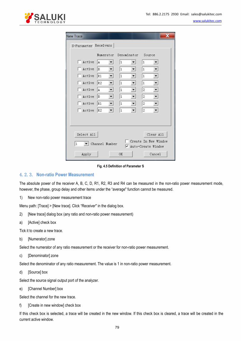
Tel: 886.2.2175 2930 Email: [email protected]
www.salukitec.com
79
Fig. 4.5 Definition of Parameter S
4.2.3. Non-ratio Power MeasurementThe absolute power of the receiver A, B, C, D, R1, R2, R3 and R4 can be measured in the non-ratio power measurement mode,however, the phase, group delay and other items under the “average" function cannot be measured.
1) New non-ratio power measurement trace
Menu path: [Trace] > [New trace]. Click “Receiver" in the dialog box.
2) [New trace] dialog box (any ratio and non-ratio power measurement)
a) [Active] check box
Tick it to create a new trace.
b) [Numerator] zone
Select the numerator of any ratio measurement or the receiver for non-ratio power measurement.
c) [Denominator] zone
Select the denominator of any ratio measurement. The value is 1 in non-ratio power measurement.
d) [Source] box
Select the source signal output port of the analyzer.
e) [Channel Number] box
Select the channel for the new trace.
f) [Create in new window] check box
If this check box is selected, a trace will be created in the new window. If this check box is cleared, a trace will be created in thecurrent active window.

Tel: 886.2.2175 2930 Email: [email protected]
www.salukitec.com
80
g) [Automatically create window] check box
If this check box is ticked and the number of tracks in the window exceeds 8, excessive tracks will be automatically created in anew window.
If this check box is cleared and the number of tracks in the window exceeds 8, excessive tracks will not be created.
4.2.4. Measurement mode of trace changeThe trace must be activated before setting and modification.
1) Change the trace activation status
Click the [Trace status] button in the window. The corresponding trace will be activated.
Fig. 4.6 Change of trace Activation Status
2) Change the measurement parameter of the activated trace
Menu path: [Response] > [Measure].
The measure sub-menu will appear. Or, right-click the trace title bar, and click [Measure] in the menu, as shown in Fig. 4.7.
Fig. 4.7 Setting of Parameter S Measurement Mode of Activated Trace
4.3.Setting of Frequency Range
Frequency range: 10MHz-13.5GHz/26.5GHz/43.5GHz/50GHz/67GHz
Frequency resolution: 1Hz
1) Two ways of frequency range setting
a) Specify the start/stop frequency.
b) Specify the center frequency and frequency span.
2) Setting of start and Stop frequency
Menu path: [Stimulus] > [Frequency]

Tel: 886.2.2175 2930 Email: [email protected]
www.salukitec.com
81
Fig. 4.8 Setting of Start / Stop Frequency
3) Setting of center frequency and frequency span
Menu path: [Stimulus] > [Freq]
Fig. 4.9 Setting of Center Frequency and Frequency Span
[Frequency] shortcut key
The frequency can be rapidly set with the [Frequency] shortcut key in the functional key zone of the front panel.
4.4.Setting of Signal Power Level
The power level refers to the power level of the output signal of the test port. The power level indicators of the port of S3602 seriesvector network analyzer are as follows.
Table 4.2 Power Level Indicators of Source Output Signal
Frequency range Source frequency range (dBm) Configuration
10MHz-13.5GHz/26.5GHz/43.5GHz/50GHz/67GHz -30 - +20 Standard configuration
10MHz - 13.5GHz/26.5GHz -100 - +20 Option: program-controlled step attenuator
10MHz - 43.5GHz/50GHz -90 - +20 Option: program-controlled step attenuator
1) Setting of power level
Menu path: [Stimulus] > [Power].
[Power] shortcut key is set in the functional key zone of the front panel and the shortcut menu bar.

Tel: 886.2.2175 2930 Email: [email protected]
www.salukitec.com
82
Fig. 4.10 Setting of Power Level
2) Cutoff of port power
Menu path: [Stimulus] > [Power] > [Power...].
Or, switch the power by changing the setting of the [Power ON/off] check box in the [Power] dialog box.
3) Manual setting of attenuation
Menu path: [Stimulus] > [Power] > [Power and attenuators...]. The [Power and attenuators] will appear. Click to clear the [Autoattenuation] zone check box. Click the [Attenuation] input box and enter the attenuation value.
4) Setting of power slope
Menu path: [Stimulus] > [Power] > [Power...]. The [Power] dialog box will appear. Click [Slope] check box. Click the [Slope] inputbox and enter the power slope.
5) [Power] dialog box
a) [Power ON/off] check box
If this check box is ticked, the port will normally output the power. If this check box is cleared, the port output power will be cut off.
b) [Power-port 1]
Set the power level of the port 1.
c) [Power slope] check box
Tick the [Power slope] check box and enter the slope value in the [Slope] input box to enable the power slope function.
The power slope is used to compensate the power loss of the cable and test fixture as a result of frequency increase.
If the power slope function is enabled, the output power of the test port will increase (or decrease) with the increase of sweepfrequency.
Unit of power slope: dB/GHz.
Power slope setting range: -2 to +2.
6) [Power and attenuation] dialog box
Tel: 886.2.2175 2930 Email: [email protected]
www.salukitec.com
83
a) [Power ON/off] check box
If this check box is ticked, the port will normally output the power. If this check box is cleared, the port output power will be cut off.
b) [Port Powers Coupled] check box
If the [Port Powers Coupled] check box is ticked in the default mode, the power level settings of two ports of the analyzer will beidentical. However, different power levels are required for ports in some measurement applications. For example, the power ofeach port must be set separately to measure the gain and reverse isolation of one high- gain amplifier, as the power of the inputport of the amplifier is lower than that of the output port. If the [Port Powers Coupled] check box is cleared, the power level of eachport can be set separately in the analyzer.
c) [State] bar
It is [Auto] in the default mode. In this case, the power ON/OFF state can be switched according to the measurement needs. [ON]indicates the port power is always ON, while [OFF] indicates the port power is always OFF.
d) [Port power] bar
Set the port power.
e) [Auto Range] bar
If this check box is ticked, any power level can be set within the allowable range of the instrument. If this check box is cleared, thesource power and attenuation can be set manually for certain measurement, such as the reflection amplifier (oscillator orunsteady-state amplifier) measurement. In this case, the matching source impedance (better than the return loss of 20dB) shouldbe set within a wide frequency range.
f) [Attenuator] bar
Set the attenuation.
g) [Leveling Mode] bar
Set the fixed amplitude mode, including [Internal], [Receiver] and [Open loop]. The amplitude is not fixed in the [Open loop] mode.
h) [Channel Power slope] check box
Tick the [Slope] check box and enter the slope value in the [Slope] input box to enable the power slope function. The power slopeis used to compensate the power loss of the cable and test fixture as a result of frequency increase.
If the power slope function is enabled, the output power of the test port will increase (or decrease) with the increase of sweepfrequency.
Unit of power slope: dB/GHz.
Power slope setting range: -2 to +2.
i) Attenuator Settings and power range
The programmable attenuator is used to cover the whole power range. It can adjust the power level of the tested device while thepower level of the reference path of the analyzer remains unchanged. Thus, higher accuracy and characteristic indicates and moreaccurate matching of source output signals can be realized.
The fully accurate error correction can be done at the power point for measurement calibration. If the power level is changed in thesame attenuator settings as those of measurement calibration, the accuracy of error correction is higher in ratio measurement butpoorer in non-ratio measurement.
4.5.Setting of Sweep
Sweep refers to the process of continuously measuring data points according to the stimulus values in the specified sequence.
Overview of sweep types
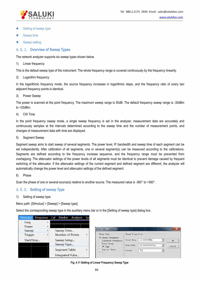
Tel: 886.2.2175 2930 Email: [email protected]
www.salukitec.com
84
Setting of sweep type
Sweep time
Sweep setting
4.5.1. Overview of Sweep Types
The network analyzer supports six sweep types shown below.
1) Linear frequency
This is the default sweep type of the instrument. The whole frequency range is covered continuously by the frequency linearity.
2) Logarithm frequency
In the logarithmic frequency mode, the source frequency increases in logarithmic steps, and the frequency ratio of every twoadjacent frequency points is identical.
3) Power Sweep
The power is scanned at the point frequency. The maximum sweep range is 50dB. The default frequency sweep range is -30dBmto +20dBm.
4) CW Time
In the point frequency sweep mode, a single sweep frequency is set in the analyzer, measurement data are accurately andcontinuously samples at the intervals determined according to the sweep time and the number of measurement points, andchanges of measurement data with time are displayed.
5) Segment Sweep
Segment sweep aims to start sweep of several segments. The power level, IF bandwidth and sweep time of each segment can beset independently. After calibration of all segments, one or several segment(s) can be measured according to the calibrations.Segments are defined according to the frequency increase sequence, and the frequency range must be prevented fromoverlapping. The attenuator settings of the power levels of all segments must be identical to prevent damage caused by frequentswitching of the attenuator. If the attenuator settings of the current segment and defined segment are different, the analyzer willautomatically change the power level and attenuator settings of the defined segment.
6) Phase
Scan the phase of one or several source(s) relative to another source. The measured value is -360° to +360°.
4.5.2. Setting of sweep Type1) Setting of sweep type
Menu path: [Stimulus] > [Sweep] > [Sweep type].
Select the corresponding sweep type in the auxiliary menu bar or in the [Setting of sweep type] dialog box.
Fig. 4.11 Setting of Linear Frequency Sweep Type
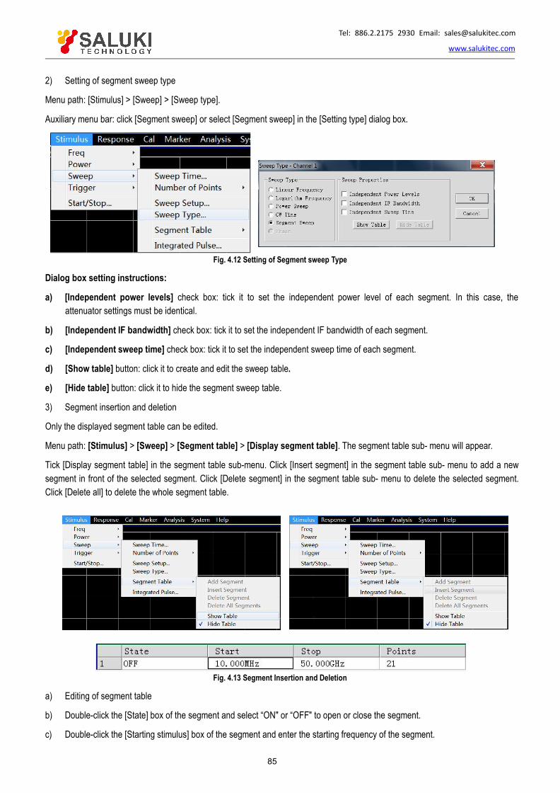
Tel: 886.2.2175 2930 Email: [email protected]
www.salukitec.com
85
2) Setting of segment sweep type
Menu path: [Stimulus] > [Sweep] > [Sweep type].
Auxiliary menu bar: click [Segment sweep] or select [Segment sweep] in the [Setting type] dialog box.
Fig. 4.12 Setting of Segment sweep Type
Dialog box setting instructions:
a) [Independent power levels] check box: tick it to set the independent power level of each segment. In this case, theattenuator settings must be identical.
b) [Independent IF bandwidth] check box: tick it to set the independent IF bandwidth of each segment.
c) [Independent sweep time] check box: tick it to set the independent sweep time of each segment.
d) [Show table] button: click it to create and edit the sweep table.
e) [Hide table] button: click it to hide the segment sweep table.
3) Segment insertion and deletion
Only the displayed segment table can be edited.
Menu path: [Stimulus] > [Sweep] > [Segment table] > [Display segment table]. The segment table sub- menu will appear.
Tick [Display segment table] in the segment table sub-menu. Click [Insert segment] in the segment table sub- menu to add a newsegment in front of the selected segment. Click [Delete segment] in the segment table sub- menu to delete the selected segment.Click [Delete all] to delete the whole segment table.
Fig. 4.13 Segment Insertion and Deletion
a) Editing of segment table
b) Double-click the [State] box of the segment and select “ON" or “OFF" to open or close the segment.
c) Double-click the [Starting stimulus] box of the segment and enter the starting frequency of the segment.
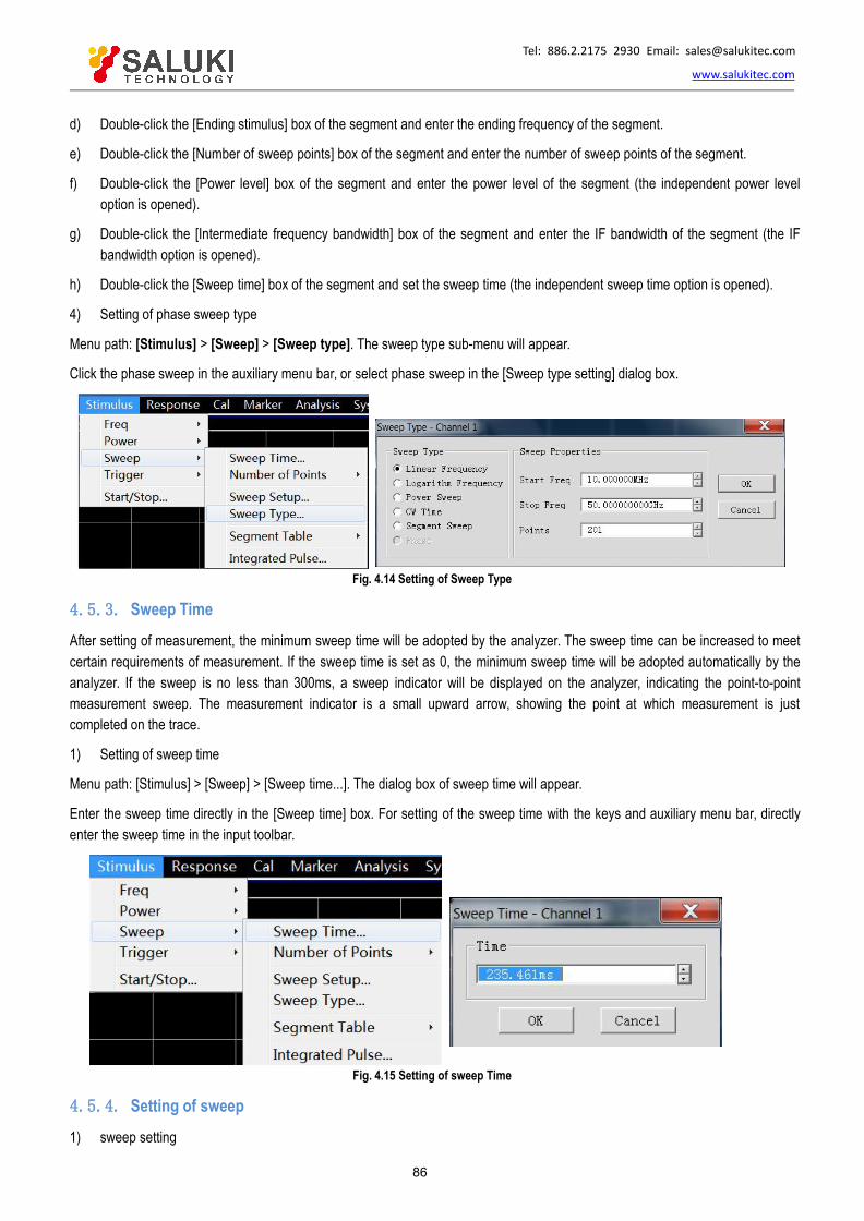
Tel: 886.2.2175 2930 Email: [email protected]
www.salukitec.com
86
d) Double-click the [Ending stimulus] box of the segment and enter the ending frequency of the segment.
e) Double-click the [Number of sweep points] box of the segment and enter the number of sweep points of the segment.
f) Double-click the [Power level] box of the segment and enter the power level of the segment (the independent power leveloption is opened).
g) Double-click the [Intermediate frequency bandwidth] box of the segment and enter the IF bandwidth of the segment (the IFbandwidth option is opened).
h) Double-click the [Sweep time] box of the segment and set the sweep time (the independent sweep time option is opened).
4) Setting of phase sweep type
Menu path: [Stimulus] > [Sweep] > [Sweep type]. The sweep type sub-menu will appear.
Click the phase sweep in the auxiliary menu bar, or select phase sweep in the [Sweep type setting] dialog box.
Fig. 4.14 Setting of Sweep Type
4.5.3. Sweep TimeAfter setting of measurement, the minimum sweep time will be adopted by the analyzer. The sweep time can be increased to meetcertain requirements of measurement. If the sweep time is set as 0, the minimum sweep time will be adopted automatically by theanalyzer. If the sweep is no less than 300ms, a sweep indicator will be displayed on the analyzer, indicating the point-to-pointmeasurement sweep. The measurement indicator is a small upward arrow, showing the point at which measurement is justcompleted on the trace.
1) Setting of sweep time
Menu path: [Stimulus] > [Sweep] > [Sweep time...]. The dialog box of sweep time will appear.
Enter the sweep time directly in the [Sweep time] box. For setting of the sweep time with the keys and auxiliary menu bar, directlyenter the sweep time in the input toolbar.
Fig. 4.15 Setting of sweep Time
4.5.4. Setting of sweep1) sweep setting

Tel: 886.2.2175 2930 Email: [email protected]
www.salukitec.com
87
Menu path: [Stimulus] > [Sweep] > [Sweep setup...]. The [Sweep setup] dialog box will appear.
Fig. 4.16 sweep Setup
2) [Sweep setup] dialog box
a) [Channel] box
Select the channel applicable to sweep setting.
b) [Stepped sweep] check box
In the stepped sweep mode, the source is tuned to a frequency point and the frequency point is measured after the specified dwelltime. Then the source is tuned to next frequency point. A device of long electrical delay can be accurately measured. If this checkbox is cleared, the analyzer may work in the analog sweep or step sweep mode, depending on the setting of the sweep time and IFbandwidth.
c) [dwell time] input box
Set the dwell time at each point before obtaining the measurement data. This is only applicable to the step scanning mode.
d) [Sweep delay] input box
Set the waiting time of the analyzer before obtaining the measurement data. It refers to the delay before measurement of the firstpoint.
e) [Quick sweep] check box
If the [Quick sweep] check box is selected, analog sweep will be started. Data are collected in the sweep process, thus reducingthe waiting time of sweep.
4.6.Trigger Mode
The trigger signal is used to enable measurement sweep of the analyzer. The sweep mode and time to stop sweep and return tothe holding state are determined by trigger settings. The vector network analyzer has high flexibility in trigger setting.
Simple trigger setting
Detailed trigger setting
[Trigger] dialog box
4.6.1. Simple Trigger SettingOnly the trigger mode of the current active channel can be set by simple trigger setting. Menu path: [Stimulus] > [Trigger]. Thetrigger sub-menu will appear. Click [Continuous], [Single] or [Hold] in the sub-menu and select the trigger mode.
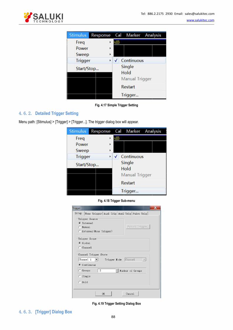
Tel: 886.2.2175 2930 Email: [email protected]
www.salukitec.com
88
Fig. 4.17 Simple Trigger Setting
4.6.2. Detailed Trigger SettingMenu path: [Stimulus] > [Trigger] > [Trigger...]. The trigger dialog box will appear.
Fig. 4.18 Trigger Sub-menu
Fig. 4.19 Trigger Setting Dialog Box
4.6.3. [Trigger] Dialog Box

Tel: 886.2.2175 2930 Email: [email protected]
www.salukitec.com
89
1) Trigger setting options
a) Trigger source zone
The source of the channel trigger signal is determined by trigger source setting of the trigger source zone. The effective triggersignal is generated when sweep is not done by the vector network analyzer. Three trigger sources can be selected: internal,manual and external. The set trigger source will be used as the trigger source of all channels.
[Internal] (default)
a) Trigger signal generation is controlled automatically by the analyzer.
b) One trigger signal is generated immediately after one measurement.
[Manual]
The manual trigger signal is generated in the following methods.
a) Click the [Manual] button in the [Trigger] dialog box.
b) Click the [Manual] item in the [Trigger] sub-menu under the [Stimulus] menu of the menu bar.
[External]
a) The trigger signal is input by [Trig In] of the BNC connector on the rear panel.
b) The signal is TTL level.
c) Level trigger: the high or low level can be set in the [Meas Trigger] dialog box.
d) The pulse duration is 1μs at and must not be longer than the sweep time (otherwise, the trigger may be enabled severaltimes).
b) Trigger Scope
The measurement channel receiving the trigger signal is determined by trigger range setting. Two types of trigger range can be set:global and channel.
[Global]
This is the default setting of the analyzer. Except the channel in the holding mode, all channels can receive the trigger signal.
[Channel]
Next channel which is not in the holding mode will receive the trigger signal. After the current channel is measured, next channelwill be selected automatically. Except the channel in the holding mode, all channels will be selected in sequence. The triggersource should be set in the manual mode to make the above setting effective. Set the [Channel] to enable the spot sweep function.
c) Channel Trigger State
The number of trigger signals to be received by one channel is determined by trigger setting. Four channel triggering states areprovided:
[Continuous]
The channel will receive a number of trigger signals. Sweep will be done continuously.
[Group]
The channel will only receive the trigger signals, the number of which is set in the [Group] input box. Sweep will be done for the settimes, and then the channel will enter the holding mode.
[Single]
The channel will receive one trigger signal. Sweep will be done once, and then the channel will enter the holding
mode.

Tel: 886.2.2175 2930 Email: [email protected]
www.salukitec.com
90
[Hold]
The channel will not receive the trigger signal, and sweep will be stopped.
[Spot] ([Trigger mode] check box)
The spot sweep mode can be selected only when the trigger source is manual or external and the trigger range is the channel. Inthe spot sweep mode, next data point will be measured in sweep after the channel receives the trigger signal. The channel willcontinuously receive the trigger signal until all measurements in the channel are done. Then next channel which is not in theholding mode will be triggered.
[Channel] ([Trigger mode] check box)
All tracks in the channel will be triggered.
[Sweep] ([Trigger mode] check box)
The sweep trigger mode can be selected only when the trigger source is manual or external and the trigger range is the channel.The tracks sharing one source port in the channel will be triggered.
2) Meas trigger options
a) Main trigger input zone
Set the nature of the external trigger signal to be received in the trigger input zone.
[Channel trigger delay]
[Delay]: Enter the delay time in the delay input box. When the instrument receives the external trigger signal, sweep will be startedafter the delay time.
[Source]
Set the external trigger signal input interface, including the BNC interface and automatic test interface (18-pin).
[Level/edge]
Set the trigger mode of the external trigger signal, including high level, low level, positive edge and negative edge.
[Accept trigger before armed]
If this item is ticked, corresponding sweep will be executed immediately after the vector network analyzer receives the trigger signal;otherwise, all the received trigger signals will be ignored.
[Ready to receive trigger prompt]
The trigger READY signal is sent by the BNC interface and automatic test interface (21-pin). High level and low level of the signalare optional.

Tel: 886.2.2175 2930 Email: [email protected]
www.salukitec.com
91
Fig. 4.20 Measurement Trigger Dialog Box
3) Auxiliary 1/2 trigger option
a) Auxiliary trigger output zone
[Enabled]
Tick the check box to open the external trigger output of the corresponding channel; otherwise, the external trigger output will beclosed.
[Polarity]
Set the polarity of the trigger output signal in the radio box: [Positive pulse] or [Negative pulse].
[Position]
Set the time to send the trigger output signal in the radio box: [Before data acquisition] or [After data acquisition].
[Pulse Duration]
Input the pulse duration of the trigger output signal in the input box.
[Enable the waiting for external equipment holding signal]
If this check box is ticked, data will not be captured until the vector network analyzer receives the specific level from the auxiliarytrigger input (1&2) connector of the rear panel. This signal indicates that the external device is ready and the network analyzer isallowed to capture data. Otherwise, the network analyzer will not wait. However, a trigger signal will be sent when the networkanalyzer is ready. This signal cannot be used to trigger the network analyzer. It is generated by the internal, manual or externalsource.
[Auxiliary trigger input]
When the network analyzer is ready, a confirmation signal will be sent to the auxiliary 1 & 2 connection port. The signal can be inthe rising edge, falling edge, high level or low level form.
[Delay]
When the network analyzer receives the holding signal, data will be captured after the corresponding delay time.

Tel: 886.2.2175 2930 Email: [email protected]
www.salukitec.com
92
Fig. 4.21 Auxiliary 1/2 Trigger Dialog Box
4) Pulse trigger options
a) Synchronous pulse input zone
Select the internal or external source to synchronize the internal pulse generator of the analyzer.
[Pulse trigger option]
Internal: the pulse generator is synchronized according to the periodic signal generated in the analyzer, and the output pulse trainperiod is determined according to the pulse repetition period in the pulse measurement interface.
External: the pulse repetition period specified by the user is ignored. One pulse train will be output once an effective external pulsesynchronization signal is detected by the analyzer. The delay and width of the pulse generator can be set respectively in the pulsemeasurement interface. The external pulse synchronization input signal will be input through the pulse input/output interface of therear panel of the analyzer. The configurable synchronization trigger signal can be input to the analyzer according to the pulsesynchronization input signal. If the level is trigger, the analyzer will output a pulse train. If the level is continuously effective, theanalyzer will continue to output another pulse train. If the edge is triggered, the analyzer will be triggered by one effective edgesignal to output a pulse train. The pulse train length is the maximum value (delay + width) in all the enabled pulse generators.
[Level/edge]
Set the characteristics of the effective external pulse synchronization input signal to be received by the analyzer: high level, lowlevel, rising edge or falling edge.
b) Receiver output zone
[Synchronize receiver to pulse]
It is used to measure the broadband synchronization pulse. When this function is enabled, the pulse generator output and datacollection are allowed to be synchronized.
[Sync Delay]
Set the delay time before collection of AD data.

Tel: 886.2.2175 2930 Email: [email protected]
www.salukitec.com
93
Fig. 4.22 Pulse Trigger Dialog Box
4.7.Setting of Data Format and Scale
The data format refers to the display of measurement data in the graphical form. Select the data format which is the most favorableto understand the characteristics of the tested device. This section introduces nine data formats and the method of scale setting soas to better display the measurement information.
Data format
Data format setting
Scale
4.7.1. Data Format1) Rectangular coordinate format
Seven of nine formats of measurement data are in the rectangular coordinate form. This format is also known as the Cartesianformat, X/Y format or linear format and is suitable to display the frequency response information of the tested device. For example,the rectangular coordinates in Fig. 4.23 show the following information.
Stimulus value (frequency, power or time) in the linear scale form on the X-axis in the default mode.
Response value corresponding to the stimulus value on the Y-axis.

Tel: 886.2.2175 2930 Email: [email protected]
www.salukitec.com
94
Fig. 4.23 Rectangular Coordinate Format
a) Logarithmic amplitude format
Display the amplitude information (no phase information).
Y-axis unit: dB
Applicable typical measurement: return loss, insertion loss and gain.
b) Phase format
Display the phase information (no amplitude information).
Y-axis unit: phase (degree)
Applicable typical measurement: linear phase offset.
c) Group delay format
Display the signal transmission time through the tested device.
Y-axis unit: time (second)
Applicable typical measurement: group delay.
d) Linear amplitude format
Only display the positive value.
Y-axis: no unit (U) in ratio measurement and milliwatt (mW) in non-ratio measurement.
Applicable typical measurement: reflection and transmission coefficient (amplitude) value and time domain transformation
e) Standing wave ratio format
Display the reflection measurement data calculated by the formula (1+ρ)/(1-ρ), where ρ is the reflection coefficient.
Effective in reflection measurement.
Y-axis: no unit.
Applicable typical measurement: standing wave ratio.
f) Real part format
Display the real part of the measurement complex.

Tel: 886.2.2175 2930 Email: [email protected]
www.salukitec.com
95
It is similar to the linear amplitude format, but both the positive value and negative value can be displayed.
Y-axis: no unit.
Applicable typical measurement: time domain and auxiliary input voltage for maintenance purposes.
g) Imaginary part format
Only display the imaginary part of measurement data.
Y-axis: no unit.
Applicable typical measurement: impedance measurement in design of matching network.
2) Polar coordinate format
The polar coordinate format shown in Fig. 4.24 includes the amplitude and phase information. The vector value can be read in thefollowing method.
a) The amplitude of any point is determined by the displacement of this point relative to the central point (or zero point). In thedefault mode, the amplitude is a linear scale, and the excircle scale is set as 1.
b) The phase of any point is determined by the angle relative to the X-axis.
c) The frequency information can only be read through the marker. The default marker format includes the real part andimaginary part. The marker dialog box can be opened in the marker/analysis menu. Other formats can be selected in theadvanced marker menu.
Fig. 4.24 Polar Coordinate Format
3) Smith chart format
Smith chart shown in Fig. 4.25 is a tool to map the reflection measurement data of the tested device into impedance.
Each point of the chart represents a complex impedance composed of the real resistance (R) and virtual reactance (±jX). Theresistance, reactance, equivalent capacitance and inductance can be read through the marker.

Tel: 886.2.2175 2930 Email: [email protected]
www.salukitec.com
96
Fig. 4.25 Smith Chart Format
a) The horizontal axis of the center of Smith chart represents the pure resistance, and the center of the horizontal axisrepresents the system impedance. The leftmost resistance on the horizontal axis is zero, indicating a short circuit. Therightmost resistance of the horizontal axis is infinite, indicating an open circuit.
b) The points on the intersecting circle of Smith chart and horizontal axis have the same resistance.
c) The points on the tangent of Smith chart and horizontal axis have the same reactance.
d) The reactance of the upper part of Smith chart is positive. Therefore, the upper part is the sensitive zone.
e) The reactance of the lower part of Smith chart is negative. Therefore, the lower part is the capacitive zone.
4.7.2. Data Format SettingMenu path: [Response] > [Format]. The format sub-menu will pop up.
Fig. 4.26 Setting of Data Format
4.7.3. ScaleThe scale refers to the scale of the vertical part of the display grid. In the polar coordinate and Smith chart format, the scale refersto the full scale of the excircle. The display mode of measurement data on the screen are determined by scale and format settings.In the log format, the scale setting range is 0.001dB/grid to 500dB/grid.

Tel: 886.2.2175 2930 Email: [email protected]
www.salukitec.com
97
1) Scale setting
Menu path: [Response] > [Scale]. The scale sub-menu will pop up.
Set the appropriate scale, reference location and reference level by clicking the corresponding input zone or keys.
Fig. 4.27 Setting of Scale
2) Scale setting dialog box
a) Scale zone
[Scale] box
Enter the set scale value.
[Automatic scale] button
Click the [Automatic scale] button. The analyzer will automatically select the vertical scale to better display the active trace in thevertical grid of the screen. The stimulus value will not be affected, and only the scale value and reference value are changed.
i. An appropriate scale factor will be selected so that data are displayed in 80% of the screen.
ii. The center value of the trace on the screen will be selected as the reference value.
[All automatic scales] button
Click the [All automatic scales] button. The analyzer will select appropriate scales of all tracks in the window so that the tracks arebetter displayed in vertical grids of the window.
b) Reference setting zone
[Reference position] button
The reference position refers to the position of the reference line in the rectangular coordinate figure. The position of the bottomline in the figure is 0, the position of the top line is 10, and the default value of the reference position is 5.
[Reference value] button
The reference value refers to the value of the reference line in the rectangular coordinate format, and the value of the excircle inthe polar coordinate and Smith chart format. The setting range is -500dB to +500dB in the logarithmic amplitude format.
4.8.Observation of Multiple Tracks and Opening of Multiple Channels
A convenient method is provided in the pre-configuration function of the analyzer for multi-trace, multi-channel and multi-windowmeasurement. The analyzer has four pre-configured Measurement setupss. If one kind of setting is selected, the current trace andwindow will be closed, and a new trace and window will be created. The window arrangement of four presettings is as follows.
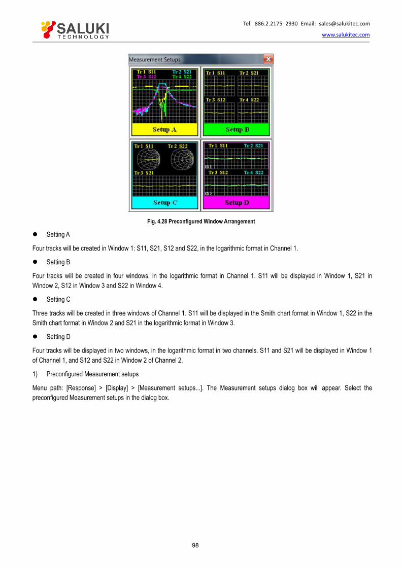
Tel: 886.2.2175 2930 Email: [email protected]
www.salukitec.com
98
Fig. 4.28 Preconfigured Window Arrangement
Setting A
Four tracks will be created in Window 1: S11, S21, S12 and S22, in the logarithmic format in Channel 1.
Setting B
Four tracks will be created in four windows, in the logarithmic format in Channel 1. S11 will be displayed in Window 1, S21 inWindow 2, S12 in Window 3 and S22 in Window 4.
Setting C
Three tracks will be created in three windows of Channel 1. S11 will be displayed in the Smith chart format in Window 1, S22 in theSmith chart format in Window 2 and S21 in the logarithmic format in Window 3.
Setting D
Four tracks will be displayed in two windows, in the logarithmic format in two channels. S11 and S21 will be displayed in Window 1of Channel 1, and S12 and S22 in Window 2 of Channel 2.
1) Preconfigured Measurement setups
Menu path: [Response] > [Display] > [Measurement setups...]. The Measurement setups dialog box will appear. Select thepreconfigured Measurement setups in the dialog box.

Tel: 886.2.2175 2930 Email: [email protected]
www.salukitec.com
99
Fig. 4.29 Pre-configured Measurement setups
2) Window arrangement
a) Several methods of window adjustment are provided in the analyzer.
Use the mouse to move and adjust the window.
Arrange the windows of the analyzer by the [Tile], [Cascade], [Maximize] and [Minimize] items of the
window menu.
Arrange the windows by the [One-window], [Two-window], [Three-window] and [Four-window] items of the display menu.
Use the [Minimize], [Maximize/reduce down] and [Close] button in the top right corner of the window to adjust or hide thewindow.
b) The display menu of the analyzer provides four kinds of window arrangement. The existing tracks are distributed into differentwindows according to a certain algorithm.
One-window arrangement
All tracks are displayed in one window in a cascading manner.
Two-window arrangement
All tracks are displayed in two windows which are vertically overlapped.
Three-window arrangement
All tracks are displayed in three windows. Two of the three windows are arranged in the upper part, and the other in the lower part.
Four-window arrangement
All tracks are displayed in four windows which respectively cover one fourth of the screen.
c) Setting of window arrangement
Menu path: [Response] > [Display]. The display sub-menu will pop up. Select the window arrangement mode in the displaysub-menu.
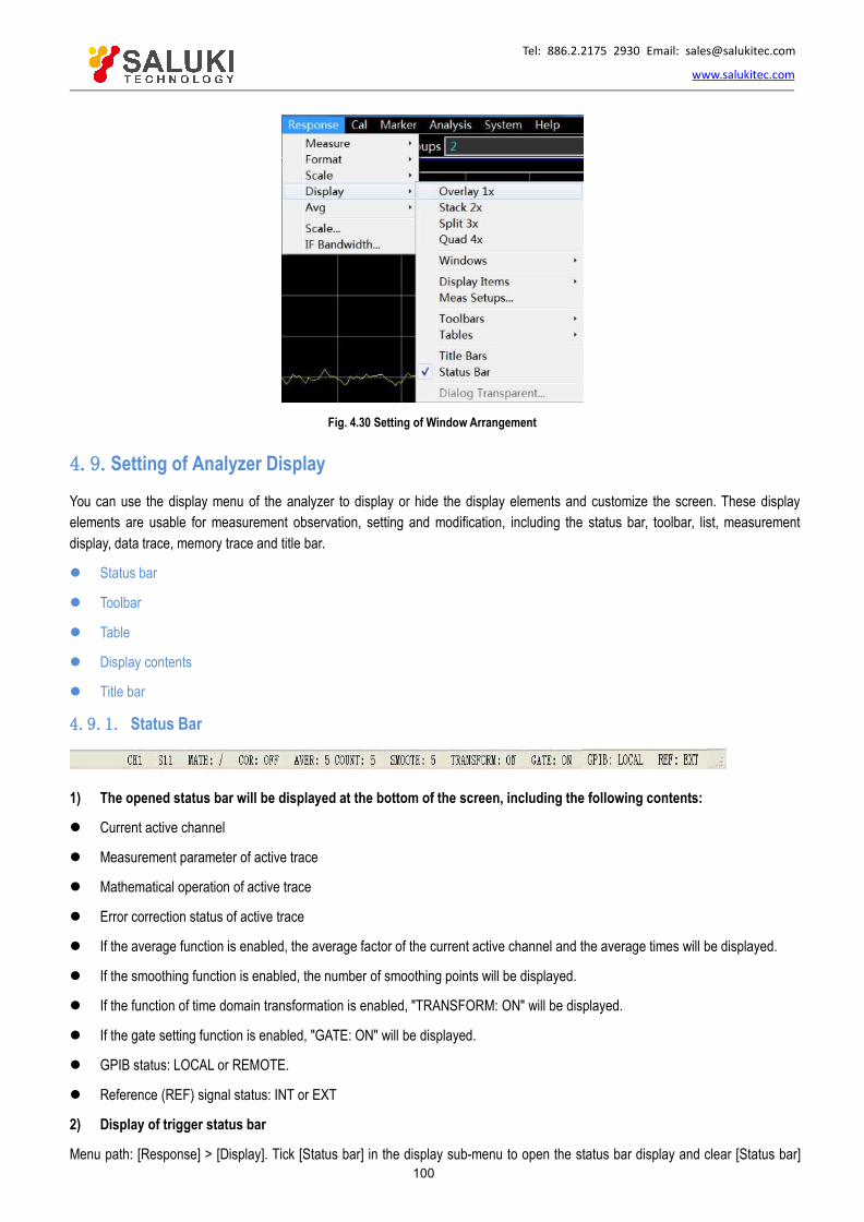
Tel: 886.2.2175 2930 Email: [email protected]
www.salukitec.com
100
Fig. 4.30 Setting of Window Arrangement
4.9.Setting of Analyzer Display
You can use the display menu of the analyzer to display or hide the display elements and customize the screen. These displayelements are usable for measurement observation, setting and modification, including the status bar, toolbar, list, measurementdisplay, data trace, memory trace and title bar.
Status bar
Toolbar
Table
Display contents
Title bar
4.9.1. Status Bar
1) The opened status bar will be displayed at the bottom of the screen, including the following contents:
Current active channel
Measurement parameter of active trace
Mathematical operation of active trace
Error correction status of active trace
If the average function is enabled, the average factor of the current active channel and the average times will be displayed.
If the smoothing function is enabled, the number of smoothing points will be displayed.
If the function of time domain transformation is enabled, "TRANSFORM: ON" will be displayed.
If the gate setting function is enabled, "GATE: ON" will be displayed.
GPIB status: LOCAL or REMOTE.
Reference (REF) signal status: INT or EXT
2) Display of trigger status bar
Menu path: [Response] > [Display]. Tick [Status bar] in the display sub-menu to open the status bar display and clear [Status bar]
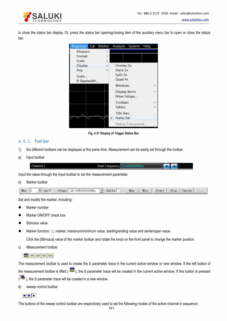
Tel: 886.2.2175 2930 Email: [email protected]
www.salukitec.com
101
to close the status bar display. Or, press the status bar opening/closing item of the auxiliary menu bar to open or close the statusbar.
Fig. 4.31 Display of Trigger Status Bar
4.9.2. Tool bar
1) Six different toolbars can be displayed at the same time. Measurement can be easily set through the toolbar.
a) Input toolbar
Input the value through the input toolbar to set the measurement parameter.
b) Marker toolbar
Set and modify the marker, including:
Marker number
Marker ON/OFF check box
Stimulus value
Marker function: marker, maximum/minimum value, starting/ending value and center/span value.
Click the [Stimulus] value of the marker toolbar and rotate the knob on the front panel to change the marker position.
c) Measurement toolbar
The measurement toolbar is used to create the S parameter trace in the current active window or new window. If the left button of
the measurement toolbar is lifted ( ), the S parameter trace will be created in the current active window. If this button is pressed
( ), the S parameter trace will be created in a new window.
d) sweep control toolbar
The buttons of the sweep control toolbar are respectively used to set the following modes of the active channel in sequence:
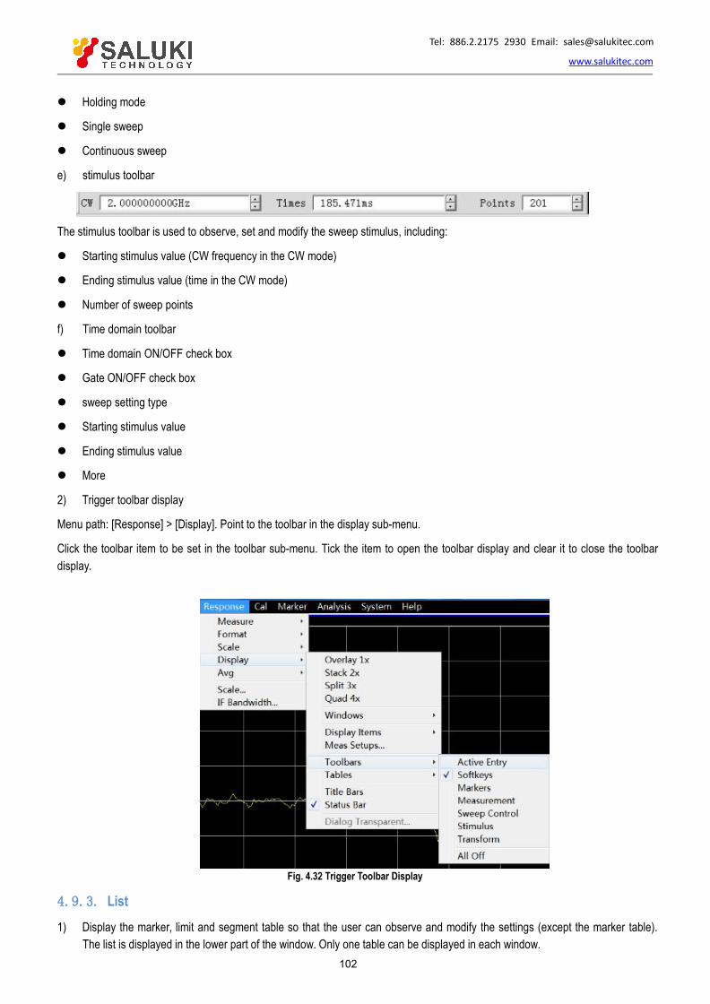
Tel: 886.2.2175 2930 Email: [email protected]
www.salukitec.com
102
Holding mode
Single sweep
Continuous sweep
e) stimulus toolbar
The stimulus toolbar is used to observe, set and modify the sweep stimulus, including:
Starting stimulus value (CW frequency in the CW mode)
Ending stimulus value (time in the CW mode)
Number of sweep points
f) Time domain toolbar
Time domain ON/OFF check box
Gate ON/OFF check box
sweep setting type
Starting stimulus value
Ending stimulus value
More
2) Trigger toolbar display
Menu path: [Response] > [Display]. Point to the toolbar in the display sub-menu.
Click the toolbar item to be set in the toolbar sub-menu. Tick the item to open the toolbar display and clear it to close the toolbardisplay.
Fig. 4.32 Trigger Toolbar Display
4.9.3. List
1) Display the marker, limit and segment table so that the user can observe and modify the settings (except the marker table).The list is displayed in the lower part of the window. Only one table can be displayed in each window.

Tel: 886.2.2175 2930 Email: [email protected]
www.salukitec.com
103
a) Marker table
Fig. 4.33 Marker Table
The marker table is used to display the marker parameters,including:
Marker number
Reference marker (for relative measurement)
Stimulus value
Response value
b) Limit table
Fig. 4.34 Limit Table
The limit table is used to display, set and modify the limit test parameters, including:
Type (minimum, maximum or closed)
Starting and ending stimulus value
Starting and ending response value
c) Segment table
Fig. 4.35 Segment Table
The segment table is used to display, set and modify the segment sweep parameters, including:
Status (ON/OFF)
Starting and ending stimulus value
Number of sweep points
Power level (separately set for each segment)
Intermediate frequency bandwidth (separately set for each segment)
Sweep time (separately set for each segment)
2) Triggering of table display
Menu path: [Response] > [Display]. Point to the [Table] in the display sub-menu.
Click the table to be triggered in the sub-menu. Tick this item to display the table and clear it to hide the table.
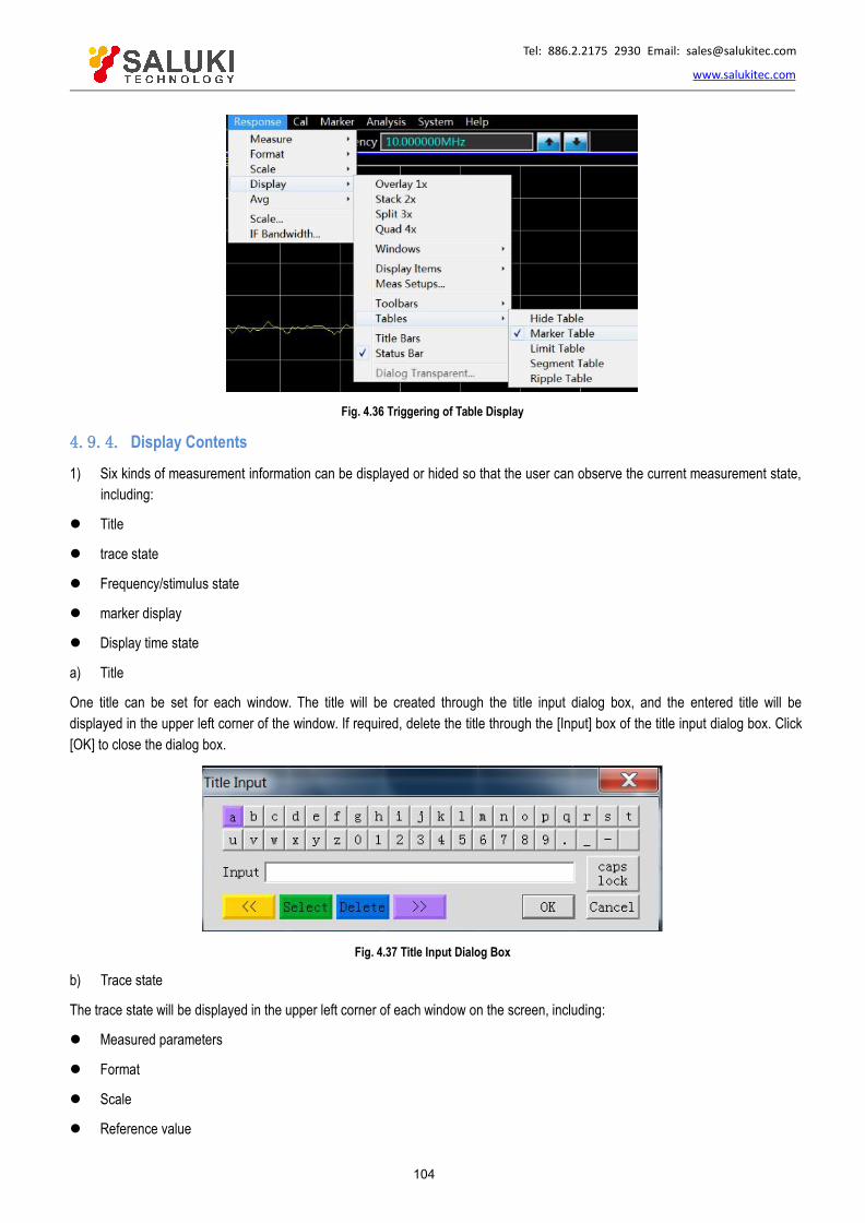
Tel: 886.2.2175 2930 Email: [email protected]
www.salukitec.com
104
Fig. 4.36 Triggering of Table Display
4.9.4. Display Contents
1) Six kinds of measurement information can be displayed or hided so that the user can observe the current measurement state,including:
Title
trace state
Frequency/stimulus state
marker display
Display time state
a) Title
One title can be set for each window. The title will be created through the title input dialog box, and the entered title will bedisplayed in the upper left corner of the window. If required, delete the title through the [Input] box of the title input dialog box. Click[OK] to close the dialog box.
Fig. 4.37 Title Input Dialog Box
b) Trace state
The trace state will be displayed in the upper left corner of each window on the screen, including:
Measured parameters
Format
Scale
Reference value
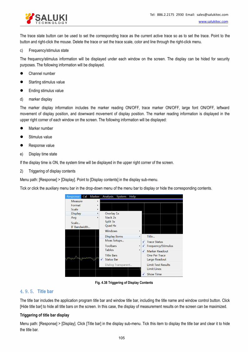
Tel: 886.2.2175 2930 Email: [email protected]
www.salukitec.com
105
The trace state button can be used to set the corresponding trace as the current active trace so as to set the trace. Point to thebutton and right-click the mouse. Delete the trace or set the trace scale, color and line through the right-click menu.
c) Frequency/stimulus state
The frequency/stimulus information will be displayed under each window on the screen. The display can be hided for securitypurposes. The following information will be displayed.
Channel number
Starting stimulus value
Ending stimulus value
d) marker display
The marker display information includes the marker reading ON/OFF, trace marker ON/OFF, large font ON/OFF, leftwardmovement of display position, and downward movement of display position. The marker reading information is displayed in theupper right corner of each window on the screen. The following information will be displayed:
Marker number
Stimulus value
Response value
e) Display time state
If the display time is ON, the system time will be displayed in the upper right corner of the screen.
2) Triggering of display contents
Menu path: [Response] > [Display]. Point to [Display contents] in the display sub-menu.
Tick or click the auxiliary menu bar in the drop-down menu of the menu bar to display or hide the corresponding contents.
Fig. 4.38 Triggering of Display Contents
4.9.5. Title barThe title bar includes the application program title bar and window title bar, including the title name and window control button. Click[Hide title bar] to hide all title bars on the screen. In this case, the display of measurement results on the screen can be maximized.
Triggering of title bar display
Menu path: [Response] > [Display]. Click [Title bar] in the display sub-menu. Tick this item to display the title bar and clear it to hidethe title bar.

Tel: 886.2.2175 2930 Email: [email protected]
www.salukitec.com
106
5. MenuThe menu is used to operate and set the vector network analyzer. S3602 series vector network analyzers are configured with a complexmenu system and setting dialog boxes under the menus at all levels. Be familiar with the menu system of the network analyzer tofacilitate operation. The menu system of S3602 series vector network analyzers is divided into the main menu, primary menu, secondarymenu, etc. The analyzer can be directly and partially set and operated through the menus at all levels. The setting and input dialog boxesunder the menus at various levels should be opened for some settings and operations.
Menu structure
Menu description
5.1.Menu structure
The menus at various levels are as follows:
File
Trace
Channel
Stimulus
Response
Calibration
Marker
Analysis
System
Help
5.1.1. File

Tel: 886.2.2175 2930 Email: [email protected]
www.salukitec.com
107
Fig. 5.1 File Menu
Note: Press the menu with an ellipsis (...) to open the corresponding dialog box, the same below.
5.1.2. Trace
Fig. 5.2 trace Menu
5.1.3. Channel
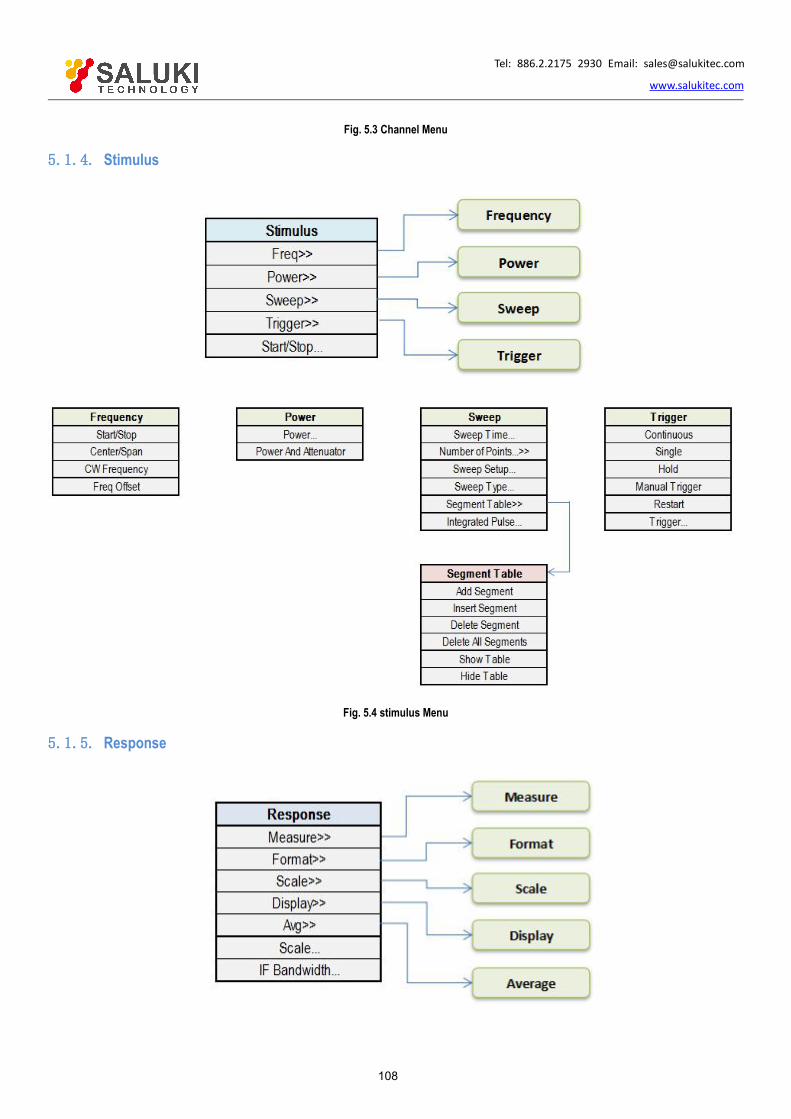
Tel: 886.2.2175 2930 Email: [email protected]
www.salukitec.com
108
Fig. 5.3 Channel Menu
5.1.4. Stimulus
Fig. 5.4 stimulus Menu
5.1.5. Response

Tel: 886.2.2175 2930 Email: [email protected]
www.salukitec.com
110
Fig. 5.5 Response Menu
5.1.6. Calibration
Fig. 5.6 Calibration Menu
5.1.7. Marker

Tel: 886.2.2175 2930 Email: [email protected]
www.salukitec.com
111
Fig. 5.7 Marker Menu
5.1.8. Analysis
Fig. 5.8 Analysis Menu
5.1.9. System

Tel: 886.2.2175 2930 Email: [email protected]
www.salukitec.com
112
Fig. 5.9 System menu
Fig. 5.10 Help Menu
1) Main menu
S3602 series vector network analyzers are configured with 10 main menus.
File: used to save, call and print test data, minimize the window and exit the program.
trace: used for relevant operations of tracks.
Channel: used for relevant operations of channels.
stimulus used for relevant setting of the stimulus signal.
Response: used for signal reception and measurement display setting.
Calibration: used for analyzer calibration and calibration setting.
marker: used for relevant operations of the marker system.
Analysis: used for analysis and statistics of test results and relevant setting of the time domain function.
System: used for relevant configuration setting, macro setting, pulse function setting, language setting, resetting and other settingsof the analyzer.
Help: used to call the user manual, program control manual and technical support, and view the error log and software versioninformation.
2) Sub-menu
The sub-menu of the main menu is the primary menu, the sub-menu of the primary menu is the secondary menu, and so on. In principle,

Tel: 886.2.2175 2930 Email: [email protected]
www.salukitec.com
113
the menu of higher level should be opened before opening the menu of lower level. For convenience, the commonly used secondarymenus are displayed in parallel to the menus of higher level.
3) Menu opening
Menus at various levels can be opened in the following three methods.
By the menu bar: click the main menu, and the primary menu will appear. Click the corresponding menu, and the menu of lowerlevel or corresponding dialog box will appear.
By keys of the front panel: press the main menu key in the functional key zone of the front panel, and the auxiliary menu bar willpop up, displaying the primary menu. Click the corresponding menu in the auxiliary menu bar, and the menu of lower level orcorresponding dialog box will appear.
For convenience, the shortcut menu bar is set on the right side of the auxiliary menu bar, including the commonly used menus.Drag the shortcut bar push-pull button on the left side of the auxiliary menu bar to display and hide the shortcut menu bar andauxiliary menu bar.
In order to facilitate introduction, the screenshots used in the manual are for menu opening by the menu bar.
5.2.Description of menu
This section introduces the details of the functions, parameters, etc. of menu items.
File
Trace
Channel
Stimulus
Response
Calibration
Marker
Analysis
System
Help
5.2.1. File
Press the [File] key on the front panel or the menu item [File] on the user interface. The file-related menu will pop up, including [Save>>],[Call>>] and [Print>>]. The specific description of menu items is as follows.
5.2.1.1. Save
This menu is used to save data. Click it to enter the menu of lower level. The specific menu includes:

Tel: 886.2.2175 2930 Email: [email protected]
www.salukitec.com
114
Table 5.2 Save
Save
Save As...
Define Data Saves…
1) Save
Function description:
Save user settings and calibration information in the data (*.CST) file.
The current user settings and calibration information will be saved in the latest user data file. If this item is clicked, the [Whether to coverprevious data] dialog box will pop up. Click "Yes" to cover previous data and save current data; and click "No" to abandon saving.
Parameter description:
None
2) Save as…
Function description:
Save the data file required by the user.
The data required by the user will be saved in different types of files. The user can set the file name. File types include: state andcalibration file (*.CST), state file (*.STA), calibration file, (*CAL), data file (*.DAT, *.CTI and *.S1P), bitmap file (*.BMP), etc.
Parameter description:
None
3) Define Data Saves…
Function description:
Save the file required by the user.
The parameters required by the user will be saved in different types of files. The user can set the file name. File types include the data file(*.DAT, *.CTI, *.S1P and *.S2P) and list file (*.PRN).
Parameter description:
None
5.2.1.2. Recall...
This menu is used to call the saved data. Click it to enter the menu of lower level. The specific menu includes:
Table 5.3 Call
Menu
Call

Tel: 886.2.2175 2930 Email: [email protected]
www.salukitec.com
115
1) Recall
Function description:
Call the saved state file or calibration file.
If this item is clicked, a state file or calibration file will be called. File types includes the state and calibration file (*.CST), state file (*.STA),calibration file (*CAL) and data file (*.DAT, *.CTI and *.S1P).
Parameter description:
None
5.2.1.3. Print>>
This menu is used to print data. Click it to enter the menu of lower level. The specific menu includes:
Table 5.4 Print
Print into file
Page Setup
1) Print
Function description:
Click this menu to enter the printer setting page.
Set the printer options, paper and direction according to the prompts.
Parameter description:
None
2) Print into file Function description:
Click this menu to save the test curve as a figure.
The test curve can be saved in the figure (*.BMP and *.JPJ) form according to the prompts.
Parameter description:
None
3) Page setting Function description:
Click this menu to enter the page setting interface.
The window information and other information can be set on this page. Window information includes: “Print active window", “Print allwindows" and “Print one window on each page". Other information includes: printing of the segment table, limit table, marker table,channel state and time. The user can print the corresponding page information according to the needs.
Parameter description:
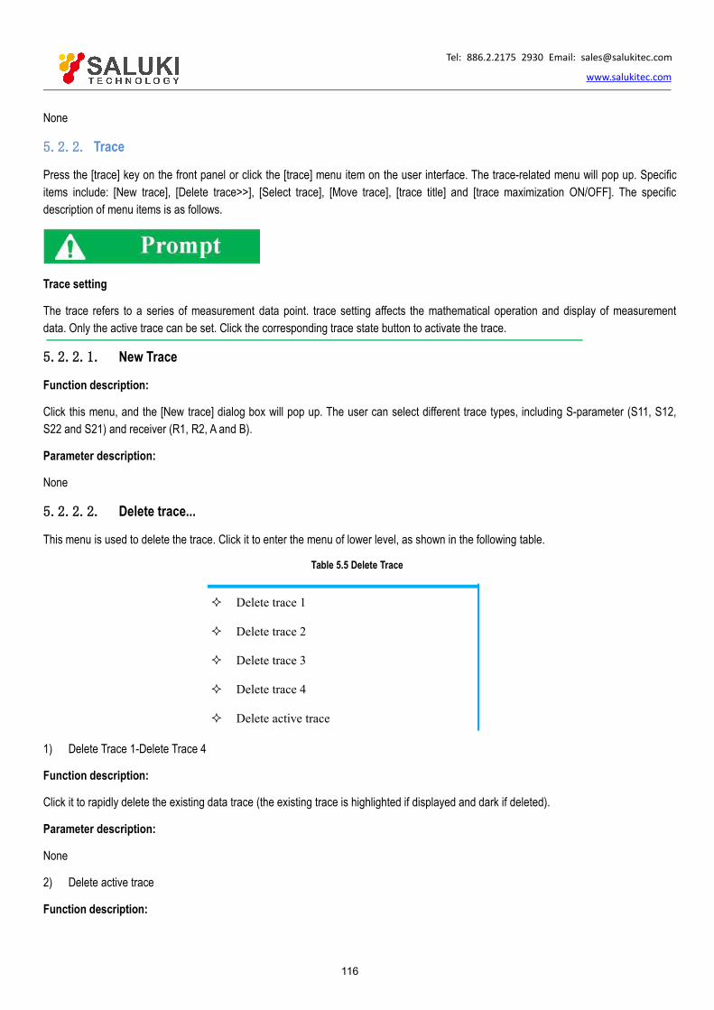
Tel: 886.2.2175 2930 Email: [email protected]
www.salukitec.com
116
None
5.2.2. Trace
Press the [trace] key on the front panel or click the [trace] menu item on the user interface. The trace-related menu will pop up. Specificitems include: [New trace], [Delete trace>>], [Select trace], [Move trace], [trace title] and [trace maximization ON/OFF]. The specificdescription of menu items is as follows.
Trace setting
The trace refers to a series of measurement data point. trace setting affects the mathematical operation and display of measurementdata. Only the active trace can be set. Click the corresponding trace state button to activate the trace.
5.2.2.1. New Trace
Function description:
Click this menu, and the [New trace] dialog box will pop up. The user can select different trace types, including S-parameter (S11, S12,S22 and S21) and receiver (R1, R2, A and B).
Parameter description:
None
5.2.2.2. Delete trace...
This menu is used to delete the trace. Click it to enter the menu of lower level, as shown in the following table.
Table 5.5 Delete Trace
Delete trace 1
Delete trace 2
Delete trace 3
Delete trace 4
Delete active trace
1) Delete Trace 1-Delete Trace 4
Function description:
Click it to rapidly delete the existing data trace (the existing trace is highlighted if displayed and dark if deleted).
Parameter description:
None
2) Delete active trace
Function description:

Tel: 886.2.2175 2930 Email: [email protected]
www.salukitec.com
117
Click this menu to delete the current active trace (click once to delete one active trace, until all active tracks are deleted).
Parameter description:
None
5.2.2.3. Move trace
Function description:
Click this menu, and the trace movement list will pop up, showing the existing windows. The user can move the current active trace intoany window (if [New window] is selected, a new window will be created). Click [Apply] to move the trace and continue the aboveoperation. Click [OK] to exit the program.
Parameter description:
None
5.2.2.4. Trace title
Function description:
Click this menu to change the default name of the current active curve. Enter the curve title, select the [Enable] check box and click [OK].Thus the trace title is changed.
Parameter description:
None
5.2.2.5. Trace max
Function description:
Click this menu to maximize the current active trace and hide other traces..
Parameter description:
OFF [OFF|ON].
5.2.3. Channel
Press the [Channel] key on the front panel or the [Channel] menu item on the user interface, and the channel-related menu will pop up forsetting of channel parameters. Specific items include: [Open channel], [Close channel], [Select channel], [Copy channel] and [Hardwaresetting]. The specific description of menu items is as follows.
Channel and Trace
The channel includes the trace. The analyzer supports 64 channels in total. Tracks in one channel are subject to the same channelsettings. Only the settings of the active channel can be changed. Once the trace in the channel is activated, the channel will also beactivated.
5.2.3.1. Open channel
Function description:

Tel: 886.2.2175 2930 Email: [email protected]
www.salukitec.com
118
Click this menu, and the [Open channel] list will pop up, showing the closed channels. The user can select the channel to be opened (if[New window] is selected, a new window will be created). Click [Apply] to open the channel and continue the above operation. Click [OK]to exit the program.
Parameter description:
None
5.2.3.2. Close channel
Function description:
Click this menu, and the [Close channel] list will pop up, showing the open channels. The user can select one channel, click [Apply] toclose the channel and then click [OK] to exit the program.
Parameter description:
None
5.2.3.3. Select channel
Function description:
Click this menu, and the [Select channel] list will pop up, showing the existing channels. The user can select the channel to be activated,click [Apply] to select the channel and then click [OK] to exit the program.
Parameter description:
None
5.2.3.4. Copy channel
Function description:
Click this menu, and the [Copy channel] list will pop up. The user can select the target channel from the existing channels in thedrop-down menu of [Copy channel], click [Apply] to copy the channel and then click [OK] to exit the program.
Parameter description:
None
5.2.3.5. Hardware setting>>
This menu is used for hardware setting. Click it to enter the menu of lower level, as shown in the following table.
Table 5.6 Hardware Setting
Menu
Path configuration
Graphic configuration
1) Path configuration
Function description:
Click this menu to configure the corresponding RF path.

Tel: 886.2.2175 2930 Email: [email protected]
www.salukitec.com
119
Parameter description:
None
2) Graphic configuration
Function description:
Click this menu to configure the filter/high power mode of the source and the reference mixer switch.
Parameter description:
None
5.2.4. Stimulus
Press the [Stimulus] key on the front panel or the [Stimulus] menu item on the user interface, and then stimulus- related menu will pop upfor setting of stimulus parameters. Specific items include: [Frequency], [Power], [Sweep] and [Trigger]. The specific description of menuitems is as follows.
5.2.4.1. Freq>>
This menu is used to set the frequency. Click it to enter the menu of lower level. The specific menu includes:
Table 5.7 Frequency
Freq Start
Freq Stop
center frequency
Frequency span
Frequency offset
CW
Frequency unit
All the frequency parameters are in Hz. The digital input must be ended with four frequency units (GHz, MHz, kHz or Hz). When inputends, new frequency value is displayed in appropriate unit.
The ending frequency must not exceed the starting frequency.
The sweeper can only sweep upward under stepped sweep mode, so ending frequency must be not less than starting frequency. Ifstarting frequency is more than ending frequency, ending frequency is equal to starting frequency; if ending frequency is less thanstarting frequency, starting frequency is equal to ending frequency.
1) Starting frequency

Tel: 886.2.2175 2930 Email: [email protected]
www.salukitec.com
120
Function description:
Set the starting point of the sweep frequency.
Set and adjust the parameter by the mouse/keyboard or the knob, number keys and stepping keys on the front panel.
Parameter description:
10MHz [10MHz - 67GHz].
2) Frequency Stop
Function description:
Set the ending point of sweep frequency.
Set and adjust the parameter by the mouse/keyboard or the knob, number keys and stepping keys on the front panel.
Parameter description:
67GHz [10MHz - 67GHz].
3) Center frequency
Function description:
Set the center point of sweep frequency.
Set and adjust the parameter by the mouse/keyboard or the knob, number keys and stepping keys on the front panel.
Parameter description:
33.505GHz[10MHz - 67GHz].
4) Frequency span
Function description: Set the span of frequency.
Set and adjust the parameter by the mouse/keyboard or the knob, number keys and stepping keys on the front panel.
Parameter description:
67GHz [10MHz - 67GHz].
5) Frequency Offset
Function description:
Set the offset of frequency.
This menu is used for relevant settings of the frequency offset.
Parameter description:
None
6) CW
Function description:
Set the CW frequency.
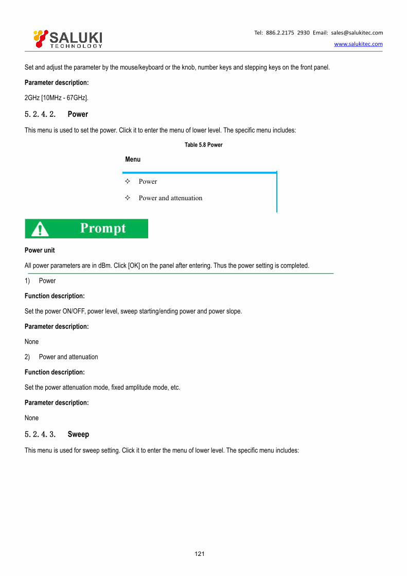
Tel: 886.2.2175 2930 Email: [email protected]
www.salukitec.com
121
Set and adjust the parameter by the mouse/keyboard or the knob, number keys and stepping keys on the front panel.
Parameter description:
2GHz [10MHz - 67GHz].
5.2.4.2. Power
This menu is used to set the power. Click it to enter the menu of lower level. The specific menu includes:
Table 5.8 Power
Menu
Power
Power and attenuation
Power unit
All power parameters are in dBm. Click [OK] on the panel after entering. Thus the power setting is completed.
1) Power
Function description:
Set the power ON/OFF, power level, sweep starting/ending power and power slope.
Parameter description:
None
2) Power and attenuation
Function description:
Set the power attenuation mode, fixed amplitude mode, etc.
Parameter description:
None
5.2.4.3. Sweep
This menu is used for sweep setting. Click it to enter the menu of lower level. The specific menu includes:

Tel: 886.2.2175 2930 Email: [email protected]
www.salukitec.com
122
Table 5.9 sweep: Segment Table
Menu Submenu
Sweep time Number of sweep points Sweep type Sweep setup Integrated Pulse Segment table>>
Segment table ON/OFFAdd segmentInsert segmentDelete segmentIndependent power level ON/OFFIndependent IF bandwidth ON/OFFIndependent sweep time ON/OFF
1) Sweep time
Function description:
Set the total time of sweep from the starting frequency to ending frequency.
Set and adjust the parameter by the mouse/keyboard or the knob, number keys and stepping keys on the front panel.
Reference note: (201points)
198ms [198ms-86400s].
2) Number of sweep points
Function description:
Set the total point number of sweep from the starting frequency to ending frequency.
Set and adjust the parameter by the mouse/keyboard or the knob, number keys and stepping keys on the front panel.
Parameter description:
201[1 - 32001].
3) Sweep type
Function description:
Set the sweep type.
Optional sweep types include: linear frequency, logarithmic frequency, power sweep, CW, segment sweep and phase sweep.
Parameter description:
None
4) Sweep setup
Function description:

Tel: 886.2.2175 2930 Email: [email protected]
www.salukitec.com
123
Set the sweep function.
The sweep functions include the step sweep, quick sweep, dwell time and sweep delay.
Parameter description:
None
5) Integrated Pulse
Function description:
Set the pulse measurement function.
Parameter description:
pulse duration: 33ns-60s
Pulse rising/falling time: 30ns
6) Segment table
This menu is used for relevant setting of the segment table. Click it to enter the menu of lower level. The specific menu includes:
Table 5.10 Segment Table
Menu
Add segment
Insert segment
Delete segment
Delete All Segments
Show Table
Hide Table
1) Add segment
Function description:
Add a new segment behind the existing segment.
Parameter description:
None
2) Insert segment
Function description:
Insert a new segment in front of the selected segment.
Parameter description:
None

Tel: 886.2.2175 2930 Email: [email protected]
www.salukitec.com
124
3) Delete segment
Function description:
Delete the selected segment.
Parameter description:
None
4) Delete all Segment
Function description:
Delete all segment
Parameter description:
None
5) Show Table
Function description:
Show segment table.
Parameter description:
None.
f) Hide table
Function description:
Hide Segment table
Parameter description:
None.
5.2.4.4. Trigger
This menu is used for trigger setting. Click it to enter the menu of lower level. The specific menu includes:

Tel: 886.2.2175 2930 Email: [email protected]
www.salukitec.com
125
Table 5.11 Trigger
Hold
Single
Continuous
Re-Start
Manual trigger
Trigger...
1) Hold
Function description:
If this menu is selected, the system will stop sweep and be kept at the current CW.
Parameter description:
None
2) Single
Function description:
If this menu is selected, the system will automatically enter the holding mode after sweep once.
Parameter description:
None
3) Continuous
Function description:
If this menu is selected, the system will restart sweep after sweep once.
Parameter description:
None
3) Restart
Function description:
If this menu is selected, the system will restart sweep from the starting frequency.
Parameter description:
None
4) Manual trigger
Function description:

Tel: 886.2.2175 2930 Email: [email protected]
www.salukitec.com
126
Set the trigger menu to light up this menu. If this menu is selected, manual triggering will be done once.
Parameter description:
None
5) Trigger...
Function description:
Select this menu to enter the trigger function setting interface.
Parameter description:
None
5.2.5. Response
Press the [Response] key on the front panel or the [Response] menu item on the user interface, and the response- related menu will popup. Specific items include: [Measurement], [Format], [Scale], [Display] and [Average]. The specific description of menu items is asfollows.
5.2.5.1. Measurement
This menu is used to set measurement. Click it to enter the menu of lower level. The specific menu includes:
Table 5.12 Measurement
Measurement S-parameter
Measurement balance parameter
Measuring class
Measuring receiver
1) Measurement S-parameter
Function description:
Select this menu to select the S-parameter.
Parameter description:
None
2) Measurement balance parameter
Function description:
Select this menu to select the balance parameter.
Parameter description:
None
3) Measuring class

Tel: 886.2.2175 2930 Email: [email protected]
www.salukitec.com
127
Function description:
Select this menu to enter the multi-functional measurement option setting interface, such as the mixer measurement.
Parameter description:
None
4) Measurement receiver
Function description:
Select this menu to select the receiver parameter, such as R1, R2, A, B, etc.
Parameter description:
None
5.2.5.2. Format
This menu is used to set measurement. Click it to enter the menu of lower level. The specific menu includes:
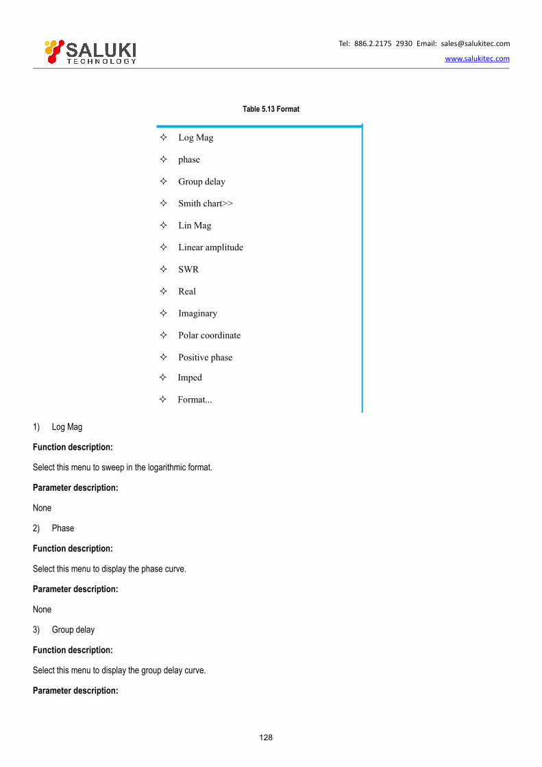
Tel: 886.2.2175 2930 Email: [email protected]
www.salukitec.com
128
Table 5.13 Format
Log Mag
phase
Group delay
Smith chart>>
Lin Mag
Linear amplitude
SWR
Real
Imaginary
Polar coordinate
Positive phase
Imped
Format...
1) Log Mag
Function description:
Select this menu to sweep in the logarithmic format.
Parameter description:
None
2) Phase
Function description:
Select this menu to display the phase curve.
Parameter description:
None
3) Group delay
Function description:
Select this menu to display the group delay curve.
Parameter description:

Tel: 886.2.2175 2930 Email: [email protected]
www.salukitec.com
129
None
4) Smith chart >>
Function description:
Select this menu to display the Smith chart curve.
Parameter description:
None
5) Lin Mag
Function description:
Select this menu to display the linear phase curve.
Parameter description:
None
6) Lin Mag
Function description:
Select this menu to display the linear amplitude curve.
Parameter description:
None
7) SWR
Function description:
Select this menu to display the standing wave ratio curve.
Parameter description:
None
8) Real
Function description:
Select this menu to display the real part curve.
Parameter description:
None
9) Imaginary
Function description:
Select this menu to display the imaginary part curve.
Parameter description:
None
Tel: 886.2.2175 2930 Email: [email protected]
www.salukitec.com
130
10) Polar coordinate
Function description:
Select this menu to display the polar coordinate curve.
Parameter description:
None
11) Positive phase
Function description:
Select this menu to display the positive phase curve.
Parameter description:
None
12) Imped
Function description:
Select this menu to display the impedance curve.
Parameter description:
None
13) Format
Function description:
If this menu is selected, the display format table will pop up. Multiple format curves can be selected.
Parameter description:
None
5.2.5.3. Scale
This menu is used to set the scale. Click it to enter the menu of lower level. The specific menu includes:

Tel: 886.2.2175 2930 Email: [email protected]
www.salukitec.com
131
Table 5.14 Format
Autoscale
Autoscale All
Scale..
Electrical delay
Phase offset
Mag Offset
Scale coupling
1) Automatic scale
Function description:
If this menu is selected, the vertical scale will be selected automatically so that the active trace can be better displayed in the vertical gridof the screen. The stimulus is not affected, and only the scale value and reference value are changed.
The appropriate scale factor will be selected so that data can be displayed in 80% of the screen. Select the center value of the trace onthe screen according to the reference value.
Parameter description:
None
2) Autoscale All
Function description:
If this menu is selected, the appropriate scale will be set for all tracks in the window so that the trace can be
better displayed in the vertical grids of the window.
Parameter description:
None
3) Scale
Function description:
Select this menu and enter the set scale value.
Set and adjust the parameter by the mouse/keyboard or the knob, number keys and stepping keys on the front panel.
Parameter description:
10dB[0.001dB-500dB].
4) Electrical delay

Tel: 886.2.2175 2930 Email: [email protected]
www.salukitec.com
132
Function description:
Select this menu to set the electrical delay.
Set and adjust the parameter by the mouse/keyboard or the knob, number keys and stepping keys on the front panel.
Parameter description:
0s[-1000s to 1000s].
5) Phase offset
Function description:
Select this menu to set the phase offset. Set and adjust the parameter by the mouse/keyboard or the knob, number keys and steppingkeys on the front panel.
Parameter description:
0° [-1000° to 1000°].
6) Mag Offset
Function description:
Select this menu to set the amplitude offset.
Set and adjust the parameter by the mouse/keyboard or the knob, number keys and stepping keys on the front panel.
Parameter description:
0dB[-1000dB - 1000dB]。
7) Scale coupling
Function description:
Select this menu to set scale coupling.
Parameter description:
None
5.2.5.4. Display
This menu is used to set the scale. Click it to enter the menu of lower level. The specific menu includes:
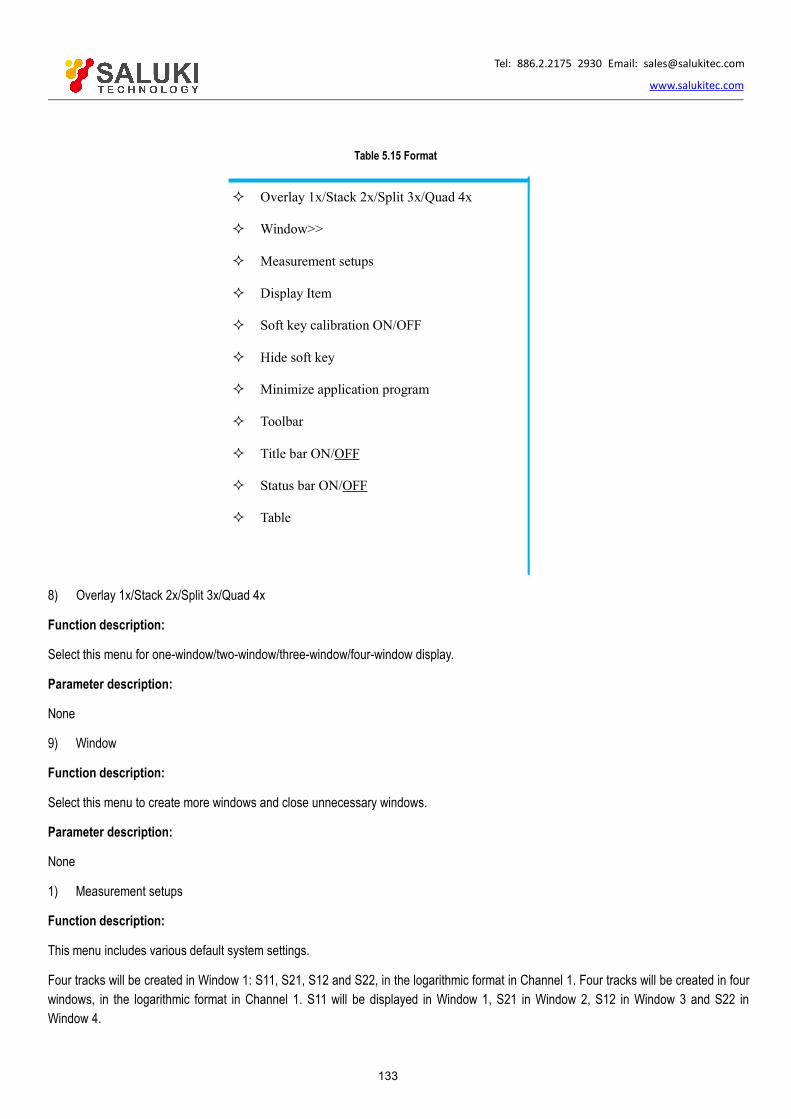
Tel: 886.2.2175 2930 Email: [email protected]
www.salukitec.com
133
Table 5.15 Format
Overlay 1x/Stack 2x/Split 3x/Quad 4x
Window>>
Measurement setups
Display Item
Soft key calibration ON/OFF
Hide soft key
Minimize application program
Toolbar
Title bar ON/OFF
Status bar ON/OFF
Table
8) Overlay 1x/Stack 2x/Split 3x/Quad 4x
Function description:
Select this menu for one-window/two-window/three-window/four-window display.
Parameter description:
None
9) Window
Function description:
Select this menu to create more windows and close unnecessary windows.
Parameter description:
None
1) Measurement setups
Function description:
This menu includes various default system settings.
Four tracks will be created in Window 1: S11, S21, S12 and S22, in the logarithmic format in Channel 1. Four tracks will be created in fourwindows, in the logarithmic format in Channel 1. S11 will be displayed in Window 1, S21 in Window 2, S12 in Window 3 and S22 inWindow 4.

Tel: 886.2.2175 2930 Email: [email protected]
www.salukitec.com
134
Three tracks will be created in three windows of Channel 1. S11 will be displayed in the Smith chart format in Window 1, S22 in the Smithchart format in Window 2 and S21 in the logarithmic format in Window 3.
Four tracks will be displayed in two windows, in the logarithmic format in two channels. S11 and S21 will be displayed in Window 1 ofChannel 1, and S12 and S22 in Window 2 of Channel 2.
Parameter description:
None
2) Display content
Function description:
Select this menu to control part of display contents, such as the title, trace state, frequency/stimulus state, marker display, display time,etc.
Parameter description:
None
3) Soft key calibration ON/OFF
Function description:
Select this menu to calibrate keys in the soft keyboard form to facilitate the user of old users.
Parameter description:
OFF [OFF|ON].
4) Hide soft key
Function description:
Select this menu to hide the soft keyboard on the right side of the display. The curve will be displayed in the whole screen.
Parameter description:
None
5) Minimize application program
Function description:
Select this menu to minimize the soft key in operation in the vector network analyzer.
Parameter description:
None
6) Tool bar
Function description:
Select this menu to control the toolbar display, such as the input toolbar, marker toolbar, measurement toolbar, sweep toolbar, stimulustoolbar and time domain toolbar.
Parameter description:

Tel: 886.2.2175 2930 Email: [email protected]
www.salukitec.com
135
None
7) Title bar ON/OFF
Function description:
Select this menu to display the title bar.
Parameter description:
None
8) Status bar ON/OFF
Function description:
Select this menu to display the status bar.
Parameter description:
None
9) Table
Function description:
Select this menu to display the marker table, limit table and segment table.
Parameter description:
None
5.2.5.5. Average
This menu is used to set the scale. Click it to enter the menu of lower level. The specific menu includes:
Table 5.16 Average
Restart average
Averaging factor
Average ON/OFF
Smoothing
IF bandwidth
1) Restart average
Function description:
Select this menu for a group of new average sweep.
Parameter description:
None
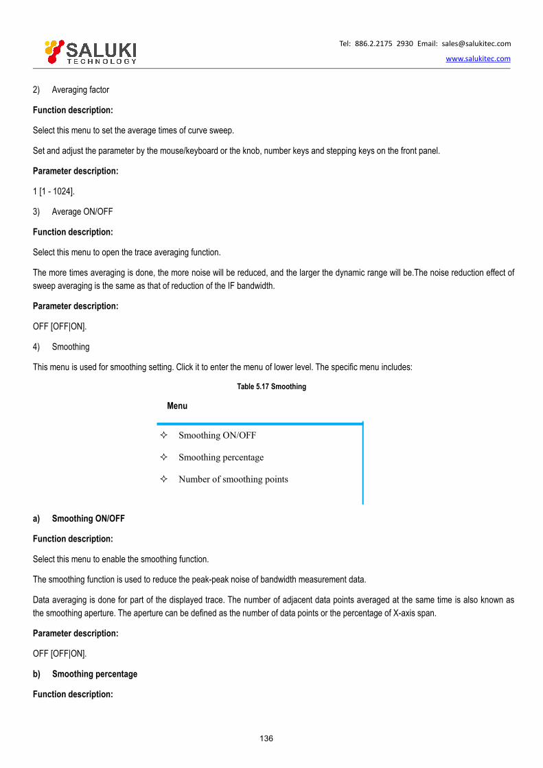
Tel: 886.2.2175 2930 Email: [email protected]
www.salukitec.com
136
2) Averaging factor
Function description:
Select this menu to set the average times of curve sweep.
Set and adjust the parameter by the mouse/keyboard or the knob, number keys and stepping keys on the front panel.
Parameter description:
1 [1 - 1024].
3) Average ON/OFF
Function description:
Select this menu to open the trace averaging function.
The more times averaging is done, the more noise will be reduced, and the larger the dynamic range will be.The noise reduction effect ofsweep averaging is the same as that of reduction of the IF bandwidth.
Parameter description:
OFF [OFF|ON].
4) Smoothing
This menu is used for smoothing setting. Click it to enter the menu of lower level. The specific menu includes:
Table 5.17 Smoothing
Menu
Smoothing ON/OFF
Smoothing percentage
Number of smoothing points
a) Smoothing ON/OFF
Function description:
Select this menu to enable the smoothing function.
The smoothing function is used to reduce the peak-peak noise of bandwidth measurement data.
Data averaging is done for part of the displayed trace. The number of adjacent data points averaged at the same time is also known asthe smoothing aperture. The aperture can be defined as the number of data points or the percentage of X-axis span.
Parameter description:
OFF [OFF|ON].
b) Smoothing percentage
Function description:

Tel: 886.2.2175 2930 Email: [email protected]
www.salukitec.com
137
Select this menu to set the smoothing percentage.
Set and adjust the parameter by the mouse/keyboard or the knob, number keys and stepping keys on the front panel.
Parameter description:
0 [0-25%].
c) Number of smoothing points
Function description:
This menu is used to set the number of smoothing points.
Set and adjust the parameter by the mouse/keyboard or the knob, number keys and stepping keys on the front panel.
Parameter description:
0 [0 - N (total point number)*25%].
5) Intermediate frequency bandwidth
Function description:
Select this menu to set the IF bandwidth.
Set and adjust the parameter by the mouse/keyboard or the knob, number keys and stepping keys on the front panel.
Parameter description:
1kHz [1Hz - 5MHz].
5.2.6. Calibration
Press the [Calibration] key on the front panel or the [Calibration] menu item on the user interface. The calibration- related menu will popup. Specific items include: [Calibration], [Correction ON/OFF], [Interpolation ON/OFF], [Port extension], [Fixture>>], [Edit calibration kit],[Attribute] and [Power calibration]. The specific description of menu items is as follows.
5.2.6.1. Calibration
Function description:
Select this menu to enter the calibration interface, including three calibration types: guided calibration, non-guided calibration andelectronic calibration. Select the appropriate calibration method according to the measurement type and accuracy requirements. Seedetails in 6.3 Calibration Guide.
Parameter description:
None
5.2.6.2. Correction ON/OFF
Function description:
Select this menu to enable the correction function and add calibration data.
Parameter description:
OFF [OFF|ON].

Tel: 886.2.2175 2930 Email: [email protected]
www.salukitec.com
138
5.2.6.3. Interpolation ON/OFF
Function description:
Select this menu to enable the interpolation function.
Parameter description:
OFF [OFF|ON].
5.2.6.4. Port Extension
Function description:
Select this menu to move the measurement reference plane in an electrical manner. Thus, other kinds of calibration can be avoided.
Add a cable after calibration. The port extension function is used to “tell" the length of the cable added to the specific port of the analyzer.In case of failure of direct calibration, the delay (phase shift) caused by the clamp can be compensated by port extension. For the methodof port extension setting, refer to the section of port extension in 5.5 Improvement of Phase Measurement Accuracy.
Parameter description:
None
5.2.6.5. Fixture>>
This menu is used to set the fixture function. Click it to enter the menu of lower level. The specific menu includes:
Table 5.18 Fixture
Menu
Fixture ON/OFF
Port Matching...
2-port de-embedding
Port impedance conversion...
Four-port fixture de-embedding/embedding
1) Fixture ON/OFF
Function description:
Select this menu to enable the fixture simulator function. The functions of the fixture simulator are effective only in this mode.
Parameter description:
OFF [OFF|ON].
2) Port Matching...
Function description:
Select this menu to enable the Port Matching... function. For setting of Port Matching..., refer to “7.9.3 Port Matching...” in “7.9 FixtureCompensation Calibration”.
Tel: 886.2.2175 2930 Email: [email protected]
www.salukitec.com
139
Parameter description:
None
3) 2-port de-embedding
Function description:
Select this menu to enable the 2-port de-embedding function. For setting of 2-port de-embedding, refer to “7.9.4 2-port de-embedding” in“7.9 Fixture Compensation Calibration”.
Parameter description:
None
4) Port impedance conversion...
Function description:
Select this menu to enable the port impedance conversion... function. For setting of port impedance conversion..., refer to “7.9.5 Portimpedance conversion...” in “7.9 Fixture Compensation Calibration”.
Parameter description:
None
5) Four-port fixture de-embedding/embedding
Function description:
Select this menu to enable the four-port fixture de-embedding/embedding function. For setting of port impedance conversion..., refer to“7.9.6 Four-port fixture de-embedding/embedding” in “7.9 Fixture Compensation Calibration”.
Parameter description:
None
5.2.6.6. Editing of Calibration Kit
Function description:
Select this menu to define and edit the calibration kit information. For calibration kit editing, refer to “7.6.3 Edit calibration kit” in “7.6Definition of Calibration Kit Editing”.
Parameter description:
None
5.2.6.7. Attribute
Function description:
This menu is effective after calibration of the instrument. Select this menu to display the current calibration attribute, such as the channel,calibration time, calibration type, frequency, number of sweep points, sweep time, port power, sweep type, etc.
Parameter description:
None

Tel: 886.2.2175 2930 Email: [email protected]
www.salukitec.com
140
5.2.6.8. Power Calibration
Function description:
Select this menu to set the source power, receiver calibration, etc. For power calibration setting, refer to “Port power calibration” in “6.3Calibration of scale mixer measurement”.
Parameter description:
None
5.2.7. Marker
Press the [Marker] key on the front panel or click the [Marker] menu item on the user interface. The Marker- related menu will pop up.Specific items include: [Marker], [Marker function], [Marker search], [Marker attribute] and [Marker display]. The specific description ofmenu items is as follows.
5.2.7.1. Marker
This menu is used to set the marker. Click it to enter the menu of lower level. The specific menu includes:
Table 5.19 Marker
Marker>>
Marker Function
More Marker
Close Marker
1) Marker 1/2/3>>
Function description:
Select this menu to enable the function of marker 1/2/3. Read the measurement data, search the value of specific type or change thestimulus setting.
Parameter description:
None
2) Marker Function
Function description:
Select this menu to enable the reference marker function for relative measurement.
Parameter description:
None
3) More Marker
Function description:
Select this menu to enter the “More Markers” page. The system is configured with marker 4, marker 5,marker 6, marker 7, marker 8 and
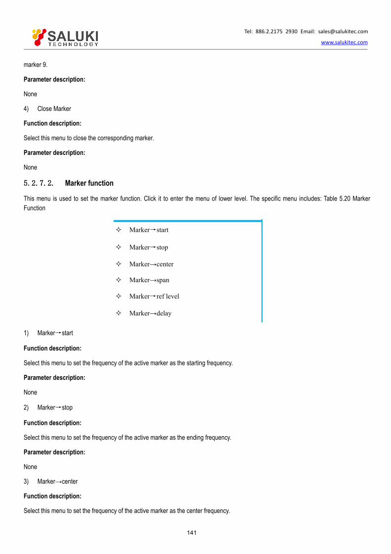
Tel: 886.2.2175 2930 Email: [email protected]
www.salukitec.com
141
marker 9.
Parameter description:
None
4) Close Marker
Function description:
Select this menu to close the corresponding marker.
Parameter description:
None
5.2.7.2. Marker function
This menu is used to set the marker function. Click it to enter the menu of lower level. The specific menu includes: Table 5.20 MarkerFunction
Marker→start
Marker→stop
Marker→center
Marker→span
Marker→ref level
Marker→delay
1) Marker→start
Function description:
Select this menu to set the frequency of the active marker as the starting frequency.
Parameter description:
None
2) Marker→stop
Function description:
Select this menu to set the frequency of the active marker as the ending frequency.
Parameter description:
None
3) Marker→center
Function description:
Select this menu to set the frequency of the active marker as the center frequency.
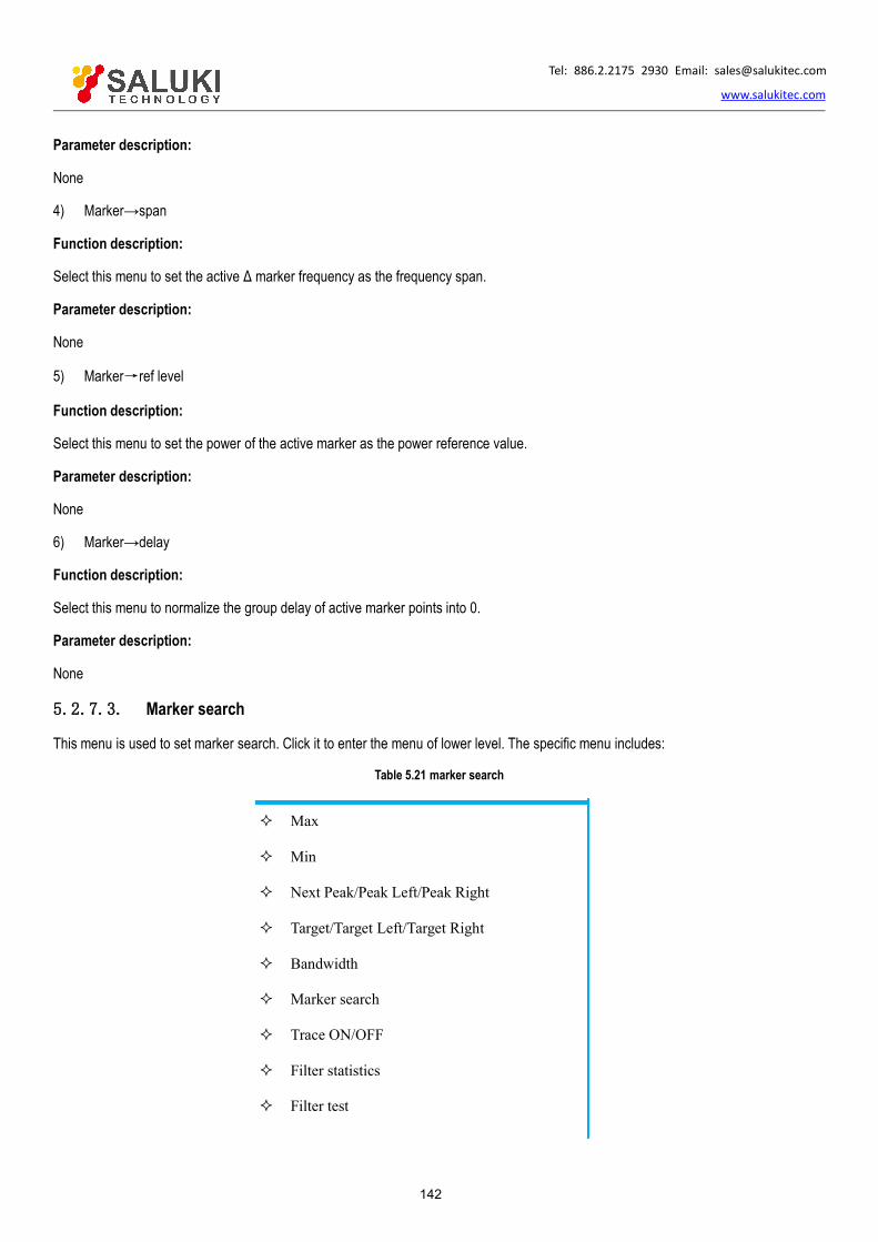
Tel: 886.2.2175 2930 Email: [email protected]
www.salukitec.com
142
Parameter description:
None
4) Marker→span
Function description:
Select this menu to set the active Δ marker frequency as the frequency span.
Parameter description:
None
5) Marker→ref level
Function description:
Select this menu to set the power of the active marker as the power reference value.
Parameter description:
None
6) Marker→delay
Function description:
Select this menu to normalize the group delay of active marker points into 0.
Parameter description:
None
5.2.7.3. Marker search
This menu is used to set marker search. Click it to enter the menu of lower level. The specific menu includes:
Table 5.21 marker search
Max
Min
Next Peak/Peak Left/Peak Right
Target/Target Left/Target Right
Bandwidth
Marker search
Trace ON/OFF
Filter statistics
Filter test

Tel: 886.2.2175 2930 Email: [email protected]
www.salukitec.com
143
1) Max
Function description:
Select this menu for marker search of the maximum measurement data point.
Parameter description:
None
2) Min
Function description:
Select this menu for marker search of the minimum measurement data point.
Parameter description:
None
3) Peak Value
This menu is used to set the peak search. Click it to enter the menu of lower level. The specific menu includes:
Table 5.22 Peak Value
Next peak value
Right peak value
Left peak value
Peak/valley type
Threshold
Offset
a) Next peak value
Function description:
Select this menu to search next peak value lower than the current marker amplitude value.
Parameter description:
None
b) Right peak value
Function description:
Select this menu to search next effective peak value on the right side of the marker position.
Parameter description:
None
c) Left peak value

Tel: 886.2.2175 2930 Email: [email protected]
www.salukitec.com
144
Function description:
Select this menu to search next effective peak value on the left side of the marker position.
Parameter description:
OFF [OFF|ON].
d) Peak/valley type
Function description:
Select this menu to select the peak type.
Parameter description:
Peak [Valley|Peak].
e) Threshold
Function description:
Select this menu to define the minimum peak value. The effective peak value must be more than the threshold. The valley values on bothsides may be less than the threshold.
Set and adjust the parameter by the mouse/keyboard or the knob, number keys and stepping keys on the front panel.
Parameter description:
-100dB [-500dB to 500dB].
f) Deviation
Function description:
Select this menu to define the minimum vertical distance between the peak value and valley value. The vertical distance between theeffective peak value and valley values on both sides must be more than the deviation.
Set and adjust the parameter by the mouse/keyboard or the knob, number keys and stepping keys on the front panel.
Parameter description:
3dB [-500dB - 500dB].
4) Target value
Function description:
Select this menu and enter the search target value. If this menu is clicked once, the marker will move to the first target value on the rightside of the current marker position. Continue the above operation to reach to the highest stimulus value. Then return to the minimumsearch target value of stimulus.
Set and adjust the parameter by the mouse/keyboard or the knob, number keys and stepping keys on the front panel.
Parameter description:
0dB [-500dB - 500dB].
5) Bandwidth search
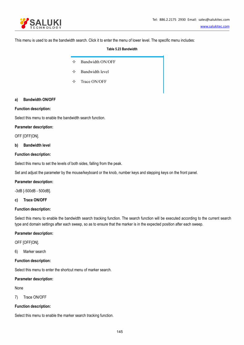
Tel: 886.2.2175 2930 Email: [email protected]
www.salukitec.com
145
This menu is used to as the bandwidth search. Click it to enter the menu of lower level. The specific menu includes:
Table 5.23 Bandwidth
Bandwidth ON/OFF
Bandwidth level
Trace ON/OFF
a) Bandwidth ON/OFF
Function description:
Select this menu to enable the bandwidth search function.
Parameter description:
OFF [OFF|ON].
b) Bandwidth level
Function description:
Select this menu to set the levels of both sides, falling from the peak.
Set and adjust the parameter by the mouse/keyboard or the knob, number keys and stepping keys on the front panel.
Parameter description:
-3dB [-500dB - 500dB].
c) Trace ON/OFF
Function description:
Select this menu to enable the bandwidth search tracking function. The search function will be executed according to the current searchtype and domain settings after each sweep, so as to ensure that the marker is in the expected position after each sweep.
Parameter description:
OFF [OFF|ON].
6) Marker search
Function description:
Select this menu to enter the shortcut menu of marker search.
Parameter description:
None
7) Trace ON/OFF
Function description:
Select this menu to enable the marker search tracking function.

Tel: 886.2.2175 2930 Email: [email protected]
www.salukitec.com
146
Parameter description:
OFF [OFF|ON].
8) Filter statistics ON/OFF
Function description:
Select this menu to enable the function of filter statistics.
Parameter description:
OFF [OFF|ON].
9) Filter test
This menu is used to set the filter test. Click it to enter the menu of lower level. The specific menu includes:
Table 5.24 Filter Test
Filter test ON/OFF
Bandwidth level
Frequency difference percentage
Trace ON/OFF
a) Filter test ON/OFF
Function description:
Select this menu to enable the filter test function.
Parameter description:
OFF [OFF|ON].
b) Bandwidth level
Function description:
Select this menu to set the filter bandwidth level.
Set and adjust the parameter by the mouse/keyboard or the knob, number keys and stepping keys on the front panel.
Parameter description:
-3dB [-500dB - 500dB].
c) Frequency difference percentage
Function description:
Select this menu to set the frequency difference percentage.
Set and adjust the parameter by the mouse/keyboard or the knob, number keys and stepping keys on the front panel.
Parameter description:

Tel: 886.2.2175 2930 Email: [email protected]
www.salukitec.com
147
10% [0% to 100%].
d) Trace ON/OFF
Function description:
Select this menu to enable the marker tracking function for the filter test.
Parameter description:
OFF [OFF|ON].
5.2.7.4. Marker attribute
This menu is used to set the marker attribute. Click it to enter the menu of lower level. The specific menu includes:
Table 5.25 Marker Attribute
Δmarker ON/OFF
Discrete ON/OFF
Type Normal/Fixed
Coupling ON/OFF
Advanced marker
1) Δ marker ON/OFF
Function description:
Select this menu to enable the Δ marker function.
Parameter description:
OFF [OFF|ON].
2) Discrete ON/OFF
Function description:
Select this menu to enable the discrete marker function. The marker will be moved to the discrete data point equivalent to the targetvalue.
Parameter description:
OFF [OFF|ON].
3) Type Normal/Fixed
Function description:
Select this menu to select the marker type.
Normal: the X-axis position of the standard marker is fixed, and the Y-axis position changes along with the amplitude of trace data. Themarker can be moved right and left on the X-axis by changing the stimulus value.
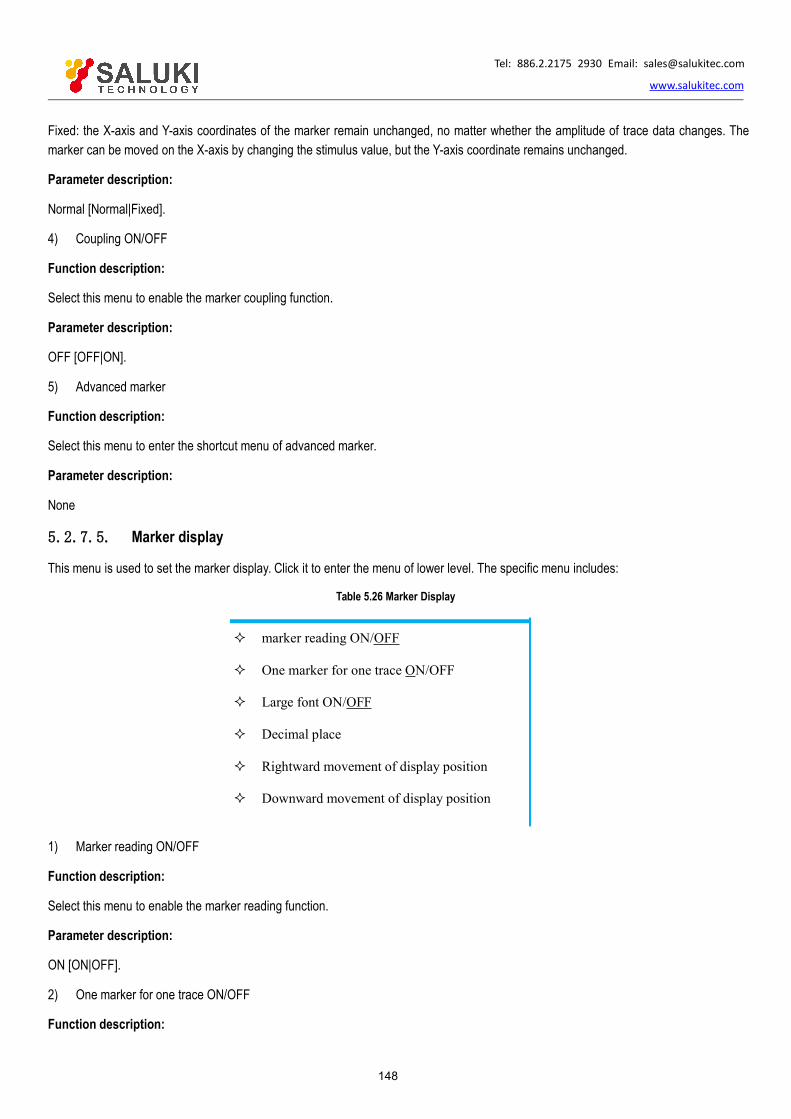
Tel: 886.2.2175 2930 Email: [email protected]
www.salukitec.com
148
Fixed: the X-axis and Y-axis coordinates of the marker remain unchanged, no matter whether the amplitude of trace data changes. Themarker can be moved on the X-axis by changing the stimulus value, but the Y-axis coordinate remains unchanged.
Parameter description:
Normal [Normal|Fixed].
4) Coupling ON/OFF
Function description:
Select this menu to enable the marker coupling function.
Parameter description:
OFF [OFF|ON].
5) Advanced marker
Function description:
Select this menu to enter the shortcut menu of advanced marker.
Parameter description:
None
5.2.7.5. Marker display
This menu is used to set the marker display. Click it to enter the menu of lower level. The specific menu includes:
Table 5.26 Marker Display
marker reading ON/OFF
One marker for one trace ON/OFF
Large font ON/OFF
Decimal place
Rightward movement of display position
Downward movement of display position
1) Marker reading ON/OFF
Function description:
Select this menu to enable the marker reading function.
Parameter description:
ON [ON|OFF].
2) One marker for one trace ON/OFF
Function description:

Tel: 886.2.2175 2930 Email: [email protected]
www.salukitec.com
149
Select this menu to enable the function of one marker for one trace.
Parameter description:
OFF [OFF|ON].
3) Large font ON/OFF
Function description:
Select this menu to enable the function of large font display of the marker.
Parameter description:
OFF [OFF|ON].
Decimal place
Function description:
Select this menu to set the number of decimal places of marker display.
Set and adjust the parameter by the mouse/keyboard or the knob, number keys and stepping keys on the front panel.
Parameter description:
2 [0 - 4].
4) Rightward movement of display position
Function description:
Select this menu to set the horizontal position of the marker.
Set and adjust the parameter by the mouse/keyboard or the knob, number keys and stepping keys on the front panel.
Parameter description:
80% [-200% to 200%].
5) Downward movement of display position
Function description:
Select this menu to set the vertical position of the marker.
Set and adjust the parameter by the mouse/keyboard or the knob, number keys and stepping keys on the front panel.
Parameter description:
80% [-200% to 200%].
5.2.8. Analysis
Press the [Analysis] key on the front panel or the [Analysis] menu item on the user interface. The analysis-related menu will pop up.Specific items include: [Save], [Test], [trace statistics], [Gate], [Window], [Time domain], [Structural return loss] and [Equation Editor]. Thespecific description of menu items is as follows.
5.2.8.1. Save
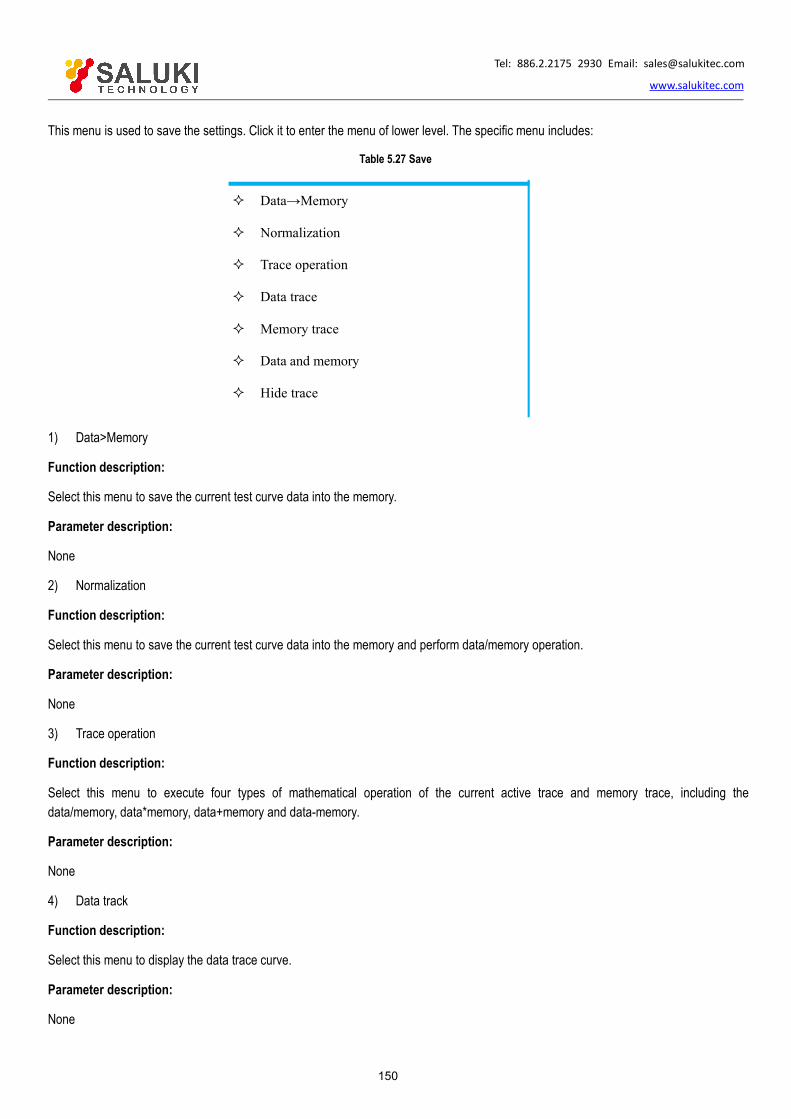
Tel: 886.2.2175 2930 Email: [email protected]
www.salukitec.com
150
This menu is used to save the settings. Click it to enter the menu of lower level. The specific menu includes:
Table 5.27 Save
Data→Memory
Normalization
Trace operation
Data trace
Memory trace
Data and memory
Hide trace
1) Data>Memory
Function description:
Select this menu to save the current test curve data into the memory.
Parameter description:
None
2) Normalization
Function description:
Select this menu to save the current test curve data into the memory and perform data/memory operation.
Parameter description:
None
3) Trace operation
Function description:
Select this menu to execute four types of mathematical operation of the current active trace and memory trace, including thedata/memory, data*memory, data+memory and data-memory.
Parameter description:
None
4) Data track
Function description:
Select this menu to display the data trace curve.
Parameter description:
None

Tel: 886.2.2175 2930 Email: [email protected]
www.salukitec.com
151
5) Memory trace
Function description:
Select this menu to display the memory trace Curve.
Parameter description:
None
6) Data and memory
Function description:
Select this menu to display the data trace and memory trace curve.
Parameter description:
None
7) Hide trace
Function description:
Select this menu to hide the data trace and memory trace.
Parameter description:
None
5.2.8.2. Test
This menu is used to set the test. Click it to enter the menu of lower level. The specific menu includes:
Table 5.28 Test
Limit test
Ripple test
Bandwidth test
1) Limit test
This menu is used to set the limit test. Click it to enter the menu of lower level. The specific menu includes:
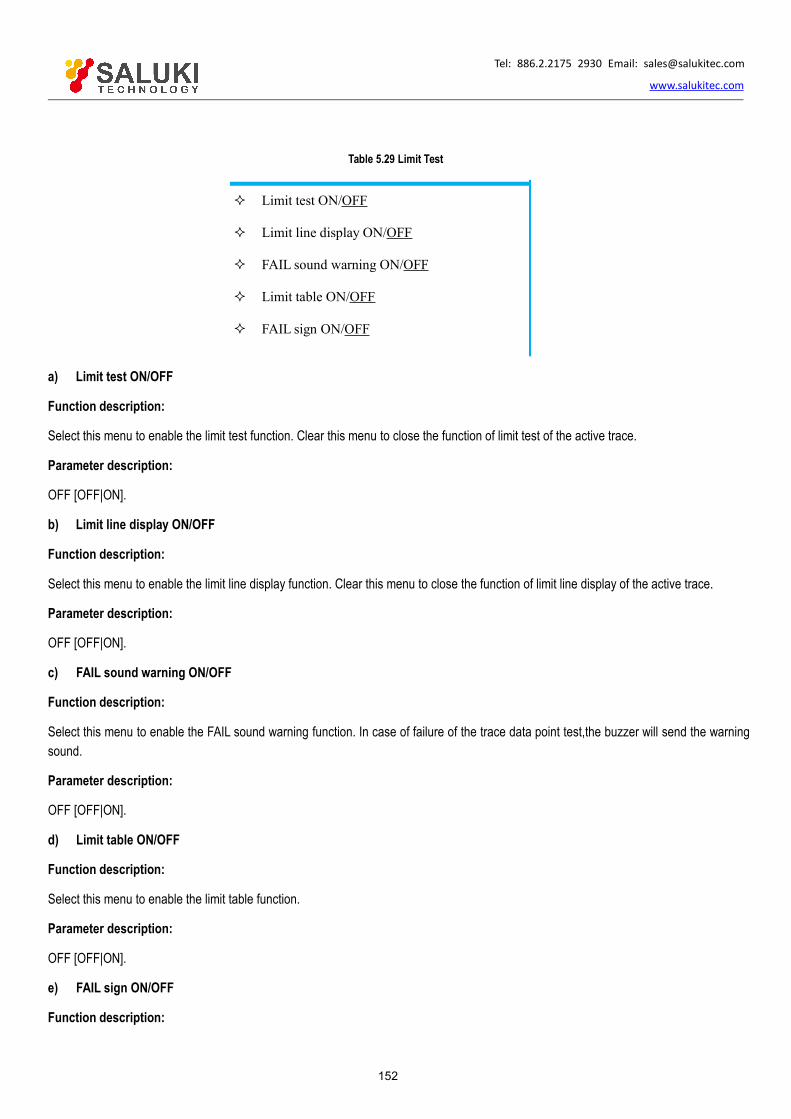
Tel: 886.2.2175 2930 Email: [email protected]
www.salukitec.com
152
Table 5.29 Limit Test
Limit test ON/OFF
Limit line display ON/OFF
FAIL sound warning ON/OFF
Limit table ON/OFF
FAIL sign ON/OFF
a) Limit test ON/OFF
Function description:
Select this menu to enable the limit test function. Clear this menu to close the function of limit test of the active trace.
Parameter description:
OFF [OFF|ON].
b) Limit line display ON/OFF
Function description:
Select this menu to enable the limit line display function. Clear this menu to close the function of limit line display of the active trace.
Parameter description:
OFF [OFF|ON].
c) FAIL sound warning ON/OFF
Function description:
Select this menu to enable the FAIL sound warning function. In case of failure of the trace data point test,the buzzer will send the warningsound.
Parameter description:
OFF [OFF|ON].
d) Limit table ON/OFF
Function description:
Select this menu to enable the limit table function.
Parameter description:
OFF [OFF|ON].
e) FAIL sign ON/OFF
Function description:
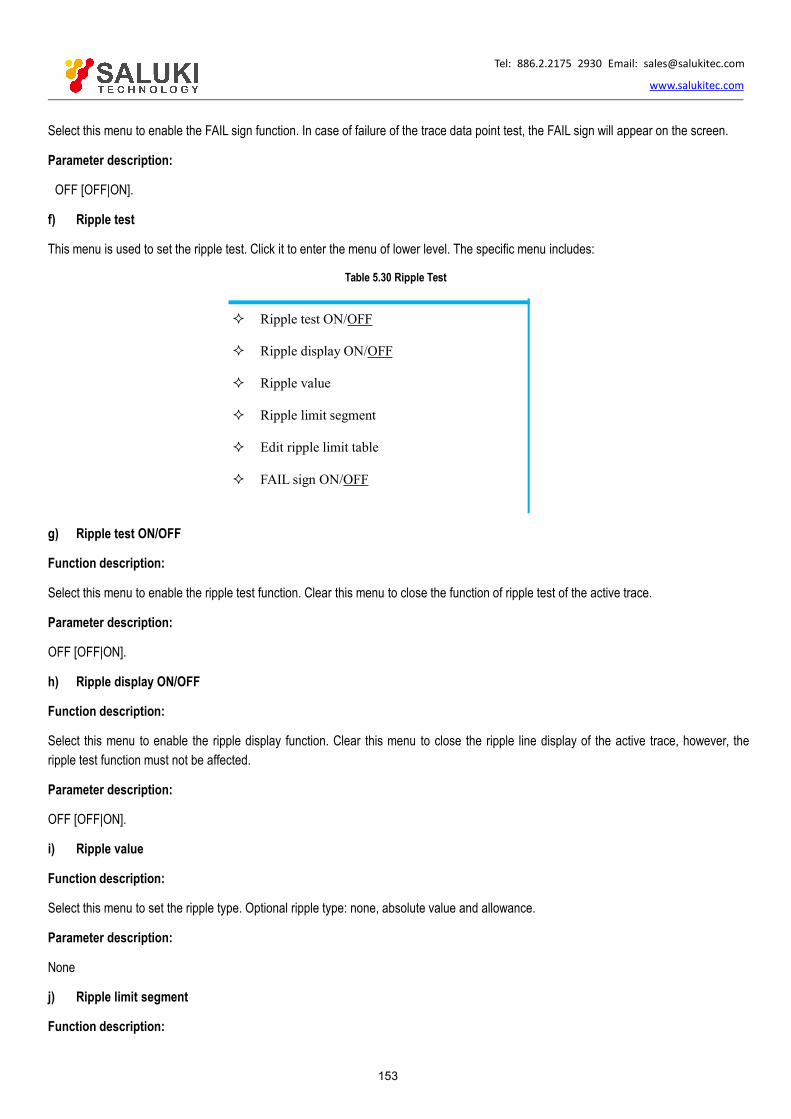
Tel: 886.2.2175 2930 Email: [email protected]
www.salukitec.com
153
Select this menu to enable the FAIL sign function. In case of failure of the trace data point test, the FAIL sign will appear on the screen.
Parameter description:
OFF [OFF|ON].
f) Ripple test
This menu is used to set the ripple test. Click it to enter the menu of lower level. The specific menu includes:
Table 5.30 Ripple Test
Ripple test ON/OFF
Ripple display ON/OFF
Ripple value
Ripple limit segment
Edit ripple limit table
FAIL sign ON/OFF
g) Ripple test ON/OFF
Function description:
Select this menu to enable the ripple test function. Clear this menu to close the function of ripple test of the active trace.
Parameter description:
OFF [OFF|ON].
h) Ripple display ON/OFF
Function description:
Select this menu to enable the ripple display function. Clear this menu to close the ripple line display of the active trace, however, theripple test function must not be affected.
Parameter description:
OFF [OFF|ON].
i) Ripple value
Function description:
Select this menu to set the ripple type. Optional ripple type: none, absolute value and allowance.
Parameter description:
None
j) Ripple limit segment
Function description:

Tel: 886.2.2175 2930 Email: [email protected]
www.salukitec.com
154
Select this menu to select the number of ripple limit segments to be opened. Up to 12 segments can be opened.
Parameter description:
None
k) Edit ripple limit table
Function description:
Select this menu to edit the ripple limit table. The ripple limit table can be added, deleted and edited.
Parameter description:
None
l) FAIL sign ON/OFF
Function description:
Select this menu to enable the FAIL sign function. In case of failure of the trace data point test, the FAIL sign will appear on the screen.
Parameter description:
OFF [OFF|ON].
2) Bandwidth test
This menu is used to set the bandwidth test. Click it to enter the menu of lower level. The specific menu includes:
Table 5.31 Bandwidth Test
Bandwidth test ON/OFF
Bandwidth display ON/OFF
Bandwidth marking ON/OFF
NdB point
Minimum bandwidth
Maximum bandwidth
FAIL sign ON/OFF
a) Bandwidth test ON/OFF
Function description:
Select this menu to enable the bandwidth test function to test the bandwidth of the bandpass filter.
Parameter description:
OFF [OFF|ON].
b) Bandwidth display ON/OFF
Function description:

Tel: 886.2.2175 2930 Email: [email protected]
www.salukitec.com
155
Select this menu to enable the bandwidth display function. The tested bandwidth will be displayed on the screen.
Parameter description:
OFF [OFF|ON].
c) Bandwidth marking ON/OFF
Function description:
Select this menu to enable the bandwidth marking function. The bandwidth position mark will be displayed on the screen.
Parameter description:
OFF [OFF|ON].
d) NdB point
Function description:
Select this menu to adjust the NdB point and determine the amplitude difference between two frequency points and the signal peak valueof the passband.
Parameter description:
-3dB [-500dB - 500dB].
e) Minimum bandwidth
Function description:
Select this menu to set the allowable minimum bandwidth. If the test bandwidth is less than the minimum value, the prompt of bandwidthtest failure (FAIL) will appear on the screen, or the prompt sound will be sent, so that the user can directly observe whether thecharacteristics of the tested device meet the requirements.
Parameter description:
10kHz [0Hz - 300kHz].
f) Maximum bandwidth
Function description:
Select this menu to set the allowable maximum bandwidth. If the test bandwidth exceeds the maximum value, the prompt of bandwidthtest failure (FAIL) will appear on the screen, or the prompt sound will be sent, so that the user can directly observe whether the testeddevice meet the requirements.
Parameter description:
300kHz [300kHz - ∞].
g) FAIL sign ON/OFF
Function description:
Select this menu to enable the FAIL sign function. In case of failure of the trace data point test, the FAIL sign will appear on the screen.
Parameter description:
OFF [OFF|ON].
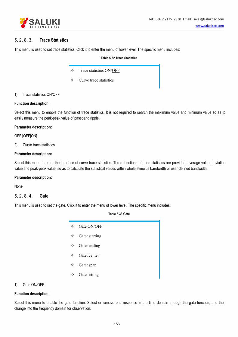
Tel: 886.2.2175 2930 Email: [email protected]
www.salukitec.com
156
5.2.8.3. Trace Statistics
This menu is used to set trace statistics. Click it to enter the menu of lower level. The specific menu includes:
Table 5.32 Trace Statistics
Trace statistics ON/OFF
Curve trace statistics
1) Trace statistics ON/OFF
Function description:
Select this menu to enable the function of trace statistics. It is not required to search the maximum value and minimum value so as toeasily measure the peak-peak value of passband ripple.
Parameter description:
OFF [OFF|ON].
2) Curve trace statistics
Parameter description:
Select this menu to enter the interface of curve trace statistics. Three functions of trace statistics are provided: average value, deviationvalue and peak-peak value, so as to calculate the statistical values within whole stimulus bandwidth or user-defined bandwidth.
Parameter description:
None
5.2.8.4. Gate
This menu is used to set the gate. Click it to enter the menu of lower level. The specific menu includes:
Table 5.33 Gate
Gate ON/OFF
Gate: starting
Gate: ending
Gate: center
Gate: span
Gate setting
1) Gate ON/OFF
Function description:
Select this menu to enable the gate function. Select or remove one response in the time domain through the gate function, and thenchange into the frequency domain for observation.

Tel: 886.2.2175 2930 Email: [email protected]
www.salukitec.com
157
Parameter description:
OFF [OFF|ON].
2) Gate: starting
Function description:
Select this menu to set the starting value of the gate.
Parameter description:
-10ns [-14.825797ns - 14.825797ns]
3) Gate: ending
Function description:
Select this menu to set the ending value of the gate.
Parameter description:
10ns [-14.825797ns - 14.825797ns]
4) Gate: center
Function description:
Select this menu to set the center value of the gate.
Parameter description:
0ns [-14.825797ns - 14.825797ns]
5) Gate: span
Function description:
Select this menu to set the span value of the gate.
Parameter description:
20ns [0ns-29.651594ns].
6) Gate: setting
Function description:
Select this menu to enter the window of time domain transformation function. The time domain transformation, gate, window and optionscan be set.
Parameter description:
None
5.2.8.5. Window
Function description:
Select this menu to enter the window of time domain transformation function. The time domain transformation, gate, window and optionscan be set.

Tel: 886.2.2175 2930 Email: [email protected]
www.salukitec.com
158
Parameter description:
None
5.2.8.6. Time domain
This menu is used to set the time domain. Click it to enter the menu of lower level. The specific menu includes:
Table 5.34 Time Domain
Time domain ON/OFF
Starting date
Ending time
Center time
Time span
Time domain transformation
Time domain window
Couple setting
Time domain toolbar
1) Time domain ON/OFF
Function description:
Select this menu to enable the time domain function.
Parameter description:
OFF [OFF|ON].
2) Starting date
Function description:
Select this menu to set the starting time.
Parameter description:
-10ns [-14.825797ns - 14.825797ns]
3) Ending time
Function description:
Select this menu to set the ending time.
Parameter description:
10ns [-14.825797ns - 14.825797ns]

Tel: 886.2.2175 2930 Email: [email protected]
www.salukitec.com
159
4) Center time
Function description:
Select this menu to set the center time.
Parameter description:
0ns [-14.825797ns - 14.825797ns]
5) Time span
Function description:
Select this menu to set the time span.
Parameter description:
20ns [0ns-29.651594ns].
6) Time domain transformation
Function description:
Select this menu to enter the window of time domain transformation function. The time domain transformation, gate, window and optionscan be set.
Parameter description:
None
7) Time domain window
Function description:
Select this menu to enter the window of time domain transformation function. The time domain transformation, gate, window and optionscan be set.
Parameter description:
None
8) Coupling setting
Function description:
Select this menu to enter the window of coupling setting function.
Parameter description:
None
9) Time domain toolbar
Function description:
Select this menu to enable the time domain toolbar function so as to clearly observe the influence of setting changes on measurement.
Parameter description:
OFF [OFF|ON].
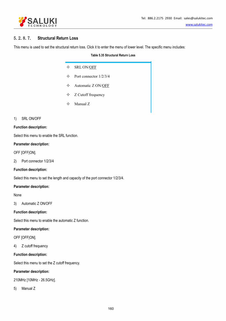
Tel: 886.2.2175 2930 Email: [email protected]
www.salukitec.com
160
5.2.8.7. Structural Return Loss
This menu is used to set the structural return loss. Click it to enter the menu of lower level. The specific menu includes:
Table 5.35 Structural Return Loss
SRLON/OFF
Port connector 1/2/3/4
Automatic Z ON/OFF
Z Cutoff frequency
Manual Z
1) SRL ON/OFF
Function description:
Select this menu to enable the SRL function.
Parameter description:
OFF [OFF|ON].
2) Port connector 1/2/3/4
Function description:
Select this menu to set the length and capacity of the port connector 1/2/3/4.
Parameter description:
None
3) Automatic Z ON/OFF
Function description:
Select this menu to enable the automatic Z function.
Parameter description:
OFF [OFF|ON].
4) Z cutoff frequency
Function description:
Select this menu to set the Z cutoff frequency.
Parameter description:
210MHz [10MHz - 26.5GHz].
5) Manual Z

Tel: 886.2.2175 2930 Email: [email protected]
www.salukitec.com
161
Function description:
Select this function to enable the manual Z function.
Parameter description:
OFF [OFF|ON].
5.2.8.8. Equation Editor
Function description:
Select this menu to enter the Equation Editor interface. Parameter description:
Parameter description:
OFF [OFF|ON].
5.2.9. System
Press the [System] key on the front panel or the [System] menu item on the user interface. The system-related menu will pop up. Specificitems include: [Configuration], [Record/Run 1], [Record/Run 2], [Windows task bar], [Reset], [Custom user reset state], [Language:CN/EN] and [Spread spectrum]. The specific description of menu items is as follows.
5.2.9.1. Configuration
This menu is used to set the configuration. Click it to enter the menu of lower level. The specific menu includes:
Table 5.36 Configuration
GPIB address
Control panel
System impedance
User configuration
Intermediate frequency selection
Millimeter wave module configuration
Expansion to 16 ports
Touch screen
1) GPIB address
Function description:
Select this menu to configure the GPIB address.
Parameter description:
16 [0 - 30].
2) Control panel

Tel: 886.2.2175 2930 Email: [email protected]
www.salukitec.com
162
Function description:
If this menu is selected, the control panel menu will pop up. The user can set the operating system.
Parameter description:
None
3) System impedance
Function description:
Select this menu to set the system impedance. The system impedance must be changed in measurements of devices except those of50Ω, such as waveguide devices.
Parameter description:
50Ω [0Ω-1kΩ].
4) User configuration
Function description:
If this menu is selected, the user can configure it. Configurable options include: "Enable touch screen", "Save calibration file in the currenttime name", "Not automatically save after calibration", "Display marker on all the existing tracks", "Display limit test on all the existingtracks", "Press the UP/DOWN key to change the marker point by point", "Install anti-virus software", "Multi-port calibration" and "Identifyport sweep state".
Parameter description:
None
5) Intermediate frequency selection
Function description:
Select this menu to select the IF, including the internal IF and external IF.
Parameter description:
None
6) Millimeter wave module configuration
Function description:
Select this menu to configure the millimeter wave module, including the model selection, port setting and frequency setting.
Parameter description:
None
7) Expansion to 16 ports
Function description:
Select this menu to expand the instrument to 16 ports.
Parameter description:
Tel: 886.2.2175 2930 Email: [email protected]
www.salukitec.com
163
None
8) Touch screen
Function description:
Select this menu to enable the touch screen function and calibrate the touch screen.
Parameter description:
None
5.2.9.2. Record/Run 1
Function description:
Select this menu to automatically start recording. If recording has been done, press this key to automatically start running.
Parameter description:
None
5.2.9.3. Record/Run 2
Function description:
Select this menu to automatically start recording. If recording has been done, press this key to automatically start running.
Parameter description:
None
5.2.9.4. Windows Task Bar
Function description:
Select this menu to open the operating system task bar.
Parameter description:
None
5.2.9.5. Reset
Function description:
Select this menu to run the application program of the S3602 series vector network analyzer.
Parameter description:
None
5.2.9.6. Reset User State
Function description:
Select this menu to customize the user state interface. The user can be customize the user reset state.
Parameter description:
Tel: 886.2.2175 2930 Email: [email protected]
www.salukitec.com
164
None
5.2.9.7. Spread Spectrum
Function description:
Select this menu to select the spread spectrum function, including SAV3644A, SAV3645A, SAV3646A, SAV3649, SAV3649A, etc.
Parameter description:
None
5.2.10. Help
Press the [Help] key on the front panel or the [Help] menu item on the user interface. The help-related menu will pop up. Specific itemsinclude: [Quick Start Manual], [Programming manual], [Technical support], [Error information] and [About]. The specific description ofmenu items is as follows.
5.2.10.1. Quick Start Manual
Function description:
Open the quick start manual
Parameter description:
None
5.2.10.2. Programming Manual
Function description:
Select this menu to open the Program Control Manual of S3602 Series Vector Network Analyzers.
Parameter description:
None
5.2.10.3. Technical Support
Function description:
Open the full user manual.
Parameter description:
None
5.2.10.4. Error Information
Function description:
Select this menu to select the error parameter and view the error log.
Parameter description:
None
5.2.10.5. About

Tel: 886.2.2175 2930 Email: [email protected]
www.salukitec.com
165
Function description:
Select this menu to view the basic information of the instrument and the company information.
Parameter description:
None

Tel: 886.2.2175 2930 Email: [email protected]
www.salukitec.com
166
6. Measurement OptimizationThe following methods can be applied to adjust the setting and optimize the measurement accuracy.
Reduction of accessory influence
Improvement of reflection accuracy of low-loss 2-port device
Increase of dynamic range
Improvement of measurement results of electrical long device
Improvement of phase measurement accuracy
Reduction of trace noise
Increase of data point number
Improvement of measurement stability
Improvement of sweep speed
Improvement of efficiency of multi-state measurement
Rapid data transmission
Macro use
6.1.Reduction of Accessory Influence
Some accessories may affect the measurement results of the tested device. Select one of two characteristics of the analyzer to reducethe accessory influence. In order to reduce the accessory influence, you can select the most suitable method to test the configuration.
1) Compensate the cable loss with the power slope.
If a long cable or other kind of accessory is used in measurement configuration, the power loss will be generated within the whole band.In this case, the power slope function should be applied. The defined ratio (dB/GHz) can be used in this function to increase the sourcepower of the analyzer. The process of cable loss compensation is as follows.
Menu path: [Stimulus] > [Power...].
If the power slope function is not activated, tick the [Slope] check box. Input the ratio to be increased in frequency sweep of the sourcepower in the [dB/GHz] box.
2) Selectively remove the response gate (only for the time domain).
a) The gate is one of the time domain characteristics. It is used to remove the response mathematically. The gate of reflectionresponse or transmission response can be set, but different results will be obtained.
Gate reflection response: the desired response (such as the return loss of the filter) can be separated from the undesiredresponse (such as the adapter reflection or connector mismatch) by reflection response of the gate.
Gate transmission response: the specific path of large electrical length in the multi-path device can be separated bytransmission response of the gate.
In order to apply the gate in the time domain mode, the transformation can be disconnected, and the existing gate pulse can be usedin study of the frequency response of the device. The time filter gate pulse have the following shapes and features:
Band pass shape: the response beyond the passband zone can be removed.
Trap shape: unnecessary response in the frequency zone can be removed.
b) Removal of unnecessary response
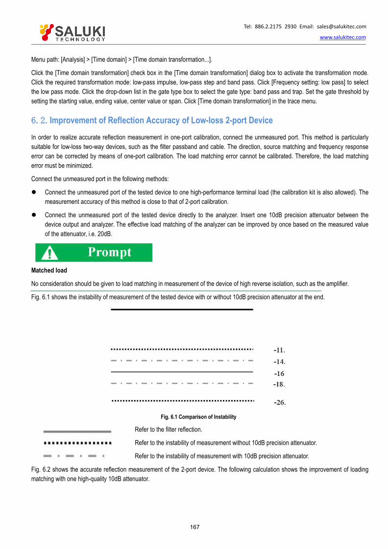
Tel: 886.2.2175 2930 Email: [email protected]
www.salukitec.com
167
Menu path: [Analysis] > [Time domain] > [Time domain transformation...].
Click the [Time domain transformation] check box in the [Time domain transformation] dialog box to activate the transformation mode.Click the required transformation mode: low-pass impulse, low-pass step and band pass. Click [Frequency setting: low pass] to selectthe low pass mode. Click the drop-down list in the gate type box to select the gate type: band pass and trap. Set the gate threshold bysetting the starting value, ending value, center value or span. Click [Time domain transformation] in the trace menu.
6.2.Improvement of Reflection Accuracy of Low-loss 2-port Device
In order to realize accurate reflection measurement in one-port calibration, connect the unmeasured port. This method is particularlysuitable for low-loss two-way devices, such as the filter passband and cable. The direction, source matching and frequency responseerror can be corrected by means of one-port calibration. The load matching error cannot be calibrated. Therefore, the load matchingerror must be minimized.
Connect the unmeasured port in the following methods:
Connect the unmeasured port of the tested device to one high-performance terminal load (the calibration kit is also allowed). Themeasurement accuracy of this method is close to that of 2-port calibration.
Connect the unmeasured port of the tested device directly to the analyzer. Insert one 10dB precision attenuator between thedevice output and analyzer. The effective load matching of the analyzer can be improved by once based on the measured valueof the attenuator, i.e. 20dB.
Matched load
No consideration should be given to load matching in measurement of the device of high reverse isolation, such as the amplifier.
Fig. 6.1 shows the instability of measurement of the tested device with or without 10dB precision attenuator at the end.
Fig. 6.1 Comparison of Instability
Refer to the filter reflection.
Refer to the instability of measurement without 10dB precision attenuator.
Refer to the instability of measurement with 10dB precision attenuator.
Fig. 6.2 shows the accurate reflection measurement of the 2-port device. The following calculation shows the improvement of loadingmatching with one high-quality 10dB attenuator.
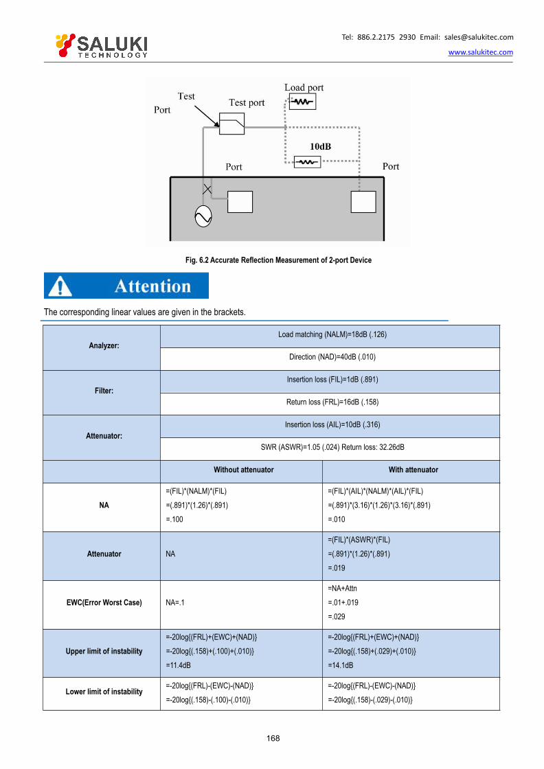
Tel: 886.2.2175 2930 Email: [email protected]
www.salukitec.com
168
Fig. 6.2 Accurate Reflection Measurement of 2-port Device
The corresponding linear values are given in the brackets.
Analyzer:Load matching (NALM)=18dB (.126)
Direction (NAD)=40dB (.010)
Filter:Insertion loss (FIL)=1dB (.891)
Return loss (FRL)=16dB (.158)
Attenuator:Insertion loss (AIL)=10dB (.316)
SWR (ASWR)=1.05 (.024) Return loss: 32.26dB
Without attenuator With attenuator
NA=(FIL)*(NALM)*(FIL)=(.891)*(1.26)*(.891)=.100
=(FIL)*(AIL)*(NALM)*(AIL)*(FIL)=(.891)*(3.16)*(1.26)*(3.16)*(.891)=.010
Attenuator NA=(FIL)*(ASWR)*(FIL)=(.891)*(1.26)*(.891)=.019
EWC(Error Worst Case) NA=.1=NA+Attn=.01+.019=.029
Upper limit of instability=-20log(FRL)+(EWC)+(NAD)=-20log(.158)+(.100)+(.010)=11.4dB
=-20log(FRL)+(EWC)+(NAD)=-20log(.158)+(.029)+(.010)=14.1dB
Lower limit of instability=-20log(FRL)-(EWC)-(NAD)=-20log(.158)-(.100)-(.010)
=-20log(FRL)-(EWC)-(NAD)=-20log(.158)-(.029)-(.010)
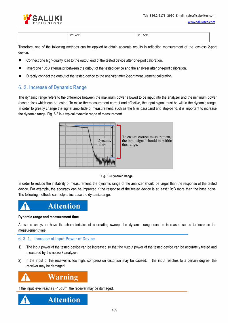
Tel: 886.2.2175 2930 Email: [email protected]
www.salukitec.com
169
=26.4dB =18.5dB
Therefore, one of the following methods can be applied to obtain accurate results in reflection measurement of the low-loss 2-portdevice.
Connect one high-quality load to the output end of the tested device after one-port calibration.
Insert one 10dB attenuator between the output of the tested device and the analyzer after one-port calibration.
Directly connect the output of the tested device to the analyzer after 2-port measurement calibration.
6.3.Increase of Dynamic Range
The dynamic range refers to the difference between the maximum power allowed to be input into the analyzer and the minimum power(base noise) which can be tested. To make the measurement correct and effective, the input signal must be within the dynamic range.In order to greatly change the signal amplitude of measurement, such as the filter passband and stop-band, it is important to increasethe dynamic range. Fig. 6.3 is a typical dynamic range of measurement.
Fig. 6.3 Dynamic Range
In order to reduce the instability of measurement, the dynamic range of the analyzer should be larger than the response of the testeddevice. For example, the accuracy can be improved if the response of the tested device is at least 10dB more than the base noise.The following methods can help to increase the dynamic range.
Dynamic range and measurement time
As some analyzers have the characteristics of alternating sweep, the dynamic range can be increased so as to increase themeasurement time.
6.3.1. Increase of Input Power of Device
1) The input power of the tested device can be increased so that the output power of the tested device can be accurately tested andmeasured by the network analyzer.
2) If the input of the receiver is too high, compression distortion may be caused. If the input reaches to a certain degree, thereceiver may be damaged.
If the input level reaches +15dBm, the receiver may be damaged.
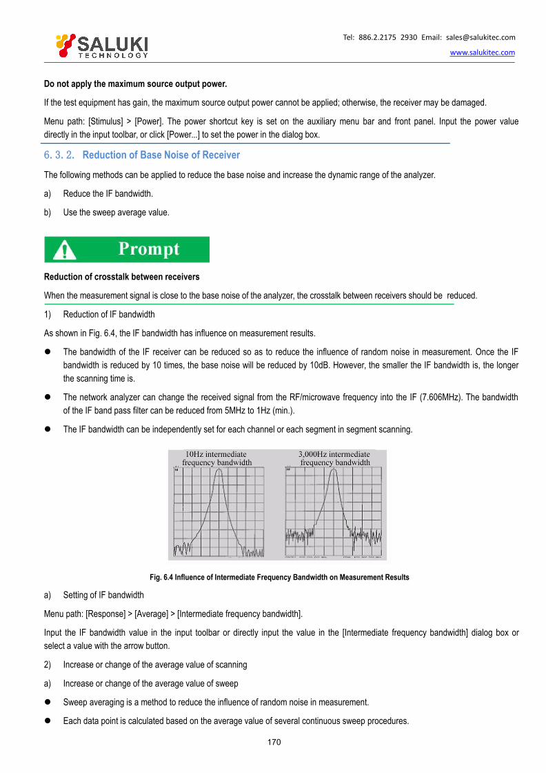
Tel: 886.2.2175 2930 Email: [email protected]
www.salukitec.com
170
Do not apply the maximum source output power.
If the test equipment has gain, the maximum source output power cannot be applied; otherwise, the receiver may be damaged.
Menu path: [Stimulus] > [Power]. The power shortcut key is set on the auxiliary menu bar and front panel. Input the power valuedirectly in the input toolbar, or click [Power...] to set the power in the dialog box.
6.3.2. Reduction of Base Noise of Receiver
The following methods can be applied to reduce the base noise and increase the dynamic range of the analyzer.
a) Reduce the IF bandwidth.
b) Use the sweep average value.
Reduction of crosstalk between receivers
When the measurement signal is close to the base noise of the analyzer, the crosstalk between receivers should be reduced.
1) Reduction of IF bandwidth
As shown in Fig. 6.4, the IF bandwidth has influence on measurement results.
The bandwidth of the IF receiver can be reduced so as to reduce the influence of random noise in measurement. Once the IFbandwidth is reduced by 10 times, the base noise will be reduced by 10dB. However, the smaller the IF bandwidth is, the longerthe scanning time is.
The network analyzer can change the received signal from the RF/microwave frequency into the IF (7.606MHz). The bandwidthof the IF band pass filter can be reduced from 5MHz to 1Hz (min.).
The IF bandwidth can be independently set for each channel or each segment in segment scanning.
Fig. 6.4 Influence of Intermediate Frequency Bandwidth on Measurement Results
a) Setting of IF bandwidth
Menu path: [Response] > [Average] > [Intermediate frequency bandwidth].
Input the IF bandwidth value in the input toolbar or directly input the value in the [Intermediate frequency bandwidth] dialog box orselect a value with the arrow button.
2) Increase or change of the average value of scanning
a) Increase or change of the average value of sweep
Sweep averaging is a method to reduce the influence of random noise in measurement.
Each data point is calculated based on the average value of several continuous sweep procedures.
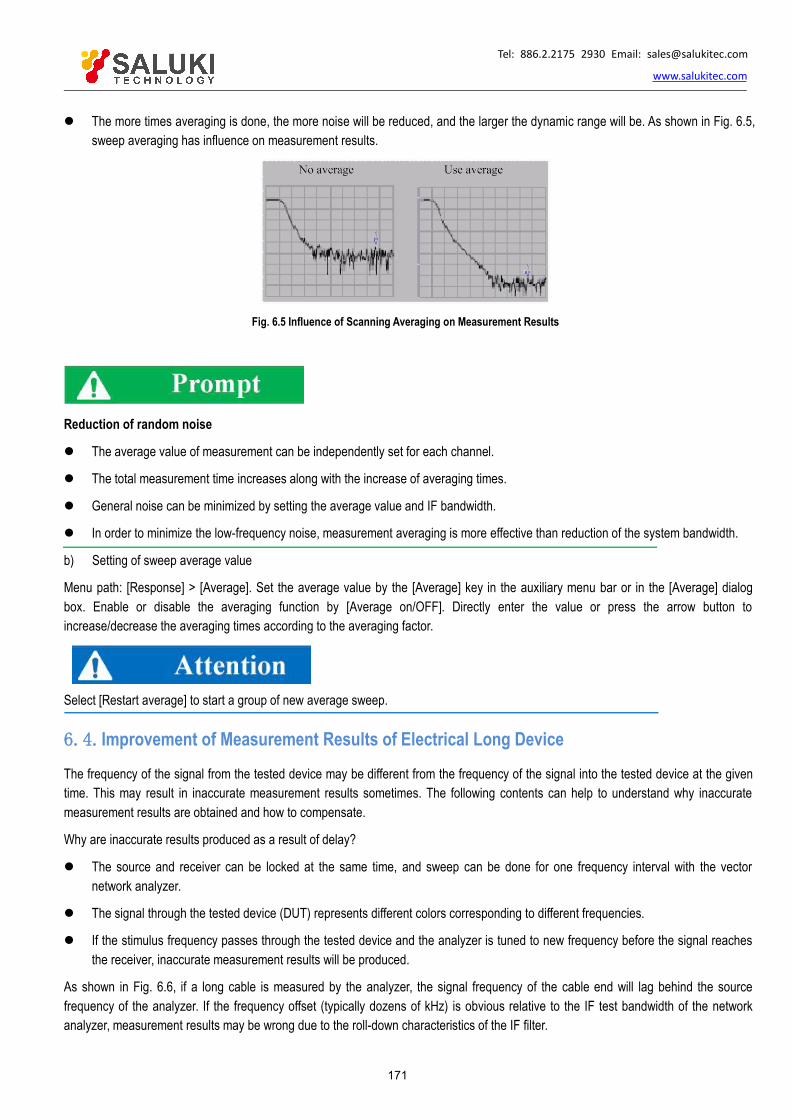
Tel: 886.2.2175 2930 Email: [email protected]
www.salukitec.com
171
The more times averaging is done, the more noise will be reduced, and the larger the dynamic range will be. As shown in Fig. 6.5,sweep averaging has influence on measurement results.
Fig. 6.5 Influence of Scanning Averaging on Measurement Results
Reduction of random noise
The average value of measurement can be independently set for each channel.
The total measurement time increases along with the increase of averaging times.
General noise can be minimized by setting the average value and IF bandwidth.
In order to minimize the low-frequency noise, measurement averaging is more effective than reduction of the system bandwidth.
b) Setting of sweep average value
Menu path: [Response] > [Average]. Set the average value by the [Average] key in the auxiliary menu bar or in the [Average] dialogbox. Enable or disable the averaging function by [Average on/OFF]. Directly enter the value or press the arrow button toincrease/decrease the averaging times according to the averaging factor.
Select [Restart average] to start a group of new average sweep.
6.4.Improvement of Measurement Results of Electrical Long Device
The frequency of the signal from the tested device may be different from the frequency of the signal into the tested device at the giventime. This may result in inaccurate measurement results sometimes. The following contents can help to understand why inaccuratemeasurement results are obtained and how to compensate.
Why are inaccurate results produced as a result of delay?
The source and receiver can be locked at the same time, and sweep can be done for one frequency interval with the vectornetwork analyzer.
The signal through the tested device (DUT) represents different colors corresponding to different frequencies.
If the stimulus frequency passes through the tested device and the analyzer is tuned to new frequency before the signal reachesthe receiver, inaccurate measurement results will be produced.
As shown in Fig. 6.6, if a long cable is measured by the analyzer, the signal frequency of the cable end will lag behind the sourcefrequency of the analyzer. If the frequency offset (typically dozens of kHz) is obvious relative to the IF test bandwidth of the networkanalyzer, measurement results may be wrong due to the roll-down characteristics of the IF filter.

Tel: 886.2.2175 2930 Email: [email protected]
www.salukitec.com
172
Fig. 6.6 Schematic Diagram of Test of Long Cable
The delay of the electrical long device can be compensated in the following methods.
1) Reduction of sweep speed
The sweep speed can be reduced by increasing the scanning time, reducing the IF bandwidth or increasing the number of sweeppoints.
a) Increase the sweep time.
Menu path: [Stimulus] > [Sweep] > [Sweep time...]. Enter the time or select the time with the arrow.
b) Reduce the IF bandwidth.
Menu path: [Response] > [Average] > [Intermediate frequency bandwidth...]. Directly enter the value or select the time with the arrow.
c) Increase the number of sweep points.
Menu path: [Stimulus] > [Sweep] > [Number of sweep points].
Directly click the required point number in the sub-menu or click [Custom...]. Enter the value in the [Number of sweep points] dialogbox or select the value with the arrow.
2) Use of step sweep.
Change analog sweep into step sweep so that the source can step over each test point. In this case, the
sweep speed of the analyzer can be reduced. The dwell time of each step or test point can also be set. Menu path: [Stimulus] >[Sweep] > [Sweep setting...].
Tick the step sweep Directly enter the dwell time in the [dwell time] box or select the required dwell time
of each test point.
6.5.Improvement of Phase Measurement Accuracy
The following characteristics of the analyzer can be applied to improve the accuracy of phase measurement.
Electrical delay
Port extension
phase offset
Frequency point interval
Specific operation
6.5.1. Electrical Delay
The electrical delay can be applied to compensate the linear phase offset of the tested device so as to highlight the linear phaseoffset of the tested device.
Tel: 886.2.2175 2930 Email: [email protected]
www.salukitec.com
173
The electrical delay is a kind of mathematical function. The transmission line of no loss and adjustable length can be simulated.
The electrical delay which is not associated with each measurement trace can be set.
6.5.2. Port Extension1) The measurement reference plane can be moved electrically by means of port extension after calibration. Thus, other kinds of
calibration can be avoided. Port extension is introduced in the following two cases.
a) Decide whether to add one cable in the measurement configuration after calibration. The port extension characteristics canbe applied to “tell' the analyzer to increase the cable length to the specific port.
b) If calibration cannot be done directly on the tested device in the test fixture, port extension can be applied to compensatethe delay (phase offset) arising from the fixture.
2) Use of port extension function
a) If the electrical length of the tested fixture or added cable is known, enter the value in the [Time] box.
b) If the physical length of the tested fixture or added cable is known, enter the value in the [Distance] box.
c) If the above two items are unknown, the open-circuit device or short-circuit device can be used instead of the tested deviceon the reference plane after extension. Generally, the new reference plane is regarded in the open- circuit state afterremoval of the tested device.
3) The appropriate port extension value can be obtained in the following methods.
a) Select the S11 measurement after calibration and set the phase format as the display format.
b) Connect the open-circuit device or short-circuit device to the calibration plane and check whether the displayed phase curveis within the measurement frequency range and around 0°.
c) Connect the fixture or transmission cable and use the open-circuit device or short-circuit device instead of the tested device(the circuit is regarded as an open circuit if the tested device is removed). Adjust the value of
d) the [Time] or [Distance] box in the [Port extension] dialog box until the phase trace is flat.
e) If the loss characteristics of the extension part are known, compensation can be done in the one-dimensional ortwo-dimensional manner in the [Loss compensation] part.
Nonzero delay
The nonzero delay is specified in the majority of short circuit standards and can be applied to adjust the error which is twice that ofshort-circuit calibration as a result of port extension and further view the definition of the calibration kit so as to determine theappropriate extension value.
4) Setting of port extension
Menu path: [Calibration] > [Port extension].
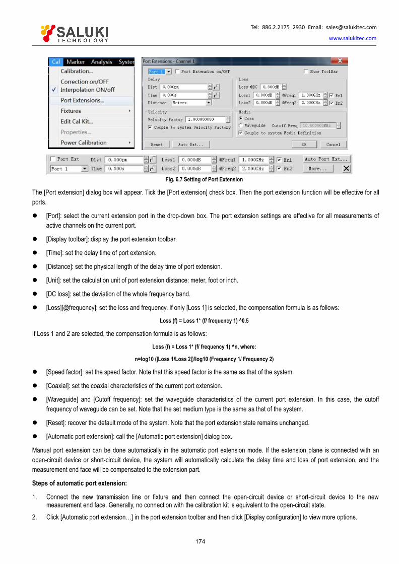
Tel: 886.2.2175 2930 Email: [email protected]
www.salukitec.com
174
Fig. 6.7 Setting of Port Extension
The [Port extension] dialog box will appear. Tick the [Port extension] check box. Then the port extension function will be effective for allports.
[Port]: select the current extension port in the drop-down box. The port extension settings are effective for all measurements ofactive channels on the current port.
[Display toolbar]: display the port extension toolbar.
[Time]: set the delay time of port extension.
[Distance]: set the physical length of the delay time of port extension.
[Unit]: set the calculation unit of port extension distance: meter, foot or inch.
[DC loss]: set the deviation of the whole frequency band.
[Loss][@frequency]: set the loss and frequency. If only [Loss 1] is selected, the compensation formula is as follows:
Loss (f) = Loss 1* (f/ frequency 1) ^0.5
If Loss 1 and 2 are selected, the compensation formula is as follows:
Loss (f) = Loss 1* (f/ frequency 1) ^n, where:
n=log10 (|Loss 1/Loss 2|)/log10 (Frequency 1/ Frequency 2)
[Speed factor]: set the speed factor. Note that this speed factor is the same as that of the system.
[Coaxial]: set the coaxial characteristics of the current port extension.
[Waveguide] and [Cutoff frequency]: set the waveguide characteristics of the current port extension. In this case, the cutofffrequency of waveguide can be set. Note that the set medium type is the same as that of the system.
[Reset]: recover the default mode of the system. Note that the port extension state remains unchanged.
[Automatic port extension]: call the [Automatic port extension] dialog box.
Manual port extension can be done automatically in the automatic port extension mode. If the extension plane is connected with anopen-circuit device or short-circuit device, the system will automatically calculate the delay time and loss of port extension, and themeasurement end face will be compensated to the extension part.
Steps of automatic port extension:
1. Connect the new transmission line or fixture and then connect the open-circuit device or short-circuit device to the newmeasurement end face. Generally, no connection with the calibration kit is equivalent to the open-circuit state.
2. Click [Automatic port extension…] in the port extension toolbar and then click [Display configuration] to view more options.

Tel: 886.2.2175 2930 Email: [email protected]
www.salukitec.com
175
3. Click [Measurement] to start the port extension calculation. The calculated delay time and loss value will be automaticallydisplayed in the toolbar.
Fig. 6.8 Automatic Port Extension
[Open circuit] and [Short circuit]: connect the open-circuit device or short-circuit device to the port requiring automatic extension.
[Display configuration] and [Hide configuration]: display and hide the configuration of automatic port extension.
Measurement port number: select the port to be subject to automatic extension calculation.
Method: set the frequency range of the data collected for automatic port extension calculation.
[Default range]: the same as the frequency range of current measurement.
[Activate marker]: use the data between the activated marker and the part of the highest frequency to calculate the automaticport extension.
[User-defined]: the user enters the frequency range of calculation.
[Include loss]: select it to automatically calculate the loss arising from the current port extension.
[Compensation mismatch]: select it to automatically compensate the error arising from mismatch.
[Prompt of calibration kit connection]: if this item is selected, the [Calculation kit connection] prompt box will pop up.
[Close]: apply the current calculation results to the active channel and exit the dialog box.
6.5.3. phase offsetThe phase offset is a kind of mathematical phase measurement, and the deviation range is 0-360°. Use this characteristic in thefollowing methods:
Improve the display of phase measurement results.
This is similar to the improvement of reference level in amplitude measurement. Change the phase response to make it at the screencenter or on the same straight line as the screen.
Simulate the phase offset determined in measurement.
For example, if it is known to add a cable and the cable length may result in phase offset of measurement results, the phase offset canbe increased by movement and the measurement of the whole device can be simulated.
1) Setting of phase offset
Menu path: [Response] > [Scale] > [phase offset...]. The [phase offset] dialog box will appear.
Set the phase offset in the [phase offset] box.

Tel: 886.2.2175 2930 Email: [email protected]
www.salukitec.com
176
Fig. 6.9 Automatic Port Extension
6.5.4. Frequency Point Interval1) Sample the data of discrete frequency points, connect each sampling point and form a trace on the screen.
2) If the phase offset of two adjacent frequency points of the device is more than 180°, the displayed phase slope will look like thereverse phase. This is caused by mixing as a result of insufficient data sampling.
If the group delay is measured but the phase slope is opposite, the symbol will be changed as a result of the group delay. For example,Fig. 6.10 shows the measurement results of the surface acoustic wave (SAW) bandpass filter.
a) The first figure shows the measurement results of 51 points, and the group delay is negative. But this is impossible in the actualsituation, as the response will not be below the reference line (0s).
b) The second figure shows the measurement results of 201 points, and the group delay is positive, that is, the response is abovethe reference line (0s).
Fig. 6.10 Influence of Frequency Interval on Phase Measurement
Mixing check
In order to check mixing in measurement, you can check whether the display data change by reducing the frequency interval. You canincrease the number of frequency points or reduce the frequency interval to avoid mixing.
6.5.5. Specific Operations1) Compensation of linear phase offset
Menu path: [Response] > [Scale] > [Electrical delay...].
Enter the required value in the [Electrical delay] box or select the value with the arrow.
Enter the value in the [Speed factor] box or select the value between 0 and 1.0 with the arrow.
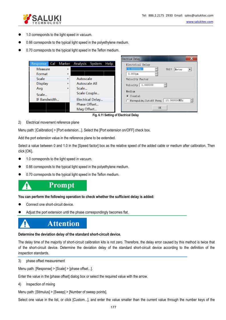
Tel: 886.2.2175 2930 Email: [email protected]
www.salukitec.com
177
1.0 corresponds to the light speed in vacuum.
0.66 corresponds to the typical light speed in the polyethylene medium.
0.70 corresponds to the typical light speed in the Teflon medium.
Fig. 6.11 Setting of Electrical Delay
2) Electrical movement reference plane
Menu path: [Calibration] > [Port extension...]. Select the [Port extension on/OFF] check box.
Add the port extension value in the reference plane to be extended.
Select a value between 0 and 1.0 in the [Speed factor] box as the relative speed of the added cable or medium after calibration. Thenclick [OK].
1.0 corresponds to the light speed in vacuum.
0.66 corresponds to the typical light speed in the polyethylene medium.
0.70 corresponds to the typical light speed in the Teflon medium.
You can perform the following operation to check whether the sufficient delay is added:
Connect one short-circuit device.
Adjust the port extension until the phase correspondingly becomes flat.
Determine the deviation delay of the standard short-circuit device.
The delay time of the majority of short-circuit calibration kits is not zero. Therefore, the delay error caused by this method is twice thatof the short-circuit device. Determine the deviation delay of the standard short-circuit device according to the definition of theinspection standards.
3) phase offset measurement
Menu path: [Response] > [Scale] > [phase offset...].
Enter the value in the [phase offset] dialog box or select the required value with the arrow.
4) Inspection of mixing
Menu path: [Stimulus] > [Sweep] > [Number of sweep points].
Select one value in the list, or click [Custom...], and enter the value smaller than the current value through the number keys of the
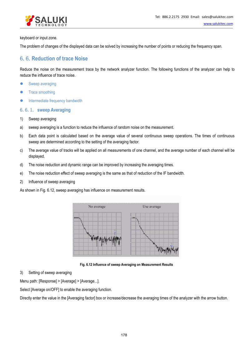
Tel: 886.2.2175 2930 Email: [email protected]
www.salukitec.com
178
keyboard or input zone.
The problem of changes of the displayed data can be solved by increasing the number of points or reducing the frequency span.
6.6.Reduction of trace Noise
Reduce the noise on the measurement trace by the network analyzer function. The following functions of the analyzer can help toreduce the influence of trace noise.
Sweep averaging
Trace smoothing
Intermediate frequency bandwidth
6.6.1. sweep Averaging1) Sweep averaging
a) sweep averaging is a function to reduce the influence of random noise on the measurement.
b) Each data point is calculated based on the average value of several continuous sweep operations. The times of continuoussweep are determined according to the setting of the averaging factor.
c) The average value of tracks will be applied on all measurements of one channel, and the average number of each channel will bedisplayed.
d) The noise reduction and dynamic range can be improved by increasing the averaging times.
e) The noise reduction effect of sweep averaging is the same as that of reduction of the IF bandwidth.
2) Influence of sweep averaging
As shown in Fig. 6.12, sweep averaging has influence on measurement results.
Fig. 6.12 Influence of sweep Averaging on Measurement Results
3) Setting of sweep averaging
Menu path: [Response] > [Average] > [Average...].
Select [Average on/OFF] to enable the averaging function.
Directly enter the value in the [Averaging factor] box or increase/decrease the averaging times of the analyzer with the arrow button.

Tel: 886.2.2175 2930 Email: [email protected]
www.salukitec.com
179
Fig. 6.13 Setting of sweep Averaging
Click [Restart average] in the sub-menu to start a group of new average sweep.
6.6.2. Trace SmoothingThe smoothing function is used to reduce the peak-peak noise of broadband measurement data. The data of part of the displayedtrace are averaged by the analyzer. The number of adjacent data points subject to averaging at the same time is also known as thesmoothing aperture. The aperture can be defined as the number of data point or the percentage of X-axis span.
Use of the smoothing function:
Use sufficient points in the display to avoid misleading results.
The smoothing function must not be applied to the highly resonant device or the device subject to broad track changes, asmeasurement errors may be caused.
The smoothing function can be independently set for each trace.
1) Influence of trace smoothing
Fig. 6.14 Influence of trace Smoothing on Measurement Results
2) Setting of trace smoothing
Menu path: [Response] > [Average] > [Smooth...].
Click [Smooth] to enable the smoothing function.
Select the method to specify the value of the smoothing aperture:
a) Enter the smoothing percentage in the [Smoothing percentage] box. (Max. 25%)
b) Enter the number of smoothing points in the [Number of smoothing points] box. (The maximum value is 25% of the total number

Tel: 886.2.2175 2930 Email: [email protected]
www.salukitec.com
180
of scanning points of the test.)
Fig. 6.15 Setting of Smoothing
6.6.3. Intermediate Frequency BandwidthYou can reduce the bandwidth of the IF receiver so as to reduce the influence of random noise in measurement. Once the IFbandwidth is reduced by 10 times, the base noise will be reduced by 10dB. However, if the IF bandwidth is small, the sweep time willbe long. The signal received by the analyzer will be changed into the IF (7.606MHz) from the network analyzer can change thereceived signal from the RF/microwave frequency into the IF (7.606MHz). The bandwidth of the IF band pass filter can be reducedfrom 5MHz to 1Hz (min.). The IF bandwidth can be independently set for each channel or in segment sweep.
1) Reduction of influence of IF bandwidth
The influence of the IF bandwidth on measurement results is shown in Fig. 6.16.
Fig. 6.16 Influence of Intermediate Frequency Bandwidth on Measurement Results
2) Setting of IF bandwidth
Menu path: [Response] > [Average] > [Intermediate frequency bandwidth...].
Directly enter the value in the [Intermediate frequency bandwidth] dialog box or select the value with the arrow button.
Fig. 6.17 Setting of Intermediate Frequency Bandwidth

Tel: 886.2.2175 2930 Email: [email protected]
www.salukitec.com
181
6.7.Increase of Data Point Number
The data point or 'point' refers to the sampling results of next value after one stimulus. You can define the number of measurementpoints within one sweep.
The trace can be scanned through a large number of data points so as to better define the device response.
The majority of data processing is done between adjacent points. One "sweep" refers to the measurement results of a series ofcontinuous data points, corresponding to the stimulus value within one sequence.
The default number of points of each sweep is 201.
The sweep time of the analyzer can be changed according to the number of sweep points and the scale. However, the totalmeasurement period will not change according to the number of sweep points and the scale. Instead, it is affected by other factors,such as the flyback time, data calculation, formation time, etc. Refer to the technical specifications for the influence of the point numberand other settings on the sweep time.
Use of data points
In order to obtain the best trace resolution, use the maximum number of data points.
In order to realize rapid throughput, use the minimum number of data points, which can help to achieve the acceptable accuracy.
In order to find the optimal number of data points, find a value with measurement results subject to no significant difference fromthe required number of measurement points.
In order to ensure the accurate measurement calibration, the number of calibration points should be the same as that ofmeasurement points.
1) Specific operations
Menu path: [Stimulus] > [Sweep] > [Number of sweep points].
Directly click the required point number in the [Number of sweep points] sub-menu, or click [Custom...], enter the value in the [Numberof sweep points] dialog box, or select the value with the arrow.

Tel: 886.2.2175 2930 Email: [email protected]
www.salukitec.com
182
Fig. 6.18 Setting of Number of sweep Points
2) Optimization of measurement results
One measurement includes several interdependent settings. You can modify the settings to achieve the purposes of measurementapplication: faster throughput or more accurate data. You can balance the settings to optimize measurement.
Increase the measurement throughput.
Improve the measurement accuracy.
6.8.Improvement of Measurement Stability
Measurement instability is caused under several conditions. For repeated measurement, you can apply several methods to create astable measurement environment. The following factors have adverse effects on the measurement accuracy.
1) frequency offset
The frequency precision of the analyzer depends on the accuracy of the internal 10MHZ oscillator. If high frequency accuracy andstability are required in the measurement application, no consideration should be given to the internal frequency standard, and ahigh-stability external frequency source can be created by the 10MHz reference input connector on the rear panel.
2) Temperature deviation
a) The electrical characteristics of the following components can be changed as a result of thermal expansion and contraction.
Internal device of analyzer
Standard of calibration kit
Tester
Cable
Adapter
b) The temperature deviation in measurement can be reduced in the following methods.
Tel: 886.2.2175 2930 Email: [email protected]
www.salukitec.com
183
Apply a temperature-controlled environment.
Ensure the temperature stability of the calibration kit.
Avoid unnecessary operation of the calibration kit during calibration.
Ensure that the difference between the ambient temperature and calibration temperature is ±1.
3) Improper measurement calibration
Improper measurement calibration may result in failure to detect the correct response of the tested device. You can apply the followingmethods to ensure the proper calibration:
a) Perform the measurement calibration of the connection of the tested device, i.e. reference plane.
b) If an additional accessory (cable, adapter or attenuator) is inserted into the tested device after one measurement calibration, theadditional electrical length and delay time can be compensated by the port extension function.
c) Apply the calibration standard defined in the calibration process. For more details, see the section about accurate measurementcalibration.
4) Equipment connector
A good connector is necessary in repeated measurement. Good connection can be realized in the following methods:
a) Check and clean the connectors of all components in the test equipment.
b) Apply the correct connection method.
c) Do not move the cable during measurement.
5) Apply the external reference frequency.
Input the external frequency reference signal to the rear panel connector.
a) Input frequency: 10MHz±10ppm
b) Input level: -15dBm to +20dBm
c) Input impedance: 200ohms
6) Control the room temperature.
a) Run the analyzer for more than 30min before each measurement calibration or equipment measurement.
b) Measure the equipment in the temperature-controlled environment. All the instructions and characteristics are applied at23±3 (unless otherwise specified).
c) Ensure that the difference between the ambient temperature and calibration temperature is ±1.
7) Stabilize the standard temperature of calibration.
a) Open the calibration kit box and take out the standard kit out of the protective foam one hour before measurement calibration.
b) Avoid unnecessary operation of the calibration kit in each measurement calibration.
8) Use connectors in good conditions.
a) Check all connectors with the magnifying glass. Check the following kinds of damage: wear, bending, breakage, deep scratch,dent, rounded shoulder, dirt or metal chippings.
b) Clean all connectors with isopropyl alcohol and swabs.
Evaporate alcohol.
Gradually dry connectors with compressed air.

Tel: 886.2.2175 2930 Email: [email protected]
www.salukitec.com
184
c) Properly connect the parts.
Connect the body and other parts to the ground with anti-static pads and wrist straps.
Arrange the connectors in one row.
Rotate the connection nuts.
Perform final connection with the torque wrench.
6.9.Increase of sweep Speed
The measurement efficiency can be improved by increasing the sweep speed. The highest scanning speed can be achieved byoptimizing the following settings in measurement.
1) sweep setting
Carefully set the following items to achieve the highest sweep speed.
Frequency span: only measure the frequency range of the tested device. See the setting method in "4.3 Setting of FrequencyRange".
Segment sweep measure the relevant frequency range by means of segment sweep. See the setting method in the instructionsof "Setting of sweep type" in "4.5.2 Setting of sweep type" of "4.5 Setting of sweep".
Shutdown of step sweep the step sweep mode must not be used unless permitted in measurement, so as to minimize the sweeptime. See the setting method in "4.5.3 Setting of sweep" of "4.5 Setting of sweep".
Automatic sweep time: use the default setting time in the current setting to achieve the most rapid
sweep. See the setting method in "4.5.3 sweep time" of "4.5 Setting of sweep".
Number of sweep points: use the minimum number required in measurement. See the setting method in"6.7 Increase of DataPoint Number".
2) Setting of noise reduction
Reasonably set the following two items to reduce the sweep time but obtain the acceptable measurement results.
Intermediate frequency bandwidth: use the largest IF bandwidth to ensure the acceptable trace noise and dynamic range. Seethe setting method in “6.6.3 Intermediate frequency bandwidth” of “6.6 Reduction of trace Noise”.
Average: minimize the averaging factor or shut down the averaging function. See the setting method in “6.6.1 sweep averaging”of “6.6 Reduction of trace Noise”.
3) Selection of calibration type
Apply the most rapid calibration meeting the measurement requirements. The time of sweep measurement is almost the same withouterror correction or with response calibration. The measurement parameters of fully 2-port calibration should be updated with errorcorrection by forward and reverse sweep, even if only one S- parameter is displayed, so the measurement time is the longest. Forcalibration type details, see “6.2 Selection of Calibration Type”.
4) Shutdown of unnecessary functions
The information of all active functions must be updated. In order to increase the sweep speed, the following unnecessary functions formeasurement should be shut down.
Unnecessary trace
Unnecessary marker
Smoothing
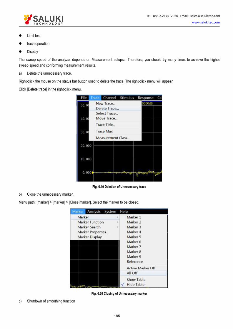
Tel: 886.2.2175 2930 Email: [email protected]
www.salukitec.com
185
Limit test
trace operation
Display
The sweep speed of the analyzer depends on Measurement setupss. Therefore, you should try many times to achieve the highestsweep speed and conforming measurement results.
a) Delete the unnecessary trace.
Right-click the mouse on the status bar button used to delete the trace. The right-click menu will appear.
Click [Delete trace] in the right-click menu.
Fig. 6.19 Deletion of Unnecessary trace
b) Close the unnecessary marker.
Menu path: [marker] > [marker] > [Close marker]. Select the marker to be closed.
Fig. 6.20 Closing of Unnecessary marker
c) Shutdown of smoothing function

Tel: 886.2.2175 2930 Email: [email protected]
www.salukitec.com
186
Menu path: [Response] > [Average] > [Smooth...]. The [Smooth] dialog box will appear.
Click [Smooth ON/off] to shut down the smoothing function.
Fig. 6.21 Shutdown of Smoothing Function
d) Shutdown of limit test
Menu path: [Analysis] > [Limit test...]. The [Limit test] dialog box will appear. Click [Limit test ON/off] check box to shut down the limittest function.
Fig. 6.22 Shutdown of Limit Test
e) Shutdown of trace operation function
Menu path: [Analysis] > [Memory] > [Save/ Operate]. Select the data in the [trace statistic] box.
Tel: 886.2.2175 2930 Email: [email protected]
www.salukitec.com
187
Fig. 6.23 Shutdown of trace Operation Function
6.10. Improvement of Efficiency of Multi-state Measurement
If multiple parameter measurements are required to represent the characteristics of one device, various methods can be applied toimprove the measurement efficiency. You can try the following methods to find the most suitable application solution.
Improvement of measurement efficiency by Measurement setups
Automatic change of Measurement setups
Rapid calling of measurement
6.10.1. Improvement of Measurement Efficiency by Measurement setupsIn order to improve the measurement efficiency of the tested device requiring various parameter measurements, you should be familiarwith the analyzer operation, which can help to create the optimal application solution. See trace, channel and window details related toparameter measurements in “3.4 trace, Channel and Window of Analyzer".
1) Reasonably arrange one group of measurements.
Arrange one group of measurements of the tested device in one instrument state. Save the instrument state so as to perform theprevious group of measurements by calling. Or, arrange a group of measurements by the preconfigured Measurement setups functionof the analyzer. See details in “Setting of preconfigured measurement" of “4.8 Observation of multiple tracks and opening of multiplechannels".
2) Apply the segment sweep function.
Segment sweep can be applied to change the following settings to represent multiple parameter measurements of one device.
Frequency range
power level
IF bandwidth
Number of scanning point
A group of frequency ranges with respective attributes can be defined in segment sweep. In this case, the tested device with multipleMeasurement setupss can be measured by means of one sweep. See segment sweep details in the “Setting of segment sweep type"of “4.5.2 Setting of sweep type" of “4.5 Setting of sweep".
3) Selectively trigger the measurement.
Set the measurement as follows by triggering.
Continuously update the measurement with rapid data changes.
Occasionally update the measurement with a few data changes.
For example, the tuning measurement of one filter can be set by the following settings:
One channel is used to measure the passband response of the filter in tuning.
One channel is used to measure the out-of-band response of the filter.
In this case, the turning measurement of the filter can be observed continuously. If all channels are updated constantly, the responsespeed of the analyzer will be reduced, and the filter cannot be tuned rapidly. Measurement setups is introduced as follows.
Measurement data of Channel 1 will be updated continuously.
Measurement data of Channel 2 will be updated when required.
a) Use the mouse.

Tel: 886.2.2175 2930 Email: [email protected]
www.salukitec.com
188
1. Create the double-channel measurement.Menu path: [Response] > [Display] > [Measurement setups] > [Setting D].
2. Set the trigger mode of Channel 1: constantly update measurement data.Menu path: [Stimulus] > [Trigger] > [Trigger...]. The [Trigger] dialog box will appear. Select the [Internal] radio box in the trigger sourcezone.
Click the [Channel] box in the trigger setting zone and select Channel 1. Click the [Constantly] radio box in the trigger setting zone.
3. Click the [Channel] box in the trigger setting zone and select Channel 2.Set the trigger mode of Channel 2: update measurement data when required.
Click the [Once] or [Group] radio box in the trigger setting zone. If the group triggering mode is selected, enter the group number in the[Group] input box.
4. Click [Soft keyboard] in the [System] menu.The [Soft keyboard] dialog box will appear. Click [Stimulus] > [Trigger] in the dialogbox and the toolbar to trigger the corresponding soft key will appear.
5. Click the window below to set Channel 2 as the current active channel.6. Update the measurement data of Channel 2.7. Click the [Once], [Group sweep] or [Re-sweep] on the trigger soft key toolbar. Measurement data of Channel 2 will be updated.
6.10.2. Automatic Change of Measurement setups
Automatically change Measurement setupss by means of programming to effectively improve the efficiency of multi-parametermeasurements.
6.10.3. Rapid calling of measurement
The most effective method to call the measurement is to save a group of measurements as one instrument state.
The time difference of calling the instrument with one or more measurements is little.
The corresponding time is required in each calling. The calling time can be saved by setting a group of measurements.
6.11. Rapid Data TransmissionRapid data transmission can help to improve the measurement efficiency. You can apply the following methods to increase the datatransmission speed.
Rapid calling of measurement
Minimization of transmission data
Use of real number format
Use of LAN
Use of COM program
6.11.1. Use of “Single” Trigger Mode
Use the "single" trigger mode to complete measurement before data transmission. Menu path: [Stimulus] > [Trigger] > [Trigger...]. The[Trigger] dialog box will appear. Select the [Internal] radio box in the trigger source zone.
Select the measurement channel for data transmission by clicking the [Channel] box in the trigger setting zone. Click the [Constantly]radio box in the trigger setting zone and then click [OK] to close the dialog box.
Update the measurement results:

Tel: 886.2.2175 2930 Email: [email protected]
www.salukitec.com
189
1) Click the corresponding trace state button to set the trace and channel to be updated as the active trace and channel.
2) Click [Soft keyboard] in the [System] sub-menu. Then click [Stimulus] > [Trigger] in the [Soft keyboard] dialog box.
3) Click [Once] in the trigger soft key toolbar.
6.11.2. Minimization of Transmission Data
Apply the segment scanning function to reduce the number of trace points, instead of transmission of the whole trace with a lot oflinear points.
6.11.3. Use of Real Number Format
Select the real number format in automatic measurement using SCPI so as to achieve the highest transmission speed.
6.11.4. Use of LAN
Use the LAN to increase the data transmission speed in the automatic SCPI measurement application.
6.11.5. Use of COM ProgramUse COM in the automatic measurement program to achieve the highest speed of data transmission.
6.12. Use of Macro
The macro is an executable file installed and run in the analyzer. S3602 series vector network analyzers support up to 10 macros.
New macro
[Macro setting] dialog box
[Macro setting window] dialog box
6.12.1. New macro
Menu path: [System] > [Macro] > [Macro setting...]. The [Macro setting] dialog box will appear.
Fig. 6.24 Macro Setting
Click the [Macro setting] dialog box to activate the blank line under the macro settings. Click the [Edit...] button and the [Macro settingwindow] dialog box will appear.
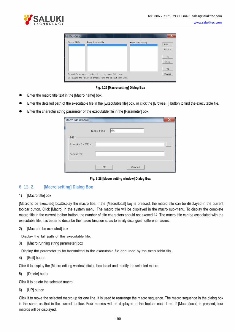
Tel: 886.2.2175 2930 Email: [email protected]
www.salukitec.com
190
Fig. 6.25 [Macro setting] Dialog Box
Enter the macro title text in the [Macro name] box.
Enter the detailed path of the executable file in the [Executable file] box, or click the [Browse...] button to find the executable file.
Enter the character string parameter of the executable file in the [Parameter] box.
Fig. 6.26 [Macro setting window] Dialog Box
6.12.2. [Macro setting] Dialog Box
1) [Macro title] box
[Macro to be executed] boxDisplay the macro title. If the [Macro/local] key is pressed, the macro title can be displayed in the currenttoolbar button. Click [Macro] in the system menu. The macro title will be displayed in the macro sub-menu. To display the completemacro title in the current toolbar button, the number of title characters should not exceed 14. The macro title can be associated with theexecutable file. It is better to describe the macro function so as to easily distinguish different macros.
2) [Macro to be executed] box
Display the full path of the executable file.
3) [Macro running string parameter] box
Display the parameter to be transmitted to the executable file and used by the executable file.
4) [Edit] button
Click it to display the [Macro editing window] dialog box to set and modify the selected macro.
5) [Delete] button
Click it to delete the selected macro.
6) [UP] button
Click it to move the selected macro up for one line. It is used to rearrange the macro sequence. The macro sequence in the dialog boxis the same as that in the current toolbar. Four macros will be displayed in the toolbar each time. If [Macro/local] is pressed, fourmacros will be displayed.

Tel: 886.2.2175 2930 Email: [email protected]
www.salukitec.com
191
7) [DOWN] button
Click it to move the selected macro down for one line.
6.12.3. [Macro setting window] dialog box1) [Macro name] box
Set the macro title name.
2) Editing zone
a) [Executable file] box
Set the full path of the executable file.
b) [Browse...] button
Browse the drive and director, position the executable file and establish the full path of the executable file.
c) [Parameter] box
Used to set the character string parameter to be transmitted to the executable file for reference.

Tel: 886.2.2175 2930 Email: [email protected]
www.salukitec.com
192
7. CalibrationCalibration can help to reduce the measurement error. This chapter includes the following contents:
Calibration overview
Selection of calibration type
Calibration guide
High-accuracy measurement calibration
Measurement error
Editing of calibration kit definition
Calibration standards
TRL calibration
Fixture compensation calibration
Electronic calibration
7.1.Calibration OverviewMeasurement calibration is a process to determine the system errors according to the standards of the existing measurementcharacteristics and then eliminate the influence of system errors during measurement of the tested device. It can help to reduce themeasurement error and improve the measurement accuracy of the analyzer.
7.1.1. Definition of Calibration
Calibration is a process to eliminate one or more system error(s) with the error model. The error item of the error model is solved bymeasurement according to high-quality calibration standards (including the open-circuit device, short-circuit device, load and throughtype part). See system error details in "7.5.3 System Error" of "7.5 Measurement Error" in this chapter.
Select the appropriate calibration method according to the measurement type and accuracy requirements. See details in "7.2Selection of Calibration Type".
Various kinds of calibration can be done according to the calibration guide of the calibration. See details in "7.3 Calibration Guide".
The measurement accuracy after calibration depends on the quality of the calibration standard and the model definition accuracy ofthe standard calibration kit in the calibration kit definition file. The calibration kit definition file is saved in the analyzer. In order toensure the measurement accuracy, the actual calibration kit must conform to the requirements of the calibration kit definition file. Seeaccurate calibration details in "7.4 High- accuracy Measurement Calibration".
The user must correctly define the calibration standard in the calibration kit definition file of the user so as to use the customcalibration kit (e.g. for fixture measurement calibration). See details in "7.6 Editing of Calibration Kit Definition".
7.1.2. Significance of CalibrationIt is impossible to make an ideal analyzer requiring no error correction from the perspective of hardware circuit. Even if error correctioncan be ignored in good hardware circuits, the costs will be high. In addition, the measurement accuracy of the analyzer is largelyinfluenced by external accessories. The amplitude and phase changes of test components such as the connecting cable and adapterwill affect response the real response of the tested device. Therefore, the best method is to balance the hardware performance andcost, make high-quality hardware as practical as possible and improve the measurement accuracy by calibration.
7.1.3. Applications of Calibration
High measurement accuracy is expected.

Tel: 886.2.2175 2930 Email: [email protected]
www.salukitec.com
193
Different types of connector or impedance are used.
A cable is connected between the tested device and the test port of the analyzer.
The tested device is measured in a wide frequency range or a device of long electrical delay is measured.
An attenuator or similar device is connected to the input or output end of the tested device.
7.1.4. Simple Calibration Process1) Connect the analyzer according to the measurement requirements.
2) Select the appropriate analyzer to optimize measurement.
3) Remove the tested device and select the calibration type and kit according to the calibration guide.
4) Connect the standard calibration kit of the selected type in measurement according to the calibration guide. The error iscalculated by measurement with the standard calibration kit and saved in the memory of the analyzer.
5) Reconnect and measure the tested device. If error correction is applied during measurement, the error influence will beeliminated.
7.2.Selection of Calibration Type
S3602 series vector network analyzers support six common calibration types, with details as follows:
1) Open-circuit response
a) Calibration accuracy: low to medium.
b) Measurement parameter: S11, S22, S33 and S44.
c) Standard calibration kit: open-circuit device.
d) System error correction: reflection tracking.
e) Measurement application: reflection measurement of any port.
2) Short-circuit response
a) Calibration accuracy: low to medium.
b) Measurement parameter: S11, S22, S33 and S44.
c) Standard calibration kit: short-circuit device.
d) System error correction: reflection tracking.
e) Measurement application: reflection measurement of any port.
3) Through type response
a) Calibration accuracy: medium.
b) Measurement parameter: S-parameter of transmission measurement.
c) Standard calibration kit: through type device.
d) System error correction: transmission tracking.
e) Measurement transmission measurement in any direction.
The adapter is used as the through type device.

Tel: 886.2.2175 2930 Email: [email protected]
www.salukitec.com
194
The through type device is of zero length and loss according to the definition in the calibration kit definition file. If the adapter is usedas the through type device in calibration, the characteristics of the adapter must be specified in the calibration kit definition file toensure the accuracy of calibration. See details in "7.4 High-accuracy Measurement Calibration".
4) Through type response and isolation
a) Calibration accuracy: medium.
b) Measurement parameter: S-parameter of transmission measurement.
c) Standard calibration kit: through type device and two load (one respectively for each port).
d) System error correction:
Transmission tracking
Crosstalk
e) Measurement application:
Transmission measurement in any direction.
Improvement of the dynamic range of the system by means of isolation calibration.
Isolation calibration
Isolation calibration is not allowed if all the ports are not respectively connected with one load at the same time.
5) One-port (reflection)
a) Calibration accuracy: high
b) Measurement parameter: S11, S22, S33 and S44.
c) Standard calibration kit: open-circuit device, short-circuit device and load.
d) System error correction:
Direction
Source matching
Reflection tracking
e) Measurement application: reflection measurement of any port.
6) Full 2-port SOLT
a) Calibration accuracy: high
b) Measurement parameters: all
c) Standard calibration kit: open-circuit device, short-circuit device, load and through type device.
d) System error correction:
Direction
Source matching
Reflection tracking
Crosstalk
Transmission tracking
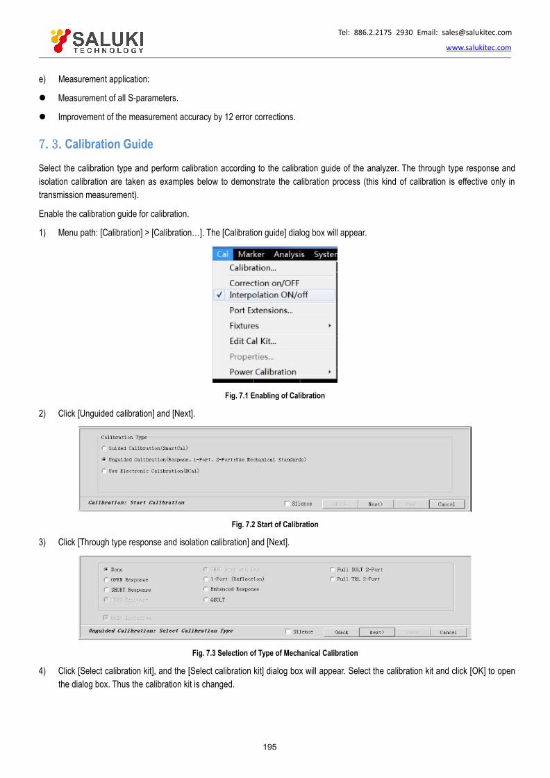
Tel: 886.2.2175 2930 Email: [email protected]
www.salukitec.com
195
e) Measurement application:
Measurement of all S-parameters.
Improvement of the measurement accuracy by 12 error corrections.
7.3.Calibration Guide
Select the calibration type and perform calibration according to the calibration guide of the analyzer. The through type response andisolation calibration are taken as examples below to demonstrate the calibration process (this kind of calibration is effective only intransmission measurement).
Enable the calibration guide for calibration.
1) Menu path: [Calibration] > [Calibration…]. The [Calibration guide] dialog box will appear.
Fig. 7.1 Enabling of Calibration
2) Click [Unguided calibration] and [Next].
Fig. 7.2 Start of Calibration
3) Click [Through type response and isolation calibration] and [Next].
Fig. 7.3 Selection of Type of Mechanical Calibration
4) Click [Select calibration kit], and the [Select calibration kit] dialog box will appear. Select the calibration kit and click [OK] to openthe dialog box. Thus the calibration kit is changed.
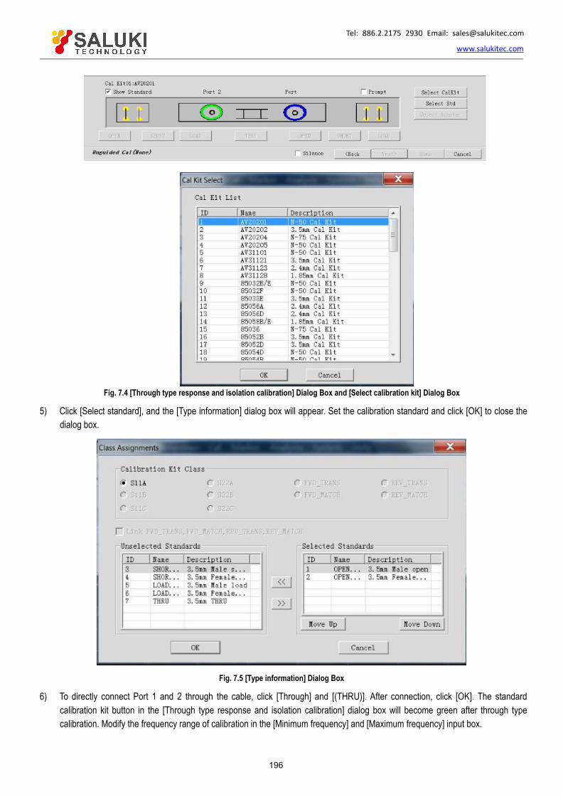
Tel: 886.2.2175 2930 Email: [email protected]
www.salukitec.com
196
Fig. 7.4 [Through type response and isolation calibration] Dialog Box and [Select calibration kit] Dialog Box
5) Click [Select standard], and the [Type information] dialog box will appear. Set the calibration standard and click [OK] to close thedialog box.
Fig. 7.5 [Type information] Dialog Box
6) To directly connect Port 1 and 2 through the cable, click [Through] and [(THRU)]. After connection, click [OK]. The standardcalibration kit button in the [Through type response and isolation calibration] dialog box will become green after through typecalibration. Modify the frequency range of calibration in the [Minimum frequency] and [Maximum frequency] input box.

Tel: 886.2.2175 2930 Email: [email protected]
www.salukitec.com
197
Fig. 7.6 [Measurement of multiple standard kits] Dialog Box
7) Respectively connect Port 1 and 2 to the load calibration kit. Click [Load] and the keys of the standard kit type and interface type(the display contents vary from calibration types). After selection, click [OK]. Modify the frequency range of calibration in the[Minimum frequency] and [Maximum frequency] input box. The standard calibration kit button in the [Through type response andisolation calibration] dialog box will become green after isolation calibration.
Fig. 7.7 [Measurement of multiple standard kits] Dialog Box
8) Click [OK] in the [Through type response and isolation calibration] dialog box after calibration.
Fig. 7.8 [Through type response and isolation calibration] Dialog Box
Notes:
1. The optional calibration type is associated with the measurement parameters of the current active channel. For example, if themeasurement parameter is S11, the through type response mode or the through type response and isolation calibration modecannot be selected.
2. If isolation calibration is not required in the full 2-port calibration, tick the [Ignore isolation (2-port type)] check box.
Properly select the calibration standard to realize the highest calibration accuracy.
The [Measurement of multiple standard kits] dialog box shows the standard connector types, instead of the connector types fornon-test ports. In order to realize the highest calibration accuracy, the calibration standard must be selected properly.

Tel: 886.2.2175 2930 Email: [email protected]
www.salukitec.com
198
7.4.High-accuracy Measurement Calibration
The calibration accuracy depends on the selected calibration type, calibration kit quality and calibration process. This section mainlydiscusses how to perform high-accuracy calibration.
1) Measurement reference plane
The tested device is not directly connected to the port of the analyzer in most of measurements. Instead, it is connected through thetest fixture or cable. The connection point of the tested device must be calibrated to realize the highest measurement accuracy. Thispoint is called the measurement reference plane. If the measurement reference plane is calibrated, the error related to themeasurement composition (such as the cable, test fixture and adapter between the analyzer port and reference plane) can bemeasured and eliminated.
2) Influence of calibration kit
Under normal conditions, the calibration standard of the calibration kit is the same as the connector type standard of the tested device.In some cases, however, the calibration kit corresponding to the connector type of the tested device is not provided. For example, theport size of the tested device is 2.4mm, but the connector size of the analyzer and calibration kit is 3.5mm. If the 2.4mm calibration kitis used for calibration and the 2.4mm/3.5mm adapter is used in measurement, the measurement error will be obvious, especially inreflection measurement, as the adapter is not calibrated. If the applied calibration kit is different from the calibration kit specified forcalibration, the calibration accuracy will be reduced. The degree of accuracy reduction depends on the difference between thespecified calibration kit and actual calibration kit.
3) Accuracy of interpolation measurement
If the instrument settings are different from calibration settings, calibration data can be automatically interpolated into the analyzer. Inthis case, the measurement accuracy cannot be predicted and may drop greatly or not be affected. The measurement error must bedetermined depending on the actual situation. If the phase shift added by two measurement points exceeds 180 degrees, themeasurement accuracy will drop greatly as the correct phase data cannot be interpolated. Generally, the probability of accuracyreduction may increase as a result of interpolation in the following cases:
When the frequency span between measurement points is increased;
When the frequency span between measurement points is too large;
When the measurement frequency is high, especially above 10GHz.
4) Influence of power level
The power level must not be changed after calibration in order to realize the highest accuracy of error correction. However, if thepower level is changed under the same conditions as the attenuator settings in calibration, the accuracy of S-parameter measurementonly declines a little. If the attenuator settings are changed, the accuracy of error correction will decline further.
5) System impedance
The system impedance must be changed in measurement of the impedance device (not 50Ω) such as the waveguide device. Thedefault system impedance is 50Ω.
a) Setting of system impedance
Menu path: [System] > [Configuration] > [System impedance...].
Enter the system impedance value in the [Impedance] box and click [OK] to close the dialog box.
6) Port extension
The measurement reference plane may be changed as a result of connection of the cable, adapter or fixture after calibration, whichmay lead to increase of the phase shift. In this case, the additional phase offset can be compensated by means of port extension. Portextension is the simplest method to compensate the additional phase shift between the calibration plane and tested device plane, butcannot be used to compensate the loss and mismatch of the path between the calibration plane and tested device plane. Therefore,

Tel: 886.2.2175 2930 Email: [email protected]
www.salukitec.com
199
the loss and mismatch should be minimized to realize the highest measurement accuracy. For setting of port extension, refer to"Setting of port extension" in "6.5 Improvement of Phase Measurement Accuracy".
7) Correct isolation calibration
Isolation calibration in full 2-port calibration is applied to correct the crosstalk error between ports. It is required only in measurementof large insertion loss, such as the out-of-band suppression of the filter, isolation of the switch, etc. When the crosstalk signal is closeto the base noise of the analyzer, additional noise will be produced in the error model as a result of isolation calibration. In order toimprove the calibration accuracy, you should:
Perform isolation calibration if necessary;
Use the narrow IF bandwidth;
Reduce noise by sweep averaging.
The test port of the analyzer should be connected with a load in isolation calibration. In order to realize the highest calibrationaccuracy, it is preferred to connect the loads to two measurement ports at the same time for isolation calibration. If only one load isprovided, connect a well-fitted device to the non-measurement port.
7.5.Measurement Errors
Understanding of the source of measurement error and the way of error correction can help to improve the measurement accuracy, asa certain degree of uncertainty still exits no matter how carefully the measurement is done. The following kinds of errors may beproduced in measurement with the analyzer.
7.5.1. Drift Errors Drift errors are produced by performance changes of the instrument or test system after calibration.
The thermal expansion of the interconnected cables in the instrument and the performance changes of microwave mixer aremain causes of the drift error. The drift errors can be eliminated by recalibration.
The duration of accurate calibration depends on the test environment. The stable environment can help to minimize the drifterror.
7.5.2. Random ErrorsThe random error cannot be predicted or eliminated by means of calibration. The influence on measurement results can be reducedby some methods. Random errors are mainly divided into three types:
1) Random error of instrument
a) Electrical disturbance of internal components of the analyzer may result in random noise, mainly including:
Low-level noise arising from the base noise within the receiver broadband;
High-level noise or data trace jittering, which is mainly caused by the base noise inside the instrument and phase noise of the LOsource.
b) The random noise error can be reduced in the following methods:
Increase the source power input into the tested device;
Reduce the IF bandwidth;
Apply the function of sweep averaging.
2) Switch repeatability error
The switch is used to change attenuator settings of the source. If the switch acts, contact closing may be different from previousclosing sometimes. In this case, the measurement accuracy will be affected seriously. Therefore, the attenuator settings should not be

Tel: 886.2.2175 2930 Email: [email protected]
www.salukitec.com
200
changed in high-accuracy measurement so as to reduce the switch repeatability error.
3) Connector repeatability error
Connector wear may result in electrical performance changes. Proper connection maintenance can help to reduce the connectorrepeatability error.
7.5.3. System ErrorsSystem errors are caused by non-ideal hardware properties and may be repeatable (therefore, it can be predicted). It is assumed thatsystem errors do not change over time. System errors can be determined by calibration and eliminated by mathematical calculation inmeasurement.
System errors cannot be fully eliminated. Due to limitations of the calibration process, some residual errors may exist after calibration,mainly resulting from:
Non-ideal calibration standard;
Connector connection;
Interconnected cable;
Instrument.
All measurements are affected by the dynamic accuracy and frequency errors. For reflection measurement, relevant residual errorsinclude:
Effective direction;
Effective source matching;
Effective reflection tracking.
For transmission measurement, relevant residual errors include:
Crosstalk
Effective load matching;
Effective transmission measurement.
1) Direction errors
The directional coupler or bridge is used for reflection measurement. The coupling end of the ideal coupler can only output thereflection signal to the receiver for measurement. Actually, a small number of incident signals will leak to the coupling port through themain channel of the coupler, which may result in directional errors in measurement. Directional errors can be determined and reducedin the following methods.
Connect the load to the measurement port during calibration and regard the load port free from reflection.
The output signal of the coupling port is the leakage error signal.
Reduce the directional error signals in reflection measurement.
2) Crosstalk errors
Ideally, only the transmission signal through the tested device can reach the receiver. Actually, a small number of signals reach thereceiver through other paths in the analyzer. Such signals are called crosstalk signals. Crosstalk errors can be determined andreduced in the following methods.
Connect the loads to Port 1 and 2 at the same time during calibration.
The signal measured by the measurement receiver is the leakage signal of the analyzer.
Eliminate the crosstalk errors by means of error correction during transmission measurement.

Tel: 886.2.2175 2930 Email: [email protected]
www.salukitec.com
201
3) Source matching errors
Ideally, the measurement receiver can receive all signals reflected from the tested device in reflection measurement. Actually, part ofthe signals reflected by the tested device are reflected by the measurement port back to the tested device. As such signals cannot bemeasured by the measurement receiver, source matching errors will be produced. They can be determined and reduced in thefollowing methods.
Connect the short-circuit device to the measurement port in calibration. The signals reflected by the short- circuit device will bemeasured by the receiver. Measurement results will be saved in the analyzer.
Connect the open-circuit device to the port. The signals reflected by the open-circuit device will be measured by the receiver.Measurement results will be saved in the analyzer.
The measurement results will be compared with the known values of the open-circuit device and short-circuit device todetermine source matching errors.
Eliminate source matching errors by means of error correction in reflection and transmission measurement.
4) Load matching errors
In the ideal transmission measurement, transmission signals through the tested device are received by the measurement receiver.Actually, part of the signals are reflected by the test port and cannot be measured, thus resulting in load matching errors. The loadmatching errors can be determined and reduced in the following methods.
Directly connect Port 1 and 2, with zero length.
If the source is located on Port 1, measurement signals of Receiver A includes the reflection signals of Port 2. If the source islocated on Port 2, measurement signals of Receiver 2 include the reflection signals of Port 2. Thus, load matching errors can bedetermined.
Eliminate source matching errors by means of error correction in reflection and transmission measurement.
5) Reflection tracking errors
The signals of Receiver A and R1 or B and R2 are compared in reflection measurement. This is called ratio measurement. In the idealreflection measurement, the frequency responses of Receiver A and R1 or B and R2 should be identical. Actually, this is impossibleand reflection tracking errors may be produced, i.e. vector sum errors caused by test deviations. The error amplitude and phasechange with the frequency. Deviations are mainly caused by the following factors:
Signal separator;
Test cable and adapter;
Difference between the reference and test signal paths.
Reflection tracking errors can be determined and reduced in the following methods.
Connect the short-circuit device to the measurement port in calibration. The signals reflected by the short- circuit device will bemeasured by the receiver. Measurement results will be saved in the analyzer.
Connect the open-circuit device to the port. The signals reflected by the open-circuit device will be measured by the receiver.Measurement results will be saved in the analyzer.
The measurement results will be compared with the known values of the open-circuit device and short-circuit device todetermine source matching errors.
Eliminate reflection tracking errors by means of error correction in reflection and transmission measurement.
6) Transmission tracking errors
The signals of Receiver A and R2 or B and R1 are compared in transmission measurement. This is called ratio measurement. In theideal transmission measurement, the frequency responses of Receiver A and R2 or B and R1 should be identical. Actually, this isimpossible and transmission tracking errors may be produced, i.e. vector sum errors caused by test deviations. The error amplitude

Tel: 886.2.2175 2930 Email: [email protected]
www.salukitec.com
202
and phase change with the frequency. Deviations are mainly caused by the following factors:
Signal separator;
Test cable and adapter;
Difference between the reference and test signal paths.
Transmission tracking errors can be determined and reduced in the following methods.
Directly connect Port 1 and 2, with zero length.
Measure the signals of Receiver A and R2 or B and R1.
Determine transmission tracking errors by comparing the signals of two receivers.
Eliminate transmission tracking errors by means of error correction in transmission measurement.
7.6.Editing of Calibration Kit Definition
The [Edit calibration kit] dialog box is used to edit the definition of the calibration kit or create a user-defined calibration kit.
Calibration kit definition
Custom calibration kit
Create calibration kit
Edit calibration kit
[Edit calibration kit] dialog box
[Add connector] dialog box
[Type information] dialog box
[Add standard] dialog box
[Open-circuit device] dialog box
[Short-circuit device] dialog box
[Load] dialog box
[Through type/transmission line/adapter] dialog box
7.6.1. Calibration Kit DefinitionEach standard calibration kit (represented by the standard kit ID) is a specific and accurately defined physical device. For example,ID1 of 85056A calibration kit means a 2.4mm male open-circuit device. Standard kits are divided into four types: open-circuit device,short-circuit device, load and through type device/adapter/air line. Each type of calibration kit is has the specific model structure,including the number and physical characteristics of the standard kit. The majority of calibration kits are equipped with a group ofadapters subject to accurate phase matching. The other standard calibration kits must be defined before use.
7.6.2. Custom Calibration KitSometimes you may need to edit the calibration kit definition file or create the user-defined calibration kit. In most of measurementapplications, the default calibration kit model is suitable for accurate calibration. However, the user-defined calibration kit should becreated in the following applications.
The connector type is different from that defined in the calibration kit model.
The standard calibration kit different from the defined is used. For example, use three short-circuit devices of different deviationsinstead of the open-circuit device, short-circuit device and load in one-port calibration.

Tel: 886.2.2175 2930 Email: [email protected]
www.salukitec.com
203
Improve the accuracy of the predefined calibration kit model. If the actual properties of the standard calibration kit can bedescribed with the model, the calibration will be more accurate. For example, change the load impedance into 50.1Ω, instead ofthe defined 50Ω.
To create the user-defined calibration kit, first define the connector type, such as APC7, 3.5mm, APC2.4mm (50Ω), etc. Although morethan one connector type can be defined, it is preferred to define one connector type for each kind of calibration kit. The female andmale connectors must be defined separately.
7.6.3. Create Calibration Kit1) Click [Calibration] > [Edit calibration kit...]. The [Edit calibration kit] dialog box will appear.
2) Click [Insert new calibration kit]. The [Edit calibration kit] dialog box will appear.
a) Input the name of the user-defined calibration kit in the [Calibration kit name] box.
b) Click [Add] in the connector type zone. The [Add connector] dialog box will appear.
3) In the [Add connector] dialog box:
a) Enter the connector name in the name box.
b) Select the connector type of the calibration kit in the connector type zone: [Female], [Male] or [No Gender].
c) Set the minimum and maximum working frequency range of the connector in the frequency range zone.
d) Enter the characteristic impedance (such as 50Ω) of the connector in the impedance zone [Z0].
e) Select the connector medium type in the [Medium] box: coaxial or waveguide.
f) Check the entered contents and click [OK] to close the dialog box. Then it is not allowed to edit connector information.
g) The connector of the other polarity can be added by click [Add] in the connector type zone of the [Edit calibration kit] dialogbox and repeated the above steps.
3. Click [Add] under the [Standard kit] box of the [Edit calibration kit] dialog box. The [Add standard kit] dialog box will appear.Select the standard kit to be added: [Open-circuit device], [Short-circuit device], [Load], [Through type], [Adapter] and[Transmission line]. Click [OK] to close the [Add standard kit] dialog box. At the same time, the [Edit] dialog box corresponding tothe selected standard kit will appear.
4. In the [Standard] (such as open-circuit device) dialog box, enter the definition data. For the limited standard kit, the frequencyrange may be different from that of the connector. Set the frequency range according to the actual minimum and maximumfrequency of the standard kit, and click [OK] to close the dialog box.
5. Repeat Step 4) and 5) to define all standard calibration kits among custom calibration kits.
7.6.4. Edit calibration kit1. Click [Calibration] > [Edit calibration kit...]. The [Edit calibration kit] dialog box will appear.2. Click the calibration kit to be modified in the dialog box.3. Click [Edit calibration kit]. The [Edit calibration kit] dialog box will appear. Edit the calibration kit.4. [Open] buttonOpen the calibration kit list and calibration kit definition file.
5. [Save as] buttonSave the current calibration kit list and calibration kit definition as a file.
6. [Restore all calibration kits] buttonReinstall all calibration kits supported by the network analyzer.
7. Calibration kit installation zonea) [Import calibration kit] button

Tel: 886.2.2175 2930 Email: [email protected]
www.salukitec.com
204
Call the [Open] dialog box and import the calibration kit definition in the hard disc or other drives.
b) [Save as] button
Open the [Save as] dialog box to save the selected calibration kit definition.
c) [Insert new calibration kit] button
Open the [Edit calibration kit] dialog box to create a new calibration kit definition.
d) [Edit calibration kit] button
Open the [Edit calibration kit] dialog box and modify the selected calibration kit definition.
e) [Delete calibration kit] button
Delete the selected calibration kit definition.
f) [Recover calibration kit] button
Recover the modification of the selected calibration kit into the factor setting state.
g) [∧] and [∨] button
Click the [∧] and [∨] button to select the calibration kit.
7.6.5. [Edit calibration kit] Dialog Box
Fig. 7.10 [Edit calibration kit] Dialog Box
1) Calibration kit identification zone
a) [Calibration kit ID] box
Display or edit the ID number of the existing calibration kit (or the inserted new calibration kit).
b) [Calibration kit name] box
Display or edit the name of the calibration kit.
c) [Calibration kit description] box

Tel: 886.2.2175 2930 Email: [email protected]
www.salukitec.com
205
Display or edit the characteristic description of the calibration kit.
2) Connector type zone
a) [Connector] box
Click the [Connector] box or arrow button to select the connector type.
b) [Add] button
Click the [Add] button. The [Add connector] dialog box will appear. Add the new connector type of the calibration kit.
c) [Modify] button
The [Modify connector name] dialog box will appear. Modify the connector name.
Fig. 7.11 [Change connector name] Dialog Box
3) Type zone
a) [Calibration method] box
Click it to select the calibration method corresponding to the type.
b) [Edit type] button
Click it and the [Type information] dialog box to set the type of the calibration kit.
4) Standard zone
a) [Calibration kit] box
Display the ID, name and description of the calibration kit supported by the analyzer at present.
b) [Add] button
The [Add standard] dialog box will appear. Add the new definition of calibration standard.
c) [Edit] button
Click it and the [Standard calibration kit (such as the open-circuit device, short-circuit device, load, through type connector/airline/adapter)] dialog box will appear. Modify the definition of the selected standard calibration kit.
d) [Delete] button
Delete the definition of the selected standard calibration kit.
e) [Delete all] button
Delete the definitions of all standard calibration kits.
f) [∧] and [∨] button
Select the standard calibration kit.
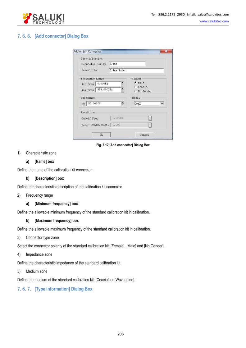
Tel: 886.2.2175 2930 Email: [email protected]
www.salukitec.com
206
7.6.6. [Add connector] Dialog Box
Fig. 7.12 [Add connector] Dialog Box
1) Characteristic zone
a) [Name] box
Define the name of the calibration kit connector.
b) [Description] box
Define the characteristic description of the calibration kit connector.
2) Frequency range
a) [Minimum frequency] box
Define the allowable minimum frequency of the standard calibration kit in calibration.
b) [Maximum frequency] box
Define the allowable maximum frequency of the standard calibration kit in calibration.
3) Connector type zone
Select the connector polarity of the standard calibration kit: [Female], [Male] and [No Gender].
4) Impedance zone
Define the characteristic impedance of the standard calibration kit.
5) Medium zone
Define the medium of the standard calibration kit: [Coaxial] or [Waveguide].
7.6.7. [Type information] Dialog Box

Tel: 886.2.2175 2930 Email: [email protected]
www.salukitec.com
207
Fig. 7.13 [Add connector] Dialog Box
1) Calibration kit type zone
Select the calibration type to be edited or observed.
2) [>>] and [<<] button
Click the [>>] and [<<] button to add or delete the standard calibration kit of the selected type or select the standard calibration kit inthe [Non-selected standard calibration kits] box. Click the [>>] button to add the selected standard calibration kit into the [Selectedstandard calibration kits] box. Select the standard calibration kit in the [Selected standard calibration kits] box. Click the [<<] button todelete the standard calibration kit of the selected type.
3) [∧] and [∨] button
Adjust the sequence of the standard calibration kits in the [Selected standard calibration kits] box. All the standard calibration kits inthe [Selected standard calibration kits] box will appear in the [Measurement of multiple standard kits] dialog box. Select thecorresponding standard calibration kit according to the polarity (female or male) of the measurement port and the frequency range ofthe measurement.
Select the standard calibration kit in the [Selected standard calibration kits] box. Click [∧] or [∨] to change the sequence of standardcalibration kits. This is usable in the following measurement applications. Multiple standard calibration kits are required for onecalibration type to cover the whole frequency range. The sequence of the standard calibration kits in the [Selected standard calibrationkits] box is the same as that in the [Measurement of multiple standard kits] dialog box.
7.6.8. [Add standard] Dialog Box
Fig. 7.14 [Add standard] Dialog Box
7.6.9. [Open-circuit device] Dialog Box
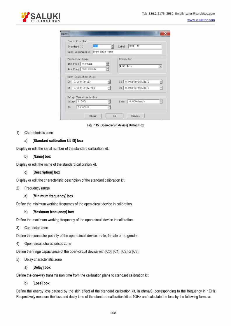
Tel: 886.2.2175 2930 Email: [email protected]
www.salukitec.com
208
Fig. 7.15 [Open-circuit device] Dialog Box
1) Characteristic zone
a) [Standard calibration kit ID] box
Display or edit the serial number of the standard calibration kit.
b) [Name] box
Display or edit the name of the standard calibration kit.
c) [Description] box
Display or edit the characteristic description of the standard calibration kit.
2) Frequency range
a) [Minimum frequency] box
Define the minimum working frequency of the open-circuit device in calibration.
b) [Maximum frequency] box
Define the maximum working frequency of the open-circuit device in calibration.
3) Connector zone
Define the connector polarity of the open-circuit device: male, female or no gender.
4) Open-circuit characteristic zone
Define the fringe capacitance of the open-circuit device with [C0], [C1], [C2] or [C3].
5) Delay characteristic zone
a) [Delay] box
Define the one-way transmission time from the calibration plane to standard calibration kit.
b) [Loss] box
Define the energy loss caused by the skin effect of the standard calibration kit, in ohms/S, corresponding to the frequency in 1GHz.Respectively measure the loss and delay time of the standard calibration kit at 1GHz and calculate the loss by the following formula:
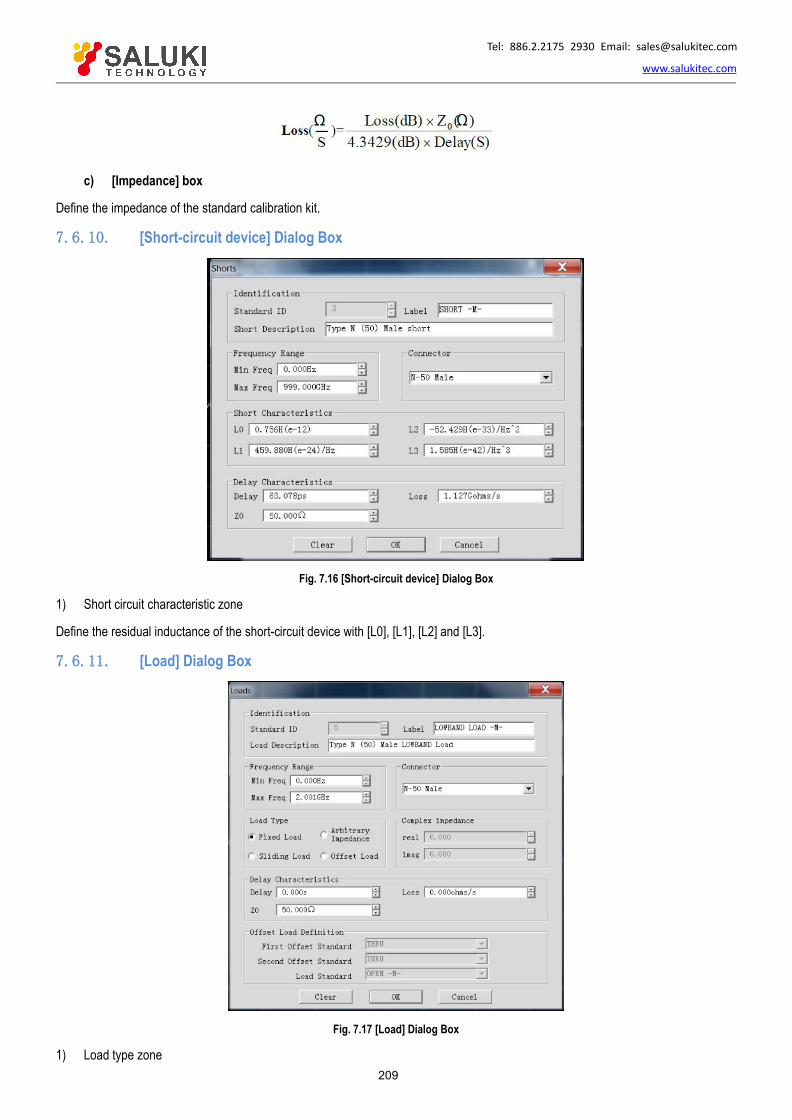
Tel: 886.2.2175 2930 Email: [email protected]
www.salukitec.com
209
c) [Impedance] box
Define the impedance of the standard calibration kit.
7.6.10. [Short-circuit device] Dialog Box
Fig. 7.16 [Short-circuit device] Dialog Box
1) Short circuit characteristic zone
Define the residual inductance of the short-circuit device with [L0], [L1], [L2] and [L3].
7.6.11. [Load] Dialog Box
Fig. 7.17 [Load] Dialog Box
1) Load type zone
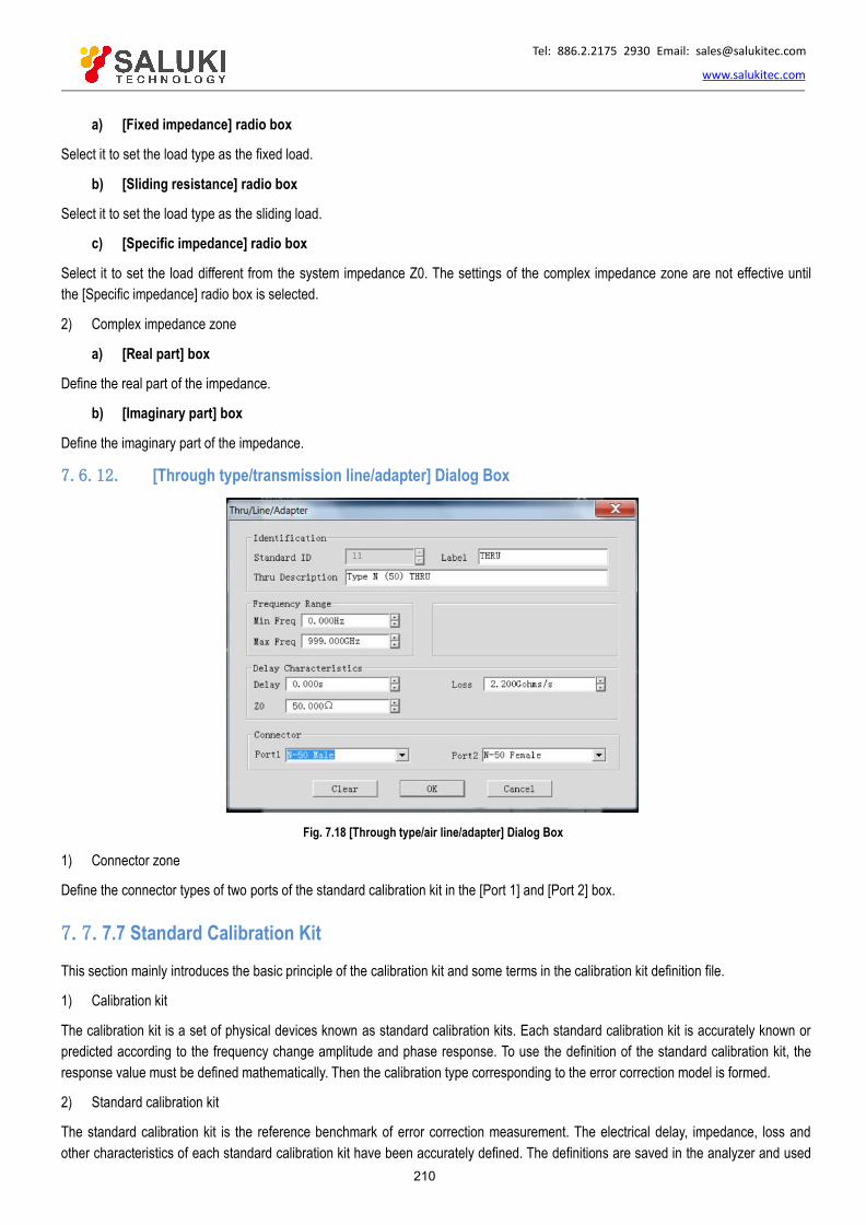
Tel: 886.2.2175 2930 Email: [email protected]
www.salukitec.com
210
a) [Fixed impedance] radio box
Select it to set the load type as the fixed load.
b) [Sliding resistance] radio box
Select it to set the load type as the sliding load.
c) [Specific impedance] radio box
Select it to set the load different from the system impedance Z0. The settings of the complex impedance zone are not effective untilthe [Specific impedance] radio box is selected.
2) Complex impedance zone
a) [Real part] box
Define the real part of the impedance.
b) [Imaginary part] box
Define the imaginary part of the impedance.
7.6.12. [Through type/transmission line/adapter] Dialog Box
Fig. 7.18 [Through type/air line/adapter] Dialog Box
1) Connector zone
Define the connector types of two ports of the standard calibration kit in the [Port 1] and [Port 2] box.
7.7.7.7 Standard Calibration Kit
This section mainly introduces the basic principle of the calibration kit and some terms in the calibration kit definition file.
1) Calibration kit
The calibration kit is a set of physical devices known as standard calibration kits. Each standard calibration kit is accurately known orpredicted according to the frequency change amplitude and phase response. To use the definition of the standard calibration kit, theresponse value must be defined mathematically. Then the calibration type corresponding to the error correction model is formed.
2) Standard calibration kit
The standard calibration kit is the reference benchmark of error correction measurement. The electrical delay, impedance, loss andother characteristics of each standard calibration kit have been accurately defined. The definitions are saved in the analyzer and used

Tel: 886.2.2175 2930 Email: [email protected]
www.salukitec.com
211
to calculate various errors of the error model. The analyzer can measure the responses of standard calibration kits in calibration, anderrors can be calculated by comparing the measurement results and the known values of the model. The influence of errors onmeasurement results is eliminated by mathematical operation which is also known as error correction.
3) Types of standard calibration kit
Four types of standard calibration kits are provided, corresponding to the structures or types of various definitions. The four types areas follows:
Standard calibration kit Terminal impedanceOpen-circuit device ∞ΩShort-circuit device 0Ω
Load System impedanceThrough type connector/air line/ adapter No terminal impedance
4) Definition of standard calibration kit
The definition of the standard calibration kit describes the electrical characteristics and frequency range, including:
a) Minimum frequency
Specify the allowable minimum frequency of the standard calibration kit in calibration.
b) Maximum frequency
Specify the allowable maximum frequency of the standard calibration kit in calibration.
c) Z0
Specify the characteristic impedance of the standard calibration kit, instead of the characteristic impedance of the system or theterminal impedance of the standard calibration kit.
d) Delay
Specify the uniform length of the transmission line between the defined standard calibration kit and actual calibration plane.
e) Type
Specify the type of the standard calibration kit: open-circuit device, short-circuit device, load and through type connector/airline/adapter.
f) Loss
Specify the energy loss caused by skin effects.
g) Definition of loss model
The loss unit is ohms/S, corresponding to the frequency unit 1GHz. Respectively measure the loss and delay time of the standardcalibration kit at 1GHz and calculate the loss by the following formula:
h) Fringe capacitance model of open-circuit device
The open-circuit device almost has no ideal reflection characteristics as a result of the effects of fringe capacitance at high frequency.The phase shift changes with the frequency. Such effects cannot be eliminated. The fringe capacitance is defined in the open-circuitdevice model. The capacitance model is a cubic polynomial function of the frequency. The polynomial coefficient is determinedaccording to the actual characteristics of the open-circuit device. The equation of the fringe capacitance model is as follows:
(F refers to the measurement frequency).

Tel: 886.2.2175 2930 Email: [email protected]
www.salukitec.com
212
i) Residual inductance model of short-circuit device
The short-circuit device almost has no ideal reflection characteristics as a result of the effects of residual inductance at high frequency.The phase shift changes with the frequency. Such effects cannot be eliminated. The fringe inductance is defined in the short-circuitdevice model. The inductance model is a cubic polynomial function of the frequency. The polynomial coefficient is determinedaccording to the actual characteristics of the open-circuit device. The equation of the residual inductance model is as follows:
(F refers to the measurement frequency).
7.8.TRL CalibrationTRL (Thru-Reflect-Line) calibration includes a series of calibration technologies, such as TRM (Thru-Reflect- Match). In the TRLcalibration, 12 error coefficients are determined with two standard calibration kits for transmission and one standard calibration kit forreflection. In the traditional SOLT calibration, however, 12 error coefficients are determined with one standard calibration kits fortransmission (T) and three standard calibration kits for reflection (SOL).
1) Why to perform TRL calibration?
TRL calibration is accurate and even more accurate than SOLT calibration in some cases. However, only a few calibration kits supportTRL. TRL calibration is always done when high measurement accuracy is required but the calibration kit of the same connector typeas the tested device is provided, such as use of the fixture in measurement or use of the probe in wafer measurement. In this case,the calibration kit with the same medium as the tested device must be created and defined. It is easier to make three TRL standardcalibration kits then to make four SOLT standard calibration kits. One disadvantage of TRL calibration is that multiple standardcalibration kits are required for the transmission line in broadband calibration. For example, two standard calibration kits are requiredfor the transmission line at 2GHz to 26GHz. The standard calibration kits for the transmission line should be particularly long at lowfrequency.
2) TRL standard calibration kit
Three standard calibration kits should be defined for TRL calibration: through type, reflection type and transmission type.
a) Through type standard calibration kit
The length of the through type can be zero or not zero. The zero-length through type is more accurate as a result of no loss orcharacteristic impedance. The electrical delay of the through type is different from that of the transmission type. The through typestandard calibration kit with the amplitude and phase defined accurately can be used to establish the measurement reference plane.
b) Reflection standard reflection kit
The reflection standard calibration kit is a physical device of large reflection coefficient. The reflection standard calibration kitsconnected to two measurement ports must have the same characteristics. If the reflection amplitude is not required but the phase isrequired in calibration, the electrical length of the standard calibration kit must be within 1/4 of the wavelength. The reflection standardcalibration kit with the amplitude and phase defined accurately can be used to establish the measurement reference plane.
c) Transmission line type standard calibration kit
The transmission line type standard calibration kit is used to measure the measurement reference impedance after calibration. TRLcalibration has the following disadvantages as a result of limitations of the transmission line type standard calibration kit.
The impedance of the transmission line type standard calibration kit must be the same as that of the through type standardcalibration kit.
The electrical length of the transmission line type standard calibration kit must be different from that of the through type standardcalibration kit.
The transmission line type standard calibration kit must have the appropriate electrical length within the whole frequency range.The phase difference of the transmission line type standard calibration kit and through type standard calibration kit must be

Tel: 886.2.2175 2930 Email: [email protected]
www.salukitec.com
213
between 20° and 160° at each frequency point. Therefore, the actual coverage range of a single transmission line is 8:1. In orderto cover a wider frequency range, multiple transmission line type standard calibration kits are required.
The transmission line type standard calibration kit should be particularly long at low frequency. The optimal length is 1/4 of thewavelength corresponding to the geometric average frequency (square root of the product of the starting frequency × endingfrequency) within the frequency span.
d) Matching standard calibration kit
If the transmission line of specific length or loss cannot be made, use the matching standard calibration kit instead of the transmissionline.
The matching standard calibration kit is a low-reflection terminal to be connected to the port.
Use the matching standard calibration kit as the transmission line of high loss and infinite length in calculation of the errorcoefficient of TRL calibration.
Change the impedance of the matching standard calibration kit into the reference impedance of measurement.
7.9.Fixture Compensation Calibration
The fixture simulator function is used for network port impedance conversion..., 2-port fixture de- embedding, Port Matching... andfour-port fixture embedding/de-embedding in the mathematical sense.
It can be used to simulate various measurements based on measurement results in applications, and also rapidly simulate thecorresponding measurement results in a real-time manner. The measurement results of the port with the impedance of 50Ω can betransformed into measurement results of any impedance by means of port impedance conversion.... The 2-port de-embeddingfunction can be applied to remove any network characteristic between the measurement end face and DUT end face, which is definedin the Touchstone data file, so as to extend to the corresponding calibration surface. The Port Matching... function is used to transformthe original measurement results into the specific simulation result determined by inserting the matching circuit between the DUT andtest port (one-port). The four-port fixture embedding/de-embedding function is used to simulate embedding/de-embedding of thefour-port fixture, so as to obtain the simulation results of the tested device after embedding/de-embedding of part of the network.
The handling process of the whole fixture simulator is shown in Fig. 7.19.
Fig. 7.19 Handling Process of Fixture Simulator
S-parameter
The S-parameter of the fixture or matching circuit can be obtained at first to realize the above functions. It is represented by the circuitmodel or Touchstone data file. Fixture embedding/de-embedding is realized according to the known S-parameter of the fixture.
Terms of fixture simulator
Enabling of fixture function

Tel: 886.2.2175 2930 Email: [email protected]
www.salukitec.com
214
Port Matching...
2-port clamp de-embedding
Port impedance conversion...
Four-port fixture embedding/de-embedding
7.9.1. Terms of Fixture Simulator Fixture
The fixture refers to a device which is set between the tested device and cable and used to fix the tested device. The S-parameter isthe key to fixture embedding and de-embedding. However, it is difficult to determine the S- parameter. One of the current feasiblemethods is to establish the fixture model by linear simulation or simulate the fixture with the three-dimensional electromagneticstructure, and the other method is used to determine the fixture loss and delay time by means of port extension.
Touchstone data file (SnP file)
It is a data format created by EEsoft before purchase by HP, or widely known as the S2P format. If multiple ports are extended, the fileis generally known as the SnP file, where n represents the number of ports. The corresponding S-parameters of n ports are saved inthis file.
Circuit parameter model
The impedance of the components and circuits should be matched in the microwave component and circuit design phase. Generally,the conjugate matching circuit is composed of the resistance (R), inductance (L), capacitance (C) and conductance (G) in theimpedance matching design. The parameter form of the conjugate matching circuit is referred to as the circuit parameter model.
7.9.2. Enabling of Fixture Simulation FunctionMenu path: [Calibration] > [Fixture simulator]. Click [Fixture ON/OFF] under [Fixture simulator]. Then this option will change into[Fixture ON/OFF]. Thus the fixture simulator function is enabled (in this case, all the functions of the fixture simulator are effective). Inthe default mode, this option is [Fixture ON/OFF], indicating that the fixture simulator function is shut down.
Fig. 7.20 Enabling of Fixture Simulation Function
7.9.3. Port Matching...This function is used to transform the original measurement results into one characteristic determined by inserting the matching circuitbetween the DUT and test port (one-port). The inserted matching circuit is selected from the five preset circuit models or from thecircuits defined in the 2-port Touchstone file.

Tel: 886.2.2175 2930 Email: [email protected]
www.salukitec.com
215
Fig. 7.21 Schematic Diagram of Port Matching... (take the 2-port tested device as an example)
1) [Port Matching...] dialog box
Fig. 7.22 [Port Matching...] Interface
a) [Port selection] drop-down menu
Select the port number of the matching circuit embedded into the vector network.
b) [Matching circuit type] drop-down menu
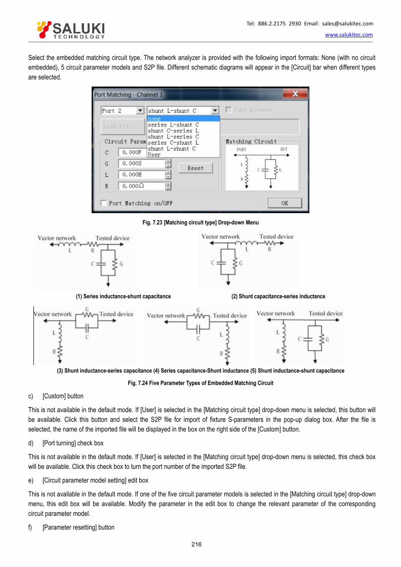
Tel: 886.2.2175 2930 Email: [email protected]
www.salukitec.com
216
Select the embedded matching circuit type. The network analyzer is provided with the following import formats: None (with no circuitembedded), 5 circuit parameter models and S2P file. Different schematic diagrams will appear in the [Circuit] bar when different typesare selected.
Fig. 7.23 [Matching circuit type] Drop-down Menu
(1) Series inductance-shunt capacitance (2) Shunt capacitance-series inductance
(3) Shunt inductance-series capacitance (4) Series capacitance-Shunt inductance (5) Shunt inductance-shunt capacitance
Fig. 7.24 Five Parameter Types of Embedded Matching Circuit
c) [Custom] button
This is not available in the default mode. If [User] is selected in the [Matching circuit type] drop-down menu is selected, this button willbe available. Click this button and select the S2P file for import of fixture S-parameters in the pop-up dialog box. After the file isselected, the name of the imported file will be displayed in the box on the right side of the [Custom] button.
d) [Port turning] check box
This is not available in the default mode. If [User] is selected in the [Matching circuit type] drop-down menu is selected, this check boxwill be available. Click this check box to turn the port number of the imported S2P file.
e) [Circuit parameter model setting] edit box
This is not available in the default mode. If one of the five circuit parameter models is selected in the [Matching circuit type] drop-downmenu, this edit box will be available. Modify the parameter in the edit box to change the relevant parameter of the correspondingcircuit parameter model.
f) [Parameter resetting] button

Tel: 886.2.2175 2930 Email: [email protected]
www.salukitec.com
217
This is not available in the default mode. If one of the five circuit parameter models is selected in the [Matching circuit type] drop-downmenu, this button will be available. Click this button to reset all the contents in the [Circuit parameter model setting] edit box.
g) [Port Matching... on/OFF] check box
Click it to enable the Port Matching... function.
h) [OK] button
Click it to make the settings in the dialog box effective for the current active channel.
2) Steps of Port Matching...
Menu path: [Calibration] > [Fixture simulator]. Click [Port Matching......] in the [Fixture simulator] sub-menu. The [Port Matching...]dialog box will appear.
Tick [Port Matching... on/OFF] in the dialog box to enable the Port Matching... function. Click the [Port selection] drop-down menu andselect the Port Matching... port.
Select the type of the embedded circuit in the drop-down menu on the right side of [Port selection]. The network analyzer is configuredwith five circuit parameter models and custom mode. The schematic diagram is shown in the [Circuit] box.
If the circuit parameter model is selected as the circuit type, edit the corresponding capacitance, inductance, resistance andconductance in the corresponding circuit parameter bar. Click [Parameter resetting] to recover the default parameter. If "User-defined"is selected as the circuit type, the [Custom] button will be available. Click the [Custom] button and select the S2P file to be used in thepop-up dialog box. The file name will be displayed in the lateral square box. Thus the [Port turning] check box will appear. Click thischeck box to customize port turning in the S2P file.
Click [OK] to complete the setting.
7.9.4. 2-port de-embedding
The network de-embedding function can be used to eliminate the characteristics of any network defined by the Touchstone data filebetween the measurement end face and DUT end face, so as to extend the corresponding calibration plane.
Fig. 7.25 Schematic Diagram of Fixture De-embedding (take the 2-port tested device as an example)
1) [2-port de-embedding] dialog box
a) [Port selection] drop-down menu
Select the vector network port number of the fixture to be de-embedded.

Tel: 886.2.2175 2930 Email: [email protected]
www.salukitec.com
218
b) [De-embedding type] drop-down menu
Select the de-embedding type in the drop-down menu on the right side of [Port selection]. The network analyzer is configured with theuser-defined de-embedding type. The contents in the schematic diagram will change if different types are selected.
c) [Import file] button
This is not available in the default mode. If [User] is selected in the [De-embedding type] drop-down menu, this button will be available.Click this button and select the S2P file for import of the fixture S-parameter in the pop-up dialog box (as shown in Fig. 7.25). After thefile is selected, the file name will be display in the box on the right side of the [Import file] button. At the same time, the relevantmaximum/minimum frequency will be updated on the frequency range display bar of the vector network port and file.
Fig. 7.26 [2-port de-embedding] Interface
d) [Port turning] check box
This is not available in the default mode. If [User] is selected in the [De-embedding type] drop-down menu, this check box will beavailable. Click this check box to turn the port number of the imported S2P file.
e) [Fixture de-embedding on/OFF] check box
Click it to enable the 2-port de-embedding function.
f) [OK] button
Click it to make the settings in the dialog box effective for the current active channel.
2) Steps of 2-port de-embedding
Menu path: [Calibration] > [Fixture simulator]. Click [2-port de-embedding...] in the [Fixture simulator] sub-menu. The [2-portde-embedding] dialog box will appear.

Tel: 886.2.2175 2930 Email: [email protected]
www.salukitec.com
219
Click the [Fixture de-embedding on/OFF] button in the dialog box to enable the 2-port fixture de- embedding function.
Click the [Port selection] drop-down menu and select the port for fixture de-embedding.
Select the de-embedding type in the drop-down menu on the right side of [Port] selection. The network analyzer is configured with theuser-defined de-embedding type.
If [User] is selected in the [De-embedding type] drop-down menu, this button will be available. Click the [Import file] button and selectthe S2P file to be used in the pop-up dialog box. The file name will be displayed in the lateral square box. The vector networkfrequency information and file frequency information will be updated.
Click the [Port turning] check box to turn the power in the custom S2P file. The corresponding schematic diagram will changeaccordingly.
Click [OK] to complete the setting.
7.9.5. Port impedance conversion...The measurement result with the port impedance as the system impedance can be transformed into the measurement result of anyimpedance.
Fig. 7.27 [Port impedance conversion...] Interface
1) [Port impedance conversion...] dialog box
a) [Port selection] drop-down menu
Select the number of the vector network port for impedance conversion....
b) [Real part of impedance] edit box
Modify the parameter in the edit box to set the impedance value to be obtained by transformation.
c) [impedance conversion... on/OFF] check box
Select it to enable the port impedance conversion... function.
d) [OK] button
Click it to make the settings in the dialog box effective for the current active channel.
2) Steps of port impedance conversion...
Menu path: [Calibration ] > [Fixture simulator]. Click [Port impedance conversion......] in the [Fixture simulator] sub-menu. The [Port

Tel: 886.2.2175 2930 Email: [email protected]
www.salukitec.com
220
impedance conversion...] dialog box will appear.
Tick the [impedance conversion... on/OFF] button in the dialog box to enable the port impedance conversion... function.
Click the [Port selection] drop-down menu and select the port for impedance conversion....
Edit the real part and imaginary part of the impedance to be transformed in the [R (real part of impedance)] an [jX (imaginary part ofimpedance)] edit box. Click [OK] to complete the setting.
7.9.6. Four-port Fixture Embedding/De-embedding
Simulate embedding/de-embedding of the four-port fixture to obtain the simulation results of the tested device afterembedding/de-embedding of part of the network.
1) [Four-port fixture embedding/de-embedding] dialog box
a) [Mode selection] drop-down menu
Select the fixture embedding/de-embedding mode. The vector network analyzer is configured with three network models (Mode A, Band C).
Fig. 7.28 Three Modes of Fixture Embedding/De-embedding
b) [Network embedding/de-embedding type] drop-down menu
The network embedding/de-embedding type is the first item of the drop-down menu of Network 1 (Network 2 is enabled in Mode C).The drop-down menu includes three options: none, de-embedding and embedding.
c) [Import file] button
Click this button and select the S4P file for import of the fixture S-parameter in the pop-up dialog box (as shown in Fig. 7.25). After thefile is selected, the file name will be display in the box on the right side of the [Import file] button.
d) [Port selection] drop-down menu
The port selection part includes the vector network port and fixture port. The [Fixture port] drop-down menu is not displayed in thedefault mode. The selected mode and network embedding/de-embedding type will be displayed in the schematic diagram. Select the
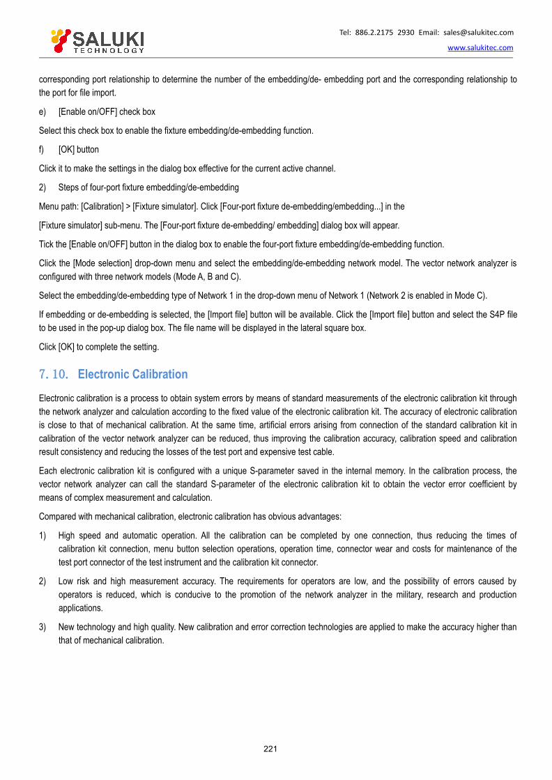
Tel: 886.2.2175 2930 Email: [email protected]
www.salukitec.com
221
corresponding port relationship to determine the number of the embedding/de- embedding port and the corresponding relationship tothe port for file import.
e) [Enable on/OFF] check box
Select this check box to enable the fixture embedding/de-embedding function.
f) [OK] button
Click it to make the settings in the dialog box effective for the current active channel.
2) Steps of four-port fixture embedding/de-embedding
Menu path: [Calibration] > [Fixture simulator]. Click [Four-port fixture de-embedding/embedding...] in the
[Fixture simulator] sub-menu. The [Four-port fixture de-embedding/ embedding] dialog box will appear.
Tick the [Enable on/OFF] button in the dialog box to enable the four-port fixture embedding/de-embedding function.
Click the [Mode selection] drop-down menu and select the embedding/de-embedding network model. The vector network analyzer isconfigured with three network models (Mode A, B and C).
Select the embedding/de-embedding type of Network 1 in the drop-down menu of Network 1 (Network 2 is enabled in Mode C).
If embedding or de-embedding is selected, the [Import file] button will be available. Click the [Import file] button and select the S4P fileto be used in the pop-up dialog box. The file name will be displayed in the lateral square box.
Click [OK] to complete the setting.
7.10. Electronic CalibrationElectronic calibration is a process to obtain system errors by means of standard measurements of the electronic calibration kit throughthe network analyzer and calculation according to the fixed value of the electronic calibration kit. The accuracy of electronic calibrationis close to that of mechanical calibration. At the same time, artificial errors arising from connection of the standard calibration kit incalibration of the vector network analyzer can be reduced, thus improving the calibration accuracy, calibration speed and calibrationresult consistency and reducing the losses of the test port and expensive test cable.
Each electronic calibration kit is configured with a unique S-parameter saved in the internal memory. In the calibration process, thevector network analyzer can call the standard S-parameter of the electronic calibration kit to obtain the vector error coefficient bymeans of complex measurement and calculation.
Compared with mechanical calibration, electronic calibration has obvious advantages:
1) High speed and automatic operation. All the calibration can be completed by one connection, thus reducing the times ofcalibration kit connection, menu button selection operations, operation time, connector wear and costs for maintenance of thetest port connector of the test instrument and the calibration kit connector.
2) Low risk and high measurement accuracy. The requirements for operators are low, and the possibility of errors caused byoperators is reduced, which is conducive to the promotion of the network analyzer in the military, research and productionapplications.
3) New technology and high quality. New calibration and error correction technologies are applied to make the accuracy higher thanthat of mechanical calibration.
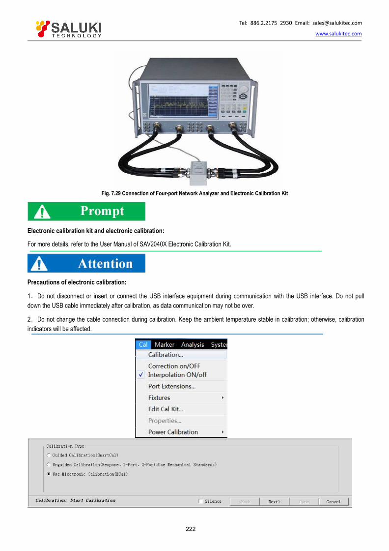
Tel: 886.2.2175 2930 Email: [email protected]
www.salukitec.com
222
Fig. 7.29 Connection of Four-port Network Analyzer and Electronic Calibration Kit
Electronic calibration kit and electronic calibration:
For more details, refer to the User Manual of SAV2040X Electronic Calibration Kit.
Precautions of electronic calibration:
1.Do not disconnect or insert or connect the USB interface equipment during communication with the USB interface. Do not pulldown the USB cable immediately after calibration, as data communication may not be over.
2.Do not change the cable connection during calibration. Keep the ambient temperature stable in calibration; otherwise, calibrationindicators will be affected.
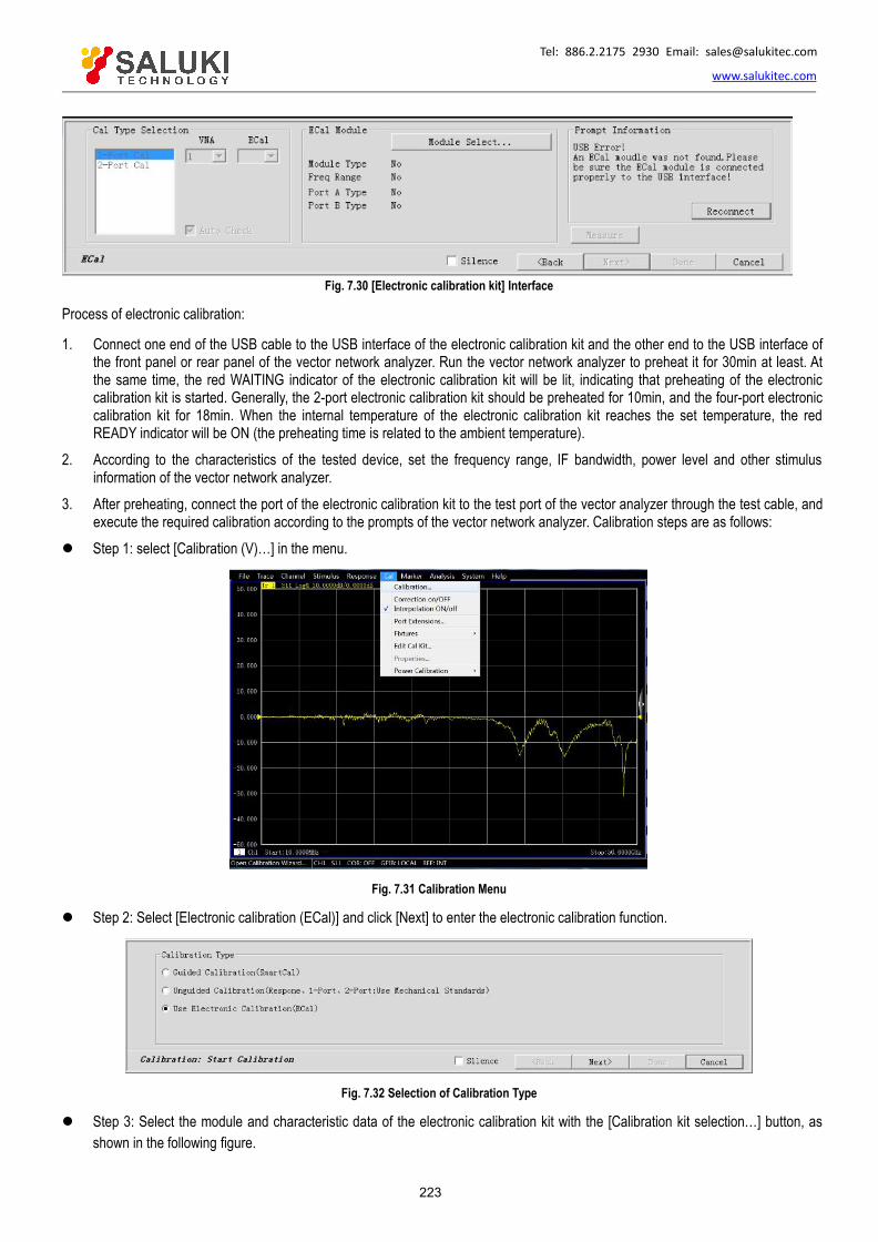
Tel: 886.2.2175 2930 Email: [email protected]
www.salukitec.com
223
Fig. 7.30 [Electronic calibration kit] Interface
Process of electronic calibration:
1. Connect one end of the USB cable to the USB interface of the electronic calibration kit and the other end to the USB interface ofthe front panel or rear panel of the vector network analyzer. Run the vector network analyzer to preheat it for 30min at least. Atthe same time, the red WAITING indicator of the electronic calibration kit will be lit, indicating that preheating of the electroniccalibration kit is started. Generally, the 2-port electronic calibration kit should be preheated for 10min, and the four-port electroniccalibration kit for 18min. When the internal temperature of the electronic calibration kit reaches the set temperature, the redREADY indicator will be ON (the preheating time is related to the ambient temperature).
2. According to the characteristics of the tested device, set the frequency range, IF bandwidth, power level and other stimulusinformation of the vector network analyzer.
3. After preheating, connect the port of the electronic calibration kit to the test port of the vector analyzer through the test cable, andexecute the required calibration according to the prompts of the vector network analyzer. Calibration steps are as follows:
Step 1: select [Calibration (V)…] in the menu.
Fig. 7.31 Calibration Menu
Step 2: Select [Electronic calibration (ECal)] and click [Next] to enter the electronic calibration function.
Fig. 7.32 Selection of Calibration Type
Step 3: Select the module and characteristic data of the electronic calibration kit with the [Calibration kit selection…] button, asshown in the following figure.

Tel: 886.2.2175 2930 Email: [email protected]
www.salukitec.com
224
Selection of electronic calibration kit and characteristic data:
If only one electronic calibration kit is connected to the vector network analyzer, the following calibration steps can be directlyperformed without calibration kit selection.
Step 4: Select the multi-port or one-port calibration in the [Selection of calibration type]
Step 5: Tick the [Automatically test port connection] function.
You can select whether to tick the [Automatically test port connection] function in the “calibration selection" combined box. If this optionis ticked (default), the vector network analyzer can test the connection of the port of the electronic calibration kit and the measurementport of the vector network analyzer, as shown in the following figure. If this option is not ticked, calibration will be done directlyaccording to the set connection mode. (If the frequency measurement range set in the vector network analyzer is beyond thefrequency range of the electronic calibration kit, the information shown in the following figure will appear. Exit the window, reset thecalibration frequency range and repeat the electronic calibration process).
Step 6: Click [Measurement] to start the measurement of electronic calibration. If necessary, click the [Interrupt sweep] tointerrupt sweep.
Step 7: Click [OK] to save calibration results after measurement.
Step 8: Connect the test cable and check the through curve (S21) after calibration. You can roughly observe whether calibrationis successful. If the vector network analyzer has good hardware performance, the amplitude of the through curve will be withinplus or minus 0.2dB. Remove the test cable from the port of the electronic calibration kit and connect the tested device to startmeasurement.

Tel: 886.2.2175 2930 Email: [email protected]
www.salukitec.com
225
8. Basic Knowledge of Network MeasurementThis chapter introduces the following contents:
Reflection measurement
Phase measurement
Amplifier parameter specifications
Complex impedance
Group delay
Absolute output power
AM-PM transformation
Linear phase offset
Reverse isolation
Small signal gain and flatness
8.1.Reflection MeasurementReflection measurement is an important part of network measurement. At first, the reflection measurement will be introduced. In orderto better understand reflection measurement, the optical wave is applied to simulate the traveling wave transmission along thetransmission line.
If any optical element such as the lens is set, part of light will be reflected by the lens, but the majority of light will be transmittedcontinuously through the lens. If the surface of the optical element is a mirror, the majority of light will be reflect, and only a little lightwill be transmitted or no light will be transmitted.
1 . Incident light 2. Reflected light 3. Transmitted light
Fig. 8.1 Light Reflection and Transmission
The RF signal will be reflected if the impedance of two connectors is different from each other. Reflection measurement is a process tomeasure the ratio of the reflected signal and incident signal. The incident signal is measured by Receiver R, and the reflected signal ismeasured by Receiver A. Therefore, the result of reflection measurement is a ratio of A and R (i.e. A/R). The reflection characteristic ofthe tested device can be fully quantified with the signal amplitude and phase information of Receiver A and R. Among the S-parameterterms, S11 represents the reflection of Port 1 (input port) of the tested device and S22 represents the reflection of Port 2 (input port) ofthe tested device. Reflection measurement aims to ensure the efficient transmission of RF energy. If energy is reflected, only a littleenergy will be transmitted to the expected place. In addition, if too much energy is reflected, the device may be burnt, such as theoutput power amplifier.
Reflection measurement expression
Summary of reflection measurement expression
8.1.1. Reflection Measurement Expression
The data of reflection measurement can be expressed in various methods according to the requirements. Various expressions are
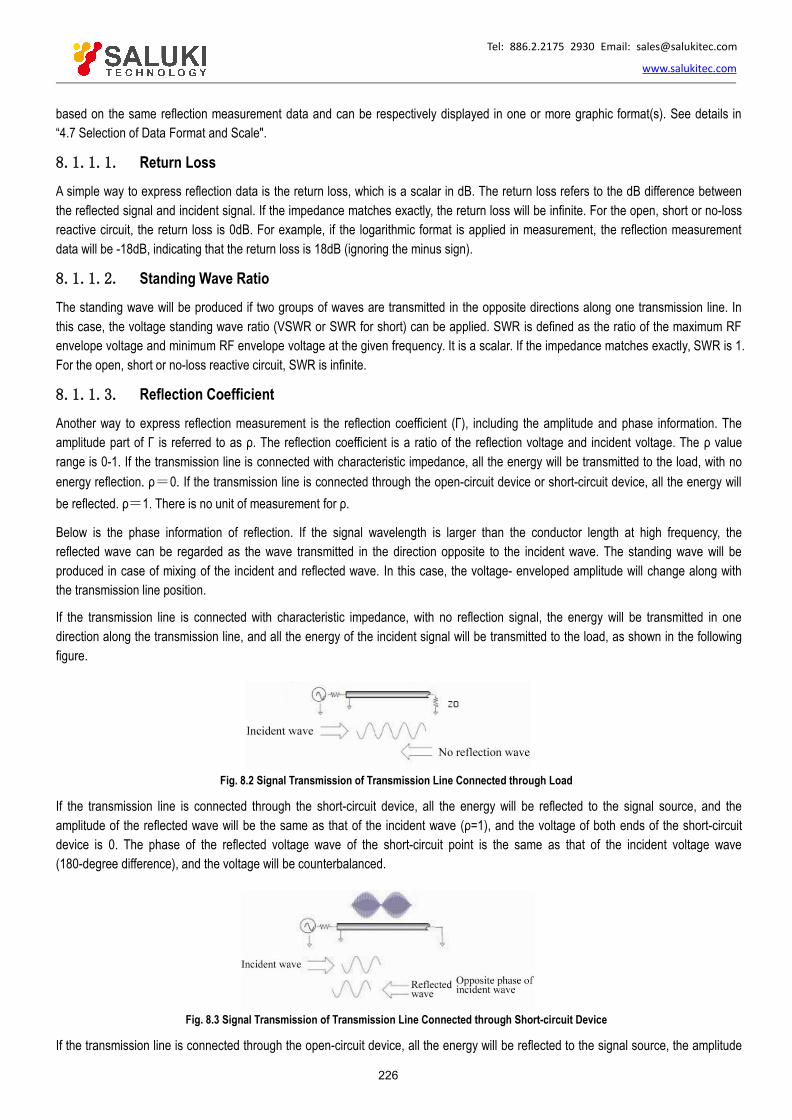
Tel: 886.2.2175 2930 Email: [email protected]
www.salukitec.com
226
based on the same reflection measurement data and can be respectively displayed in one or more graphic format(s). See details in“4.7 Selection of Data Format and Scale".
8.1.1.1. Return LossA simple way to express reflection data is the return loss, which is a scalar in dB. The return loss refers to the dB difference betweenthe reflected signal and incident signal. If the impedance matches exactly, the return loss will be infinite. For the open, short or no-lossreactive circuit, the return loss is 0dB. For example, if the logarithmic format is applied in measurement, the reflection measurementdata will be -18dB, indicating that the return loss is 18dB (ignoring the minus sign).
8.1.1.2. Standing Wave RatioThe standing wave will be produced if two groups of waves are transmitted in the opposite directions along one transmission line. Inthis case, the voltage standing wave ratio (VSWR or SWR for short) can be applied. SWR is defined as the ratio of the maximum RFenvelope voltage and minimum RF envelope voltage at the given frequency. It is a scalar. If the impedance matches exactly, SWR is 1.For the open, short or no-loss reactive circuit, SWR is infinite.
8.1.1.3. Reflection Coefficient
Another way to express reflection measurement is the reflection coefficient (Γ), including the amplitude and phase information. Theamplitude part of Γ is referred to as ρ. The reflection coefficient is a ratio of the reflection voltage and incident voltage. The ρ valuerange is 0-1. If the transmission line is connected with characteristic impedance, all the energy will be transmitted to the load, with noenergy reflection. ρ=0. If the transmission line is connected through the open-circuit device or short-circuit device, all the energy willbe reflected. ρ=1. There is no unit of measurement for ρ.
Below is the phase information of reflection. If the signal wavelength is larger than the conductor length at high frequency, thereflected wave can be regarded as the wave transmitted in the direction opposite to the incident wave. The standing wave will beproduced in case of mixing of the incident and reflected wave. In this case, the voltage- enveloped amplitude will change along withthe transmission line position.
If the transmission line is connected with characteristic impedance, with no reflection signal, the energy will be transmitted in onedirection along the transmission line, and all the energy of the incident signal will be transmitted to the load, as shown in the followingfigure.
Fig. 8.2 Signal Transmission of Transmission Line Connected through Load
If the transmission line is connected through the short-circuit device, all the energy will be reflected to the signal source, and theamplitude of the reflected wave will be the same as that of the incident wave (ρ=1), and the voltage of both ends of the short-circuitdevice is 0. The phase of the reflected voltage wave of the short-circuit point is the same as that of the incident voltage wave(180-degree difference), and the voltage will be counterbalanced.
Fig. 8.3 Signal Transmission of Transmission Line Connected through Short-circuit Device
If the transmission line is connected through the open-circuit device, all the energy will be reflected to the signal source, the amplitude
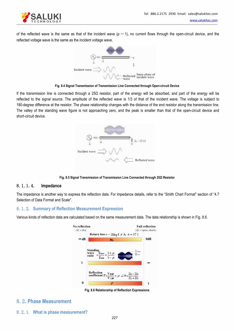
Tel: 886.2.2175 2930 Email: [email protected]
www.salukitec.com
227
of the reflected wave is the same as that of the incident wave (ρ= 1), no current flows through the open-circuit device, and thereflected voltage wave is the same as the incident voltage wave.
Fig. 8.4 Signal Transmission of Transmission Line Connected through Open-circuit Device
If the transmission line is connected through a 25Ω resistor, part of the energy will be absorbed, and part of the energy will bereflected to the signal source. The amplitude of the reflected wave is 1/3 of that of the incident wave. The voltage is subject to180-degree difference at the resistor. The phase relationship changes with the distance of the end resistor along the transmission line.The valley of the standing wave figure is not approaching zero, and the peak is smaller than that of the open-circuit device andshort-circuit device.
Fig. 8.5 Signal Transmission of Transmission Line Connected through 25Ω Resistor
8.1.1.4. Impedance
The impedance is another way to express the reflection data. For impedance details, refer to the “Smith Chart Format" section of “4.7Selection of Data Format and Scale".
8.1.2. Summary of Reflection Measurement ExpressionVarious kinds of reflection data are calculated based on the same measurement data. The data relationship is shown in Fig. 8.6.
Fig. 8.6 Relationship of Reflection Expressions
8.2.Phase Measurement
8.2.1. What is phase measurement?

Tel: 886.2.2175 2930 Email: [email protected]
www.salukitec.com
228
It is important to understand the amplitude and phase information of the tested device to integrate high-level devices. Similar to theamplitude measurement, the S-parameter is also applied in phase measurement. Phase measurement is a kind of relative (ratio)measurement instead of absolute measurement. The phase of the signal into the device (incident signal) and the response signal arecompared in phase measurement. The response signal may be reflected signal or transmitted signal. Given that the analyzer isaccurately calibrated, the phase difference (i.e. phase shift) of two signals is the measurement result of phase characteristics of thetested device. The following figure shows the phase offset between the incident signal and transmitted signal observed through theoscilloscope.
Fig. 8.7 Phase Shift between Signals
8.2.2. Why to perform phase measurement?
Phase measurement is an important function of the vector network analyzer. Fig. 8.8 shows the reasons for accurate measurement ofthe amplitude and phase.
Fig. 8.8 Reasons for Accurate Amplitude and Phase Measurement
If the element and circuit are used to transmit signals in the communication system, signal distortion must be within the normal limits.The signal distortion can be divided into two types.
1) Linear distortion: refer to the failure to keep the flat amplitude and linear phase shift within the relevant frequency range as aresult of frequency changes.
2) Nonlinear distortion: refer to the new spectrum component of the circuit, such as AM-PM transformation.
It is important to accurately measure the amplitude and phase characteristics of the element or circuit, so as to ensure the efficienttransmission or adsorption of energy in the circuit and prevent the distortion in signal transmission. A good example to preventdistortion is to measure the complex impedance of the antenna.
8.2.3. Use of Phase Format of Analyzer
The phase format of the analyzer is used to display the phase changes over the frequency or power. The phase difference beyond±180° between the reference signal and response signal cannot be measured by the analyzer. If the phase value varies from +180° to-180°, the sawtooth type phase measurement track will be displayed on the analyzer. The sawtooth waveform may not reach +180° or-180° sometimes in measurement at the discrete frequency points. The data points of +180° and -180° may not be the points ofsweep measurement.
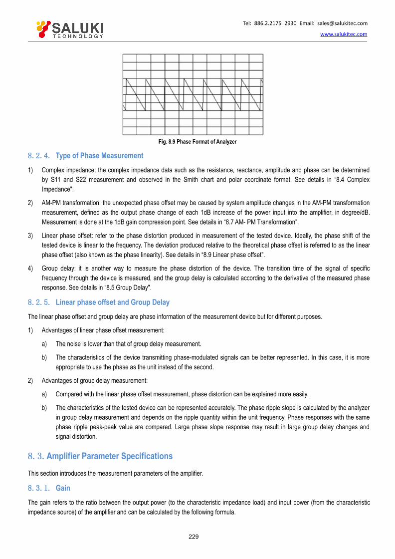
Tel: 886.2.2175 2930 Email: [email protected]
www.salukitec.com
229
Fig. 8.9 Phase Format of Analyzer
8.2.4. Type of Phase Measurement
1) Complex impedance: the complex impedance data such as the resistance, reactance, amplitude and phase can be determinedby S11 and S22 measurement and observed in the Smith chart and polar coordinate format. See details in “8.4 ComplexImpedance".
2) AM-PM transformation: the unexpected phase offset may be caused by system amplitude changes in the AM-PM transformationmeasurement, defined as the output phase change of each 1dB increase of the power input into the amplifier, in degree/dB.Measurement is done at the 1dB gain compression point. See details in “8.7 AM- PM Transformation".
3) Linear phase offset: refer to the phase distortion produced in measurement of the tested device. Ideally, the phase shift of thetested device is linear to the frequency. The deviation produced relative to the theoretical phase offset is referred to as the linearphase offset (also known as the phase linearity). See details in “8.9 Linear phase offset".
4) Group delay: it is another way to measure the phase distortion of the device. The transition time of the signal of specificfrequency through the device is measured, and the group delay is calculated according to the derivative of the measured phaseresponse. See details in “8.5 Group Delay".
8.2.5. Linear phase offset and Group DelayThe linear phase offset and group delay are phase information of the measurement device but for different purposes.
1) Advantages of linear phase offset measurement:
a) The noise is lower than that of group delay measurement.
b) The characteristics of the device transmitting phase-modulated signals can be better represented. In this case, it is moreappropriate to use the phase as the unit instead of the second.
2) Advantages of group delay measurement:
a) Compared with the linear phase offset measurement, phase distortion can be explained more easily.
b) The characteristics of the tested device can be represented accurately. The phase ripple slope is calculated by the analyzerin group delay measurement and depends on the ripple quantity within the unit frequency. Phase responses with the samephase ripple peak-peak value are compared. Large phase slope response may result in large group delay changes andsignal distortion.
8.3.Amplifier Parameter Specifications
This section introduces the measurement parameters of the amplifier.
8.3.1. GainThe gain refers to the ratio between the output power (to the characteristic impedance load) and input power (from the characteristicimpedance source) of the amplifier and can be calculated by the following formula.

Tel: 886.2.2175 2930 Email: [email protected]
www.salukitec.com
230
The output power of the amplifier is proportional to the input power in the case of small signal. The small-signal gain is within the linearzone. With the power level of the input signal increasing, the amplifier will be saturated, and the output power will reach the limit,leading to gain decline. The large signal gain is within the nonlinear zone.
8.3.2. Gain FlatnessThe gain flatness refers to the gain change of the amplifier within the working frequency range. See details in“8.10 Small Signal Gainand Flatness".
8.3.3. Reverse Isolation
Reverse isolation is applied to measure the transmission between the output end and input end. Similar to gain measurement, onlythe stimulus signal is applied to the output end of the amplifier. See details in “8.9 Reverse Isolation".
8.3.4. Gain Drift Changes over Time (temperature and bias)
The gain drift refers to the maximum gain change over time, with the other parameters unchanged. It is a function of the time. Thegain drift related to other parameters can be measured, such as the gain deviation over the temperature, humidity and bias voltage.
8.3.5. Linear phase offsetRefer to the deviation of linear shifts. Ideally, the phase shift of the amplifier is a linear function of the frequency. See details in “8.8Linear phase offset".
8.3.6. Group DelayThe group delay refers to the transition time of the signal through the amplifier. It is a function of the frequency. The ideal linear phaseshift has a constant change rate over the frequency. In this case, the group delay is a constant. In the actual measurement, the groupdelay is calculated by the following formula:
See details in “8.5 Group Delay".
8.3.7. Return Loss (standing wave ratio, ρ)
The return loss refers to the reflection matching of the amplifier relative to the system impedance Z0 in measurement of the input oroutput port. It can be calculated by the following formula:
8.3.8. Complex Impedance
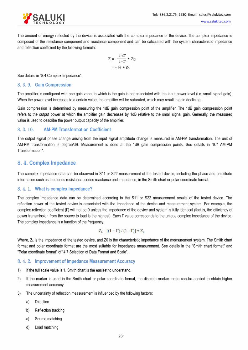
Tel: 886.2.2175 2930 Email: [email protected]
www.salukitec.com
231
The amount of energy reflected by the device is associated with the complex impedance of the device. The complex impedance iscomposed of the resistance component and reactance component and can be calculated with the system characteristic impedanceand reflection coefficient by the following formula:
See details in “8.4 Complex Impedance".
8.3.9. Gain CompressionThe amplifier is configured with one gain zone, in which is the gain is not associated with the input power level (i.e. small signal gain).When the power level increases to a certain value, the amplifier will be saturated, which may result in gain declining.
Gain compression is determined by measuring the 1dB gain compression point of the amplifier. The 1dB gain compression pointrefers to the output power at which the amplifier gain decreases by 1dB relative to the small signal gain. Generally, the measuredvalue is used to describe the power output capacity of the amplifier.
8.3.10. AM-PM Transformation CoefficientThe output signal phase change arising from the input signal amplitude change is measured in AM-PM transformation. The unit ofAM-PM transformation is degree/dB. Measurement is done at the 1dB gain compression points. See details in “8.7 AM-PMTransformation".
8.4.Complex Impedance
The complex impedance data can be observed in S11 or S22 measurement of the tested device, including the phase and amplitudeinformation such as the series resistance, series reactance and impedance, in the Smith chart or polar coordinate format.
8.4.1. What is complex impedance?
The complex impedance data can be determined according to the S11 or S22 measurement results of the tested device. Thereflection power of the tested device is associated with the impedance of the device and measurement system. For example, thecomplex reflection coefficient (Γ) will not be 0 unless the impedance of the device and system is fully identical (that is, the efficiency ofpower transmission from the source to load is the highest). Each Γ value corresponds to the unique complex impedance of the device.The complex impedance is a function of the frequency.
Where, ZL is the impedance of the tested device, and Z0 is the characteristic impedance of the measurement system. The Smith chartformat and polar coordinate format are the most suitable for impedance measurement. See details in the “Smith chart format" and"Polar coordinate format" of “4.7 Selection of Data Format and Scale".
8.4.2. Improvement of Impedance Measurement Accuracy1) If the full scale value is 1, Smith chart is the easiest to understand.
2) If the marker is used in the Smith chart or polar coordinate format, the discrete marker mode can be applied to obtain highermeasurement accuracy.
3) The uncertainty of reflection measurement is influenced by the following factors:
a) Direction
b) Reflection tracking
c) Source matching
d) Load matching

Tel: 886.2.2175 2930 Email: [email protected]
www.salukitec.com
232
The influence of these factors can be reduced in the full 2-port calibration. If the output end of the tested device is connected with ahigh-quality load, the same measurement accuracy can be achieved by means of one-port calibration.
Fig. 8.10 Connection in Impedance Measurement
4) If the tested device is connected between two ports of the analyzer after one-port calibration, it is recommended to connect a10dB attenuator to the output end of the tested device to improve the measurement accuracy. If the full 2-port calibration hasbeen done, the attenuator is not required as the load matching error is modified in the full-port calibration.
5) If the 2-port device is connected to one port of the analyzer after one-port calibration, a high-quality load (such as the standardload of the calibration kit) must be connected to the output port of the device.
8.4.3. Steps of Complex Impedance Measurement1) Reset the analyzer.
2) Set and calibrate the analyzer.
3) Connector shown in Fig. 8.10 for S11 or S22 measurement.
4) Observe the impedance data:
a) Select the Smith chart format.
b) Set the scale of the displayed measurement results to facilitate observation.
c) Open the marker, and move the marker along the trace to read the resistance and reactance component of the compleximpedance of the data point.
d) Print or save the data.
5) Observe the admittance data (if necessary):
a) Open the marker and select the G+jB marker format to read the admittance data.
b) Set the scale of the displayed measurement results to facilitate observation.
c) Move the marker along the trace to read the conductance and susceptance component of the complex admittance of thedata point, in siemens (S).
d) Print or save the data.
6) Observe the amplitude and phase of the reflection coefficient:
a) Select the Smith chart or polar coordinate format.
b) Open the marker and select the logarithmic/phase or linear/phase format.
c) Set the scale of the displayed measurement results to facilitate observation.
d) Move the marker along the trace to read the amplitude and phase information of the data point.
e) Print or save the data.

Tel: 886.2.2175 2930 Email: [email protected]
www.salukitec.com
233
8.5.Group Delay
The phase distortion of the tested device is measured in group delay measurement. The group delay refers to the actual transitiontime of the signal through the tested device and changes over the frequency. The aperture of group delay measurement must bespecified to describe the group delay indicator.
8.5.1. What is group delay?
The group delay refers to:
1) Measure of phase distortion of the device.
2) Relationship between the signal transition time through the device and the frequency.
3) Derivative of the phase characteristic of the device relative to the frequency.
Fig. 8.11 Phase Shift and Group Delay
Group delay
Φ is in radian, ω in radian/second, θ in degree and f in Hz.
The phase characteristic of the device includes the linear phase shift component and high-order phase shift component.
1) Linear phase shift component: refer to the average transition time of the signal, indicating the electrical length of the device.
2) High-order phase shift component: refer to the transition time change over the frequency, a cause of signal distortion.
Fig. 8.12 Group Delay
In the group delay measurement:
1) The linear phase shift component represents the average group delay.
2) The high-order phase shift component represents the average group delay deviation (group delay ripple).
3) Similar to the linear phase offset resulting in distortion, the group delay deviation will also result in signal distortion.
4) The trace of group delay measurement indicates the passing time of each frequency signal through the tested device.
The group delay of the analyzer is calculated in the following methods:
Group delay
Φ is in radian, ω in radian/second, θ in degree and f in Hz.
1) Calculate the phase change (-dΦ) according to the phase data.
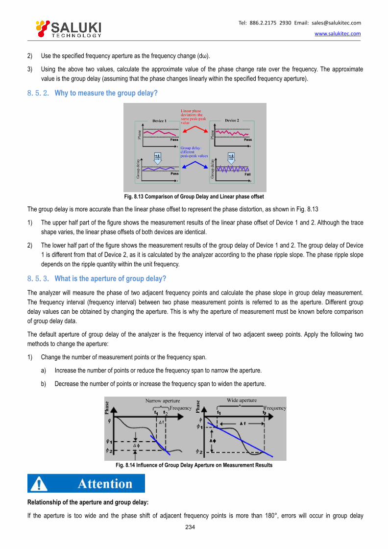
Tel: 886.2.2175 2930 Email: [email protected]
www.salukitec.com
234
2) Use the specified frequency aperture as the frequency change (dω).
3) Using the above two values, calculate the approximate value of the phase change rate over the frequency. The approximatevalue is the group delay (assuming that the phase changes linearly within the specified frequency aperture).
8.5.2. Why to measure the group delay?
Fig. 8.13 Comparison of Group Delay and Linear phase offset
The group delay is more accurate than the linear phase offset to represent the phase distortion, as shown in Fig. 8.13
1) The upper half part of the figure shows the measurement results of the linear phase offset of Device 1 and 2. Although the traceshape varies, the linear phase offsets of both devices are identical.
2) The lower half part of the figure shows the measurement results of the group delay of Device 1 and 2. The group delay of Device1 is different from that of Device 2, as it is calculated by the analyzer according to the phase ripple slope. The phase ripple slopedepends on the ripple quantity within the unit frequency.
8.5.3. What is the aperture of group delay?
The analyzer will measure the phase of two adjacent frequency points and calculate the phase slope in group delay measurement.The frequency interval (frequency interval) between two phase measurement points is referred to as the aperture. Different groupdelay values can be obtained by changing the aperture. This is why the aperture of measurement must be known before comparisonof group delay data.
The default aperture of group delay of the analyzer is the frequency interval of two adjacent sweep points. Apply the following twomethods to change the aperture:
1) Change the number of measurement points or the frequency span.
a) Increase the number of points or reduce the frequency span to narrow the aperture.
b) Decrease the number of points or increase the frequency span to widen the aperture.
Fig. 8.14 Influence of Group Delay Aperture on Measurement Results
Relationship of the aperture and group delay:
If the aperture is too wide and the phase shift of adjacent frequency points is more than 180°, errors will occur in group delay
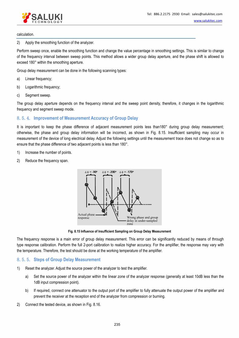
Tel: 886.2.2175 2930 Email: [email protected]
www.salukitec.com
235
calculation.
2) Apply the smoothing function of the analyzer.
Perform sweep once, enable the smoothing function and change the value percentage in smoothing settings. This is similar to changeof the frequency interval between sweep points. This method allows a wider group delay aperture, and the phase shift is allowed toexceed 180° within the smoothing aperture.
Group delay measurement can be done in the following scanning types:
a) Linear frequency;
b) Logarithmic frequency;
c) Segment sweep.
The group delay aperture depends on the frequency interval and the sweep point density, therefore, it changes in the logarithmicfrequency and segment sweep mode.
8.5.4. Improvement of Measurement Accuracy of Group Delay
It is important to keep the phase difference of adjacent measurement points less than180° during group delay measurement;otherwise, the phase and group delay information will be incorrect, as shown in Fig. 8.15. Insufficient sampling may occur inmeasurement of the device of long electrical delay. Adjust the following settings until the measurement trace does not change so as toensure that the phase difference of two adjacent points is less than 180°.
1) Increase the number of points.
2) Reduce the frequency span.
Fig. 8.15 Influence of Insufficient Sampling on Group Delay Measurement
The frequency response is a main error of group delay measurement. This error can be significantly reduced by means of throughtype response calibration. Perform the full 2-port calibration to realize higher accuracy. For the amplifier, the response may vary withthe temperature. Therefore, the test should be done at the working temperature of the amplifier.
8.5.5. Steps of Group Delay Measurement
1) Reset the analyzer. Adjust the source power of the analyzer to test the amplifier.
a) Set the source power of the analyzer within the linear zone of the analyzer response (generally at least 10dB less than the1dB input compression point).
b) If required, connect one attenuator to the output port of the amplifier to fully attenuate the output power of the amplifier andprevent the receiver at the reception end of the analyzer from compression or burning.
2) Connect the tested device, as shown in Fig. 8.16.
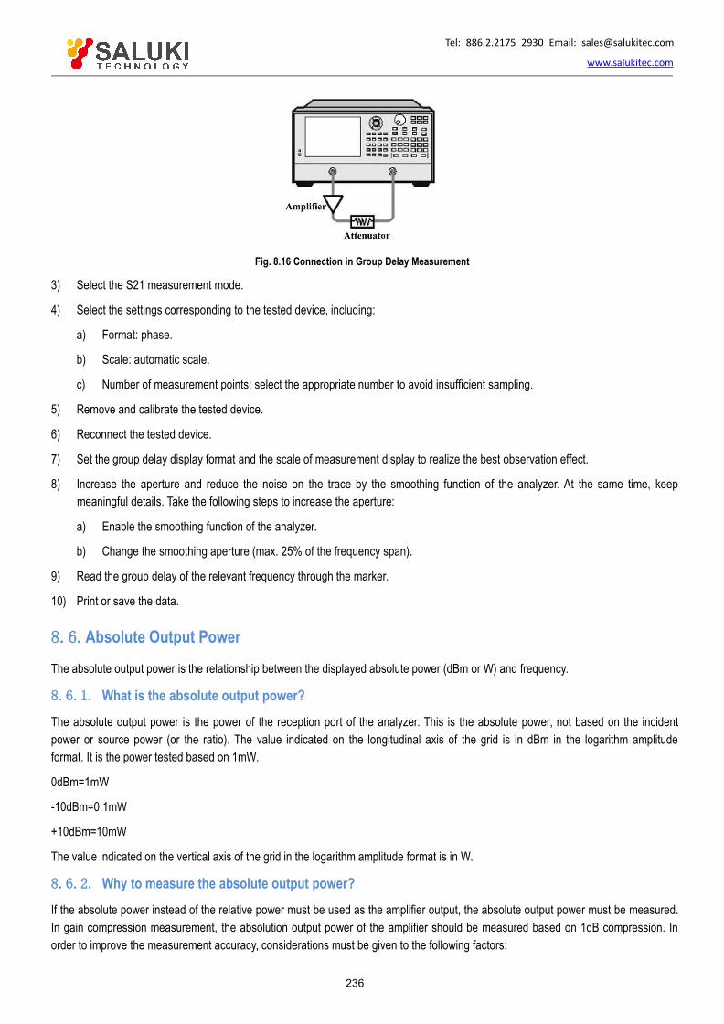
Tel: 886.2.2175 2930 Email: [email protected]
www.salukitec.com
236
Fig. 8.16 Connection in Group Delay Measurement
3) Select the S21 measurement mode.
4) Select the settings corresponding to the tested device, including:
a) Format: phase.
b) Scale: automatic scale.
c) Number of measurement points: select the appropriate number to avoid insufficient sampling.
5) Remove and calibrate the tested device.
6) Reconnect the tested device.
7) Set the group delay display format and the scale of measurement display to realize the best observation effect.
8) Increase the aperture and reduce the noise on the trace by the smoothing function of the analyzer. At the same time, keepmeaningful details. Take the following steps to increase the aperture:
a) Enable the smoothing function of the analyzer.
b) Change the smoothing aperture (max. 25% of the frequency span).
9) Read the group delay of the relevant frequency through the marker.
10) Print or save the data.
8.6.Absolute Output Power
The absolute output power is the relationship between the displayed absolute power (dBm or W) and frequency.
8.6.1. What is the absolute output power?The absolute output power is the power of the reception port of the analyzer. This is the absolute power, not based on the incidentpower or source power (or the ratio). The value indicated on the longitudinal axis of the grid is in dBm in the logarithm amplitudeformat. It is the power tested based on 1mW.
0dBm=1mW
-10dBm=0.1mW
+10dBm=10mW
The value indicated on the vertical axis of the grid in the logarithm amplitude format is in W.
8.6.2. Why to measure the absolute output power?If the absolute power instead of the relative power must be used as the amplifier output, the absolute output power must be measured.In gain compression measurement, the absolution output power of the amplifier should be measured based on 1dB compression. Inorder to improve the measurement accuracy, considerations must be given to the following factors:

Tel: 886.2.2175 2930 Email: [email protected]
www.salukitec.com
237
1) If necessary, fully attenuate the output power of the amplifier. Too high power may lead to the following results:
a) The output power is higher than the input compression level of the receiver of the analyzer, which may lead to inaccuratemeasurement results.
b) The receiver of the analyzer may be burnt.
2) Attenuate the output power of the amplifier with the attenuator or coupler.
3) The amplifier has different response values corresponding to temperature differences. The test must be done at the workingtemperature of the amplifier.
8.6.3. Steps of Measurement of Absolute Output Power
1) Reset the analyzer.
2) Select the non-ratio power measurement (the source is set on Port 1 and Receiver B is used for input).
3) Set the source power of the analyzer as 0dBm.
4) As shown in Fig. 8.17, connect the amplifier and provide the DC bias. If necessary, use an external attenuator to fully attenuatethe output power of the amplifier so as to prevent the receiver on Port 2 of the analyzer from compression or burning.
Fig. 8.17 Connection in Absolute Output Power Measurement
1) Select the analyzer settings corresponding to the amplifier to be tested.
2) Remove the amplifier, and connect the attenuator and cable between two ports. Apply the trace operation function and save thedata trace into the memory. Apply the data/saving function for normalization. If the attenuator and cable are used in amplifiermeasurement, they must be included in normalization measurement.
3) Reconnect the amplifier.
4) Set the scale of measurement display to realize the best observation effect. Read the absolute output power corresponding tothe frequency through the marker.
5) Print or save the data.
8.7.AM-PM Transformation
AM-PM transformation of the amplifier represents the phase offset caused by system amplitude changes.
8.7.1. What is AM-PM transformation?AM-PM transformation represents the unexpected phase offset (PM) caused by system amplitude changes (AM). The unexpectedphase offset (PM) in the communication system may be caused for the following reasons:
1) Accidental amplitude change (AM):
a) Power fluctuation;

Tel: 886.2.2175 2930 Email: [email protected]
www.salukitec.com
238
b) Thermal drift;
c) Multipath attenuation.
2) Deliberate signal amplitude modulation:
a) QAM (quadrature amplitude modulation);
b) Sudden pulse modulation.
AM-PM transformation is generally defined as the output phase change in radian/dB, corresponding to 1dB increase of the sweeppower applied on the input end of the amplifier (at the 1dB gain compression point). The phase response of the ideal amplifier is notassociated with the power level of the input signal.
8.7.2. Why to measure AM-PM transformation?AM-PM transformation is a key parameter in the following phase (angle) modulation system.
1) FM
2) QPSK
3) 16QAM
The unexpected phase offset (PM) will result in deterioration of the analog signal performance or increase of the bit error rate (BER) ofthe digital communication system. It is easy to measure the bit error rate (BER) of the digital system, but this is not helpful tounderstand the root causes of bit errors. AM-PM transformation is one of the main factors resulting in bit errors. Therefore, it is criticalto quantify this parameter in the communication system. The following I/O figure shows why bit errors are produced in AM-PMtransformation.
Fig. 8.18 Bit Errors in AM-PM Transformation
1) The expected state change is from the small solid-line vector into large solid-line vector.
2) As a result of AM-PM transformation, the large solid-line vector may end like that shown by the dotted line in the actual situation.This is caused by the phase shift arising from changes of the input power level.
3) For the 64QAM signal (only the quadrant is drawn) shown in Fig. 8.18, bit errors occur in the statistics if the noise circles of eachstate are overlapped.
8.7.3. Factors Related to Measurement AccuracyWhen the network analyzer is used to measure AM-PM transformation, the frequency of the amplitude modulation signal isapproximate to the reciprocal of the sweep time. Even if the highest scanning power is set, the modulation frequency is low (generallyless than 10Hz). This may result in slight temperature changes of the tested device in the sweep process, especially the thermal massof the amplifier is small (typically for the unsealed device). If the nonlinear characteristic of the amplifier is sensitive to thermalchanges, the measurement result obtained in this method may have errors. In order to improve the measurement accuracy,considerations should be given to the following factors.
1) The amplifier response may be vary with the temperature. The test must be done at the working temperature of the amplifier.

Tel: 886.2.2175 2930 Email: [email protected]
www.salukitec.com
239
2) If necessary, fully attenuate the output power of the amplifier. Too high power may lead to the following results:
a) The output power is higher than the input compression level of the receiver of the analyzer, which may lead to inaccuratemeasurement results.
b) The receiver of the analyzer may be burnt.
3) Attenuate the output power of the amplifier with the attenuator or coupler.
4) The influence of the frequency response of the attenuator or coupler must be taken into consideration during calibration. Theyare part of the test system and must be included in the calibration process. The influence of such accessories can be reduced oreliminated by the perfect technology of error correction.
5) The frequency response is an error which plays a dominant role in AM-PM transformation measurement. The through typeresponse calibration can be applied to significantly reduce the error.
8.7.4. Step of AM-PM Transformation Measurement1) Reset the analyzer.
2) Select S21 measurement in the power sweep mode.
3) Set the starting and ending power level of power sweep of the analyzer. The starting power level should be within the linear zone(generally at least 10dB less than the 1dB compression point) of the amplifier response, and the ending power level should bewithin the compression zone of the amplifier response.
4) If necessary, use the external attenuator or coupler to fully attenuate the output power of the amplifier and prevent the receiveron Port 2 of the analyzer from compression or burning.
5) As shown in Fig. 8.19, connect the amplifier and provide the DC bias.
Fig. 8.19 Connection in AM-PM Transformation Measurement
6) Select the analyzer settings corresponding to the tested amplifier so as to perform gain compression measurement in the powersweep mode at the selected frequency. See details in "Appendix 5 Gain Compression Measurement of Amplifier".
7) Remove and calibrate the amplifier. The attenuator, coupler and cable used in amplifier measurement must be included incalibration.
8) Reconnect the amplifier, open the marker R and set the marker at the 1dB gain compression point of the amplifier. Open thesecond marker, activate the Δmarker mode, and set the stimulus value of the second marker as -1dBm.
9) Change S21 measurement from the logarithmic amplitude format into the phase format (requiring no re- calibration).
10) Read the phase difference between the marker. This value is the AM-PM transformation coefficient at the 1dB gain compressionpoint.
11) Print or save the data.

Tel: 886.2.2175 2930 Email: [email protected]
www.salukitec.com
240
8.8.Linear phase offset
The linear phase offset refers to the phase distortion of the device. The electrical delay function of the analyzer is applied inmeasurement to eliminate the linear part of the phase shift and realize high-resolution nonlinear part, i.e. linear phase offset.
8.8.1. What is linear phase shift?The signal wavelength will decrease with the incident signal frequency increasing during signal transmission. In this case, the obviousphase shift will be produced. The phase shift is linear when the phase response of the device is proportional to the frequency. Thetrace indicating the relationship between the phase and frequency on the analyzer is an oblique line. The slope is proportional to theelectrical length of the device. The phase shift must be linear for signal transmission without distortion.
8.8.2. What is linear phase offset?In the actual cases, the delay time of many devices corresponding to some frequencies is longer than that corresponding to the otherfrequencies so as to form the nonlinear phase shift, including distortion of many frequency component signals. One method todetermine the nonlinear phase shift is to measure the linear phase offset.
As phase distortion is caused by linear phase offset, the linear part of the phase response should be removed in measurement. Thiscan be realized by the electrical delay function of the analyzer. If the electrical length of the tested device is removed mathematically,the linear phase offset or phase distortion will be left.
8.8.3. Why to measure the linear phase offset?
Linear phase offset measurement has the following advantages:
a) The measurement result is the phase data, instead of the group delay data in second. The phase data may be more usable forthe device transmitting modulation signals.
b) Provide a measurement method with noise lower than that of group delay measurement.
8.8.4. Use of Electrical Delay Function
The electrical delay characteristic of the analyzer has the following functions:
1) Simulate the transmission line of adjustable length and no loss to facilitate the installation in or removal from the signal path.
2) Compensate changes of the electrical length of the tested device.
3) Make the phase measurement trace on the analyzer flat, to realize the high-resolution observation of the track and find nonlineardetails of the phase.
4) Provide a method to easily observe the linear phase offset of the tested device.
Fig. 8.20 Observation of Linear phase offset by Electrical Delay Function
See electrical delay details in “6.5.1 Electrical Delay".
8.8.5. Factors Related to Measurement AccuracyThe frequency response is an error which plays a dominant role in linear phase offset measurement. The through type responsecalibration can be applied to significantly reduce the error. In order to achieve higher accuracy, the full 2-port calibration should be
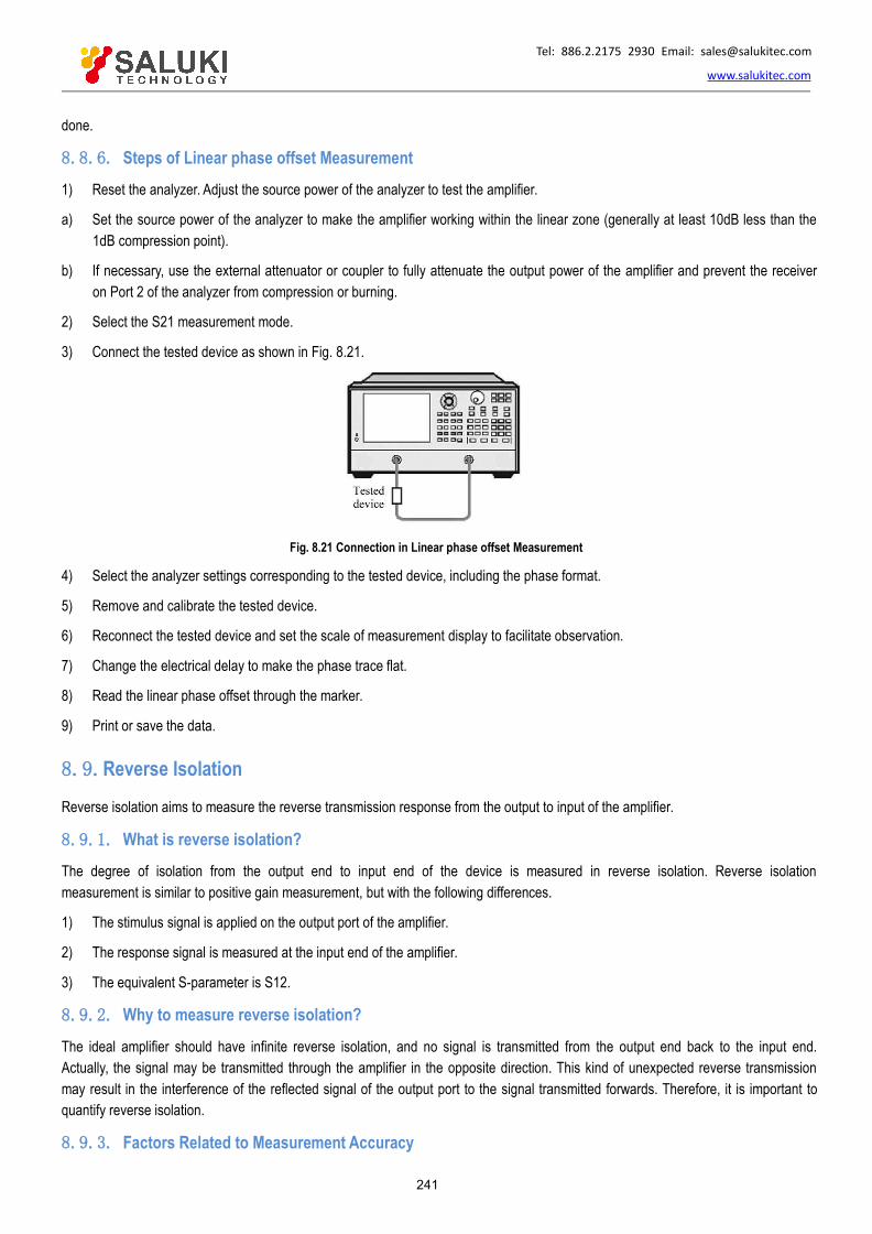
Tel: 886.2.2175 2930 Email: [email protected]
www.salukitec.com
241
done.
8.8.6. Steps of Linear phase offset Measurement1) Reset the analyzer. Adjust the source power of the analyzer to test the amplifier.
a) Set the source power of the analyzer to make the amplifier working within the linear zone (generally at least 10dB less than the1dB compression point).
b) If necessary, use the external attenuator or coupler to fully attenuate the output power of the amplifier and prevent the receiveron Port 2 of the analyzer from compression or burning.
2) Select the S21 measurement mode.
3) Connect the tested device as shown in Fig. 8.21.
Fig. 8.21 Connection in Linear phase offset Measurement
4) Select the analyzer settings corresponding to the tested device, including the phase format.
5) Remove and calibrate the tested device.
6) Reconnect the tested device and set the scale of measurement display to facilitate observation.
7) Change the electrical delay to make the phase trace flat.
8) Read the linear phase offset through the marker.
9) Print or save the data.
8.9.Reverse Isolation
Reverse isolation aims to measure the reverse transmission response from the output to input of the amplifier.
8.9.1. What is reverse isolation?The degree of isolation from the output end to input end of the device is measured in reverse isolation. Reverse isolationmeasurement is similar to positive gain measurement, but with the following differences.
1) The stimulus signal is applied on the output port of the amplifier.
2) The response signal is measured at the input end of the amplifier.
3) The equivalent S-parameter is S12.
8.9.2. Why to measure reverse isolation?
The ideal amplifier should have infinite reverse isolation, and no signal is transmitted from the output end back to the input end.Actually, the signal may be transmitted through the amplifier in the opposite direction. This kind of unexpected reverse transmissionmay result in the interference of the reflected signal of the output port to the signal transmitted forwards. Therefore, it is important toquantify reverse isolation.
8.9.3. Factors Related to Measurement Accuracy

Tel: 886.2.2175 2930 Email: [email protected]
www.salukitec.com
242
As the amplifier generally has high loss in the reverse direction, the attenuator or coupler is not required to protect the receiver of Port1 in reverse transmission measurement. In case of no attenuator, the dynamic range and measurement accuracy will be improved.The source power can be increased to improve the dynamic range and accuracy.
The power must not be overloaded forward sweep or full 2-port calibration.
With the attenuator eliminated and RF power increased, the receiver of Port 2 of the analyzer may be burnt in forward sweep. Thus,forward sweep or full 2-port calibration must not be done until the forward power is low enough, which cannot result in burning of thereceiver of Port 2 of the analyzer.
If the tested amplifier is highly isolated, the level of the reverse signal may be close to the base noise or crosstalk level of the receiver.In order to reduce the base noise, the averaging function can be applied. The dynamic range and accuracy of measurement can beimproved by increasing the averaging times or reducing the IF bandwidth, at the sacrifice of measurement speed.
1) If the measurement accuracy is affected by the crosstalk, the through type response and isolation calibration can beimplemented to reduce crosstalk errors. Use the same averaging factor and IF bandwidth during calibration and measurement.
2) The frequency response of the test is a main error source in reverse isolation measurement. It can be eliminated by through typeresponse or through type response/isolation calibration.
3) If the temperature varies, the amplifier response may be thoroughly difference. The test should be done at the workingtemperature of the amplifier.
8.9.4. Steps of Reverse Isolation Measurement
1) Reset the analyzer.
2) Select the S12 measurement type.
3) Connect the amplifier as shown in Fig. 8.22 and provide the DC bias.
Fig. 8.22 Connection in Reverse Isolation Measurement
4) Set the analyzer corresponding to the tested amplifier.
5) Remove and calibrate the amplifier and perform through type response calibration or through type response/isolation calibration.
6) Reconnect the amplifier and set the scale of measurement display to facilitate observation.
7) Read the reverse isolation value at the corresponding frequency point through the marker.
8) Print or save the data.
8.10. Small Signal Gain and Flatness
The small signal gain refers to the gain of the amplifier within the linear working zone. Generally, it is measured at the constant inputpower within the frequency sweep range. The gain flatness refers to the gain change within the specified frequency range.

Tel: 886.2.2175 2930 Email: [email protected]
www.salukitec.com
243
8.10.1. What is gain?The amplifier gain is defined as the power difference between the output signal and input signal of the amplifier (power unit: dBm),given that the input impedance of the amplifier is the same as the output impedance. It is the characteristic impedance of the system.
1) The gain is referred to as S21 among the S-parameter terms.
2) The gain is expressed as the logarithmic ratio of the output power and input power (dB).
3) If the input level and output level are expressed in dBm (equivalent to the power 1mW), the gain can be calculated by subtractingthe output level by the input level.
4) The amplifier gain generally refers to the minimum gain within the working frequency range. Some amplifiers are provided withthe minimum and maximum gain at the same time to prevent under-stimulus or over-stimulus at subsequent levels of thesystem.
8.10.2. What is flatness?
The flatness refers to the amplifier gain change within the specified frequency range. The amplifier gain change may result indistortion of the signal through the amplifier.
8.10.3. Why to measure the small signal gain and flatness?The gain deviation within the specified bandwidth may result in unequal amplification of frequency components of the signal anddistortion of the transmitted signal. The small signal gain refers to the amplifier gain at the specific frequency of the 50Ω system andthe flatness refers to the amplifier gain deviation within the specified frequency range of the 50Ω system.
8.10.4. Factors Related to Measurement Accuracy
1) If the temperature varies, the amplifier response may be thoroughly difference. The test should be done at the workingtemperature of the amplifier.
2) If necessary, fully attenuate the output power of the amplifier. Too high output power may lead to the following results:
a) The output power exceeds the input compression level of the receiver of the analyzer, resulting in inaccurate measurementresults.
b) The receiver of the analyzer may be burnt.
3) The output power of the amplifier can be attenuated with the attenuator or coupler. As the attenuator or coupler is part of the test,the influence of mismatch and frequency response on the measurement accuracy must be taken into consideration in calibration.Proper error correction can be implemented to reduce the influence of such accessories.
4) The frequency response of the test is the most important error source of small signal gain and flatness measurement. This kindof error can be reduced significantly by through type response calibration. The measurement accuracy can be improved by full2-port calibration.
5) The dynamic range and accuracy can be improved by reducing the IF bandwidth or using the measurement averaging function,but at the sacrifice of measurement speed.
8.10.5. Steps of Small Signal Gain and Flatness Measurement1) Reset the analyzer.
2) Select the measurement parameter S21.
3) Set the source power of the analyzer to make the amplifier working within the linear zone (generally at least 10dB less than the1dB compression point).
4) If necessary, use the external attenuator or coupler to fully attenuate the output power of the amplifier and prevent the receiveron Port 2 of the analyzer from compression or burning.

Tel: 886.2.2175 2930 Email: [email protected]
www.salukitec.com
244
Fig. 8.23 Connection in Small Signal Gain and Flatness Measurement
5) Connect the amplifier as shown in Fig. 8.23 and provide the DC bias.
6) Set the analyzer corresponding to the tested amplifier.
7) Remove and calibrate the amplifier. The attenuator, coupler and cable used in measurement must be included in calibration.
8) Reconnect the amplifier.
9) Set the scale of measurement display to facilitate observation. Read the small signal gain at the corresponding frequency pointthrough the marker.
10) Observe the peak-peak ripple within the whole frequency range through the marker to measure the gain flatness.
11) Print or save the data.

Tel: 886.2.2175 2930 Email: [email protected]
www.salukitec.com
245
9. Remote controlThis chapter mainly describes the program control basics, program-control interface and configuration method and basic VISAinterface programming method of S3602 series vector network analyzers, as well as the concept of I/O instrument driver library. tofacilitate remote control of the user. Specific contents include:
Basis of remote control
Remote control port and configuration
Basic VISA interface programming method
I/O library
9.1.Basis of Remote Control
9.1.1. Remote Control InterfaceThe instrument with the remote control function generally supports four kinds of remote control interface: LAN, GPIB, RS-232 and USB.Specific port models depend on the instrument functions.
The remote control interfaces and associated VISA addressing character strings are shown in the following table.
Table 9.1 Types and VISA Addressing Character Strings of Remote Control Interfaces
Program Control Interface VISA Addressing Character String Description
LAN(LocalAreaNetwork)
VXI-11 protocol:TCPIP::host_address[::LAN_device_name][::INSTR]Original socket protocol:TCPIP::host_address::port::SOCKET
Remote control can be realized by the connecting theinstrument through the network port on the rear panel ofthe instrument. For details, refer to:9.1.1.1 LAN Interface
GPIB(IEC/IEEE Bus Interface)
GPIB::primaryaddress[::INSTR] Remote control can be realized by the connecting theinstrument through the port on the rear panel of theinstrument.Comply with the IEC625.1/IEEE 418 bus interfacestandard.For details, refer to: 9.1.1.2 GPIB interface
USB(UniversalSerialBus)
USB::<vendorID>::<product_ID>::<serial_number>[::INST R] Port of the rear panel of the instrument For details, referto:9.1.1.3 USB interface
9.1.1.1. LAN Interface
The vector network analyzer can be controlled remotely by the 10Base-T and 100Base-T LAN computer. Various instruments in theLAN are combined into a system for unified control with the computer in the network. In order to realize the remote control within LAN,the vector network analyzer should be configured with the port connector, network card, relevant network protocol and network servicein advance. At the same time, the controlling computer in the network should be configured with the instrument control software andVISA library in advance. Three working modes of the network card:
10Mbit/s Ethernet IEEE802.3;
100Mbit/s Ethernet IEEE802.3u;
1Gbit/s Ethernet IEEE802.3ab.
Connect the controlling computer and vector network analyzer to the common TCP/IP network through the network ports. Use theRJ45 cable (shielded or non-shielded Class 5 twisted pair) between the computer and vector network analyzer. Use the packet

Tel: 886.2.2175 2930 Email: [email protected]
www.salukitec.com
246
transmission mode in data transmission, as the speed of LAN transmission is high. Generally, the cable between the computer andvector network analyzer must be no more than 100m long (100Base-T and 10Base-T). For more details of LAN communication, visithttp://www.ieee.org. LAN interfaces are introduced below.
1) IP address
Ensure that the physical connection is smooth for remote control of the vector network analyzer by LAN. Open "Local IP" in the menuof the vector network analyzer and set the address within the subnet. Example: if the IP address of the master control computer is192.168.12.0, the IP address of the vector network analyzer should be 192.168.12.XXX, where XXX is 1 to 255.
Only the IP address is required to establish the network connector. The VISA addressing character string is as follows:
TCPIP::host address[::LANdevicename][::INSTR] or TCPIP::host address::port::SOCKET
Where:
TCPIP refers to the applied network protocol.
host address refers to the IP address of the instrument or the host name, used to identify and control the controlled instrument.
LANdevicename refers to the handle number of the protocol and device (optional).
Select the VXI-11 protocol for No. 0 device.
Select a new high-speed LAN instrument protocol for No. 0 high-speed LAN instrument.
INSTR refers to the instrument source type (optional).
"port" refers to the socket port number.
SOCKET refers to the original network socket resource class.
Example:
If the IP address of the instrument is 192.1.2.3, the effective resource string of VXI-11 protocol is:
TCPIP::192.1.2.3::INSTR
Use the following string for original socket connection:
TCPIP::192.1.2.3::1024::SOCKET
Identification of multiple instrument in remote control system
If multiple instruments are connected in the network, distinguish them with the separate IP address and associated resource string.The respective VISA resource string is used by the master control computer to identify the instrument.
2) VXI-11 protocol
VXI-11 standard is based on the ONCRPC (Open Network Computing Remote Procedure Call) protocol and suitable for thenetwork/transmission layer of the TCP/IP protocol. The TCP/IP network protocol and related network services are configured inadvance. The connection-oriented communication complies with the sequential exchange requirements, and connection interruptionscan be identified to prevent the loss of information.
3) Socket communication
The TCP/IP protocol is connected to the network analyzer in the network through the LAN socket. Socket is a basic approach used incomputer network programming, which enables network communication among applications employing different hardware andoperating systems. In this method, the vector network analyzer is connected to the computer through the port for two-waycommunication.
Tel: 886.2.2175 2930 Email: [email protected]
www.salukitec.com
247
Socket is a kind of software specially programmed and has defined the information necessary for network communication such as IPaddress and device port number and integrated some basic operations of network programming. Socket can be used as long as thepackaged libraries are installed in the OS. Berkeley Socket Library applied in UNIX and Winsock Library applied in Windowsconstitutes the two common socket libraries.
The socket of the vector network analyzer is compatible with the Berkeley socket and Winsock through the application programinterface (API). Besides, it is also compatible with other standard socket API. The command will be sent by the socket program tocontrol the vector network analyzer through SCPI commands. The socket port number of the vector network analyzer must be setbefore the LAN socket is used. The socket port number of the vector network analyzer is 1024.
9.1.1.2. GPIB InterfaceThe GPIB is a kind of remote control interface which is widely applied at present. Various kinds of instruments can be connectedthrough GPIB cables to form a test system with the master control computer. In order to realize remote control, the master controlcomputer should be configured with the GPIB bus card, drive program and VISA library in advance. In the communication process, thecontrolled instrument is addressed by the master control computer according to the GPIB bus address, and the user can set the GPIBaddress and ID query string. The default GPIB communication language is SCPI command.
Refer to ANSI/IEEE 488.1-1987 and ANSI/IEEE 488.2-1992 for detailed definitions and descriptions on GPIB and relevant interfaceoperations. For details, visit the IEEE website http://www.ieee.org.
The byte is used in information processing of GPIB. The data transmission rate can reach 8MBps. Therefore, the speed of datatransmission of GPIB is high. The data transmission speed is limited by the distance between the equipment/system and computer,pay attention to the following items in GPIB connection.
At most 15 instruments can be connected through GPIB interfaces.
The total length of the transmission cable must not exceed 15m or twice of the number of instruments in the system. Generally,the maximum length of the transmission cable between devices must not exceed 2m.
For parallel connection of instruments, use "o"r connecting lines.
Connect the terminal of the IEC bus cable to the instrument or controlling computer.
9.1.1.3. RS-232 InterfaceThe RS-232 interface is a traditional method of remote control, as only a digit is sent and received once. The transmission rate is lessthan that of GPIB or LAN transmission. At present, this method is not commonly used. Similar to GPIB and LAN connection, instrumentparameters such as the baud rate should be set in communication to match with the parameters of the master control computer. TheRS-232 interface is used for transmitting SCPI command characters in the ASCII code form.
9.1.1.4. USB InterfaceThe vector network analyzer can be connected to the computer through the USB interface for USB type remote control. In this case,the computer should be configured with the VISA library in advance to automatically test and configure the instrument for USBconnection, instead of entering the instrument address character string or installing the separate drive program.
USB address:
Address character string format: USB::<vendorID>::<productID>::<serialnumber>[::INSTR] Where:
<vendorID> refers to the vendor code.
<productID> refers to the instrument code.
<serialnumber> refers to the serial number of the instrument.
Example:
USB0::0x0525::0x1100::1404001::INSTR

Tel: 886.2.2175 2930 Email: [email protected]
www.salukitec.com
248
0x0525: vendor code.
0x1100: instrument code.
1404001: serial number of the instrument.
9.1.2. Message
Messages transmitted through the data lines are divided into the following two types.
1) Interface message
The low attention line should be installed for communication between the instrument and master control computer, and then interfacemessages can be transmitted to the instrument through the data line. Interface messages must be transmitted by the instrument withthe GPIB bus function.
2) Instrument message
For the structure and grammar of instrument messages, refer to "5.1.4 SCPI Commands". According to the transmission direction,instrument messages can be divided into the command and instrument response. Unless otherwise specified, the same methodshould be applied for use of instrument messages with the remote control interface.
a) Command:
The command (programming message) is a kind of message transmitted by the master control computer to the instrument, used forremote control of the instrument function and query of the status information. Commands are divided into the following two types:
According to the influence on the instrument:
Setting command: change the instrument setting status, such as resetting, frequency setting, etc.
Query command: inquire and return data, such as instrument identification or parameter query. The query command ends with asuffix question mark.
According to the definition in the standard:
General command: the function and grammar are defined in the IEEE488.2 standard, and this kind of command is suitable for allkinds of instruments, and if possible, used for standard status register management, resetting, automatic testing, etc.
Instrument control command: a kind of instrument characteristic command, used to realize the instrument functions. Example:frequency setting.The grammar should comply with the SCPI specifications.
b) Instrument response:
The instrument response (response message and service request) is a kind of query result message transmitted by the instrument tothe computer. This kind of message includes the measurement result, instrument status, etc.
9.1.3. SCPI Command
9.1.3.1. SCPI Command IntroductionSCPI (Standard Commands for Programmable Instruments) is a command set, which is established based on the IEEE488.2 Standardand suitable for all instruments. It mainly aims to apply the same programmed commands for the same functions to realize theuniversality of programmed commands.
The SCPI command is composed of the command head and one or more parameter(s), which are separated by spaces. Thecommand head includes one or more key field(s). The command with the suffix question mark is the query command. The commandcan be divided into general command and special command of different grammatical structures. The SCPI command has the followingfeatures:
1) Program control commands are applicable to the test function, but not for instrument description.
Tel: 886.2.2175 2930 Email: [email protected]
www.salukitec.com
249
2) Program control commands can help to reduce the repetition of similar test functions and ensure the program compatibility.
3) Program control messages are defined in the layer which is not related to the hardware of the physical layer in communication.
4) Program control messages are not related to the programming method and language. The SCPI test program is easy totransplant.
5) Program control commands are scalable to adapt to measurement control of various scales.
6) The SCPI command is "live" due to the extensibility.
For more SCPI details, refer to:
IEEE Standard 488.1-1987, IEEE Standard Digital Interface for Programmable Instrumentation. New York, NY, 1998.
IEEE Standard 488.2-1987, IEEE Standard Codes, Formats, Protocols and Comment Commands for Use with ANSI/IEEEStd488.1-1987. NewYork, NY, 1998.
Standard Commands for Programmable Instruments (SCPI) VERSION 1999.0.
For details of the program control command set, classification and specifications of S3602 series vector network analyzers, refer to:
1) "3 Program Control Commands" of the program control manual.
2) "Appendix A Table of Subsystem-based SCPI Command Classification" of the program control manual.
9.1.3.2. SCPI Command Specifications1) General Terms
The following terms are applicable to this section. In order to better understand the contents, you should know the exact definitions ofsuch terms.
Controller
Any computer used to communicate with SCPI devices. The PC, minicomputer or card in a card cage can be used as the controller.Also, some intelligent devices can be used as controller.
Equipment
Any device supporting SCPI. The majority of devices are electrical measurement or stimulus devices for communication through theGPIB interface.
Program Message:
A combination of one or more properly formatted SCPI commands. Programming messages instruct a device how to measure andoutput signals.
Response Message
A combination of data in specified SCPI formats. Response messages are always transmitted from a device to a controller or monitor.Response messages inform the controller of the internal status or measured values of a device.
Command
Any command compliant with SCPI standard. Messages control the combination of device commands. Generally, the commandsconsist of keyword, parameter and punctuation.
Event Command
Some commands are events and cannot be queried. Generally, there is no front panel key corresponding to the event command. Theevent command is used to trigger an event at the specific time.
Query
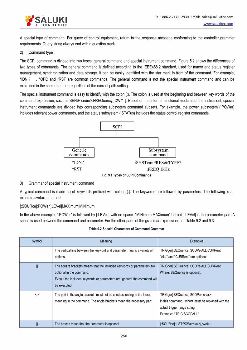
Tel: 886.2.2175 2930 Email: [email protected]
www.salukitec.com
250
A special type of command. For query of control equipment, return to the response message conforming to the controller grammarrequirements. Query string always end with a question mark.
2) Command type
The SCPI command is divided into two types: general command and special instrument command. Figure 5.2 shows the differences oftwo types of commands. The general command is defined according to the IEEE488.2 standard, used for macro and status registermanagement, synchronization and data storage. It can be easily identified with the star mark in front of the command. For example,*IDN? , *OPC and *RST are common commands. The general command is not the special instrument command and can beexplained in the same method, regardless of the current path setting.
The special instrument command is easy to identify with the colon (:). The colon is used at the beginning and between key words of thecommand expression, such as:SENS<cnum>:FREQuency[:CW?]. Based on the internal functional modules of the instrument, specialinstrument commands are divided into corresponding subsystem command subsets. For example, the power subsystem (:POWer)includes relevant power commands, and the status subsystem (:STATus) includes the status control register commands.
Fig. 9.1 Types of SCPI Commands
3) Grammar of special instrument command
A typical command is made up of keywords prefixed with colons (:). The keywords are followed by parameters. The following is anexample syntax statement:
[:SOURce]:POWer[:LEVel]MAXimum|MINimum
In the above example, ":POWer" is followed by [:LEVel], with no space. "MINimum|MAXimum" behind [:LEVel] is the parameter part. Aspace is used between the command and parameter. For the other parts of the grammar expression, see Table 9.2 and 9.3.
Table 9.2 Special Characters of Command Grammar
Symbol Meaning Examples
| The vertical line between the keyword and parameter means a variety ofoptions.
TRIGger[:SEQuence]:SCOPe ALL|CURRent"ALL" and "CURRent" are optional.
[] The square brackets means that the included keywords or parameters areoptional in the command.Even if the included keywords or parameters are ignored, the command willbe executed.
TRIGger[:SEQuence]:SCOPe ALL|CURRentWhere, SEQuence is optional.
<> The part in the angle brackets must not be used according to the literalmeaning in the command. The angle brackets mean the necessary part.
TRIGger[:SEQuence]:SCOPe <char>In this command, <char> must be replaced with theactual trigger range string.Example: ":TRIG:SCOPALL".
The braces mean that the parameter is optional. [:SOURce]:LIST:POWer<val>,<val>

Tel: 886.2.2175 2930 Email: [email protected]
www.salukitec.com
251
Example: LIST:POWer5
Table 9.3 Command Grammar
Character, Keyword and Grammar Examples
Upper-case lettering indicates the minimum set of characters requiredto execute the command.
[:SOURce]:FREQuency[:CW]?, FREQ is the short part of the command.
The lowercase character part of the command is optional. This flexibleformat is known as "flexible listening". For more information, refer tothe "Command Parameter and Response" section.
:FREQuency :FREQ,:FREQuency or FREQUENCY, both of which are correct.
If a colon is applied between two command mnemonics, the currentpath in the command tree will be moved to next layer. Refer to"Command Tree" for more information on command paths.
:TRIGger:OUTPut:POLarity?TRIGger is the keyword of the top layer of the command.
Adjacent parameters in the command should be separated withcommas. The parameters have no influence on the path layer and donot belong to the command path part.
[:SOURce]:LIST:DWELl <val>,<val>
The semicolon is used to separate two adjacent commands, with noinfluence on the current command path.
:FREQ2.5GHZ;:POW10DBM
The blank character, such as <space> or <tab>, is generally ignoredwhen not used between or in keywords. However, you must use theblank character to separate the command and parameter, with noinfluence on the current path.
":FREQuency" or ":POWer:LEVel6.2" is not allowed. ":LEVel" and "6.2" must beseparated with the space. i.e. :POWer:LEVel6.2
4) Command tree
Special instrument commands are used in most of remote control programs. To analyze this kind of command, the SCPI structureshould be similar to the file system, known as the command tree, as shown in Fig. 9.2.
Fig. 9.2 Schematic Diagram of Simplified Command Tree
The top command is the root command, referred to as the "root". Follow the specific path of the tree structure to next layer in commandanalysis. Example: :POWer:ALC:SOURce? Where, ":POWer" refers to AA, ":ALC" refers to BB, and ":SOURce" refers to GG. Thewhole command path is (:AA:BB:GG).
The command interpreter, a module of the instrument software, is dedicated to analysis of each received SCPI command. It is used todivide the command into separate command elements according to a series of rules to distinguish command tree paths. The currentcommand should be kept unchanged after analysis, so as to analyze the subsequent command more rapidly and efficiently as thesame command keyword may be used in various paths. The current command path should be set as the root after the instrument isstarted or reset (*RST).
Tel: 886.2.2175 2930 Email: [email protected]
www.salukitec.com
252
5) Command parameter and response
SCPI defines different data formats for use in program and response messages. It does this to accommodate the principle of forgivinglistening and precise talking. Refer to IEEE488.2 for more information. Forgiving listening means the command and parameter formatsare flexible.
Example: power level command of the vector network analyzer:
SOURce<cnum>:POWer<port>[:LEVel][:IMMediate][:AMPLitude]<num>,[Src] The following commands are used to set the power level:
:SOURce:POWer:LEVel:IMMediate:AMPLitude-5, :SOURce:POWer-5,
:SOUR:POW:LEV:IMM:AMP-5, :SOUR:POW-5.
Various parameter types correspond to one or more response data type(s). The numeric type of the parameter will change into thedata type in query. Response data are accurate, strictly referred to as "precise talking".
For example, if the setting is -5dBm in the power level (:SOURce:POWer?) query, the returned response data will be-5.00000000000e+000 no matter the setting command is ":SOUR:POW:LEV:IMM:AMP-5" or ":SOUR:POW- 5".
Table 9.4 SCPI Command Parameters and Response Types
Parameter type Response Data Types
Numeric Real or integer
Extended Numeric Integer
Discrete Discrete
Boolean Numeric Boolean
String String
Piece Block with Definite Length
Block of uncertain length
Non-decimal Numeric Hexadecimal system
Octal
Binary system
Numerical parameter
Special instrument commands and general commands can be expressed as numeric parameters. All kinds of common decimalcounting can be applied for reception of numeric parameters, including the plus or minus, decimal and scientific counting methods. Ifone device can only receive the specific numeric type, such as the integer, the received numeric parameter will be automaticallyrounded.
The following are examples of numeric parameters:
0 no decimal point required
100 fractional digits optional1.23 leading signs allowed
4.56e<space>3 space allowed after the E in exponential-7.89E-01 use either E or e in exponential+256 leading + allowed5 digits left of decimal point optional

Tel: 886.2.2175 2930 Email: [email protected]
www.salukitec.com
253
Extended Numeric Parameters
The numeric parameter is extended to specify the physical quantity in the majority of measurements related to special instrumentcommands. Extended numeric parameters accept all numeric parameter values and other special values as well. The extendednumeric parameters include the MAXimum and MINimum. Other special values, such as UP and DOWN, are received depending onthe analysis capability of the instrument. All effective parameters are listed in the SCPI command table.
Note: The extended numeric parameters are not applicable to general commands or STATus subsystem commands. The following areexamples of extended numeric parameters:
101 Numerical parameter1.2GHzGHz can be used as the index (E009).200MHzMHz can be used as the index (E006).
-100mV negative 100 millivolts10 degrees 10 degreeMAXimum sets parameter to largest possible valueMINimum sets parameter to smallest possible value
UP a stepper upDOWN a stepper down
Discrete Parameters
Discrete parameters are used to identify a limited number of parameters to be set. Discrete parameters use mnemonics to representeach valid setting. Similar to the programmed command mnemonics, discrete parameter mnemonics are divided into long type, shorttype and uppercase/lowercase mixed type.
Discrete parameters and commands are used together in the following examples.
:TRIGger[:SEQuence]:SOURceBUS|IMMediate|EXTernal
BUS GPIB,LAN,RS-232 triggering
IMMediate immediate triggerEXTernal external triggering
Boolean Parameters
The Boolean parameter represents one true or false binary condition, and only four possible values can be applied. The following areexamples of Boolean parameters:
ON boolean true
OFF boolean false1 boolean true0 boolean false
String Parameters
For the character string type, the ASCII character string is allowed to be transmitted as the parameter. Single and double quotes areused as delimiters. The following are examples of string parameters:
"This is Valid" "This is also Valid" "SO IS THIS"
Real Response Data
Most of test data are of real type, in the basic decimal or scientific counting format. Both formats are supported by most of advancedprogram languages.
The following are examples of real response data:
1.23E+0

Tel: 886.2.2175 2930 Email: [email protected]
www.salukitec.com
254
-1.0E+2
+1.0E+2 0.5E+0
0.23
-100.0
+100.0
0.5
Integer Response Data
Integer response data are decimal representations of integer values including signs. For status register query, integer response datawill be returned in most cases.
Examples of integer response data:
0 Signs are optional
+100 leading + allowed-100 leading + allowed256 not any decimal point
Discrete Response Data
Discrete response data are essentially similar to discrete parameters. The major difference is that only the discrete response data inthe short uppercase format are returned.
Example of discrete response data:
INTernal power leveled internallyEXTernal power leveled externallyMMHead power leveled by millimeter wave source module
Numeric Boolean Response Data
Boolean response data returns a binary numeric value of 1 or 0.
String Response Data
String response data are similar to string parameters. The main difference is that the double quotation marks instead of singlequotation marks must be used as the separator of the string response data. Double quotation marks are allowed to be embedded inthe string response data, with no character. Some examples of string response data are shown below.
"This is a string"
"one double quote inside brackets: ("")"
6) System of numeric value of command
The command value can be entered in the binary, decimal, hexadecimal or octal format. An appropriate identifier should be applied infront of the value in the binary, hexadecimal or octal format. The identifier is not required in the decimal format (default). The enteredvalue with no identifier will be saved in the decimal format. The following list shows the identifiers for the formats that require them:
#B means that the figure is a binary value.
#H means that the figure is a hexadecimal value.
#Q means that the figure is an octal value.
The following are examples of SCPI command values and identifiers for the decimal value 45:
#B101101

Tel: 886.2.2175 2930 Email: [email protected]
www.salukitec.com
255
#H2D
#Q55
In the following example, the hexadecimal value 000A is used to set the RF output power as 10dBm (or equivalent to the value in theselected unit, such as DBUV or DBUVEMF).
:POW#H000A
In the non-decimal format, the measurement unit such as DBM or mV is not used together with the value.
7) Command line structure
One command line may include multiple SCPI commands. The following methods can be applied to end the current command line:
Enter;
Enter key and EOI;
EOI and the last byte.
Commands in the command line are separated by semicolons. Commands of different subsystems begin with the colon. For example:
MMEM:COPY"Test1","MeasurementXY";:HCOP:ITEM ALL
This command line includes two commands, the first of which is the MMEM subsystem command and the second of which is theHCOP subsystem command. If adjacent commands belong to the same subsystem and the command paths are subject to partialoverlapping, the commands can be abbreviated. For example:
HCOP:ITEMALL;:HCOP:IMM
This command line includes tow commands which belong to the same level of the HCOP subsystem. The second command is startedat the level lower than the HCOP command, and the colon at the beginning of the command can be omitted. The command line can beabbreviated as follows:
HCOP:ITEMALL; IMM
9.1.4. Command Sequence and SynchronizationIEEE488.2 defines the difference of the overlapping command and continuous command.
The continuous command refers to the command sequence to be executed continuously. Generally, the speed of commandexecution is high.
The overlapping command refers the command which is not executed automatically before execution of next command. Theprocessing time of the overlapping command is generally long. The program is allowed to process other events synchronously.
Even if one command line includes multiple setting commands, commands may not be executed according to the reception sequence.In order to execute each command according to a certain sequence, all the commands must be transmitted as a separate commandline.
Example: command line including setting and query commands.
If one command line includes query commands, query results are unpredictable. The returned value will be fixed if the followingcommand is entered:
:FREQ:STAR 1 GHZ; SPAN 100;:FREQ:STAR?
Returned value: 1000000000(1GHz)
The returned value will not be fixed if the following command is entered:
:FREQ:STAR1GHz;STAR?;SPAN1000000
Tel: 886.2.2175 2930 Email: [email protected]
www.salukitec.com
256
The returned result may be the current starting frequency of the instrument before command sending, as the commands will beexecuted one by one by the host program after command messages are received. The returned result may be 1GHz in the case ofexecution after the commands are received by the host program.
Setting commands and query commands are sent separately.
General rules: setting commands and query commands should be sent in different program messages in order to ensure that thereturned results of query commands are correct.
9.1.4.1. Prevention of Overlapping Execution of Commands
In order to prevent overlapping execution of commands, multiple threads or commands can be applied, including *OPC, *OPC? or*WAI. The three commands cannot be executed until the hardware is set. The computer may be forced to wait for a certain period tosynchronize certain events in the programming process. The above methods are described below.
Use multiple threads in the control program.
Multiple threads are used to complete waiting commands and synchronize the user interface and program, that is, the command"*OPC?" is executed in each single thread, with no blockage of GUI or program threads.
The use of three commands in synchronous execution is shown in the following table.
Table 9.5 Command Grammar
Method Execution Action Programming Method
*OPC After command execution, set the operation completion bit inthe ESR register.
Set ESEBIT0;Set SREBIT5;Send the overlapping command and *OPC;Wait for the service request signal (SRQ).The service request signal means that the overlapping command hasbeen executed.
*OPC? Stop executing the current command and return to 1. Onlywhen the operation completion bit in the ESR register is set,the command will be returned, indicating that the previouscommand has been processed.
End the current command processing before executing othercommands. Directly send the command after processing of thecurrent command.
*WAI Before executing *WAI, wait for sending of all commands. Thenprocess the uncompleted commands.
End the current command processing before executing othercommands. Directly send the command after processing of thecurrent command.
9.1.5. Status Report SystemThe status report system is used to save all operation status information and error information of the current instrument. The operationstatus information and error information are respectively saved in the status register and error queue and can be inquired through theprogrammed interface.
Structure of status register organization
Application of status report system
9.1.5.1. Structure of Status Register OrganizationRegister categories are as follows:

Tel: 886.2.2175 2930 Email: [email protected]
www.salukitec.com
257
1) STB and SRE
The top register of the status report system is composed of the status byte (STB) and associated shielding register, i.e. service requestenabling register (SRE). STB is used to collect the information of registers of the lower layers and save the general working conditionsof the instrument.
2) ESR and SCPI status register
STB is used to receive the following register information:
a) Relevant values of event status registers and event status enabling (ESE) shielding registers.
b) SCPI status registers, such as STATus:OPERation and STATus:QUEStionable registers (defined by the SCPI standard),including specific operations of the instrument. All the SCPI status registers have the same internal structure (refer to "2.1.5.2Structure of SCPI Status Register" of the program control manual).
3) IST and PPE
The separate bit of SRQ and IST sign ("IndividualSTatus") is composed of the combination of all statuses of the instrument. The STBdata bit for the IST sign depends on the associated Parallel Poll Enable (PPE) Register.
4) Output buffer zone
The output buffer zone is used to save messages returned by the instrument to the controller. It does not belong to the status reportsystem, but is decisive to the MAV bit of STB. For details of the above registers, refer to "2.1.5 Status Report System" of the programcontrol manual. Refer to Fig. 9.3 for the hierarchical structure of the status register.
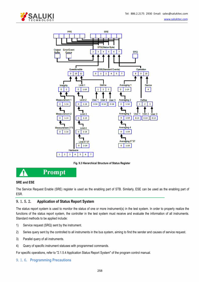
Tel: 886.2.2175 2930 Email: [email protected]
www.salukitec.com
258
Fig. 9.3 Hierarchical Structure of Status Register
SRE and ESE
The Service Request Enable (SRE) register is used as the enabling part of STB. Similarly, ESE can be used as the enabling part ofESR.
9.1.5.2. Application of Status Report SystemThe status report system is used to monitor the status of one or more instrument(s) in the test system. In order to properly realize thefunctions of the status report system, the controller in the test system must receive and evaluate the information of all instruments.Standard methods to be applied include:
1) Service request (SRQ) sent by the instrument.
2) Series query sent by the controlled to all instruments in the bus system, aiming to find the sender and causes of service request.
3) Parallel query of all instruments.
4) Query of specific instrument statuses with programmed commands.
For specific operations, refer to "2.1.5.4 Application Status Report System" of the program control manual.
9.1.6. Programming Precautions

Tel: 886.2.2175 2930 Email: [email protected]
www.salukitec.com
259
1) Initialize the instrument status before changing the setting.
For instrument setting of remote control, initialize the instrument status (sending "*RST", etc.) and then set the required status.
2) Command sequence
Generally, the setting command and query command should be transmitted separately. Otherwise, the returned value of the querycommand will change according to the current instrument operation sequence.
3) Fault response
The service request must be sent by the instrument. The controller of the test system should be programmed to guide the instrument toactively send the service request if required, so as to enable the corresponding service interruption program.
4) Error queue
The error queue instead of the status register should be inquired once the service request is processed by the controller program, soas to find more accurate causes. The queue should be always inquired in the controller program test phase to obtain the commandssent by the controller to the instrument.
9.2.Programmed Port and Configuration of Instrument
LAN
GPIB
USB
9.2.1. LAN
The programmed LAN (Local Area Network) system is configured with SICL-LAN to control AV1443 series vector network analyzer.
Use of USB master control port connector of the front panel:
The Type-A connector of the front panel is a USB master control port connector. In the AV1443 series vector network analyzer, this portis connected to the flash disc with USB1.1 interface to upgrade the software in the instrument. It can also be connected to the USBkeyboard and mouse to control the vector network analyzer. It must not be used for program control of the instrument.
9.2.1.1. Establish Connection
Connect the S3602 series vector network analyzer and external controller (computer) to LAN through network cables, as shown in Fig.9.4.
Fig. 9.4 Connection Diagram of LAN Interface

Tel: 886.2.2175 2930 Email: [email protected]
www.salukitec.com
260
Fig. 9.5 LAN Interface of Rear Panel of Instrument
9.2.1.2. Interface ConfigurationEnsure that the physical connection is smooth for remote control of the vector network analyzer by LAN. As the DHCP, domain nameaccess and WAN are not supported, the network programming of the vector network analyzer is relatively simple. In the menu shownin Fig. 9.6, set the IP address", Subnet mask" and Default gateway" to be within the subnet with the master controller.
Ensure normal physical connection of the vector network analyzer through the 10Base-TLAN or 100Base- TLAN cable.
The vector network analyzer only supports the establishment of one LAN control system and static IP address setting, and does notsupport DHCP or access to the host through the DNS and domain name server. Therefore, it is not required to modify the subnet mask.The subnet mask of the instrument should be set as the fixed value 255.255.255.0.
9.2.2. GPIB
9.2.2.1. Establish ConnectionConnect the S3602 series vector network analyzer to the external controller (computer) through the GPIB cable, as shown in Fig. 9.6.
Fig. 9.6 Connection Diagram of GPIB Interface
Fig. 9.7 GPIB Interface of Rear Panel of Instrument

Tel: 886.2.2175 2930 Email: [email protected]
www.salukitec.com
261
9.2.2.2. Interface ConfigurationWhen the system is built with the vector network analyzer, the user may need to modify the GPIB address. The default local GPIBaddress is 16. Change the GPIB address as follows:
Press [System] > [Configuration] > [GPIB address (G)...] to enter the interface shown in Fig. 9.9. Modify the GPIB address in the [LocalGPIB address] input box through the keyboard and mouse or number keys of the front panel.
9.2.3. USB
9.2.3.1. Establish Connection
Connect the S3602 series vector network analyzer to the external controller (computer) through the USB cable, as shown in Fig. 9.8.
Fig. 9.8 USB Connection Diagram
Fig. 9.9 USB Interface for Programming on Rear Panel of Instrument
9.2.3.2. Interface ConfigurationTo build a system with the vector network analyzer, the user should obtain the VID, PID and serial number of the USB address. In thedefault mode, VID is 0525, PID is 1100, and the serial number is the same as that of factory settings of the instrument. The user canalso view USB interface information by clicking [USB Test and Measurement Device (IVI) attribute] > [Details] > [Device example path]under the computer device manager of the master control computer. Generally, the VID, PID and serial number information should notbe changed under the programmed USB conditions.
9.3.Basic Programming Method of VISA InterfaceThe following example shows the basic method of instrument programming with the VISA library. Take the C++ language as theexample.
VISA library
Initialization and default state setting
Sending of setting command
Reading of measurement instrument state

Tel: 886.2.2175 2930 Email: [email protected]
www.salukitec.com
262
Reading of frequency marker
Reading of trace data
Command synchronization
9.3.1. VISA Library
VISA is a general term of the standard I/O function library and related standards. The VISA library is a set of functions which can becalled easily called. The core function can be used to control various kinds of devices, regardless of the interface type and I/O interfacesoftware operations. The function library is used to write the instrument drive program and complete command and data transmissionbetween the computer and instrument to realize the programmed control of the instrument. The instrument connection with theprogram-controlled port (LAN, USB, GPIB, RS-232, etc.) can be established by initializing the address character string ("VISA resourcestring").
The VISA library must be installed at first for remote control. The VISA library includes the transmission functions of the bottom VXI,GPIB, LAN and USB interface to facilitate direct calling. The vector network analyzer supports the following programmed interfaces:GPIB, LAN and RS-232. Such interfaces are used with the VISA library and programming languages to remotely control the vectornetwork analyzer. At present, AgilentI/OLibrary provided by Agilent is commonly used as the bottom I/O library.
Fig. 9.10 shows the relationship between the programmed interface, VISA library, programming language and vector network analyzer,with GPIB interface as an example.
Fig. 9.10 Programming Software and Hardware Layer
9.3.2. Initialization and Default State SettingInitialize the VISA resource manager at the beginning of programming. Open the VISA library and establish the communicationconnection between the VISA library and instrument. Specific steps are as follows.
9.3.2.1. Generation of Global VariablesAt first, generate global variables to be called by other program modules, such as instrument handle variables. The following globalvariables are included in the program example.
ViSession analyzer;
ViSession defaultRM;

Tel: 886.2.2175 2930 Email: [email protected]
www.salukitec.com
263
Const char analyzerString [VI_FIND_BUFLEN] = "GPIB0::16::INSTR";
Const analyzerTimeout = 10000;
The constant analyzerString refers to the instrument descriptor, “GPIB0" refers to the controller, and "16" refers to the instrumentconnected to the controller. Assuming that the instrument is connected LAN, the IP address is "192.168.1.1" and the port number is"1024", the variable is:
Const char analyzerString [VI_FIND_BUFLEN] = "TCPIPO::192.168.1.1::1024::SOCKET";
9.3.2.2. Controller InitializationThe following example shows how to establish the communication connection between the VISA library and instrument (with thespecified descriptor).
//Controller initialization: open the default resource manager and return the instrument handle to the analyzer.
void InitController()
ViStatus status;
status = viOpenDefaultRM(&defaultRM);
status = viOpen(defaultRM, analyzerString, VI_NULL, VI_NULL, &analyzer);
9.3.2.3. Instrument Initialization
/*************************************************************************/
The following example shows the initialization of the default instrument state and clearing of the status register. "\n" refers to theterminator. The character string of each command should be ended with ‘\n‘. This will not be described later.
/*************************************************************************/
void InitDevice()
ViStatus status; long retCnt;
status = viWrite(analyzer, "*CLS\n", 5, &retCnt); //reset status register
status = viWrite(analyzer, "*RST\n", 5, &retCnt); //reset instrument
9.3.2.4. Query of Instrument Measurement Information/*************************************************************************
/ The following example shows all measurements, windows and tracks defined at present.
/*************************************************************************/
void QueryMesaurement()
ViStatus status; long retCnt;
char rd_Buf_CW[VI_READ_BUFLEN]; // #define VI_READ_BUFLEN 20 char rd_Buf_LVL[VI_READ_BUFLEN];
// query all measurements of Channel 1

Tel: 886.2.2175 2930 Email: [email protected]
www.salukitec.com
264
status = viWrite(analyzer, ": CALC:PAR:CAT?\n", 15, &retCnt); Sleep(10);
status = viRead(analyzer, rd_Buf_CW, 50, &retCnt);
// query all windows
status = viWrite(analyzer, ": DISP:CAT?\n", 11, &retCnt); Sleep(10);
status = viRead(analyzer, rd_Buf_CW, 20, &retCnt);
// query all tracks of Window 1
status = viWrite(analyzer, ": DISP:WIND1:CAT?\n", 18, &retCnt); Sleep(10);
status = viRead(analyzer, rd_Buf_CW, 20, &retCnt);
9.3.3. Sending of Setting Command
9.3.3.1. Setting of sweep Parameters /
*************************************************************************/
The following example shows how to set the sweep parameters of S3602 series vector network analyzers. /
*************************************************************************/
void SweepSettings()
ViStatus status; long retCnt;
// selection of measurement
status = viWrite(analyzer, ":CALC:PAR:SEL „CH1_WIN1_LINE1‟ \n", 50,&retCnt);
// set the scanning type as linear sweep
status = viWrite(analyzer, ":SENSe1:SWEep:TYPE LIN\n", 30, &retCnt);
// set the IF bandwidth as 3KHz
status = viWrite(analyzer, " :SENSe1:BANDwidth 3000\n", 30, &retCnt);
// set the starting frequency as 1GHz and ending frequency as 10GHz status = viWrite(analyzer, ":SENS:FREQ:STAR 1e9\n", 30,&retCnt); status = viWrite(analyzer, ":SENS:FREQ:STOP 1e10\n", 30, &retCnt);
// set the number of sweep points as 401
status = viWrite(analyzer, ":SENSe1:SWEep:POINts 401\n", 30, &retCnt);
// automatic setting of sweep time
status = viWrite(analyzer, ":SENSe1:SWEep:TIME:AUTO ON\n", 40, &retCnt);
// set the output power as -10dBm
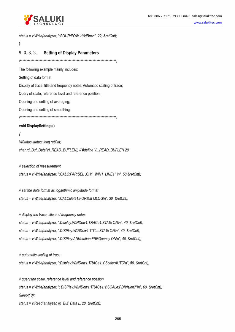
Tel: 886.2.2175 2930 Email: [email protected]
www.salukitec.com
265
status = viWrite(analyzer, ":SOUR:POW -10dBm\n", 22, &retCnt);
9.3.3.2. Setting of Display Parameters/*************************************************************************/
The following example mainly includes:
Setting of data format;
Display of trace, title and frequency notes; Automatic scaling of trace;
Query of scale, reference level and reference position;
Opening and setting of averaging;
Opening and setting of smoothing.
/*************************************************************************/
void DisplaySettings()
ViStatus status; long retCnt;
char rd_Buf_Data[VI_READ_BUFLEN]; // #define VI_READ_BUFLEN 20
// selection of measurement
status = viWrite(analyzer, ":CALC:PAR:SEL „CH1_WIN1_LINE1‟ \n", 50,&retCnt);
// set the data format as logarithmic amplitude format
status = viWrite(analyzer, ":CALCulate1:FORMat MLOG\n", 30, &retCnt);
// display the trace, title and frequency notes
status = viWrite(analyzer, ":Display:WINDow1:TRACe1:STATe ON\n", 40, &retCnt);
status = viWrite(analyzer, ":DISPlay:WINDow1:TITLe:STATe ON\n", 40, &retCnt);
status = viWrite(analyzer, ":DISPlay:ANNotation:FREQuency ON\n", 40, &retCnt);
// automatic scaling of trace
status = viWrite(analyzer, ":Display:WINDow1:TRACe1:Y:Scale:AUTO\n", 50, &retCnt);
// query the scale, reference level and reference position
status = viWrite(analyzer, ": DISPlay:WINDow1:TRACe1:Y:SCALe:PDIVision?"\n", 60, &retCnt);
Sleep(10);
status = viRead(analyzer, rd_Buf_Data L, 20, &retCnt);
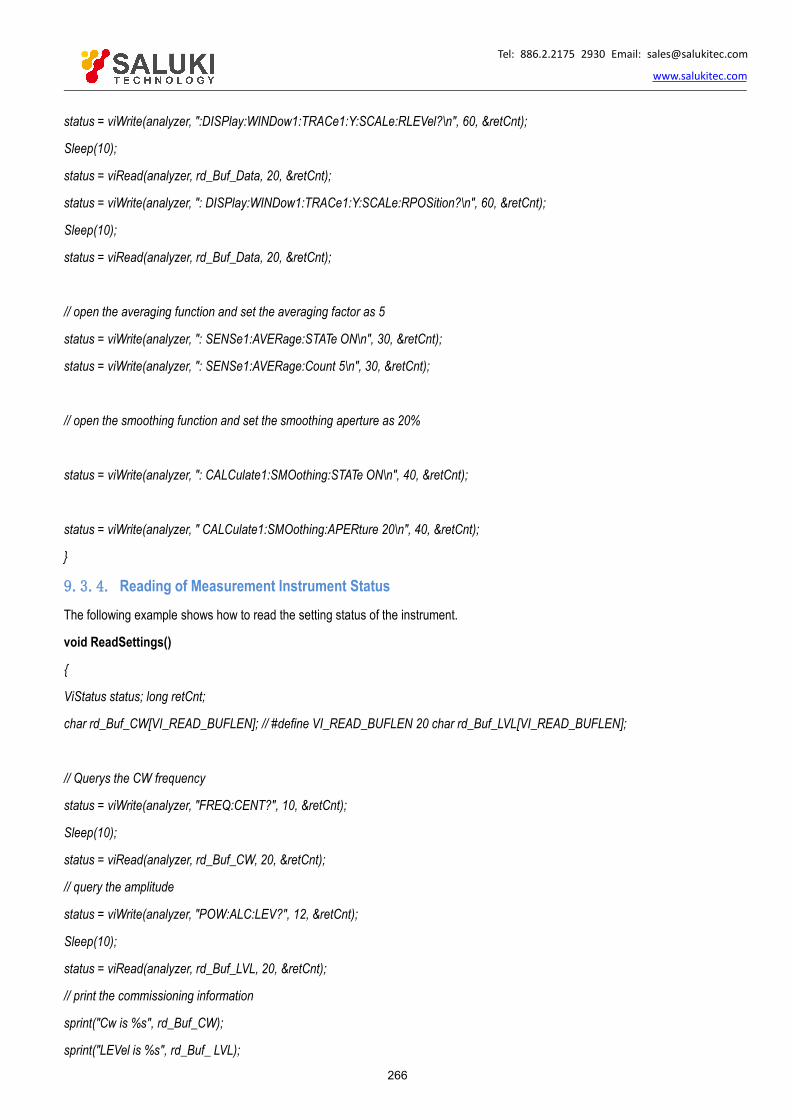
Tel: 886.2.2175 2930 Email: [email protected]
www.salukitec.com
266
status = viWrite(analyzer, ":DISPlay:WINDow1:TRACe1:Y:SCALe:RLEVel?\n", 60, &retCnt);
Sleep(10);
status = viRead(analyzer, rd_Buf_Data, 20, &retCnt);
status = viWrite(analyzer, ": DISPlay:WINDow1:TRACe1:Y:SCALe:RPOSition?\n", 60, &retCnt);
Sleep(10);
status = viRead(analyzer, rd_Buf_Data, 20, &retCnt);
// open the averaging function and set the averaging factor as 5
status = viWrite(analyzer, ": SENSe1:AVERage:STATe ON\n", 30, &retCnt);
status = viWrite(analyzer, ": SENSe1:AVERage:Count 5\n", 30, &retCnt);
// open the smoothing function and set the smoothing aperture as 20%
status = viWrite(analyzer, ": CALCulate1:SMOothing:STATe ON\n", 40, &retCnt);
status = viWrite(analyzer, " CALCulate1:SMOothing:APERture 20\n", 40, &retCnt);
9.3.4. Reading of Measurement Instrument Status
The following example shows how to read the setting status of the instrument.
void ReadSettings()
ViStatus status; long retCnt;
char rd_Buf_CW[VI_READ_BUFLEN]; // #define VI_READ_BUFLEN 20 char rd_Buf_LVL[VI_READ_BUFLEN];
// Querys the CW frequency
status = viWrite(analyzer, "FREQ:CENT?", 10, &retCnt);
Sleep(10);
status = viRead(analyzer, rd_Buf_CW, 20, &retCnt);
// query the amplitude
status = viWrite(analyzer, "POW:ALC:LEV?", 12, &retCnt);
Sleep(10);
status = viRead(analyzer, rd_Buf_LVL, 20, &retCnt);
// print the commissioning information
sprint("Cw is %s", rd_Buf_CW);
sprint("LEVel is %s", rd_Buf_ LVL);
Tel: 886.2.2175 2930 Email: [email protected]
www.salukitec.com
267
9.3.5. Reading of Frequency Marker/*************************************************************************/
The following example shows how to read the frequency scale information.
/*************************************************************************/
void ReadMarker ()
ViStatus status;
long retCnt;
char rd_Buf_Marker[VI_READ_BUFLEN]; // #define VI_READ_BUFLEN 20
// open the frequency marker 1 and query the frequency marker peak (frequency and amplitude)
status = viWrite(analyzer, ":CALC:MARKER ON;MARKER: FUNCtion:EXECute MAXimum\n", 25, &retCnt);
// read the X-axis information
status = viWrite(analyzer, ":CALC:MARK:X?; ", 15, &retCnt);
status = viRead(analyzer, rd_Buf_Marker, 30, &retCnt);
// read the Y-axis coordinate information
status = viWrite(analyzer, ":CALC:MARK:Y?; ", 15, &retCnt);
status = viRead(analyzer, rd_Buf_Marker, 30, &retCnt);
9.3.6. Reading of trace Data /*************************************************************************/
The following example shows how to read the trace data of the vector network analyzer. /
*************************************************************************/
void QueryData ()
ViStatus status;
long retCnt = 0;
int points= 0
// #define VI_READ_BUFLEN 1000000
char rd_Buf_BigData[VI_READ_DATABUFLEN];
char rd_Buf_Data[VI_READ_BUFLEN]; // #define VI_READ_BUFLEN 20
// selection of measurement

Tel: 886.2.2175 2930 Email: [email protected]
www.salukitec.com
268
status = viWrite(analyzer, ":CALCulate:PARameter:SELect ' CH1_WIN1_LINE1'\n", 25,&retCnt);
// obtain the number of sweep point
status = viWrite(analyzer, ":SENSe1:SWEep:POIN?\n", 15, &retCnt);
status = viRead(analyzer, rd_Buf_Data, 30, &retCnt);
points = atoi(rd_Buf_Data);
// sweep once
status = viWrite(analyzer, ":SENSe1:SWEep:GROups:COUNt 1\n",30, &retCnt);
status = viWrite(analyzer, ":SENS:SWE:MODE GROups\n",30, &retCnt);
// sending and reading of data command. Here the data format is original data, divided into the real part and imaginary part. Thereturned character//string format is: "real part of the first point, imaginary part of the first point, real part of the second point, imaginarypart of the second point..."
status = viWrite(analyzer, ": CALCulate:DATA? SDATA\n",30, &retCnt);
status = viRead(analyzer, rd_Buf_BigData, VI_READ_BUFLEN, &retCnt);
9.3.7. Command SynchronizationThe method of command synchronization is introduced below, taking the sweep process as an example.
void SweepSync()
ViStatus status;
long retCnt;
ViEventType etype;
ViEvent eevent;
int stat;
char OpcOk [2];
/*********************************************************************/
/* Command INITiate[:IMMediate] start single sweep ( closed in continuous scanningINIT:CONT OFF)*/
* Execute next command of command buffer zone after single sweep */
*********************************************************************/
status = viWrite(analyzer, "INIT:CONT OFF", 13, &retCnt);
// Method 1 of waiting for ending of sweep: use *WAI
status = viWrite(analyzer, "ABOR;INIT:IMM;*WAI", 18, &retCnt);
// Method 2 of waiting for ending of sweep: use *OPC?

Tel: 886.2.2175 2930 Email: [email protected]
www.salukitec.com
269
status = viWrite(analyzer, "ABOR;INIT:IMM; *OPC?", 20, &retCnt);
status = viRead(analyzer, OpcOk, 2, &retCnt); //Wait for*OPC and return to "1"
// Method 3 of waiting for ending of sweep: use *OPC
// To enable GPIB service request, set "Disable Auto Serial Poll" as "yes"
status = viWrite(analyzer, "*SRE 32", 7, &retCnt);
status = viWrite(analyzer, "*ESE 1", 6, &retCnt); // enable service request ESR
// set event enabling bit to complete operation
status = viEnableEvent(analyzer, VI_EVENT_SERVICE_REQ, VI_QUEUE, VI_NULL);
// enable SRQ event
status = viWrite(analyzer, "ABOR;INIT:IMM;*OPC", 18, &retCnt);
// start sweep synchronously with OPC
status = viWaitOnEvent(analyzer, VI_EVENT_SERVICE_REQ, 10000, &etype, &eevent)
// wait for service request
status = viReadSTB(analyzer, &stat);
status = viClose(eevent); // close event handle
// prohibit SRQ event
status = viDisableEvent(analyzer, VI_EVENT_SERVICE_REQ, VI_QUEUE);
// main program continues……
9.4.I/O Library
9.4.1. Overview of I/O LibraryThe I/O library is a library of pre-written software programs for the instrument, known as the instrument drive program, i.e. instrumentdriver. It is an intermediate software layer between the computer and instrument hardware equipment. It is composed of the functionlibrary, utility program, tool kit, etc., and is a set of software code modules. This set corresponds to a series of planned operations,such as instrument configuration, reading, writing, triggering, etc. It is installed the computer and used as a connecting bridge and linkbetween the computer and instrument. With the easy-to-program high-level modular library, the user does not need to the complexspecial low-level programming protocol for the specific instrument. It is key to use the instrument driver to rapidly develop the testmeasurement application.
From the functional perspective, one general instrument driver is composed of five parts: functional body, interactive developerinterface, program developer interface, subprogram interface and I/O interface, as shown in Fig. 9.11.
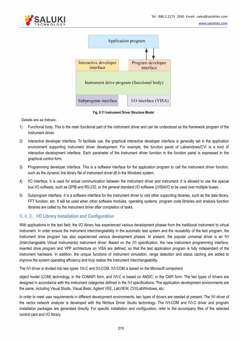
Tel: 886.2.2175 2930 Email: [email protected]
www.salukitec.com
270
Fig. 9.11 Instrument Driver Structure Model
Details are as follows:
1) Functional body. This is the main functional part of the instrument driver and can be understood as the framework program of theinstrument driver.
2) Interactive developer interface. To facilitate use, the graphical interactive developer interface is generally set in the applicationenvironment supporting instrument driver development. For example, the function panel of Labwindows/CVI is a kind ofinteractive development interface. Each parameter of the instrument driver function in the function panel is expressed in thegraphical control form.
3) Programming developer interface. This is a software interface for the application program to call the instrument driver function,such as the dynamic link library file of instrument driver.dll in the Windows system.
4) I/O interface. It is used for actual communication between the instrument driver and instrument. It is allowed to use the specialbus I/O software, such as GPIB and RS-232, or the general standard I/O software ()VISAI/O to be used over multiple buses.
5) Subprogram interface. It is a software interface for the instrument driver to visit other supporting libraries, such as the data library,FFT function, etc. It will be used when other software modules, operating systems, program code libraries and analysis functionlibraries are called by the instrument driver after completion of tasks.
9.4.2. I/O Library Installation and ConfigurationWith applications in the test field, the I/O library has experienced various development phases from the traditional instrument to virtualinstrument. In order ensure the instrument interchangeability in the automatic test system and the reusability of the test program, theinstrument drive program has also experienced various development phases. At present, the popular universal driver is an IVI(Interchangeable Virtual Instruments) instrument driver. Based on the IVI specification, the new instrument programming interface,inserted drive program and VPP architecture on VISA are defined, so that the test application program is fully independent of theinstrument hardware. In addition, the unique functions of instrument simulation, range detection and status caching are added toimprove the system operating efficiency and truly realize the instrument interchangeability.
The IVI driver is divided into two types: IVI-C and IVI-COM. IVI-COM is based on the Microsoft component
object model (COM) technology, in the COMAPI form, and IVI-C is based on ANSIC, in the CAPI form. The two types of drivers aredesigned in accordance with the instrument categories defined in the IVI specifications. The application development environments arethe same, including Visual Studio, Visual Basic, Agilent VEE, LabVIEW, CVI/LabWindows, etc.
In order to meet user requirements in different development environments, two types of drivers are needed at present. The IVI driver ofthe vector network analyzer is developed with the Nimbus Driver Studio technology. The IVI-COM and IVI-C driver and programinstallation packages are generated directly. For specific installation and configuration, refer to the accompany files of the selectedcontrol card and I/O library.

Tel: 886.2.2175 2930 Email: [email protected]
www.salukitec.com
271
The installed IVI driver is divided into the IVI inherent function group and instrument function group (basic function group and extendedfunction group). For specific functional classification, functions and attribute details, refer to the help file of the driver.
Port configuration and I/O library installation:
Before controlling the vector network analyzer with a computer, check whether the necessary port and I/O library are properly installedand configured.
Use of I/O library:
If the accompanying IVI-COM/C drive program installation package is installed, the function panel, help file and drive function exampleprograms will be installed automatically to facilitate development and integration of the programmed functions.
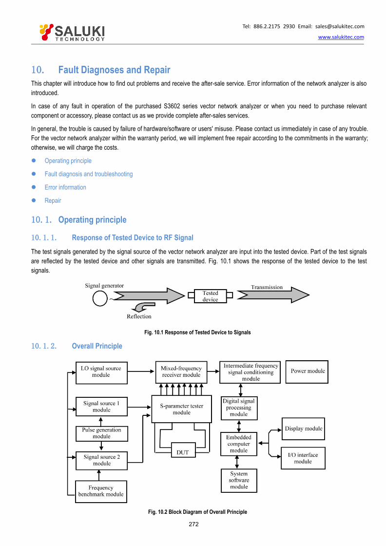
Tel: 886.2.2175 2930 Email: [email protected]
www.salukitec.com
272
10. Fault Diagnoses and RepairThis chapter will introduce how to find out problems and receive the after-sale service. Error information of the network analyzer is alsointroduced.
In case of any fault in operation of the purchased S3602 series vector network analyzer or when you need to purchase relevantcomponent or accessory, please contact us as we provide complete after-sales services.
In general, the trouble is caused by failure of hardware/software or users' misuse. Please contact us immediately in case of any trouble.For the vector network analyzer within the warranty period, we will implement free repair according to the commitments in the warranty;otherwise, we will charge the costs.
Operating principle
Fault diagnosis and troubleshooting
Error information
Repair
10.1. Operating principle
10.1.1. Response of Tested Device to RF SignalThe test signals generated by the signal source of the vector network analyzer are input into the tested device. Part of the test signalsare reflected by the tested device and other signals are transmitted. Fig. 10.1 shows the response of the tested device to the testsignals.
Fig. 10.1 Response of Tested Device to Signals
10.1.2. Overall Principle
Fig. 10.2 Block Diagram of Overall Principle

Tel: 886.2.2175 2930 Email: [email protected]
www.salukitec.com
273
S3602 series vector network analyzers are intelligent test instrument designed based on the modular concept, with the embeddedindustrial computer module as the control center. The design concept includes the "embedded computer hardware platform based onthe multi-processor + test module", realizing the perfect combination of the test instrument and industrial computer. The test controlsoftware with the Windows operating system can make the human-machine interface of the instrument more friendly and the operationmore convenient. The block diagram of modular design of the instrument is shown in Fig. 10.2. The system mainly includes the LOsignal source module, signal source module 1, signal source module 2, frequency benchmark module, S-parameter tester module,mixed- frequency receiver module, IF signal processing module, digital signal processing module, embedded computer module, powersupply module, display module, I/O interface module, software module, etc.
The frequency benchmark module is locked to the internal or external 10MHz reference signal to produce the locking reference signalfor the LO source and signal source and the synchronization signal for the whole instrument.
The LO signal source module and stimulus signal source module are locked to the reference signal output by the frequencybenchmark module, to produce the required LO signal and RF signal through the switching frequency doubling device, subbandbandpass filter and automatic level control circuit (ALC).
The S-parameter tester module is a signal separator to separate the incident signal, reflected signal and transmitted signal of thetested device.
In the mixed-frequency receiver module, the incident, reflected and transmitted signals including the amplitude and phase informationof the tested device are mixed with LO signals, and the generated IF signals are transmitted to the IF signal conditioning module forfurther processing.
The IF signals are conditioned by the IF signal conditioning module to meet the requirements of the digital signal processing modulefor IF signals.
In the digital signal processing module, the analog IF signals are transformed into digital signals, and then the digital signals areprocessed to obtain the amplitude and phase information of the tested device. Measurement results are transmitted to the main CPUthrough the high-speed PCI bus.
The system test control module run on the embedded PC platform is used to transform the amplitude and phase information of thetested device into various formats, and the results are transmitted to the display module. In addition, the system software is also usedfor management of various interfaces and scheduling of various processes of the instrument.
10.2. Fault Diagnosis and Troubleshooting
Fault diagnosis and guidance
This section aims to guide simple judgment and disposal of faults of S3602 series vector network analyzers. If necessary, provideaccurate feedback to the manufacturer to solve problems as soon as possible.
If any information appears in the status indication zone of the user interface, view [Help] > [Error information] > [View error log] to knowspecific information.
System problems
Curve display anomaly
sweep problems
Display problems
Response failure of front panel keys
Menu failure

Tel: 886.2.2175 2930 Email: [email protected]
www.salukitec.com
274
10.2.1. System Problems
10.2.1.1. The standby light is not ON.Check whether the 220V AC power input of the network analyzer is normal. The allowable maximum deviation is 220V±10%. If thedeviation is too large or small, the instrument may not work normally. In case of abnormality, check external wires for any failure; poweron the instrument again and restart it after trouble-shooting. If the 220V AC power input is normal, check whether the power switch onthe rear panel of the instrument is turned on. Under
normal conditions, the power switch should be in the "丨" state. If the fault is caused by the power supply of the instrument, send theinstrument to the manufacturer for repair.
10.2.1.2. The system cannot be enabled after start-up.If the system cannot be enabled after start-up, first check whether the hard disc on the rear panel is loose. If the hard disc is loose,tighten the fixing screw or pull out and reinsert the hard disc. If the hard disc is not loose, recover the system. For specific steps, referto "3.1.2.1 System Recovery of Network Analyzer".
10.2.1.3. The network analyzer software cannot be used after start-up.
If the network analyzer software cannot be used after start-up and system enabling, double-click the desktop icon( )of the vectornetwork analyzer or press the [Reset] key on the front panel or click [Start] > [Programs] > [Vector network analyzer] to start theprogram. If the software can be started smoothly, install the antivirus software to kill viruses and restart the instrument. If the softwarecannot be started automatically, download the vector network analyzer program and double-lick the vector network analyzer installationprogram in the root directory of Disc D or E. Reinstall the vector network analyzer program .
10.2.2. Curve Display Anomaly
The curve display anomaly is caused for various reasons. At first, check whether the user reset state is saved. Click [System] >[Custom user reset state] in the menu bar to open the [Custom user state] window. Remove the tick in the check box in front of "Savefinal state as user reset state" and "Enable user reset state". Click OK to close the [Custom user state] window. Press [Reset] on thefront panel. The S11 curve should be near 0 if the port is not connected with any load.
If the curve is still abnormal after the above methods are applied, contact our technical support personnel for solutions.
10.2.3. Sweep Problems
10.2.3.1. Sweep seems stopped.
The open-circuit curve of the port seems no sweep in the reset state. This is caused by high stability and sweep speed of the vectornetwork analyzer. Click [Stimulus] > [Scanning] > [Sweep time], enter 20 and press ENTER. Then you can see the sweep marker.
10.2.3.2. sweep is stopped.
Check whether the instrument is in the HOLD state. If the instrument is in the HOLD state, modify the trigger mode and press[Stimulus] > [Trigger] > [Continuous sweep] or open the [Trigger] dialog box and set the automatic trigger mode.
10.2.4. The white sweep marker is in the lower part of the screen.Both ports should be scanned for correction after full 2-port calibration. If only the trace with the stimulus source on Port 1 is displayed,the white marker will appear in the lower part of the screen to sweep Port 2. This is a normal sweep state and no change is required.
10.2.5. Display ProblemsIf the display window is blocked by the task bar, right-click the task bar, click [Attribute], tick "Automatic hide task bar" and click OK toclose the dialog box. In this case, the task bar will be automatically hided and the test window will not be blocked.
10.2.6. No Response of Front Panel Keys
Tel: 886.2.2175 2930 Email: [email protected]
www.salukitec.com
275
In case of no response of front panel keys, which is caused by damage of the instrument drive program, download the vector networkanalyzer and reinstall it. For specific steps, refer to "3.1.2.2 Updating of Network Analyzer Program". Select the "Complete" installationtype and reinstall the drive program. If the problem still exists, recover the system. For specific steps, refer to "3.1.2.1 SystemRecovery of Network Analyzer".
10.2.7. Menu Failure
In case of menu failure, at first check whether the GPIB status at the bottom of the window is LOCAL. If the program-controlled state isenabled, press the [Macro/Local] key on the front panel or connect the keyboard and press [Esc] to recover the local state.
10.3. Error InformationAny error will be reported in the error queue of SCPI (remote control interface) and the error queue displayed on the front panel. Twoqueues are displayed and processed independently. For details of the error queue of the front panel, refer to the User Manual.
If the SCPI (remote interface) error queue is used for access to messages, the error number and <Description> in the error queue willbe displayed on the host terminal.
The error information of the vector network analyzer can be displayed and recorded in the error file. The user can select to select ornot to select the error information.
10.3.1. Local Error Information
10.3.1.1. Viewing of Error Information By interface operation:
The error or warning prompt information in the test interface of the vector network analyzer in operation indicates operation orhardware problems. All prompt, warning and error events in operation are recorded in the error log of the vector network analyzer.Using the error log, the user can view the date, time, etc. of the concerned prompt, warning and error details, and click "Help" forfurther information. Only one piece of error information can be displayed at the specific time. As the problems may occur at the sametime, the following operations can help to view all the error prompt information:
Step 1: press [Help] > [Error information] > [View error log]. The [Error log] window will pop up.
Step 2: prompt information will be displayed in the window.
Step 3: browse the error information with the mouse and close the dialog window.
Step 4: click [Clear error list] to clear historical error information.
10.3.1.2. Description of Error Information
If any error is detected in measurement with the vector network analyzer, the warning or error information will be displayed in the testinterface. In the default mode, error information will be displayed for a certain period of time. The user can keep error informationdisplayed on the screen until "OK" is pressed, or select not to display the error information. When the error information is displayed onthe screen, you can click [Help] for further help information.
Table 10.1 Level Distinguishing with Fonts and Colors
Color Warning Level Description
Red Error Error in measurement, such as failure caused by data loss or improper setting.
Blue Warning Irregular operation in measurement, such as failure of measurement as a result of mismatch of the instrument settingand displayed result or temporary disconnection with the external device.
Black Prompt Step setting or measurement information.
10.3.2. Program Error Information
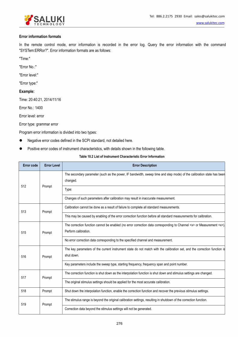
Tel: 886.2.2175 2930 Email: [email protected]
www.salukitec.com
276
Error information formats
In the remote control mode, error information is recorded in the error log. Query the error information with the command"SYSTem:ERRor?". Error information formats are as follows:
"Time:"
"Error No.:"
"Error level:"
"Error type:"
Example:
Time: 20:40:21, 2014/11/16
Error No.: 1400
Error level: error
Error type: grammar error
Program error information is divided into two types:
Negative error codes defined in the SCPI standard, not detailed here.
Positive error codes of instrument characteristics, with details shown in the following table.
Table 10.2 List of Instrument Characteristic Error Information
Error code Error Level Error Description
512 Prompt
The secondary parameter (such as the power, IF bandwidth, sweep time and step mode) of the calibration state has beenchanged.
Type:
Changes of such parameters after calibration may result in inaccurate measurement.
513 PromptCalibration cannot be done as a result of failure to complete all standard measurements.
This may be caused by enabling of the error correction function before all standard measurements for calibration.
515 Prompt
The correction function cannot be enabled (no error correction data corresponding to Channel <x> or Measurement <x>).Perform calibration.
No error correction data corresponding to the specified channel and measurement.
516 Prompt
The key parameters of the current instrument state do not match with the calibration set, and the correction function isshut down.
Key parameters include the sweep type, starting frequency, frequency span and point number.
517 PromptThe correction function is shut down as the interpolation function is shut down and stimulus settings are changed.
The original stimulus settings should be applied for the most accurate calibration.
518 Prompt Shut down the interpolation function, enable the correction function and recover the previous stimulus settings.
519 PromptThe stimulus range is beyond the original calibration settings, resulting in shutdown of the correction function.
Correction data beyond the stimulus settings will not be generated.
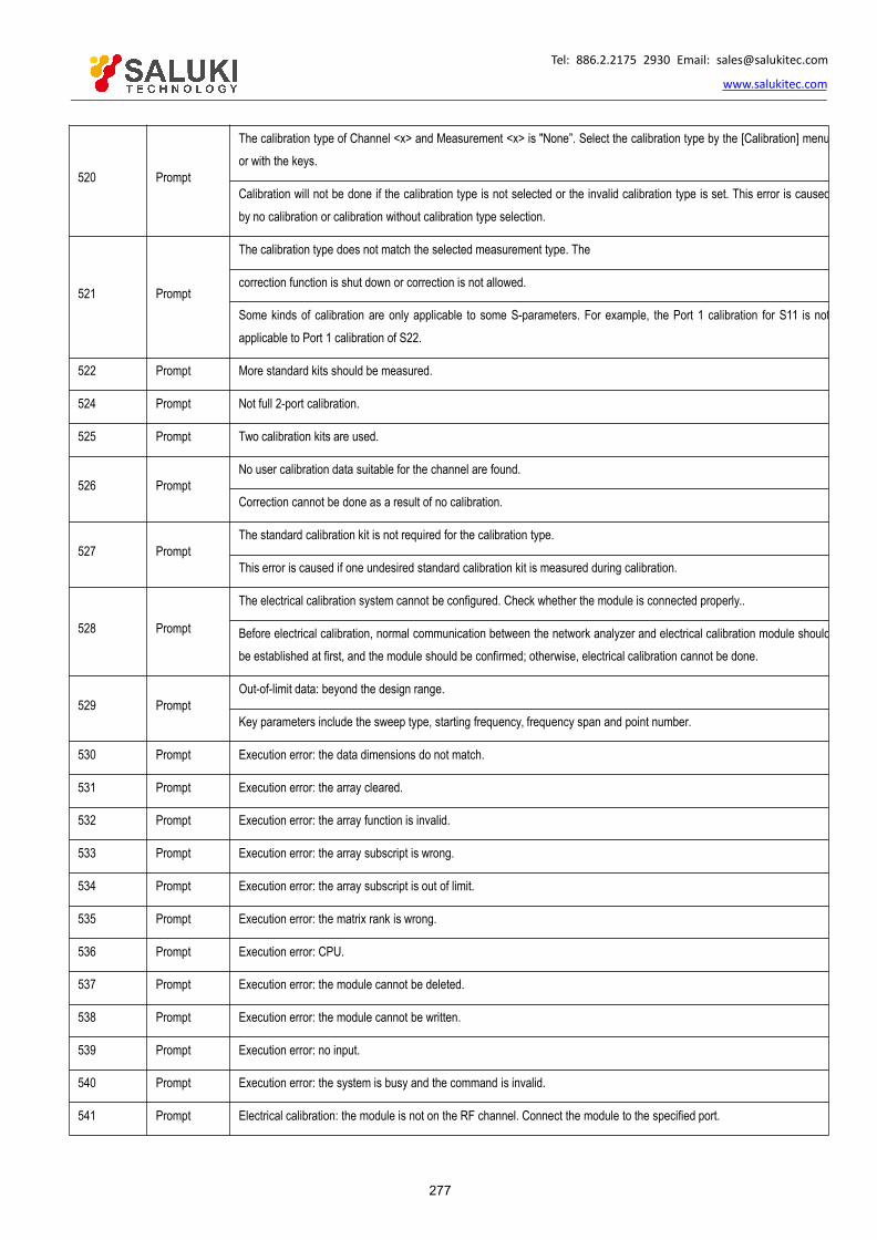
Tel: 886.2.2175 2930 Email: [email protected]
www.salukitec.com
277
520 Prompt
The calibration type of Channel <x> and Measurement <x> is "None”. Select the calibration type by the [Calibration] menuor with the keys.
Calibration will not be done if the calibration type is not selected or the invalid calibration type is set. This error is causedby no calibration or calibration without calibration type selection.
521 Prompt
The calibration type does not match the selected measurement type. The
correction function is shut down or correction is not allowed.
Some kinds of calibration are only applicable to some S-parameters. For example, the Port 1 calibration for S11 is notapplicable to Port 1 calibration of S22.
522 Prompt More standard kits should be measured.
524 Prompt Not full 2-port calibration.
525 Prompt Two calibration kits are used.
526 PromptNo user calibration data suitable for the channel are found.
Correction cannot be done as a result of no calibration.
527 PromptThe standard calibration kit is not required for the calibration type.
This error is caused if one undesired standard calibration kit is measured during calibration.
528 Prompt
The electrical calibration system cannot be configured. Check whether the module is connected properly..
Before electrical calibration, normal communication between the network analyzer and electrical calibration module shouldbe established at first, and the module should be confirmed; otherwise, electrical calibration cannot be done.
529 PromptOut-of-limit data: beyond the design range.
Key parameters include the sweep type, starting frequency, frequency span and point number.
530 Prompt Execution error: the data dimensions do not match.
531 Prompt Execution error: the array cleared.
532 Prompt Execution error: the array function is invalid.
533 Prompt Execution error: the array subscript is wrong.
534 Prompt Execution error: the array subscript is out of limit.
535 Prompt Execution error: the matrix rank is wrong.
536 Prompt Execution error: CPU.
537 Prompt Execution error: the module cannot be deleted.
538 Prompt Execution error: the module cannot be written.
539 Prompt Execution error: no input.
540 Prompt Execution error: the system is busy and the command is invalid.
541 Prompt Electrical calibration: the module is not on the RF channel. Connect the module to the specified port.

Tel: 886.2.2175 2930 Email: [email protected]
www.salukitec.com
278
The RF channel is not connected to the electrical calibration module, and no signal is found in the correspondingcalibration measurement.
542 PromptExecution error: no space for new calibration kit. Delete one calibration kit. Key parameters include the sweep type,starting frequency, frequency span and point number.
543 Prompt Execution error: the space is not enough.
544 Prompt Execution error: other matrix errors.
545 Prompt Execution error: unequal rank.
546 Prompt Execution error: few constant ranks.
547 Prompt Execution error: few variable ranks.
548 Prompt Perform pre-calibration.
549 Prompt Execution error: bug in the dynamic library of electrical calibration drivers or invalid module number.
550 Prompt Execution error: accidental error from the electrical calibration driver.
551 Prompt Execution error: error of the built-in driver.
552 Prompt Hardware error: failure of access to the electrical calibration module.
553 Prompt Hardware error: failure to release the LPT port. Restart the instrument.
554 Prompt Hardware error: error of the vector network analyzer.
555 Prompt Hardware error: failure to read enough data from the electrical calibration module.
556 Prompt Suspension of the master control computer.
557 Prompt Suspension of user operation.
558 Prompt Out-of-limit memory.
559 Prompt Ended query: the message is abandoned.
560 Prompt Unfinished query: incomplete application message.
561 Prompt Unfinished query: no content.
562 Prompt Queue overflow.
563 Prompt Setting conflict: requiring the additional standard calibration kit.
564 Prompt Setting conflict: the adapter cannot be calibrated.
565 Prompt Setting conflict: the command queue is subject to overflow.
566 Prompt Setting conflict: calibration is stopped, as a result of changes of analyzer settings.
567 Prompt Setting conflict: calibration is not done.
568 Prompt Setting conflict: the specified GPIB board cannot be found.
569 Prompt Setting conflict: gpib32.dll cannot be found/installed.
570 Prompt Setting conflict: sicl32.dll cannot be found/installed.

Tel: 886.2.2175 2930 Email: [email protected]
www.salukitec.com
279
571 Prompt Setting conflict: the network analyzer cannot be initialized (wrong address?).
572 Prompt Setting conflict: the print port drive program or USB-driven dynamic library cannot be loaded.
573 Prompt Setting conflict: the calibration canning mode is invalid.
574 Prompt Setting conflict: the calibration type is invalid.
575 Prompt Setting conflict: calibration is invalid.
576 Prompt Setting conflict: the specified GPIB board number is invalid.
577 Prompt Setting conflict: the specified GPIB board type is invalid.
578 Prompt Setting conflict: the module state is invalid.
579 Prompt Setting conflict: the state is invalid.
580 Prompt Setting conflict: the LPT port must be 1-4.
581 Prompt The electrical calibration system cannot be configured. Check whether the module is connected properly.
582 Prompt Setting conflict: the specified LPT port does not exist.
583 Prompt Setting conflict: use the frequency domain in calibration.
584 Prompt Setting conflict: use the step sweep type in calibration.
585 Prompt Setting conflict: the analyzer address must be 0-30.
586 Prompt Setting conflict: wrong print port driver or USB-driven dynamic library.
587 Prompt Grammar error: the ECAL: DELAY must include two digits.
588 Prompt Grammar error: incorrect grammar.
589 Prompt Grammar error: unknown command.
590 Prompt The module port on the RF channel is wrong.
591 Prompt The module does not conform to the requirements described by the user.
592 PromptThe source power calibration data corresponding to the current measurement channel and source port are not found.
Try to enable the source power calibration function, but no calibration data are found.
593 Prompt
Failure of source power calibration sweep or correction of the channel and source port corresponding to the currentmeasurement.
Try to enable the source power calibration function, but calibration data are not complete.
594 Prompt Reserved.
595 Prompt Reserved.
596 PromptThe calibration function is enabled, but the calibration power is changed in source power calibration of Port 1 and Channel2. The calibration function is not shut down, but the power value cannot be used to represent the calibration. The sourcepower calibration may be inaccurate.
597 Prompt The software version does not support the electrical calibration function.

Tel: 886.2.2175 2930 Email: [email protected]
www.salukitec.com
280
598 Prompt
A circle cannot be properly fitted as a result of inappropriate sliding in measurement of the standard calibration kit for thesliding load. The original impedance of the standard calibration kit is used to determine the direction of one or morepoint(s).
To accurately describe the standard calibration kit, the sliding load must be moved properly to ensure sufficient samplingalong the plural circle or Smith chart. Insufficient sampling may result in inaccurate results.
599 Prompt One unused channel is required but cannot be found. Release one channel and test it.
600 PromptInterpolation cannot be done to the original standard calibration kit in the segment sweep mode. Shut down the calibrationfunction.
601 Error Calibration is not complete (the standard calibration kit measurement is not completed).
602 Error The correction function is not enabled.
603 Error The power correction function cannot be enabled. Calibrate the power meter at first.
604 Error The sweep state is changed, the power correction data are invalid, and the power correction function is shut down.
605 ErrorThe power correction function is shut down, and the original sweep state is recovered.
Key parameters include the sweep type, starting frequency, frequency span and point number.
608 ErrorThe calibration type is not set.
Calibration can be done only when the calibration type is valid and the appropriate calibration type is selected.
609 Error
Fail to achieve the calibration characteristics.
The specified calibration kit may be one of the optional calibration kits. For example, one standard calibration is required inresponse calibration, three in one-port calibration and 12 in full 2-port calibration.
610 Error The calibration class is invalid for the current calibration type. Select a different calibration class or type.
611 Error
The standard calibration data corresponding to the selected calibration type are not found.
The original measurement data of the specified standard calibration kit is not found in the current measurement cachezone.
612 ErrorError item data corresponding to the selected calibration type are not found.
No specified error item in the error correction cache zone (including all error coefficients of the current calibration).
613 ErrorReserved.
The access to the calibration set is not successful. The calibration set may be deleted or destroyed.
614 Error
The specified measurement is not compatible with the current calibration. Select a different measurement type or load adifferent calibration type or reinstall the
calibration kit.
Prevent measurement selection so as not to shut down the measurement calibration function. Some calibration types donot support all measurements. For example, S111-PORT calibration cannot be used in S12 calibration measurement. Ifthe measurement which is not supported by the current calibration is selected, prompt information will be given, and thecalibration function will be shut down.

Tel: 886.2.2175 2930 Email: [email protected]
www.salukitec.com
281
615 Error
A new calibration set has been created.
The newly created calibration set will be automatically named and sealed with the timestamp. Only the calibration setsubject to calibration can be saved. In case of suspension or failure in completion of calibration, the calibration set will bedeleted.
617 Error The pre-calibration fails.
620 Error The measurement state is changed, and the antenna and RCS calibration function is shut down.
621 Error The measurement state is changed, and the antenna and RCS calibration function cannot be enabled.
622 Error The calibration data are invalid, and the antenna and RCS calibration function cannot be enabled.
634 ErrorCalibration set file: <x> loading failure.
The calibration set file is a collection of calibration sets and saved in the hard disc.
635 ErrorCalibration set file: <x> saving failure.
File operation error and saving suspension.
636 Prompt
One calibration set is deleted.
One calibration set is successfully deleted. This may be caused as a result of application or deliberate operation of theuser.
637 ErrorCalibration set file version: <x> is not compatible with the current measurement.
The calibration set is not available as a result of version nonconformity. This may be caused by software upgrading.
638 ErrorIncompatible calibration set: <x>of<y>, the saved calibration set is loaded.
Some calibration sets in the calibration set file are wrong.
639 Prompt
Calibration set file: <x> is not found. A new file will be created.
The calibration set file is saved in the hard disc. After start-up of the network analyzer, the file will be searched. If the file isfound, it indicates that the file has been loaded; otherwise, a new file will be created, and the prompt will be provided.
640 ErrorThe specified calibration set is used at present.
It indicates that several calibration set users are performing calibration tasks, resulting in conflicts.
641 ErrorThe specified calibration set cannot be opened.
Many users are trying to visit the calibration set.
642 Error
Reach the maximum register number of the calibration set. Delete the old or useless calibration set before creating a newcalibration set.
The network analyzer can be configured with 100 calibration sets.
644 Error
Calibration must be effectively done once before enabling the error correction function.
This generally indicates that the calibration is not completed or there is no calibration kit matching with the selectedmeasurement type in the current calibration set.
646 Error The calibration set is not loaded and the version is too new.

Tel: 886.2.2175 2930 Email: [email protected]
www.salukitec.com
282
The new calibration file is used in the old software. The version is not compatible.
772 ErrorThe DSP board drive program does not work. Check the hardware. Use simulation data in the software.
Communication between the network analyzer and DSP board fails. The hardware or drive program may be faulty.
773 ErrorThe serial bus of the instrument does not work properly. The serial EEPROM of the instrument may be all "1" or "0". Thismay be caused by hardware problems.
774 Error Intermediate frequency overload.
848 Error
Locking failure <x>.
The source phase can't be locked properly. This may be caused by hardware failure, poor calibration or data damage inserial EEPROM.
849 Error Phase locking failure <x>.
850 ErrorUnknown hardware error.
The communication with DSP fails as a result of hardware problems.
855 ErrorThe source amplitude is not stabilized.
The source amplitude cannot be properly stabilized at the required power. The indicated power is not accurate.
856 Error The LO amplitude is not stabilized.
859 ErrorYIG calibration fails.
The internal auto-calibration tuning of the YIG oscillator fails.
861 ErrorThe simulation slope calibration fails.
The internal simulation slope calibration fails.
865 ErrorEEPROM writing fails.
The storage of calibration data in EEPROM fails. This may be caused by hardware failure.
867 ErrorTry to write the input or read-only I/O port.
Try to write one input or read-only I/O port.
868 ErrorTry to read the input or write-only I/O port.
Try to read the input or write-only I/O port
1025 Error
The instrument cannot be shut down normally. The program is not stable. Restart the instrument.
This is displayed when the vector network program crashes. If this message continues to appear, please consult theservice center.
1026 ErrorThe limit segment type is wrong.
Three limit segment types are provided: OFF. MAX and MIN.
1027 WarningThe group delay format must not be used in the CW or power sweep mode. The group delay format must not be used inthe single-frequency sweep mode; otherwise, invalid data will be generated.
1028 Warning The limit line test fails.

Tel: 886.2.2175 2930 Email: [email protected]
www.salukitec.com
283
The limit line test fails.
1029 PromptThe limit line test is successful.
The limit line test is successful.
1030 WarningExceed the maximum number of tests.
At most 512 measurements can be created.
1031 ErrorAn error occurs inside the analyzer. An error occurs when new measurement is added.
If this message continues to appear, please consult the service center.
1032 WarningThe selected measurement is not found. Operation cannot be performed.
Conflict.
1033 Warning Measurement of the same name cannot be created.
1034 WarningThe selected trace is not saved. Save the trace before trace operation.
The trace must be saved before trace operation.
1035 PromptThe averaging operation is completed.
COM programming information. The sweep averaging is completed, and the value reaches the set averaging factor.
1036 Error
The sweep averaging of resetting is completed.
COM programming information. The sweep averaging is not completed, and the value does not reach the set averagingfactor.
1037 PromptAt least three points are required for time domain transformation and gate operation. If less than three points are provided,cancel the time domain transformation and gate operation.
1038 PromptThe stepping type must be used in the low-pass time domain measurement mode. The band-pass must be used in thepulse stimulus type.
1039 Warning Smoothing cannot be done as a result of insufficient points.
1040 WarningIf too may low-pass points in the time domain are beyond the frequency range, the system will automatically change intothe band-pass mode.
1041 Warning The low-pass frequency cannot be set in the current configuration.
1103 Prompt The measurement name is repeated.
1104 ErrorThe number of measurements is out of limit.
At most 512 measurements can be created.
1105 ErrorThe parameter is invalid.
The measurement parameter entered in programming is invalid.
1106 ErrorNo measurement is found.
Conflict.
1107 Error The saved trace is invalid and cannot be operated.

Tel: 886.2.2175 2930 Email: [email protected]
www.salukitec.com
284
Save the trace before trace operation.
1108 ErrorNo reference marker.
Try to create themarker (only for COM) before creating the reference marker
1109 ErrorThe data and saved track do not match with each other. The track operation is shut down.
Warning: channel settings are changed in trace operation.
1110 ErrorThe data and saved trace do not match with each other. Measurement conditions of the memory and data tracks shouldbe similar in trace operation. Try to perform trace operation on the mismatching data and memory trace.
1111 ErrorThe marker bandwidth is not found.
The trace conforming to the specified bandwidth standard cannot be found.
1112 ErrorThe peak value is not found.
The trace conforming to the specified peak standard cannot be found.
1113 ErrorThe target search value is not found.
The interpolation data point conforming to the search value requirements is not found.
1114 ErrorOne auxiliary port must be provided for reflection measurement (such as S11) to clearly identify the Port 2 measurementof the multi-port device.
1115 Warning As a result of measurement type or source port changes, the receiver power calibration is invalid and shut down.
1116 Warning The non-ratio power measurement is required for receiver power calibration.
1117 WarningThe source power calibration mode matching the channel and source port is not found in the current active measurement.Before receiver power calibration, calibrate the source power or call one source power calibration type.
1118 Error The operation is only applicable to standard measurement.
1119 Error The custom measurement cannot be loaded as a result of mismatch with the hardware of the network analyzer.
1120 Error The custom measurement cannot be loaded as a result of mismatch with the software of the network analyzer.
1121 Error The custom measurement cannot be loaded for unknown reasons.
1122 ErrorCustom measurement data processing is abnormal and will be terminated. The software of the network analyzer may benot steady. It is recommended to shut down the program and run it again
1123 Error The operation is only applicable to custom measurement.
1124 Error The proposed custom measurements are unavailable.
1125 Error The proposed custom algorithm does not exist.
1126 Error Normalization fails, as the divisor storage zone is invalid in measurement.
1127 Warning The original data for measurement cannot be provided.
1128 Prompt Time domain transformation or "Add” gate operation are not allowed in the selected sweep type or prohibited.
1284 Prompt The instrument status word is changed.

Tel: 886.2.2175 2930 Email: [email protected]
www.salukitec.com
285
1285 Prompt <x> error caused by the received SCPI command: "<x>”.
1400 Warning <x> command error.
1401 Warning The command parameter must be entered in <x>.
1402 Warning The command parameter entered in <x> is not correct.
1403 Error The command in <x> cannot be queried.
1405 Error Too few parameters for the <x> command root.
1406 Error Too many parameters for the <x> command root.
1407 Error The type of the parameter entered in <x> is wrong.
1408 Error The unit of the parameter entered in <x> is wrong.
1409 Error The unit of the parameter entered in <x> does not match.
1411 Error The parameter of the character string in <x> is wrong.
1412 Error The integer parameter in <x> is wrong.
1413 Error The floating parameter in <x> is wrong.
1414 Error The char parameter in <x> is wrong.
1415 Error No unit can be set behind the parameter in <x>.
1416 Error The number of characters of the character string in <x> exceeds 50.
1419 Error The command in <x> must be queried.
1420 Error The actual character number entered in <x> does not conform to the requirements.
1421 Error The entered ASCII code is wrong.
1422 Error The scientific input in <x> is wrong.
1425 Error The memory allocation fails.
1427 Error The entered MIN or MAX parameter is wrong.
1535 Prompt Command obtained by grammar analysis: <x>.
1536 Warning Each window supports 8 paths at most. The trace <x> cannot be established in the window <x>.
1537 Warning The number of data windows exceeds the limit (32), and the new window cannot be created.
1538 WarningThe data window does not exist, and measurement cannot be done.
Try to create new measurement with no window displayed, by means of programmed SCPI operation.
1539 Warning No data trace appears in the selected window, and operation cannot be done.
1540 Warning
The trace number exceeds the limit (<x> at most) for each window. The existing measurements cannot be arranged in the<x> windows.
The trace number exceeds the upper limit (8 at most) for each window. The existing measurement cannot be arranged inthe specified window. Refer to the help information for arrangement of the existing measurements.

Tel: 886.2.2175 2930 Email: [email protected]
www.salukitec.com
286
1541 Warning Failure to establish the connection to the specified printer.
1542 Prompt Cancel the printing output.
1616 ErrorNo window is found.
The window specified in the program does not exist.
1617 Error Copy the ID of the specified window.
1618 ErrorThe number of windows exceeds the limit (32 at most), and new window cannot be created.
At most 32 windows can be set for each screen.
1619 ErrorThe trace number exceeds the limit (8 at most) for each window. The trace <x> cannot be created.
At most 8 tracks can be set for each window. Refer to the relevant help information of trace, channel and window setting.
1620 Error No trace is found.
1621 Error The printer cannot be identified by the operating system.
1622 Error No active trace.
1623 Error The trace exists.
1624 Error The starting value or ending value cannot be set in the "full bandwidth” state.
1625 Error The specified marker does not exist.
1626 Prompt The specified window exists.
1792 Prompt sweep is completed.
1793 Prompt All trigger requests are completed.
1794 PromptThe marker bandwidth is not found.
The trace conforming to the specified bandwidth standard cannot be found.
1795 Prompt
At least one active segment with the scanning point number more than 0 should be included in the segment table so as toenable the segment sweep mode.
Try to set the segment sweep mode with no segment defined or no sweep point in the defined segment.
1796 Prompt
Channel spam setting message.
This message appears as channel settings are changed but the original settings are still used to obtain data. Themessage to clear channel waste will be generated if data are obtained according to new channel settings.
1797 Prompt
Channel spam clearing message.
The previous setting message appears when channel settings are changed but the original settings are still used to obtaindata. This clearing message will appear when new channel data are obtained.
1798 Prompt The segment is not deleted properly.
1870 ErrorMeasurement is not selected.
Measurement is not selected.

Tel: 886.2.2175 2930 Email: [email protected]
www.salukitec.com
287
1871 ErrorThe channel number is beyond the range.
The specified channel number is beyond the allowed range.
1872 ErrorThe channel is not found.
An unknown channel is specified under the program control.
1873 ErrorThe proposed sweep segment is not found.
An unknown sweep segment is specified under the program control.
1874 ErrorThe sweep segment table is empty.
At least one segment should be defined in the segment table sweep mode. This error only occurs in remote control.
1875 Error
The number of sweep points of the active sweep segment table is 0.
At least one sweep point with segment should be set in the segment table sweep mode. This error only occurs in remotecontrol.
1876 ErrorThe specified source attenuation is invalid.
Try to set channel attenuation properties to the vector network analyzer with no source attenuator.
1877 ErrorThere are too many sweep points and the logarithmic sweep mode fails. Reduce the number of sweep points.
The maximum number of scanning points should be 401 in the logarithmic sweep mode.
1878 ErrorThe set point number is larger than the allowable number in the logarithmic sweep mode.
The maximum number of sweep points should be 401 in the logarithmic sweep mode.
2048 Error Options should be added based on the standard analyzer so as to enable this function.
2049 Error The current measurement instrument does not have the function you need.
2050 Error A conflict occurs between the required function and current instrument state.
2051 Prompt The file <x> has been saved.
2052 Error File <x> saving fails.
2053 Error File opening fails or the file <x> is not found.
2054 Error The <x> head is wrong.
2055 Error The state file is invalid and cannot loaded!
2056 Error Put forward the request to enter the sleep mode.
2057 Error Wake up from the sleep mode. The PBT_APMRESUMEAUTOMATIC message is received.
2058 Error Wake up from the standby state. The PBT_APMRESUMESUSPEND message is received.
2059 Warning Wake up from the standby state. The PBT_APMRESUMECRITICAL message is received.
2060 Warning Wake up from the unknown sleep mode. The NOPBT_Message message is received in allocation and trial recovery.
2061 ErrorThe file <x> already exists. The file is overridden.
Only in remote application.

Tel: 886.2.2175 2930 Email: [email protected]
www.salukitec.com
288
2063 ErrorThe file <x> has been restored.
Only in remote application.
2064 ErrorThe <x> version is older than the current version.
Try to restore an invalid file.
2065 ErrorThe <x> version is newer than the current version.
Try to restore the latest file of the network analyzer.
2066 ErrorThe error occurs in reading of the file <x>.
The file may have been damaged.
2067 Error Window kernel error: <x>.
2068 Error <x>GPIB: failure in REN setting and clearing.
2069 Prompt Change the GPIB mode into the system controller mode.
2070 Prompt Change the GPIB mode into the listening mode.
2071 Prompt
The GPIB system controller mode must be set in the local GPIB state of the network analyzer. Stop any remote controlprogram and press [Macro/Local] to retest the network analyzer.
Refer to the LCL and RMT operation.
2072 Error The range setting is wrong.
2073 ErrorThe configuration has been changed. Perform sweep again. The trace
conforming to the specified bandwidth standard cannot be found.
2074 Error The system controller mode of GPIB cannot be enabled.
2075 Error IFC cannot be cleared by GPIB.
2076 Error GPIB writing fails.
2077 Error GPIB calling fails.
2078 Error EDVR: system error.
2079 Error ECIC: the GPIB interface should be in the CIC mode according to the function requirements.
2080 Error ENOL: no listener for GPIB.
2081 Error EADR: GPIB interface address is not correct.
2082 Error EARG: the parameter is invalid for this function.
2083 Error ESAC: the GPIB interface is not in the required system controller mode.
2084 Error EABO: I/O operation is canceled (timeout).
2085 ErrorENEB: GPIB interface does not exist.
The trace conforming to the specified bandwidth standard cannot be found.
2086 Error EDMA error.

Tel: 886.2.2175 2930 Email: [email protected]
www.salukitec.com
289
2087 Error EOIP: asynchronous I/O operations are performed.
2088 Error ECAP: the operation fails.
2089 Error EFSO: file system error.
2090 Error EBUS: GPIB bus error.
2091 Error ESTB: overflow of serial polling status byte queue.
2092 Error ESRQ: query request signal blockage.
2093 Error ETAB: table problems.
2094 Error GPIB reading error.
2095 Error The query is interrupted.
2120 Error This method cannot be called by the late bound COM.
2123 Error The weight is beyond the range.
2124 Error File extension names are not consistent.
2126 Error No file extension name.
2127 Error The holder or file does not exist.
2128 Error The specified file is not found.
2129 Error WINNT anomalies occur in the automatic control layer.
2130 Error Invalid port.
2131 Error No printer is found.
2132 Error Manual trigger is ignored.
2133 Error Trigger setting fails.
2134 Error Macro execution fails.
2135 Error The macro definition is not complete.
2136 Error Trigger is too quick, and redundant trigger is ignored.
2137 ErrorThe data block length is wrong.
Refer to the relevant section on how to obtain data from the network analyzer.
2139 Error The requested data are not found.
2142 Error The provided parameter is beyond the range. Limit it within the range before application.
2144 Error The request fails. No permit is found.
2145 ErrorReturn result<x> after remote calling of the front panel function.
This indicates that the front panel may be faulty.
2146 Error The data is beyond the range.
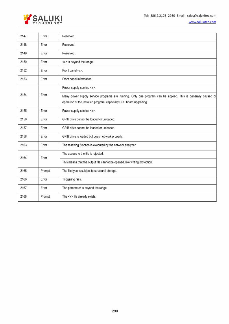
Tel: 886.2.2175 2930 Email: [email protected]
www.salukitec.com
290
2147 Error Reserved.
2148 Error Reserved.
2149 Error Reserved.
2150 Error <x> is beyond the range.
2152 Error Front panel <x>.
2153 Error Front panel information.
2154 Error
Power supply service <x>.
Many power supply service programs are running. Only one program can be applied. This is generally caused byoperation of the installed program, especially CPU board upgrading.
2155 Error Power supply service <x>.
2156 Error GPIB drive cannot be loaded or unloaded.
2157 Error GPIB drive cannot be loaded or unloaded.
2158 Error GPIB drive is loaded but does not work properly.
2163 Error The resetting function is executed by the network analyzer.
2164 ErrorThe access to the file is rejected.
This means that the output file cannot be opened, like writing protection.
2165 Prompt The file type is subject to structural storage.
2166 Error Triggering fails.
2167 Error The parameter is beyond the range.
2168 Prompt The <x> file already exists.

Tel: 886.2.2175 2930 Email: [email protected]
www.salukitec.com
291
11. Technical Indicators and Measurement MethodsThis chapter describes the technical indicators and measurement methods of S3602 series vector network analyzers.
Technical indicators
Measurement methods·
11.1. Technical Indicators
This section lists the details of performance indicators and technical parameters of S3602 series vector network analyzers. Byreading this section, the user will have an accurate understanding on main performance indicators of the product. Normal workingconditions of the instrument include the ambient temperature of 0°C to +40°C and 1 standard atmospheric pressure.
Main technical parameters of S3602 series vector network analyzers are given below. The temperature of test environment shouldbe 23±3°C, and the ambient temperature change must not exceed ±1°C after calibration. The pressure should be the atmosphericpressure.
Different models and options:
S3602A/B/C/D/E are respectively used to test the frequency of 13.5GHz/26.5GHz/43.5GHz/50GHz/67GHz.
S3602A/B/C/D/E of standard configuration can be used to test the indicators of Port 1 and 2. The four-port type S3602A/B/C/D/Ecan be used to test the indicators of Port 1, 2, 3 and 4.
11.1.1. Frequency RangeFrequency range:
S3602A: 10MHz to 13.5GHz
S3602B: 10MHz to 26.5GHz
S3602C: 10MHz to 43.5GHz S3602D: 10MHz to 50GHz
S3602E: 10MHz to 67GHz
11.1.2. Frequency Accuracy
Frequency accuracy: ±1×10⁻⁷ (23±3)
11.1.3. Frequency ResolutionFrequency resolution: 1Hz
11.1.4. Port Output Harmonic SuppressionTable 11.1 Indicators of S3602A/B Port Output Harmonic Suppression
(Power setting: -5dBm, 2/3 harmonics)
Frequency range 10MHz≤f≤4GHz 4GHz<f≤13.5GHz 13.5GHz<f≤26.5GHz
Output harmonic suppression of Port 1 and 3 -51dBc -60dBc -60dBc
Output harmonic suppression of Port 2 and 4 -13dBc -21dBc -21dBc
Table 11.1 Indicators of S3602C/D Port Output Harmonic Suppression (continued)
(Power setting: -5dBm, 2/3 harmonics)

Tel: 886.2.2175 2930 Email: [email protected]
www.salukitec.com
292
Frequency range 10MHz≤f≤4GHz 4GHz<f≤13.5GHz 13.5GHz<f≤67GHz
Output harmonic suppression of Port 1 and 3 -51dBc -60dBc -60dBc
Output harmonic suppression of Port 2 and 4 -13dBc -21dBc -60dBc
11.1.5. Maximum Output Power of PortTable 11.2-1 Maximum Output Power Indicator of S3602A/B Test Port
Description
Standard, Option 400 Option 201,401,402
Port 1,3Port 2,4
Port 1,3Port 2,4
Filtered Mode Hi Power Mode Filtered Mode Hi Power Mode
10MHz to 50MHz 0dBm +9dBm +13dBm -1dBm +8dBm +12dBm
50MHz to 4GHz 0dBm +6dBm +13dBm -1dBm +5dBm +12dBm
4GHz to 7GHz +12dBm +10dBm +10dBm +9dBm
7GHz to 13.5GHz +8dBm +9dBm +6dBm +8dBm
13.5GHz to 20GHz +6dBm +9dBm +4dBm +5dBm
20GHz to 26.5GHz +4dBm +2dBm +2dBm +0dBm
Table 11.2-2 Maximum Output Power Indicator of S3602C/D Test Port
Description
Standard, Option 400 Option 201,401,402
Port 1,3Port 2,4
Port 1,3Port 2,4
Filtered Mode Hi Power Mode Filtered Mode Hi Power Mode
10MHz to 50MHz -1dBm +8dBm +11dBm -2dBm +8dBm +10dBm
50MHz to 4GHz 0dBm +5dBm +9dBm -1dBm +5dBm +8dBm
4GHz to 13.5GHz +5dBm +6dBm +3dBm +4dBm
13.5GHz to 40GHz +7dBm +7dBm +5dBm +5dBm
40GHz to 47GHz +5dBm +5dBm +2dBm +2dBm
47GHz to 50GHz -5dBm -7dBm -10dBm -10dBm
Table 11.2-3 Maximum Output Power Indicator of S3602E Test Port
Description
Standard, Option 400 Option 201,401,402
Port 1,3Port 2,4
Port 1,3Port 2,4
Filtered Mode Hi Power Mode Filtered Mode Hi Power Mode
10MHz to 50MHz -1dBm +8dBm +8dBm -2dBm +7dBm +7dBm
50MHz to 4GHz 0dBm +5dBm +5dBm -1dBm +4dBm +4dBm
4GHz to 13.5GHz +1dBm +1dBm -2dBm -2dBm
13.5GHz to 26.5GHz +5dBm +5dBm +3dBm +3dBm

Tel: 886.2.2175 2930 Email: [email protected]
www.salukitec.com
293
Description
Standard, Option 400 Option 201,401,402
Port 1,3Port 2,4
Port 1,3Port 2,4
Filtered Mode Hi Power Mode Filtered Mode Hi Power Mode
26.5GHz to 40GHz +3dBm +3dBm 0dBm 0dBm
40GHz to 67GHz +5dBm +5dBm 0dBm 0dBm
11.1.6. Accuracy of Port Output PowerAccuracy of port output power (power setting: -5dBm):
±2dB 10MHz≤f≤13.5GHz
±3dB 13.5GHz<f≤26.5GHz
±3dB 26.5GHz<f≤40GHz
±4dB 40GHz<f≤43.5GHz
±4dB 43.5GHz<f≤67GHz
11.1.7. Output Power Sweep RangeTable 11.3 Indicators of S3602A/B Power sweep Range
Frequency Range Power Sweep RangeS3602A/B S3602C/D S3602E
10MHz≤f≤50MHz 33dB 32dB 32dB
50MHz<f≤4GHz 30dB 29dB 29dB
4GHz<f≤7GHz 34dB28dB
28dB7GHz<f≤13.5GHz 31dB
13.5GHz<f≤20GHz 29dB
30dB20GHz<f≤26.5GHz 25dB
26.5GHz≤f≤35GHz
NA
29dB35GHz<f≤40GHz 26dB
40GHz<f≤47GHz 27dB25dB
47GHz<f≤67GHz NA
11.1.8. Linearity of Port Output Power
Linearity of port output power (23±3): ±2.0dB
11.1.9. 1dB Compression Level of Port1dB compression level of S3602A/B port:
+10dBm 10MHz≤f≤13.5GHz
+10dBm 13.5GHz<f≤16GHz
+2dBm 16GHz<f≤26.5GHz
1dB compression level of S3602C/D port:
+8dBm 10MHz≤f≤40GHz
+5dBm 40GHz<f≤43.5GHz

Tel: 886.2.2175 2930 Email: [email protected]
www.salukitec.com
294
+5dBm 43.5GHz<f≤50GHz
11.1.10. System Trace NoiseTable 11.5 S3602 System Trace Noise
(Power setting: -5dBm; IF bandwidth: 1kHz)
Frequency range S3602 A/B S3602 C/D S3602 EAmplitude Trace Phase Trace Amplitude Trace Phase Trace Amplitude Trace Phase Trace
10MHz≤f≤50MHz ≤0.050 dB ≤0.200° ≤0.050 dB ≤0.900° ≤0.050 dB ≤0.900°50MHz≤f≤500MHz ≤0.007 dB ≤0.051° ≤0.020 dB ≤0.700° ≤0.020 dB ≤0.700°
500MHz<f≤13.5GHz ≤0.002 dB ≤0.042° ≤0.005 dB ≤0.040° ≤0.005 dB ≤0.040°
13.5GHz<f≤20GHz ≤0.003 dB ≤0.054° ≤0.004 dB ≤0.050° ≤0.004 dB ≤0.050°
20GHz<f≤26.5GHz ≤0.005 dB ≤0.054° ≤0.004 dB ≤0.050° ≤0.004 dB ≤0.050°
26.5GHz<f≤50GHz NA NA ≤0.008 dB ≤0.060° ≤0.020 dB ≤0.100°
50GHz<f≤67GHz NA NA NA NA ≤0.020 dB ≤0.100°
11.1.11. Dynamic Range of SystemTable 11.6 Dynamic Range Indicators of System
(Power setting: maximum port output power; IF bandwidth: 1Hz; 23±3)
Frequency range Dynamic Range of SystemS3602A/B S3602C/D S3602E
10MHz≤f≤1GHz 90dB 74dB 74dB
1GHz<f≤4GHz 120dB 119dB 90dB
4GHz<f≤10GHz 127dB 119dB 107dB
10GHz<f≤13.5GHz 120dB 119dB 110dB
13.5GHz<f≤20GHz 120dB 115dB 110dB
20GHz<f≤24GHz 115dB 115dB 110dB
24GHz<f≤26.5GHz 110dB 115dB 110dB
26.5GHz≤f≤35GHz NA 110dB 100dB35GHz<f≤47GHz NA 105dB 90dB
47GHz<f≤50GHz NA 92dB 90dB
50GHz<f≤67GHz NA NA NA
11.1.12. Transmission Tracking, Reflection Tracking, Effective Source Matching and EffectiveDirection
Table 11.7 Transmission Tracking, Reflection Tracking, Effective Source Matching, Effective Direction and Effective Load Matching of S3602A/B
(Power setting: -5dBm; IF bandwidth: 10Hz, 23±3)
Frequency range 10MHz≤f≤2GHz 2GHz<f≤13.5GHz 13.5GHz<f≤26.5GHz
Transmission tracking ±0.10dB ±0.11dB ±0.12dB
Reflection tracking ±0.04dB ±0.04dB ±0.05dB
Effective direction; ≥48dB ≥44dB ≥44dB
Effective source matching; ≥40dB ≥30dB ≥30dB

Tel: 886.2.2175 2930 Email: [email protected]
www.salukitec.com
295
Effective load matching; ≥48dB ≥44dB ≥44dB
Table 11.7 Transmission Tracking, Reflection Tracking, Effective Source Matching, Effective Direction and Effective Load Matching of S3602C/D
(Power setting: -5dBm; IF bandwidth: 10Hz, 23±3)
Frequency range 10MHz≤f≤2GHz 2GHz<f≤13.5GHz 13.5GHz<f≤40GHz 40GHz<f≤50GHz
Transmission tracking ±0.10dB ±0.11dB ±0.16dB ±0.20dB
Reflection tracking ±0.04dB ±0.04dB ±0.03dB ±0.04dB
Effective direction; ≥42dB ≥42dB ≥38dB ≥36dB
Effective sourcematching;
≥36dB ≥31dB ≥28dB ≥27dB
Effective loadmatching;
≥42dB ≥42dB ≥37dB ≥35dB
Table 11.7 Transmission Tracking, Reflection Tracking, Effective Source Matching, Effective Direction and Effective Load Matching of S3602C/D
(Power setting: -5dBm; IF bandwidth: 10Hz, 23±3)
Frequency range 10MHz≤f≤2GHz 2GHz<f≤13.5GHz 13.5GHz<f≤40GHz 40GHz<f≤67GHz
Transmission tracking ±0.10dB ±0.11dB ±0.16dB ±0.20dB
Reflection tracking ±0.05dB ±0.06dB ±0.08dB ±0.10dB
Effective direction; ≥35dB ≥41dB ≥34dB ≥32dB
Effective sourcematching;
≥35dB ≥31dB ≥28dB ≥25dB
Effective loadmatching;
≥35dB ≥41dB ≥33dB ≥30dB
11.1.13. Falling Time of Pulse ModulationFalling time of pulse modulation: ≤30ns 500MHz≤f≤50GHz
11.1.14. Pulse Modulation Switching RatioTable 11.8 Indicators of Pulse Modulation Switching Ratio
Frequency range 10MHz≤f≤4GHz 4<f≤50GHz
Switch ratio of pulse modulation ≥64dB ≥80dB
11.1.15. Port Damage LevelPort damage level: 26dBm or 30VDC.
Limit level of port damage: +26dBm or 30VDC. If the input is beyond the above range, the instrument may be burnt.
11.1.16. Operation Temperature and Storage TemperatureTable 11.9 Range of Working Temperature and Storage Temperature

Tel: 886.2.2175 2930 Email: [email protected]
www.salukitec.com
296
Operating temperature range 0°C-40
Storage temperature range -30°C - 70°C
11.1.17. Number of Measurement PointsThe number of measurement points in each frequency sweep of S3602 series vector network analyzers can be set between 1 and32001.
11.1.18. Measurement Display Format
S3602 series vector network analyzers have the following measurement display options: logarithmic amplitude, linear amplitude,standing wave ratio, phase, group delay, real part, imaginary part, Smith chart, and polar coordinates.
11.1.19. Display Window and Channel
S3602 series vector network analyzers are equipped with a 12.1-inch color LCD display, with the resolution of 1280×800. At most 16windows and 64 channels can be set. Each window supports 8 optional channels at most. All channels can be used for display atthe same time. Each channel can be used to separately display basic S- parameters such as S11 and S21.
11.1.20. Averaging FactorAveraging factor range of S3602 series vector network analyzers: 1-1024.
11.1.21. Marker FunctionS3602 series vector network analyzers are configured with 9 independent marker to read and display the value of the measurementcurve. Specific functions are as follows.
a) marker search function: used for automatic search on the measurement curve, such as the maximum value, minimum value,right peak value, left peak value, etc.
b) function: used to read the difference between the current marker and reference marker.
c) Marker function: used to set the current starting value, ending value, center value, span, reference value and delay time as theactive marker value.
d) Bandwidth search function: used for automatic search to set the bandwidth (it can be set by the user, and the default value is3dB) and calculate the Q value.
11.1.22. Sweep TypeS3602 series vector network analyzers are configured with 5 scanning types:
a) Linear frequency: default sweep type of the instrument. The frequency linearity continuously covers the whole frequencyrange.
b) Logarithmic frequency: the source frequency increases in the logarithmic step manner, and the frequency ratio of two adjacentfrequency points is identical.
c) Power sweep: used in the CW mode.
d) CW: set the single sweep frequency of the analyzer, continuously and accurately sample measurement data according to theinterval determined with the sweep time and measurement point number, and display measurement data changes over time.
e) Segment sweep: set the enabling of sweep involving multiple segments. The power level, IF bandwidth and sweep time ofeach segment can be defined separately.
11.1.23. Intermediate Frequency Bandwidth
Intermediate frequency bandwidth: min. 1Hz and max. 5MHz; stepping modes: 40 in total.
11.1.24. Setting of Reference Level Amplitude

Tel: 886.2.2175 2930 Email: [email protected]
www.salukitec.com
297
Setting range: ±500dB
Setting resolution: 0.001dB
11.1.25. Setting of Reference PhaseSetting range: ±500°
Setting resolution: 0.01°
11.1.26. Storage FunctionThe following files can be saved: state calibration files (*.cst), state files (*.sta), calibration files (*.cal), data files (*.dat, *.cti, *.s1p,*.s2p, *.s3p and *.s4p), table files (*.prn) and graphical files (*.bmp and *.jpg).
11.1.27. Port Type
S3602A/B: 3.5mm standard connector (male)
S3602C/D: 2.4mm standard connector (male)
S3602E: 1.8mm standard connector (male)
11.1.28. 11.1.28 Interface Types
Peripheral interfaces include: GPIB interface, USB interface, monitor interface and LAN interface.

Tel: 886.2.2175 2930 Email: [email protected]
www.salukitec.com
298
11.2. Measurement Methods
Following test procedures is made for S3602B. For other models, the procedures are similar.
Test of frequency accuracy
Test of frequency resolution
Test of port output harmonic suppression
Test of non-harmonic suppression of port output
Test of maximum output power of port
Test of port output power accuracy
Test of sweep range of port output power
Linearity of port output power
Test of 1dB compression level of port
Test of system trace noise
Test of dynamic range of system
Test of transmission tracking, reflection tracking, effective source matching, effective direction and effective load matching
Test of rising/falling time of pulse modulation
Test of pulse modulation switching ratio
11.2.1. Test of Frequency Accuracy
11.2.1.1. Items of Frequency Accuracy Test
Test the frequency accuracy indicators of frequency sweep signals output by S3602 series vector network analyzers.
11.2.1.2. Instrument and Accessories for Test of Frequency Range and Accuracy
1) Frequency meter HP5361B
2) RF cable 1.
Fig.11.1 Block Diagram of Frequency Accuracy Test
11.2.1.3. Steps of Frequency Accuracy Test1) As shown in Fig. 11.1, connect the system and preheat is for 60min at least.
2) Press [Reset] to set the initial state of S3602 series vector network analyzers.
3) Press [Stimulus] > [Sweep] > [CW] > [Frequency], and enter 10GHz. Press [Stimulus] > [Trigger] > [Hold]. The reading of thefrequency meter will be the frequency of the stimulus signal of the analyzer.
11.2.2. Test of Frequency Resolution
Tel: 886.2.2175 2930 Email: [email protected]
www.salukitec.com
299
11.2.2.1. Items of Frequency Resolution TestTest the frequency resolution indicators of frequency scanning signals output by S3602 series vector network analyzers.
11.2.2.2. Instrument and Accessories for Test of Frequency Resolution
1) spectrum analyzer 1
2) BNC cable 1.3) RF cable 1.
11.2.2.3. Steps of Frequency Resolution Test1) As shown in Fig. 11.2, connect the system and preheat is for 60min at least.
2) Press [Reset] to set the initial state of S3602 series vector network analyzers.
3) Press [Sweep] > [Sweep type] > [CW] > [Frequency], and enter 10GHz. Press [Stimulus] > [Trigger] > [Hold]. Record themeasurement result of the spectrum analyzer.
4) Change the center frequency by 1Hz. If the reading of the spectrum analyzer also changes by 1Hz, the frequency resolutionconforms to the technical indicator requirements.
Fig. 11.2 Block Diagram of Frequency Resolution Test
11.2.3. Test of Port Output Harmonic Suppression
11.2.3.1. Items of Test of Port Output Harmonic SuppressionTest the harmonic suppression indicators of frequency sweep signals output by the port of S3602 series vector network analyzers.
11.2.3.2. Instrument and Accessories for Test of Port Output Harmonic Suppression
1) Spectrum analyzer R&SFSUP50
2) RF cable 1.
11.2.3.3. Steps of Test of Port Output Harmonic Suppression1) As shown in Fig. 11.3, connect the system and preheat is for 60min at least.
2) Press [Reset] to set the initial state of S3602 series vector network analyzers. Click [Channel] > [Hardware configuration] >[Path configuration]. Select the filtering mode for the low-frequency segment of Port 1 and 3. Press [Power] > [-5] and theENTER key.
3) Press [Sweep] > [Sweep time] > [10] and the ENTER key.
4) Press [Sweep] > [Sweep type] > [CW] > [Frequency], and enter 10MHz. Set the corresponding test frequency of the spectrumanalyzer and record the reading of the spectrum analyzer. Set the second harmonic frequency of the spectrum analyzer as20MHz and record the reading of the spectrum analyzer. The difference of two readings is the port harmonic suppressionindicator.

Tel: 886.2.2175 2930 Email: [email protected]
www.salukitec.com
300
Fig. 11.3 Block Diagram of Test of Harmonic/Non-harmonic Suppression Test
11.2.4. Test of Non-harmonic Suppression of Port Output
11.2.4.1. Items of Test of Non-harmonic Suppression of Port Output
Test the non-harmonic suppression indicators of frequency sweep signals output by the port of S3602 series vector networkanalyzers.
11.2.4.2. Instrument and Accessories for Test of Non-harmonic Suppression of Port Output
1) spectrum analyzer AV4038 or R&SFSUP50
2) RF cable 1.
11.2.4.3. eps of Test of Non-harmonic Suppression of Port Output
1) As shown in Fig. 11.3, connect the system and preheat is for 60min at least.
2) Press [Reset] to set the initial state of the S3602 series vector network analyzer. Click [Channel] > [Hardware configuration] >[Path configuration]. Select the filtering mode for the low-frequency segment of Port 1 and 3. Press [Power] > [-5] and theENTER key.
3) Press [Sweep] > [Sweep time] > [10] and the ENTER key.
4) Press [Scanning] > [Sweep type] > [CW] > [Frequency], and enter 10MHz. Set the corresponding test frequency of thespectrum analyzer and record the reading of the spectrum analyzer. Search the maximum power of the non-harmonic signalwith the frequency offset of 30kHz to 5MHz. The difference of two values is the non- harmonic suppression indicator.
5) Respectively change the test frequency of the vector network analyzer and spectrum analyzer. Repeat Step (4) and measurethe non-harmonic suppression indicators of other frequency points.
11.2.5. Test of Maximum Output Power of Port
11.2.5.1. Items of Test of Maximum Output Power of PortTest the maximum output power indicators of the port of S3602 series vector network analyzers.
11.2.5.2. Required Instrument and Accessories
1) Power meter ML2437A
2) Power probe MA2475A
11.2.5.3. Steps of Test of Maximum Output Power of Port
1) As shown in Fig. 11.4, connect the system and preheat is for 60min at least.
2) Press [Reset] > [Power] > [+20] and the ENTER key.
3) Press [Sweep] > [Sweep time] > [20] and the ENTER key.
4) Press [Frequency] > [Starting frequency] and enter the starting frequency 10MHz. Press [Ending frequency] and enter the

Tel: 886.2.2175 2930 Email: [email protected]
www.salukitec.com
301
ending frequency 50MHz.
5) As shown in Fig. 11.4, calibrate/clear the power meter, connect the power probe to Port 1 and record the minimum reading.
6) Successively change the sweep frequency of the S3602 series vector network analyzer. In the high power mode or filter moderequired in the test, click [Channel] > [Hardware configuration] > [Path configuration]. Select the high power mode or filteringmode for the low-frequency segment of Source 1. The test result is the maximum output power of Port 1.
7) Connect the power probe to Port 2/3/4. Click [Measurement] > [S22]/[S33]/[S44]. Repeat Step (4) to (6) and measure themaximum output power of Port 2/3/4.
Fig. 11.4 Block Diagram of Port Output Power Test
11.2.6. Test of Port Output Power Accuracy
11.2.6.1. Items of Test of Port Output Power Accuracy
Test the port output power accuracy indicators of V3602 series vector network analyzers.
11.2.6.2. Instrument and Accessories for Test of Port Output Power Accuracy
1) Power meter ML2437A
2) Power probe MA2475A
11.2.6.3. Steps of Test of Port Output Power Accuracy
1) As shown in Fig. 11.4, connect the system and preheat is for 60min at least. Press [Reset] > [Sweep] > [Sweep time] > [10]and the ENTER key. Press [Power] > [-5] and the ENTER key.
2) Press [Sweep] > [Scanning type] > [CW] > [Frequency] and enter 10MHz.
3) As shown in Fig. 11.4, connect the power probe, and record the reading.
4) Change the frequency point successively, and record the measurement result of the output power accuracy of Port 1.
5) Connect the power probe to Port 2/3/4. Click [Measurement] > [S22]/[S33]/[S44]. Measure the output power accuracy of Port2/3/4.
11.2.7. Test of sweep Range of Port Output Power
11.2.7.1. Items of Test of sweep Range of Port Output Power
Test the sweep range indicators of the port output power of S3602 series vector network analyzers.
11.2.7.2. Instrument and Accessories for Test of sweep Range of Port Output Power
1) Power meter AV2434 or ML2437A
2) Power probe AV71711 or MA2475A3) RF cable 1.
11.2.7.3. Steps of Test of sweep Range of Port Output Power

Tel: 886.2.2175 2930 Email: [email protected]
www.salukitec.com
302
1) As shown in Fig. 11.4, connect the system and preheat is for 60min at least. Press [Reset] > [Sweep] > [Sweep time] > [20]and the ENTER key. Click [Channel] > [Hardware configuration] > [Path configuration]. Select the high power mode for thelow-frequency segment of Source 1 and 3.
2) Press [Sweep] > [Sweep type] > [Frequency sweep]. Set the starting frequency as -30dBm and ending frequency as +20dBm.
3) Press [Frequency] and enter 10MHz.
4) As shown in Fig. 11.4, connect the power probe. Observe the reading of the power meter. The difference between themaximum and minimum value is the power sweep range. Change frequency points and measure the corresponding powersweep ranges.
5) Connect the power probe to Port 2/3/4. Click [Measurement] > [S22]/[S33]/[S44]. Measure the output power sweep ranges ofother ports.
11.2.8. Linearity of Port Output Power
11.2.8.1. Items of Test of Port Output Power LinearityTest the port output power linearity indicators of S3602 series vector network analyzers.
11.2.8.2. Instrument and Accessories for Test of Port Output Power Linearity1) Soft test cable Agilent 85131F (AV3602A/B) or FE0BN0BM025.0 (AV3602C/D)
11.2.8.3. eps of Test of Port Output Power Linearity1) As shown in Fig. 11.5, connect the system and preheat is for 60min at least.
2) Click [Reset] > [Response] > [Measurement] > [Measurement...] and [Receiver]. Select [B] and [Port 1] under [Source] portand click [OK].
Fig. 11.5 Output Power Linearity of Test Port
3) Press [Channel] > [More] > [Hardware setting] > [Graphical configuration]. Select [Low-band high-power mode] and click [OK].
4) Press [Power] > [-10] > [OK].
5) Press [Analysis] > [Memory] > [Normalization].
6) Press [Power] > [-25] and the ENTER key to change the power into -25dBm. After sweep once, press [Analysis] > [tracestatistics] > [trace statistics ON/OFF]. Read the maximum and minimum value. Calculate the differences of the (absolutionmaximum and minimum value+10) minus the set power. The larger absolute value of two results is the power linearity.
7) Successively change the power and record the linearity value corresponding to each power value within 10MHz- 50GHz.
11.2.9. dB Compression Level Test of Port
11.2.9.1. Items of 1dB Compression Level Test of Port
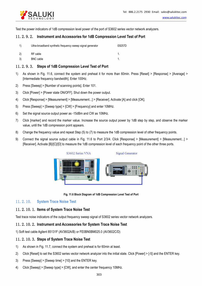
Tel: 886.2.2175 2930 Email: [email protected]
www.salukitec.com
303
Test the power indicators of 1dB compression level power of the port of S3602 series vector network analyzers.
11.2.9.2. Instrument and Accessories for 1dB Compression Level Test of Port
1) Ultra-broadband synthetic frequency sweep signal generator E8257D
2) RF cable 1.3) BNC cable 1.
11.2.9.3. Steps of 1dB Compression Level Test of Port
1) As shown in Fig. 11.6, connect the system and preheat it for more than 60min. Press [Reset] > [Response] > [Average] >[Intermediate frequency bandwidth]. Enter 100Hz.
2) Press [Sweep] > [Number of scanning points]. Enter 101.
3) Click [Power] > [Power state ON/OFF]. Shut down the power output.
4) Click [Response] > [Measurement] > [Measurement...] > [Receiver]. Activate [A] and click [OK].
5) Press [Sweep] > [Sweep type] > [CW] > [Frequency] and enter 10MHz.
6) Set the signal source output power as -15dBm and CW as 10MHz.
7) Click [marker] and record the marker value. Increase the source output power by 1dB step by step, and observe the markervalue, until the 1dB compression point appears.
8) Change the frequency value and repeat Step (5) to (7) to measure the 1dB compression level of other frequency points.
9) Connect the signal source output cable in Fig. 11.6 to Port 2/3/4. Click [Response] > [Measurement] > [Measurement...] >[Receiver]. Activate [B]/[C]/[D] to measure the 1dB compression level of each frequency point of the other three ports.
Fig. 11.6 Block Diagram of 1dB Compression Level Test of Port
11.2.10. System Trace Noise Test
11.2.10.1. Items of System Trace Noise Test
Test trace noise indicators of the output frequency sweep signal of S3602 series vector network analyzers.
11.2.10.2. Instrument and Accessories for System Trace Noise Test
1) Soft test cable Agilent 85131F (AV3602A/B) or FE0BN0BM025.0 (AV3602C/D)
11.2.10.3. Steps of System Trace Noise Test
1) As shown in Fig. 11.7, connect the system and preheat is for 60min at least.
2) Click [Reset] to set the S3602 series vector network analyzer into the initial state. Click [Power] > [-5] and the ENTER key.
3) Press [Sweep] > [Sweep time] > [10] and the ENTER key.
4) Click [Sweep] > [Sweep type] > [CW], and enter the center frequency 10MHz.
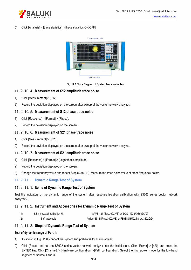
Tel: 886.2.2175 2930 Email: [email protected]
www.salukitec.com
304
5) Click [Analysis] > [trace statistics] > [trace statistics ON/OFF].
Fig. 11.7 Block Diagram of System Trace Noise Test
11.2.10.4. Measurement of S12 amplitude trace noise
1) Click [Measurement] > [S12].
2) Record the deviation displayed on the screen after sweep of the vector network analyzer.
11.2.10.5. Measurement of S12 phase trace noise1) Click [Response] > [Format] > [Phase].
2) Record the deviation displayed on the screen.
11.2.10.6. Measurement of S21 phase trace noise1) Click [Measurement] > [S21].
2) Record the deviation displayed on the screen after sweep of the vector network analyzer.
11.2.10.7. Measurement of S21 amplitude trace noise
1) Click [Response] > [Format] > [Logarithmic amplitude].
2) Record the deviation displayed on the screen.
3) Change the frequency value and repeat Step (4) to (13). Measure the trace noise value of other frequency points.
11.2.11. Dynamic Range Test of System
11.2.11.1. Items of Dynamic Range Test of System
Test the indicators of the dynamic range of the system after response isolation calibration with S3602 series vector networkanalyzers.
11.2.11.2. Instrument and Accessories for Dynamic Range Test of System
1) 3.5mm coaxial calibration kit SAV31121 (SAV3602A/B) or SAV31123 (AV3602C/D)2) Soft test cable Agilent 85131F (AV3602A/B) or FE0BN0BM025.0 (AV3602C/D)
11.2.11.3. Steps of Dynamic Range Test of System
Test of dynamic range of Port 1:
1) As shown in Fig. 11.8, connect the system and preheat is for 60min at least.
2) Click [Reset] and set the S3602 series vector network analyzer into the initial state. Click [Power] > [+20] and press theENTER key. Click [Channel] > [Hardware configuration] >[Path configuration]. Select the high power mode for the low-bandsegment of Source 1 and 3.

Tel: 886.2.2175 2930 Email: [email protected]
www.salukitec.com
305
3) Click [Measurement] > [S12].
4) Click [Scale] > [Reference value] and enter -100.
5) Click [Sweep] > [Number of sweep points], and enter 101.
6) Click [Response] > [Average] > [Intermediate frequency bandwidth], and enter 1Hz.
7) Click [Calibration] > [Non-guided calibration] and [Through type response and isolation].
8) Click [Selection of calibration kit] > [AV31121] > [Through type] to start through type calibration.
9) After through type calibration, as shown in Fig. 11.9, disconnect the tow cables and connect loads to two calibration cableports.
10) Select [Load]. Select [Enable averaging] in the pop-up dialog box. Set the averaging factor as 8, and continue calibration.
11) After all calibrations, click [OK]. Then click [Response] > [Average] > [Averaging factor] and enter 8 to enable the averagingfunction.
12) After averaging, the maximum value of the displayed curve within each frequency range is the dynamic range of Port 1.
Fig. 11.8 Block Diagram I of Dynamic Range Calibration Test of System
Fig. 11.9 Block Diagram II of Dynamic Range Calibration Test of System
Test of dynamic range of Port 2:
13) Click [Measurement] > [S21].
14) Repeat Step (7) to (12) to test the dynamic range of Port 2.
Test of dynamic range of Port 3:
15) As shown in Fig. 11.10, connect the system.
16) Click [Measurement] > [S34].
17) Click [Calibration] > [Non-guided calibration] and [Through type response and isolation].
18) Click [Selection of calibration kit] > [AV31121] > [Through type] to start through type calibration.
19) After through type calibration, as shown in Fig. 11, disconnect the tow cables and connect loads to two calibration cable ports.
20) Select [Load]. Select [Enable averaging] in the pop-up dialog box. Set the averaging factor as 8, and continue calibration.
21) After all calibrations, click [OK]. Then click [Response] > [Average] > [Averaging factor] and enter 8 to enable the averagingfunction.
22) The maximum value of the displayed curve within each frequency range is the dynamic range of Port 3.

Tel: 886.2.2175 2930 Email: [email protected]
www.salukitec.com
306
Fig. 11.10 Block Diagram I of Dynamic Range Calibration Test of System
Fig. 11.11 Block Diagram II of Dynamic Range Calibration Test of System
Test of dynamic range of Port 4:
23) Click [Measurement] > [S43].
24) Repeat Step (18) to (22) to test the dynamic range of Port 4.
11.2.12. Test of Transmission Tracking, Reflection Tracking, Effective Source Matching, EffectiveDirection, etc.
11.2.12.1. Items of Test of Transmission Tracking, Reflection Tracking, Effective Source Matching,Effective Direction and Effective Load Matching
Test the indicators of transmission tracking, reflection tracking, effective source matching, effective direction and effective loadmatching after the full 2-port calibration with S3602 series vector network analyzers.
11.2.12.2. Instrument and Accessories for Test of Transmission Tracking, Reflection Tracking, EffectiveSource Matching, Effective Direction and Effective Load Matching
1) Coaxial calibration kit AV31121 (AV3602A/B) or AV31123 (AV3602C/D)
2) Soft test cable Agilent85131F (AV3602A/B) or FE0BN0BM025.0 (AV3602C/D)
11.2.12.3. Steps of Test of Transmission Tracking, Reflection Tracking, Effective Source Matching,Effective Direction and Effective Load Matching
1) Turn on the instrument and preheat for 60min at least.
2) Press [Reset] to set the S3602 series vector network analyzer into the initial state.
3) Press [Stimulus] > [Power] > [-5] and press [ENTER] key.
4) Press [Stimulus] > [Sweep] > [Number of points], and enter 51.
5) Press [Response] > [Average] > [IF bandwidth], and enter 10Hz.
6) Press [Calibration]. Select [Unguided calibration] > [Full SOLT 2 Port].
7) Press [Select CalKit] > [AV31123].
8) Respectively connect calibration open standards to port 1 as shown in Figure 1. Select [Open] on the pop out calibrationwindow. Wait for calibration process complete.

Tel: 886.2.2175 2930 Email: [email protected]
www.salukitec.com
307
Fig. 11.12 Block Diagram I of Connection of Full 2-port Calibration
9) Repeat Step 8 to do the short and Load calibration for Port 1.
10) Repeat Step 8, 9 to do the SOL calibration for Port 2.
11) When single port calibration is done, connect the system as shown in Fig 2. Select [Through] to start through type calibration.
12) Wait for the calibration completed and disconnect the test cable.Now the instrument now is ready to be tested.
Fig. 11.13 Block Diagram II of Connection of Full 2-port Calibration
Marker Operations
The measurement will need to use Marker operations.
When press [Marker] key, a soft menu will pop out. Then select [Marker Search], the marker search dialog pops out as shown infigure below. In this dialog, user can select a marker, activate the search function (Max, Min etc.) in a configurable frequency span(Full Span /User Span)
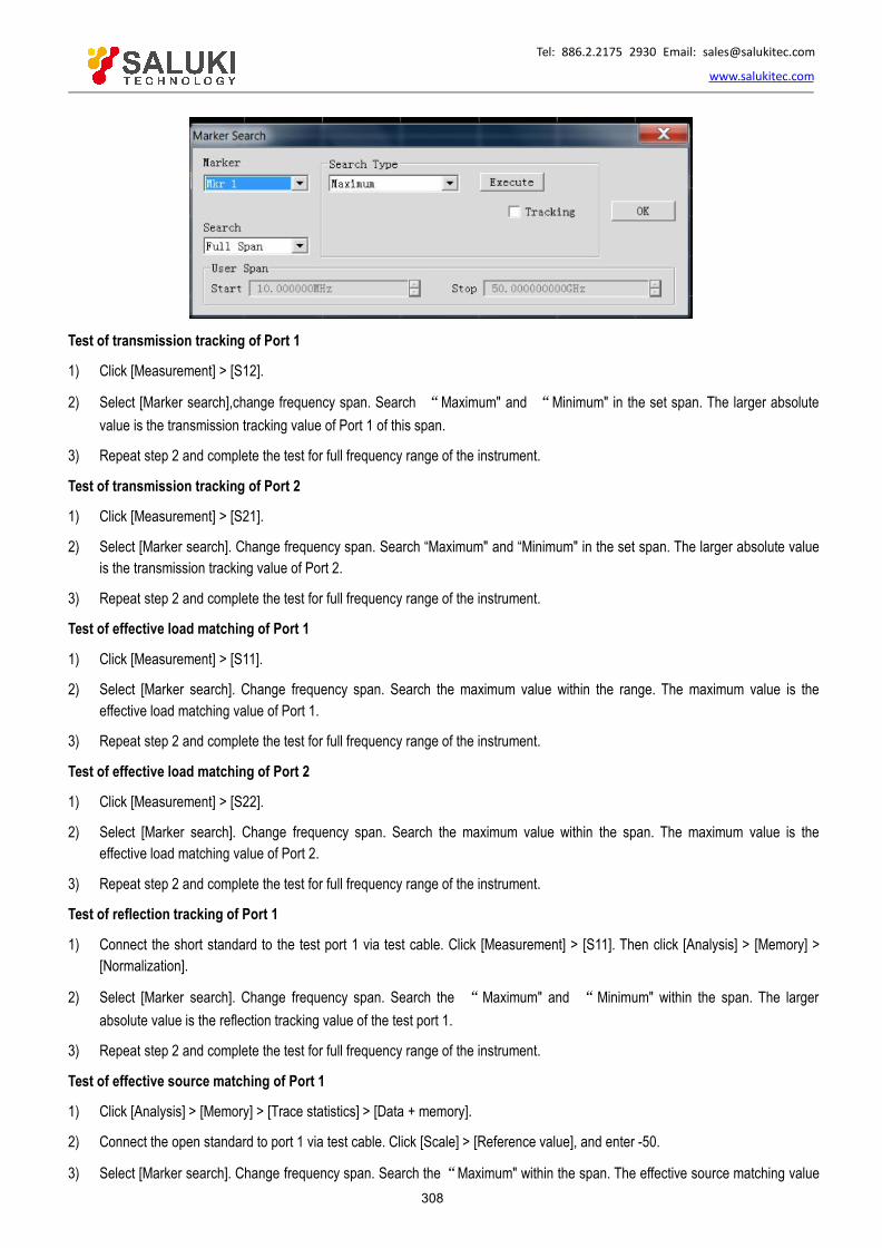
Tel: 886.2.2175 2930 Email: [email protected]
www.salukitec.com
308
Test of transmission tracking of Port 1
1) Click [Measurement] > [S12].
2) Select [Marker search],change frequency span. Search “Maximum" and “Minimum" in the set span. The larger absolutevalue is the transmission tracking value of Port 1 of this span.
3) Repeat step 2 and complete the test for full frequency range of the instrument.
Test of transmission tracking of Port 2
1) Click [Measurement] > [S21].
2) Select [Marker search]. Change frequency span. Search “Maximum" and “Minimum" in the set span. The larger absolute valueis the transmission tracking value of Port 2.
3) Repeat step 2 and complete the test for full frequency range of the instrument.
Test of effective load matching of Port 1
1) Click [Measurement] > [S11].
2) Select [Marker search]. Change frequency span. Search the maximum value within the range. The maximum value is theeffective load matching value of Port 1.
3) Repeat step 2 and complete the test for full frequency range of the instrument.
Test of effective load matching of Port 2
1) Click [Measurement] > [S22].
2) Select [Marker search]. Change frequency span. Search the maximum value within the span. The maximum value is theeffective load matching value of Port 2.
3) Repeat step 2 and complete the test for full frequency range of the instrument.
Test of reflection tracking of Port 1
1) Connect the short standard to the test port 1 via test cable. Click [Measurement] > [S11]. Then click [Analysis] > [Memory] >[Normalization].
2) Select [Marker search]. Change frequency span. Search the “Maximum" and “Minimum" within the span. The largerabsolute value is the reflection tracking value of the test port 1.
3) Repeat step 2 and complete the test for full frequency range of the instrument.
Test of effective source matching of Port 1
1) Click [Analysis] > [Memory] > [Trace statistics] > [Data + memory].
2) Connect the open standard to port 1 via test cable. Click [Scale] > [Reference value], and enter -50.
3) Select [Marker search]. Change frequency span. Search the“Maximum" within the span. The effective source matching value

Tel: 886.2.2175 2930 Email: [email protected]
www.salukitec.com
309
of the test port 1 is the difference of the obtained marker value minus 6
4) Repeat step 3 and complete the test for full frequency range of the instrument.
Test of effective direction of Port 1
1) Connect the load standard to the test port 1 via test cable. Click [Analysis] > [Memory] > [Trace statistics] > [off].
2) Select [Marker search]. Change frequency span. Search the “Maximum" within the span. The maximum value is the effectivedirection value of the test port 1.
3) Repeat step 2 and complete the test for full frequency range of the instrument.
Test of reflection tracking of Port 2
1) Connect the short-circuit device to the test cable end face of the test port 2. Click [Measurement] > [S22]. Then click[Analysis] > [Memory] > [Normalization].
2) Select [Marker search]. Change frequency span. Search the “Maximum" and “Minimum" within the span. The largerabsolute value is the reflection tracking value of the test port 2.
3) Repeat step 2 and complete the test for full frequency range of the instrument.
Test of effective source matching of Port 2
1) Click [Analysis] > [Memory] > [Trace statistics] > [Data + memory].
2) Connect the open standard to port 2 via test cable. Click [Scale] > [Reference value], and enter -50.
3) Select [Marker search]. Change frequency span. Search the“Maximum" within the span. The effective source matching valueof the test port 2 is the difference of the obtained marker value minus 6
4) Repeat step 3 and complete the test for full frequency range of the instrument.
Test of effective direction of Port 2
1) Connect the load to the test port 2. Click [Analysis] > [Memory] > [Trace statistics] > [Close].
2) Select [Marker search]. Change frequency span. Search the “Maximum" within the span. The maximum value is the effectivedirection value of the test port 2.
3) Repeat step 2 and complete the test for full frequency range of the instrument.
Test of transmission tracking of Port 3
4) Click [Measurement] > [S34].
5) Change the starting and ending value of [User domain]. Search the “Maximum" and “Minimum" within the set range. The largerabsolute value is the transmission tracking value of the test port 3.
Test of transmission tracking of Port 4
6) Click [Measurement] > [S43].
7) Change the starting and ending value of [User domain]. Search the “Maximum" and “Minimum" within the set range. The largerabsolute value is the transmission tracking value of the test port 4.
Effective load matching of test port 3
8) Click [Measurement] > [S33].
9) Change the starting and ending value of [User domain]. Search the maximum value within the range. The maximum value isthe effective load matching value of Port 3.
Test of effective load matching of Port 4

Tel: 886.2.2175 2930 Email: [email protected]
www.salukitec.com
310
10) Click [Measurement] > [S44].
11) Change the starting and ending value of [User domain]. Search the maximum value within the range. The maximum value isthe effective load matching value of Port 4.
Test of reflection tracking of Port 3
12) Connect the short-circuit device to the test cable end face of the test port 1. Click [Measurement] > [S33]. Then click[Analysis] > [Memory] > [Normalization].
13) Change the starting and ending value of [User domain]. Search the “Maximum" and “Minimum" within the set range. The largerabsolute value is the reflection tracking value of the test port 3.
Test of effective source matching of Port 3
14) Click [Analysis] > [Memory] > [trace statistic] > [Data + memory].
15) Connect the open-circuit device to the test cable end face of the test port 3. Click [Scale] > [Reference value], and enter -50.
16) Change the starting and ending value of [User domain]. Search the maximum value within the set range. The effective sourcematching value of the test port 3 is the difference of the obtained marker value minus 6.
Test of effective direction of Port 3
17) Connect the load to the test port 3. Click [Analysis] > [Memory] > [trace statistic] > [Close].
18) Change the starting and ending value of [User domain], and search the maximum value within the set range. The maximumvalue is the effective direction value of the test port 3.
Test of reflection tracking of Port 4
19) Connect the short-circuit device to the test cable end face of the test port 4. Click [Measurement] > [S44]. Then click[Analysis] > [Memory] > [Normalization].
20) Change the starting and ending value of [User domain]. Search the “Maximum" and “Minimum" within the set range. The largerabsolute value is the reflection tracking value of the test port 4.
Test of effective source matching of Port 4
21) Click [Analysis] > [Memory] > [trace statistic] > [Data + memory].
22) Connect the open-circuit device to the test cable end face of the test port 4. Click [Scale] > [Reference value], and enter -50.
23) Change the starting and ending value of [User domain]. Search the maximum value within the set range. The effective sourcematching value of the test port 4 is the difference of the obtained marker value minus 6.
Test of effective direction of Port 4
24) Connect the load to the test port 4. Click [Analysis] > [Memory] > [trace statistic] > [Close].
25) Change the starting and ending value of [User domain]. Search the maximum value within the set range. The maximum valueis the effective direction value of the test port 4.
11.2.13. Test of Pulse Modulation Rising/Falling Time
11.2.13.1. Items of Test of Pulse Modulation Rising/Falling TimeTest the pulse modulation rising/falling time indicators of S3602 series vector network analyzers
11.2.13.2. Instrument and Accessories for Test of Pulse Modulation Rising/Falling Time
1) Power meter N1913A
2) Peak power probe N1924A
11.2.13.3. Step of Test of Pulse Modulation Rising/Falling Time

Tel: 886.2.2175 2930 Email: [email protected]
www.salukitec.com
311
1) As shown in Fig. 11.14, connect the system. Click [Reset] to set the S3602 vector network analyzer into the initial state.Preheat the instrument for more than 60min.
Fig. 11.14 Block Diagram of Test of Pulse Modulation Rising/Falling Time Indicators
2) Connect the peak power probe to the calibration port and calibrate the RF power analyzer.
3) Click [Power] > [-10] and the ENTER key.
4) Click [Sweep] > [Sweep type] > [Macro], and enter the center frequency 500MHz. Click [Macro] > [Pulse] > [Narrow bandpulse] > [Source modulation] (interval: 150ns; pulse duration: 60ns; IF gate: 60ns) > [Pulse mode on/off] > [Calculate] > [Apply]to enable the pulse mode.
5) Change the frequency of the S3602 series vector network analyzer and the peak power meter. Repeat Step (4) to (5).
6) Read the measurement result of the peak power meter.
11.2.14. Pulse Modulation Switching Ratio Test
11.2.14.1. Items of Pulse Modulation Switching Ratio Test
Test the switching ratio indicators of the output modulation pulse of S3602 series vector network analyzers.
11.2.14.2. Instrument and Accessories for Pulse Modulation Switching Ratio Test
1) Spectrum analyzer AV4038 or R&S FSUP50
2) BNC cable 1.3) RF cable 1.
11.2.14.3. Steps of Pulse Modulation Switching Ratio Test1) As shown in Fig. 11.15, connect the system and preheat is for 60min at least.
Fig. 11.5 Block Diagram of Pulse Modulation Switching Ratio Test
2) Press [Reset] to set the initial state of S3602 series vector network analyzers.
3) Press [Sweep] > [Sweep type] > [CW] > [Frequency] and enter 10MHz.
4) Set the center frequency of the spectrum analyzer as 10MHz. Adjust the spectrum analyzer and record the signal power P(ON).This power value is equal to the power value corresponding to high pulse modulation input, i.e. “Pulse ON".

Tel: 886.2.2175 2930 Email: [email protected]
www.salukitec.com
312
5) Click [Macro] > [Pulse] > [Configuration] > [Pulse generator/modulator]. Select not to use the internal modulator. Click [Pulsemode] > [Calculate] > [Apply] to enable the pulse mode of the analyzer. As no external pulse signal is connected, theequivalent input signal is low, and the instrument works in the “Pulse OFF" mode. Measure the signal power P(OFF) with thespectrum analyzer and record it.
6) Calculate the difference of the power values measured in the “Pulse ON" and “Pulse OFF" mode. The difference is the actualpulse modulation switching ratio of the tested frequency point.
7) Click [Macro] > [Pulse] > [Pulse mode on/off] > [Apply] to cancel the pulse mode. Modify the frequency point and repeat Step(3) to (6) to obtain the pulse modulation switching ratio of the other frequency points.