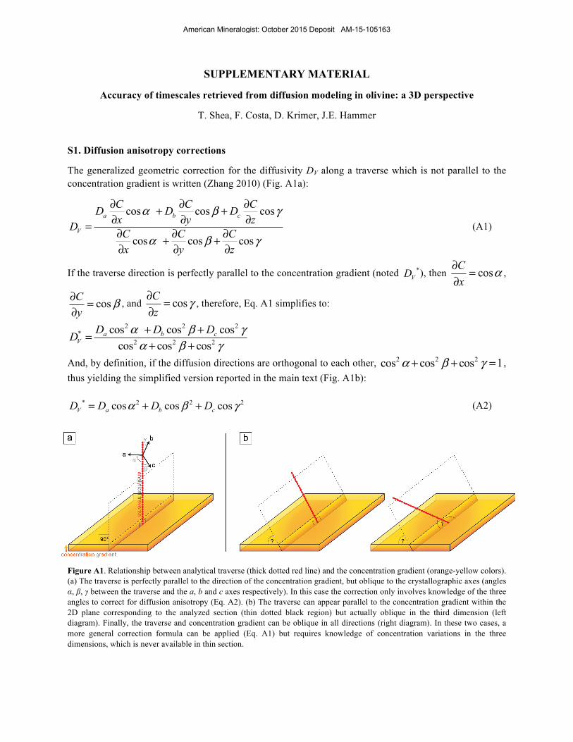
S1. Diffusion anisotropy corrections - SOEST · S1. Diffusion anisotropy corrections ... more...

SUPPLEMENTARY MATERIAL

Accuracy of timescales retrieved from diffusion modeling in olivine: a 3D perspective

T. Shea, F. Costa, D. Krimer, J.E. Hammer

S1. Diffusion anisotropy corrections

The generalized geometric correction for the diffusivity DV along a traverse which is not parallel to the concentration gradient is written (Zhang 2010) (Fig. A1a):

cos cos cos

cos cos cos

a b c

V

C C CD D Dx y zD C C Cx y z

α β γ

α β γ

∂ ∂ ∂+ +∂ ∂ ∂= ∂ ∂ ∂+ +∂ ∂ ∂

(A1)

If the traverse direction is perfectly parallel to the concentration gradient (noted *VD ), then cosC

xα∂ =

∂,

cosCy

β∂ =∂

, and cosCz

γ∂ =∂

, therefore, Eq. A1 simplifies to:

2 2 2*

2 2 2

cos cos coscos cos cos

a b cV

D D DD α β γα β γ+ +=+ +

And, by definition, if the diffusion directions are orthogonal to each other, 2 2 2cos cos cos 1α β γ+ + = , thus yielding the simplified version reported in the main text (Fig. A1b):

* 2 2 2cos cos cosV a b cD D D Dα β γ= + + (A2)

Figure A1. Relationship between analytical traverse (thick dotted red line) and the concentration gradient (orange-yellow colors). (a) The traverse is perfectly parallel to the direction of the concentration gradient, but oblique to the crystallographic axes (angles α, β, γ between the traverse and the a, b and c axes respectively). In this case the correction only involves knowledge of the three angles to correct for diffusion anisotropy (Eq. A2). (b) The traverse can appear parallel to the concentration gradient within the 2D plane corresponding to the analyzed section (thin dotted black region) but actually oblique in the third dimension (left diagram). Finally, the traverse and concentration gradient can be oblique in all directions (right diagram). In these two cases, a more general correction formula can be applied (Eq. A1) but requires knowledge of concentration variations in the three dimensions, which is never available in thin section.

American Mineralogist: October 2015 Deposit AM-15-105163

S2. Numerical implementation of the diffusion models

Finite differences were used to perform diffusion simulations, using distance steps Δx, Δy and Δz, and a numerical grid consists of i×j×k elements (points, pixels or voxels in 1, 2 and 3D). Using a central approximation, the first derivative of Eq. 2 with respect to x is (e.g. Ismail-Zadeh and Tackley 2010):

xCC

xC kjikji

kji Δ−

=∂∂ −+

2,,1,,1

,,

While the second derivative can be expressed as:

2,,1,,,,1

,,2

2 2x

CCCxC kjikjikji

kji Δ+−

=∂∂ −+

The implementation of finite difference derivatives to the time-dependent diffusion formulation (Eq. 2) has the drawback that the numerical scheme requires a stability criterion to be maintained, expressed as (e.g. Press et al. 2007):

RxtD <

ΔΔ2

with R taking the values 0.5 and 0.166 in 1D and 3D calculations respectively. This limits the size of the time and space steps that can be used in the models. To employ a realistic crystal size while maintaining reasonable computation times, a grid of 241×241×241 was used, with a spacing of 2 µm per point/pixel/voxel. This step size yielded olivines ~400 µm in size along the c axis. Typically, 1D diffusion models took a few seconds to a few minutes, while 3D models required up to 4 days to reach completion. A few models were performed using both smaller and larger spatial grids (51, 101, 301 and 401 voxels each side) with the same model parameters (i.e. spatial step sizes were adapted depending on the total grid size so that the crystal was exactly the same in dimension) for comparison. Only for the 51 voxel did concentrations profiles start to display step-like artefacts due to the low resolution, thus confirming that the use of 241 voxels for most models was appropriate to avoid resolution problems.

S3. Quantifying goodness of fit

The mismatch between 1D and 3D timescales were calculated using differences in concentration gradients at each time t, via a simple root-mean square deviation (RMSD) expression:

( )M

CCRMSD M

imeas

ireal∑ −

=

2

where M is the number of points along x, i is the coordinate along x in the profile, Creal is the ‘real’ concentration taken from the 3D model, and Cmeas is the concentration measured in the 1D model which is being evaluated.

S4. Concentration profiles corresponding to center-cut, on axis 1D models

In the main text, Figure 4 shows the best-matching timescales for 1D diffusion models based on ideal profiles along a, b and c. A different perspective can be gained by examining instead the evolution of concentration profiles with time, (i.e., without seeking the best-matching 1D model).


2

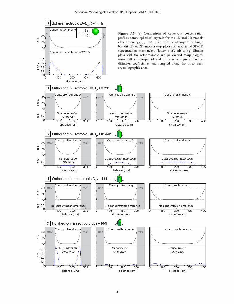
Figure A2. (a) Comparison of center-cut concentration profiles across spherical crystals for the 1D and 3D models after a time t1D=t3D=144 h (i.e. with no attempt at finding a best-fit 1D or 2D model) (top plot) and associated 3D‒1D concentration mismatches (lower plot). (d) to (g) Similar plots with the orthorhombic and polyhedral morphologies, using either isotropic (d and e) or anisotropic (f and g) diffusion coefficients, and sampled along the three main crystallographic axes.


3

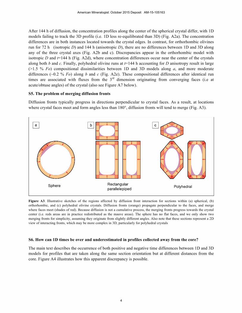
After 144 h of diffusion, the concentration profiles along the center of the spherical crystal differ, with 1D models failing to track the 3D profile (i.e. 1D less re-equilibrated than 3D) (Fig. A2a). The concentration differences are in both instances located towards the crystal edges. In contrast, for orthorhombic olivines run for 72 h (isotropic D) and 144 h (anisotropic D), there are no differences between 1D and 3D along any of the three crystal axes (Fig. A2b and c). Discrepancies appear in the orthorhombic model with isotropic D and t=144 h (Fig. A2d), where concentration differences occur near the center of the crystals along both b and c. Finally, polyhedral olivine runs at t=144 h accounting for D anisotropy result in large (>1.5 % Fo) compositional dissimilarities between 1D and 3D models along a, and more moderate differences (~0.2 % Fo) along b and c (Fig. A2e). These compositional differences after identical run times are associated with fluxes from the 3rd dimension originating from converging faces (i.e at acute/obtuse angles) of the crystal (also see Figure A7 below).

S5. The problem of merging diffusion fronts

Diffusion fronts typically progress in directions perpendicular to crystal faces. As a result, at locations where crystal faces meet and form angles less than 180°, diffusion fronts will tend to merge (Fig. A3).

Figure A3. Illustrative sketches of the regions affected by diffusion front interaction for sections within (a) spherical, (b) orthorhombic, and (c) polyhedral olivine crystals. Diffusion fronts (orange) propagate perpendicular to the faces, and merge where faces meet (shades of red). Because diffusion is not a cumulative process, the merging fronts progress towards the crystal center (i.e. reds areas are in practice redistributed as the mauve areas). The sphere has no flat faces, and we only show two merging fronts for simplicity, assuming they originate from slightly different angles. Also note that these sections represent a 2D view of interacting fronts, which may be more complex in 3D, particularly for polyhedral crystals

S6. How can 1D times be over and underestimated in profiles collected away from the core?

The main text describes the occurrence of both positive and negative time differences between 1D and 3D models for profiles that are taken along the same section orientation but at different distances from the core. Figure A4 illustrates how this apparent discrepancy is possible.


4

Figure A4. Effects of profile distance from the crystal core (measured in % core-rim distance) on 1D times for a spherical olivine. (a) Profiles sampled at increasing distances from the 3D model core, which are then used to compare with 1D models. (b), (c) and (d) display best fit 1D models at increasing distances from the core performed the known initial Fo concentration (i.e., known from the 3D olivine prior to diffusion), while the bottom plots assume that the initial Fo is the minimum apparent value. The shaded regions in each plot represent the total Fo flux required to reach the final profile, as well as associated best-fit times.

S7. How can 1D times be underestimated in center-cut olivine sections preserving core concentrations? A worked example.

In the main text and section S6, we highlighted that time underestimates are fairly common in situations where the initial Fo concentration has been lost, and more so when profiles are collected far away from the core. Nevertheless, Figure 7b and c in the main text also shows that time underestimates occur in profiles that are taken in on-center sections that preserve initial concentrations. This section explains how the simplified anisotropy correction that is used can also yield time underestimates.

Figure A1 above showed that concentration gradients develop perpendicular to crystal faces, and the traverse direction may be oblique to the gradient in the 3rd dimension (despite appearing parallel in 2 dimensions). Therefore, in the numerical comparison between 1D profiles and 3D models, even though the profiles were always selected parallel to the concentration gradient on a 2D slice, the concentration gradient was probably always apparent rather than real compared to the 3rd dimension.

For example, in one of the rectangular olivine simulations, the true angles between the crystallographic axes a, b, c and the transect were α =80.38°, β =32.39°, and γ =59.40°. We assume for this exercise that Da=1, Db=1 and Dc=6. If the traverse is inferred to be parallel to the concentration gradient (Eq. A2) we calculate a diffusivity value * 2.3VD = . If, however, the concentration gradient is at an angle with at least

one of the traverse directions (here for instance the y direction), then Cy

∂∂

will be artificially longer and

overly corrected by Eq. A2 compared to Eq. A1. Leaving cosCx

α∂ =∂

and cosCz

γ∂ =∂

, while

lengthening 1.5cosCy

β∂ =∂

, we obtain 1.95VD = using Eq. A1. Hence, in this case, the simplified


5

anisotropy correction (Eq. A2) tends to overestimate the effective diffusivity, and results in time underestimates.

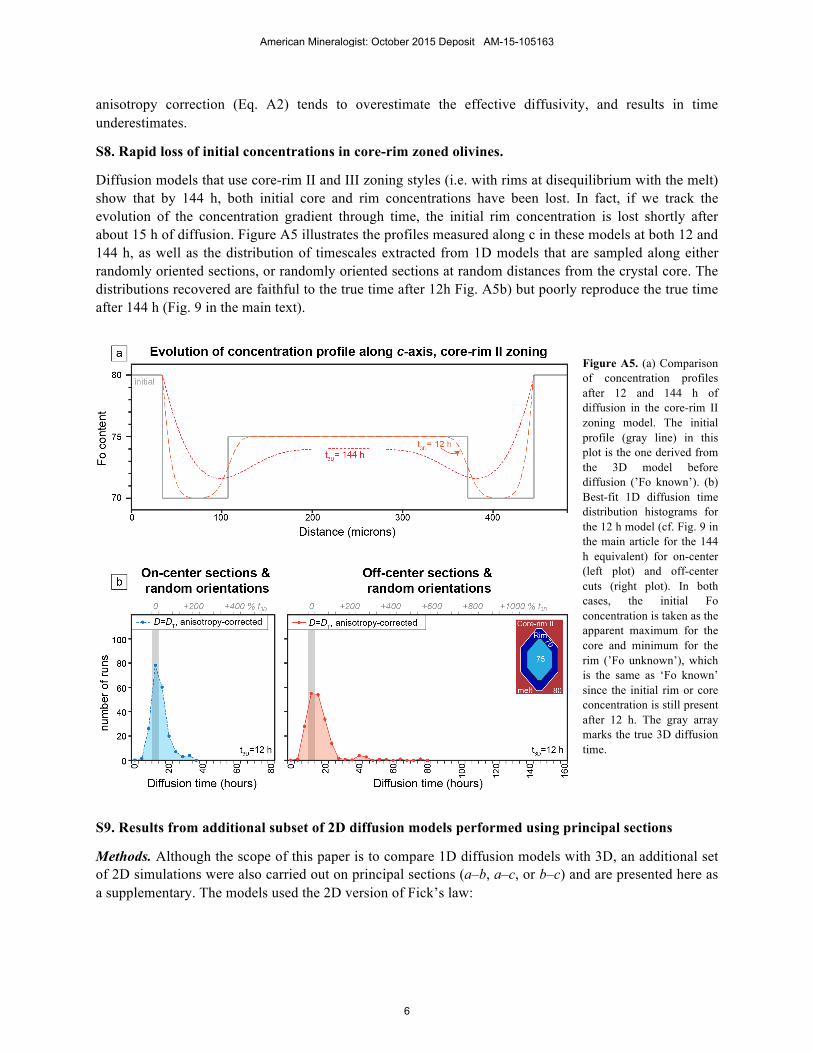
S8. Rapid loss of initial concentrations in core-rim zoned olivines.

Diffusion models that use core-rim II and III zoning styles (i.e. with rims at disequilibrium with the melt) show that by 144 h, both initial core and rim concentrations have been lost. In fact, if we track the evolution of the concentration gradient through time, the initial rim concentration is lost shortly after about 15 h of diffusion. Figure A5 illustrates the profiles measured along c in these models at both 12 and 144 h, as well as the distribution of timescales extracted from 1D models that are sampled along either randomly oriented sections, or randomly oriented sections at random distances from the crystal core. The distributions recovered are faithful to the true time after 12h Fig. A5b) but poorly reproduce the true time after 144 h (Fig. 9 in the main text).

Figure A5. (a) Comparison of concentration profiles after 12 and 144 h of diffusion in the core-rim II zoning model. The initial profile (gray line) in this plot is the one derived from the 3D model before diffusion (’Fo known’). (b) Best-fit 1D diffusion time distribution histograms for the 12 h model (cf. Fig. 9 in the main article for the 144 h equivalent) for on-center (left plot) and off-center cuts (right plot). In both cases, the initial Fo concentration is taken as the apparent maximum for the core and minimum for the rim (’Fo unknown’), which is the same as ‘Fo known’ since the initial rim or core concentration is still present after 12 h. The gray array marks the true 3D diffusion time.

S9. Results from additional subset of 2D diffusion models performed using principal sections

Methods. Although the scope of this paper is to compare 1D diffusion models with 3D, an additional set of 2D simulations were also carried out on principal sections (a–b, a–c, or b–c) and are presented here as a supplementary. The models used the 2D version of Fick’s law:


6

∂Ci

∂t=

∂∂x

Dx∂Ci

∂x"

#$

%

&'+

∂∂y

Dy∂Ci

∂y"

#$

%

&'

(

)*

+

,-

The diffusivities along the two main directions Dx and Dy are then replaced by Da, Db, or Dc to accommodate the slow and fast directions along either x or y.

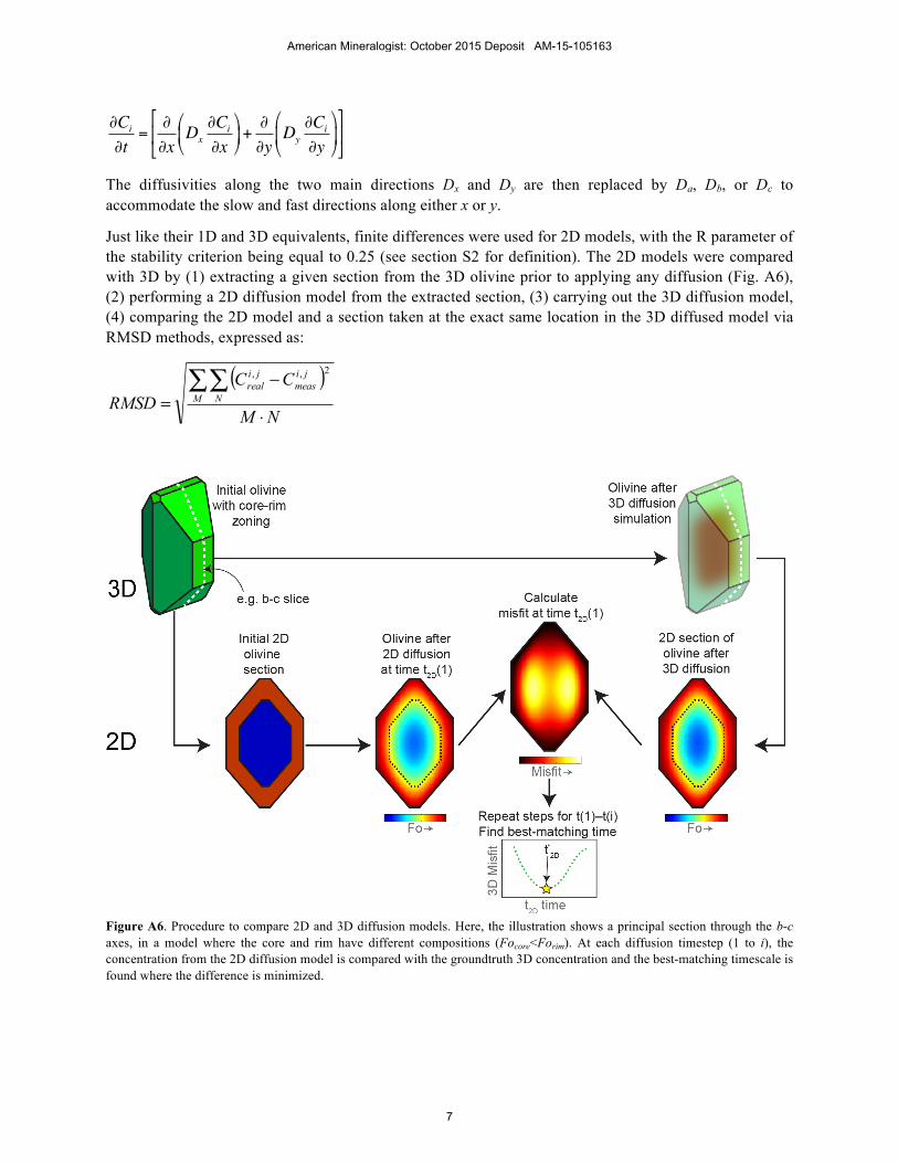
Just like their 1D and 3D equivalents, finite differences were used for 2D models, with the R parameter of the stability criterion being equal to 0.25 (see section S2 for definition). The 2D models were compared with 3D by (1) extracting a given section from the 3D olivine prior to applying any diffusion (Fig. A6), (2) performing a 2D diffusion model from the extracted section, (3) carrying out the 3D diffusion model, (4) comparing the 2D model and a section taken at the exact same location in the 3D diffused model via RMSD methods, expressed as:

( )NM

CCRMSD M N

jimeas

jireal

⋅

−=

∑∑ 2,,

Figure A6. Procedure to compare 2D and 3D diffusion models. Here, the illustration shows a principal section through the b-c axes, in a model where the core and rim have different compositions (Focore<Forim). At each diffusion timestep (1 to i), the concentration from the 2D diffusion model is compared with the groundtruth 3D concentration and the best-matching timescale is found where the difference is minimized.


7

M and N are the number of points or pixels in the x and y directions, i and j are the coordinates, Creal is the ‘real’ concentration taken from the 3D model, and Cmeas is the concentration measured in the 2D model. The best-matching timescale *

2Dt was calculated from the 2D model time yielding the minimum RMSD.

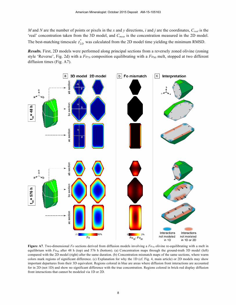
Results. First, 2D models were performed along principal sections from a reversely zoned olivine (zoning style ‘Reverse’, Fig. 2d) with a Fo70 composition equilibrating with a Fo80 melt, stopped at two different diffusion times (Fig. A7).

Figure A7. Two-dimensional Fo sections derived from diffusion models involving a Fo70 olivine re-equilibrating with a melt in equilibrium with Fo80 after 48 h (top) and 576 h (bottom). (a) Concentration maps through the ground-truth 3D model (left) compared with the 2D model (right) after the same duration. (b) Concentration mismatch maps of the same sections, where warm colors mark regions of significant difference. (c) Explanation for why the 1D (cf. Fig. 4, main article) or 2D models may show important departures from their 3D equivalent. Regions colored in blue are areas where diffusion front interactions are accounted for in 2D (not 1D) and show no significant difference with the true concentration. Regions colored in brick-red display diffusion front interactions that cannot be modeled via 1D or 2D.


8

At shorter durations 3Dt = 48 h, the 2D models performed using a-b and b-c sections are identical to their 3D equivalents, while those that used a-c show large concentration mismatches near the edge of the crystal, parallel to [001] (Fig. A7a). If instead of examining the concentration difference between 3D and 2D simulations after 48 h, the best matching time at which concentration differences are minimized are calculated, we obtain *

2Dt = 48 h, 48 h, and 69 h across a-b and b-c and a-c respectively. For longer

durations ( 3Dt = 576 h), 2D-3D concentration mismatches worsen significantly, this time appearing in the three section categories (Fig. A7b). Concentration differences up to ~1% Fo are observed close to the

( )010 and ( )010 faces across a-b and b-c sections, while within a-c sections, mismatches are focused

parallel to c but also measurable in most of the crystal. As before, if instead of tracking the concentration difference with time, the 2D models are run to find the best matching times, we obtain *

2Dt = 712 h, 642 h, and 904 h across a-b and b-c and a-c respectively, systematically higher than the true time.

In a second stage, 2D runs were performed along the same principal sections using the six zoning styles examined (cf. Fig. 2d) and compared against 3D models performed for ‘true’ durations 3Dt = 3, 6, 12, 24, 48, 72, 144, 288 and 576 h. An additional set of 1D models with the same zoning characteristics were also performed for comparison. Best-matching times were calculated, and the time mismatch is here expressed

as a ratio *1

3

Dt

D

trt

= or *2

3

Dt

D

trt

= between the best fit 1D or 2D diffusion times ( *1Dt and *

2Dt ) and the known

3D model duration 3Dt . Value of rt larger than one therefore imply that 1D or 2D overestimate 3D times and vice-versa.

The 1D models along c or b typically match the true 3D diffusion times well (i.e. rt~1), but only up to durations ~72-144 h (Fig. A8). For longer durations, calculated 1D models either overestimate 3D simulation times (normal I and II, and reverse zonings, Fig. A8a, b, c) with ratios reaching rt~2.5, or underestimate the 3D times (core-rim II and III zonings, Fig. A8e, f), with rt~0.5. The 1D models along a systematically largely overestimate the true times for simple zonings (rt>2, Fig. A8a, b, c) and first overestimate then underestimate true times for more complex zonings (Fig. A8e and f). The core-rim I zoning is an exception, with true times well matched by 1D models regardless of crystallographic axis up to around 144 h, after which both time under- and over-estimates occur (Fig. A8d). The 2D models display very similar behavior, matching the true diffusion times perfectly along a-b or b-c planes up to timescales of 288 h for the simple zoning types (normal I and II, reverse) and the core-rim I zoning (Fig. A8a, b, c and d). For longer durations, the simulations tend to overestimate timescales, as in the 1D models. For the two other core-rim zoning patterns (II and III), the 2D runs yield accurate times up to 72 h, and underestimate the 3D times for longer durations. Except for the core-rim I zoning configuration, a-c sections produce inaccurate times, ratios rt typically ranging from 0.5 to 1.8. Both 1D models along a and 2D models across a-c show maximum mismatch for shorter timescales.


9

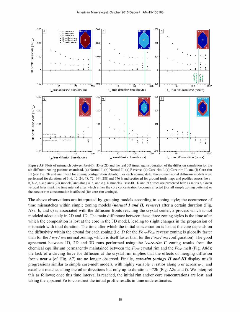
Figure A8. Plots of mismatch between best-fit 1D or 2D and the real 3D times against duration of the diffusion simulation for the six different zoning patterns examined. (a) Normal I, (b) Normal II, (c) Reverse, (d) Core-rim I, (e) Core-rim II, and (f) Core-rim III (see Fig. 2b and main text for zoning configuration details). For each zoning style, three-dimensional diffusion models were performed for durations of 3, 6, 12, 24, 48, 72, 144, 288 and 576 h and sectioned for ground-truth maps and profiles across the a‒b, b‒c, a‒c planes (2D models) and along a, b, and c (1D models). Best-fit 1D and 2D times are presented here as ratios rt. Green vertical lines mark the time interval after which either the core concentration becomes affected (for all simple zoning patterns) or the core or rim concentration is affected (for core-rim zonings).

The above observations are interpreted by grouping models according to zoning style; the occurrence of time mismatches within simple zoning models (normal I and II, reverse) after a certain duration (Fig. A8a, b, and c) is associated with the diffusion fronts reaching the crystal center, a process which is not modeled adequately in 2D and 1D. The main difference between these three zoning styles is the time after which the composition is lost at the core in the 3D model, leading to slight changes in the progression of mismatch with total duration. The time after which the initial concentration is lost at the core depends on the diffusivity within the crystal for each zoning (i.e. D for the Fo70-Fo80 reverse zoning is globally faster than for the Fo75-Fo70 normal zoning, which is itself faster than for the Fo90-Fo70 configuration). The good agreement between 1D, 2D and 3D runs performed using the ‘core-rim I’ zoning results from the chemical equilibrium permanently maintained between the Fo80 crystal rim and the Fo80 melt (Fig. A8d); the lack of a driving force for diffusion at the crystal rim implies that the effects of merging diffusion fronts near a (cf. Fig. A7) are no longer observed. Finally, core-rim zonings II and III display misfit progressions similar to simple core-melt models, with highly variable rt ratios along a or across a-c, and excellent matches along the other directions but only up to durations ~72h (Fig. A8e and f). We interpret this as follows; once this time interval is reached, the initial rim and/or core concentrations are lost, and taking the apparent Fo to construct the initial profile results in time underestimates.


10

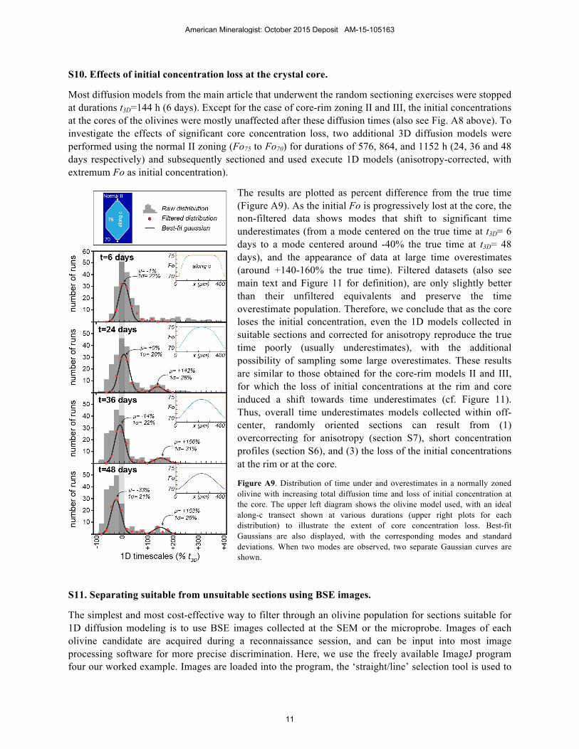
S10. Effects of initial concentration loss at the crystal core.

Most diffusion models from the main article that underwent the random sectioning exercises were stopped at durations t3D=144 h (6 days). Except for the case of core-rim zoning II and III, the initial concentrations at the cores of the olivines were mostly unaffected after these diffusion times (also see Fig. A8 above). To investigate the effects of significant core concentration loss, two additional 3D diffusion models were performed using the normal II zoning (Fo75 to Fo70) for durations of 576, 864, and 1152 h (24, 36 and 48 days respectively) and subsequently sectioned and used execute 1D models (anisotropy-corrected, with extremum Fo as initial concentration).

The results are plotted as percent difference from the true time (Figure A9). As the initial Fo is progressively lost at the core, the non-filtered data shows modes that shift to significant time underestimates (from a mode centered on the true time at t3D= 6 days to a mode centered around -40% the true time at t3D= 48 days), and the appearance of data at large time overestimates (around +140-160% the true time). Filtered datasets (also see main text and Figure 11 for definition), are only slightly better than their unfiltered equivalents and preserve the time overestimate population. Therefore, we conclude that as the core loses the initial concentration, even the 1D models collected in suitable sections and corrected for anisotropy reproduce the true time poorly (usually underestimates), with the additional possibility of sampling some large overestimates. These results are similar to those obtained for the core-rim models II and III, for which the loss of initial concentrations at the rim and core induced a shift towards time underestimates (cf. Figure 11). Thus, overall time underestimates models collected within off-center, randomly oriented sections can result from (1) overcorrecting for anisotropy (section S7), short concentration profiles (section S6), and (3) the loss of the initial concentrations at the rim or at the core.

Figure A9. Distribution of time under and overestimates in a normally zoned olivine with increasing total diffusion time and loss of initial concentration at the core. The upper left diagram shows the olivine model used, with an ideal along-c transect shown at various durations (upper right plots for each distribution) to illustrate the extent of core concentration loss. Best-fit Gaussians are also displayed, with the corresponding modes and standard deviations. When two modes are observed, two separate Gaussian curves are shown.

S11. Separating suitable from unsuitable sections using BSE images.

The simplest and most cost-effective way to filter through an olivine population for sections suitable for 1D diffusion modeling is to use BSE images collected at the SEM or the microprobe. Images of each olivine candidate are acquired during a reconnaissance session, and can be input into most image processing software for more precise discrimination. Here, we use the freely available ImageJ program four our worked example. Images are loaded into the program, the ‘straight/line’ selection tool is used to


11

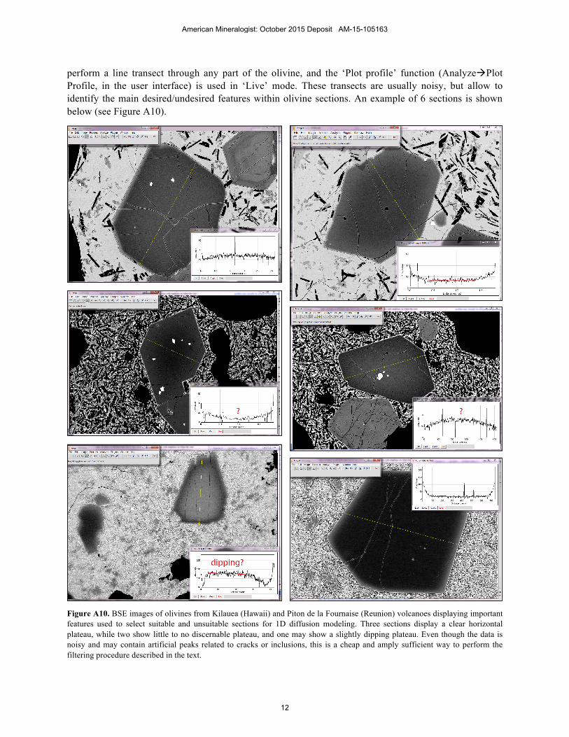
perform a line transect through any part of the olivine, and the ‘Plot profile’ function (AnalyzeàPlot Profile, in the user interface) is used in ‘Live’ mode. These transects are usually noisy, but allow to identify the main desired/undesired features within olivine sections. An example of 6 sections is shown below (see Figure A10).

Figure A10. BSE images of olivines from Kilauea (Hawaii) and Piton de la Fournaise (Reunion) volcanoes displaying important features used to select suitable and unsuitable sections for 1D diffusion modeling. Three sections display a clear horizontal plateau, while two show little to no discernable plateau, and one may show a slightly dipping plateau. Even though the data is noisy and may contain artificial peaks related to cracks or inclusions, this is a cheap and amply sufficient way to perform the filtering procedure described in the text.


12

S1. Diffusion anisotropy corrections - SOEST · S1. Diffusion anisotropy corrections ... more...

Documents

Transcript of S1. Diffusion anisotropy corrections - SOEST · S1. Diffusion anisotropy corrections ... more...