State Transition, Balancing, Station Keeping, and Yaw Control

for a Dynamically Stable Single Spherical Wheel Mobile Robot

Umashankar Nagarajan, Anish Mampetta, George A. Kantor and Ralph L. Hollis

Abstract— Unlike statically stable wheeled mobile robots,dynamically stable mobile robots can have higher centers ofgravity, smaller bases of support and can be tall and thinresembling the shape of an adult human. This paper concernsthe ballbot mobile robot, which balances dynamically on asingle spherical wheel. The ballbot is omni-directional and canalso rotate about its vertical axis (yaw motion). It uses a triadof legs to remain statically stable when powered off. This paperpresents the evolved design with a four-motor inverse mouse-ball drive, yaw drive, leg drive, control system, and resultsincluding dynamic balancing, station keeping, yaw motion whilebalancing, and automatic transition between statically stableand dynamically stable states.

I. INTRODUCTION

Design and control of dynamically stable mobile robots

is a growing area of research. Conventional statically stable

mobile robots generally have large and heavy bases to ensure

low centers of gravity, making them ill-suited for navigation

in human environments. Robots for operation in human

environments ideally should be tall and thin. These attributes

can best be achieved with dynamic stability.

One of the first two-wheeled inverse pendulum type mo-

bile robot was designed and controlled in [1]. The Segway

RMP two-wheeled self-balancing mobile robot base has been

a popular platform in recent years [2]. Very capable two-

wheeled mobile manipulators have been introduced [3]. Such

two-wheeled balancing platforms have dominated the field

of dynamically stable mobile robots but they have kinematic

constraints that restrict their direction of motion. In 2005, the

authors’ group introduced the ballbot, a dynamically stable

mobile robot moving on a single spherical wheel [4], [5],

and popularized in [6]. The single spherical wheel provides

omnidirectional motion making the ballbot more suitable for

navigation in human environments with constrained spaces.

Moreover, unlike its two-wheeled counterparts, the ballbot

is as tall as an adult human, which enhances its ability

to interact with human environments. Recently, others have

developed similar robots [7], [8].

This paper presents an evolved version of the ballbot

with a four-motor inverse mouse-ball drive, a yaw drive that

provides rotation about its vertical axis and a leg drive that

enables controlled transition from statically stable state (SSS)

to dynamically stable state (DSS) and vice versa. Design

details are given in Sec. II. Section III provides a simplified

This work is supported by NSF Grants IIS-0308067 and IIS-0535183.The authors are with The Robotics Institute, Carnegie Mellon

University, Pittsburgh, PA 15213, USA umashankar@cmu.edu,

kantor@ri.cmu.edu and rhollis@cs.cmu.edu

Fig. 1. Ballbot: (a) statically stable, (b) dynamically stable.

ballbot dynamic model, with parameter measurements pre-

sented in Sec. IV. Section V describes an improved, robust

balancing and station keeping controller, yaw controller, leg

controller and an automatic procedure for transition between

SSS and DSS and vice versa. Sections VI and VII present

the results and conclusions.

II. SYSTEM DESCRIPTION

A. Four-Motor Inverse Mouse-Ball Drive

The previous version of the inverse mouse-ball drive [5],

had a pair of drive and opposing passive rollers for each

of the orthogonal motion directions. With this scheme, the

drive rollers produced an upward or downward force on

the urethane-covered ball in addition to torque. This setup,

while operable, resulted in unequal friction for forward and

backward motion in addition to some undesirable “hopping

motion.” To avoid this, the present design has all four rollers

actuated with individual DC servomotors which exert pure

torques on the ball. Figure 2(a) illustrates the main features

of this arrangement.

B. Yaw Drive

The ball drive mechanism is attached to the body using

a large thin-section bearing which allows yaw rotation. The

yaw drive shown in Fig. 2(b) has a DC servomotor with

planetary gears driving the pulley assembly at the center.

An absolute encoder attached to the pulley assembly gives

2009 IEEE International Conference on Robotics and AutomationKobe International Conference CenterKobe, Japan, May 12-17, 2009

978-1-4244-2789-5/09/$25.00 ©2009 IEEE 998

Fig. 2. Four-motor inverse mouse-ball drive and yaw drive: (a) viewshowing main drive arrangement, (b) view showing yaw drive mechanism.

the orientation of the body frame with respect to the ball

drive unit. A slip ring assembly for drive motor currents and

encoder signals permits unlimited yaw rotation.

C. Leg Drive

Fig. 3 shows snapshots of the leg drive mechanism. Each

0.48 m leg is driven by a linear screw drive with a ratio

of 1.6 mm/revolution. The tip of the leg has a hoof switch

and a ball castor. The hoof switch indicates contact with

the floor and the ball caster allows some horizontal rolling

motion along the floor. A spring and linear guide between

the leg and the hoof adds some compliance. The legs are

independently driven by three DC servomotors with 500 cpr

encoders.

III. PLANAR SIMPLIFIED BALLBOT MODEL

The ballbot is modeled as a rigid cylinder on top of a

rigid sphere. The ballbot dynamics are simulated and control

strategies are tested using this planar model. The following

assumptions are made: (i) there is no slip between the ball

and the floor, (ii) motion in the median sagittal plane and

median coronal plane is decoupled, and (iii) the equations

of motion in these two planes are identical. With these

assumptions a pair of decoupled, independent controllers that

stabilize the 3D system can be designed.

Euler-Lagrange equations are used to derive the dynamic

equations of motion of the planar ballbot model shown in

Fig. 3. Leg drive: (a) Various components of the leg drive mechanism, (b)legs completed retracted, and (c) legs completely deployed.

Fig. 4. Planar simplified ballbot model.

Fig. 4. It is to be noted that the model described below

uses a coordinate scheme different from the one described

in [5]. The coordinate scheme shown in Fig. 4 avoids the

coupling between the two generalized coordinates unlike the

coordinate scheme in [5]. Moreover, the coordinate scheme

described here give direct sensor outputs on the real robot.

The generalized coordinate vector of the system is defined

as q = [θ ,φ ]T . The Euler-Lagrange equations of motion for

the simplified planar ballbot model are:

d

dt

∂L

∂ q−

∂L

∂q=

[

τ0

]

−

[

Dcsgn(θ )+ Dvθ0

]

, (1)

where L is the Lagrangian, τ is the torque applied between

the ball and the body in the direction normal to the plane, Dc

is the coulomb friction and Dv is the viscous damping friction

between the ball and the four rollers, 3 support balls and the

ground as well as the motor back-EMFs. The equations of

motion can be re-written in matrix form as follows:

M(q)

[

θφ

]

+C(q, q)+ G(q)+ D(q) =

[

τ0

]

, (2)

999

where M(q) is the mass matrix, C(q, q) is the vector of

coriolis and centrifugal forces and G(q) is the vector of

gravitational forces.

The mass matrix is given by:

M(q) =

[

α α + β cosφα + β cosφ α + γ + 2β cosφ

]

, (3)

where α = Iball + (mball + mbody)r2, β = mbodyrℓ and γ =

Ibody + mbodyℓ2. I and m refer to the moment of inertia and

mass of the subscripted components respectively, while, r,

ℓ and g are the radius of the ball, position of the center of

mass of the body along the vertical axis, and acceleration

due to gravity, respectively.

The vector of coriolis and centrifugal forces is given by:

C(q, q) =

[

−β φ2 sinφ−β φ2 sinφ

]

(4)

and the vector of gravitational forces is given by:

G(q) =

[

0

−β g sinφ

r

]

. (5)

The state vector is defined to be x = [qT qT ]T and the input

is defined to be u = τ . Therefore, Eq. (2) can be re-written

of the form x = f (x,u).

TABLE I

SYSTEM PARAMETERS

Parameter Symbol Value

Z-axis CM from ball center l 0.69 m

Ball radius r 0.106 m

Ball mass mball 2.44 kg

Ball inertia Iball 0.0174 kgm2

Roll moment of inertia about CM Icmxx 12.59 kgm2

Pitch moment of inertia about CM Icmyy 12.48 kgm2

Yaw moment of inertia about CM Icmzz 0.66 kgm2

Body mass mbody 51.66 kg

Coulomb friction torque Dc 4.39 Nm

Viscous damping friction coefficient Dv 0.17 Nms/rad

IV. PARAMETER ESTIMATION EXPERIMENTS

To instantiate the mathematical model, off-line experi-

ments were conducted to determine principal system param-

eters.

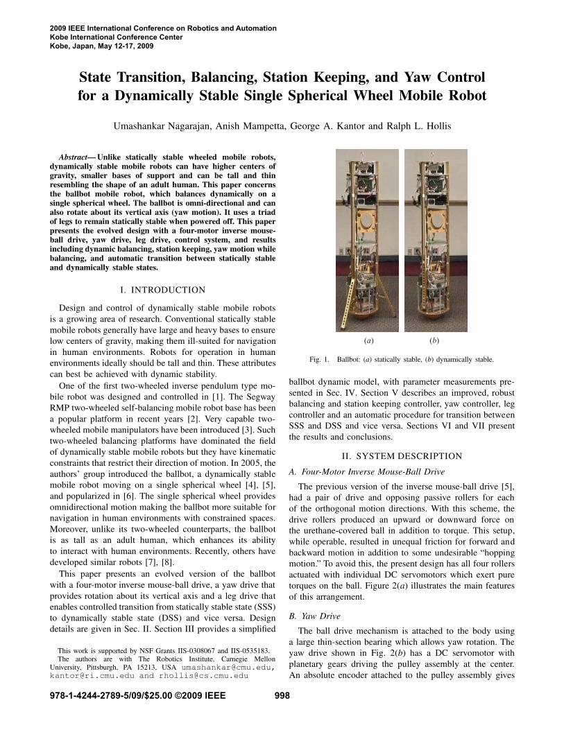
A. Inertia Measurement

Moments of inertia of the body were experimentally de-

termined using a torsional pendulum setup [9]. The ballbot’s

body was suspended about its center of mass using a torsional

spring as shown in Fig. 5 and the oscillations were observed

after an initial disturbance. The body angles were recorded

using the IMU to find the frequency of oscillations as shown

in Fig. 6. The torsional spring constant was obtained by

performing the same experiment with an I-beam whose

inertia was known. The torsional spring constant is given

by

K = Iω2n , (6)

Fig. 5. Torsional pendulum setup with ballbot suspended perpendicular toits length.

Fig. 6. Damped sinusoidal oscillation used to determine the ballbot’smoments of inertia.

where I is the inertia of the suspended object and ωn is the

natural frequency of oscillations. Therefore, the moment of

inertia of the body about its center of mass is given by

Icmbody = Icm

I−beam

ω2I−beam

ω2body

. (7)

Similar experiments determined Icmzz about the vertical axis

by hanging the ballbot vertically. The measured inertia values

are shown in Table I. The moments of inertia of the body

Ixx and Iyy about the center of the ball were computed using

the parallel-axis theorem.

B. Friction Modeling

The coulomb and viscous friction terms were determined

experimentally by standing the ballbot on a roller ball with

its body constrained vertically as shown in Fig. 7. A ramp

current (torque) input was given to the ball while recording

the angular velocity of the ball. The experiment was repeated

with the torque vector at 5◦ intervals. A polar plot of the

breakaway current is shown in Fig. 8. The average breakaway

current provided the value of coulomb friction. The plot of

Fig. 7. Ball rolling on the roller during friction tests,

1000

Fig. 8. Polar plot of the breakaway current in different directions of motion.

0 5 10 15 200

0.5

1

1.5

2

Time (s)

Ba

ll A

ng

ula

r V

elo

city (

rad

/s)

Fig. 9. Linear variation of the ball velocity after breakaway

velocity vs. time after breakaway shown in Fig. 9 can be

approximated by a line of constant slope for small speeds.

The slopes of the velocity plot and the ramp input were used

to determine the viscous friction [10] as shown in Table I.

V. BALLBOT CONTROL

A. Balancing

Balancing for the 3D ballbot system uses two independent

controllers operating one in each of the vertical planes. These

controllers attempt to move the center of the ball directly

below the body center of mass. Each is a Proportional-

Integral-Derivative (PID) controller whose gains were tuned

manually. The control system block diagram is shown in the

shaded part of Fig. 10. The balancing controller takes the

desired body angle φd as input (zero for standing still) and

tries to balance about that angle. One can feed in desired

angles to the balancing controller to move the ballbot around

as shown in a companion paper [11].

B. Station Keeping

The balancing controller is good at balancing about zero

body angles but does not bother about the ball’s position on

Fig. 10. Block diagram for the station keeping controller with the balancingcontrol block.

Fig. 11. Block diagram of the yaw controller.

Fig. 12. Top view of the ballbot with all three legs deployed.

the floor. Station keeping is the act of balancing at a desired

position even when disturbed. The station keeping controller

is achieved with an outer loop around the balancing con-

troller as shown in Fig. 10. It is a Proportional-Derivative

(PD) controller that outputs desired body angles depending

on the error between the ball’s current and desired positions.

The angle output from the PD controller is saturated to avoid

large lean angles. Gains were tuned manually. This controller

replaces the LQR controller of [5].

C. Yaw Control

The yaw drive mechanism has an independent controller

decoupled from the balancing control for simplicity and ease

of control, as shown in Fig. 11. There are two loops: an inner

Proportional-Integral (PI) control loop that feeds back the

yaw angular velocity ψ and an outer PD control loop that

feeds back both the yaw angle ψ and yaw angular velocity.

The desired angular velocity output from the PD controller

is saturated to avoid high angular velocities which could

potentially drive the system unstable while balancing.

During yaw motion, the IMU attached to the body frame

rotates while the ball drive unit does not. The angle offset χbetween the drive unit and the body frame is given by the

absolute yaw encoder. This requires a rotation transformation

to be performed to obtain the roll and pitch angles about the

ball drive coordinate frame as shown below:[

rolldrive

pitchdrive

]

=

[

cosχ −sinχsinχ cosχ

][

rollbody

pitchbody

]

. (8)

D. Leg control

The three legs have independent controllers for lifting the

legs up and putting them down. The legs-up controller is a

PI speed controller that stops when the legs hit the body,

i.e. when the leg speed is less than a defined low threshold

speed. The legs-down controller has an inner PI control loop

1001

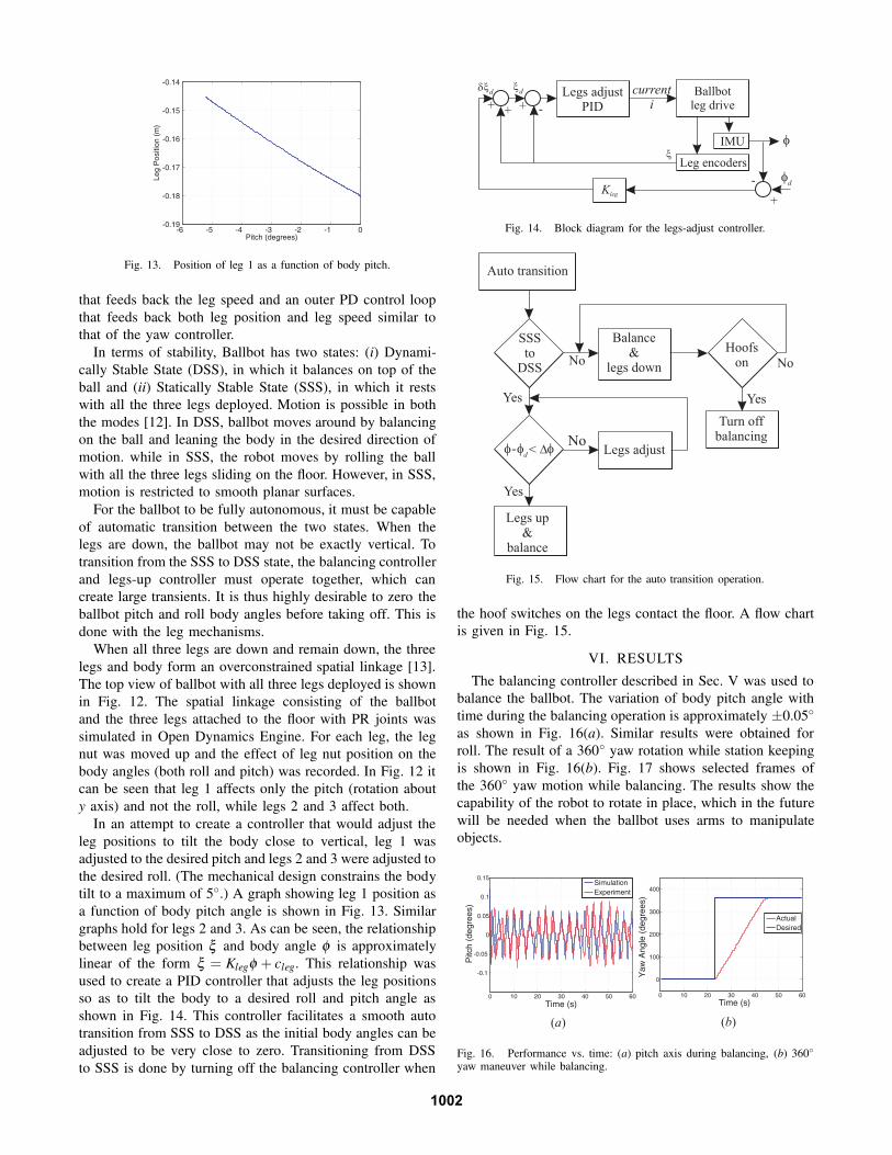
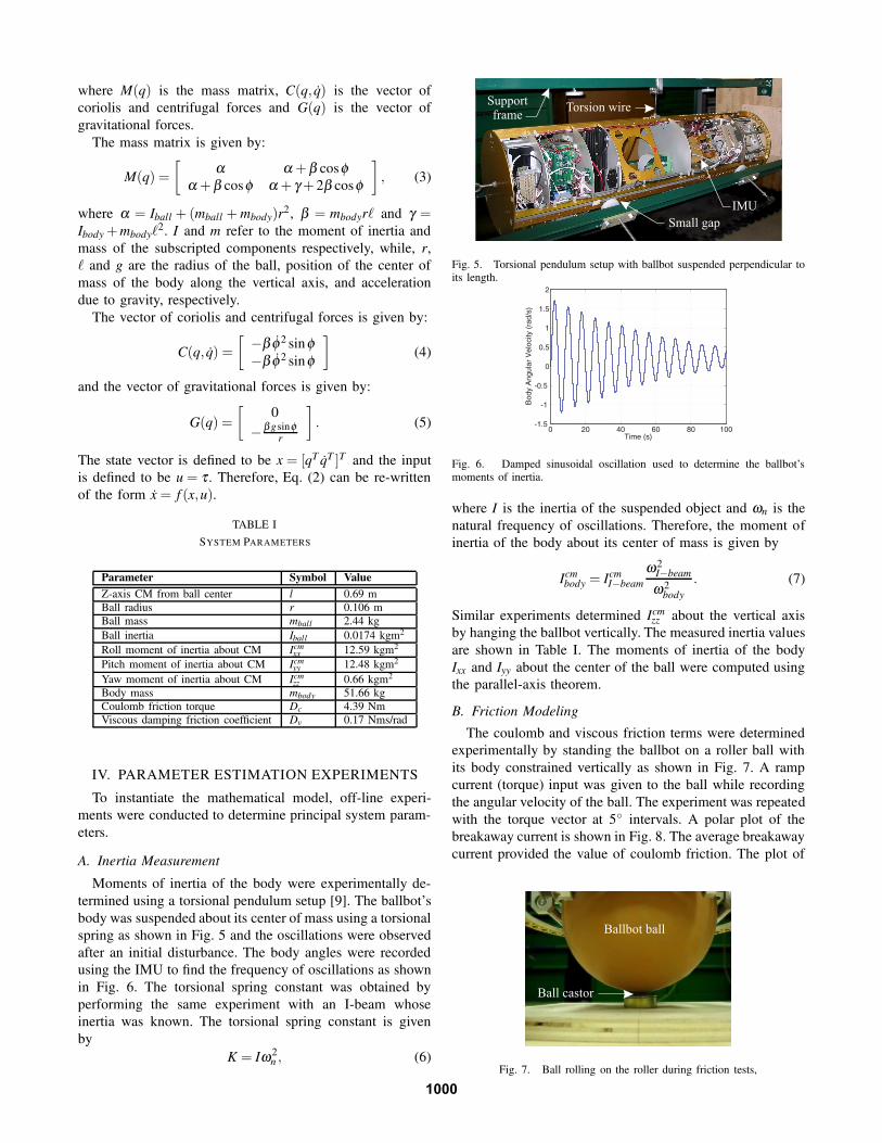
Fig. 13. Position of leg 1 as a function of body pitch.

that feeds back the leg speed and an outer PD control loop

that feeds back both leg position and leg speed similar to

that of the yaw controller.

In terms of stability, Ballbot has two states: (i) Dynami-

cally Stable State (DSS), in which it balances on top of the

ball and (ii) Statically Stable State (SSS), in which it rests

with all the three legs deployed. Motion is possible in both

the modes [12]. In DSS, ballbot moves around by balancing

on the ball and leaning the body in the desired direction of

motion. while in SSS, the robot moves by rolling the ball

with all the three legs sliding on the floor. However, in SSS,

motion is restricted to smooth planar surfaces.

For the ballbot to be fully autonomous, it must be capable

of automatic transition between the two states. When the

legs are down, the ballbot may not be exactly vertical. To

transition from the SSS to DSS state, the balancing controller

and legs-up controller must operate together, which can

create large transients. It is thus highly desirable to zero the

ballbot pitch and roll body angles before taking off. This is

done with the leg mechanisms.

When all three legs are down and remain down, the three

legs and body form an overconstrained spatial linkage [13].

The top view of ballbot with all three legs deployed is shown

in Fig. 12. The spatial linkage consisting of the ballbot

and the three legs attached to the floor with PR joints was

simulated in Open Dynamics Engine. For each leg, the leg

nut was moved up and the effect of leg nut position on the

body angles (both roll and pitch) was recorded. In Fig. 12 it

can be seen that leg 1 affects only the pitch (rotation about

y axis) and not the roll, while legs 2 and 3 affect both.

In an attempt to create a controller that would adjust the

leg positions to tilt the body close to vertical, leg 1 was

adjusted to the desired pitch and legs 2 and 3 were adjusted to

the desired roll. (The mechanical design constrains the body

tilt to a maximum of 5◦.) A graph showing leg 1 position as

a function of body pitch angle is shown in Fig. 13. Similar

graphs hold for legs 2 and 3. As can be seen, the relationship

between leg position ξ and body angle φ is approximately

linear of the form ξ = Klegφ + cleg. This relationship was

used to create a PID controller that adjusts the leg positions

so as to tilt the body to a desired roll and pitch angle as

shown in Fig. 14. This controller facilitates a smooth auto

transition from SSS to DSS as the initial body angles can be

adjusted to be very close to zero. Transitioning from DSS

to SSS is done by turning off the balancing controller when

Fig. 14. Block diagram for the legs-adjust controller.

Fig. 15. Flow chart for the auto transition operation.

the hoof switches on the legs contact the floor. A flow chart

is given in Fig. 15.

VI. RESULTS

The balancing controller described in Sec. V was used to

balance the ballbot. The variation of body pitch angle with

time during the balancing operation is approximately ±0.05◦

as shown in Fig. 16(a). Similar results were obtained for

roll. The result of a 360◦ yaw rotation while station keeping

is shown in Fig. 16(b). Fig. 17 shows selected frames of

the 360◦ yaw motion while balancing. The results show the

capability of the robot to rotate in place, which in the future

will be needed when the ballbot uses arms to manipulate

objects.

Fig. 16. Performance vs. time: (a) pitch axis during balancing, (b) 360◦

yaw maneuver while balancing.

1002

Fig. 17. Selected frames of 360◦ yaw motion video.

Fig. 18. Balancing at a position: (a) ball track on the carpeted floor usingonly the balancing controller, (b) operation of the station keeping controllerwhen the body is pushed off its position.

Fig.18(a) is an XY plot of the ball position on a carpeted

floor. As one can see, the balancing controller is able to keep

the ball close to its starting point on floor to within about

±10-15 mm. Unlike the balancing controller, the station

keeping controller described in Sec. V keeps the ball close to

its starting point even when disturbed. Results of when the

body is pushed by the hand in all four directions is shown

in Fig. 18(b).

Finally, Fig. 19 shows selected frames of automatic tran-

sition from SSS to DSS and vice versa, taken from a com-

panion video “Dynamically Stable Single-Wheeled Mobile

Robot: Ballbot.”

VII. CONCLUSION

A balancing controller was designed to stabilize the single

spherical wheeled dynamically stable mobile robot. A station

keeping controller was designed as a wrapper around the

balancing controller to enable balancing at a fixed location

in the presence of external disturbances. These controllers

were found to be more robust than previously implemented

Fig. 19. Selected frames of automatic transition from SSS to DSS andvice versa.

LQR controllers. Many off-line experiments were performed

to find numerical values for the ballbot’s physical charac-

teristics. Controllers for the yaw and leg drive mechanisms

were designed and implemented. A control procedure for

automatic transition from statically stable state (SSS) to dy-

namically stable state (DSS) and vice versa was designed and

tested on the ballbot. The implementation of the controllers

and their successful and robust operation on the ballbot has

been demonstrated.

The work to date opens up a wide range of possibilities

for ballbot’s actions. The authors have ongoing research on

motion planning and control for ballbot which is discussed

in a companion paper [11]. With these considerations, it

is reasonable to believe the ballbot represents a new class

of wheeled mobile robots capable of agile, omni-directional

motion.

ACKNOWLEDGEMENTS

The authors wish to thank Eric Schearer, Kathryn Rivard,

Suresh Nidhiry, Jun Xian Leong, Jared Goerner, and Tom

Lauwers for their superb efforts on the ballbot project.

REFERENCES

[1] Y.-S. Ha and S. Yuta. Indoor navigation of an inverse pendulum typeautonomous mobile robot with adaptive stabilization control system.In Experimental Robotics IV, 4th Int’l. Symp., pages 529–37, 1997.

[2] H. G. Nguyen, J. Morrell, K. Mullens, A. Burmeister, S. Miles,N. Farrington, K. Thomas, and D. Gage. Segway robotic mobilityplatform. In SPIE Proc. 5609: Mobile Robots XVII, Philadelphia, PA,October 2004.

[3] P. Deegan, B. Thibodeau, and R. Grupen. Designing a self-stabilizingrobot for dynamic mobile manipulation. Robotics: Science and

Systems - Workshop on Manipulation for Human Environments, 2006.[4] Tom Lauwers, George Kantor, and Ralph Hollis. One is enough! In

Proc. Int’l. Symp. for Robotics Research, San Francisco, October 12-15 2005. Int’l. Foundation for Robotics Research.

[5] T. B. Lauwers, G. A. Kantor, and R. L. Hollis. A dynamically stablesingle-wheeled mobile robot with inverse mouse-ball drive. In Proc.Int’l. Conf. on Robotics and Automation, Orlando, FL, May 15-192006.

[6] Masaaki Kumagai and Takaya Ochiai. Development of a robotbalancing on a ball. International Conference on Control, Automationand Systems, 2008.

[7] Laszlo Havasi. ERROSphere: an equilibrator robot. International

Conference on Control and Automation (ICCA2005), pages 971–976,June 27-29 2005.

[8] H. Wang and et al. An experimental method for measuring the momentof inertia of an electric power wheelchair. Proc. 29th Annual Int’l.

Conf. of IEEE EMB, pages 4798–4801, 2007.[9] R. Kelly, J. Llamas, and R. Campa. A measurement procedure for

viscous and coulomb friction. IEEE Transactions on Instrumentation

and Measurement, 49(4):857–861, 2000.[10] Umashankar Nagarajan, George Kantor, and Ralph Hollis. Trajectory

planning and control of an underactuated dynamically stable singlespherical wheeled mobile robot. Proc. IEEE Int’l. Conf. on Robotics

and Automation, May 2009.[11] A.K. Mampetta. Automatic transition of ballbot from statically stable

state to dynamically stable state. Master’s thesis, Carnegie MellonUniversity, Pittsburgh, PA, 2006. Report CMU-RI-TR-01-00.

[12] S. Tsai, E. Ferreira, and C. Paredis. Control of the gyrover: A single-wheel gyroscopically stabilized robot. In IEEE/RSJ Int’l Conf. on

Intelligent Robots and Systems (IROS’99), October 1999.

1003