I(1I

o0•: NAVAL POSTGRADUATE SCHOOL__ Monterey, California

I •) STATrS

DTISS ELECTENOV 05 19939

ATHESIS

PROB1ABILITY OF DETECTION CALCULATIONS USINGMATLAB

by

Wei Yung-Chung

June 1993

Thesis Advisc-w: Gumam S. Gill

Approved for oublic release; distviitUion a• unin:uici.

93-27117- - I~lII , ,, !. =! |•I 01

form Approved

REPORT DOCUMENTATION PAGE oFB o A 7prove8

P; .,1.c "o=r1,nq b.t'e' fO, tPf c O% o f, nfo- 4110-%' t' rt l.t to a-eraqc I oot Df,C'•imte -n(livd.t the time for v'we-C.tq ' %ealtchnq e ,t- q Cat# ,Ourcei

A the, Jq 41 wfa-.h-q the data •eI•d"I " cmi m anf , e1 nd• m e the (aIIf#(t,• Of AfinOli'8O Send (o •ent, II f 0141 1 MitQ ll tdcn 1f.rate of Any other 4t14KI Of tr"I

cnIejpCCn I A • .ncl.to n q . uo4i .0' '~d.fo n r• p. | o ,•voh to wjtIv.,1 qton SIeI. Ldredofatr for I "fOrmtoon Oo'ah.ont And fleOG-Ii. 1 IIS ,eHersonoiv.% HMqtIýy S-1t 1204 Af,InfqlOf VA )2202j_)0j and to the Off'U' of IMnqern"eI .t'o S.OUtt rjoe'Oýl RedvC1,O@ P'Ole¶(0704-0188) VV)hr9O O( 2050j

1. AGENCY USE ONI.Y (Leave blank) 2. REPORT DATE I 3. REPORT TYPE AND DATES COVERED

June 1993

4. TITLE AND SUBTITLE S. FUNDING NUMBERS

PROBABILITY OF DETECTION CALCULATIONS USING MATLAB

6, AUTHOR(S)

Wci Yung-Chung

7. PERFORMING ORGANIZATION NAME(S) AND ADDRESS(ES) S. PERFORMING ORGANIZATIONREPORT NUMBER

Naval Postgraduate School

Monterey, CA 93943-5000

"9. SPONSORING/MONITORING AGENCY NIAME(S) AND ADORESS(ES) 10. SPONSORING/MONITORINGAGENCY REPORT NUMBER

II. SUPPLEMENTARY NOTES

The views expressed in this thesis are those of the author and do not reflect theofficial policy or position of the Department of Defense or the US Government

12j. DISTRIBUTION/ AVAILABILITY STATEMENT t2b. DISTRIBUTION CODE

Approved for public release,distribution is unlimited

13. ABSTRACT (Meimum 200words)

A set of highly efficient computer programs based on the Marcum andSwerling's analysis on radar detection has been written in MATLAB to evaluatethe probability of detection. The progj:ams are based on accurate methods unlikethe detectability method whch is based on approximation. This thesis also out-lines radar detection theory and target models as a background.

The goal of this effort is to provide a set of efficient computerprograms for student usage and teacher's aid. Programs are designed to beuser friendly and run on personal computers.

14. SUIBECT TEHMS 15. NUMBER Of PAGES109

16. PRICE CODE

17. SECURITY CLASFICATION 18. SECURITY CLASSIFICATION 19. SECURITY CLASSIFICATION 20. LIMITATION OF AOSTP "CT

OF REPORT OF THIS PAGE nF '.BSTRACT

L_UýCLASS[FIED UNCLASSIFIED . UNCLASSIFIED I

NSN 7540-01-280-5500 Standard Form 298 (Rev 2-89)i *'CICI'bed t1, AN)I 'ld IIItIt

Approved for public release; dis buonis unlimited.

PROBABILITY OF DETECTION CALCULATION USING MATLAB

by

Wei Yung-ChungLieutenant Commander, Chinese NavyB.S., Chinese Navy Academy, 1984

Submitted in partial fulfillmentof the requirements for the degree of

MASTER OF SCIENCE IN EL717TRICAIJ ENGINEERING

from the

NAVAL POSTGRADUATE SCHOOL

June 1993

Author:

iV1 Yung-Chung

Approved by:

G.S. Gill, Thesis Advisor

R. Janaswamy, Second Reader

Michael A. Moi~an, ChairmanDepartment of Electrical and Computer Engineering

ii

ABSTRACT

A set of highly efficient computer programs based on the

Marcum and Swerling's analysis on radar detection has been written

;n MATLAB to evaluate the probability of detection. The programs

are based on accurate methods unlike the detectability method which

is based on approximation. This thesis also outlines radar

,•-ecticn theory and target models as a background.

The goal of this effcrt is to provide a set of efficient

computer programs for student usage and teacher's aid. Programs

are designed to be user friendly and run on personal computers.

.W 9 U., ht -, " -. ,

F Azcesuo, For

ByI ;-1--

11 -'n

I , 7 -

i~i

TABLE OF CONTENTS

I. INTRODUCTION . . . . . . . . . . . . . . . . . . . 1

A. BACKGROUND . . . . . . . . . . . . . . . . . . 1

B. RADAR RECEIVER MODEL ............ ............. 5

1. DESCRIPTION ............... ................. 5

2. ASSUMPTIONS ............... ................. 7

C. RADAR DETECTION PHILOSOPHY ......... .......... S

D OBJECTIVE ............ ................... 12

II. MODELS AND MATHEMATICAL METHODS. ......... 13

A. MARCUM'S (NON-FLUCTUATING) TARGET MODEL . . .. 13

B. SWERLING'S (FLUCTUATING) TARGET MODELS . . .. 20

1. SWERLING CASE 1 AND 2 ......... ............ 20

a. Case 1 Scan-to-Scan with fluctuations of

exponential density function .... ....... 23

b. Case 2 Pulse-to-Pulse fluctuations of

exponential density function .......... .. 26

2. SWERLING CASE 3 AND 4 ....... ............ 29

a. Case 3 Scan-to-Scan fluctuations with a

chi-square density function with four

degrees of freedom ...... ............ 29

b. Case 4 pulse-to-Pulse fluctuations with a

chi-square density funtion with four

degrees of freedo,.. ..... ............ .. 31

iv

3. SEARCH RADAR DETECTION RANGE CALCULATION 33

III. SOFTA'RE DEVELOPME1T . . . . . . . . . . . . 35

A. PROGRAM STRUCTURE ...... ............. .... 35

1. USER'S GUIDE AND INSTRUCTION ... ........ .. 36

2. PRINTING GRAPHICAL OUTPUTS ...... .......... 37

3. PROGRAMS OPTIONS ......... ............. .... 38

B. ALGORITHMS FOR M-S MODELS ...... .......... 44

1. FUNCTION PROGRAM ALGORIT-IMS ... ......... 44

a. Threshold computataion ..... .......... 44

b. Swerling cast 1 algorithm .... ........ 48

c. Swerling case 2 algorithm .... ........ 49

d. Swerling case 3 algorithm ....... ........ 51.

e. Swerling case 4 algorithm .... ........ 53

f. Swerling case 5 algorithm .... ........ 55

2. SOLVING FOR ROUND OFF ERROR ..... ......... 58

3. SOLVING FOR UNDERFLOW AND OVERFLOW ........ .. 60

4. INPUT ARGUMENTS AND OUTPUT DATA ........ 62

IV. RESULTS ................. ..................... 64

A. PROBABILITY OF DETECTION CURVES .......... .. 70

B. THE DETECTION RANGE CURVES ..... .......... 73

C. NUMERICAL DATA OUTPUT FROM PROBABILITY OF

DETECTION PROGRAMS ....... ............... .. 75

V. CONCLUSIONS AND RECOMMENDATIONS .... .......... 76

A. CONCLUSIONS ............ .................. 76

B. RECOMMENDATIONS .......... ................ 76

v

APPENDIX A. GRAM-CHARLIER SERIES ... .......... 78

APPENDIX B. 14ATLAB PROGRAMS ...... ............. 83

LIST OF REFERENCES ............ .................. 101

INITIAL DISTRIBUTION LIST .......... ............... 102

vi

I. INTRODUCTION

A. BACKGROUND

The Marcum-Swerling (M-S) models are the most commonly

used target models in modern radar analysis. The other target

models have also developed over period of time, such as chi-

square (Weinstock), log-normal. However in this thesis only M-

S models will be discussed.

Histrocially, the earliest descriptions of a target were

in terms of a single cross-sectional area value. This quantity

was usually some type of an average cross section over the

aspect angles which the system designer considered most

probable. The approach led the system designers to associate

a single cross-sectional area of unvarying value, with a

target and thus led to the model of a steady-state target.

Following this concept, systems were designed to achieve a

somewhat arbitrarily specified signal-to-noise ratio at some

specified maximun operating range. The inherent basic

assumption was that the required detection capability and

parameter estimation accuracy could be achieved if this goal

was met. The dominant rule of the human observer in early

detection systems tended to make this approach acceptable. As

the requirements on radar systems became more demanding, and

i]1

as automatic processing of radar returns was developed, the

situation underwent a ý_hange. The desire to optimize radar

designs established the need for more precise target models.

The initial work of J.I.Marcum of the RAND Corporation in

the late 1940s applied the work of Rice of the Bell Telephone

Laboratories, relating to steady-state signals immersed in

noise, to the problem of radar signal detection. Marcum

effectively gave a complete treatment to the statistical

problem of a group of constant amplitude signal pulses in the

presence of noise. His work resulted in an evaluation of

previously untabulated functions ard a direct application of

the results to a gamut of problems in automatic detection.

The statistical approach used in Marcum's studies is the basis

for much of the work that followed in the radar detection

area.

The detection of signals resulting from a fluctuating

target is basically different than for signals resulting from

a non-fluctuating target. A requirement remained, therefore,

to produce the same type of analysis and supporting tabulation

of basic functions for a fluctuating target as had been done

by Marcum for the nonfluctuating target. This work was done by

Swerling, in the early 1950s. He extended Marcum's approach by

employing four target models and two different density

functions in conjunction with two extremes of correlation.

Swerling's case 1 and case 2 are the target models which

describe large complex targets, such as aircraft, rain

2

I

clutter, and terrain clutter. They represent two extremes of

correlation, and the statistical model is derivable from the

physical scattering characteristics of such bodies. -t can

also be stated that empIrically derived data on such targets

are in very good agreement with those obtained from the

mathematical model.

At the time Swerling was doing his work, it was realized

that the model suitable for large complex targets would not

give an adequate description of large simple structures. The

problem of selecting a model to describe this type or class of

target is a difficult one to handle directly. There is no

obvious parallel development for it from the scattering

characteristics of a specific body type. The approach

employed was to establish qualitatively the basic statistical

behavior of the target cross sections of interest. Having done

this, a convenient form of distribution was selected.

Swerling picked a class of distributions know as the chi-

square class, which has the exponential density function

distribution as one member By an appropriate selection of a

class parameter, namely, the number of degrees of freedom, the

qualitative properties desired for the distribution associated

with large simple structures was obtained. Swerling's cases 3

and 4 represent targets that behave as if they have four

degrees of freedom and are valid for targets such as rockets,

missiles, and space-based satellites.

Swerling's two classes of density functions evaluated at

3

two extremes of correlation, together with Marcum's constant

target model (case 5), have been the bases of virtually all

radar detection analyses.

Five target models according to Marcum-Swerling scheme are

as follows:

a) Swerling case 1 - The echo pulses received from a

target on any one scan are of constant amplitude throughout

the entire scan but are independent ( uncorrelated ) from scan

to scan. This assumption ignores the etfect of the antenna

beam shape on the echo amplitude. The probability density

function of the radar cross section a is given by the

exponential density function.

w (a, e 0>0

where C is the average radar cross section

b) Swerling case 2 - With the same dansity function as

case 1 but the fluctulations are ipore rapid than in case 1 and

are taken to be independent from pulse to pulse rather than

from scan to scan.

c) Swerling case 3 - The fluctuation is as;Eumed to be

independent from scan to scan, as in case .1, but the

probability density function is given by the chi-square

distribution with four degrees of freedom.

1 K (Kq1-j)K-1 e_(jTO/-O)=40 e-20/-O, (K=2) (2)(K- 1) -j 2

4

d) Swerling case 4 - With the same density function but

the fluctuation is pulse-to-pulse according to Eq(2).

e) Marcum's model (case 5) - With the constant density

function which represents steady-state target.

The probability density function of equation (1), applies

to a complex target consisting of many independent scatterers

of approximately equal echo areas. The probability density

function assumed in case 3 and 4 is more indicative of targets

that can be represented as one large reflector together with

other small reflectors.

There are curves available that can be used to calculate

the probability of detection for each of Swerling cases, but

for parameters between those charted, the designer has to

interpolate. This can be inaccurate sometimes. Therefore it is

convenient and useful to provide accurate programs to

calculate for any parameters needed by the user.

B. RADAR RECEIVER MODEL

1. DESCRIPTION

The typical super heterodyne radar receiver and the

mathematically receiver model is depicted in Fig 1. The

difference between square-law and linear envelope detector is

that a square-law envelope detector is used in the small

signal optimum receiver and a linear envelope detector is used

in the large-signal receiver. For mathematical convenience,

the square-law detector is applied, but the performance cf

5

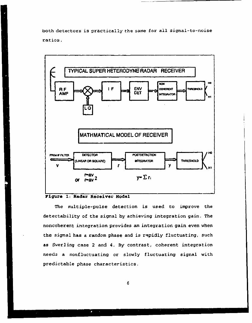
both detectors is practically the same for all signal-to-noise

ratios.

I°

I MAHMAICAL MUE EEODEL OFDA RECEIVER

NON_. HO

"t . HHI

.•o r-av2 y, r

Figure 1: Radar Receiver Model

The multiple-pulse detection is used to improve the

detectability of the signal by achieving integration gain. The

noncoherent integration provides an integration gain even when

the signal has a random phase and is rapidly fluctuating, such

as Swerling case 2 and 4. By contrast, coherent integration

needs a nonfluctuating or slowly fluctuating signal with

predictable phase characteristics.

6

2. ASSUMPTIONS

The assumptions embodied in the M-S detection problems are

as follows:

* A received pulse train consisting of N samples of noise

or signal-plus-noise is available.

0 The signal is imbedded in white Gaussian noise of known

spectral density of N0 /2.

0 The signal is of unknown phase type, where the RF phase

between pulses in the train are randomly distributed.

o The processing consists of a matched filter and square-

law envelope detector which operates on each pulse of the

train and a linear integration which comnbines the n square-law

envelope detected pulse.

* The directivity pattern of the antenna is rectangular so

that the n return pulses resulting during the antenna's dwell

time on the target are unaffected by the antenna's radiation

pattern.

* The target's cross section can be described by a chi-

squared distribution with 2k degree of freedom.

W(o,-) - _ (3)(K-l).! -

C. RADAR DETECTION PHILOSOPHY

Radar detection is complicated by the fact that the target

cross section a is a random variable fluctuating with time and

.7

both noise and clutter. Extraction, or parameter estimation,

is likewise complicated by random fluctuations of the target

echo. For the radar detection case Neyman-Pearson criterion is

used which needs neither a priori probabilities nor cost

estimates. In radar terminology whose objective is to maximize

the probability of detection for a given probability of false

alarm. This objective can be accomplished by using a

likelihood ratio test Specially, there exists some

nonnegative number 71 such that hypothesis H, (i.e.,target is

present) is chosen when

A(y) n(Y) z (4)f(Y)

and hypothesis H0 (no target present) is chosen otherwise.

There are two types of errors which can be made. If we say a

target is present when in fact it is not, an error of the

first kind is made (see Fig 2). That is, we choose H, given

that Hc is true which is denoted as the probability of false

alarm. Similarly an error of the second kind is made when H0

is chosen and in fact H, is true which is probability of miss.

8

Actub(

HO H1

DedaralUon

Correct decision Missing target

HO No target present Error of secondkind

False alarm Correct decisionH1

Error of first kind Target present

Figure 2: Error of detection

To optimally detect the signal with unknown phase,

consider the narrowband signal of duration T given by

s(t) =Aa(t) cos~wot:+O(V) +io]

=szcos#-s'7sin4)

where S,=Aa(t)cos(wot+6(t) ], Sq=Aa(t)sin[wot+O(t) I, A is signal

amplitude, a(t) is an envelope function of duration T, O(t) is

the signal phase modulation. Waveform r(t) is assumed to be

prefiltered by an ideal low-pass filter that is distortionless

within (-w,,w,) and zero outside the interval; therefore the

filter will not affect the band-limited input signal s(t) but

results in a band-limited statistical process. Under this

L9

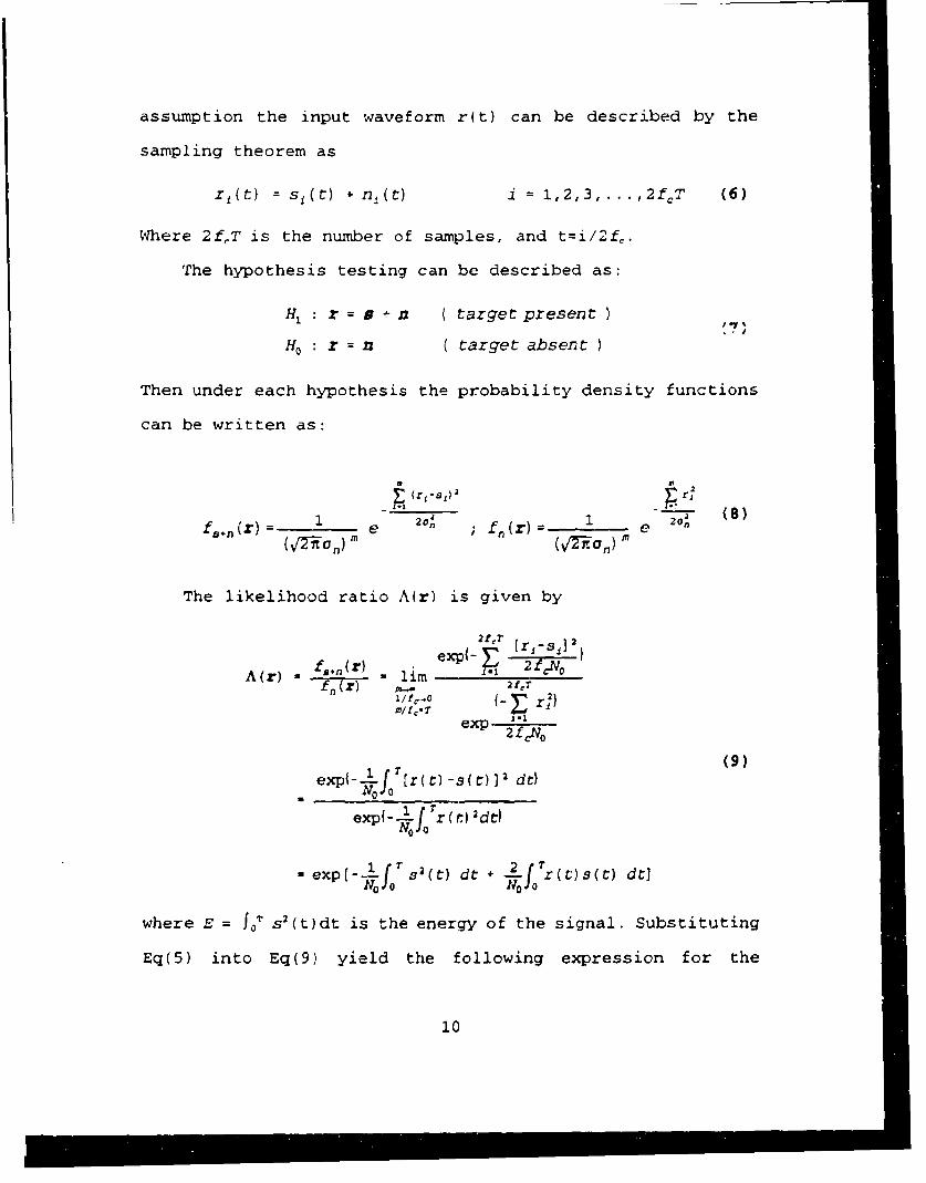
assumption the input waveform r(t) can be described by the

sampling theorem as

r,(t) = s,(t) + n,(t) i = 1,2,3, ,2f.T (6)

Where 2fT is the number of samples, and t=i/2f,.

The hypothesis testing can be described as:

H, : r = a + ( target present)

Ho : z = ( target absent)

Then under each hypothesis the probability density functions

can be written as:

2

2- 1 e 220 ;- e(8)

(v,-,•-on (Z (4 -ra,)

The likelihood ratio A(r) is given by

24Tr [rIsi]2)2f N0expl- 2?f cVA (r) =f,-n~r lim

J 1exp 2f4n°

__ 7 (9)expi-f rr(c) -s (r)] 2 dt)

expl- fo f0z (t) 2dt)

- exp(- 1 - sf2 (t) dt +-f Tr(t)s(t) dt]

where E = ]0T s'(t)dt is the energy of the signal. Substituting

Eq(5) into Eq(9) yield the following expression for the

10

likelihood zatio A(r I

A(rj¢) = exp{- -E [ fT r ( C)s(C)dc]cos4

(10)

- -f [r(t) sq(t)dt]sin¢

Let the signal-to-noise ratio 1 =E/No and

y,(T)= N2 0 TrIf t dt

(11)

using Eq(ll), Eq(10) can be written as follows

A(rIj) = e-f/ 2 exp {Vf[(y(T) coso - yr,(T) sino]}

(12)

= e-9 / 2 exp {VV r(T)cos (4)+a)}

where a=tan-1 (yQl/y) ,r(T)=[yQ(T)+y 1 (T)] 12 is the envelope of the

radar signal out of a filter matched to the waveform (2/No

V'l 2 )s(t), sampled at time t. Assume 0 is a uniformly

distributed density function U(O 2M). Averaging with respect

to 0 yields the averaging likelihood ratio as follows

=e-1'2I0 [2 f r (T) (

where Io(/ 2 rz-(T)) is the modified Bessel function of the first

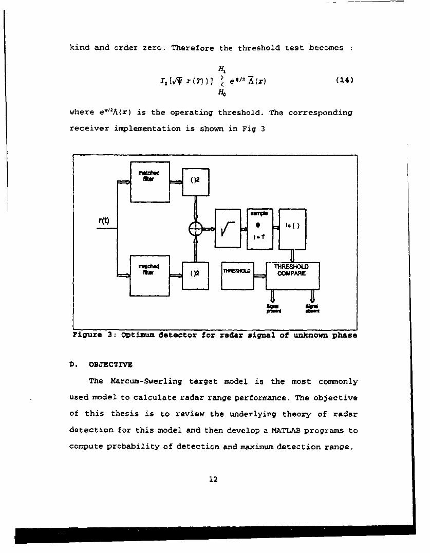
kind and order zero. Therefore the threshold test becomes

I,0[VW -r(71 ] )1 e *11 X(r) (14)

Ho

where ew/ 2A(r) is the operating threshold. The corresponding

receiver implementation is shown in Fig 3

- --

Figure 3: Optimum detector for radar signal of unknown phase

D. OBJECTIVE

The Marcum-Swerling target model is the most commonly

used model to calculate radar range performance. The objective

of this thesis is to review the underlying theory of radar

detection for this model and then develop a MATLAB programs to

compute probability of detection and maximum detection range.

12

II. MODELS AND MATHEMATICAL METHODS

The procedure for the calculation of average probability

of detection P, for Marcum and Swerling cases is as follows:

l)Find the single pulse characteristic function, C1 (p), by

transforming the single pulse probability density function

f,. (y).

2)Find the N pulse characteristic function, CN(p)=[C (p) ]N

3)Average the N pulse characteristic function over the target

distribution to find the average of C,(p) ( 0,(p)).

4)Transform Ce(p) to find the average ensemble probability

density function f,.,(y) and f (y) for the N pulse return.

5)Find probability of false alarm P,. by integrating 4(y)

from Yb to infinity.

6)If Pr. is given find Yb by means of the mathematical

recursive method.

7)Find the average probability cC detection Pd, by integrating

the density function of signal plus noise f,.N(y) from the

threshold Yb to

A. MARCUM'S (NON-FLUCTUATING) STEADY-STATE TARGET MODEL

The non-fluctuating target model is applied to spherical

or nearly spherical objects, such as balloons, many

wavelengths in diameter. The target model, therefore, can be

13

represented by a constant-valued radar cross section.

The Rayleigh and Rician probability density function of

the envelope detected output for N pulses are given by

fnf(r 1iHo) = zier ; r12O

- • - (1 5 )

f.,.ri-IH) = re 2 1 0 (rji4) ; .raO

where 14=E/No is the single pulse peak signal-to-noise ratio

for a steady target. Since the noise received in the ith

observation interval is assumed to be statistically

independent of the noise in every other observation interval,

and the signals are noncoherent between the different

observation interval, the initial phase 01 in Eq(5) in the ith

interval is also statistically independent of Oj for all i#j.

The likelihood ratio test in Eq (9) can be written as:

-- (r 2 r. 1IS M N f (.ris,)

f0(rl]O ) i.i f0 (rf1)

- -] e-/ 21 0 (r1iV ) (16)1-1

-Ne'u)/2 fi] I (r1VW)

From Eq(16), the test statistics is

l1nl0 (r,4) ' e #/2 (~) 17)HO

14

For small signal, the modified Bessel function 1o(x) can be

approximated for x<l as:

0 (x) = 1+ X2 + . . . . . .4 64 (18)

In 1o(X) = x1 (X4 64 4

Therefore Eq(1 7 ) can be rearranged and modified as

NS2 t/ (19)

I-1

where T1 is the operating threshold which is determined by

specifying the false alarm probability.

Marcum utilizes a square law detector law which allows the

signal-plus-noise probability density function to be expressed

directly in the signal-to-noise ratio W. To simplify the

calculation, let

N 2 NY=y 2E -2 q (20)

which Y is compared to a suitably modified threshold Yb

To find the probability density of Y, first the

probability density of fo.n (qd) is found by Jacobain

transformation f 5.. (r,) from Eq(15) into f..(q 1 ) as follows:

-f ir) = e 2 I (I 2--) , q,-o (21)

15

Since random variable Y is the sum of N statistically

independent random variables qi, by applying the relationship

between the sum random variable and the individual random

variable of the characteristic function, and the Campbell and

Foster tables of Fourier transforms ; the C,(p) is

CY (p) =1Cqt (p) = 3i- e •fs.•,%(qý) dqjN N.- . -I.

f - ejPq3 e(/ 2 ) 10 (V2_q-q) dq1 (22)

(l+p) N

From Campbell and Foster Tables of Fourier transforms pair

650.0, the probability density function of f,,,(Y) can be found

by taking the inverse transform of C,(p).

2y (N-2)/12

f'.' (Y) = Y e -''/ 2 IN.(V) ,: >O (23)

For small Y, the modified bessel function I,_ (Y) can be

approached as:

y2 y2 y1+(Y) - [1+ y2 + (24)2m7M! 22 (m+l) 25 (m+l) (m+2)

Therefore the resulting normalized square-law detected

probability density function is

f(y M-e = Y-.N/2(N-I)! ' (25)

16

for noise only the probability of density function f.(Y) is

fn (Y) YN-) e0 (26)

(N- 1)!

A computer simulation of 4 (Y) at the square law detector

output is given in Figure 4:

0.14

0.12

o 0.1-Z.

"•'0.08

S0.06-

. 0.04--0

0.02"

0 10 20 30 40 50 60 70random variable

Figure 4: Simulation of noise at suare law detector output

After square-law detection, the normalized square-law

detected variate (y) is summed over the N-pulses in the pulse

train and thcrn compared against a normalized threshold voltage

(Yb) to determ.i the presence or absence of a target return.

The probability of false alarm can be obtained by

17

integrating from the threshold (Yb) to infinity

f YN-le-Y (27)P. = Jyb ( 1 dY

The incomplete Pearson gamma function which is very useful

for describing M-S model is defined as:

I(u,p) = fv[u(P-.)) e-ydy (28)fo p!

And in term of the Pearson's incomplete gamma function, Eq(27)

is

Pta(NiY•) = I-IYb/NI, (N-i)1 (29)

where U=(y/N"12 ) and P = N-I.

Eq(29) can be successively integrated by parts and given

as:

YM-1) [ (N-1) (N-i)(N-2) ...

(N-i)! (i (30)

N- 1 ybK e- YbK-0 K

The above equation also can be approximated for N>>l by

letting

+ N-I_, (N-i) (N-2) I._]__ N1.

b Yb2 -N-1 (31)

and by applying Stirling's approximation

N! N N (32)

e

The probability of false alarm in Eq(30) can be approximated

18

as

P[6" (N e' N3 (33)Y-b-N+l

The probability of detection for steady-target (case 5)

can be obtain by integrating f from yý to -o and is given

by

PD(Y) = f, 8 .n(Y) dY

(34)

o- 2Yb(..y-) (N-i)/2 e-y-(mv)/21I (VTV) YiOf N-V

The Q function is defined as

, f N-' exp[-( ) +V] IN_,(av) dv (35)WN'UJ ~I2N-

For N pulses the probability of detection PD can be

written in terms of Q function as follows:

PD, (Y) = Q (7 , I V/') (36)

Another approximation can be made by using Gram-Charlier

series expansion ( Appendix A ) and noting that Gaussian

fanily is closed under linear operation.

I= ) dC (p) N(I ;4r/2)

mI k -J dp P.0/

M2 = (-j) 2 d2CY(P) (N2 (141p/2)2+N(1t4137)dp N lp~o N2I /2 + ( + )

o 2 _m2 -i N(1+4)

where mn1 is the ith moment of the distribution of Y and a is

19

, I I I . .... i. .. .. . .. i • I I I I I I I l I I i I I I

the variance of 1'.

V•w.N(J +•) 2N(I+i)y) e Y-Ar'12N(38)f,• (y) a__! e (•-•• ,

Therefore the probability of false alarm can be represented

as:

" (Y-MN -z-Paf 2 f e -2- dZ where Z=- Yb-N

Yb--N Y b - 'V V I cV ~ v I ( 3 9 )

.

Yb can be solved from the above equaticn

Yb V (P4r( ) "-N (40)

The probability of detection can be obtained as

P!;ý a 4t[ (Yt-N(l+T/2) )]( 1

S*--

B. SWERLING'S (FLUCTUATING) TARGET MODELS

1. SWERLING CASES 1 AND 2

The radar cross section of a target (6) is the area of a

hypothetical reflector --hat scatters all radar beam energy it

in-ercepts omnidirectionally, such that it prod-,ces an echo at

the radar antenna equal to that energy actually received from

the target; that is

20

(power received by antenna)(incident power density per 471 rad)

(42)

=lira 4nR 2 -j[2

Where E, is the electric field incident on the target, E4 is

the reflected field as measured at the radar receiver antenna,

and R is the distance from the target to the radar receiver

antenna.

The total electric field received from a complex target

can be expressed as a summation, nan,ely,

ERI- >jrRr exp(2.4 ic -j (43)K-1

and theretore the radar cross set.tion is

a=[ EVFa7 exp(

K-1 (44)

= V/. T -0 T [Cos ( 4 dj ) + j sin ( ---- ) ]1

I wiir re-

4I

a• is the crossing section of individual scattering

elements,

n the number of scattering elements,

dK the range of the Kth element,and

X the wavelength.

In order to reLate the proceeding to a real target two

assumptions shall be made:

21

(1) On a short term basis 4nd,/X is a random

variable which can take on any value from 0 to 2n with equal

probability.

(2) The individual scattering elements have equal

radar cross sections, that is, Ok=o0 .

Therefore the random variables can be expressed as the x

component (CO)d*n2 1cos (41rdk/k) and the y component (CO)"/2

cos (4ndk/%) , the problem of determining the probability

density function of ca is identical to the problem of

determining the distance moved from an origin in a two

dimension walk problem of n steps, where the length of each

step is (C 0 )"12 and the direction of each step is perfectly

random.

The probability of having a component (x,y) after n

steps where n is a comparativity large number is given by

w(x,y) dx dy = exp[-(x 2 +y2 ) /no°] dx dy (45)

Converting from rectangular coordinates to polar coordinates

yields

W(R,O) dRd0 = -R-exp[-(R 2 )/nh 0] dRdO (46)

The marginal distribution of R, obtained by integrating the

preceeding with respect to @,is

w(p) dR = 2 -Rexp[-(R2)/nuo] dR (47)nuo

22

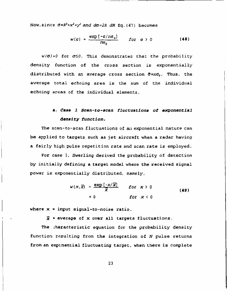
Now, since (7=R2=x2 _yl and da=2R dR Eq. (47) becomes

w(c) = exp[-o/na0 ] for a > 0 (48)noo

w((Y)=O for a50. This demonstrates that the probability

density function of the cross section is exponentially

distributed with an average cross section C=nao. Thus, the

average total echoing area is the sum of the individual

echoing areas of the individual elements.

a. Case I Scan-to-ucan fluctuations of exponential

denalty function.

The scan-to-scan fluctuations of aw exponential nature can

be applied to targets such as jet aircraft when a radar having

a fairly high pulse repetition rate and scan rate is employed.

For case 1, Swerling derived the probability of detection

by initially defining a target model where the received signal

power is exponentially distributed, namely,

w(x, X = exp(--x/lx for x> 0x (49)= 0 for x < 0

where x - input signal-to-noise ratio.

Y * average of x over all targets fluctuations.

The -haracteristic equation for the probability density

function resulting from the integration of N pulse returns

from an expcnential fluctuating target, when there is complete

23

correlation between pulses, is derived from the non-

fluctuating case (Swerling case 5) characteristic function as

follows:

-NxP'

C,--[C,]N= e-mxe P-1Y

(P+l) N-(,(p2j) (50)

1'p+1)N-1 [l+p(l+Nx-)]

For noise only, the characteristic equation is the same as

for case 5.

CN- (51)(1+p)N

The probability density function f,(y) obtained by using

Campbell and Foster 431, p.44, is the same as the probability

density function of the nonfluctuating case. i,e,

-1 e-(52)

(1+N)!

For signal plus noise, the probability density function

f..,(Y) was obtained by using Campbell and Foster pair 581.7,

p.64. For NM>, the density function f,.n (Y) is

24

[-~ ~ J2nPy dp:J (P+1) N- I(1 [+P U+Nx- I

._ e-Y/ iI N.• 1 -FN I - (- l+-- r__y

r (N-1) )N-+Nx-1.NXr• (N -1 , __Y ( 5 3 )

N5 Nx= _Xe.i,. (1+_11)N 1( Y ,N-2)

Nx+ 1

Nx

where F(v,z) i. the incomplete gamma function and I(u,p)is the

incomplete Pearson gamma function.

For N=i, the probability density function can be obtained

from Campbell and Foster pair 438, p.45 as

z.. Y) =e I -ll / (I +x-ý (54)

therefore the probability of detection can be obtained by

integrating Eq(54) from 0 to Yb and the result is given by

Swerling as:

l-•f0Yb f,.,,(y) dv--I( Yb N-21 - (1÷Nx-f (Yb) (55)

From above, PD can be obtained as

V~h1 (56)

2 b N-2) e"5b/ (I *AM11 + ( i/ trx) V7-:£

25

Another approximation can be made by inspecting Eq(56) and

let Ng>>l and Pf<<l such that the Pearson incomplete gamma

functions are close to unity. Then Eq(56) can be rewritten

approximately as

1 e -i-2 Nx.l (57)NIX' 2 Pl 1

Taking the logarithm of Eq(57) and using a series expansion of

each term,

InPa, ( N-1)ln (1+ 1~_ - b

Nxý ( NX- (1+ _)Nx

2(N_) [ 1 _ 1 1 . . (58)(Nx-) 2 (Nx/2)2 3 (NR/2) 3

S[- +N71/2 (NU5•/2 )2 (NVI/2)1

Taking only the first terms and using Eq(40) yields

2ln PDS---L(Yb-N+l)

Nx (59)2--- [V (Pfa) +1]

Nx

b. Case 2 Pulse-to-pulse fluctuations of exponential

density function.

Pulse-to-pulse fluctuations of an exponential nature apply

to targets such as propeller-driven aircraft (if the

propellers contribute a significant portions of the echo

area), to targets where small changes in orientation would

26

establish significant changes in echoing area (such as long

thin subjected to a high-frequency signal), or to targets

viewed by radars with sufficiently low repetition rates.

For case two, the received signal return still belongs to

exponential distribution. For this case the signal is

completely decorrelated (pulse to pulse fluctuations exist),

the probability density function for noise only (signal-to-

noise ratio equals to 0) still the same with Case 1. The

probability of density function of signal plus noise for case

2 can be obtained with the same procedures, but have the pulse

to pulse integration. The characteristic equation for the

single pulse is obtained by letting the characteristic

equation of case 1 to be N=1

C(p) 1 ( (60)

[l +p (1 x-)]

For 1 pulses which is completely decorrelated (independent),

the characteristic equation is just the Nth power of single

pulse

C( ) N1+P(l+x

Therefore the corresponding probability of density

function obtained by using Campbell and Foster "Tables of

Fourier transforms" pair 431, p.44 yield:

27

fe.n(Y) f 1 ]Pe2?•PYdy = y __- e (-6/2)l 1+p (1+X--) (l +X--) (NI)V (

The probability of detection can be expressed as:

P I-ff,. (y) dy

1- (1 f Yt y N-1 e -y/(1÷; dy= -(N-1)! +3F i+3F ( 6 3)

= 1-Ir[ , (N-1)]

Another approximation can be made by applying that the

Gaussian family is closed under linear operation and by using

Gram-Charlier series expansion (Appendix A) so that

mI= (_) dCy(p)dp V0 = N(1+x)

= (j)2 d 2Cy(p) 1P.0 = N(N+l) (l+X)2, (64)dp N

Variance : r= 1

The approximate probability density function then is

fsN(Y) _ 1 eI '

VT -7-cI + x-- (65)

4(Y) -1 e('Y-N/2N

Therefore the probability of detection and false alarm can

be obtained by integrating from the threshold level Yb to

and are represented as:

28

_ [ N( ( 1 ( 66 )

2. SWERLING'S CASE 3 AND 4

For Swerling's case 3 and case 4, the radar cross section

can be described by chi-square distributions with four degrees

of freedom. The density function is commonly associated with

tabilized missile tankage and can be expressed as:

2x

W (X, X--= - 4X e ;F x>0 (67)

a. Case 3 Scan-to-scan fluctuations with a chi-square

density function with four degrees of freedom.

The characteristic equation for case 3 which represents

the c'-ndition of complete correlation (scan-to-scan, no pulse-

to-pulse fluctuation) is given by :

F(P)= f-i4 e 7" (L .- l~'CP+1 i:-t J) e -f =j (68)

2

The characteristic equation and the probability of density

function for noise only remain the same as in case 1 and 2

ip.-l) N (69)

f (Y) -- 7-- 1 eJ 2 79pYdp = yN-1 e-Y

p+ N) • (N-i) !

For signal plus noise the probability of density function

29

can be expressed as:

(P* 1 ) 2-N eJ2XY dp2 ((70)

Y N-1 r0(N-W) [(,+(N 2)2W 1•2N + 2 "N

where the density function comes from Fourier transform pair

581.1 in the Campbell and Foster tables given as

1 ` yI-1 e-(PO)Y1/2 X(s.P p)UV(so)U -v F(2a) (p-o)a (71)

-% ,s-1/2-! (p -() Y] , <0

where

A4,(Z) = Z e F2(pv+2 +,2I1L4+1;Z) (72)

Eq(72) can be simplified using the relationships for the

confluent hypergeometric function, that is

F1 (2,N;Z) = (Z+2-N)F1 (l,N;Z)+N-1

F,(1,N;Z) z e z Z - 'I(N-1) ! I[ Z N-2] (73)

Swerling uses two identities relating to confluent

hypergeometric functions in order to expand the proceeding

into more familiar Pearson's form of the incomplete gamma

function, I(u,p) which is defined in Eq (30), thus Eq (73)

becomes

30

IM I

[, 1+(2 -2 _( Y ,N-2) e(-y/1*(lr/2))

(I+ (NA/-2) ]I2 [ 1 +2 (Nx I VITT

(M-2) [I+ (2/ (AM--1M-1 I[ Y ,N-2] (74)[1+ (Nx-/2)1]2 1i+ (2/Nx7 I] N -

e "y/ (I OR + y N-Ie -y

1I+(NMx/2)] (N-i)

The probability of detection can be obtained by

integrating the density function from the threshold Yb to

as:

yz- eE r2Yb N -2 -P D = + (= e m(N-2)! Nfx+2 M!- Nx

2 yb (75)2 2(N-2) 2Yb -N-2 -2 Yb (----j

Nx Nfx ÷2 I-0 am

b. Case 4 pulse-to-pulse fluct-.4:ns with a chi-

square density function with four degrees of

freedom

With no correlation, the characteristic equation for a

single hit is obtained by letting N=1 in Eq(52)

(P) = (76)

The characteristic equation for the sum of N pulse can be

obtained by the Nth power of a single hit

31

CM(p)=I (p)] N= (13p/)]= - (77)

The inverse Fourier transform of above equation is

obtained from Campbell and Foster transform Pair 581.1,p. 6 4 ,

this yields the following expression for the probability of

density function in the condition of signal plus noise

7C2 e l+p(l+3F/2)]2N- (78)

M1e */2 (N-1) ! F1 (-N,N; -X/2( I +X- 2N 1+3/2y)I

The confluent hypergeometric function F,(-N,N;a) can be

expanded as:

F1 (-N,N;a)=-1 -_N a (-N) (-N.1) a_ (-N) (-N-1) (-N+2) a .......N 1! N(N.1) 2! N(N4I) (N+2) 3! (9)

"N '-1) "(N!/(N-K)!] axS[(N- K- 1) 17(N- 1) 1] KI

From Eq(78) and Eq(79), the density function f1 .,(Y) can be

rewritten as

yN-le 1 2N! E (x/2 K Y (80)

(1 2) K1 F/2 [ (N+K-I) ! (N-K) ! K!]

The probability of detection is obtained by integrating Eq(80)

from the desired threshold Yb to -. From the definition of

incomplete gamma function, the probability of detection can be

32

written as:

P D f., (y) dy

I[ Yb N+K-] (N! K (13F/2) VR/ '

(I+X/2) -0 (2 K! (N-K)!

With Eq(40), the probability of detection can be approximated

as:

I[fN 40T7(Pfa) +NN -I[ -i (P.) , N+K-I] 82N! K (1+'a12) VV17;*(21(i+/2)'D ) K! (N- K)!

c. SEARCH RADAR DETECTION RANGE CALCULATION

The Marcum-Swerling theory represented by extensive sets

of curves from the computer programs can be used to determine

tne detection range of a practical radar by introducing

detection loss and others parameters. There are many types of

detection losses which have been identified so far, and when

these are considered, reasonable predictions of radar

performance can be obtained.

The radar's detection range can be determined by applying

the desired signal-to-noise ratio determined from the Marcum-

Swerling theory and the calculated detection loss, as given by

33

Rm= [ PGtGr1X2 0 J1/4 (M) (83)(4 4R ) 3 kTBjF L

where

R.• = The maximum detection range in meters

Pt= Peak transmitter power in Watts

X = Wavelength in meters

G,,, = Transmitter and receiver antenna power gains

S= Average radar cross section in square meters

k = Boltzmann's constant= 1.38 x 1023 J/deg.

T = Effective system input noise temperature in degrees

Kelvin ( 0 K)

B = Receiver bandwidth in Hertz.

L = Detection system power loss factor

F.= The receiver noise figure

S/N= The smallest output signal-to-noise ratio

When n pulse are integrated previous equation can be

written as

P~ = [ PtGtGr 12an ]I4()(8.MaX Pe 3 1/4Uf (in) (84)(41) 3kTBFL (-ý) n

where the parameters are the same as that of Eq (83) except

that (S/N), is the signal-to-noise ratio of one of the n

pulses that are integrated to produce the required probability

of detection for a specified probability of false alarm.

34

II. SOFTWARE DEVELOPMENT

This chapter describes the development of MATLAB programs

for the efficient and accurate conputation of probability of

detection based on Marcum and Swerling theory of radar

detection. The MATLAB source code is given in Appendix B, and

complete programs are available from Professor G.S. Gill, Code

EC/Gl, Naval Postgraduate School, Monterey, CA 93943.

A. PROGRAM STRUCTURE

The overall program structure is shown in Figure (5). The

structure is that of a main menu program which calls various

submenu programs (mscurve.m number.m number.m ) as required.

The submenu programs, when called, will then display the

purpose of the subprograms. When called, the subprograms will

call the function programs to do the actual computation. It is

possible to exit the process from either the main program or

from the subprograms or the function programs. The advantage

of this format is that if the user wants to change one of the

subprograms or function programs and wants to add other

programs, this system can accommodate it. For each subprogram

there is an error detect prevention and data entry double

check function to inform the user and restart the process.

35

S(MAIN MENU II Id8.MI uBMu soENU] M.e I IBEUMSCURV,+.. 1 NU~ME.M` II IF UMENUV

[SUBPROGRAM I [SUBPROGRAM S [SUBPROGRAMIRANGE1.M

RADAR.M POIIET.M RANGE3.MRAOAR1.M RADTNRE.M RANGE4.MMEYER.M DETECT.M

DETFRACT.M

I FUNCTION PROGRAMS I

SWEnL1.M8WERL2.IMSWEAL3.MaWERL4.M8WERL5.M

iI FUNCTION PROORAMS I

THRESI4.MTHRESHM.MPFOB.MMARCUM.M

Figaure 5: Program structure

1. User's guide and instruction

To use these programs, the following MATLAB files have

to be copied to the user subdirectory. A brief explanation of

each is also given.

ems.m is the main menu program and gives brief descriptions of

the M-S model and displays the main menu.

*mscurve.m ,rmenu.m, and number.m are the submenu programs.

These give the purpose of the programs when called.

36

*radar.m, radral.m, meyer.m, are the subprogram used to

integrate swerll.m, swerl2.m, swrl3.m, swerl4.m, swerl5.m

function programs to calculate and plot the curves PdvS S/N,

Pd vs p, and Pd vs N, respectively.

orangel.m, range3.m, range4.m, are the subprograms responsible

for integrating and calculating the detection range. The user

inputs the specified detection loss from detect.m. The

rangel.m, range3.m, range4.m, will load the data from detect.m

and calculate automatically and display the detection curves

on the screen.

*point.m radthre.m, are the subprograms responsible for

calculating and displaying the numerical results from the

function program radpoint.m and marcum.m, respectively.

*swerll, swerl2, swerl3, swerl4, swerl5, prob.m, thresh.m,

threshm.m, bound.m, radpoint.m, noise.m, signal.m, are all

function programs responsible for calculating the data from

the subprogram and then return the numerical value.

A 386 or 486 personal computer is suggested for greater

speed. To start the program type ms and press (enter] at the

MATLAB prompt.

2. Printing graphical outputs

Graphics output from all programs will be stored as meta

files automatically. The operator can print out the desired

graphics from MATLAB by typing lgpp <filename> (enter]. Once

37

the user restarts the programs, the previous meta files will

be deleted automatically.

3. Programs options

Once the ms.m command is given, the first screen seen by

the user is as shown in Figure 6.

%THIS PROGRAM IS DESIGNED TO ALLOW THE STUDENT TO%VARY THE pARAMETERS OF THE VARIOUS SWERLING CASES%IN ORDER TO STUDY THE EFFECTS.

CASE #: DESCRIPTION

2. Returned pulses are of a constant amplitudeover one scan, but are uncorrelated fromscan to scan.

2. Returned pulses are uncorrelatad from pulseto pulse and correlated from scan to scan.

% 3. Returned pulses are of a constant amplitudeover one scan, but are uncorrelated from scanto scan.

% 4. Returned pulses are uncorrelated from pulse topulse and correlated from scan to scan.

5. The static case with constant S/N and pulseamplitude

Figure 6: Main menu descriptions

This screen gives a brief description of the five target

models. After pressing the "enter, key, the user will see a

second screen as shown at Figure 7.

38

MAIN MENU

1) THE M-S CURVES2) NUMERICAL DETECTION PROBABILITY CALCULATION3) RANGE DETECTION CURVES

Select a menu number:

Figure 7: Main menu

At this point the operator has different choices to make

depending upon what he/she wants to do. Once the operator

chooses one of the items, the main menu program will transfer

to the selected submenu in Figure 8.

SUB MENU -- (THE M-S CURVES ANALYSIS]

1) PROBABILITY OF DETECTION vs. S/N2) PROBABILITY OF DETECTION %rs. Pfa3) FROBABIlITY OF DETECTZON vs. N4) COMPARSION OF M-S CURVES

Select a menu number:

Figure 8: Submenu Screen

From the submenu the user will have another set of

choices. He can choose the item he wants to study. After he

chooses one of the items, the following selected screen will

be seen in Figure 9, Figure 10, Figure 11 and Figure 12. The

user can follow the instructions on the screen to key in the

39

arguments he wants to study. Then a data input screen seen at

Figure 13 will display the data for double check. After the

completion of above procedure, a selected graphic output will

appear on the screen as in Figure 14. After the graphics

display, the user can press 'enter' to get the next screen as

shown in Figure 15. At this point, the user can either choose

to go back to the main menu or exit to print out the graphic

display. A selected second submenu and third submenu are shown

in Figure 16 and Figure 17; users can follow the same

procedure to choose the items they want to study.

*********************** ***** ***** ****** **** *** *****

% THIS PROGRAM RETURNS THE PLOTS FOR THE NUMBER% OF PULSES AND SWERLING CASE SPECIFIED IN THE PARAMETERS.% THE PLOTS WILL BE STORED IN METAFILES UNDER THE NAME% "RADAR.MET" FOR AN EASY PRINT OUT.

% (A) the swerling case number has to be determined now* ** ** * ******* ***** ** *** * * ** ** * *** * ** ** * **** ** ** * *** ** * ** *

echo off

Enter the case number you want to study

Figure 9: Subprogram Descriptions Screen (a)

********* ** ***** ** ***** ****** *** ***************

(B). The number of radar pulses the program is tointegrate needs to be an integer between 1 and 600** *** **** ****** *** **** ** *********** ****** ** *********** ****

cho off

Number of Pulses to be integrated is n = 10

Figure 10: Subprogram Descriptions Screen (b)

40

(C). The probability of false alarm rate curves (pfa) to be plottedmust now be determined. Each choice of a pfa will result in a differentcurve being plotted on the graph. You need to choose the following;

1. The smallest pfa curve to be plotted, pfamin =

2. The largest pfa curve to be plotted, pfamax =

3. The step size between pfamin aand pfamax, pfastep = ?

If you wish to plot only one curve then enter the same value forpfamin and pfamax.

The suggested default step size to use is that of PFASTEP = 10,which is quite sufficient. It is suggested that pfamin and pfamaxbe powers of 10 as that is the normal choice.

Figure 11: Subprogram Descriptions Screen (c)

The signal to noise ratio (S/N) in dB for which you wish toplot needs to be determined. The choices you needto make are;

1. The smallest S/N point to be plotted, sdbmin -

2. The largest S/N point to be plotted, sdbmax - ?

Remember that S/N must be entered in dE.

3. The stepsize between sdbmin and sdbmax - ?

Figure 12: Subprogram Descriptions Screen (d)

41

% CHECK YOUR PARAMETERS !---

echo offThe case number you is 1.00The number of pulses you choice are 1.00The max false alarm probability you choice is 1.00e-12The min false alarm probability you choice arel.00e-12The pfa stepsize is 10.00The max signal-to-noise ratio you choice is 10.00The min signal-to-noise ratio -10.00The S/N stepsize is 1.00% THE-PARAMETERS ---E-CORRECT-PRESS-1%IF THE PARAMETERS ARE CORRECT PRESS 1%IF THE PAJZAMETERS ARE NOT CORRECT PRESS 2

Figure 13: Input Argument Checking Screen

MARCUM-SWERLING CURVE

70-

600

50 50.

0 40-

.--

S30-

S20-

60 -

°1o 0 10 20 30

(S/N)I, signal-to-noise ratio, DB

Figure 14: Selected Result

42

I i

If you want to go to the same submenu ENTER CHOICE = 1

or

If you want to go to the main menu ENTER CHOICE = 2

or

To exit this whole program PRESS RETURN

Figure 15: Selected menu

SUB MENU C NUMERICAL CALCULATION]

1) CALCULATION OF DETECTION PROBABILITY2) CALCULATION OF THRESHOLD LEVEL

Figure 16: Selected seccnd menu

SUB MENU -- (THE DETECTION RANGE ANALYSIS]-I

1) RANGE DETECTION CURVES WITH DIFrERENT PROBABILITY OF FALSE ALAP22) RANGE DETECTION CURVES COMPARSION3) RANGE DETECTION CURVES USE THE DETECABILITY FACTOR

Figure 17z Selected third menu

43

B. Algorithms for M-S models

The function programs in Figure 5 are based on the Marcum

and Swerling detection theory.

1. Function program algorithms

The function programs can be executed independently as

a normal MATLAB function. Tho input arguments and output data

are listed in Table [1] at the end of this chapter. All these

programs were implemented with the help feature of the MATLAB

environment. Typing "help < name of the function >' will

explain how to use them independently.

a. Threshold computation

The detection programs start with the calculation of

threshold yb by applying the equation (30) in Chapter 2.

pZ.=pa(NYb)b( NI)= F0 (85)

The false-alarm probability can be represented as a

function of N and y.. To compute probability of detection for

all the five cases Yb is required for a given Pf.

Since Eq(85) is a finite power series, in order to find Yb

for given P,., a recursive comnutation method has to be used

rewriting Eq(85)

44

N-i k M-1b -Yb yt(, "b= P(N-1, Yb) + (86)

=Pf,(N-I1, Yj) + L(N- 1)

N k N

Pf. (N+l 1 b) =~ N Y-e - ,= Pf,(N, Yb' N L e

= P( (N, Nb) +L (IV) (87)

=f (N, Yb) +L (N-11) bN

From Eq (86) and (87)

L(n) =(88)

N

For a single hit (N=l) the false alarm probability and the

relation with the following term (N=2) are

Pf, (', Yb) =eYb I L(1) = Ybe&Yb (89)

Therefore this relation allow each term of the expansion

to be based on the value of the proceeding term, therefore an

algorithm can be formed to compute the values oj the detection

threshold Yb and the number of integrated pulses N.

The first procedure employed in the algorithm is to define

an empirical threshold level Y0 , then compute P(N,y.). On the

basis of this empirically determined value y0 , an empirical

suggested Yb is given by

45

Yb=N-V+ 2 . 3VZ(VZ+VR-l), where L=-logP,, (90)

This value is used as the starting point to compute

P(N,yo) then compare it against the desired value of P,. and

the difference between Y, and . This value of correction ay

can be calculated by using Newton-Raphson method by noting hat

in PFf (N, YN)

YN+ P.. (91)e'r"V-YN/1 (N-1)

Pf (, AY'V)

The procedure is repeaLed until the correction magnitude

Ay/(Ay+y) is indicated that Yb is within a sufficient

accuracy. A computer independent algorithm notation is given

on Figure 18. In Figure 18, the arrow implies a specification.

The normal execution of statements is carried out line by

line, starting at the top, but a branch may be designated by

an arrow which results from the execution of a statement. A

conditional branch is denoted by a colon statemunt, and the

branch is executed if the comparison condition specified on

the arrow is satisfied. Otherwise, the next statement in the

sequence is executed. Notice in figure 18 that the program is

terminated when the value Ay/(Ay+y) is less or equal to E.

The value of £ can be assigned to be 10-' or 10-12. This

accuracy should be sufficient for application.

46

L -- -10g 10 (P f")

Y o - - -r - 2 3 Z v v r -1Y "YO

00 -'m - exp(-y)

Yms Ym

M -U

M -- M+1N :M

Ym - Ym* Y/M

Yms - Ymrs+Ym

. p -- YmsAY P(p/ Ym) *1n (P/ Pf*)

Y Y+AY

Y

I mW EXit YII

Figure 18: Algorithmic Program for DetectionThresholds, yb

The MATLAB function for executing this process is named

prob.m and thresh.m respectively. In Figure 18 £ is the

smallest acceptable tolerance value. Ay/(Ay+y) is compared

with E, and when it is less than or equal to £, the

computation will stop and return the value of false alarm

probability. In thresh.m the smallest tolerance value was set

47

to be 10-', this value is sufficient for desired accuracy.

This recursive method will be used in all Swerling cases

to find the threshold level Yb.

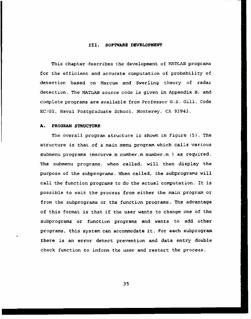
b. Swerling case 1 algorithm

Following equation is used to compute probability of

detection for case 1.

Po = - [ - -•(Y2 ]÷ 1 - ) - Yb -r•PDa=1 Y b (N 2 (l - ( ,N-2) e (1-Q

-Yb

=Pf,.(N- , ,y).(+5 (1- ~l pfa(N-_1,- Yb )e 1-1 N-i

Nrx 1+-1

(92)

It is obvious to see that for N=1 the detection probability is

e-lyb /'v,, The algorithm in computer independent notation which

uses equation (92) to compute PD is shown on Figure 19. Notice

in Figure 18 that the detection threshold (Yb) is independent

of the target fluctuation characteristics so that the

algorithm given in Figure 18 is used to determine Yb for all

target types. A MATLAB source code to compute probability of

detection of case 1 targets is given in Appendix B. The name

of this file is swerl!.m.

48

Enter Yb,N,X

XN - N* XY 4- Y

N 1

A 4- 0

DoH Y - EXP (-Y)

YMS4- YMM 0-N - M

N- I: H

YM .- YM Y/M

YMS - YMS + YMP, - YMS

A A

P1 4 P2

Y 4- .Y/(1 +1/Xw)

A, (1 +1/X,)"'l

A2 4- EXP (-Yb/(l + X.))

P3 4 Al * A2 o (1 -- P2 )P 4- P1 + P3 -- - - - - - - - - - -- > Exit Pot

- P 4-- EXP [ Yb (Xn + 1) 1--------- >Exit Pol

Figure 19: Algorithmic Program for 8werling I Target,Pol

c. Sww:rlij came 2 algorlthm

Eq(63) can be modified as:

49

(93)

pfa (N, (b

A computer independent algorithm to implement the above

equation is shown in Figure 20.

Enter Yb , N

X 4- (1+ N*X)

x0 4- Y/XYM 4- exp (-X 0o)

YMS4- YM

M 4- 0

4 4- M + 1

N M

y - X0*YM/M

YMS - YMS + YM

P0 2 4- XMS --------- > Exit Pd2

Figure 20: Algorithmic Program for Swerling 2 TargetP.,

50

d. Swerling care 3 algorithm

From Eq(75), the equation for probability of detection for

case 3 is as follows:

-Y (Nx)1.. (1- - y)

PD3 e 2 _2 _ for Nr 1(1+ Nx) 22

Y-- 2 e-Yb 2 Yb Nf÷2 N-2e -2r-N•+2+pf (N-1, Iyb) + (-e 2 (94)(N-2)1 N-2

(1- 2(N-2) + 2 ] [1-pts(N-1, Y±Nx)]; N>2NXV 9x--2 ffxt2

An algorithm for above equation is presented in computer

independent notation in Figure 21.

51

Enter Y,,N, X

y Y.-

N 1A 4- 0

YM E-fXP (-Y)

YMS YM

M 4- 0

M H l

rN-1 M

A - YM Y/H

"YM YM2 *- YHP2 Y..

P 4-- P2*" Y (1 #2/X.) __

4 .Al " i + 2/X")*"

A2 4" LXP (- 2Yb/(X(,+2))

A3 -- 1 - 2 (N-2)/(X4 * 2Y,/(X. , 2)

P3 4" Al A2 & A3 * (1 - P2)

2 N

L 4- N- 2

C L- L

L -- L -

0O L

S -- (C*L)

P4 - 2Yb"' o'b/Be (X,-2)

P 4-- 1* P2 + P3 ---------. Zxi Pp,

G .- .XP -2Yb/(I.2 )

H - Z XNG YT/(XN+2)'

P (- 0( N) ----------- -Exit P",

F1iguze 21t Algorithmic program for Swerling 3 Target, P,,

52

e. SwerlIng case 4 algorithm

Swerling case 4 computer prograr, modified expression can be

obtained by applying the power series in Eq (30) into Eq(81)

as

m - (1-P(N+k, 1+3/2 )H04' (+1/2) 2 k! (N-k)!

2M-1 + Nx NX- _( E[ e -2 1-- (95)

+ Ax mI O K! (N-K) 1

Y1 -- •' i+-LO

2 y2Y. NI -) K

n.ZN ml MK! (N-K)!]-(K(_ .

-i- 1•xN[f2W z-i' 1+2- • N, T-W) J+N -- 'V (N-L,W X-O)

Se)- 2 21+-L MI 71(NK

2

+(1+N-+X) e T 22 "2N ml

Y

2-"- NI ( X ,( • -m~e 2~ ___

M.0 m+

r2. __..•..) (-Nx NE e 2 NI 2+1

Lv )K( )X

men, mI x- K! (N-K) I 11.N2 /1+ INxN/2

Y Y

:-W,,-+aAIx/ 2 + emI

KI(N-K) 1 7.Nk12 14NxI2

53

with this expression the detection probability computation for

this case therefore can be simplified according to equation

(95) and avoid the computation of infinite power series. A

computer independent algorithm is at Figure 22.

Enter Yb,N, X

4 4-- X

M 4- 0

HK 4- ( 2 /(X. +2))NY •" Yb

B 4- 2Y/(X,. + 2)

YM e-

YMS -- YM

M 4- M +N M

4- YM * B/M

YMS- YMSS + YM

SUM YMSMKS 4- MK

YM - M B/Msum e SUM + YM (1-MKS)MK x- a. MK o (2N-M)/2(M-N+I)

,MKS e- MKS + MK

M +- M + 1

P4 - SUM ------- >EXit Pda

Figure 221 Algorithmic program Lor Smrling 4 Target, pV,

54

f. Swerling case 5 algorithm

In case 5, the expression of Marcum steady target model in

Eq (38) can also be modified by substituting the infinite

power series for the modified Bessel function IN(X) given by

(.2L) 2KIN(X ) 2 (96)

2( . K! (N+ K)!

and interchanging the order of summation and integration, one

obtain the probability detection for case 5 as:

PDS=e -IXo (NX)K N E K e-Y (97)A-0 K! m-0o M

By interchanging the order of the summation results in a

efficient computation representation as:

N-1 e b m ' - m' rný" -N t (V)98PD5 = %-Ž + e - (98)

m-0 K-0

The right hand side of equation (98) has two terms, the latter

term is a infinite summation of power series, therefore a

recursive evaluation is necessary for computing PD5 .

The method to handle this infinite power series is to

separate above equation into two terms. Let

PD5- PL + P4; (99)

where L represent the integrated pulses where L represent the

integrated pulses. Let L z N, then P•, can be represented as

55

N-1 m L m M-NP, -Yb y..• + e~y b• (1-K~ e-/ (NX)PL=•j e"b.•+~ &" m-.j K (100)

m-O * rn-N xa K!

the error term P, can be represented as

a ff In-N

P.= 1: e-Y--Y (1-E, e"-(Nx) (101)m-L*1 ! K0 K!

if let P, =ps then the truncated error term will be P.

P0- e- -Y ( - (Nx) ke -WT--O (102)

yK L. -NL:(z e -1, YK) Av l* ')

71- ki

Let L be large enough such that

e - k-L e TY "K L( -.1-N ((NX) ie - (103)

There fore

PD5 -PL,<e (104)

An upper bound can be found to limit the desired accuracy

and avoid the unnecessary computation. The computer

independent algorithm is in Figure 23.

56

enter" Yb.N,S

XN - X* N

YM -- _XP (-Yb)

YMS <-- YM

M -- 1N M-

YM <-- YH o Yb/M

YMS -- Y¶MS + YM

M - M +i

sUm - YMS

XB 4- EXP (-XN)

XES <- XB

YM 4- YM o Yb/M

YMS 4- YMS + YM

SUM <- SUM + YM (I - XBS)

M - M + 1

K - M - N

XB 4- XB o XN/K

XBS -- XBS + XB

5-< : (1 - YMS)(i - XBS)

P 4- SUM -------------- > eXIT WITH PDs

Figure 23: Algorithmic program for Swerling 5 Target, Pos

57

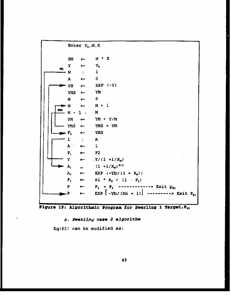
2. Solving for round off error

Round off error can take place during the calculation of

case 5. That is because during the calculation of probability

of detection, if the signal-to-noise ratio x is zero, the

output detection probability will become the probability of

false alarm, then the criterion in Eq (103) will become

-yK L-1-N (Nx)ke-Nx-Fe )1 k!M0 K! 0l

L-1-N (105)•(l-l) (1- •- (Nx)ke-x

•0

Since we can not set the minimum acceptable error to be

zero, the computation process will not terminate. Due to this

reason, trade-off between the accuracy and the maximum value

of output data should be made. An algorithm to compute the

threshold Yb to deal with the round off error is in Figure 24.

The corresponding MATLAB file name is Marcum.m which can be

used to compute the maximum acceptable threshold level Yb when

the value of signal-to-noise ratio is zero and the number of

pulses is large.

58

Enter Pfa,, O

Y

M 4- 0

YLX- 0

YLOG 4- LOG (Y)

TStJM 4- EXP (-Y)

M 4- M+1

M 4- N-1

SUNK( L OG(M)

'(LX 4- YLX+YLOG-SIJNK

TSTJM 4- TSUM+EXP ('LX-Y)

4- Y(4LOG (XPP&*TSUM) *TSUM/ EXP (YLX-.YIK £Y

Yb 4- Y - - - - - - ->Y

Y 4- ,

M 4- 0

'(LX 4- 0

'(LOG 4- LOG(Y)L Y-YLX: 1EM +-H1SUNK 4- LOG(N)'(LX 4- YLX*YLOG-SUNK

TUJM i- EXP(YLX-Y)

'(b Y, -- - -- - -- - - > .Y

Figure 24: Algorithmic Program for Detection Thresholds, Yb

with round off error preventation

59

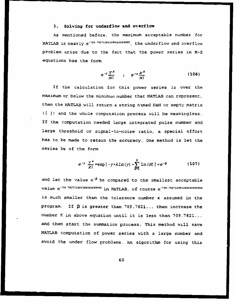
3. Solving for underflow and ovarflow

As mentioned before, the maximum acceptable number for

MATLAB is nearly e`° 9 "e19 3 4O 4 °9 9 99 99, the underflow and overflow

problem arise due to the fact that the power series in M-S

equations has the form

e- ; -e-x (106)

If the calculation for this power series is over the

maximum or below the minimui number that MATLAB can represent,

then the MATLAB will return a string nimed NaN or empty matrix

(C ]) and the whole computation process will be meaningless.

If the computation needed large integrated pulse number and

large threshold or signal-to-noise ratio, a special effort

has to be made to retain the accuracy. One method is let the

series be of the form

k• ke -Y X! =exp [ -ylkln (y) - ln (IV] =e-0 (107)

and let the value e- be compared to the smallest acceptable

value e"709.7271289338404099999) in MATLAB, of course e- 0 9 -70271289338&040999999

is mtch smaller than the tolerance number C assumed in the

program. If P is greater than 709.7821... then increase the

number K in above ecqu•ation until it is less than 709.7821...

and then start the summation process. This method will save

MATLAB computation of power series with a large number and

avoid the under flow problems. An algorithm for using this

60

method to compute the detection probability is in Figure (25),

and the MATLAB source code is thxeuhm.m and is given in

Appendix B.

a - -"I 0

a - a

LH - *xp(-tvi

IN OW V

a

E -AM YS.

fiMl - I +TrM

a N

IN In

(I M oil

u SU N

I N

N I - l IT Ni - TM-I

SVM - 'M Nl

MLA

14j .J . L.

Ar - 'i .US,,' - III•11

N2 I - NLT.LT.I J I

Tid11- TlMEllM'- 0

a - 1l a

'-- lxl - a

1* IRE (-ll *IIIf

*I l~iP -I -t l!

Pigaure 2S: Algorithmic porgraM for con~uting the probabilityof dtection,P.5 with underflow preventation

61

4. Input arguments and output data

The table below summarizes all input and output data for

the programs.

PROGRAM INPUT DATA OUTPUT DATA

THRESH.M PrA N yk

PROB.21 Yb,N Pr%

SWERLI .M Pf,, N, x PD1

SWERL2.M Pfa, N, X P02

SWERL3 .M Pf,, N, X PD3

SWERL4.M Pfa, N, X PD4

SWERL5.M Pf,,N, x PD5

THRESHM.M.m N, Pta Y1,

MARCUM.M Yb, N , x P., or Pf.

POINT.M N, x Pd (numerical)

RADPOINT.M N, x Pd (output data)

RADAR.M pfa,N, x CHART S/N vs Pd

RADAR1.M pf,,N, x CHART Pfa vs Pd

MEYER.M Pf,,N, X CHART N vs Pd

RANGE.1 pfa,N, x , HAPT R vs Pd

62

RANGE.3 ptAN , j.CHART R vs Pd .

Table 1 : Input arguments and output data

Where

N=Number of pulses to be integrated

R =average signal-to -noise ratio

Pd= probability of detection

pf,-probability of false alarm

R= the desired detection range

ns=Swerling case number

63

L~M

IV. RESULTS

The M-S detection probability curves can be obtain by

applying the I4TLAB programs in Chapter 3. The results can let

the user evaluate the detection probability detection

performance easily. The detection range curves can illustrate

relationship between the detection probability and the

detection range by input the properly detection loss.

A. PROBABILITY OF DETECTION CURVES

As menticned previously, the M-S model arise from the

different fluctuations of target cross section. MATLAB

programs can be used to plot probability of detection versus

per pulse signal-to-noise rat.I, for given probability of false

alarm for five cases. t -ý be asked to determine per

pulse signal-to-noise ratio "•wetired for given P0 and Pf.

This required signal-to-noise ratio can be used to compute

maximum detection range from the radar range equation.

Fig 26 and Fig 27 compare the five target models for a

false alarm of l0", and the number of integrated pulse as N=10

and N=100 respectively. When the probability is larger than

0.33, all four cases in which the target cross section is not

constant requires greater signal-to-noise ratio than the

constant cross section case. This increase in signal-to-noise-

ratio will cause a reduction in detection range. Therefore if

the characteristic of the target cross section are not

LM 64

properly take into account, the actual performance of the

radar might not measure up to the performance which is

predicted from the constant target cross section. A greater

signal-to-noise ratio is required when the fluctuations are

correlated pulse to pulse (case 1 and case 3 ) than when the

fluctuations are uncorrelated pulse to pulse(case 2 and case

4). Fig 27 also indicates that when the number of integrated

pulses is large, the case 2 and case 4 will approach to the

constant target case (case 5).

n = 109- Pfa =le06

€ 80-

70

0 60iUu- 50 1

t 404--

~30-

20

10

-5 0 5 10 15 20 25

(S/N)I, signal-to-noise ratio, DB

Figure 26: Probability of detection curves for five targetmodels

65

100

9o pfa l.o06 • -' -Ii

80h

70 ... 43

0 60r-Z 50•

'o 40

2010

0/5 0 5 10 15 20 25

Figure 27: Probability of detection curves for five targetmodels

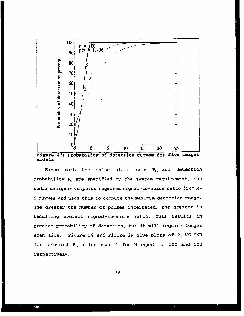
Since both the false alarm rate Pf. and detection

probability PD are specified by the system requirement, the

radar designer computes required signal-to-noise ratio from M-

S curves and uses this to compute the maximum detection range.

The greater the number of pulses integrated, the greater is

resulting overall signal-to-noise ratio. This results in

greater probability of detection, but it will require longer

scan time. Figure 28 and Figure 29 give plots of Pd VS SNR

for selected Pf.'s for case 1 for N equal to 100 and 500

respectively.

66

100 n - 100pfa - le-06 to le-12pfastep - 10

80" le-06X

M. 70o:S

c 60-

2 50 le-12

I, I

o3 40r-

S30-

2% 20 i-A. I

10010 -5 0 5 10 15 20

(S/N)I, signal-to-noise ratio, DB

Figure 28: Probability of detection curves for Swerling case

10 n- 500go pfa - le-06 to le-12

pfastep - 10

U le606F501

2. 67

Figure 30 and Figure 31 are the Swerling case 2 plots of

Pd Vs SNR with 10 and 100 pulses integrated respectively. From

Figure 30, signal-to-noise ratio of 4.8 db approximately is

required to yield a probability of detection of 0.8 with 10

pulses integrated and probability of false alarm of 10-6.

1001 n=10

90k pfa = le-06 to le-12pfastep = 10

~ 80 le-06&. 70

~650-

0~ 40- _• / 1€-12

303

2 20-

100o 2 4 6 8 10

(S/N)1, signal-to-noise ratio, DB

Figure 30: Probability of detection curves for Swerling case2

68

10n='100

9 pfa = I1-06 to lc-J2[pfastep = 10

80~ - le-06-80

S700

30 Ic /

u- /

•8 40k

8 20

10

01 .6 -4 -2 0 2

(5/N)I, signal-to-noisc ratio, DB

Figure 31: Probability of detection curves for Swerling case2

Figure 32 and Figure 33 show the Swerling case 3 with 10

and 100 pulses integrated respectively.

69

I n -- 10 11g0o. pfa a 1€-06 to le 4

i pfatep 10U 80,-.• , ~~~le.-Oi/;,/M 701-

c.2 602s~u 50, le-12

,Z 30'

0 20 1 /

0 5 10 15 20

(S/fl). Sgnal.io-noots ratio. DBFigure 32: Probability of detection curves for Swerling cast3

too. n- 100

-.. pfa - le.06 to lc. 1pfastep - 10 .,/o e* /1

SO.-Ie1

le.

260r

420- "t

30>1

10

o5 0 s 10 - 5

(S/N)I, sinl•-to-roase ratio, DB

Figure 33: Probability of detection curves for Swerling case3

70

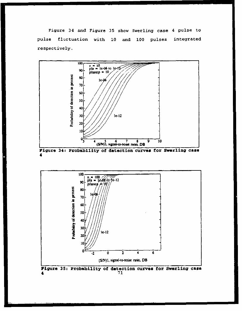
Figure 34 and Figure 35 show Swerling case 4 pulse to

pulse fluctuation with 10 and 100 pulses integrated

respectively.

100 n - 109o p(a - it-06 to I

pfwp- 7o .10I

80-

K7 0 -

S60-U /,//S50

100 40

S30 Ie*12

220-

10

3 4 5 6 7 8 9 1'0(S/N)i, sVWna.m-noise ratit DB

Figure 34: Probability of detection curves for Swerling case

t o o0 i n - 10 0 . ý :- / . M

So-), i~lo-oerai.D470

100

I SNI n-tOO.','s raio D

4K 70

S . ... . . . ...- " t ? • , , i a m , , |11. 9I 6

Figure 36 and Figure 37 are Swerling case 5 steady-state

target with 10 and 100 pulses integrated respectively.

100 n - 10r pf,- j 6 *A

90 1-

16 4 0 1i /,

75 30'!-,l

a_ /1'

16 0I. 1

50

3 4 5 6 7 S 9 10

(S/N)I, sipal-m-nom f tro. DB

Figure 36: Probability of detection curves for Swerling case4

100,.n . 10e06 to 1W•'pfastcp- a O '//0.90, Ph-/ e'

70' ep- /111w 80I Ii'!6

706 e.0

4'F.8 30 I l

2 20-

lO- ioi,,I I.4 .2 0 2 4

(SIN)! . si,, al- noise ratio, DR

Figure 37: Probability of detection curves for Swerling case4 72

B. THE DETECTIOON RANGE CURVES.

The ASR-9 radar is used as a sample to compute maximum

detection range. ASR-9 radar is designed for surveillance of

the terminal area around airports. A significant feature of

this S-band radar is its use of moving target detection (MTD)

processor which provides coherent integration among other

features. The parameters of the ASR-9 radar are given in table

below. Also tabulated is the empirically determined search

detection range on a 1 m2 target for the various Swerling

models with a PD =0.9 and Pf, =10'6.

ASR-9 PARAMETERS AND RANGE CALCULATION

P,-12oo kW ranges

f-2900 M~z Rk .39.41 nm,,1.0S us R2 =52.41 na

a "I RI"46.68 amGQ-33.5 db Rn57.29 nmG,-33.5 d& Rm-62.63 naNI-5 d4Lml2d]3O,1.3* LossesO"-750/secPRF"1200 pps Transmitter 2 d2BD-VP150 8z Receiver 2 dRPO,0.9 mismatch I dJlPt.-10" Integrator 1 dLp.al Collapsing I dB

Beam Shape 3 dBMTZ 2 d9

------------------- S- ------55

Total 12 4.3

Table 2 : ASR-9 PARAMETERS AMD RANGE CALCULATXOR

73

100 n = 3 s0 . . . ..90L- Pfa - le-06__

U 80- '"3¢ ,7

70'- i//// /(701-- 'i

~40r KS301-

Szoý

-s 0 1o is 20

(S/N)1. signal.to.noisc rauo, DB

Figure 38: Probability of detection curves for five targetmodels

n, -- •.

0.9 pfa - Ie-06\ \\,0.8k

0.7k \

*~0.6-0.5I

0.1

0 20 40 60 8o 100 120

DETECTION RANGE IN NAUTICAL MILES

Figure 39: Range detection curves

74

C- Numerical data outpuit from probability of detectioni

programu.

A table of values below is included for the purpose of

checking the programs.

N Y. case X.). 143271 X010 x.)1 82373 X.100 ___3__6.2178_

13.3155055 1 .0361 8109266 87 .2 84 80)S$70497 .6S4 7SS92794 524 374

2 .03619109261*7 .2143035170497 .4S475S92794S2 371557722127 IS71339S)749___________________4

3 .020271269SOSI .2912843t39447 *77944622707425 .9625961046032 .995941497060___________________S

4 0202659173723 .2916820913S96 . 7 7944704.34,n .9652S66475476 .995941410232

S 0O4%GS2017166 .2480481019045 .99722505333065 .999999SX92496 .999999519246

3 19.1291661 1 .1971701181235 .5149062S96313 .83647025963833 .9446918445347 .9121260632S&

2 .1630915130577 .7460903012970 .9792091144321S .999016946215'7 .195965068946

3 .1734365463374 .58699449Q)259 .945106SM5S289 .9933271492944 .99t23175354)

a

N Y case xv).102727 X-10 xw)1.62271 X6100 x-316.22 79

10 32.7013405 1 .4I5S434394S07 .7911151202531 .9232414527967 .9765960615308 .992S32970404

.73309703346765 *9 9 89 6 67 533i 9 3 .99999933532414 .9$99999999973 1

3 .5693747270410) .9139452695156 .980C436879910 .99380347197)1 .999077744289S

4 79173933715194 .999P6291g223s .99999$929999760 1 1 1

S 38355167194356 .99#99991524271 .999n"91524289 .99*9991524293 .' I9912620

N Y. Calla x-1-142276 W010 XS31.62278 re 100 xn316.2278

30 63.S481801 1 .69I526341e1006 .3917071.1566434 .96429073448000 .99G55331153) .99639654382053

2 .99944729942719 .99929999999999 1 1 1

3 .3147930711125 .9759019996594 .99723539213379

.99971901636700 .99997145717056l4 .999931272763193 1111

S .999 99674464$916 .9999992346033 .99999923440997 .99999928460997 .99999234460987

75

V. CONCLUSIONS AND RECOMMUNDATIONS

A. CONCLUSIONS

Radar detection theory is outlined in this thesis and

computer programs are developed for probability of detection

calculations in MATLAB. These programs are based on radar

detection theory as developed by Marcum and Swerling. These

programs give more accurate results than the commonly

available programs based on the detectability method which is

empirical is native. A user's guide and instruction are

included in the thesis. Simple examples of the programs usage

are illustrated in the thesis.

Students can use the programs written for this thesis to

investigate radar system performance. These programs are cost

effective, convenient to use and easy to reproduce since they

are run on personal computers that are readily available to

students. In particular, the program can aid students by

removing a major computational burden to allow him to perform

real world detection calculations. These programs can also be

used fjr calculations in radar development work.

B. RECOMMENDATIONS

Due to an overflow underflow problem the programs are

L

76

limited to integration of 600 pulses in the probability of

detection calculations for all 5 cases. Most of the time this

does not present any limitation as most radars integrate fewer

than 600 pulses. However it may be desirable to remove this

limitation by employing a Chernoff bound or other methods.

77

AVeondix A

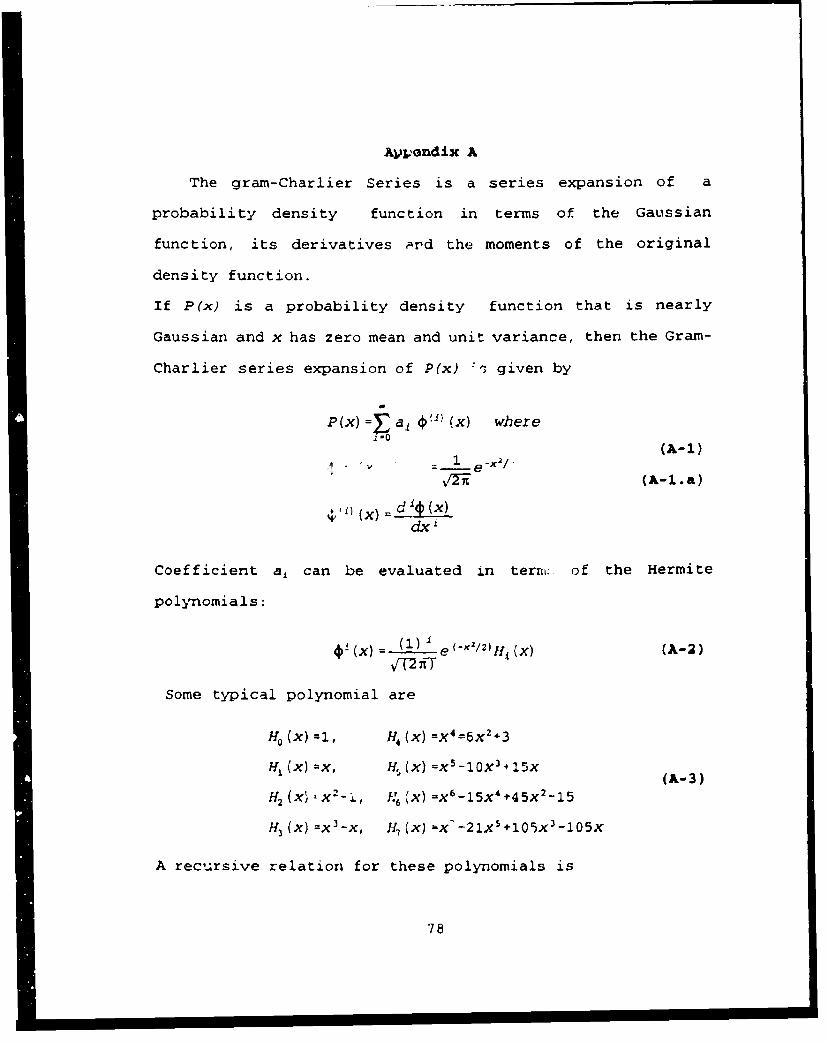
The gram-Charlier Series is a series expansion of a

probability density function in terms of the Gaussian

function, its derivatives ard the moments of the original

density function.

If P(x) is a probability density function that is nearly

Gaussian and x has zero mean and unit variance, then the Gram-

Charlier series expansion of P(x) 'i given by

P(x) =t a, $'1) (x) where

(A-i)

(A-1.a)•,i•~ 1x 0di (x)

dx'

Coefficient a, can be evaluated in term. of the Hermite

polynomials:

-f(W(T e(-x2/2)II (x) (A-2)

Some typical polynomial are

Iao (x) =1, H4 (x) =x 4 =6x 2'-3

H, (x) =x, H (x) =X'-1OX3 415X (A-3)H2 (XI . X2-i f;6 'X) -X6-15X4÷45X2-15

HI (X) =x3 -x, 1/.%(x)=x'-21x 5 +105x 3 -105X

A recursive relation for these polynomials is

78

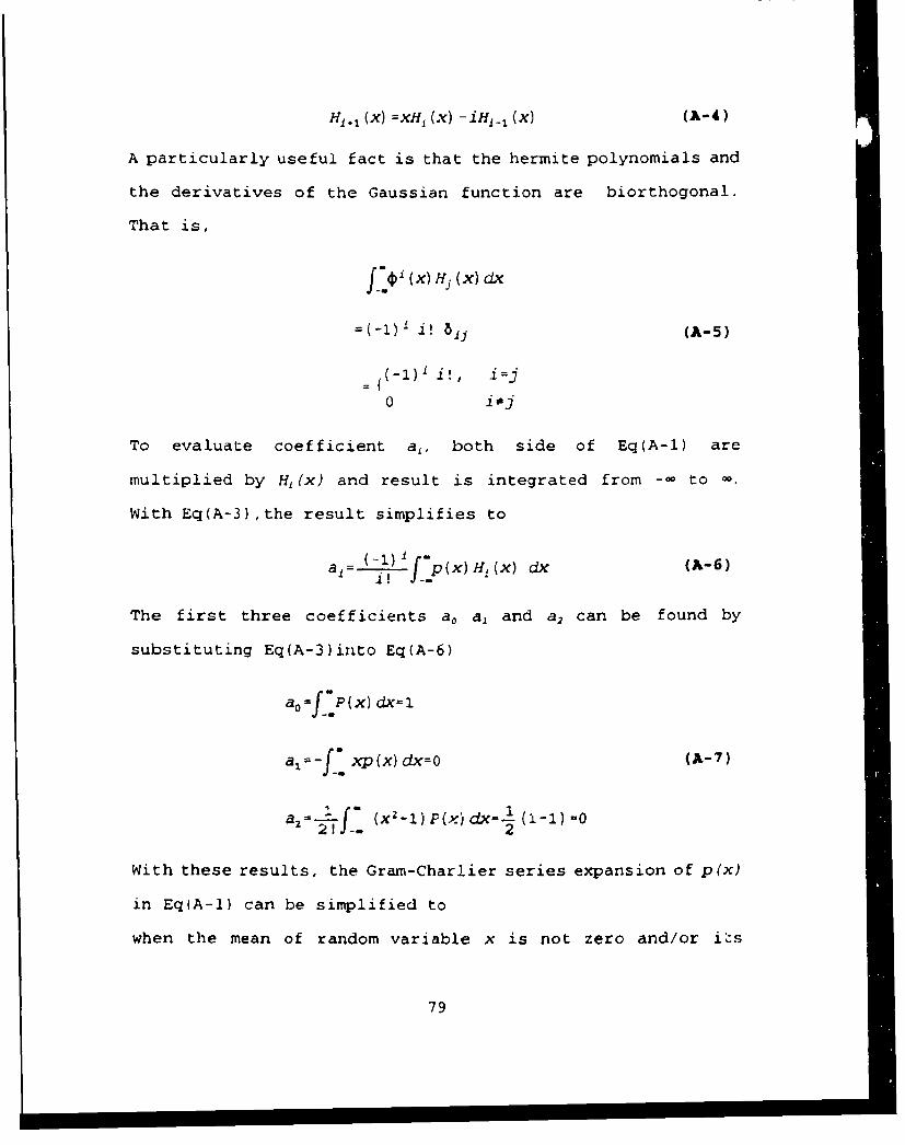
Hi., (X) =x•j (X) -in•-j (X) (A-4 )

A particularly useful fact is that the hermite polynomials and

the derivatives of the Gaussian function are biorthogonal.

That is,

f (x) Hj (x) dx

(A-5

0 i0j

To evaluate coefficient a,, both side of Eq(A-l) are

multiplied by H1 (x) and result is integrated from -- to •.

With Eq(A-3),the result simplifies to

a, =(x) Hi(x) dK (A-6)

The first three coefficients ao a, and a, can be found by

substituting Eq(A-3)into Eq(A-6)

a 0 LMP(x) dx=1

af xp(x) dx= (A-7)

a,= f" (x 2-l)P(x)dx- 2 (1-1)-021 2

With these results, the Gram-Charlier series expansion of p(x)

in Eq(A-1) can be simplified to

when the mean of random variable x is not zero and/or i's

79

p(x) 4 (x) +• €) (x) (A-8)

variance c is not unity, the Gram-Chazlier expansion of p(x)

is obtained by expanding a related density function g(t) in a

Gram-Charlier series, where

(A-9)

By a simple transformation of variables it follows that

p(x) g(t)

dx7t (A-10)

1 ,gx-___•o a

If the Gram-charlier series expansion for g(t) is

W

0~t = E• Cj4 W(i 0•' (A-11)

then from Eq(A-10) and Eq(A-ll), the expression for p(x)

becomes

P(x) Z-1r c,411x-__~ (A-12)}

If both sides of Eq(A-12) are multiplied by H,( (x- x ) 0 0]

and the result integrated from -- to -, coefficient ci can be

evaluated with relation (A-6) as

80

1 x dx (A-1 3)

Evaluating Eq(A-13) for the first few coefficients c, yields

co=l, C4 -= (c, ( -3

C5 1 CS--_10a 3 (A-.d)(5!)

C3 (6!) (a 6 -15a 4 +30)c 3 !- '' (6!)

where ok is the ith central moment of p(x), normalized by ce:

a•=-f. (x-x) 'p(x)dx (A-14)

The C4 can be expressed in terms of the conventional moments

of the distribution p(x); thus if n% denotes the nth moment

of p(x) that is

mn=Jxnp(x) dx (A-15)

then c; through % are related to noncentral moments min by

3_ m3 -3m 2m1 ÷2m12 4

m4 -4m~mj+6M2M2 -3m4

-~ ~ m15nm +Orm -1~~~+m~(-6 "4 a4(

m- -6mrm 1 +15m4m, -2 O 3mm +15xým4m -5mI

06

In summary, to obtain a Gram-Charlier series expansion,

the moments m, are found from Eq(A-16), or they can be

81

conveniently computed from the characteristic equation r-f the

distribution. Next the ai are evaluated using Eq(A-17) . The cXi

are then substituted into Eq(A-14) to obtain coefficient c1 of

Gram-Charlier expansion.

82

LMi

APPZWDX B

%FILE NAME: MS.Mclearclgclcecho on%THIS PROGRAM IS DESIGNED TO ALLOW THE STUDENT TO%VARY THE PARAMETERS OF THE VARIOUS SWERLING CASES%IN ORDER TO STUDY THE EFFECTS.% CASE #: DESCRIPTION% 1. Returned pulses are of a constant amplitude over one

scan, but are uncorrelated from scan to scan.% 2. Returned pulses are uncorrelated from pulse to pulse

and correlated from scan to scan.% 3. Returned pulses are of a constant amplitude over one

scan, but are uncorrelated from scan to scan.% 4. Returned pulses are uncorrelated from pulse to pulse

and correlated from scan to scan.% 5. The static case with constant S/N and pulse amplitudeecho offpauseclck=menu('MAIN MENU', 'THE H-S CURVES ',..'NUMERICAL DETECTION PROBABILITY CALCULATION',..'RANGE DETECTION CURVES'.)if k==lmscurveelseif k==2numberelseif k==3rmenuelseif k==4densityend% Now restart the process with some different choices% Clear the workspace of unnecessary data to avoidconflictsclear i; clear say; clear sdb; clear vv, clear pfa, clearp;clear ns;clear i; clear savy; clear sdbl; clear vv, clear pfal, clearp;% Check and see if any info is to changeclcecho on% If you want to restart the process ENTER CHOICE 1

or

83

% To exit this programPRESS RETURNecho offchoice = input('CHOICE =if choice==1

Mselseendclcecho on% You have chosen to exit the program

% Bye!echo off

% FILE NAME: RADAR.Mclc2ormat longecho

% THIS PROGRAM RETURNS THE PLOTS FOR THE NUMBER% OF PULSES AND SWERLING CASE SPECIFIED IN THE PARAMETERS.% THE PLOTS WILL BE STORED IN METAFILES UNDER THE NAME% "RADAR.MET" FOR AN EASY PRINT OUT.

% (A) the swerling case number has to be determined now

echo offns= input(-Enter the case number you want to study );

echo on

% (B). The number of radar pulses the program is to% integrate needs to be an integer between 1 and600.

echo offn-input( 'Number of Pulses to be integrated is nclCecho on

% (C). The probability of false alarm rate curves (pfa)to be plotted% must now be determined. Each choice of a pfa will resultin a different% curve being plotted on the graph. You need to choose thefollowing;

84

% 1. The smallest pfa curve to be plotted, pfamin = ?

% 2. The largest pfa curve to be plotted, pfamax =

% 3, The step size between pfamin aand pfamax, pfastep -

% If you wish to plot only one curve then enter the samevalue for

pfamin and pfamax.

The suggested default step size to use is that ofPFASTEP = 10,% which is quite sufficient. It is suggested thatpfamin and pfamax

be powers of 10 aL. that is the normal choice.

echo off

pfamin =input(,pfamin =pfamax -input(-pfamax =pfastep=input('pfastepclcecho on

% (D). The signal to noise ratio (S/N) in dB for whichyou wish to-

plot needs to be determined. The choices you needto. make are;

% 1. The smallest SIN point to be plotted, sdbmin ?

% 2. The largest S/N point to be plotted, sdbmax =?

% Remember that S/N must be entered in dB.

% 3. The stepsize between sdbmin and sdbmax =

echo offsdbmin =input('In dB the sdbmin is )sdbmax =input('In db the sdbmax is ')sdbstep= input('In db the sdbstep is )clgclCecho on%-------------------------------------------% CHECK YOUR PARAMETERS !

echo offfprintf('The case number you is %8 2f\n',ns);fprintf('The number of pulses yc¢ (noice are %8.2f\n',n);

85

fprintf('The max false alarm probability you choice is%8.2e\n',pfamax);fprintf('The min false alarm probability you choiceare%8.2e\n ,pfamin);fprintf(VThe pfa stepsize is %8.2f\nn,pfastep');fprintf('The max signal-to-noise ratio you choice is%8.2f\nr , sdbmax) ;fprintf('The min signal-to-noise ratio %8.2f\n',sdbmin);fprintf('The S/N stepsize is %8.2f\nl,sdbstep');echo on%--------------------------------------------%IF THE PARAMETERS ARE CORRECT PRESS 1%IF THE PARAMETERS ARE NOT CORRECT PRESS 2% ---------------------------------------------------

echo offchoice=input( CHOICE )if choice-=2radarelseif choice==lendecho on

% Now ryx. the calculations for the above data and plot it

echo off%delete radar.metformat longnmax = 700;axis ( 'square' );

r ci-•bmin sdbmax 0 100];axis (vv);if n < 2 I n > 600 1 n-=fix(n),

error('Number of pulses input exceeds dimensions')endif ns < . I ns > 5 I ns-=fix(ns),

error('Swerling case input does not correspond toallowable choices')end

pfa=pfamax;

sdb = sdbmin:sdbstep.sdbmax;kk=length(sdb);say = 10 ^(sdb/10);if ns == 1

swerlinglwhile pfa >= pfamin

for i= 1:kk%i = 1:sdbmax-sdbmin~lpW)=swerll(pfa,n,sav(i));

86

p(i)=l00*p(i);end

plot(sdb,p,'-);grid;title('SWERLING 1');xlabel( (S/Nfl., signal-to-noise ratio, DB'),ylabel('Probability of detection in percenttext(sdhmin +1/20*sdbmax,95 [,(n = I,int2str(n)])text(sdbmin +1/20*sdbxnax, 90,[(pfa=

,num2 str(p f amax) , 'to ' ,n=m2 str(p famin)]textisdbnuin +1/20*sdbmax, 85,[tpfastep

num2str (pf astep) I) ;gtext ( Enum2str (Pf a) I)hold onpfa = pfa/pfastep;

endpausemeta radar

elseif ns==2%swerling2p fa =p f amax;while pfa >= pfamin

for i= 2:kk% for i = 1:sdbmax-sdbm~in+lp(i) =swerl2 (pfa,n, sav(i) );p Wi=100 *piW

endplot(.sdb,p,'-'),title(ISWEP.LING 21);grid, xlabel( (S/Nmi. signal-to-noise ratio, DB'),ylabel('Probability of detection in percent')text(sdbmin + 1/20*sdbmax,95 Ptn I,int2str(n)])text(sdbmin +4 1/20*sdbma~x,90, t'pfa =~u~t~fmx,

to *,num2str(pfamin)])text(sd~bmin + l/20*sdbmax.85,Ppfastep=

,num2str (pf as tep) I1)gtext. ( tnum2str (pf a)])Ihold onpfa = pfa/pfastep;

endpause;meta radar

elseif ns==3%swerling3

if n == 1error('algori.thm for swerling 3 does not work for n1l')

endwhile pfa >= pfa~min

for i1l:kk%for i = 1;sdbmax-sdbmin4.Jp(i)=swerl3(pfa,n,sav(i));P(i)=l0O'p(i);

end

87

grid, xlabel( (S/Nfl., signal-to-noise ratio, OB'),ylabel('Probability of detection in percent,)text(sdbmiri + 1/20*sdbznax.95 Ptn =',int2str~n)])

text (sdbrnin + 1/2O*sdbrrax, 90, C pfa ='nun-L2str(pfamax) ,to ',num.2str(pfamin)])

text(sd~brin -t l.)20*sdbmax, 85, ['pfastep',num.2str(pfastep)))

gtext( fnum2str(pfa)]);hold onpfa = pfa/pfastep;

endpause;meta radar

e1seif ns==4%swerling4

while pf a >= pfaminfor i1l:kk

%fcr i = l:sdbniax-sd~bmin+lp(i)=swer14(pfa,n,sav(i));p(i)=100*p(i);

endplot(sdb,p,'-2;title('SWERLING 4');grid; xlabel('(S/N)l, signal-to-noise ratio, DB');ylabel('Probability of detection in percent')text(sd~bmin +ll2O*sdbmax,95 [Iln =',int2str(n)])

text(sd~bnin + 1/20*sdbmax.90'P~fa 1 ,num2str(pfamax),'to ',num2str(pfamin)1))

text(sdbmin + ll2O*sdbmax,85,(Ipfastep,num.2str(pfastepf)]

gtext( (num.2str(pf a)]hold onpfa = pfa/pfastep;

endpausemeta radar

else%swerling5

while pf a >= pfaminfor i1l:kk% for i = 1:sdbmax-sdbmin+lp(i)=swerl5(pfa,n,sav(i));P U) = 00*P (j)

endplot(sdb,p,'-'),title(SWERLING 5');grid, xlabel(' (S/N)l, signal-to-noise ratio, DE'),ylabel('Probability of detection in percent')text(sd~bmin + l/20*sdbmnax,95 [In = ,int2str(nf)]text(sd~bmin + 1/20*sdbmax,90,['pfa 1 ,num.2str(pfaznax),'

to ',nuxTL2str(ptamin) 1)text(sdbmin + l/20*sdbmax,85,flpfastep

88

' ,num2strlpfastep)])gtext( [num2str(pfa) );hold onpfa = pfa/pfastep;

endpausemeta radar

endhold off

%FILE NAME: SWERL1.Mfunction pd=swerll(pfa,n,sbar)

% RETURNS THE VALUE OF THE PROBABILITY OF DETECTION FOR THESWEPL•ING 1% CASE, GIVEN THE NUMBER OF PULSES n, THE PROBABILITY OFFALSE ALARM% PFA AND THE AVERAGE SIGNAL TO NOISE RATIO S/N.% EXAMPLE: SWERLl(PFA,N,SBAR);

format longyb=thresh(pfa,n);y=yb/(l+n*sbar);cteu (l+l/n/sbar);pd--prob (n-l, yb) ÷cte^ (n-l) *exp (-y) *( 1-prob (n-l, yb/cte )) ;returnend

% FILE NAME: SWERL2.M

% RETURNS THE VALUE OF THE PROBABILITY OF DETECTION FOR T1ESWERLING2% CASE, GIVEN THE NUMBER OF PULSES n, THE PROBABILITY OFFALSE ALARM% PFA AND THE AVERAGE SIGNAL TO NOISE RATIO S/N.% EXAMPLE: SWERL2(PFA,N,SBAR);

function pd=swerl2 (pfa, n, sbar)yb=thresh(pfa,n);y=yb/ (l+sbar)pd=prob(n,y);return

% FILE NAME: SWERL3.M

% RETURNS THE VALUE OF THE PROBABILITY OF DETECTION FOR THESWERLING3% CASE, GIVEN THE NUMER OF PULSES n, THE PROBABILITY OF

89

rAL"At A~1. V~A AMJ 714K AYLPA-N' ZIUfIKIL V) t1'I4ý1L P~ATIO -/Ui.

..XJj.L ...L .. .. .. . .. ...........

~ (tI-baa.obn-laytoI (nsba erp 1n~sat*) (I r-./I/LLy)

IU LUI Vt

PI PL IJAJ4K -vitiPL4 11

l0 V'JDftl~ '111L VAZAJ# (or 7h Q1Kar QF t.JKTKCTIQIJ ToI Tilt

% CA-wk, 0XzvijJ 'ri;t ttip-4jat wy PI."orKo i), INK1 IbADhIL2'rf OrrhLon AL.AIQ% nrA MIN TIMl hVYIMOV AIWJML TV 1lI9U P.ATIO 9/11.% PkAJP4Ai.K UWLP L4(IPr, 11, CAK) )%S@.wov *#eesg*@ too *.. ... 6 loti 4*oesre off 6* *oe 0 to 069C op efo 0#0

fUtivtkuf pedafwea44f I ~ ,a

i- ii (a, o )em~~i I~,

NUM 13 V1 I V,,

a~J11 * tiifli

I SiUL111

I Y'I1) 11I1til VAL'Th ur 7-1lt MIJtAPI'I 1 TY (Jr DLThCTIU1J PUR 77(1

3I~LJIJVU

% CASE, GIVEN THE NUMBER OF PULSES n, THE PROBABILITY OFFALSE ALARM% PFA AND THE AVERAGE SIGNAL TO NOISE RATIO S/N.% EXAMPLE: SWERL5(PFA,N,SBAR);

function pd-swerl5(pfan,sbar)ybuthresh(pfa,n);zanrsbar;YMcexp(-yb);OK = 0;kon;YMS-YM;for iul:k-1

YMuYM~yb/ i;YMS = YMS + YM;

endSUMSYMS;XBuexp(-z);XBSnXB;while OK x= 0

YMwYM*'yb/ k ;YMS = YMS + YM;SUMn 3UM÷ YM*(I-XBS);elal-YMS;XB =XB*z/(k-n1l);XBS a XBS + XB;e2ul-XBS;erael*e2;if er <- le-6OKwl;

endk * k + 1;

andpd a SUM;return;

% FILE NAME: THRESH.M

* RETURNS THE THRESHOLD yb FOR A GIVEN PROBABILITY OF FALSEALARM (pfa)

%I AND A GIVEN NMTBER OF PULSES%' EXAMPLE: THRESH(Pfa,N).

function yothresh(pfa,n)format longif n < 1 I n-ofix(n),

error('Wrong input number of pulses');break

endif numl

y--log(pfa);

91

returnendI =- loglO (pf a)n2=sqrt~n) ;l2sqrt(l);y=n-nf2+2.3*l2*(l2+fl2-l);,orrnpzle-6;ratio=J.;while comp <= ratio

p=prob(n,y);yin- ;

for k=l:1:fl-1;ym=ym/k~y;

end;ym~ym*exp(-y);delyz(p/ym)*log(p/pfa); % correction magitudey=y+dely;ratio=abs (dely/y);

endreturn

%FILE NAME: PROB.M

%*THIS PROGRAM RETURNS THE FALSE ALARM PROBABILITY P(n,yb)as in%* SIUhMhATORY(yb,^k/fact(k)) for k=O to n-1, AND IS A COMMflONFUNCTION

%*FOR THE PROBABILITY OF DETECTION COMPUTYATIONS

%* EAMPLE: PROB(N,YB)

function p=prob(x, y)if x< 0 1 X-=fix(x),error('Number of pulses should be integer and greater than

zero*) ,break, endinf==l .797693134862069'l0'^3Q8;E=709 .782712893384040999999;P=O;if x==0

return;elseif x==l

p = exp(-y);return;

else% .(if x>13

t=1;for k=l:l:x-1;-

t=t/k~y;P~t~p;

endp=(p41)*exp(-y);

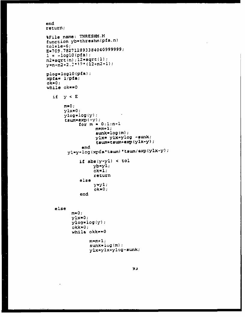
endreturn;

%File name; THRESH*14Mfunction ybothresh~fl(pf&al)tolmle-6;Eu709 .782712893384040999999;I2a -logIO(pf a)n2uscirt (n) ; 12usqrt (l)yzn-n2+2..'*I1I*(l2+n'-l);

plogologlO(pfa);xpfas 1/pfa;ok=0;while okan0

if y < E

ylxuO;ylogslogy);tsuznuexp(-y);

for m a O:2.:n-3.mum*1;sunkslog(m);ylxu ylx+y2.og -sunk;tslmmltsuI+OXP (ylx-y);

endy2..y~log(xpfcktsumI) *tsuw/GxpCylx-Y);

i.f abz(y-Yl) < tolyb-yl;

returnelse

yuyl;ok-O;

end

elsemaO;

yloguloeg(y);okk=Q;while okka-O

sunk-lug (i);ylxmylx~ylo.g-suflk;

if y-ylx <= E

tsumr=e.-p (ylx-y)okk=l;

elseokk=O;

endendif m >= n-i

yl=y~log(xpfa*tsum) * tsum/exp(-Y4-Ylx);if abs(yl-y) <~ tol

ybuyl;oku 1;break;return

elseyayl;okO0;

end

elsefor mr=m:l:n-1

sunk=log(m);ylx=ylx~ylog-sunk;tsuxn=tsum~exp (-y~y lx);

endyluy+log(xpfa*tsum)*tsumlexp(-y4-ylx);if abs(yl-y) <- tol

ybmyl;ok~l;break;return

elseycyl;ok=O;

endend

andend

%FILE 14AME: MARCLTM.Mfunction (p,ymojzbound(n,y,x)format longerr. le-6;Eft709 .78271289J3384040999999;

%****** start the program **~*********

lamdal- (n/ (2*y) )A+(n*x) /y;

auxlu(-lamda*y)*(n~x*laxnda) / (l-amda);

94

aux2=exp(au.xl)/I(1-laxnda) ý~n;if aux2 <= err

aux3=n*(x+l);if y >= aux3

p=O ;returnelse

p=l; returnend

else

ib~n-1;k0O;

if x <= Exk=exp(-x);xks=xk;m=O;

if y<= Eymn=exp (-y);yms~ym;

for m=l:n-lywI=ym*y/m;

if err>(l-yms)pUYM.S;YMO=ynMxrxln;

returnend

endrn=n-'L;swn=yms;

ok=O;while ok==O

k~k+l;m=m+l;Ymn=yn~y/m;ynm=y=sym;sumssum+ym (l-xks);xk~xk*xlk;xks=xks4-xk;ans=(l-yms) *(:--xks);

if ans<c= crrok~l;

endend

95

P=SUm;YMo-Ym';else

ymnly~O;yl.og~log(Y);okk=G;

while okk==Qrn=m+ 1;=f =log (M)

if (y-ynmly) <Eym~exp(-Y+YmlY);okk~l;

elseokk=O;

end

endi~f m <=ib

yms =yrn;

%-------------------------------------for tiL3=m:f-I

yrrvyrn*y/m;

I f err7('&-Yms)

ymozyT

ook~ml;enreturn

end

sum=yms;yrno~ymok=O;while ok==O;

k~k+l;

ym~ym*yIrfl

Y=s=Yms+ym;susuumtVy'm (1-xrs);xk~xk'x/k

xrs~xrs+xk;ans=(l-Ymfs)*(l-xrs);

if ans >erreeok=O;

break;return;

ok=1;eiid

endp=sum; ymo~ym;

else-------------------for mr'> ib;yino=O;returnyns =ym;suznQ;kd=m-n;if kd> x

p=O;x=x/n;break;return;

elseokkk=O;while okkk-.-O;

k=k~l;kk=xk~x/k;xks~xks+xk;

while (k-kd) < 0okkkQO;

endendooook=O;while ooook==0;

sum=sum+ym* (l-xrs);xk~xkx/k;x~rs=xrs~xk;ans=(l-yrns) *(l-xrs);while ans < err

p= sum;xx/f;ooook=l;break;return

endk=k+l;m=mn~l;yflp~ymf*y/m;yms=YMS+Ym;ooook=0;

end

endend

end

elsexklx=O;

97

x3.og=log(x);ooookQ:;whi.le oookO=

xklx==xklx+xlog-xkf;

oook=O;end

endxk~exp(-x+xklx);ib~ib~k;

xks=xk;M=O;

if y<= Eym~excp(-y);yms =ym;

for m=l:n-lym=ymn*y/rn;yms=ymS+ym;

if err>(l-yms)pyrrns;ymO~yrn;

returnend

endSUmflyrml;YMO =ynM;ok=O;while ok==O;

k~k+l;m=tn+l;ym=ym*y/m;Yrr=YMsyrsym;sum=sum+ym* (1-xrs);xk=xk*x/ k;xrs=xrs~xk;ans=(l-yms) *(l-xrs);

if ans<= errok~l;

endendp =sum;

elseymly=Q;ylog=iog(y);okk=O;while okk==O

98

m=rrl4;,xnf=log(m);

if (y-ymly) <= Eym~exp(-y+yrfly);okk=l;

elseokk=O;

endendif m <= ib.yns~ym;

---------------------------------------ook=O;while oo'==O

while m-'=2bm=m+l;ym~ym*y/m;ymm=ynm~syrf;if err>(l-ymTs)

ymo=ym;x-x/fl;ook~l;break;return

elseook=O;

endend

endsuxrlyms;yrmo=ym;ok=Q;while ok==O;

ym=yffly/;yms=yms*y/m;suxn=sum+ym* (l-xrs);xk~xk*x/k;

xrs~xrs+xk;ans=(l-ymns)*(l-xrs);

if ans > errok=O;

elsep= sum;x=x/n;break;return;

99

ok~l;end

end

else % ------ for m> b

ymsym";sum- 0 ,kd=m-n;if kd>x

P=Q;x=x/fl;break;return;

elseokkk0,while okkk==0;

k=k~l;ik~xk~x/ k;xks~xks~xk;

while (k-kd) < 0ok)ck-0,

end end

ooook0O;while ooook0=;

suznSUM+YM*(l-xrs);xk~xk*x/k;xrs~xrs~xk;ans=(l-yms)*(l-xrs);while ans < err

p =sum;x=x/fl;ooook~l;break;return

endk=k+l;m=m+l;ym~yImly/mf;y~s =yms +ym;ooook-O;

end

endend

end

endend

100

LIST OF REFERENCES

1. J. Marcum, "A Statistical Theory of Target Detection byPulsed Radar," Institute of Radio Engineer Transations ninformation theory., Vol. IT-6, No. 2, April 1960

2. J. Marcum, "A Statistical Theory of Target Detection byPulsed Radar Mathematical Appendix," Institute of RadioEngineer Transations on information theory., Vol. rT-6,No. 2, April 1960

3. P. Swerling, "Probability of Detection for FluctuatingTargets," Institute of Radio Enginee-?r Transations oninformation theory., Vol. IT-6, No. 2, April 1960

4. D. Meyer and H. Meyer, Radar Target Detection Handbook ofTheory and Practice, Academic Press, New York, 1973.

5. G. A. Campbell and R. M. Foster, Fourier integrals forPractical Applications., Van Nostr and Reinhold,Princeton, New Jersey, 1947 ; Bell Telephone Syst.Monograph No. B-584

6. Lamont V. Blake, Radar Range Performance Analysis, D. CHeath and company Lexington, MA, 1980

7. Anthony D. Whalen, Detection of Signal in Noise, AcademicPress, Inc. New York, 1971

8. M.I Skolnik, Introduction to Radar System, McGrow-Hill,NewYork, 1980

9. J. DiFranco and W. Rubin, Radar Detection, Arthech House,Dedham, MA, 1968

10. D. Curtis Schleher, Introduction to Electronic Warfare,Artech House Inc, 1986

11. The Math Works Inc, The Student edition of MATLAB,Prentice-Hall, Inc. A Simen & Schuster Company EnglewoodCliffs, New Jerrey. 1992.

101

INITIAL DISTRIBUTION LIST

No. Copies1. Defense Technical Information Center 2

Cameron StationAlexandria VA 22304-6145

2. Library, Code 052 2Naval Postgraduate SchoolMonterey CA 93943--5002

3. Chairman, Code EC 1Department of Electrical and Computer EngineeringNaval Postgurate SchoolMonterey, CA 93943-5121

4. Professor G.S. Gill, Code EC/GI 2Department of Electrical and Computer EngineeringNaval Postgurate SchoolMonterey, CA 93943-5121

5. Professor R. Janaswamy, Code EC/JsDepartment of Electrical and Computer Engineering 1Naval !-ostgurate SchoolMonterey, CA 93943-5121

6. Naval Academy Library 2Kao-Hsiung Tso-Ying P.O BOX 90175Taiwan, R.O.C.

7. -hung Cheng Institute of Technology 1Taoyuan, Taiwan, R.O.C.

8. War Game Armed Forces 2University Republic of China P.O BOX 90040-16Daje Taipei Taiwan

102