S. BoydEE102 Lecture 1 Signals notation and meaning common signals size of a signal qualitative...
26
S. Boyd EE102 Lecture 1 Signals • notation and meaning • common signals • size of a signal • qualitative properties of signals • impulsive signals 1-1
-
Upload
eustacia-sims -
Category
Documents
-
view
227 -
download
0
Transcript of S. BoydEE102 Lecture 1 Signals notation and meaning common signals size of a signal qualitative...
S. Boyd EE102
Lecture 1Signals
• notation and meaning
• common signals
• size of a signal
• qualitative properties of signals
• impulsive signals
1-1

Signals
a signal is a function of time, e.g.,
• f istheforceonsomemass
• vout is the output voltage of some circuit
• pistheacousticpressure atsomepoint
notation:
• f,vout,porf(·),vout(·),p(·)refertothewholesignal orfunction
• f(t),vout(1.2),p(t+2)refertothevalue ofthesignalsattimest,1.2,and t + 2, respectively
for times we usually use symbols like t, τ , t1, . . .
Signals 1-2

Example
1
0
−1−1 0 1 2 3
t (msec)
Signals 1-3
Domain of a signal
domain of a signal: t’s for which it is defined
some common domains:
• all t, i.e., R
• nonnegative t: t ≥ 0(here t = 0 just means some starting time of interest)
• tinsomeinterval: a≤t≤b
• tatuniformlysampledpoints: t=kh+t0,k=0,±1,±2,...
• discrete-time signals are defined for integer t, i.e., t = 0, ±1, ±2, . . .(here t means sample time or epoch, not real time in seconds)
we’ll usually study signals defined on all reals, or for nonnegative reals
Signals 1-4

Dimension & units of a signal
dimension or type of a signal u, e.g.,
• real-valued or scalar signal : u(t) is a real number (scalar)
• vector signal : u(t) is a vector of some dimension
• binary signal : u(t) is either 0 or 1
we’ll usually encounter scalar signals
example: a vector-valued signal
v1v= v2
v3
might give the voltage at three places on an antenna
physical units of a signal, e.g., V, mA, m/sec
sometimes the physical units are 1 (i.e., unitless) or unspecified
Signals 1-5
Common signals with names
• aconstant(orstaticorDC)signal: u(t)=a,whereaissomeconstant
• the unit step signal (sometimes denoted 1(t) or U (t)),
u(t) = 0 for t < 0, u(t) = 1 for t ≥ 0
• the unit ramp signal,
u(t) = 0 for t < 0, u(t) = t for t ≥ 0
• arectangular pulse signal,
u(t) = 1 for a ≤ t ≤ b, u(t) = 0 otherwise
• asinusoidal signal:u(t) = a cos(ωt + φ)
a, b, ω, φ are called signal parameters
Signals 1-6
Real signals
most real signals, e.g.,
• AM radio signal
• FM radio signal
• cable TV signal
• audio signal
• NTSC video signal
• 10BT ethernet signal
• telephone signal
aren’t given by mathematical formulas, but they do have definingcharacteristics
Signals 1-7

Measuring the size of a signal
size of a signal u is measured in many ways
for example, if u(t) is defined for t ≥ 0:
∫ ∞• integral square (or total energy ): u(t)2 dt
0
• squareroot of total energy∫ ∞
• integral-absolute value: |u(t)| dt0
• peak or maximum absolute value of a signal: maxt≥0|u(t)|( )1/2∫ T
• root-mean-square (RMS) value:
• average-absolute (AA) value: lim
1lim u(t) 2 dt
T →∞T 0
∫ T1|u(t)| dt
T →∞ T 0
for some signals these measures can be infinite, or undefined
Signals 1-8

example: for a sinusoid u(t) = a cos(ωt + φ) for t ≥ 0
• the peak is |a|
√• the RMS value is |a|/ 2≈0.707|a|
• the AA value is |a|2/π ≈ 0.636|a|
• the integral square and integral absolute values are ∞
the deviation between two signals u and v can be found as the size of thedifference, e.g., RMS(u − v)
Signals 1-9

Qualitative properties of signals
• udecays ifu(t)→0ast→∞
• uconverges ifu(t)→aast→∞(aissomeconstant)
• uisbounded ifitspeakisfinite
• uisunbounded orblowsup ifitspeakisinfinite
• uisperiodic ifforsomeT >0,u(t+T)=u(t)holdsforallt
in practice we are interested in more specific quantitative questions, e.g.,
• how fast does u decay or converge?
• how large is the peak of u?
Signals 1-10
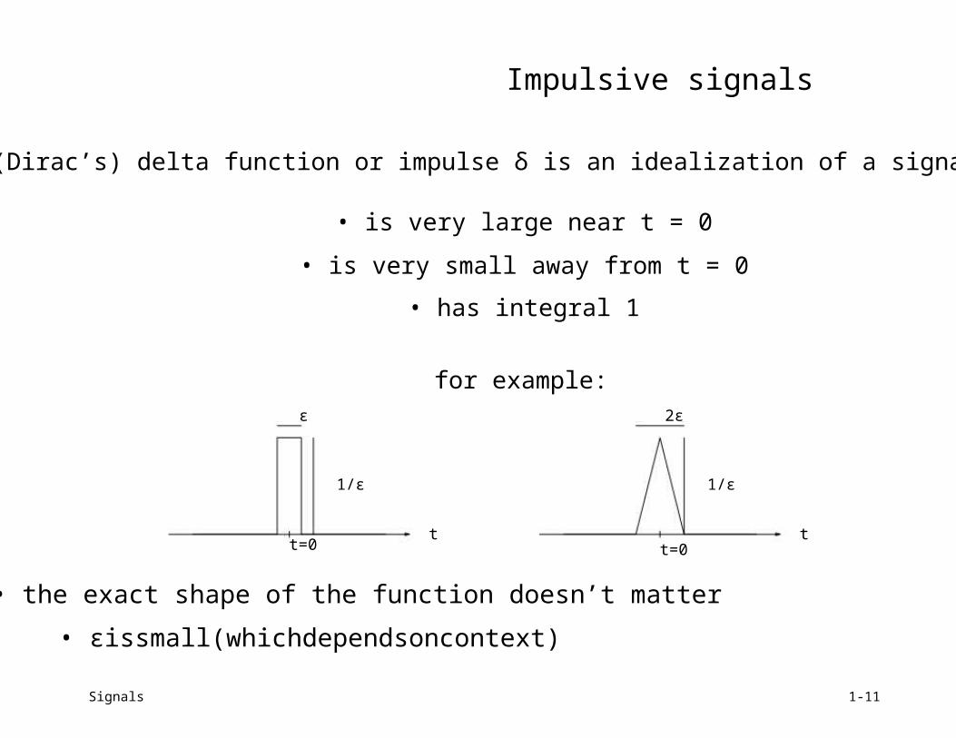
Impulsive signals
(Dirac’s) delta function or impulse δ is an idealization of a signal that
• is very large near t = 0
• is very small away from t = 0
• has integral 1
for example:ϵ 2ϵ
1/ϵ 1/ϵ
t tt=0 t=0
• the exact shape of the function doesn’t matter
• ϵissmall(whichdependsoncontext)
Signals 1-11
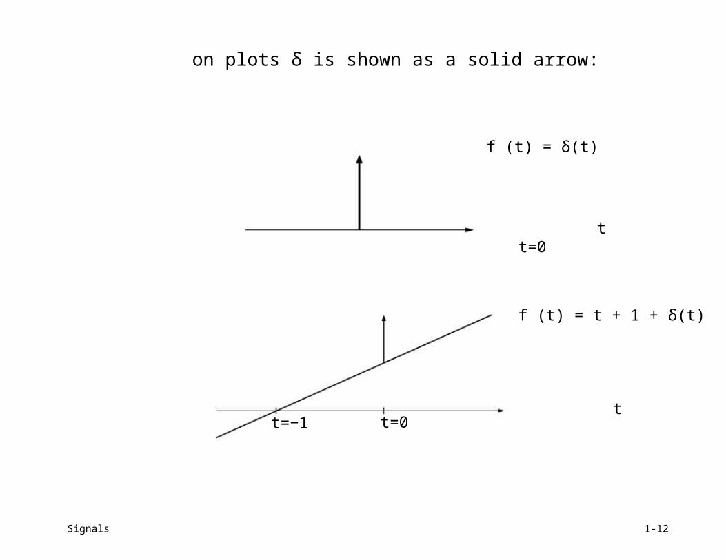
on plots δ is shown as a solid arrow:
f (t) = δ(t)
tt=0
f (t) = t + 1 + δ(t)
tt=−1 t=0
Signals 1-12

Formal properties
formally we define δ by the property that
∫ bf (t)δ(t) dt = f (0)
a
provided a < 0, b > 0, and f is continuous at t = 0
idea: δ acts over a time interval very small, over which f (t) ≈ f (0)
• δ(t) = 0 for t = 0
• δ(0) isn’t really defined
∫ b• δ(t) dt = 1 if a < 0 and b > 0
a
∫ b• δ(t) dt = 0 if a > 0 or b < 0
a
Signals 1-13

∫ bδ(t) dt = 0 is ambiguous if a = 0 or b = 0
a
our convention: to avoid confusion we use limits such as a− or b+ todenote whether we include the impulse or not
for example,
∫ 1 ∫ 1 ∫ 0− ∫ 0+
δ(t) dt = 0, δ(t) dt = 1, δ(t) dt = 0, δ(t) dt = 10+ 0− −1 −1
Signals 1-14

Scaled impulses
αδ(t − T) is sometimes called an impulse at time T, with magnitude α
we have∫ b
αδ(t − T)f(t) dt = αf(T)a
provided a < T < b and f is continuous at T
on plots: write magnitude next to the arrow, e.g., for 2δ,
2
0
Signals
t
1-15
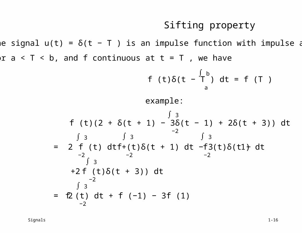
Sifting property
the signal u(t) = δ(t − T ) is an impulse function with impulse at t = T
for a < T < b, and f continuous at t = T , we have
∫ bf (t)δ(t − T ) dt = f (T )
a
example:
∫ 3
f (t)(2 + δ(t + 1) − 3δ(t − 1) + 2δ(t + 3)) dt−2
∫ 3 ∫ 3 ∫ 3
= 2 f (t) dt + f (t)δ(t + 1) dt − 3 f (t)δ(t −1) dt−2 −2 −2
∫ 3
+2 f (t)δ(t + 3)) dt−2
∫ 3
= 2 f (t) dt + f (−1) − 3f (1)−2
Signals 1-16
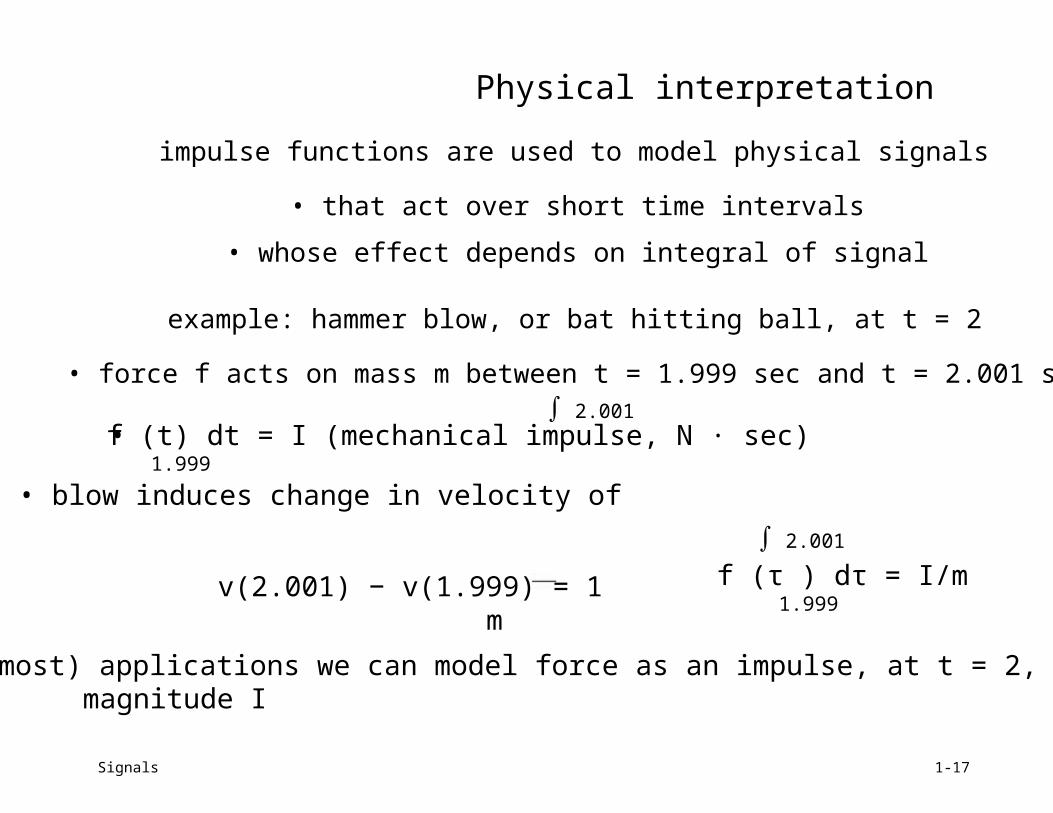
Physical interpretation
impulse functions are used to model physical signals
• that act over short time intervals
• whose effect depends on integral of signal
example: hammer blow, or bat hitting ball, at t = 2
• force f acts on mass m between t = 1.999 sec and t = 2.001 sec∫ 2.001
• f (t) dt = I (mechanical impulse, N · sec)1.999
• blow induces change in velocity of
v(2.001) − v(1.999) = 1m
∫ 2.001
f (τ ) dτ = I/m1.999
for (most) applications we can model force as an impulse, at t = 2, withmagnitude I
Signals 1-17
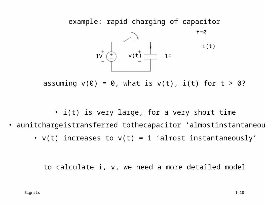
example: rapid charging of capacitor
t=0
i(t)
1V v(t) 1F
assuming v(0) = 0, what is v(t), i(t) for t > 0?
• i(t) is very large, for a very short time
• aunitchargeistransferred tothecapacitor ‘almostinstantaneously’
• v(t) increases to v(t) = 1 ‘almost instantaneously’
to calculate i, v, we need a more detailed model
Signals 1-18

for example, include small resistanceR
i(t)
1V
i(t) = dv(t)dt
1
v(t) = 1 − e−t/R
R
v(t)
= 1−v(t), v(0) = 0R
1/R
i(t) = e−t/R/R
R
as R → 0, i approaches an impulse, v approaches a unit step
Signals 1-19

as another example, assume the current delivered by the source is limited:if v(t) < 1, the source acts as a current source i(t) = Imax
i(t)
v(t)
Imax v(t)
i(t) = dv(t)= Imax, v(0) = 0dt
i(t)1 Imax
1/Imax 1/Imax
as Imax → ∞, i approaches an impulse, v approaches a unit step
Signals 1-20
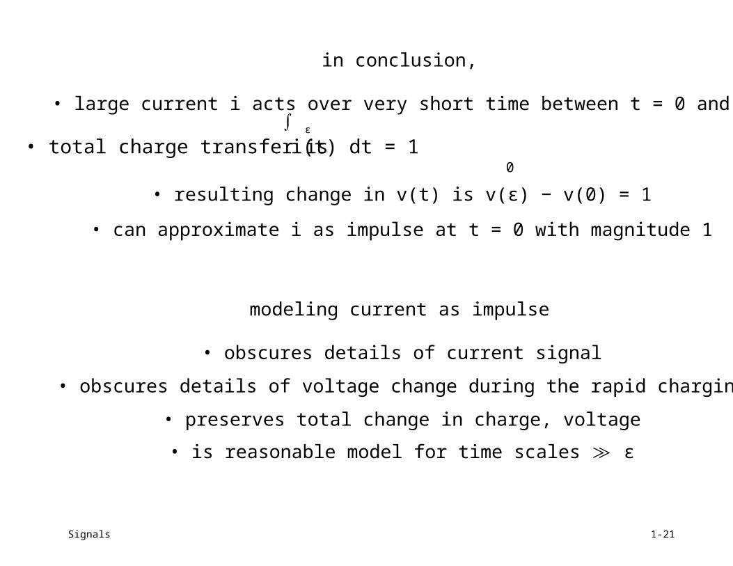
in conclusion,
• large current i acts over very short time between t = 0 and ϵ∫ ϵ
• total charge transfer is i(t) dt = 10
• resulting change in v(t) is v(ϵ) − v(0) = 1
• can approximate i as impulse at t = 0 with magnitude 1
modeling current as impulse
• obscures details of current signal
• obscures details of voltage change during the rapid charging
• preserves total change in charge, voltage
• is reasonable model for time scales ≫ ϵ
Signals 1-21

Integrals of impulsive functions
integral of a function with impulses has jump at each impulse, equal to themagnitude of impulse
∫ t
example: u(t) = 1 + δ(t − 1) − 2δ(t − 2); define f (t) =u(τ ) dτ0
1
u(t)
tt=1 t=2
2
f (t) = t for 0 ≤ t < 1, f (t) = t+1 for 1 < t < 2, f (t) = t−1 for t > 2
(f (1) and f (2) are undefined)
Signals 1-22
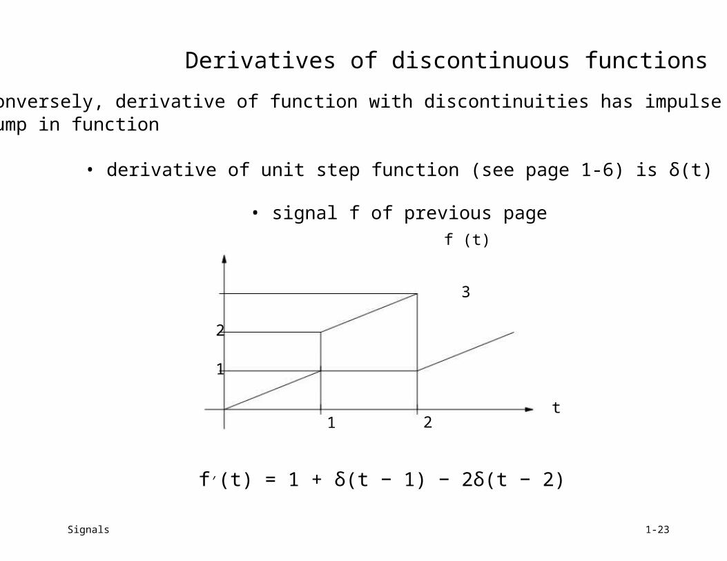
Derivatives of discontinuous functions
conversely, derivative of function with discontinuities has impulse at eachjump in function
• derivative of unit step function (see page 1-6) is δ(t)
• signal f of previous pagef (t)
3
2
1
t1 2
f′(t) = 1 + δ(t − 1) − 2δ(t − 2)
Signals 1-23
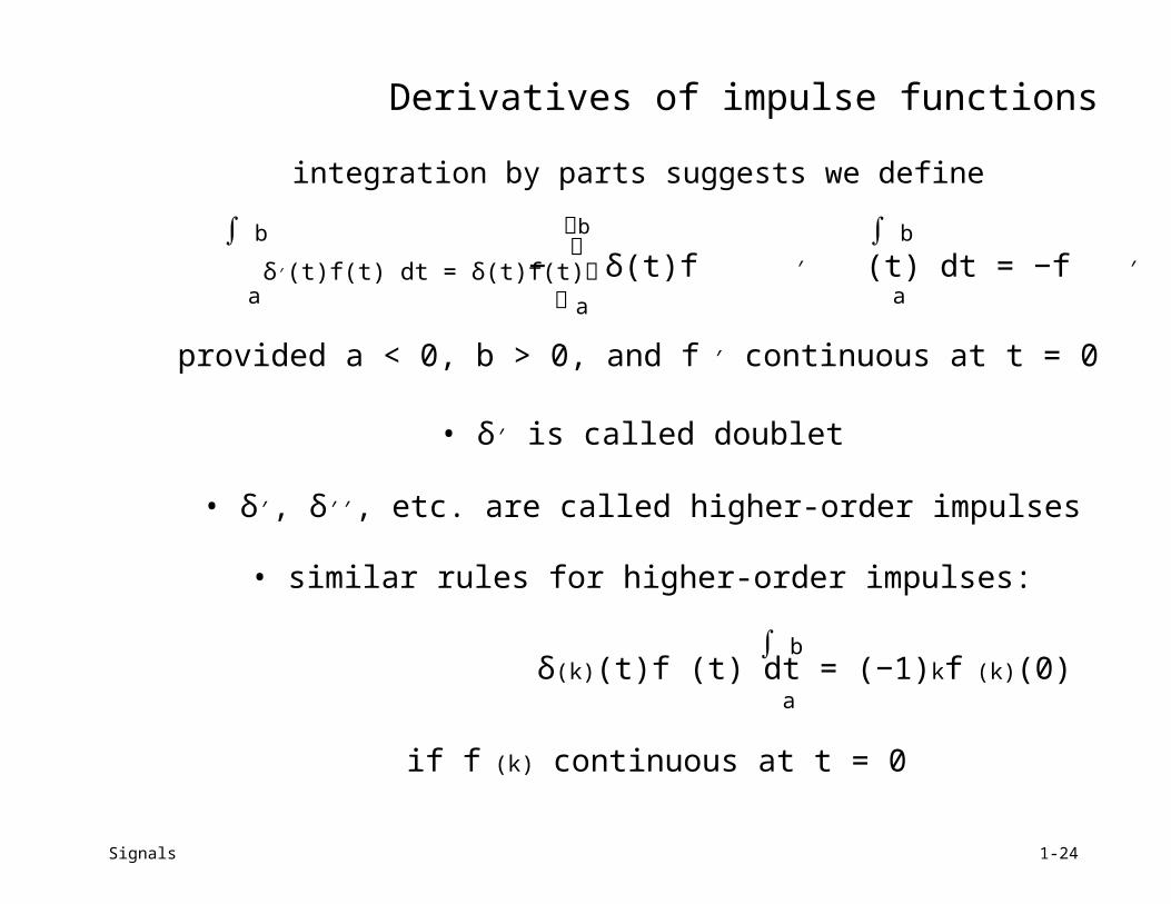
Derivatives of impulse functions
integration by parts suggests we define
∫ b
a
b
δ′(t)f(t) dt = δ(t)f(t)a
∫ b
− δ(t)f ′ (t) dt = −f ′ (0)a
provided a < 0, b > 0, and f ′ continuous at t = 0
• δ′ is called doublet
• δ′, δ′′, etc. are called higher-order impulses
• similar rules for higher-order impulses:
∫ bδ(k)(t)f (t) dt = (−1)kf (k)(0)
a
if f (k) continuous at t = 0
Signals 1-24
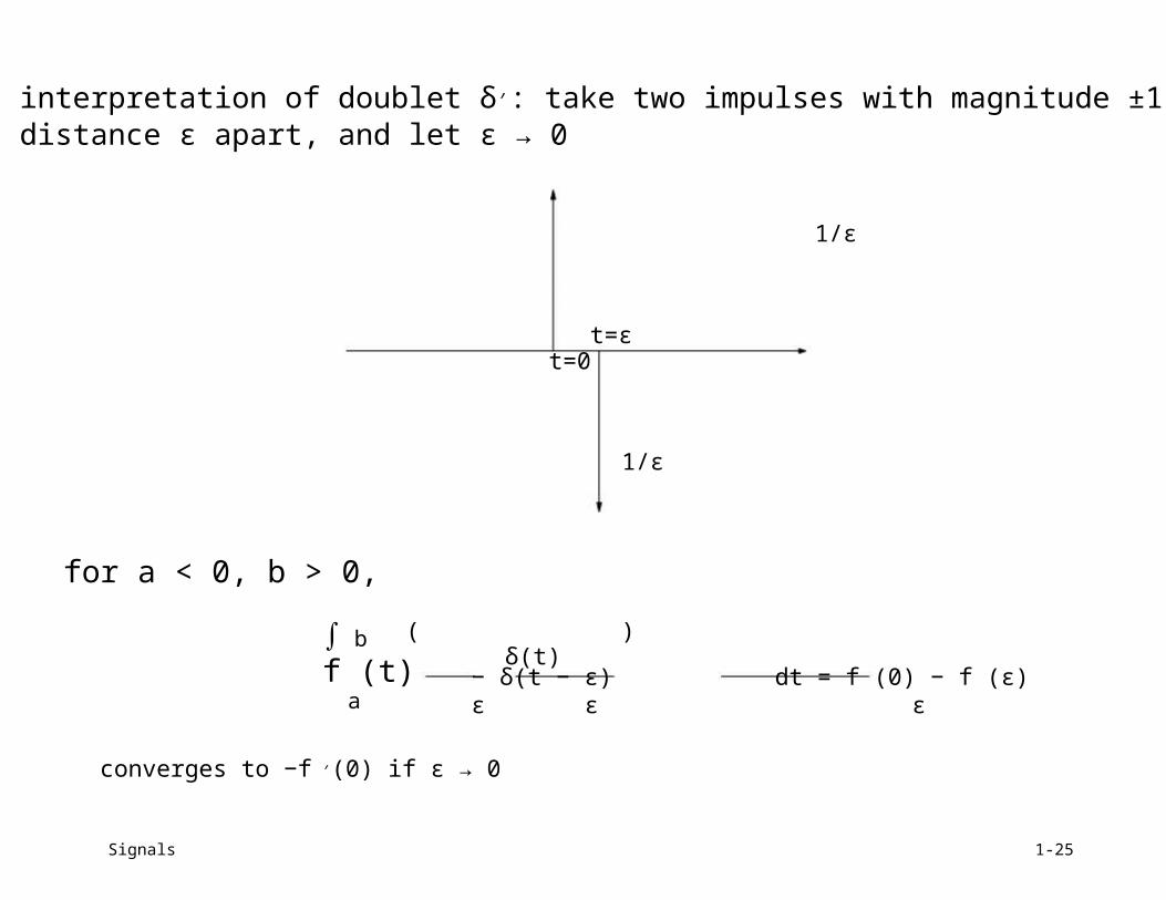
interpretation of doublet δ′: take two impulses with magnitude ±1/ϵ, adistance ϵ apart, and let ϵ → 0
1/ϵ
t=ϵt=0
1/ϵ
for a < 0, b > 0,
∫ b
f (t)a
( )δ(t)
− δ(t − ϵ)ϵ ϵ
dt = f (0) − f (ϵ)ϵ
converges to −f ′(0) if ϵ → 0
Signals 1-25
Caveat
there is in fact no such function (Dirac’s δ is what is called a distribution)
• we manipulate impulsive functions as if they were real functions, whichthey aren ’ t
• it is safe to use impulsive functions in expressions like
∫ b ∫ b
f (t)δ(t − T ) dt, f (t)δ′(t − T ) dta a
provided f (resp, f ′) is continuous at t = T , and a = T , b = T
• some innocent looking expressions don’t make any sense at all (e.g.,δ(t)2 or δ(t2))
Signals 1-26


![6.003: Signals and Systemsweb.eng.fiu.edu/andrian/EEL3135/convolution.pdfConvolution operates on signals not samples. Unambiguous notation: ∞ x[k]h[n − k] ≡ (x ∗ h)[n] k=−∞](https://static.fdocuments.in/doc/165x107/5f40eed83ac68f73fc179f03/6003-signals-and-convolution-operates-on-signals-not-samples-unambiguous-notation.jpg)