THE STUDY OF TWO-PARTICLE RESPONSEFUNCTIONS IN STRONGLY CORRELATED

ELECTRON SYSTEMS WITHIN THE DYNAMICALMEAN FIELD THEORY

BY HYOWON PARK

A dissertation submitted to the

Graduate School—New Brunswick

Rutgers, The State University of New Jersey

in partial fulfillment of the requirements

for the degree of

Doctor of Philosophy

Graduate Program in Physics and Astronomy

Written under the direction of

Prof. Kristjan Haule

and approved by

New Brunswick, New Jersey

October, 2011

ABSTRACT OF THE DISSERTATION

The study of two-particle response functions in strongly

correlated electron systems within the dynamical mean

field theory

by Hyowon Park

Dissertation Director: Prof. Kristjan Haule

In this thesis, we tackle various problems in strongly correlated electron systems, which can be

addressed properly via the non-perturbative dynamical mean field theory (DMFT) approach

using the continuous time quantum Monte Carlo method as an impurity solver. First, we

revisit the old Nagaoka ferromagnetism problem in the U = ∞ Hubbard model and study the

stability of the ferromagnetic state as a function of the temperature, the doping level, and the

next-nearest-neighbor hopping t′. We then address the nature of the Mott transition in the two-

dimensional Hubbard model at half-filling using cluster DMFT. Cluster DMFT can incorporate

the short-range correlations beyond DMFT by extending the spatial range in which correlations

are treated exactly to a finite cluster size. The non-local correlations reduce substantially the

critical interaction U and modify the shape of the transition lines in the phase diagram.

We then concentrate on the calculation of two-particle response functions from the ab initio

perspective by means of computing the one-particle excitation spectrum using the combination

of the density functional theory (DFT) and DMFT and extracting the two-particle irreducible

ii

vertex function from a local two-particle Green’s function computed within DMFT. In particu-

lar, we derive the equations for calculating the magnetic/charge susceptibility and the pairing

susceptibility in superconductivity. This approach is applied to the Hubbard model and the

periodic Anderson model and we determine the phase diagram of magnetism and supercon-

ductivity in these models. We show that the superconducting phase is indeed stable near the

magnetic phase where the pairing interaction mediated by spin fluctuations is dominantly en-

hanced. The non-local correlation effect to superconductivity is also discussed using the dual

fermion approach and the dynamical vertex approximation. We finally apply the vertex func-

tion approach within DFT+DMFT to a Fe-based superconductor, BaFe2As2, and compute the

dynamical magnetic susceptibility in this material. Our calculation results show a good agree-

ment with the magnetic excitation spectra observed in a neutron scattering experiment. The

response function calculation method derived in this thesis can capture both a localized and an

itinerant nature of collective excitations in strongly correlated electron systems.

iii

Acknowledgements

Most of all, I would like to thank my advisor Prof. Kristjan Haule for giving me an opportunity

to work on cutting-edge projects in my research field, guiding me to be trained as a good

theoretical physicist with his sincere care and helping me to overcome difficult moments during

my Ph.D period with his generous understanding. I also appreciate him supporting me with

the graduate assistantship during most of my Ph.D time so that I can focus on my research

without worrying about the financial difficulty. I am also very grateful to Prof. Gabi Kotliar as

my co-advisor for encouraging me to face various complicated problems in my research field and

teaching me the way how to find a solution to the problems with his great insight in physics.

I also thank our former/current group members and visitors that I collaborated or discussed

with. I would like to thank Chris Marianetti for helping me with the attentive guidance in the

initial stage of my research. I also appreciate him offering me a post-doctoral position in his

current group so that I can continue my research at Columbia university. I am also indebted

to Ji-Hoon Shim, Kyoo Kim, Andreas Dolfen, Hongchul Choi, Junhee Lee, and Kyuho Lee for

sharing great ideas related to my research and giving me helpful tips for my Ph.D life. I thank

Maria Pezzoli, Jan Tomczak, Anna Toth, Cedric Weber, Camille Aron, Matthew Foster, Kostya

Kechedzhi, Maxim Kharitonov, Andrei Kutepov, Tzen Ong, Youhei Yamaji, Quan Yin, Zhiping

Yin, Kasturi Basu, Chuck-Hou Yee, and Wenhu Xu for having fruitful discussions and spending

time joyfully for having a lunch with me.

I own gratitude to Prof. Leonard Feldman and Prof. Eric Gawiser for acting as my Ph.D

committee members. I also thank Fran DeLucia and Shirley Hinds for giving me hands to finish

numerous administration works, and I am grateful to Viktor Oudovenko for his generous help

in the computer-related works. I appreciate Ron Ransome and Ted Williams helping me as a

iv

graduate director. I also give many thanks to my friends outside the department of physics,

Eunkyung Lee, Jaeyoung So, and so on, for sharing various recreational activities with me such

as playing the basketball in the every Saturday morning.

Last but not least, I give my endless love to my parents for their great support and encour-

agement which enabled me to finish my Ph.D program. In particular, I am very grateful to

them for their generosity of letting me choose to study physics from my undergraduate years

and supporting my decision in all aspects.

v

Dedication

For My Parents

vi

Table of Contents

Abstract . . . . . . . . . . . . . . . . . . . . . . . . . . . . . . . . . . . . . . . . . . . . ii

Acknowledgements . . . . . . . . . . . . . . . . . . . . . . . . . . . . . . . . . . . . . iv

Dedication . . . . . . . . . . . . . . . . . . . . . . . . . . . . . . . . . . . . . . . . . . . vi

List of Tables . . . . . . . . . . . . . . . . . . . . . . . . . . . . . . . . . . . . . . . . . . xii

List of Figures . . . . . . . . . . . . . . . . . . . . . . . . . . . . . . . . . . . . . . . . . xiii

Introduction . . . . . . . . . . . . . . . . . . . . . . . . . . . . . . . . . . . . . . . . . . 1

1. A Combination of the Density Functional Theory (DFT) and the Dynamical

Mean Field Theory (DMFT) . . . . . . . . . . . . . . . . . . . . . . . . . . . . . . . . 5

1.1. DMFT . . . . . . . . . . . . . . . . . . . . . . . . . . . . . . . . . . . . . . . . . . 5

1.2. DFT . . . . . . . . . . . . . . . . . . . . . . . . . . . . . . . . . . . . . . . . . . . 8

1.3. DFT+DMFT . . . . . . . . . . . . . . . . . . . . . . . . . . . . . . . . . . . . . . 11

1.4. Continuous Time Quantum Monte Carlo (CTQMC) . . . . . . . . . . . . . . . . 17

2. A Dynamical Mean Field Theory (DMFT) Study of Nagaoka Ferromagnetism 24

2.1. Nagaoka ferromagnetism in the U = ∞ Hubbard model . . . . . . . . . . . . . . 24

2.2. A DMFT+CTQMC approach . . . . . . . . . . . . . . . . . . . . . . . . . . . . . 26

2.3. DMFT results . . . . . . . . . . . . . . . . . . . . . . . . . . . . . . . . . . . . . . 28

2.3.1. The reduced magnetization and the chemical potential vs the electron

density . . . . . . . . . . . . . . . . . . . . . . . . . . . . . . . . . . . . . 28

2.3.2. The reduced magnetization vs the temperature . . . . . . . . . . . . . . . 30

vii

2.3.3. The spectral function . . . . . . . . . . . . . . . . . . . . . . . . . . . . . 31

2.3.4. The uniform susceptibility . . . . . . . . . . . . . . . . . . . . . . . . . . . 33

2.3.5. The phase diagram . . . . . . . . . . . . . . . . . . . . . . . . . . . . . . . 34

2.3.6. The local susceptibility and the uniform susceptibility . . . . . . . . . . . 36

2.3.7. The self energy . . . . . . . . . . . . . . . . . . . . . . . . . . . . . . . . . 36

2.4. Nagaoka Ferromagnetism from a 4-site plaquette . . . . . . . . . . . . . . . . . . 38

2.5. A mean-field slave boson approach . . . . . . . . . . . . . . . . . . . . . . . . . . 39

2.6. Comparison of the slave boson result and the DMFT+CTQMC result . . . . . . 43

2.7. Conclusion . . . . . . . . . . . . . . . . . . . . . . . . . . . . . . . . . . . . . . . 45

3. Cluster Dynamical Mean Field Theory of the Mott Transition . . . . . . . . 47

3.1. What is the Mott transition? . . . . . . . . . . . . . . . . . . . . . . . . . . . . . 47

3.2. The cluster DMFT Method . . . . . . . . . . . . . . . . . . . . . . . . . . . . . . 49

3.3. Cluster DMFT results . . . . . . . . . . . . . . . . . . . . . . . . . . . . . . . . . 52

3.3.1. The phase diagram . . . . . . . . . . . . . . . . . . . . . . . . . . . . . . . 52

3.3.2. The spectral function . . . . . . . . . . . . . . . . . . . . . . . . . . . . . 55

3.3.3. The cluster self energy . . . . . . . . . . . . . . . . . . . . . . . . . . . . . 56

3.3.4. The quasi-particle resudue Z . . . . . . . . . . . . . . . . . . . . . . . . . 58

3.4. Conclusion . . . . . . . . . . . . . . . . . . . . . . . . . . . . . . . . . . . . . . . 59

4. The Calculation of Two-particle Quantities within DFT+DMFT . . . . . . . 61

4.1. Motivation for the vertex function approach . . . . . . . . . . . . . . . . . . . . . 61

4.2. Sampling of the two-particle Green’s function . . . . . . . . . . . . . . . . . . . . 64

4.3. The high frequency asymptotics of the two-particle Green’s function . . . . . . . 68

4.4. Calculation of the magnetic and the charge susceptibility . . . . . . . . . . . . . 71

4.5. The calculation of the superconducting pairing susceptibility . . . . . . . . . . . 73

4.5.1. The irreducible vertex function in the particle-particle channel Γirr,p−p . . 73

viii

4.5.2. The calculation of the superconducting critical temperature and the gap

symmetry . . . . . . . . . . . . . . . . . . . . . . . . . . . . . . . . . . . . 80

4.5.3. Relevant quantities for superconductivity . . . . . . . . . . . . . . . . . . 84

The projected pairing interaction . . . . . . . . . . . . . . . . . . . . . . . 84

The projected pairing bubble . . . . . . . . . . . . . . . . . . . . . . . . . 84

The effective U . . . . . . . . . . . . . . . . . . . . . . . . . . . . . . . . . 84

5. Non-local Vertex Corrections beyond DMFT . . . . . . . . . . . . . . . . . . . 86

5.1. The dual fermion (DF) method . . . . . . . . . . . . . . . . . . . . . . . . . . . . 86

5.1.1. Derivation of the method . . . . . . . . . . . . . . . . . . . . . . . . . . . 86

5.1.2. The relation between original fermions and dual fermions . . . . . . . . . 90

5.1.3. The self-consistent calculation scheme . . . . . . . . . . . . . . . . . . . . 91

5.1.4. The comparison of the DF approach and the irreducible cumulant approach 94

5.1.5. The pairing susceptibility within the DF method . . . . . . . . . . . . . . 97

5.2. The dynamical vertex approximation (DΓA) . . . . . . . . . . . . . . . . . . . . . 101

5.2.1. Derivation of the approximation . . . . . . . . . . . . . . . . . . . . . . . 101

5.2.2. The Moriya λ correction . . . . . . . . . . . . . . . . . . . . . . . . . . . . 103

5.2.3. The calculation scheme . . . . . . . . . . . . . . . . . . . . . . . . . . . . 105

5.2.4. The pairing susceptibility within DΓA . . . . . . . . . . . . . . . . . . . . 107

6. The Application of the Two-particle Vertex Calculation : Model Hamiltoni-

ans . . . . . . . . . . . . . . . . . . . . . . . . . . . . . . . . . . . . . . . . . . . . . . . . 109

6.1. The Hubbard Model . . . . . . . . . . . . . . . . . . . . . . . . . . . . . . . . . . 109

6.1.1. The Hamiltonian . . . . . . . . . . . . . . . . . . . . . . . . . . . . . . . . 109

6.1.2. The phase diagram of antiferromagnetism and superconductivity . . . . . 110

6.1.3. The eigenvalues and the gap symmetry . . . . . . . . . . . . . . . . . . . 113

6.1.4. The pairing strength and the pairing bubble . . . . . . . . . . . . . . . . . 115

ix

6.1.5. The magnetic susceptibility and the spectral function . . . . . . . . . . . 118

6.1.6. The non-local self-energy . . . . . . . . . . . . . . . . . . . . . . . . . . . 121

6.1.7. The effective U . . . . . . . . . . . . . . . . . . . . . . . . . . . . . . . . . 122

6.2. The Periodic Anderson Model . . . . . . . . . . . . . . . . . . . . . . . . . . . . . 124

6.2.1. The Hamiltonian . . . . . . . . . . . . . . . . . . . . . . . . . . . . . . . . 124

6.2.2. The phase diagram of antiferromagnetism and superconductivity . . . . . 125

6.2.3. The pairing strength and the pairing bubble . . . . . . . . . . . . . . . . . 129

6.2.4. The magnetic susceptibility and the spectral function . . . . . . . . . . . 131

6.2.5. The effective U . . . . . . . . . . . . . . . . . . . . . . . . . . . . . . . . . 133

6.2.6. The scattering rate, ImΣ(iω = 0−) . . . . . . . . . . . . . . . . . . . . . . 133

6.3. Conclusion . . . . . . . . . . . . . . . . . . . . . . . . . . . . . . . . . . . . . . . 134

7. The Magnetic Excitation Spectra in Fe-based Superconductors . . . . . . . . 136

7.1. Introduction to Fe-based superconductors . . . . . . . . . . . . . . . . . . . . . . 137

7.1.1. History . . . . . . . . . . . . . . . . . . . . . . . . . . . . . . . . . . . . . 137

7.1.2. Crystal structure . . . . . . . . . . . . . . . . . . . . . . . . . . . . . . . . 137

7.1.3. Phase diagram . . . . . . . . . . . . . . . . . . . . . . . . . . . . . . . . . 139

7.1.4. Inelstic neutron scattering in Fe-based superconductors . . . . . . . . . . 140

7.2. Calculation methods . . . . . . . . . . . . . . . . . . . . . . . . . . . . . . . . . . 142

7.2.1. The dynamical magnetic susceptibility χ(q, ω) . . . . . . . . . . . . . . . 142

7.2.2. The phase factor for one Fe atom per unit cell . . . . . . . . . . . . . . . 145

7.3. Magnetic excitation spectra in BaFe2As2: DFT+DMFT results . . . . . . . . . . 147

7.3.1. The dynamical structure factor S(q, ω) results . . . . . . . . . . . . . . . 147

7.3.2. The d orbital resolved χ(q, ω) . . . . . . . . . . . . . . . . . . . . . . . . . 151

7.3.3. The d orbital resolved Fermi surface . . . . . . . . . . . . . . . . . . . . . 153

7.3.4. Spectral function . . . . . . . . . . . . . . . . . . . . . . . . . . . . . . . . 156

7.3.5. Eigenvalue as a function of T . . . . . . . . . . . . . . . . . . . . . . . . . 156

x

7.4. The magnetic excitation spectra in the localized limit . . . . . . . . . . . . . . . 157

7.5. The magnetic excitation spectra in the itinerant limit . . . . . . . . . . . . . . . 159

7.6. Conclusion . . . . . . . . . . . . . . . . . . . . . . . . . . . . . . . . . . . . . . . 163

Conclusions . . . . . . . . . . . . . . . . . . . . . . . . . . . . . . . . . . . . . . . . . . . 163

References . . . . . . . . . . . . . . . . . . . . . . . . . . . . . . . . . . . . . . . . . . . . 168

Vita . . . . . . . . . . . . . . . . . . . . . . . . . . . . . . . . . . . . . . . . . . . . . . . 175

xi

List of Tables

2.1. nc and the order of the ferromagnetism transition in a U = ∞ Hubbard model

from both the DMFT+CTQMC approach and the slave boson approach with

t′/t= -0.1, 0, and 0.1. N/A means no transition to FM state occurs. . . . . . . . 43

5.1. The comparison of quantities within the cumulant approach and the correspond-

ing DF quantities. . . . . . . . . . . . . . . . . . . . . . . . . . . . . . . . . . . . 98

7.1. The lattice constants of BaFe2As2. a is the length in the x- (y-) direction of the

conventional unit cell, c is the height of the unit cell, and zAs is the height of the

As atom from the Fe plane. . . . . . . . . . . . . . . . . . . . . . . . . . . . . . . 138

xii

List of Figures

2.1. (a) The reduced magnetization mr=(n↑−n↓)/(n↑ +n↓) vs the electron density n

at t′/t=-0.1, 0, and 0.1 (b) the chemical potential µ vs n at t′/t=-0.1, 0, and 0.1.

Filled points indicate a FM state. Inset : FM free energy and PM free energy vs

n at t′/t=-0.1. The dotted line is constructed using the Maxwell construction.

All calculations were performed at T=0.01. . . . . . . . . . . . . . . . . . . . . . 29

2.2. mr vs T at fixed n =0.85 with t′/t=-0.1 and 0. The fully polarized FM state

(mr = 1) is expected only when t′/t=-0.1. . . . . . . . . . . . . . . . . . . . . . . 30

2.3. The spectral functions A(ω) at t′/t=-0.1 (top), 0 (middle), and 0.1 (bottom) for

fixed n =0.85. Inset: Non-interacting spectral functions (A0(ω)) of the majority

spin at the corresponding t′/t values. (µ0 = µ − ReΣ(0)) All calculations were

performed at T=0.01. . . . . . . . . . . . . . . . . . . . . . . . . . . . . . . . . . 32

2.4. The uniform susceptibility (χ−1q=0) vs n at t′/t = 0 and 0.1. The dotted line is for

the extrapolation to χ−1q=0 = 0. (T=0.01) . . . . . . . . . . . . . . . . . . . . . . . 34

2.5. The critical temperature Tc vs n at t′ = 0. nc at T = 0 is obtained from the

extrapolation. The dotted line represents the coherence temperature Tcoh vs n. . 34

2.6. The local susceptibility (χ−1loc) vs T and the uniform susceptibility (χ−1

q=0) vs T

(t′/t = 0) . . . . . . . . . . . . . . . . . . . . . . . . . . . . . . . . . . . . . . . . 36

2.7. ImΣ(iωn) vs iωn at the coherent FM state (the top panel), the coherent PM state

(the middle panel), and the incoherent PM state (the bottom panel). (t′/t = 0) . 37

2.8. The lowest energies of a S=1/2 state and a S=3/2 state in a U = ∞ 4-site toy

model varying t′/t. E is the energy in units of t = 1/2. . . . . . . . . . . . . . . 38

xiii

2.9. (a) Fully polarized ferromagnetic (FPFM) energy and paramagnetic (PM) energy

vs n varying t′/t (0.1 (top), 0 (middle), and -0.1 (bottom)) Inset : Maxwell

construction to determine the PS region. (b) The inverse of the uniform magnetic

susceptibility (χ−1) at m=0 vs n varying t′/t (0.1, 0, and -0.1). (c) The chemical

potential (µ) vs n at t′/t = 0.1, 0, and -0.1. . . . . . . . . . . . . . . . . . . . . . 42

2.10. Paramagnetic energy from both the DMFT+CTQMC (T = 0.01) and the slave

boson (T = 0) approach vs n at t′/t=-0.1 (the top panel), 0 (the middle panel),

and 0.1 (the bottom panel). . . . . . . . . . . . . . . . . . . . . . . . . . . . . . . 44

2.11. The renormalization residue (Z) of the slave boson method and the DMFT+CTQMC

method (t′ = 0). . . . . . . . . . . . . . . . . . . . . . . . . . . . . . . . . . . . . 44

3.1. a) The phase diagram of the paramagnetic half-filled Hubbard model within

plaquette-CDMFT. Inset: The histogram of the two insulating states. It shows

the probability for a given cluster eigenstate among the 16 eigenstates of the half-

filled plaquette. The singlet plaquette ground state has the highest probability.

b) For comparison, the corresponding phase diagram of the single site DMFT

(using the same 2D density of states) is shown. The coexistence region is shown

as the shaded region. The dashed line marks the crossover above the critical

point. The crossover line was determined by the condition that the imaginary

part of the self-energy at few lowest Matsubara frequencies is flat at the crossover

value of U . For easier comparison, the x-axis is rescaled and the reduced value

of Ur = U−UMIT

UMITis used. The critical value of U is UMIT = 6.05t in cluster case

and UMIT = 9.35t in single site case. Pentagons in panel a) mark the points in

phase diagram for which we present the local spectral functions in Fig.3.2. . . . 53

xiv

3.2. The local spectral function for four representative values of U/ts and temperature

T = 0.01t marked by pentagons in Fig.1. a) For U below Uc1 the system is in

Fermi liquid regime with rather large coherence temperature. b) In the coexis-

tence region, the insulating solution has a small but finite gap (∼ 0.2t). c) The

metallic solution in the same region is strongly incoherent and the value at zero

frequency decreases due to the finite scattering rate (see self-energy in Fig. 3.3a).

d) For U above Uc2, the Mott gap steadily increases with U . In addition to

the Hubbard bands, quite pronounced peaks at the gap edge can be identified.

Similar peaks can be seen also in single site DMFT, but they are substantially

more pronounced here due to the small size of the gap within CDMFT. . . . . . 55

3.3. top: The imaginary part of the cluster self energies for the same parameters

as in Fig.2. Due to particle-hole symmetry, the (π, π) and (0, 0) cluster self-

energies have the same imaginary part and we show only one of them. Below the

metal-insulator transition shown here in a), the momentum dependence of the

self-energy is rather weak and the cluster solution is very similar to the single

site DMFT solution. In the coexistence region, the metallic solution shown here

in c) is strongly incoherent especially in the (π, 0) orbital. For the insulating

solutions in b) and d), the (π, 0) scattering rate diverges which opens the gap in

the spectra. bottom: e) ReΣK(0−) − µ as a function of U . Due to particle-hole

symmetry, ReΣK=(π,0) − µ vanishes. . . . . . . . . . . . . . . . . . . . . . . . . 57

3.4. The quasi-particle residue Z vs U/t for different orbitals in CDMFT. Below the

transition point, the (0, 0) and (π, π) orbitals have essentially the same Z as

single site DMFT (dotted line) while the quasiparticles are more renormalized in

(π, 0) orbital. At the transition, both Z’s are rather large (0.36 and 0.48). . . . 59

4.1. Two routes for treating the non-local correlations beyond DMFT. . . . . . . . . 62

xv

4.2. The Feynman diagram for the Bethe-Salpeter equation in the spin (charge) chan-

nel. The non-local susceptibility is obtained by replacing the local propagator by

the non-local propagator. . . . . . . . . . . . . . . . . . . . . . . . . . . . . . . . 71

4.3. The flow chart for computing the magnetic and the charge susceptibility . . . . 74

4.4. (a) The spin, orbital, momentum, and frequency labels of vertex functions in the

particle-particle (p − p) channel and the particle-hole (p − h) channel. (b) The

decomposition of the irreducible vertex function in the particle-particle channel

Γirr,p−p. . . . . . . . . . . . . . . . . . . . . . . . . . . . . . . . . . . . . . . . . 75

4.5. The flow chart for computing the pairing susceptibility . . . . . . . . . . . . . . 83

5.1. The calculation procedure of the DF method . . . . . . . . . . . . . . . . . . . . 92

5.2. The calculation procedure of DΓA. . . . . . . . . . . . . . . . . . . . . . . . . . . 106

6.1. The phase diagram of the antiferromagnetic Neel temperature (TN ) and the

superconducting critical temperature (Tc) in the one-band Hubbard model. The

x-axis is the hole doping (δ) and the y-axis is the temperature T . TN (black

square) is determined within DMFT. As δ increases, TN is suppressed and the

commensurate (π, π) magnetic peak changes to the incommensurate peak (dashed

line). Tc is calculated using DMFT (black triangle), DMFT+λ (blue diamond),

DΓA (red square), and DF (green circle) methods. d-wave superconductivity

emerges near the magnetic phase. . . . . . . . . . . . . . . . . . . . . . . . . . . 111

6.2. (a) The eigenvalue λ of the pairing susceptibility in the particle-particle channel

as a function of T at different dopings (δ=0.05, 0.075, 0.1, and 0.125). DMFT,

DMFT+λ, DΓA, and DF methods are employed for computing the eigenvalues.

(b) The eigenfunction φ(k) computed at δ=0.125 and T=0.1t. This φ(k) of the

leading eigenvalue corresponds to the SC gap function. . . . . . . . . . . . . . . 114

6.3. The pairing interaction projected to the d wave channel, Γp−p,(d) as a function of

temperature at different dopings. The results employing the DMFT, DΓA, and

DF methods are compared. . . . . . . . . . . . . . . . . . . . . . . . . . . . . . . 116

xvi

6.4. The pairing bubble in the particle-particle channel χ0,p−p projected to the d-wave

symmetry channel. The result is obtained as a function of T at different dopings.

The DMFT, DΓA, and DF methods are used for the calculation. . . . . . . . . . 117

6.5. The magnetic susceptibility χmq computed in the Hubbard model as a function of

the momentum transfer q at different dopings. The susceptibilities are computed

within DMFT, DΓA, and DF methods for a comparison. (a) The doping δ=0.05

and T=0.2t. (π, π) antiferromagnetism is strongly enhanced. (b) δ=0.15 and

T=0.05t. The susceptibility at (π, π) is suppressed and the magnetic ordering

vector is splitted to (π − ε, π − ε) and (π, π − ε). . . . . . . . . . . . . . . . . . . 119

6.6. The spectral function A(k, ω = 0) = − 1π G(k, ω = 0) in the Hubbard model.

(a) A(k) computed within DMFT at δ=0.05 (left) and 0.15 (right). T=0.02t in

both dopings. (b) A(k) computed with the non-local methods beyond DMFT at

δ=0.05 and T=0.1t. The DF (left) and the DΓA (right) methods are used. . . . 119

6.7. The comparison of non-local self energies Σ(k, iω) computed using DF (green

circle) and DΓA (red square) at k=(0,0), (π,π), (π/2,π/2), and (π,0). The 2×2

cellular DMFT (CDMFT) result (blue diamond) and the single site DMFT result

(black triangle) are also shown for comparison. The doping δ is fixed to 0.05 and

T=0.2t. (a) The imaginary part of Σ(k, iω). (b) The real part of Σ(k, iω). . . . 121

6.8. The effective interaction (Ueff ) for the electron-magnon coupling calculated as a

function of T at different dopings (δ=0.05, 0.75, 0.1, and 0.125) in the Hubbard

model. The dashed line marks the bare interaction U . . . . . . . . . . . . . . . . 123

xvii

6.9. The phase diagram of the antiferromagnetic Neel temperature (TN ) and the su-

perconducting critical temperature (Tc) in the periodic Anderson model. The

x-axis is the hybridization constant Vk and the y-axis is T . The AFM region is

determined as the region where T < TN . TN (black square dots) is calculated

within DMFT. As Vk increases, commensurate (π, π) magnetism changes to in-

commensurate magnetism (gray square dots). The SC region is determined as

the region where both T < Tcoh and T < Tc are satisfied. Tc is calculated using

the DMFT (black triangle and circle), DΓA (red triangle and circle), and DF

(green triangle and circle) methods. In the periodic Anderson model, both the

extended s-wave (triangular dots) and the d-wave symmetry (circular dots) are

possible. The coherence temperature Tcoh is computed from the scattering rate

data. (see Fig. 6.16). . . . . . . . . . . . . . . . . . . . . . . . . . . . . . . . . . 125

6.10. (a) The leading eigenvalue λ of the pairing susceptibility in the particle-particle

channel as a function of T at Vk=0.3 and 0.4. The DMFT, DΓA, and DF meth-

ods are employed for computing the eigenvalues. (b) The eigenfunction φ(k)

computed at Vk=0.3 and 0.45 near Tc. This φ(k) is computed within the DMFT

method and it corresponds to the SC gap function. . . . . . . . . . . . . . . . . 128

6.11. The pairing interaction Γp−p,(d) computed in the periodic Anderson model. The

result is given as a function of T at Vk=0.3 and 0.4. The results employing the

DMFT, DΓA, and DF methods are compared. . . . . . . . . . . . . . . . . . . . 129

6.12. The pairing bubble in the particle-particle channel χ0,p−p projected to the d-wave

symmetry channel. χ0,p−p is calculated as a function of T at Vk=0.3 and 0.4.

The DMFT, DΓA, and DF methods are used for the comparison. . . . . . . . . 130

xviii

6.13. The magnetic susceptibility χm(q) of the periodic Anderson model as a function

of the momentum transfer q near TN . For comparison, χm(q) is computed from

the DMFT, DΓA, and DF methods. (a) : Vk=0.3, T=0.015. In this region, the

f electrons are rather localized and the ordering vector q corresponds to 2kF of

the c electrons due to the RKKY magnetic interaction. (see Fig. 6.14 (a)). (b) :

Vk=0.4, T=0.01. The f electrons bahave as the itinerant quasi-particles and the

ordering vector is determined from the nesting of the f electron Fermi surface.

(see Fig. 6.14 (b)). . . . . . . . . . . . . . . . . . . . . . . . . . . . . . . . . . . 131

6.14. The f electron and the c electron spectral function Af,c(k, ω = 0) = − 1π Gf,c(k, ω =

0). (a) The hybridization Vk=0.3ǫc and T=0.018ǫc. f electrons (left) show

the broad and small spectral weight near the Fermi energy due to incoherence

(T > Tcoh) while c electrons (right) form a clear Fermi surface. (b) Vk=0.4ǫc and

T=0.005ǫc. f electrons are strongly hybridized with c electrons and two definite

Fermi surfaces are formed contributed from both f and c electrons. (T < Tcoh) . 132

6.15. The effective U calculated as a function of T in the period Anderson model. The

data are shown at Vk=0.3, 0.35, and 0.4. The bare interaction U is 8ǫc shown as

the dashed line. . . . . . . . . . . . . . . . . . . . . . . . . . . . . . . . . . . . . 133

6.16. The scattering rate ImΣ(iω = 0−) as a function of T in the periodic Anderson

model. The results are shown varying Vk from 0.2 to 0.5 values. The ImΣ data

are obtained from the DMFT solution. . . . . . . . . . . . . . . . . . . . . . . . 134

7.1. The crystal structure of BaFe2As2. This figure depicts the conventional unit cell

of the body-centered tetragonal structure. . . . . . . . . . . . . . . . . . . . . . 138

7.2. The phase diagram of BaFe2As2 obtained by the chemical substitution of either

Ba with K [1] (dark blue), Fe with Co [2] (blue), or As with P [3] (red). The

dashed line shows the structural transition. This figure is taken from Ref. [4]. . 139

xix

7.3. The comparison between χ(q, iω) (red triangle) computed using vertex function

Γirr and χU (q, iω) (black circle) obtained by U . Both quantities are given on the

five lowest Matsubara frequencies and at distinct wave vectors q=(0,0,1), (1,0,1),

and (1,1,1) and for the local value. . . . . . . . . . . . . . . . . . . . . . . . . . . 145

7.4. (a) The constant energy plot of the theoretical dynamical structure factor, S(q, ω)

(= χ′′(q,ω)

1−e−~ω/kBT ) at different energies (50meV, 75meV, 125meV, and 150meV) in

the paramagnetic state (T=386K) of BaFe2As2 as a function of momentum

q =(H,K,L). L is here fixed at 1. (b) The corresponding inelastic neutron scat-

tering data from Ref. [5]. . . . . . . . . . . . . . . . . . . . . . . . . . . . . . . . 148

7.5. S(q, ω) along the special path in Brillouin zone marked by red arrow in the inset

on the right. The inset shows the body-centered tetragonal (black line) and the

unfolded (blue line) Brillouin zone. Black dots with error bars correspond to INS

data from Ref. [5]. The white dashed line shows the isotropic Heisenberg spin

wave dispersion. . . . . . . . . . . . . . . . . . . . . . . . . . . . . . . . . . . . . 149

7.6. (a) The wave vector K dependence (H=1,L=1) of S(q, ω) at several frequencies.

(b) The corresponding INS data at ω=19meV and (c) 128meV reproduced from

Ref. [5]. The red circles correspond to the paramagnetic state at T=150K and

the blue diamonds to the magnetic state at T=7K. . . . . . . . . . . . . . . . . 151

7.7. (a) The Fe d orbital resolved dynamical magnetic susceptibility χ(q, ω) at T=386K

for distinct wave vectors q=(1, 0, 1), (0, 1, 1), (0, 0, 1), and (1, 1, 1). Different col-

ors correspond to different orbital contributions. (b) The Fe d orbital resolved

polarization bubble χ0(q, ω) at the same T and the same wave vectors q as (a) . 152

xx

7.8. (a) The Fermi surface in the Γ and Z plane at T=73K colored by the orbital

characters: dxz(blue), dyz(green), and dxy(red). The small symbols mark the

regions in the Fermi surface, where nesting for the wave vector q=(1, 0, 1) is

good. (b) The zoom-in of A(k, ω) along the path marked by black dashed line

in Fig. 7.8(a). The green open circles indicate the two relevant bands of dxy

character which give rise to the peak in magnetic excitation spectra near 230meV

at q=(1, 1, 1). . . . . . . . . . . . . . . . . . . . . . . . . . . . . . . . . . . . . . 154

7.9. A(k, ω) computed in one Fe atom per unit cell at T=73K. The green arrows mark

the same bands which give rise to 230meV peak. The DFT bands are overlayed

by white dashed lines. The blue arrows mark corresponding DFT bands of dxy

character. . . . . . . . . . . . . . . . . . . . . . . . . . . . . . . . . . . . . . . . . 156

7.10. The leading eigenvalue of the Γirr ·χ0 matrix in the magnetic channel as a function

of T . . . . . . . . . . . . . . . . . . . . . . . . . . . . . . . . . . . . . . . . . . . 157

7.11. The local magnetic susceptibility χ′′

loc(ω) computed for BaFe2As2 in absolute

units. The LDA+DMFT calculation (red) and the RPA calculation (blue) are

compared. For the RPA calculation, we use the intra-orbital interaction U=1.3eV

and the Hund’s coupling J=0.4eV. . . . . . . . . . . . . . . . . . . . . . . . . . . 160

7.12. The Neel temperature TN (left y-axis) and the ordered magnetic moment µ (right

y-axis) computed within RPA as a function of the intra-orbital interaction U . The

Hund’s coupling J is fixed to 0.4eV. The dashed line indicates both DMFT TN

around 380K and the experimental moment around 0.9µB [6]. . . . . . . . . . . 161

7.13. The fluctuating magnetic moment µeff as a function of energy. The µeff is

computed within both DFT+DMFT (red) and within RPA (red), and the results

are compared. . . . . . . . . . . . . . . . . . . . . . . . . . . . . . . . . . . . . . 162

xxi

1

Introduction

The discovery of superconductivity in heavy fermion materials in 1979 and cuprates (chemical

compounds containing copper anions) in 1986 resulted in the emergence of a new field of research

in condensed matter physics. These superconductors have attracted considerable interest owing

to the unusually high critical temperature (Tc) of the cuprates (as high as 138K). These unex-

pectedly high Tc superconductors can provide many practical applications to the real life such

as the electric power transmission without any resistance, magnetic resonance imaging (MRI)

machines, magnetic levitation (Maglev), and so on. Moreover, the origin of superconductivity

in these materials cannot be explained by the conventional Bardeen-Cooper-Schriffer (BCS)

theory. The pairing interaction of Cooper pairs is not phonon-mediated, and many physicists

believe that it is mediated by spin fluctuations; however this supposition has not been verified

yet.

The discovery of Fe-based superconductors in 2008 generated widespread research, resulting

in the publication of numerous papers on this subject within two years. The pairing mechanism

of these materials is believed to be non-phonon-mediated, similar to that of other unconven-

tional superconductors; therefore, physicists hope that these materials can provide an insight

into the microscopic origin of unconventional superconductivity. The crystal structure of Fe-

based superconductors consists of a layered structure of Fe atoms surrounded by tetrahedrally

coordinated pnictogen and chalcogen atoms. Similar to the Cu plane in cuprate supercon-

ductors, the Fe plane plays an important role in superconductivity of these materials. These

unconventional superconductors fall into the category of strongly correlated electron systems

owing to the strong electron-electron interaction, as observed in the Mott insulating state of

the parent compound in cuprates.

2

The theoretical study of strongly correlated electron systems has been a major challenge in

condensed matter physics owing to the non-perturbative nature of the problem. Strong correla-

tions are realized when the electron-electron interaction energy scale is comparable to the kinetic

energy scale. The competition between the two energy scales yields exotic and complex phases

such as the Mott insulating state and unconventional superconductivity in strongly correlated

materials. The dynamical mean field theory (DMFT) is an effective method for capturing both

localized and itinerant aspects of the strongly correlated electrons by describing the incoherent

Hubbard bands and the coherent quasi-particle bands, respectively. The combination of DMFT

and the density functional theory (DFT) has been successfully applied to the realistic electronic

structure calculation of materials containing open shells of localized d or f orbitals as well as

itinerant s or p orbitals.

Most response functions measured in condensed matter experiments are two-particle quan-

tities such as magnetic susceptibility. The calculation of two-particle quantities for realistic

materials is a challenging problem because it requires the computation of not only the one-

particle Green’s function obtained by the DFT+DMFT calculation but also the two-particle

vertex function. The two-particle quantity involves the collective excitation spectra of magnetic

or superconducting phases, which form the essence of strongly correlated electron systems.

From a theoretical point of view, the calculation of these quantities based on the multi-orbital

DFT+DMFT method can quantify the departure from both purely localized and itinerant pic-

tures, and it can be directly compared with various experimental spectroscopic data.

In this thesis, we derive the equations for computing two-particle quantities with the realistic

band structure calculation method, DFT+DMFT. For two-particle interaction, the irreducible

vertex function is extracted from an auxiliary impurity problem in DMFT. In particular, we

compute the magnetic susceptibility and pairing susceptibility for superconductivity. The cal-

culation of the pairing susceptibility enables us to obtain Tc and the superconducting gap

symmetry of strongly correlated model Hamiltonians, i.e., the Hubbard model and the peri-

odic Anderson model. We apply this vertex function approach to the computation of magnetic

3

excitation spectra in the parent compound of the Fe based superconductor, BaFe2As2. Under-

standing the nature of the magnetic excitation spectra in Fe based superconductors is crucial to

unraveling the origin of superconductivity in these materials. The magnetic excitation spectra

measured via neutron scattering are in good agreement with our dynamical magnetic suscepti-

bility calculation within DFT+DMFT, and we show that the nature of magnetic excitation in

these materials contains both the localized and itinerant point of view.

This thesis is organized as follows. In Chapter 1, we introduce the basic electronic structure

calculation methods that are widely adopted for strongly correlated electron systems: DFT,

DMFT, and DFT+DMFT. For the auxiliary quantum impurity problem tackled in DMFT, we

adopt a recently developed quantum impurity solver, i.e., the continuous time quantum Monte

Carlo (CTQMC), which will be used throughout the following chapters. Chapter 2 addresses the

old Nagaoka ferromagnetism problem in the U = ∞ Hubbard model via the DMFT approach.

In Chapter 3, the nature of the Mott transition in the two-dimensional Hubbard model at

half filling is studied using the cluster DMFT, a cluster extension of DMFT. The short-range

correlations beyond DMFT are included within the cluster DMFT framework, and we show that

the topology of the phase diagram studied using cluster DMFT is different from that obtained

by single-site DMFT because of the difference in the nature of the insulating states.

In Chapters 4 to 7, we concentrate on the calculation of two-particle response functions for

magnetism and superconductivity in strongly correlated electron systems. Chapter 4 introduces

the two-particle vertex function calculation based on a realistic band structure calculation,

implemented using DFT+DMFT. The equations for computing the magnetic susceptibility and

the superconducting pairing susceptibility are derived. Chapter 5 is devoted to the derivation

of two non-local approaches based on the vertex function calculation, i.e., the dual fermion

(DF) approach and the dynamical vertex approximation (DΓA). These approaches can treat

non-local correlations beyond DMFT. The equations for computing the pairing susceptibility

within DF and DΓA are also derived. In Chapter 6, the vertex function approaches derived

in Chapter 4 and 5 are applied to the one-band Hubbard model and the two-band periodic

4

Anderson model, which are the minimal models for describing the cuprate superconductor and

the heavy fermion superconductor, respectively. Tc, the gap symmetry, and other relevant

quantities for superconductivity are computed on the basis of DMFT as well as DF and DΓA.

In Chapter 7, we describe the application of this vertex function approach to the dynamical

magnetic susceptibility calculation in an Fe-based superconductor, BaFe2As2. By comparing

our theoretical results with the neutron experimental data, we show that the magnetic excitation

in BaFe2As2 has both a localized and an itinerant nature, and that the calculation in either

purely localized or purely itinerant terms is not adequate to describe the experimental data.

5

Chapter 1

A Combination of the Density Functional Theory (DFT)

and the Dynamical Mean Field Theory (DMFT)

In this chapter, we introduce the basic electronic structure calculation methods which are fre-

quently used in strongly correlated systems, i.e., the density function theory (DFT), the dynam-

ical mean field theory (DMFT), and the combination of them (DFT+DMFT). The basic concept

of a state-of-the-art impurity solver, continuous time quantum Monte Carlo, is explained and

the procedure of sampling the one-particle Green’s function is also discussed.

1.1 DMFT

The dynamical mean field theory (DMFT) is a non-perturbative method which can capture

both localized and itinerant nature of strongly correlated electron systems [7]. The essential

idea of DMFT is to replace a lattice model by a single-site quantum impurity problem embedded

in an effective medium determined self-consistently. The impurity model provides an intuitive

picture of the local dynamics of a quantum many-body system. The quantum impurity problem

is treated by various impurity solvers implemented in numerical or analytic techniques. The

self-consistency condition captures the translation invariance and coherence effects of the lattice.

DMFT is a natural generalization of the classical Weiss mean-field theory to quantum many-

body problems. However, the DMFT approach does not assume that all fluctuations are frozen.

Rather, it freezes spatial fluctuations but takes full account of local quantum fluctuations. A

key difference with the classical case is that the on-site quantum problem remains a many-body

problem. As in classical statistical mechanics, this dynamical mean-field theory becomes exact

6

in the limit of infinite spatial dimensions d → ∞.

The idea of DMFT is illustrated here on the example of the Hubbard model:

H = −∑

〈i,j〉,σ

tijc†iσcjσ + U

∑

i

c†i↑ci↑c†i↓ci↓ (1.1)

where tij is the hopping energy from a site i to a site j and U is the on-site Coulomb energy. Here,

the paramagnetic phase is assumed without any symmetry breaking. The mean-field description

associates this Hamiltonian with single-site effective dynamics, which is conveniently described

in terms of an imaginary-time action for the fermionic degrees of freedom at that site:

Seff = −∫ β

0

dτ

∫ β

0

dτ ′∑

σ

c†oσ(τ)G−10 (τ − τ ′)coσ(τ ′)

+U

∫ β

0

dτc†i↑(τ)ci↑(τ)c†i↓(τ)ci↓(τ) (1.2)

Here, G0(τ − τ ′) plays the role of the Weiss effective field in the mean-field description. Its

physical content is that of an effective amplitude for a fermion to be created on the isolated

site o at time τ and destroyed at time τ ′. The main difference with the classical case is that

this Weiss function G0 is a function of time instead of a number. As a result, G0 takes into

account local quantum fluctuations while the spatial fluctuation is ignored due to the mean-field

approximation. G0 plays the role of a bare Green’s function for the local effective action Seff ,

however, it is different from the non-interacting local Green’s function of the original lattice

model.

The on-site (impurity) interacting Green’s function G can be calculated from Seff given in

Eq. 1.2:

G(τ − τ ′) ≡ −〈Tτ c(τ)c†(τ ′)〉Seff. (1.3)

On the imaginary axis, it is given by

G(iωn) =

∫ β

0

d(τ − τ ′)G(τ − τ ′)eiωn(τ−τ ′) (1.4)

where ωn is the Matsubara frequency given by (2n+1)πβ . Solving a quantum impurity prob-

lem under the action Seff is a difficult part of DMFT due to the non-perturbative nature of

7

the problem. This part is treated by powerful impurity solvers including the continuous time

quantum Monte Carlo which will be introduced in a later section.

Within DMFT, the k dependent original lattice Green’s function is constructed by

G(k, iωn) =1

iωn + µ − ǫk − Σ(iωn)(1.5)

where the self energy Σ(iωn) is computed from the impurity action as:

Σ(iωn) = G−10 (iωn) − G−1(iωn) (1.6)

Here, the self energy in the original lattice Green’s function is approximated as purely local

in space [8], and it is obtained by summing all local Feynman diagrams using an impurity

solver. The local nature of the lattice self energy in the limit of infinite d can be seen from the

diagrammatic technique within the perturbation expansion of the interaction U . The diagram

for the self energy is constructed using a four-leg vertex at site i and a line of a full propagator

connecting the vertices between two sites. The crucial observation in d → ∞ is that whenever

two internal vertices (i, j) can be connected by at least two paths, they must correspond to

identical sites i = j. This can be shown by simple power counting. Since the hopping is scaled

by 1/√

d, each path made of fermion propagators connecting i to j will involve at least a factor

(1/√

d)|i−j|. On the other hand, i being held fixed, the eventual summation to be performed on

the internal vertex j will bring in a factor of order dR where R ≡ |i− j|. Hence, one obtains an

overall factor of dR(1/√

d)R·Pij where Pij is the number of paths joining i to j in the diagram.

Thus if Pij > 2, only those contributions with i = j (R = 0) will survive in the d → ∞ limit.

The DMFT self-consistency is achieved by supplementing Eq. 1.2 with the expression relat-

ing G0 to local quantities computable from the effective action Seff . In the limit of infinite d,

one can show that the Weiss field G0 is related to the full Green’s function as [7]:

G−10 (iωn) = iωn + µ −

∑

ij

toitoj [Gij −GioGoj

Goo](iωn) (1.7)

8

where Goo is the local component of the full Green’s function. Here, the termGioGoj

Goois sub-

tracted owing to the cavity construction. In the momentum space,

G−10 (iωn) = iωn + µ − 1

Nk

∑

k

t2kGk(iωn) −( 1

Nk

∑k tkGk(iωn))2

Goo(iωn). (1.8)

If the self energy is local,

1

Nk

∑

k

tkGk = −1 + (iωn + µ − Σ)Goo (1.9)

and

1

Nk

∑

k

t2kGk = −(iωn + µ − Σ) + (iωn + µ − Σ)2Goo (1.10)

where Goo = 1Nk

∑k Gk. Using above relations, the Weiss field G−1

0 is determined by:

G−10 (iωn) = Σ(iωn) + G−1

oo (iωn). (1.11)

Therefore, the DMFT self-consistency is closed by imposing the condition for G−10 (iωn) such

that the local (on-site) component of the lattice Green’s function coincides with the impurity

Green’s function calculated from the effective action given in Eq. 1.3:

∑

k

1

iωn + µ − ǫk − Σ(iωn)=

1

iωn + µ − ∆(iωn) − Σ(iωn)(1.12)

where the hybridization function ∆ is given by ∆(iω) = iω + µ − G−10 (iω).

1.2 DFT

In this section, we discuss the basic idea of Density Functional Theory (DFT). DFT has been

an efficient and powerful theory for computing the electronic properties in a many-body system

since this method treats various physical quantities in terms of the electronic density. In the

electronic structure calculation, we treat the Hamiltonian of interacting electrons in a solid

which is given by

H = − ~2

2m

∑

i

∇2i +

∑

i

Vext(ri) +1

2

∑

i6=j

e2

|ri − rj |(1.13)

Here, m is the electron mass, e is the charge, and ri is the spatial coordinate of electrons. The

first term of the righthand side represents the kinetic energy of electrons, the second term is the

9

external potential due to the nuclei, and the third term shows the electron-electron interaction.

Now, we set m = ~ = e = 1.

The main idea of DFT is that any physical property of a solid state system can be represented

as a functional of the ground state density n(r). This idea is formulated in a famous paper by

P. Hohenberg and W. Kohn in 1964 [9]. The Hohenberg-Kohn theorem states that ”For any

interacting solid-state system in an external potential Vext(r), the potential Vext(r) is uniquely

determined by the ground state density n(r)”. This theorem can be proved by contradiction.

Let us assume that the two different external potentials, V(1)ext (r) and V

(2)ext (r) exist. The different

external potentials lead to distinct Hamiltonians H(1) and H(2) since the kinetic energy and the

electron-electron interaction terms are universal regardless of the solid-state system. The two

distinct Hamiltonians solved by the Schrodinger equation result in two different ground state

wave functions ψ(1) and ψ(2). The ground state energy E(1) for H(1) is given by

E(1) =⟨ψ(1)|H(1)|ψ(1)

⟩<

⟨ψ(2)|H(1)|ψ(2)

⟩(1.14)

The inequality follows from the fact that ψ(2) is not the ground state wave function of H(1)

and this condition is strictly obeyed if the ground state is non-degenerate. The last term in Eq.

1.14 can be rewritten as

⟨ψ(2)|H(1)|ψ(2)

⟩=

⟨ψ(2)|H(2)|ψ(2)

⟩+

⟨ψ(2)|H(1) − H(2)|ψ(2)

⟩

= E(2) +

∫dr[V

(1)ext (r) − V

(2)ext (r)]n

(2)(r) (1.15)

therefore,

E(1) < E(2) +

∫dr[V

(1)ext (r) − V

(2)ext (r)]n

(2)(r) (1.16)

In the same way, the above inequality can be constructed for E(2) by interchanging the super-

scripts (1) and (2) as

E(2) < E(1) +

∫dr[V

(2)ext (r) − V

(1)ext (r)]n

(1)(r) (1.17)

If we add Eq. 1.16 and Eq. 1.17, the above inequality leads to contradiction, i.e., E(1) +E(2) <

E(2) + E(1) if the ground state density n(1) and n(2) are assumed to be equal. Therefore, any

10

given ground state density n(r) always uniquely determines the external potential Vext(r), hence

the Hamiltonian H. This theorem leads to the further conclusion that the wave function and

other physical properties of the system can be uniquely determined as the functional of the

ground state density n(r) since H is unique, as the name of Density Functional Theory implies.

Within DFT, the basic variable needed for computing the electronic structure of the in-

teracting solid-state system is the ground state density n(r). However, the calculation of n(r)

requires us to solve the Hamiltonian in Eq. 1.13, and this problem has the many-body nature

due to the electron-electron interaction term. In 1965, Kohn and Sham suggested an approach

to replace the original many-body problem by an auxiliary independent-particle problem [10].

Within the Kohn-Sham (KS) ansatz, it is assumed that the exact ground state density n(r) can

be obtained from the density of independent particles by summing the squares of the auxiliary

particle wavefunctions over spins and orbitals:

n(r) =∑

i,σ

|ψσi (r)|2 (1.18)

Following the Hohenberg-Kohn theorem, the ground state energy can be expressed as a func-

tional of the density n

EKS [n] = Ts[n] +

∫drVext(r)n(r) + EH [n] + Exc[n] (1.19)

Here, Ts[n] is the kinetic energy functional, EH [n] is the Hartree energy functional, and Exc[n]

is the exchange-correlation functional. The Hartree energy is defined in analogy to the classical

Coulomb interaction energy of the electron density n(r) interacting with itself:

EH [n] =1

2

∫d3r

∫d3r′

n(r)n(r′)

|r − r′| (1.20)

And the exact functional form of Exc[n] is unknown. The kinetic energy part can be expressed

as the sum of the kinetic energies of independent particles due to the KS ansatz.

Ts = −1

2

∑

i,σ

〈ψσi |∇2|ψσ

i 〉 (1.21)

The auxiliary KS equation is obtained by minimizing the energy functional in Eq. 1.19 with

respect to ψσ∗i (r) with the constraint on the normalization condition ǫi(

∫d3rψσ∗

i (r)ψσi (r) − 1)

11

where ǫi is the Lagrange multiplier.

δEKS [n]

δψσ∗i (r)

= −1

2∇2ψσ

i (r) +

[V σ

ext(r) +δEH [n]

δn(r, σ)+

δExc[n]

δn(r, σ)

]ψσ

i (r) = ǫiψσi (r) (1.22)

This resulting equation is equivalent to the Schrodinger equation for independent auxiliary

particles subject to the KS potential V σKS(r) given by V σ

ext(r)+δEH [n]δn(r,σ) + δExc[n]

δn(r,σ) and this equation

is exactly solvable if Exc[n] is known. Therefore, the self-consistent loop of the KS equation is

organized in a following way.

1. First, the initial guess for the ground state density n(r, σ) is given.

2. The KS potential V σKS(r) is constructed from the given density n(r, σ).

3. The KS equation in Eq. 1.22 is solved resulting in eigenvalues ǫi and eigenfunctions ψσi (r).

4. A new density n(r, σ) is constructed using Eq. 1.18.

5. The calculation is repeated by going back to step 2 until the density n(r, σ) converges.

In principle, from the Hohenberg-Kohn theorem, the exact ground state energy can be given by

a functional of an electron density n(r) obtained from the solution of the KS equation. However,

since we do not know how to treat the exchange-correlation potential Vxc(=δExc[n]δn(r,σ) ) exactly,

here we resort to an local density approximation (LDA). Within LDA, the exchange-correlation

energy is simply given by an integral over all space with the exchange-correlation energy density

εxc(n(r, σ)) which depends only upon the electron density n(r) at the same point r.

Eσxc[n] =

∫d3rn(r)εxc(n(r, σ)) (1.23)

εxc(n(r, σ)) is assumed to be the same as in a homogeneous (uniform) electron gas with the

same density n(r, σ), therefore it can be computed using reliable techniques such as quantum

Monte Carlo [11]. A detailed implementation of LDA is given in Ref. [12].

1.3 DFT+DMFT

In the previous section, the DFT approach for treating many-body interactions is explained

and the LDA approximation is introduced for the practical electronic structure calculation. The

12

LDA approximation is reliable when the electron density does not have a large spatial variation.

A weakly correlated system such as a good metal has an almost uniform wavefunction in space,

and LDA is a good approximation for these s or p wide-band systems such as semiconductors.

For a strongly correlated system, electrons have both itinerant and localized aspects and

the LDA approximation becomes very poor in these systems due to the large fluctuation of

the ground state density. Materials with the strong correlation include the narrow d or f

band systems such as transition metals, rare earth compounds, organic conductors, and so

on. These strongly correlated materials require a higher accuracy for treating correlations of

electrons beyond LDA. These correlations can be taken into account by employing DMFT

since dynamical correlations are exactly treated within DMFT by including local higher order

Feynman diagrams. However, it is impossible to apply DMFT to all electrons in a material

due to the limited computational power. Recently, a new approach for the electronic structure

calculation was implemented by combining LDA and DMFT referred as ”LDA+DMFT” or

”DFT+DMFT” [13, 14]. In this section, we derive the main formula of the DFT+DMFT

method and discuss about the projection scheme to correlated orbitals.

Within DFT+DMFT, the grand potential Γ is expressed as a functional of the correlated

Green’s function G and the density ρ and it takes the form:

Γ[G, ρ] = −Tr(G−1) − Tr[Σtot · G] + Φ[G, ρ] (1.24)

where G is the total Green’s function, Σtot is the total self energy, and Φ is the Luttinger-Ward

functional which gives the relation Σ = ∂Φ∂G . Here, Tr is trace which runs over all space (orbitals

and momenta) and time (frequency). The quantities in the above functional are given by

G−1ω (r, r′) = [iω + µ + ∇2 − Vext(r)]δ(r − r′) − Σtot

ω (r, r′) (1.25)

Σtotω (r, r′) = [VH(r) + Vxc(r)]δ(r − r′) + [Σω(r, r′) − EDCδ(r − r′)]Θ(r < S) (1.26)

Φ[G, ρ] = ΦH [ρ] + Φxc[ρ] + ΦDMFT [G] − ΦDC [G] (1.27)

ρ = Tr(G) (1.28)

where Tr runs over only frequencies, Vext is the external potential due to ions, and VH(xc) is

13

the Hartree (exchange-correlation) potential treated in the LDA method. Σω is the self energy

treated within DMFT and ΦDMFT is the sum of all local two-particle irreducible skeleton

diagrams constructed from G and the Coulomb interaction U . EDC is the double counting

energy and ΦDC is the corresponding functional.

The functional in Eq. 1.24 can be extremized by taking the derivative with respect to both

G and ρ as independent variables. One can note that G is a functional of both G, i.e, G[Σ[G]]

and ρ, i.e, G[VH [ρ] + Vxc[ρ]]. Using the following relation:

Tr[ΣtotG] = Tr[(VH + Vxc)ρ] + Tr[(Σ − EDC)G], (1.29)

the minimization with respect to G leads to

Σ − EDC =δΦDMFT [G]

δG − δΦDC [G]

δG , (1.30)

and the minimization withe respect to ρ gives

VH + Vxc =δΦH [ρ]

δρ+

δΦxc[ρ]

δρ. (1.31)

The functional minimization result shows that the Hartree and the exchange-correlation poten-

tial VH(xc) can be computed within LDA as discussed in Section 1.2. and the correlated self

energy Σ is obtained within DMFT by summing all local Feynman diagrams using an auxil-

iary quantum impurity problem as discussed in Section 1.1. However, one should note that the

density ρ computed within LDA+DMFT is different from the LDA ρ since ρ is computed in

the presence of the DMFT self energy. Since the functional minimization is satisfied with the

exact G and the exact ρ, one should perform a full charge (density) self-consistent calculation

to obtain G and ρ.

The DMFT self-consistency condition is the same as given in Section 1.1 Namely, the local

Green’s function is the same as the impurity one, i.e., G = Gimp and the self energy is approxi-

mated to the impurity one, i.e., Σ = Σimp. This DMFT self-consistency condition can be given

14

as a explicit form:

∫

(r,r′)<Sτ

drdr′P (rr′, τLL′)

[iω + µ + ∇2 − VKS(r)

]δ(r − r′) −

∑

L1L2∈H

P (r′r, τL1L2)Στ

L2L1

−1

=[(

iω − Eτimp − Στ − ∆τ

)−1]

LL′(1.32)

where P is the projection operator to the localized orbital basis, VKS = Vext + VH + Vxc as

defined in the previous section, S is the muffin-tin radius, ∆τ is the hybridization function, and

Eτimp is the impurity level.

The above self-consistency condition also can be expressed in the Kohn-Sham (KS) basis for

more efficient evaluation. At each LDA+DMFT iteraction, we solve the KS eigenvalue equation.

[−∇2 + VKS(r)

]ψki(r) = ǫkiψki. (1.33)

Then the projection operator P is expressed in the KS basis, Pk(ij, τLL′) where i, j runs over

all bands and τ is the atom index inside the unit cell. The self energy given in the (r, r′) basis

also can be transformed to the KS basis using the above projector:

Σk,ij(ω) =∑

τ,L1L2

Pkτ (ji, τL2L1) Στ

L1L2(ω) (1.34)

In KS basis, the correlated Green’s function on the left-hand side of Eq. 1.32 is expressed

in a practical form replacing the integral over the space (r, r′) by the summation of the band

indices (i, j)

GτLL′ =

∑

kij

Pkτ (ij, LL′)[(

iω + µ − ǫk − Σk(ω))−1

]ji

(1.35)

Finally, the DMFT self-consistency condition is given in a practical form by

∑

kij

[Pkτ (ij, LL′)

iω + µ − ǫk − Σk(ω)

]

ji

=

[1

iω − Eτimp − Στ (ω) − ∆τ (ω)

]

LL′

(1.36)

As a result, for a given self energy Σ(ω), the hybridization function ∆τ and the impurity level

Eτimp are obtained in a self-consistent way.

After this DMFT self-consistency condition is achieved, the electron density ρ also needs to

be updated for a full charge self-consistent calculation using Eq. 1.28 from the converged G.

15

The projection operator (projector) P introduced in Eq. 1.32 performs the operation of ex-

tracting the correlated local Green’s function G(r, r′) from the full Green’s function G(r, r′). We

specify the projection scheme by the projection operator P (rr′, τLL′), which defines the map-

ping between real-space objects and their orbital counterparts (r, r′) → (L,L′). The operator

P acts on the full Green’s function G(r, r′) and gives the correlated Green’s function GτLL′ :

GτLL′ =

∫drdr′P (rr′, τLL′)G(rr′). (1.37)

The integrals over r and r′ are performed inside the sphere of size S around the correlated

atom at position τ . The subscript L can index spherical harmonics lm, cubic harmonics, or

relativistic harmonics jmj , depending on the system symmetry.

The inverse process of embedding E, i.e. the mapping between the correlated orbitals and

real-space (L,L′) → (r, r′), is defined by the same four-index tensor. However, instead of

integrals over real-space, its application is through a discrete sum over the local degrees of

freedom,

Σ(r, r′) =∑

τLL′∈H

P (r′r, τL′L)ΣτLL′ (1.38)

Here, LL′ ∈ H means to only sum over correlated orbitals. Note that within the correlated

Hilbert subspace, the embedding and projection should give unity P E = I, i.e.,

∫drdr′P (rr′, τL1L2)P (r′r, τ ′L3L4) = δL1L4

δL2L3δττ ′ . (1.39)

For the projection to the correlated Green’s functon, the localized orbital basis needs to be

properly chosen. One simple possibility is the projection onto the orbital angular momentum

functions YL and P (r′r, τL′L) can be explicitly written as

P 0(rr′, τLL′) = YL(rτ )δ(r − r′)Y ∗L′(r′τ ) (1.40)

and also the projection onto the solution of the Schrodinger equation can be given by

P 1(rr′, τLL′) = YL(rτ )u0l (rτ )u0

l′(r′τ )Y ∗

L′(r′τ ) (1.41)

16

where rτ = r − Rτ is the vector defined with the origin placed at the atomic position Rτ ,

and u0l (r) is the solution of the radial Schrodinger equation for angular momentum l at a fixed

energy Eν .

The projectors (1.40) and (1.41) also can be expressed in the Kohn-Sham basis:

Pk(ij, τLL′) =

∫drdr′ψ∗

ik(r)P (rr′, τLL′)ψjk(r′). (1.42)

where ψik(r) is the KS wave function. In the full-potential linearized augmented plane wave

(LAPW) method [15], the basis function χ inside the Muffin-Tin (MT) sphere can be written

as:

χk+K(r) =∑

Lτκ

Aτκk+K,Luτκ

l (rτ )YL(rτ ) (1.43)

where κ = 0 corresponds to the solution of the Schrodinger equation ul(Eν , rτ ) at a fixed energy

Eν , κ = 1 to the energy derivative of the same solution ul(Eν , rτ ), and κ = 2, 3, . . . to a localized

orbitals at additional linearization energies E′ν , E′′

ν , . . .. Here τ runs over the atoms in the unit

cell. The Kohn-Sham wavefunction ψik(r) are superpositions of the basis functions

ψik(r) =∑

K

CkiK χk+K(r) (1.44)

and take the following form inside the MT spheres:

ψik(r) =∑

τLκ

AτκiL (k)uτκ

l (rτ )YL(rτ ) (1.45)

where AτκiL (k) =

∑K Aτκ

k+K,LCkiK. Therefore, the projector P 0 and P 1 takes the following form

in the KS basis:

P 0k(ij, τLL′) =

∫drdr′ψ∗

ik(r)YL(rτ )δ(r − r′)Y ∗L′(r′τ )ψjk(r′)

=∑

κκ′

Aτκ∗iL (k)Aτκ′

jL′(k)〈uτκl |uτκ′

l′ 〉 (1.46)

P 1k(ij, τLL′) =

∑

κκ′

AτκiL (k)Aτκ′∗

jL′ (k)〈uτκl |u0

l 〉〈u0l′ |uτκ′

l′ 〉. (1.47)

As Ref. [14] explained in details, the projector P 0 leads to non-causal DMFT equations

which result in an unphysical auxiliary impurity problem and P 1 does not take into account the

17

contributions due to the energy derivative of the radial wave function ul(Eν , r)YL(r) and the

localized orbitals at other energies ul(E′ν , r)YL(r), and hence misses some electronic spectral

weight of the correlated orbital. Ref. [14] implemetented a new projector P 2 which simultane-

ously captures all spectral weight of the correlated system and obeys the causality condition.

In order to obey causality, the projector P 2 in the KS basis is given by the separable form

P 2k(ij, τLL′) = Ukτ

iL Ukτ∗jL′ . (1.48)

where

UkτiL =

∑

κ

AτκiL (k)〈uτκ

l |uτ0l 〉

√ ∑κ1κ2

Aτκ1

iL Aτκ2∗iL 〈uτκ1

l |uτκ2

l 〉∑κ1κ2

Aτκ1

iL Aτκ2∗iL 〈uτκ1

l |uτ0l 〉〈uτ0

l |uτκ2

l 〉 (1.49)

The diagonal part of the projector P 2, P 2k(ii, LL), is the same as P 0

k(ii, LL), therefore, this

projection correctly captures the correlated partial spectral weight.

1.4 Continuous Time Quantum Monte Carlo (CTQMC)

A quantum impurity model in condensed matter physics was originally introduced to describe

the behavior of correlated electrons in a magnetic transition metal embedded in a non-magnetic

host metal. This quantum impurity problem plays an important role in the DMFT approxi-

mation as an auxiliary problem to capture the dynamical correlation of the system. Therefore,

the powerful and effective implementation of a quantum impurity solver is at the heart of the

DMFT method. In this section, we introduce the basic idea of the continuous time quantum

Monte Carlo (CTQMC) method which will be used throughout this thesis as the impurity solver

for a DMFT solution.

In the strong coupling version of CTQMC [16, 17, 18] the impurity partition function is

expanded in Taylor series in powers of the hybridization function ∆. The resulting Feynman

diagrams are sampled by the Monte Carlo importance sampling. At each perturbation order k,

18

the diagrams can be regrouped into a determinant of a matrix of size k × k, denoted by ∆k.

Z =

∫D[ψ†ψ]e−Sc ·

∑

k

1

k!

∫ β

0

dτ1

∫ β

0

dτ ′1 · · ·

∫ β

0

dτk

∫ β

0

dτ ′k

∑

α1α′1,··· ,αk,α′

k

ψα′1(τ ′

1)ψ†α1

(τ1) · · ·ψα′k(τ ′

k)ψ†αk

(τk) × 1

k!Det(∆k) (1.50)

∆k ≡

∆α1α′1(τ1, τ

′1) ∆α1α′

2(τ1, τ

′2) · · · ∆α1α′

k(τ1, τ

′k)

· · · · · · · · · · · ·

· · · · · · · · · · · ·

∆αkα′1(τk, τ ′

1) · · · · · · ∆αkα′k(τk, τ ′

k)

(1.51)

Here, Sc is the cluster part of the action including the local interaction matrix, ψ is the fermion

operator, and α1−k represents the bath degrees of freedom including spin and orbital indices

or cluster momentum. ∆k is the hybridization matrix regrouped from the ∆ elements at each

perturbation order k.

Two Monte Carlo steps which need to be implemented are (i) insertion of two kinks at

random times τnew and τ ′new (chosen uniformly [0, β)), corresponding to a random baths α

and α′, and (ii) removal of two kinks by removing one creation operator and one annhilation

operator. The detailed balance condition requires that the probability to insert two kinks at

random times τ , τ ′, being chosen uniformly in the interval [0, β), is

Padd = min

[(β Nb

k + 1

)2 Znew

Zold

Dnew

Dold, 1

](1.52)

where Nb is the number of baths, k is the current perturbation order (number of kinks/2), Znew

is the cluster matrix element

Znew = 〈Tτψα′new

(τ ′new)ψ†

αnew(τnew)ψα′

1(τ ′

1)ψ†α1

(τ1)ψα′k(τ ′

k)ψ†αk

(τk)〉c (1.53)

and Dnew/Dold is the ratio between the new and the old determinant of baths ∆. The factors of

(βNb) enter because of the increase of the phase space when adding a kink (increase of entropy)

while the factor 1/(k+1) comes from factorials in Eq. 1.50. Similarly, the probability to remove

two kinks, chosen randomly between [1 · · · k] is

Premove = min

[(k

β Nb

)2 Znew

Zold

Dnew

Dold, 1

]. (1.54)

19

The expectation value of an observable (O), expressible in terms of local fermionic operators

ψ, can be calculated by sampling over the atomic (cluster) states by the Monte Carlo method:

〈O〉 =1

Z

∫D[ψ†ψ]e−Sc ·

∑

k

1

k!

∫ β

0

dτ1

∫ β

0

dτ ′1 · · ·

∫ β

0

dτk

∫ β

0

dτ ′k

∑

α1α′1,··· ,αk,α′

k

ψα′1(τ ′

1)ψ†α1

(τ1) · · ·ψα′k(τ ′

k)ψ†αk

(τk) · O × 1

k!Det(∆) (1.55)

In particular, the imaginary time local Green’s function can be expressed as:

Gαα′(τ − τ ′) = −〈Tτψα(τ)ψ†α′(τ

′)〉

= − 1

Z

∫D[ψ†ψ]e−Sc ·

∑

k

1

k!

∫ β

0

dτ1

∫ β

0

dτ ′1 · · ·

∫ β

0

dτk

∫ β

0

dτ ′k

∑

α1α′1,··· ,αk,α′

k

ψα′1(τ ′

1)ψ†α1

(τ1) · · ·ψα′k(τ ′

k)ψ†αk

(τk)ψα(τ)ψ†α′(τ

′)

× 1

k!Det(∆k) (1.56)

There are several ways of sampling the local Green’s function:

• One can directly sample Eq. 1.56.

• Alternatively, one can compute the Green’s function of conduction bath electrons. As

the conduction electron operators are added in the partition function, the size of ∆k is

increased from k×k to (k+1)× (k+1) by adding one row and one column. The impurity

Green’s function is obtained from the relation between the impurity Green’s function and

the conduction electron Green’s function. The local Green’s function can be obtained by

sampling the determinant of hybridization matrix ∆k from which one row and one column

are removed This procedure is explained in Ref. [17] in details.

Here, we give an alternative derivation for the formula to sample the local Green’s function

used in Ref. [17]. Since the Green’s function is the time ordered average of two fermionic

operators at different time, it can be computed by taking a derivative of lnZ with respect to

20

the element of the hybridization matrix, ∆αpα′q(τp, τ

′q) as follows:

Gα′qαp

(τ ′q − τp) = −〈Tτψα′

q(τ ′

q)ψ†αp

(τp)〉

= − 1

Z

∫D[ψ†ψ]e

−Sc−P

i,j=1,k

R β0

dτi

R β0

dτ ′jψ†

αi(τi)∆αiα′

j(τi,τ

′j)ψα′

j(τ ′

j)ψα′q(τ ′

q)ψ†αp

(τp)

=∂ lnZ

∂∆αpα′q(τp, τ ′

q)(1.57)

This derivative with respect to ∆αpα′q(τp, τ

′q) can also be applied to the Taylor expansion form of

the partition function Z in Eq.1.50. As a result, the hybridization ∆k at each perturbation order

k is reduced to (k − 1) × (k − 1) matrix with the row and the column containing ∆αpα′q(τp, τ

′q)

removed

Gα′qαp

(τ ′q − τp) =

∂ lnZ

∂∆αpα′q(τp, τ ′

q)

=1

Z

∫D[ψ†ψ]e−Sc ·

∑

k

1

k!

∫ β

0

dτ1

∫ β

0

dτ ′1 · · ·

∫ β

0

dτk

∫ β

0

dτ ′k

∑

α1α′1,··· ,αk,α′

k

ψα′1(τ ′

1)ψ†α1

(τ1) · · ·ψα′k(τ ′

k)ψ†αk

(τk) × 1

k!

∂Det(∆k)

∂∆αpα′q(τp, τ ′

q)(1.58)

where

∂Det(∆k)

∂∆αpα′q(τp, τ ′

q)= (−1)p+q · Det

((∆k)

′

pq

)(1.59)

and

(∆k)′

pq ≡

∆α1α′1

· · · ∆α1α′q−1

∆α1α′q+1

· · · ∆α1α′k

· · · · · · · · · · · · · · · · · ·

∆αp−1α′1

· · · ∆αp−1α′q−1

∆αp−1α′q+1

· · · ∆αp−1α′k

∆αp+1α′1

· · · ∆αp+1α′q−1

∆αp+1α′q+1

· · · ∆αp+1α′k

· · · · · · · · · · · · · · · · · ·

∆αkα′1

· · · ∆αkα′q−1

∆αkα′q+1

· · · ∆αkα′k

. (1.60)

Here, (∆k)′

pq is the matrix with the p-th row and the q-th column removed from ∆k. In the

matrix expression, τ and τ ′ indices are omitted for convenience.

21

The Monte Carlo weight Pk is given by

Pk =1

Z

∫D[ψ†ψ]e−Sc · 1

k!

∫ β

0

dτ1

∫ β

0

dτ ′1 · · ·

∫ β

0

dτk

∫ β

0

dτ ′k

∑

α1α′1,··· ,αk,α′

k

ψα′1(τ ′

1)ψ†α1

(τ1) · · ·ψα′k(τ ′

k)ψ†αk

(τk) × 1

k!Det(∆k) (1.61)

such that∑

k Pk = 1. Therefore, the Monte Carlo sampling of the Green’s function is equivalent

to the Monte Carlo average of the ratio between Det((∆k)′pq

)and Det(∆k) with extra sign

(−1)p+q to be sampled in the Markov chain.

Gα′qαp

(τ ′q − τp) =

∑

k

Pk · (−1)p+q ·Det

((∆k)′pq

)

Det(∆k)=

⟨(−1)p+q ·

Det((∆k)′pq

)

Det(∆k)

⟩

MC

(1.62)

Hence, the element sampled for the Green’s function during Monte Carlo is the inverse of ∆k

as shown in the below equation:

Gα′qαp

(τ ′q − τp) = 〈Mpq〉MC (1.63)

where Mpq ≡ (∆−1k )pq.

In linear algebra, the (−1)p+qDet((∆k)

′

pq

)term is known as the cofactor of the matrix ∆k

and it is known that the ratio of the cofactor to Det(∆k) is the (p, q) element of ∆−1k . A simple

proof is given below.

First, we introduce a new matrix where the j-th row and the i-th column of the k × k ∆k

matrix are shifted to the k-th row and the k-th column. The determinant of a matrix obtains

a minus sign when one row or one column is exchanged with the adjacent ones, as a result, the

22

determinant of the new matrix gets an extra sign (−1)i+j compared to the determinant of ∆k

Det(∆k) = (−1)i+j ·Det

∆α1α′1

· · · ∆α1α′i−1

∆α1α′i+1

· · · ∆α1α′k

∆α1α′i

· · · · · · · · · · · · · · · · · · · · ·

∆αj−1α′1

· · · ∆αj−1α′i−1

∆αj−1α′i+1

· · · ∆αj−1α′k

∆αj−1α′i

∆αj+1α′1

· · · ∆αj+1α′i−1

∆αj+1α′i+1

· · · ∆αj+1α′k

∆αj+1α′i

· · · · · · · · · · · · · · · · · · · · ·

∆αkα′1

· · · ∆αkα′i−1

∆αkα′i+1

· · · ∆αkα′k

∆αkα′i

∆αjα′1

· · · ∆αjα′i−1

∆αjα′i+1

· · · ∆αjα′k

∆αjα′i

≡ (−1)i+j · Det

A B

C d

(1.64)

Here, A is a (k − 1)× (k − 1) matrix, representing (∆k)′ji defined in Eq. 1.60. B is a (k − 1)× 1

matrix, C is a 1 × (k − 1) matrix, and d is the (j, i) matrix element of ∆. The determinant of

the block matrix can be computed using the LU decomposition

A B

C d

=

I 0

C · A−1 1

·

A B

0 d − C · A−1 · B

. (1.65)

therefore,

Det

A B

C d

= (d − C · A−1 · B) · Det

(A

)(1.66)

The ratio between Det((∆k)′pq

)and Det(∆k) with extra sign (−1)p+q is given by

(−1)i+jDet

((∆k)

′

ji

)

Det(∆k)=

Det(A

)

Det

A B

C d

= (d − C · A−1 · B)−1 (1.67)

Moreover, the inverse of the block matrix is given by

A B

C d

−1

=

(A−1 − d−1B · C)−1 −(d − CA−1B)−1A−1B

−d−1C(A−1 − d−1B · C)−1 (d − CA−1B)−1

(1.68)

23

The (i, j) element of (∆k)−1 is the same as the (k, k) element of inverse of the block matrix.

(∆k)−1ij =

A B

C d

−1

kk

= (d − CA−1B)−1 (1.69)

Comparing Eq. 1.67 with Eq. 1.69, it is clear that the (i, j) element of the inverse matrix is the

same as the ratio between Det((∆k)

′

ji

)and Det(∆k) with extra sign.

(∆k)−1ij = (−1)i+j

Det((∆k)

′

ji

)

Det(∆k)(1.70)

As a result, the Green’s function calculation within CTQMC is equivalent to the sampling of

the inverse of ∆k as shown in Eq. 1.63. This sampling of the Green’s function can be performed

directly in the Matsubara frequency space by Fourier transforming from the imaginary time to

the imaginary frequency. Due to the time translational invariance, the Green’s function is a

function of only one Matsubara frequency

Gαiα′j(iνn) =

1

β

∑

τi,τ ′j

eiνn(τi−τ ′j)Gαiα′

j(τi − τ ′

j) = 〈Mij(iνn)〉MC (1.71)

These equations derived for sampling the one-particle Green’s function can be generalized to

sample the two-particle Green’s function as will be shown in Section 4.2.

24

Chapter 2

A Dynamical Mean Field Theory (DMFT) Study of

Nagaoka Ferromagnetism

In this chapter, we revisit Nagaoka ferromagnetism in the U = ∞ Hubbard model within the

dynamical mean-field theory (DMFT) using the recently developed continuous time quantum

Monte Carlo method as the impurity solver [19]. The stability of Nagaoka ferromagnetism

is studied as a function of the temperature, the doping level, and the next-nearest-neighbor

lattice hopping t′. We found that the nature of the phase transition as well as the stability

of the ferromagnetic state is very sensitive to the t′ hopping. Negative t′ = −0.1t stabilizes

ferromagnetism up to higher doping levels. The paramagnetic state is reached through a first

order phase transition. Alternatively, a second order phase transition is observed at t′ = 0.

Very near half-filling, the coherence temperature Tcoh of the paramagnetic metal becomes very

low and ferromagnetism evolves out of an incoherent metal rather than a conventional Fermi

liquid. We use the DMFT results to benchmark the slave-boson method which might be useful

in more complicated geometries.

2.1 Nagaoka ferromagnetism in the U = ∞ Hubbard model

The stability of the ferromagnetic phase in the U = ∞ Hubbard model is a long standing

problem. Nagaoka [20] showed that for a single hole in a bipartite lattice the ground state is

a fully polarized ferromagnet, and the term ”Nagaoka ferromagnetism” is commonly used to

describe this state. Whether a fully or a partially polarized phase persist to a finite hole density

(δ) is controversial and has been the subject of numerous investigations [21].

25

The problem has been addressed with variational wave functions [22, 23, 24, 25, 26], slave

particle methods [27, 28], quantum Monte Carlo (QMC) methods [29], and variational QMC

methods [30]. In all these methods the ferromagnetism is stable up to a critical value of doping

δc. It was also demonstrated by these approaches that the size of the ferromagnetic region

depends strongly on the lattice through the electronic dispersion. The ferromagnetic state was

found to be unstable even for the case of a single hole in the U = ∞ square lattice with a small

positive next-nearest neighbor hopping t′ [31]. At an intermediate or a large U , a flat band

below the Fermi level [32] or a peak in the density of states below the Fermi level [33, 34, 35, 36],

as realized in the fcc lattice [37, 38] or a Van Hove singularity [39], stabilize the ferromagnetic

state.

Dynamical mean-field theory (DMFT) has also been used to address the Nagaoka problem,

however the number of available impurity solvers in the U = ∞ case is very limited. Obermeier

et al. [40] carried out the first DMFT study of this problem using the non-crossing approximation

as the impurity solver. They found a partially polarized ferromagnetic state below a critical

temperature Tc in the infinite dimensional hypercubic lattice. The existence of a ferromagnetic

state in this model was later confirmed by a DMFT study which used numerical renormalization

group as the impurity solver [41].

In this study, we revisit the problem of Nagaoka ferromagnetism in the U = ∞ Hubbard

model within DMFT, using the recently developed continuous time quantum Monte Carlo

(CTQMC) method as the impurity solver [17, 16]. This impurity solver allows the numerically

exact solution of the DMFT equations at very low temperatures for all values of doping level

δ even in the U = ∞ model. We find that at large doping, the ferromagnetism emerges

from a conventional Fermi liquid, while at small doping the Curie temperature is very close

to the coherence temperature, hence the ferromagnetism emerges from an incoherent state.

We pay particular attention to the possibility of phase separation and its dependence on the

sign of t′/t. Finally we benchmark simpler approaches to the problem such as the slave boson

method. Within slave boson approach, several physical quantities such as the quasiparticle

26

renormalization amplitude or the susceptibility can not be determined reliably. Nevertheless

we show that the total energy can be computed quite reliably within the simple slave boson

approach due to error cancellation. This is important since the detailed modeling of optical

lattices of cold atoms, which provide a clean realization of the Hubbard model, will require

incorporating spatial inhomogeneities into the treatments of strong correlations. At present,

this can only be done with simpler techniques such as slave bosons methods.

We study the Hamiltonian of the U = ∞ Hubbard model given by

H = −∑

ijσ

tijPsc†iσ cjσPs, (2.1)

where Ps is a projection operator which removes states with double-occupied sites. We choose

the lattice dispersion of the two dimensional square lattice with the nearest-neighbor (n.n)

hopping t and the next-nearest-neighbor (n.n.n) hopping t′. The units are fixed by choosing

t = 12 .

2.2 A DMFT+CTQMC approach

DMFT maps the partition function of the Hubbard model onto the partition function of an

effective Anderson impurity model (AIM) resulting in the following effective action.

Seff = Satom +

∫ β

0

dτ

∫ β

0

dτ ′∑

σ

c†σ(τ)∆σ(τ − τ ′)cσ(τ ′) (2.2)

where Satom represents the action of the isolated impurity, and ∆σ(τ − τ ′) is the hybridization

function of the effective AIM. In this U = ∞ case, the double occupied state of the impurity

should be excluded when evaluating Satom. ∆σ(τ − τ ′) is not initially known and it must be

determined by the DMFT self-consistency condition given below. The impurity Green function

and the impurity self-energy are given by the following equations

Gσ(τ − τ ′) = −〈Tcσ(τ)c†σ(τ ′)〉Seff(2.3)

Σσ(iωn) = iωn + µ − ∆σ(iωn) − G−1σ (iωn). (2.4)

The DMFT self-consistency condition requires that the local Green’s function of the lattice

27

coincides with the Green’s function of the auxiliary AIM and identifies the equivalence between

the lattice local self-energy and the self-energy of the corresponding AIM, i.e.,

∑

k

1

iωn + µ + hσ − ǫ(k) − Σσ(iωn)

=1

iωn + µ + hσ − ∆σ(iωn) − Σσ(iωn), (2.5)

where the lattice dispersion of our choice is ǫ(k) = −2t(cos kx + cos ky) − 4t′ cos kx cos ky and

h is the external magnetic field. For a given Weiss field ∆σ(iωn), the effective action Seff is

constructed and the AIM is solved for the new Gσ(iωn) and Σσ(iωn). Using the self-consistency

condition Eq.5, the new Weiss field ∆σ(iωn) is computed. This iterative procedure is repeated

until the Green’s function is converged.

To solve the impurity problem of Eq. 2.2, the CTQMC impurity solver is used. In this

method, the hybridization part of the effective action is treated as a perturbation around the

atomic action and all diagrams are summed up by stochastic Metropolis sampling. [17] In this

U = ∞ case, doubly occupied state of the atom is excluded from atomic eigenstates. CTQMC

converges well in the low Matsubara frequency region, but it is poorly behaved in the high

frequency region. Therefore, one needs the analytic expression for the self-energy in the high

frequency limit and it has to be interpolated to the low frequency region. The high frequency

expansion for the U = ∞ Hubbard model gives

Re[Σσ(∞)] = m1σ/m20σ + µ (2.6)

Im[Σσ(∞)] = (1 − 1/m0σ)ω (2.7)

where m0σ = 〈cσ, c†σ〉 = 1− n−σ, m1σ = 〈[cσ,H], c†σ〉 = −µ(1− n−σ)− Tr[∆−σG−σ]. Note

the appearance of the kinetic energy Tr[∆−σG−σ] in this expansion which is absent for finite

U .

Within CTQMC, various spin dependent physical quantities can be calculated such as oc-

cupation numbers (n↑,n↓) and the local magnetic susceptibility (χloc). The q = 0 magnetic

susceptibility of a lattice can be calculated from χloc by evaluating the two particle vertex func-

tions, which is a numerically demanding task. To circumvent this difficulty, χq=0 of a lattice

28

can be calculated from the ratio of magnetization to the external magnetic field (χ = dmdh |h=0).

The external field h alters the effective action (Eq. 2.2) by adding hσ to atomic energies and

the self-consistency condition (Eq. 2.5) is enforced to include the spin dependent hσ term dur-

ing DMFT iterations. The exclusion of the double occupancy (U = ∞) implies the Hubbard

potential energy to vanish and the only relevant energy is the kinetic energy. The latter is given

by Tr[∆σGσ], and it is related to the average of the perturbation order k as follows:

Ekin,σ = Tr[∆σGσ] = −T 〈kσ〉 (2.8)

where T is temperature. Therefore, it is possible to calculate the kinetic energy to high accuracy

by evaluating 〈kσ〉. The free energy, F , can also be derived from the kinetic energy as long as

the system is in the Fermi liquid regime

F (T ) ∼= Ekin − π2

3Z−1ρ0(µ)T 2, (2.9)

where Z is the renormalization residue and ρ0 is the non-interacting density of states.

2.3 DMFT results

2.3.1 The reduced magnetization and the chemical potential vs the

electron density

Fig. 2.1.(a) shows the reduced magnetization mr=(n↑ − n↓)/(n↑ + n↓) as a function of the

electron density n at three distinct t′/t ratios. The result is notably different for different values

of t′/t. The spontaneously broken ferromagnetic (FM) state (mr 6= 0) is favored for t′/t < 0

while the FM state is unstable for t′/t > 0. The critical density (nc) at which the transition

occurs increases as t′/t increases, reducing the region of stability of the FM state. Moreover, at

t′/t = −0.1 magnetization mr changes abruptly at nc=0.705 indicating a first order transition,

while at t′/t = 0 magnetization mr increases continuously indicating a second order phase

transition at nc=0.815.

Notice that close to half filling the Curie temperature is low and at fixed temperature

29

0

0.2

0.4

0.6

0.8

1m

r

(a)

↑

↓

0.4

0.6

0.8

1

1.2

1.4

0.6 0.7 0.8 0.9

µ

n

(b)t′/t = -0.1

t′/t = 0

t′/t = 0.1

-0.38

-0.37

0.7 0.72

F FMPM

Figure 2.1: (a) The reduced magnetization mr=(n↑ − n↓)/(n↑ + n↓) vs the electron density nat t′/t=-0.1, 0, and 0.1 (b) the chemical potential µ vs n at t′/t=-0.1, 0, and 0.1. Filled pointsindicate a FM state. Inset : FM free energy and PM free energy vs n at t′/t=-0.1. The dottedline is constructed using the Maxwell construction. All calculations were performed at T=0.01.

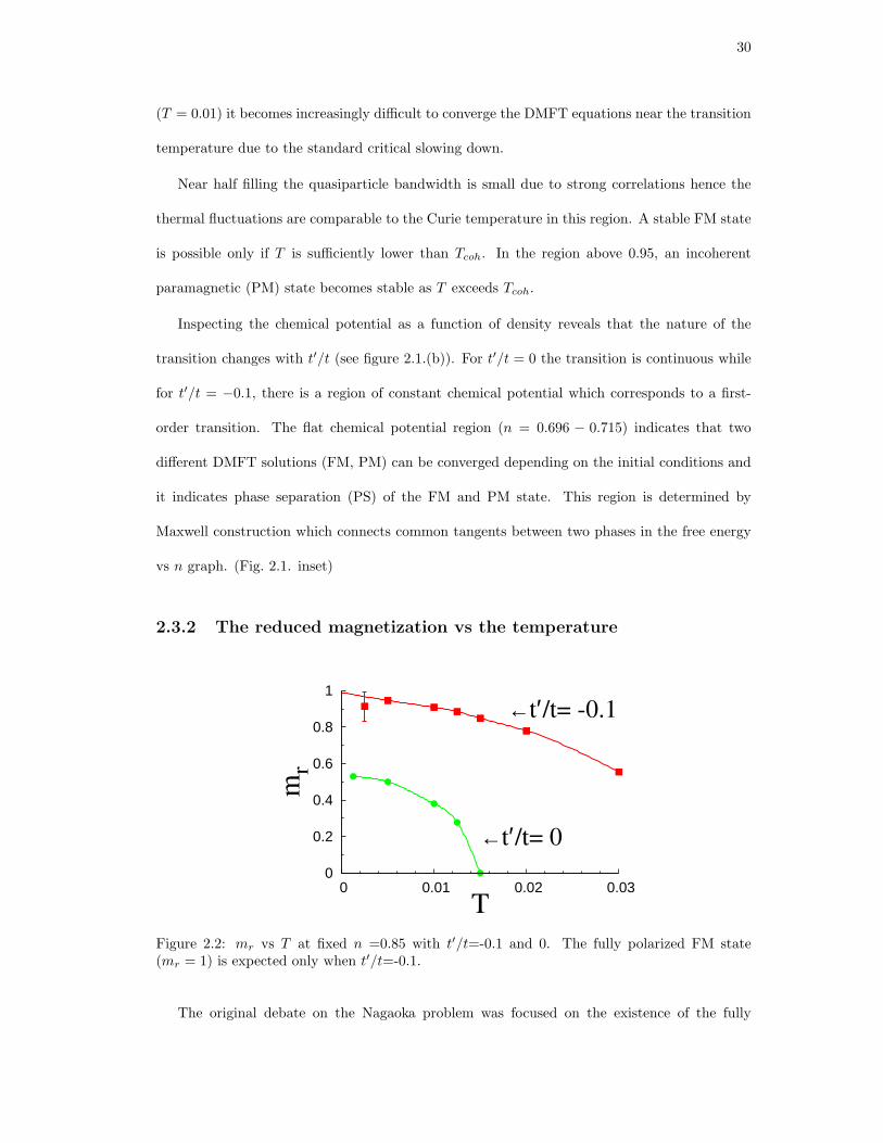
30

(T = 0.01) it becomes increasingly difficult to converge the DMFT equations near the transition

temperature due to the standard critical slowing down.

Near half filling the quasiparticle bandwidth is small due to strong correlations hence the

thermal fluctuations are comparable to the Curie temperature in this region. A stable FM state

is possible only if T is sufficiently lower than Tcoh. In the region above 0.95, an incoherent

paramagnetic (PM) state becomes stable as T exceeds Tcoh.

Inspecting the chemical potential as a function of density reveals that the nature of the

transition changes with t′/t (see figure 2.1.(b)). For t′/t = 0 the transition is continuous while

for t′/t = −0.1, there is a region of constant chemical potential which corresponds to a first-

order transition. The flat chemical potential region (n = 0.696 − 0.715) indicates that two

different DMFT solutions (FM, PM) can be converged depending on the initial conditions and

it indicates phase separation (PS) of the FM and PM state. This region is determined by

Maxwell construction which connects common tangents between two phases in the free energy

vs n graph. (Fig. 2.1. inset)

2.3.2 The reduced magnetization vs the temperature

0

0.2

0.4

0.6

0.8

1

0 0.01 0.02 0.03

mr

T

←t′/t= -0.1

←t′/t= 0

Figure 2.2: mr vs T at fixed n =0.85 with t′/t=-0.1 and 0. The fully polarized FM state(mr = 1) is expected only when t′/t=-0.1.

The original debate on the Nagaoka problem was focused on the existence of the fully

31

polarized FM state at finite δ in the T → 0 limit. Therefore, it is necessary to investigate

magnetization mr at very low T . In Fig. 2.2 we show very low temperatures (T = 0.001t)

results and it is clear that the magnetization saturates to a value smaller than unity for t′/t = 0

while it reaches unity at low temperatures for t′/t = −0.1. The fully polarized Nagaoka state

is thus not stable for t′/t = 0 and moderately small doping (δ ∼ 0.1) while it is realized for

t′/t = −0.1. As the spins become fully polarized (t′/t = −0.1, T → 0), numerics requires high

statistics and an error-bar is specified to take into account the numerical error.

2.3.3 The spectral function

The spectral functions are shown in Fig. 2.3. Since CTQMC delivers response functions on

the imaginary frequency axis, one needs to perform the analytical continuation of the Green

function to the real axis. Here we use the maximum entropy method [42]. The spectral functions

show noticeable differences for small change in t′. At t′/t = −0.1, the majority spin spectral

function shows a very small renormalization due to interactions (Z ≃ 1) and a large spectral

peak in the occupied part of the spectra. The overall shape is similar to the non-interacting

spectral function (Fig. 2.3. inset). The minority spin spectral function is much more correlated

and shows a narrow quasiparticle band above the Fermi level and a tiny lower Hubbard band.

In the magnetic state, the occupied part of the spectra is thus well described by a model of a

weakly correlated FM metal.

At t′/t = 0 and t′/t = 0.1, the spectral functions consist of both the narrow quasiparticle

band and the lower Hubbard band. In the U = ∞ Hubbard model, the upper Hubbard band

disappears due to the exclusion of double occupancy.

The stability of the FM state at t′/t = −0.1 can be traced back to the large spectral peak

in the occupied part of the spectra of the non-interacting DOS shown in the inset of Fig. 2.3.

As explained above, the majority spin of the FM state shows only weak renormalization due to

interactions. This is a consequence of the Pauli exclusion principle which constrains the motion

of a hole in the polarized background and interactions, being less important in this case, do not

32

0

0.2

0.4A

(ω)

t′/t= -0.1

majority

minority

0

0.5

1

-4 -2 0 2 4

A0(ω

)

ω−µ0

0

0.2

0.4

A(ω

)

t′/t= 0

0

0.5

1

-4 -2 0 2 4

A0(ω

)

ω−µ0

0

0.2

0.4

-4 -2 0 2 4

A(ω

)

ω

t′/t= 0.1

0

0.5

1

-4 -2 0 2 4

A0(ω

)

ω−µ0

Figure 2.3: The spectral functions A(ω) at t′/t=-0.1 (top), 0 (middle), and 0.1 (bottom) forfixed n =0.85. Inset: Non-interacting spectral functions (A0(ω)) of the majority spin at thecorresponding t′/t values. (µ0 = µ − ReΣ(0)) All calculations were performed at T=0.01.

33

hamper the coherent motion of the hole through the polarized background. The kinetic energy

of this state thus clearly depends on t′/t ratio and is reduced with decreasing t′/t. Contrary

to the FM state, the correlations are very strong in the PM state regardless of the spectral

peak in the non-interacting DOS and t′/t ratio. The coherent part of the spectra does not

contribute much to the kinetic energy as the quasiparticle bandwidth shrinks due to the strong

correlations. The incoherent part of the spectra in the form of the Hubbard bands arises from

localized electrons and consequently it is almost independent of the specific lattice dispersion.

Therefore, the kinetic energy of the PM state weakly depends on t′/t ratio. The peak in the

occupied part of the spectra of the non-interacting DOS thus reduces the kinetic energy of the

FM state compared to the PM state thus stabilizing ferromagnetism.

It is known from other studies [32] that a highly degenerate flat band in the occupied part

of the spectra favors ferromagnetism at any finite U . However, this flat band ferromagnetism

(an extreme limit of the Stoner ferromagnetism) argument is not applicable to the t′/t = −0.1

case of the Nagaoka ferromagnetism (the other extreme limit of the Stoner ferromagnetism).

In a flat-band model, the ground state of the non-interacting system is highly degenerate due

to the presence of the flat band. However, even a small Coulomb repulsion lowers the energy

of the FM state (if the flat band is half-filled) and stabilizes the FM state. The role of the

Coulomb interaction is simply to lift the huge degeneracy and ”select” the states with the

highest magnetization as unique ground states. In the infinite U model, the potential energy

vanishes because of no doubly occupancy. However, the kinetic energy depends sensitively on

the smoothness of the spin polarized background, and a disordered PM state can not gain the

kinetic energy by the variation of t′/t while a FM state can.

2.3.4 The uniform susceptibility

The inverse of the uniform magnetic susceptibility (χ−1q=0) of the PM state vs n at t′/t = 0 and

0.1 is shown in Fig. 2.4. The extrapolated line at t′ = 0 indicates that χ diverges near n = 0.815,

confirming the second order transition at the critical density (nc = 0.815). At t′/t = 0.1, one

34

0

0.02

0.04

0.06

0.08

0.1

0.7 0.8 0.9 1

χ q=

0−1

n

t′/t= 0t′/t= 0.1

Figure 2.4: The uniform susceptibility (χ−1q=0) vs n at t′/t = 0 and 0.1. The dotted line is for

the extrapolation to χ−1q=0 = 0. (T=0.01)

might expect χ will diverge near n = 1. However, as Tcoh becomes smaller than T near n = 1,

the incoherent PM state is stabilized. In other words, at t′/t = 0.1, the crossover from the

coherent PM state to the incoherent PM state occurs instead of the transition to the FM state.

2.3.5 The phase diagram

0

0.01

0.02

0.03

0.75 0.8 0.85 0.9 0.95 1

Tc

n

PM

FM

←Tcoh

Figure 2.5: The critical temperature Tc vs n at t′ = 0. nc at T = 0 is obtained from theextrapolation. The dotted line represents the coherence temperature Tcoh vs n.

Fig. 2.5 shows the critical temperature (Tc) vs n at t′/t = 0. In the region below Tc a

partially polarized FM state is found, and it is determined by observing n↑ 6= n↓ in a CTQMC

result. This graph shows that the lower critical density (nc) at T = 0 is around 0.8. At half

35

filling critical temperature should vanish due to the following reason: The kinetic energy at half

filling is zero in both the PM and the FM state because of the blocking of charge density. The

entropy of the paramagnet is much larger than the entropy of the ferromagnet due to the large

spin degeneracy of the PM state. In other words, PM state is thermodynamically stable at any

finite temperature at n = 1.

As the width of the quasiparticle band becomes smaller near n = 1, the coherence tem-

perature Tcoh is also reduced making it hard to sustain the quasiparticle coherent band. At

T > Tcoh, the PM state is clearly stabilized. The Tcoh boundary can be determined from the

imaginary part of self energy (ImΣ(iωn)) on the imaginary frequency axis. In a coherent re-

gion (T < Tcoh), the renormalization residue Z is well defined (0 < Z < 1) by evaluating the

negative slope of ImΣ(iωn) at ω = 0 (Z = (1 − dImΣdω |ω=0)

−1). However, in the incoherent

regime (T > Tcoh), the slope of ImΣ(iωn) at ω = 0 becomes positive making the concept of Z

ill defined (Fig. 2.7). Therefore, we determined Tcoh as the temperature where the slope of the

low energy self energy vanishes, and found that it is almost proportional to δ3/2, in surprising

agreement with the findings of a previous study of doped Mott-insulator [43].

In a two-dimensional Hubbard model, a long-range magnetic order at a finite T is prohibited

by the Mermin-Wagner theorem. A FM order is possible only at T = 0. At any finite T ,

Goldstone modes disorder the system [44], and it results in a correlation length which is finite

but exponentially large in T−1. DMFT does not capture this behavior. Therefore, Tc in the

context of the two dimensional model should be interpreted as an estimate of the temperature

where the correlation length gets very large. In higher dimensions, we expect a FM state at low

T with the correct dependence on t′/t. The Nagaoka ferromagnetism study using the dispersion

of realistic materials deserves further investigations since the energy balance between a FM state

and a PM state or the character of the transition is very sensitive to the details of the lattice

structure.

36

0

0.04

0.08

0.12

χ lo

c-1

n=0.75

n=0.85

n=0.95

0

0.02

0.04

0 0.01 0.02 0.03

χ q=

0-1

T

Figure 2.6: The local susceptibility (χ−1loc) vs T and the uniform susceptibility (χ−1

q=0) vs T(t′/t = 0)

2.3.6 The local susceptibility and the uniform susceptibility

In general, n↑ − n↓ exhibits small fluctuations near the boundary of Tc due to the finite T .

The fluctuations become especially severe through the transition from the FM state to the

incoherent PM state near n = 1. Therefore, the boundary points can be determined more

precisely by examining the temperature dependence of χ−1q=0 (Fig. 2.6). χ−1

q=0 near a transition

point obeys the Curie-Weiss form (χ−1q=0 ∼ T − Tc). Both coherent (n = 0.85) and incoherent

(n = 0.95) regions show linear dependence of χ−1q=0 on T . The χ−1

q=0 for n = 0.75 barely depends

on T , exhibiting Pauli paramagnetic behavior. χ−1loc is greater than χ−1

q=0 and it increases as n

decreases. This is because in DMFT χ−1loc ∼ T + Tcoh and Tcoh increases as n decreases [43].

2.3.7 The self energy

Fig. 2.7 shows the behavior of ImΣ(iωn) for the three different phases in the Tc phase diagram

of Fig. 2.5. For n = 0.85 and T = 0.01, a coherent FM state is expected from the phase diagram.

A coherent Fermi liquid is validated by investigating the negative slope of ImΣ(iωn) at ω = 0.

37

-4

-2

0

Im Σ

(iω

n)

n=0.85, T=0.01

minority

majority

-2

0

Im Σ

(iω

n)

n=0.85, T=0.02

-2

0

0 1 2 3 4

Im Σ

(iω

n)

iωn

n=0.95, T=0.02

Figure 2.7: ImΣ(iωn) vs iωn at the coherent FM state (the top panel), the coherent PM state(the middle panel), and the incoherent PM state (the bottom panel). (t′/t = 0)

38

The slope for spin σ at the high frequency part is given by −n−σ/1 − n−σ (Eq. 7) and the

inequality of the slope indicates n↑ 6= n↓ confirming the FM state. The majority spin state

has a smaller slope at high frequency because n−σ of the majority spin is smaller than that of

the minority spin. Also, because the slope of the majority spin at ω = 0 is smaller, Z of the

majority spin is larger than that of the minority spin. This means the quasiparticle band of the

minority spin is strongly renormalized by correlations while the majority spin state tends to be

similar to the non-interacting energy dispersion. For n = 0.85 and T = 0.02, a coherent PM

state is established by observing a negative slope at ω = 0 and no spin symmetry breaking. For

n = 0.95 and T = 0.02, an incoherent PM state is expected from the positive slope at ω = 0

because the concept of Z is no longer valid and the application of Fermi liquid theory fails.

Lastly, for fixed T = 0.02, as n increases from 0.85 to 0.95 the slope at high frequency also

increases because n−σ increases.

2.4 Nagaoka Ferromagnetism from a 4-site plaquette

-1.2

-1.1

-1

-0.9

-0.8

-0.4 -0.3 -0.2 -0.1 0 0.1 0.2 0.3 0.4

E

t′/t

S=3/2S=1/2

Figure 2.8: The lowest energies of a S=1/2 state and a S=3/2 state in a U = ∞ 4-site toymodel varying t′/t. E is the energy in units of t = 1/2.

In order to provide a simple interpretation of why decreasing t′ stabilizes the Nagaoka state,

we examine the simplest possible model which retains the physics of the Nagaoka problem. We

consider a 4-site plaquette with three electrons (one hole). The ground state of this model may

39

be characterized by the quantum number corresponding to the total spin angular momentum

(ie. S = 32 , 1

2 ) and the z-direction of the spin angular momentum (Sz = ± 32 , Sz = ± 1

2 ). The

whole Hamiltonian matrix is a 32 × 32 matrix excluding double-occupied sites and it is block-

diagonalized to 6 distinct spin sectors by performing the unitary transform to the proper S, Sz

basis. The ground state energy at each spin sector is determined by the exact diagonalization

of Hamiltonian matrix.

The lowest energy in a S = 32 sector is given by −2t + t′ and in the S = 1

2 sector is given

by −√

3t2 + t′2. The energy dependence of a S = 32 state is noticeably different from that of a

S = 12 . In a S = 3

2 case, doubly occupied states are excluded by the Pauli principle regardless

of U . Therefore, the U = ∞ Hamiltonian is equivalent to the U = 0 Hamiltonian where the

addition of the positive n.n.n hopping t′ contributes linearly to the increase of the kinetic energy.

However, doubly occupied states in a S = 12 sector are excluded only for U → ∞. Therefore,

unlike the S = 32 case, the energy dependence on t′ is greatly reduced as the Hilbert space

shrinks due to the infinite U .

A S = 32 ground state is indicative of the Nagaoka ferromagnetic state while a S = 1

2

ground state is indicative of a paramagnetic state. The S = 32 state is the ground state for

t′/t < 0.24 and the energy difference increases approximately linearly thereafter indicating that

the Nagaoka state is stabilized as t′/t is decreased. This is in qualitative agreement with the

DMFT results presented in the previous section. The energy of the S = 12 state weakly depends

on t′ while the S = 32 energy decreases as t′/t decreases. This also explains that the stability of

Nagaoka ferromagnetism originates from the minimization of the kinetic energy.

2.5 A mean-field slave boson approach

In this section, Nagaoka ferromagnetism in a U = ∞ Hubbard model is studied using a mean-

field slave boson approach. In a slave boson method, a fermion operator is accompanied by

bosonic operators (ie. slave bosons) which keep track of the local occupation number. The

three slave boson operators are e, p↑, p↓ and they act on unoccupied sites, spin-up sites, and

40

spin-down sites, respectively. In this U = ∞ case, the doubly occupied sites are excluded.

Constraints regarding the conservation of the occupation number are imposed with Lagrange

multipliers (λ, λ↑, λ↓). The slave boson Hamiltonian is given by

H = −∑

ijσ

tij c†iσ ziσ z†jσ cjσ −

∑

iσ

λiσ(p†iσ piσ − c†iσ ciσ) +

∑

iσ

λi(p†iσ piσ + e†i ei − 1) (2.10)

where ziσ = 1√1−p†

iσ piσ

e†i piσ1

q

1−e†i ei−p†

i−σ pi−σ

. tij=t if i,j are n.n, and tij=t′ if i,j are n.n.n.

The non-interacting ǫ(k) is taken to be −2t(cos kx +cos ky)− 4t′ cos kx cos ky as in the previous

section. The original Fock space has been enlarged including the slave boson fields. The par-

tition function can be calculated from the Feynman functional path integral over the original

fermi fields, slave boson fields, and Lagrange multipliers. The integral over the fermi fields is

straightforward because the Hamiltonian is quadratic in the fermi fields. The integral over the

slave boson fields and Lagrange multipliers should be performed using the saddle-point approxi-

mation, where the integral over the slave boson fields and Lagrange multipliers is approximated

by putting their space and time independent mean-field values which minimize the Hamilto-

nian. The physical meaning of slave boson mean-field value is clear. The expectation value

〈e†e〉 corresponds to the fraction of unoccupied sites, i.e. the hole density δ(1 − n). Similarly,

〈p†↑p↑〉 equals to the spin up occupation number (n↑), and 〈p†↓p↓〉 corresponds to the spin down

occupation number (n↓).

The free energy can be derived from the partition function (F = −kBT lnZ) and it is

necessary to compare the free energies between ferromagnetic state and paramagnetic state to

investigate the transition. The free energy is a function of magnetization m = n↑−n↓, δ, and T .

At T = 0, the free energy becomes the ground state energy. The energies of the fully polarized

ferromagnetic (FPFM) state (m = n↑) and the paramagnetic (PM) state (m = 0) are given by.

EFPFM (δ) =1

Ns

∑

k

ǫ(k)Θ(µ − ǫ(k)) (2.11)

EPM (δ) =1

Ns

∑

k,σ

Zǫ(k)Θ(µ∗ − Zǫ(k)) (2.12)

where Ns is the number of total sites, Z is the renormalization residue given by 2δ/(1+δ), µ is the

41

chemical potential in a fully polarized ferromagnetic state satisfying (1/Ns)∑

k Θ(µ − ǫ(k)) =

n↑ = 1 − δ, and µ∗ = (µ − λσ) is the effective chemical potential in a paramagnetic state

satisfying (1/Ns)∑

k Θ(µ∗ − Zǫ(k)) = n↑ = n↓ = (1 − δ)/2. The DOS of the FPFM state is

the same as the non-interacting DOS (ρ0(ǫ)) while the DOS of the PM state is renormalized

by a factor Z to 1/Z · ρ0(ǫ/Z). Unlike the DMFT method, the slave boson approach considers

only the renormalized quasiparticle DOS ignoring the incoherent contribution. EPM is given

by Z ·E0 where E0 is the non-interacting energy. In other words, as δ reduces to 0, the energy

for a paramagnetic state is strongly renormalized by a factor 2δ/(1 + δ) to avoid the doubly

occupied states. That makes the FPFM state more stable at small δ.

In Fig. 2.9.(a), FPFM energy and PM energy vs n are shown for t′/t = 0.1, 0 and −0.1. For

all values of t′/t, the FPFM energy is stable at large n while the PM energy is stable at small

n. The intermediate phase separated region is constructed by the Maxwell construction and is

indicative of a fist order transition. At large n, as in the plaquette case, the energy curve for the

paramagnet state depends weakly on t′ while the FPFM energy is reduced with decreasing t′/t.

This results is in qualitative agreement with the previous DMFT results. As t′/t decreases,

the FPFM state becomes more stable and the critical density, nc decreases. Just as in the

DMFT, the large spectral weight of the non-interacting DOS at a low energy makes FPFM

state energetically favorable at t′/t = −0.1. When t′ is 0, the energy difference between FPFM

and PM vanishes at nc=2/3, in agreement with the previous slave boson calculations [27, 28].

We also calculate the inverse of uniform magnetic susceptibility (χ−1) to study the instability

of the PM state. The analytic expression is

χ−1|m=0 =1

2ρ(µ∗)+

2µ∗

1 + δ+

1

Ns

∑

k

4

(1 + δ)2Zǫ(k)Θ(µ∗ − Zǫ(k)) (2.13)

where ρ(µ∗) is the renormalized DOS given by 1/Z · ρ0(µ∗/Z).

The trends in χ−1 are consistent with the results shown in Fig. 2.9.(a). As t′/t decreases,

spin susceptibility diverges at smaller density (see Fig. 2.9 (b)). However, the divergence of the

spin susceptibility does not coincide with the thermodynamic phase transition identified by the

total energy differences. The phase transition is thus always first order within the slave boson

42

-0.4

-0.2

0

E

(a)

t′/t= 0.1

FPFMPM

-0.25

-0.2

0.8 0.85

-0.4

-0.2

0E

t′/t= 0

-0.4

-0.35

0.65 0.7

-0.4

-0.2

0

E

t′/t= -0.1

-0.42

-0.4

0.5 0.55

-0.2

0

0.2

0.4

χ−1

(b) t′/t= 0.1t′/t= 0t′/t= -0.1

0

1

2

0.4 0.5 0.6 0.7 0.8 0.9 1

µ

n

(c) t′/t= 0.1t′/t= 0t′/t= -0.1

Figure 2.9: (a) Fully polarized ferromagnetic (FPFM) energy and paramagnetic (PM) energyvs n varying t′/t (0.1 (top), 0 (middle), and -0.1 (bottom)) Inset : Maxwell construction todetermine the PS region. (b) The inverse of the uniform magnetic susceptibility (χ−1) at m=0vs n varying t′/t (0.1, 0, and -0.1). (c) The chemical potential (µ) vs n at t′/t = 0.1, 0, and-0.1.

43

t′/t=-0.1 t′/t=0 t′/t=0.1DMFT nc 0.705 0.815 N/A

(T = 0.01) order First Second N/ASlave boson nc 0.53 0.67 0.83

(T = 0) order First First First

Table 2.1: nc and the order of the ferromagnetism transition in a U = ∞ Hubbard model fromboth the DMFT+CTQMC approach and the slave boson approach with t′/t= -0.1, 0, and 0.1.N/A means no transition to FM state occurs.

approach.

Fig. 2.9 (c) shows that a flat chemical potential region exists at any t′/ts in a µ vs n graph.

This is a generic feature of a first order transition and this region represents the coexistence of

the FPFM and PM phase. This coexistence region is larger for negative t′/t favoring transition

to the FPFM phase.

2.6 Comparison of the slave boson result and the DMFT+CTQMC

result

The slave boson method overestimates the region of the stable FM state as compared to DMFT

and it favors a first order transition (see Table 1). This is because the slave boson approach

overestimates the paramagnetic kinetic energy as compared to the DMFT approach (Fig. 2.10).

The quasiparticle residue Z of the DMFT approach is evaluated by (1 − dImΣdω |ω=0)

−1 on the

imaginary frequency axis while Z of the slave boson approach is given by 2δ/(1 + δ). Fig. 2.11

shows that Z of the slave boson study is overestimated as compared to the DMFT+CTQMC

case. The slave boson technique used in this chapter is based on the mean-field saddle-point

approximation and it does not treat the strong correlation effect properly. Even though DMFT

ignores the spatial correlation effect, the temporal correlations are treated exactly by CTQMC.

Moreover, the mean-field slave boson approach evaluates the total energy as the sum of coherent

quasiparticle energies (Eq. 2.12) while the total energy of DMFT+CTQMC includes contribu-

tions from both the incoherent and coherent effects. The over-estimated Z in the slave boson

case underestimates the kinetic energy while the ignorance of contribution from the incoherent

44

-0.4

-0.2

0

E

t′/t = -0.1

slave bosonDMFT

-0.4

-0.2

0

Et′/t = 0

-0.4

-0.2

0

0.6 0.7 0.8 0.9 1

E

n

t′/t = 0.1

Figure 2.10: Paramagnetic energy from both the DMFT+CTQMC (T = 0.01) and the slaveboson (T = 0) approach vs n at t′/t=-0.1 (the top panel), 0 (the middle panel), and 0.1 (thebottom panel).

0

0.1

0.2

0.3

0.4

0.5

0.6

0.65 0.7 0.75 0.8

Z

n

slave boson

DMFT

Figure 2.11: The renormalization residue (Z) of the slave boson method and theDMFT+CTQMC method (t′ = 0).

45

part overestimates the energy. As a result, the two errors of the slave boson approach cancel

each other giving a slightly overestimated energy as compared to the DMFT+CTQMC result.

Additionally, the χ−1 graph in the slave boson method almost coincides with the DMFT+CTQMC

result comparing Fig. 2.4 and Fig. 2.9 (b). It is not certain how the renormalization residue Z

affects χ−1 in the DMFT+CTQMC case, and the contribution from the incoherent part is also

unclear. Therefore, further study will be required to fully understand the positive agreement of

χ in the two methods.

2.7 Conclusion

To summarize, we investigated Nagaoka ferromagnetism in the U = ∞ Hubbard model including

n.n hopping t and n.n.n hopping t′. This model was solved using DMFT with CTQMC, and the

mean-field slave boson approach. Even a small value of t′/t yields a significant impact on the

stability of Nagaoka ferromagnetism. The DMFT results show that the FM state is more stable

for negative t′/t. This is supported by the slave boson method (see Table 1), and it can also

be understood from diagonalization of the 4-site plaquette. The energy of the minimum spin

state (S = 1/2) depends weakly on t′/t, while the energy of the maximum spin state (S = 3/2)

depends linearly on t′/t. Therefore, the maximum spin state becomes more stable for negative

t′/t.

In both the slave boson and DMFT methods, the paramagnetic energy does not vary much

with t′/t due to the strong renormalization of the quasiparticle band (see Fig. 2.10). How-

ever, the fully polarized ferromagnetic energy depends on t′/t in a similar fashion as the non-

interacting kinetic energy since the correlations are weaker in the broken symmetry state. The

negative t′/t gives a high spectral peak in the occupied part of the spectra of the non-interacting

system. As a result, the energy of the FM state is lower, and the ferromagnetism is stabilized

in this case.

Within DMFT, the nature of the transition also varies with t′/t. A first order transition

accompanied by the PS of the FM and PM state occurs at t′/t = −0.1 while a second order

46

transition occurs at t′/t = 0. In the slave boson approach, the transition is always first order

regardless of t′/t. This is because the slave boson method overestimates the PM energy. The

DMFT result shows that when n → 1, the FM state becomes unstable as T exceeds Tcoh. In

other words, the ferromagnetic state is only stable within the coherent Fermi liquid regime.

The U = ∞ one band Hubbard model is a toy model and does not describe any specific

material. However it is physically realizable in an optical lattice, due to the recent developments

in controlling cold atoms in optical traps [45, 46]. These systems are highly tunable, and the

hopping parameter t and the on-site interaction U can be adjusted by varying the ratio of the

potential depth of the optical lattice to the recoil energy (V0/ER) or the ratio of interatomic

scattering length to the lattice spacing (as/d). In order to realize the one-band Hubbard model

with a large U (U/t ≥ 100), V0/ER ≈ 30 and as/d ≤ 0.01 should be the range of parameters

in the optical lattice (See Fig. 4 of Ref. 29). The tuning of the next-nearest neighbor hopping

t′ can be achieved by engineering optical lattices with a non-separable laser potential over each

coordinate axis.

It will be very interesting to test these DMFT results experimentally. Usually, the atomic

trap potential is applied to confine atoms in the optical lattice, and the potential varies smoothly

having the minimum at the center of the trap. The phase separation between the FM and the

PM phase at t′/t = −0.1 (taking place between the densities n = 0.696−0.715) can be observed

in the optical lattice as three spatially separated distinct regions. The atom-rich FM region will

tend to move to the center of the optical lattice to be energetically stabilized while the hole-rich

PM region will reside on the edge of the optical lattice. Since the total spin is a conserved

quantity, the FM region will be located at the center of the trap and will consist of two domains

containing the up or down species. Raising the temperature will destroy the ferromagnetic

magnetic state and, consequently, the spatial patterns within the trap.

47

Chapter 3

Cluster Dynamical Mean Field Theory of the Mott

Transition

In this chapter, we address the nature of the Mott transition in the Hubbard model at half-filling

using cluster Dynamical Mean Field Theory (DMFT) [47]. We compare cluster DMFT results

with those of single site DMFT. We show that inclusion of the short range correlations on top

of the on-site correlations, already treated exactly in single site DMFT, does not change the

order of the transition between the paramagnetic metal and the paramagnetic Mott insulator,

which remains first order. However, the short range correlations reduce substantially the critical

U and modify the shape of the transition lines. Moreover, they lead to very different physical

properties of the metallic and insulating phases near the transition, in particular in the region of

the phase diagram where the two solutions coexist. Approaching the transition from the metallic

side, we find an anomalous metallic state with very low coherence scale but relatively large

quasiparticle renormalization amplitude at temperatures as low as T = 0.01t. The insulating

state is characterized by the relatively narrow Mott gap with pronounced peaks at the gap edge.

The transition from the insulating side is characterized by the continuous closure of the Mott

Hubbard gap.

3.1 What is the Mott transition?

The correlation driven metal insulator transition is one of the most fundamental problems

in condensed matter physics, and continues to receive intensive attention. It is realized in

numerous transition metal oxides and some organic salts, by application of the pressure or

isovalent chemical substitutions [48]. The metallic state far from the transition is well described

48

by the Fermi liquid theory, illustrating the wave-like properties of electrons in solids. In the

insulating side, the electron behaves as a localized particle. Near the transition, the effective

Coulomb repulsion between the carriers is of the same order as the kinetic energy term in

the Hamiltonian. This regime probes the dual character of electron, namely the particle- and

wave-like character, and requires a non-perturbative method for its description.

The nature of the metal to insulator transition depends strongly on the degree of magnetic

frustration. In the limit of very large magnetic frustration, the insulating state is a simple

paramagnetic state with local moments carrying log(2) entropy. The metallic state is a Fermi

liquid with a very heavy mass. The mass increases as the transition is approached to match the

large entropy of the frustrated paramagnetic insulator. This is the essence of the Brinkman-

Rice theory of the metal insulator transition, which has been substantially extended by the

single site DMFT of the Hubbard model in the paramagnetic phase [7]. The key predictions of

this approach, such as the existence of a first order line ending in a second order Ising point,

and numerous high temperature crossovers, have been verified experimentally [49]. The first

order phase transition in a strongly frustrated situation has been confirmed by cluster DMFT

studies [50, 51] and by other techniques [52].

The completely unfrustrated case is also well understood along the lines first drawn by Slater,

and realized in the half filled one band Hubbard model with only nearest neighbor hoppings.

Here, the metal insulator transition is driven by the long range magnetic ordering. The system

is insulating and magnetic for arbitrarily small values of U, as a reflection of the perfect nesting

of the band structure. The insulating gap results from the formation of a spin density wave

that Bragg scatters the electronic quasiparticles.

The character of the metal insulator transition with an intermediate degree of frustration

(when the long range magnetic order is fully suppressed, but with strong short range magnetic

correlations) remains an open problem. Qualitative modifications of the character of the tran-

sition are expected, since at low temperatures the paramagnetic insulating state has very low

entropy. This problem can be addressed by a sharp mathematical formulation studying the

49

paramagnetic solution of the cluster DMFT equations of the Hubbard model, keeping the short

range correlations only. The early cluster DMFT studies received conflicting answers depending

on different cluster schemes and different impurity solvers [53, 54]. However, by going to very

low temperatures using new algorithmic developments, we completely settle this question.

3.2 The cluster DMFT Method

In order to study this problem of the Mott transtion, we apply cellular dynamical mean field

theory (CDMFT) [55, 56] to the two-dimensional Hubbard model. The Hubbard model is an

effective model which can treat the competition between the kinetic energy and the potential

energy of electrons in the lattice. The kinetic energy term originates from the hopping (t) of

fermions to adjacent sites and the potential energy term is the on-site Coulomb energy (U)

of doubly occupied electrons. The metal to insulator transition is controlled by the ratio U/t.

Here, we choose the two dimensional square lattice with only the nearest neighbor hopping t.

H = −t∑

i,j,σ

f†i,σfj,σ + U ·

∑

i

f†i,↑f

†i,↓fi,↓fi,↑ (3.1)

Cluster DMFT is an extended version of DMFT as it maps the lattice problem to an auxiliary

cluster quantum impurity problem embedded in a self-consistent electronic bath. The short-

range correlations ignored within DMFT can be captured within cluster DMFT inside the

cluster size. CDMFT, one scheme of cluster DMFT, uses plaquette as a reference frame and the

lattice problem is divided into 2 × 2 plaquettes for the problem treated here. Equivalently, the

original unit cell of a single site increases to a 2× 2 supercell. As a result, the original Brillouin

zone is reduced by half and the quantities within the supercell depends on the cluster degrees

of freedom.

The matrix of tight-binding hoppings tc(k) is a 4 × 4 matrix defined on the cluster degrees

of freedom. k runs over the reduced Brillouin zone of the problem. tc(k) can be given on the

real space basis within the cluster. In the 2 × 2 cluster, the real space vector R=(0,0), (1,0),

50

(0,1), and (1,1). tc(k) for the square lattice in Eq. 3.1 is given as follows.

tc(k)R1,R2=

0 −t(1 + eikx) −t(1 + eiky ) 0

−t(1 + e−ikx) 0 0 −t(1 + eiky )

−t(1 + e−iky ) 0 0 −t(1 + eikx)

0 −t(1 + e−iky ) −t(1 + e−ikx) 0

(3.2)

This hopping matrix can be Fourier transformed to a cluster momenta (K) basis. The

cluster momenta K are (0,0),(π,0),(0,π), and (π,π) within the 2 × 2 cluster. Within CDMFT,

the translation symmetry is broken inside the cluster, hence the off-diagonal terms appears in

the hopping matrix.

tc(k)K1,K2=

1

Nc

∑

R1,R2

ei(K1·R1−K2·R2) · tc(k)R1,R2(3.3)

tc(k)K1,K2=

ǫ0(k) i · ǫ2(k) i · ǫ3(k) 0

−i · ǫ2(k) ǫ1(k) 0 i · ǫ3(k)

−i · ǫ3(k) 0 −ǫ1(k) i · ǫ2(k)

0 −i · ǫ3(k) −i · ǫ2(k) −ǫ0(k)

(3.4)

where ǫ0(k) = −t(2 + cos(kx) + cos(ky)), ǫ1(k) = t(cos(kx) − cos(ky)), ǫ2(k) = t sin(kx), and

ǫ3(k) = t sin(ky).

The cluster self energy Σc treats electron correlations within the cluster size exactly but

inter-correlations between clusters are ignored within CDMFT. The 2×2 cluster is special since

Σc is diagnoal on the cluster momenta basis as the inter-cluster self energies are ignored.

Σc =

Σ00

Σπ0

Σ0π

Σππ

(3.5)

The cluster Green’s function Gc is also diagonal on the cluster momenta basis since the off-

diagonal terms originating from the hopping matrix in Eq. 3.4 vanishes as Gc is averaged over

51

the k points in the reduced Brillouin zone. Therefore, cluster momenta are the good quantum

number in 2 × 2 CDMFT and the other cluster quantities can be also given on the cluster

momenta basis.

Similar as DMFT, a self-consistent hybridization ∆c is determined from the condition the

cluster Green’s function Gc is same as the impurity Green’s function computed from an im-

purity solver with the impurity hybridization ∆c. The cluster quantities, ∆c, Gc, and Σc are

represented by an 8×8 diagonal matrix in the cluster momenta space including the spin degrees

of freedom. The hopping matrix tc(k) is given in Eq. 3.4. Finally, the self-consistent condition

for ∆c is determined as the following equation.

∆c(iω) = iω + µ − Σc(iω) − G−1c

= iω + µ − Σc(iω) −

1

Nk

∑

k

1

(iω + µ) · 1 − tc(k) − Σc(iω)

−1

(3.6)

where 1 is an identity matrix and k runs over the reduced Brillouin zone.

The cellular DMFT approach has already given numerous insights into frustrated models

of kappa organics [57, 50] as well as the doping driven Mott transition in the Hubbard model,

when treated with a variety of impurity solvers [58]. Here, we summarize briefly other recent

studies of the metal insulator transition in the Hubbard model using cluster DMFT. In Ref. [53] a

different type of cluster scheme, dynamical cluster approximation, was employed and the Hirsch-

Fye quantum Monte Carlo method was used as the impurity solver. The lowest temperature

reached was too high to see the metal insulator transition in small clusters. In this study, only

the largest cluster of size 64 was able to identify a gap at the value of U comparable to our

critical U . In Ref. [50], the first order metal-insulator transition was found for Kagome lattice at

large frustration t′=0.8t. The shape of the phase diagram is consistent with our phase diagram

in Fig. 3.1 but the temperature scale, at which the transition was identified, is factor of three

larger than found in our study. This is likely due to different type of band dispersion employed

in their work. This work also used the Hirsch-Fye quantum Monte Carlo method.

In our study, the auxiliary cluster problem is solved with the numerically exact continuous

52

time quantum Monte Carlo (CTQMC) method [17, 16]. CTQMC allows us to reach very low

temperature compared to the previous studies and the character of the Mott transition within

cluster DMFT is clearly revealed. The cluster DMFT results are explained in the following

section.

3.3 Cluster DMFT results

3.3.1 The phase diagram

Fig.3.1a shows the phase diagram of the Hubbard model within cluster DMFT at half-filling in

the absence of long range order. For interaction strength U < Uc2(T ), we find a metallic solution

while for U > Uc1(T ), a Mott insulating solution exists. The two transition lines Uc1(T ) and

Uc2(T ) cross at a second order endpoint, at temperature TMIT ∼ 0.09t and interaction strength

UMIT ∼ 6.05t. It is clear that one of the most salient features of the single site DMFT phase

diagram (shown in Fig. 3.1b), namely the existence of a first order phase transition, survives in

plaquette-DMFT.

Still there are substantial modifications to the single site DMFT results when U/t is close

to its critical value. Namely,

1. Strong short ranged antiferromagnetic correlations significantly reduce the value of critical

U at which the second order endpoint occurs. Note that the plaquette-DMFT critical

U(∼ 6.05t) is in very favorable agreement with the Monte-Carlo crossover U at which

the pseudogap develops at intermediate temperatures accessible by determinantal Monte

Carlo (figure 5 in Ref. [59]). This critical U will increase if the system is more frustrated

at short distance. For example, the inclusion of the next nearest hopping t′ has this effect

and was studied in Ref. [60].

2. The shape of the coexistence region, where both metallic and insulating solutions exist, is

significantly different. The high temperature crossover lines (dashed line above T ∼ 0.1t

in Fig.3.1) are similar since at high temperature the entropy of the paramagnetic insulator

53

-0.2 -0.1 0.0 0.1 0.2r t/U

0.00

0.05

0.10

0.15

0.20

0.25

t/T

Fermi

liquid

Paramagnetic

insulator

Bad

metal

Bad

insulator

1cU

2cU

TIMU

a)

plaquette

T/t=0.01 T/t=0.3

-0.2 -0.1 0.0 0.1 0.2r t/U

0.00

0.05

0.10

0.15

0.20

0.25

t/T

Fermi

liquid

Paramagnetic

insulator

Bad

metal

Bad

insulator

b)

single site

Figure 3.1: a) The phase diagram of the paramagnetic half-filled Hubbard model withinplaquette-CDMFT. Inset: The histogram of the two insulating states. It shows the proba-bility for a given cluster eigenstate among the 16 eigenstates of the half-filled plaquette. Thesinglet plaquette ground state has the highest probability. b) For comparison, the correspond-ing phase diagram of the single site DMFT (using the same 2D density of states) is shown.The coexistence region is shown as the shaded region. The dashed line marks the crossoverabove the critical point. The crossover line was determined by the condition that the imaginarypart of the self-energy at few lowest Matsubara frequencies is flat at the crossover value of U .For easier comparison, the x-axis is rescaled and the reduced value of Ur = U−UMIT

UMITis used.

The critical value of U is UMIT = 6.05t in cluster case and UMIT = 9.35t in single site case.Pentagons in panel a) mark the points in phase diagram for which we present the local spectralfunctions in Fig.3.2.

54

is of the order of log(2) in both cluster and single site approach. As the temperature is

increased, the large entropy insulating state wins over the lower entropy metallic state.

At low temperature, the situation is very different. In single site DMFT, the metal

wins at low temperature in the transition region because the emergence of the itinerant

quasiparticle inside the Mott gap lowers the free energy of the strongly disordered Mott

state. In the cluster case, the Mott insulator at very low temperature is very different

and has small entropy due to short range singlet formation. The small entropy of this

state can be confirmed by the ”valence histogram” shown in the inset of Fig.1a. The

high temperature insulating state, which has entropy of the order of log(2), populates

many states of the plaquette with significant probability. In contrast, there is only one

significant eigenvalue of the density matrix in low temperature, corresponding to the

singlet state. The insulating phase at low temperature has thus very small entropy, and

the bad metal has larger entropy, hence decreasing temperature favors insulator over metal.

The actual first order line (dashed line in Fig. 3.1a inside the coexistence region, where the

free energy of the two phases equals) therefore bends back and critical U decreases with

decreasing temperature. It is apparent that the zero temperature transition in cluster-

DMFT happens at Uc1 and not at Uc2 as in DMFT.

While the shape of the DMFT phase diagram strongly resembles the phase diagram of

the Cr-doped V2O3, the reentrant shape of the cluster-DMFT transition resembles more the

κ−organic diagram [61] as pointed out in Ref. [50]. The well known reentrant behavior of

these systems might be qualitatively understood within this approach. If the temperature is

varied at fixed pressure (here fixed U/t) the system is Mott insulating at very low temperature,

becomes metallic at intermediate temperature and insulating again at high temperature. In our

model, the short range spin-fluctuations stabilize the Mott state at low T , while metallic phase

intervenes at intermediate temperature where the local singlet formation is less efficient than

quenching of local moment by Kondo effect. Finally at high temperature the large entropy local

moment state wins and the system is again insulating.

55

3.3.2 The spectral function

0.0

0.1

0.2)ω(

AU/t=5.0a) U/t=5.4b)

-4 -2 0 2 4ω

0.0

0.1

0.2

)ω(

A

U/t=5.6c)

-4 -2 0 2 4ω

U/t=5.8d)

Figure 3.2: The local spectral function for four representative values of U/ts and temperatureT = 0.01t marked by pentagons in Fig.1. a) For U below Uc1 the system is in Fermi liquidregime with rather large coherence temperature. b) In the coexistence region, the insulatingsolution has a small but finite gap (∼ 0.2t). c) The metallic solution in the same region isstrongly incoherent and the value at zero frequency decreases due to the finite scattering rate(see self-energy in Fig. 3.3a). d) For U above Uc2, the Mott gap steadily increases with U .In addition to the Hubbard bands, quite pronounced peaks at the gap edge can be identified.Similar peaks can be seen also in single site DMFT, but they are substantially more pronouncedhere due to the small size of the gap within CDMFT.

To understand the effects brought about by the short range magnetic correlations near the

transition, we focus on the local spectral functions displayed in Fig. 3.2. As in single site

DMFT, below Uc1 (Fig. 3.2a) the system is a normal Fermi liquid with a reduced width of the

quasiparticle peak (Z ∼ 0.4) and well developed Hubbard bands around −2.5t and 2.5t.

The insulator in the coexistence region (Fig. 3.2b) is however very different than Mott

insulator in single site DMFT. The Mott gap is small and it vanishes at Uc1 where the insulating

solution ceases to exist. At low temperature very pronounced peaks at the gap edge appear.

These peaks are a clear hallmark of the coherence peaks characteristic of a Slater spin density

wave. This has been noticed earlier in numerous studies of the Hubbard model [62, 63, 54], as

well as in the single site DMFT solution in the ordered phase of the unfrustrated lattice, which

56

captures the physics of perfect nesting.

With increasing U above Uc2 (Fig. 3.2d) the Mott gap increases but the peaks at the gap

edge remain very pronounced. Only at very large U comparable to the critical U of the single

site DMFT they lose some of their strength and dissolve into a featureless Hubbard band.

The metallic state, which competes with the insulator in the coexistence region, (Fig. 3.2c)

has similar width of the quasiparticle peak as the Fermi liquid state at U < Uc1. Hence the

quasiparticle renormalization amplitude, as extracted at finite but low temperature T = 0.01t

is rather large. On the other hand, this metallic solution has somewhat reduced height of the

quasiparticle peak which is mostly due to incoherent nature of the solution.

At the heart of the cluster DMFT physics is the competition between the formation of an

itinerant band and short range spin fluctuations. The latter are absent in single site DMFT

since only the local moment formation is accounted for by DMFT. The competition between

spin fluctuations and Kondo screening leads to two important effects: i) the metallic state is a

strongly incoherent metal, ii) the quasiparticle renormalization amplitude Z as will be shown in

Fig. 3.4 is finite at the metal insulator transition and the Brinkman-Rice scenario of diverging

effective mass is absent in this model.

3.3.3 The cluster self energy

The incoherence can also be identified from the raw data on the imaginary axis. In Fig. 3.3

we show the imaginary self-energy for the different cluster momenta K, which can be thought

as the orbitals of the multi-orbital model associated with the cluster. In plaquette geometry,

the self-energy is diagonal in cluster momentum base and the on-site, nearest-neighbor, and

next-nearest-neighbor self-energies can be constructed as the linear combination of these orbital

self-energies[58].

Below Uc1, the self-energies of all four orbitals are very similar and results are close to the

single-site DMFT. The metallic phase in the coexistence region Fig. 3.3c has a large scattering

rate in the (π, 0) orbital, in the orbital which contributes most of the spectral weight at the

57

-1.0

-0.5)ωi(

ΣmI

U/t=5

Fermi liquid

a))0,0(=K

)0,π(=K

0.0 0.5 1.0ωi

-1.0

-0.5

)ωi(

ΣmI

U/t=5.6

incoh. metal

c)

-3

-2

-1

insulator

U/t=5.4

b)

0.0 0.5 1.0ωi

-3

-2

-1

insulator

U/t=5.8

d)

4.5 5.0 5.5 6.0 6.5t/U

-3

-2

-1

0

1

2

3

µ−)

− 0(Σe

R

e)

metal insulatorcoex

)0,0(=K

)π,π(=K

)0,π(=K

Figure 3.3: top: The imaginary part of the cluster self energies for the same parameters as inFig.2. Due to particle-hole symmetry, the (π, π) and (0, 0) cluster self-energies have the sameimaginary part and we show only one of them. Below the metal-insulator transition shown herein a), the momentum dependence of the self-energy is rather weak and the cluster solution is verysimilar to the single site DMFT solution. In the coexistence region, the metallic solution shownhere in c) is strongly incoherent especially in the (π, 0) orbital. For the insulating solutions inb) and d), the (π, 0) scattering rate diverges which opens the gap in the spectra. bottom: e)ReΣK(0−) − µ as a function of U . Due to particle-hole symmetry, ReΣK=(π,0) − µ vanishes.

58

fermi level. The coherence scale in this strongly incoherent metal is thus severely reduced. The

scattering rate as a function of temperature is not quadratic even at T = 0.01t and remains

large ∼ 0.2t at that temperature.

In Fig. 3.3b,d the Mott insulating state can be identified by the diverging imaginary part

of the Σ(π,0)(iω). Due to particle hole symmetry, the real part of the same quantity vanishes.

Therefore, the only way to open a gap in the single particle spectrum is to develop a pole at

zero frequency Σ(π,0) ≃ C/(iω). We checked that the insulating state in the coexistence region

has the characteristic 1/(iω) behavior at very low temperature and the coefficient C in the

coexistence region decreases as U decreases. The closure of the gap at the Uc1 transition point

is confirmed by the vanishing of C at that point.

The other two orbitals expel their Fermi surfaces by a different mechanism identified in

Ref. [64], namely the real parts of the self-energy are such that the effective chemical potential

µeff = µ−Σ(0−) moves out of the band. The separation of the two orbitals gradually increases

as U increases, and it jumps at the critical U showing the hysteresis behavior displayed in

Fig. 3.3e.

3.3.4 The quasi-particle resudue Z

The important issue in the metal insulator transition (MIT) is whether the short range magnetic

exchange in the Hubbard type of models allow the Brinkman-Rice scenario of diverging effective

mass. In Fig. 3.4 we plot the quasiparticle renormalization amplitude Z of the four different

orbitals of the plaquette. As shown in Fig. 3.4, the growth of the effective mass in cluster

DMFT is cut-off by the exchange interaction and the spatial coherence is lost way before the

quasiparticles acquire a large effective mass. The lattice Zk is a linear combination of the

two values plotted in Fig. 3.4. The quasiparticles at (π, 0) and (0, π) are renormalized more

strongly than those away from the two points. More importantly, close to Uc1, where the system

is still coherent at T = t/100, the quasiparticle renormalization amplitude is rather large for

the plaquette without frustration (Z ∼ 0.36). Very near and inside the coexistence region, the

59

4 5 6 7 8 9 10 11U/t

0.0

0.1

0.2

0.3

0.4

0.5

0.6

0.7

Z

meta

l

insula

tor

coex

)π,0(,)0,π(=K

)π,π(,)0,0(=K

TFMD

Figure 3.4: The quasi-particle residue Z vs U/t for different orbitals in CDMFT. Below thetransition point, the (0, 0) and (π, π) orbitals have essentially the same Z as single site DMFT(dotted line) while the quasiparticles are more renormalized in (π, 0) orbital. At the transition,both Z’s are rather large (0.36 and 0.48).

metallic state remains very incoherent at our lowest temperature T = t/100. We therefore can

not determine the low energy Z which might vanish at Uc2 at zero temperature.

3.4 Conclusion

In conclusion, we used essentially exact numerical method, CTQMC and clarified the nature of

the Mott transition in cluster DMFT. The short range correlations, which are accounted for in

this study but are absent in single site DMFT, do not change the order of the Mott transition,

which remains first order with coexistence of metallic and insulating solutions.

Our cluster DMFT study predicts the existence of an anomalous metallic state within the

coexistence region with very low coherence temperature. This regime could be relevant to the

interpretation of experiments in V O2 [65] and PrNiO3 under the applied pressure [66] where an

anomalous metallic state was reported. Recent optical measurements of V O2 [65] show that in

the narrow temperature range close to the transition, where the system percolates, the metallic

puddles show an unconventional optical response. The resistivity measurement of PrNiO3 under

60

the applied pressure [66] report the non-Fermi liquid metallic state near the Mott transition

boundary.

On the theoretical side, the plaquette DMFT brings new light on the nature of the in-

teraction driven MIT. The cluster DMFT of this problem retains aspects of Mott physics, as

described in single site DMFT, and Slater physics. It does that by having two orbitals ((π, 0)

and (0, π)) exhibit a Mott transition while the remaining orbitals ((0, 0) and (π, π)) undergo a

band transition. This Slater-Mott transition requires momentum space differentiation and has

no analog in single site DMFT.

61

Chapter 4

The Calculation of Two-particle Quantities within

DFT+DMFT

In this chapter, we derive the equations for computing the magnetic/charge susceptibility and

the superconducting pairing susceptibility using the two-particle vertex functions based on

DMFT. First, we discuss the advantages of the vertex function approach for computing the

two-particle response functions compared to the alternative cluster DMFT method. And the

Monte Carlo sampling procedure of the two-particle Green’s function χ by continuous time

quantum Monte Carlo (CTQMC) is explained in the next section. Since χ sampled by CTQMC

is reliable only at low frequency, we propose an extrapolation method based on singular value

decomposition for the high frequency values of χ. Using this sampled χ, the magnetic/charge

susceptibility can be computed using the Bethe-Salpeter equation in the particle-hole channel.

Finally, we derive the equations for computing the pairing vertex based on DMFT vertex func-

tions. The pairing vertex represents the pairing interaction between the electrons in a Copper

pair. The critical temperature (Tc) and the gap symmetry of superconductivity can be deter-

mined by computing the leading eigenvalue and the corresponding eigenfunction of the pairing

matrix in the particle-particle channel.

4.1 Motivation for the vertex function approach

Dynamical Mean Field Theory (DMFT) is a powerful theory for computing the electronic

structure of strongly correlated solid state systems [7, 67]. It maps the problem of a solid to an

auxiliary impurity problem where the local correlations are treated exactly while the non-local

correlations are ignored. In this way, both the coherent quasi-particle bands and the incoherent

62

Figure 4.1: Two routes for treating the non-local correlations beyond DMFT.

atomic like excitations are captured by this method. In combination with Density Functional

Theory (DFT), DMFT has been successful in describing the correlated electronic structure of

many realistic materials including the multiple valences in plutonium [68], the coherence scale

of CeIrIn5 [69], the correlated band structure of the Fe based high Tc superconductors [70] and

many others.

In some cases, non-local correlations are vital to describe the exotic phenomena qualitatively

different from the local physics described within DMFT. To name just a few examples: i) the

Mott transition accompanied by the antiferromagnetic correlations which result in a different

topology of the phase diagram [47], ii) the d-wave superconductivity in models of cuprates

arising from the spin fluctuations [71, 58], iii) the Mott transition at the optimal doping of the

Hubbard model [72] accompanied by the signs of quantum criticality [73, 74]. This non-local

correlations, not captured by DMFT, can be described by two types of the extensions of DMFT

(see Fig. 4.1).

One popular route is to extend the spatial range in which the correlations are treated exactly.

These cluster DMFT methods [55, 56] result in an auxiliary impurity problem spanning a cluster

of sites. The bottleneck of this approach is that the solution of the resulting quantum impurity

problem becomes computationally very expensive with increasing cluster sites. The number

of atomic states grows exponentially as 4Nb∗Ns where Nb is the number of bands and Ns is

the number of cluster sites. Therefore, the cluster DMFT approach is difficult to extend to

63

multi-orbital systems in realistic materials.

The second route of including non-local correlations is to use diagrammatic approaches

employing the n-particle vertex functions. In the limit of the infinite dimension z, the self

energy contains only local diagrams [7]. The next leading non-local diagram of the self energy

scales as 1/√

z and this type of diagram can be constructed through the use of the momentum

dependent propagators while the irreducible two-particle vertex function is assumed to be purely

local [75, 76]. Generally, the irreducible n-particle vertex function needs to be assumed to be

local for the higher order non-local contribution to the self energy.

DMFT can be thought as the lowest order version of the vertex function approach, since

the self energy, i.e., the one-particle irreducible vertex function is assumed to be local. As n

increases, more diagrams are treated with the non-local propagators and the exact solution is

recovered when n goes to infinity. In this approach, the vertex functions of lower order than

n include the non-local correlations along with long-range correlations. In contrast, within

cluster DMFT the long range correlations beyond the cluster size are ignored. Moreover, the

vertex function calculation is rather inexpensive compared to the cluster DMFT method since

it requires a solution of only the single-site quantum impurity problem, but it does require

the computation of higher order correlation functions of the quantum impurity problem. This

approach is a promising route to treat the non-local correlation in realistic strongly correlated

materials. It has been recently used to compute the magnetic susceptibility of the Fe based

superconductor within the DFT+DMFT approach [77].

In this chapter, we derive formulas for the vertex function approach to compute the two-

particle response functions such as the magnetic susceptibility and the superconducting pairing

susceptibility. This approach is derived here for the multi-orbital case and was implemented

within the DFT+DMFT method as a part of this thesis.

64

4.2 Sampling of the two-particle Green’s function

In Section1.4, we showed that the one-particle Green’s function is constructed by removing one

row and one column in the hybridization matrix ∆k. In similar way, the two-particle Green’s

function can be sampled by removing two rows and two columns in the hybridization matrix

∆k. The average of the four time-ordered fermionic operators can be obtained by taking the

derivative of lnZ with respect to the elements of ∆ twice, similar as in Eq. 1.57, i.e.,

χ sqpr

(τp, τq, τ′r, τ

′s) = 〈Tτψ†

αp(τp)ψ

†αq

(τq)ψα′r(τ ′

r)ψα′s(τ ′

s)〉

=∂2 lnZ

∂∆αpα′s(τp, τ ′

s)∂∆αqα′r(τq, τ ′

r)(4.1)

If we take the same derivative of the Taylor expansion form in Eq. 1.50, we get

χ sqpr

(τp, τq, τ′r, τ

′s) =

∂

∂∆αpα′s(τp, τ ′

s)

(∂ lnZ

∂∆αqα′r(τq, τ ′

r)

)

=1

Z

∫D[ψ†ψ]e−Sc ·

∑

k

1

k!

∫ β

0

dτ1

∫ β

0

dτ ′1 · · ·

∫ β

0

dτk

∫ β

0

dτ ′k

∑

α1α′1,··· ,αk,α′

k

ψα′1(τ ′

1)ψ†α1

(τ1) · · ·ψα′k(τ ′

k)ψ†αk

(τk)

× 1

k!

∂

∂∆αpα′s(τp, τ ′

s)

(∂Det(∆k)

∂∆αqα′r(τq, τ ′

r)

)(4.2)

The derivative of the determinant of the matrix ∆k with respect to two independent matrix

elements is equivalent to removing two rows and two columns containing the two elements. We

denote the resulting (k − 2) × (k − 2) matrix by (∆k)′′pqrs,

∂

∂∆αpα′s(τp, τ ′

s)

(∂Det(∆k)

∂∆αqα′r(τq, τ ′

r)

)= (−1)p+q+r+s · Det((∆k)′′pqrs) (4.3)

65

and it takes the form

(∆k)′′pqrs ≡

∆α1α′1

· · · ∆α1α′s−1

· · · ∆α1α′r−1

· · · ∆α1α′k

· · · · · · · · · · · · · · · · · · · · ·

∆αp−1α′1

· · · ∆αp−1α′s−1

· · · ∆αp−1α′r−1

· · · ∆αp−1α′k

· · · · · · · · · · · · · · · · · · · · ·

∆αq−1α′1

· · · ∆αq−1α′s−1

· · · ∆αq−1α′r−1

· · · ∆αq−1α′k

· · · · · · · · · · · · · · · · · · · · ·

∆αkα′1

· · · ∆αkα′s−1

· · · ∆αkα′r−1

· · · ∆αkα′k

(4.4)

Therefore, the Monte Carlo sampling of χ sqpr

is equivalent to the Monte Carlo average of the

ratio between Det((∆k)′′pqrs) and Det(∆k) with extra sign.

χ sqpr

(τp, τq, τ′r, τ

′s) =

⟨(−1)p+q+r+s

Det((∆k)′′pqrs)

Det(∆k)

⟩

MC

(4.5)

The ratio between Det((∆k)′′pqrs) and Det(∆k) can be computed using the LU decomposition

of the block matrix similar to Eq. 1.66. For the calculation of LU decomposition, we shifts the

p-th and q-th rows and the s-th and r-th columns of matrix ∆k to the bottom rows and the

rightmost columns. We denote the resulting matrix by ∆k, i.e.,

Det(∆k) = (−1)p+q+r+s ·Det(∆k) (4.6)

66

The matrix ∆k takes the explicit form

∆ ≡

∆α1α′1

· · · ∆α1α′s−1

· · · ∆α1α′r−1

· · · ∆α1α′k

∆α1α′s

∆α1α′r

· · · · · · · · · · · · · · · · · · · · · · · · · · ·

∆αp−1α′1

· · · ∆αp−1α′s−1

· · · ∆αp−1α′r−1

· · · ∆αp−1α′k

∆αp−1α′s

∆αp−1α′r

· · · · · · · · · · · · · · · · · · · · · · · · · · ·

∆αq−1α′1

· · · ∆αq−1α′s−1

· · · ∆αq−1α′r−1

· · · ∆αq−1α′k

∆αq−1α′s

∆αq−1α′r

· · · · · · · · · · · · · · · · · · · · · · · · · · ·

∆αkα′1

· · · ∆αkα′s−1

· · · ∆αkα′r−1

· · · ∆αkα′k

∆αkα′s

∆αkα′r

∆αpα′1

· · · ∆αpα′s−1

· · · ∆αpα′r−1

· · · ∆αpα′k

∆αpα′s

∆αpα′r

∆αqα′1

· · · ∆αqα′s−1

· · · ∆αqα′r−1

· · · ∆αqα′k

∆αqα′s

∆αqα′r

=

A B C

D f g

E h l

(4.7)

Here A is a (k − 2) × (k − 2) matrix, previously denoted by (∆k)′′

pqrs. B and C are (k − 2) × 1

matrices, D and E are 1 × (k − 2) matrices, and f , g, h, l are the matrix elements of ∆. The

determinant of this block matrix is computed by the LU decomposition in similar way as in

Eq. 1.65

A B C

D f g

E h l

=

I 0 0

D 1 0

E ( h−EA−1Bf−DA−1B

) 1

·

A B C

0 f − DA−1B g − DA−1C

0 0 l − EA−1C − ( h−EA−1Bf−DA−1B

) · (g − DA−1C)

(4.8)

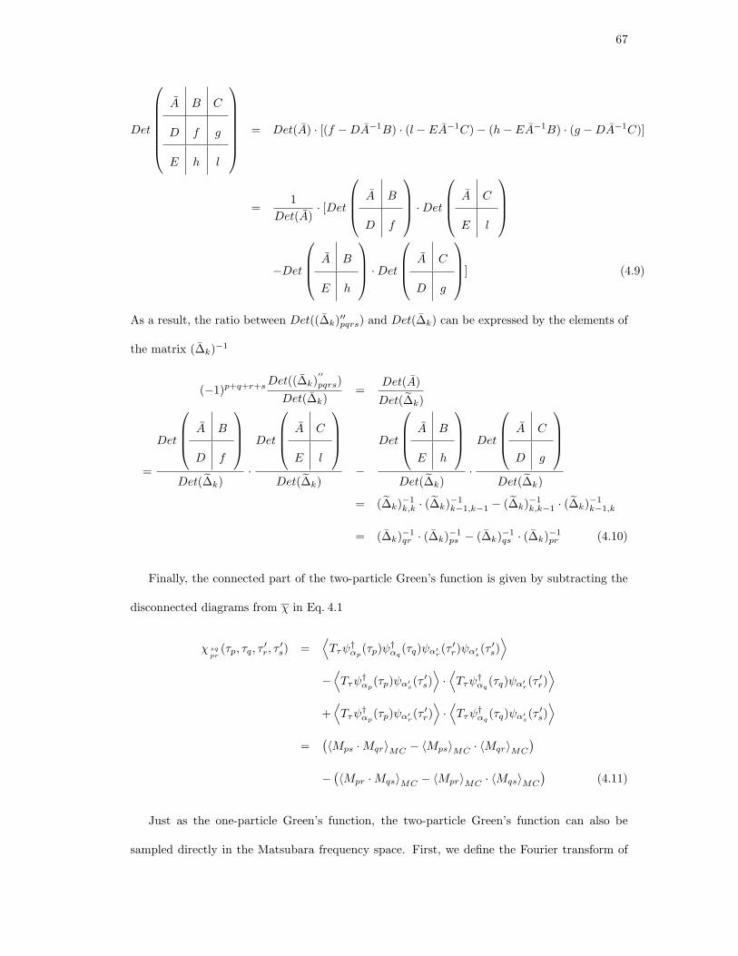
67

Det

A B C

D f g

E h l

= Det(A) · [(f − DA−1B) · (l − EA−1C) − (h − EA−1B) · (g − DA−1C)]

=1

Det(A)· [Det

A B

D f

· Det

A C

E l

−Det

A B

E h

· Det

A C

D g

] (4.9)

As a result, the ratio between Det((∆k)′′pqrs) and Det(∆k) can be expressed by the elements of

the matrix (∆k)−1

(−1)p+q+r+sDet((∆k)

′′

pqrs)

Det(∆k)=

Det(A)

Det(∆k)

=

Det

A B

D f

Det(∆k)·

Det

A C

E l

Det(∆k)−

Det

A B

E h

Det(∆k)·

Det

A C

D g

Det(∆k)

= (∆k)−1k,k · (∆k)−1

k−1,k−1 − (∆k)−1k,k−1 · (∆k)−1

k−1,k

= (∆k)−1qr · (∆k)−1

ps − (∆k)−1qs · (∆k)−1

pr (4.10)

Finally, the connected part of the two-particle Green’s function is given by subtracting the

disconnected diagrams from χ in Eq. 4.1

χ sqpr

(τp, τq, τ′r, τ

′s) =

⟨Tτψ†

αp(τp)ψ

†αq

(τq)ψα′r(τ ′

r)ψα′s(τ ′

s)⟩

−⟨Tτψ†

αp(τp)ψα′

s(τ ′

s)⟩·⟨Tτψ†

αq(τq)ψα′

r(τ ′

r)⟩

+⟨Tτψ†

αp(τp)ψα′

r(τ ′

r)⟩·⟨Tτψ†

αq(τq)ψα′

s(τ ′

s)⟩

=(〈Mps · Mqr〉MC − 〈Mps〉MC · 〈Mqr〉MC

)

−(〈Mpr · Mqs〉MC − 〈Mpr〉MC · 〈Mqs〉MC

)(4.11)

Just as the one-particle Green’s function, the two-particle Green’s function can also be

sampled directly in the Matsubara frequency space. First, we define the Fourier transform of

68

the matrix Mij(τi, τj)

Mij(iν1, iν2) =1

β

∑

τi,τ ′j

ei(ν1τi−ν2τ ′j)Mij(τi, τ

′j) (4.12)

Due to the time translation invariance, the two-particle Green’s function depends on the three

Matsubara frequencies (iν,iν′, and iω)

χ sqpr

(iν, iν′)iω =1

β2

∫ β

0

dτp

∫ β

0

dτq

∫ β

0

dτ ′r

∫ β

0

dτ ′se

i(ντp+(ν′+ω)τq−ν′τ ′r−(ν+ω)τ ′

s)χ sqpr

(τp, τq, τ′r, τ

′s)

= [〈Mps(iν, iν + iω) · Mqr(iν′ + iω, iν′)〉MC

−〈Mps(iν, iν + iω)〉MC · 〈Mqr(iν′ + iω, iν′)〉MC ]

−[〈Mpr(iν, iν′) · Mqs(iν′ + iω, iν + iω)〉MC

−〈Mpr(iν, iν′)〉MC · 〈Mqs(iν′ + iω, iν + iω)〉MC ] (4.13)

This is the full and connected two-particle Green’s function of the impurity problem, which

sampled by the Monte Carlo method. It is the central quantity of the vertex function approach,

from which the local two-particle irreducible vertex is obtained. In later sections, we will

discuss how to compute the magnetic/charge susceptibility and the superconducting pairing

susceptibility using this sampled vertex function.

4.3 The high frequency asymptotics of the two-particle Green’s func-

tion

The two-particle Green’s function χ αδβγ

(iν, iν′)iω sampled by CTQMC is stored as a N × N

complex matrix where N is nν × n2b × n2

s and nν is the number of Matsubara frequencies, nb is

the number of orbitals, and ns is 2. Here, the range of iν and iν′ is restricted to the low energy

region since χ falls off with the frequency as 1ν2 and the sampled Monte Carlo data contain a

lot of noise at high frequencies. The one-particle Green’s function or the self energy also has

noise at the high frequencies, but it is replaced by the analytic formula given as a function of

lattice parameters such as the bare interaction U and the electron density n.

For the two-particle quantities, the approximate formula for the high frequency asymptotics

69

of the irreducible vertex function Γirr was derived in Ref. [78]. The Monte Carlo method can

sample χ without severe noise only at the restricted low frequency region while this analytic

expression for Γirr is valid only in the high frequency region. The Bethe-Salpeter equation (refer

to Eq. 4.27) which relates Γirr and χ is a matrix equation in the frequency space, therefore,

low frequency values and high frequency values are mixed and it is not sufficient to have one

quantity only at high frequency and different quantity at low frequency. Ref. [78] uses the

blocked Bethe-Salpeter equation to resolve this problem.

Here, we propose a high frequency extrapolation method for χ employing the singular

value decomposition (SVD) for the χ αδβγ

(iν, iν′)iω matrix. For each spin and orbital compo-

nent α, β, γ, δ and at fixed center of mass frequency iω, we decompose χ(iν, iν′) matrix by SVD

method

χ(iν, iν′) =∑

k

φLk (iν) · λk · φR

k (iν′) (4.14)

where λk is the k-th singular value and φL/Rk is the corresponding left/right singular vector. The

range of iν and iν′ is limited to within the sampled range, i.e., −νc ≤ ν ≤ νc and −νc ≤ ν′ ≤ νc.

Generally, the high frequency asymptotics of χ is not analytically known function since the

Bethe-Salpeter equation mixes up the low frequency part and the high frequency part. The

advantage of the SVD form is that the mixture of the low frequency and the high frequency is

effectively decoupled and it is sufficient to extrapolate the high frequency part of the singular

vectors. One should note that at the high frequency region where only one frequency iν goes

to infinity, the low frequency values of φk(iν′) also contribute to the asymptotics. Our simu-

lation shows that the high frequency behavior of the singular vector φL/Rk in Eq. 4.14 can be

extrapolated using the sampled values of φL/Rk . In the limit of iν → ∞ with the fixed iν′ and

iω, the high frequency behavior of χ is proportional to the polarization function χ0 since the

full vertex Γ(iν → ∞, iν′)iω is asymptotically approaching a constant at high frequency.

The two-particle Green’s function χ consists of the full vertex function and the four external

70

legs

χ(iν, iν′) = g(iν) · g(iν + iω) · Γ(iν, iν′) · g(iν′ + iω) · g(iν′) (4.15)

The local Green’s function g is diagonal in the spin and the orbital space at high frequencies

and Γ is the full vertex function. As a result, the asymptotic behavior of χ at iν → ∞ and the

finite iν′ is given by

χ(iν → ∞, iν′) ∝ g(iν) · g(iν + iω) (4.16)

Similar relation is also valid for χ(iν, iν′ → ∞). Using this asymptotic behavior, the singular

vectors of Eq. 4.14 at high frequency region are given by

φL(R)k (iν → ∞) ∼= c

L(R)k · g(iν) · g(iν + iω) (4.17)

Singular vectors contain substantial amount of noise at high frequency, hence we need to

carefully extract the coefficients cL(R)k from the numerically sampled data. We use the following

approximation

cL(R)k =

1

Nν

iνc∑

iν=iνs

(φ

L(R)k (iν)

g(iν) · g(iν + iω)

)(4.18)

where iν runs over last few Matsubara points Here, iν values range from iνs to iνc and Nν is

the number of Matsubara points for the average. The resulting singular vector, valid at both

high and low frequency is thus obtained by

φL(R)k (iν) =

φL(R)k (iν) if |ν| ≤ |νc|

cL(R)k · gα(δ)(iν) · gβ(γ)(iν + iω) if |ν| ≥ |νc|

(4.19)

Finally, the high frequency approximation for the two-particle Green’s function χ is con-

structed by

χ(iν, iν′)iω =∑

k<kc

φLk (iν) · λk · φR

k (iν′) (4.20)

where k runs over a few largest singular values. Singular vectors that correspond to small

singular values contain increasingly severe noise. As we will show below, the irreducible vertex

71

is computed by inverting χ, therefore, the noise from small singular values can severely impact

the quality of the irreducible vertex. Therefore, we keep only the large singular values (k < kc)

for constructing the high frequency tails of χ. For the low frequency values, the χ already

sampled from CTQMC is still used.

χ(iν, iν′) =

χ(iν, iν′) if |ν| ∧ |ν′| ≤ νc

χ(iν, iν′) if |ν| ∨ |ν′| ≥ νc

(4.21)

We believe that our method to determine the asymptotic behavior of χ is very efficient

provided that the reliable data for χ at reasonable range of frequencies iν and iν′ is available.

More importantly, our method is also applicable to the general multi-orbital situation.

4.4 Calculation of the magnetic and the charge susceptibility

iν + iω, α3α′3

iν, α′1α1

iν′ + iω, α′4α4

iν′, α2α′2

iν + iω, α3α4

iν, α2α1

iν + iω, α3α′3

iν, α′1α1

iν′ + iω, α′4α4

iν′, α2α′2

Γirrloc χm(d)χm(d) χ0 χ0+=

Figure 4.2: The Feynman diagram for the Bethe-Salpeter equation in the spin (charge) channel.The non-local susceptibility is obtained by replacing the local propagator by the non-localpropagator.

In this section, we explain how to compute the magnetic and the charge susceptibility

χ(m/d)(q, iω) from the ab initio perspective within the DFT+DMFT method. First, the

local (impurity) Green’s function is computed for the correlated orbitals as a result of the

DFT+DMFT self-consistent loop. The local (impurity) polarization bubble χ0(iν)iω is com-

puted from this fully interacting one-particle Green’s function by

χ0loc, α1σ1,α2σ2

α3σ3,α4σ4

(iν, iν′)iω = −T · Gα2α1,σ1(iν) · Gα3α4,σ3

(iν + iω) · δiν,iν′ · δσ1σ2· δσ3σ4

(4.22)

Here, σ1−4 are the spin indices and α1−4 are the orbital indices which run over correlated orbital

states on the atom. And T is the temperature. The Green’s function is diagonal in the spin

72

and the Matsubara frequency space due to the spin conservation and the time translational

invariance. However, it is generally off-diagonal in the orbital space since the different orbital

characters can mix at a generic momentum point For solids with high symmetry of the lattice,

the local propagator is diagonal in orbital space when expressed in the crystral field harmonics.

The local two-particle Green’s function χsampleloc is sampled by CTQMC using the converged

DFT+DMFT solution. The procedure of sampling χsampleloc is explained in detail in section. 4.2.

CTQMC samples only the connected diagrams of χloc, i.e., the rightmost diagram of Fig. 4.2.

The full χloc is obtained by adding the local polarization bubble to the sampled diagram.

χloc, α1σ1,α2σ2α3σ3,α4σ4

(iν, iν′)iω = [χ0loc + χsample

loc ]α1σ1,α2σ2α3σ3,α4σ4

(iν, iν′)iω (4.23)

The matrix size of χloc at a fixed iω is given as N ×N where N is (the number of spins)2×(the

number of orbitals)2×(the number of Matsubara frequencies iν). Due to the large matrix size,

it is desirable to use spin symmetry to reduce the matrix size. Under the spin rotation, the two-

particle response functions in the particle-hole channel can be decomposed into the magnetic

(m) channel and the density (d) channel as follows:

χm(d)

loc, α1,α2α3,α4

(iν, iν′)iω = χloc, α1↑,α2↑

α3↑,α4↑

(iν, iν′)iω − (+)χloc, α1↑,α2↓

α3↑,α4↓

(iν, iν′)iω (4.24)

The two-particle irreducible vertex function Γirrloc is the vertex function which can not be

separated into two parts by cutting two propagators. Γirrloc is assumed to be local in the same

basis in which the DMFT self-energy is local. In order to extract Γirrloc , we employ the Bethe-

Salpeter equation (see Fig. 4.2) which relates the local two-particle Green’s function (χloc)

sampled by CTQMC, with both the local polarization function (χ0loc) and Γirr

loc .

Γirr,m(d)

loc α1,α2α3,α4

(iν, iν′)iω = [(χ0loc)

−1iω − χ

m(d)−1loc ]α1,α2

α3,α4(iν, iν′)iω. (4.25)

Γirrloc also depends on three Matsubara frequencies (iν, iν′; iω) just as χloc.

Once the irreducible vertex Γirrloc is obtained, the momentum dependent two-particle Green’s

function is constructed using again the Bethe-Salpeter equation (Fig. 4.2) by replacing the local

polarization function χ0loc by the non-local one χ0

q,iω. Since Γirrloc is local, we can sum over the

73

momentum k inside the non-local polarization bubble

χ0α1σ1,α2σ2α3σ3,α4σ4

(iν, iν′)q,iω = − T

Nk

∑

k

Gα2α1,σ1(k, iν) · Gα3α4,σ3

(k + q, iν + iω) · δiν,iν′ · δσ1σ2· δσ3σ4

(4.26)

to bring the Bethe-Salpeter equation into a simplified form

χm(d)α1,α2α3,α4

(iν, iν′)q,iω = [(χ0)−1q,iω − Γ

irr,m(d)loc ]−1

α1,α2α3,α4

(iν, iν′)q,iω. (4.27)

Finally, the spin and charge susceptibility χm(d)(q, iω) is obtained by closing the two particle

Green’s function with spin or charge bare vertex γ (γ is 1/2 for spin and γ is 1 for charge) and

summing over frequencies (iν,iν′) and orbitals (α1,2) on the four external legs

χm(d)(q, iω) = 2γ2∑

iν,iν′

∑

α1α2

χm(d)α1,α2α1,α2

(iν, iν′)q,iω. (4.28)

The algorithm for computing the magnetic and the charge susceptibility is sketched in Fig.4.3

4.5 The calculation of the superconducting pairing susceptibility

4.5.1 The irreducible vertex function in the particle-particle channel

Γirr,p−p

The two-particle vertex functions depend on four spin σ1−4 and four orbital α1−4 indices, and

three Matsubara frequencies (iν,iν′, and iω) and momentums (k,k′, and q) which are labeled

on the external legs.

Depending on the nature of the quasi-particle scattering, the two-particle vertex function

can be expressed in terms of two distinct types of diagrams, so called channels. They are the

particle-hole and the particle-particle channels. A representative of the particle-particle and the

particle-hole channel is depicted in Fig. 4.4(a).

As already discussed in the previous section, the spin degrees of freedom in the particle-hole

channel can be decomposed into either magnetic (m) channel or charge (d) channel distin-

guished by the different spin eigenstates if the spin-orbit coupling is small. The magnetic

74

CTQMC

Sample Gloc(i) and loχ(i,i)i

Compute 0loχ(i)iCompute irr,m(d)

loχ(i,i)i

Compute 0 (i)q,iCompute the full m(d) (q,i) from B.S.E

change ichange q

Figure 4.3: The flow chart for computing the magnetic and the charge susceptibility

75

k, iν, α1 σ1

k′, iν′, α2 σ2

σ3 − k + q,−iν + iω, α3

σ4 − k′ + q,−iν′ + iω, α4

k, iν, α1 σ1

k + q, iν + iω, α2 σ2

σ3 k′, iν′, α3

σ4 k′ + q, iν′ + iω, α4

(a)Γp−p

≡ Γp−pα2σ2,α4σ4α1σ1α3σ3

(k, iν,k′, iν ′)q,iω Γp−h

≡ Γp−hα2σ2,α4σ4α1σ1,α3σ3

(k, iν,k′, iν ′)q,iω

↑ kα1

↑ k′

α2

−k ↓α3

−k′ ↓α4

↑ iνα1

↑ iν′

α2

−iν ↓α3

−iν′ ↓α4

↑ iν, α1

α4,−iν′ ↓↑ iν′, α2

α3,−iν ↓

↑ iν, α1

↑ iν′, α2 α4,−iν′ ↓

α3,−iν ↓

Γirrp−p Γf.irr Γirr

p−h χp−h

k′−k Γirr

p−h

Γirrp−h χ

p−h

k′+k

Γirrp−h

−

+

=(b)

Figure 4.4: (a) The spin, orbital, momentum, and frequency labels of vertex functions in theparticle-particle (p − p) channel and the particle-hole (p − h) channel. (b) The decompositionof the irreducible vertex function in the particle-particle channel Γirr,p−p.

76

channel contains either the longitudinal spin configuration (denoted as p − h1) or the trans-

verse configuration (denoted as p − h2). In the magnetic susceptibility, the paramagnetic spin

rotational symmetry ensures that 2〈Sz · Sz〉 = 12 (〈S+ · S−〉 + 〈S− · S+〉) where S is the spin

operator. Here, 〈Sz · Sz〉 represents the longitudinal susceptibility while 〈S+ · S−〉 indicates the

transverse term. As a result, one can express the vertex function in the magnetic channel with

explicit spin indices (↑, ↓) as a function of p − h1 and p − h2 channels.

Γp−h,(m) = Γp−h1↑↑↑↑

− Γp−h1↑↓↑↓

= Γp−h2↓↓↑↑

(4.29)

In a similar way, the charge channel also can be represented in both p−h1 and p−h2 channels.

Γp−h,(d) = Γp−h1↑↑↑↑

+ Γp−h1↑↓↑↓

= 2Γp−h2↑↑↑↑

− Γp−h2↓↓↑↑

(4.30)

The last equality is derived using Γp−h1↑↑↑↑

= Γp−h2↑↑↑↑

.

The particle-particle channel describes the Cooper pairing for superconductivity. And this

channel also can be decomposed according to spin configurations into the singlet (s) channel

and the triplet (t) channel. The singlet channel has the odd symmetry under the exchange of

two external spins while the triplet channel has the even symmetry.

Γp−p,(s) =1

2[Γp−p

↑↓↑↓

− Γp−p↓↑↑↓

] (4.31)

Γp−p,(t) =1

2[Γp−p

↑↓↑↓

+ Γp−p↓↑↑↓

] (4.32)

From now on, we concentrate on superconductivity in the singlet channel. In this case, the

Cooper pair has the odd symmetry under the spin exchange. One can note that the vertex

function in the particle-particle channel Γp−p acquires a minus sign by crossing the two outgoing

legs due to the exchange of two fermion operators. Since the vertex Γp−p is odd under the

exchange of spin in the singlet channel, Γp−p has to be even under the exchange of momentum,

orbital, and frequency.

Here, we introduce several kinds of vertex functions which we will use later. We first con-

centrate on the particle-hole channel. The connected two-particle Green’s function χ matrix

defined as

χ 2,41,3

= 〈ψ†1ψ

†4ψ3ψ2〉 − 〈ψ†

1ψ2〉 · 〈ψ†4ψ3〉 + 〈ψ†

1ψ3〉 · 〈ψ†4ψ2〉 (4.33)

77

is related to the polarization bubble χ0 and the irreducible vertex Γirr by the Bethe-Salpeter

equation

χ = χ0 + χ = [(χ0)−1 − Γirr]−1. (4.34)

χ = [(χ0)−1 − Γirr]−1 − χ0 = [(χ0 · Γirr · χ0)−1 − (χ0)−1]−1. (4.35)

Here, χ0 is given by −T · G · G. We omit spin, orbital, momentum, and frequency labels for

convenience.

The two-particle full vertex function Γfull is defined as all connected diagrams obtained by

removing two external polarization bubbles from χ

Γfull = (χ0)−1 · χ · (χ0)−1

= [(Γirr)−1 − χ0]−1

= Γirr + Γirr · χ0 · Γirr + Γirr · χ0 · Γirr · χ0 · Γirr + · · · (4.36)

As a result, Γfull is given by dressing Γirr with χ0.

In contrast to Γirr, the reducible vertex function Γ is defined as the vertex function which

can be separated into two parts by cutting two propagators. Γ is obtained by subtracting the

irreducible part from Γfull.

Γ = Γfull − Γirr

= Γirr · χ0 · Γirr + Γirr · χ0 · Γirr · χ0 · Γirr + · · ·

= Γirr · χ · Γirr (4.37)

Considering both particle-hole and particle-particle channels, we can define the vertex which

is irreducible with respect to all channels. The fully irreducible vertex Γf.irr consists of diagrams

which can not be separated into two parts by cutting any two propagators, either particle-

particle or particle-hole pair of propagators.

The irreducible vertex function in the particle-particle channel Γirr,p−p, which gives the

pairing interaction for Cooper pairs, consists of the fully irreducible vertex function Γf.irr and

the reducible vertex functions in the other particle-hole channels Γp−h = Γfull,p−h − Γirr,p−h.

78

We keep track of the spin, orbital, and frequency labels as shown in Fig. 4.4. Note that we plot

Γ in the expanded form Γirr · χ · Γirr in Fig. 4.4(b). Moreover, we concentrate on uniform and

static superconductivity, i.e. q = 0, iω = 0,

Γirr,p−pα2↑,α4↓

α1↑,α3↓

(k, k′)q=0 = Γf−irrα2↑,α4↓

α1↑,α3↓

(k, k′)q=0 − Γp−h1α2↑,α3↓

α1↑,α4↓

(k,−k′)k′−k + Γp−h2α4↓,α3↓

α1↑,α2↑

(k, k′)−k′−k (4.38)

Here, the label k = (k, iν) represents both momentum and frequency.

Γirr,p−p in the spin singlet state, which is denoted by Γirr,p−p,(s), is obtained by antisym-

metrizing the spin space as in Eq. 4.31. One spin configuration for Eq. 4.31 is given in Eq. 4.38

and depicted in Fig. 4.4(b). The other spin configuration can be obtained in a similar way as

Γirr,p−pα2↓,α4↑

α1↑,α3↓

(k, k′)q=0 = Γf−irrα2↓,α4↑

α1↑,α3↓

(k, k′)q=0 − Γp−h2α2↓,α3↓

α1↑,α4↑

(k,−k′)k′−k + Γp−h1α4↑,α3↓

α1↑,α2↓

(k, k′)−k′−k (4.39)

Due to the exchange of the spin label, p − h1 and p − h2 channels are also exchanged. Using

Eq. 4.29 and Eq. 4.30, p − h1 and p − h2 channels can be represented as the magnetic/charge

channel

Γp−h1↑↓↑↓

=1

2[Γp−h,(d) − Γp−h,(m)] (4.40)

Γp−h2↓↓↑↑

= Γp−h,(m) (4.41)

Γirr,p−p in Eq. 4.38 and Eq. 4.39 also can be represented as the magnetic/charge channel

Γirr,p−pα2↑,α4↓

α1↑,α3↓

(k, k′)q=0 = Γf−irrα2↑,α4↓

α1↑,α3↓

(k, k′)q=0−1

2[Γp−h,(d)−Γp−h,(m)]α2,α3

α1,α4(k,−k′)k′−k+Γ

p−h,(m)α4,α3α1,α2

(k, k′)−k′−k

(4.42)

Γirr,p−pα2↓,α4↑

α1↑,α3↓

(k, k′)q=0 = Γf−irrα2↓,α4↑

α1↑,α3↓

(k, k′)q=0−Γp−h,(m)α2,α3α1,α4

(k,−k′)k′−k+1

2[Γp−h,(d)−Γp−h,(m)]α4,α3

α1,α2(k, k′)−k′−k

(4.43)

Finally Γirr,p−p,(s) is obtained using Eq. 4.31 as

Γirr,p−p,(s)α2,α4α1,α3

(k, k′)q=0 = Γf−irr,(s)α2,α4α1,α3

(k, k′)q=0 +1

2[3

2Γp−h,(m) − 1

2Γp−h,(d)]α2,α3

α1,α4(k,−k′)k′−k

+1

2[3

2Γp−h,(m) − 1

2Γp−h,(d)]α4,α3

α1,α2(k, k′)−k′−k (4.44)

One can note that the reducible vertex [32 Γp−h,(m) − 12 Γp−h,(d)] is symmetrized under the ex-

change of orbitals (α2 ↔ α4), momentum, and frequency (k′ ↔ −k′).

79

It is well known from BCS theory that the attractive pairing vertex in the s-wave symmetry

channel can mediate the pairing interaction for Cooper pairs. The pairing vertex given in

Eq. 4.44 is constructed from the Coulomb interaction vertex and the vertex has the repulsive

nature in the average. Therefore, the pairing susceptibility calculated using this repulsive vertex

can not develop a pole in the s-wave channel and s-wave superconductivity is excluded among

the possible pairing channels.

Although the pairing vertex in Eq. 4.44 is repulsive in the s-wave channel, the momentum

dependent pairing vertex can be effectively attractive in higher angular momentum channels

such as d-wave or extended s-wave. Indeed, this non-local symmetry is realized in many high

Tc superconductors where the pairing is believed to be mediated by spin fluctuations.

In order to evaluate the non-local pairing vertex Γirr,p−p,(s), we resort here to the DMFT

approximation. In this approximation, we assume that the fully irreducible vertex Γf.irr is lo-

cal and the irreducible vertices in the particle-hole channels (Γirr,(m),Γirr,(d)) are local as well.

These irreducible vertices can be computed from the corresponding impurity quantities. On the

other hand, the irreducible vertex in the particle-particle channel is not local but will be com-

puted from the particle-hole diagrams as depicted in Fig.4.4(b). Explicitly, the magnetic/charge

susceptibility are obtained by the Bethe-Salpeter equation

χp−h,(m/d)α2,α4α1,α3

(iν1, iν2)q,iω = [(χp−h0 )−1

q,iω − Γirr,p−h,(m/d)loc ]α2,α4

α1,α3(iν1, iν2)q,iω (4.45)

and the reducible magnetic/charge vertex is obtained from this non-local magnetic/charge sus-

ceptibility by

Γp−h,(m/d)α2,α4α1,α3

(iν, iν′)q,iω =∑

iν1,iν2

∑

α′2,α′

4α′1,α′

3

Γirr,p−h,(m/d)

loc,α2,α′

2α1,α′

1

(iν, iν1)iω · χp−h,(m/d)α′2,α′

4α′1,α′

3

(iν1, iν2)q,iω

·Γirr,p−h,(m/d)α′4,α4

α′3,α3

(iν2, iν′)iω (4.46)

Here, the non-local polarization is χ0,p−h(iν)q,iω = − TNk

∑k G(k, iν) · G(k + q, iν + iω) and

the non-local Green’s function G(k, iν) is dressed with the local DMFT self-energy. Note

that Eq. 4.45 was used before in the previous section (Eq. 4.27) to compute the non-local

magnetic/charge susceptibility.

80

Finally, the non-local pairing vertex is obtained from the particle-hole reducible vertices by

Γirr,p−p,(s)α2,α4α1,α3

(k, iν,k′, iν′) = Γf−irr,(s)α2,α4α1,α3

(iν, iν′) + [3

2Γp−h,(m) − 1

2Γp−h,(d)]α2,α3

α1,α4(iν,−iν′)k′−k,iν′−iν

+1

2[3

2Γp−h,(m) − 1

2Γp−h,(d)]α4,α3

α1,α2(iν, iν′)−k′−k,−iν′−iν (4.47)

In practice, one can compute the only one term of [32 Γp−h,(m) − 12 Γp−h,(d)] and symmetrize the

result with respect to orbitals (α2 ↔ α4), momentum (k′ ↔ −k′), and frequency (iν′ ↔ −iν′).

Within our DMFT approximation, Γf−irr is assumed to be purely local. Indeed, Ref. [71]

confirms the weak momentum dependence of Γf−irr vertex within cluster DMFT. Since Γf−irr is

local, it could be in principle computed from the corresponding impurity vertex. In the following,

we concentrate on the non-local pairing symmetry, such as d-wave, p-wave, or extended s-wave.

In these cases, the local Γf−irr does not contribute to the non-local pairing gap symmetry.

4.5.2 The calculation of the superconducting critical temperature and

the gap symmetry

In the previous subsection, the non-local irreducible vertex function in the particle-particle

channel Γirr,p−p is computed using DMFT vertex functions. The Γirr,p−p vertex accounts

for the pairing interaction of Cooper pairs and as a result the superconducting instability.

Eq. 4.47 shows that this pairing vertex contains the spin fluctuation diagrams and the orbital

(charge) fluctuation diagrams. In general, the spin fluctuation contribution is much larger near

a magnetic phase transition.

The pairing susceptibility χp−p is computed by dressing the pairing polarization bubble

χ0,p−p(k, iν) with the pairing vertex Γirr,p−p,(s) using the Bethe-Salpeter equation in the particle-

particle channel.

χp−p = χ0,p−p − χ0,p−p · Γirr,p−p,(s) · χ0,p−p

+χ0,p−p · Γirr,p−p,(s) · χ0,p−p · Γirr,p−p,(s) · χ0,p−p − · · ·

= χ0,p−p · [1 + Γirr,p−p,(s) · χ0,p−p]−1 (4.48)

81

The critical temperature Tc of the superconducting state is determined as the temperature

where this pairing susceptibility diverges. The sufficient condition for the divergence is at least

one eigenvalue of the pairing matrix −Γirr,p−p,(s) · χ0,p−p reaches one. Therefore, Tc can be

computed by solving the following eigenvalue equation without the need to compute the full

pairing susceptibility.

− T

Nk

∑

k′,iν′

∑

α2,α4α5,α6

Γirr,p−p,(s)α2,α4α1,α3

(k, iν,k′, iν′) ·χ0,p−pα5,α6α2,α4

(k′, iν′) ·φλα5α6

(k′, iν′) = λ ·φλα1α3

(k, iν) (4.49)

Here, λ is the eigenvalue of the pairing kernel matrix and Tc is determined as the temperature

at which the leading eigenvalue approaches unity. The corresponding eigenvector φλ gives the

pairing symmetry in momentum and orbital space of the superconducting state which will be

stable below Tc. Not just momentum but also the orbital contribution to the gap symmetry

might play an important role in the Fe-based superconductors due to their multi-orbital nature.

The pairing bubble diagram χ0,p−p is computed as a product of DMFT Green’s functions.

This Green’s function is dressed with the local DMFT self energy.

χ0,p−pα2,α4α1,α3

(k, iν)q=0,iω=0 = T · Gα1α2,↑(k, iν) · Gα3α4,↓(−k,−iν) (4.50)

One can note that the polarization bubble in the particle-particle channel (χ0,p−p) has no

minus sign while the particle-hole polarization bubble χ0,p−h has it due to the closed loop of

the diagram. As will be shown in the next chapter, this pairing bubble χ0,p−p can incorporate

the non-local fluctuation effect beyond DMFT replacing the DMFT Green’s function by the

Green’s function computed with non-local methods.

The eigenvalue problem in Eq. 4.49 involves the diagonalization of a non-Hermitian matrix

of size Nν × Nk × N2orb where Nν is the number of frequency, Nk is the number of k points,

and Norb is the number of orbitals. The spin degree of freedom is projected to the singlet state.

For reliable results, we need at least 20 frequency points and 1000 k points in the Brillouin

zone. For the multi-orbital case with five relevant d orbitals, the matrix size can be larger than

500,000. Therefore, it is desirable to transform this matrix into a Hermitian form for which

there exists very efficient algorithms such as the Lanczos method to obtain the largest eigenvalue

82

and eigenfunction. The original χp−p given in Eq. 4.48 can be expressed in a symmetric way

χp−p = χ0,p−p · [1 + Γirr,p−p,(s) · χ0,p−p]−1

=√

χ0,p−p ·√

χ0,p−p · [1 + Γirr,p−p,(s) · χ0,p−p]−1 · (√

χ0,p−p)−1 ·√

χ0,p−p

=√

χ0,p−p · [1 +√

χ0,p−p · Γirr,p−p,(s) ·√

χ0,p−p]−1 ·√

χ0,p−p (4.51)

As a result, the gap function in Eq. 4.49 can be brought to a Hermitian form by

− T

Nk

∑

k′,iν

∑

α2α4α5α6α7α8

√χ0,p−p

α2,α4α1,α3

(k, iν)·Γirr,p−p,(s)α5,α7α2,α4

(k, iν,k′, iν′)·√

χ0,p−pα6,α8α5,α7

(k′, iν′)·φλα6α8

(k′, iν′) = λ·φλα1α3

(k, iν)

(4.52)

One can note that√

χ0,p−p · Γirr,p−p,(s) ·√

χ0,p−p matrix is a Hermitian matrix (in single

orbital case it is also real). Therefore, we use the Lanczos algorithm to compute the leading

and the subleading eigenvalues and the corresponding eigenfunctions.

The eigenfunction computed using the non-Hermitian gap equation in Eq. 4.49 is related to

the eigenfunction φλ in Eq. 4.52.

√χ0,p−p · Γirr,p−p,(s) ·

√χ0,p−p · φλ = λ · φλ (4.53)

Γirr,p−p,(s) · χ0,p−p((√

χ0,p−p)−1 · φλ) = λ · ((√

χ0,p−p)−1 · φλ) (4.54)

This equation shows that eigenvalues of the non-Hermitian gap equation (Eq.4.49) are the same

as eigenvalues of the Hermitian gap equation (Eq. 4.52). And the right eigenvector of Eq. 4.49

is given as (√

χ0,p−p)−1 · φλ where φλ is the eigenvector of Eq. 4.52. In a similar way, the left

eigenvector is given as√

χ0,p−p · φλ

The pairing susceptibility χp−p can be represented as a function of eigenvalues λ and eigen-

functions φλ of the Hermitian pairing matrix (Eq. 4.52) using the eigendecomposition of the

matrix.

χp−p(k, k′) =√

χ0,p−p(k) · [1 +√

χ0,p−p · Γirr,p−p,(s) ·√

χ0,p−p]−1 ·√

χ0,p−p(k′)

=√

χ0,p−p(k) · [U · U† − U · Λ · U†]−1 ·√

χ0,p−p(k′)

=√

χ0,p−p(k) · U · [1 − Λ]−1 · U† ·√

χ0,p−p(k′)

=∑

λ

1

1 − λ· (

√χ0,p−p(k) · φλ(k)) · (

√χ0,p−p(k′) · φλ(k′)) (4.55)

83

where Λ is the diagonal matrix whose i-th diagonal element is the i-th eigenvalue λi of the

Hermitian pairing matrix and U is the unitary matrix whose columns are the corresponding

eigenvectors. It is obvious that the pairing susceptibility diverges when the leading eigenvalue

obtained from Eq. 4.52 approaches one. The corresponding eigenfunction represents the mo-

mentum structure of χp−p, i.e., the gap symmetry of the SC state.

The overall procedure for computing the pairing susceptibility is depicted in Fig. 4.5.

CTQMC

Sample Gloc(i) and loχ(i,i)iCompute irr,m(d)

loχ(i,i)i

Compute 0 (i)q,i and m(d) (i,i)q,iCompute ph,m(d)

(i,i)q,iCompute irr,pp (k,i,k,i)

and symmetize it

Compute the leading and using Lanczos algorithm

change ichange q

Figure 4.5: The flow chart for computing the pairing susceptibility

84

4.5.3 Relevant quantities for superconductivity

The projected pairing interaction

The pairing vertices Γirr,p−p,(s) projected to different symmetry channels are denoted by Γ(α),p−p

and can be computed by

Γ(α),p−pα2,α4α1,α3

=

∑k,k′ g(α)(k) · Γirr,p−p,(s)

α2,α4α1,α3

(k, πT,k′, πT ) · g(α)(k′)

∑k

(g(α)(k)

)2 (4.56)

Here, g(α)(k) represents different pairing channels, for example, g(α)(k) = (cos(kx) − cos(ky))

for the d-wave and g(α)(k) = (cos(kx)+cos(ky)) for the extended s-wave. Since Γirr,p−p,(s) falls

off rapidly with frequency, the pairing vertex value for the lowest Matsubara point is considered

similar as in Ref. [79]. This pairing interaction is repulsive in the s-wave channel but it can be

attractive in other symmetry channels.

The projected pairing bubble

The pairing bubble summed over the Matsubara frequencies χ0,p−p also can be projected to

different symmetry channels in a similar way as in Eq. 4.56.

χ0,p−pα2,α4α1,α3

=T

∑k,iν g(k) · χ0,p−p

α2,α4α1,α3

(k, iν) · g(k)∑

k (g(k))2 (4.57)

The effective U

As discussed in subsection 4.5.1, the spin-fermion interaction vertex within DMFT is given by

the local irreducible vertex in the particle-hole channel Γirr,p−h. In the case of weak interactions,

this irreducible vertex function is usually approximated by the bare interaction or the effectively

screened interaction U which is independent of frequency but still retains the spin and the

orbital dependence. This is the so called random phase approximation (RPA). Within this

85

approximation, the reducible particle-hole vertex in Eq. 4.47 is simplified to

Γirr,p−pα2,α4α1,α3

(k, iν,k′, iν′) =3

2

∑

α′2,α′

4α′1,α′

3

U(m)α2,α′

2α1,α′

1

· χp−h,(m)α′2,α′

4α′1,α′

3,k′−k,iν′−iν

· U (m)α′4,α4

α′3,α3

−1

2

∑

α′2,α′

4α′1,α′

3

U(d)α2,α′

2α1,α′

1

· χp−h,(d)α′2,α′

4α′1,α′

3,k′−k,iν′−iν

· U (d)α′4,α4

α′3,α3

(4.58)

Here, U(m/d)α2,α4α1,α3

are the bare interaction with the orbital dependence in the magnetic and the den-

sity channel and χp−h,(m/d)α2,α4α1,α3

is the RPA magnetic or charge susceptibility. This bare interaction

matrix includes the intra-(inter-) orbital interaction term, the Hund’s coupling term, and the

pair-hopping term [80, 81].

In the vertex calculation, the spin-fermion interaction vertex depends on frequencies given

as Γirr,p−h. The effective spin-fermion vertex U within DMFT can be determined by equating

the Γirr,p−p vertex at the lowest Matsubara point in Eq. 4.47 with the RPA form in Eq. 4.58

Γp−h,(m/d)α2,α4α1,α3

(πT, πT )q,iω=0 =∑

α′2,α′

4α′1,α′

3

U(m/d)α2,α′

2α1,α′

1,q· χp−h,(m/d)

α′2,α′

4α′1,α′

3,q,iω=0

· U (m/d)α′4,α4

α′3,α3

,q(4.59)

Here, U is evaluated only at iω=0 assuming the iω dependence of U is weak. The Γp−h,(m/d)

vertex at higher iω values can be computed more efficiently from the RPA form in Eq. 4.59

using the computed U at iω=0. In the single orbital case, U(m/d)

q is given as

U(m/d)

q =

√[Γirr,p−h,(m/d) · χp−h(m/d) · Γirr,p−h,(m/d)](πT, πT )q,iω=0∑

iν,iν′ χp−h,(m/d)(iν, iν′)q,iω=0(4.60)

The effective Uq is now slightly depends on the momentum transfer q, and can be averaged

over all q points in the Brillouin zone.

U(m/d)

eff =1

Nq

∑

q

U(m/d)

q (4.61)

86

Chapter 5

Non-local Vertex Corrections beyond DMFT

In this chapter, we introduce two different methods for incorporating non-local correlations

beyond DMFT using the two-particle vertex function approach. First, we derive the equations

for the dual fermion (DF) method as first proposed in Ref. [82, 83]. Then we concentrate on the

self-consistent calculation scheme for computing the non-local one- and two-particle correlation

functions of physical electrons as derived in Ref. [82, 83]. Next we derive the DF equations

using the cumulant approach proposed in Ref. [84] as an alternative derivation. Finally, we

explain how to compute the superconducting critical temperature and the symmetry of the

gap function within the DF method. We also derive the alternative method for the inclusion

of non-local correlations first proposed in Ref. [76, 85]. In this method, also called dynamical

vertex approximation (DΓA), the relation between the non-local self energy and the two-particle

vertex function is more transparent and avoids the introduction of auxiliary degrees of freedom,

but it is a non-self-consistent and non conserving approximation. We also discuss here for the

first time how to compute the pairing susceptibility within DΓA.

5.1 The dual fermion (DF) method

5.1.1 Derivation of the method

The dual fermion (DF) method is an approach for incorporating long-range correlations on

top of the local correlations included in DMFT. The non-local correlations beyond DMFT are

treated by the perturbative diagram approach applied to auxiliary degrees of freedom, dual

fermions. The derivation of DF equations shown in this section closely follows Ref. [82, 83].

87

First, we consider the action of interacting f electrons

S[f†, f ] =∑

k,ω,σ

(ǫ(k) − µ − iω)f†k,ω,σfk,ω,σ + U

∑

i

β∫

0

ni,↑(τ)ni,↓(τ)dτ (5.1)

where ǫ(k) is the energy dispersion of fermions, µ is the chemical potential, and U is the on-site

Coulomb interaction.

This action of f electrons can be divided into two parts, i.e., a local impurity part Simp and

a non-local part

S = Simp +∑

k,ω,σ

(ǫ(k) − ∆ω)f†k,ω,σfk,ω,σ (5.2)

where Simp =∑

i,ω,σ(∆ − µ − iω)f†i,ω,σfi,ω,σ + U

∑i

∫ β

0ni,↑(τ)ni,↓(τ)dτ . The impurity part

describes the action of local electrons hybridized with a conduction bath and it can be solved

exactly using an impurity solver. The non-local part can be treated perturbatively by introduc-

ing auxiliary fermionic degrees of freedom and this is the main idea of the DF approach.

In order to introduce the auxiliary fermions, we pay attention to the formula for the partition

function given as the Feynman integral of the action, i.e, Z =∫

D[f†f ]e−S[f†,f ]

Z[f†, f ] =

∫D[f†f ]e−

P

k,ω Simp[f†,f ]−P

k,ω(ǫ(k)−∆ω)f†

k,ωfk,ω (5.3)

From now on, the spin indices are omitted for convenience. By performing the Hubbard-

Stratonovich transformation to the non-local part of the partition function, dual fermions are

introduced in an exact way

e−P

k,ω(ǫ(k)−∆ω)f†

k,ωfk,ω ≡ −

∏

k,ω

ǫ(k) − ∆ω

α2ω

·

∫D[d†d]e−

P

k,ω αω(f†

k,ωdk,ω+d†

k,ωfk,ω)

·eP

k,ω

α2ω

ǫ(k)−∆ωd†

k,ωdk,ω

= −

∏

k,ω

ǫ(k) − ∆ω

α2ω

·

∫D[d†d]e−

P

i,ω αω(f†i,ωdi,ω+d†

i,ωfi,ω)

·eP

k,ω

α2ω

ǫ(k)−∆ωd†

k,ωdk,ω(5.4)

where d is the DF operator. Here, α is an arbitrary function and we assume it is a local quantity

which depends only on frequency. Since α is local, the relation∑

k,ω α(f†k,ωdk,ω + d†k,ωfk,ω) =

88

∑i,ω α(f†

i,ωdi,ω+d†i,ωfi,ω) is satisfied and original fermions and dual fermions couple only locally,

i.e., only a fermion fi and a dual fermion di on the same lattice site. In this way, the non-locality

is retained only in the quadratic dual fermion part of the action while original fermions have

only local degrees of freedom.

Now the coupling term between original fermions and dual fermions in the partition function

is expanded by the Taylor expansion and original fermions can be integrated out exactly at each

site by the impurity action since they are given by local degrees of freedom.

〈e−P

ω αω(f†ωdω+d†

ωfω)〉 = 1 +∑

ω1ω2

αω1αω2

〈fω1f†

ω2〉d†ω1

dω2δω1−ω2,0 +

1

4

∑

ω1ω2ω3ω4

αω1αω2

αω3αω4

〈fω1fω2

f†ω3

f†ω4〉d†ω1

d†ω2dω3

dω4δω1+ω2−ω3−ω4,0

+ · · ·

= exp[∑

ω

αωαωd†ωdω〈fωf†ω〉 +

1

4

∑

ν,ν′,ω

αναν′+ωαν′αν+ωd†νd†ν′+ωdν′dν+ω(〈fνfν′+ωf†ν′f

†ν+ω〉 −

δω,0〈fνf†ν+ω〉〈fν′+ωf†

ν′〉 + δν,ν′〈fνf†ν′〉〈fν′+ωf†

ν+ω〉) + · · · ] (5.5)

Here, 〈〉 = 〈〉imp. As a result, the connected one- and two-particle Green’s functions are cou-

pled to DF operators d†d, (d†d†dd), and so on. The linked cluster theorem assures that only

connected diagrams of original fermions contribute to the exponential in Eq.5.5. The Kronecker

delta δ in the above equation is derived from the time translational invariance of f operators.

After introducing the DF operators, the partition function given in Eq.5.3 depends on both f

and d operators. However as shown above, these f electron degrees of freedom can be integrated

out separately. Up to now, the derivation is valid for arbitrary αω. By choosing αω as the inverse

of the impurity Greens function g−1imp, the partition function of DF becomes

Z[d†, d] = −

∏

k,ω

ǫ(k) − ∆ω

g−2imp,ω

·

(∏

i

Ziimp

)·∫

D[d†d]e−P

k,ω [−g−2imp

ǫ(k)−∆ω+g−1

imp]d†

k,ωdk,ω

·e14

P

i,ν,ν′,ω γ(4)·d†i,νd†

i,ν′+ωdi,ν′di,ν+ω+···

(5.6)

where Ziimp is the impurity partition function (

∫D[f†f ]e−Si

imp[f†f ]), gimp is the impurity Greens

function (−⟨fif

†i

⟩imp

), and γ(4)imp is the connected two-particle vertex function of the impurity.

89

γ(4)imp is obtained by removing the external propagators (gimp) from the connected two-particle

Green’s function (χ) as

γ(4)imp(iν, iν′)iω = g−1

iν · g−1iν+iω · χ(iν, iν′)iω · g−1

iν′ · g−1iν′+iω (5.7)

In a similar way, the n-particle interaction among dual fermions is given by the n-particle

impurity vertex functions.

Since we derived the partition function for dual fermions, the DF quantities such as the

Green’s function and the self energy can be computed from this partition function. The bare

Green’s function of DF is computed as the inverse of the coefficient of Gaussian term in Eq. 5.6

G(0)dual = (

g−2imp

ǫ(k) − ∆ω− g−1

imp)−1 = gk − gimp (5.8)

where gk = 1/(g−1imp − ǫ(k) + ∆ω), i.e., the non-local Green’s function with local DMFT self

energy. This equation shows that the bare propagator of DF is the same as the purely non-local

part of the DMFT Green’s function.

One way to solve the DF problem is to use the conventional diagrammatic approach. We

need to solve an interacting problem with a DF propagator Gdual and the retarded type of

interaction γ(4), γ(6), and so on. Here, we consider only the γ(4) interaction. And the lowest

order self-energy diagram

Σ(0)dual(iν) = T ·

∑

iν′

γ(4)imp(iν, iν′)iω=0 · Gloc

dual(iν′) (5.9)

and the second lowest order diagram

Σ(1)dual(k, iν) =

T 2

2 · NkNq·∑

k′,q

∑

iν′,iω

γ(4)imp(iν, iν′)iω · γ(4)

imp(iν′, iν)iω ·

Gdual(k′, iν′) · Gdual(k

′ + q, iν′ + iω) · Gdual(k + q, iν + iω) (5.10)

are considered for the non-local correlation effect. As Ref. [82, 83] shows, these low order

diagrams already capture a certain aspect of non-local physics in the Hubbard model. The

smallness of the higher order diagram is justified in the weak coupling limit and the strong

coupling limit. In the weak coupling limit, the leading contribution to the full vertex function

90

(γ(4), γ(6), ...) is the bare interaction U since the perturbation around U works in this limit,

i.e., γ(4) ∝ U , γ(6) ∝ U2, and so on. In the strong coupling limit, Gdual ∝ g2imp · (ǫ(k) − ∆ω),

and (ǫ(k)−∆ω) is extremely small in the atomic limit. Therefore, the lowest order DF diagram

can capture non-local physics well in the region where the perturbation from the DMFT result

is small. In the region where the non-local corrlation effect is strong, higher order diagrams

such as the ladder type will need to be considered.

Σ(0)dual is a local quantity since only the local part of Gdual contribute to the self energy in

Eq. 5.9. As discussed in the literature [82, 83], the self-consistent condition for the DF method

is such that Glocdual = 0 and as a result Σdual is always zero when only Σ

(0)dual term is considered

as the DF self energy. In this case, the DMFT self-consistency is recovered by the following

equation

1

Nk

∑

k

G(0)dual(k, iω) = 0 ⇒ 1

Nk

∑

k

gk = gimp (5.11)

The non-local correlations beyond DMFT are treated by the non-local self energy Σ(1)dual(k, iν)

term given in Eq.5.10. The overall self-consistent procedure of computing the DF Green’s func-

tion and the DF self energy will be explained later.

5.1.2 The relation between original fermions and dual fermions

The original fermion Green’s function is related to the DF Green’s function in an exact way by

the one-to-one correspondence between the original fermion and the dual fermion. This relation

can be derived by taking the derivative of both the DF partition function in Eq. 5.6 and the

original partition function in Eq. 5.3 with respect to ǫk

∂

∂ǫklnZ = −

⟨fk,ωf†

k,ω

⟩= − 1

ǫ(k) − ∆ω−

g−2imp

(ǫ(k) − ∆ω)2

⟨dk,ωd†k,ω

⟩(5.12)

Gk,iω = − 1

ǫ(k) − ∆ω+

g−2imp

(ǫ(k) − ∆ω)2Gdual

k,iω (5.13)

The self-energy of the original fermion also can be related to the DF self-energy using the

91

relation in Eq. 5.13

Σk,iω = iω + µ − ǫk − G−1k,iω = Σimp +

Σdual,k

1 + gimp · Σdual,k(5.14)

The non-local self-energy becomes separable into the local part which is the impurity self-energy,

as in DMFT, and the non-local part which is a function of the DF self-energy and the impurity

Green’s function.

The connected two-particle Green’s function χ of the original fermion can be obtained in a

similar way as the one-particle Green’s function. In this case, one needs to take the derivative

of the partition function with respect to ǫk twice

χαβγδ = χαβγδ − GαδGβγ + GαγGβδ (5.15)

χαβγδ =⟨f†

αf†βfγfδ

⟩=

1

Z

∂

∂ǫαδ

(∂

∂ǫβγZ

)=

1

Z

∂

∂ǫαδ(−ZGβγ) (5.16)

where α − δ represents the k and iω indices. Using Eq. 5.13, χ of the original fermions can be

related to the connected DF two-particle Green’s function χdual by

χαβγδ =(χdual

αβγδ − Gdualαδ Gdual

βγ + Gdualαγ Gdual

βδ

)

·(g−1

imp

ǫ(k) − ∆ω)α · (

g−1imp

ǫ(k) − ∆ω)β · (

g−1imp

ǫ(k) − ∆ω)γ · (

g−1imp

ǫ(k) − ∆ω)δ (5.17)

One can note that χ of the original fermions is obtained by multiplying additional factors at

each external leg. The details of the derivation is given in Ref. [86].

The two-particle vertex function is obtained by removing the four external propagators from

χ.

Γαβγδ = G−1α · G−1

β · χαβγδ · G−1γ · G−1

δ = Fα · Fβ · Γdualαβγδ · Fγ · Fδ (5.18)

where Fα = G−1α ·( g−1

imp

ǫ(k)−∆ω)α ·Gdual

α = ( 11+gimp·Σdual

)α. This non-local vertex function of original

fermions will be used to compute the pairing susceptibility as will be shown later.

5.1.3 The self-consistent calculation scheme

The DF self energy can be constructed as a functional derivative of a Baym-Kadanoff functional,

i.e., Σdual = δΦdual

δGdualwhere Φdual is the Baym-Kadanoff functional. In this case, the DF method

92

CTQMC

Compute (4)loc

, G dual0

Compute dual (k,i)Compute Gdual (k,i)Gdual converged?

Compute new and no

yes

Figure 5.1: The calculation procedure of the DF method

93

is a conserving approximation. In other words, the DF self energy is constructed using impurity

vertex functions and dressed DF Green’s functions. And then the DF Green’s function is

dressed again by the resulting non-local self energy in a self-consistent way. The conserving

approximation of the DF approach ensures the basic conservation laws and sum-rules for the

corresponding original fermions.

The dressed DF Green’s function depends on the hybridization ∆ of the impurity. And

this ∆ is determined from another self-consistent condition such that the local part of dual

fermion Greens function Glocdual vanishes ensuring that the lowest order diagram also vanishes.

This self-consistent condition for ∆ completes the double self-consistent loop as illustrated in

Fig. 5.1. Now we explain in details how the self-consistent calculation is implemented.

1. The CTQMC impurity solver samples the impurity two-particle Green’s function χimp(iν, iν′)iω

and (one-particle) Green’s function Gimp(iν). The full impurity vertex function is com-

puted by Eq. 5.7. The bare propagator for DF is also given by Eq. 5.8.

2. The self energy of DF is computed for the lowest order and the second order diagram using

Eq. 5.9 and Eq. 5.10. This non-local DF self energy captures the non-local correlation

beyond DMFT.

3. The bare DF Green’s function is dressed by the computed DF self energy employing the

Dyson equation.

Gdual(k, iω) = [G(0)dual(k, iω) − Σdual(k, iω)]−1 (5.19)

4. The computed DF Green’s function is used again for computing the self energy going back

to the step 2. This DF loop is continued until the DF Green’s function and the DF self

energy are converged.

5. Once the DF quantities are converged, the new hybridization ∆ is computed to satisfy

the condition that the local part of DF Green’s function is zero.

∆new = ∆old + g−2imp · Gdual,loc (5.20)

94

In the case of the fixed density n calculation, the chemical potential µ is updated such that

the density of original fermion, which is computed from the resulting non-local Green’s

function, is the same as the desired n. The Green’s function of original fermion is related

to the DF Green’s function with an exact relation as explained in the previous subsection.

T

Nk

∑

k,iω

G(k, iω)eiω0−

= n (5.21)

Using these new ∆ and µ, the new impurity vertex function is computed by going to the

step 1. This big self-consistent loop is continued until the convergence is reached.

5.1.4 The comparison of the DF approach and the irreducible cumu-

lant approach

Various extensions of the single site DMFT to include long range correlations have been proposed

in the literatures. For example, Ref. [84] discusses the possibility of including the non-local

correlations using the expansion around the irreducible cumulants. In this subsection, we show

for the first time that this cumulant approach is equivalent to the DF approach.

The main idea of the cumulant expansion is to express the interacting lattice problem in

terms of the irreducible cumulant M and the dressed (renormalized) hopping ε instead of the self

energy Σ and the Green’s function G. This cumulant expansion is derived in a straightforward

way in Ref. [84]. Here, we refer to the alternative derivation explained in the Appendix of

Ref. [84]. This alternative derivation introduces the auxiliary fermionic fields ξ. In this way,

M can be interpreted as the generalized self energy and ε can be the Green’s function of the

auxiliary fields.

First, the general lattice Hamiltonian is divided into the local part and the non-local part.

H =∑

i,j

Eij · f†i fj + U

∑

i

ni,↑ni,↓ (5.22)

where Eij represents the non-local term. Using the Hubbard-Stratonovich transformation,

e−P

i,j,ω Eijf†i,ωfj,ω ≡ −

∏

i,j

Eij ·∫

D[ξ†ξ]e−P

i,ω(f†i,ωξi,ω+ξ†

i,ωfi,ω)+P

i,j,ω E−1ij ξ†

i,ωξj,ω (5.23)

95

the partition function can be expressed in terms of auxiliary fields ξ†, ξ

Z =

∫D[f†f ]e−Sloc[f

†,f ]−P

i,j,ω Eijf†i,ωfj,ω

= −∏

i,j

Eij ·∏

i

Zloc ·∫

D[ξ†ξ]eP

i,j,ω E−1ij ξ†

i,ωξj,ω−P

i,ω Sint[ξ†i,ω,ξi,ω] (5.24)

One can note that this Hubbard-Stratonovich transform is similar as the transform used in the

DF approach except that α is set to one in this case.

The interaction term for auxiliary fields is given by

∑

i,ω

Sint[ξ†i,ω, ξi,ω] = − ln

⟨e−

P

i,ω(f†i,ωξiω+ξ†

i,ωfi,ω)⟩

loc

=∑

i

∞∑

n=0

1

(2n)!

∑

ω1···ω2n

C(2n)i (ω1, · · · , ω2n)ξ†i,ω1

· · · ξ†i,ωnξi,ωn+1

· · · ξi,ω2n(5.25)

where C(2n)i (ω1, · · · , ω2n) is the n-particle bare cumulant representing the n-particle interaction

for auxiliary fields, ξ† and ξ. One can see that these bare cumulants are local and connected

diagrams assured by the linked-cluster theorem. If the local part of the Hamiltonian is chosen to

be the atomic Hamiltonian, the one-particle bare cumulant is just the atomic Green’s function,

two-particle cumulant is the atomic two-particle Green’s function, and so on.

The bare propagator of ξ† and ξ fields, or equivalently the bare hopping term Ek is obtained

from the inverse of the coefficient in the Gaussian term of Eq. 5.24. The non-local fluctuation

is treated by computing the one-particle irreducible cumulant Mk. The conventional diagram

calculation can be employed to construct it using C(2n)i and ε since the auxiliary fields obey the

standard Wick’s theorem.

Here, we apply this cumulant approach to treat the non-local correlations specifically around

the DMFT solution. In this case, the local part of the Hamiltonian becomes the impurity one,

i.e.,∑

i ∆i · f†i fi + U

∑i ni,↑ni,↓ where ∆ is the hybridization with the conduction bath. As a

result, the bare hopping term is given by Ek − ∆ and the bare cumulants in Eq. 5.25 is given

by the impurity n-particle Green’s function, i.e.,

C(2)i = −

⟨cic

†i

⟩imp

=1

Zimp

∫D[c†i ci]e

−Simpc†i ci = gimp (5.26)

96

C(4)i =

⟨c†i,1c

†i,2ci,3ci,4

⟩imp

−⟨c†i,1ci,4

⟩imp

⟨c†i,2ci,3

⟩imp

+⟨c†i,1ci,3

⟩imp

⟨c†i,2ci,4

⟩imp

= χimp

(5.27)

The renormalized hopping εk term is given by dressing the bare propagator with the cumu-

lant Mk. Within the expansion around DMFT,

εk = [(Ek − ∆)−1 − Mk]−1 (5.28)

If only the lowest order cumulant M(0)k = gimp is considered,

εk =1

(Ek − ∆)−1 − M(0)k

= −g−1imp − g−2

imp · (Ek − ∆)−1 − g−3imp · (Ek − ∆)−2 − · · ·

= −g−2imp · [(Ek − ∆) − g−1

imp]−1 − g−1

imp = g−2imp[

1

iν + µ − Ek − Σimp− gimp] (5.29)

One should note that εk is related to the bare DF propagator defined in Eq. 5.8, i.e., εk =

g−2imp · G

(0)dual,k. Namely, the renormalized hopping εk is obtained from the DF Green’s function

by multiplying g−1imp at the external legs. One can readily see that the DMFT self-consistent

condition is achieved by the condition εk = 0 when only M(0)k is considered.

In a similar way, the irreducible cumulant Mk can be related to the DF self energy by

multiplying gimp at each external leg. Let us consider the next order irreducible cumulant M(1)k .

This cumulant is constructed by using the bare cumulant C(4) = χimp and the renormalized εk.

M (1)(k, iν) =T 2

2 · NkNq·∑

k′,q

∑

iν′,iω

χimp(iν, iν′)iω · χimp(iν′, iν)iω

·ε(k + q, iν + iω) · ε(k′ + q, iν′ + iω) · ε(k′, iν′) (5.30)

Here, χimp = gimp ·gimp ·γ(4)imp ·gimp ·gimp where γ

(4)imp is the two-particle impurity vertex function,

and εk = g−2imp · G(0)

dual,k. As a result, M(1)k is related to Σdual by

M (1)(k, iν) =T 2

2 · NkNq·∑

k′,q

∑

iν′,iω

g2imp(iν) · γ(4)

imp(iν, iν′)iω · γ(4)imp(iν

′, iν)iω

·G(0)dual(k + q, iν + iω) · G(0)

dual(k′ + q, iν′ + iω) · G(0)

dual(k′, iν′)

= g2imp(iν) · Σ(1)

dual(k, iν) (5.31)

97

Now, the relation given in Eq. 5.29 can be generalized to the case at which the general Mk

is considered.

εk = [E−1k − M

(0)imp − M

(1)k ]−1 = [g2

imp · (G(0)dual,k)−1 − g2

imp · Σ(1)dual,k]−1

= g−2imp · [(G(0)

dual,k)−1 − Σ(1)dual,k]−1 = g−2

imp · Gdual,k (5.32)

As a result, εk is always equivalent to g−2imp · Gdual,k.

The lattice Green’s function Gk can be related to quantities within the cumulant approach.

Gk can be interpreted as the irreducible cumulant (Mk) dressed by the bare hopping (Ek −∆)

Gk = [M−1k − (Ek − ∆)]−1 = −(Ek − ∆)−1 + (Ek − ∆)−1 · εk · (Ek − ∆)−1 (5.33)

This result can be also obtained by taking the derivative of the Sint term in Eq. 5.24 with

respect to ξ and ξ† as discussed in Ref. [84] Using Eq. 5.32, this expression becomes equivalent

to formula given in the DF approach.

Gk =1

∆ − Ek

+g−1

imp

∆ − Ek

· Gdual ·g−1

imp

∆ − Ek

(5.34)

Within the cumulant approach, the non-local self-energy Σk is given by

Σk = Σimp + Σnloc = Σimp + (M(0)imp)

−1 − (M(0)imp + M

(1)k )−1

= Σimp + g−1imp − [gimp + g2

imp · Σ(1)dual,k]−1

= Σimp +Σ

(1)dual,k

1 + gimp · Σ(1)dual,k

(5.35)

This self energy is also equivalent to Σk computed within the DF method given in Eq. 5.14.

The cumulant quantities that we discussed and the corresponding DF quantities are sum-

marized in Table. 5.1.

5.1.5 The pairing susceptibility within the DF method

In this subsection, we discuss how to compute the pairing susceptibility and as a result Tc and

the SC gap symmetry within the DF method. As discussed in the previous chapter, the non-

local pairing vertex function is computed from the reducible vertex function in the particle-hole

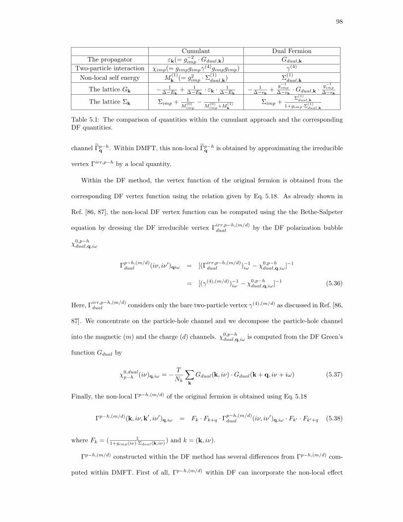
98

Cumulant Dual Fermion

The propagator εk(= g−2imp · Gdual,k) Gdual,k

Two-particle interaction χimp(= gimpgimpγ(4)gimpgimp) γ(4)

Non-local self energy M(1)k (= g2

imp · Σ(1)dual,k) Σ

(1)dual,k

The lattice Gk − 1∆−Ek

+ 1∆−Ek

· εk · 1∆−Ek

− 1∆−ǫk

+g−1

imp

∆−ǫk· Gdual,k · g−1

imp

∆−ǫk

The lattice Σk Σimp + 1

M(0)imp

− 1

M(0)imp+M

(1)k

Σimp +Σ

(1)dual,k

1+gimp·Σ(1)dual,k

Table 5.1: The comparison of quantities within the cumulant approach and the correspondingDF quantities.

channel Γp−hq . Within DMFT, this non-local Γp−h

q is obtained by approximating the irreducible

vertex Γirr,p−h by a local quantity.

Within the DF method, the vertex function of the original fermion is obtained from the

corresponding DF vertex function using the relation given by Eq. 5.18. As already shown in

Ref. [86, 87], the non-local DF vertex function can be computed using the the Bethe-Salpeter

equation by dressing the DF irreducible vertex Γirr,p−h,(m/d)dual by the DF polarization bubble

χ0,p−hdual,q,iω

Γp−h,(m/d)dual (iν, iν′)qiω = [(Γ

irr,p−h,(m/d)dual )−1

iω − χ0,p−hdual,q,iω]−1

= [(γ(4),(m/d))−1iω − χ0,p−h

dual,q,iω]−1 (5.36)

Here, Γirr,p−h,(m/d)dual considers only the bare two-particle vertex γ(4),(m/d) as discussed in Ref. [86,

87]. We concentrate on the particle-hole channel and we decompose the particle-hole channel

into the magnetic (m) and the charge (d) channels. χ0,p−hdual,q,iω is computed from the DF Green’s

function Gdual by

χ0,dualp−h (iν)q,iω = − T

Nk

∑

k

Gdual(k, iν) · Gdual(k + q, iν + iω) (5.37)

Finally, the non-local Γp−h,(m/d) of the original fermion is obtained using Eq. 5.18

Γp−h,(m/d)(k, iν,k′, iν′)q,iω = Fk · Fk+q · Γp−h,(m/d)dual (iν, iν′)q,iω · Fk′ · Fk′+q (5.38)

where Fk = ( 11+gimp(iν)·Σdual(k,iν) ) and k = (k, iν).

Γp−h,(m/d) constructed within the DF method has several differences from Γp−h,(m/d) com-

puted within DMFT. First of all, Γp−h,(m/d) within DF can incorporate the non-local effect

99

beyond DMFT since the DF vertex is constructed from the non-local DF propagator which is

dressed by the non-local DF self energy. Moreover, DF Γp−h,(m/d) depends on three momen-

tum k, k′, and q, i.e., Γp−h,(m/d)(k, iν,k′, iν′)q,iω. Within DMFT, the non-local Γp−h,(m/d) is

computed by assuming Γirr,p−h is local and as a result the non-local vertex depends only on the

momentum transfer q, i.e., Γp−h,(m/d)(iν, iν′)q,iω. Finally, Γp−h,(m/d) calculated from Eq. 5.38

is the full vertex Γfull,p−h in the particle-hole channel, therefore, the irreducible vertex Γirr,p−h

needs to be subtracted to obtained the reducible vertex Γp−h. In principle, Γirr,p−h can be

computed from the full vertex Γfull,p−h by inverting the Bethe-Salpeter equation. We checked

that generally Γirr,p−h is very weakly momentum dependent and one can assume that Γirr,p−h

is local as in DMFT.

The pairing vertex, the irreducible vertex in the particle-particle channel, is constructed

using the non-local Γp−h,(m/d) computed from Eq. 5.38. For the pairing vertex with DF, we

use the full vertex in the particle-hole channel instead of the reducible vertex since Γirr,p−h

is assumed to be local and it does not contribute to the non-local SC gap symmetry such as

s+− or d-wave. Here, we use the same equation relating the pairing vertex with the reducible

vertex function in the particle-hole channel as given in the previous chapter except that the

particle-hole vertex function is computed with the DF method.

The pairing bubble χ0,p−p within the DF method can be computed from the non-local

Green’s function G related to the DF Green’s function Gdual by Eq. 5.13. Since the Green’s

function is dressed by the non-local self energy, χ0,p−p can treat the non-local correlations

beyond DMFT.

χ0,p−p(k, iν) = G↑(k, iν) · G↓(−k,−iν) (5.39)

Within the DF method, both the pairing vertex Γirr,p−p and the pairing bubble χ0,p−p are

computed in a consistent way by treating the non-local correlation effect beyond DMFT. From

the calculated Γirr,p−p and χ0,p−p, one can compute Tc and the SC gap symmetry by solving

the eigenvalue equation of the pairing matrix√

χ0,p−p · Γirr,p−p ·√

χ0,p−p using the Lanczos

algorithm in a same way as used for DMFT.

100

Now, we show that the pairing vertex Γirr,p−p computed using the bare DF Green’s function

G0,dual and the bare DF vertex γ(4) can recover Γirr,p−p obtained within DMFT. Hence, one shot

DF calculation gives DMFT two-particle response functions as defined in the previous chapter.

First, the bare DF polarization bubble in the particle-hole channel χ0,dualp−h (iν)q,iω is the same

as the purely non-local part of the original fermion χ0,p−h i.e., χ0,p−h(iν)q,iω − χ0,p−hloc (iν)iω

χ0,p−hdual (iν)q,iω = − T

Nk

∑

k

G0dual(k, iν) · G0

dual(k + q, iν + iω)

= − T

Nk

∑

k

(g(k, iν) − gloc(iν)) · (g(k + q, iν + iω) − gloc(iν + iω))

= − T

Nk

∑

k

g(k, iω) · g(k + q, iω + iΩ) + T · gloc(iν) · gloc(iν + iω)

= χ0,p−h(iν)q,iω − χ0,p−hloc (iν)iω (5.40)

Also it can be shown that the non-local vertex Γp−h within DF is the same as the non-local

Γp−h computed within DMFT. Since Σdual = 0 at the first shot calculation, the factor Fk =

11+gimp·Σdual

= 1. Therefore, the DF vertex Γp−hdual is the same as the original fermion vertex

Γp−h. The bare DF vertex γ(4) is Γp−hloc (iν, iν′)iω, and Γp−h

dual is obtained by dressing γ(4) by

χ0,dualp−h

Γp−h(iν, iν′)q,iω = Γp−hdual(iν, iν′)q,iω = [(γ(4))−1

iω − (χ0,dualp−h )q,iω]−1

= [(Γp−hloc )−1

iω + (χ0,p−hloc )iω − (χ0,p−h)q,iω]−1

= [(Γirr,p−hloc )−1

iω − (χ0,p−h)q,iω]−1 (5.41)

As a result, the non-local pairing vertex computed within the zeroth order DF method (Σdual =

0) is equal to the pairing vertex within DMFT. Since the pairing bubble χ0,p−p is also same in

both methods, Tc and the gap symmetry results within DMFT are recovered.

101

5.2 The dynamical vertex approximation (DΓA)

5.2.1 Derivation of the approximation

The self energy is the central quantity in the study of correlated many-body systems and it is

related to both a two-particle vertex function Γfull and a Green’s function G by the Schwinger-

Dyson equation [88].

Σ(k, iν) = Unf

2− U

T 2

Nk · Nq

∑

k′,q

∑

iν′,iω

Γfull(k, iν,k′, iν′)q,iω · G(k + q, iν + iω)

·G(k′, iν′) · G(k′ + q, iν′ + iω) (5.42)

Here, nf = T∑

k,iν G(k, iν)eiν·0−

is the occupation number of fermions, Nk is the number of k

points in the Brillouin zone, and T is temperature. The first term of the self energy is calculated

from the lowest order Feynman diagram, so called the Hartree term. This first term accounts

for local and static correlations. The non-local and dynamical correlations are captured by the

second term.

DMFT treats the dynamical correlation on a given site exactly. As a result, the DMFT self

energy is given by the self energy in Eq. 5.42 constructed with the impurity vertex function and

the impurity Green’s function.

Σimp(iν) = Unf

2−UT 2

∑

iν′,iω

Γfullimp(iν, iν′)iω ·Gimp(iν + iω) ·Gimp(iν

′) ·Gimp(iν′ + iω) (5.43)

The main idea of the dynamical vertex approximation (DΓA) [76, 85] is to approximate

the full two-particle vertex function Γfullimp given in Eq. 5.43 by a non-local quantity in order to

incorporate the non-local correlation effect. And also the impurity Green’s function is replaced

by the non-local DMFT Green’s function. Here, we follow the derivation of Ref. [76, 85]. Unlike

the DF method, DΓA does not require additional fermionic degrees of freedom but modify the

self energy diagram directly in order to include the non-local corrections.

The full vertex function Γfullimp contains the diagrams which are reducible in different channels,

i.e., particle-hole channels and particle-particle channels. These vertex functions in different

channels are related to each other by a parquet equation. The fully irreducible vertex function

102

Γf.irrimp can be computed from the full vertex function Γfull

imp by subtracting the reducible vertex

functions in all channels. By assuming that the fully irreducible vertex function is local, the

non-local full vertex function Γfull can be computed by solving the complicated self-consistent

equations of different channels related by the parquet formalism [89].

Instead of solving the full parquet equation, one can concentrate only on the non-local

correlations in particle-hole channels which are strongly enhanced near the antiferromagnetic

region. The full vertex Γfullimp can be represented in terms of the longitudinal (p − h1) channel

and the transverse (p − h2) channel by

Γfullimp = Γf,irr

imp + Γp−h1imp + Γp−h2

imp + Γp−pimp

= Γf,irrimp + (Γfull,p−h1

imp − Γirr,p−h1imp ) + (Γfull,p−h2

imp − Γirr,p−h2imp ) + Γp−p

imp

= Γfull,p−h1imp + Γfull,p−h2

imp − (Γf,irrimp + Γp−h1

imp + Γp−h2imp + Γp−p

imp)

= Γfull,p−h1imp + Γfull,p−h2

imp − Γfullimp (5.44)

Here, Γ represents the reducible diagram (Γ = Γ − Γirr. We also omit spin, momentum, and

frequency indices. In the above derivation, the relations

Γirr,p−h1imp = Γf,irr

imp + Γp−h2imp + Γp−p

imp (5.45)

Γirr,p−h2imp = Γf,irr

imp + Γp−h1imp + Γp−p

imp (5.46)

are used.

The momentum dependence of the full vertex function Γfull,p−himp is obtained by approximat-

ing the local ladder diagram in the particle-hole channel to the non-local one. Namely, the

irreducible vertex Γirr,p−himp is assumed to be local and it is dressed by the non-local polariza-

tion function. This ladder diagram in the particle-hole channel incorporates the non-local spin

fluctuation effect First, the local irreducible vertex Γirr,p−himp is obtained by undressing the local

polarization bubble χ0imp from Γfull,p−h

imp

Γirr,p−h,(m/d)imp (iν, iν′)iω = [(Γ

full,p−h,(m/d)imp )−1

iω + (χ0imp)iω]−1 (5.47)

103

The non-local vertex Γfull,p−hq is obtained by dressing the local Γirr,p−h

imp by the non-local χ0q

Γfull,p−h,(m/d)(iν, iν′)q,iω = [(Γirr,p−h,(m/d)imp )−1

iω − (χ0)q,iω]−1 (5.48)

From the calculated non-local vertex in the particle-hole channel, the local full vertex given in

Eq. 5.44 is approximated to a non-local vertex as

Γfull↑↓↑↓

(iν, iν′)q,iω =1

2(Γfull,p−h1,(m)(iν, iν′)q,iω − Γfull,p−h1,(d)(iν, iν′)q,iω)

+Γfull,p−h2,(m)(iν, iν + iω)k′−k,iν′−iν

−Γfull,(m)imp (iν, iν + iω)iν′−iν (5.49)

Here, we restore the spin, momentum, and frequency indices.

Finally, the non-local self energy Σ(k, iν) is obtained by inserting the non-local vertex func-

tion Γfull↑↓↑↓

q,iωto the local self energy in Eq. 5.43. By changing the indices for the p− h2 channel

such that iν′ → iν + iω, iω → iν′ − iν, the equation for Σ(k, iν) is simplified as

Σ(k, iν) = Unf

2− U

T 2

Nk · Nq

∑

k′,q

∑

iν′,iω

[(3

2Γfull,(m)(iν, iν′)q,iω − 1

2Γfull,(d)(iν, iν′)q,iω)

−Γfull,(m)imp (iν, iν′)iω]G(k + q, iν + iω)G(k′, iν′)G(k′ + q, iν′ + iω) (5.50)

However, one should note that the Green’s function G(k, iν) is still computed within DMFT,

i.e., using the local impurity self energy.

5.2.2 The Moriya λ correction

In the previous subsection, we derived the formula to compute the non-local self energy based

on two-particle vertex functions. However, as shown in Ref. [85], the calculation of the non-local

self energy by Eq. 5.50 overestimates the high frequency result of ImΣ(k, iν) compared to the

exact asymptotic behavior given by.

Σ(iν → ∞) =U2

iν· nf

2· (1 − nf

2) (5.51)

In this subsection, we argue that this asymptotic behavior can be satisfied by imposing a sum

rule in the two-particle level.

104

Here, we impose a sum rule in the two particle level in a similar way as in the two-particle self-

consistent (TPSC) theory [90, 91]. The sum rule requires that the local susceptibility obtained

by summing χ(m/d)q over q and iω is the same as the impurity susceptibility χ

(m/d)imp .

T

Nq

∑

q,iω

χ(m)q,iω = χ

(m)imp(τ = 0+) = 〈(n↑

f − n↓f )2〉 = nf − 2〈n↑

f · n↓f 〉 (5.52)

T

Nq

∑

q,iω

χ(d)q,iω = χ

(d)imp(τ = 0+) = 〈(n↑

f + n↓f )2〉 − 〈(n↑

f + n↓f )〉2 = nf + 2〈n↑

f · n↓f 〉 − n2

f (5.53)

Here, the Pauli principle is used for the rightmost result, i.e., 〈(nσf )2〉 = 〈nσ

f 〉.

The non-local susceptibility χ(m/d)q is computed by dressing the non-local polarization func-

tion χ0q the local irreducible vertex Γirr

loc . The local susceptibility obtained by averaging χ(m/d)q

over q vectors is not the same as the impurity susceptibility χ(m/d)imp since

1

Nq·∑

q

χ(m/d)(q, iω) =T 2

Nq·∑

q

∑

iν,iν′

1

(χ0)−1q,iω − Γ

irr,(m/d)imp

6= T 2

Nq·

∑

iν,iν′

1∑

q(χ0)−1q,iω − Γ

irr,(m/d)imp

= χ(m/d)imp (iω). (5.54)

Therefore, the sum rules in Eq. 5.52 and 5.53 are not satisfied. The averaged susceptibility over

q is the same as the impurity one only in the infinite dimension where the lattice problem is

mapped to the impurity problem.

In order to satisfy the sum rules in Eq. 5.52 and 5.53, we introduce the Moriya λ correction

in order to incorporate the spin fluctuation effect. This Moriya λ term within DΓA is employed

in Ref. [85]. In the self-consistent renormalization theory of spin fluctuation[cite], this λ term

takes into account the feedback of the spin fluctuation and in principle it can be computed from

the magnetic susceptibility of the system. For simplicity, we determine this λ term to satisfy

the sum rules in Eq. 5.52 and 5.53. This Moriya λ correction is given only for the magnetic

channel and at the zero iω frequency where the spin fluctuation is dominant. Also we assume

λ is local i.e., λ(m)q ≈ λ(m).

T 2

Nq

∑

q

∑

iν,iν′

1

(χ0)−1q,iω − Γ

irr,(m)imp + λ

= χ(m)imp(iω) (5.55)

105

Now we show that the Moriya λ correction satisfying the sum rule in Eq. 5.55 also produces

the exact high frequency asymptotic of the self energy. The non-local self energy in Eq.5.51 can

be calculated using the particle-hole ladder diagram renormalized by Moriya λ term. If only

one frequency of the irreducible vertex Γirrp−h approaches ∞ while other frequencies are finite,

Γirrp−h can be replaced by the bare interaction, i.e,

Γirr,(m/d)p−h (iν → ∞, iν′)iω ≈ (∓)U. (5.56)

The bare interaction is −U for the magnetic channel and +U for the charge channel. Using

Eq. 5.56, the self-energy in Eq. 5.50 in the limit of iν → ∞ can be simplified as

Σ(k, iν → ∞) = Unf

2+

U2

2

T

Nq

∑

q,iω

((3

2χ

(m)q,iω +

1

2χ

(d)q,iω) − χ

(m)imp,iω

)· G(k + q, iν + iω) (5.57)

since Γirrp−h connected with G(k + q, iν + iω) can be replaced by the bare interaction.

Using the sum rules in Eq. 5.52 and 5.53, one can show that the high frequency asymptotic

behavior of the DΓA self energy is given by the exact formula in Eq. 5.51.

Σ(k, iν → ∞) = Unf

2+

U2

2 · iνT

Nq

∑

q,iω

((3

2χ

(m)q,iω +

1

2χ

(d)q,iω) − χ

(m)imp,iω

)

= Unf

2− U2

4 · iν T∑

iω

(χ(m)imp,iω + χ

(d)imp,iω)

= Unf

2− U2

iν

nf

2(1 − nf

2) (5.58)

5.2.3 The calculation scheme

Unlike the DF method, DΓA is a non-conserving approximation. The DΓA self energy is com-

puted using DMFT G(k, iν) instead of taking the feedback from the DΓA non-local Green’s

function. Therefore, the DΓA calculation is performed in a non-self-consistent way. The fully

self-consistent calculation requires the solution of the complicated full parquet equation. Nev-

ertheless, the sum rule in the two-particle level is enforced by the Moriya λ term. Since this

Moriya λ term already includes the non-local fluctuation effect beyond DMFT, the non-self-

consistent solution of DΓA will be more reliable. The calculation procedure of DΓA is given as

follows.

106

CTQMC

Compute Gimp, impkGDMFTk =Gimp ?

CTQMC

Compute imp, Gimp

Compute Moriya ,non-local ph,q,i

Compute (k,i), G(k,i)T

Nk

k,iG(k,i)ei·0=n ?

Compute new

Compute new

no

no

yes

Figure 5.2: The calculation procedure of DΓA.

107

1. First, the DMFT self-consistent loop is continued until the convergence is reached.

∑

k

1

iν + µ − ǫk − Σ=

1

iν + µ − ∆ − Σ(5.59)

2. Once the DMFT solution is converged, CTQMC samples the impurity two-particle vertex

function Γp−h from the converged hybridization ∆ and the chemical potential µ. The

impurity irreducible vertex function Γirrp−h is computed from the full vertex Γp−h using

Eq. 5.47.

3. The non-local vertex function in the magnetic/charge channel Γfull,(m/d)p−h,q,iω is computed by

dressing Γirrp−h with the non-local polarization function (χ0)q,iω (Eq. 5.48).

4. In order to satisfy the sum rule in the two-particle level, the Moriya λ correction is

determined from the Eq. 5.55.

5. Finally, the non-local self energy Σ(k, iν) within DΓA is computed using Eq. 5.50. And

from Σ(k, iν), the non-local Green’s function G(k, iν) can be computed. In the fixed

density n calculation, the chemical potential µ is adjusted to satisfy that the density

computed within DΓA is the same as the desired n.

T

Nk

∑

k,iν

G(k, iν)eiν0−

= n (5.60)

Using this new µ, the DMFT loop starts again by going back to the step 1.

5.2.4 The pairing susceptibility within DΓA

Within DΓA, the non-local fluctuation beyond DMFT is taken into account by computing the

non-local self energy using Eq.5.50. And the one-particle Green’s function is dressed by this DΓA

self energy. In the two-particle level, the non-local fluctuation is treated by the Moriya λ term

in order to satisfy the sum rule in Eq. 5.55. Unlike the DF method, the non-local fluctuations

included in the self-energy and the vertex function are not treated in a self-consistent way.

For computing the pairing susceptibility within DΓA, both the pairing vertex and the pairing

bubble includes the non-local correlations beyond DMFT. The pairing vertex Γirr,p−p(k, iν,k′, iν′)

108

computed within DΓA is computed with the same equation as the DMFT pairing vertex is

computed except that the Moriya λ correction is included to satisfy the sum rule in Eq. 5.55.

Therefore, the reducible vertex in the particle-hole channel Γ is given by

Γp−h,(m/d)(iν, iν′)q,iω =∑

iν1,iν2

Γirr,p−h,(m/d)(iν, iν1)iω·χp−h,(m/d)(iν1, iν2)q,iω·Γirr,p−h,(m/d)(iν2, iν′)iω

(5.61)

where χ is the renormalized susceptibility due to the Moriya λ term.

χp−h,(m)(iν1, iν2)q,iω = [(χ0,p−h)−1q,iω − Γirr,p−h,(m) + λ]−1(iν1, iν2)q,iω (5.62)

As a result, the pairing vertex within DΓA is renormalized from the DMFT pairing vertex by

the λ correction.

The DΓA pairing bubble χ0,p−p(k, iν) is computed using the non-local DΓA Green’s function

which is dressed by the DΓA self energy obtained by Eq. 5.50.

χ0,p−p(k, iν) = G↑(k, iν) · G↓(−k,−iν) (5.63)

G(k, iν) =1

iν + µ − ǫk − Σ(k, iν)(5.64)

Finally, the pairing susceptibility is computed by dressing the pairing bubble χ0,p−p(k, iν)

by the pairing vertex Γirr,p−p(k, iν,k’, iν′). Tc and the SC gap symmetry can be computed by

solving the eigen-problem of the pairing matrix√

χ0,p−p · Γirr,p−p ·√

χ0,p−p using the Lanczos

algorithm.

109

Chapter 6

The Application of the Two-particle Vertex Calculation :

Model Hamiltonians

In this chapter, we compute the phase diagram of magnetism and superconductivity in the

Hubbard model and the periodic Anderson model. For the calculation of the superconducting

(SC) critical temperature Tc and the SC gap symmetry, we apply the two-particle vertex func-

tion approach derived in Chapter 4 and Chapter 5 to the model Hamiltonian calculation. Tc is

computed as a function of the doping for the Hubbard model and as a function of the hybridiza-

tion for the periodic Anderson model. The pairing vertex and the pairing bubble are computed

within the DMFT method, and for comparison, DΓA and DF methods are also employed to

incorporate the non-local correlations beyond DMFT. We show that the SC phase is stable near

the region where the magnetic fluctuation is strong and that the non-local methods reduce Tc

compared to a DMFT result due to the renormalized pairing interaction. To further analyze

Tc and the SC gap symmetry results, we also compute the momentum dependent magnetic

susceptibility, the Fermi surface, the effective U , and other relevant quantities.

6.1 The Hubbard Model

6.1.1 The Hamiltonian

The Hubbard model describes the strongly correlated physics in cuprates where doping an

electron or a hole induces high Tc superconductivity. This model consists of the kinetic energy

term due to the hopping of fermions to adjacent sites and the on-site Coulomb energy term.

110

We consider the 2D one-band Hubbard model whose Hamiltonian is given as follows.

H =∑

k,σ

(ǫ(k) − µ) · f†k,σfk,σ + U ·

∑

i

f†i,↑f

†i,↓fi,↓fi,↑ (6.1)

ǫ(k) = −2t(cos(kx) + cos(ky)) − 4t′ cos(kx) cos(ky) (6.2)

The on-site Coulomb interaction U is set to 12t where t is the nearest-neighbor hopping inter-

action. And the next-nearest hopping t′ is fixed as -0.3t. These parameters exhibit the Mott

insulating state accompanying with the antiferromagnetic state at the half-filling (n = 1). As

the system is doped away from the half-filling, it is known that the magnetic state is suppressed

and the superconducting state emerges. In this section, we compute the critical temperature Tc

and the gap symmetry of superconductivity in the hole doping (δ = 1 − n) region of the Hub-

bard model by applying the vertex function approach based on DMFT and non-local methods

beyond DMFT.

6.1.2 The phase diagram of antiferromagnetism and superconductiv-

ity

Fig.6.1 displays the phase diagram of antiferromagnetism (AFM) and d-wave superconductivity

(SC) in the hole-doped region of the Hubbard model. The Neel temperature (TN ) of the AFM

state is determined as the temperature where DMFT magnetic susceptibility at the ordering

(π, π) vector diverges. Tc of SC is calculated using different methods. Within the DMFT

method, the pairing vertex Γirr,p−p(k, iν,k′, iν′) is computed by dressing the DMFT irreducible

particle-hole vertex Γirr,p−h with the non-local polarization bubble χ0,p−hq . χ0,p−h

q is computed

from DMFT G(k, iν) dressed by a local self-energy. The pairing bubble χ0,p−p in the particle-

particle channel is computed from the same G(k, iν). The DMFT+λ method renormalizes the

pairing vertex by a Moriya λ term to satisfy the sum rule in the two-particle level. However,

DMFT χ0,p−p is still used. The DΓA method uses this renormlized pairing vertex and χ0,p−p

computed from G(k, iω) dressed by a non-local DΓA self energy. Within the DF method, the

pairing vertex and the pairing bubble diagram are derived from the DF vertex and the DF

111

0.00 0.05 0.10 0.15 0.200.00

0.05

0.10

0.15

0.20

0.25

0.30

0.35

T/t

AFM

Tc DMFT

Tc DMFT+ Tc D!ATc DF

TN DMFT

Tincom

Figure 6.1: The phase diagram of the antiferromagnetic Neel temperature (TN ) and the super-conducting critical temperature (Tc) in the one-band Hubbard model. The x-axis is the holedoping (δ) and the y-axis is the temperature T . TN (black square) is determined within DMFT.As δ increases, TN is suppressed and the commensurate (π, π) magnetic peak changes to the

incommensurate peak (dashed line). Tc is calculated using DMFT (black triangle), DMFT+λ(blue diamond), DΓA (red square), and DF (green circle) methods. d-wave superconductivityemerges near the magnetic phase.

112

bubble by an exact relation. Both DF quantities are determined in a self-consistent way as a

conserving approximation.

Fig. 6.1 shows that TN computed within DMFT (black square) is decreasing as the doping

(δ) increases, and above δ=0.14 TN is completely suppressed down to T=0. This decrease of

the magnetic susceptibility at the large doping is mainly due to the screened Γirr,p−h. Namely,

Γirr,p−h is screened by the ladder diagram in the particle-particle channel[92] and this screening

becomes more enhanced at larger dopings where the quasi-particles are coherent. The magnetic

ordering vector is (π, π) due to the nesting of the Fermi surface. This ordering vector changes

from the commensurate (π, π) vector to the incommensurate (π− ε, π− ε) and (π, π− ε) vector

near δ=0.15. This incommensurate magnetism is caused by the frustration due to the doping

and, as a result, the change of Fermi surface nesting vector (see Fig. 6.6).

Tc of the SC state is computed using various methods as the temperature at which the

eigenvalue of the pairing matrix reaches one. The result shows that the d-wave SC state is

stabilized near the magnetic phase where the strong magnetic fluctuation causes the pairing

interaction of Cooper pairs. Within the DMFT method, Tc (black triangle in Fig. 6.1) shows a

strong enhancement even in the underdoped region (δ=0.05). Tc decreases as δ increases and it

becomes completely 0 above δ=0.18. The experimental phase diagram of Tc shows the strong

suppression of Tc in the underdoped region and as a result the dome shape with the maximum

of Tc at the optimal doping.

Within DMFT, the overestimated Tc in the underdoped region can be caused by mainly

two reasons. First, the pairing interaction is overestimated within DMFT. TN computed within

DMFT is exaggerated since the non-local fluctuation effect is neglected. This enhanced TN

causes the strong pairing interaction even in the underdoped region. Second, the pseudo gap

physics is not captured within DMFT. In the underdoped region, ARPES experiments found the

reduction of spectral weight at the Fermi energy, namely the pseudo-gap. The opening of this

pseudo gap will decrease Tc due to the suppression of the pairing bubble, χ0,p−p. Nevertheless,

in the overdoped region (δ¿0.125) where this pseudo gap physics becomes less important, the

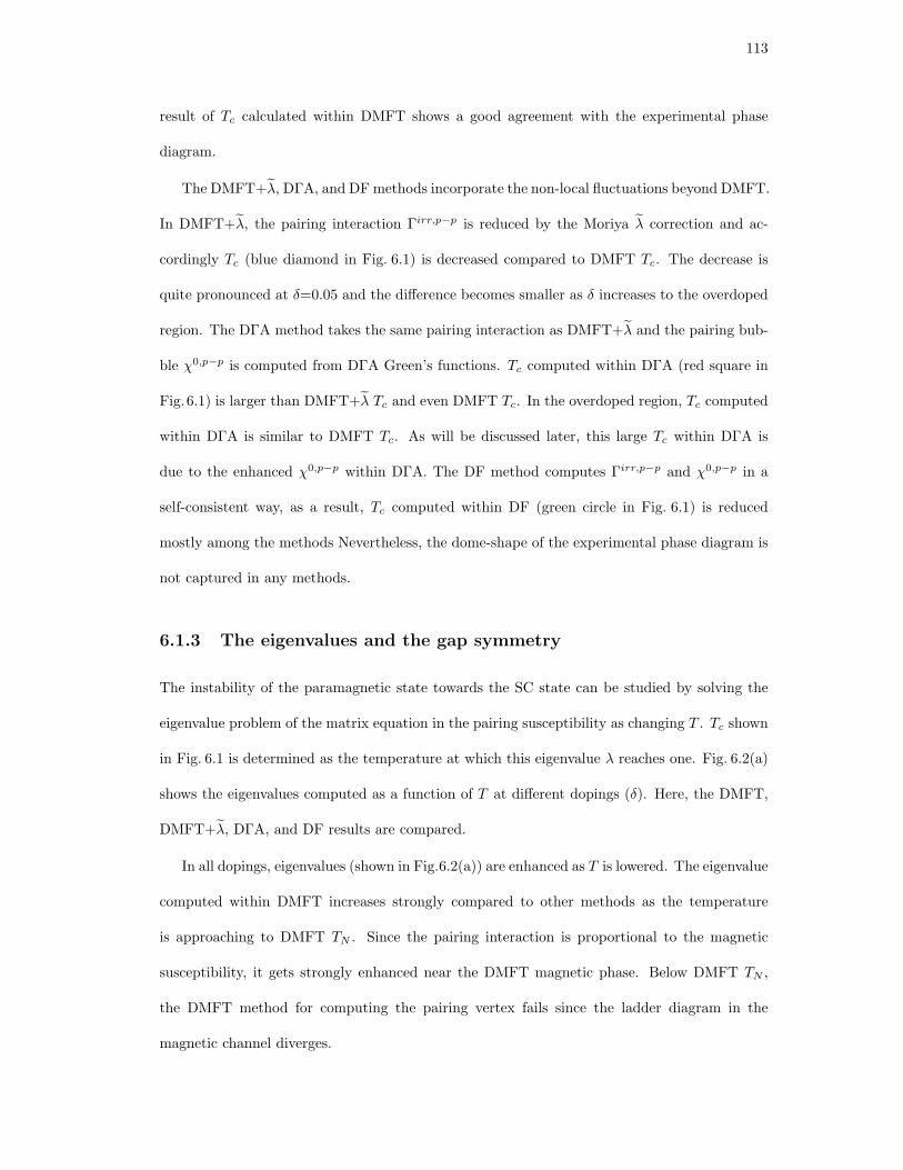
113

result of Tc calculated within DMFT shows a good agreement with the experimental phase

diagram.

The DMFT+λ, DΓA, and DF methods incorporate the non-local fluctuations beyond DMFT.

In DMFT+λ, the pairing interaction Γirr,p−p is reduced by the Moriya λ correction and ac-

cordingly Tc (blue diamond in Fig. 6.1) is decreased compared to DMFT Tc. The decrease is

quite pronounced at δ=0.05 and the difference becomes smaller as δ increases to the overdoped

region. The DΓA method takes the same pairing interaction as DMFT+λ and the pairing bub-

ble χ0,p−p is computed from DΓA Green’s functions. Tc computed within DΓA (red square in

Fig.6.1) is larger than DMFT+λ Tc and even DMFT Tc. In the overdoped region, Tc computed

within DΓA is similar to DMFT Tc. As will be discussed later, this large Tc within DΓA is

due to the enhanced χ0,p−p within DΓA. The DF method computes Γirr,p−p and χ0,p−p in a

self-consistent way, as a result, Tc computed within DF (green circle in Fig. 6.1) is reduced

mostly among the methods Nevertheless, the dome-shape of the experimental phase diagram is

not captured in any methods.

6.1.3 The eigenvalues and the gap symmetry

The instability of the paramagnetic state towards the SC state can be studied by solving the

eigenvalue problem of the matrix equation in the pairing susceptibility as changing T . Tc shown

in Fig. 6.1 is determined as the temperature at which this eigenvalue λ reaches one. Fig. 6.2(a)

shows the eigenvalues computed as a function of T at different dopings (δ). Here, the DMFT,

DMFT+λ, DΓA, and DF results are compared.

In all dopings, eigenvalues (shown in Fig.6.2(a)) are enhanced as T is lowered. The eigenvalue

computed within DMFT increases strongly compared to other methods as the temperature

is approaching to DMFT TN . Since the pairing interaction is proportional to the magnetic

susceptibility, it gets strongly enhanced near the DMFT magnetic phase. Below DMFT TN ,

the DMFT method for computing the pairing vertex fails since the ladder diagram in the

magnetic channel diverges.

114

0.0

0.5

1.0

1.5

2.0"(a) #=0.05DMFTDMFT+$D%ADF

#=0.1

0.15 0.20 0.25 0.30T/t

0.0

0.5

1.0

1.5" #=0.0750.05 0.10 0.15 0.20 0.25

T/t

#=0.125

&'0 '&'0

'(b)-

+

-

+((k)()=0.125,T/t=0.1)

*0.08*0.040.00

0.04

0.08

Figure 6.2: (a) The eigenvalue λ of the pairing susceptibility in the particle-particle channelas a function of T at different dopings (δ=0.05, 0.075, 0.1, and 0.125). DMFT, DMFT+λ,DΓA, and DF methods are employed for computing the eigenvalues. (b) The eigenfunctionφ(k) computed at δ=0.125 and T=0.1t. This φ(k) of the leading eigenvalue corresponds to theSC gap function.

115

The DMFT+λ, DΓA, and DF methods show a rather slow increase of eigenvalues compared

to DMFT due to the non-local correlation effect. The eigenvalue computed within DΓA is

the largest among at T above Tc in all dopings. As T gets lowered, DMFT eigenvalue is

enhanced sharply. The eigenvalue computed within the DMFT+λ method is similar as the

DMFT eigenvalues at T > Tc and they are strongly reduced as T is lowered since the Moriya

λ correction gets larger. The DF eigenvalues are the smallest in all dopings since the pairing

interaction is strongly reduced due to the non-local correlation treated by dual fermions.

As the doping increases, the eigenvalues computed from all methods are reduced showing

an agreement with the monotonic decrease of Tc in Fig. 6.1. This monotonic behavior mainly

originates from the suppression of the pairing interaction at increased doping. As we will show

below, the pairing interaction is quite sensitive to the change of dopings.

The momentum dependence of the eigenfunction φk corresponding to the leading eigenvalue

shows the gap symmetry of the SC state. Fig. 6.2(b) shows the eigenfunction φ(k, iν = πT )

in the Brillouin zone. Within DMFT, the momentum dependence of φ clearly shows that the

gap symmetry is d-wave, i.e., cos kx − cos ky. Indeed, the gap symmetry of superconductivity

in the one-band Hubbard model has been studied by many theoretical works to be a d-wave.

We found that the leading eigenfunction has always d-wave symmetry in all doping parameters

shown in Fig. 6.1 and in all methods. Therefore, we confirmed the d-wave symmetry of the SC

gap is mostly favored in the one-band Hubbard model compared to other symmetries.

6.1.4 The pairing strength and the pairing bubble

Fig. 6.3 shows the temperature dependence of the projected pairing interaction Γp−p,(d) at dif-

ferent dopings. The d wave projection of the pairing interaction is the largest among symmetry

channels at all dopings, therefore, only Γp−p,(d) results are shown.

In the DMFT method, Γirr,p−p is obtained from the reducible diagram in the particle-hole

channels, i.e., Γirr,p−h · χp−h · Γirr,p−h. As a result, Γp−p,(d) gets dominant near DMFT TN

where the magnetic χp−h is strongly enhanced.

116

0

40

80

120

¯

+p,p,(d) -=0.05 -=0.1

0.15 0.20 0.25 0.30T/t

0

40

80

¯

+p,p,(d) -=0.0750.05 0.10 0.15 0.20 0.25

T/t

-=0.125DMFTD.ADF

Figure 6.3: The pairing interaction projected to the d wave channel, Γp−p,(d) as a function oftemperature at different dopings. The results employing the DMFT, DΓA, and DF methodsare compared.

In the DΓA method, χp−h is renomalized from the DMFT value by the Moriya λ correction

to satisfy the sum rule in the two-particle level. In principle, this λ correction renormlizes

TN down to zero satisfying the Mermin-Wagner theorem in a 2D system [85]. At δ=0.05,

Γp−p,(d) is renormlized from quite high T and becomes strongly renormalized at lower T . As

the doping increases, this λ correction becomes effective only at lower temperatures where

magnetic fluctuation is strong.

The DF method take into account the non-local correction of the vertex function self-

consistently in a conserving way. As a result, Γp−p,(d) is strongly renormlized in the DF method

at all dopings compared to either the DMFT or the DΓA method. In the DΓA calculation, the

fully self-consistent calculation without the Moriya λ term should renormalize Γp−p,(d) further

as the DF method.

As doping increases, Γp−p,(d) decreases monotonically in all methods, i.e., the pairing in-

teraction is the strongest at the underdoped region (δ=0.05). This result is related to the

overestimated Tc in the underdoped region. This monotonic increase of Γp−p,(d) is also shown

in the DCA calculation[93]. Nevertheless, the DCA calculation can produce the dome shape

117

of Tc due to the strong reduction of χ0,p−p in the underdoped region. It is also possible that

Γp−p,(d) results computed within the DMFT, DΓA, and DF methods are still overestimated in

the underdoped region even at high temperatures compared to the DCA method.

0.05

0.10

0.15

0.20/0,p0p 1=0.05DMFTD2ADF

1=0.1

0.0 0.1 0.2T/t

0.05

0.10

0.15/0,p0p 1=0.0750.0 0.1 0.2 0.3

T/t

1=0.125Figure 6.4: The pairing bubble in the particle-particle channel χ0,p−p projected to the d-wavesymmetry channel. The result is obtained as a function of T at different dopings. The DMFT,DΓA, and DF methods are used for the calculation.

Fig. 6.4 displays the temperature dependence of χ0,p−p at δ=0.05, 0.75, 0.1, and 0.125. The

DMFT, DΓA, and DF methods are employed for calculation. At all dopings, χ0,p−p computed

within the non-local methods shows the larger value compared to the DMFT method. This

result somehow contradicts with the half-filling Hubbard model results where DΓA and DF

methods produce a spin gap at the Fermi energy [85, 94] and as a result the reduction of χ0,p−p.

The eigenvalue in the pairing channel is determined by the combination of Γp−p,(d) and

χ0,p−p. Even though the DF method gives the largest χ0,p−p compared to other method, the

strong suppression of Γp−p,(d) results in the lowest eigenvalue and, as a result, the lowest Tc at

all dopings. In the DΓA method, χ0,p−p is quite enhanced than DMFT, but slightly smaller

than DF χ0,p−p. However, Γp−p,(d) within DΓA is not strongly suppressed as DF, therefore, Tc

within DΓA is even nslightly higher than DMFT Tc. It is suggested that χ0,p−p within cluster

DMFT can be strongly enhanced at the optimal doping within cluster DMFT [93].

118

In the DMFT result, the temperature dependence of χ0,p−p near the optimal doping (δ ∼0.125)

reveals the logarithmic enhancement at low temperatures showing an agreement with the Fermi

liquid behavior of χ0,p−p ∼ log(1/T ). In the BCS argument, this logarithmic enhancement of

χ0,p−p at low temperature gives the pairing instability for a given interaction whose energy

scale is limited by the phonon Debye frequency. At the underdoped region (δ=0.05,0.075), this

logarithmic enhancement is not clearly present even at low T . This is due to the fact that

quasi-paritcles computed within DMFT in the doped Mott insulating region show an incoher-

ent behavior until the very low T is reached. In spite of the incoherent χ0,p−p, the pairing

interaction Γp−p,(d) within DMFT is strong enough to cause the pairing instability at high T

in our calculation.

In the cluster DMFT calculation with large cluster sites, χ0,p−p in the underdoped region

is strongly suppressed compared to the optimal region due to the pseudo-gap in the density

of states [93]. In the DΓA and DF methods, the pseudo-gap is not clearly seen even at the

underdoped region (δ=0.05) (see Fig. 6.6(b)) until the lowest temperature we could reach.

Therefore, stronger fluctuation is expected to be included in DΓA and DF methods. The current

DΓA method needs to be implemented as a fully self consistent way without the need of Moriya

λ correction. In DF method, the strong non-local fluctuation can be included by computing

more relevant diagrams for the DF self energy. For example, the ladder type diagram in the

particle-hole channel is possible. The study of superconductivity in the underdoped region by

including the strong non-local fluctuation will be the future challenge.

6.1.5 The magnetic susceptibility and the spectral function

Fig. 6.5 shows χm(q) along the special q path chosen in the Brillouin zone at δ=0.05 and 0.15.

At δ=0.05, χm(q) shows a peak at (π, π) in all methods while this peak is splitted to (π−ε, π−ε)

and (π, π − ε) at δ=0.15. The left figure in Fig. 6.6(a) displays the spectral function at δ=0.05.

Although the spectral weight is rather small and broad compared to δ=0.15, this Fermi surface

reveals that the particle-hole excitation is dominant at q=(π, π). Within DΓA and DF, χm(q)

119

0

10

20

30

403m (q) 4=0.05

T=0.2t

(a) DMFTD5ADF

(0,0) (6,6) (6,0) (0,0)q

0

2

4

6

83m (q) 4=0.15

T=0.05t

(b)

Figure 6.5: The magnetic susceptibility χmq computed in the Hubbard model as a function

of the momentum transfer q at different dopings. The susceptibilities are computed withinDMFT, DΓA, and DF methods for a comparison. (a) The doping δ=0.05 and T=0.2t. (π, π)antiferromagnetism is strongly enhanced. (b) δ=0.15 and T=0.05t. The susceptibility at (π, π)is suppressed and the magnetic ordering vector is splitted to (π − ε, π − ε) and (π, π − ε).

780 87808(a) 9=0.05,DMFT

0.0

0.5

1.0

1.5

780 87808

(:;<,:;<)9=0.15,DMFT

0

1

2

780 87808(b) 9=0.05,DF

0.0

0.4

0.8

780 878089=0.05,D=A

0.0

0.4

0.8

Figure 6.6: The spectral function A(k, ω = 0) = − 1π G(k, ω = 0) in the Hubbard model. (a)

A(k) computed within DMFT at δ=0.05 (left) and 0.15 (right). T=0.02t in both dopings. (b)A(k) computed with the non-local methods beyond DMFT at δ=0.05 and T=0.1t. The DF(left) and the DΓA (right) methods are used.

120

especially at q=(π, π) is strongly decreased due to the non-local effect and as a result, the

pairing interaction is also suppressed as shown in Fig. 6.3. Even though χm(q) is slightly more

reduced within DΓA, the pairing interaction is more suppressed in the DF method.

This q dependence of the magnetic susceptibility χm(q) is related to the momentum de-

pendence of the pairing vertex. The (π, π) peak of χm(q) indicates that the pairing interaction

is strongly enhanced between Cooper pairs at k and k′ with k − k′ = (π, π). We checked

that the contribution to the pairing vertex from the charge channel is much smaller than the

magnetic channel. This momentum dependence of the pairing vertex plays a crucial role to

determine the SC gap symmetry. Namely, quasi-particles near the Fermi surface at k = (±π, 0)

and k′ = (0,±π) (see the Fermi surface in Fig. 6.6(a)) are strongly affected by the pairing

interaction induced from (π, π) magnetism. As a result, the gap function is maximum at those

anti-nodal (±π, 0) and (0,±π) points and the gap changes even a sign going from the k point

to the k′ point for the pairing interaction to be effectively attractive. Therefore, the d-wave

symmetry, cos(kx) − cos(ky), is favored in the Hubbard model.

As δ increases to 0.15, the position of the magnetic peak changes from (π, π) to (π−ε, π−ε)

and (π, π − ε) . This incommensurate magnetism originates from the nesting vector of the

Fermi surface at this doping. Fig. 6.6(a) shows that the Fermi surface is slightly shrinked as

δ increases and as a result the nesting vector is pronounced at (π − ε, π − ε) shown as the

white arrows. Within DΓA and DF, χm(q) is reduced due to the non-local fluctuation and the

pairing interaction as well (Fig. 6.3). Nevertheless, this incommensurate magnetism still favors

the d-wave SC symmetry as shown in the phase diagram.

Fig. 6.6(b) shows the spectral function at δ=0.05 computed within the non-local methods,

DF and DΓA. T is set to 0.1t which is higher than T at Fig. 6.6(a). Due to this high T , the

spectral weight is heavily reduced and quite broad. Nevertheless, the formation of the Fermi arc

due to the non-local effect is still noticeable. Namely, the spectral weight at (±π2 ,±π

2 ) is slightly

enhanced than the (±π, 0) and (0,±π) points. This Fermi arc formation does not necessarily

reduce the paring bubble χ0,p−p compared to DMFT χ0,p−p since the overall spectral weight

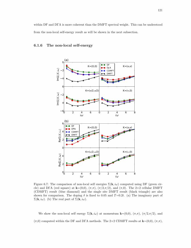
121

within DF and DΓA is more coherent than the DMFT spectral weight. This can be understood

from the non-local self-energy result as will be shown in the next subsection.

6.1.6 The non-local self-energy

>6>4>20

Im

?(K,i@) (a)

K=(0,0) K=(A,A)DFDBACDMFTDMFT

0 2 4 6iC>6>4

>2Im

?(K,i@) K=(A/2,A/2)0 2 4 6 8

iCK=(A,0)

0

2

4

6

Re

D(K,iE) (b)

K=(0,0)DFDFACDMFTDMFT

K=(G,G)

0 2 4 6iH0

2

4

Re

D(K,iE) K=(G/2,G/2)0 2 4 6 8

iHK=(G,0)

Figure 6.7: The comparison of non-local self energies Σ(k, iω) computed using DF (green cir-cle) and DΓA (red square) at k=(0,0), (π,π), (π/2,π/2), and (π,0). The 2×2 cellular DMFT(CDMFT) result (blue diamond) and the single site DMFT result (black triangle) are alsoshown for comparison. The doping δ is fixed to 0.05 and T=0.2t. (a) The imaginary part ofΣ(k, iω). (b) The real part of Σ(k, iω).

We show the non-local self energy Σ(k, iω) at momentum k=(0,0), (π,π), (π/2,π/2), and

(π,0) computed within the DF and DΓA methods. The 2×2 CDMFT results at k=(0,0), (π,π),

122

and (π,0) are also shown for the consistency check. Fig. 6.7 (a) displays the imaginary part

of Σ(k, iω). In both the DF and DΓA methods, the scattering rate ImΣ(ω = 0) at (0,0) gets

smaller compared to other momentums namely more coherent while (π,π) self energies are quite

incoherent due to the non-local correlations. Both methods give a good agreement with the

CDMFT result.

Comparing k=(π/2,π/2) and k=(π,0), ImΣ at (π,0) has slightly larger scattering rate than

k=(π/2,π/2). This momentum differentiation cause the Fermi arc shape shown in Fig. 6.6(b).

At both (π/2,π/2) and (π,0), DΓA results shows a slightly more incoherent Σ(k, iω) than DF

results. Nevertheless, both ImΣ data show the smaller scattering rate than the DMFT ImΣ.

Our result shows that quasi-particles get more coherent at high temperatures in the underdoped

region due to the non-local effect. This also coincides with the enhanced χ0,p−p within DF and

DΓA methods compared to DMFT shown in Fig. 6.3.

Fig. 6.7(b) shows the real part of Σ(k, iω). At k=(0,0), the DF result shows a better

agreement with the CDMFT result while the DΓA ReΣ is below the DF ReΣ. Since ǫk +ReΣk

shows the effective quasi-particle energy, (0,0) orbital computed within DΓA is located more

away from the Fermi energy compared to DF and CDMFT. The (π,π) orbital within DF also

agrees well with the CDMFT result while the (π,π) orbital within DΓA is slightly increased. At

both (π/2,π/2) and (π,0), ReΣ within DF and DΓA show a good agreement with DMFT and

CDMFT results even though DF result is slightly enhanced at low energy.

6.1.7 The effective U

In Fig. 6.8, Ueff in the magnetic channel is shown as a function of T at different dopings (δ).

The formula for Ueff is given in subsection 4.5.3. As the doping δ increase, Ueff is more

renormalized due to the dynamical screening from coherent quasi-particles at large dopings. In

the underdoped region (δ=0.05), Ueff is even greater than the bare interaction 12t shown as

the dashed line in Fig. 6.8. This strong Ueff at δ=0.05 causes the strong pairing interaction

even at high T (Fig. 6.3) and hence the high Tc in the underdoped region. In real materials,

123

0.0 0.1 0.2 0.3 0.4T/t

6

8

10

12

14

16

18

Ueff/t

I=0.05I=0.075I=0.1I=0.125

Figure 6.8: The effective interaction (Ueff ) for the electron-magnon coupling calculated as afunction of T at different dopings (δ=0.05, 0.75, 0.1, and 0.125) in the Hubbard model. Thedashed line marks the bare interaction U .

the strong interaction among d or f electrons can be renormlized due to screening channels

with other conduction electrons, therefore this strongly enhanced Ueff might be the artifact of

the single orbital model calculation. As T is lowered, the renormalization of Ueff gets more

stronger since the coherence scale is also increased.

Our result of Ueff shows a similar feature compared to the cluster DMFT and the QMC

results[95, 96]. Namely, Ueff decreases as δ gets larger and T is cooled down. The cluster DMFT

result shows even more renormalized Ueff in the underdoped region This can be caused by the

strong non-local correlation treated within cluster DMFT. The cluster DMFT result also shows

a slight upturn of Ueff at very low T which might be due to the pseudo-gap physics which

DMFT cannot capture. Nevertheless, Ueff computed within DMFT reveals a qualitatively

similar feature as the Ueff within cluster DMFT, hence the pairing interaction as well.

124

6.2 The Periodic Anderson Model

6.2.1 The Hamiltonian

The periodic Anderson model treats strongly correlated fermions (f) with the on-site Coulomb

interaction U , which are hybridized with non-interacting fermions (c) by the hybridization

function V (k). This model is adequate for describing materials such as the heavy fermion

system containing open shells of d or f electrons and the broad s, p or d bands near the Fermi

energy. Here, we consider the 2D two-band (one f and one c) periodic Anderson model. The

Hamiltonian for the periodic Anderson model is given by

H =∑

k,σ

(ǫf (k) − µ) · f†k,σfk,σ + U ·

∑

i

f†i,↑f

†i,↓fi,↓fi,↑

+∑

k,σ

(ǫc(k) − µ) · c†k,σck,σ +∑

k,σ

V (k) · (f†k,σck,σ + c†k,σfk,σ) (6.3)

where

ǫf (k) = ǫ0f + 2ǫf (cos(kx) + cos(ky)) + 4ǫ′f cos(kx) cos(ky) (6.4)

ǫc(k) = 2ǫc(cos(kx) + cos(ky)) + 4ǫ′c cos(kx) cos(ky) (6.5)

V (k) = Vk(1 − cos(kx) cos(ky)) (6.6)

The on-site energy ǫ0f is -7.8ǫc where ǫc is the nearest-neighbor hopping energy of c electrons, the

hopping energy of f electrons ǫf=0.15ǫc, the next-nearest neighbor hopping energy ǫ′f=0.3ǫf ,

the next-nearest hopping energy of c electrons ǫ′c=0.3ǫc, the on-site Coulomb interaction U=8ǫc,

and the chemical potential µ=-0.4ǫc. Note that f electrons also have the hopping energy

term unlike the typical periodic Anderson model. The hybridization parameter Vk controls

correlations of f electrons from the strong correlation limit at small Vk to the weak correlation

limit at large Vk. In this section, we compute the superconducting Tc and the gap symmetry

in the periodic Anderson model changing the parameter Vk. The vertex function calculation is

performed on the basis of correlated f electrons. DMFT, DΓA, and DF results are shown for

the comparison.

125

6.2.2 The phase diagram of antiferromagnetism and superconductiv-

ity

0.1 0.2 0.3 0.4 0.5

Vk

0.00

0.01

0.02

T

AFMSC

Tc DMFT

Tc DF

Tc DJATN DMFT

Tincom

Tcoh

Figure 6.9: The phase diagram of the antiferromagnetic Neel temperature (TN ) and the su-perconducting critical temperature (Tc) in the periodic Anderson model. The x-axis is thehybridization constant Vk and the y-axis is T . The AFM region is determined as the regionwhere T < TN . TN (black square dots) is calculated within DMFT. As Vk increases, com-mensurate (π, π) magnetism changes to incommensurate magnetism (gray square dots). TheSC region is determined as the region where both T < Tcoh and T < Tc are satisfied. Tc

is calculated using the DMFT (black triangle and circle), DΓA (red triangle and circle), andDF (green triangle and circle) methods. In the periodic Anderson model, both the extendeds-wave (triangular dots) and the d-wave symmetry (circular dots) are possible. The coherencetemperature Tcoh is computed from the scattering rate data. (see Fig. 6.16).

Fig. 6.9 shows the phase diagram of the AFM phase and the SC phase as a function of the

hybridization parameter Vk and the temperarature T . In the small Vk region (Vk <0.35), the

AFM state is stabilized below the Neel temperature TN at which the (π, π) magnetic suscepti-

bility within DMFT diverges. As Vk increases, the AFM state stabilized at small Vk is strongly

suppressed and the commensurate ordering vector is shifted to the incommensurate (π−ǫ, π−ǫ)

vector. This change of the ordering vector is related to the Fermi surface change as a function

of Vk (see Fig. 6.14).

The coherence temperature Tcoh of f electrons (blue dashed line in Fig.6.9) strongly depends

126

on Vk. Tcoh is determined from the temperature dependence of the quasi-particle scattering rate

(see Fig. 6.16. In the small Vk region, Tcoh is exponentially suppressed as f electrons become

strongly incoherent. At T > Tcoh, f electrons are almost localized since the hybridization

with c electrons become negligible. It is known that the magnetic interaction between localized

moments in the periodic Anderson model mostly comes via the Friedel oscillation of c electrons

as an indirect way. This interaction is so called the RKKY interaction. In our model, the direct

hopping between f electrons is also allowed and this hopping can also enhance AFM in this

region. As T < Tcoh in the large Vk region, f electrons are strongly screened by c electrons

binding as the Kondo singlet state. In this region, the f electrons behave as coherent quasi-

particles below Tcoh. The incommensurate magnetism through Vk=0.35 0.45 originates from

the nesting of the large Fermi surface due to delocalized f electrons.

The SC state is stable near the magnetic phase as computed from various vertex function

methods Tc computed within DMFT (black triangle and circle) is strongly enhanced even at the

small Vk region (Vk 0.3). As Vk is increased, Tc keeps decreasing and is eventually suppressed

to 0 near Vk 0.46 where incommensurate magnetism also disappears. This decrease of Tc

occurs because the pairing interaction is weakened as magnetic fluctuations are reduced. This

monotonic behavior of Tc is also shown in the previous Hubbard model calculation. For the

SC gap symmetry, the extended s-wave (triangular dots in Fig. 6.9) is favored in the incoherent

region (T > Tcoh) while the d-wave symmetry (circular dots in Fig. 6.9) is more favored in the

coherent region (T < Tcoh) (see Fig. 6.10(b)). The non-local DΓA and DF methods favor the

d-wave symmetry near Tc.

The non-local method beyond DMFT reduces Tc in the periodic Anderson model compared

to DMFT Tc especially in the small Vk region near 0.3. In the DF method, the non-local

fluctuation is included by the non-local DF self energy and the two-particle DF vertex function.

As a result, Tc computed within DF is quite reduced compared to the DMFT Tc. In DΓA, the

non-local fluctuation in the two-particle level is treated using a Moriya λ constant. Unlike the

Hubbard model result, the non-local fluctuation treated within DΓA is even stronger than DF

127

producing smaller Tc. In both methods, Tc shows the maximum in the small Vk region and

it decreases as the pairing interaction is reduced in the large Vk region. As will be shown in

Fig. 6.11, the reduction of Tc by the non-local methods is mainly due to the renormalization of

the pairing vertex. The pairing bubbles χ0,p−p at each Vk are similar in both methods.

Similar as the Hubbard model result, the SC state is stable at high T even in the incoherent f

electron region. The overestimated Tc at small Vk mainly originates from the enhanced pairing

interaction near the magnetic phase. Nevertheless, the reduction of Tc within DΓA and DF

shows that the decrease of the pairing interaction due to the non-local fluctuation is important.

In our model, the f electrons at T > Tcoh does not even form a definite Fermi surface as will

be shown in Fig. 6.14. This spuriously enhanced Tc in the incoherent region is the artifact of

overestimated pairing interaction in the vertex funciton calculaton. Therefore, we claim that

the actual SC state can be obtained by the Cooper pairing of coherent quasiparticles, i.e.,

when both T < Tcoh and T < Tc conditions are satisfied. In this way, the phase diagram of

superconductivity becomes reasonably similar to the experimental phase diagram.

Fig. 6.10(a) shows the leading eigenvalues λ of the Bethe-Salpeter equation in the pairing

channel. DMFT, DΓA, and DF methods are employed for computing eigenvalues in the small

Vk (=0.3) region and the large Vk (=0.4) region. As T decreases, the eigenvalues are enhanced

due to the increase of the pairing interaction and the pairing bubble. λ computed within DMFT

shows the largest value compared to other non-local methods at both Vk values. As the non-local

effect is included, Tc is reduced in both DΓA and DF methods compared to the DMFT results.

Unlike the Hubbard model result where Tc computed within the DF method is the smallest,

the DΓA method reduce Tc slightly more than the DF method in the periodic Anderson model.

The SC gap symmetry is computed from the eigenfunction φk of the paramagnetic Bethe-

Salpeter equation in the pairing channel within DMFT. In the Hubbard model, a d-wave is

always the leading gap symmetry since the large spectral weights at (±π, 0) and (0,±π) in the

Brillouin zone make the d-wave preferable. In contrast, both a d-wave and an extended s-wave

are preferred in the periodic Anderson model and they are close to each other. This is due to

128

0.014 0.018 0.022T

0.4

0.6

0.8

1.0

1.2

1.4

1.6K Vk=0.3

(a)

DMFTDLADF

0.008 0.012 0.016 0.020T

Vk=0.4

MN0 NMN0N(b)- -

- -

+

O(k)(Vk =0.3,T=0.015)

P0.08P0.040.00

0.04

MN0 NMN0N-

+

-

+O(k)(Vk =0.45,T=0.005)

P0.12P0.060.00

0.06

0.12

Figure 6.10: (a) The leading eigenvalue λ of the pairing susceptibility in the particle-particlechannel as a function of T at Vk=0.3 and 0.4. The DMFT, DΓA, and DF methods are employedfor computing the eigenvalues. (b) The eigenfunction φ(k) computed at Vk=0.3 and 0.45 nearTc. This φ(k) is computed within the DMFT method and it corresponds to the SC gap function.

129

the fact that the Fermi surface of the periodic Anderson model shown in Fig. 6.14(b) have no

preference to either a d-wave or an extended s-wave even though the larger Fermi surface is

similar as the Fermi surface in the Hubbard model.

The phase diagram in Fig.6.9 shows that at high T (≫ Tcoh) the extended s-wave is more fa-

vorable while the d-wave becomes more stable as T cools down. Fig.6.10(b) shows φk computed

at Vk=0.3, T=0.015 and at Vk=0.45, T=0.005. At small Vk and large T , the Fermi surface of

f electrons is not clearly formed as shown in Fig. 6.14(a) and the d-wave is suppressed due to

the absence of the large Fermi surface. As the f electrons regain the coherence at large Vk and

small T , the Fermi surface shows the definite shape and the d-wave symmetry becomes more

favored (Fig. 6.10(b) right).

6.2.3 The pairing strength and the pairing bubble

0.014 0.018 0.022T

0

40

80

120

pair

ing int.

Vk=0.3

0.008 0.012 0.016 0.020T

Vk=0.4DMFTDQADF

Figure 6.11: The pairing interaction Γp−p,(d) computed in the periodic Anderson model. Theresult is given as a function of T at Vk=0.3 and 0.4. The results employing the DMFT, DΓA,and DF methods are compared.

Fig. 6.11 shows the pairing interaction Γp−p,(d) computed at Vk=0.3 and 0.4 as a function

of T . The DMFT, DΓA, and DF methods are used to compute Γp−p,(d). At Vk=0.3, Γp−p,(d)

is enhanced as T is lowered due to the enhancement of the magnetic fluctuation. The pairing

interaction is slightly decreased in the DF method compared to DMFT and it is more reduced

within DΓA. This result is somewhat different from the Hubbard model result where the DF

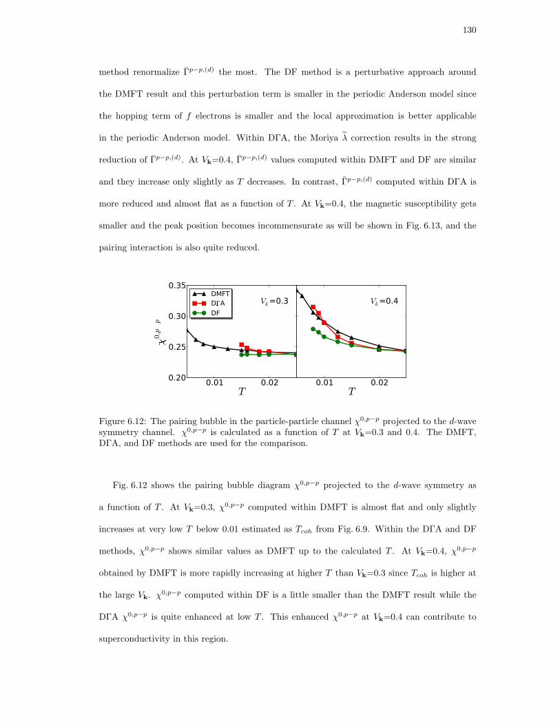
130

method renormalize Γp−p,(d) the most. The DF method is a perturbative approach around

the DMFT result and this perturbation term is smaller in the periodic Anderson model since

the hopping term of f electrons is smaller and the local approximation is better applicable

in the periodic Anderson model. Within DΓA, the Moriya λ correction results in the strong

reduction of Γp−p,(d). At Vk=0.4, Γp−p,(d) values computed within DMFT and DF are similar

and they increase only slightly as T decreases. In contrast, Γp−p,(d) computed within DΓA is

more reduced and almost flat as a function of T . At Vk=0.4, the magnetic susceptibility gets

smaller and the peak position becomes incommensurate as will be shown in Fig. 6.13, and the

pairing interaction is also quite reduced.

0.01 0.02T

0.20

0.25

0.30

0.35

R0,pSp Vk=0.3DMFTDTADF

0.01 0.02T

Vk=0.4

Figure 6.12: The pairing bubble in the particle-particle channel χ0,p−p projected to the d-wavesymmetry channel. χ0,p−p is calculated as a function of T at Vk=0.3 and 0.4. The DMFT,DΓA, and DF methods are used for the comparison.

Fig. 6.12 shows the pairing bubble diagram χ0,p−p projected to the d-wave symmetry as

a function of T . At Vk=0.3, χ0,p−p computed within DMFT is almost flat and only slightly

increases at very low T below 0.01 estimated as Tcoh from Fig. 6.9. Within the DΓA and DF

methods, χ0,p−p shows similar values as DMFT up to the calculated T . At Vk=0.4, χ0,p−p

obtained by DMFT is more rapidly increasing at higher T than Vk=0.3 since Tcoh is higher at

the large Vk. χ0,p−p computed within DF is a little smaller than the DMFT result while the

DΓA χ0,p−p is quite enhanced at low T . This enhanced χ0,p−p at Vk=0.4 can contribute to

superconductivity in this region.

131

6.2.4 The magnetic susceptibility and the spectral function

05

1015202530Um (q) Vk =0.3

T=0.015

(a) DMFTDVADF

(0,0) (W,W) (W,0) (0,0)q

05

10152025Um (q) Vk =0.4

T=0.01

(b)

Figure 6.13: The magnetic susceptibility χm(q) of the periodic Anderson model as a function ofthe momentum transfer q near TN . For comparison, χm(q) is computed from the DMFT, DΓA,and DF methods. (a) : Vk=0.3, T=0.015. In this region, the f electrons are rather localizedand the ordering vector q corresponds to 2kF of the c electrons due to the RKKY magneticinteraction. (see Fig. 6.14 (a)). (b) : Vk=0.4, T=0.01. The f electrons bahave as the itinerantquasi-particles and the ordering vector is determined from the nesting of the f electron Fermisurface. (see Fig. 6.14 (b)).

Fig. 6.13 shows χm(q) computed using the DMFT vertex function and non-local vertices

(DΓA and DF). At both Vk=0.3 and Vk=0.4, the susceptibilities calculated using non-local

methods are reduced than the DMFT susceptibility. This is due to the inclusion of non-local

correlations beyond local DMFT correlations. The DΓA susceptibility is more renormalized in

the periodic Anderson model at both Vk=0.3 and Vk=0.4. The peak position of χm(q) does

not change in both DΓA and DF methods compared to DMFT at Vk=0.4 while the DF χm(q)

peak is slightly shifted to (π − ǫ, π − ǫ) at Vk=0.3.

In the small Vk region (Vk = 0.3), the magnetic susceptibility χm(q) has a peak at q =

(π, π) as shown in Fig. 6.13(a). This peak can be understood from the spectral weight data in

Fig. 6.14(a). In this small Vk and T > Tcoh region, f electrons behave as incoherent localized

moments. As a result, Fig. 6.14(a) left shows that f electrons have the strongly reduced and

broad spectral weight in the Brillouin zone and they do not form a definite shape of the Fermi

132

XY0 YXY0Y(a) Vk =0.3,Af (k)

0.0

0.2

0.4

0.6

0.8

1.0

XY0 YXY0Y

(Z,Z)Vk =0.3,Ac (k)

0.0

0.5

1.0

1.5

2.0

XY0 YXY0Y(b) Vk =0.4,Af (k)

0

1

2

3

4

XY0 YXY0YVk =0.4,Ac (k)

0.0

0.5

1.0

1.5

2.0

Figure 6.14: The f electron and the c electron spectral function Af,c(k, ω = 0) = − 1π Gf,c(k, ω =

0). (a) The hybridization Vk=0.3ǫc and T=0.018ǫc. f electrons (left) show the broad and smallspectral weight near the Fermi energy due to incoherence (T > Tcoh) while c electrons (right)form a clear Fermi surface. (b) Vk=0.4ǫc and T=0.005ǫc. f electrons are strongly hybridizedwith c electrons and two definite Fermi surfaces are formed contributed from both f and celectrons. (T < Tcoh)

surface. In contrast, coherent c electrons show a clear circular Fermi surface. The magnetic

interaction of localized f electrons is mediated by c electrons, i.e., the RKKY interaction. In

this interaction, the magnetic ordering vector is given as 2kF of c electrons as indicated in the

white arrow of Fig. 6.14(a). This 2kF vector corresponds to the antiferromagnetic ordering

vector (π, π) of f electrons.

As Vk increases to 0.4, the χm(q) peak at q = (π, π) is strongly suppressed while the peak

position is shifted to q = (π − ǫ, π − ǫ). This peak position shift is closely related to the change

of the f electron Fermi surface. In the large Vk and small T region (T < Tcoh), f electrons are

delocalized and they form two clear Fermi surfaces as shown in Fig. 6.14(b) left. The magnetic

ordering vector (π−ǫ, π−ǫ) originates from the Fermi surface nesting vector shown as the white

arrow in Fig. 6.14(b) left. Fig. 6.14(b) right shows that c electrons are mostly concentrated on

the larger Fermi surface.

133

0.010 0.015 0.020 0.025T

2

4

6

8

Ueff

Vk=0.3

Vk=0.35

Vk=0.4

Figure 6.15: The effective U calculated as a function of T in the period Anderson model. Thedata are shown at Vk=0.3, 0.35, and 0.4. The bare interaction U is 8ǫc shown as the dashedline.

6.2.5 The effective U

Fig. 6.15 displays the effective interaction Ueff as a function of T . As Vk gets large and

T becomes small, Ueff is more renormalized since f electrons are screened by the enhanced

hybridization with c electrons. Here, Ueff is quite smaller than the bare U value even at

Vk=0.3. This implies that the screening of the periodic Anderson model is more effective due to

c electrons compared with the one-band Hubbard model with f electron alone. This screening

of Ueff originates from the scattering in the particle-particle channel known as the Kanamori

screening [92].

6.2.6 The scattering rate, ImΣ(iω = 0−)

Fig. 6.16 shows the scattering rate ImΣ(iω = 0−) result as a function of T in various Vk values.

The ImΣ(iω = 0−) value is obtained by extrapolating the lowest Matsubara points of the

DMFT ImΣ to iω = 0−. This ImΣ(iω = 0−) data can be used to determine the Tcoh of the

periodic Anderson model (see Fig. 6.9). In a Fermi liquid, the scattering rate scales as T 2 at

low T (T < Tcoh). As T increases more than Tcoh, the scattering rate increases rather slowly

and saturates at a maximum value.

134

0.00 0.02 0.04 0.06 0.08 0.10T

0.2

0.4

0.6

0.8

Im

[(i\=0])Vk =0.2

Vk =0.3

Vk =0.4

Vk =0.45

Vk =0.5

Figure 6.16: The scattering rate ImΣ(iω = 0−) as a function of T in the periodic Andersonmodel. The results are shown varying Vk from 0.2 to 0.5 values. The ImΣ data are obtainedfrom the DMFT solution.

At Vk =0.4∼0.5, ImΣ(iω = 0−) obeys this Fermi liquid behavior, i.e., it is proportional to

T 2 at low T and saturates at much higher T . Tcoh is the crossover temperature from the low T

region to the high T region. Here, we determine Tcoh as the temperature where d(ImΣ(iω=0−))dT

reaches a maximum.

In the small Vk region (Vk=0.2∼0.3), ImΣ(iω = 0−) shows strongly enhanced values at

even low T and the coherence scale below which T scales as T 2 becomes much reduced. As T

increases, the scattering rate shows a maximum and it is slowly decreased and saturated. This

maximum of ImΣ(iω = 0−) in the localized region is indicative of the resistivity maximum

at low T in the Kondo impurity model which originates from the impurity scattering with

conduction electrons. In this small Vk region, the criterion from the d(ImΣ(iω=0−))dT calculation

is ambiguous, therefore, we determine Tcoh as one half of the temperature where ImΣ(iω = 0−)

becomes maximum.

6.3 Conclusion

As a conclusion, we computed the phase diagram of the magnetic phase and the superconducting

phase in both the Hubbard model and the periodic Anderson model. In both models, the

135

superconducting phase is stable near the magnetic phase at which the magnetic fluctuation

is strong. Different vertex function calculations based on the DMFT, DF, and DΓA methods

are employed, and the results are compared. Tc is determined as a combination of the pairing

strength and the pairing bubble, i.e., the density of states of the system. The SC gap function

is closely related to the momentum dependence of the pairing vertex and the Fermi surface

geometry of quasi-particles.

The vertex function calculation based on DMFT, DF, and DΓA is an inexpensive and

efficient approach to compute Tc and the SC gap symmetry compared to the cluster extension

of DMFT. We showed that these approaches can capture the strong magnetic fluctuation effect

causing the pairing instability in both the Hubbard model and the periodic Anderson model. As

shown in Chapter 4, this vertex function approach can be applied to the realistic multi-orbital

system in a straightforward way. The cluster DMFT is not applicable to the multi-orbital

system since it gets numerically too expensive. The RPA calculation of superconductivity is

quite inexpensive but it works exclusively in the itinerant limit, and the irreducible vertex in

the particle-hole channel is replaced by a constant as an approximation. Therefore, the vertex

function calculation approach will be a promising route to study the microscopic origin of the

pairing mechanism in many superconducting correlated materials.

136

Chapter 7

The Magnetic Excitation Spectra in Fe-based

Superconductors

In this chapter, we study the magnetic excitation spectra in the paramagnetic state of BaFe2As2

from the ab initio perspective [77]. The one-particle excitation spectrum is determined within

the combination of the density functional theory and the dynamical mean-field theory method.

The two-particle response function is extracted from the local two-particle vertex function, also

computed by the dynamical mean field theory, and the polarization function. This method

reproduces all the experimentally observed features in inelastic neutron scattering (INS), and

relates them to both the one particle excitations and the collective modes. At low frequency the

magnetic excitation spectra, as encoded in S(q, ω), is strongly peaked at the magnetic ordering

wave vector (1, 0, 1). With increasing energy the peak position shifts, and around 230meV the

peak moves to the wave vector (1, 1, 1), in good agreement with inelastic neutron scattering

(INS) experiments on BaFe2As2. This high energy peak is shown to originate mainly from

the intra-orbital excitations in the dxy orbital from the momentum space regions near the two

electron pockets. The magnetic excitation dispersion is well accounted for by our theoretical

calculation in the paramagnetic state without any broken symmetry, hence nematic order is not

needed to explain the INS experimental data.

137

7.1 Introduction to Fe-based superconductors

7.1.1 History

In 2008, Hideo Hosono and the co-workers discovered that fluorine-doped LaOFeAs shows su-

perconductivity with as high Tc as 26K [97]. Right after this discovery, it was reported that

fluorine-doped LaOFeAs can show Tc around 43K by the application of pressure [98] and the

Tc value can be further increased by replacing La by other rare earth elements [99]. Following

this discovery of the Fe-based superconductor, tremendous research efforts have been stimulated

to synthesize new Fe-based compounds with higher Tc and to understand the origin of super-

conductivity in these new materials. After the experimental discovery, theoretical electronic

structure calculation [70] showed that these materials have both localized and itinerant aspects

of correlated electrons, and the pairing mechanism of superconductiviy can be non-phonon me-

diated similar as the cuprate superconductors. However, it is not unraveled until now what is

really the mediator of pairing in these systems and it requires new theoretical advances and

experimental efforts. Therefore, the discovery of the Fe-based superconductors has opened a

new avenue of research to understand the origin of superconductivity in strongly correlated

condensed matter systems.

7.1.2 Crystal structure

The crystal structure of Fe-based superconductors has a common feature, i.e., it has a lay-

ered structure based on Fe atoms joined by tetrahedrally coordinated pnictogens (P, As) or

chalcogens (S, Se, Te). And these layers are arranged in a stacked sequence separated by alkali,

alkaline-earth or rare-earth and oxygen/fluorine layers. The Fe-based superconductors with Fe

atoms surrounded by pnictogens are usually called as Fe pnictides and the materials with Fe

atoms surrounded by chalcogens are called as Fe chalcogenides. Similar to the CuO2 plane in

cuprate superconductors, the two-dimensional Fe plane plays an important role for magnetism

and superconductivity in these materials.

138

Figure 7.1: The crystal structure of BaFe2As2. This figure depicts the conventional unit cell ofthe body-centered tetragonal structure.

The five distinct tetragonal structures are known to exist in Fe-based superconductors [4].

Fig. 7.1 shows the body-centered tetragonal structure of BaFe2As2, so called the 122 structure.

This structure is the most studied one among the five structures. The known experimental

lattice constants for BaFe2As2 are shown in Table. 7.1. The large c/a ratio indicates that

two-dimensional physics may be crucial for the study in 122 systems. Moreover, zAs plays an

crucial role in determining Tc of Fe-based superconductors and Tc is highest when the As-Fe-As

tetrahedral bond angle is closest to the ideal value of 109.47

a 3.9625A

c 13.0168A

zAs 1.3603A

Table 7.1: The lattice constants of BaFe2As2. a is the length in the x- (y-) direction of theconventional unit cell, c is the height of the unit cell, and zAs is the height of the As atom fromthe Fe plane.

139

7.1.3 Phase diagram

Figure 7.2: The phase diagram of BaFe2As2 obtained by the chemical substitution of either Bawith K [1] (dark blue), Fe with Co [2] (blue), or As with P [3] (red). The dashed line shows thestructural transition. This figure is taken from Ref. [4].

Fig. 7.2 displays the phase diagram of BaFe2As2 obtained by manipulating the chemical

doping/substitution of the material. By substituting either the alkaline-earth (Ba), transition-

metal (Fe), or pnictogen (As) atom with a different element, one can produce the similar

phase diagrams once the chemical substitution is normalized to overlap the descent of the

AFM transition. The chemical substitution or alternatively applied external pressure drives an

antiferromagnetic (AFM) state to a superconducting (SC) state. Between the AFM and the SC

states, two states also coexist within a certain range. A structural phase transition from the

tetragonal (T) structure to the orthorhombic (O) phase is observed for Co substitution, which

is coincident with the paramagnetic to AFM phase transition in BaFe2As2. This phase diagram

of iron pnictide is quite similar with the phase diagram of cuprates. However, a significant

difference is the AFM state of the parent compound in BaFe2As2 is metallic while the parent

compound of cuprates shows the Mott insulating behavior. Due to the metallic nature of

magnetism in iron pnictides, it is crucial to understand whether magnetism in these materials

140

can be described with either the localized picture or the itinerant picture, or both pictures are

required.

7.1.4 Inelstic neutron scattering in Fe-based superconductors

Neutron scattering [100] is a powerful experimental technique since it sheds light on studying

the magnetic structure and dynamics of condensed matter system. A neutron has zero chage

and hence it does not interact with other charged particles such as an electron or a proton by

the Coulomb interaction. Therefore, a neutron can penetrate deeply into a material and it can

measure the bulk property. However, a neutron has one half spin, therefore it readily interacts

with the magnetic moment of an electron by the dipole-dipole interaction.

Since neutron scattering acts as a weak perturbation to the system, the differential cross

section can be calculated from the Fermi Golden rule. In inelastic neutron scattering (INS), the

differential cross section is given by

d2σ

dΩdE=

kf

ki(

mN

2π~2)2| 〈kfλf |V |kiλi〉 |2δ(~ω + Ei − Ef ) (7.1)

where V is the interaction operator for the neutron, λi(f) is the quantum numbers for ini-

tial(final) state of the sample, ki(f) is initial(final) momentum, Ei(f) is the initial(final) energy,

and mN is the neutron mass. The magnetic field generated inside matter can be produced by

either the electron spin or the electron orbital motion. Here, we consider only the contribu-

tion from the electron spin. A neutron interacts with this electron spin by the dipole-dipole

interaction. Therefore, the magnetic interaction V is given by

V = −µN · B = −µ0µN

4π[∇× (

µe × R

R2)] (7.2)

Here, µ0 is the magnetic constant, µe is the electron magnetic moment, and µN is the neutron

magnetic moment.

By inserting Eq. 7.2 to Eq. 7.1, the magnetic cross section is given by

d2σ

dΩdE= (γr0)

2Nkf

ki· f(q)2 · e−2W

∑

αβ

(δαβ − qα · qβ) · Sαβ(q, ω) (7.3)

141

where α, β means the coordinates (x, y, z) and δαβ − qα · qβ term means only the magnetic

moment perpendicular to q contributes to the cross section. And f(q) is the magnetic form

factor obtained by the Fourier transform of the unpaired electron density. Here, S(q, ω) is the

dynamical structure factor which is the Fourier transform of the spin-spin correlation function

and given by

Sαβ(q, ω) =1

2π~

∫dte−iωt

∑

l

eiq·rl

⟨Sα

0 (0) · Sβl (t)

⟩. (7.4)

Due to the fluctuation-dissipation theorem, the imaginary part of the magnetical susceptibility

is related to the correlation funciton by the following equation

S(q, ω) =χ′′(q, ω)

1 − e−~ωkT

. (7.5)

Neutron scattering experiments provide strong constraints on the theory of iron pnictides.

Both the localized picture and the itinerant picture of the magnetic response have had some suc-

cesses in accounting or even predicting aspects of the experiments. Calculations based on a spin

model with frustrated exchange constants [101, 102] or with biquadratic interactions [103] de-

scribed well the neutron scattering experiments [104, 105]. The itinerant magnetic model, based

on an random phase approximation (RPA) form of the magnetic response, uses polarization func-

tions extracted from density functional theory (DFT) [106] or tight binding fits [107, 81, 108]

and produces equally good descriptions of the experimental data.

Furthermore, DFT calculations predicted the stripe nature of the ordering pattern [109] and

the anisotropic values of the exchange constants which fit well the spin wave dispersion in the

magnetic phase [110]. The tight binding calculations based on DFT bands also predicted the

existence of a resonance mode in the superconducting state [111].

In spite of these successes, both itinerant and localized models require significant exten-

sions to fully describe the experimental results. DFT fails to predict the observed ordered

moment [110]. Furthermore, adjusting parameters such as the arsenic height to reproduce the

ordered moment, leads to a peak in the density of states at the Fermi level [106], instead of

the pseudogap, which is observed experimentally. The localized picture cannot describe the

142

magnetic order in the FeTe material without introducing additional longer range exchange con-

stants. Given that this material is more localized than the 122, the exchange constants would

be expected to be shorter range. Furthermore, fits of the INS data require the use of anisotropic

exchange constants well above the magnetic ordering temperature [5]. However no clear phase

transition to a nematic phase in this range has been detected.

In this chapter, we argue that the combination of density functional theory and dynamical

mean field theory (DFT+DMFT) provides a natural way to improve both the localized and the

itinerant picture, and connects the neutron response to structural material specific information

and to the results of other spectroscopies.

7.2 Calculation methods

7.2.1 The dynamical magnetic susceptibility χ(q, ω)

In this subsection, we explain the method for computing the dynamical magnetic susceptibility

χ(q, ω) using a combination of density functional theory (DFT) and dynamical mean field theory

(DMFT). The equations for computing χ(q, iω) are already derived in Section 4.4 in details.

Therefore, we explain here how to compute χ(q, iω) briefly and discuss how to analytically

continue the obtained χ(q, iω) to χ(q, ω) on the real axis.

Within DFT+DMFT, the dynamical magnetic susceptibility χ(q, iω) is computed from the

ab initio perspective using the polarization bubble χ0 and the two-particle irreducible vertex

function Γirrloc of DFT+DMFT solution [112], which is assumed to be local in the same basis

in which the DMFT self-energy is local, implemented here by the projector to the muffin-tin

sphere [14]. χ0 is computed from the fully interacting one particle Greens function. We compute

the one-particle Green’s function using the charge self-consistent full potential DFT+DMFT

method, as implemented in Ref. [14], based on Wien2k code [113]. We used the continuous-time

quantum Monte Carlo (CTQMC) [17, 16] as the quantum impurity solver, and the Coulomb

interaction matrix as determined in Ref. [114]. (U=5eV and J=0.7eV respectively) In order to

143

extract Γirrloc , we employ the Bethe-Salpeter equation which relates the local two-particle Green’s

function (χloc), sampled by CTQMC, with both the local polarization function (χ0loc) and Γirr

loc :

Γirrloc α1σ1,α2σ2

α3σ3,α4σ4

(iν, iν′)iω = [(χ0loc)

−1iω − χ−1

loc]. (7.6)

Γirrloc depends on three Matsubara frequencies (iν, iν′; iω), and both the spin (σ1−4) and the

orbital (α1−4) indices, which run over 3d states on the iron atom.

The momentum dependent two-particle Green’s function χ is constructed using the Bethe-

Salpeter equation by replacing the local polarization function χ0loc by the non-local one χ0

q,iω:

χα1σ1,α2σ2α3σ3,α4σ4

(iν, iν′)q,iω = [(χ0)−1q,iω − Γirr

loc ]−1. (7.7)

Finally, the dynamic magnetic susceptibility χ(q, iω) is obtained by closing the two particle

green’s function with the magnetic moment µ = µB(L+2S) vertex, and summing over frequen-

cies (iν,iν′), orbitals (α1−4), and spins (σ1−4) on the four external legs

χ(q, iω) =∑

iν,iν′

∑

α1α2α3α4

∑

σ1σ2σ3σ4

µzα1σ1α3σ3

µzα2σ2α4σ4

χα1σ1,α2σ2α3σ3,α4σ4

(iν, iν′)q,iω (7.8)

The resulting dynamical magnetic susceptibility is obtained in Matsubara frequency (iω)

space and it needs to be analytically continued to real frequencies (χ(q, ω)) in order to compare

with the INS data. For the low frequency region, on which we concentrate here, the vertex

Γirrloc is analytically continued by a quasiparticle-like approximation. We replace the frequency

dependent vertex with a constant, i.e.,

Γirrloc α1σ1,α2σ2

α3σ3,α4σ4

(iν, iν′)iω ≈ Uα1σ1,α2σ2α3σ3,α4σ4

(q) (7.9)

and require χ(q, iω = 0) = χ(q, ω = 0). This vertex U however retains important spin and

orbital dependence. And U acquires even the weak momentum q dependence to satisfy the

above condition.

The analytic continuation of the one-particle Green’s function to the real axis is achieved

by analytically continuing the self energy using the method implemented in Ref. [14]. Since the

144

two-particle vertex is approximated to a frequency independent constant on the real axis, the

internal Matsubara frequency iν of the polarization bubble χ0 can be summed over:

χ0αβδγ

(q, iω) = − 1

Nk

∑

k,iν

Gαβ(k, iν) · Gγδ(k + q, iν + iω)

= − 1

Nk

∑

k

1

2πi

∮dzGαβ(k, z) · Gγδ(k + q, z + iω)

= − 1

Nk

∑

k

∫dν [Aαβ(k, ν) · Gγδ(k + q, ν + iω) − Gαβ(k, ν − iω) · Aγδ(k + q, ν)]

·f(ν) (7.10)

where f(ν) is the Fermi function. Here, we replace the Matsubara sum to the integral over the

complex plane. And χ0 can be obtained on the real axis:

(χ0)′′αβδγ

(q, ω) = − π

Nk

∑

k

∫dν[Aαβ(k, ν) · Aγδ(k + q, ν + ω) − Aαβ(k, ν − ω) · Aγδ(k + q, ν)]f(ν)

= − π

Nk

∑

k

∫dνAαβ(k, ν) · Aγδ(k + q, ν + ω) · [f(ν) − f(ν + ω)] (7.11)

Here, (χ0)′′(q, ω) ≡ 12i [χ

0(q, ω+iδ)−χ0(q, ω+iδ)] and A(k, ν) ≡ 12πi [G(k, ν+iδ)−G(k, ν−iδ)].

The real part of χ0 can be computed using the Kramers-Kronig relation from (χ0)′′.

The two-particle Green’s function χαβγδ

(q, ω) is computed using χ0(q, ω) and U by the fol-

lowing Bethe-Salpeter equation

χασαβσβγσγ δσδ

(q, ω) = χ0ασαβσβγσγ δσδ

(q, ω) +∑

ηµλν

∑

σησµσλσν

χ0ασαησηγσγ λσλ

(q, ω) · U ησηµσµλσλνσν

(q) · χµσµβσβνσν δσδ

(q, ω) (7.12)

Finally, the magnetic susceptibility χ(q, ω) is obtained by closing the four external legs with

the magnetic moment µ = µB(L + 2S) vertex by summing orbitals (α1−4) and spins (σ1−4) in

a similar way as Eq. 7.8, i.e.,

χ(q, ω) =∑

α1α2α3α4

∑

σ1σ2σ3σ4

µzα1σ1α3σ3

µzα2σ2α4σ4

χα1σ1,α2σ2α3σ3,α4σ4

(q, ω) (7.13)

For the analytic continuation of χ(q, iω) to the real axis, we approximated Γirr to U as shown

in Eq. 7.9. This approximation ensures that χ(q, ω = 0) value is always exact to χ(q, iω = 0)

within vertex calculation since U is determined to satisfy this condition. In order to check how

this approximation is reliable at finite frequencies, we compare χ(q, iω) computed from Γirr

using Eq. 7.7 with χU (q, iω) obtained from the approximated U .

145

0

1

2

3

4

5

6^(i_) Local

const U

Vertex

(H,K,L)=(0,0,1)

0.0 0.2 0.4 0.6 0.8i [eV]

0

1

2

3

4

5^(i_) (H,K,L)=(1,0,1)

0.0 0.2 0.4 0.6 0.8 1.0i [eV]

(H,K,L)=(1,1,1)

Figure 7.3: The comparison between χ(q, iω) (red triangle) computed using vertex functionΓirr and χU (q, iω) (black circle) obtained by U . Both quantities are given on the five lowestMatsubara frequencies and at distinct wave vectors q=(0,0,1), (1,0,1), and (1,1,1) and for thelocal value.

Fig 7.3 shows both χ(q, iω) (red triangle) and χU (q, iω) (black circle) at q=(0,0,1), (1,0,1),

and (1,1,1) and for the local value. χU (q, iω) values are slightly smaller than χ(q, iω) values

except for q=(0,0,1) where both values are almost the same. This is because the approximated U

is estimated for ω=0 and the value is more renormlized compared to the vertex at high frequency

ω. The discrepancy between χ(q, iω) and χU (q, iω) is pronounced at q=(1,0,1) especially at

the second and the third iω points, however, χU (q, iω) values show an overall good agreement

with χ(q, iω) values.

7.2.2 The phase factor for one Fe atom per unit cell

The primitive unit cell of BaFe2As2 contains two Fe atoms due to two nonequivalent positions

of As atoms. Since almost entire magnetic moment is concentrated on Fe atoms, which form

a square lattice, the inelastic neutron scattering (INS) data should be compared to calculation

of magnetic susceptibility in the large Brillouin zone coming from this square lattice. This

is because the folding of the bands is noticeable only in those quantities which have finite

146

contribution from the As atoms. Therefore, we computed the dynamical magnetic susceptibility

within DFT+DMFT in this large Brillouin zone.

Due to inequivalent As atoms within a unit cell, the naive projection to orbital basis does

not results in correct translational symmetry between Fe atoms within the unit cell. Let us

consider a tight-binding Hamiltonian, written in some orbital basis, i.e.,

Hατ,α′τ ′(R,R′) = 〈ϕατ (r + R)|H|ϕα′τ ′(r + R′)〉. (7.14)

Here, τ goes over the two Fe sites in the unit cell, which we label by a sublattice A and a

sublattice B. α is the orbital index. This Hamiltonian does not have the required transla-

tional symmetry Hατ,α′τ ′(R,R′) 6= Hα,α′,τ−τ ′(R,R′). However, we can restore the translational

symmetry by choosing a different wave function on each sublattice, such that the new basis

function on sublatice A is φAα (r) ≡ ϕα(x, y, z) and on sublattice B is φB

α (r) ≡ ϕα(x, y,−z).

This is because the As atom is positioned above the Fe plane in A sublattice and below the

iron plane in B sublattice, hence the local environment on Fe atom looks translational invariant

only in this new φα orbital basis. Consequently, the tight-binding Hamiltonian expressed in φα

basis in translationally invariant.

Our DFT+DMFT implementation does not require construction of tight-binding Hamilto-

nians, but it rather employs the projection technique. The projection matrix PK(i, j; τ, α, τ ′α′)

project physical quantities, such as the Green’s function, written in Kohn-Sham basis in terms of

bands |i, j〉 and the momentum K, to a local orbital subspace |τα, τ ′α′〉(see Eq.12 in Ref. [14]).

By adopting the different local orbital basis for τA and τB as mentioned in the previous para-

graph, this projection matrix defined for two Fe atoms per unit cell can restore the translational

symmetry for one Fe atom per unit cell.

The projection matrix Pk(i, j;α, α′) in one Fe atom per unit cell acquries the phase factor

that modulates with the internal vectors (τ) within the unit cell in addition to PK(i, j; τ, α, τ ′α′).

In one Fe atom per unit cell, the momentum k is defined in the unfolded Brillouine zone (BZ)

due to the smaller unit cell. The detailed derivation is given as the following equations using

several unitary transformations with the real space basis (|R〉). A similar derivation is used in

147

the previous literature [115].

〈k, α|K, i〉 ∼=∑

Rτα′

〈k, α|R, τ, α′〉 〈R, τ, α′|K, i〉 =1

NR

√Nτ

∑

Rτα′

e−ik·(R+τ)δαα′eiK·R 〈τ, α′|K, i〉

=1√Nτ

∑

τ

δk,[K]e−ik·τ 〈τ, α|K, i〉 (7.15)

Pk(i, j;α, α′) = 〈k, α|K, i〉 〈K, j|k, α′〉 =1

Nτ

∑

ττ ′

δk,[K]e−ik·(τ−τ ′) 〈τ, α|K, i〉 〈K, j|τ ′, α′〉

=1

Nτ

∑

ττ ′

δk,[K]e−ik·(τ−τ ′)PK(i, j; τα, τ ′α′) (7.16)

Here, K(k) is the momentum in the (un)folded Brillouin zone, [K] means the set of momentum

vectors which are equivalent to K by the modulo of the reciprocal vector G. i, j are the band

indices, R is the lattice vector for a primitive unit cell (two Fe per cell), τ is the internal vector

within the unit cell, α is the local orbital basis defined inside the Fe atom, and Nτ is the number

of Fe atoms inside the unit cell.

The spectral quantities which are mostly concetrated on the Fe atoms can be computed in

the symmetry of one Fe atom per unit cell using this projection matrix (Eq.7.16). For example,

the Green’s function projected to one Fe atom per unit cell can be given by

Gαβ(k, ν) =∑

K,i,j

gij(K, ν) · Pk(i, j;α, β) (7.17)

where gij =(

1ν+µ−ǫK−P−1Σ

)ij

is the Green’s function on the band indices.

7.3 Magnetic excitation spectra in BaFe2As2: DFT+DMFT results

7.3.1 The dynamical structure factor S(q, ω) results

Fig. 7.4(a) shows the calculated constant energy plot of the dynamical structure factor, S(q, ω)

in the paramagnetic state of BaFe2As2. Our theoretical results are calculated in the unfolded

Brillouin zone of one Fe atom per unit cell, because magnetic excitations are concentrated

primarily on Fe atoms, therefore folding, which occurs due to the two inequivalent arsenic atoms

in the unit cell, is not noticeable in magnetic response [107]. For comparison we also reproduce

in Fig. 7.4(b) the INS experimental data from Ref. [5]. At low energy (around ω=50meV),

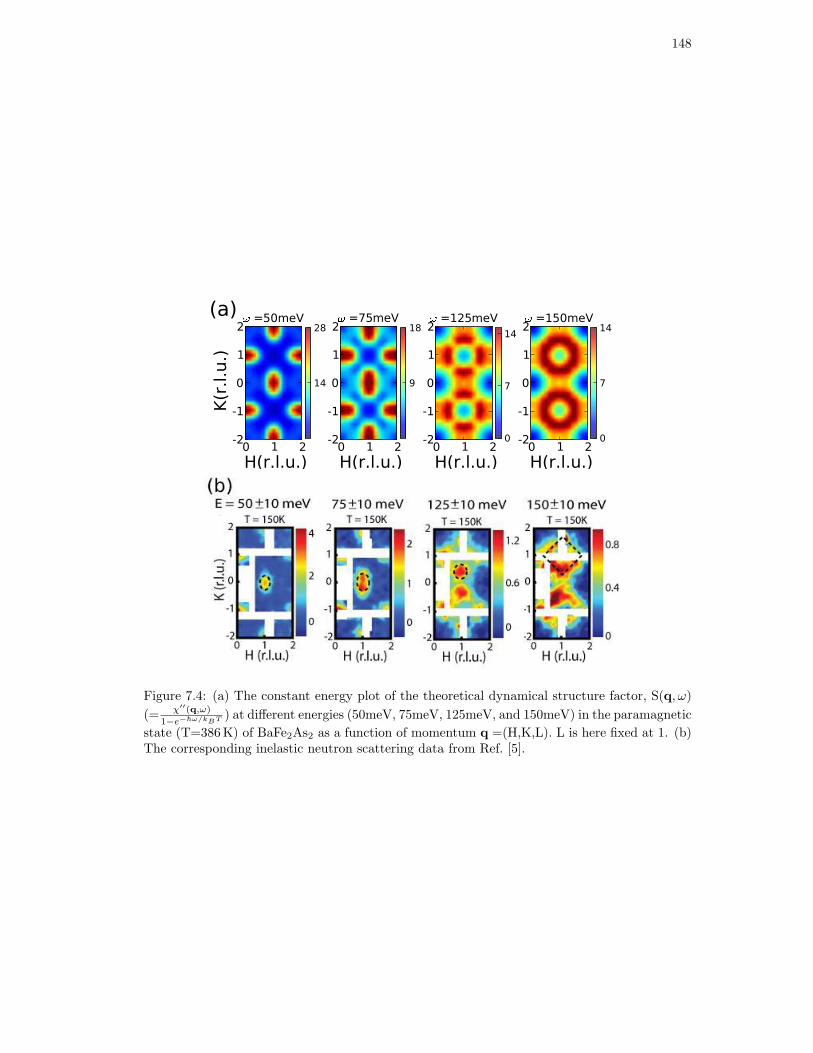
148

0 1 2

H(r.l.u.)

-2

-1

0

1

2

K(r

.l.u

.)

(a)a =50meV

14

28

0 1 2

H(r.l.u.)

-2

-1

0

1

2a =75meV

9

18

0 1 2

H(r.l.u.)

-2

-1

0

1

2a =125meV

0

7

14

0 1 2

H(r.l.u.)

-2

-1

0

1

2a =150meV

0

7

14

Figure 7.4: (a) The constant energy plot of the theoretical dynamical structure factor, S(q, ω)

(= χ′′(q,ω)

1−e−~ω/kBT ) at different energies (50meV, 75meV, 125meV, and 150meV) in the paramagnetic

state (T=386K) of BaFe2As2 as a function of momentum q =(H,K,L). L is here fixed at 1. (b)The corresponding inelastic neutron scattering data from Ref. [5].

149

the theoretical S(q, ω) is strongly peaked at the ordering wave vector (H,K,L)=(1, 0, 1) and it

forms a clear elliptical shapes elongated in K direction. The elongation of the ellipse increases

with energy (ω=75meV) and around ω =125meV the ellipse splits into two peaks, one peak

centered at (1, 0.4, 1) and the other at (1,−0.4, 1). At even higher energy (ω ≈150meV) the

magnetic spectra broadens and peaks from four equivalent wave vectors merge into a circular

shape centered at wave vector (1, 1, 1). At even higher energy (230meV, not shown in the figure)

the spectra broadens further, and the peak becomes centered at the point (1, 1, 1). These trends

are all in good quantitative agreement with INS data from Fig. 7.4(b).

(0,0) (1,0) (1,1) (0,0)(H,K) [r.l.u]

0

100

200

300

400

b [meV]

0

2

4

6

8

10

12

14

16

18

Figure 7.5: S(q, ω) along the special path in Brillouin zone marked by red arrow in the inseton the right. The inset shows the body-centered tetragonal (black line) and the unfolded (blueline) Brillouin zone. Black dots with error bars correspond to INS data from Ref. [5]. The whitedashed line shows the isotropic Heisenberg spin wave dispersion.

In Fig. 7.5, we display a contour plot of the theoretical S(q, ω) as a function of frequency ω

and momentum q along the special path in the unfolded Brillouin zone, sketched by a red line in

the right figure. At low energies (ω <80meV), S(q, ω) is mostly concentrated in the region near

the ordering vector (1, 0, 1). Consistent with the elongation of the ellipse along the K direction

in Fig.7.4, the low energy (ω <80meV) bright spot in Fig.7.5 is extended further towards (1, 1, 1)

150

direction but quite abruptly decreases in the (0, 0, 1) direction. The magnetic spectra in the two

directions (1, 0, 1) → (0, 0, 1) and (1, 0, 1) → (1, 1, 1) are clearly different even at higher energy

ω > 100meV. The peak position is moving to higher energy along both paths, but it fades away

very quickly along the first path, such that the signal practically disappears at (0.5, 0, 1). Along

the second path (1, 0, 1) → (1, 1, 1), there remains a well defined excitation peak for which the

energy is increasing, and at (1, 1, 1) reaches the maximum value of ≈ 230meV. Continuing the

path from (1, 1, 1) towards (0, 0, 1) the peak energy decreases again and it fades away around

(0.5, 0.5, 1). The black dots display INS data with errors bars from Ref. [5]. Notice a very good

agreement between theory and experiment.

The white dashed line in Fig.7.5 represents the spin wave dispersion obtained for the isotropic

Heisenberg model using nearest neighbor J1 and next nearest neighbor J2 exchange constants

and performing the best fit to INS data. This fit was performed in Ref. [5]. The magnetic

excitation spectra of an isotropic Heisenberg model show a local minimum at the wave vector

q = (1, 1, 1), which is inconsistent with our theory and with the experiment. To better fit the

experimental data with a Heisenberg-like model, very anisotropic exchange constants need to

be assumed [5], which raised speculations about possible existence of nematic phase well above

the structural transition of BaFe2As2. Since the DFT+DMFT results can account for all the

features of the measured magnetic spectra without invoking any rotationally symmetry breaking

the presence of nematicity in the paramagnetic tetragonal state at high temperature is unlikely.

In Fig. 7.6(a) we show constant frequency cuts in the K direction (from (1,−1, 1) through

(1, 0, 0) to (1, 1, 1)) of S(q, ω) displayed in Fig. 7.5. For comparison we also show the corre-

sponding INS measurements from Ref. [5] as red circles in Fig. 7.6(b) and (c). At ω=20meV,

the spectrum has a sharp peak centered at the ordering vector (1, 0, 1). At ω=50meV, the spec-

trum still displays a peak at (1, 0, 1) but the intensity is significantly reduced. With increasing

frequency ω, the peak position in S(q, ω) moves in the direction of (1, 1, 1), and at 128meV

peaks around (1, 0.4, 1). The shift of the peak is accompanied with substantial reduction of

intensity at ordering wave vector (1, 0, 1). At even higher energy of 250meV only a very weak

151

c1.0 c0.5 0.0 0.5 1.0K [r.l.u]

S(q

,

d)(arb.units) H=1

L=1(a) e=20meVe=50meVe=128meVe=250meV

Figure 7.6: (a) The wave vector K dependence (H=1,L=1) of S(q, ω) at several frequencies. (b)The corresponding INS data at ω=19meV and (c) 128meV reproduced from Ref. [5]. The redcircles correspond to the paramagnetic state at T=150K and the blue diamonds to the magneticstate at T=7K.

peak remains, and it is centered at the wave vector (1, 1, 1). The position of peaks as well as

their frequency dependence is in very good agreement with INS experiments of Ref. [5] displayed

in Fig. 7.6(b) and (c).

7.3.2 The d orbital resolved χ(q, ω)

Fig. 7.7(a) resolves the dynamical magnetic susceptibility χ of Eq. 7.8 in the orbital space

χα = T∑

iν,iν′

∑β

∑σ1σ2σ3σ4

µzσ1σ3

µzσ2σ4

χασ1,βσ2ασ3,βσ4

(iν, iν′) such that χ =∑

α χα. At the magnetic

ordering vector q=(1, 0, 1), χ′′

α increases sharply with frequency near ω = 0 for all orbitals and is

strongly suppressed above 100meV reaching the maximum around 20meV. At this wave vector,

the dominant contributions at low energy come from the dxy and the dyz orbitals. The magnetic

susceptibility at q=(0, 1, 1) in Fig. 7.7(a) shows the same trend as orbitally resolved spectra at

q=(1, 0, 1), except that dxz and dyz switch their roles due to the C4 symmetry of the Fe square

lattice. Magnetic excitation spectra at q=(0,0,1) and q=(1,1,1) show the noticeable difference.

152

fgg(q,h)(arb.unit

s)

(a)(H,K,L)=(1,0,1) (H,K,L)=(0,1,1)

0 100 200 300 400i [meV]

fgg(q,h)(arb.unit

s)

(H,K,L)=(0,0,1)z2

x2 -y2

xzyzxy

0 100 200 300 400 500i [meV]

(H,K,L)=(1,1,1)

0.0

0.1

0.2

Im

j0(q,k) DFT+DMFT(H,K,L)=(1,0,1)

(b)z2

x2 -y2

xzyzxy

(H,K,L)=(0,1,1)

0 100 200 300 400l [eV]0.0

0.1

0.2

Im

j0(q,k) (H,K,L)=(0,0,1)

0 100 200 300 400 500l [eV]

(H,K,L)=(1,1,1)

Figure 7.7: (a) The Fe d orbital resolved dynamical magnetic susceptibility χ(q, ω) at T=386Kfor distinct wave vectors q=(1, 0, 1), (0, 1, 1), (0, 0, 1), and (1, 1, 1). Different colors correspondto different orbital contributions. (b) The Fe d orbital resolved polarization bubble χ0(q, ω) atthe same T and the same wave vectors q as (a)

153

These wave vectors are at the center of the lattice C4 symmetry, therefore, the spectra from the

dxz orbital and the dyz orbital are always degenerate. At q=(0,0,1), dxz, dyz, and dxy orbitals

are mostly contributed to low energy while high energy excitations are strongly suppressed at all

d orbitals. In contrast, q=(1,1,1) the excitation spectra at q=(1,1,1) show only slight increase

at low energy while the high energy spectra are peaked near 230meV for all orbitals but with

the large dxy contribution.

Fig. 7.7(b) displays the orbital resolved χ0 calculated at the same q vectors as (a). The

dominant orbital contributions to χ shown in (a) are also reasonably captured in the polarization

bubble χ0. At q=(1, 0, 1), the dxy and the dyz orbitals show the large spectra compared to other

orbitals increasing almost linearly at low energy. At q=(0, 1, 1), the dxy and the dxz orbitals

show the enhanced spectra. Other orbitals are strongly suppressed at low energy and they are

increasing with a slow rate. At q=(0, 0, 1), the dxy, the dxz, and the dyz orbitals have large

spectral weights showing the peak near 100meV. The dz2 and the dx2−y2 orbitals show the

negligible contribution. At q=(1, 1, 1), all d orbitals exhibit strongly suppressed spectra at low

energy and increases slowly even at higher energies. Only dxy orbital shows a quite enhanced

spectra around 350-400meV and this peak can be attributed to the intra-orbital excitation

between dxy bands as will be shown in Fig. 7.8(b). One can note that the full χ at q=(1, 1, 1)

has the peak at the smaller energy around 230meV due to strong correlations treated by the

irreducible vertex function Γirr. These different orbital contributions to χ0 can be understood

from the orbital resolved Fermi surface and the spectral function as will be shown below.

7.3.3 The d orbital resolved Fermi surface

The orbital resolved Fermi surface is displayed in Fig. 7.8(a) at both the Γ-plane and the Z-

plane. Most of the weight in χ0 shown in Fig. 7.7(b) comes from the diagonal terms, i.e., χ0α,α,

hence the Fermi surfaces with the same color in Fig. 7.8(a) but separated by the wave vector

(1, 0, 1) give dominant contribution. The intra-orbital dyz low energy spectra comes mostly

from the transitions between the green parts of the hole pocket at Γ and the green parts of the

154

0 1H(r.l.u.)

0

1

K(r.l.u.)

mn(a)

oM

Mp X

L=0

0 1H(r.l.u.)

qrZ A

Ap R

L=1

s tu v-0.4

-0.2

0

0.2xy

yz xy

xz

(b)

Figure 7.8: (a) The Fermi surface in the Γ and Z plane at T=73K colored by the orbitalcharacters: dxz(blue), dyz(green), and dxy(red). The small symbols mark the regions in theFermi surface, where nesting for the wave vector q=(1, 0, 1) is good. (b) The zoom-in of A(k, ω)along the path marked by black dashed line in Fig. 7.8(a). The green open circles indicate thetwo relevant bands of dxy character which give rise to the peak in magnetic excitation spectranear 230meV at q=(1, 1, 1).

155

electron pocket at A, marked with green squares (¤) in Fig. 7.8(a). Since the electron pocket

at A is elongated in H direction, the nesting condition occurs mostly in the perpendicular K

direction, hence the elliptical excitations at low energy in Fig. 7.4 are elongated in K but not

in H direction. The intra-orbital dxy transitions are pronounced between the electron pocket at

M ′ and the hole pocket at R, as well as between the electron pocket at A′ and the hole pocket

at X (marked with red ©). This large spin response at (1, 0, 1) gives rise to the low energy

peak in Fig. 7.5.

We note that the particle-hole response, encoded in polarization bubble χ0, is especially

large when nesting occurs between an electron pockets and a hole pocket, because the nesting

condition extends to the finite frequency, and is not cut-off by the Fermi functions.

The low energy magnetic excitations at wave vectors q = (0, 0, 1) and q = (1, 1, 1) can come

only from electron-electron or hole-hole transitions, hence both responses are quite small, as

seen in Fig. 7.7(a). While the magnetic response at q = (0, 0, 1) is small but finite, the spin

response at q = (1, 1, 1) is almost gapped. This is because the hole-hole transitions from Γ to R

or electron-electron transitions from M to A′ do not involve any intra-orbital transitions, and

hence are even smaller than transitions at the wave vector (0, 0, 1).

At finite energy transfer, the spin excitations come from electronic states away from the

Fermi energy, and can not be easily identified in the Fermi surface plot. Hence it is more

intriguing to find the dominant contribution to the peak at ω ≈ 230meV and q = (1, 1, 1).

This peak gives rise to the 230meV excitations at (1, 1, 1) in Fig. 7.5. A large contribution to

this finite frequency excitation comes from a region near the two electron pockets at M and A′

marked with black dashed line in Fig. 7.8(a). We display in Fig. 7.8(b) the one electron spectral

function across these dashed lines in the Brillouin zone to show an important particle hole

transition from the electrons above Fermi level at the M point and the flat band at -200meV

around the A′ point, both of dxy character. We note that due to large off diagonal terms in the

two particle vertex Γ, all orbital contributions to χ develop a peak at the same energy, although

only dxy orbital displays a pronounced peak in χ0.

156

7.3.4 Spectral function

wM X wZ A R Z-0.6

-0.4

-0.2

0

0.2

xy

xy

xy

xy

Figure 7.9: A(k, ω) computed in one Fe atom per unit cell at T=73K. The green arrows markthe same bands which give rise to 230meV peak. The DFT bands are overlayed by white dashedlines. The blue arrows mark corresponding DFT bands of dxy character.

Fig. 7.9 displays the one electron spectral function in a path through the Brillouin zone,

corresponding to one Fe atom per unit cell. Within DFT+DMFT the quasi-particle bands are

renormalized by a factor of 2-3 compared to the corresponding DFT bands (white dashed lines).

The green arrow marks the dxy band which contributes to the peak in S(q, ω) near 230meV and

q = (1, 1, 1). In DFT calculation, this dxy intra-orbital transition is also present, but occurs at

much higher energy of the order of 400-600meV, marked by blue arrows. The over-estimation

of the peak energy at q=(1, 1, 1) was reported in LSDA calculation of Ref. [106].

7.3.5 Eigenvalue as a function of T

The Neel temperautre TN for BaFe2As2 within DFT+DMFT can be computed as the temper-

ature at which the paramagnetic magnetic susceptibility at the ordering vector (π,0) diverges.

This is equivalent to computing the eigenvalues of the matrix Γirr · χ0 and determining TN as

the temperature at which the leading eigenvalue reach one. The computation of TN can be

performed on the Matsubara frequencies, therefore, it is free from the problem of the analytic

157

200 300 400 500 600T [K]

0.96

0.98

1.00

1.02

1.04

eig

envalu

eTN x(q,y)

Figure 7.10: The leading eigenvalue of the Γirr ·χ0 matrix in the magnetic channel as a functionof T .

continuation. Fig. 7.10 shows the leading eigenvalue for BaFe2As2 as a function of temperature.

The eigenvalue increases almost linearly as T decreases and TN is estimated as 330K which

is 2.5 times larger than the experimental one (138K). This overestimation is due to the local

approximation of Γirr. χ(q, ω) results shown in this chapter are computed at T=386K which

is slightly above TN .

7.4 The magnetic excitation spectra in the localized limit

The magnetic excitation of the localized spins originates from a weak distortion of a ground

state spin configuration. This low-lying energy excitation is called as ”spin waves” and the

spin wave dispersion is a crucial quantity to understand the nature of magnetism in correlated

materials. In this section, we compute the spin wave dispersion of BaFe2As2 assuming the

d electrons in Fe atoms are localized. The magnetic exchange interaction J is considered for

localized Fe spins. The Hamiltonian of the Heisenberg model is given by

H = J1a

∑

i,j

Si,j · Si+1,j + J1b

∑

i,j

Si,j · Si,j+1 + J2

∑

i,j

(Si,j · Si+1,j+1 + Si,j · Si+1,j−1) (7.18)

158

where Si,j is the spin operator at the (i,j) site, J1a and J1b are the nearest neighbor exchange

energies, and J2 is the next-nearest neighbor exchange energy. Here, we consider the two-

dimensional square lattice with localized Fe spins at each site.

The magnetic ordering vector of BaFe2As2 is (π,0). Since the spin direction is alternating

in the x-direction while it is same in the y-direction, it is convenient to apply a canonical

transformation such that the axis on the other sublattice is rotated through 180 about the

x-axis, i.e., Sxi+1,j → Sx

i+1,j and Sy/zi+1,j → −S

y/zi+1,j . Moreover, the Hamiltonian can be written

in terms of Sz, S+(=Sx+iSy), and S−(=Sx-iSy).

H = J1a

∑

i,j

[−Szi,j · Sz

i+1,j +1

2(S+

i,j · S+i+1,j + S−

i,j · S−i+1,j)]

+J1b

∑

i,j

[Szi,j · Sz

i,j+1 +1

2(S+

i,j · S−i,j+1 + S−

i,j · S+i,j+1)]

+J2

∑

i,j

[−Szi,j · Sz

i+1,j+1 − Szi,j · Sz

i+1,j−1

+1

2(S+

i,j · S+i+1,j+1 + S−

i,j · S−i+1,j+1) +

1

2(S+

i,j · S+i+1,j−1 + S−

i,j · S−i+1,j−1)] (7.19)

The low-lying bosonic excitation of the system can be studied by expressing the spin oper-

ators in terms of bosonic operators a and a†. The Holstein-Primakoff transformation [116] is

one of such representations and it is given by Sz = S − a†a , S+ =√

2S − a†a · a ≃√

2S · a,

and S− = a†√

2S − a†a ≃√

2S · a† if S ≫ 1. The Hamiltonian in Eq. 7.19 can be expressed in

terms of these bosonic operators by keeping the leading order in S as the form

H ∼= J1a

∑

i,j

[−S2 + S(a†i,jai,j + a†

i+1,jai+1,j + ai,jai+1,j + a†i,ja

†i+1,j)]

+J1b

∑

i,j

[S2 + S(−a†i,jai,j − a†

i,j+1ai,j+1 + ai,ja†i,j+1 + a†

i,jai,j+1)]

+J2

∑

i,j

[−2S2 + S(2a†i,jai,j + a†

i+1,j+1ai+1,j+1 + a†i+1,j−1ai+1,j−1

+ai,jai+1,j+1 + a†i,ja

†i+1,j+1 + ai,jai+1,j−1 + a†

i,ja†i+1,j−1)] (7.20)

159

Using the Fourier transform of the bosonic operators, the above Hamiltonian is transformed as

H = −NS2(J1a − J1b + 2J2)

+SJ1a

∑

k

[2a†kak + cos(kx) · (aka−k + a†

ka†−k)]

+SJ1b

∑

k

[−2a†kak + cos(ky) · (aka†

k + a†kak)]

+SJ2

∑

k

[4a†kak + 2 cos(kx) cos(ky) · (aka−k + a†

ka†−k)] (7.21)

and as a more accessible matrix form

H = −NS2(J1a − J1b + 2J2) + S∑

k

(a†

k a−k

)

Ak Bk

Bk Ak

ak

a†−k

(7.22)

where Ak = J1a + J1b(cos(ky) − 1) + 2J2 and Bk = J1a cos(kx) + 2J2 cos(kx) cos(ky).

The above Hamiltonian has the non-particle-number-conserving terms such as a†a† and aa,

therefore, it can be diagonalized using Bogoliubov transformation. Under the transformation,

eigenvalues are obtained by diagonalizing the matrix σ3 ·

Ak Bk

Bk Ak

and as a result the

spin-wave dispersion is given by

E(k) = 2S√

A2k − B2

k (7.23)

The spin-wave calculation result using SJ1a=SJ1b=18.3meV and SJ2=28.7meV is depicted in

Fig. 7.5 as a white dashed line. As shown in Fig. 7.5, the spin-wave dispersion of the Heisen-

berg model using the isotropic parameters shows qualitative discrepancy with the experimental

dispersion at q = (1, 1).

7.5 The magnetic excitation spectra in the itinerant limit

In the itinerant picture, the magnetic susceptibility χ(q, ω) is computed using an random phase

approximation (RPA). Within RPA, the polarization bubble χ0(q, ω) is computed from the

DFT Kohn-Sham Green’s functions

χ0αβδγ

(q, ω) = − 1

Nk

∑

k

∫dν [Aαβ(k, ν) · Gγδ(k + q, ν + ω) − Gαβ(k, ν − ω) · Aγδ(k + q, ν)] f(ν)

= − 1

Nk

∑

kij

Pk(i;α, β) · Pk+q(j; γ, δ)

ω + εi(k) − εj(k + q) + iδ[f(εi(k)) − f(εj(k + q))] (7.24)

160

Here,Aαβ(k, ν) is defined as 12πi [Gαβ(k, ν + iδ)−Gαβ(k, ν− iδ)] = 1

π

∑i Pk(i;α, β) ·δ(ν−εi(k))

where the DFT Kohn-Sham Green’s function Gαβ(k, ν + iδ) =∑

iPk(i;α,β)

ν−εi(k)+iδ and Pk(i;α, β) is

the projection operator. One can note that this DFT Green’s function is not dressed by the

DMFT self energy since local dynamical correlations are ignored within RPA. The two-particle

irreducible vertex Γirr is approximated by the screened Coulomb interaction U αβγδ

. Finally,

χαβγδ

(q, ω) is obtained by solving the following Bethe-Salpeter equation.

χαβγδ

(q, ω) = χ0αβγδ

(q, ω) +∑

ηµλν

χ0αηγλ

(q, ω) · U ηµλν

(q) · χµβνδ

(q, ω) (7.25)

And the magnetic susceptibility χ(q, ω) is obtained by closing the external legs, i.e., χ(q, ω) =

∑α,β χαβ

αβ(q, ω).

0 50 100 150 200 250 300 350z [meV]0

5

10

15

20

25

||loχ()[~2 B/eV

]

DMFTRPA

Figure 7.11: The local magnetic susceptibility χ′′

loc(ω) computed for BaFe2As2 in absolute units.The LDA+DMFT calculation (red) and the RPA calculation (blue) are compared. For the RPA

calculation, we use the intra-orbital interaction U=1.3eV and the Hund’s coupling J=0.4eV.

In Fig. 7.11, the local magnetic susceptibilities χ′′

(ω) are computed using the LDA+DMFT

(red) method and the RPA (blue) method. The local susceptibility is obtained by averag-

ing χ′′

(q, ω) over q vectors in the Brillouin zone, i.e., χ′′

(ω) =∫

dqχ′′

(q, ω)/∫

dq. The

LDA+DMFT method can capture both the localized and the itinerant aspects of the mag-

netic excitation. χ′′

(ω) computed within LDA+DMFT shows a peak around 150meV and has

161

the large spin spectral weight compared to the RPA spectral weight. χ′′

(ω) computed within

RPA misses this peak around 150meV and it keeps increasing almost linearly with energy. This

is because the RPA calculation can not describe both the localized and the itinerant aspects of

magnetic excitation in BaFe2As2.

1.4 1.6 1.8 2.0 2.2 2.4 2.6 2.8 3.0U [eV]

0

500

1000

1500

2000

TN

[K

]

0

1

2

3

4

5

[B]

TN

Figure 7.12: The Neel temperature TN (left y-axis) and the ordered magnetic moment µ (right

y-axis) computed within RPA as a function of the intra-orbital interaction U . The Hund’s

coupling J is fixed to 0.4eV. The dashed line indicates both DMFT TN around 380K and theexperimental moment around 0.9µB [6].

Fig. 7.12 displays the Neel temperature TN computed using the RPA method and the cor-

responding ordered magnetic moment µ at the same interaction U . TN is determined as the

temperature at which RPA χ(q = (π, 0), ω = 0) diverges. And µ = (n↑ − n↓) is computed from

the magnetic ordered state determined within a self-consistent Hartree-Fock approximation.

Both TN and µ start to increase almost linearly above 1.45eV indicating the instability towards

a magnetically ordered state although TN is increasing very sharply compared to µ. At around

2eV where the ordered magnetic moment is 0.9µB , TN exceeds even more than 2000K which

is unphysical. Within the DFT+DMFT calculation, the interaction parameters, U=5eV and

J=0.7eV, give both reasonable TN (∼330K) and the magnetic moment (∼0.9µB). The RPA

calculation in Fig. 7.11 is performed using U=1.3eV and J=0.4eV which are reasonably close

162

to the magnetic phase and above TN . Although the RPA calculation depends on Coulomb

parameters used, we note that the 5-orbital Hubbard model calculation using U=0.8eV and

J=0.2eV produces the similar local magnetic spectra [81] as in Fig. 7.11.

0 50 100 150 200 250 300 350 [meV]0.0

0.5

1.0

1.5

2.0

eff[B]DMFTRPA

Figure 7.13: The fluctuating magnetic moment µeff as a function of energy. The µeff iscomputed within both DFT+DMFT (red) and within RPA (red), and the results are compared.

Fig.7.13 shows the fluctuating magnetic moment µeff in BaFe2As2 computed within DFT+DMFT

(red) and the corresponding result computed within RPA (blue). µeff can be obtained by in-

tegrating the local magnetic susceptibility as the following formula:

µ2eff (ω0) =

3~

π

∫ ω0

−ω0

dωχ′′(ω)

1 − e−~ω/kT(7.26)

The fluctuating moment within DFT+DMFT increases sharply below 50meV and keeps

increasing at high energy while the RPA moment increases rather slowly. This large fluctuating

moment within DFT+DMFT is a result of heavy quasi-particles and the large Hund’s coupling

which RPA can not capture. However, the ordered moment computed within DFT+DMFT [117]

is much smaller that the fluctuating moment.

163

7.6 Conclusion

In this chapter, we have extended the DFT+DMFT methodology to compute the two particle

responses in a realistic multi-orbital DFT+DMFT setting. With the same parameters which

were used to successfully describe the optical spectra and the magnetic moments of this mate-

rial [117], we obtained a coherent description of the experimental neutron scattering results. Our

theory ties the magnetic response to the fermiology of the model, and quantifies the departure

from both purely itinerant and localized pictures.

164

Conclusions

In this thesis, we studied two-particle response functions, i.e., the magnetic susceptibility and

superconducting (SC) pairing susceptibility in strongly correlated electron systems. These two-

particle quantities are calculated based on the realistic electronic structure calculation using

the combination of the density functional theory (DFT) and the dynamical mean field theory

(DMFT) and by extracting a two-particle irreducible vertex function from an auxiliary impu-

rity problem treated within DMFT. The study of two-particle response functions enables us

to investigate various phases with a long-range order such as antiferromagnetism and d-wave

superconductivity. This calculation scheme is applied to the study of a phase diagram in the

one-band Hubbard model and in the periodic Anderson model. The dynamical magnetic sus-

ceptibility, a two-particle quantity for the magnetic response, is also calculated for the Fe-based

superconductor, BaFe2As2. In addition to the two-particle response function calculation, we

also addressed the Nagaoka problem in the U = ∞ Hubbard model and the Mott transition

problem in the two-dimensional Hubbard model using a DMFT approach and a cluster extension

of the DMFT method, respectively.

The stability of ferromagnetic (FM) state in the U = ∞ Hubbard model with nearest

neighbor hopping t and next-nearest neighbor hopping t′ is investigated using a DMFT approach

with continuous time quantum Monte Carlo (CTQMC) as an impurity solver. The FM state

computed within DMFT is more stable for t′ = −0.1t than t′ = 0 and t′ = 0.1t values and this

is supported by other methods, i.e., a slave boson approximation and the diagonalization of the

four site plaquette. The FM transition treated within DMFT is the first order at t′ = −0.1t,

while the second order transition occurs at t′ = 0. The original Nagaoka problem refers to

the stability of a fully polarized FM phase at finite doping, and this state is stable only at

165

t′ = −0.1t.

The nature of the Mott transition in the half-filled Hubbard model is studied using cluster

DMFT which includes the short-range correlations on top of the on-site correlations of DMFT.

The cluster DMFT result shows that the transition between the paramagnetic metal to the

paramagnetic Mott insulator is first order, which is also captured within single-site DMFT.

However, the short-range correlations reduce substantially the critical U and modify the shape

of transition lines. The transition line of cluster DMFT shows the reentrant behavior of the

Mott transition, namely, the system is insulating at very low temperature, but becomes metallic

at intermediate temperature and insulating again at higher temperature. We showed that this

behavior originates from small entropy of the insulating state at very low temperature due to

short-range singlet formation.

We then studied the phase diagram of model Hamiltonians by computing two-particle re-

sponse functions using a vertex function approach within DMFT. The SC pairing susceptibility

is calculated in the Hubbard model and the periodic Anderson model. The critical temper-

ature Tc, SC gap symmetry, and other relevant quantities for superconductivity are obtained

by solving the eigenvalue problem of the gap equation in the pairing channel. The pairing

vertex is constructed within DMFT assuming that the irreducible particle-hole vertex is local.

In the Hubbard model, the SC phase is stable near the magnetic phase where the pairing in-

teraction mediated by the spin fluctuation is strongly enhanced. As a result, the SC phase

overwhelms the magnetic phase even in the underdoped region and Tc is reduced as the doping

increases. The calculated SC gap symmetry in the Hubbard model is d-wave. In the periodic

Anderson model, Tc is strongly enhanced in the small hybridization Vk region where correlated

electrons are almost localized owing to the strong pairing interaction. Tc is decreased as the

pairing interaction gets smaller in the large Vk region where electrons become itinerant. The

SC phase for only coherent quasi-particles is determined as the region below both Tc and the

coherence temperature Tcoh, and our calculation results in a dome shape which is similar with

the experimental one.

166

Moreover, the non-local correlation effect is incorporated into the SC pairing susceptibility

calculation. We employ the dual fermion (DF) approach and the dynamical vertex approxi-

mation (DΓA) in order to treat non-local correlations beyond DMFT. Both the pairing vertex

and the pairing bubble are computed within the DF and DΓA methods, and they are compared

with the corresponding DMFT quantities. In the Hubbard model, the pairing interaction cal-

culated within the DF method is strongly reduced compared to the DMFT pairing interaction,

as non-local fluctuations ignored within DMFT are included. In contrast, the pairing bubble

calculated within DF and DΓA is slightly enhanced compared to the corresponding DMFT one.

As a result, Tc calculated within the DF method is reduced compared to DMFT Tc while Tc

within DΓA is slightly enhanced. In the periodic Anderson model, the pairing interaction is

strongly renormalized within DΓA while the pairing bubble computed within DF and DΓA is

similar to the DMFT one. Therefore, Tc in the periodic Anderson model is the smallest within

DΓA, and the DF method also reduces Tc compared to DMFT Tc.

Finally, we apply the vertex function approach within the DFT+DMFT framework to a

Fe-based superconductor, BaFe2As2, and calculate the dynamic magnetic susceptibility to in-

vestigate the magnetic excitation spectra in this material. The calculation of the susceptibility

captures both one-particle excitations and the collective modes. Our results can reproduce all

features observed in neutron scattering experiments. At low frequency, the magnetic excitation

spectrum is strongly peaked at the magnetic ordering vectors (1,0,1) and (0,1,1). As the exci-

tation energy increases, the peak position shifts, and around 230meV the peak position moves

to the wave vector (1,1,1) in a good agreement with the experimental result. We found that

this peak position shift at high energy originates from the intra-orbital excitations in the Fe

dxy orbital from momentum space regions near two electron pockets. The theoretical magnetic

excitation spectrum is obtained in the paramagnetic state of BaFe2As2; therefore, no symmetry

breaking is needed to explain the neutron scattering experimental data.

The calculation scheme of two-particle quantities derived in this thesis can be generally ap-

plied to various materials with strong correlations such as Fe based superconductors, cuprate

167

superconductors, and heavy fermion materials. The dynamical magnetic susceptibility calcu-

lation can treat a localized and an itinerant aspect in these materials on an equal footing;

therefore it can unravel the nature of the magnetic excitation, which is essential to understand

the pairing mechanism of unconventional superconductivity. For the study of superconductivity,

the pairing susceptibility is the response function in which physicists are particularly interested.

By applying the vertex function approaches derived in this thesis to various unconventional su-

perconductors, one can study Tc and the SC gap symmetry in these materials. The theoretical

study of trends in Tc and the SC gap symmetry in various unconventional superconductors can

provide an essential clue to understand the origin of superconductivity. For future research,

the recently discovered Fe-based superconductors are adequate to be studied using the multi-

orbital vertex function approach based on DFT+DMFT because the study of distinct orbital

contributions to the pairing interaction is essential to understand the pairing mechanism of

superconductivity in these materials.

168

Bibliography

[1] Marianne Rotter, Michael Pangerl, Marcus Tegel, and Dirk Johrendt. Superconductivityand crystal structures of (Ba1−xKx)Fe2As2 (x=0-1). Angewandte Chemie InternationalEdition, 47(41):7949–7952, 2008.

[2] N. Ni, M. E. Tillman, J.-Q. Yan, A. Kracher, S. T. Hannahs, S. L. Bud’ko, and P. C.Canfield. Effects of co substitution on thermodynamic and transport properties andanisotropic Hc2 in Ba(Fe1−xCox)2As2 single crystals. Phys. Rev. B, 78(21):214515, Dec2008.

[3] Shuai Jiang, Hui Xing, Guofang Xuan, Cao Wang, Zhi Ren, Chunmu Feng, JianhuiDai, Zhuan Xu, and Guanghan Cao. Superconductivity up to 30 k in the vicinity ofthe quantum critical point in BaFe2(As1−xPx)2. Journal of Physics: Condensed Matter,21(38):382203, 2009.

[4] Johnpierre Paglione and Richard L. Greene. High-temperature superconductivity in iron-based materials. Nature Physics, advance online publication, 2010.

[5] Leland W. Harriger, Huiqian Luo, Mengshu Liu, T. G. Perring, C. Frost, JiangpingHu, M. R. Norman, and Pengcheng Dai. Nematic spin fluid in the tetragonal phaseof BaFe2As2. arXiv:1011.3771, 2010.

[6] Q. Huang, Y. Qiu, Wei Bao, M. A. Green, J. W. Lynn, Y. C. Gasparovic, T. Wu, G. Wu,and X. H. Chen. Neutron-diffraction measurements of magnetic order and a structuraltransition in the parent BaFe2As2 compound of FeAs-based high-temperature supercon-ductors. Phys. Rev. Lett., 101(25):257003, Dec 2008.

[7] A. Georges, G. Kotliar, W. Krauth, and M.J. Rozenberg. Dynamical mean-field theory ofstrongly correlated fermion systems and the limit of infinite dimensions. Rev. Mod. Phys.,68(1):13 – 25, 1996.

[8] Walter Metzner and Dieter Vollhardt. Correlated lattice fermions in d = ∞ dimensions.Phys. Rev. Lett., 62(3):324–327, Jan 1989.

[9] P. Hohenberg and W. Kohn. Inhomogeneous electron gas. Phys. Rev., 136(3B):B864–B871, Nov 1964.

[10] W. Kohn and L. J. Sham. Self-consistent equations including exchange and correlationeffects. Phys. Rev., 140(4A):A1133–A1138, Nov 1965.

[11] D. M. Ceperley and B. J. Alder. Ground state of the electron gas by a stochastic method.Phys. Rev. Lett., 45(7):566–569, Aug 1980.

[12] Richard M. Martin. Electronic Structure: Basic Theory and Practical Methods. CambridgeUniversity Press, 2004.

[13] G. Kotliar, S. Y. Savrasov, K. Haule, V. S. Oudovenko, O. Parcollet, and C. A. Marianetti.Electronic structure calculations with dynamical mean-field theory. Rev. Mod. Phys.,78(20):865, 2006.

169

[14] Kristjan Haule, Chuck-Hou Yee, and Kyoo Kim. Dynamical mean-field theory within thefull-potential methods: Electronic structure of CeIrIn5, CeCoIn5, and CeRhIn5. Phys.Rev. B, 81(19):195107, May 2010.

[15] D. J. Singh and L. Nordstrom. Planewaves, Pseudopotentials, and the LAPW Method.Springer, New York, 2006.

[16] P. Werner, A. Comanac, Ld. Medici, M. Troyer, and A.J. Millis. Continuous-time solverfor quantum impurity models. Phys. Rev. Lett., 97(7):076405 – 1, 2006.

[17] Kristjan Haule. Quantum Monte Carlo impurity solver for cluster dynamical mean-fieldtheory and electronic structure calculations with adjustable cluster base. Phys. Rev. B,75(15):155113, 2007.

[18] Emanuel Gull, Andrew J. Millis, Alexander I. Lichtenstein, Alexey N. Rubtsov, MatthiasTroyer, and Philipp Werner. Continuous-time monte carlo methods for quantum impuritymodels. Rev. Mod. Phys., 83(2):349–404, May 2011.

[19] Hyowon Park, K. Haule, C. A. Marianetti, and G. Kotliar. Dynamical mean-field theorystudy of Nagaoka ferromagnetism. Phys. Rev. B, 77(3):035107, 2008.

[20] Yosuke Nagaoka. Ferromagnetism in a Narrow, Almost Half-Filled s Band. Phys. Rev.,147(1):392–405, Jul 1966.

[21] Patrick Fazekas. LECTURE NOTES ON ELECTRON CORRELATION AND MAG-NETISM Series in Modern Condensed Matter Physics - Vol. 5. World Scientific Pub CoInc, 1999.

[22] B.S. Shastry, H.R. Krishnamurthy, and P.W. Anderson. Instability of the Nagaoka ferro-magnetic state of the U = ∞ Hubbard model. Phys. Rev. B, 41(4):2375 – 9, 1990.

[23] A.G. Basile and V. Elser. Stability of the ferromagnetic state with respect to a single spinflip: variational calculations for the U = ∞ Hubbard model on the square lattice. Phys.Rev. B, 41(7):4842 – 5, 1990.

[24] W. von der Linden and D.M. Edwards. Ferromagnetism in the Hubbard model. J. Phys.Condens. Matter., 3(26):4917 – 40, 1991.

[25] Th. Hanisch and E. Muller-Hartmann. Ferromagnetism in the Hubbard model: instabilityof the Nagaoka state on the square lattice. Ann. Phys, 2(4):381 – 97, 1993.

[26] P. Wurth, G. Uhrig, and E. Mueller-Hartmann. Ferromagnetism in the Hubbard modelon the square lattice: improved instability criterion for the Nagaoka state. Ann. Phys.,5(2):148 – 55, 1996.

[27] B. Moller, K. Doll, and R. Fresard. A slave-boson approach to ferromagnetism in thelarge-U Hubbard model. J. Phys., Condens. Matter., 5(27):4847 – 54, 1993.

[28] D. Boies, F.A. Jackson, and A.-M.S. Tremblay. Nagaoka ferromagnetism as a test ofslave-fermion and slave-boson approaches. Int. J. Mod. Phys. B, 9(9):1001 – 24, 1995.

[29] X.Y. Zhang, Elihu Abrahams, and G. Kotliar. Quantum Monte Carlo algorithm forconstrained fermions: application to the infinite-U hubbard model. Phys. Rev. Lett.,66(9):1236 – 9, 1991.

[30] F. Becca and S. Sorella. Nagaoka ferromagnetism in the two-dimensional infinite-U hub-bard model. Phys. Rev. Lett., 86(15):3396 – 9, 2001.

[31] A.M. Oles and P. Prelovsek. Instability of the Nagaoka ferromagnetic state in the Hubbardmodel with next-nearest-neighbor hopping. Phys. Rev. B, 43(16):13348 – 51, 1991.

170

[32] Hal Tasaki. Ferromagnetism in the Hubbard models with degenerate single-electronground states. Phys. Rev. Lett., 69(10):1608–1611, Sep 1992.

[33] Eduardo Gagliano, Silvia Bacci, and Elbio Dagotto. Hole motion in the t-J and Hubbardmodels: Effect of a next-nearest-neighbor hopping. Phys. Rev. B, 42(10):6222–6227, 1990.

[34] T. Hanisch, G.S. Uhrig, and E. Muller-Hartmann. Lattice dependence of saturated ferro-magnetism in the Hubbard model. Phys. Rev. B, 56(21):13960 – 82, 1997.

[35] J. Wahle, N. Blumer, J. Schlipf, K. Held, and D. Vollhardt. Microscopic conditionsfavoring itinerant ferromagnetism. Phys. Rev. B, 58(19):12749 – 57, 1998.

[36] L. Arrachea. Itinerant ferromagnetism in the two-dimensional t-t′ Hubbard model. Phys.Rev. B, 62(15):10033 – 7, 2000.

[37] M. Ulmke. Ferromagnetism in the Hubbard model on FCC-type lattices. Eur. Phys. J.B, 1(3):301 – 4, 1998.

[38] T. Wegner, M. Potthoff, and W. Nolting. Temperature-dependent electronic structureand ferromagnetism in the d = ∞ Hubbard model studied by a modified perturbationtheory. Phys. Rev. B, 57(11):6211 – 14, 1998.

[39] R. Hlubina, S. Sorella, and F. Guinea. Ferromagnetism in the two dimensional t-t′ Hub-bard model at the Van Hove density. Phys. Rev. Lett., 78(7):1343 – 1346, 1997.

[40] T. Obermeier, T. Pruschke, and J. Keller. Ferromagnetism in the large-U Hubbard model.Phys. Rev. B, Condens. Matter, 56(14):8479 – 82, 1997.

[41] R. Zitzler, T. Pruschke, and R. Bulla. Magnetism and phase separation in the groundstate of the Hubbard model. Eur. Phys. J. B, 27(4):473 – 81, 2002.

[42] M. Jarrell and J.E. Gubernatis. Bayesian inference and the analytic continuation ofimaginary-time quantum Monte Carlo data. Phys. Rep., 269(3):133 – 95, 1996.

[43] H. Kajoeter, G. Kotliar, and G. Moeller. Doped Mott insulator: results from mean-fieldtheory. Phys. Rev. B, 53(24):16214 – 26, 1996.

[44] A. M. Polyakov. Interaction of goldstone particles in two dimensions. Applications toferromagnets and massive yang-mills fields. Physics Letters B, 59(1):79 – 81, 1975.

[45] D. Jaksch and P. Zoller. The cold atom Hubbard toolbox. Ann. Phys., 315(1):52 – 79,2005.

[46] A. Georges. Condensed matter physics with light and atoms: Strongly correlated coldfermions in optical lattices. cond-mat/0702122v1, 2007.

[47] H. Park, K. Haule, and G. Kotliar. Cluster dynamical mean field theory of the Motttransition. Phys. Rev. Lett., 101(18):186403, Oct 2008.

[48] Masatoshi Imada, Atsushi Fujimori, and Yoshinori Tokura. Metal-insulator transitions.Rev. Mod. Phys., 70(4):1039–1263, 1998.

[49] P.Limelette, A.Georges, D.Jerome, P.Wzietek, P.Metcalf, and J.M.Honig. Universalityand Critical Behavior at the Mott transition. Science, 302(4):89, 2003.

[50] Takuma Ohashi, Tsutomu Momoi, Hirokazu Tsunetsugu, and Norio Kawakami. Finitetemperature Mott transition in Hubbard model on anisotropic triangular lattice. Phys.Rev. Lett., 100(7):076402, 2008.

[51] O. Parcollet, G. Biroli, and G. Kotliar. Cluster dynamical mean field analysis of the Motttransition. Phys. Rev. Lett., 92(22):226402, 2004.

171

[52] Shigeki Onoda and Masatoshi Imada. Mott transitions in the two-dimensional half-filledhubbard model: Correlator projection method with projective dynamical mean-field ap-proximation. Phys. Rev. B, 67(16):161102(R), 2003.

[53] S. Moukouri and M. Jarrell. Absence of a slater transition in the two-dimensional Hubbardmodel. Phys. Rev. Lett., 87(16):167010, 2001.

[54] Y. Z. Zhang and Masatoshi Imada. Pseudogap and Mott transition studied by cellulardynamical mean-field theory. Phys. Rev. B, 76(4):045108, 2007.

[55] Gabriel Kotliar, Sergej Y. Savrasov, Gunnar Palsson, and Giulio Biroli. Cellular Dynami-cal Mean Field Approach to Strongly Correlated Systems. Phys. Rev. Lett., 87(18):186401,2001.

[56] Thomas Maier, Mark Jarrell, Thomas Pruschke, and Matthias H. Hettler. Quantumcluster theories. Rev. Mod. Phys., 77(3):1027, 2005.

[57] B. Kyung and A.-M. S. Tremblay. Mott transition, antiferromagnetism, and d-wave su-perconductivity in two-dimensional organic conductors. Phys. Rev. Lett., 97(20):046402,2006.

[58] K. Haule and G. Kotliar. Strongly correlated superconductivity: a plaquette dynamicalmean field theory study. Phys. Rev. B, 76(20):104509, 2007.

[59] M. Vekic and S. R. White. Pseudogap formation in the half-filled Hubbard model. Phys.Rev. B, 47(20):1160, 1993.

[60] Andriy H. Nevidomskyy, Christian Scheiber, David Senechal, and A.-M. S. Tremblay.Magnetism and d -wave superconductivity on the half-filled square lattice with frustration.Phys. Rev. B, 77(6):064427, Feb 2008.

[61] F. Kagawa, T. Itou, K. Miyagawa, and K. Kanoda. Transport criticality of the first-order Mott transition in the quasi-two-dimensional organic conductor κ − (BEDT −TTF )2Cu[N(CN)2]Cl. Phys. Rev. B, 69(6):64511 – 1, 2004.

[62] R. Preuss, W. Hanke, and W. von der Linden. Quasiparticle dispersion of the 2D Hubbardmodel: From an insulator to a metal. Phys. Rev. Lett., 75(7):1344–1347, 1995.

[63] B. Kyung, S. S. Kancharla, D. Senechal, A.-M. S. Tremblay, M. Civelli, and G. Kotliar.Pseudogap induced by short-range spin correlations in a doped Mott insulator. Phys. Rev.B, 73(16):165114, 2006.

[64] K. Haule, A. Rosch, J. Kroha, and P. Wolfle. Pseudogaps in an incoherent metal. Phys.Rev. Lett., 89(20):236402, 2002.

[65] M. M. Qazilbash, K. S. Burch, D. Whisler, D. Shrekenhamer, B. G. Chae, H. T. Kim, andD. N. Basov. Correlated metallic state of vanadium dioxide. Phys. Rev. B, 74(20):205118,2006.

[66] J.-S. Zhou, J. B. Goodenough, and B. Dabrowski. Pressure-induced non-Fermi-liquidbehavior of prnio3. Phys. Rev. Lett., 94(22):226602 – 1, 2005.

[67] G. Kotliar, S. Y. Savrasov, K. Haule, V. S. Oudovenko, O. Parcollet, and C. A. Marianetti.Electronic structure calculations with dynamical mean-field theory. Rev. Mod. Phys.,78(3):865–951, Aug 2006.

[68] J. H. Shim, K. Haule, and G. Kotliar. Fluctuating valence in a correlated solid and theanomalous properties of δ-plutonium. Nature, 446:513–516, March 2007.

172

[69] J. H. Shim, K. Haule, and G. Kotliar. Modeling the localized-to-itinerant electronictransition in the heavy fermion system ceirin5. Science, 318(5856):1615–1617, 2007.

[70] K. Haule, J. H. Shim, and G. Kotliar. Correlated electronic structure of LaO1−xFxFeAs.Phys. Rev. Lett., 100(22):226402, Jun 2008.

[71] T. A. Maier, M. S. Jarrell, and D. J. Scalapino. Structure of the pairing interaction inthe two-dimensional Hubbard model. Phys. Rev. Lett., 96(4):047005, Feb 2006.

[72] G. Sordi, K. Haule, and A.-M. S. Tremblay. Finite doping signatures of the Mott transitionin the two-dimensional Hubbard model. Phys. Rev. Lett., 104(22):226402, Jun 2010.

[73] Kristjan Haule and Gabriel Kotliar. Avoided criticality in near-optimally doped high-temperature superconductors. Phys. Rev. B, 76(9):092503, Sep 2007.

[74] N. S. Vidhyadhiraja, A. Macridin, C. Sen, M. Jarrell, and Michael Ma. Quantum criticalpoint at finite doping in the 2D Hubbard model: A dynamical cluster quantum MonteCarlo study. Phys. Rev. Lett., 102(20):206407, May 2009.

[75] Avraham Schiller and Kevin Ingersent. Systematic 1/d corrections to the infinite-dimensional limit of correlated lattice electron models. Phys. Rev. Lett., 75(1):113–116,Jul 1995.

[76] A. Toschi, A. A. Katanin, and K. Held. Dynamical vertex approximation: A step beyonddynamical mean-field theory. Phys. Rev. B, 75(4):045118, Jan 2007.

[77] H. Park, K. Haule, and G. Kotliar. The magnetic excitation spectra in bafe2as2: a two-particle approach within DFT+DMFT. arXiv:1104.2942, 2011.

[78] Jan Kunes. Efficient treatment of two-particle vertices in dynamical mean-field theory.Phys. Rev. B, 83(8):085102, Feb 2011.

[79] T. A. Maier, M. Jarrell, and D. J. Scalapino. Spin susceptibility representation of thepairing interaction for the two-dimensional Hubbard model. Phys. Rev. B, 75(13):134519,Apr 2007.

[80] Tetsuya Takimoto, Takashi Hotta, and Kazuo Ueda. Strong-coupling theory of supercon-ductivity in a degenerate Hubbard model. Phys. Rev. B, 69(10):104504, Mar 2004.

[81] S. Graser, A. F. Kemper, T. A. Maier, H.-P. Cheng, P. J. Hirschfeld, and D. J. Scalapino.Spin fluctuations and superconductivity in a three-dimensional tight-binding model forbafe2as2. Phys. Rev. B, 81(21):214503, Jun 2010.

[82] A. N. Rubtsov, M. I. Katsnelson, and A. I. Lichtenstein. Dual fermion approach tononlocal correlations in the Hubbard model. Phys. Rev. B, 77(3):033101, Jan 2008.

[83] A. N. Rubtsov, M. I. Katsnelson, A. I. Lichtenstein, and A. Georges. Dual fermionapproach to the two-dimensional hubbard model: Antiferromagnetic fluctuations andFermi arcs. Phys. Rev. B, 79(4):045133, Jan 2009.

[84] Tudor D. Stanescu and Gabriel Kotliar. Strong coupling theory for interacting latticemodels. Phys. Rev. B, 70(20):205112, Nov 2004.

[85] A. A. Katanin, A. Toschi, and K. Held. Comparing pertinent effects of antiferromag-netic fluctuations in the two- and three-dimensional Hubbard model. Phys. Rev. B,80(7):075104, Aug 2009.

[86] S. Brener, H. Hafermann, A. N. Rubtsov, M. I. Katsnelson, and A. I. Lichtenstein.Dual fermion approach to susceptibility of correlated lattice fermions. Phys. Rev. B,77(19):195105, May 2008.

173

[87] Gang Li, Hunpyo Lee, and Hartmut Monien. Determination of the lattice susceptibilitywithin the dual fermion method. Phys. Rev. B, 78(19):195105, Nov 2008.

[88] Michael Peskin and Daniel Schroeder. An Introduction to Quantum Field Theory. West-view Press, 1995.

[89] S. X. Yang, H. Fotso, J. Liu, T. A. Maier, K. Tomko, E. F. D’Azevedo, R. T. Scalettar,T. Pruschke, and M. Jarrell. Parquet approximation for the 4× 4 hubbard cluster. Phys.Rev. E, 80(4):046706, Oct 2009.

[90] Y. M. Vilk, Liang Chen, and A.-M. S. Tremblay. Theory of spin and charge fluctuationsin the Hubbard model. Phys. Rev. B, 49(18):13267–13270, May 1994.

[91] Y. M. Vilk and A.-M. S. Tremblay. Destruction of Fermi-liquid quasiparticles in twodimensions by critical fluctuations. EPL (Europhysics Letters), 33(2):159, 1996.

[92] Junjiro Kanamori. Electron correlation and ferromagnetism of transition metals. Progressof Theoretical Physics, 30(3):275–289, 1963.

[93] S.-X. Yang, H. Fotso, S.-Q. Su, D. Galanakis, E. Khatami, J.-H. She, J. Moreno, J. Zaanen,and M. Jarrell. Proximity of the superconducting dome and the quantum critical pointin the two-dimensional Hubbard model. Phys. Rev. Lett., 106(4):047004, Jan 2011.

[94] H. Hafermann, G. Li, A. N. Rubtsov, M. I. Katsnelson, A. I. Lichtenstein, andH. Monien. Efficient perturbation theory for quantum lattice models. Phys. Rev. Lett.,102(20):206401, May 2009.

[95] T. A. Maier, A. Macridin, M. Jarrell, and D. J. Scalapino. Systematic analysis of a spin-susceptibility representation of the pairing interaction in the two-dimensional Hubbardmodel. Phys. Rev. B, 76(14):144516, Oct 2007.

[96] Z. B. Huang, W. Hanke, E. Arrigoni, and A. V. Chubukov. Renormalization of theelectron-spin-fluctuation interaction in the t − t′ − U Hubbard model. Phys. Rev. B,74(18):184508, Nov 2006.

[97] Yoichi Kamihara, Takumi Watanabe, Masahiro Hirano, and Hideo Hosono. Iron-basedlayered superconductor La[O1−xFx]FeAs (x = 0.05-0.12) with Tc = 26 k. Journal of theAmerican Chemical Society, 130(11):3296–3297, 2008.

[98] Hiroki Takahashi, Kazumi Igawa, Kazunobu Arii, Yoichi Kamihara, Masahiro Hirano,and Hideo Hosono. Superconductivity at 43k in an iron-based layered compoundLaO1−xFxFeAs. Nature, 453(7193):376–378, 2008.

[99] Kenji Ishida, Yusuke Nakai, and Hideo Hosono. To what extent iron-pnictide new su-perconductors have been clarified: A progress report. Journal of the Physical Society ofJapan, 78(6):062001, 2009.

[100] G. Shirane, S. M. Shapiro, and J. M. tranquada. Neutron Scattering with a Triple-AxisSpectrometer: Basic Techniques. Cambridge University Press, 2002.

[101] Pallab Goswami, Rong Yu, Qimiao Si, and Elihu Abrahams. Spin dynamics of a J1 − J2

antiferromagnet and its implications for iron pnictides. arXiv:1009.1111, 2010.

[102] R. Applegate, J. Oitmaa, and R. R. P. Singh. Spin waves in J1a-J1b-J2 orthorhombicsquare-lattice heisenberg models: Application to iron pnictide materials. Phys. Rev. B,81(2):024505, Jan 2010.

[103] Aleksander L. Wysocki, Kirill D. Belashchenko, and Vladimir P. Antropov. Consistentmodel of magnetism in ferropnictides. doi:10.1038/nphys1933, 2011.

174

[104] S. O. Diallo, V. P. Antropov, T. G. Perring, C. Broholm, J. J. Pulikkotil, N. Ni, S. L.Bud’ko, P. C. Canfield, A. Kreyssig, A. I. Goldman, and R. J. McQueeney. Itinerantmagnetic excitations in antiferromagnetic CaFe2As2. Phys. Rev. Lett., 102(18):187206,May 2009.

[105] Jun Zhao, D. T. Adroja, Dao-Xin Yao, R. Bewley, Shiliang Li, X. F. Wang, G. Wu, X. H.Chen, Jiangping Hu, and Pengcheng Dai. Spin waves and magnetic exchange interactionsin CaFe2As2. Nature Physics, 5(8):555–560, 2009.

[106] Liqin Ke, Mark van Schilfgaarde, Jiji Pulikkotil, Takao Kotani, and Vladimir Antropov.Low-energy coherent stoner-like excitations in CaFe2As2. Phys. Rev. B, 83(6):060404, Feb2011.

[107] J. T. Park, D. S. Inosov, A. Yaresko, S. Graser, D. L. Sun, Ph. Bourges, Y. Sidis, YuanLi, J.-H. Kim, D. Haug, A. Ivanov, K. Hradil, A. Schneidewind, P. Link, E. Faulhaber,I. Glavatskyy, C. T. Lin, B. Keimer, and V. Hinkov. Symmetry of spin excitation spectrain the tetragonal paramagnetic and superconducting phases of 122-ferropnictides. Phys.Rev. B, 82(13):134503, Oct 2010.

[108] E. Kaneshita and T. Tohyama. Spin and charge dynamics ruled by antiferromagneticorder in iron pnictide superconductors. Phys. Rev. B, 82(9):094441, Sep 2010.

[109] J. Dong, H. J. Zhang, G. Xu, Z. Li, G. Li, W. Z. Hu, D. Wu, G. F. Chen, X. Dai, J. L.Luo, Z. Fang, and N. L. Wang. Competing orders and spin-density-wave instability inLa(O1−xFx)FeAs. Europhys. Lett., 83(2):27006, 2008.

[110] Myung Joon Han, Quan Yin, Warren E. Pickett, and Sergey Y. Savrasov. Anisotropy,itineracy, and magnetic frustration in high-TC iron pnictides. Phys. Rev. Lett.,102(10):107003, Mar 2009.

[111] T. A. Maier, S. Graser, D. J. Scalapino, and P. Hirschfeld. Neutron scattering resonanceand the iron-pnictide superconducting gap. Phys. Rev. B, 79(13):134520, Apr 2009.

[112] M. Jarrell. Hubbard model in infinite dimensions: A quantum Monte Carlo study. Phys.Rev. Lett., 69(1):168–171, Jul 1992.

[113] P. Blaha, K. Schwarz, G. K. H. Madsen, K. Kvasnicka, et al. Wien2K. Karlheinz Schwarz,Technische Universitat Wien, Austria, 2001.

[114] A. Kutepov, K. Haule, S. Y. Savrasov, and G. Kotliar. Self-consistent GW determinationof the interaction strength: Application to the iron arsenide superconductors. Phys. Rev.B, 82(4):045105, Jul 2010.

[115] Wei Ku, Tom Berlijn, and Chi-Cheng Lee. Unfolding first-principles band structures.Phys. Rev. Lett., 104(21):216401, May 2010.

[116] T. Holstein and H. Primakoff. Field dependence of the intrinsic domain magnetization ofa ferromagnet. Phys. Rev., 58(12):1098–1113, Dec 1940.

[117] Z. P. Yin, K. Haule, and G. Kotliar. Magnetism and charge dynamics in iron pnictides.Nature Physics, 7(4):294–297, 2011.

175

Vita

Hyowon Park

Education

2005-current Ph. D. candidate in Department of Physics, Rutgers, the State University ofNew Jersey, NJ, USAThesis advisor: Kristjan Haule

2000-2004 B. Sc. Department of Physics, Pohang University of Science and Technology(POSTECH), Republic of Korea

Positions

2006-2011 Graduate assistant, Department of Physics, Rutgers University.

2007 summer Teaching assistant, Department of Physics, Rutgers University.

Publication List

2011 Mengshu Liu, Leland W. Harriger, Huiqian Luo, Meng Wang, R. A. Ewings,T. Guidi, Hyowon Park, Kristjan Haule, Gabriel Kotliar, S. M. Hayden, andPengcheng Dai, Nature of Magnetic Excitations in Superconducting BaFe1.9Ni0.1As2,submitted to Nature Physics.

2011 Hyowon Park, Kristjan Haule, Gabriel Kotliar, The Magnetic Excitation Spectrain BaFe2As2: a two-particle approach within DFT+DMFT, submitted to Phys.Rev. Lett. (arXiv:1104.2942).

2008 Hyowon Park, Kristjan Haule, Gabriel Kotliar, Cluster Dynamical Mean FieldTheory of the Mott Transition, Phys. Rev. Lett. 101, 186403.

2008 Hyowon Park, Kristjan Haule, C. A. Marianetti, and Gabriel Kotliar, DynamicalMean-Field Theory Study of Nagaoka Ferromagnetism, Phys. Rev. B 77, 035107.