1

Russian “Macro-regions”: economic integration and interaction

with the world economy

A.Granberg, V.Suslov, E.Kolomak

1. Objectives of the study.

The project is dedicated to an analysis of interregional and foreign trade ties of large

economic regions in Russia. In the project:

- Effects of economic interactions among the regions of Russia are estimated;

- Non-equivalence level of the actual interregional exchange is determined;

- Equilibrium of the system of regions, i.e., the state of an equivalent interregional ex-

change, is found;

- System core, i.e., a set of mutually beneficial exchanges, is estimated;

- Consequences of foreign trade liberalization are studied;

- Reasonable rate of export-import tariffs, providing an acceptable unemployment

level and sufficient competition from the world market, is assessed;

- Volume of interregional financial transfers, maintaining a sufficient level of internal

economic space homogeneity, is estimated.

2. Review of literature.

The Western regional science tackles similar problems within the framework of

interregional trade and customs unions; conceptual basis of them are the classical studies of

J.Thunen , A. Weber, A. Losch, W. Isard. Fundamental studies of these scholars were trans-

lated in Russia and, therefore, they are quite well known. In the theories of international trade,

basic concepts are introduced, and trade opportunities under various conditions are explored.

In particular, free trade zones, common markets, customs, monetary, and economic unions are

2

defined. In this field, the works of R. Caves, J. Frankel, R. Jones[11], P. Krugman [14],

M.Obstfeld.[13], could be noted. The most strict principles, statements and results were ob-

tained in the framework of the customs unions theory where small-dimensional models (1-2

products and 2-3 regions) were applied, and consequences of customs union formation had

been studied. In this area of research, the works of B. Balassa [7], M. Kreinin [12], P. Robson

[15], E.Truman [17], R. Vickerman [18], could be mentioned. Studies on international trade

and customs unions generalize rich empirical data; they widely use econometric methods and

models. Among authors who applied such methods, are J. Tinbergen [16], J. Brada, J. Mendez

[10] J.Bergstrand [8,9]. Theories of international trade and customs unions had been included

in the macroeconomics text-books long ago; advanced text-books in this field do exist, too.

Among the latter is the work of B. Soderstren, G. Reed [19].

Our approach to the problems formulated is based on classical parts of mathematical

economics: theory of economic equilibrium, multi-objective optimization, and theory of coop-

erative games.

The theory of economic equilibrium goes back to the works of Walras who gave the

first strict definition of economic equilibrium and put the mathematical problem of the equi-

librium search. In the thirties of this century, a number of authors (H. Neisser, H. Stakelberg,

F. Zeuthen, Schlesinger) had shown that the problem of equilibrium existence is deeper than

Walras thought. It is not reduced only to the calculation of the number of equations and vari-

ables. The first evidence of the equilibrium existence for simple models was found by A.

Wald in mid-thirties. However, a break in this field is connected with name of J .Von Neuman

and further Cacutani, who proved the fixed-point theorem. Based on their results, in the early

fifties L. W. Mckenzie, K. Arrow and G. Debreu proved the existence of equilibrium for the

economies of very general types. The further development of the theory of economic equilib-

rium is connected with the names of D. Gale, H. Nikaido, H. Uzawa, G. Debreu.

3

Cooperative games theory fundamentals were laid by the works of F. Edgeworth’s: he

introduced the concepts of core, negotiations, contract curve. These works were forgotten for

almost 80 years. In the early fifties J. Nash, L. Shapley and Gillies studied the solutions of a

particular class of games and suggested the concept of the c-core, often called Nash’s core

afterwards. In late fifties, M.Shubik realized the connection of these results with the ideas of

F. Edgeworth. In the next decade and in early seventies, the studies of H. Scarf, G. Debreu, R.

Aumann, K. Vind, W. Hildenbrand, M. Khan, D. Brown and A. Robinson explored the accor-

dance among various game theory models, the conformity of the core and the equilibrium of

an economic system. K. Arrow and M. Khan introduced the concept of effective sharing. This

concept and the explanation of the role of prices usually are connected with the name of V.

Pareto and effective sharing is often called Pareto-optimum.

The book by W. Hildenbrand [1] can be regarded as a summarizing work on the theo-

ries in question.

3. Specific features of the approach used.

Theories of economic equilibrium and cooperative games form two different concepts

of market relations. In accordance with the theory of economic equilibrium, a market of com-

modity-money relations is determined. Any player at the market is completely independent in

the decision making. He selects his own supply and demand maximizing his utility function

and taking into consideration only the prices and budget constraints. The prices, under which

demand and supply are in balance, are called equilibrium prices and the corresponding state of

the system is called equilibrium. In accordance with the game theory, the so-called contract

market is determined. All participants of the market are independent, too. Anyone of them

decides with whom and in which way to interact, in particular, to exchange products and re-

sources. That is, in what coalition and under what conditions he enters the coalition. Any par-

4

ticipant chooses the coalition that provides the maximum utility function. The existence of the

set of exchange options (contracts) when the most beneficial coalition for all market partici-

pants is a complete system is proved for rather general conditions. This set is called the core

of the system.

The natural field for the application of these mathematically advanced and quite ab-

stract theories is a system of regions. Each region is regarded as the subject of the market re-

lations; regions interact or enter into coalitions if there are no restrictions on the product ex-

change between them. When a region leaves the coalition (whole system), the exchange of

goods with other regions in the coalition is terminated. In the framework of the above theo-

ries, the equivalent and mutually beneficial interregional exchange, the effects of interregional

internal and external interactions are determined strictly; the ways of searching for the ade-

quate state of exchange and the area of mutually beneficial exchange, are formulated; the

methods of assessing the non-equivalency and levels of non-mutually beneficial exchange for

the actual states of a regional system are constructed. All these problems were solved within

the scope of our approach [3,6]. Illustrations of equilibrium and core for a two-region system

are given in Fig1.

5

Fig.1

Economic equilibrium takes place under such exchange prices (prices ofequivalent exchange) when each region maximizing the objective function,supplies a volume of export (supply) and demands a volume of import (demand)that are in equilibrium on the interregional market.

A set of sharings and corresponding states of the system, when there are nocoalitions of regions that benefit from leaving it, is called the core of an eco-nomic system.

DEFB - set of Pareto-optimal values of consumption in regions 1 and 2;A - value of consumption in region 1 under autarky (in coalition);C - same for region 2;EF - core of the system;G - system equilibrium.

•G

Consumption in region 1

Cons

umpt

ion

in re

gion

2

A B

C

DE

F

6

There is no difference of principle between our approach and that of the Western theory of

economic integration. In both cases, consequences of alteration of internal and external trade

modes for a system of regions are studied. The differences lie in the tools and methodical

schemes of the analysis. The approach of Western regional science is based on empirical

evaluations of the consequences of changes in trade regimes and, therefore, is limited in its

abilities. Our approach is based on the use of models of multi-region systems that allow to

conduct various experiments, sometimes fantastic from a standpoint of reality. Lately, the ap-

proach in question has been supplemented by the provisions of Western theories. E.g., we can

tell that the system of Russian macro-regions in the project is regarded at the minimum as a

free trade zone, at the maximum as a customs union. It makes sense to note that even within a

customs union the participating regions are not completely independent in their decision

making. This requires certain alteration of classical theories.

4. Multi-regional models.

A. Granberg proposed the multi-regional models used in this approach, in late sixties.

W. Isard, L. Moses and Stevens suggested the idea of the above models that consist in joining

the input-output conditions and transportation tasks, in the seventies. These are optimization

models, but they are used as a tool for searching for specific states of a system of regions (e.g.,

equilibrium and core), which, in accordance with the theory, are supported by market mecha-

nisms.

The basic model includes the following endogenous variables:

xr - column vector of production in region r;

xsr - column vector of export from region s to region r;

vr - column vector of export from region r to world market;

7

wr - column vector of import of region r from world market;

Sr - trade balance of region r;

S - trade balance of Russia;

zr - consumption of the population in region r (goal function of the region);

z - consumption of the population of Russia (goal function of the system);

The model uses following parameters and exogenous variables:

Ar - nxn matrix of coefficients of material expenses (input-output coefficients) in re-

gion r;

ααααr - column vector of industry structure of population’s consumption in region r;

λλλλr - share of region r in the system consumption (these are parameters of the model

vector criterion function scalarization; their change is the main tool for studying various Pa-

reto-optimal states of the system; in particular,- search for the equilibrium and the core);

cr - row vector of capital-intensity coefficients in region r;

Cr - fixed capital in region r;

lr - row vector of production labor-intensity in region r;

Lr - active population in region r;

Nr - column vector of accumulated production capacities in region r;

qr - column vector of fixed part of the final product in region r;

pr - row vector of commodity exchange rate of domestic currency with respect to for-

eign currency, its cells show the ratio of world market dollar prices to the domestic actual ru-

ble prices;

Vr - column vector of feasible export (domestic prices) from region r;

V - column vector of feasible export (world prices) from Russia;

8

Wr - column vector of feasible import (domestic prices) into region r;

W - feasible import (world prices) into Russia.

Regional blocks of the model include:

a) Balance of production and distribution of the output:

( ) ( )I A x z x x v w qr r r r rs sr r r r

r s−−−− −−−− −−−− −−−− −−−− ++++ ≥≥≥≥

≠≠≠≠∑∑∑∑αααα ,

where I is a unit matrix

b) Balance of fixed production assets:

c x Cr r r≤≤≤≤

c) Labor balance:

l x Lr r r≤≤≤≤

d) Constraints on production capacities utilization:

x Nr r≤≤≤≤

e) Constraints on the regional trade balance.

p w Sr r r r(v )−−−− ≥≥≥≥ ,

f) Constraints on the regional size of export and import:

v Vr r≤≤≤≤

w Wr r≤≤≤≤

9

System constraints:

g) Constraint on the regional pattern of consumption:

z z or r−−−− ≥≥≥≥λλλλ

h) Constraint on the trade balance of the country:

P w Sr r r

r(v )−−−− ≥≥≥≥∑∑∑∑

i) Constraints on the size of export and import for the country:

v Vr

r∑∑∑∑ ≤≤≤≤

w Wr

r∑∑∑∑ ≤≤≤≤

(Constraints on trade balance and export-import are introduced in order to study the

consequences of regional foreign trade liberalization and various protectionist policies).

j) Goal function

max!z →→→→

The adduced model is simplified (in order not to cram the description). All goods are

considered transportable. The applied calculations take into consideration the transportation

costs.

Structure of the 3-region model is presented in Fig 2.

10

Fig. 2

Multi-regional input-output model (example of three regions)

Regional Interregional Foreign trade ties

variables Ties (export-import)

Regional balances

of products and

Resources

Regional

Foreign trade

Constraints

State constraints

Goal function

Columns:

- Regional variables;

- Final consumption;

- Interregional ties;

- Foreign trade ties (export-import)

- Fixed value of constraints.

Rows:

- Regional balances of products and resources;

- Regional foreign trade constraints (trade balance, customs restrictions)

- National foreign trade constraints;

- Goal function of the model (final consumption of the system)

11

5. Input data.

Input data of the model for every region envelops input-output matrix, volumes of pro-

duction, employment and fixed capital by industries, investment and consumption of the

population, internal and external export and import, dollar exchange rates for exported and

imported goods. Based on official statistics and with minimum of expert estimations, input

data for 1990 were obtained. The actualization of the data with the use of various indirect

methods of the indices evaluation has become a serious result of the pre-project work and the

first stage of the project implementation. As of today, the basic solutions of the Russian model

correspond to 1993. This model is presented in the context of five macro-regions (European

part, the Urals, West Siberia, East Siberia and Russian Far East) and thirty industries of mate-

rial production.

Data preparation was carried out as follows.

The basis for the primary data was the reported input-output balance of Russia for

1990 and input-output balances of all eastern economic regions - from the Urals to the Rus-

sian Far East for 1987. Generation of all regional input-output balances for 1993 consisted of

several stages. At the first stage, a list of line items in the initial 18-branch balance for 1990

was extended, and input-output balance of 30 branches was created. The next stage was the

formation of input-output balances of 5 regions for 1990: European part, the Urals, West Sibe-

ria, East Siberia and the Russian Far East. For this purpose, the list of initial 18-branch bal-

ances of the economic regions for 1987 was expanded; then, in accordance with the dynamics

of the production in 1988-1990 represented in the appropriate reported statistics, a transition

to 1990 was made. Due to the price change in 1988-1990, a multiplication of 1987 balance

columns by the branch growth rates did not result in exact correspondence with the reported

input-output balance for 1990. For several branches, volume of production measured in the

1987 prices, was less than actual data of the balance of 1990. The structure of net product was

12

deformed. It resulted from the higher rate of wage increase as compared with the gross social

product. Therefore, the last stage of building the 5- region input-output balances was the addi-

tional adjustment of obtained 1990 balances with account for the change in prices and net

product structure in 1988-1990.

Generation of regional 1993 input-output balances was based on the 5-region informa-

tion for 1990.

The indices used for the transition to 1993, were those of actual volume of production

and consumption. With respect to production technology, the hypothesis of the lack of essen-

tial changes was accepted. Regional structure of consumption of the population was deter-

mined from the reports on territorial structure of consumption spending in 1993. Capital in-

puts were calculated on the basis of investment dynamics and their structural changes with

regard to the ratio between capital-producing branches. Assessment of export and import was

done based on the developments of TACIS program “Analysis of development tendencies for

Russian regions in 1992-1995”and on the published materials.

The result of coordinating the aforementioned issues with test calculations was the

construction of input-output balances of 5 macro-regions for 1993; it allowed to obtain the

indicators employed in the model: coefficients of material expenses, labor-intensity, produc-

tion capital-intensity coefficients, labor resources, fixed capital, branch and territorial struc-

ture of non-production consumption, volume of production, indices of interregional ties, ex-

port and import for 30 industries and 5 Russian regions.

An important role in the model is played by the commodity exchange rate of the cur-

rency which transform domestic prices into the world prices. Their values were obtained

based on a Goskomstat report carried out in 1989, where export and import data from foreign

trade statistics were compared; namely, the world market prices measured in foreign currency

13

rubles and domestic prices from the input-output balances. Actually, these indices are the ra-

tios of commodity exchange rates of domestic ruble to the foreign currency one. In order to

obtain the commodity exchange rate as related to the dollar, these indices were divided by the

dollar exchange rate.

David Tarr has made an assessment of commodity exchange rates for countries of the

former Soviet Union including Russia. His results are presented in Working Papers of the

World Bank ([23]). Since David Tarr used Goskomstat information in his work, the differ-

ences are rather negligible (Table 1). Margins for the values of exchange rates are shown be-

cause D.Tarr used more detailed classification of products and made (as the USSR Goskom-

stat) the estimates for export and import separately. In fact, he adjusted the Goskomstat esti-

mates by the price dynamics in the early 90s. However, since price changes in that period

were very chaotic, it would be incorrect to draw an unambiguous conclusion in favor of

D.Tarr’s data.

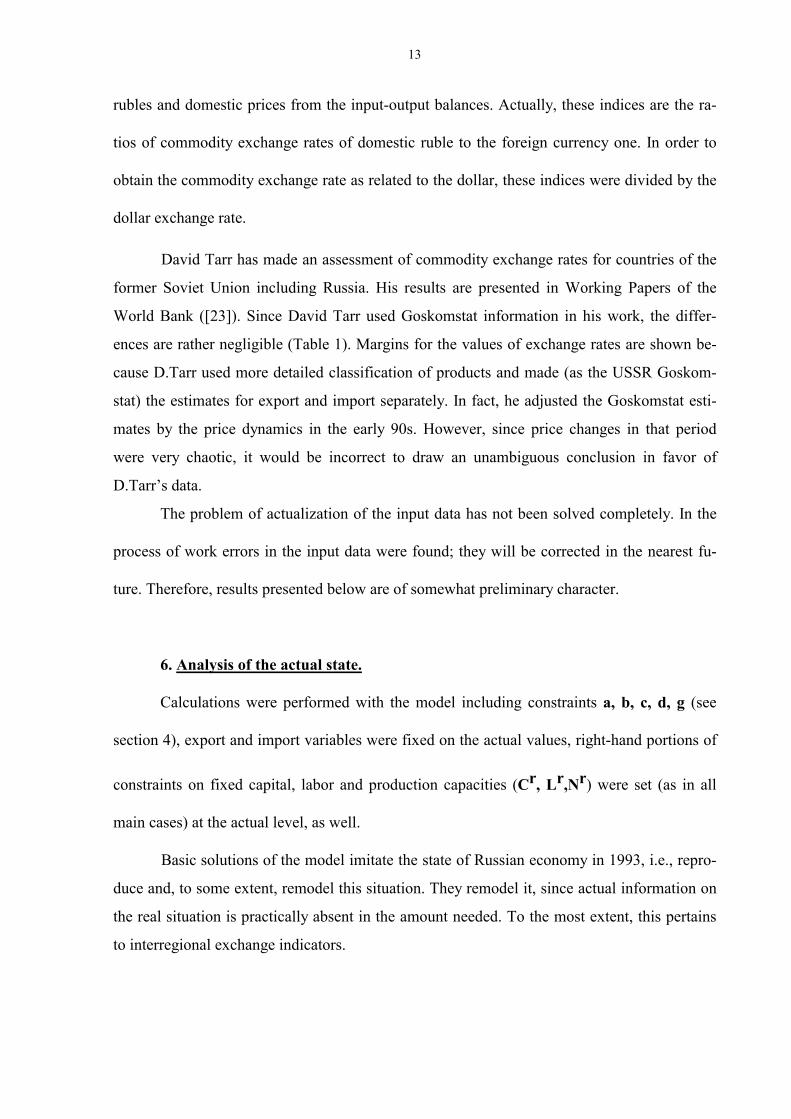
The problem of actualization of the input data has not been solved completely. In the

process of work errors in the input data were found; they will be corrected in the nearest fu-

ture. Therefore, results presented below are of somewhat preliminary character.

6. Analysis of the actual state.

Calculations were performed with the model including constraints a, b, c, d, g (see

section 4), export and import variables were fixed on the actual values, right-hand portions of

constraints on fixed capital, labor and production capacities (Cr, Lr,Nr) were set (as in all

main cases) at the actual level, as well.

Basic solutions of the model imitate the state of Russian economy in 1993, i.e., repro-

duce and, to some extent, remodel this situation. They remodel it, since actual information on

the real situation is practically absent in the amount needed. To the most extent, this pertains

to interregional exchange indicators.

14

Table 1Various estimates of foreign-to-domestic price ratio

Industries David Tarr’s estimates(World Bank)

Goskomstat estimates

1.Power industry 1,500 1,4902. Oil industry 3,540 3,3103. Oil-processing industry 2,000 1,0704. Gas industry 2,460 2,1405. Ferrous ores 0,902 1,0006. Ferrous metals 0,70-1,50 1,1807. Non-ferrous ores 1,20-1,50 0,7008. Non-ferrous metals 1,50-1,60 1,5709. Basic chemistry 0,70-1,20 0,74010. Petrochemistry 0,60-0,90 0,60311. Machine building 0,90-1,40 1,20012. Timber industry 0,700 0,79013. Woodworking industry 0,75-0,80 0,72014. Pulp and paper industry 0,78-0,81 0,76015. Textile industry 0,25-0,33 0,39016. Clothing industry 0,327 0,33017. Meat and dairy industry 0,30-0,50 0,38018. Fish industry 0,451 0,48019. Other food processing in-dustry

0,431 0,390

20. Flour-grinding and cerealsindustry

0,434

0,640

21. Plant-growing 0,500 0,44022.Stock-raising 0,2-0,3 0,180

This exchange has plausible character for the basic solutions (Table 2): European part of Rus-

sia supplies products of engineering, consumer goods, food processing industries, agriculture;

the Urals supplies products of oil-refining, metallurgy and engineering industries; West Sibe-

ria is the main supplier of oil and gas, East Siberia - electric power and timber; Russian Far

East – sea food. The balance of interregional exchange at 1990 prices is positive for the Euro-

pean part only (Table 2, the last row – in absolute terms; Table 9, row 1 – in relative terms);

East Siberia and the Far East have particularly adverse balance.

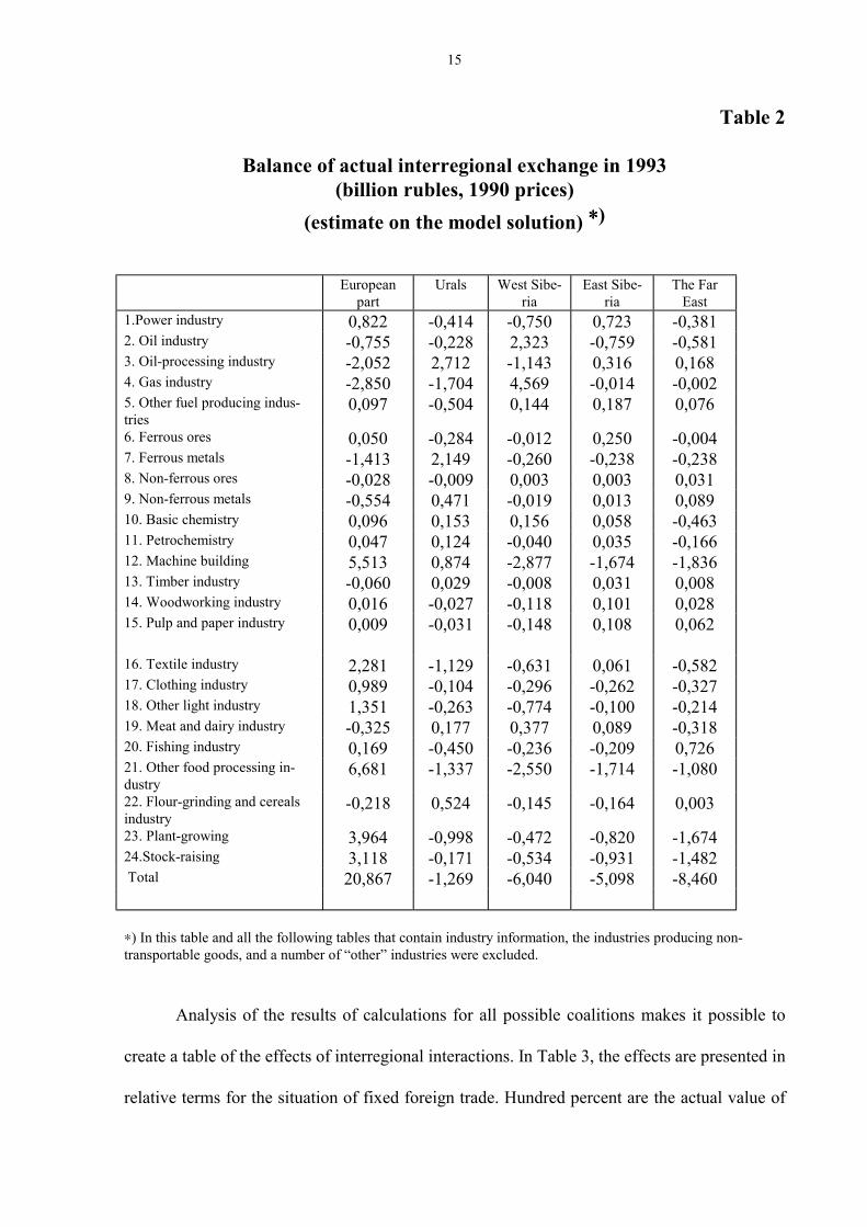
15

Table 2

Balance of actual interregional exchange in 1993(billion rubles, 1990 prices)

(estimate on the model solution) ∗∗∗∗)

Europeanpart

Urals West Sibe-ria

East Sibe-ria

The FarEast

1.Power industry 0,822 -0,414 -0,750 0,723 -0,3812. Oil industry -0,755 -0,228 2,323 -0,759 -0,5813. Oil-processing industry -2,052 2,712 -1,143 0,316 0,1684. Gas industry -2,850 -1,704 4,569 -0,014 -0,0025. Other fuel producing indus-tries

0,097 -0,504 0,144 0,187 0,076

6. Ferrous ores 0,050 -0,284 -0,012 0,250 -0,0047. Ferrous metals -1,413 2,149 -0,260 -0,238 -0,2388. Non-ferrous ores -0,028 -0,009 0,003 0,003 0,0319. Non-ferrous metals -0,554 0,471 -0,019 0,013 0,08910. Basic chemistry 0,096 0,153 0,156 0,058 -0,46311. Petrochemistry 0,047 0,124 -0,040 0,035 -0,16612. Machine building 5,513 0,874 -2,877 -1,674 -1,83613. Timber industry -0,060 0,029 -0,008 0,031 0,00814. Woodworking industry 0,016 -0,027 -0,118 0,101 0,02815. Pulp and paper industry 0,009 -0,031 -0,148 0,108 0,062

16. Textile industry 2,281 -1,129 -0,631 0,061 -0,58217. Clothing industry 0,989 -0,104 -0,296 -0,262 -0,32718. Other light industry 1,351 -0,263 -0,774 -0,100 -0,21419. Meat and dairy industry -0,325 0,177 0,377 0,089 -0,31820. Fishing industry 0,169 -0,450 -0,236 -0,209 0,72621. Other food processing in-dustry

6,681 -1,337 -2,550 -1,714 -1,080

22. Flour-grinding and cerealsindustry

-0,218 0,524 -0,145 -0,164 0,003

23. Plant-growing 3,964 -0,998 -0,472 -0,820 -1,67424.Stock-raising 3,118 -0,171 -0,534 -0,931 -1,482 Total 20,867 -1,269 -6,040 -5,098 -8,460

∗) In this table and all the following tables that contain industry information, the industries producing non-transportable goods, and a number of “other” industries were excluded.

Analysis of the results of calculations for all possible coalitions makes it possible to

create a table of the effects of interregional interactions. In Table 3, the effects are presented in

relative terms for the situation of fixed foreign trade. Hundred percent are the actual value of

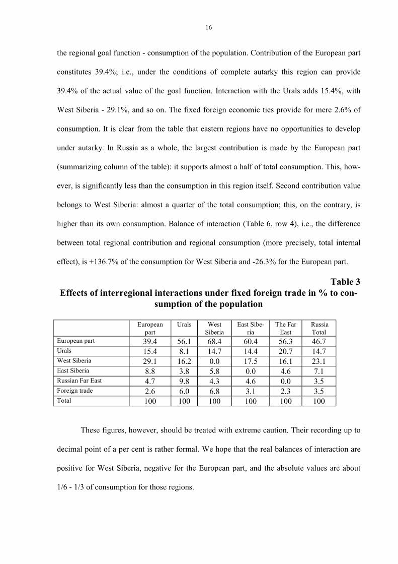
16

the regional goal function - consumption of the population. Contribution of the European part

constitutes 39.4%; i.e., under the conditions of complete autarky this region can provide

39.4% of the actual value of the goal function. Interaction with the Urals adds 15.4%, with

West Siberia - 29.1%, and so on. The fixed foreign economic ties provide for mere 2.6% of

consumption. It is clear from the table that eastern regions have no opportunities to develop

under autarky. In Russia as a whole, the largest contribution is made by the European part

(summarizing column of the table): it supports almost a half of total consumption. This, how-

ever, is significantly less than the consumption in this region itself. Second contribution value

belongs to West Siberia: almost a quarter of the total consumption; this, on the contrary, is

higher than its own consumption. Balance of interaction (Table 6, row 4), i.e., the difference

between total regional contribution and regional consumption (more precisely, total internal

effect), is +136.7% of the consumption for West Siberia and -26.3% for the European part.

Table 3Effects of interregional interactions under fixed foreign trade in % to con-

sumption of the population

Europeanpart

Urals WestSiberia

East Sibe-ria

The FarEast

RussiaTotal

European part 39.4 56.1 68.4 60.4 56.3 46.7Urals 15.4 8.1 14.7 14.4 20.7 14.7West Siberia 29.1 16.2 0.0 17.5 16.1 23.1East Siberia 8.8 3.8 5.8 0.0 4.6 7.1Russian Far East 4.7 9.8 4.3 4.6 0.0 3.5Foreign trade 2.6 6.0 6.8 3.1 2.3 3.5Total 100 100 100 100 100 100

These figures, however, should be treated with extreme caution. Their recording up to

decimal point of a per cent is rather formal. We hope that the real balances of interaction are

positive for West Siberia, negative for the European part, and the absolute values are about

1/6 - 1/3 of consumption for those regions.

17

The level of non-equivalency of interregional exchange for the actual state is rather

high (Table 9, row 2). The values of balances of internal interactions in equilibrium prices

(these are dual estimates of constraints - the balances of production and distribution) are sig-

nificant and differ essentially from those in actual prices of 1990. These differences are par-

ticularly large for the European part and West Siberia. Because of the radical change in the

price structure during 1990-1993 (the structure changed in the direction of equilibrium prices),

the estimates of internal export - import balance in the actual 1993 prices apparently occupy

an intermediate position (between the first and the second row of Table 9).

Table 4Effects of interregional interactions under free foreign trade in % to con-

sumption of the population

Europeanpart

Urals West Sibe-ria

East Siberia The FarEast

RussiaTotal

European part 25,9 14,0 18,7 17,6 15,3 21,7Urals 0,9 5,3 0,5 0,5 4,7 1,2West Siberia 4,9 0,0 0,0 1,6 1,2 2,6East Siberia 3,2 -0,8 0,9 0.0 0,0 1,6The Far East 0,2 3,5 1,5 1,0 0,0 1,7Foreign ties 64,9 78,0 79,3 78,4 78,8 71,2Total 100 100 100 100 100 100

Table 5Effects of interregional interactions under regulated foreign trade in % to

consumption of the population

Europeanpart

Urals West Sibe-ria

East Siberia The FarEast

RussiaTotal

European part 27.1 32,9 37,0 34,9 32,9 31,1Urals 11,4 5,4 10,7 10,8 16,5 10,6West Siberia 20,4 15,5 0.0 19,9 17,7 14,2East Siberia 4,5 1,9 5,5 0.0 4,7 4,2The Far East 3,1 6,5 4,2 3,6 0.0 3,7Foreign ties 33,5 37,8 42,6 30,8 28,2 36,2Total 100 100 100 100 100 100

18

Table 6

Final indicators of the effects of interactions under fixed foreign trade, in% to consumption of the population ∗∗∗∗)

Europeanpart

Urals WestSiberia

East Sibe-ria

the FarEast

RussiaTotal

Own contribution 39.4 8.1 0.0 0.0 0.0 26.8Pure internal effect 58.0 85.9 93.2 96.9 97.7 69.7Total internal effect 97.4 94.0 93.2 96.9 97.7 96.5Balance of interaction -26.3 32.9 136.7 18.7 -23.7 0.0∗) The first row of the table was formed with the diagonal elements of Table 3; the third row was obtained bysubtracting the effects of foreign trade presented in row 6 in Table 3, from 100; indicators in the second row aredifferences between the corresponding indicators of the third and first rows; indicators in the fourth row wereobtained by subtracting the total internal regional effects (they are presented in relative terms in the previousrow) from the total regional contributions (they are presented in the relative terms in the total column of Table 3),and by dividing by the final regional consumption of the population.

Table 7Final indicators of the effects of interactions under free foreign trade in %

to consumption of the population

Europeanpart

Urals WestSiberia

East Sibe-ria

The FarEast

RussiaTotal

Own contribution 25,9 5,3 0.0 0.0 0.0 13,9Pure internal effect 9,2 16,7 20,7 21,6 21,2 15,9Total internal effect 35,1 22,0 20,7 21,6 21,2 29,8Balance of interaction -1,0 -10,7 10,4 9,0 3,4 0.0

Table 8Final indicators of the effects of interactions under regulated foreign trade

in % to consumption of the population

Europeanpart

Urals WestSiberia

East Sibe-ria

The FarEast

RussiaTotal

Own contribution 27,1 5,4 0.0 0.0 0.0 14,7Pure internal effect 39,4 56,8 57,4 69,2 71,8 49,1Total internal effect 66,5 62,2 57,4 69,2 71,8 63,8Balance of interaction -21,0 31,3 116,6 -5,0 -19,3 0.0

19

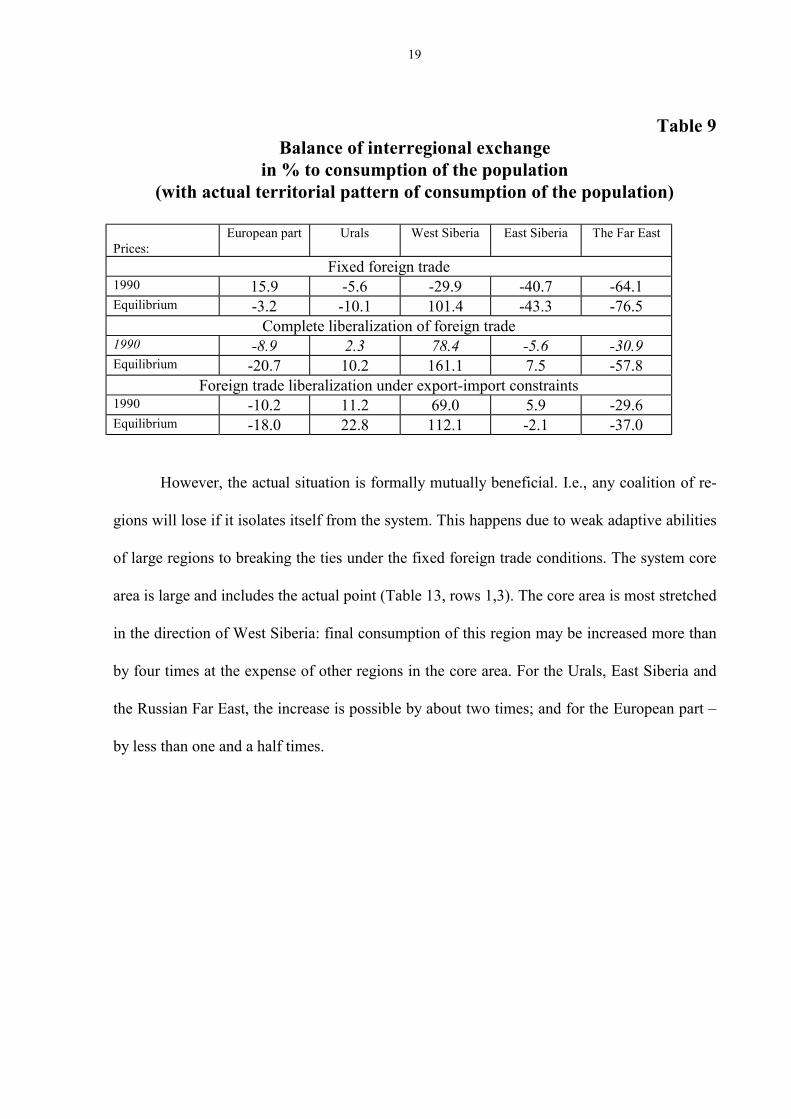
Table 9Balance of interregional exchange

in % to consumption of the population(with actual territorial pattern of consumption of the population)

Prices:European part Urals West Siberia East Siberia The Far East

Fixed foreign trade1990 15.9 -5.6 -29.9 -40.7 -64.1Equilibrium -3.2 -10.1 101.4 -43.3 -76.5

Complete liberalization of foreign trade1990 -8.9 2.3 78.4 -5.6 -30.9Equilibrium -20.7 10.2 161.1 7.5 -57.8

Foreign trade liberalization under export-import constraints1990 -10.2 11.2 69.0 5.9 -29.6Equilibrium -18.0 22.8 112.1 -2.1 -37.0

However, the actual situation is formally mutually beneficial. I.e., any coalition of re-

gions will lose if it isolates itself from the system. This happens due to weak adaptive abilities

of large regions to breaking the ties under the fixed foreign trade conditions. The system core

area is large and includes the actual point (Table 13, rows 1,3). The core area is most stretched

in the direction of West Siberia: final consumption of this region may be increased more than

by four times at the expense of other regions in the core area. For the Urals, East Siberia and

the Russian Far East, the increase is possible by about two times; and for the European part –

by less than one and a half times.

20

Table 10

Balance of export-import(billion rubles, 1990 prices)

Actual Completely free foreigntrade

Regulated foreign trade

Domesticprices

Worldprices

Domesticprices

Worldprices

Domesticprices

Worldprices

1.Power industry 0,373 0,556 -1,878 -2,798 -2,446 -3,6442. Oil industry 5,583 18,480 12,445 41,193 8,688 28,7573. Oil-processing industry 4,282 4,582 -14,612 -15,635 -3,480 -3,7244. Gas industry 3,136 6,711 1,952 4,177 1,915 4,0985. Other fuel producing indus-tries

0,589 0,477 0,023 0,019 0,000 0,000

6. Ferrous ores 0,373 0,373 0,367 0,367 0,367 0,3677. Ferrous metals 4,755 5,611 4,494 5,303 4,465 5,2698. Non-ferrous ores -0,021 -0,015 -0,034 -0,024 -0,033 -0,0239. Non-ferrous metals 5,962 9,360 5,649 8,869 5,669 8,90010. Basic chemistry 1,342 0,993 -1,473 -1,090 -1,255 -0,92911. Petrochemistry 2,572 1,620 1,791 1,128 1,803 1,13612. Machine building 2,797 3,356 -5,387 -6,464 -5,609 -6,73113. Timber industry 1,181 0,933 1,225 0,968 1,132 0,89414. Woodworking industry 1,763 1,269 -0,259 -0,186 -0,235 -0,16915. Pulp and paper industry 1,020 0,775 0,761 0,578 0,729 0,554

16. Textile industry -3,218 -1,255 -11,084 -4,323 -10,345 -4,03417. Clothing industry -2,953 -0,974 -9,730 -3,211 -9,053 -2,98718. Other light industry -2,748 -1,071 -6,949 -2,710 -6,533 -2,54719. Meat and dairy industry -4,870 -1,851 -30,590 -11,624 -17,984 -6,83420. Fish industry 0,185 0,089 -1,235 -0,593 -1,193 -0,57321. Other food processing in-dustry

-7,031 -2,742 -31,636 -12,338 -30,474 -11,885

22. Flour-grinding and cerealsindustry

0,174 0,111 3,149 2,015 -0,009 -0,006

23. Plant-growing -5,620 -2,473 5,447 2,397 -7,247 -3,18924.Stock-raising -0,163 -0,029 -27,434 -4,938 -9,556 -1,720Total 11,893 46,899 -107,840 0,001 -83,286 0,008

21

Table 11Equilibrium prices under completely free foreign trade

Europeanpart

Urals West Sibe-ria

East Sibe-ria

The FarEast

Commod-ity ex-

change rateof the ruble

1.Power industry 2,571 2,556 2,545 2,519 2,492 1,4902. Oil industry 5,710 5,660 5,632 5,631 5,535 3,3103. Oil-processing industry 1,852 1,837 1,829 1,822 1,840 1,0704. Gas industry 3,708 3,679 3,633 3,655 3,566 2,1405. Other fuel producing indus-tries

1,393 1,395 1,391 1,358 1,345 0,810

6. Ferrous ores 1,724 1,717 1,700 1,688 1,684 1,0007. Ferrous metals 2,037 2,020 2,013 2,003 1,981 1,1808. Non-ferrous ores 1,211 1,201 1,196 1,191 1,171 0,7009. Non-ferrous metals 2,713 2,688 2,678 2,661 2,632 1,57010. Basic chemistry 1,280 1,269 1,264 1,251 1,245 0,74011.Petrochemistry 1,087 1,078 1,076 1,065 1,059 0,60312. Machine building 2,072 2,054 2,048 2,037 2,015 1,20013. Timber industry 1,358 1,346 1,338 1,324 1,312 0,79014. Woodworking industry 1,241 1,236 1,232 1,215 1,202 0,72015. Pulp and paper industry 1,310 1,306 1,301 1,281 2,268 0,76016. Textile industry 0,674 0,669 0,666 0,663 0,655 0,390

17. Clothing industry 0,570 0,566 0,563 0,560 0,554 0,33018. Other light industry 0,674 0,668 0,665 0,662 0,655 0,39019. Meat and dairy industry 0,660 0,655 0,653 0,652 0,644 0,38020. Fish industry 0,832 0,826 0,823 0,821 0,798 0,48021. Other food processing in-dustry

0,675 0,670 0,667 0,664 0,657 0,390

22. Flour-grinding and cerealsindustry

1,104 1,094 1,094 1,090 1,069 0,640

23. Plant-growing 0,752 0,744 0,763 0,765 0,755 0,44024.Stock-raising 0,316 0,314 0,314 0,317 0,312 0,180Exchange rate of dollar (dualprices of e)

1,727 1,713 1,705 1,696 1,677

22

Table 12Equilibrium prices under regulated foreign trade and export-import tariffs

Euro-peanpart

Urals WestSiberia

EastSiberia

TheFarEast

Tariffs Share oftariff ininternal

price

Com-modity

ex-changerate of

theruble

1.Power industry 2,052 2,097 2,072 2,032 2,096 0,023 (i) 1,1 1,4902. Oil industry 3,579 3,561 3,501 3,599 3,731 1,08 (e) 28,9-30,8 3,3103. Oil-processing indus-try

1,639 1,586 1,616 1,576 1,511 0,127 (i) 7,7-8,4 1,070

4. Gas industry 3,027 3,018 2,954 3,022 3,057 2,1405. Other fuel producingindustries

1,136 1,203 1,191 1,118 1,135 0,810

6. Ferrous ores 1,407 1,408 1,383 1,392 1,424 1,0007. Ferrous metals 1,663 1,657 1,668 1,683 1,705 1,1808. Non-ferrous ores 0,988 0,985 0,973 0,983 0,989 0,7009. Non-ferrous metals 2,227 2,205 2,194 2,195 2,225 1,57010. Basic chemistry 1,045 1,041 1,029 1,032 1,052 0,74011. Petrochemistry 0,887 0,884 0,889 0,918 0,947 0,017 (e) 1,8-1,9 0,60312. Machine building 1,691 1,707 1,718 1,733 1,755 0,051 (i) 2,9-3,0 1,20013. Timber industry 1,120 1,103 1,088 1,090 1,107 0,79014. Woodworking in-dustry

1,013 1,053 1,082 1,049 1,016 0,079 (i) 7,3-7,8 0,720

15. Pulp and paper in-dustry

1,069 1,108 1,096 1,056 1,071 0.037 (e) 3,3-3,5 0,760

16. Textile industry 0,550 0,547 0,542 0,547 0,554 0,39017. Clothing industry 0,466 0,461 0,458 0,463 0,469 0,33018. Other light industry 0,550 0,554 0,541 0,546 0,554 0,39019. Meat and dairy in-dustry

1,162 1,161 1,156 1,163 1,169 0,626 (i) 53,6-54,2 0,380

20. Fishing industry 0,680 0,678 0,671 0,679 0,614 0,48021. Other food process-ing industry

0,551 0,549 0,543 0,549 0,556 0,390

22. Flour-grinding andcereals industry

0,901 0,868 0,891 0,900 0,875 0,02 (i) 2,2-2,3 0,640

23. Plant-growing 0,628 0,543 0,622 0,635 0,640 0,44024.Stock-raising 0,352 0,370 0,359 0,375 0,377 0,127 (i) 33,7-36,1 0,180Dollar exchange rate(Dual prices of e)

1,409 1,395 1,399 1,386 1,417

23

Table 13Regional pattern of consumption of the population

(parameters λλλλr)European

partUrals West Siberia East Siberia the Far East

under the exogenous foreign tradeActual 65.4 11.6 10.1 6.3 6.6Equilibrium 65.8 10.5 18.7 3.5 1.5Core boundaries 32-90 1-28 0-44 0-16 0-16

complete foreign trade liberalizationEquilibrium 52.1 12.7 26.5 5.8 2.9At world prices 50.5 14.5 26.7 5.5 2.8Core boundaries 2.1 2.7 6.5 .8 .9

Foreign trade liberalization under the export-import restrictionsEquilibrium 52.0 12.6 26.8 5.7 2.9At world pricesв 50.2 14.1 27.2 5.6 2.9Core boundaries 21-78 3-15 6-30 0-8 0-7

7. Foreign trade liberalization.

Consequences of the foreign trade liberalization are estimated. The variables of export

and import (vr, wr) become endogenous and c constraints (see Section 4) on the regional bal-

ance of foreign trade are imposed. In the calculations these balances were assumed to be equal

to zero (Sr = 0). The decisive role in such model experiments belongs to the commodity ex-

change rates of the ruble (parameters pr). Their values are presented in the last columns of

Tables 11 and 12. As is seen, domestic prices differ essentially from the world ones: oil price

is more than by 3 times lower than the world price; price of stock-raising products – by more

than 5 times higher than world one. This predetermines very serious consequences of foreign

trade liberalization.

If territorial structure would not change and would stay on the actual level (the system

would not come to equilibrium), then the nature of interregional ties would change radically.

European part of Russia is the only region which has a positive actual balance of interregional

24

exchange, would be the importing region (Table 9, row 3); positive balance of West Siberia

would reach almost 80% of regional consumption, Urals region would get small positive bal-

ance of exchange. Measurement of these balances in equilibrium prices provides the estimates

of non-equivalence level of interregional exchange (Table 9, row 4). The level of non-

equivalence increases in comparison with the actual state under fixed foreign trade. Burden on

West Siberia grows substantially; Urals and East Siberia become recipients. European part

appears to be the biggest donor (20% of regional consumption is formed at the expense of

other regions).

Further on, the system is brought to equilibrium (equivalent exchange). Foreign trade

turnover increases significantly (as compared with the actual turnover), foreign trade pattern

changes (Table 10, columns 3,4 в in comparison with columns 1,2). Oil export increases more

than by 3 times, import of light, food and stock-raising industry products increases by 3, 4 and

more times. Russia becomes an importer of oil-processing and engineering products; sign of

export-import balance changes for several other products too.

Domestic equilibrium prices for the above situation are presented in Table 11. They

coincide with the world market prices with an accuracy of transportation costs. Data from the

Table gives proof to this: if domestic price is divided by exchange rate of the dollar (in rubles)

given in the last row of the table (these are dual estimates of constraints on the regional bal-

ances of foreign trade), then the result will be similar (with an accuracy of transportation

costs) to the commodity exchange rate of ruble.

Complete foreign trade liberalization results in:

a) consumption increased by 1.5; consumption in West Siberia increased more than by

4 times;

b) on the average, employment decreased almost by 10 percent points (it was particu-

larly significant in the Russian Far East, East Siberia and in the Urals)

25

c) total destruction of stock-raising, oil-refining, meat and dairy industries, cata-

strophic decrease of production in consumer goods and food processing industries;

d) practically complete disintegration of the internal economic space: the regions do

not exchange products, they operate in the world market only.

Export proceeds from oil, gas, metals, timber are used for the import of oil-refining

products, consumer goods, food products and some other products. As for the regional con-

sumption pattern, West Siberia’s share had risen, share of the European part had decreased

essentially (Table 13, rows 4,5). The system core is reduced to a single point - the state of

equilibrium (in Table 13, row 6, the core is presented as a point that coincides with the equi-

librium).

It is like the situation in the recent past, but in exaggerated and even caricatured form.

Interaction effects were estimated in order to compare with the previous version. They

are presented in Tables 4 and 7. Effects of foreign trade are the most important: they amount

to almost 80% of regional consumption. With the complete economic disintegration of inter-

nal space these effects should be equal to 100%. But, as the weak ties among regions, par-

ticularly in some coalitions, still do exist, the effects of interregional interactions have rather

low values. They are not of any particular interest.

8. State control of the foreign trade.

Therefore, complete foreign trade liberalization is damaging the Russian economy.

Protectionist measures are necessary. In the analysis in question, they were introduced in two

ways. First, export tariffs were introduced on primary fuel, metals, lumber products. As a re-

sult, domestic prices of these products decreased and they became affordable for Russian con-

sumers. Second, import tariffs were introduced on the products of some processing industries.

As a consequence, domestic prices of such products grew and they became profitable. The

26

consequences of the unified customs policy for the country were tested, i.e., the system of

macro-regions was regarded as the customs union (as compared with previous variant, i con-

straints were introduced in the model, their dual values are interpreted as export-import tar-

iffs). The value of export and import duties was fixed in such a manner so as to allow to keep

all industries at the level not lower than 90% of the production in 1993.

In the model solutions under actual territorial pattern of consumption of the popula-

tion, interregional turnover at actual 1990 prices does not decrease as compared with the

situation of totally free foreign trade (Table 9, rows 5,6). A new quality is that East Siberia

becomes a region with positive balance of internal exchange. However, the level of non-

equivalence of exchange (balance at equilibrium prices) decreases. On the contrary, East Sibe-

ria, instead of being a recipient, becomes a donor.

Then, as before, the system was transformed into equilibrium state (equivalent ex-

change). In comparison with the previous case, export-import volumes are reduced, mainly

due to oil export and import of meat, dairy and stock-raising products (Table 10, columns

5,6). Signs of export-import balances change in two industries only. Exchange rate of dollar

falls dramatically, i.e., the ruble gets stronger (compare the last rows of Tables 11, 12). Do-

mestic equilibrium prices, as it was conceived, begin to differ from world prices (Table 12).

For instance, if we add export tariff to domestic oil price (column 6) and divide the result by

dollar exchange rate, the world price will be obtained (the corresponding commodity ex-

change value of the ruble). Foreign trade tariffs are essential for three industries only (Table

12, column 7): oil industry (export tariff is almost 30% of domestic price), meat and dairy

industry (import tariff is more than half of domestic price), and stock-raising (import tariff is a

little higher than 1/3 of domestic price).

As the result of foreign trade regulation, consumption in the country decreased on the

average by 5%, employment increased (it reached the level of 1993 - 88% of active popula-

27

tion); internal commodity exchange has been restored, but not in full measure. Equilibrium

regional structure of the final consumption almost did not change, as compared to the case of

complete foreign trade liberalization (Table 13, rows 4,7,8). The system core expanded (Ta-

ble 13, row 9), but remained remarkably narrower than in the case of fixed foreign trade.

In Tables 5, 8 (effects of interactions), the effect of foreign trade decreased by 2 times

(in comparison with the case of completely free foreign trade), the effects of interregional ex-

change became more substantial.

Table 14Differentiation of per capita consumption

(in % to the Russian mean)

Europeanpart

Ural West Sibe-ria

East Sibe-ria

The FarEast

Fact of 1993:In model 101 84 99 102 129RF GoskomstatData

103 88 87 90 129

Equilibrium,Foreign trade:Fixed 102 76 183 57 29Free 81 92 260 94 57Regulated 80 91 263 92 57

The shares of East Siberia and the Far East are understated in the equilibrium (i.e.,

equivalent exchange) regional structure of consumption, particularly under the conditions of

exogenous foreign trade (Table 13, row 2), (to a certain extent it may be due to the fact that

some factors were not taken into account). Per capita income in these regions decreases by

1.5-2 times under equivalent exchange. High regional disparities in per capita consumption

(Table 14) can cause the disintegration of the country. Interregional exchange within a federal

state does not have to be equivalent in order that internal economic space is sufficiently ho-

mogeneous; and interregional differences in living standards are not very large. Certain redis-

tribution of financial and other resources is required. However, the level of exchange non-

28

equivalence and volumes of transfers (and other gratuitous transfers of financial resources –

subsidies, budget financing) must be reasonable. The values of the interregional redistribution

of financial resources supporting the non-equivalence of the interregional exchange, for the

actual level of 1993, are the balances of interregional exchange in equilibrium prices pre-

sented in Table 9. For fixed foreign trade, they amount to about 10% of the total consumption

of the population or about 7% of the GDP. Under completely free foreign trade, noticeably

higher volume of financial redistribution – about 17% of total consumption or almost 12% of

the GDP (row 4)- is required in order to support the actual level of non-equivalence of ex-

change. The need in financial redistribution goes to 13% of total consumption or 9% of GDP

(row 6) due to regulation of foreign trade. Apparently, it is not that much, because currently

(1996-1997) about 5% of GDP is redistributed via the budget channels. The point is whether

the level of exchange non-equivalence is sufficient; it evidently requires further investigations.

Table 15Indices of volumes of production in % to 1990

Europeanpart

Urals WestSiberia

EastSiberia

The FarEast

Russia

1996 (estimate) 41 49 60 56 41 46Solution of the model

Complete foreign trade liber-alization

48 50 59 56 46 50

Regulation of the foreigntrade

57 55 65 62 51 58

Expert estimation of an influence of foreign trade regime changing64 64 71 69 61 67

Expert estimation of chare of other factors39 31 28 30 34 37

In this study, the impact of changes in foreign trade regime on the Russian economy

and its macro-regions, was explored. In particular, it was shown that foreign trade liberaliza-

tion results in the decrease in internal production. It is possible to estimate significance of the

29

influence of this factor on the total decrease of production in Russia. Table 15 proves that the

actual drop in production from 1990 to 1996 in Russia was 54% . The model solutions show

that complete liberalization of foreign trade would result in decrease of production by 50%

and under state control – by 42%. Such decline, only as the result of one factor impact, would

take place if market mechanisms have turned the system into equilibrium.

If we assume that only ¾ of this task was actually completed, and the two hypothetical

situations considered (complete liberalization and state regulation of foreign trade) are imple-

mented in practice with equal weights (0.5 and 0.5), then the actual decrease related with the

change in foreign trade regime amounts to merely 33% (row 4). I.e., other factors (reduction

of investment, financial disproportion, etc.) determine 21 percentage points of production de-

cline. Their share equals to 37% (additional row of the table). The most significant influence

of other factors takes place in the European part (39%). On the contrary, the consequences of

foreign trade liberalization reduced production in West and East Siberia, and in the Urals to

the highest extent.

9. General context of the study.

The above results are assumed to be the most essential for the first stage of the project.

They were obtained for the three situations; each of them includes free (optimized) internal

(interregional) trade, i.e., the country is regarded as a free trade area:

A) exogenous (fixed on the actual level) foreign trade - section 6;

B) endogenous (optimized ) foreign trade (regional balances of the foreign trade are

fixed at zero level) – section 7;

C) export-import constraints common for the entire country (the country as a common

customs area), providing for the level of production not less than 90% of the actual values in

1993 – section 8.

30

The equilibrium and the core were determined for each of the situations, the effects of

interregional (internal and foreign) interactions were estimated.

Pre-project studies and the work at the first stage of the project were carried out on a

wider scale. 7 possible situations were considered:

a) exogenous (fixed on the actual level) internal and foreign trade, i.e., the economy is

entirely centralized (usual regional input-output models are employed: a, b, c, d, g constraints

and fixed variables of internal and external links xrs, xsr, vr, wr);

b) internal trade becomes free (this condition stands in all further situations), i.e., the

situation is equivalent to the A);

c) production capacity expansion is allowed (above and beyond the actual values in

1993), i.e., the inter-industry redistribution of fixed capital within the limits of its actual value

in the region is permitted (for all industries except mining in several regions the capacities are

increased by 10% of Nr);

d) technological substitution of some products is permitted; e.g., coal for natu-

ral gas in power industry (two-component modes of substitution are introduced in

the model: in balance of output a which is substituted, the mode has component

«+1»; in the balance of output which substitutes, the norm of substitution has a

negative sign;

e) foreign trade becomes endogenous under the actual value of regional balances of

foreign trade in 1993; in comparison with situation (B) Sr is fixed at the actual level, but not

at the zero one;

f) in comparison with case (e), f constraints (see section 4) on the regional export un-

der the actual level in 1993 are imposed;

31

g) in comparison with case (e), f constraints on the regional import wr at the actual

level of 1993 are imposed.

The effects of interregional exchange were estimated for all these situations and core

boundaries were found for all of them, except for situations a) and e). For situation a) it is

impossible to find the core, because the regional pattern of consumption (final demand of the

population) can not change; in situation e) the calculations remained unfinished and equilib-

rium points were not found.

The results are presented in the Tables 16-19 (these tables were adduced with the small

differences in the preceding report). The rows of the table are 7 situations. Five columns of the

table are total columns in the table of effects of interregional interactions. The second row of

this table coincides with the total column of Table 3 (as situations A) and b) are equivalent).

The second rows of Tables 17, 18, 19 coincide with the total column of Table 6, with the

fourth row of Table 6, and with the third row of Table 13, respectively.

Table 16Contributions of the regions to the consumption of population (%)

Europeanpart

Urals WestSiberia

East Sibe-ria

the FarEast

Foreignties

Actual state 32.5 12.3 11.9 11.9 11.9 19.5Endogenous internaltrade

46.7 14.7 23.1 7.1 4.9 3.5

Capacity expansion 47.1 12.0 24.2 3.9 6.0 6.8Substitution of products 50.6 22.0 9.8 6.1 6.1 5.4Endogenous foreigntrade

31.5 2.2 8.2 0.6 -0.9 58.4

Constraints on export 41.5 6.0 6.3 1.9 0.5 43.8Constraints on import 45.2 3.2 23.4 4.5 4.7 19.0

The information contained in these tables is too large to be analyzed in the framework

of the project. That is why the results presented above relate only to a small portion of this

information. Nevertheless, some general remarks may be made.

32

The role of West Siberia is decreased noticeably when substitution of some products is

allowed; particularly, gas and coal in the power industry (Table 16), as Russian regions in this

case become less sensitive to the break of ties with West Siberia.

Table 17Indices of the effects of interactions in % to population’s consumption

Own contribution Pure internal effect Total internal effectActual situation 26.8 53.7 80.5Endogenous internaltrade

26.8 69.7 96.5

Capacity expansion 27.0 66.2 93.2Substitution of products 28.3 66.3 94.6Endogenous foreigntrade

23.8 17.8 41.8

Constraints on export 25.8 30.4 69.6Constraints on import 26.4 54.6 81.0

The liberalization of the foreign trade results in sharp increase of the foreign trade ef-

fect. The contribution of the foreign trade constitutes more than a half of the final consump-

tion of the country (Table 16).

In the centralized economy the role of East Siberia and the Far East were significant,

the contribution of these regions into the Russian consumption was higher than their own con-

sumption. After liberalization of internal trade the, situation changes to the opposite: their

balances of interaction become negative (Table 19).

33

Table 18Balance of interactions of the regions in % to population’s consumption

Europeanpart

Urals West Siberia East Siberia the Far East

Actual state -31.4 25.6 33.3 118.9 104.7Endogenous internal trade -26.3 32.9 136.7 18.7 -23.7Capacity expansion -22.0 13.0 150.4 -32.7 -5.0Substitution of products -16.5 91.3 3.7 2.2 -4.2Endogenous foreign trade 0.8 -12.3 69.8 -32.6 -63.2Constraints on export 0.5 57.2 -3.4 -39.2 -64.1Constraints on import -11.6 -53.4 153.3 -12.8 -14.3

10. Political implications of the project

In our opinion, integral estimates of the Russian economic space quality under the

conditions of the free market relations obtained in this study, (the level of interregional ex-

change non-equivalence, value of the payments actually received from the resource-extracting

regions, the level of territorial differentiation by the living standards of the population), the

roles of particular regions in supporting the Russian statehood, the trends of changes in the

above indicators, are important “food for thought” for politicians. The obtained values of ex-

port-import tariffs, volumes of interregional redistribution of financial resources, can find

practical implication. The ideology of the project, which considers Russian regions as a free

market system that is regulated with the “civilized” tools by the state, may have certain politi-

cal repercussions.

34

Table 19The possible change in the regional structure of population’s consumption

(parameters λλλλr) within the limits of the system core

Europeanpart

Urals West Siberia East Siberia the Far East

Actual state is not calculatedEndogenous internal trade 32-90 1-28 0-44 0-16 0-16Capacity expansion 30-89 2-27 0-45 0-11 0-15Substitution of products 37-87 2-32 0-27 0-16 0-15Endogenous foreign trade Calculations were not doneConstraints on export 65-77 8-12 1-10 0-6 0-7Constraints on import 36-82 2-13 0-43 0-8 0-9

11. Conclusion

This study can be regarded as an initial stage of analysis of interactions between

macro-regions and world economy. Further, many fragments of the input data will have to be

verified, the models will be modified and the results will be tested more carefully.

References

1. Hildenbrand V. Core and equilibrium in large economy.- Moscow: Nauka, 1986.

2. Granberg A.G. Optimization of territorial proportions of national economy.- Mos-

cow: Economika, 1978.

3. Granberg A.G., Suslov V.I. Coalition analysis of multi-regional systems: theory,

methodology, results (USSR on the eve of collapse).- Novosibirsk: RAS. Siberian branch.

IEIE, 1993.

4. Granberg A.G., Suspitsin A.S. Introduction to system modeling of national econ-

omy.- Novosibirsk: Nauka. Siberian branch, 1988.

5. Optimizing interregional input-output models.- Novosibirsk: Nauka. Siberian

branch, 1989.

35

6. Suslov V.I. Estimating the effects of interregional interactions: models, methods, re-

sults.- Novosibirsk: Nauka. Siberian branch, 1991.

7. Balassa B. Trade Creation and Diversion in the European Common Market: an Ap-

praisal of the Evidence. European Economic Integration. 1975.

8. Bergstrand J. The Gravity Equation in International Trade: Some Microeconomic

Foundations and Empirical Evidence. The Review of Economics and Statistics. 1985, N 3.

9. Bergstrand J. The Generalized Gravity Equation, Monopolistic Competition and the

Factor-Proportions Theory in International Trade. The Review of Economics and Statistics.

1989, N 1.

10. Brada J., Mendez J. Economic Integration among Developed, Developing and

Centrally Planned Economies: a Comparative Analysis. The Review of Economics and Statis-

tics. 1985, N 4.

11. Caves R., Frankel J., Jones R. World Trade and Payments, 1992.

12. Kreinin M. Effects of the EEC on Imports of Manufactures. Economic Journal.

1972, vol. 82.

13. Krugman P., Obstfeld M. International Economics: Theory and Policy.

14. Krugman P. Intra-industry Specialization and the Gain from Trade. Journal of Po-

litical Economy, 1981.

15. Robson P. The Economics of International Integration. 1987.

16. Tinbergen J. Shaping the World Economy: Suggestions for an International Eco-

nomic Policy. 1962.

17. Truman E. The Effects of European Economic Integration on the Production and

Trade of Manufactured Products. European Economic Integration. 1975.

18. Vickerman R. The Single European Market: Prospects for Economic Integration.

1992.

36

19. Sodestren D., Reed G. International Economics.1994

20. Alesina A., Rodrik D. Distributive politics and Economic Growth. Quarterly Jour-

nal of Economics, v. CIX, 1994.

21. Competition among States and Local Governments: Efficiency and Equity in

American Federalism. 1991.

22. Eaton B., White W. The Distribution of Wealth and the Efficiency of Institutions.

Economic Inquiry, XXIX, 1991.

23. Tarr D.G. How Moving to World Prices Affect the Terms of Trade in 15 Countries

of the Former Soviet Union. Country Economics Department. The World Bank, 1993, WPS

1074.