1

Developing a New Classification of Urban and Rural Areas for Policy Purposes – the Methodology

Peter Bibby, School of Town and Regional Planning, University of Sheffield

and

John Shepherd,

School of Geography, Birkbeck College, Director, Defra Rural Evidence Research Centre

1. Introduction 1.1 In 2001 the Office of the Deputy Prime Minister (ODPM) – then the

Department of Transport Local Government and the Regions (DTLR) – commissioned a wide-ranging review of the definitions of urban and rural areas in use for policy purposes and statistical reporting. The review covered both England and Wales and involved consultations with over twenty-five Government Departments and sections within them.1

1.2 The need for such a study had been recognised for some time and was

reinforced during data gathering and analysis for the Urban and Rural White Papers.2 The review had five main objectives including the need to identify those policies that required definitions of urban and rural areas and to suggest a ‘core’ set of definitions that met a wide range of policy needs. Importantly, the review was also to ‘… identify any new techniques that could better meet established and anticipated needs.’3

1.3 The review recommended that the ‘core’ definitions of ‘urban’ and

‘rural’ should, in the medium term, comprise the DTLR (now ODPM), 1991 ‘urban area’ boundaries with their census-based populations4 and the Countryside Agency’s administrative area classification of urban and rural local authority districts and wards. However, in the rural domain, both the urban areas and the administrative area definitions

1 A Review of Urban and Rural Definitions, Project Report, 2001, http://www.statistics.gov.uk/geography/downloads/Project%20Report_22%20AugONS.pdf. 2 Our Towns and Cities: the Future, Delivering an Urban Renaissance Cm 4911 TSO 2000, Our Countryside: the Future. A Fair Deal for Rural England, Cm 4909, TSO 2000 3 op cit para 1.1.2 4 Now updated to 2001

2

had a number of drawbacks, especially in relation to evolving rural policy on service delivery. The review recommended that a clearer, more comprehensive approach to rural area definition was needed. In essence this would involve the extension of the ‘land use’ approach that underlay the urban areas definition in order to identify, define and derive populations for the small towns, villages, hamlets and isolated dwellings that made up the settlement pattern of rural areas.

1.4 In early 2002 five Government bodies, namely the Department for

Environment, Food and Rural Affairs (Defra), the Office of the Deputy Prime Minister (ODPM), the Office for National Statistics, the Welsh Assembly Government and the Countryside Agency, formed a consortium to commission a new definition of urban and rural areas using the approach recommended in the review report.

1.5 The group charged with implementing and validating the new definition

comprised the South East Regional Research Laboratory (SERRL), at Birkbeck College, the School of Town and Regional Planning at Sheffield University, the School of Computing at the University of Glamorgan and Geowise Ltd of Edinburgh. This note describes the methodologies used and the key decisions taken in developing a new definition and classification of smaller urban areas and rural settlements in England and Wales.

2. Abstract: The New Definition of Rural Places 2.1 The remit for producing a new rural/urban definition stated that this

should apply to those places which lay outside Census Urban Areas with a population of 10,000 or more.5 The methodology for defining rural places described here is thus applied to settlements otherwise described as ‘Urban Areas’ with between 10,000 and roughly 1,500 population. However, the definition of ‘rurality’ with which we are concerned reaches much further down the settlement hierarchy to small villages, hamlets and isolated dwellings.

2.2 The identification of rural settlements is derived from a grid covering

England and Wales with some 35 million cells each of 1ha. Individual residential addresses are captured where they occur within this grid forming a pattern of household densities that is used as a proxy for residential land use at a high degree of resolution. Residential densities are then averaged for each cell using a set of varying radii around each cell. The result is the creation of a ‘density profile’ typifying settlements and enabling, via a set of rules, a classification of settlement types.

2.3 The next stage is to relate rural settlements to Census Output Areas and to classify them by settlement type. This classification is based upon the proportion of the population within each Output Area in

5 See Census 2001 Key Statistics for Urban Areas, Office for National Statistics 2001

3

settlements of various kinds. Using the same general approach, residential densities are also averaged at a series of much larger geographic scales to give a ‘context’ measure for settlements reflecting the wider ‘sparsity’ of the population. The classifications of Output Areas by settlement type and context are then brought together to create a two-level classification of rural areas as follows:

Classifications for Super Output Areas and wards by settlement type and context are built up from the composition of the classified OAs that they contain. They are also brought together to create a two-level classification of rural areas as follows:

3. Some Urban-Rural Distinctions 3.1 Although this is not the place for a discussion of whether, at the

cultural, social or economic levels, it is any longer valid to try to distinguish between the ‘urban’ and the ‘rural’,6 some comments in this area may be helpful to understanding the approach to definition and classification undertaken here.

3.2 There are at least three senses or dimensions that can be ascribed to

the word ‘urban’ and, by extension, to the word ‘rural’. One is concerned with an apparently simple distinction between land that is built over and land that is not built over. Usually, however, this

6 A discussion of matters related to this issue appears in the Review report chapters 5 and 6.

Small town and fringe Village Dispersed

Sparse

Small town and fringe Village Dispersed

Less sparse

Rural

Small town and fringe Village and Dispersed

Sparse

Small town and fringe Village and Dispersed

Less sparse

Rural

4

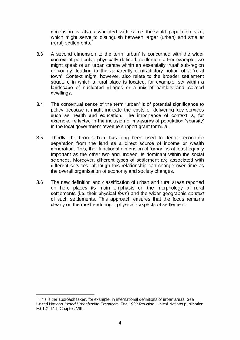
dimension is also associated with some threshold population size, which might serve to distinguish between larger (urban) and smaller (rural) settlements.7

3.3 A second dimension to the term ‘urban’ is concerned with the wider

context of particular, physically defined, settlements. For example, we might speak of an urban centre within an essentially ‘rural’ sub-region or county, leading to the apparently contradictory notion of a ‘rural town’. Context might, however, also relate to the broader settlement structure in which a rural place is located, for example, set within a landscape of nucleated villages or a mix of hamlets and isolated dwellings.

3.4 The contextual sense of the term ‘urban’ is of potential significance to

policy because it might indicate the costs of delivering key services such as health and education. The importance of context is, for example, reflected in the inclusion of measures of population ‘sparsity’ in the local government revenue support grant formula.

3.5 Thirdly, the term ‘urban’ has long been used to denote economic

separation from the land as a direct source of income or wealth generation. This, the functional dimension of ‘urban’ is at least equally important as the other two and, indeed, is dominant within the social sciences. Moreover, different types of settlement are associated with different services, although this relationship can change over time as the overall organisation of economy and society changes.

3.6 The new definition and classification of urban and rural areas reported

on here places its main emphasis on the morphology of rural settlements (i.e. their physical form) and the wider geographic context of such settlements. This approach ensures that the focus remains clearly on the most enduring – physical - aspects of settlement.

7 This is the approach taken, for example, in international definitions of urban areas. See United Nations. World Urbanization Prospects, The 1999 Revision, United Nations publication E.01.XIII.11, Chapter. VIII.

5

4. The Basics of the Classification. 4.1 As noted above, the definition and classifications presented here build

on the recommendations of a review of urban and rural definitions as subsequently accepted by Government. The report concluded that it was appropriate for most policy purposes to employ the ‘physical settlements’ definition as represented by the ODPM defined ‘urban areas’ and to treat those with more than 10,000 people as ‘urban’.8 Given this, all other settlements are treated as part of a ‘rural’ domain.

4.2 The process of definition described here has as its initial ‘raw material’

all settlements of whatever size below 10,000.9 Identifying and locating these smaller settlements requires information at a very high level of geographic resolution. This is provided by Royal Mail’s ‘Postcode Address File’ (PAF) as packaged in its Address Manager ® product. Amongst other things, PAF contains the postal addresses of premises together with a 10m resolution OS grid reference for the unit postcode allocated to each address.

8 Note that this is irrespective of the contextual or functional characteristics of urban areas with more than 10,000 population i.e. what are regarded in the Rural White Paper as larger ‘market towns’ (op. cit. Chapter 7). 9 i.e. even though the Urban Areas definition itself relates to places with between 10,000 and c 1000 population.

6

5. Clustering Postal Addresses 5.1 The starting point in the process of creating a representation of rural

settlement – what we have called the ‘underlying settlement classification’ – is the grouping of every postal address on the basis of the 1 hectare (100m x 100m) cell within which it falls.

5.2 This process is illustrated in Figure 1, which shows, by means of the

pecked lines, some urban areas represented in the ‘core’ definition of ‘urban’. The larger central urban area (Canterbury) has more than 10,000 population and would thus not be included in the definition analyses described here. The remaining settlements are below this threshold. The variously coloured 1ha cells indicate the number of postal addresses allocated to each cell. Note the clustered and isolated coloured 1ha cells outside the pecked lines. These, along with the small urban areas, are the focus for an analytical process designed, in the first instance, to classify rural settlement on the basis of settlement type or ‘morphology’.

Figure 1: Household Densities in 1ha Cells

7

6. Constructing the Underlying Settlement Classification. 6.1 As noted above, the allocation of residential addresses to a regular grid

immediately allows examination of the density of households at the 1ha cell level. Using the 2001 Second Quarter version of PAF means the grid is virtually coterminous with information on the distribution of households from the 2001 Census. The relationship between the two for part of England is shown Figures 2 (a) and (b).

6.2 Although the 1ha grid makes the perception and understanding of (in

this case) address densities more transparent, such densities are, in fact, partly a function of the scale at which they are measured. As areas are extended, for example, more areas of open space may be included and average densities will decline. Importantly, we can make use of this property - which gives different typical densities at different scales - in order to identify and classify rural settlements. Here we make use of the term ‘density profile’ which is used to refer to a series of density measures focused on a given 1ha cell but calculated at different scales. Furthermore, different morphologies or settlement forms can be shown to have different typical density ‘profiles’.

Figure 2a: Distribution of Households from the 2001 Census of Population

8

6.3 Consider, for example, a situation where about 50 houses stand on a

relatively small piece of land, perhaps constituting a small village. If one were to calculate density over a broader area centred on the 1ha cell containing the village (say, for 200m radius around the centre of that cell), and there were no other houses outside that cell, then the density measure calculated over this wider area would be 4 dwellings to the hectare. If one were to measure density over an area 400m around the cell, the density would fall by a factor of four, to 1 dwelling per hectare.10

6.4 The rate at which density changes away from the ‘focus’ cell is a

function of local settlement structure. Thus in a conurbation, where densities are sustained at (say) 30 dwellings to the hectare over a broader area, such falls will not occur, whereas for a village in an area of hamlets and isolated dwellings, the density ‘fall-off’ will be marked.

6.5 ‘Density profiles’ can thus be created using a series of different area or ‘window’ sizes. In other words, density profiles can be created by calculating densities at a series of fixed scales - in our case 200m, 400m, 800m and 1600m - around each cell (Figure 3). Actual

10 Clearly, at the other extreme i.e.in a city, this would not be the case, as higher densities would be maintained over larger areas.

Figure 2b: Distribution of Households from PAF 2001 Second Quarter

9

settlement patterns, of course, are not composed solely of compact villages surrounded by un-populated agricultural land. In practice, the decline of density with distance is less acute. Typically, a ‘village’ as defined here would have the following properties: a density of greater than 0.18 residences per hectare at the 800m scale, a density at least double that at the 400m scale and a density at the 200m scale at least 1.5 times the density at the 400m scale.

Figure 3: Areas for Calculating the Grid Density Gradient

Dark Green : area for calculating the 200m density Pale Green : area for calculating the 400m density Pink : area for calculating the 800m density Beige : area for calculating the 1600m density

10

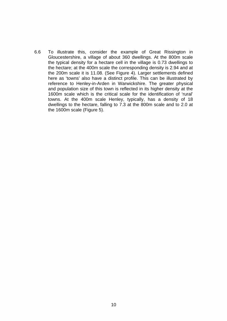
6.6 To illustrate this, consider the example of Great Rissington in Gloucestershire, a village of about 360 dwellings. At the 800m scale the typical density for a hectare cell in the village is 0.73 dwellings to the hectare; at the 400m scale the corresponding density is 2.94 and at the 200m scale it is 11.08. (See Figure 4). Larger settlements defined here as ‘towns’ also have a distinct profile. This can be illustrated by reference to Henley-in-Arden in Warwickshire. The greater physical and population size of this town is reflected in its higher density at the 1600m scale which is the critical scale for the identification of ‘rural’ towns. At the 400m scale Henley, typically, has a density of 18 dwellings to the hectare, falling to 7.3 at the 800m scale and to 2.0 at the 1600m scale (Figure 5).

11

360 dwellings

800m scale : 0.73400m scale: 2.94200m scale: 11.08.

Stow

Bourton

Northleach

Burford

Typical household densities(dwellings/ha)

Great Rissington

Figure 4 A Compact Village Identified by Density Profiles

See Figure 6 for colour codes to settlement type.

12

See Figure 6 for colour to codes settlement type.

Henley in Arden Redditch

Stratford

Alcester

Typical household densities(dwellings/ha)

c 1400 dwellings 1600m scale : 2.1 800m scale: 7.3 400m scale: 18.3

Figure 5 A Rural Town Identified By Density Profiles

13

6.7 The use of ‘density profiles’ at the sorts of geographic resolution discussed here can identify a whole range of elements within the urban and rural settlement structure. Such elements include not only a clear delineation of the boundaries of large and small urban areas where these follow residential land uses, but also such features as the ‘urban fringe’ (where there are abrupt changes of density between scales), nucleated villages and their ‘envelopes’ and areas of scattered dwellings. Areas of higher density dispersed settlement around cities and towns also have a distinct ‘peri-urban’ density profile.

6.8 In fact, the underlying settlement classification allows for the

identification of nine morphological types including, for example, ‘urban fringe’, ‘town’, ‘village’ and ‘hamlet’. Seven of these features are shown in Figure 6 – those not present in this area are hamlets and isolated farms. The numerical outcome of applying the procedure to the 1ha cells for England and Wales is shown as a set of overall average densities for each identifiable rural settlement feature in Table 1. Annex 1 provides the rules for identifying settlement morphology.

Table 1: Measured Density Profiles for Settlement Forms

Settlement Form Density of Residential Delivery Points (mean) At 200m At 400m At 800m At 1600m Small town 8.23 8.99 8.29 5.59Fringe (urban, town) 6.46 7.21 5.90 4.68Village 3.81 2.28 0.83 0.58Peri-urban 0.30 0.59 1.57 2.80Village envelope 0.94 1.15 1.31 0.59Village envelope (in peri-urban) 2.96 3.27 1.81 2.13Hamlet 0.65 0.21 0.13 0.20Scattered dwellings 0.39 0.17 0.15 0.23Urban Areas (above 10k) 16.09 15.17 13.78 11.89

Note: it is important to recognise that these data are the outcome of applying the density profile measurement procedure and hence take account of the particular environs of settlements.

6.9 Finally, use of the textual descriptions of addresses within the PAF

allows both historic and functional elements of settlements to be identified. Thus within the broad category of ‘dispersed settlements’, hamlets were identified in the developmental stages of the definition. By applying natural language processing, PAF is used to identify farmsteads and then, in the tradition of rural settlement analysis exemplified by Roberts (1996),11 to identify hamlets and larger settlement units. Clusters of 3-8 historic farmsteads within 250m of each other were identified as ‘hamlets’.

11 B K Roberts, Landscapes of Settlement, London, Routledge, 1996

14

Figure 6: A Range of Rural Settlement Features Identified by Density Profiles

urban area peri urban small town fringe (urban, town) village village envelope scattered dwellings

Moreton in Marsh

Stow on the WoldChipping Norton

Charlbury

Longborough

Evenlode

Churchill

Hook Norton

Dean

Hyde Hill

Long Compton

Ascott

15

7. Adding Context

7.1 ‘Context’, as noted above, refers to the broader setting in which settlements (including isolated dwellings) are located. In this sense context may be interpreted in general terms as the wider accessibility of a settlement, the sparsity of population within a broad area and, in a general way, the potential costs of overcoming distance to supply that settlement with various public and private services.

7.2 In just the same way as they have been used to identify settlement types, density profiles can be used at much larger scales to characterize aspects of accessibility and population sparsity. In our case this involves calculating for every 1ha cell the density of households across areas of 10,000m, 20,000m and 30,000m centred on that cell.12 Each of these context measures for a particular 1ha cell might be thought of as deriving from a household density map at the stated scale. Maps for the 10,000m and 30,000m scales are shown in Figure 7.

7.3 On the basis of these measures it is possible to identify areas where

population is ‘sparse’ at the particular scale. By assigning these measures to 2001 Census Output Areas and focusing on the sparsest 5 percent in each case, three indicators of ‘sparsity’ are obtained. The map of the grids that meet this criterion at all three scales is shown in Figure 8.

7.4 For definitional purposes (see the section headed ‘Output Areas’

below), the focus has been on areas whose population might be considered ‘sparse’ at all three scales. However, a clear distinction might be made between areas ‘sparse’ at all three scales (such as Central Wales and parts of North Devon), and those ‘sparse’ only at the 10km scale such as the Cotswolds and the White Peak of Derbyshire). This distinction has potential for further application and, as a result of comments made in the validation procedure, is being explored.

12 These scales were arrived at so as to broadly typify (at the 10,000m range) general commuting distances and, at the larger scales, the range of supply of ‘high level’ rural services such as ambulances or fire fighting vehicles. The distances selected were the result of discussion with the Project Board and empirical experimentation.

16

Figure 7: Household Densities Calculated at 10,000m and 30,000m.

(a) 10,000m (b) 30,000m

17

Figure 8 The Combined Context (Sparsity) Map

Dark Blue: ‘sparse’ at all three scales Mid Blue: ‘sparse’ at 30,000m and 20,000m Light Blue: ‘sparse’ at 10,000m

18

Considering Function 8.1 As part of the work of producing a new urban/rural definition, function

was also considered. ‘Function’ here refers to the economic character of settlements or, again and more precisely, to the 1ha cells that constitute settlements.

8.2 For this purpose, indicators were developed which distinguished cells

in accordance with the mix of residential and non-residential addresses. This allowed the definition, for example, of dormitory settlements. Moreover, using natural language processing,13 an assessment was made of the Standard Industrial Classification and town and country planning Land Use Class of each postal address on the basis of the premise described and the occupier name.

8.3 In this way, every 1ha cell was considered either to be characterized by

‘no businesses’, ‘farm businesses’, ‘tourist business’ or ‘other businesses’. These indicators were then considered alongside the morphological and context measures for possible inclusion as indicators for use in producing urban and rural definitions.

9. The Classification of Statistical and Administrative Units 9.1 Having classified individual cells, the next step is to categorise the

settlement characteristics of statistical and administrative units. This is designed to complement the use of a range of statistical data, particularly those from the decennial population census. The smallest of the units to be classified are 2001 Census Output Areas. Output Areas were introduced for the first time as a basis for publication of results of the 2001 Census.14 They are intended to represent compact, socially homogenous areas, and are designed to nest within ward and parish boundaries and hence within higher level administrative geographies.15

9.2 At a broader scale Super Output Areas and wards are also classified.

Classification depends on identifying the proportion of OAs in each urban/rural class within the area concerned.

13 P Bibby, Maps from Words, International Journal of Geographic Information Science, forthcoming 14 http://www.statistics.gov.uk/census2001/cn_40.asp 15 http://www.geog.soton.ac.uk/research/oa2001/

19

(a) Census Output Areas 9.3 At Census Output Area level, units are grouped into four morphological

types on the basis of their predominant settlement component:

• urban • small town and fringe • village, and • dispersed.

9.4 Output Areas are treated as ‘urban’ or ‘rural’ simply on the basis of their

geographic relationship to settlements of 10,000 or more population. More specifically, where the majority of the population of an Output Area lives within settlements with a population of more than 10,000 people, that Output Area is treated as urban. All other Output Areas are treated as rural. This is superimposed on the underlying settlement classification to form what is called here the ‘combined settlement classification’.

9.5 Output Areas are given a sparsity score at 10km, 20km and 30km by

producing a weighted total of 1ha squares within an Output Area, where the weights are the number of residential delivery points (rdp). Output Areas are classified as ‘sparse’ if they fall within the sparsest 5 percent of Output Areas at all three scales and are classified as ‘less sparse’ if they do not fall within this threshold. The fifth percentile ‘cut-offs’ for the application of this rule are shown in Table 2.

Table 2 Fifth Percentile Measures for Defining Sparsity

Category Fifth Percentile Sparse at the 10km scale < 0 .3932 rdp per ha Sparse at the 20km scale < 0.41 rdp per ha Sparse at the 30km scale < 0.4224 rdp per ha

9.6 It should also be noted that Output Areas are classified by ‘hierarchical

privileging’, that is, if an Output Area has 50 percent by area of a particular settlement morphology, this classification is used. However, in the very small number of cases where an Output Area did not contain a dominant morphological type then the largest settlement character is ‘privileged’ with the Output Area classification.

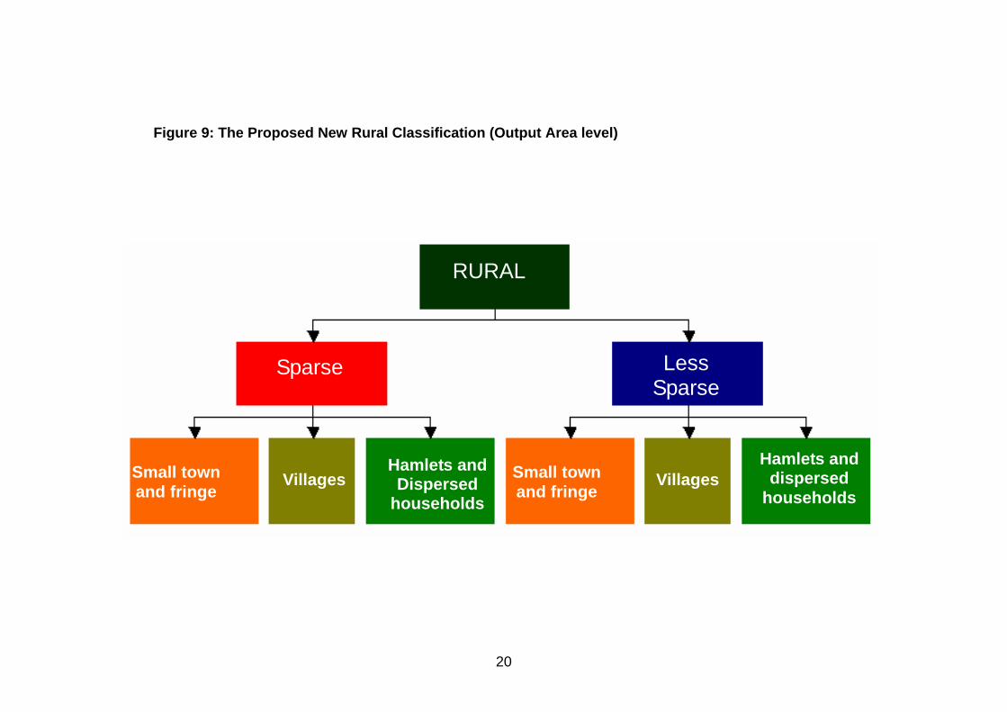
9.7 Finally, classifications on the ‘morphology’ and ‘context’ dimensions are

combined as indicated in the ‘tree diagram’ (Figure 9) and mapped in Figure 10.

20

RURAL

Sparse

Small town and fringe

VillagesHamlets andDispersed

households

Small town and fringe

Villages

Less Sparse

Hamlets anddispersed

households

Figure 9: The Proposed New Rural Classification (Output Area level)

21

Figure 10: Urban/Rural Classification of 2001 Census Output Areas

22

(b) Super Output Areas and Census Wards

9.8 The design of Super Output Areas and Wards is such that very few are

characterized by predominantly dispersed settlement (for example only 0.5 percent of wards). For this reason, only three morphological categories are distinguished:

• urban, • small town and fringe, and • village and dispersed

The methodology used to derive which of these categories each Super Output Area or Ward is allocated to has been termed the “OA count approach” and classifies the relevant geography (CAS ward, 2003 Statistical Ward, Lower Super Output Area, Middle Super Output Area) according to the predominant type of Output Area that it contains :

• A CAS Ward/2003 Statistical Ward, LSOA/MSOA is urban if the number of urban OAs it contains is greater than or equal to the number of rural OAs.

• The remaining rural CAS Ward/2003 Statistical Ward,

LSOA/MSOA are then classified as being small town/fringe if the number of small town/fringe OAs is greater than or equal to the number of village and dispersed OAs.

• The remaining unclassified CAS Ward/2003 Statistical Ward,

LSOA/MSOA are classified as village and dispersed.

9.9 Because context measures vary smoothly from 1ha cell to another, there is little difficulty in estimating measures for Super Output Areas and wards that are consistent with those measured for Output Areas, as illustrated in Figures 11a, 11b and 11c. The OA count approach is used to calculate the context measure for CAS Ward, 2003 Statistical Ward, LSOA and MSOA as follows :

• A CAS Ward/2003 Statistical Ward, LSOA/MSOA is less sparse

if the number of less sparse OAs is contains is greater than or equal to the number of sparse OAs.

• The remaining CAS Ward/2003 Statistical Ward, LSOA/MSOA

are classified as sparse.

23

Figure 11a: Urban/Rural Classification of 2001 Census Lower Super Output Areas

24

Figure 11b: Urban/Rural Classification of 2001 Census Middle Super Output Areas

25

Figure 11c: 2001 CAS Wards Classified

26

10 Local Authority Districts

10.1 Broadly speaking the same classificatory principles can be applied at larger geographic scales, depending on the settlement pattern of the area concerned. Morphological classification of local authority districts (LADs) is, however, much less straightforward. The design of territories for local authorities tends to include a mix of rural and urban areas (typically with a population of 100,000 or more). Just as the dispersed settlement category disappears when moving from the Output Area to the ward scale, a shift to the local authority district scale involves the ’collapse’ of most of the rural morphological categories.

10.2 A classification of LADs, to be useful in data analysis and policy terms,

is therefore likely to require different principles to those applied here. For this reason the project board did not recommend, at this stage, a binary (i.e. rural/urban) classification of LADs, along the same lines as the main rural definition. No doubt there will be a need to return to deeper consideration of the issue of classifying LADs, but for the moment we simply note some points for further analysis.

27

10.3 On the basis discussed above, three quarters of LADs appear as ‘urban’ in morphological terms, whilst the remainder have no predominant settlement form. This suggests that a morphological classification involving a range of urban/rural situations is required at the LAD level. While it might seem possible to distinguish those LADs that are predominantly ‘urban’ in morphological terms from others, this might appear problematic because a substantial number of LADs are characterized by settlement patterns where the urban component accommodates between 40 and 60 percent of the total population (Figure 12).

Figure 12 Number of Local Authority Districts, Percentage of Households in Urban Areas

60

712 10

5

1811 11 15 18 14

2025 23

16 1524 23

102

0

20

40

60

80

100

120

0-5 5-10 10-15

15-2020-25

25-3030-35

35-4040-45

45-5050-55

55-6060-65

65-7070-75

75-8080-85

85-9090-95

95-100

% Urban

Frequency

28

10.4 Once again, however, the gradual nature of variation in the context measures facilitates their application to the local authority district scale. Only 14 local authority districts (3.7 percent), are ‘sparse’ at all three of the measured scales. The resulting geography of districts in ‘sparse’ areas is shown in Figure 13.16

16 Recognising the potential significance of and need for a district level definition of ‘rurality’ the Minister of State for Rural Affairs has asked the Rural Evidence Research Centre at Birkbeck College to explore the idea and present proposals.

Figure 13: Local Authority Districts with Sparse Population on the Basis of all Three Density Scales

29

Annex 1 Rules for identifying rural settlement morphology. The settlement morphology element of the rural definition is derived from the classification of 1ha grid squares according to a set of rules. These rules were derived empirically and were developed from the typical characteristics of residential building densities and from comparison of the outcomes of the application of the rules with OS map sources. The hectare square classification rules are applied to all cells in the order given below. Hence a subsequent application of a rule identifying ‘fringe’ may have different parameters but will identify the same settlement type. Densities are calculated over a series of radii. The density over a 1600m radius around a cell is referred to as the D1600 measure for that cell. The terms ‘D800’, ‘D400’, and ‘D200’ are defined in a similar manner. Rule 1: If

D800 > 8 a grid square is deemed to form part of a small town or urban area Rule 2: If

D400 > 8 and D800 < 4

a grid square is deemed to form part of a fringe (urban, town). Rule 3: If

D800 > 2.5 and D800 > 2.5*D1600,

a grid square is deemed to form part of a small town. Rule 4: If

D800 > 4 and D400 > 4 and D800 < 8,

a grid square is deemed to form part of a fringe (urban, town).

30

Rule 5: (This rule only finds new cases where d400>8 and d800=4) If

D800 < 8 and D400 > 8,

a grid square is deemed to form part of a small town. Rule 6: If

D800 > 0.18 and D400 > 2*D800 and D200 > 1.5*D800,

a grid square is deemed to form part of a village. Rule 7: If

D1600 > 1.0 and D400 > 1.5*D800 and D400 < 2*D800 and D200 > 0,

a grid square is deemed to form part of a village envelope (in peri-urban). Rule 8: If

D1600 > 1.0, a grid square is deemed to form part of a peri-urban zone. Rule 9: If

D1600 =< 1.0 and D800 >= 15,

a grid square is deemed to form part of a village envelope.