RURAL ROAD FEATURE EXTRACTION FROM AERIAL...
145
RURAL ROAD FEATURE EXTRACTION FROM AERIAL IMAGES USING ANISOTROPIC DIFFUSION AND DYNAMIC SNAKES By VIJAYARAGHAVAN SIVARAMAN A THESIS PRESENTED TO THE GRADUATE SCHOOL OF THE UNIVERSITY OF FLORIDA IN PARTIAL FULFILLMENT OF THE REQUIREMENTS FOR THE DEGREE OF MASTER OF SCIENCE UNIVERSITY OF FLORIDA 2004
Transcript of RURAL ROAD FEATURE EXTRACTION FROM AERIAL...

RURAL ROAD FEATURE EXTRACTION FROM AERIAL IMAGES USING
ANISOTROPIC DIFFUSION AND DYNAMIC SNAKES
By
VIJAYARAGHAVAN SIVARAMAN
A THESIS PRESENTED TO THE GRADUATE SCHOOL OF THE UNIVERSITY OF FLORIDA IN PARTIAL FULFILLMENT
OF THE REQUIREMENTS FOR THE DEGREE OF MASTER OF SCIENCE
UNIVERSITY OF FLORIDA
2004

Copyright 2004
By
Vijayaraghavan Sivaraman

iii
ACKNOWLEDGMENTS
I sincerely thank Dr. Bon A. Dewitt for his continuous support and encouragement
throughout the course of this research. He provided much needed technical help and
constructive criticism by taking time out of his busy schedule. Dr Michael C. Nechyba
for getting me started with the right background to do research in the field of image
processing. I would like to thank Dr Grenville Barnes and Dr Dave Gibson for their
patience and support, and their invaluable contribution in supervising my research.
Finally, I wish to express love and respect for my parents, family and friends. They are
always with me.
iv
TABLE OF CONTENTS Page ACKNOWLEDGMENTS ................................................................................................. iii
LIST OF TABLES............................................................................................................ vii
LIST OF FIGURES ......................................................................................................... viii
ABSTRACT.........................................................................................................................x
CHAPTER
1 INTRODUCTION ........................................................................................................1
1.1 Road-Feature Extraction Objectives and Constraints ........................................1 1.2 Feature Extraction from a Geomatics Perspective.............................................3
2 BACKGROUND ..........................................................................................................4
2.1 Road Characteristics ..........................................................................................5 2.1.1 Geometric..................................................................................................8 2.1.2 Radiometric...............................................................................................8 2.1.3 Topologic ..................................................................................................9 2.1.4 Functional ...............................................................................................10 2.1.5 Contextual ...............................................................................................10
2.2 Image-Processing Techniques .........................................................................11 2.2.1 Low-Level Processing ............................................................................12 2.2.2 Medium-Level Processing ......................................................................15 2.2.3 High-Level Processing............................................................................19
2.3 Approaches to Road Feature Extraction ..........................................................22 2.3.1 Road Extraction Algorithm Using a Path-Following Approach.............25 2.3.2 Multi-Scale and Snakes Road-Feature Extraction ..................................32
2.3.2.1 Module I ........................................................................................36 2.3.2.2 Module II.......................................................................................41 2.3.2.3 Module III .....................................................................................45
v
3 ANISOTROPIC DIFFUSION AND THE PERONA–MALIK ALGORITHM ........51
3.1 Principles of Isotropic and Anisotropic Diffusion ...........................................52 3.2 Perona-Malik Algorithm for Road Extraction .................................................57
3.2.1 Intra Region Blurring..............................................................................58 3.2.2 Local Edge Enhancement .......................................................................61
3.3 Anisotropic Diffusion Implementation ............................................................62 4 SNAKES: THEORY AND IMPLEMENTATION....................................................67
4.1 Theory ..............................................................................................................69 4.1.1 Internal Energy........................................................................................74 4.1.2 External Energy ......................................................................................75 4.1.3 Image (Potential Energy) ........................................................................76
4.1.3.1 Image-functional (Eline) .................................................................77 4.1.3.2 Edge-functional (Eedge) ..................................................................77 4.1.3.3 Term-functional (Eterm)..................................................................78
4.2.1 Dynamic Programming for Snake Energy Minimization .......................80 4.2.2 Dynamic Programming...........................................................................81 4.2.3 Dynamic Snake Implementation.............................................................85
5 METHOD OF EXTRACTION...................................................................................88
5.1 Technique Selection.........................................................................................89 5.2 Extraction Method ...........................................................................................98
5.2.1 Selection of Road Segments .................................................................102 5.2.2 Image Diffusion ....................................................................................103 5.2.3 Interpolation of Road Segments............................................................104 5.2.4 Diffused Road Segment Subset and Road Point Transformation.........105 5.2.5 Snake Implementation and Transformation of Extracted Road............106
5.3 Evaluation Method.........................................................................................108 5.3.1 Goodness of Fit .....................................................................................109 5.3.2 F-Test ....................................................................................................110
6 RESULT AND ANALYSIS.....................................................................................112
6.1 Results............................................................................................................112 6.2 Analysis of Result on Test Images.................................................................113
7 CONCLUSION AND FUTURE WORK .................................................................118
7.1 Conclusion .....................................................................................................118 7.2 Future Work ...................................................................................................119

vi
APPENDIX
A MATLAB CODE FOR ROAD FEATURE EXTRACTION...................................121
B PROFILE MATCHING AND KALMAN FILTER FOR ROAD EXTRACTION .126
LIST OF REFERENCES.................................................................................................132
BIOGRAPHICAL SKETCH ...........................................................................................134
vii
LIST OF TABLES
Table Page 2-1 Image pixel subset ....................................................................................................12
2-2 Convolution kernel ...................................................................................................12
2-3 Methods of extraction...............................................................................................23
2-4 Module of extraction ................................................................................................35
4-1 Proposals ..................................................................................................................81
4-2 Stage 1 computation .................................................................................................82
4-3 Proposal revenue combination .................................................................................83
4-4 Stage 2 computation .................................................................................................84
5-1 Stages of development .............................................................................................89
6-1 Summary of evaluation for extracted road features ...............................................116
viii
LIST OF FIGURES
Figure Page 2-1 Road characteristics....................................................................................................7
2-2 Gaussian kernel ........................................................................................................14
2-3 Edge detection ..........................................................................................................16
2-4 Sobel edge detector ..................................................................................................18
2-5 Hough transform ......................................................................................................21
2-6 Path-following approach ..........................................................................................27
2-7 Road seed selection ..................................................................................................28
2-8 Width estimation ......................................................................................................28
2-9 Cost estimation. ........................................................................................................29
2-10 Road traversal at intersection ...................................................................................31
2-11 Global road-feature extraction .................................................................................32
2-12 Salient road...............................................................................................................34
2-13 Nonsalient road ........................................................................................................35
2-14 Salient road-feature extraction .................................................................................37
2-15 Nonsalient road-feature extraction ...........................................................................39
2-16 Road linking .............................................................................................................40
2-17 Network completion hypothesis...............................................................................46
2-18 Segment insertion.....................................................................................................48
2-19 Extracted Road Segments.........................................................................................49
3-1 Anisotropic diffusion using Perona-Malik algorithm ..............................................56
ix
3-2 Isotropic diffusion using Gaussian...........................................................................56
3-3 Nonlinear curve ........................................................................................................59
3-4 Square lattice example .............................................................................................63
4-1 Snaxel and snakes.....................................................................................................70
4-2 Scale space representation of Snake.........................................................................71
4-3 Internal energy effect. ..............................................................................................74
4-4 Spring force representation ......................................................................................76
4-5 Dynamic snake movement .......................................................................................86
5-1 Input image for Hough transform.............................................................................91
5-2 Extracted road using Hough transform ....................................................................92
5-3 Input image for gradient snake extraction................................................................93
5-4 Road extracted using gradient snakes ......................................................................94
5-5 Road extracted using Gaussian and dynamic Snakes...............................................96
5-6 Perona-Malik algorithm and dynamic Snakes .........................................................98
5-7 Process of road-feature extraction..........................................................................101
5-8 Selection of road segment ......................................................................................102
5-9 Perona-Malik Algorithm vs Gaussian ....................................................................104
5-10 Interpolated road points..........................................................................................105
5-11 Road segment subset and its transformed road point .............................................106
5-12 Extracted road using Perona-Malik and dynamic snake algorithm........................107
5-13 Desired and extracted road edges...........................................................................109
6-1 Road extracted using Gaussian and Perona-Malik with dynamic Snakes..............112
6-2 Road extracted on test images ................................................................................115
x
Abstract of Dissertation Presented to the Graduate School of the University of Florida in Partial Fulfillment of the
Requirements for the Degree of Master of Science
RURAL ROAD FEATURE EXTRACTION FROM AERIAL IMAGES USING ANISOTROPIC DIFFUSION AND DYNAMIC SNAKES
By
Vijayaraghavan Sivaraman
December 2004
Chair: Bon A. Dewitt Major Department: Civil and Coastal Engineering
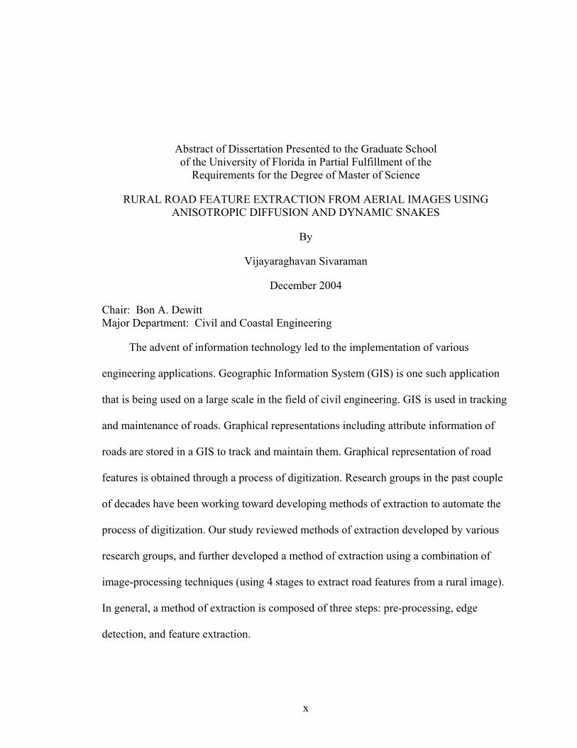
The advent of information technology led to the implementation of various
engineering applications. Geographic Information System (GIS) is one such application
that is being used on a large scale in the field of civil engineering. GIS is used in tracking
and maintenance of roads. Graphical representations including attribute information of
roads are stored in a GIS to track and maintain them. Graphical representation of road
features is obtained through a process of digitization. Research groups in the past couple
of decades have been working toward developing methods of extraction to automate the
process of digitization. Our study reviewed methods of extraction developed by various
research groups, and further developed a method of extraction using a combination of
image-processing techniques (using 4 stages to extract road features from a rural image).
In general, a method of extraction is composed of three steps: pre-processing, edge
detection, and feature extraction.
xi
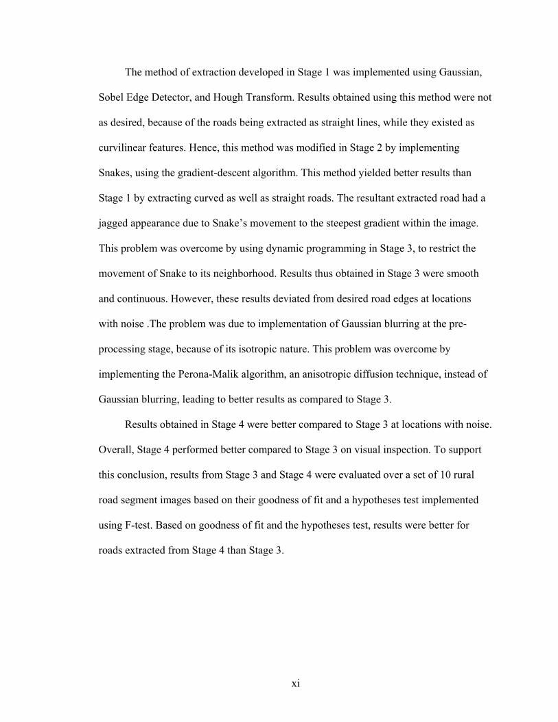
The method of extraction developed in Stage 1 was implemented using Gaussian,
Sobel Edge Detector, and Hough Transform. Results obtained using this method were not
as desired, because of the roads being extracted as straight lines, while they existed as
curvilinear features. Hence, this method was modified in Stage 2 by implementing
Snakes, using the gradient-descent algorithm. This method yielded better results than
Stage 1 by extracting curved as well as straight roads. The resultant extracted road had a
jagged appearance due to Snake’s movement to the steepest gradient within the image.
This problem was overcome by using dynamic programming in Stage 3, to restrict the
movement of Snake to its neighborhood. Results thus obtained in Stage 3 were smooth
and continuous. However, these results deviated from desired road edges at locations
with noise .The problem was due to implementation of Gaussian blurring at the pre-
processing stage, because of its isotropic nature. This problem was overcome by
implementing the Perona-Malik algorithm, an anisotropic diffusion technique, instead of
Gaussian blurring, leading to better results as compared to Stage 3.
Results obtained in Stage 4 were better compared to Stage 3 at locations with noise.
Overall, Stage 4 performed better compared to Stage 3 on visual inspection. To support
this conclusion, results from Stage 3 and Stage 4 were evaluated over a set of 10 rural
road segment images based on their goodness of fit and a hypotheses test implemented
using F-test. Based on goodness of fit and the hypotheses test, results were better for
roads extracted from Stage 4 than Stage 3.
1
CHAPTER 1 INTRODUCTION
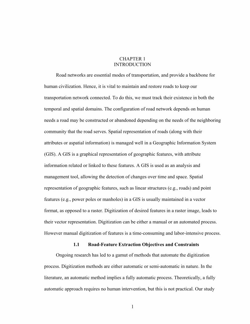
Road networks are essential modes of transportation, and provide a backbone for
human civilization. Hence, it is vital to maintain and restore roads to keep our
transportation network connected. To do this, we must track their existence in both the
temporal and spatial domains. The configuration of road network depends on human
needs a road may be constructed or abandoned depending on the needs of the neighboring
community that the road serves. Spatial representation of roads (along with their
attributes or aspatial information) is managed well in a Geographic Information System
(GIS). A GIS is a graphical representation of geographic features, with attribute
information related or linked to these features. A GIS is used as an analysis and
management tool, allowing the detection of changes over time and space. Spatial
representation of geographic features, such as linear structures (e.g., roads) and point
features (e.g., power poles or manholes) in a GIS is usually maintained in a vector
format, as opposed to a raster. Digitization of desired features in a raster image, leads to
their vector representation. Digitization can be either a manual or an automated process.
However manual digitization of features is a time-consuming and labor-intensive process.
1.1 Road-Feature Extraction Objectives and Constraints
Ongoing research has led to a gamut of methods that automate the digitization
process. Digitization methods are either automatic or semi-automatic in nature. In the
literature, an automatic method implies a fully automatic process. Theoretically, a fully
automatic approach requires no human intervention, but this is not practical. Our study
2
considered a method automatic if no human intervention was needed for road feature
extraction at the initial or processing stage. In a semi-automatic method human
intervention is required at the initial stage and at times during the processing stage. In
both methods, human intervention is needed at the post-processing stage. Post-processing
intervention is essential in both methods, to extract undetected but desired features from
the raster image, and to fix incorrectly extracted features. An automatic method scores
over a semi-automatic method due to its ability to automate the operations of the
initiation and processing stages. Road feature extraction from a raster image is a non-
trivial and image-specific process; hence, it is difficult to have one general method to
extract roads from any given raster image.
According to McKeown (1996), roads extracted from one raster image need not be
extracted in the same way from another raster image, as there can be a drastic change in
the value of important parameters based on nature’s state, instrument variation, and
photographic orientation. The existence of other features, both cultural (e.g., buildings)
and natural (e.g., trees) and their shadows can occlude road features, thus complicating
the extraction process. This ancillary information provides a context for many of the
approaches developed (Section 2.3.2). Thus, it is necessary to evaluate the extent of
inclusion of other information needed to identify a road. Some extraction cases need
minimal ancillary information; and some need a great deal. These limitations point to a
need to develop a method to evaluate multiple criteria in detecting and extracting roads
from images.
Our study extracted roads solely based on the road characteristics stored in an
implicit manner in a raster image. Parameters used for extraction are its shape (geometric
3
property) and gray-level intensity (radiometric property). These purely image-based
characteristics are affected by external sources as discussed earlier. No contextual
information was used. The method works solely on image characteristics. The method is
semi-automatic, with manual selection of the start and end of road segments in the input
image. Future work is needed to automate the initiation process, to automate the road
selection process, using Kalman Filter and profile matching processes (Appendix B).
1.2 Feature Extraction from a Geomatics Perspective
Feature extraction spans many applications, ranging from the field of medical
imaging to transportation and beyond. In Geomatics and Civil Engineering, the need for
feature extraction is project-oriented. For example, extracting features from an aerial
image is dependent on project needs; the goal may vary from detecting canopies of trees
to detecting manholes. The ability to classify and differentiate the desired features in an
aerial image is a critical step toward automating the extraction process. Difficulties faced
in the implementation of extraction methods are due to the complexity of the varied
information stored in an aerial image. A good extraction technique must be capable of
accurately determining the locations of necessary features in the image. Detection of a
feature object, and its extraction from an image, depends on its geometric, topologic, and
radiometric characteristics (Section 2.2).
4
CHAPTER 2 BACKGROUND
Road-feature extraction was studied from aerial images over the past 2 decades.
Numerous methods have been developed to extract road features from an aerial image.
Road feature extraction from an aerial image depends on characteristics of roads, and
their variations due to external factors (man-made and natural objects). A method of
extraction is broadly classified into three steps: pre-processing, edge-detection, and
feature extraction (initialized by a feature identification step). The efficiency of a given
method depends on image resolution and the input road characteristics (Section 2.1), and
also on the algorithms used (developed to extract the desired information, using a
combination of appropriate image-processing techniques). The task is to extract identified
road features that are explicit in nature and visually identifiable to a human, from implicit
information stored in the form of a matrix of values representing either gray levels or
color information in a raster image.
Digital raster images are portrayals of scenes, with imperfect renditions of objects
(Wolf and Dewitt, 2000). Imperfections in an image result from the imaging system,
signal noise, atmospheric scatter, and shadows. Thus, the task of identifying and
extracting the desired information or features from a raster image is based on criteria
developed to determine a particular feature (based on its characteristics within any raster
image), while ignoring the presence of other features and imperfections in the image
(Section 2.2).
5
Methods of extraction developed in past research are broadly classified into Semi-
automatic methods of extraction, or Automatic methods of extraction. Automatic
methods of extraction are more complex than Semi-automatic methods of extraction.
Automatic methods of extraction require ancillary information (Section 1.1), as compared
to Semi-automatic methods that extract roads based on information from the input image.
As part of a literature survey, Section 2.3 explains a Semi-automatic method of extraction
in detail, developed by Shukla et al. (2002), and an Automatic method of extraction,
developed by Baumgartner et al. (1999) from various methods developed in this field of
research
2.1 Road Characteristics
An aerial image is usually composed of numerous features, both man-made (e.g.,
buildings, roads) and natural (e.g., forests, vegetation) besides roads. Roads in an aerial
image can be represented based on the following characteristics: radiometric, geometric,
topologic, functional, and contextual, as is explained in detail later in this section. Factors
such as intensity of light, weather, and orientation of the camera can affect the
representation of the road features in an image based on the afore-mentioned
characteristics. This in turn affects the road extraction process. Geometric and
radiometric properties of a road are usually used as initial input characteristics in
determining road edge features. Both cultural and natural features can also be used as
contextual information to extract roads, along with external data apart from the
information in the image (geometric and radiometric characteristics). Contextual
information, and information from external sources, can be used to develop topologic,
functional, and contextual characteristics. Automatic method of extraction, implemented

6
by Baumgartner et al. (1999), use these characteristics, explained in detail in Section
2.3.2.
Human perceptual ways of recognizing a road come from looking at the geometric,
radiometric, topological, functional, and contextual characteristics of an image. For
example in Figure 2-1, a human will first recognize a road based on its geometric
characteristics, considering a road to be a long, elongated feature with constant width and
uniform radiometric variance along its length. As shown in Figure 2-1, Road 1 and Road
2 have different overall pixel intensities (a radiometric property) and widths (a geometric
property). However, both tend to exist as long continuous features.
Thus, it is up to the discretion of the user to select appropriate roads to be extracted
at the feature-identification step. If the feature-identification step is automated, the
program needs to be trained to select roads based on radiometric variance that varies
depending on the functional characteristics of a road; explained later in this section. As
an example in Figure 2-1, Road 1 and Road 2 have different functional properties and
have different radiometric representations. In the case if a human is unable to locate a
road segment due to occlusion, because of a tree (Figure 2-1) or a car, a human would use
contextual information or topological characteristics. Existence of trees or
buildings/houses in the vicinity is used as contextual information. Where as, topologic
properties of the roads are used to determine the missing segment of the road network.
Thus to automate the process of determining the presence of a road, there is a need to
develop a technique for extracting roads, using cues that humans would use, to give the
system the ability to determine and extract the roads in an aerial image based on the
characteristics of a road described.
7
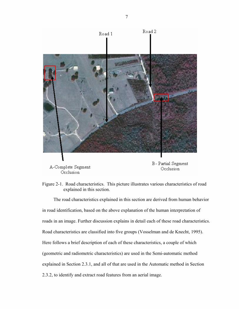
Figure 2-1. Road characteristics. This picture illustrates various characteristics of road
explained in this section.
The road characteristics explained in this section are derived from human behavior
in road identification, based on the above explanation of the human interpretation of
roads in an image. Further discussion explains in detail each of these road characteristics.
Road characteristics are classified into five groups (Vosselman and de Knecht, 1995).
Here follows a brief description of each of these characteristics, a couple of which
(geometric and radiometric characteristics) are used in the Semi-automatic method
explained in Section 2.3.1, and all of that are used in the Automatic method in Section
2.3.2, to identify and extract road features from an aerial image.
8
2.1.1 Geometric
Roads are elongated, and in high-resolution aerial images they run through the
image as long parallel edges with a constant width and curvature. Constraints on
detection based purely on such characteristics comes from the fact that there are other
features, like rivers that may be misclassified as roads, if an automated procedure to
identify road segments is implemented in an extraction method. This leads to a
requirement for the use of additional characteristics when extracting roads. In addition,
roads within an image may have different widths, based on their functional classification.
In Figure 2-1, Road 1 and Road 2 have different widths, because of their functional
characteristics, they are a local road and a highway respectively, this issue is discussed in
Section 2.1.4. Thus, this characteristic alone cannot be used as a parameter in the
automatic extraction of a road from an aerial image.
2.1.2 Radiometric
A road surface is homogenous and often has a good level of contrast with adjacent
areas. Thus, radiometric properties, or overall intensity values, of a road segment remain
nearly uniform through the road in an image. A road’s radiometric properties, as a
parameter in road characterization, identifies a road segment to be part of a road, based
on its overall intensity value when compared to a model, or other road segments forming
the road network in the image. This works well in most cases, with the exception of areas
where buildings or trees occlude the road or the presence of cars affects the feature
detection process using this characteristic. It also varies with the weather and orientation
of the camera at the time of exposure. For example, in Figure 2-1, A illustrates the
complete occlusion of a road segment and B illustrates the partial occlusion of a road
segment due to the trees near the occluded road segment.
9
A method of extraction based on radiometric properties may not identify segments
A and B (Figure 2-1), due to its inability to match the occluded road segment with the
other road segments in the image based purely on its radiometric property. Since the
radiometric characteristics of the occluded road segments would be very different from
those of the un-occluded road segments in the image. In addition, if the process of
identification is automated, and if the program is not trained to deal with different
pavement types, detection would get affected, since an asphalt road surface may have
different road characteristics to a tar road. Hence, a group of characteristics used together
would better identify a road segment, as compared to identification based on individual
characteristics.
2.1.3 Topologic
Topologic characteristics of roads are based on the ability of roads to form road
networks with intersections/junctions, and terminations at points of interest (e.g.,
Apartment, Buildings, Agricultural lands). Roads generally tend to connect regions or
centers of activity in an aerial image; they may begin at a building (e.g., house) in Figure
2-1 and terminate at another center of activity, or continue to end of an image. Roads tend
to intersect and to connect to the other roads in an image. Topological information, as
explained above, can be used to identify and extract missing segments of roads. As an
example, if we have to extract the roads from the image in Figure 2-1, the radiometric
and geometric characteristics of the road would help to extract all the road segments in
the image. Though, it won’t be able to extract certain segments, due to shadow occlusion
A or the presence of cars and buildings B in the vicinity (Figure 2-1). These missing or
occluded road segments could be linked to the extracted segments based on the
topological information of the neighboring segments. This characteristic is used in the
10
automatic method of extraction developed by Baumgartner et al. (1999) as explained in
detail later in this chapter (Section 2.3.2).
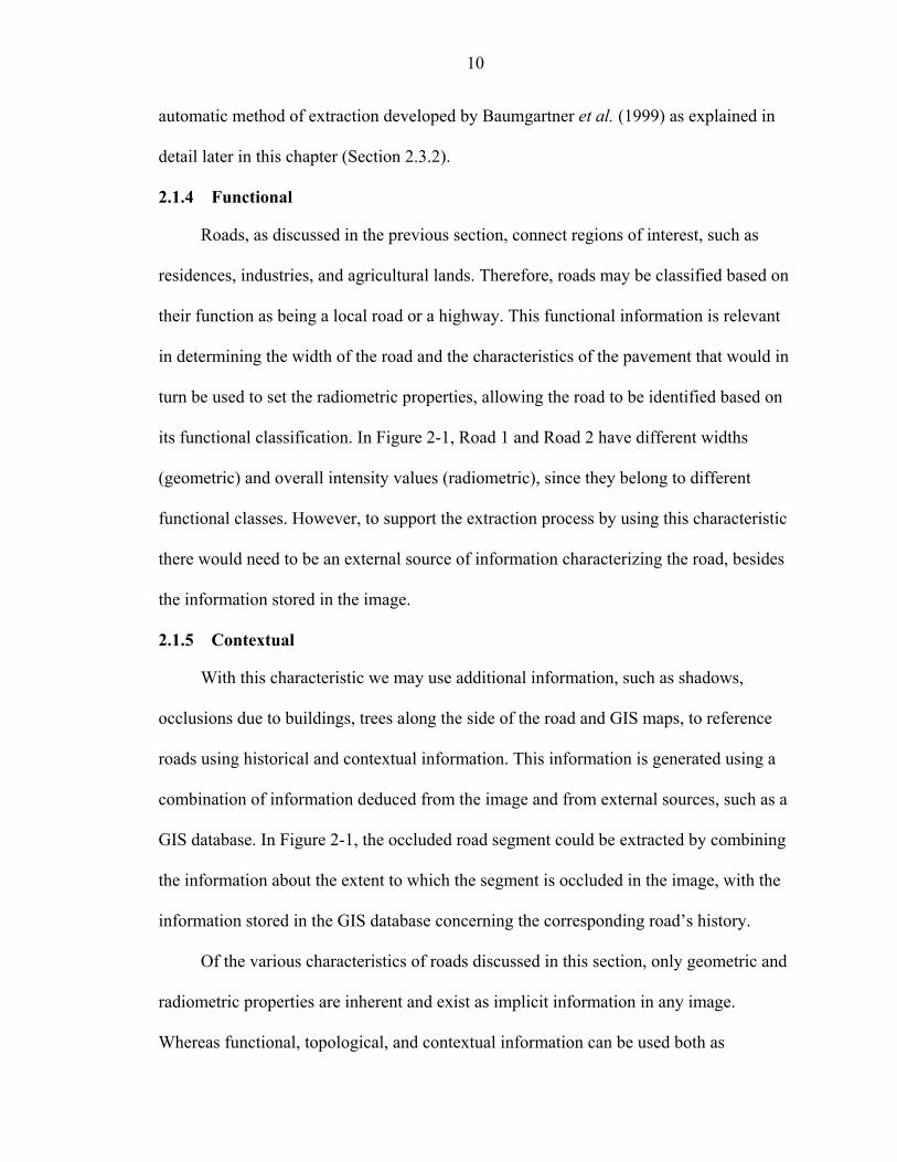
2.1.4 Functional
Roads, as discussed in the previous section, connect regions of interest, such as
residences, industries, and agricultural lands. Therefore, roads may be classified based on
their function as being a local road or a highway. This functional information is relevant
in determining the width of the road and the characteristics of the pavement that would in
turn be used to set the radiometric properties, allowing the road to be identified based on
its functional classification. In Figure 2-1, Road 1 and Road 2 have different widths
(geometric) and overall intensity values (radiometric), since they belong to different
functional classes. However, to support the extraction process by using this characteristic
there would need to be an external source of information characterizing the road, besides
the information stored in the image.
2.1.5 Contextual
With this characteristic we may use additional information, such as shadows,
occlusions due to buildings, trees along the side of the road and GIS maps, to reference
roads using historical and contextual information. This information is generated using a
combination of information deduced from the image and from external sources, such as a
GIS database. In Figure 2-1, the occluded road segment could be extracted by combining
the information about the extent to which the segment is occluded in the image, with the
information stored in the GIS database concerning the corresponding road’s history.
Of the various characteristics of roads discussed in this section, only geometric and
radiometric properties are inherent and exist as implicit information in any image.
Whereas functional, topological, and contextual information can be used both as
11
information from the image and from an external data source, to develop an intelligent
approach to the identification and extraction of occluded and missing road segments in
the image. The Semi-automatic method explained in section 2.3.1 illustrates the use of
the geometric and radiometric properties of a road as input information for the extraction
of road features technique that was implemented by Shukla et al. (2002). Furthermore, in
Section 2.3.2, the Automatic method implemented by Baumgartner et al. (1999)
illustrates an extraction process, where the initial extraction process is carried out using
the geometric and radiometric characteristics of the road in an image, supported by
extraction using topologic, functional, and contextual characteristics.
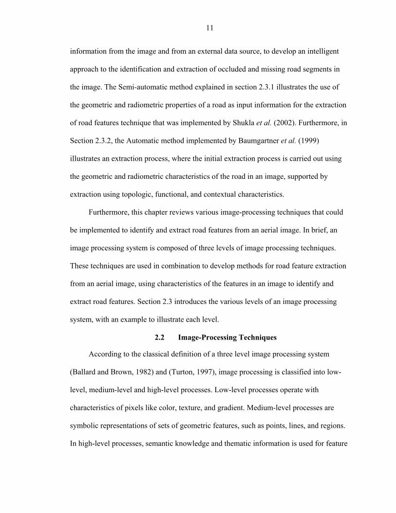
Furthermore, this chapter reviews various image-processing techniques that could
be implemented to identify and extract road features from an aerial image. In brief, an
image processing system is composed of three levels of image processing techniques.
These techniques are used in combination to develop methods for road feature extraction
from an aerial image, using characteristics of the features in an image to identify and
extract road features. Section 2.3 introduces the various levels of an image processing
system, with an example to illustrate each level.
2.2 Image-Processing Techniques
According to the classical definition of a three level image processing system
(Ballard and Brown, 1982) and (Turton, 1997), image processing is classified into low-
level, medium-level and high-level processes. Low-level processes operate with
characteristics of pixels like color, texture, and gradient. Medium-level processes are
symbolic representations of sets of geometric features, such as points, lines, and regions.
In high-level processes, semantic knowledge and thematic information is used for feature

12
extraction. Sections 2.3.1 through 2.3.3 explain various levels of image processing, with
an illustration from each level, explaining a technique and its implementation.
2.2.1 Low-Level Processing
This step is concerned with cleaning and minimizing noise (i.e., pixels with an
intensity value different from the average intensity value of the relevant region within an
image) in the image, before further operations can be carried out to extract the desired
information from the image. One of simplest Low-Level processes is to blur an image by
averaging the values of the pixels forming the image, thereby minimizing noise; here a
mean or an average value is calculated for a group of pixel values forming an image,
thereby reducing the variation in intensity between the pixels in the image.
Table 2-1. Image pixel subset 2 3 3 3 2
4 2 3 4 4
5 2 3 4 5
3 6 6 4 4
Image pixel subset represents an image, with red values representing the pixels considered for convolution using Table 2-2 explained in this section. Table 2-2. Convolution kernel 1/9 1/9 1/9
1/9 1/9 1/9
1/9 1/9 1/9
Convolution kernel is convolved through the image whose pixel values are represented in Table 2-1, convolution of Table 2-2 with pixel subset highlighted in red in Table 2-1 is explained in this section.
13
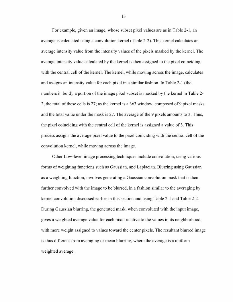
For example, given an image, whose subset pixel values are as in Table 2-1, an
average is calculated using a convolution kernel (Table 2-2). This kernel calculates an
average intensity value from the intensity values of the pixels masked by the kernel. The
average intensity value calculated by the kernel is then assigned to the pixel coinciding
with the central cell of the kernel. The kernel, while moving across the image, calculates
and assigns an intensity value for each pixel in a similar fashion. In Table 2-1 (the
numbers in bold), a portion of the image pixel subset is masked by the kernel in Table 2-
2, the total of these cells is 27; as the kernel is a 3x3 window, composed of 9 pixel masks
and the total value under the mask is 27. The average of the 9 pixels amounts to 3. Thus,
the pixel coinciding with the central cell of the kernel is assigned a value of 3. This
process assigns the average pixel value to the pixel coinciding with the central cell of the
convolution kernel, while moving across the image.
Other Low-level image processing techniques include convolution, using various
forms of weighting functions such as Gaussian, and Laplacian. Blurring using Gaussian
as a weighting function, involves generating a Gaussian convolution mask that is then
further convolved with the image to be blurred, in a fashion similar to the averaging by
kernel convolution discussed earlier in this section and using Table 2-1 and Table 2-2.
During Gaussian blurring, the generated mask, when convoluted with the input image,
gives a weighted average value for each pixel relative to the values in its neighborhood,
with more weight assigned to values toward the center pixels. The resultant blurred image
is thus different from averaging or mean blurring, where the average is a uniform
weighted average.
14
22
22
21),( 2
σσ
yx
eyxG
+
Π=
−
(2-1)
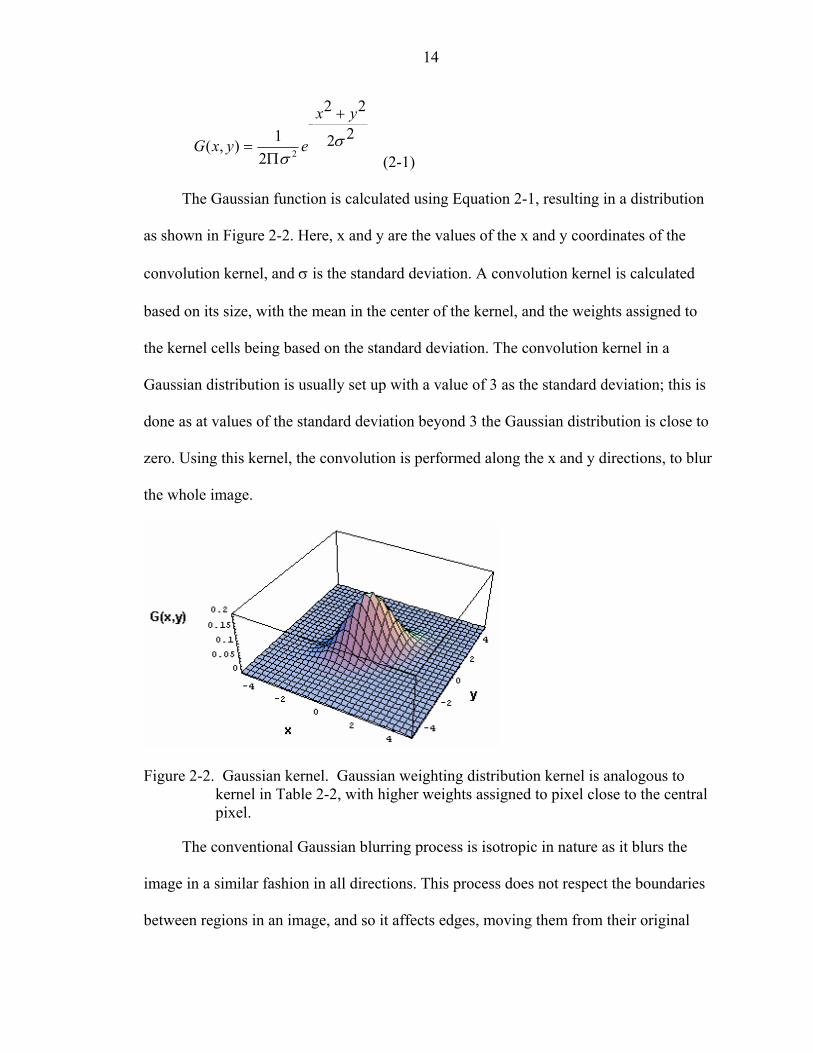
The Gaussian function is calculated using Equation 2-1, resulting in a distribution
as shown in Figure 2-2. Here, x and y are the values of the x and y coordinates of the
convolution kernel, and σ is the standard deviation. A convolution kernel is calculated
based on its size, with the mean in the center of the kernel, and the weights assigned to
the kernel cells being based on the standard deviation. The convolution kernel in a
Gaussian distribution is usually set up with a value of 3 as the standard deviation; this is
done as at values of the standard deviation beyond 3 the Gaussian distribution is close to
zero. Using this kernel, the convolution is performed along the x and y directions, to blur
the whole image.
Figure 2-2. Gaussian kernel. Gaussian weighting distribution kernel is analogous to
kernel in Table 2-2, with higher weights assigned to pixel close to the central pixel.
The conventional Gaussian blurring process is isotropic in nature as it blurs the
image in a similar fashion in all directions. This process does not respect the boundaries
between regions in an image, and so it affects edges, moving them from their original
15
position. Hence, in our study the Perona-Malik algorithm (Malik and Perona, 1990), is
implemented, an anisotropic diffusion principle to blur an image, in the developed
method of extraction, instead of the conventional blurring process using a Gaussian. In
the Perona-Malik algorithm images are blurred within regions, while the edges are kept
intact and enhanced, preserving the boundaries between regions. Chapter 3 introduces the
principle of isotropic and anisotropic diffusion in Section 3.1, and its implementation in
the Perona-Malik algorithm, in Section 3.2.
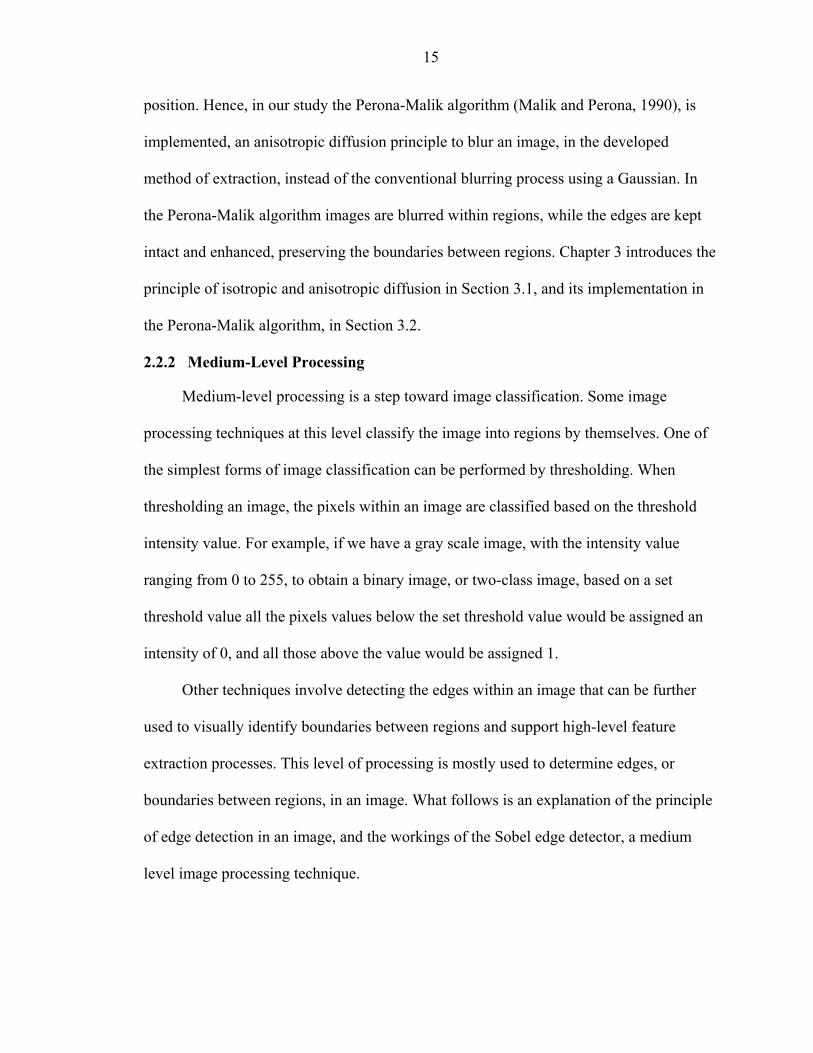
2.2.2 Medium-Level Processing
Medium-level processing is a step toward image classification. Some image
processing techniques at this level classify the image into regions by themselves. One of
the simplest forms of image classification can be performed by thresholding. When
thresholding an image, the pixels within an image are classified based on the threshold
intensity value. For example, if we have a gray scale image, with the intensity value
ranging from 0 to 255, to obtain a binary image, or two-class image, based on a set
threshold value all the pixels values below the set threshold value would be assigned an
intensity of 0, and all those above the value would be assigned 1.
Other techniques involve detecting the edges within an image that can be further
used to visually identify boundaries between regions and support high-level feature
extraction processes. This level of processing is mostly used to determine edges, or
boundaries between regions, in an image. What follows is an explanation of the principle
of edge detection in an image, and the workings of the Sobel edge detector, a medium
level image processing technique.
16
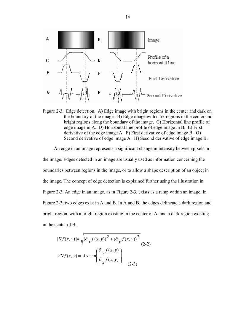
Figure 2-3. Edge detection. A) Edge image with bright regions in the center and dark on
the boundary of the image. B) Edge image with dark regions in the center and bright regions along the boundary of the image. C) Horizontal line profile of edge image in A. D) Horizontal line profile of edge image in B. E) First derivative of the edge image A. F) First derivative of edge image B. G) Second derivative of edge image A. H) Second derivative of edge image B.
An edge in an image represents a significant change in intensity between pixels in
the image. Edges detected in an image are usually used as information concerning the
boundaries between regions in the image, or to allow a shape description of an object in
the image. The concept of edge detection is explained further using the illustration in
Figure 2-3. An edge in an image, as in Figure 2-3, exists as a ramp within an image. In
Figure 2-3, two edges exist in A and B. In A and B, the edges delineate a dark region and
bright region, with a bright region existing in the center of A, and a dark region existing
in the center of B.
2)),((2)),((|),(| yxfyyxfxyxf ∂+∂=∇
(2-2)
∂
∂=∠∇
),(
),(tan),(
yxfx
yxfyArcyxf
(2-3)
17
A and B in Figure 2-3, are considered to be continuous along x and y, ),( yxf then
represents the image. Derivatives along the x (),( yxfx∂ ) and y directions (
),( yxfy∂ ),
also known as directional derivatives, are calculated from the input image. Edges within
the image are determined based on Equation 2-2 and Equation 2-3 that are calculated
using the directional derivatives. Equation 2-2 gives the magnitude of the gradient and
Equation 2-3 gives the orientation of the gradient.
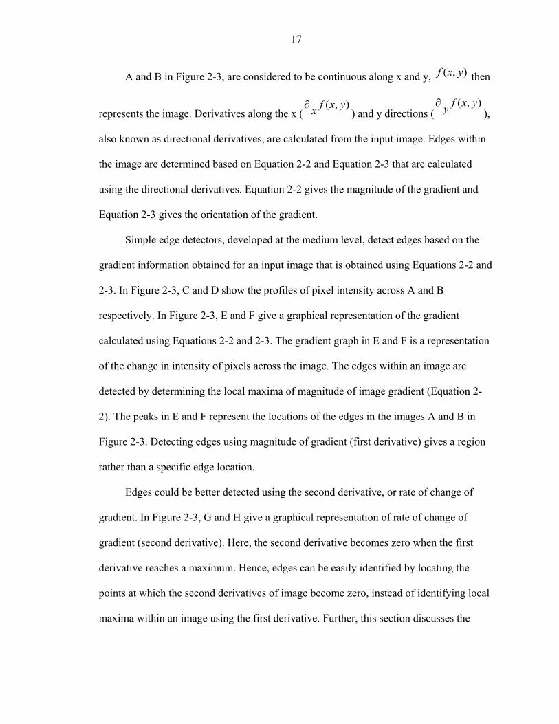
Simple edge detectors, developed at the medium level, detect edges based on the
gradient information obtained for an input image that is obtained using Equations 2-2 and
2-3. In Figure 2-3, C and D show the profiles of pixel intensity across A and B
respectively. In Figure 2-3, E and F give a graphical representation of the gradient
calculated using Equations 2-2 and 2-3. The gradient graph in E and F is a representation
of the change in intensity of pixels across the image. The edges within an image are
detected by determining the local maxima of magnitude of image gradient (Equation 2-
2). The peaks in E and F represent the locations of the edges in the images A and B in
Figure 2-3. Detecting edges using magnitude of gradient (first derivative) gives a region
rather than a specific edge location.
Edges could be better detected using the second derivative, or rate of change of
gradient. In Figure 2-3, G and H give a graphical representation of rate of change of
gradient (second derivative). Here, the second derivative becomes zero when the first
derivative reaches a maximum. Hence, edges can be easily identified by locating the
points at which the second derivatives of image become zero, instead of identifying local
maxima within an image using the first derivative. Further, this section discusses the
18
working a Sobel edge detector that performs gradient measurement and locates regions
with high gradients that correspond to edges within an image.
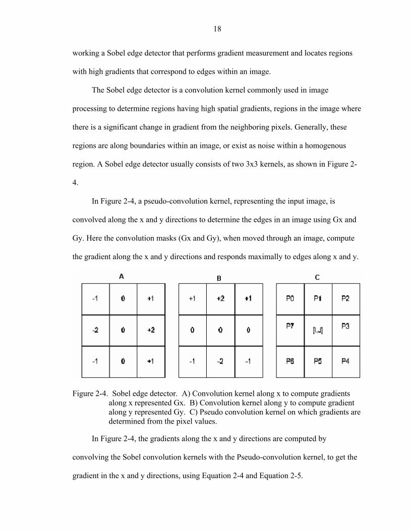
The Sobel edge detector is a convolution kernel commonly used in image
processing to determine regions having high spatial gradients, regions in the image where
there is a significant change in gradient from the neighboring pixels. Generally, these
regions are along boundaries within an image, or exist as noise within a homogenous
region. A Sobel edge detector usually consists of two 3x3 kernels, as shown in Figure 2-
4.
In Figure 2-4, a pseudo-convolution kernel, representing the input image, is
convolved along the x and y directions to determine the edges in an image using Gx and
Gy. Here the convolution masks (Gx and Gy), when moved through an image, compute
the gradient along the x and y directions and responds maximally to edges along x and y.
Figure 2-4. Sobel edge detector. A) Convolution kernel along x to compute gradients
along x represented Gx. B) Convolution kernel along y to compute gradient along y represented Gy. C) Pseudo convolution kernel on which gradients are determined from the pixel values.
In Figure 2-4, the gradients along the x and y directions are computed by
convolving the Sobel convolution kernels with the Pseudo-convolution kernel, to get the
gradient in the x and y directions, using Equation 2-4 and Equation 2-5.
19
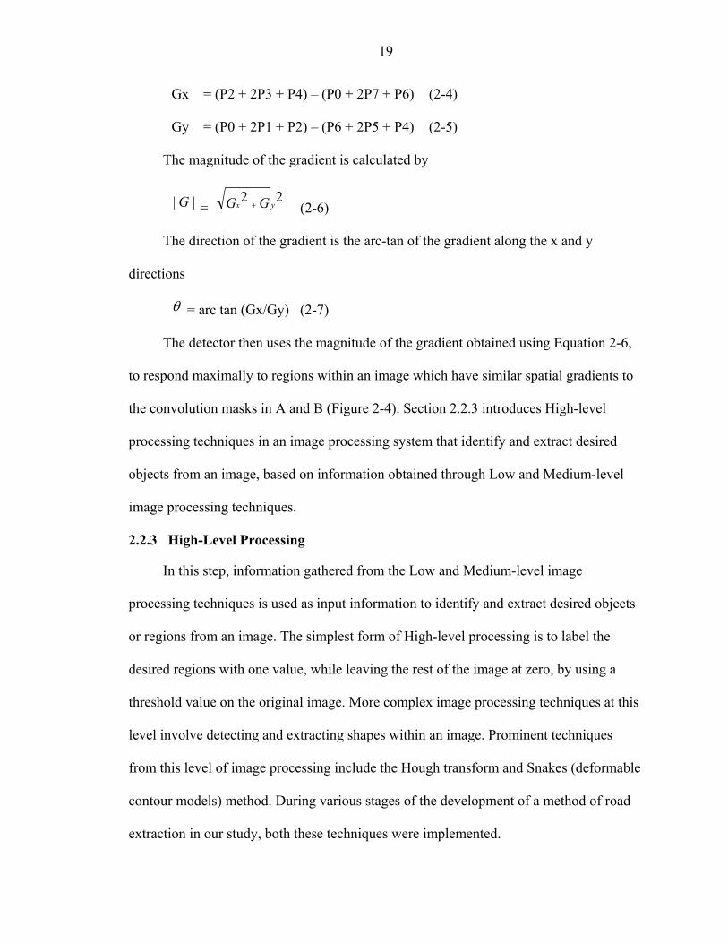
Gx = (P2 + 2P3 + P4) – (P0 + 2P7 + P6) (2-4)
Gy = (P0 + 2P1 + P2) – (P6 + 2P5 + P4) (2-5)
The magnitude of the gradient is calculated by
|| G = 22
yx GG + (2-6)
The direction of the gradient is the arc-tan of the gradient along the x and y
directions
θ = arc tan (Gx/Gy) (2-7)
The detector then uses the magnitude of the gradient obtained using Equation 2-6,
to respond maximally to regions within an image which have similar spatial gradients to
the convolution masks in A and B (Figure 2-4). Section 2.2.3 introduces High-level
processing techniques in an image processing system that identify and extract desired
objects from an image, based on information obtained through Low and Medium-level
image processing techniques.
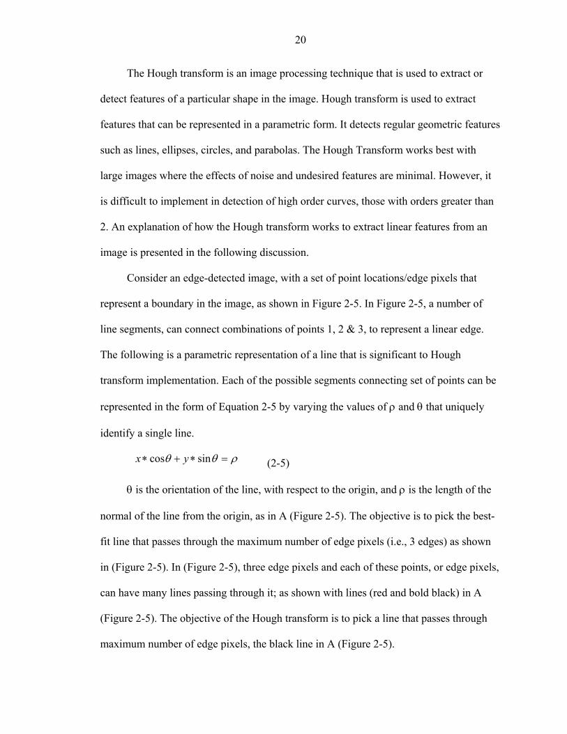
2.2.3 High-Level Processing
In this step, information gathered from the Low and Medium-level image
processing techniques is used as input information to identify and extract desired objects
or regions from an image. The simplest form of High-level processing is to label the
desired regions with one value, while leaving the rest of the image at zero, by using a
threshold value on the original image. More complex image processing techniques at this
level involve detecting and extracting shapes within an image. Prominent techniques
from this level of image processing include the Hough transform and Snakes (deformable
contour models) method. During various stages of the development of a method of road
extraction in our study, both these techniques were implemented.
20
The Hough transform is an image processing technique that is used to extract or
detect features of a particular shape in the image. Hough transform is used to extract
features that can be represented in a parametric form. It detects regular geometric features
such as lines, ellipses, circles, and parabolas. The Hough Transform works best with
large images where the effects of noise and undesired features are minimal. However, it
is difficult to implement in detection of high order curves, those with orders greater than
2. An explanation of how the Hough transform works to extract linear features from an
image is presented in the following discussion.
Consider an edge-detected image, with a set of point locations/edge pixels that
represent a boundary in the image, as shown in Figure 2-5. In Figure 2-5, a number of
line segments, can connect combinations of points 1, 2 & 3, to represent a linear edge.
The following is a parametric representation of a line that is significant to Hough
transform implementation. Each of the possible segments connecting set of points can be
represented in the form of Equation 2-5 by varying the values of ρ and θ that uniquely
identify a single line.
ρθθ =∗+∗ sincos yx (2-5)
θ is the orientation of the line, with respect to the origin, and ρ is the length of the
normal of the line from the origin, as in A (Figure 2-5). The objective is to pick the best-
fit line that passes through the maximum number of edge pixels (i.e., 3 edges) as shown
in (Figure 2-5). In (Figure 2-5), three edge pixels and each of these points, or edge pixels,
can have many lines passing through it; as shown with lines (red and bold black) in A
(Figure 2-5). The objective of the Hough transform is to pick a line that passes through
maximum number of edge pixels, the black line in A (Figure 2-5).
21
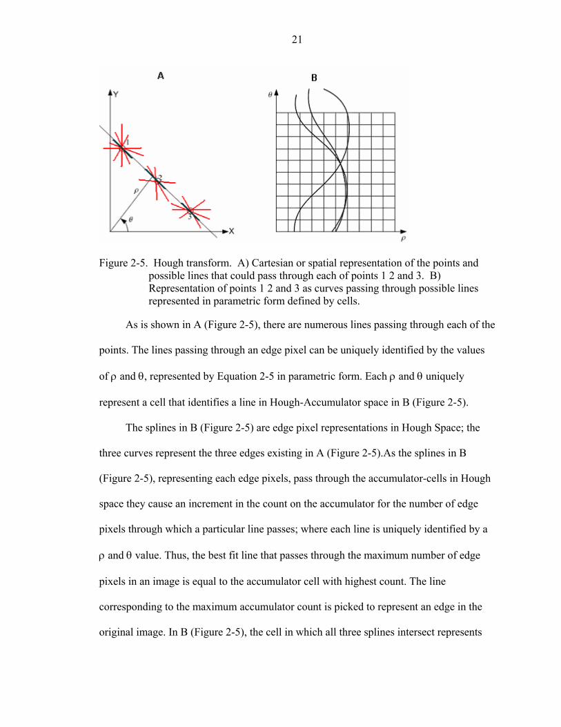
Figure 2-5. Hough transform. A) Cartesian or spatial representation of the points and
possible lines that could pass through each of points 1 2 and 3. B) Representation of points 1 2 and 3 as curves passing through possible lines represented in parametric form defined by cells.
As is shown in A (Figure 2-5), there are numerous lines passing through each of the
points. The lines passing through an edge pixel can be uniquely identified by the values
of ρ and θ, represented by Equation 2-5 in parametric form. Each ρ and θ uniquely
represent a cell that identifies a line in Hough-Accumulator space in B (Figure 2-5).
The splines in B (Figure 2-5) are edge pixel representations in Hough Space; the
three curves represent the three edges existing in A (Figure 2-5).As the splines in B
(Figure 2-5), representing each edge pixels, pass through the accumulator-cells in Hough
space they cause an increment in the count on the accumulator for the number of edge
pixels through which a particular line passes; where each line is uniquely identified by a
ρ and θ value. Thus, the best fit line that passes through the maximum number of edge
pixels in an image is equal to the accumulator cell with highest count. The line
corresponding to the maximum accumulator count is picked to represent an edge in the
original image. In B (Figure 2-5), the cell in which all three splines intersect represents
22
the cell with the highest count of edge pixels. Hence, it is considered to be the best-fit
line, and so the black line in representation of an edge in A (Figure 2-5).
During the initial stage of this research, an implementation of the Hough transform
to extract road features was attempted, but was not considered, as road features were
extracted from the image as straight lines; whereas roads typically exist as splines or
curvilinear features in an image. This led to the implementation of Snakes (Active
Contour model) to extract roads, as they represented road features better than Hough
lines.
Section 2.3 further introduces various methods of road feature extraction developed
over the past couple of decades. This section discusses in detail a Semi-Automatic and
Automatic approach to road feature extraction.
2.3 Approaches to Road Feature Extraction
There are numerous methods that have been developed to extract road features
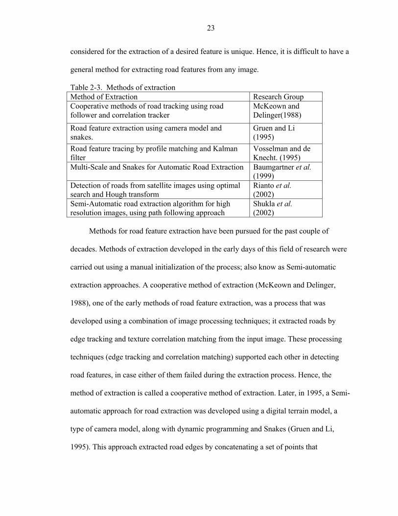
from an aerial image. Table 2-3 lists a few of the road extraction methods reviewed here,
as part of literature survey, prior to work beginning on the development of a method of
extraction in our study. Methods of extraction developed by researchers have been
developed using a combination of image processing techniques. Techniques implemented
in the methods of extraction may be common to one or more of the listed methods. Road
extraction methods are broadly classified into Semi-automatic approaches and Automatic
approaches, as was discussed in Section 1.1. The methods of extraction listed in Table 2-
3, include a group of Semi-automatic approaches, and an Automatic approach that was
developed by Baumgartner et al. (1999) According to McKeown (1996), one of the early
researchers involved in developing road feature extraction methods, every image
23
considered for the extraction of a desired feature is unique. Hence, it is difficult to have a
general method for extracting road features from any image.
Table 2-3. Methods of extraction Method of Extraction Research Group Cooperative methods of road tracking using road follower and correlation tracker
McKeown and Delinger(1988)
Road feature extraction using camera model and snakes.
Gruen and Li (1995)
Road feature tracing by profile matching and Kalman filter
Vosselman and de Knecht. (1995)
Multi-Scale and Snakes for Automatic Road Extraction Baumgartner et al. (1999)
Detection of roads from satellite images using optimal search and Hough transform
Rianto et al. (2002)
Semi-Automatic road extraction algorithm for high resolution images, using path following approach
Shukla et al. (2002)
Methods for road feature extraction have been pursued for the past couple of
decades. Methods of extraction developed in the early days of this field of research were
carried out using a manual initialization of the process; also know as Semi-automatic
extraction approaches. A cooperative method of extraction (McKeown and Delinger,
1988), one of the early methods of road feature extraction, was a process that was
developed using a combination of image processing techniques; it extracted roads by
edge tracking and texture correlation matching from the input image. These processing
techniques (edge tracking and correlation matching) supported each other in detecting
road features, in case either of them failed during the extraction process. Hence, the
method of extraction is called a cooperative method of extraction. Later, in 1995, a Semi-
automatic approach for road extraction was developed using a digital terrain model, a
type of camera model, along with dynamic programming and Snakes (Gruen and Li,
1995). This approach extracted road edges by concatenating a set of points that
24
represented road locations. Another Semi-automatic approach was developed around the
same time, and extracted road features using the Kalman filter and profile matching
(Vosselman and de Knecht, 1995). During the evolution of the various methods of road
feature extraction, a research group lead by Baumgartner et al. (1999) developed an
Automatic approach. Most of methods developed until this date had the similar extraction
steps, but this method tried and tested a different combination of image processing
techniques to work in cooperation with each other in modules. Our study will discuss
further a Semi-automatic method of extraction, a Semi-automatic road extraction
algorithm for high-resolution images using the path following approach (Shukla et al.
2002), and an Automatic method of extraction, the Multi-scale and Snakes road feature
extraction method developed by Baumgartner et al. (1999).
Furthermore, a method of extraction is developed in our study that uses a
combination of image processing techniques, evolved over stages that use cues from past
research to develop a method of road feature extraction. An initial attempt was made to
extract roads using the Hough Transform based on a concept from method of extraction
developed by Rianto et al. (2002), although the results obtained were not as desired.
Hence , many combinations were tested, the final method of extraction that will be
implemented in our study uses the Perona-Malik algorithm (Malik and Perona, 1990),
based on the anisotropic diffusion principle and Snakes, was developed at final stage,
stage 4 (Section 5.1). As part of our study, an attempt was made to automate the
initialization, or road segment identification, stage prior to extraction (Section 5.2.1)
using the Kalman Filter and profile matching (Vosselman and de Knecht, 1995).
Appendix B of our study gives a detailed explanation of the principle and working of the
25
Kalman Filter, along with its implementation for detecting road segments using profile
matching and Kalman filter. Furthermore, Sections 2.3.1 and 2.3.2 explain in detail the
methods of extraction that were developed by Shukla et al. (2002) and Baumgartner et al.
(1999), each under the Semi-automatic and Automatic approaches to road feature
extraction respectively.
Prior to discussing and evaluating the approaches that have been developed toward
road feature extraction from an aerial image, there is some information to be dealt with
concerning the general observation of a road. Roads are generally uniform in width in
high-resolution images, and appear as lines in low-resolution images, depending on the
resolution of the image and functional classification of the road. In the Automatic
approach discussed below, road features are extracted at various resolutions using
contextual information to complete the extraction of roads from an input aerial image. In
both approaches (Automatic and Semi-automatic), there is a need for human intervention
at some point during the extraction process. A Semi-automatic approach requires initial
human intervention, and at times it requires intervention during the extraction process,
whereas an Automatic approach only needs human intervention at the post processing
stage. In the Semi-automatic approach, road detection is initialized manually with points
representing roads, also called seed points. The roads are tracked using these seed points
as an initial estimation of road feature identifiers. In the case of a fully Automatic
approach, the roads are completely extracted without any human intervention. Post
processing is carried out for misidentified and unidentified roads in both approaches.
2.3.1 Road Extraction Algorithm Using a Path-Following Approach
A Semi-automatic method is usually implemented using one of the techniques
below.
26
• Post initialization of the road, the road is mapped using a road tracing algorithm.
• Distribution of a sparse set of points along a road segment which are then concatenated to extract the desired road segment.
McKeown and Delinger (1988) developed a method by which to track and trace
roads in an aerial image, using an edge detector and texture correlation information
(Table 2-3). Whereas Gruen and Li (1995), implemented a road tracing technique using a
sparse set of points spaced along the road to be mapped using dynamic programming.
This section explains in detail a Semi-automatic method of extraction using path
following approach developed by Shukla et al. (2002).
In the method developed using path following approach, a road extraction
algorithm extracts roads using the width and variance information of a road segment,
obtained through the pre-processing and edge detection steps, similar to McKeown and
Delinger (1988) and Vosselman and de Knecht (1995). This process, being a Semi-
automatic approach, is initialized by a selection of a minimum of two road seed points.
These seed points are used to determine the center of the road programmatically from the
edge-detected image. Then, after the desired points representing the initial road segment
are obtained, its orientation and width are calculated. The orientation of the initial seed
point is used to determine the three directions along which the next road segment could
exist. From the three directions, the direction having minimum cost, (i.e., having the
minimum variance based on intensity or radiometric information) is considered as the
next road segment. This process is carried out iteratively, until the cost remains within the
predefined variance value. Below is a detailed systematic explanation of this approach.
Figure 2-6, gives a flow diagram of the extraction process, developed using the path
following approach (Shukla et al. 2002).
27
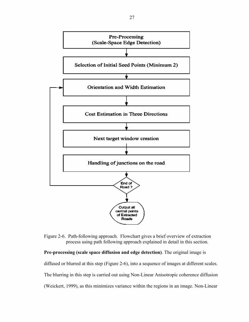
Figure 2-6. Path-following approach. Flowchart gives a brief overview of extraction
process using path following approach explained in detail in this section.
Pre-processing (scale space diffusion and edge detection). The original image is
diffused or blurred at this step (Figure 2-6), into a sequence of images at different scales.
The blurring in this step is carried out using Non-Linear Anisotropic coherence diffusion
(Weickert, 1999), as this minimizes variance within the regions in an image. Non-Linear
28
Anisotropic coherence diffusion helps maintain the homogeneity of regions within an
image. Variance across sections of the road segment is then further used to estimate the
cost, based on which road is traced. The anisotropic diffusion approach is a non-uniform
blurring technique, as it blurs regions within an image based on pre-defined criteria. This
is different to Gaussian blurring that blurs in a similar manner across the entire image.
The image diffused using the above diffusion technique is then used to compute the
radiometric variance across the pixels in the image. Edges are then detected from the
diffused image using a canny edge detector. The edge-detected image is used to calculate
the width of the road across road segments later in the process of extracting road
segments.
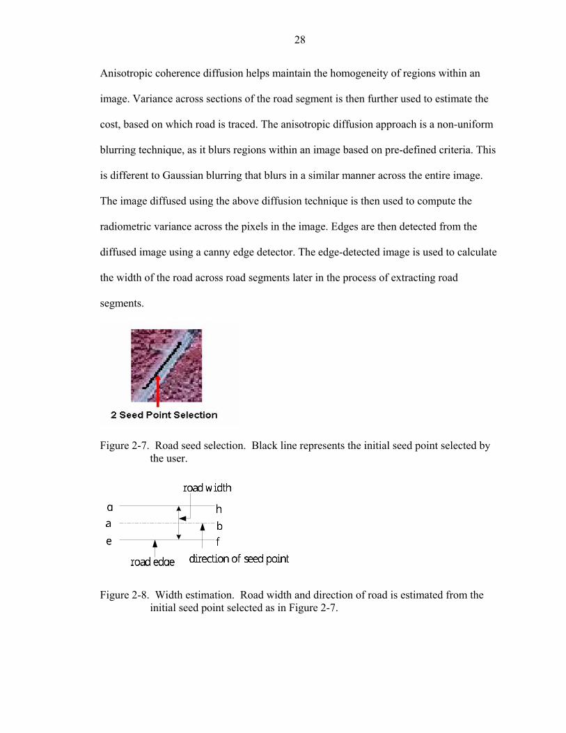
Figure 2-7. Road seed selection. Black line represents the initial seed point selected by
the user.
Figure 2-8. Width estimation. Road width and direction of road is estimated from the
initial seed point selected as in Figure 2-7.
Rajesh Chaudhary
road width
Rajesh Chaudhary
g
Rajesh Chaudhary
h
Rajesh Chaudhary
e
Rajesh Chaudhary
f
Rajesh Chaudhary
a
Rajesh Chaudhary
b
Rajesh Chaudhary
road edge
Rajesh Chaudhary
direction of seed point
29
Selection of initial seed points. As this algorithm is a Semi-automatic approach to
road feature extraction, the process of detecting and extracting road segments is
initialized by manual selection of road seed points. Road seed points, as in (Figure 2-7),
are two points on or near a road segment in an image that form a line segment
representing the road to be extracted selected by the user. (Figure 2-8) illustrates a road
seed with ends a and b. Comparing (Figure 2-7) and (Figure 2-8), a-b correspond to the
end points for the black road seed in (Figure 2-7).
Orientation and width estimation. In (Figure 2-8), a-b the current seed point’s
orientation gives the direction of the road, on the basis of which the rest of the road
segments could be determined. The width of the road at the given seed point is estimated
by calculating the distance from the parallel edges, g-h and e-f, to the road seeds a-b as in
(Figure 2-8). At this point the width of the road at the initial seed points is estimated,
along with the orientation of the road. The orientation of the road at the initial seed points
gives a lead as to three directions in which the road could propagate and form the next
road segment.
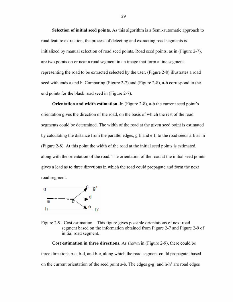
Figure 2-9. Cost estimation. This figure gives possible orientations of next road
segment based on the information obtained from Figure 2-7 and Figure 2-9 of initial road segment.
Cost estimation in three directions. As shown in (Figure 2-9), there could be
three directions b-c, b-d, and b-e, along which the road segment could propagate, based
on the current orientation of the seed point a-b. The edges g-g’ and h-h’ are road edges
30
parallel to the current road seed a-b. Thus if a-b is the current direction of the road
segment, b-c, b-d or b-e are the possible choices of direction for the next road segment.
As per this algorithm, the minimum of the lengths in the three directions b-c, b-d and b-e
is considered to be the width of the road at current node b, as in (Figure 2-
9).Furthermore, each of the three directions b-c, b-d and b-e are assigned weights, with
the line having the similar direction to the previous road segment being assigned the
minimum weight, b-d in (Figure 2-9). After assigning weights to each direction, a cost
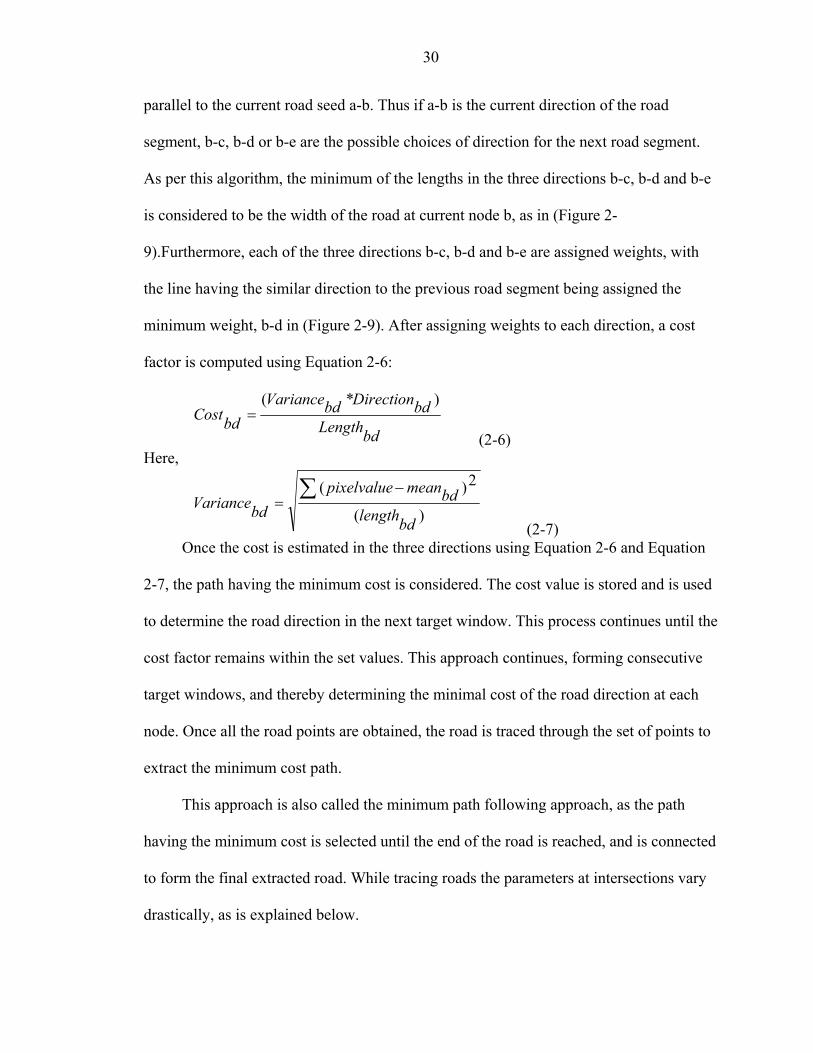
factor is computed using Equation 2-6:
bdLengthbdDirectionbdVariance
bdCost)*(
=
(2-6) Here,
)(
2)(
bdlengthbdmeanpixelvalue
bdVariance∑ −
=
(2-7) Once the cost is estimated in the three directions using Equation 2-6 and Equation
2-7, the path having the minimum cost is considered. The cost value is stored and is used
to determine the road direction in the next target window. This process continues until the
cost factor remains within the set values. This approach continues, forming consecutive
target windows, and thereby determining the minimal cost of the road direction at each
node. Once all the road points are obtained, the road is traced through the set of points to
extract the minimum cost path.
This approach is also called the minimum path following approach, as the path
having the minimum cost is selected until the end of the road is reached, and is connected
to form the final extracted road. While tracing roads the parameters at intersections vary
drastically, as is explained below.
31
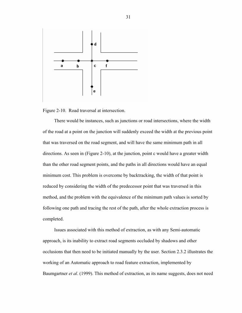
Figure 2-10. Road traversal at intersection.
There would be instances, such as junctions or road intersections, where the width
of the road at a point on the junction will suddenly exceed the width at the previous point
that was traversed on the road segment, and will have the same minimum path in all
directions. As seen in (Figure 2-10), at the junction, point c would have a greater width
than the other road segment points, and the paths in all directions would have an equal
minimum cost. This problem is overcome by backtracking, the width of that point is
reduced by considering the width of the predecessor point that was traversed in this
method, and the problem with the equivalence of the minimum path values is sorted by
following one path and tracing the rest of the path, after the whole extraction process is
completed.
Issues associated with this method of extraction, as with any Semi-automatic
approach, is its inability to extract road segments occluded by shadows and other
occlusions that then need to be initiated manually by the user. Section 2.3.2 illustrates the
working of an Automatic approach to road feature extraction, implemented by
Baumgartner et al. (1999). This method of extraction, as its name suggests, does not need
32
any initialization or feature identification step, these functions are performed by the
feature extraction method itself. This method of extraction includes some processes that
if implemented as stand-alone processes, would work as a Semi-automatic method of
extraction.
2.3.2 Multi-Scale and Snakes Road-Feature Extraction
The automatic method of extraction developed by Baumgartner et al. (1999),
explained in this section, gives an idea of the working of an Automatic method of
extraction, using information from various sources to extract road features from an aerial
image without any human intervention (Section 2.1).
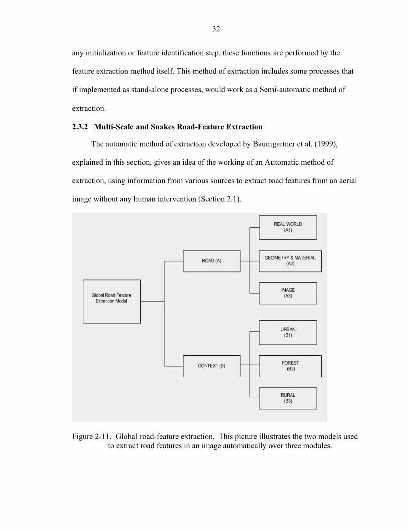
Figure 2-11. Global road-feature extraction. This picture illustrates the two models used
to extract road features in an image automatically over three modules.
33
Figure 2-11 illustrates an automatic method of extraction developed by
Baumgartner et al. (1999) to extract road features from aerial images using information
from coarse resolution and fine resolution images. The method of extraction is divided
into two models, a road model (A), and a contextual model (B), as shown in (Figure 2-
11).
The road model extracts the roads from an aerial image, from fine and coarse
resolutions of an input aerial image. At coarse resolution, the roads exist as splines or
long linear features, with intersections and junctions as blobs. At fine resolution, roads
exist as long homogenous regions with uniform radiometric variance. The road model
extracts roads at coarse resolution by assuming that road segments exist as long, bright
linear features. At fine resolution, the road model uses real world (A1) information (e.g.,
road pavement marking, geometry). It also uses material information (A2) determined
based on the width of the road segment and the overall radiometric variance of the road
segment, depending on the pavement type or material (e.g., asphalt and concrete), and
image characteristics of whether the identified road segment is an elongated bright
region. In brief, the road model introduced above extracts roads based on the road
segment’s geometric, radiometric, and topologic characteristics (Section 2.1).
The method of extraction developed by Baumgartner et al. (1999) also includes a
context model (B) in (Figure 2-11) that extracts road segments from the input image,
using information about other features that exist near the road segment. The context
model extracts the road from an input image using a global context and a local context.
These contexts support each other in the process of extraction. The global context (B)
sets an input image to an urban (B1), rural (B2), or forest (B3) as in (Figure 2-11). The
34
local context exists within the input image (e.g., a tree or building near a road segment),
that is occluded by the feature or its shadow, or individual road segments existing by
themselves. A tree occluding a road segment could occur whether the global context is
urban, rural or forest, whereas a building or its shadow occluding a road segment could
only occur in an urban or a rural area, where buildings such as residences or industrial
infrastructures may exist.
Thus, the global and local context within the context model work together to
extract road segments. This section explains the method of extraction in detail that uses
the road model and context model; it does so with the use of an example of rural (global
context) road feature extraction. Another significant point is that roads existing in an
urban area may not be able to be extracted in a similar fashion to those in a rural area,
since they may have different geometric and radiometric characteristics and contextual
information. Thus, the local context within an input image is assigned to a global context,
based on which roads are to be extracted. The model used depends on what information is
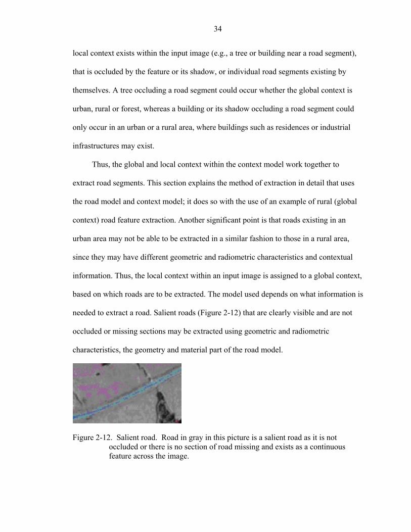
needed to extract a road. Salient roads (Figure 2-12) that are clearly visible and are not
occluded or missing sections may be extracted using geometric and radiometric
characteristics, the geometry and material part of the road model.
Figure 2-12. Salient road. Road in gray in this picture is a salient road as it is not
occluded or there is no section of road missing and exists as a continuous feature across the image.
35
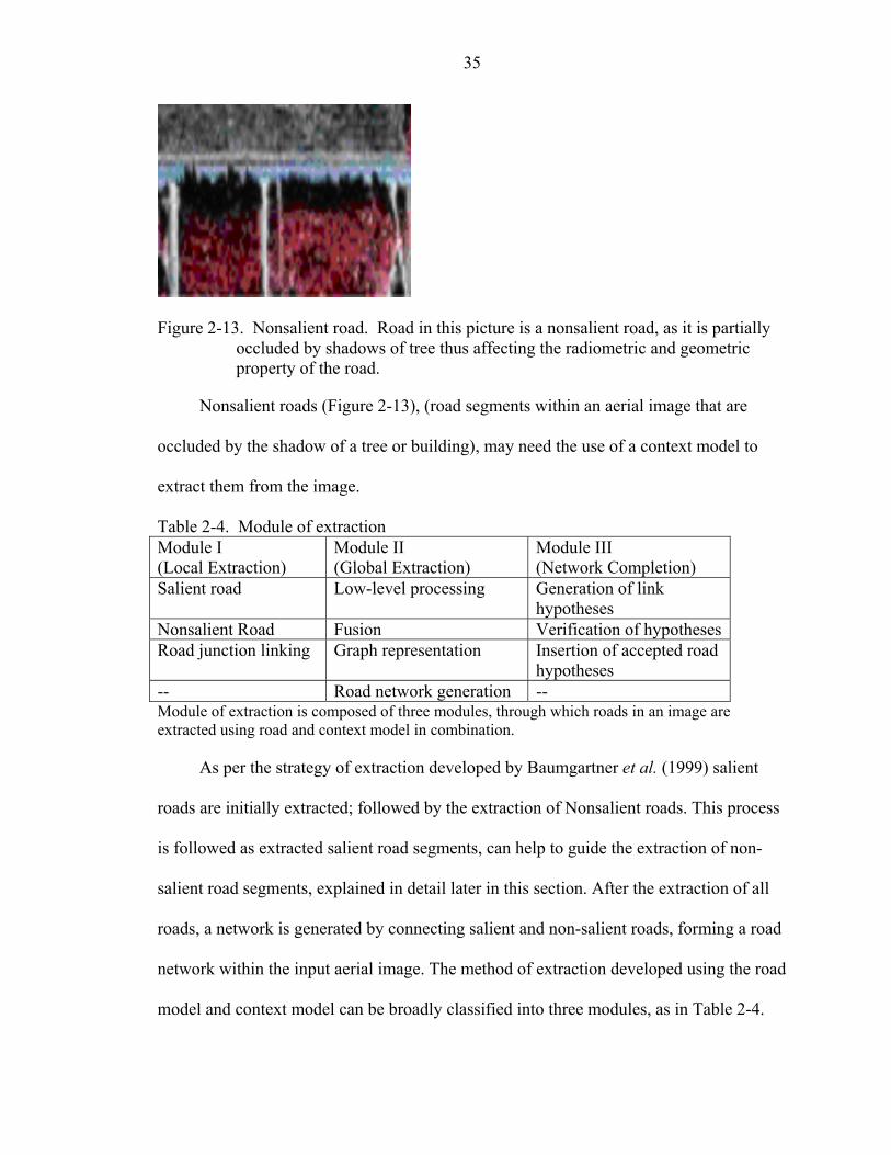
Figure 2-13. Nonsalient road. Road in this picture is a nonsalient road, as it is partially
occluded by shadows of tree thus affecting the radiometric and geometric property of the road.
Nonsalient roads (Figure 2-13), (road segments within an aerial image that are
occluded by the shadow of a tree or building), may need the use of a context model to
extract them from the image.
Table 2-4. Module of extraction Module I (Local Extraction)
Module II (Global Extraction)
Module III (Network Completion)
Salient road Low-level processing Generation of link hypotheses
Nonsalient Road Fusion Verification of hypothesesRoad junction linking Graph representation Insertion of accepted road
hypotheses -- Road network generation -- Module of extraction is composed of three modules, through which roads in an image are extracted using road and context model in combination.
As per the strategy of extraction developed by Baumgartner et al. (1999) salient
roads are initially extracted; followed by the extraction of Nonsalient roads. This process
is followed as extracted salient road segments, can help to guide the extraction of non-
salient road segments, explained in detail later in this section. After the extraction of all
roads, a network is generated by connecting salient and non-salient roads, forming a road
network within the input aerial image. The method of extraction developed using the road
model and context model can be broadly classified into three modules, as in Table 2-4.
36
Module I performs road extraction in a local context, using a high-resolution
image, initialized by extraction of salient road segments, followed by nonsalient road
segment extraction, and the extraction of the junctions or intersections that connect the
extracted road segments. Module II performs extraction in a global context, as a low level
processing step, using a low-resolution image as input. This is followed by the fusion of
the extracted road segments from the local level extraction that was implemented in
Module I, and the first step (low-level processing) implemented in Module II. The final
step of Module II involves the generation of a graph representing the road network from
the road segments generated from the fusion. Road segments obtained through this fusion
represent the edges, and its ends represent the set of vertices of the generated graph.
Module III of the developed method improves the extracted road network obtained
through Module I and II. It does so by the generation of link hypotheses, and their
verification, leading to the insertion of links. This allows complete extraction of the road
segments forming a network, without any broken road segment links. What follows in
this section explains in brief the implementation of each module.
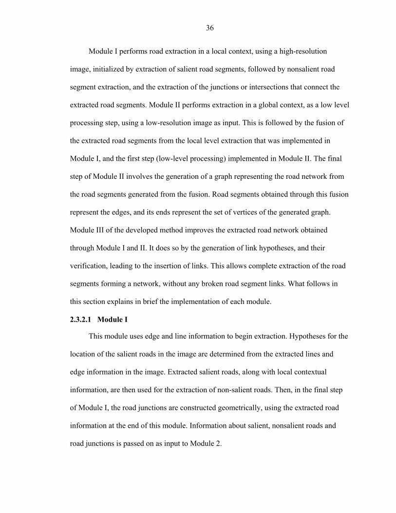
2.3.2.1 Module I
This module uses edge and line information to begin extraction. Hypotheses for the
location of the salient roads in the image are determined from the extracted lines and
edge information in the image. Extracted salient roads, along with local contextual
information, are then used for the extraction of non-salient roads. Then, in the final step
of Module I, the road junctions are constructed geometrically, using the extracted road
information at the end of this module. Information about salient, nonsalient roads and
road junctions is passed on as input to Module 2.
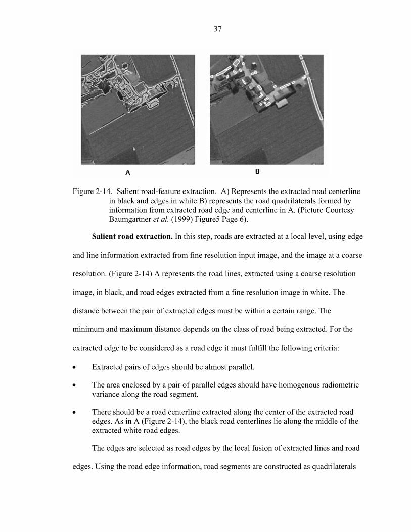
37
Figure 2-14. Salient road-feature extraction. A) Represents the extracted road centerline
in black and edges in white B) represents the road quadrilaterals formed by information from extracted road edge and centerline in A. (Picture Courtesy Baumgartner et al. (1999) Figure5 Page 6).
Salient road extraction. In this step, roads are extracted at a local level, using edge
and line information extracted from fine resolution input image, and the image at a coarse
resolution. (Figure 2-14) A represents the road lines, extracted using a coarse resolution
image, in black, and road edges extracted from a fine resolution image in white. The
distance between the pair of extracted edges must be within a certain range. The
minimum and maximum distance depends on the class of road being extracted. For the
extracted edge to be considered as a road edge it must fulfill the following criteria:
• Extracted pairs of edges should be almost parallel.
• The area enclosed by a pair of parallel edges should have homogenous radiometric variance along the road segment.
• There should be a road centerline extracted along the center of the extracted road edges. As in A (Figure 2-14), the black road centerlines lie along the middle of the extracted white road edges.
The edges are selected as road edges by the local fusion of extracted lines and road
edges. Using the road edge information, road segments are constructed as quadrilaterals

38
(Figure 2-14) that are generated from the parallel road edges. Quadrilaterals sharing
points with neighboring quadrilaterals are connected. The points on their axis, along with
the road width, represent the geometry of the road segments. This road information is
used as semantic information for the extraction of non-salient parts of the road network in
the next step of Module I.
Nonsalient road extraction. Nonsalient road segments cannot be extracted as
salient road segment, since they are occluded by the presence of cultural (e.g., buildings)
or natural (e.g., trees) objects or their shadows. Thus to extract a non-salient road, there is
a need for additional knowledge compared to the information needed for the extraction of
salient roads. This step of Module I, extracts non-salient road segments by linking the
extracted salient roads obtained from the previous step, and assuming that the non-salient
road segments are gaps between salient road segments. In addition to the linking of non-
salient roads, incorrect hypotheses for salient road segments are eliminated at this step.
As most of the road segments extracted by the fusion of local edge and line information
in previous step are short, the linking of correct road segments and the elimination of
false road segments is achieved by grouping salient road segments into longer segments.
This process is performed using the following hypothesis and test paradigm that groups
short salient road segments, bridging the gaps as well as extracting the non-salient road
segments.
Hypotheses concerning which road segments should be bridged, are generated
based on the comparison of the geometric (width, collinearity and distance) and
radiometric properties (mean gray value, standard deviation) of the new segment and the
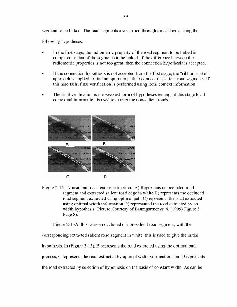
39
segment to be linked. The road segments are verified through three stages, using the
following hypotheses:
• In the first stage, the radiometric property of the road segment to be linked is compared to that of the segments to be linked. If the difference between the radiometric properties is not too great, then the connection hypothesis is accepted.
• If the connection hypothesis is not accepted from the first stage, the “ribbon snake” approach is applied to find an optimum path to connect the salient road segments. If this also fails, final verification is performed using local context information.
• The final verification is the weakest form of hypotheses testing, at this stage local contextual information is used to extract the non-salient roads.
Figure 2-15. Nonsalient road-feature extraction. A) Represents an occluded road
segment and extracted salient road edge in white B) represents the occluded road segment extracted using optimal path C) represents the road extracted using optimal width information D) represented the road extracted by on width hypothesis (Picture Courtesy of Baumgartner et al. (1999) Figure 8 Page 8).
Figure 2-15A illustrates an occluded or non-salient road segment, with the
corresponding extracted salient road segment in white; this is used to give the initial
hypothesis. In (Figure 2-15), B represents the road extracted using the optimal path
process, C represents the road extracted by optimal width verification, and D represents
the road extracted by selection of hypothesis on the basis of constant width. As can be
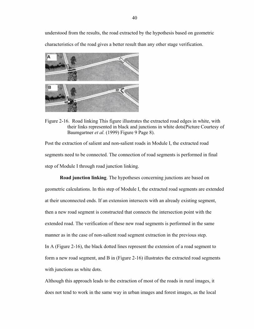
40
understood from the results, the road extracted by the hypothesis based on geometric
characteristics of the road gives a better result than any other stage verification.
Figure 2-16. Road linking This figure illustrates the extracted road edges in white, with
their links represented in black and junctions in white dots(Picture Courtesy of Baumgartner et al. (1999) Figure 9 Page 8).
Post the extraction of salient and non-salient roads in Module I, the extracted road
segments need to be connected. The connection of road segments is performed in final
step of Module I through road junction linking.
Road junction linking. The hypotheses concerning junctions are based on
geometric calculations. In this step of Module I, the extracted road segments are extended
at their unconnected ends. If an extension intersects with an already existing segment,
then a new road segment is constructed that connects the intersection point with the
extended road. The verification of these new road segments is performed in the same
manner as in the case of non-salient road segment extraction in the previous step.
In A (Figure 2-16), the black dotted lines represent the extension of a road segment to
form a new road segment, and B in (Figure 2-16) illustrates the extracted road segments
with junctions as white dots.
Although this approach leads to the extraction of most of the roads in rural images, it
does not tend to work in the same way in urban images and forest images, as the local

41
context for rural images is different to that in urban and forest images. In the case of
urban images, the network of roads may be denser, and their appearance may also be
different from the road segments existing in a rural image. The road features extracted in
this Module, i.e. Module I, were based on local context, i.e. within an image. Module I
extracted roads using geometric and radiometric properties of the road segment, and
concentrated on local criteria within an image to extract road edges. Module II performs
extraction on a global context, considering the whole image. In Module II, the topological
properties of the roads are used to extract roads, to support the extraction process
implemented in Module I, and improve upon the extracted results. The road network
extracted in Module II has more road segments than Module I as Module II is less
constrained.
2.3.2.2 Module II
An intrinsic topological characteristic of roads is to connect places. Roads are constructed
along paths that provide the shortest and most convenient way to reach places. This
property leads to searching for an optimal connection between places. The method of
determining the best connection between two points is of importance for road extraction.
This approach is feasible on low-resolution satellite images, as roads exist as linear bright
features, forming a network; they do not do so in high-resolution images, as high-
resolution images are more specific concerning individual road segments and their
geometric and radiometric properties. In this module, the approach adopted is modified to
integrate and process road like features from various input sources, i.e. lines extracted at
different scales. Module II performs extractions over four steps, i.e. Low-level
processing, Fusion, Graph Representation and Road Network generation. The
information obtained from Module I of the extraction process is passed on as input for
42
Module II. During the initial step of low-level processing, the roads that exist as long
bright features are extracted. These extracted features are further merged with road edges
extracted by local extraction in Module I, in the fusion step of Module II. The Graph
representation step constructs graphs using the fused road segments from the previous
step, with road segments represented by edges and the junctions of road segments as
vertices. The final step in Module II is to use the output of the Graph representation step
to generate the road network. The discussion below briefly explains each step.
Low-level processing. In this step, road segments are extracted by extracting a line
from a low-resolution image. This approach returns lines as sets of pixel chains, as well
as junction points, in sub-pixel precision. Some of the extracted lines may represent
actual roads, and some of the roads that are extracted may not necessarily be roads, they
may be other features such as rivers misidentified as roads. In the analysis of roads, the
behavior of several lines attributes is important, but the most significant change in lines is
high curvature. Hence, from the lines extracted at low-resolution, the lines were split into
road segments and non-road segments, based on points of high curvature, as the
probability of road having a very steep curve is low. If some road segments are
misidentified, or not identified at all, then they will be identified in the next step of the
fusion process. Here each extracted line feature that is classified as road segment is
supported by an extended description, based on the following calculated properties:
• Length
• Straightness, i.e. standard deviation of its direction.
• Width ( mean width of the extracted line).
• Constant Width ( standard deviation of the width).

43
• Constant radiometric value of a road segment (standard deviation of the intensity value along the segment).
Fusion. In this step, the road segments obtained from the previous step are
combined with the roads extracted from the local extraction performed in Module I. On
fusion, both types of road segments are stored as one set of linear data. Segments in this
linear data set are unified if they happen to lie within a buffer distance with a suitable
width, and if the two segments have a directional difference less than a set threshold,
otherwise they are evaluated as intersections. Overall, after the roads are extracted in this
Module, the result is a more complete network, than was extracted in Module I. However,
the process may also result in falsely detected road segments. Next, the extracted output
is represented in the form of a network graph.
Graph representation. Once the segments are fused, a graph is constructed, with
the road segments as edges and vertices as points of connectivity. In cases where two or
more segments intersect, only one point/vertex is retained, to preserve the topology of the
road. Attribute values of road segments, assigned in the low-level processing of this
Module, are used to weigh the graph, by associating every edge with a single weight. At
this step of the extraction it is difficult to determine whether a road junction between two
segments truly represents a connection of road segments. Thus, an additional hypothesis
is generated to determine the connections between the edges of the graph. The following
are the criteria that are used to measure the quality of the hypotheses:
Direction difference between adjacent road segments; either orthogonality (within road)
or orthogonality (at a T-junction) is assumed as a reference.
• The absolute length of the connection.
• The relative length of a connection compared to the length of the adjacent road segment with the lower weight.

44
• An additional constraint that prevents a connection hypothesis from assigning a higher weight than its adjacent road segments.
A linear fuzzy function is then defined to obtain fuzzy values for the hypothesis on each
of the above criteria; these values are then aggregated into an overall fuzzy value using
the fuzzy and operation. For example: a fuzzy function is defined for the difference in
direction to determine orthogonality within a road segment or at road segments. To prefer
either a continuation of the road segment, or to support the idea of a possible road
junction, a fuzzy function with two peaks is considered, one at o0 and one at
o90 , this
supports collinearity and junctions. Thus, a road connection may be classed as either a
road segment or a T-junction, by classing the connections as either a T-junction or a
collinear road segment. This classification can be built using the other parameters used
for evaluating junction hypotheses; for example the length of the connection as compared
to the length of the road segments to be connected, can be used as a weighting function in
the process of determining whether the connection is a junction or a road segment, by
using the above defined fuzzy value. Next the roads are generated using road seed
generation (points or places of interest to which a road connects) as the final step in
Module II.
Road network generation. Here, the road seeds are used in extracting roads, by
determining the optimal path between the seeds representing the origin and destination.
The seeds in this step are points of interest, like buildings, and industrial areas.
The algorithm for road network generation finds the shortest path using the Dijkstra-
Algorithm on the weight assigned to each road segment. Weights are assigned to road
segments depending on their fuzzy value. The weight (w) is assigned to a road segment
based on the fuzzy value that is assigned, these vary between 0 and 1, by using the true
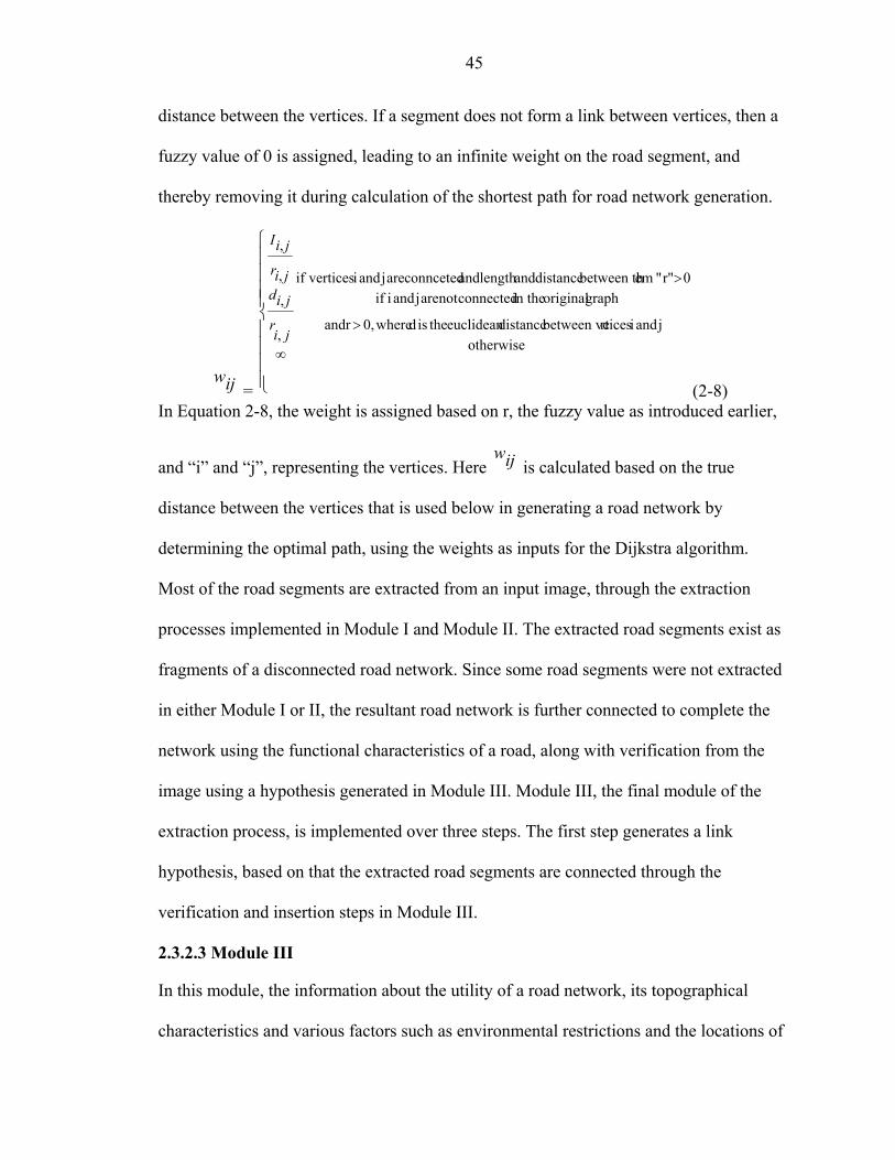
45
distance between the vertices. If a segment does not form a link between vertices, then a
fuzzy value of 0 is assigned, leading to an infinite weight on the road segment, and
thereby removing it during calculation of the shortest path for road network generation.
ijw =
otherwisej and i rticesbetween ve distanceeuclidean theis d where0,r and
graph original in the connectednot are j and i if 0 r" " embetween th distance andlength and connceted are j and i verticesif
,
,
,
,
>
>
∞
jir
jidjir
jiI
(2-8) In Equation 2-8, the weight is assigned based on r, the fuzzy value as introduced earlier,
and “i” and “j”, representing the vertices. Here ijw is calculated based on the true
distance between the vertices that is used below in generating a road network by
determining the optimal path, using the weights as inputs for the Dijkstra algorithm.
Most of the road segments are extracted from an input image, through the extraction
processes implemented in Module I and Module II. The extracted road segments exist as
fragments of a disconnected road network. Since some road segments were not extracted
in either Module I or II, the resultant road network is further connected to complete the
network using the functional characteristics of a road, along with verification from the
image using a hypothesis generated in Module III. Module III, the final module of the
extraction process, is implemented over three steps. The first step generates a link
hypothesis, based on that the extracted road segments are connected through the
verification and insertion steps in Module III.
2.3.2.3 Module III
In this module, the information about the utility of a road network, its topographical
characteristics and various factors such as environmental restrictions and the locations of
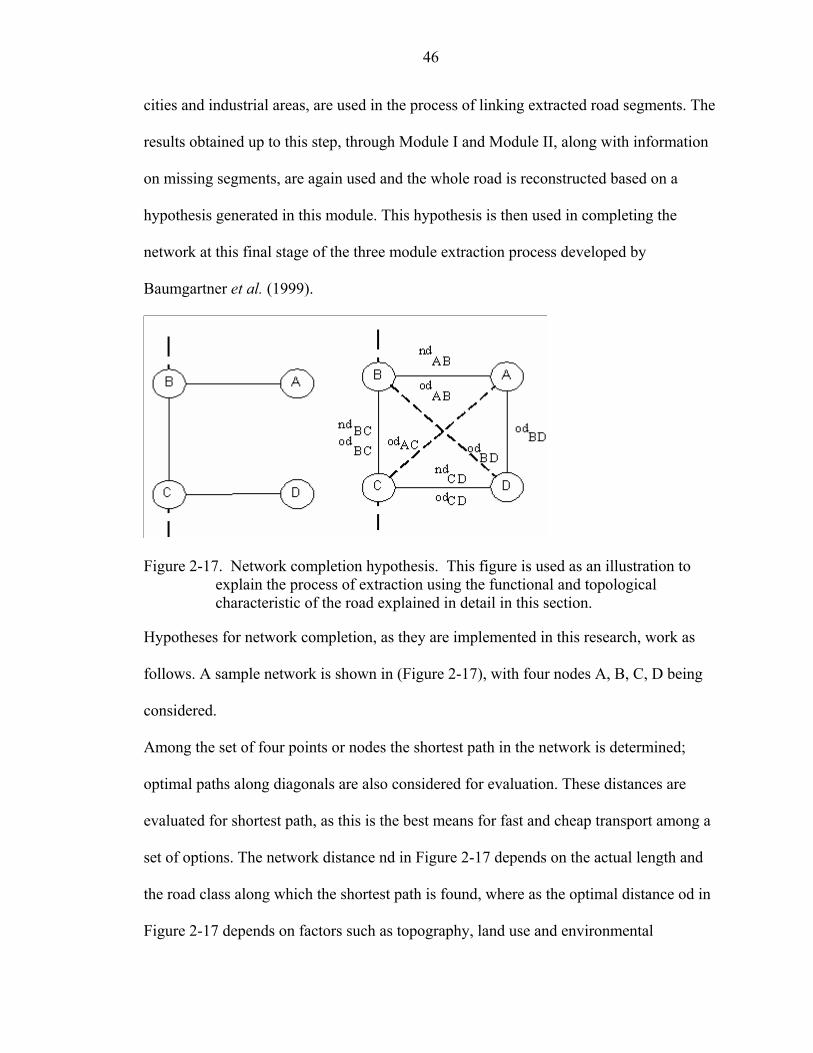
46
cities and industrial areas, are used in the process of linking extracted road segments. The
results obtained up to this step, through Module I and Module II, along with information
on missing segments, are again used and the whole road is reconstructed based on a
hypothesis generated in this module. This hypothesis is then used in completing the
network at this final stage of the three module extraction process developed by
Baumgartner et al. (1999).
Figure 2-17. Network completion hypothesis. This figure is used as an illustration to
explain the process of extraction using the functional and topological characteristic of the road explained in detail in this section.
Hypotheses for network completion, as they are implemented in this research, work as
follows. A sample network is shown in (Figure 2-17), with four nodes A, B, C, D being
considered.
Among the set of four points or nodes the shortest path in the network is determined;
optimal paths along diagonals are also considered for evaluation. These distances are
evaluated for shortest path, as this is the best means for fast and cheap transport among a
set of options. The network distance nd in Figure 2-17 depends on the actual length and
the road class along which the shortest path is found, where as the optimal distance od in
Figure 2-17 depends on factors such as topography, land use and environmental
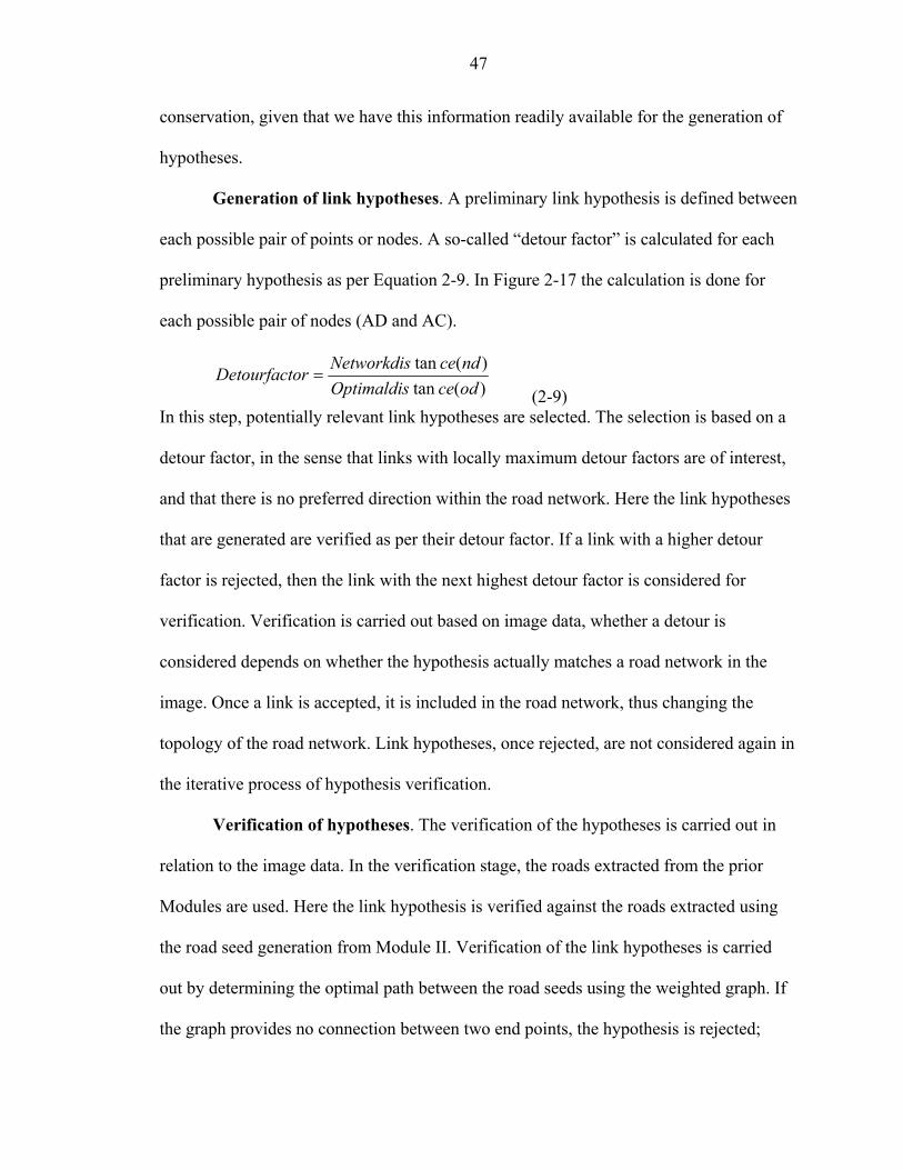
47
conservation, given that we have this information readily available for the generation of
hypotheses.
Generation of link hypotheses. A preliminary link hypothesis is defined between
each possible pair of points or nodes. A so-called “detour factor” is calculated for each
preliminary hypothesis as per Equation 2-9. In Figure 2-17 the calculation is done for
each possible pair of nodes (AD and AC).
)(tan)(tan
odceOptimaldisndceNetworkdis
orDetourfact = (2-9)
In this step, potentially relevant link hypotheses are selected. The selection is based on a
detour factor, in the sense that links with locally maximum detour factors are of interest,
and that there is no preferred direction within the road network. Here the link hypotheses
that are generated are verified as per their detour factor. If a link with a higher detour
factor is rejected, then the link with the next highest detour factor is considered for
verification. Verification is carried out based on image data, whether a detour is
considered depends on whether the hypothesis actually matches a road network in the
image. Once a link is accepted, it is included in the road network, thus changing the
topology of the road network. Link hypotheses, once rejected, are not considered again in
the iterative process of hypothesis verification.
Verification of hypotheses. The verification of the hypotheses is carried out in
relation to the image data. In the verification stage, the roads extracted from the prior
Modules are used. Here the link hypothesis is verified against the roads extracted using
the road seed generation from Module II. Verification of the link hypotheses is carried
out by determining the optimal path between the road seeds using the weighted graph. If
the graph provides no connection between two end points, the hypothesis is rejected;
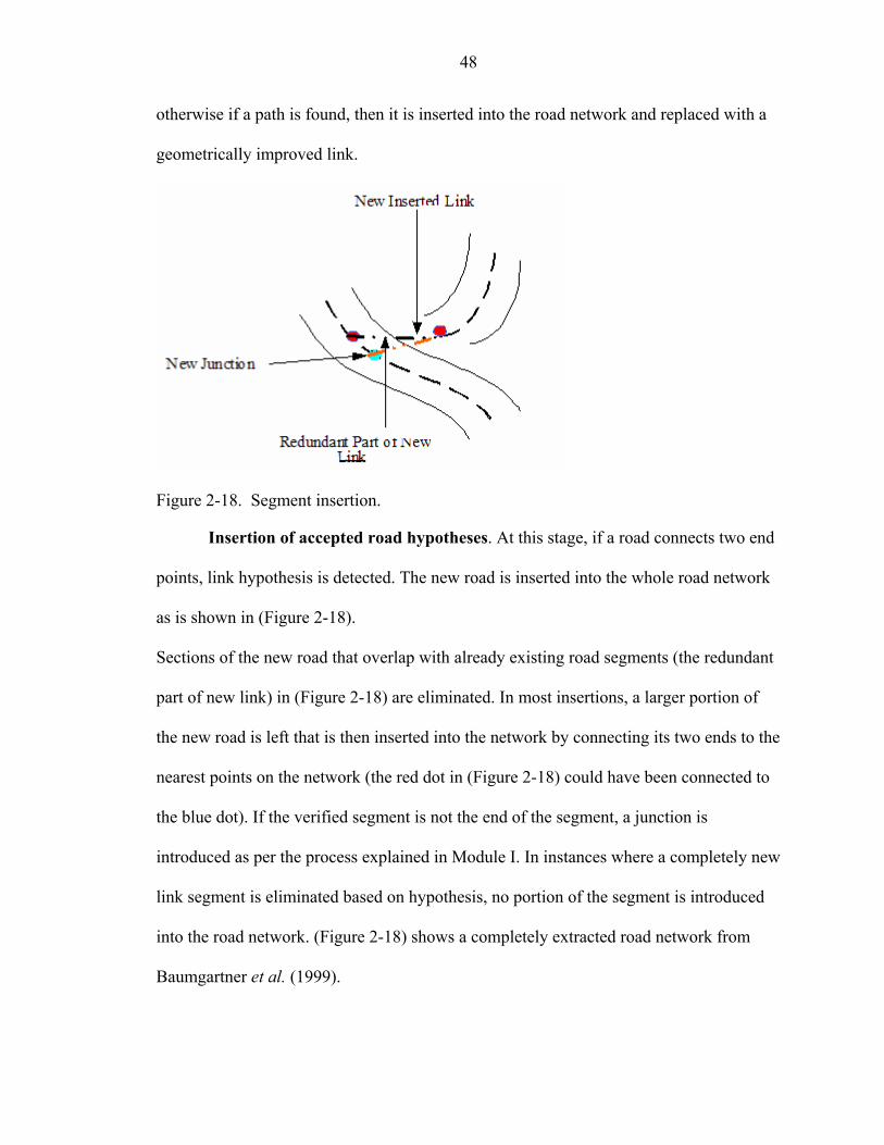
48
otherwise if a path is found, then it is inserted into the road network and replaced with a
geometrically improved link.
Figure 2-18. Segment insertion.
Insertion of accepted road hypotheses. At this stage, if a road connects two end
points, link hypothesis is detected. The new road is inserted into the whole road network
as is shown in (Figure 2-18).
Sections of the new road that overlap with already existing road segments (the redundant
part of new link) in (Figure 2-18) are eliminated. In most insertions, a larger portion of
the new road is left that is then inserted into the network by connecting its two ends to the
nearest points on the network (the red dot in (Figure 2-18) could have been connected to
the blue dot). If the verified segment is not the end of the segment, a junction is
introduced as per the process explained in Module I. In instances where a completely new
link segment is eliminated based on hypothesis, no portion of the segment is introduced
into the road network. (Figure 2-18) shows a completely extracted road network from
Baumgartner et al. (1999).
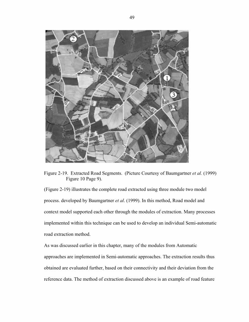
49
Figure 2-19. Extracted Road Segments. (Picture Courtesy of Baumgartner et al. (1999)
Figure 10 Page 9).
(Figure 2-19) illustrates the complete road extracted using three module two model
process. developed by Baumgartner et al. (1999). In this method, Road model and
context model supported each other through the modules of extraction. Many processes
implemented within this technique can be used to develop an individual Semi-automatic
road extraction method.
As was discussed earlier in this chapter, many of the modules from Automatic
approaches are implemented in Semi-automatic approaches. The extraction results thus
obtained are evaluated further, based on their connectivity and their deviation from the
reference data. The method of extraction discussed above is an example of road feature

50
extraction for a rural road. In case of urban road extraction, information from sources as
Digital surface models, along with contextual information. are needed to make the
approach automatic.
This chapter was an overview of the various characteristics that affect the road extraction
process, and different approaches to road extraction. Chapters 3 and 4 introduce the
Perona-Malik algorithm and Snakes Theory. In our study a Semi-automatic road feature
extraction method is developed, using anisotropic diffusion, rather than Gaussian blurring
(isotropic diffusion) that is implemented through the Perona–Malik algorithm (explained
in Chapter 3). In Chapter 4, the theory and concept of Snakes, and its implementation for
feature extraction, is explained; it will be implemented in our study to extract road
features from diffused image information using dynamic Snakes. The method of road
feature extraction is explained in Chapter 5 that uses the anisotropic diffusion approach
developed by Perona and Malik and Snakes to extract roads. Chapter 6 discusses the
results obtained, followed by an evaluation and analysis of the results. Chapter 7
concludes the thesis with an overview of the method of extraction implemented in our
study, and the future work to be pursued in this research. The automation of the initial
step of feature identification and the selection of road segments is one of the essential
pieces of work to be carried out in the future. Automation of initial identification, using
the Kalman Filter and Profile matching, is explained, as a possibility for the initial road
identification step, prior to the feature extraction method implementation (Appendix B).
51
CHAPTER 3 ANISOTROPIC DIFFUSION AND THE PERONA–MALIK ALGORITHM
An image is in general a photometric representation of real world features. Objects
or features from the real world are represented as regions composed of a group of pixels,
typically with similar intensity values, in a digital image. Features or objects represented
in an image may have similar pixel intensity values, at least within each feature or object
existing as a region in an image. Ideally such features may be represented as homogenous
regions within an image, for example buildings, trees, or agricultural land within a high-
resolution image, may be represented as regions with similar pixel intensity values
overall. During the capture and development of this information into a digital image,
noise or undesired information is also generated, affecting the representation of the real-
world features in the image. The noise exists as blobs on the image, with pixel intensity
values different from the overall or average pixel intensity values that represent a
particular region or feature.
Many fields use information extracted from an image for varied purposes: medical
image analysis etc. During the process of extraction, the existence of noise leads to
misrepresentation or false feature extraction. A feature extraction method usually extracts
the desired features from an image based on shape and feature boundary descriptions,
obtained through the edge detection step of the feature extraction method. The existence
of noise within an image affects the feature extraction step, as noise results in false edges
being detected that may not exist in the real world and should not exist in the
representation of the feature in the image.
52
To overcome this problem, noise across the image is minimized by implementing
blurring or smoothing operations; this is done at the initial step of pre-processing in the
feature extraction method. In general, smoothing operations assign each pixel within the
input image a new intensity value that is calculated from the intensity of the pixel values
in its neighborhood in the digital image. This process thereby minimizes variation across
pixels, and consequently reduces the noise within an image. The resultant image is a
blurred or smoothed variant of the original input image. The image obtained from the
pre-processing step is thus significant in extraction of desired features. Below, Section
3.1 explains the principles of isotropic and anisotropic diffusion; this is followed by a
discussion on the need and implementation of anisotropic diffusion in the Perona-Malik
algorithm in Section 3.2. Section 3.2.1 explains the process of intra region blurring,
carried out using the Perona-Malik algorithm, while simultaneously performing Local
edge enhancement, as is explained in Section 3.2.2. This chapter concludes with an
illustration of the algorithm’s implementation on an image lattice structure (Malik and
Perona, 1990).
3.1 Principles of Isotropic and Anisotropic Diffusion
Conventional smoothing operations implemented at the pre-processing step are
usually performed using a Gaussian, Laplacian etc. system. Blurring performed using a
Gaussian system blurs the image by assigning each pixel a value based on the weighted
average of the local pixel intensity values that are calculated using a Gaussian
distribution kernel (Section 2.2.1). Conventional smoothing techniques perform well
when used to minimize variation across the image. The process of blurring performed by
a conventional technique, like Gaussian, is isotropic in nature; conventional technique
will blur the whole image in a similar fashion in all directions. This isotropic property of
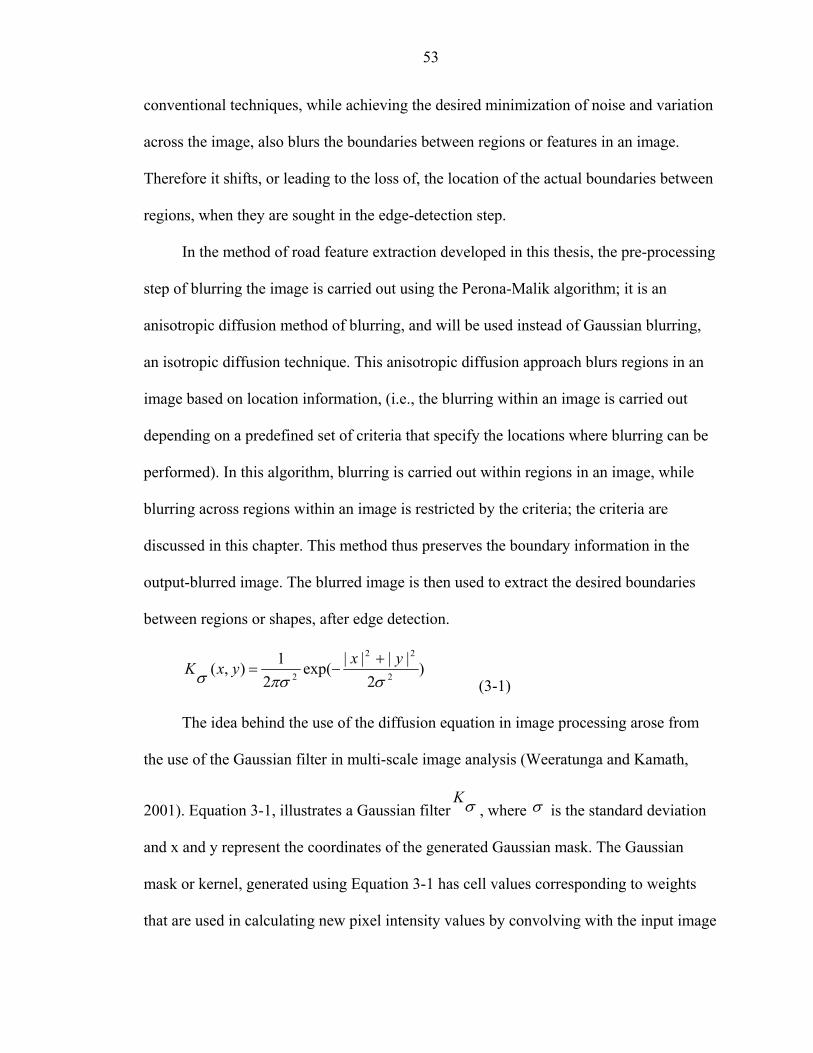
53
conventional techniques, while achieving the desired minimization of noise and variation
across the image, also blurs the boundaries between regions or features in an image.
Therefore it shifts, or leading to the loss of, the location of the actual boundaries between
regions, when they are sought in the edge-detection step.
In the method of road feature extraction developed in this thesis, the pre-processing
step of blurring the image is carried out using the Perona-Malik algorithm; it is an
anisotropic diffusion method of blurring, and will be used instead of Gaussian blurring,
an isotropic diffusion technique. This anisotropic diffusion approach blurs regions in an
image based on location information, (i.e., the blurring within an image is carried out
depending on a predefined set of criteria that specify the locations where blurring can be
performed). In this algorithm, blurring is carried out within regions in an image, while
blurring across regions within an image is restricted by the criteria; the criteria are
discussed in this chapter. This method thus preserves the boundary information in the
output-blurred image. The blurred image is then used to extract the desired boundaries
between regions or shapes, after edge detection.
)2
||||exp(2
1),( 2
22
2 σπσσyxyxK +
−= (3-1)
The idea behind the use of the diffusion equation in image processing arose from
the use of the Gaussian filter in multi-scale image analysis (Weeratunga and Kamath,
2001). Equation 3-1, illustrates a Gaussian filter σK, where σ is the standard deviation
and x and y represent the coordinates of the generated Gaussian mask. The Gaussian
mask or kernel, generated using Equation 3-1 has cell values corresponding to weights
that are used in calculating new pixel intensity values by convolving with the input image
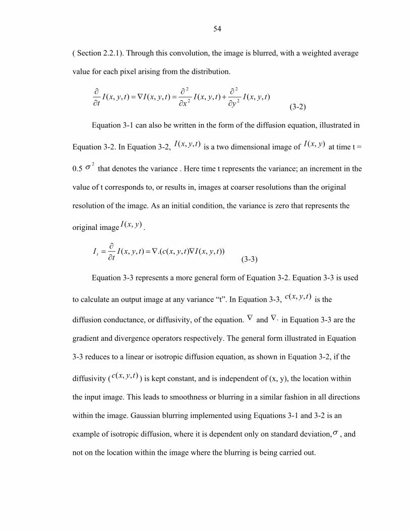
54
( Section 2.2.1). Through this convolution, the image is blurred, with a weighted average
value for each pixel arising from the distribution.
),,(),,(),,(),,(2
2
2
2
tyxIy
tyxIx
tyxItyxIt ∂
∂+
∂∂
=∇=∂∂
(3-2)
Equation 3-1 can also be written in the form of the diffusion equation, illustrated in
Equation 3-2. In Equation 3-2, ),,( tyxI is a two dimensional image of ),( yxI at time t =
0.5 2σ that denotes the variance . Here time t represents the variance; an increment in the
value of t corresponds to, or results in, images at coarser resolutions than the original
resolution of the image. As an initial condition, the variance is zero that represents the
original image ),( yxI .
)),,(),,(.(),,( tyxItyxctyxIt
I t ∇∇=∂∂
= (3-3)
Equation 3-3 represents a more general form of Equation 3-2. Equation 3-3 is used
to calculate an output image at any variance “t”. In Equation 3-3, ),,( tyxc is the
diffusion conductance, or diffusivity, of the equation. ∇ and .∇ in Equation 3-3 are the
gradient and divergence operators respectively. The general form illustrated in Equation
3-3 reduces to a linear or isotropic diffusion equation, as shown in Equation 3-2, if the
diffusivity ( ),,( tyxc ) is kept constant, and is independent of (x, y), the location within
the input image. This leads to smoothness or blurring in a similar fashion in all directions
within the image. Gaussian blurring implemented using Equations 3-1 and 3-2 is an
example of isotropic diffusion, where it is dependent only on standard deviation,σ , and
not on the location within the image where the blurring is being carried out.
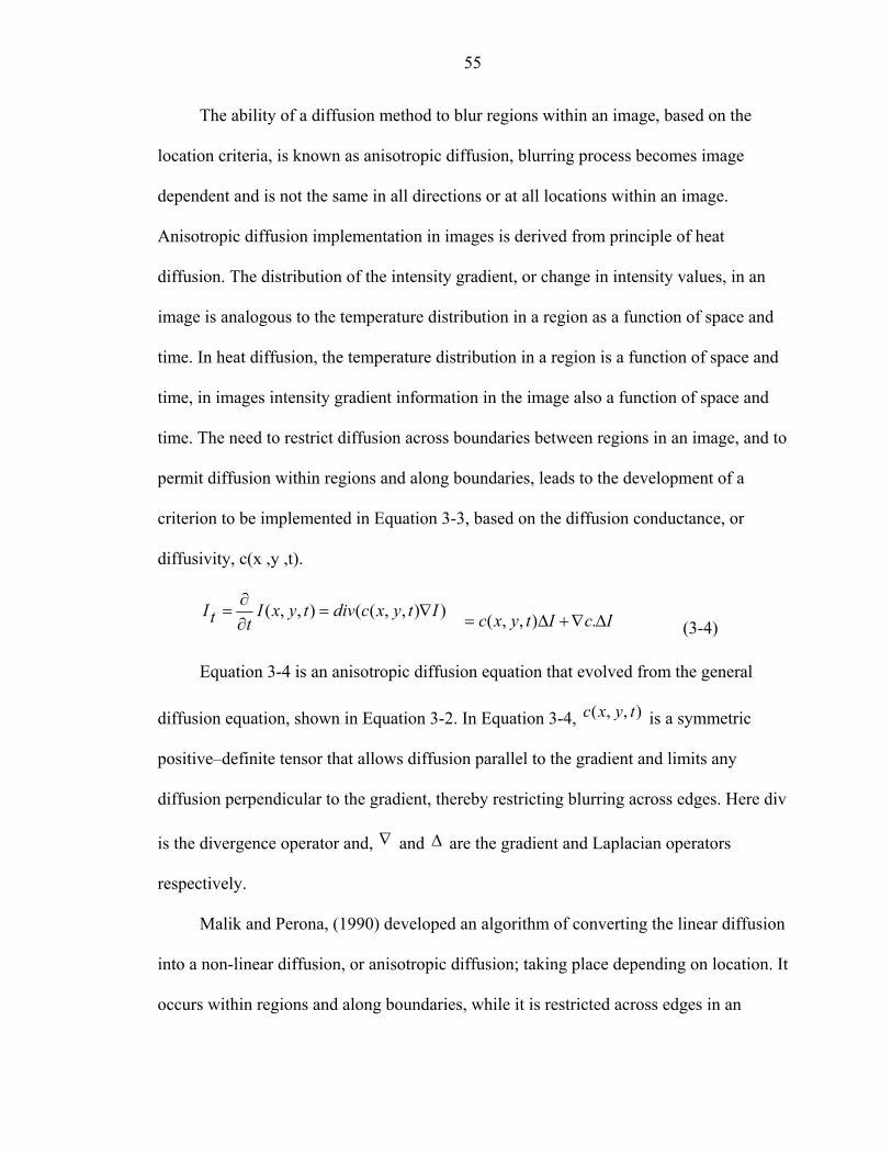
55
The ability of a diffusion method to blur regions within an image, based on the
location criteria, is known as anisotropic diffusion, blurring process becomes image
dependent and is not the same in all directions or at all locations within an image.
Anisotropic diffusion implementation in images is derived from principle of heat
diffusion. The distribution of the intensity gradient, or change in intensity values, in an
image is analogous to the temperature distribution in a region as a function of space and
time. In heat diffusion, the temperature distribution in a region is a function of space and
time, in images intensity gradient information in the image also a function of space and
time. The need to restrict diffusion across boundaries between regions in an image, and to
permit diffusion within regions and along boundaries, leads to the development of a
criterion to be implemented in Equation 3-3, based on the diffusion conductance, or
diffusivity, c(x ,y ,t).
)),,((),,( ItyxcdivtyxIttI ∇=∂∂
= IcItyxc ∆∇+∆= .),,( (3-4)
Equation 3-4 is an anisotropic diffusion equation that evolved from the general
diffusion equation, shown in Equation 3-2. In Equation 3-4, ),,( tyxc is a symmetric
positive–definite tensor that allows diffusion parallel to the gradient and limits any
diffusion perpendicular to the gradient, thereby restricting blurring across edges. Here div
is the divergence operator and, ∇ and ∆ are the gradient and Laplacian operators
respectively.
Malik and Perona, (1990) developed an algorithm of converting the linear diffusion
into a non-linear diffusion, or anisotropic diffusion; taking place depending on location. It
occurs within regions and along boundaries, while it is restricted across edges in an
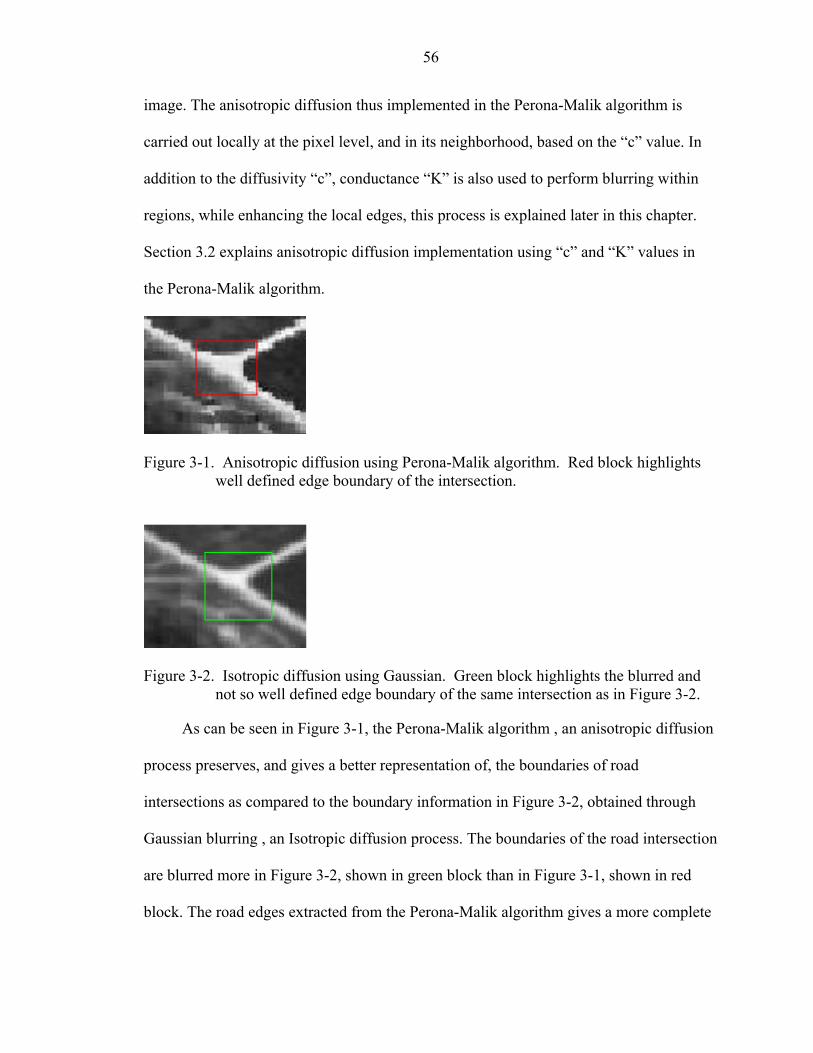
56
image. The anisotropic diffusion thus implemented in the Perona-Malik algorithm is
carried out locally at the pixel level, and in its neighborhood, based on the “c” value. In
addition to the diffusivity “c”, conductance “K” is also used to perform blurring within
regions, while enhancing the local edges, this process is explained later in this chapter.
Section 3.2 explains anisotropic diffusion implementation using “c” and “K” values in
the Perona-Malik algorithm.
Figure 3-1. Anisotropic diffusion using Perona-Malik algorithm. Red block highlights
well defined edge boundary of the intersection.
Figure 3-2. Isotropic diffusion using Gaussian. Green block highlights the blurred and
not so well defined edge boundary of the same intersection as in Figure 3-2.
As can be seen in Figure 3-1, the Perona-Malik algorithm , an anisotropic diffusion
process preserves, and gives a better representation of, the boundaries of road
intersections as compared to the boundary information in Figure 3-2, obtained through
Gaussian blurring , an Isotropic diffusion process. The boundaries of the road intersection
are blurred more in Figure 3-2, shown in green block than in Figure 3-1, shown in red
block. The road edges extracted from the Perona-Malik algorithm gives a more complete
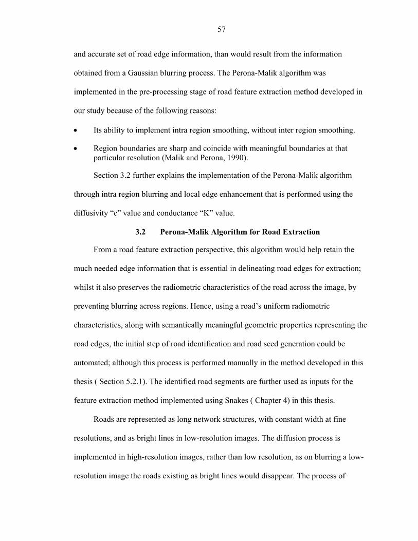
57
and accurate set of road edge information, than would result from the information
obtained from a Gaussian blurring process. The Perona-Malik algorithm was
implemented in the pre-processing stage of road feature extraction method developed in
our study because of the following reasons:
• Its ability to implement intra region smoothing, without inter region smoothing.
• Region boundaries are sharp and coincide with meaningful boundaries at that particular resolution (Malik and Perona, 1990).
Section 3.2 further explains the implementation of the Perona-Malik algorithm
through intra region blurring and local edge enhancement that is performed using the
diffusivity “c” value and conductance “K” value.
3.2 Perona-Malik Algorithm for Road Extraction
From a road feature extraction perspective, this algorithm would help retain the
much needed edge information that is essential in delineating road edges for extraction;
whilst it also preserves the radiometric characteristics of the road across the image, by
preventing blurring across regions. Hence, using a road’s uniform radiometric
characteristics, along with semantically meaningful geometric properties representing the
road edges, the initial step of road identification and road seed generation could be
automated; although this process is performed manually in the method developed in this
thesis ( Section 5.2.1). The identified road segments are further used as inputs for the
feature extraction method implemented using Snakes ( Chapter 4) in this thesis.
Roads are represented as long network structures, with constant width at fine
resolutions, and as bright lines in low-resolution images. The diffusion process is
implemented in high-resolution images, rather than low resolution, as on blurring a low-
resolution image the roads existing as bright lines would disappear. The process of
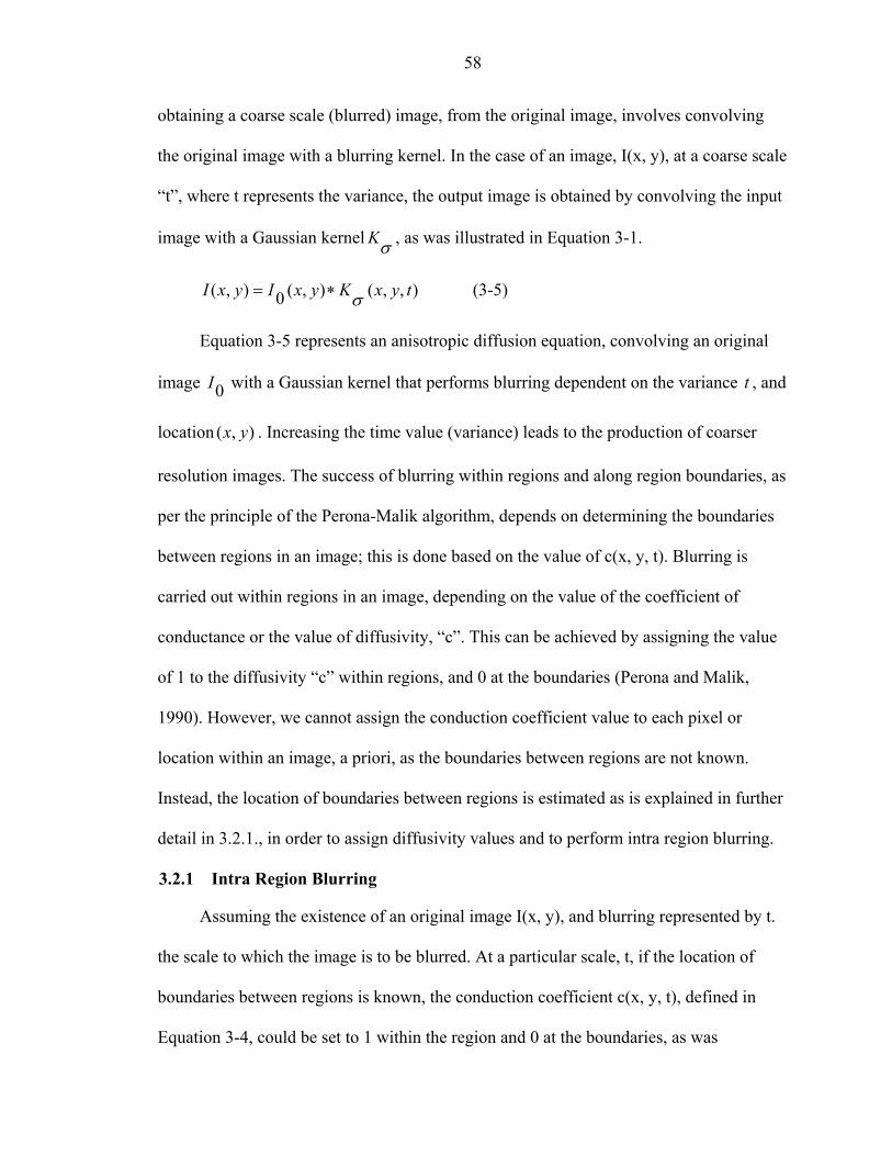
58
obtaining a coarse scale (blurred) image, from the original image, involves convolving
the original image with a blurring kernel. In the case of an image, I(x, y), at a coarse scale
“t”, where t represents the variance, the output image is obtained by convolving the input
image with a Gaussian kernel σK , as was illustrated in Equation 3-1.
),,(),(0),( tyxKyxIyxI σ∗= (3-5)
Equation 3-5 represents an anisotropic diffusion equation, convolving an original
image 0I with a Gaussian kernel that performs blurring dependent on the variance t , and
location ),( yx . Increasing the time value (variance) leads to the production of coarser
resolution images. The success of blurring within regions and along region boundaries, as
per the principle of the Perona-Malik algorithm, depends on determining the boundaries
between regions in an image; this is done based on the value of c(x, y, t). Blurring is
carried out within regions in an image, depending on the value of the coefficient of
conductance or the value of diffusivity, “c”. This can be achieved by assigning the value
of 1 to the diffusivity “c” within regions, and 0 at the boundaries (Perona and Malik,
1990). However, we cannot assign the conduction coefficient value to each pixel or
location within an image, a priori, as the boundaries between regions are not known.
Instead, the location of boundaries between regions is estimated as is explained in further
detail in 3.2.1., in order to assign diffusivity values and to perform intra region blurring.
3.2.1 Intra Region Blurring
Assuming the existence of an original image I(x, y), and blurring represented by t.
the scale to which the image is to be blurred. At a particular scale, t, if the location of
boundaries between regions is known, the conduction coefficient c(x, y, t), defined in
Equation 3-4, could be set to 1 within the region and 0 at the boundaries, as was
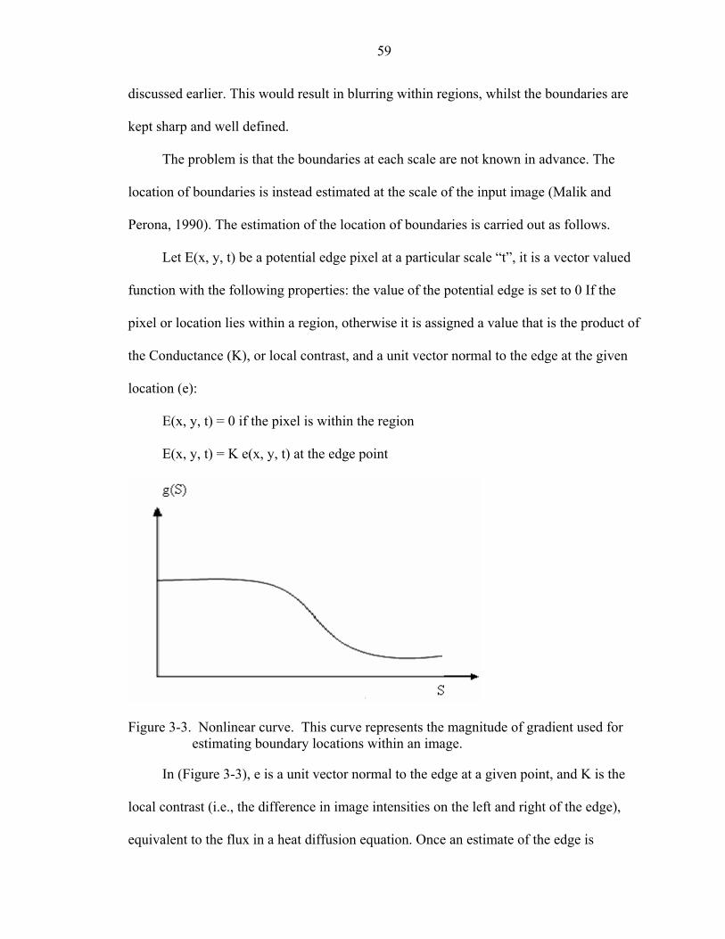
59
discussed earlier. This would result in blurring within regions, whilst the boundaries are
kept sharp and well defined.
The problem is that the boundaries at each scale are not known in advance. The
location of boundaries is instead estimated at the scale of the input image (Malik and
Perona, 1990). The estimation of the location of boundaries is carried out as follows.
Let E(x, y, t) be a potential edge pixel at a particular scale “t”, it is a vector valued
function with the following properties: the value of the potential edge is set to 0 If the
pixel or location lies within a region, otherwise it is assigned a value that is the product of
the Conductance (K), or local contrast, and a unit vector normal to the edge at the given
location (e):
E(x, y, t) = 0 if the pixel is within the region
E(x, y, t) = K e(x, y, t) at the edge point
Figure 3-3. Nonlinear curve. This curve represents the magnitude of gradient used for
estimating boundary locations within an image.
In (Figure 3-3), e is a unit vector normal to the edge at a given point, and K is the
local contrast (i.e., the difference in image intensities on the left and right of the edge),
equivalent to the flux in a heat diffusion equation. Once an estimate of the edge is
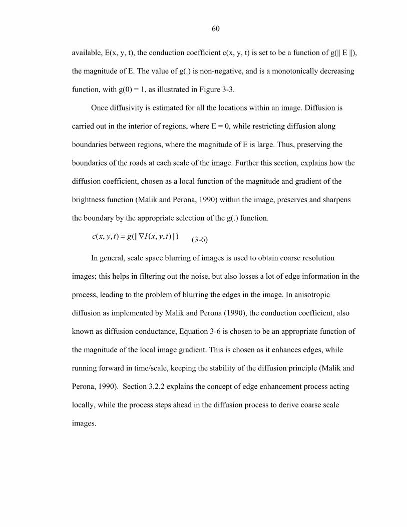
60
available, E(x, y, t), the conduction coefficient c(x, y, t) is set to be a function of g(|| E ||),
the magnitude of E. The value of g(.) is non-negative, and is a monotonically decreasing
function, with g(0) = 1, as illustrated in Figure 3-3.
Once diffusivity is estimated for all the locations within an image. Diffusion is
carried out in the interior of regions, where E = 0, while restricting diffusion along
boundaries between regions, where the magnitude of E is large. Thus, preserving the
boundaries of the roads at each scale of the image. Further this section, explains how the
diffusion coefficient, chosen as a local function of the magnitude and gradient of the
brightness function (Malik and Perona, 1990) within the image, preserves and sharpens
the boundary by the appropriate selection of the g(.) function.
||)),,((||),,( tyxIgtyxc ∇= (3-6)
In general, scale space blurring of images is used to obtain coarse resolution
images; this helps in filtering out the noise, but also losses a lot of edge information in the
process, leading to the problem of blurring the edges in the image. In anisotropic
diffusion as implemented by Malik and Perona (1990), the conduction coefficient, also
known as diffusion conductance, Equation 3-6 is chosen to be an appropriate function of
the magnitude of the local image gradient. This is chosen as it enhances edges, while
running forward in time/scale, keeping the stability of the diffusion principle (Malik and
Perona, 1990). Section 3.2.2 explains the concept of edge enhancement process acting
locally, while the process steps ahead in the diffusion process to derive coarse scale
images.
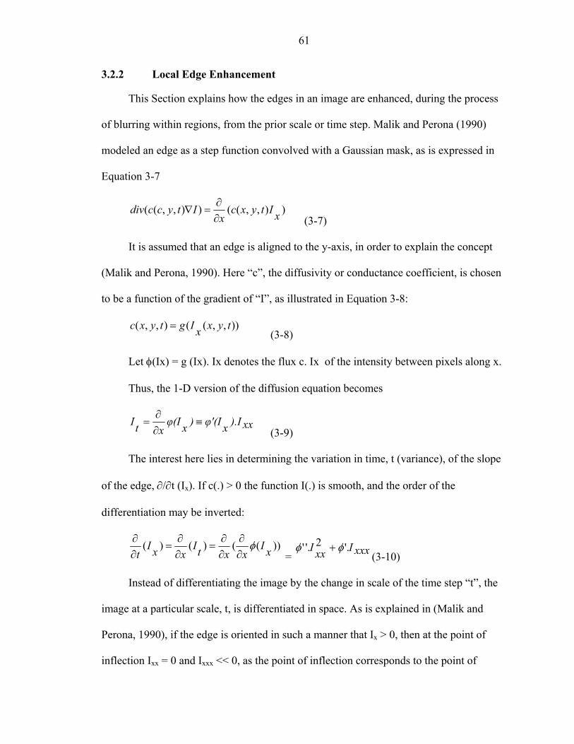
61
3.2.2 Local Edge Enhancement
This Section explains how the edges in an image are enhanced, during the process
of blurring within regions, from the prior scale or time step. Malik and Perona (1990)
modeled an edge as a step function convolved with a Gaussian mask, as is expressed in
Equation 3-7
)),,(()),,(( xItyxcx
Ityccdiv∂∂
=∇ (3-7)
It is assumed that an edge is aligned to the y-axis, in order to explain the concept
(Malik and Perona, 1990). Here “c”, the diffusivity or conductance coefficient, is chosen
to be a function of the gradient of “I”, as illustrated in Equation 3-8:
)),,((),,( tyxxIgtyxc = (3-8)
Let φ(Ix) = g (Ix). Ix denotes the flux c. Ix of the intensity between pixels along x.
Thus, the 1-D version of the diffusion equation becomes
xx).Ixφ'(I)xφ(IxtI ≡∂∂
= (3-9)
The interest here lies in determining the variation in time, t (variance), of the slope
of the edge, ∂/∂t (Ix). If c(.) > 0 the function I(.) is smooth, and the order of the
differentiation may be inverted:
))(()()( xIxxtI
xxIt
φ∂∂
∂∂
=∂∂
=∂∂
= xxxIxxI '.2'.' φφ + (3-10)
Instead of differentiating the image by the change in scale of the time step “t”, the
image at a particular scale, t, is differentiated in space. As is explained in (Malik and
Perona, 1990), if the edge is oriented in such a manner that Ix > 0, then at the point of
inflection Ixx = 0 and Ixxx << 0, as the point of inflection corresponds to the point of
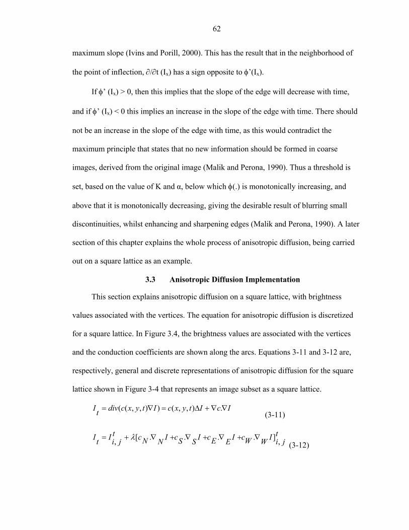
62
maximum slope (Ivins and Porill, 2000). This has the result that in the neighborhood of
the point of inflection, ∂/∂t (Ix) has a sign opposite to φ’(Ix).
If φ’ (Ix) > 0, then this implies that the slope of the edge will decrease with time,
and if φ’ (Ix) < 0 this implies an increase in the slope of the edge with time. There should
not be an increase in the slope of the edge with time, as this would contradict the
maximum principle that states that no new information should be formed in coarse
images, derived from the original image (Malik and Perona, 1990). Thus a threshold is
set, based on the value of K and α, below which φ(.) is monotonically increasing, and
above that it is monotonically decreasing, giving the desirable result of blurring small
discontinuities, whilst enhancing and sharpening edges (Malik and Perona, 1990). A later
section of this chapter explains the whole process of anisotropic diffusion, being carried
out on a square lattice as an example.
3.3 Anisotropic Diffusion Implementation
This section explains anisotropic diffusion on a square lattice, with brightness
values associated with the vertices. The equation for anisotropic diffusion is discretized
for a square lattice. In Figure 3.4, the brightness values are associated with the vertices
and the conduction coefficients are shown along the arcs. Equations 3-11 and 3-12 are,
respectively, general and discrete representations of anisotropic diffusion for the square
lattice shown in Figure 3-4 that represents an image subset as a square lattice.
IcItyxcItyxcdivtI ∇∇+∆=∇= .),,()),,(( (3-11)
tjiIWWcIEEcISScINNct
jiItI ,]....[, ∇+∇+∇+∇+= λ (3-12)
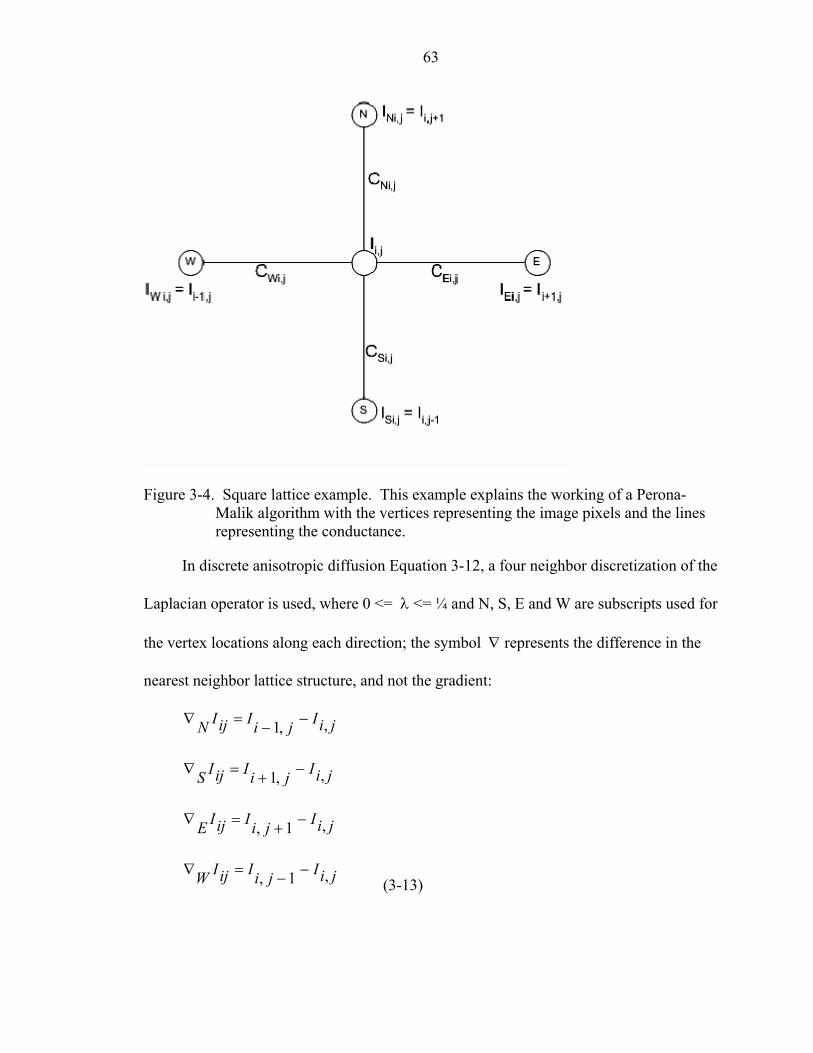
63
Figure 3-4. Square lattice example. This example explains the working of a Perona-Malik algorithm with the vertices representing the image pixels and the lines representing the conductance.
In discrete anisotropic diffusion Equation 3-12, a four neighbor discretization of the
Laplacian operator is used, where 0 <= λ <= ¼ and N, S, E and W are subscripts used for
the vertex locations along each direction; the symbol ∇ represents the difference in the
nearest neighbor lattice structure, and not the gradient:
jiIjiIijIN ,,1 −−=∇
jiIjiIijIS ,,1 −+=∇
jiIjiIijIE ,1, −+=∇
jiIjiIijIW ,1, −−=∇ (3-13)
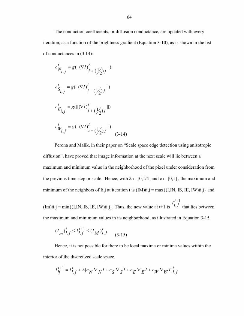
64
The conduction coefficients, or diffusion conductance, are updated with every
iteration, as a function of the brightness gradient (Equation 3-10), as is shown in the list
of conductances in (3.14):
||))2
1()((||
,t
jiIgt
jiNc+
∇=
||))2
1()((||
,t
jiIgt
jiSc−
∇=
||))2
1()((||
,t
jiIgt
jiEc+
∇=
||))2
1()((||
,t
jiIgt
jiWc−
∇=
(3-14)
Perona and Malik, in their paper on “Scale space edge detection using anisotropic
diffusion”, have proved that image information at the next scale will lie between a
maximum and minimum value in the neighborhood of the pixel under consideration from
the previous time step or scale. Hence, with λ ∈ [0,1/4] and c ∈ [0,1] , the maximum and
minimum of the neighbors of Ii,j at iteration t is (IM)ti,j = max{(I,IN, IS, IE, IW)ti,j} and
(Im)ti,j = min{(I,IN, IS, IE, IW)ti,j}. Thus, the new value at t+1 is 1
,+tjiI
that lies between
the maximum and minimum values in its neighborhood, as illustrated in Equation 3-15.
tjiMIt
jiItjimI ,)(1
,,)( ≤+≤ (3-15)
Hence, it is not possible for there to be local maxima or minima values within the
interior of the discretized scale space.
tjiIWWcIEEcISScINNct
jiItijI ,]....[,
1 ∇+∇+∇+∇+=+ λ
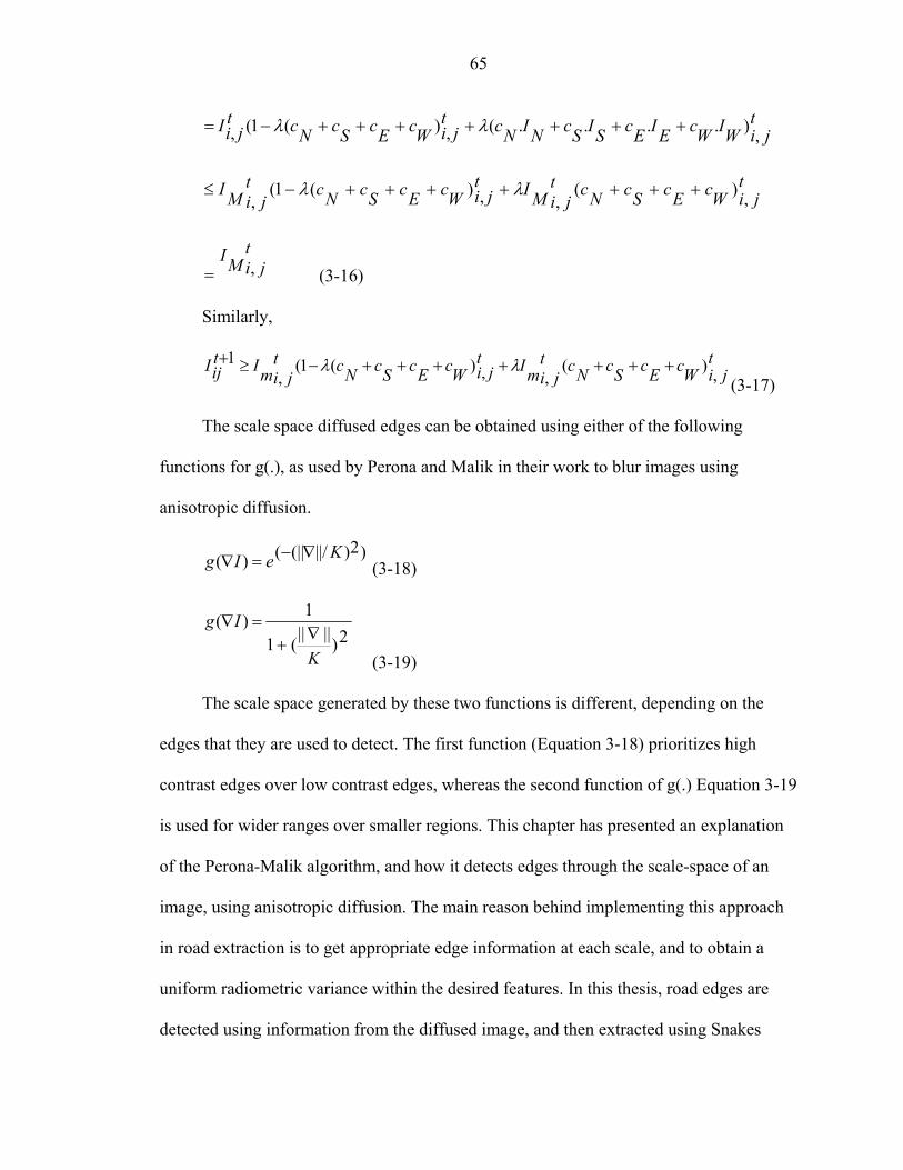
65
tjiWIWcEIEcSIScNINct
jiWcEcScNctjiI ,)....(,)(1(, +++++++−= λλ
tjiWcEcScNct
jiMItjiWcEcScNct
jiMI ,)(,,)(1(
,+++++++−≤ λλ
=t
jiMI, (3-16)
Similarly,
tjiWcEcScNct
jimItjiWcEcScNct
jimItijI ,)(
,,)(1(,
1 +++++++−≥+ λλ(3-17)
The scale space diffused edges can be obtained using either of the following
functions for g(.), as used by Perona and Malik in their work to blur images using
anisotropic diffusion.
)2)/||(||()( KeIg ∇−=∇ (3-18)
2)||||(1
1)(
K
Ig∇
+=∇
(3-19)
The scale space generated by these two functions is different, depending on the
edges that they are used to detect. The first function (Equation 3-18) prioritizes high
contrast edges over low contrast edges, whereas the second function of g(.) Equation 3-19
is used for wider ranges over smaller regions. This chapter has presented an explanation
of the Perona-Malik algorithm, and how it detects edges through the scale-space of an
image, using anisotropic diffusion. The main reason behind implementing this approach
in road extraction is to get appropriate edge information at each scale, and to obtain a
uniform radiometric variance within the desired features. In this thesis, road edges are
detected using information from the diffused image, and then extracted using Snakes

66
(deformable contour models). Snakes, as implemented in this thesis, uses the information
about an edge, gained from the diffused image around the position of each snaxel, in the
process of relocating the snaxels closer to the road edges. A detailed discussion of this
process, with an explanation of the concept of dynamic programming and Snakes, is
provided in Chapter 4. Chapter 4 introduces the working of a Snake, and its
implementation using dynamic programming.
67
CHAPTER 4 SNAKES: THEORY AND IMPLEMENTATION
There are numerous methods to extract road features from an edge detected in an
aerial image. In this research, road feature extraction is performed using Snakes (Kass et
al. 1988) on an image that was pre-processed using the Perona-Malik algorithm (Malik
and Perona, 1990), explained in Chapter 3. Snake is a vector spline representation of a
desired boundary that describes the shape of an object or feature in an image, existing as
a group of edges detected from a pre-processed image. This vector is obtained by
concatenating the snaxels, or points, initially located close to the desired edge of the
feature in the image, and then recursively relocating and concatenating them to align to
the desired shape in the image. In our study, in working toward the objective of
extracting road segment edges from an aerial image, an initial set of road point locations,
or snaxels, are generated and used as inputs to be recursively relocated to get the desired
shape by aligning them to edge over a series of iterations.
The reason behind implementing Snakes on the Perona–Malik algorithm processed
image, is the unique nature of the Perona-Malik algorithm that blurs the image within
regions, while preserving boundaries and edges in the image, as was discussed in Chapter
3. This process retains and further defines the boundaries of the road edges in an image
that is significant in the process of extracting road edges, as it is the edge information that
is needed for Snake’s implementation. According to Kass et al. (1988), Snake is defined
as an energy minimizing spline, guided by external forces and influenced by image forces
68
that pull the spline toward desired objects that are defined and predetermined by the user,
as is discussed in further detail in this chapter.
Snakes. is also called the Active Contour Model; ‘active’ because of its habit of
exhibiting dynamic behavior by recursively relocating the snaxels to align the Snake to
the desired feature in the image. When implementing Snake on an image, the first step in
the process of extracting the desired object is carried out by an initialization, where a set
of points are placed close to the desired feature. This set of points, or snaxels, can be
generated automatically or semi-automatically. In a Semi-automatic approach the user
needs to select the points in or around the vicinity of the desired object, in case of roads,
we need to place points randomly, but close to the road edge features in the image. In the
case of Automatic approaches, the desired features are identified automatically, this
process is followed by the generation of road seeds/points or snaxels.
Snakes relocate the snaxels from their initial positions recursively; they do this by
moving each snaxel individually, to minimize its energy and the overall energy of the
snake so as to get the best possible alignment of the snake to the shape of the desired
feature in the image. This set of points known as snaxels, are iteratively moved closer to
the original location of the edge, using either the dynamic programming or gradient
descent technique to minimize the overall energy of the snake, as will be explained in
detail in Section 4.2.
In what follows is a discussion of the theory and concept behind Snakes and their
implementation. The basic mathematical explanation of Snakes is based on Euler’s
theory, as it is implemented by Kass et al. (1988) and is explained in Section 4.1; their
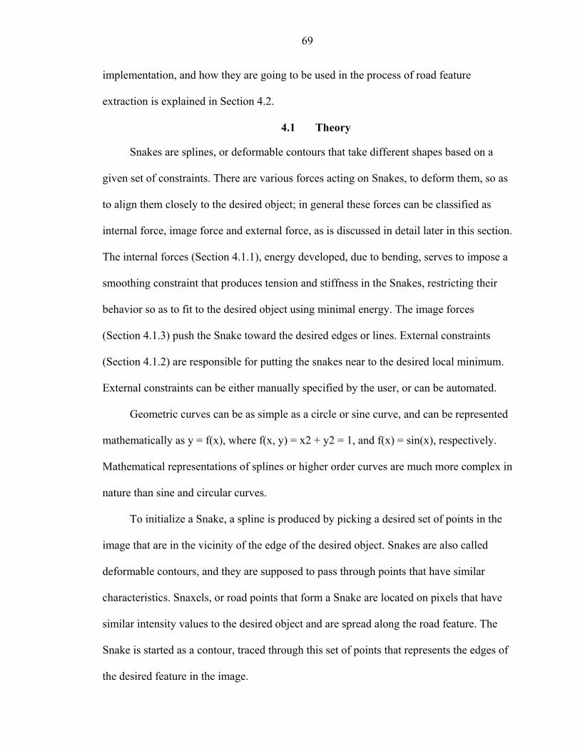
69
implementation, and how they are going to be used in the process of road feature
extraction is explained in Section 4.2.
4.1 Theory
Snakes are splines, or deformable contours that take different shapes based on a
given set of constraints. There are various forces acting on Snakes, to deform them, so as
to align them closely to the desired object; in general these forces can be classified as
internal force, image force and external force, as is discussed in detail later in this section.
The internal forces (Section 4.1.1), energy developed, due to bending, serves to impose a
smoothing constraint that produces tension and stiffness in the Snakes, restricting their
behavior so as to fit to the desired object using minimal energy. The image forces
(Section 4.1.3) push the Snake toward the desired edges or lines. External constraints
(Section 4.1.2) are responsible for putting the snakes near to the desired local minimum.
External constraints can be either manually specified by the user, or can be automated.
Geometric curves can be as simple as a circle or sine curve, and can be represented
mathematically as y = f(x), where f(x, y) = x2 + y2 = 1, and f(x) = sin(x), respectively.
Mathematical representations of splines or higher order curves are much more complex in
nature than sine and circular curves.
To initialize a Snake, a spline is produced by picking a desired set of points in the
image that are in the vicinity of the edge of the desired object. Snakes are also called
deformable contours, and they are supposed to pass through points that have similar
characteristics. Snaxels, or road points that form a Snake are located on pixels that have
similar intensity values to the desired object and are spread along the road feature. The
Snake is started as a contour, traced through this set of points that represents the edges of
the desired feature in the image.
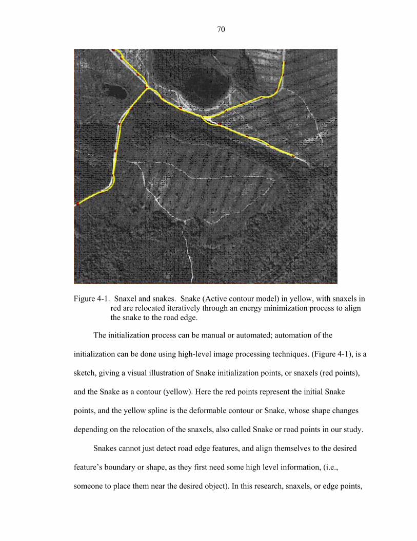
70
Figure 4-1. Snaxel and snakes. Snake (Active contour model) in yellow, with snaxels in
red are relocated iteratively through an energy minimization process to align the snake to the road edge.
The initialization process can be manual or automated; automation of the
initialization can be done using high-level image processing techniques. (Figure 4-1), is a
sketch, giving a visual illustration of Snake initialization points, or snaxels (red points),
and the Snake as a contour (yellow). Here the red points represent the initial Snake
points, and the yellow spline is the deformable contour or Snake, whose shape changes
depending on the relocation of the snaxels, also called Snake or road points in our study.
Snakes cannot just detect road edge features, and align themselves to the desired
feature’s boundary or shape, as they first need some high level information, (i.e.,
someone to place them near the desired object). In this research, snaxels, or edge points,
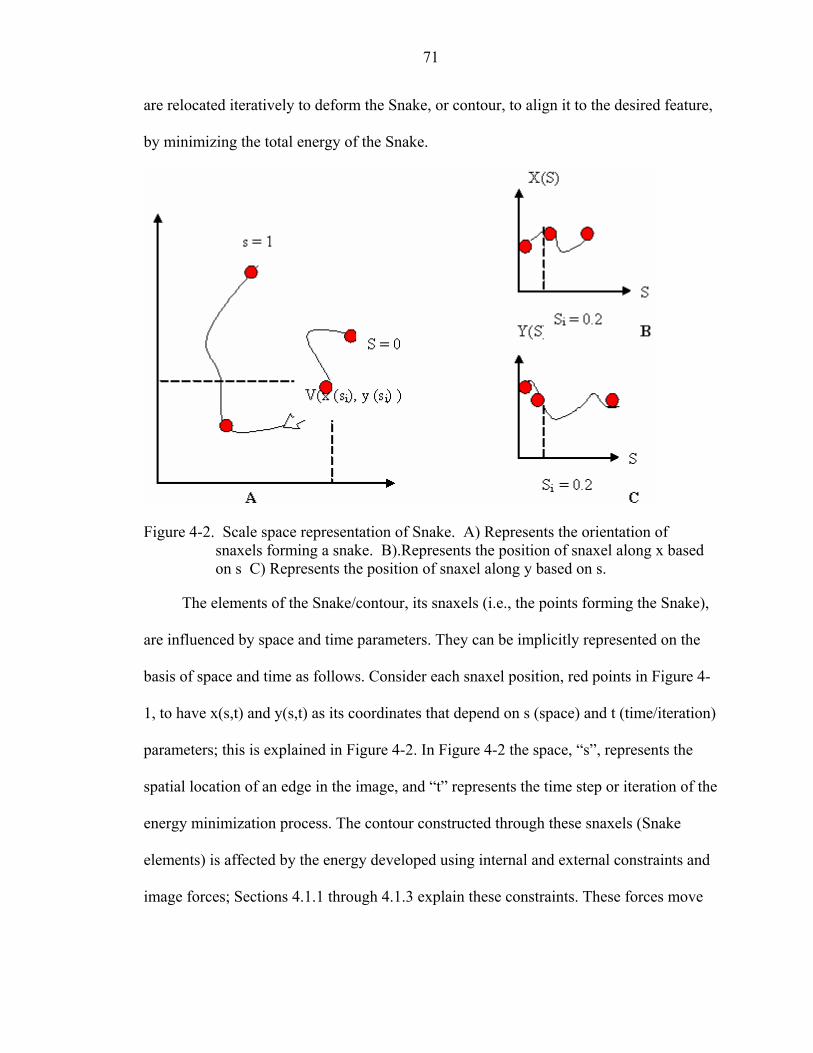
71
are relocated iteratively to deform the Snake, or contour, to align it to the desired feature,
by minimizing the total energy of the Snake.
Figure 4-2. Scale space representation of Snake. A) Represents the orientation of
snaxels forming a snake. B).Represents the position of snaxel along x based on s C) Represents the position of snaxel along y based on s.
The elements of the Snake/contour, its snaxels (i.e., the points forming the Snake),
are influenced by space and time parameters. They can be implicitly represented on the
basis of space and time as follows. Consider each snaxel position, red points in Figure 4-
1, to have x(s,t) and y(s,t) as its coordinates that depend on s (space) and t (time/iteration)
parameters; this is explained in Figure 4-2. In Figure 4-2 the space, “s”, represents the
spatial location of an edge in the image, and “t” represents the time step or iteration of the
energy minimization process. The contour constructed through these snaxels (Snake
elements) is affected by the energy developed using internal and external constraints and
image forces; Sections 4.1.1 through 4.1.3 explain these constraints. These forces move
72
the snaxels over time and space to new coordinates, while minimizing the energy over
each individual snaxel and whole snake.
The objective is to minimize the overall energy to align the Snake to lay over the
desired edge. The energy minimization process allows the Snake to detect the desired
edge. Here, the energy, ESnake, possessed by the contour is the sum of three energy
terms, (i.e., internal, external and image). The total energy, also known as the potential
energy, is the force that makes the Snake move toward the desired edge objects. The
potential energy is used to detect lines, edges, and terminations in the image. The
potential energy developed by the processing of the image is used in Snakes. The total
energy of a Snake is the sum of the energies of the snaxels, that form the snake, or
deformable contour. The position of a snaxel can be parametrically represented as is
shown in Equation 4-1.
))(),(()( sysxsV = (4-1)
Thus, the contour in A (Figure 4-2) can be represented as:
]1,0[,)](),([)( ∈= sTsysxsV (4-2)
Here the Snake represented by Equation 4-2 is composed of a number of snaxels,
who’s locations, (i.e., “x” and “y”) coordinates, are restricted by the value of “s” being
set to fall between 0 and 1. The objective is to align the Snake to the desired object; this
can be obtained by minimizing the total energy of the Snake, (i.e., the sum of the energies
of the individual snaxels) forming the Snake or contour:
dssVelementEsnakeE ))((1
0∫=
(4-3)
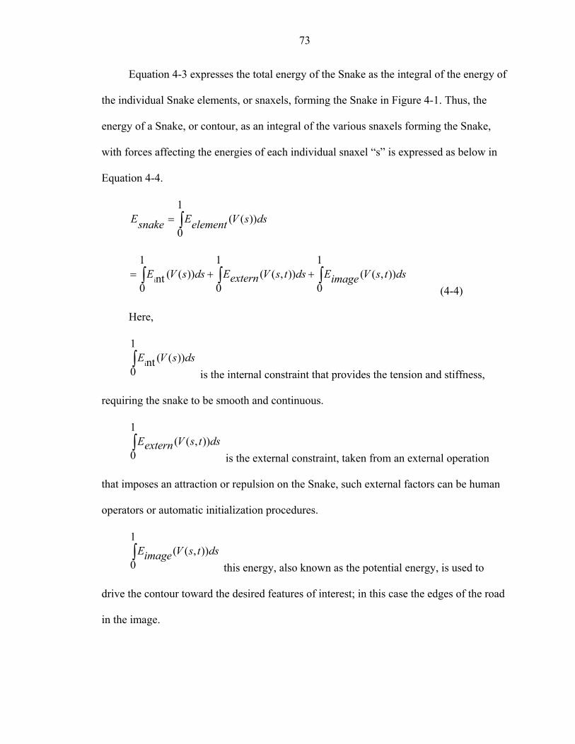
73
Equation 4-3 expresses the total energy of the Snake as the integral of the energy of
the individual Snake elements, or snaxels, forming the Snake in Figure 4-1. Thus, the
energy of a Snake, or contour, as an integral of the various snaxels forming the Snake,
with forces affecting the energies of each individual snaxel “s” is expressed as below in
Equation 4-4.
dssVelementEsnakeE ))((1
0∫=
dstsVimageEdstsVexternEdssVE )),((1
0)),((
1
0))((
1
0nti ∫∫∫ ++=
(4-4)
Here,
dssVE ))((1
0nti∫
is the internal constraint that provides the tension and stiffness,
requiring the snake to be smooth and continuous.
dstsVexternE )),((1
0∫
is the external constraint, taken from an external operation
that imposes an attraction or repulsion on the Snake, such external factors can be human
operators or automatic initialization procedures.
dstsVimageE )),((1
0∫
this energy, also known as the potential energy, is used to
drive the contour toward the desired features of interest; in this case the edges of the road
in the image.
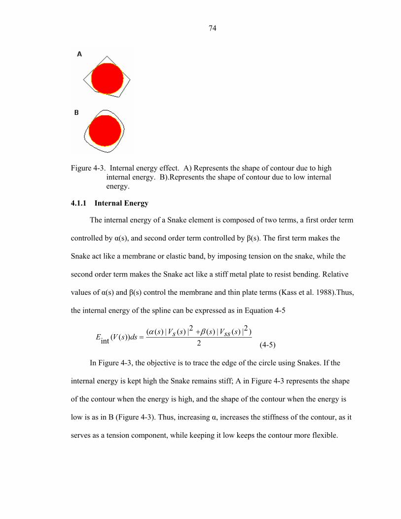
74
Figure 4-3. Internal energy effect. A) Represents the shape of contour due to high
internal energy. B).Represents the shape of contour due to low internal energy.
4.1.1 Internal Energy
The internal energy of a Snake element is composed of two terms, a first order term
controlled by α(s), and second order term controlled by β(s). The first term makes the
Snake act like a membrane or elastic band, by imposing tension on the snake, while the
second order term makes the Snake act like a stiff metal plate to resist bending. Relative
values of α(s) and β(s) control the membrane and thin plate terms (Kass et al. 1988).Thus,
the internal energy of the spline can be expressed as in Equation 4-5
2)2|)(|)(2|)(|)((
))((intsssVsssVs
dssVEβα +
= (4-5)
In Figure 4-3, the objective is to trace the edge of the circle using Snakes. If the
internal energy is kept high the Snake remains stiff; A in Figure 4-3 represents the shape
of the contour when the energy is high, and the shape of the contour when the energy is
low is as in B (Figure 4-3). Thus, increasing α, increases the stiffness of the contour, as it
serves as a tension component, while keeping it low keeps the contour more flexible.
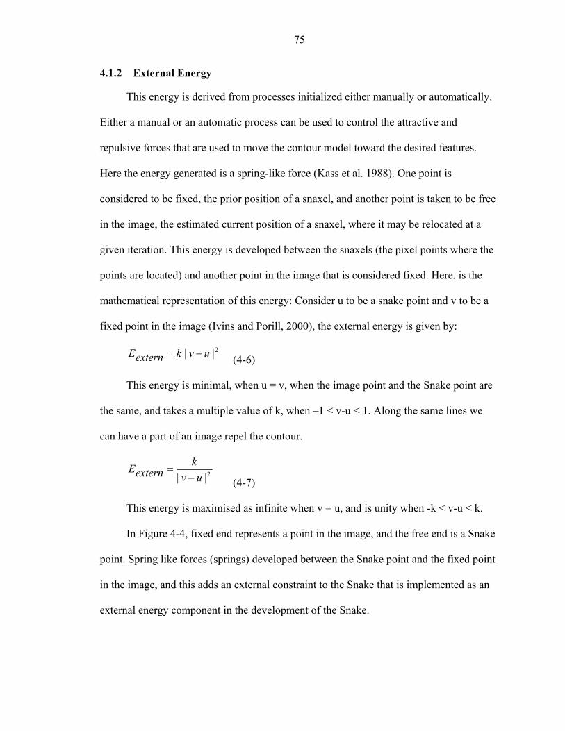
75
4.1.2 External Energy
This energy is derived from processes initialized either manually or automatically.
Either a manual or an automatic process can be used to control the attractive and
repulsive forces that are used to move the contour model toward the desired features.
Here the energy generated is a spring-like force (Kass et al. 1988). One point is
considered to be fixed, the prior position of a snaxel, and another point is taken to be free
in the image, the estimated current position of a snaxel, where it may be relocated at a
given iteration. This energy is developed between the snaxels (the pixel points where the
points are located) and another point in the image that is considered fixed. Here, is the
mathematical representation of this energy: Consider u to be a snake point and v to be a
fixed point in the image (Ivins and Porill, 2000), the external energy is given by:
2|| uvkexternE −= (4-6)
This energy is minimal, when u = v, when the image point and the Snake point are
the same, and takes a multiple value of k, when –1 < v-u < 1. Along the same lines we
can have a part of an image repel the contour.
2|| uvk
externE−
= (4-7)
This energy is maximised as infinite when v = u, and is unity when -k < v-u < k.
In Figure 4-4, fixed end represents a point in the image, and the free end is a Snake
point. Spring like forces (springs) developed between the Snake point and the fixed point
in the image, and this adds an external constraint to the Snake that is implemented as an
external energy component in the development of the Snake.
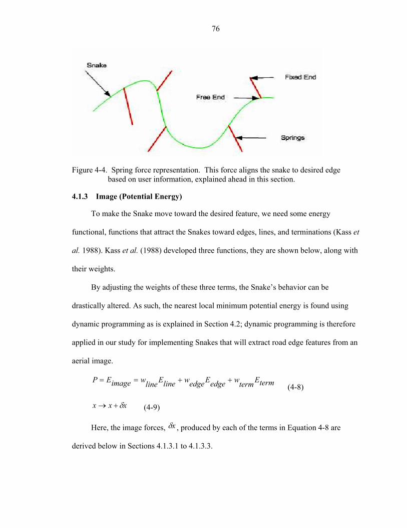
76
Figure 4-4. Spring force representation. This force aligns the snake to desired edge
based on user information, explained ahead in this section.
4.1.3 Image (Potential Energy)
To make the Snake move toward the desired feature, we need some energy
functional, functions that attract the Snakes toward edges, lines, and terminations (Kass et
al. 1988). Kass et al. (1988) developed three functions, they are shown below, along with
their weights.
By adjusting the weights of these three terms, the Snake’s behavior can be
drastically altered. As such, the nearest local minimum potential energy is found using
dynamic programming as is explained in Section 4.2; dynamic programming is therefore
applied in our study for implementing Snakes that will extract road edge features from an
aerial image.
termEtermwedgeEedgewlineElinewimageEP ++== (4-8)
xxx δ+→ (4-9)
Here, the image forces, xδ , produced by each of the terms in Equation 4-8 are
derived below in Sections 4.1.3.1 to 4.1.3.3.
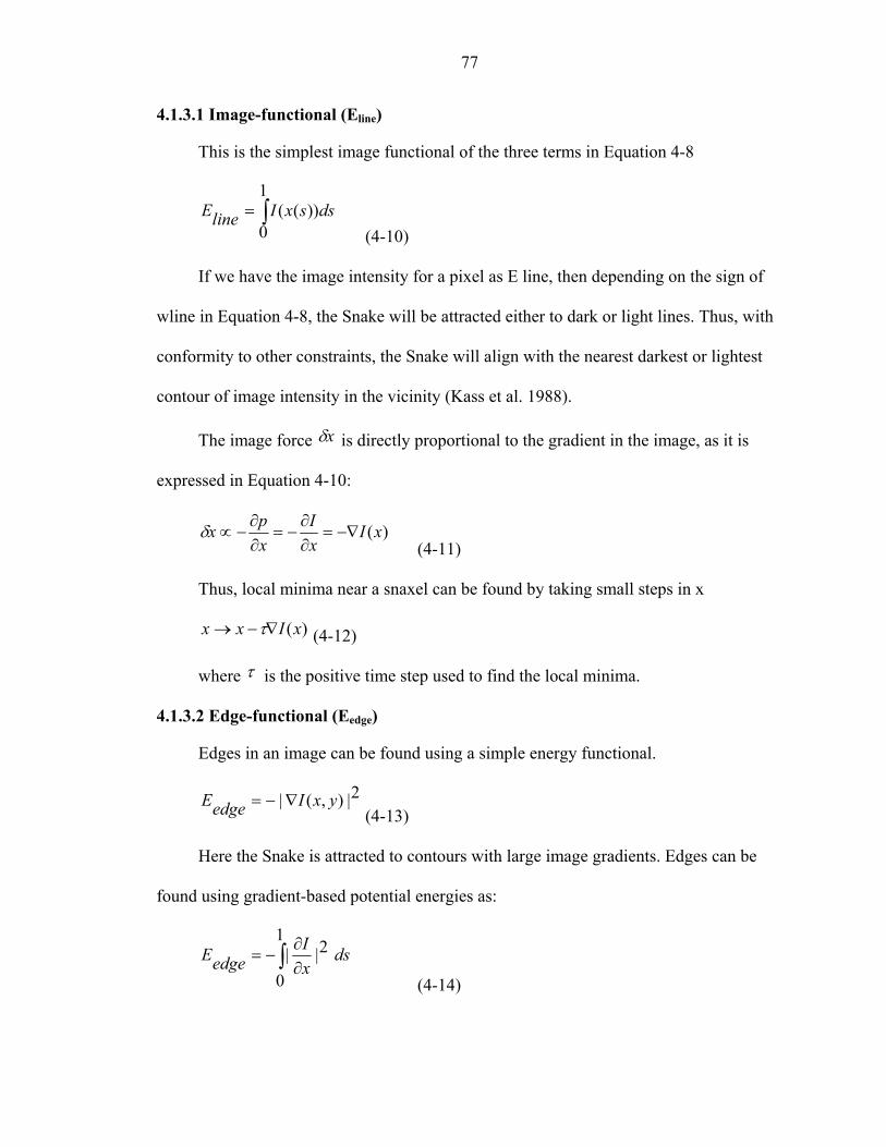
77
4.1.3.1 Image-functional (Eline)
This is the simplest image functional of the three terms in Equation 4-8
∫=1
0))(( dssxIlineE
(4-10)
If we have the image intensity for a pixel as E line, then depending on the sign of
wline in Equation 4-8, the Snake will be attracted either to dark or light lines. Thus, with
conformity to other constraints, the Snake will align with the nearest darkest or lightest
contour of image intensity in the vicinity (Kass et al. 1988).
The image force xδ is directly proportional to the gradient in the image, as it is
expressed in Equation 4-10:
)(xIxI
xpx −∇=
∂∂
−=∂∂
−∝δ (4-11)
Thus, local minima near a snaxel can be found by taking small steps in x
)(xIxx ∇−→ τ (4-12)
where τ is the positive time step used to find the local minima.
4.1.3.2 Edge-functional (Eedge)
Edges in an image can be found using a simple energy functional.
2|),(| yxIedgeE ∇−= (4-13)
Here the Snake is attracted to contours with large image gradients. Edges can be
found using gradient-based potential energies as:
dsxI
edgeE 2|1
0|∫ ∂∂
−=
(4-14)
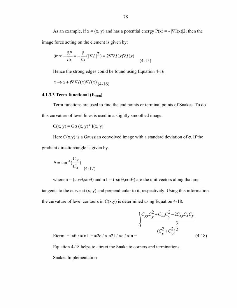
78
As an example, if x = (x, y) and has a potential energy P(x) = - |∇I(x)|2; then the
image force acting on the element is given by:
)()(2)2|(| xIxIIxx
Px ∇∇∇=∇∂∂
−=∂∂
−∝δ (4-15)
Hence the strong edges could be found using Equation 4-16
)()( xIxIxx ∇∇∇+→ τ (4-16)
4.1.3.3 Term-functional (Eterm)
Term functions are used to find the end points or terminal points of Snakes. To do
this curvature of level lines is used in a slightly smoothed image.
C(x, y) = Gσ (x, y)* I(x, y)
Here C(x,y) is a Gaussian convolved image with a standard deviation of σ. If the
gradient direction/angle is given by.
)(tan 1
xCyC
−=θ (4-17)
where n = (cosθ,sinθ) and n⊥ = (-sinθ,cosθ) are the unit vectors along that are
tangents to the curve at (x, y) and perpendicular to it, respectively. Using this information
the curvature of level contours in C(x,y) is determined using Equation 4-18.
Eterm = ≈θ / ≈ n⊥ = ≈2c / ≈ n2⊥/ ≈c / ≈ n =
∫+
−+1
023
)22(
222
yCxC
yCxCxyCyCxxCxCyyC
(4-18)
Equation 4-18 helps to attract the Snake to corners and terminations.
Snakes Implementation
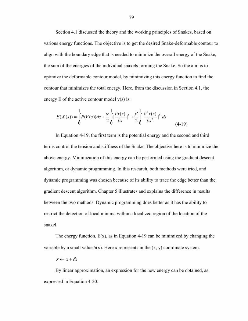
79
Section 4.1 discussed the theory and the working principles of Snakes, based on
various energy functions. The objective is to get the desired Snake-deformable contour to
align with the boundary edge that is needed to minimize the overall energy of the Snake,
the sum of the energies of the individual snaxels forming the Snake. So the aim is to
optimize the deformable contour model, by minimizing this energy function to find the
contour that minimizes the total energy. Here, from the discussion in Section 4.1, the
energy E of the active contour model v(s) is:
dss
sxssxdssVPsXE 2
2
22 |
1
0
)(|2
|1
0
1
0
)(|2
))(())(( ∫∫ ∫ ∂∂
+∂
∂+=
βα
(4-19)
In Equation 4-19, the first term is the potential energy and the second and third
terms control the tension and stiffness of the Snake. The objective here is to minimize the
above energy. Minimization of this energy can be performed using the gradient descent
algorithm, or dynamic programming. In this research, both methods were tried, and
dynamic programming was chosen because of its ability to trace the edge better than the
gradient descent algorithm. Chapter 5 illustrates and explains the difference in results
between the two methods. Dynamic programming does better as it has the ability to
restrict the detection of local minima within a localized region of the location of the
snaxel.
The energy function, E(x), as in Equation 4-19 can be minimized by changing the
variable by a small value δ(x). Here x represents in the (x, y) coordinate system.
xxx δ+←
By linear approximation, an expression for the new energy can be obtained, as
expressed in Equation 4-20.
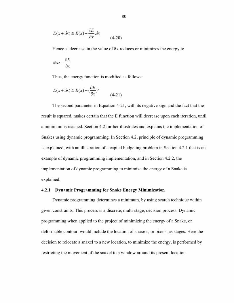
80
xxExExxE δδ .)()(∂∂
+≅+ (4-20)
Hence, a decrease in the value of δx reduces or minimizes the energy.to
xEx∂∂
−αδ
Thus, the energy function is modified as follows:
2)()()(xExExxE∂∂
−≅+δ (4-21)
The second parameter in Equation 4-21, with its negative sign and the fact that the
result is squared, makes certain that the E function will decrease upon each iteration, until
a minimum is reached. Section 4.2 further illustrates and explains the implementation of
Snakes using dynamic programming. In Section 4.2, principle of dynamic programming
is explained, with an illustration of a capital budgeting problem in Section 4.2.1 that is an
example of dynamic programming implementation, and in Section 4.2.2, the
implementation of dynamic programming to minimize the energy of a Snake is
explained.
4.2.1 Dynamic Programming for Snake Energy Minimization
Dynamic programming determines a minimum, by using search technique within
given constraints. This process is a discrete, multi-stage, decision process. Dynamic
programming when applied to the project of minimizing the energy of a Snake, or
deformable contour, would include the location of snaxels, or pixels, as stages. Here the
decision to relocate a snaxel to a new location, to minimize the energy, is performed by
restricting the movement of the snaxel to a window around its present location.
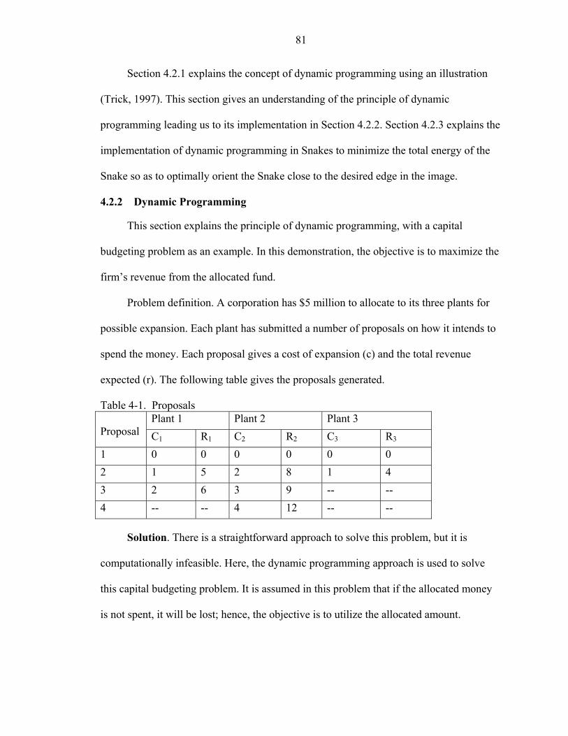
81
Section 4.2.1 explains the concept of dynamic programming using an illustration
(Trick, 1997). This section gives an understanding of the principle of dynamic
programming leading us to its implementation in Section 4.2.2. Section 4.2.3 explains the
implementation of dynamic programming in Snakes to minimize the total energy of the
Snake so as to optimally orient the Snake close to the desired edge in the image.
4.2.2 Dynamic Programming
This section explains the principle of dynamic programming, with a capital
budgeting problem as an example. In this demonstration, the objective is to maximize the
firm’s revenue from the allocated fund.
Problem definition. A corporation has $5 million to allocate to its three plants for
possible expansion. Each plant has submitted a number of proposals on how it intends to
spend the money. Each proposal gives a cost of expansion (c) and the total revenue
expected (r). The following table gives the proposals generated.
Table 4-1. Proposals Plant 1 Plant 2 Plant 3
Proposal C1 R1 C2 R2 C3 R3 1 0 0 0 0 0 0 2 1 5 2 8 1 4 3 2 6 3 9 -- -- 4 -- -- 4 12 -- --
Solution. There is a straightforward approach to solve this problem, but it is
computationally infeasible. Here, the dynamic programming approach is used to solve
this capital budgeting problem. It is assumed in this problem that if the allocated money
is not spent, it will be lost; hence, the objective is to utilize the allocated amount.

82
The problem is split into three stages, each stage representing the money allocated
to each plant. Thus, stage 1 represents money allocated to Plant 1, stage 2 and 3
representing money allocated to Plants 2 and 3 respectively. In this approach the order of
allocation is first set to Plant 1 and then to Plant 2 and 3 respectively.
Each stage is further divided into states. A state includes the information required
to go from one stage to the next. In this case the states for stages 1, 2 and 3 are as follows.
{0, 1, 2, 3, 4, 5}: Amount of money spent on Plant 1, as x1,
{0, 1, 2, 3, 4, 5}: Amount of money spent on Plants 1 and 2, as x2, and
{5}: Amount of money spent on Plants 1, 2 and 3 as x3
Thus, each stage is associated with revenue, and to make a decision at Stage 3, only
the amount spent on Plants 1 and 2 needs to be known. As can be seen from the states
above, in states x1 and x2, we have a set of options for the amount that can be invested.
Whereas in the case of state x3 we only have an option of 5, as the total amount invested
in the Plants 1, 2 and 3 must be equal to $5 million. Since we cannot spend above it, nor
can we spend less than $5 million dollars, if we do not spend the allocated amount, it will
be lost as per problem definition.
Table 4-2. Stage 1 computation If Capital Available (x1) Then Optimal Proposal And revenue for Stage 1 0 1 0 1 2 5 2 3 6 3 3 6 4 3 6 5 3 6
The following computation at each stage illustrates the working principle of
dynamic programming. In Table 4-2, we have an option to select from the set of capital
available (x1), for an optimal proposal, and the revenue from them invested in Plant 1,

83
inferred from Table 4-1. Further, this process evaluates the best solution for Plants 1 and
2 in Stage 2, with a number of pre-defined options for states being represented by x2.
At Stage 2, to calculate the best revenue for a given state x2, this process goes
through all the Plant 2 proposals, and allocates the amount of funds to Plant 2 and then
the remainder of the amount is optimally used for Plant 1, based on the information from
Table 4-2. This example further illustrates the above discussion: suppose the best
allocation for the state x2 = 4, then in Stage 2, one of the following proposals could be
implemented.
From Table 4-1, if we select a particular proposal for Plant 2 in Stage 2, the
remainder of the amount invested from Stage 2 is utilized for Plant 1. Table 4.3 below
illustrates the total revenue based on the combination of the proposals for Plants 1 and 2.
Table 4-3. Proposal revenue combination If Plant 2 proposal
Then Plant 2 Revenue
Then Funds remaining For Stage 1
Maximum revenue From Stage 1
Total revenue from Plant 1 and 2
1 0 4 6 6 2 8 2 6 14 3 9 1 5 14 4 12 0 0 12
Thus, the best proposal to be selected for Plants 1 and 2, would be either proposal 1
for Plant 2 and proposal 2 for Plant 1, returning a revenue of 14, or proposal 2 for Plant 2
and proposal 1 for Plant 1, also returning a revenue of 14. Further Table 4.4 illustrates the
set of options available for state x2 in Stage 2, with the corresponding optimal proposals
for each of the options, and the total revenue return from Stages 1 and 2. Below, Stage 3
is considered, with only one option for the state x3 = 5.
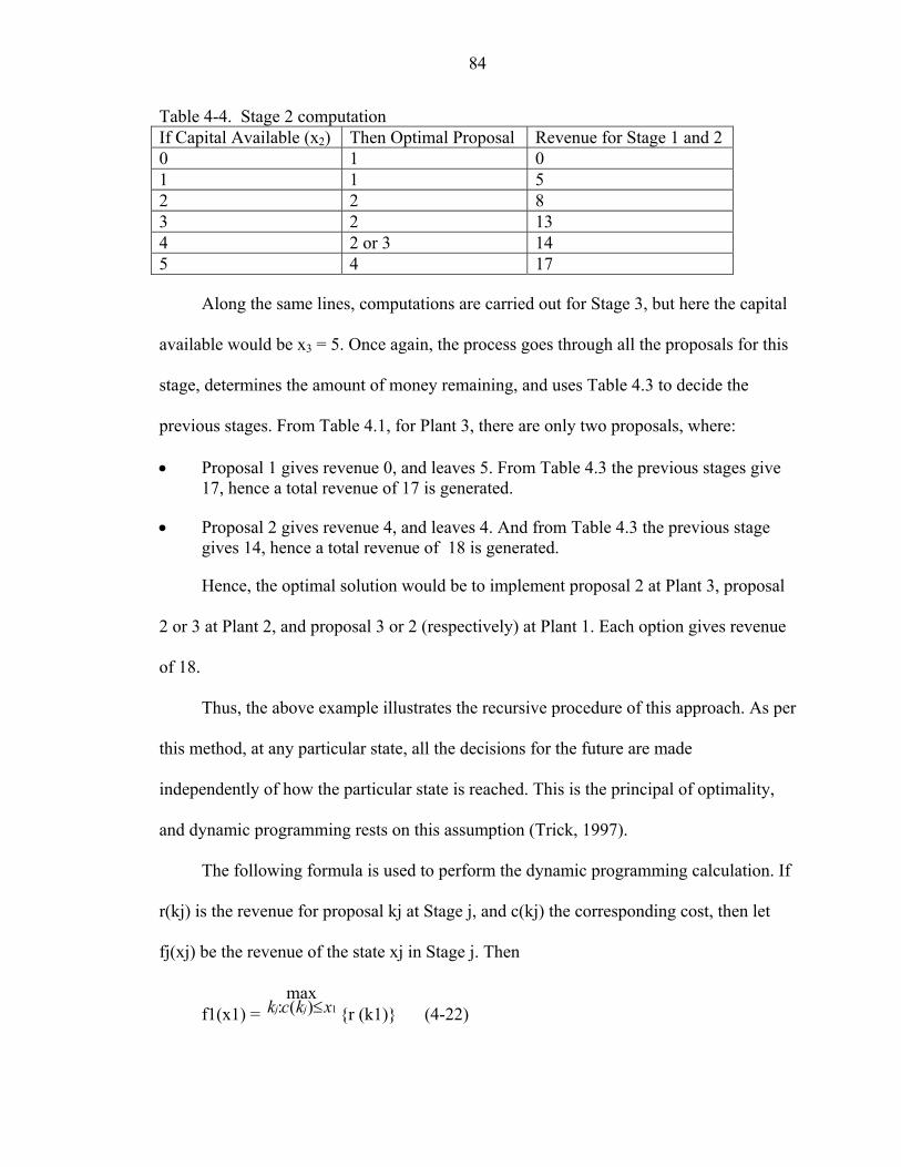
84
Table 4-4. Stage 2 computation If Capital Available (x2) Then Optimal Proposal Revenue for Stage 1 and 2 0 1 0 1 1 5 2 2 8 3 2 13 4 2 or 3 14 5 4 17
Along the same lines, computations are carried out for Stage 3, but here the capital
available would be x3 = 5. Once again, the process goes through all the proposals for this
stage, determines the amount of money remaining, and uses Table 4.3 to decide the
previous stages. From Table 4.1, for Plant 3, there are only two proposals, where:
• Proposal 1 gives revenue 0, and leaves 5. From Table 4.3 the previous stages give 17, hence a total revenue of 17 is generated.
• Proposal 2 gives revenue 4, and leaves 4. And from Table 4.3 the previous stage gives 14, hence a total revenue of 18 is generated.
Hence, the optimal solution would be to implement proposal 2 at Plant 3, proposal
2 or 3 at Plant 2, and proposal 3 or 2 (respectively) at Plant 1. Each option gives revenue
of 18.
Thus, the above example illustrates the recursive procedure of this approach. As per
this method, at any particular state, all the decisions for the future are made
independently of how the particular state is reached. This is the principal of optimality,
and dynamic programming rests on this assumption (Trick, 1997).
The following formula is used to perform the dynamic programming calculation. If
r(kj) is the revenue for proposal kj at Stage j, and c(kj) the corresponding cost, then let
fj(xj) be the revenue of the state xj in Stage j. Then
f1(x1) = max
)(: 1xkck jj ≤ {r (k1)} (4-22)

85
and
fj(xj) = max
)(: jjj xkck ≤ {r(kj) + fj-1(xj – c(kj))} for j = 2, 3 (4-23)
This formula is used to compute the revenue function in the forward procedure; it is
also possible to compute it in a backward procedure that gives the same result. Using the
same principle, dynamic programming is implemented in the next section for the energy
minimization of Snakes.
4.2.3 Dynamic Snake Implementation
In an analogous way to the implementation in Section 4.2.2, the snaxels, point
locations along the Snake, are relocated in the deformable model based on the energy
minimization procedure. This is done in a similar fashion to the states of revenue in Stage
1, as was explained in Section 4.2.2. In Section 4.2.2, the revenue was restricted to a
maximum of $5 million, in Snakes, the movement of a snaxel is restricted to a search
window around its current position. The objective of the process is to minimize the total
energy, by minimizing the energy at each stage ( i.e., at each snaxel location in the
model). Figure 4-5, illustrates the movement a snaxel in its vicinity search window, and
the changing orientation of the Snake. Here, each snaxel is analogous to a stage and the
positions in the search window represent the states.
At any snaxel position, the energy is given by the sum of the energies at the
preceding position and the current snaxel position. The minimal sum of these energies is
retained as the optimal value. The process continues through all the snaxels, and at the
end of each iteration of the minimization process, the points, or snaxels, move toward
those new locations that generated the optimal path in each of their neighborhoods, as is
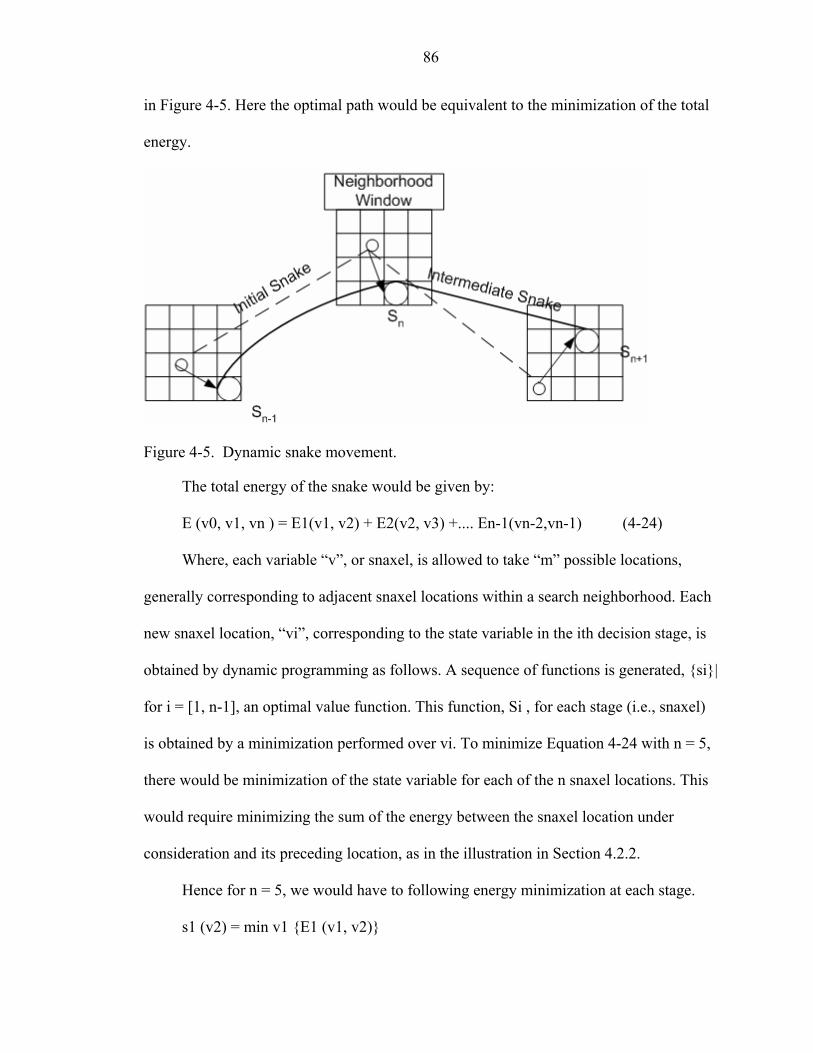
86
in Figure 4-5. Here the optimal path would be equivalent to the minimization of the total
energy.
Figure 4-5. Dynamic snake movement.
The total energy of the snake would be given by:
E (v0, v1, vn ) = E1(v1, v2) + E2(v2, v3) +.... En-1(vn-2,vn-1) (4-24)
Where, each variable “v”, or snaxel, is allowed to take “m” possible locations,
generally corresponding to adjacent snaxel locations within a search neighborhood. Each
new snaxel location, “vi”, corresponding to the state variable in the ith decision stage, is
obtained by dynamic programming as follows. A sequence of functions is generated, {si}|
for i = [1, n-1], an optimal value function. This function, Si , for each stage (i.e., snaxel)
is obtained by a minimization performed over vi. To minimize Equation 4-24 with n = 5,
there would be minimization of the state variable for each of the n snaxel locations. This
would require minimizing the sum of the energy between the snaxel location under
consideration and its preceding location, as in the illustration in Section 4.2.2.
Hence for n = 5, we would have to following energy minimization at each stage.
s1 (v2) = min v1 {E1 (v1, v2)}
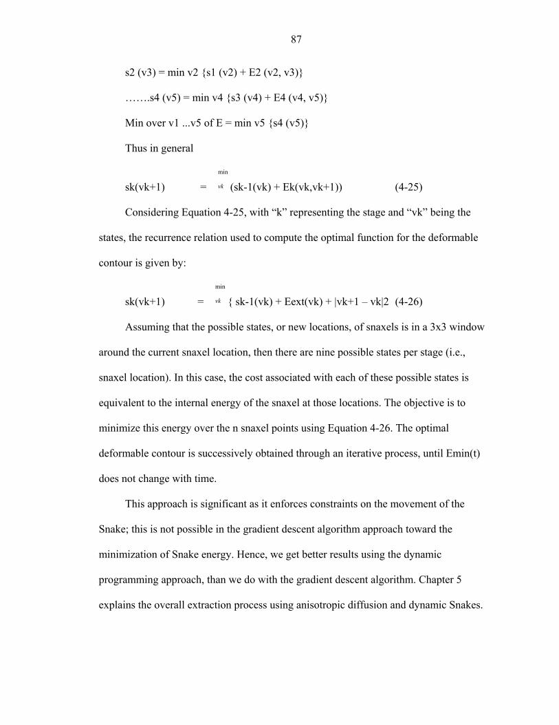
87
s2 (v3) = min v2 {s1 (v2) + E2 (v2, v3)}
…….s4 (v5) = min v4 {s3 (v4) + E4 (v4, v5)}
Min over v1 ...v5 of E = min v5 {s4 (v5)}
Thus in general
sk(vk+1) = min
vk (sk-1(vk) + Ek(vk,vk+1)) (4-25)
Considering Equation 4-25, with “k” representing the stage and “vk” being the
states, the recurrence relation used to compute the optimal function for the deformable
contour is given by:
sk(vk+1) = min
vk { sk-1(vk) + Eext(vk) + |vk+1 – vk|2 (4-26)
Assuming that the possible states, or new locations, of snaxels is in a 3x3 window
around the current snaxel location, then there are nine possible states per stage (i.e.,
snaxel location). In this case, the cost associated with each of these possible states is
equivalent to the internal energy of the snaxel at those locations. The objective is to
minimize this energy over the n snaxel points using Equation 4-26. The optimal
deformable contour is successively obtained through an iterative process, until Emin(t)
does not change with time.
This approach is significant as it enforces constraints on the movement of the
Snake; this is not possible in the gradient descent algorithm approach toward the
minimization of Snake energy. Hence, we get better results using the dynamic
programming approach, than we do with the gradient descent algorithm. Chapter 5
explains the overall extraction process using anisotropic diffusion and dynamic Snakes.
88
CHAPTER 5 METHOD OF EXTRACTION
Numerous methods exist to extract road features from an aerial image. Most of the
feature extraction methods that are developed are implemented using a combination of
image processing techniques, from various levels of an image processing system. Road
representation varies from image to image depending on the resolution of the image, the
weather conditions prevailing at the time of photograph, and the sun’s position, as was
discussed in Chapter 2. Hence, it is very difficult to have a common method to extract the
roads from any image. To overcome the hurdle of implementing new methods to identify
and extract road features from any aerial image, depending on the nature of the image,
research in the recent past was targeted toward developing a global method, using a
combination of image processing techniques to extract road features from any aerial
image.
Our study has developed a feature extraction method that could be implemented as
an initial road extraction method in a global model, or as an independent semi-automatic
road extraction method. This method evolved through stages, with implementation of the
Perona-Malik algorithm and Snakes (Deformable Contour Models) using dynamic
programming. Section 5.3 explains in detail this stage based on evolution of the method
over stages in the process of development, and is followed by a detailed explanation of
the implemented method of road feature extraction.
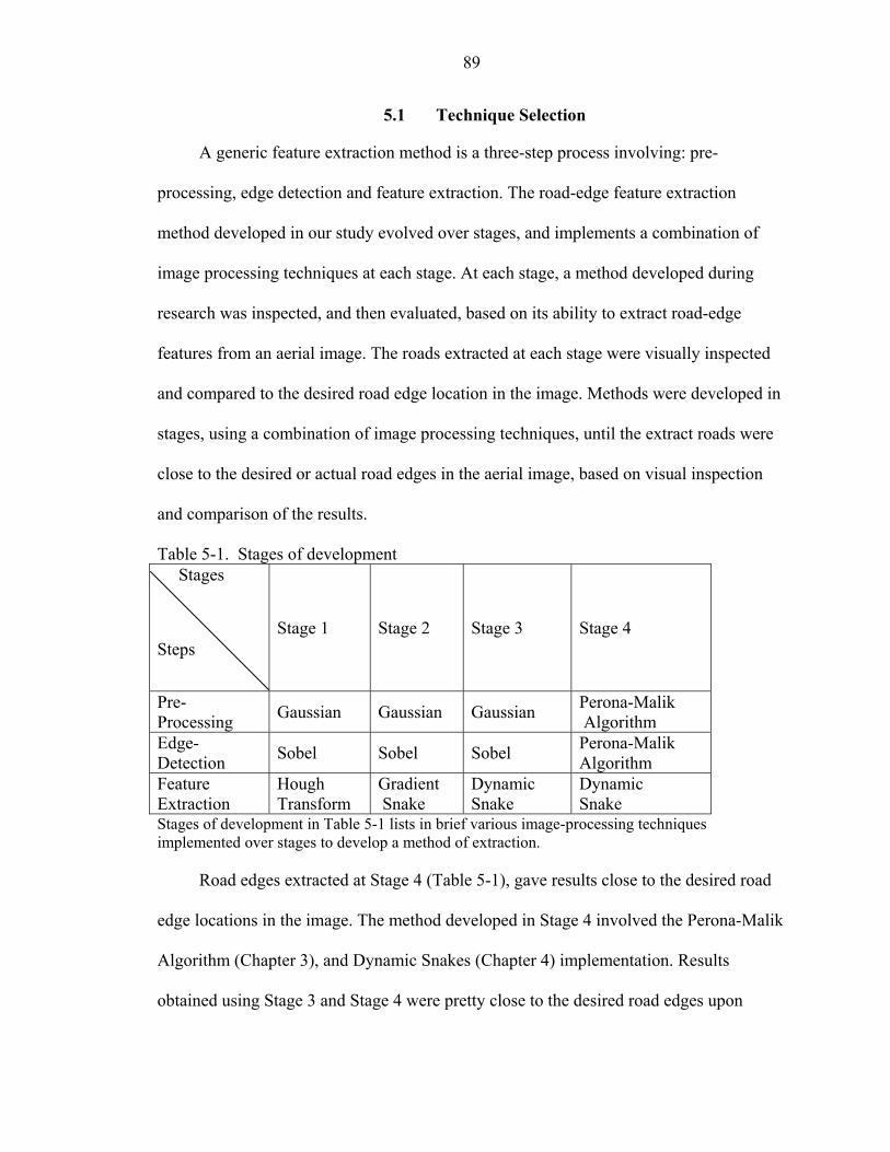
89
5.1 Technique Selection
A generic feature extraction method is a three-step process involving: pre-
processing, edge detection and feature extraction. The road-edge feature extraction
method developed in our study evolved over stages, and implements a combination of
image processing techniques at each stage. At each stage, a method developed during
research was inspected, and then evaluated, based on its ability to extract road-edge
features from an aerial image. The roads extracted at each stage were visually inspected
and compared to the desired road edge location in the image. Methods were developed in
stages, using a combination of image processing techniques, until the extract roads were
close to the desired or actual road edges in the aerial image, based on visual inspection
and comparison of the results.
Table 5-1. Stages of development Stages
Steps Stage 1 Stage 2 Stage 3 Stage 4
Pre-Processing Gaussian Gaussian Gaussian Perona-Malik
Algorithm Edge-Detection Sobel Sobel Sobel Perona-Malik
Algorithm Feature Extraction
Hough Transform
Gradient Snake
Dynamic Snake
Dynamic Snake
Stages of development in Table 5-1 lists in brief various image-processing techniques implemented over stages to develop a method of extraction.
Road edges extracted at Stage 4 (Table 5-1), gave results close to the desired road
edge locations in the image. The method developed in Stage 4 involved the Perona-Malik
Algorithm (Chapter 3), and Dynamic Snakes (Chapter 4) implementation. Results
obtained using Stage 3 and Stage 4 were pretty close to the desired road edges upon
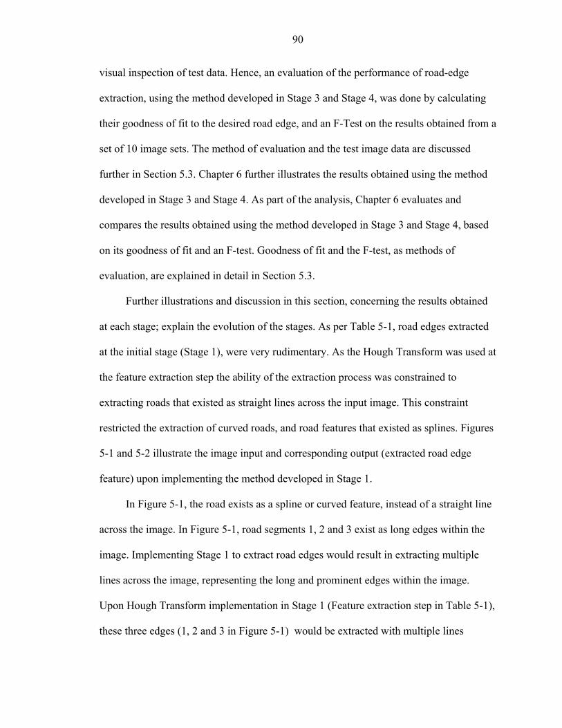
90
visual inspection of test data. Hence, an evaluation of the performance of road-edge
extraction, using the method developed in Stage 3 and Stage 4, was done by calculating
their goodness of fit to the desired road edge, and an F-Test on the results obtained from a
set of 10 image sets. The method of evaluation and the test image data are discussed
further in Section 5.3. Chapter 6 further illustrates the results obtained using the method
developed in Stage 3 and Stage 4. As part of the analysis, Chapter 6 evaluates and
compares the results obtained using the method developed in Stage 3 and Stage 4, based
on its goodness of fit and an F-test. Goodness of fit and the F-test, as methods of
evaluation, are explained in detail in Section 5.3.
Further illustrations and discussion in this section, concerning the results obtained
at each stage; explain the evolution of the stages. As per Table 5-1, road edges extracted
at the initial stage (Stage 1), were very rudimentary. As the Hough Transform was used at
the feature extraction step the ability of the extraction process was constrained to
extracting roads that existed as straight lines across the input image. This constraint
restricted the extraction of curved roads, and road features that existed as splines. Figures
5-1 and 5-2 illustrate the image input and corresponding output (extracted road edge
feature) upon implementing the method developed in Stage 1.
In Figure 5-1, the road exists as a spline or curved feature, instead of a straight line
across the image. In Figure 5-1, road segments 1, 2 and 3 exist as long edges within the
image. Implementing Stage 1 to extract road edges would result in extracting multiple
lines across the image, representing the long and prominent edges within the image.
Upon Hough Transform implementation in Stage 1 (Feature extraction step in Table 5-1),
these three edges (1, 2 and 3 in Figure 5-1) would be extracted with multiple lines
91
passing through them, as many lines in Hough space (Chapter 2) would have edge pixels
forming the road edges for Sections 1, 2 and 3 passing through them.
Figure 5-1. Input image for Hough transform.
Figure 5-2 illustrates the road extracted using the Hough Transform from the input
image in Figure 5-1. Thus following the principle of the Hough Transform, the lines
passing through the maximum number of edge pixels are traced. The results obtained
using the method developed in Stage 1 require a lot of post-processing, involving
selection of the best fit line, trimming the line to fit actual road segments in the image and
linking the extracted segments. All considered, roads extracted using the Hough
transform will not align to the curves and spline road features, and would require
alternative image processing techniques to extract curves and splines. Hence, Active
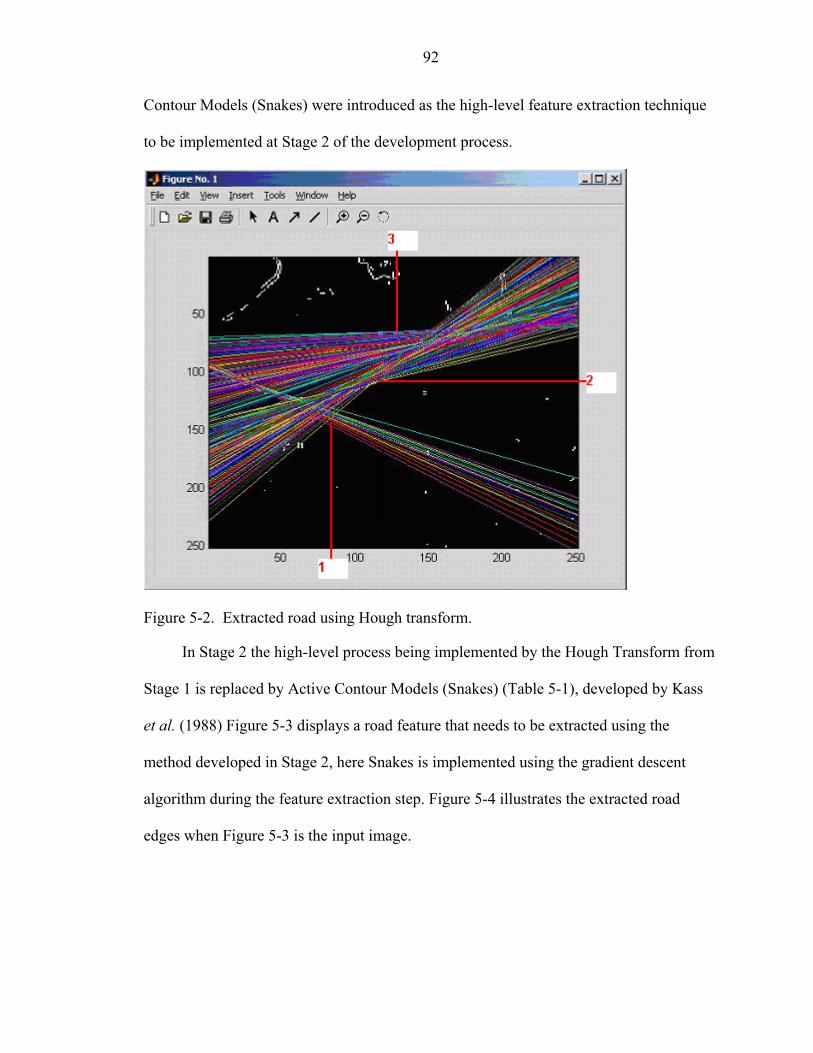
92
Contour Models (Snakes) were introduced as the high-level feature extraction technique
to be implemented at Stage 2 of the development process.
Figure 5-2. Extracted road using Hough transform.
In Stage 2 the high-level process being implemented by the Hough Transform from
Stage 1 is replaced by Active Contour Models (Snakes) (Table 5-1), developed by Kass
et al. (1988) Figure 5-3 displays a road feature that needs to be extracted using the
method developed in Stage 2, here Snakes is implemented using the gradient descent
algorithm during the feature extraction step. Figure 5-4 illustrates the extracted road
edges when Figure 5-3 is the input image.
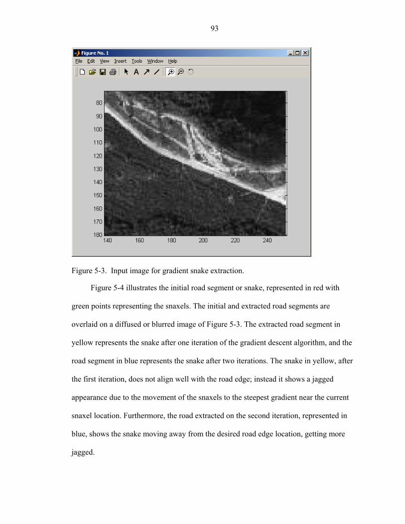
93
Figure 5-3. Input image for gradient snake extraction.
Figure 5-4 illustrates the initial road segment or snake, represented in red with
green points representing the snaxels. The initial and extracted road segments are
overlaid on a diffused or blurred image of Figure 5-3. The extracted road segment in
yellow represents the snake after one iteration of the gradient descent algorithm, and the
road segment in blue represents the snake after two iterations. The snake in yellow, after
the first iteration, does not align well with the road edge; instead it shows a jagged
appearance due to the movement of the snaxels to the steepest gradient near the current
snaxel location. Furthermore, the road extracted on the second iteration, represented in
blue, shows the snake moving away from the desired road edge location, getting more
jagged.
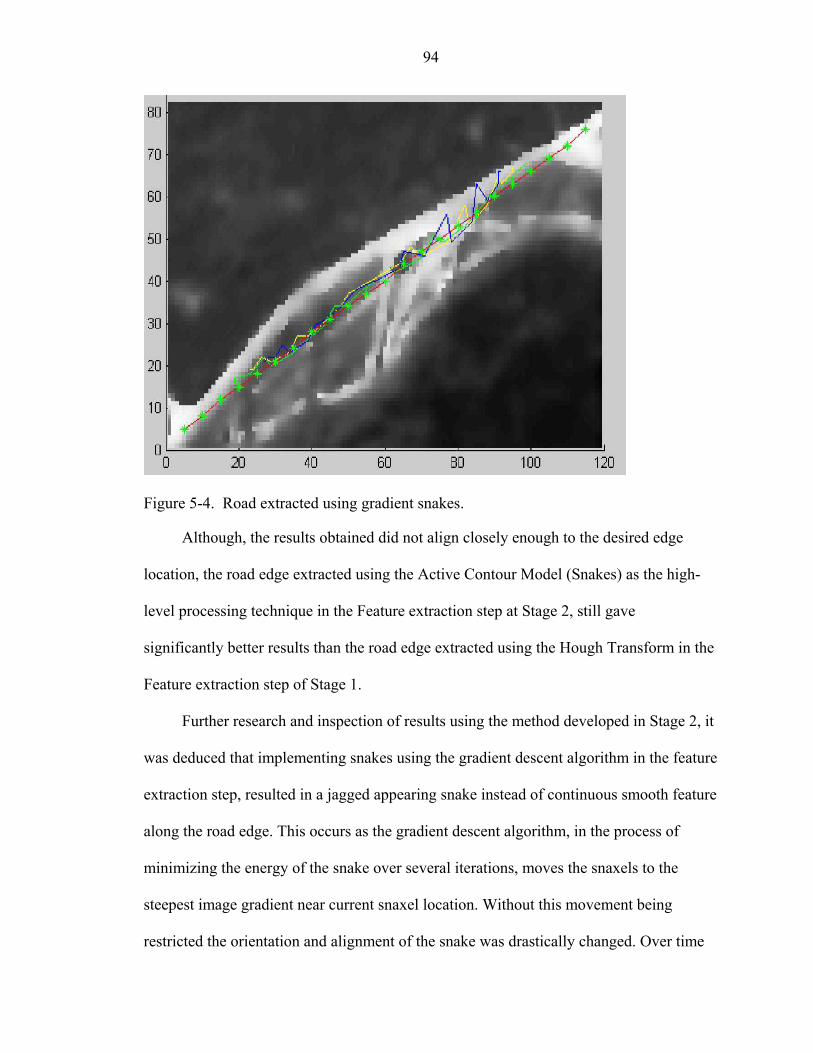
94
Figure 5-4. Road extracted using gradient snakes.
Although, the results obtained did not align closely enough to the desired edge
location, the road edge extracted using the Active Contour Model (Snakes) as the high-
level processing technique in the Feature extraction step at Stage 2, still gave
significantly better results than the road edge extracted using the Hough Transform in the
Feature extraction step of Stage 1.
Further research and inspection of results using the method developed in Stage 2, it
was deduced that implementing snakes using the gradient descent algorithm in the feature
extraction step, resulted in a jagged appearing snake instead of continuous smooth feature
along the road edge. This occurs as the gradient descent algorithm, in the process of
minimizing the energy of the snake over several iterations, moves the snaxels to the
steepest image gradient near current snaxel location. Without this movement being
restricted the orientation and alignment of the snake was drastically changed. Over time
95
steps or iteration, this algorithm significantly affected the alignment of the snake, by
making the snaxels converge to the steepest gradient in the image and moving the snake
away from the desired road edge location.
Problem with aligning the snake to the desired road edge lead to the
implementation of snakes using dynamic programming. This method was developed
during Stage 3 of the development process. The principles and implementation of
dynamic programming for snake energy minimization are explained in detail in Chapter
4.
The results obtained using the method developed in Stage 3 showed the appropriate
aligning of snakes or extracted road edges to the desired road edge location. The roads
extracted at this stage showed better fits when compared to any of the prior stages.
Although some results did get significantly effected by noise or other road edges, with
similar gradients, near the desired road edge; this resulted in major movement of the
snake from the desired road edge locations. The central portion of the road segment
extracted in Figure 5-5 is a good example of such a problem.
Figure 5-5 illustrates a road segment extracted using Gaussian blurring and the
Dynamic Snake, as developed in Stage 3. The extracted road segment, or snake, is
represented in green with final snaxels positions in red. Initial locations of the snaxels are
represented in blue. In Figure 5-5, the extracted road segment is away from the desired
road edge in the central portion of the segment, whereas, toward the ends of the segment,
it aligns closely to the outer edge of the road.
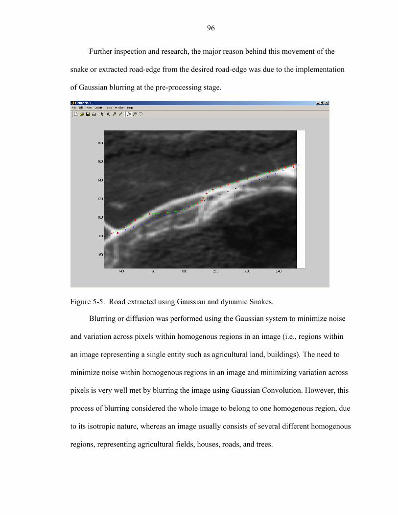
96
Further inspection and research, the major reason behind this movement of the
snake or extracted road-edge from the desired road-edge was due to the implementation
of Gaussian blurring at the pre-processing stage.
Figure 5-5. Road extracted using Gaussian and dynamic Snakes.
Blurring or diffusion was performed using the Gaussian system to minimize noise
and variation across pixels within homogenous regions in an image (i.e., regions within
an image representing a single entity such as agricultural land, buildings). The need to
minimize noise within homogenous regions in an image and minimizing variation across
pixels is very well met by blurring the image using Gaussian Convolution. However, this
process of blurring considered the whole image to belong to one homogenous region, due
to its isotropic nature, whereas an image usually consists of several different homogenous
regions, representing agricultural fields, houses, roads, and trees.
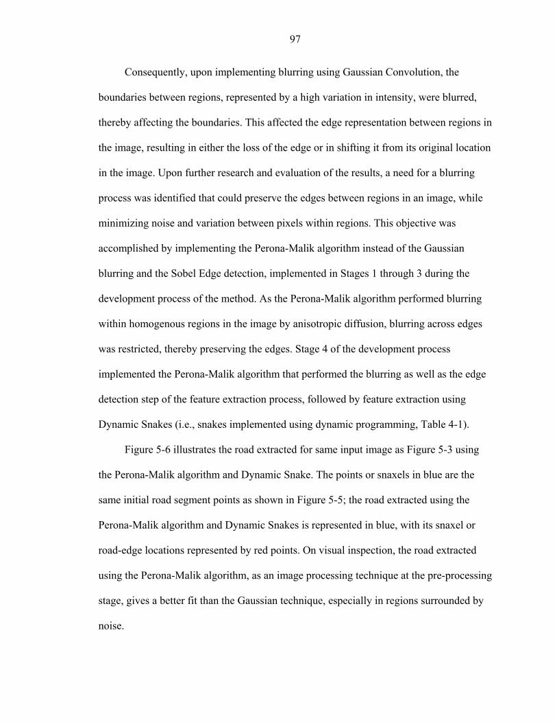
97
Consequently, upon implementing blurring using Gaussian Convolution, the
boundaries between regions, represented by a high variation in intensity, were blurred,
thereby affecting the boundaries. This affected the edge representation between regions in
the image, resulting in either the loss of the edge or in shifting it from its original location
in the image. Upon further research and evaluation of the results, a need for a blurring
process was identified that could preserve the edges between regions in an image, while
minimizing noise and variation between pixels within regions. This objective was
accomplished by implementing the Perona-Malik algorithm instead of the Gaussian
blurring and the Sobel Edge detection, implemented in Stages 1 through 3 during the
development process of the method. As the Perona-Malik algorithm performed blurring
within homogenous regions in the image by anisotropic diffusion, blurring across edges
was restricted, thereby preserving the edges. Stage 4 of the development process
implemented the Perona-Malik algorithm that performed the blurring as well as the edge
detection step of the feature extraction process, followed by feature extraction using
Dynamic Snakes (i.e., snakes implemented using dynamic programming, Table 4-1).
Figure 5-6 illustrates the road extracted for same input image as Figure 5-3 using
the Perona-Malik algorithm and Dynamic Snake. The points or snaxels in blue are the
same initial road segment points as shown in Figure 5-5; the road extracted using the
Perona-Malik algorithm and Dynamic Snakes is represented in blue, with its snaxel or
road-edge locations represented by red points. On visual inspection, the road extracted
using the Perona-Malik algorithm, as an image processing technique at the pre-processing
stage, gives a better fit than the Gaussian technique, especially in regions surrounded by
noise.
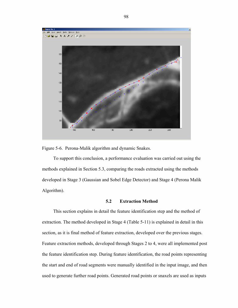
98
Figure 5-6. Perona-Malik algorithm and dynamic Snakes.
To support this conclusion, a performance evaluation was carried out using the
methods explained in Section 5.3, comparing the roads extracted using the methods
developed in Stage 3 (Gaussian and Sobel Edge Detector) and Stage 4 (Perona Malik
Algorithm).
5.2 Extraction Method
This section explains in detail the feature identification step and the method of
extraction. The method developed in Stage 4 (Table 5-11) is explained in detail in this
section, as it is final method of feature extraction, developed over the previous stages.
Feature extraction methods, developed through Stages 2 to 4, were all implemented post
the feature identification step. During feature identification, the road points representing
the start and end of road segments were manually identified in the input image, and then
used to generate further road points. Generated road points or snaxels are used as inputs
99
for the final step of feature extraction in Stages 2 to 4. Hence, road extraction is
initialized by the feature identification step, where a user manually identifies and selects
the start and end of those road segments forming the road network in a given input image.
The coordinates for the start and end of road segments, selected during the feature
identification step, are stored in the process, and are used to further interpolate road
points or snaxels. They represent the initial estimated location of road edges in the image
and the subset road segment image from the pre-processed input image. During the first
step of extraction the input image is pre-processed, or diffused, to minimize noise and
variation within regions in the image. In the method developed in Stage 4, the input
image is pre-processed using the Perona-Malik algorithm that performs both edge
detection and blurring simultaneously, to restrict blurring across edges. Using the road
segment information, road points or snaxels are interpolated for each segment, and a
corresponding road segment image is cropped as a subset of the diffused/blurred image
that was obtained through the pre-processing and edge detection steps. Interpolated road
points, or snaxels, coordinates are transformed to the coordinate system of the road
segment image. The road segment image, along with the transformed snaxel coordinates,
is used as the input for the feature extraction step. The feature extraction step is
implemented using Dynamic Snakes. The resultant road edges, detected through the
feature extraction step, are transformed back to the coordinate system of the input image,
thereby aligning the extracted road to the desired road edge feature.
The image considered for road feature extraction was a DOQQ (Digital Ortho
Quarter Quadrangles) with dimensions of 1000x1000 pixels, obtained from
www.labins.org. This image was converted to a grayscale image of 250x250 image pixel
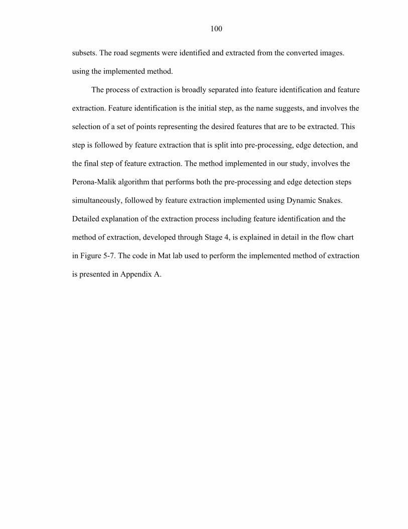
100
subsets. The road segments were identified and extracted from the converted images.
using the implemented method.
The process of extraction is broadly separated into feature identification and feature
extraction. Feature identification is the initial step, as the name suggests, and involves the
selection of a set of points representing the desired features that are to be extracted. This
step is followed by feature extraction that is split into pre-processing, edge detection, and
the final step of feature extraction. The method implemented in our study, involves the
Perona-Malik algorithm that performs both the pre-processing and edge detection steps
simultaneously, followed by feature extraction implemented using Dynamic Snakes.
Detailed explanation of the extraction process including feature identification and the
method of extraction, developed through Stage 4, is explained in detail in the flow chart
in Figure 5-7. The code in Mat lab used to perform the implemented method of extraction
is presented in Appendix A.
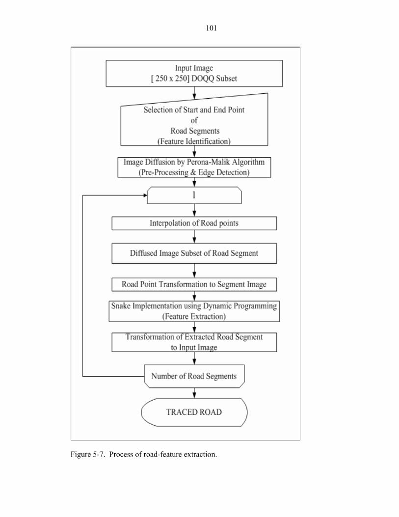
101
Figure 5-7. Process of road-feature extraction.
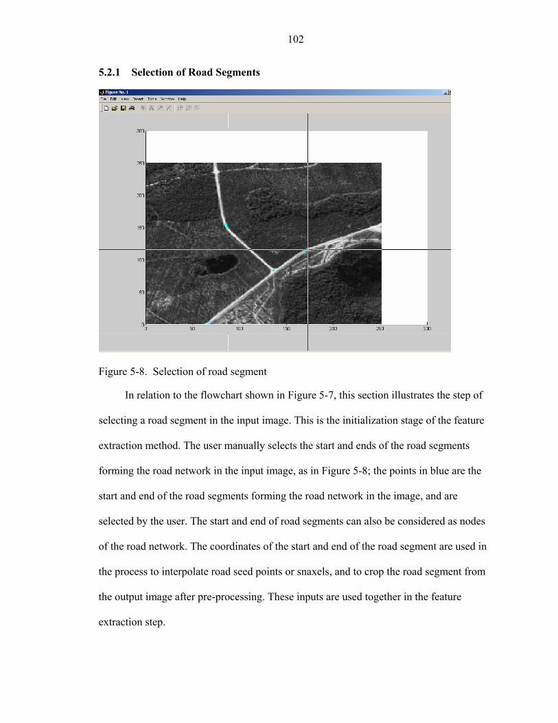
102
5.2.1 Selection of Road Segments
Figure 5-8. Selection of road segment
In relation to the flowchart shown in Figure 5-7, this section illustrates the step of
selecting a road segment in the input image. This is the initialization stage of the feature
extraction method. The user manually selects the start and ends of the road segments
forming the road network in the input image, as in Figure 5-8; the points in blue are the
start and end of the road segments forming the road network in the image, and are
selected by the user. The start and end of road segments can also be considered as nodes
of the road network. The coordinates of the start and end of the road segment are used in
the process to interpolate road seed points or snaxels, and to crop the road segment from
the output image after pre-processing. These inputs are used together in the feature
extraction step.
103
5.2.2 Image Diffusion
Image diffusion, or blurring, is performed as a pre-processing step operation prior
to performing road point interpolation, or generation of snaxels that represent the
estimated road edge locations. As per Stage 4, the Perona-Malik algorithm is
implemented at the pre-processing stage to diffuse the input image instead of Gaussian
blurring, as explained earlier in Section 5.1. The Perona-Malik algorithm blurs the image
based on the principle of anisotropic diffusion. Based on the principle of anisotropic
diffusion, the Perona-Malik algorithm blurs the image based on a predefined criterion; as
compared to Gaussian blurring, using isotropic diffusion that blurs in a similar fashion
across the image. The Perona-Malik algorithm blurs the image with a criterion that is set
to blur only within homogenous regions in an image, and to restrict blurring between
regions, thus preserving the edge information in an image. This ability of the Perona-
Malik algorithm helps to retain the much needed edge information that is used for road
edge extraction later in the process.
Figure 5-9 illustrates the blurring of a highlighted intersection region in the original
image. The insets overlaid on the original image illustrate the blurred portion of the
highlighted intersection in the original image. The inset on the left, highlighted in the red
block, represents the edge between the road and the adjacent region, pre-processed using
the Perona-Malik algorithm, and the inset of the right highlighted in blue represents the
edge between the road and the same adjacent region, pre-processed using the Gaussian
convolution. As can be seen on close inspection, the road edge is better defined in the
anisotropic diffused image, the inset on the left, as compared to the edge highlighted in
blue on the right, blurred using Gaussian that has a jagged appearance.
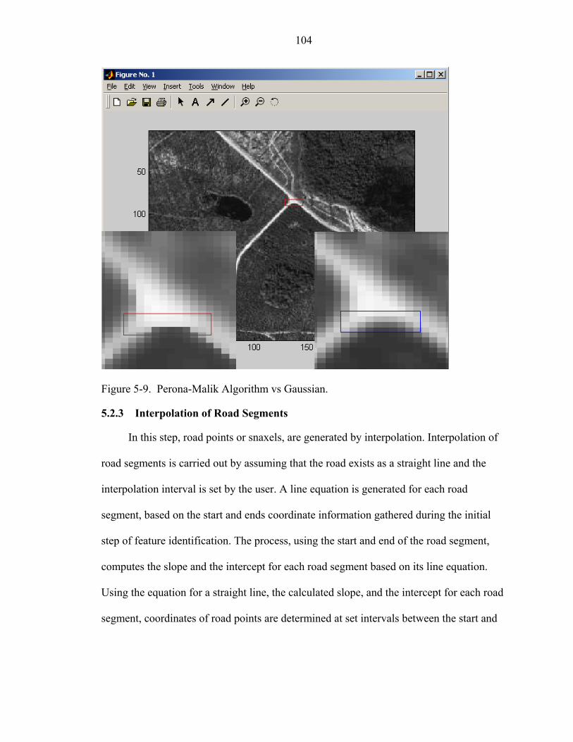
104
Figure 5-9. Perona-Malik Algorithm vs Gaussian.
5.2.3 Interpolation of Road Segments
In this step, road points or snaxels, are generated by interpolation. Interpolation of
road segments is carried out by assuming that the road exists as a straight line and the
interpolation interval is set by the user. A line equation is generated for each road
segment, based on the start and ends coordinate information gathered during the initial
step of feature identification. The process, using the start and end of the road segment,
computes the slope and the intercept for each road segment based on its line equation.
Using the equation for a straight line, the calculated slope, and the intercept for each road
segment, coordinates of road points are determined at set intervals between the start and
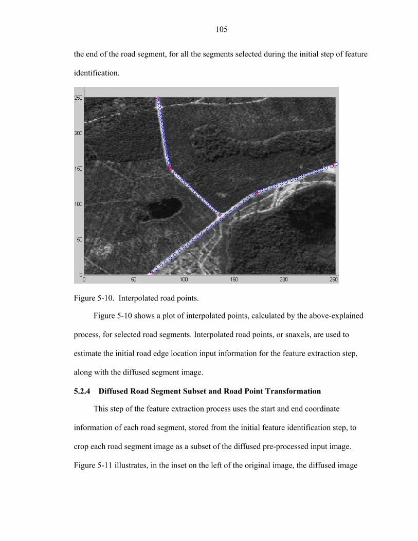
105
the end of the road segment, for all the segments selected during the initial step of feature
identification.
Figure 5-10. Interpolated road points.
Figure 5-10 shows a plot of interpolated points, calculated by the above-explained
process, for selected road segments. Interpolated road points, or snaxels, are used to
estimate the initial road edge location input information for the feature extraction step,
along with the diffused segment image.
5.2.4 Diffused Road Segment Subset and Road Point Transformation
This step of the feature extraction process uses the start and end coordinate
information of each road segment, stored from the initial feature identification step, to
crop each road segment image as a subset of the diffused pre-processed input image.
Figure 5-11 illustrates, in the inset on the left of the original image, the diffused image
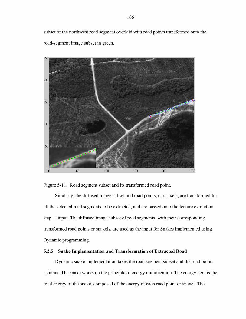
106
subset of the northwest road segment overlaid with road points transformed onto the
road-segment image subset in green.
Figure 5-11. Road segment subset and its transformed road point.
Similarly, the diffused image subset and road points, or snaxels, are transformed for
all the selected road segments to be extracted, and are passed onto the feature extraction
step as input. The diffused image subset of road segments, with their corresponding
transformed road points or snaxels, are used as the input for Snakes implemented using
Dynamic programming.
5.2.5 Snake Implementation and Transformation of Extracted Road
Dynamic snake implementation takes the road segment subset and the road points
as input. The snake works on the principle of energy minimization. The energy here is the
total energy of the snake, composed of the energy of each road point or snaxel. The
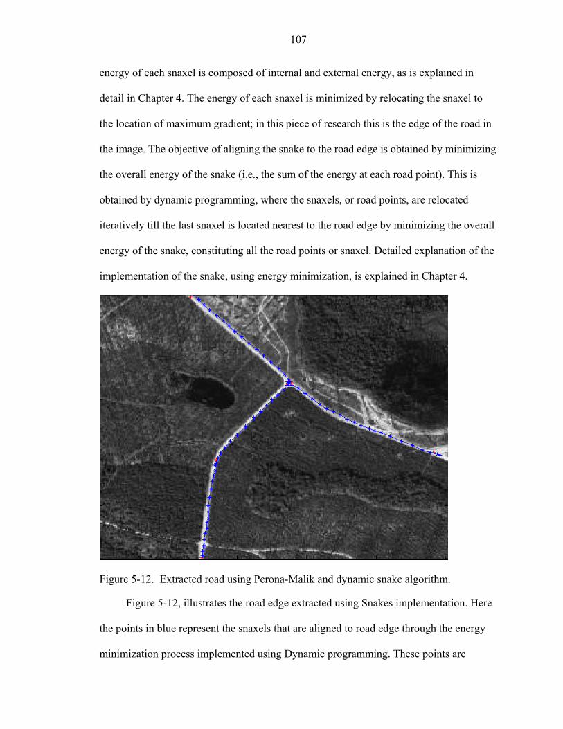
107
energy of each snaxel is composed of internal and external energy, as is explained in
detail in Chapter 4. The energy of each snaxel is minimized by relocating the snaxel to
the location of maximum gradient; in this piece of research this is the edge of the road in
the image. The objective of aligning the snake to the road edge is obtained by minimizing
the overall energy of the snake (i.e., the sum of the energy at each road point). This is
obtained by dynamic programming, where the snaxels, or road points, are relocated
iteratively till the last snaxel is located nearest to the road edge by minimizing the overall
energy of the snake, constituting all the road points or snaxel. Detailed explanation of the
implementation of the snake, using energy minimization, is explained in Chapter 4.
Figure 5-12. Extracted road using Perona-Malik and dynamic snake algorithm.
Figure 5-12, illustrates the road edge extracted using Snakes implementation. Here
the points in blue represent the snaxels that are aligned to road edge through the energy
minimization process implemented using Dynamic programming. These points are
108
further concatenated to form a spline, represented in blue. The red points in Figure 5-12
represent the start and end of the road segments selected at the initial feature
identification step. Section 5.3, speaks more in brief about the method of evaluation used
to support the implemented method, as compared to road edge feature extracted using
Stage 3.
5.3 Evaluation Method
The roads extracted during the first two stages were, on visual inspection,
considered undesirable, as they could not extract the desired road edge locations, as in
Section 5.1. Hence, further stages were developed through experimentation using a
combination of image processing techniques. The results obtained through the methods
developed in Stage 3 and the final stage (i.e., Stage 4) of the development process was
close to the desired road edges in the image. Inspection of the results on a dataset of 10
road segments obtained through implementation of the method developed in Stage 4 gave
better results as compared to the results obtained in Stage 3. To support this conclusion,
an evaluation of the method of extraction was performed, based on the extracted road
edge information from each stage (i.e., Stage 3 and Stage 4), against the road edge
extracted by a manual process.
Performance on road extraction, when implemented using methods developed in
Stage 3 and Stage 4, was determined using goodness of fit and F-test statistics. The mean
squared error was calculated for each road segment extracted, based on the difference
between the coordinates of desired road point, or snaxel, location and the final road point,
or snaxel, location obtained using Stage 3 and Stage 4. Further a hypothesis was
developed based on the performance of the methods developed in Stage 3 and Stage 4
were evaluated. Thus, the criteria for evaluation of the method of extraction were based
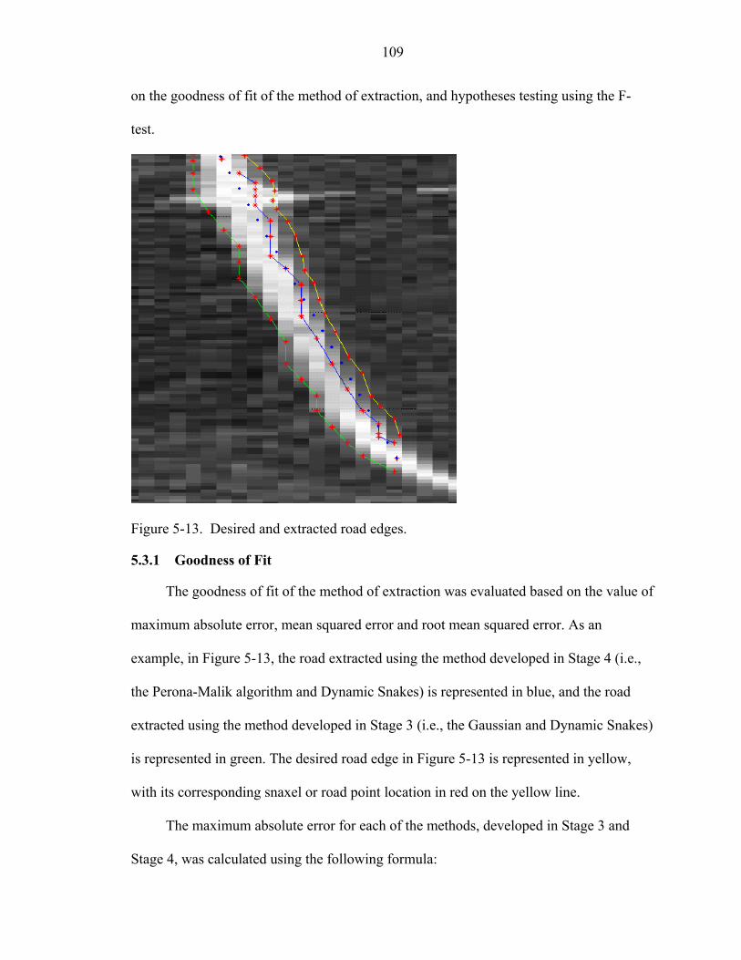
109
on the goodness of fit of the method of extraction, and hypotheses testing using the F-
test.
Figure 5-13. Desired and extracted road edges.
5.3.1 Goodness of Fit
The goodness of fit of the method of extraction was evaluated based on the value of
maximum absolute error, mean squared error and root mean squared error. As an
example, in Figure 5-13, the road extracted using the method developed in Stage 4 (i.e.,
the Perona-Malik algorithm and Dynamic Snakes) is represented in blue, and the road
extracted using the method developed in Stage 3 (i.e., the Gaussian and Dynamic Snakes)
is represented in green. The desired road edge in Figure 5-13 is represented in yellow,
with its corresponding snaxel or road point location in red on the yellow line.
The maximum absolute error for each of the methods, developed in Stage 3 and
Stage 4, was calculated using the following formula:
110
If di = distance between the actual/desired road point or snaxel, and the extracted
road point or snaxel
Where i = 1 to n, and n is the number of snaxels or road point locations.
Then, the maximum absolute error = maxi | di |
With respect to Figure 5-13, the distance between the desired snaxel location (red
dots on the yellow road edge in Figure 5-13) and their corresponding snaxel positions
obtained through the methods implemented in Stage 3 (red dots on green in Figure 5-13)
and Stage 4 (red dots on blue in Figure 5-13) were calculated. From the calculated
differences between the desired snaxel positions and extracted snaxel positions, the one
with the maximum value in each of the methods gave an estimate of how far a snaxel in
each method could deviate from its desired location, also known as the maximum
absolute error. Furthermore, an overall measure of the deviation of the curve, or extracted
road edge, from the desired road edge was determined from the mean squared error. This
value was calculated by determining the mean of the squares of the difference, or
distance of each extracted snaxel from its corresponding desired location.
Mean Squared Error = 2
1/1 ∑ =
n
iidn
The square root of mean squared error was used as a performance indicator on the
extraction process. The lower the root mean squared error, the better the method of
extraction. Furthermore, the mean squared error value calculated in this method of
evaluation was also used in the generation of a hypothesis for the F-test.
5.3.2 F-Test
An F-test was performed by generating a hypothesis based on the comparison of
mean squared values for the roads extracted using the methods developed in Stage 3 and
111
Stage 4. This test was performed on road segments extracted from a set of test data of 10
road segment image subsets based on the following Null hypotheses.
H0 : Mean Squared Error Anisotropic = Mean Squared Error Gaussian
HA : Mean Squared Error Anisotropic < Mean Squared Error Gaussian
HG : Mean Squared Error Anisotropic > Mean Squared Error Gaussian
Where:
Mean Squared Error Anisotropic = Mean Squared Error for the road extracted
using the method developed using the Perona-Malik Algorithm and Dynamic Snakes
implemented in Stage 4.
Mean Squared Error Gaussian = Mean Squared Error for the road extracted using
the method developed using the Gaussian blurring and Dynamic Snakes implemented in
Stage 3.
If
H0 = True, resulted in similar performance by both methods,
HA = True, resulted in Anisotropic Diffusion (Stage 4) performing better when
compared to Gaussian (Stage 3).
HG = True, resulted in Gaussian (Stage 3) performing better when compared to
Anisotropic Diffusion (Stage 4).
Further, evaluation was carried out on a set of 10 image subsets that were extracted
using Stage 3 and Stage 4, using goodness of fit and the F-test. Chapter 6, illustrates the
results obtained using the methods developed in Stage 3 and Stage 4, followed by an
evaluation and analysis of the results obtained.
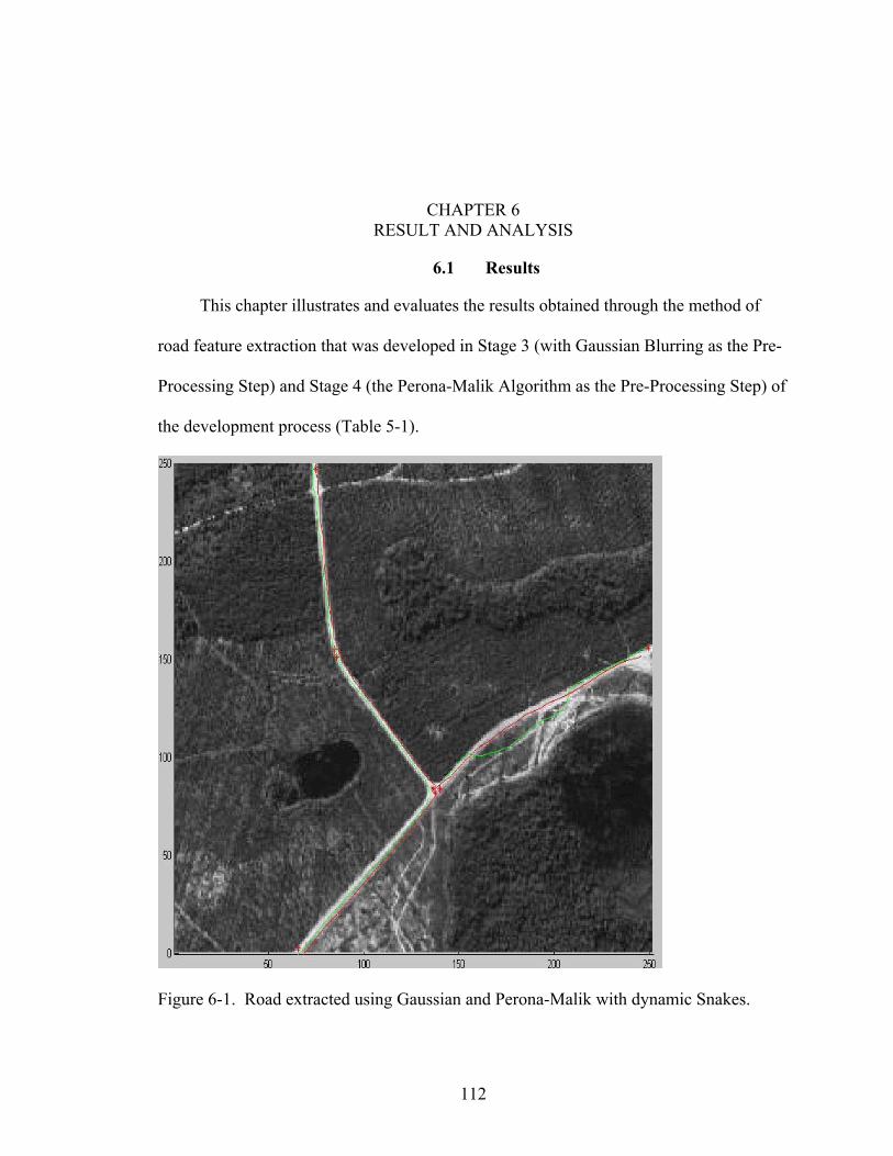
112
CHAPTER 6 RESULT AND ANALYSIS
6.1 Results
This chapter illustrates and evaluates the results obtained through the method of
road feature extraction that was developed in Stage 3 (with Gaussian Blurring as the Pre-
Processing Step) and Stage 4 (the Perona-Malik Algorithm as the Pre-Processing Step) of
the development process (Table 5-1).
Figure 6-1. Road extracted using Gaussian and Perona-Malik with dynamic Snakes.
113
Figure 6-1, illustrates a final extracted road, using the method from Stage 3 for the
green line (Gaussian) and the method from Stage 4 for the red (Perona-Malik Algorithm).
The methods of extraction developed in Stage 3 and Stage 4, were similar except for the
initial pre-processing step. In Stage 3, the initial pre-processing was implemented using
Gaussian, an isotropic diffusion technique, and in Stage 4, it was implemented using the
Perona-Malik Algorithm, an anisotropic diffusion technique.
6.2 Analysis of Result on Test Images
The performance of the methods of extraction, developed in Stage 3 and Stage 4, is
to be evaluated from their implementation on a set of 10 road segments. The performance
of Stage 3 (Gaussian) and Stage 4 (Perona-Malik Algorithm) is determined by evaluating
the goodness of fit and the F-test statistic for each extracted road segment. The method of
evaluation using goodness of fit and the F-test is explained in detail in Section 5.3.
Goodness of fit was determined for each extracted road segment, and gives basic
statistical evidence concerning how well the road is extracted using each method of
extraction, based on the following factors:
• Maximum absolute error: This value gives a numerical description of how far (in pixels) an extracted edge (snaxel or road edge) is from the actual/desired road edge in an image.
• Mean Squared Error: This gives a numerical description of how well the overall Snake or extracted road is aligned to the desired road edge. The square root of the mean squared error is used as a performance indicator, where lower values of the root mean square suggest better performance from that method of extraction.
An F-test statistic was also performed to compare the methods of extraction that
were implemented on each road segment, to evaluate the best method of extraction. This
test was based on a hypothesis developed using the mean squared error value that was
114
calculated for each road segment from the evaluated goodness of fit, as was explained in
Section 5.3.
Figure 6-2 (A to J) illustrate the road segment images and their extracted output.
The roads extracted using Gaussian as pre-processing step (Stage 3) are represented in
green, and roads extracted using the Perona-Malik algorithm as the pre-processing step
(Stage 4) are represented in blue. Green dots along green lines in the image represent the
final snaxel, or road edge, positions after Stage 3 implementation; blue dots along blue
lines represent the final snaxel, or road edge, positions after Stage 4 implementation.
On visual inspection of the roads extracted, the method implemented in Stage 4
(Perona-Malik algorithm) performed better than the one implemented in Stage 3
(Gaussian). Thus to support this evaluation, goodness of fit and an F-test, as per the
hypothesis explained in Section 5.3, were performed on each of 10 images in Figure 6-
2(A-J). The final location of the snaxels, or road edge points, green and blue in color for
Stages 3 and 4 respectively, were determined and compared to their desired location that
was specified by the user on the image. The distance between the desired and the actual
location gave an absolute error for each edge position extracted. A maximum absolute
error was determined for each road extracted, giving a numerical estimate of the
maximum extent to which an extracted edge deviated, in the implemented method of
extraction.
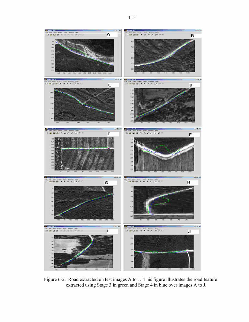
115
Figure 6-2. Road extracted on test images A to J. This figure illustrates the road feature
extracted using Stage 3 in green and Stage 4 in blue over images A to J.
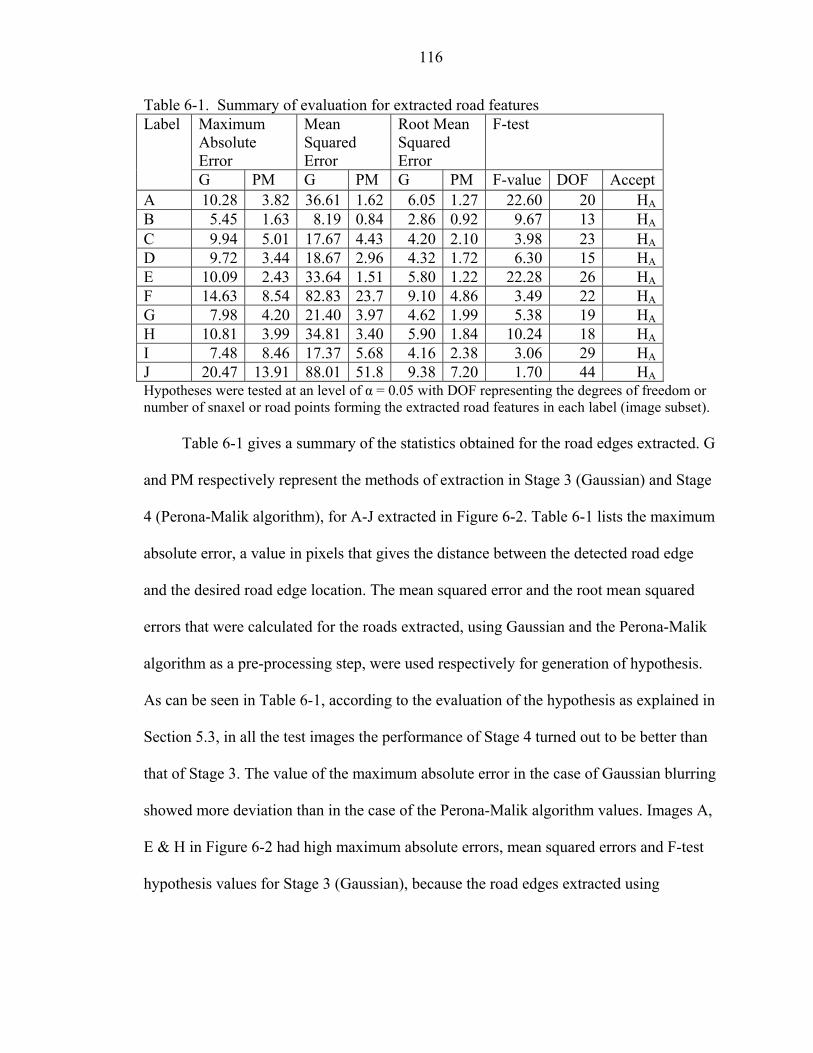
116
Table 6-1. Summary of evaluation for extracted road features Maximum Absolute Error
Mean Squared Error
Root Mean Squared Error
F-test
Label
G PM G PM G PM F-value DOF AcceptA 10.28 3.82 36.61 1.62 6.05 1.27 22.60 20 HAB 5.45 1.63 8.19 0.84 2.86 0.92 9.67 13 HA
C 9.94 5.01 17.67 4.43 4.20 2.10 3.98 23 HAD 9.72 3.44 18.67 2.96 4.32 1.72 6.30 15 HAE 10.09 2.43 33.64 1.51 5.80 1.22 22.28 26 HAF 14.63 8.54 82.83 23.7 9.10 4.86 3.49 22 HAG 7.98 4.20 21.40 3.97 4.62 1.99 5.38 19 HAH 10.81 3.99 34.81 3.40 5.90 1.84 10.24 18 HAI 7.48 8.46 17.37 5.68 4.16 2.38 3.06 29 HAJ 20.47 13.91 88.01 51.8 9.38 7.20 1.70 44 HAHypotheses were tested at an level of α = 0.05 with DOF representing the degrees of freedom or number of snaxel or road points forming the extracted road features in each label (image subset).
Table 6-1 gives a summary of the statistics obtained for the road edges extracted. G
and PM respectively represent the methods of extraction in Stage 3 (Gaussian) and Stage
4 (Perona-Malik algorithm), for A-J extracted in Figure 6-2. Table 6-1 lists the maximum
absolute error, a value in pixels that gives the distance between the detected road edge
and the desired road edge location. The mean squared error and the root mean squared
errors that were calculated for the roads extracted, using Gaussian and the Perona-Malik
algorithm as a pre-processing step, were used respectively for generation of hypothesis.
As can be seen in Table 6-1, according to the evaluation of the hypothesis as explained in
Section 5.3, in all the test images the performance of Stage 4 turned out to be better than
that of Stage 3. The value of the maximum absolute error in the case of Gaussian blurring
showed more deviation than in the case of the Perona-Malik algorithm values. Images A,
E & H in Figure 6-2 had high maximum absolute errors, mean squared errors and F-test
hypothesis values for Stage 3 (Gaussian), because the road edges extracted using
117
Gaussian deviated drastically from the desired road edge, as can be seen in the results
obtained in images A, E, H (Figure 6-2).
Thus on visual interpretation of the results in images A, E, H ( Figure 6-2)., along
with the basic statistics and hypothesis evaluation presented in Table 6-1, the method
from Stage 4 performed much better than the method of extraction developed in Stage 3.
Hence, the method of extraction developed using a combination of the Perona-Malik
algorithm, an anisotropic diffusion pre-processing approach, along with Snakes,
implemented using dynamic programming, gives the best result when compared to any
other combination of techniques tested through Stages 1 to 4, as listed in Section 5.1.
118
CHAPTER 7 CONCLUSION AND FUTURE WORK
7.1 Conclusion
In our study, the road-extraction methods that were developed in stages, were
compared in Chapter 5, and based on the evaluation in Chapter 6, the method of
extraction developed using the Perona-Malik algorithm and Dynamic Snakes in Stage 4
gave the best results. The test images that were used to evaluate the method of extraction
were made available from land and boundary information system (Source:
http://data.labins.org last accessed: 16 August 2004). The implementation of the Perona-
Malik algorithm in pre-processing and Snakes using dynamic programming at the feature
extraction step (Section 5.1) was significant in getting the desired result. This was due to
blurring of homogenous regions within an image while restricting blurring between
regions within an image. Perona-Malik algorithm therefore led to well defined boundary
information. In comparison, Gaussian blurring, an isotropic blurring technique, blurred
the image uniformly, led to shifts in boundaries, or incomplete boundary information.
Thus, pre-processing using the Perona-Malik algorithm performed better than
conventional Gaussian blurring.
In addition to the Perona-Malik algorithm, implementing Snakes (Active Contour
Models) lead to the extraction of the appropriate road edges, whereas implementation of
the Hough Transform that performed a general straight-line feature extraction within an
input image, failed to do so (Section 5.1). Above all, the results using Snakes were
enhanced when implemented using Dynamic programming, rather than the Gradient
119
descent algorithm; this is because of the ability of Dynamic programming to restrict the
movement of the Snake, as was explained in detail in Chapter 4 (Section 5.1).
The method of extraction developed in this research, and the proposals for future
work aimed at automating the initial step of the identification and selection of road
segment points (Section 5.2), may only work on high-resolution images. As, these
processes need edge information for extraction, and geometric (width) and radiometric
(radiometric/intensity variation) characteristic information across the road along the
direction of road, to identify and select road segment points. This information may exist
only in high-resolution images, where roads exist as long continuous features with
uniform width; in the case of low-resolution images, roads exist as long bright lines that
may disappear or exist as very thin features after the pre-processing step. Thus the
method of extraction developed here, and the proposed future work, may not work with
information obtained from low-resolution images. Section 7.2 gives an overview of
future work to be carried out to automate the initial step of identification and selection of
road segments; the suggestion is based on a concept developed by Vosselman and de
Knecht (1995) using the Kalman Filter and Profile Matching approach.
7.2 Future Work
As part of future work in this area, the proposal is to automate the initial step of
identification and selection of the start and end of road segments. To do this the use of
profile matching and the Kalman filter approach (Vosselman and Knecht, 1995) should
be used to identify and select road segments. This process would use an initial model of
the road segment, selected by the user from the input image that is updated on a regular
basis using the Kalman Filter. Appendix B, explains the identification and extraction of

120
road segments using Profile Matching and Kalman Filtering (Vosselman and de Knecht,
1995), this preceded by a Kalman filter principle tutorial (Simon, 2001).
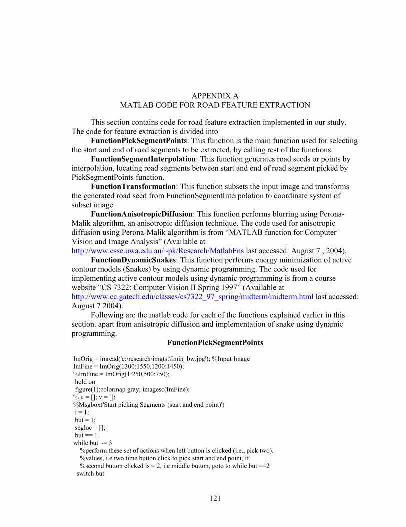
121
APPENDIX A MATLAB CODE FOR ROAD FEATURE EXTRACTION
This section contains code for road feature extraction implemented in our study. The code for feature extraction is divided into
FunctionPickSegmentPoints: This function is the main function used for selecting the start and end of road segments to be extracted, by calling rest of the functions.
FunctionSegmentInterpolation: This function generates road seeds or points by interpolation, locating road segments between start and end of road segment picked by PickSegmentPoints function.
FunctionTransformation: This function subsets the input image and transforms the generated road seed from FunctionSegmentInterpolation to coordinate system of subset image.
FunctionAnisotropicDiffusion: This function performs blurring using Perona-Malik algorithm, an anisotropic diffusion technique. The code used for anisotropic diffusion using Perona-Malik algorithm is from “MATLAB function for Computer Vision and Image Analysis” (Available at http://www.csse.uwa.edu.au/~pk/Research/MatlabFns last accessed: August 7 , 2004).
FunctionDynamicSnakes: This function performs energy minimization of active contour models (Snakes) by using dynamic programming. The code used for implementing active contour models using dynamic programming is from a course website “CS 7322: Computer Vision II Spring 1997” (Available at http://www.cc.gatech.edu/classes/cs7322_97_spring/midterm/midterm.html last accessed: August 7 2004).
Following are the matlab code for each of the functions explained earlier in this section. apart from anisotropic diffusion and implementation of snake using dynamic programming.
FunctionPickSegmentPoints
ImOrig = imread('c:\research\imgtst\Imin_bw.jpg'); %Input Image ImFine = ImOrig(1300:1550,1200:1450); %ImFine = ImOrig(1:250,500:750); hold on figure(1);colormap gray; imagesc(ImFine); % u = []; v = []; %Msgbox('Start picking Segments (start and end point)') i = 1; but = 1; segloc = []; but == 1 while but ~= 3 %perform these set of actions when left button is clicked (i.e., pick two). %values, i.e two time button click to pick start and end point, if %second button clicked is = 2, i.e middle button, goto to while but ==2 switch but
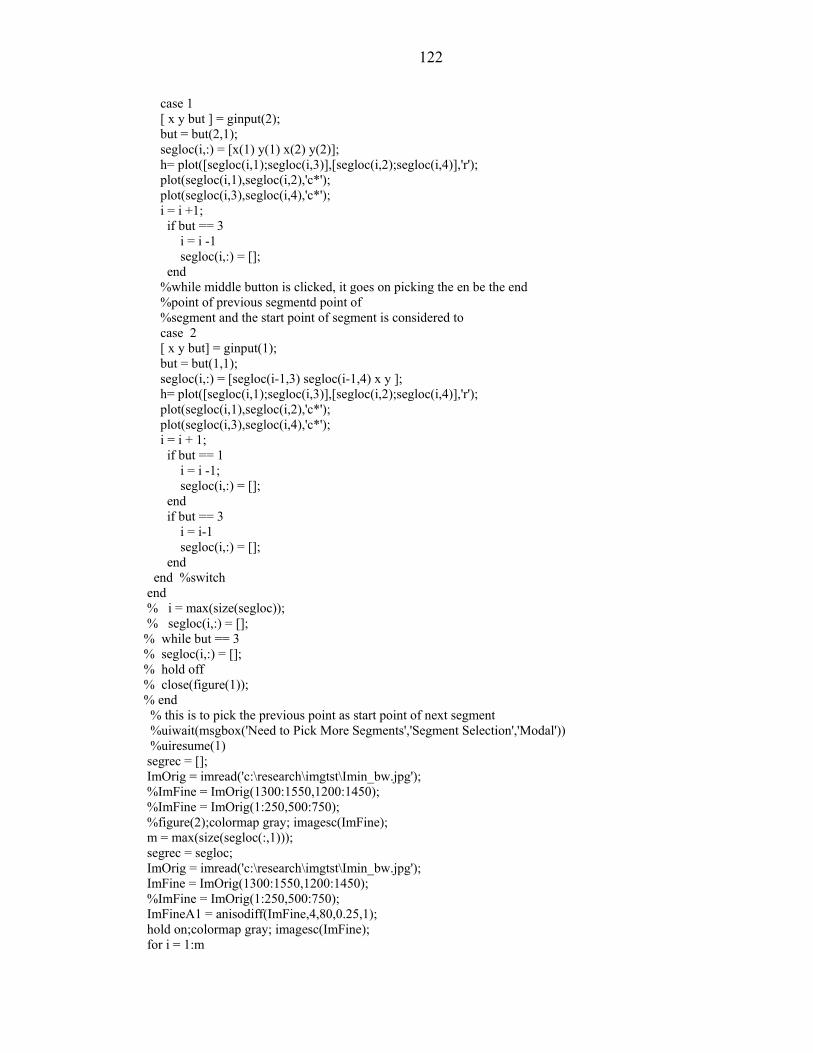
122
case 1 [ x y but ] = ginput(2); but = but(2,1); segloc(i,:) = [x(1) y(1) x(2) y(2)]; h= plot([segloc(i,1);segloc(i,3)],[segloc(i,2);segloc(i,4)],'r'); plot(segloc(i,1),segloc(i,2),'c*'); plot(segloc(i,3),segloc(i,4),'c*'); i = i +1; if but == 3 i = i -1 segloc(i,:) = []; end %while middle button is clicked, it goes on picking the en be the end %point of previous segmentd point of %segment and the start point of segment is considered to case 2 [ x y but] = ginput(1); but = but(1,1); segloc(i,:) = [segloc(i-1,3) segloc(i-1,4) x y ]; h= plot([segloc(i,1);segloc(i,3)],[segloc(i,2);segloc(i,4)],'r'); plot(segloc(i,1),segloc(i,2),'c*'); plot(segloc(i,3),segloc(i,4),'c*'); i = i + 1; if but == 1 i = i -1; segloc(i,:) = []; end if but == 3 i = i-1 segloc(i,:) = []; end end %switch end % i = max(size(segloc)); % segloc(i,:) = []; % while but == 3 % segloc(i,:) = []; % hold off % close(figure(1)); % end % this is to pick the previous point as start point of next segment %uiwait(msgbox('Need to Pick More Segments','Segment Selection','Modal')) %uiresume(1) segrec = []; ImOrig = imread('c:\research\imgtst\Imin_bw.jpg'); %ImFine = ImOrig(1300:1550,1200:1450); %ImFine = ImOrig(1:250,500:750); %figure(2);colormap gray; imagesc(ImFine); m = max(size(segloc(:,1))); segrec = segloc; ImOrig = imread('c:\research\imgtst\Imin_bw.jpg'); ImFine = ImOrig(1300:1550,1200:1450); %ImFine = ImOrig(1:250,500:750); ImFineA1 = anisodiff(ImFine,4,80,0.25,1); hold on;colormap gray; imagesc(ImFine); for i = 1:m
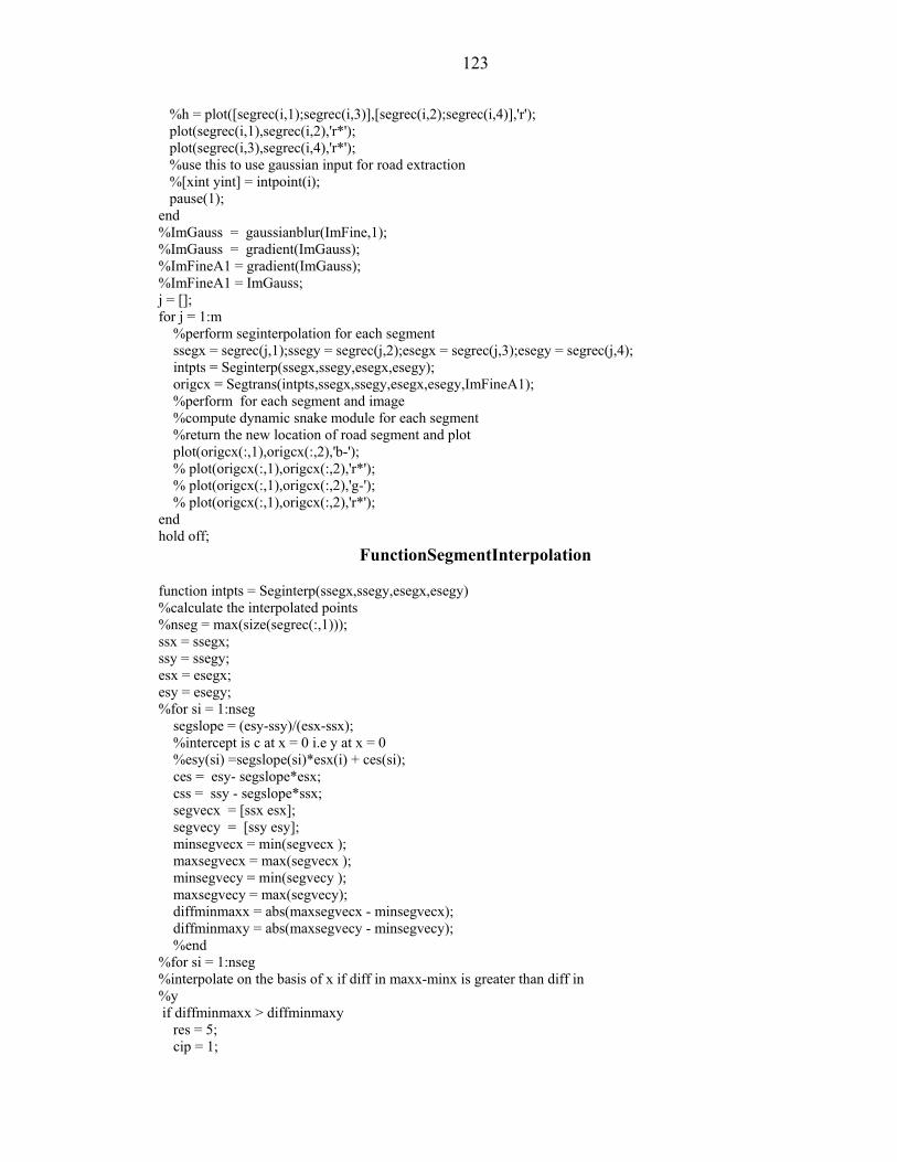
123
%h = plot([segrec(i,1);segrec(i,3)],[segrec(i,2);segrec(i,4)],'r'); plot(segrec(i,1),segrec(i,2),'r*'); plot(segrec(i,3),segrec(i,4),'r*'); %use this to use gaussian input for road extraction %[xint yint] = intpoint(i); pause(1); end %ImGauss = gaussianblur(ImFine,1); %ImGauss = gradient(ImGauss); %ImFineA1 = gradient(ImGauss); %ImFineA1 = ImGauss; j = []; for j = 1:m %perform seginterpolation for each segment ssegx = segrec(j,1);ssegy = segrec(j,2);esegx = segrec(j,3);esegy = segrec(j,4); intpts = Seginterp(ssegx,ssegy,esegx,esegy); origcx = Segtrans(intpts,ssegx,ssegy,esegx,esegy,ImFineA1); %perform for each segment and image %compute dynamic snake module for each segment %return the new location of road segment and plot plot(origcx(:,1),origcx(:,2),'b-'); % plot(origcx(:,1),origcx(:,2),'r*'); % plot(origcx(:,1),origcx(:,2),'g-'); % plot(origcx(:,1),origcx(:,2),'r*'); end hold off;
FunctionSegmentInterpolation
function intpts = Seginterp(ssegx,ssegy,esegx,esegy) %calculate the interpolated points %nseg = max(size(segrec(:,1))); ssx = ssegx; ssy = ssegy; esx = esegx; esy = esegy; %for si = 1:nseg segslope = (esy-ssy)/(esx-ssx); %intercept is c at x = 0 i.e y at x = 0 %esy(si) =segslope(si)*esx(i) + ces(si); ces = esy- segslope*esx; css = ssy - segslope*ssx; segvecx = [ssx esx]; segvecy = [ssy esy]; minsegvecx = min(segvecx ); maxsegvecx = max(segvecx ); minsegvecy = min(segvecy ); maxsegvecy = max(segvecy); diffminmaxx = abs(maxsegvecx - minsegvecx); diffminmaxy = abs(maxsegvecy - minsegvecy); %end %for si = 1:nseg %interpolate on the basis of x if diff in maxx-minx is greater than diff in %y if diffminmaxx > diffminmaxy res = 5; cip = 1;
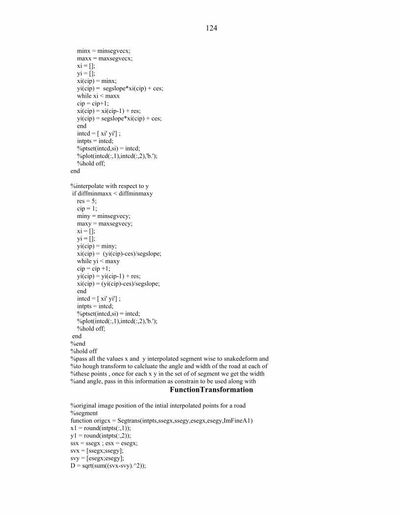
124
minx = minsegvecx; maxx = maxsegvecx; xi = []; yi = []; xi(cip) = minx; yi(cip) = segslope*xi(cip) + ces; while xi < maxx cip = cip+1; xi(cip) = xi(cip-1) + res; yi(cip) = segslope*xi(cip) + ces; end intcd = [ xi' yi'] ; intpts = intcd; %ptset(intcd,si) = intcd; %plot(intcd(:,1),intcd(:,2),'b.'); %hold off; end %interpolate with respect to y if diffminmaxx < diffminmaxy res = 5; cip = 1; miny = minsegvecy; maxy = maxsegvecy; xi = []; yi = []; yi(cip) = miny; xi(cip) = (yi(cip)-ces)/segslope; while yi < maxy cip = cip +1; yi(cip) = yi(cip-1) + res; xi(cip) = (yi(cip)-ces)/segslope; end intcd = [ xi' yi'] ; intpts = intcd; %ptset(intcd,si) = intcd; %plot(intcd(:,1),intcd(:,2),'b.'); %hold off; end %end %hold off %pass all the values x and y interpolated segment wise to snakedeform and %to hough transform to calcluate the angle and width of the road at each of %these points , once for each x y in the set of of segment we get the width %and angle, pass in this information as constrain to be used along with
FunctionTransformation
%original image position of the intial interpolated points for a road %segment function origcx = Segtrans(intpts,ssegx,ssegy,esegx,esegy,ImFineA1) x1 = round(intpts(:,1)); y1 = round(intpts(:,2)); ssx = ssegx ; esx = esegx; svx = [ssegx;ssegy]; svy = [esegx;esegy]; D = sqrt(sum((svx-svy).^2));
125
minx = round(min([ssegx,esegx]))-5; maxx = round(max([ssegx,esegx]))+5; miny = round(min([ssegy,esegy]))-5; maxy = round(max([ssegy,esegy]))+5; cwwidth = round(maxx- minx); cwheight = round(maxy-miny); %anisotropic diffused images = gaussian blurred image. SegIm = imcrop(ImFineA1,[minx,miny,cwwidth,cwheight]); %hold on; %colormap gray;imagesc(SegIm); %interpolated set of snake points. SegImOrig = round(intpts); tx = minx.* ones(size(SegImOrig(:,1))); ty = miny.*ones(size(SegImOrig(:,2))); SegImP = [ SegImOrig(:,1) - tx SegImOrig(:,2) - ty]; SegImPx = SegImP(:,1); SegImPy = SegImP(:,2); %plot(SegImP(:,1),SegImP(:,2),'r-'); %plot(SegImP(:,1),SegImP(:,2),'g*'); [snake_pnts e] = roadsnake(SegImP,SegIm); origcx = [snake_pnts(:,1) + tx , snake_pnts(:,2) + ty]; %newsnakeseg
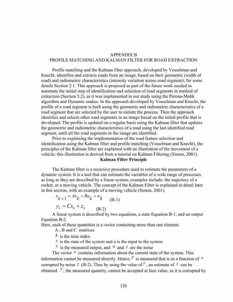
126
APPENDIX B PROFILE MATCHING AND KALMAN FILTER FOR ROAD EXTRACTION
Profile matching and the Kalman filter approach, developed by Vosselman and Knecht, identifies and extracts roads from an image, based on their geometric (width of road) and radiometric characteristics (intensity variation across road segment); for some details Section 2.1. This approach is proposed as part of the future work needed to automate the initial step of identification and selection of road segments in method of extraction (Section 5.2), as it was implemented in our study using the Perona-Malik algorithm and Dynamic snakes. In the approach developed by Vosselman and Knecht, the profile of a road segment is built using the geometric and radiometric characteristics of a road segment that are selected by the user to initiate the process. Then the approach identifies and selects other road segments in an image based on the initial profile that is developed. The profile is updated on a regular basis using the Kalman filter that updates the geometric and radiometric characteristics of a road using the last identified road segment, until all the road segments in the image are identified.
Prior to explaining the implementation of the road feature selection and identification using the Kalman filter and profile matching (Vosselman and Knecht), the principles of the Kalman filter are explained with an illustration of the movement of a vehicle; this illustration is derived from a tutorial on Kalman Filtering (Simon, 2001).
Kalman Filter Principle
The Kalman filter is a recursive procedure used to estimate the parameters of a dynamic system. It is a tool that can estimate the variables of a wide range of processes, as long as they are described by a linear system; examples include: the trajectory of a rocket, or a moving vehicle. The concept of the Kalman Filter is explained in detail later in this section, with an example of a moving vehicle (Simon, 2001).
kwkBukAxkx ++=+1 (B-1)
kkk zCxy += (B-2) A linear system is described by two equations, a state Equation B-1, and an output
Equation B-2. Here, each of these quantities is a vector containing more than one element. A , B and C matrices k is the time index x is the state of the system and u is the input to the system y is the measured output, and w and z are the noise
The vector x contains information about the current state of the system. This information cannot be measured directly. Hence, y is measured that is as a function of x corrupted by noise z (B-2). Thus by using the value of y , an estimate of x can be obtained. y , the measured quantity, cannot be accepted at face value, as it is corrupted by
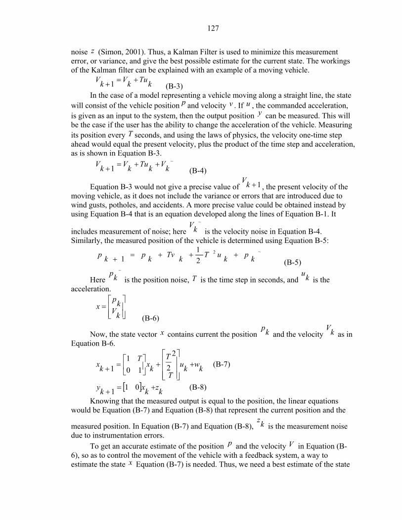
127
noise z (Simon, 2001). Thus, a Kalman Filter is used to minimize this measurement error, or variance, and give the best possible estimate for the current state. The workings of the Kalman filter can be explained with an example of a moving vehicle.
kTukVkV +=+1 (B-3) In the case of a model representing a vehicle moving along a straight line, the state
will consist of the vehicle position p and velocity v . If u , the commanded acceleration, is given as an input to the system, then the output position y can be measured. This will be the case if the user has the ability to change the acceleration of the vehicle. Measuring its position every T seconds, and using the laws of physics, the velocity one-time step ahead would equal the present velocity, plus the product of the time step and acceleration, as is shown in Equation B-3.
~
1 kVkTukVkV ++=+ (B-4)
Equation B-3 would not give a precise value of 1+kV, the present velocity of the
moving vehicle, as it does not include the variance or errors that are introduced due to wind gusts, potholes, and accidents. A more precise value could be obtained instead by using Equation B-4 that is an equation developed along the lines of Equation B-1. It
includes measurement of noise; here ~
kV is the velocity noise in Equation B-4.
Similarly, the measured position of the vehicle is determined using Equation B-5:
~2
21
1 kpkuTkTvkpkp +++=+ (B-5)
Here ~
kp is the position noise, T is the time step in seconds, and ku
is the acceleration.
=
kVkp
x (B-6)
Now, the state vector x contains current the position kp and the velocity kV
as in Equation B-6.
kwkuT
Tkx
Tkx +
+
=+
2
2101
1 (B-7)
[ ] kzkxky +=+ 011 (B-8)
Knowing that the measured output is equal to the position, the linear equations would be Equation (B-7) and Equation (B-8) that represent the current position and the
measured position. In Equation (B-7) and Equation (B-8), kz is the measurement noise
due to instrumentation errors. To get an accurate estimate of the position p and the velocity V in Equation (B-
6), so as to control the movement of the vehicle with a feedback system, a way to estimate the state x Equation (B-7) is needed. Thus, we need a best estimate of the state
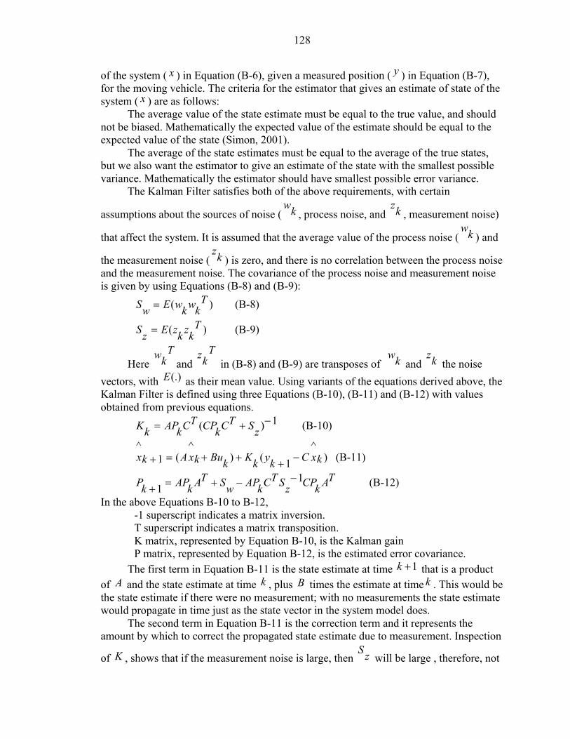
128
of the system ( x ) in Equation (B-6), given a measured position ( y ) in Equation (B-7), for the moving vehicle. The criteria for the estimator that gives an estimate of state of the system ( x ) are as follows:
The average value of the state estimate must be equal to the true value, and should not be biased. Mathematically the expected value of the estimate should be equal to the expected value of the state (Simon, 2001).
The average of the state estimates must be equal to the average of the true states, but we also want the estimator to give an estimate of the state with the smallest possible variance. Mathematically the estimator should have smallest possible error variance.
The Kalman Filter satisfies both of the above requirements, with certain
assumptions about the sources of noise ( kw, process noise, and kz
, measurement noise)
that affect the system. It is assumed that the average value of the process noise ( kw) and
the measurement noise ( kz) is zero, and there is no correlation between the process noise
and the measurement noise. The covariance of the process noise and measurement noise is given by using Equations (B-8) and (B-9): )( T
kwkwEwS = (B-8)
)( TkzkzEzS = (B-9)
Here T
kwand
Tkz
in (B-8) and (B-9) are transposes of kw and kz
the noise vectors, with (.)E as their mean value. Using variants of the equations derived above, the Kalman Filter is defined using three Equations (B-10), (B-11) and (B-12) with values obtained from previous equations.
1)( −+= zSTCkCPTCkAPkK (B-10)
)^
1()^
(1^
kxCkykKkBukxAkx −+++=+ (B-11)
TAkCPzSTCkAPwSTAkAPkP 11
−−+=+ (B-12)
In the above Equations B-10 to B-12, -1 superscript indicates a matrix inversion. T superscript indicates a matrix transposition. K matrix, represented by Equation B-10, is the Kalman gain P matrix, represented by Equation B-12, is the estimated error covariance.
The first term in Equation B-11 is the state estimate at time 1+k that is a product of A and the state estimate at time k , plus B times the estimate at time k . This would be the state estimate if there were no measurement; with no measurements the state estimate would propagate in time just as the state vector in the system model does.
The second term in Equation B-11 is the correction term and it represents the amount by which to correct the propagated state estimate due to measurement. Inspection
of K , shows that if the measurement noise is large, then zS will be large , therefore, not
129
much credibility would be assigned to a measurement of y in computing the next state
estimate ^x ; on the other hand if the measurement noise is small, zS
will be small, so K will be thereby give a lot of credibility to the measurement y , while it is used in
computing the next state estimate ^x . Thus using the set of Kalman Filter equations, the
next state estimates can be found for a moving vehicle. The next section discusses in detail the process of road tracing, using profile matching and Kalman Filtering, as was developed by Vosselman and Knecht.
Road Tracing Using Kalman Filter and Profile Matching
Vosselman and de Knecht (1995) developed a road tracing technique using profile matching and the Kalman Filter technique. In this method, an operator initializes a road tracer by placing two points that indicate a short road segment. Between these two points, grey value cross sections are computed at intervals of one pixel. The model profile built in this way is then used as a template in profile matching. Using the profiled road segment, an initial estimate of parameters that describe the road’s position and shape, is made. This estimate is used to predict the position of adjacent road profiles. The profile of the predicted segment is matched with the model profile. If there is a match then this is used as a way to cause a shift between the two profiles. The Kalman Filter also uses this shift to update the parameters that describe the road’s position and shape in the model profile. Thus, by an iterative process, the next position of a road segment is predicted; this road’s profile is then matched to the model profile, and the parameters updated. This road tracer continues until the break off criterion is reached.
As was discussed earlier in this section, the matching between profiles (i.e., the predicted road segment profile and the model profile) is carried out based on the following three checks that also then allow the update of the equation parameters using the Kalman filter.
Cross correlation between the grey values of the predicted road profile and the model road profile must be > 0.8
The estimated values of the geometric and radiometric parameters should be reasonable, e.g., if the estimated contrast parameter has a high value, say 10, then the match cannot be accepted. A contrast value of 10 indicates that the contrast in the model profile is 10 times the contrast in the profile of the predicted position. A high value of contrast suggests that there is hardly any match between the profile of the predicted road position and the model (Vosselman and Knecht, 1995).
A match is only accepted if the estimated standard deviation of the estimated shift parameter is less than 1 pixel. Here the shift is the difference between gray level values of the profile of the model and the profile of the predicted position.
If any of the above conditions are not satisfied, then the Kalman Filter does not update the equation, and instead continues on to another time update equation. If there are consecutive occurrences of condition failure, after a particular number of iterations, then the road is assumed to end and the road tracer terminates.
Below is a mathematical representation of how the Kalman Filter updates the parameters for the equation of the road tracer. It was assumed for the parameterization of
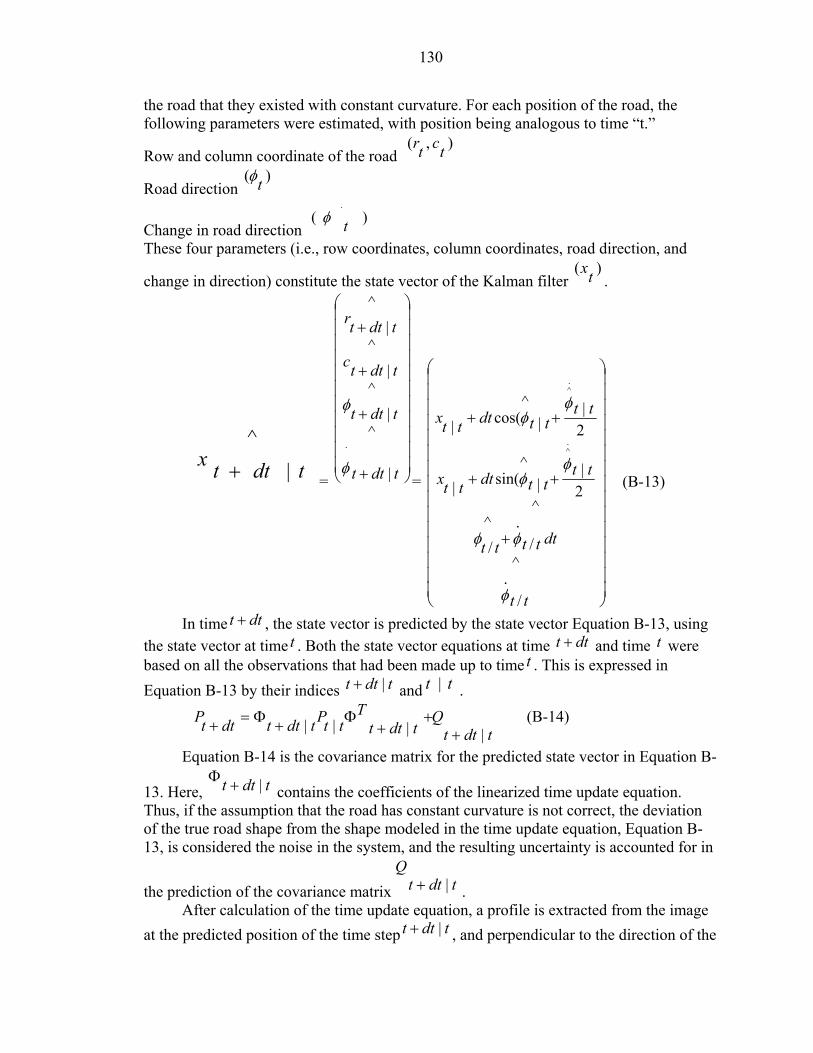
130
the road that they existed with constant curvature. For each position of the road, the following parameters were estimated, with position being analogous to time “t.”
Row and column coordinate of the road ),( tctr
Road direction )( tφ
Change in road direction )(
.
tφ
These four parameters (i.e., row coordinates, column coordinates, road direction, and
change in direction) constitute the state vector of the Kalman filter )( tx.
^| tdttx + =
+
+
+
+
^
|
^|
^|
^|
.
tdtt
tdtt
tdttc
tdttr
φ
φ
=
+
++
++
^
/.
^
/.^
/
2|
|^
sin(|
2|
|^
cos(|.^
.^
tt
dttttt
ttttdtttx
ttttdtttx
φ
φφ
φφ
φφ
(B-13)
In time dtt + , the state vector is predicted by the state vector Equation B-13, using the state vector at time t . Both the state vector equations at time dtt + and time t were based on all the observations that had been made up to time t . This is expressed in Equation B-13 by their indices tdtt |+ and tt | .
tdttQ
tdttT
ttPtdttdttP|||| +
++
Φ+Φ=+ (B-14)
Equation B-14 is the covariance matrix for the predicted state vector in Equation B-
13. Here, tdtt |+Φ contains the coefficients of the linearized time update equation.
Thus, if the assumption that the road has constant curvature is not correct, the deviation of the true road shape from the shape modeled in the time update equation, Equation B-13, is considered the noise in the system, and the resulting uncertainty is accounted for in
the prediction of the covariance matrix tdttQ
|+ . After calculation of the time update equation, a profile is extracted from the image
at the predicted position of the time step tdtt |+ , and perpendicular to the direction of the
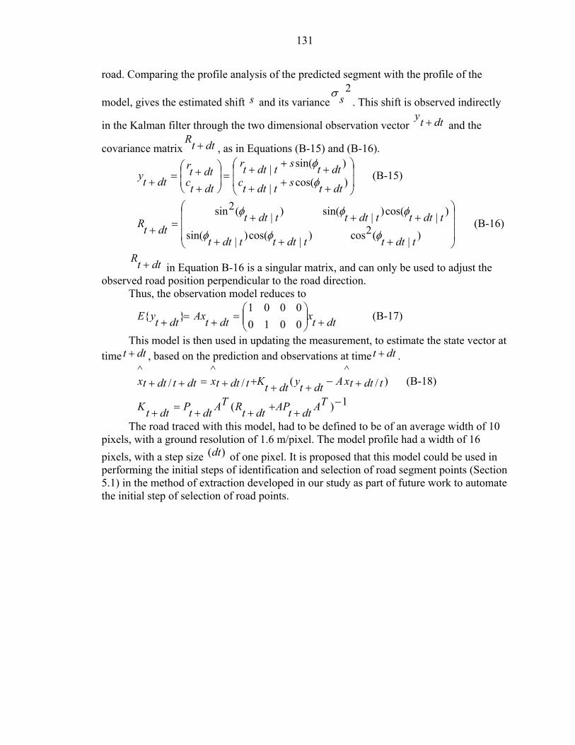
131
road. Comparing the profile analysis of the predicted segment with the profile of the
model, gives the estimated shift s and its variance2
sσ. This shift is observed indirectly
in the Kalman filter through the two dimensional observation vector dtty + and the
covariance matrix dttR + , as in Equations (B-15) and (B-16).
+++
+++=
++=+ )cos(|
)sin(|
dttstdttcdttstdttr
dttcdttr
dtty φ
φ (B-15)
+++
+++=+ )|(2cos)|cos()|sin(
)|cos()|sin()|(2sin
tdtttdtttdtt
tdtttdtttdttdttR
φφφ
φφφ (B-16)
dttR + in Equation B-16 is a singular matrix, and can only be used to adjust the observed road position perpendicular to the road direction.
Thus, the observation model reduces to
dttxdttAxdttyE +
=+=+ 0010
0001}{ (B-17)
This model is then used in updating the measurement, to estimate the state vector at time dtt + , based on the prediction and observations at time dtt + .
)/^
(/^
/^
tdttxAdttydttKtdttxdttdttx +−++++=++ (B-18)
1)( −
++++=+TAdttAPdttRTAdttPdttK
The road traced with this model, had to be defined to be of an average width of 10
pixels, with a ground resolution of 1.6 m/pixel. The model profile had a width of 16 pixels, with a step size )(dt of one pixel. It is proposed that this model could be used in performing the initial steps of identification and selection of road segment points (Section 5.1) in the method of extraction developed in our study as part of future work to automate the initial step of selection of road points.
132
LIST OF REFERENCES
Amini, A.A., T.E. Weymouth, and R.C. Jain, 1990. Using dynamic programming for solving variational problems in vision, IEEE Transactions on Pattern Analysis and Machine Intelligence, 12(9): 855-867.
Ballard, D.H., and C.M. Brown, 1982. Computer Vision, Computer Vision (P. Rose, editor), Prentice-Hall, Inc., Englewood Cliffs, N.J, pp. 1-12.
Baumgartner, A., W. Eckstein, C Heipke, S. Hinz, H. Mayer, B. Radig, C. Steger, and C. Weidemann, 1999, T-REX: TUM Research on road extraction (C. Heipke,H. Mayer, editors), Festschrift für Prof. Dr.-Ing. Heinrich Ebner zum 60. Geburtstag, Lehrstuhl für Photogrammetrie und Fernerkundung, Technische Universität München, pp 43-64.
Bebis, G., 2004. Edge contour representation, URL: http://www.cs.unr.edu/~bebis/CS791E/Notes/EdgeContourRepresentation.pdf, University of Nevada, Reno, Nevada (last date accessed: 7 August 2004).
Gruen, A., and Li, H., 1994. Semi-automatic road extraction by dynamic programming, International Archives of Photogrammetry and Remote Sensing, Vol. 30, part 3/1, pp. 324-332.
Ivins, J., and J. Porrill, 1993. Everything you wanted to know about Snakes. AIVRU technical memo #86, Artificial Intelligence Vision Research Unit, University of Sheffield, England S10 2TP.
Kass, M., A. Witkin, and D. Terzopoulos, 1988. Snakes: active contour models, International Journal of Computer Vision, 1(4): 321-331.
Malik, J., and P. Perona, 1990. Scale-space and edge detection using anisotropic diffusion, IEEE Transactions on Pattern Analysis and Machine Intelligence, 12(7):629-639.
Mayer, H., I. Laptev, and A. Baumgartner, 1998.Multi-scale and Snakes for automatic road extraction, Fifth European conference on computer vision, 2-6 June 1998, Freiburg im Breisgau, Germany.
McKeown, D.M .Jr, 1996, Top ten lessons learned in automated cartography. CMU-CS-TR, School of Computer Science, Carnegie Mellon University, Pittsburgh, PA 15213-3890.
133
McKeown Jr., D.M., and J.L. Denlinger, 1988. Cooperative methods for road tracking in aerial imagery, Defense Advanced Research Projects Agency, pp.327-341.
Rianto, Y., S. Kondo, and T. Kim, 2000, Detection of roads from satellite images using optimal search, International journal of pattern recognition and artificial intelligence, 14(8): 1009-1023.
Shukla, V., R. Chandrakanth, and R. Ramachandran, 2002. Semi-automatic road extraction algorithm for high resolution aerial images using path following approach, The III Indian Conference on Computer Vision, Graphics and Image Processing, 16-18 December 2002, Ahmedabad, India.
Simon, D., 2001. Kalman filtering, Embedded Systems Programming, 14(1): 72-79.
Trick, M.A., 1997. A Tutorial on Dynamic Programming, URL: http://mat.gsia.cmu.edu/classes/dynamic/dynamic.html, Carnegie Mellon University, Pittsburgh, PA (last date accessed: 9 August 2004).
Turton, I., 1997, Application of Pattern Recognition to Concept Discovery in Geography, M.S. Thesis, The University of Leeds, School of Geography, Leeds, United Kingdom.
Vosselman, G., and J. de Knecht, 1995.Road tracing by profile matching and Kalman filtering, Automatic extraction of Man-Made Objects from Aerial and Space Images, Birkhäuser Verlag, Basel, Switzerland, pp 265-274.
Weeratunaga, S.K., and C. Kamath, 2002. PDE-based non-linear diffusion techniques for denoising scientific and industrial images: an empirical study, Image Processing: Algorithms and Systems Conference, SPIE Electronic Imaging Symposium, 20-25 January, San Jose, California.
Weickert, J., 1999.Non-linear diffusion filtering, Handbook of Computer Vision and applications (B. Jahne, H. Haussecker and P. Geissler, editors), Academic Press, San Diego, C.A., pp. 423-450.
Wolf, P.R., and B.A. Dewitt, 2000. Elements of Photogrammetry- With Applications in GIS, McGraw-Hill, New York, 608 pp.

134
BIOGRAPHICAL SKETCH
Vijayaraghavan Sivaraman was born in Mumbai (Bombay), India, on May 2, 1979.
He obtained his bachelor’s degree in civil engineering from Regional Engineering
College, (Warangal, India) in May, 2000. He further pursued his education for a Master
of Science degree in Civil and Coastal Engineering at the University of Florida,
Gainesville. He loves watching movies, is enthusiastic about cricket, and is an ardent
follower of the Indian cricket team.