An Econometric Analysis of Donations forEnvironmental Conservation

Steven T. Yen, Peter C. Boxall and Wiktor L. Adamowicz

Staff Paper 95-04

Department of Rural EconomyFaculty of Agriculture, Forestry,And Home EconomicsUniversity of AlbertaEdmonton, Canada

RURAL ECONOMY

STAFF PAPER

An Econometric Analysis of Donations for Environmental Conservation

Steven T. YenUniversity of Illinois at Urbana-Champaign

Peter C. BoxallCanadian Forest Service

and

Wiktor L. AdamowiczUniversity of Alberta

October 1995

The purpose of the Rural Economy "Staff Papers" series is to provide a forum to accelerate thepresentation of issues, concepts, ideas, and research results within the academic and professionalcommunity. Staff Papers are published without peer review.

1

An Econometric Analysis of Donations for Environmental Conservation

I. INTRODUCTION

Funding for the protection and enhancement of the environment has traditionally come from

general tax revenues. Fish and wildlife habitat enhancement and endangered species protection are

prominent examples of this phenomenon. In the past few years, however, several aspects of this

situation have changed. First, as provincial governments have trimmed budgets, fewer funds are

available for environmental conservation programs. Second, many jurisdictions have adopted a model

by which private interests and/or users of the resource base help to fund these projects. Examples

include the North American Waterfowl Management Program, land purchases by the Nature

Conservancy, the Buck-for Wildlife project (in Alberta), and various other public-private joint

ventures (Porter and van Kooten 1993). In many of these programs the private funding component

is based on memberships or donations to private organizations (e.g. Nature Conservancy, Ducks

Unlimited). Thus, funding for conservation is relying more heavily on donations to environmental

causes either through direct giving of funds or through memberships in organizations.

For wildlife habitat management, a major environmental initiative, a third element of change

is that traditional supporters - recreational hunters and anglers - are decreasing in number, particularly

in Canada (e.g. Boxall et al. 1991). Traditionally, these supporters were responsible for much of the

funding of wildlife habitat conservation programs either through license sales, special ‘check-offs’ that

accompany license sales, or through membership fees and donations to fishing and hunting related

organizations. For example, Ducks Unlimited and Trout Unlimited began as hunting and angling

organizations respectively and much of their funding has been based on contributions from hunters

We refer to monies spent on memberships in wildlife conservation organizations as well as gifts to these organizations1

as donations, even though in the case of memberships a product is being purchased. The membership funds are typicallytargeted to support wildlife enhancement programs and thus we assume they are effectively donations to wildlife relate dcauses.

2

and anglers. With the numbers of hunters declining 17% over the last 10 years (Filion et al. 1993),

and anglers also declining over the same period (e.g. 26% in Alberta), will this traditional funding

base remain?

This paper explores some determinants of private contributions to environmental conservation

activities through an econometric analysis of donations and memberships relating to wildlife habitat

protection and enhancement. We are interested in the factors affecting donations in part because we1

wish to determine if continuing declines in the numbers of hunters and anglers will affect the level of

donations to conservation activities. We are also interested in understanding the relationships

between income, marginal tax rates (the price of donations) and other variables on the propensity to

donate. Given the increasing importance of private funding of wildlife programs, knowledge of these

relationships will be important for public and private agencies involved in wildlife conservation.

In order to examine the process generating donations for wildlife causes we employ data from

a 1991 survey conducted in the three prairie provinces that provides information on donation

behaviour, income, wildlife related activity, household compositions and a variety of other factors.

In order to fully utilize the information in this database, the analysis must consider the fact that the

vast majority of individuals do not donate to wildlife causes. Each individual is essentially facing two

decisions - a decision of whether to donate or not and a decision on how much to donate, conditional

on deciding to donate. Our econometric analysis incorporates the two-level decision structure and

the possibility of correlation between the two decision processes. We also use the model to forecast

In many U.S. states individuals are given the opportunity to give a part of their tax refund to wildlife conservatio n2

programs by writing an amount on their tax forms.

3

donations under conditions of falling hunting and angling participation rates to investigate the impact

of further declines in these activities on donations.

Previous research on wildlife donations has involved examinations of after tax check-offs in

the U.S. These studies suggest that knowledge of wildlife or in participation in wildlife related2

activity are important explanators of involvement in the check-offs (Applegate 1984; Brown et al.

1986; Manfredo and Haight 1986; Harris et al. 1992). However, these results are not directly

comparable since we are interested in donations that are considered as reductions to taxable income

(and thus individuals in different income brackets have different prices for donations). Thus, income

and other factors such as education, may play a role in the probability of donation as well as the

amount of donation. The U.S. studies, however, have not considered the joint decision to donate and

the amount of donation. They also tend to be based on small samples of individuals from specific

states. Our analysis more closely parallels the type of research performed on general donations.

Kitchen (1992) and Kitchen and Dalton (1990) examine donations in Canada. These authors

indicate that income, marginal tax rates (effectively the price of donations) and region within Canada

are factors that affect donation behaviour. Also, donation behaviour appears to be different for

religious donations than for other types of donations. Kitchen (1992) and Kitchen and Dalton (1990)

use a Tobit model framework to take into account the limited dependent variable nature of the data.

This model assumes that the decision to donate or not and the decision on the magnitude of the

donation are affected by the same parameters on the same variables. In our analysis we relax this

Maxy,c

[u(y,c;h) py qc m] ,

yt xt vt ,

4

(1)

(2)

assumption and employ a double-hurdle model to allow for the effects of independent variables to be

different in the participation and frequency portions of the donation behaviour. We also address a

concern in the literature regarding functional form in double-hurdle (or Tobit) models by employing

an inverse hyperbolic sine transformation. These models, and a more formal presentation of the

theoretical underpinnings of the situation, are described below.

II. THE MODEL

Following the literature on charitable giving, an individual's optimal donation can be derived

within the constrained utility maximization framework. That is, the individual maximizes utility

subject to a budget constraint:

where y is donation, c is a vector of other consumer goods with corresponding price vector q, h is

a vector of personal characteristics, p is the price of donation, and m is budget. Assuming the utility

function u( ) is continuous, increasing and quasi-concave, then the optimal donation can be expressed

as a function of prices and personal characteristics. Denote these determinants of donation as a

vector x and assume a linear functional form for the donation equation. Then, for individual t, the

optimal donation y can be written ast*

where is a vector of parameters and v is a random error. The demand equation (2) represents thet

‘notional’ or ‘latent’ demand for donation and is the result of utility maximization without

yt xt vt if xt vt>0

0 otherwise .

Lankford and Wyckoff (1992) accommodate skewness of the error term by using the Box-Cox transformation on the3

dependent variable.

5

(3)

nonnegativity constraints. In reality, an individual's choice is also subject to nonnegativity constraints

and therefore corner solutions could result. One way to accommodate corner solutions is to use the

Tobit model (Tobin 1958), in which case observed donation, denoted y , relates to the latent donationt

such that

The Tobit model can be estimated by the maximum likelihood (ML) method, typically by making

some distributional assumptions about the error term v (Amemiya 1985). The Tobit model has beent

used in previous studies of donation in Canada (Kitchen 1992; Kitchen and Dalton 1990), in the U.S.

(Brown 1987; Lankford and Wyckoff 1991; Reece 1979; Reece and Zieschang 1985, 1989; Schiff

1985), and in U.K. (Jones and Posnett 1991a).3

One restricted feature of the Tobit model is that a zero donation is viewed as a corner solution

in a consumer choice problem. In particular, the specification (3) suggests that the stochastic process

(and hence the sets of parameters and variables) that determines the binary outcome (participation)

also determines the level of the dependent variable. This may not apply for the case of donations.

For instance, some would never consider giving for whatever reason. In the case of specific

donations, like wildlife conservation donations, modelling the participation decision and factors

affecting participation becomes particularly important as specific individual attributes may play a large

role in explaining behaviour. But for those who choose to donate, the level of donation may well be

determined by a completely different set of factors, or in a completely different manner, from those

yt xt vt if zt ut > 0 and xt vt > 0

0 otherwise .

(ut ,vt) N(0, t ), t

1 12

122t

.

In an analysis of charitable donations by U.K. households, Jones and Posnett (1991b) used the generalized Tobit model4

(Amemiya 1985), in which zeros are determined exclusively by a binary stochastic process, that is, y = x + v if z + ut t t t t

> 0; y = 0 otherwise, where the error terms u and v are distributed as bivariate normal. Specification of the generalizedt t t

Tobit model is slightly different from that proposed by Cragg (1971), in which u and v are independent and v is zero-t t t

truncated.

6

(4)

(5)

determining the binary outcome (to give). One model that characterizes such a decision process is

the double-hurdle model--a parametric generalization of the Tobit specification. In the double-hurdle

model, the Tobit mechanism is augmented by a separate stochastic process to determine participation.

Denote the participation equation as z + u , where z is a vector of explanatory variables, is at t t

conformable parameter vector, and u is the error term. Then, the double-hurdle model can bet

expressed as:

Thus, for positive donations to occur, two hurdles have to be overcome: to participate (z + u >t t

0) and to actually donate (x + v > 0).t t4

In empirical applications of the double-hurdle model the error terms u and v in (4) are oftent t

assumed to be independently and normally distributed (Atkinson, Gomulka, and Stern 1984; Blundell

and Meghir 1987). A more generalized alternative is that the errors are distributed as bivariate

normal, viz.,

Dependence of the error terms allows interactions between the participation and level decisions and

a better characterization of the stochastic processes behind these decisions. The likelihood function

for the dependent double-hurdle model can be constructed using (4) and (5); see, for instance,

yt( ) log[ yt ( 2y 2t 1)1/2]/

sinh 1( yt)/

yt( ) xt vt if zt ut > 0 and xt vt > 0

0 otherwise .

Lyt 0

1 zt ,xt

t, t

×yt>0

1 2y 2t

1/2 1

t

yt( ) xtt

zt t

yt( ) xtt

1 2t1/2

.

7

(6)

(7)

(8)

Blundell and Meghir (1987) and Jones (1989, 1992).

In limited dependent variable models, ML estimation based on the normality assumption

produces inconsistent parameter estimates when the error terms are not normally distributed

(Robinson 1982). To allow for non-normal errors, one can consider transformations to the dependent

variable y . We use the inverse hyperbolic sine (IHS) transformation (Burbidge, Magee, and Robbt

1988)

where is an unknown parameter. Because the transformed variable is symmetric about 0 in , one

can only consider 0. The transformation is linear when approaches zero and behaves

logarithmically for large values of y for a wide range of values for . The transformation is scale-t

invariant (MacKinnon and Magee 1990), is known to be well suited for handling extreme values

(Burbidge, Magee, and Robb 1988), and avoids some of the drawbacks of the commonly used Box-

Cox transformation (MacKinnon and Magee 1990; Poirier 1978). By applying the IHS

transformation to the dependent variable y in (4), the IHS double-hurdle model can be expressed ast

Using (5), (6) and (7), the sample likelihood function for the IHS double-hurdle model is

This can be shown by using l’Hopital’s rule; see Burbidge, Magee, and Robb (1988).5

8

where ( ) and ( ) are the univariate standard normal distribution and density functions,

respectively, and ( , , ) is the bivariate standard normal distribution function. Detailed derivations

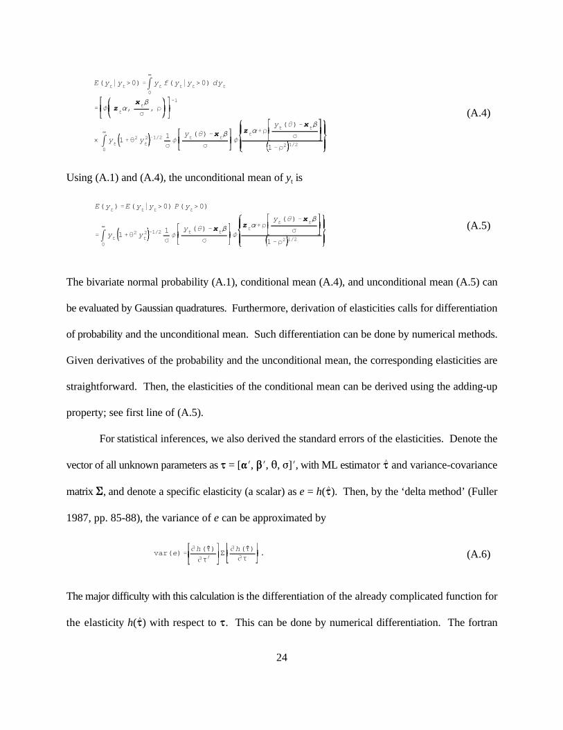
of the likelihood function, along with the expressions for the probability, conditional mean, and

unconditional mean of y , are presented in the Appendix.t

The IHS double-hurdle model includes as special cases a list of specifications used extensively

in the empirical literature. First, when = 0, y ( ) reduces to y , the jacobian term vanishes, and thet t5

model (8) reduces to the standard dependent double-hurdle model considered by Blundell and Meghir

(1987) and Jones (1989, 1992). Second, setting = 0 leads to the independent IHS double-hurdlet

model. Third, restrictions = 0 and = 0 lead to the independent double-hurdle model (Atkinson,t

Gomulka, and Stern 1984; Blundell and Meghir 1987). Fourth, setting = 0 and (z ) = 1 leadst t

to the IHS Tobit model considered by Reynolds and Shonkwiler (1991). Finally, the model obviously

reduces to the standard Tobit model (Tobin 1958) when = 0, = 0, and (z ) = 1. Because oft t

this nested structure tests of the full model against these restricted models can be done conveniently

by the likelihood-ratio tests.

III. THE DATA

Data from the 1991 National Survey on the Importance of Wildlife to Canadians (NSIWC)

for the three prairie provinces were used in this study. The 1991 survey is one of three completed

under the sponsorship of federal and provincial wildlife agencies (Filion et al. 1993), and was

conducted as a supplement to the Canadian Labour Force Survey (LFS) which is administered by

Statistics Canada on an ongoing basis (Statistics Canada 1976). The LFS is a monthly household

9

survey whose sample is representative of the civilian non-institutionalized population over 15 years

of age. The NSIWC is administered to sub-samples of the LFS sample, such that the results are

representative by province of non-institutionalized residents 15 years of age and older. Therefore,

for the three prairie provinces the 1991 survey results will accurately represent the wildlife-related

activities of 3,422,000 residents (Filion et al. 1993).

The 1991 survey involved self-administered mail back questionnaires with two follow-up

reminders and in some cases, telephone follow-ups to ensure statistically valid responses. Initial

samples sizes were 9,267 for Alberta, 7,523 for Saskatchewan and 6,955 for Manitoba and response

rates of 70.9%, 74.0%, and 70.2% were achieved respectively. Investigations of nonresponse bias

suggested nonrespondents were not restricted to specific groups of individuals, nor were they located

in specific geographic areas (Yiptong and DuWors 1990). Completed questionnaires were processed

under rigorous protocols which included exhaustive edit procedures to identify erroneous records and

ensure data quality, and a method to match respondent demographic data from the LFS to their

NSIWC survey answers. Measures of statistical confidence were conducted such that all information

used satisfies a minimum level of reliability. Further details on the survey can be found in Filion et

al. (1993) and Yiptong and DuWors (1990).

Information from 13,572 individuals was extracted from this database and a set of variables

thought to influence their wildlife donations was devised (Table 1) based upon previous studies (e.g.

Applegate 1984; Brown et al. 1986; Manfredo and Haight 1986; Harris et al. 1992). Note that these

independent variables are generally of three types: socioeconomic (income, education, etc.),

attitudinal (attitude indices on wildlife preservation, etc.), and participatory (days and expenditures

spent on wildlife activities). In order to compare our findings with previous studies of donation

Analytic derivatives of the log-likelihood function are available from the authors.6

10

behaviour (e.g. Kitchen 1992) and to develop elasticities across various socioeconomic groups, we

stratified the sample into three income groups: low, which includes those reporting personal 1991

income ranging from $0 to $9,999; medium, where it ranged from $10,000 to $29,999, and high

where it ranged from $30,000 to over $50,000. In addition, the ‘price’ of a donation was calculated

as 1 marginal tax rate. For each individual in the sample their marginal tax rate was calculated based

on standard deductions for the 1991 tax year.

Sample statistics of variables in the income strata and for the entire sample are shown in Table

2. For the full sample 10.1% of the individuals reported a donation and the average amount per

individual was $0.78. However, the average amount for those reporting a positive donation was

$7.77. The participation in donating, and the amount donated, increases across the income strata.

IV. RESULTS OF ESTIMATION

Parameter Estimates

We estimate the dependent IHS double-hurdle model for all three income strata and for the

full sample. ML estimation was carried out by maximizing the logarithm of the likelihood function

(8), using the quadratic hill-climbing algorithm (Goldfeld, Quandt and Trotter 1966). The full sets6

of parameter estimates are presented in Table 3.

The IHS parameter ( ) is significantly different from 0 for all samples considered, suggesting

that the standard (untransformed) double-hurdle specification would be misspecified. For the low-

income stratum, the covariance parameter ( ) is significant at the 0.10 level of significance; thus the12

consideration for dependence between the participation and level decisions is justified. The

11

covariance is not significant for the other income strata or the full sample, however.

For the low income stratum the propensity to donate is significantly affected by 3 variables

which reflect direct or incidental involvement with wildlife-related activities. In contrast, the level

of donations for the stratum are affected by education level, gender, residence in a rural area, and

expenditures - only one of the involvement variables (Days residence) affects both the participation

and level of donation. The paucity of explanatory variables in either of the hurdles for the low income

group probably mirrors their low involvement in donation activity (Table 2).

For the medium- and high-income strata, however, more variables become significant in both

of the donation decisions. For participation, the socioeconomic variables Education, Age, Rural, and

Male affect participation in the medium stratum, while only Rural does for high income earners. Of

the attitudinal variables only Preserving influences participation in the high income stratum, but only

at the 10% level of significance. Almost all of the intensity-of-participation variables affect donation

participation in both strata. In explaining the level of donation, age and residence in a rural area affect

medium income individuals, while income level and education do so for those in the high income

group. Attitudes towards wildlife abundance affect the donation level in both strata, as do days spent

on nonconsumptive activity in the province, days in incidental wildlife encounters, and total

expenditures on wildlife-related activities.

Significant parameters across the income groups include (1) days spent fishing affect the

participation decision in each stratum; (2) days spent incidentally encountering wildlife and days spent

on wildlife activities around residences or cottages affect one or both of the donation decisions in

each income group; and (3) total expenditure levels on wildlife-related activities affect the level of

donation, but not participation in donating in each stratum.

Our procedure is similar to that of McDonald and Moffitt (1980), who examine the effects explanatory variables for the7

standard Tobit model.

12

It is noteworthy that the parameter estimates on tax price were not significantly different from

0 for either donation decision in each stratum. This finding also appears for the tax price parameter

in the full sample model (Table 3). The full sample model also suggests that income is important in

the level of donation and an apparent negative influence is associated with residing either in Alberta

or Manitoba (relative to Saskatchewan).

Examining the Effects of Variables

In limited dependent variable models, it is typically difficult to quantify the effects of

explanatory variables on the dependent variable. This is particularly true for the models considered

in this study because the double-hurdle parameterization, the dependent error specification, and the

IHS transformation all complicate the effects of explanatory variables. In fact, detailed quantitative

effects of explanatory variables have often been overlooked in previous applications of double-hurdle

models. In this study, we examine the probability of participation in donation and the mean donation

conditional and unconditional on participation, and derive the elasticities of these components with

respect to all continuous explanatory variables. All elasticities are calculated at the sample means7

of variables. For statistical inferences, the standard errors for these elasticities are also derived using

mathematical approximation (Fuller 1987). The expressions for the probability and the means,

conditional and unconditional on participation, along with the derivation of elasticities and the

standard errors for these elasticities, are presented in the Appendix. For binary explanatory variables

the elasticities are not strictly defined. The values reported in the table of elasticities are actually

13

changes in the dependent variable in response to the change in the binary variable from zero to one.

For each binary variable we assess the impact of a finite change (i.e., from zero to one) on the

probability of donation, the amount of donation conditional on choosing to donate, and on the

unconditional donation amount, while holding all other variables constant at their sample means.

The elasticities with respect to continuous variables are presented in Table 4. Income has

significant and positive effects only on the probability (but not the conditional level) of donation for

individuals in the medium-income stratum, but the elasticity is high. In particular, a one percent

increase in income increases the probability of donation by about 2.01 percent. Consequently, the

elasticity of the unconditional level is also quite high, with a one percent increase in income leading

to a 2.45 percent increase in donation. For the high-income stratum, the effect of income on both

probability and conditional level (and therefore the unconditional level) of donation are positive and

significant, although the elasticities are much lower than those of the medium-income individuals.

For the high-income individuals, a one percent increase in income increases the probability of

donation by only about 1.07 percent, the conditional level of donation by 0.67 percent, and the

unconditional level of donation by 1.73 percent. The statistical insignificance of elasticities suggests

income does not play a role on the donation behavior among the low-income individuals.

For the full sample, the income elasticities of all three components (probability and levels) of

donation are significant and positive but are much smaller than the corresponding elasticities in the

medium- and high-income samples. These relatively low elasticities are obviously the results of low

responses to income among the low-income individuals.

Total expenditures have significant and positive effects on probability and levels of donation,

although the elasticities are very small, ranging from 0.01 to 0.06. Education and age have positive

14

effects on donation, with the medium-income individuals being more responsive to changes in these

two variables than other individuals.

Among the attitudinal variables, Abundance has positive effects on probability and levels of

donation for both medium- and high-income individuals. Preserving has positive effects on donation

only among the medium-income individuals.

Regarding participation in wildlife-related activity, significant positive effects occur for

involvement in residential wildlife activity for two strata, nonconsumptive participation for the high

income group, and hunting activity for the top two income strata. Tax price remains statistically

insignificant across all income strata.

The effects of binary variables on donation are presented in Table 5. Residence in rural areas

have negative effects on donations for the high income strata, and also for the full sample. An

interesting finding is that residence in Alberta and Manitoba negatively affects donation probability

in all four models. A corollary of this result of course, is that residents in Saskatchewan are more

likely to donate than residents in the other two Provinces.

Simulating Changes in Wildlife Donations

We used the estimated model to simulate the impacts of declines in three variables that affect

donation behavior. We chose Income and Total Expenditures because of their statistical significance

across the income strata in explaining donation behavior, and Days Hunting given its performance

in the model and because participation in hunting has been thought by many wildlife managers to

influence donations. The scenario examined for each variable was a reduction in its mean value by

A 15% change in income could be considered severe. However, we are attempting to compare changes of simila r8

magnitude in important explanators of donation behaviour.

15

15%. The effect of a reduction was investigated by calculating donations (both conditional and8

unconditional on donating) before and after the reduction using the estimated parameters and the

mean values of the all other variables in each stratum. In order to portray the findings in a meaningful

context, the results are reported for each stratum by aggregating the unconditional probability results

over the total population of the three provinces (Table 6).

Declines of 15% in income have large effects on donations. For the medium and high income

groups (about 62% of the sample) this income reduction reduces the probability of donating by 3.84%

and 5.12% in the medium and high income groups respectively. Conditional on the decision to

donate, this reduces the estimated amount donated from $45.55 to $42.55 (a drop of $3.00) per

individual in the medium income stratum, and from $71.71 to $65.07 (a drop of $6.64) per individual

in the high income stratum. Unconditional on the decision to donate, the income reduction results

in individual donations declining from $5.69 to $3.83, and $23.83 to $18.29 for the income groups

respectively. In aggregate terms, wildlife managers and organizations could expect reductions in

donations of $2.35 million by middle income earners and $4.74 million by high income earners given

a 15% decline in income in the three provinces (Table 6). Using the full sample model, this aggregate

impact is estimated to be about $4.7 million.

Reductions in Days Hunting and Total Expenditures have much less impact on donations than

reductions in income (Table 6). Hunting participation declines have more impact than expenditures

in the middle income stratum, while expenditures have a greater effect than hunting participation in

the high income stratum. These results, of course, are due to the differences in the parameter

16

estimates in the two models (Table 4).

V. DISCUSSION

Zero observations are common features of microdata. The Tobit model has the undesirable

parametric restrictions that limit its use in empirical investigations. Most previous studies of donation

behavior were based on the Tobit model. Yet donation is one area where the decisions to donate and

how much to donate are most likely to be made differently. The IHS double-hurdle model we

consider in this study accommodates such decision structure; it also allows for nonnormality in the

error distribution.

The double-hurdle model has been used frequently in microeconometric modelling. However,

the empirical results in these studies have not been fully explored because the parameter estimates

alone do not reveal a complete picture of the effects of explanatory variables on the dependent

variable. We explore the effects of explanatory variables by examining the probability of donating,

and the conditional and unconditional level of donations and deriving the elasticities of these

components with respect to the explanatory variables. Such decomposition of elasticities is

particularly important when the participation and level decisions are correlated and when the

dependent variable is transformed, as is the case in the present study.

We believe our findings have some important implications for donations to wildlife

conservation. First, in two income strata and the full sample income has the largest effect on donation

probability and the conditional and unconditional levels (Table 4). This suggests that recessions may

have the most important negative impacts on wildlife donations. This is supported by the fact that

total expenditures on wildlife-related activities, which are also affected by economic declines, also

17

play an important, although smaller, role in donations. Our results suggest that the effect of income

declines may not be offset by increases in participation in various wildlife-related activities.

A related finding here is the observation that tax prices were not significant in explaining

donations to wildlife conservation. Kitchen (1992) and Kitchen and Dalton (1990) found similar

results in explaining Canadian donations to religious causes. This raises an intriguing question about

the degree of similarity of religious and wildlife conservation motives in terms of financial support.

On the other hand, this similarity may be related to the fact that these types of donations are focused

on specific issues or targets, and are not donations to some more broad-based causes (e.g. poverty).

Second, declines in hunting and angling activity were not found to be as significant in affecting

donations as we suspected a priori. While angling days were found to be statistically insignificant

in explaining donation behavior, hunting days were significant for only the higher income strata.

Declines in hunting do suggest an impact on donations, but this impact may not be as large as many

wildlife managers suspect.

On the other hand, changes in participation in other types of wildlife activity may have

significant effects on donations. For example, involvement in residential wildlife activities,

particularly by people in lower and medium-income strata, was found to affect donation behaviour.

This activity has been generally overlooked by wildlife management agencies (Boxall and McFarlane

1995; Shaw et al. 1985) and encouraging greater levels of participation in these activities may serve

to increase donations. Similarly, participation in nonconsumptive activities, such as taking trips to

view wildlife both inside and outside the province of residence, may affect positively donation

behaviour. Our findings suggest this may be the case for those earning high incomes. These results

have important implications for recent efforts by governments and the private sector to increase levels

18

of ecotourism and ecotourism business opportunities. Increased ecotourism levels may not only

promote economic development, but may also serve to increase financial support for wildlife

management efforts through donations. Whether changes in nonconsumptive activities can offset

declines in donations due to reductions in hunting and fishing activity is an open question, however.

Third, a set of factors that do seem to influence donations are attitudes towards wildlife

abundance and preservation, as well as interest in being involved in wildlife-related activity. These

findings generally mirror those of U.S. researchers who examine tax check-offs (e.g. Applegate 1984;

Brown et al. 1986; Manfredo and Haight 1986; Harris et al. 1992). The importance of attitudinal

variables, in conjunction with the apparent significance of education (Tables 2 and 3), suggests that

in a climate of declining budgets and government involvement in wildlife management, education

efforts directed towards wildlife attitudes and interests may significantly affect private donations.

Finally, we derived an intriguing result which suggests that residents of Saskatchewan are

more likely to donate than Albertans or Manitobans. This may be related to a combination of

conditions such as: i) unique cultural factors inherent in the history of that province; ii) the fact that

more of Saskatchewan's population is rural rather than urban; and iii) the fact that Saskatchewan's

major private wildlife organization involves both consumptive and nonconsumptive wildlife

recreationists, in contrast to the similar organizations in Alberta and Manitoba.

VI. CONCLUSIONS

In this paper we examine wildlife donations in a manner consistent with economic theory, and

utilize econometric methods which effectively capture the varying effects of the probability of

participation and the amount. The economic literature on general donations has not utilized

19

econometric methods that capture these effects. Previous studies in the wildlife management

literature have used very simple models, and have not generally examined the economic issues of

donations. Thus our study makes a contribution to both the applied economics and resource

management literatures.

Our empirical results suggest that changes in economic activity will be much more important

than changes in participation in any wildlife-related activity. However, declines in hunting and angling

will have impacts on donations to conservation causes, but these impacts are not large. Given

observed declines in participation in consumptive uses, and increased participation in nonconsumptive

uses, reductions in donations from one may be offset by increases from the other. The information

required to analyze this issue in detail, however, was beyond the scope of our study. While there are

calls for the traditional focus of wildlife management agencies on consumptive users to broaden to

include other types of wildlife users, this debate has generally focused on the issue of the revenue

captured by the agency. Wildlife managers should realize that their efforts to provide service to and

influence other types of wildlife users may also influence the revenue available to private wildlife

conservation organizations.

REFERENCES

Amemiya, T. (1985) Advanced Econometrics (Cambridge: Harvard University Press)

Applegate, J.E. (1984) ‘Nongame tax check-off programs: a survey of the New Jersey residentsfollowing the first year of contributions.’ Wildlife Society Bulletin 12, 122-28

Atkinson, A.B., J. Gomulka, and N.H. Stern (1984) ‘Household expenditure on tobacco 1970-1980:evidence from the Family Expenditure Survey.’ ESRC Programme on Taxation, Incentives,and the Distribution of Income, London School of Economics, Discussion Paper No. 60.

20

Blundell, R.W., and C. Meghir (1987) ‘Bivariate alternatives to the univariate Tobit model.’ Journalof Econometrics 33, 179-200

Boxall, P.C., E. Duwors, and F.L. Filion (1991) ‘Trends and factors influencing participation inrecreational hunting in Canada: a dynamic model.’ In Transactions of the XXth Congress ofthe International Union of Game Biologists, pp. 658-669, eds., S. Csanyi and J. Ernhaft.University of Agricultural Sciences, Godollo, Hungary.

Boxall, P.C., and B.L. McFarlane (1995) ‘Analysis of discrete dependent variables in humandimensions research: participation in residential nonconsumptive activity.’ Wildlife SocietyBulletin 23, 283-89

Brown, E. (1987) ‘Tax incentives and charitable giving: evidence from the new survey data.’ PublicFinance Quarterly 15, 386-96

Brown, T.L., N.A. Connelly, and D.J. Decker (1986) ‘First-year results of New York's return a giftto wildlife tax checkoff.’ Wildlife Society Bulletin 14, 115-20

Burbidge, J.B., L. Magee, and A.L. Robb (1988) ‘Alternative transformations to handle extremevalues of the dependent variable.’ Journal of the American Statistical Association 83, 123-27

Cragg, J.G. (1971) ‘Some statistical models for limited dependent variables with applications to thedemand for durable goods.’ Econometrica 39, 829-44

Filion, F.L., E. DuWors, P. Boxall, P. Bouchard, R. Reid, P.A. Gray, A. Jacquemot, and G. Legare(1993) ‘The importance of wildlife to Canadians: highlights of the 1991 survey.’ CanadianWildlife Service, Environment Canada, Ottawa.

Fuller, W.A. (1987) Measurement Error Models (New York: John Wiley & Sons)

Goldfeld, S.M., R.E. Quandt, and H.F. Trotter (1966) ‘Maximization by quadratic hill-climbing.’Econometrica 34, 541-51

Harris, C.C., T.A. Miller and K. Reese (1992) ‘Possible influences on donation behavior: the caseof Idaho’s nongame wildlife and endangered species tax checkoff fund.’ Society and NaturalResources 5, 53-66

Jones, A.M., and J.W. Posnett (1991a) ‘The impact of tax deductibility on charitable giving bycovenant in the UK.’ Economic Journal 101, 1117-29

Jones, A.M., and J.W. Posnett (1991b) ‘Charitable donations by UK households: evidence from theFamily Expenditure Survey.’ Applied Economics 23, 343-51

21

Jones, A.M. (1989) ‘A double-hurdle model of cigarette consumption.’ Journal of AppliedEconometrics 4, 23-39

Jones, A.M. (1992) ‘A note on computation of the double-hurdle model with dependence with anapplication to tobacco expenditure.’ Bulletin of Economic Research 44, 67-74

Kitchen, H. (1992) ‘Determinants of charitable donations in Canada: a comparison over time.’Applied Economics 24, 709-13

Kitchen, H., and R. Dalton (1990) ‘Determinants of charitable donations by families in Canada: aregional analysis.’ Applied Economics 22, 285-99.

Lankford, R.H., and J.H. Wyckoff (1991) ‘Modeling charitable giving using a Box-Cox standardTobit model.’ Review of Economics and Statistics 73, 460-70

MacKinnon, J.G., and L. Magee (1990) ‘Transforming the dependent variable in regression models.’International Economic Review 31, 315-39

Manfredo, M.J., and B. Haight (1986) ‘Oregon’s nongame tax checkoff: a comparison of donorsand nondonors.’ Wildlife Society Bulletin 14, 121-26

Poirier, D.J. (1978) ‘The use of the Box-Cox transformation in limited dependent variable models.’Journal of the American Statistical Association 73, 284-87

Porter, R.M., and G.C. van Kooten (1993) ‘Wetlands preservation on the Canadian prairies: theproblem of the public duck.’ Canadian Journal of Agricultural Economics 41, 401-10

Reece, W.S. (1979) ‘Charitable contributions: new evidence on household behavior.’ AmericanEconomic Review 69, 142-51

Reece, W.S., and K.D. Zieschang (1985) ‘Consistent estimation of the impact of tax deductibilityon the level of charitable contributions.’ Econometrica 53, 271-93.

Reece, W.S., and K.D. Zieschang (1989) ‘Evidence on taxation and charitable giving from the 1983U.S. Treasury tax model file.’ Economics Letters 31, 49-53

Reynolds, A., and J.S. Shonkwiler (1991) ‘Testing and correcting for distributional misspecificationsin the Tobit model: an application of the information matrix test.’ Empirical Economics 16,313-23

Robinson, P.M. (1982) ‘On the asymptotic properties of estimators of models containing limiteddependent variables.’ Econometrica 50, 27-41

22

Schiff, J. (1985) ‘Does government spending crowd out charitable contributions?’ National TaxJournal 38, 535-46

Shaw, W.W., W.R. Mangun, and J.R. Lyons (1985) ‘Residential enjoyment of wildlife resources byAmericans.’ Leisure Sciences 7, 361-75

Statistics Canada (1976) ‘Methodology of the Canadian Labour Force Survey.’ Catalogue #71-326,Statistics Canada, Ottawa.

Tobin, J. (1958) ‘Estimation of relationships for limited dependent variables.’ Econometrica 26,24-36

Yiptong, J., and E. DuWors (1990) The Importance of Wildlife to Canadians in 1987: A User'sGuide to the Methodology of a National Survey. Canadian Wildlife Service, EnvironmentCanada, Ottawa.

P(yt>0) P(ut> zt ,vt> xt ) zt ,xt , ,

f(yt ut> zt ,vt> xt )zt

f(ut,yt ut> zt ,vt> xt )dut

zt

f(ut,yt) zt ,xt ,

1

dut zt ,xt ,

1

1 2y 2t

1/2

zt ,xt ,

1

1 2y 2t

1/2 1 yt( ) xtzt

yt( ) x

1 2 1/2

Lyt 0

[1 P(ut> zt ,vt> xt )]

×yt>0

f(yt ut> zt ,vt> xt ) P(ut> zt ,vt> xt ) .

23

(A.1)

(A.2)

(A.3)

APPENDIX

Likelihood Function, Probability and Means of y , and Calculation of Elasticitiest

Based on the IHS double-hurdle structure (7) and the bivariate normality assumption of errors

(5), the probability of a positive observation is

where = / . The conditional density of y can be derived as follows:t 12 t

In (A.2), the term (1 + y ) is the Jacobian of transformation from (u , y ) to (u , v ). The2 2 -1/2t t t t t

integration can be accomplished by writing f(u ,v ) = f(v ) f(u |v ) and then integrating out thet t t t t

unobserved u . The sample likelihood function for an independent sample ist

Substituting (A.1) and (A.2) into (A.3) gives the sample likelihood function (8).

The interpretation of results calls for the expressions for the probability, conditional mean,

and unconditional mean of y . Using the conditional distribution (A.2), the conditional mean of y ist t

E(yt yt>0)0

yt f(yt yt>0) dyt

zt ,xt ,

1

×0

yt 12 y 2

t1/2 1 yt( ) xt

zt

yt( ) xt

1 2 1/2

E(yt) E(yt yt>0) P(yt>0)

0

yt 12 y 2

t1/2 1 yt( ) xt

zt

yt( ) xt

1 2 1/2

var(e) h(ˆ) h(ˆ) .

24

(A.4)

(A.5)

(A.6)

Using (A.1) and (A.4), the unconditional mean of y ist

The bivariate normal probability (A.1), conditional mean (A.4), and unconditional mean (A.5) can

be evaluated by Gaussian quadratures. Furthermore, derivation of elasticities calls for differentiation

of probability and the unconditional mean. Such differentiation can be done by numerical methods.

Given derivatives of the probability and the unconditional mean, the corresponding elasticities are

straightforward. Then, the elasticities of the conditional mean can be derived using the adding-up

property; see first line of (A.5).

For statistical inferences, we also derived the standard errors of the elasticities. Denote the

vector of all unknown parameters as = [ , , , ] , with ML estimator and variance-covariance^

matrix , and denote a specific elasticity (a scalar) as e = h( ). Then, by the ‘delta method’ (Fuller^

1987, pp. 85-88), the variance of e can be approximated by

The major difficulty with this calculation is the differentiation of the already complicated function for

the elasticity h( ) with respect to . This can be done by numerical differentiation. The fortran^

25

program for computation of the elasticities and the standard errors for elasticities is available from

the authors.

26

Table 1. Definitions of variables used to examine donations to wildlife conservation in three provinces inCanada from the 1991 National Survey on the Importance of Wildlife to Canadians.

Variable Definition

Donation Amount spent, in tens of dollars, on membership fee(s) or donation(s) during 1991; dependentvariable

Income Personal income before deduction (1 = 0; 8 = $50,000 or more)

Education Level of education (1 = 0-8 years; 6 = university degree)

Age group Age group (1 = 15-16 years; 13 = 70 years or over)

Rural Resides in a rural community with less than 10,000 people (dummy variable where 1 = yes; 0 =no)

Male Individual is male (dummy variable where 1 = yes; 0 = no)

Head Individual is a head of household (dummy variable where 1 = yes; 0 = no)

Abundance Index of importance of abundance of wildlife a

Preserving Importance of preserving declining or endangered wildlife (0 = not important; 3 = veryimportant)

Some interest At least some interest in wildlife activities (dummy variable where 1 = yes; 0 = no)b

Days residence Number of days spent on wildlife activities around residence or cottage in 1991 (1=1 to 9 days;7=200 days or more)

Days in province Number of days spent on trips inside province of residence in 1991 where the primary purposeof the trip was to encounter wildlife (watching, feeding, photographing or studying wildlife)

Days outside prov Number of days spent on trips outside province of residence in 1991 where the primary purposeof the trip was to encounter wildlife (watching, feeding, photographing or studying wildlife)

Days incidental Number of days spent on trips in Canada in 1991 where wildlife was observed, but the mainpurpose of the outings was other than encountering wildlife (e.g., hiking/picnics) (1=1-9 days;7=200+ days)

Days hunting Number of days spent hunting in Canada during 1991

Days fishing Number of days spent fishing in freshwater, lakes, rivers, or streams in Canada during 1991

Total expenditures Total expenditures on fish and wildlife activities in $100 (imputed)

Tax price Tax price (calculated as 1 estimated marginal tax rate)

Alberta Resides in Alberta (dummy variable where 1 = yes; 0 = no)

Manitoba Resides in Manitoba (dummy variable where 1 = yes; 0 = no)

Derived as the sum of scores indicating importance for abundance of waterfowl, other birds, small mammals, and largea

mammals, each with a value ranging from 0 (not important) to 3 (very important). Activities include watching, photographing, studying, feeding, hunting, and trapping wildlife; collecting specimens; andb

observing, collecting, creating wildlife-related art/literature.

27

Table 2. Sample Statistics

Low-income Medium-income High-income Full sample

Variable Mean St. dev. Mean St. dev. Mean St. dev. Mean St. dev.

Donation 0.261 1.800 0.724 6.176 1.642 15.721 0.784 8.852(4.782) (6.155) (6.994) (18.040) (9.940) (37.623) (7.770) (26.888)a a a a a a a a

Income 2.109 0.772 4.451 0.498 6.922 0.857 4.204 2.008Education 2.883 1.422 3.478 1.517 4.205 1.537 3.440 1.574Age group 6.048 3.892 7.083 3.202 7.079 2.351 6.696 3.336Rural 0.515 0.448 0.414 0.465b

Male 0.302 0.482 0.755 0.484b

Head 0.264 0.571 0.784 0.511b

Abundance 8.761 3.875 9.351 3.512 9.956 2.962 9.284 3.556Preserving 2.220 1.002 2.352 0.899 2.471 0.759 2.333 0.912Some interest 0.769 0.805 0.872 0.809b

Days residence 2.036 2.237 2.255 2.276 2.375 2.228 2.204 2.254Days in Province 2.680 17.408 3.536 19.458 3.846 18.698 3.295 18.528Days outside Prov. 0.372 4.858 0.444 3.489 0.679 4.375 0.477 4.267Days incidental 0.625 1.037 0.754 1.120 0.933 1.231 0.751 1.126Days hunting 1.040 9.463 1.358 6.939 2.191 10.135 1.450 8.809Days fishing 2.417 9.797 3.766 11.377 4.969 14.610 3.568 11.800Total expenditures 1.912 10.594 4.472 27.297 8.521 41.362 4.543 27.574Tax price 0.924 0.105 0.712 0.015 0.576 0.020 0.757 0.154Alberta 0.373 0.394 0.446 0.399b

Manitoba 0.303 0.286 0.243 0.281b

Sample size 5059 5075 3438 13572Number donating 276 (5.5%) 525 (10.3%) 568 (16.5%) 1369

Computed from the sub-samples of donating individuals.a

Dummy variablesb

28

Table 3. ML Estimation of IHS Double Hurdle Modela

Low-income Medium-income High-income Full sample

Variable Particip. Level Particip. Level Particip. Level Particip. Level

Constant 1.805 19.741** 4.947 19.186 3.874 20.333 1.782 23.542**(2.392) (8.529) (5.740) (21.418) (9.703) (39.412) (1.144) (4.188)

Income 0.197 0.924 0.365 0.805 0.071 0.995* 0.036 0.823**(0.268) (0.829) (0.235) (0.940) (0.135) (0.536) (0.061) (0.229)

Education 0.083 0.414* 0.192** 0.220 0.003 0.565** 0.087** 0.431**(0.066) (0.246) (0.063) (0.211) (0.055) (0.215) (0.035) (0.129)

Age 0.032 0.158 0.056* 0.210* 0.053 0.229 0.043** 0.206**(0.028) (0.109) (0.033) (0.119) (0.038) (0.151) (0.020) (0.076)

Rural 0.125 1.438** 0.683** 1.199* 0.373** 0.777 0.363** 0.310(0.212) (0.714) (0.189) (0.682) (0.167) (0.656) (0.105) (0.399)

Male 0.422 1.853** 0.439** 1.349 0.048 0.817 0.254* 0.604(0.268) (0.827) (0.224) (0.869) (0.221) (1.069) (0.136) (0.538)

Head 0.293 0.246 0.027 0.614 0.234 0.750 0.029 0.042(0.257) (0.822) (0.203) (0.763) (0.206) (0.977) (0.134) (0.514)

Abundance 0.018 0.256 0.028 0.428** 0.003 0.374** 0.006 0.357**(0.044) (0.185) (0.051) (0.183) (0.041) (0.177) (0.026) (0.098)

Preserving 0.008 0.408 0.127 1.179* 0.282* 0.987 0.143 0.529(0.171) (0.628) (0.197) (0.691) (0.154) (0.667) (0.100) (0.390)

Some interest 0.365 2.116 0.141 1.727 0.446 1.578 0.539 4.546**(0.608) (2.683) (0.552) (2.308) (0.475) (3.443) (0.524) (1.760)

Days residence 0.074* 0.264* 0.029 0.399** 0.143** 0.130 0.091** 0.247**(0.041) (0.158) (0.042) (0.154) (0.042) (0.148) (0.025) (0.090)

Days in Province 0.004 0.014 0.006** 0.024** 0.007* 0.039** 0.004** 0.022**(0.006) (0.013) (0.003) (0.010) (0.003) (0.012) (0.002) (0.006)

Days outside Prov. 0.403 0.019 0.145** 0.035 0.202** 0.075* 0.242** 0.037(0.303) (0.054) (0.052) (0.036) (0.093) (0.042) (0.083) (0.024)

29

Days incidental 0.244** 0.077 0.408** 0.476** 0.255** 0.653** 0.271** 0.291**(0.110) (0.241) (0.090) (0.211) (0.112) (0.244) (0.068) (0.144)

Days hunting 1.186 0.007 0.451** 0.028 3.053 0.045** 1.949 0.028**(1.229) (0.016) (0.165) (0.020) (2.222) (0.016) (1.322) (0.009)

Days fishing 0.064** 0.016 0.027** 0.002 0.028** 0.002 0.038** 0.003(0.027) (0.011) (0.009) (0.014) (0.012) (0.012) (0.008) (0.007)

Total expenditures 0.001 0.042** 0.004 0.026** 0.001 0.028** 0.001 0.024**(0.006) (0.011) (0.002) (0.008) (0.001) (0.005) (0.001) (0.003)

Tax price 0.072 2.143 11.015 1.875 10.693 1.221 0.325 4.439(1.698) (5.846) (9.085) (34.240) (15.860) (64.359) (0.854) (3.173)

Alberta 0.338 0.288 0.196 2.316** 0.258 0.557 0.009 1.462**(0.244) (0.840) (0.215) (0.081) (0.572) (2.329) (0.125) (0.466)

Manitoba 0.330 0.152 0.261 2.018** 0.134 0.841 0.057 1.091**(0.241) (0.794) (0.251) (0.873) (0.264) (1.066) (0.131) (0.475)

5.610** 6.273** 7.068** 6.550**(0.760) (0.518) (0.564) (0.345)

12 2.263* 1.606 1.082 0.651(1.269) (1.157) (1.154) (0.767)0.200** 0.205** 0.179** 0.195**

(0.044) (0.021) (0.020) (0.014)Log likelihood 1586.680 2805.620 2992.432 7437.493

Asymptotic standard errors in parentheses.a

** Significant at 5% level.* Significant at 10% level.

30

Table 4. Elasticities With Respect to Continuous Variables a

Low-income Medium-income High-income Full sample

Variable Prob. level level Prob. level level Prob. level level Prob. level levelCond. Uncond. Cond. Uncond. Cond. Uncond. Cond. Uncond.

Income 0.442 0.212 0.654 2.011** 0.465 2.477** 1.065* 0.665* 1.730* 0.767** 0.308** 1.074**

(0.516) (0.214) (0.623) (0.666) (0.333) (0.917) (0.576) (0.354) (0.924) (0.214) (0.084) (0.297)

Education 0.424** 0.088 0.512** 0.660** 0.125* 0.785** 0.367** 0.229** 0.597** 0.333** 0.133** 0.466**

(0.192) (0.081) (0.249) (0.147) (0.066) (0.177) (0.137) (0.088) (0.222) (0.097) (0.039) (0.135)

Age 0.339* 0.070 0.409* 0.636** 0.171** 0.807** 0.251 0.157 0.408 0.310** 0.123** 0.434**

(0.181) (0.072) (0.235) (0.129) (0.069) (0.175) (0.166) (0.104) (0.269) (0.110) (0.045) (0.154)

Abundance 0.706* 0.190 0.896 0.761** 0.355** 1.116** 0.576** 0.360** 0.935** 0.731** 0.294** 1.025**

(0.393) (0.164) (0.549) (0.219) (0.129) (0.318) (0.281) (0.166) (0.444) (0.202) (0.078) (0.278)

Preserving 0.270 0.081 0.351 0.443** 0.237* 0.679** 0.377 0.235 0.612 0.279 0.111 0.390

(0.333) (0.153) (0.477) (0.205) (0.123) (0.294) (0.259) (0.158) (0.415) (0.196) (0.079) (0.275)

Days residence 0.204** 0.036 0.240** 0.261** 0.090** 0.350** 0.048 0.030 0.078 0.124** 0.049** 0.173**

(0.104) (0.040) (0.122) (0.050) (0.026) (0.070) (0.055) (0.034) (0.089) (0.048) (0.018) (0.065)

Days in Province 0.008 0.004 0.012 0.006 0.006** 0.012 0.023** 0.014** 0.038** 0.016** 0.006** 0.022**

(0.012) (0.005) (0.013) (0.008) (0.003) (0.010) (0.007) (0.004) (0.011) (0.004) (0.002) (0.006)

Days outside Prov. 0.044 0.014 0.031 0.043** 0.004 0.046** 0.008* 0.005* 0.013* 0.002 0.001 0.003

(0.088) (0.028) (0.063) (0.018) (0.004) (0.019) (0.004) (0.003) (0.007) (0.011) (0.002) (0.013)

Days incidental 0.062 0.009 0.053 0.135** 0.009 0.126** 0.094** 0.059** 0.153** 0.044 0.019* 0.063

(0.089) (0.033) (0.075) (0.057) (0.018) (0.059) (0.034) (0.022) (0.055) (0.030) (0.010) (0.039)

Days hunting 0.381 0.107 0.274 0.447** 0.052 0.500** 0.015** 0.010** 0.025** 0.065 0.014 0.079

(0.340) (0.135) (0.261) (0.084) (0.036) (0.107) (0.006) (0.003) (0.009) (0.231) (0.038) (0.266)

Days fishing 0.036 0.017 0.020 0.070** 0.007 0.077** 0.002 0.001 0.003 0.000 0.000 0.000

(0.090) (0.029) (0.066) (0.025) (0.006) (0.027) (0.009) (0.006) (0.014) (0.014) (0.003) (0.016)

Total exp. 0.023** 0.007** 0.030** 0.014 0.009** 0.023* 0.037** 0.023** 0.059** 0.024** 0.009** 0.033**

(0.008) (0.003) (0.008) (0.010) (0.003) (0.013) (0.007) (0.004) (0.010) (0.003) (0.001) (0.005)

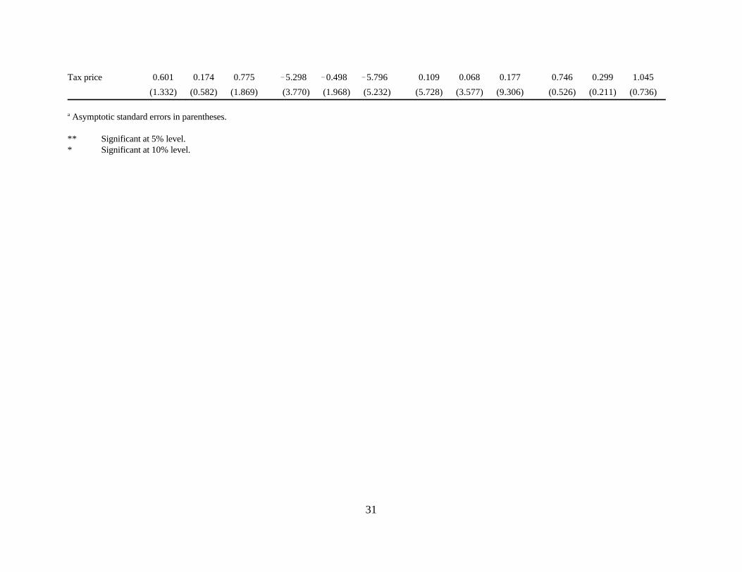
31

Tax price 0.601 0.174 0.775 5.298 0.498 5.796 0.109 0.068 0.177 0.746 0.299 1.045

(1.332) (0.582) (1.869) (3.770) (1.968) (5.232) (5.728) (3.577) (9.306) (0.526) (0.211) (0.736)

Asymptotic standard errors in parentheses.a

** Significant at 5% level.* Significant at 10% level.

32

Table 5. Elasticities of Binary Variables

Low-income Medium-income High-income Full sample

Variable Prob. level level Prob. level level Prob. level level Prob. level levelCond. Uncond. Cond. Uncond. Cond. Uncond. Cond. Uncond.

Some interest 0.054 0.504 0.215 0.037 0.640 0.235 0.078 1.006 0.836 0.148 1.681 0.918

Rural 0.032 0.482 0.152 0.024 0.263 0.075 0.040 0.533 0.459 0.011 0.130 0.080

Male 0.033 0.780 0.190 0.000 0.418 0.052 0.042 0.584 0.512 0.023 0.263 0.165

Head 0.001 0.152 0.010 0.016 0.254 0.104 0.039 0.536 0.470 0.002 0.018 0.011

Alberta 0.016 0.003 0.053 0.050 0.964 0.362 0.029 0.396 0.346 0.060 0.663 0.433

Manitoba 0.012 0.043 0.039 0.037 0.826 0.289 0.043 0.586 0.508 0.046 0.507 0.337

33

Table 6. Estimated aggregate reductions in donations to wildlife conservation in prairie Canada given 15% declines in income, hunting days andexpenditures on fish and wildlife recreation

Factor reduced Full sample modelIncome strata

Low Income Model Medium income model High income model

Income NS $2,350,000 $4,740,000 $4,700,000a

Days Hunting NS $540,000 $76,000 NS

Total Expenditures $17,000 $25,000 $180,000 $154,000

NS indicates that the elasticity was statistically insignificant and thus the reduction would not affect donation behaviora