1

Running Head:

San Francisco Bay Methylmercury Mass Budget

Corresponding author:

Donald Yee

San Francisco Estuary Institute

7770 Pardee Lane 2nd Floor

Oakland, CA 94621-1424

Tel:(510)746-7334 Fax:(510)746-7300

donald@sfei.org

2

Title:

A Simple Mass Budget of Methylmercury in San Francisco Bay, California

Authors:

Donald Yee

Lester J. McKee

John J. Oram

Address (for all):

San Francisco Estuary Institute

7770 Pardee Lane 2nd Floor

Oakland, CA 94621-1424

3

author email:

donald@sfei.org

4

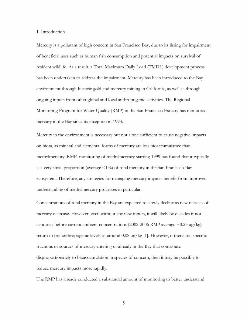
Abstract

San Francisco Bay is a water body listed as impaired due to mercury contamination in sport

fish for human consumption, as well as possible effects on resident wildlife. A legacy of

mercury mining in local watersheds and mercury used in gold mining in the Sierra Nevada

have contributed to contamination seen in the Bay, with additional more recent and ongoing

inputs from various sources. Even without continued mercury inputs, it would likely be

decades or centuries before ambient mercury concentrations return to pre-industrial levels.

Methylmercury is the species of mercury most directly responsible for contamination in

biota, so better understanding of its sources, loads, and processes was sought to identify the

best means to reduce impacts. A simple one box model of San Francisco Bay was applied to

evaluate uncertainties in estimates for methylmercury loading pathways and environmental

processes, to identify major data gaps, and test various management scenarios for reducing

methylmercury contamination. External loading pathways considered in the mass budget

include methylmercury loads entering via atmospheric deposition to the Bay surface, and

discharges from the Sacramento/San Joaquin Delta, local watersheds, industrial and

municipal wastewater, and fringing wetlands. Internal processes considered include exchange

between bed and suspended sediments and the water column, in-situ production and

degradation, and losses via hydrologic transport to the Pacific Ocean. In situ sediment

methylation and demethylation rates were dominant sources and losses determining mass

budget steady state concentrations, with changes in external loads and export causing smaller

changes. Better information on methylation and demethylation rates are thus most critical to

improving methylmercury budgets and management.

5

1. Introduction

Mercury is a pollutant of high concern in San Francisco Bay, due to its listing for impairment

of beneficial uses such as human fish consumption and potential impacts on survival of

resident wildlife. As a result, a Total Maximum Daily Load (TMDL) development process

has been undertaken to address the impairment. Mercury has been introduced to the Bay

environment through historic gold and mercury mining in California, as well as through

ongoing inputs from other global and local anthropogenic activities. The Regional

Monitoring Program for Water Quality (RMP) in the San Francisco Estuary has monitored

mercury in the Bay since its inception in 1993.

Mercury in the environment is necessary but not alone sufficient to cause negative impacts

on biota, as mineral and elemental forms of mercury are less bioaccumulative than

methylmercury. RMP monitoring of methylmercury starting 1999 has found that it typically

is a very small proportion (average <1%) of total mercury in the San Francisco Bay

ecosystem. Therefore, any strategies for managing mercury impacts benefit from improved

understanding of methylmercury processes in particular.

Concentrations of total mercury in the Bay are expected to slowly decline as new releases of

mercury decrease. However, even without any new inputs, it will likely be decades if not

centuries before current ambient concentrations (2002-2006 RMP average ~0.23 µg/kg)

return to pre-anthropogenic levels of around 0.08 µg/kg [1]. However, if there are specific

fractions or sources of mercury entering or already in the Bay that contribute

disproportionately to bioaccumulation in species of concern, then it may be possible to

reduce mercury impacts more rapidly.

The RMP has already conducted a substantial amount of monitoring to better understand

6

distributions, loads, and exposure of mercury and methylmercury, with more information

collection planned. Objectives of this mass budget exercise were to 1) collate information on

methylmercury distributions in the urbanized San Francisco estuary; 2) estimate

methylmercury loads from various pathways including atmospheric deposition, urban

stormwater, Delta outflow, wetlands, municipal wastewater, and other discharges; 3) develop

an annually averaged one-box mass balance for San Francisco Bay using empirical data on

local processes where possible and data for other regions in the literature otherwise. This

was a first step towards developing a better understanding of the factors most likely

controlling methylmercury concentrations on a Bay-wide scale. Much of the available

information was from intensive studies with limited temporal and spatial distribution, so

potential pitfalls of a simplified one-box mass budget include: 1) extrapolation of limited

data to wider temporal and spatial scales than appropriate, and 2) under-interpretation of

finer details of spatial and temporal data critical to local processes. These limitations will be

discussed and could be addressed in future work.

2. Methods

2.1 Location and Physiography

San Francisco Bay, California, USA, receives water, sediments and pollutants from local

watersheds, as well as from the Sacramento/San Joaquin River watershed (commonly called

the Central Valley), which covers an area of 154,000 km2 (~37% of California). Local

watersheds account for an additional 6,650 km2 , with a mix of urban (35% of the land area),

agricultural, and open space (e.g. park and other undeveloped) land uses. The volume of San

Francisco Bay is approximately 5.5 km3 with a surface area of 1,100 km2 at mean sea level. In

addition, a discontinuous fringing marsh of 950 km2 (greatly reduced from its historical

extent) occupies the area between uplands and the open Bay. Tides in the Bay are semi-

7

diurnal with a range (MLLW to MHHW) of 1.78 m at the Golden Gate Bridge, varying in

magnitude in various parts of the Bay. Average water discharge for the period 1971-2000

from the Sacramento/San Joaquin watershed past Mallard Island was 24.9 km3 annually [2].

Another 1.05 km3 of freshwater input is provided by the local watershed drainages.

Suspended sediment loads entering the Bay from the Delta average 1 billion kg/year [2].

There is no recent estimate of suspended sediment loads from local tributaries; the latest

best estimate was 0.75 billion kg/year [3]. The nine-county Bay Area population reached 6.78

million in the 2000 U.S. Census, growing at a rate of about 5% a year

(http://www.abag.ca.gov/planning/currentfcst/proj07.html), with another 6 million people

in the Central Valley, upstream of Mallard Island. Some of the larger industrial facilities in

the Bay area include oil refineries, a cement plant, an automobile plant, steel manufacturing

and fabrication, and computer and electronics manufacturers.

2.2 Environmental Monitoring

The Regional Monitoring Program (RMP) for Water Quality in the San Francisco Estuary

has conducted annual monitoring of open water areas in San Francisco Bay since 1993.

Additionally, RMP has conducted pilot and special studies examining pollutant

concentrations and loads entering the Bay by a variety of pathways at various locations.

Other projects and programs have monitored other locations and ecosystem components,

information useful in building our understanding of methylmercury processes in San

Francisco Bay.

Bay Ambient Water and Sediment

Although the RMP has been monitoring mercury in the Bay since its inception in 1993,

methylmercury measurements in water and surface (0-5cm) sediment have only been

8

included since 1999. Samples were collected during the dry season (summer) at fixed

locations from 1999 to 2001, and primarily at probabilistic sites with some fixed locations

since 2002. Historical fixed locations were located along a transect primarily following the

deep channel spine of the Bay. A Generalized Random Tessellation Stratified design used by

the U.S. EPA’s Environmental Monitoring and Assessment Program was applied to select

spatially unbiased probabilistic sampling locations locally [4]. Water was collected via

peristaltic pump from ~1m depth as either total (unfiltered) or dissolved (filtered, 0.45 µm

nominal pore size) samples and frozen in the field. Sediment samples were collected using a

modified Van Veen grab sampler, with surface (top 5 cm) sediments composited in the field

and immediately frozen.

Sacramento – San Joaquin River Delta

A methylmercury Total Maximum Daily Load (TMDL) report for the Delta [5] by the

Central Valley Regional Water Quality Control Board (RWQCB) estimated net

methylmercury exported from the Delta to the San Francisco Bay. In the Central Valley

TMDL, a major export site of water from the Delta is through the channel cross section

adjacent to Mallard Island, roughly the boundary of the Central Valley and San Francisco

Bay RWQCB jurisdictions. To obtain export load estimates, methylmercury concentrations

were measured at X2, the location in the estuary with 2 o/oo bottom salinity (which ranges up

to ~10 miles upland or seaward of Mallard Island), or at Mallard Island in more recent

studies. For the TMDL, Central Valley RWQCB staff monitored aqueous methylmercury at

X2 monthly from March 2000 to September 2001 and from April to September 2003.

Concentrations at Mallard Island were measured in a subsequent CALFED study. Net daily

Delta outflow water volumes were determined by the DAYFLOW model

(http://www.iep.ca.gov/dayflow/index.html).

9

Local Watersheds

A number of local tributaries with a mix of urban and other land uses have been monitored

by the RMP for total mercury and other pollutants, starting with monitoring of the mining

contaminated Guadalupe River in Water Year 2003, continued with a mix of funding

through to Water Year 2006. The Guadalupe River watershed area below reservoirs is 236

km2, with 13% industrial, 13% commercial and 58% residential land use. Sampling began at a

Hayward storm drain in Water Year 2007. Hayward Zone 4 Line A was selected for

monitoring in recognition that the Guadalupe River watershed is not representative of the

smaller urban drainages on the Bay margin which have no mercury mines, are more heavily

industrialized, and have almost 100% urban land use designation. Samples typically were

collected over the course of storm events and on a few occasions during base flow.

Concentrations in Guadalupe River and Zone 4 Line A have been reported previously [6-9].

Few to no measurements have been taken for other local watersheds, so estimates of

combined watershed loads for the region are made by extrapolation of methylmercury

percentage from these watersheds and regional estimates for mercury loading, with high

uncertainty given likely differences in watershed characteristics and mercury sources.

Municipal Wastewater

The San Francisco Bay RWQCB recently requested information on methylmercury

concentrations from local municipal wastewater dischargers over the course of a year (2007-

2008). Using clean techniques, dischargers collected monthly effluent grab samples and

reported discrete and annually-averaged concentrations. These average concentrations were

combined with annual discharge rates for each of the plants to estimate annual

methylmercury loads. The reporting municipal dischargers account for 95% of the regional

effluent discharge.

10

Wetland concentrations

Concentrations of methylmercury in wetland waters have been reported in a number of

studies. Studies in wetlands of the North Bay (e.g., Petaluma Marsh [10]; Suisun Marsh [11]),

have reported water column concentrations on incoming and outgoing tides for specific

events, but comprehensive monitoring across many days over spring/neap cycles in multiple

seasons has not been performed due to the large field and laboratory effort this would entail.

Data on water column concentration differences between incoming and outgoing tides

measured in the Petaluma study, and estimates of leachable methylmercury produced in the

Hamilton Army Air Field wetland [12] can be used to provide an estimate of wetland

methylmercury discharge, albeit with large uncertainties. However, such first order estimates

based on existing information could indicate whether wetland discharges are a potential

source of concern given the range of concentrations and loads in the sparse data found thus

far.

2.3 Mass Budget Model

A one-box model of water and sediment processes was employed to integrate existing

monitoring efforts and to enhance our understanding of methylmercury fate in San

Francisco Bay. The model was initially developed by Davis [13] to predict the long-term fate

of PCBs in San Francisco Bay and has been used for developing mass budgets for PAHs,

organochlorine pesticides, and PBDEs [14-16]. The one-box model of San Francisco Bay

treats the Bay as two well-mixed compartments representing the water column and surface

sediments. Conceptually, the model ignores differences in the geographic sub-regions of the

Bay, a simplification that precludes deeper understanding of temporal and spatial variations,

but allows a first-order evaluation of the system. The model includes parameters for

describing major physical and chemical processes governing the transport and fate of

11

contaminants in the system. These processes include:

1. external loads,

2. settling and resuspension of sediment particles,

3. water-solid partitioning (sorption/desorption),

4. sediment-water diffusive exchange,

5. volatilization,

6. degradation in water and sediment,

7. tidal flushing and outflow, and

8. in-situ production.

In-situ production is a major component missing from the earlier one-box models, as it is

negligible for the previously modeled organic contaminants but is critical for methylmercury

given its facile transformation to and from inorganic forms. A previous effort for a mass

balance of mercury in the San Francisco Bay treated these transformations as a pseudo-

equilibrium characteristic, using a fixed percentage of total mercury [17] to model a pseudo-

steady state methylmercury concentration. However, in this model we do not attempt to

express methylmercury as a function of total mercury concentration. Instead, methylmercury

production is treated as a specified (input) rate in a methylating zone of sediment. A rate

calculated based on total mercury would effectively have been a specified methylmercury

input rate, unless it was linked to a concurrent model of long-term large change in total

mercury mass balance.

2.3.1 Model External Loads

In the model, some inputs to the Bay are external and not dependent on concentrations in

the Bay; these include inputs entering from the air via direct deposition or from the land via

rivers, tributaries, channels, and discharge pipes. External loads are discussed below, and

12

summarized in Table 1. Although flows and loads (e.g. from precipitation runoff in the Delta

and local watersheds) are not uniform over the course of the year or evenly distributed in

space, this model simplifies temporal loads by treating inputs as occurring uniformly

throughout the year and simplifies spatial heterogeneity by assuming all loads enter the Bay

evenly spatially (one well-mixed box). These simplifications are important to the system

response and will be discussed in detail later.

Sacramento – San Joaquin River Delta

In the Delta methylmercury TMDL [5], average annual methylmercury exports were

estimated for water years (WY) 2000 to 2003 (relatively dry years). Concentration data for

samples collected at X2 from two sampling periods (March 2000 to September 2001, and

April to September 2003) were combined to derive monthly average concentrations, and the

DAYFLOW program was used to derive average monthly flows. Methylmercury

concentrations at X2 ranged from below detection limits to 0.241 ng/L, averaging 0.075

ng/L over all periods combined. Monthly average concentrations were multiplied by

monthly average flows for WY2000-2003 to estimate monthly loads. Monthly loads were

summed to calculate an annual average methylmercury load of 1.7 kg/year (4.7 g/day). A

simple model regressing Delta outflow to methylmercury concentration for that period

resulted in a similar estimate, with export of 2.1 kg/year. Given their similarity, the monthly

average derived export was used in the TMDL mass balance.

A subsequent CALFED funded study measured methylmercury concentrations at both

Mallard Island and at X2 from October 2004 to November 2005 to examine differences

between estimated fluxes for the two locations, but no significant differences were found.

Combining previous data used in the TMDL with the new data resulted in an estimated

average export flux of 9.8 g/day, These export calculation sonly attempted to estimate

13

advective flux from the Delta, but dispersive flux could also affect net export. Ignoring

dispersive transport generally results in an overestimate of advective flux by around 15% for

periods of Delta outflow over 500 m3/s [2]. The error in estimated mercury advective flux

would be expected to be of a similar magnitude, but even with correction for dispersive flux,

temporal variability in annual flux is still larger (stdev ~30/% of average). Potential impacts

of all these uncertainties are later assessed together through sensitivity testing of the estimate

for Delta flux in combination with other external loads.

Local Watersheds

Concurrently collected samples were analyzed for methylmercury and total mercury in the

Guadalupe River and Hayward Zone 4 Line A watersheds for events in one or more rainy

seasons for RMP special studies of local watershed loads. Guadalupe River total (combined

dissolved and particulate phase) methylmercury concentrations ranged 0.05 to 2.2 ng/L

(average 0.7 ng/L), which was an average 0.45% of total mercury concentrations (0.05 to

1.9%). Total methylmercury concentrations in Hayward Zone 4 Line A samples ranged from

0.08 to 1.3 ng/L (average 0.44 ng/L, 1.6% of total mercury in water). Other urban sites

around San Jose had similar concentrations, with San Pedro Street storm drain ranging 0.02

to 3.1 ng/L (average 0.84 ng/L) , and 0.95 ng/L for a single sampling event at Airport

Parkway. Methylmercury was 0.43% and 1.4% of total mercury for those sites, respectively.

Because methylmercury concentrations and percentages (of total mercury) were not yet

known for other watersheds, estimates for the rest of the region required extrapolation of

the limited existing data. Methylmercury percentages in the literature ranged widely, although

percentages reported were generally below 10%. Thus the concentrations and percentages

found here in stormwater (methylmercury between 0.02 to 3 ng/L, averaging 0.4 to 1.5% of

total mercury, for various land use types) did not seem unreasonable. In RMP ambient

14

monitoring throughout the Bay, methylmercury averaged <1% of the total mercury in the

water column, and a similar percentage (average 0.7%) was found in the Delta to Central Bay

for another study [18]. A synoptic study of the upper portions of the Guadalupe River

watershed [19] also found similar distributions at the station furthest downstream (Los

Gatos Creek near its confluence with the Guadalupe River), with methylmercury 1.2% of

total mercury. Thus average methylmercury loads at around 1% of total mercury loads were

likely to be a reasonable first order estimate.

Total mercury loads at a regional scale have been estimated using multiple methods (e.g. the

SIMPLE model [20], or combining bed sediment concentrations with regional suspended

sediment loads estimates [21]). Regional total mercury loads estimates from these previous

studies ranged from 123 to 185 kg/year. The corresponding methylmercury loads based on

1% of total mercury loads would be between 1.2 to 1.9 kg/year.. Given uncertainties

associated with estimating methylmercury as a fixed percentage of total mercury described

previously, a second method was applied to provide a comparison. A first order estimate of

methylmercury can also be developed using the limited existing data for general land use

types and the SIMPLE model [22]. Mass loads of methylmercury estimated in this manner

were 1.3kg/year (0.4 kg/year for urban watersheds, 0.4 kg/year for non-urban watersheds,

and 0.5 kg/year from the Guadalupe River alone). Using the SIMPLE model to estimate

total mercury loads for different watershed types in the region and multiplying by average

methylmercury percentages for those land use types resulted in slightly (~3x) higher

methylmercury load estimates, with about 1.5 kg/year from urban watersheds, 1.3 kg/year

from non-urban areas, and 0.5 kg/year from the Guadalupe River. Summing these gives a

total estimated annual average methylmercury load entering the Bay of 3.3 kg/year. Given no

way to know which of the estimates was “better”, we elected to use a load between the two

15

described. Thus, a load of 2.3 kg/year was chosen as the default estimate of local watershed

loads for the mass budget exercise. Given the limited available data, there was substantial

uncertainty in the possible range of methylmercury concentrations and percentages. In

acknowledgement of this uncertainty, the mass balance model developed here was tested

over a one order-of-magnitude range of for local watershed loads.

Wastewater

Monthly methylmercury data from the 16 largest treatment plants were compiled, and

combined with data on mean annual discharge volume [23] to estimate mean annual

methymercury loads. These plants account for around 95% of wastewater discharged to the

Bay, yielding a total methylmercury load of 0.8 g/day. Concentrations at treatment plants

were highly variable (mean RSD ~65%), so testing an order of magnitude range of loads for

the model sensitivity runs would likely include the true load.

Wetland Discharge

Net import or export from tidal wetlands can be calculated from measured concentrations

and flows in the water column during flood and ebb tides. Neither currents nor

methylmercury concentrations are uniform over the course of a tidal cycle, and most

wetlands have multiple inlets and outlets, so many measurements at many locations would be

needed to get an accurate estimate of net transport for even a single wetland. Given the

paucity of data on net import or export for the numerous wetlands fringing the Bay,

simplifying assumptions and extrapolations were made to estimate export rates, which could

be compared to standing methylmercury inventories and production rates in wetlands to

determine their reasonableness.

The current extent of tidal marsh area in the San Francisco Bay region is about 40,000 acres,

greatly reduced from 190,000 acres historically, due to diking and infill [24]. These wetlands

16

vary widely in elevation, vegetation, and hydrological connectivity, but to simplify for this

mass budget exercise, we treated all these areas as similar. Long term tidal data for NOAA

benchmark stations around San Francisco Bay (Port Chicago, Mare Island, Richmond, San

Francisco, Alameda, Redwood City) show differences between mean high water (MHW) and

mean tide level (MTL) averaging 0.7 m. Assuming wetland areas have constant slopes, a tidal

prism with an average of 0.35 m water covers the marsh surface on each high tide (twice

daily), an equivalent depth of over 200m of water is transported on and off wetlands

annually. Local wetland evapotranspiration rates are estimated around 1m/year [25], and

average annual rainfall around 0.5m/year

(http://www.wrcc.dri.edu/summary/Climsmcca.html), so water movement via tides

swamps other hydrologic transport pathways in most tidal wetland areas. Although episodic

flows from storm events may transport greater volumes for short periods, on an annual

basis, transport via daily tidal flows likely dominate in wetland areas other than directly along

stream banks, areas already counted as tributary loads.

In a wetland near the mouth of the Petaluma River studied in a Calfed-funded project, water

column concentrations over 24 hours were monitored to obtain estimates of the net flux of

methylmercury [10]. Peak water column dissolved methylmercury concentrations on ebb tide

were up to ten times higher than concentrations seen during flood tide, with the average ebb

concentration (0.136 ng/L) almost double the average flood concentrations (0.083 ng/L). In

contrast, particulate concentrations averaged slightly higher during flood tide (0.098 ng/L)

compared to ebb tide (0.092 ng/L). Extrapolating the difference in dissolved methylmercury

between flood and ebb tides, with hydrologic transport primarily by approximately equal

volumes of tidal flows in and out of wetlands, methylmercury mass exported from 40,000

acres of tidal marshes around San Francisco Bay would total 6.0 g/day. Similarly, from the

17

difference in particulate methylmercury concentrations between incoming and outgoing

tides, about 0.7 g/day of methylmercury would be transported from the Bay to wetlands.

Thus net methylmercury transport would be 5.3 g/day exported from wetlands to the Bay.

In a study of the Hamilton Army Air Field (HAAF) wetland, the USACE [12] estimated

potential methylmercury export by another methodology. They assumed that solubility

would control methylmercury transferred from wetland sediments to overlying water. The

net methylmercury production rate was estimated to be 3.1 µg/m2/day at HAAF. Based on

mercury solubility [26], 0.4% of methylmercury was estimated to be exchangeable with the

water column. Combined with twice daily tides, 0.8% of daily net methylmercury production

would be removed through tidal transport. Extrapolating the HAAF rates to the total

wetland area around the Bay, 4.0 g/day of methylmercury would be discharged to the Bay

from wetlands. This export rate is of the same order-of-magnitude as that estimated by the

difference in flood and ebb tide concentrations at Petaluma.

Studies in Suisun Marsh [11] found mixed results in net methylmercury transport, with some

studied periods and locations showing net import to the marsh, and others showing net

export. Although dissolved and particulate methylmercury were not measured separately in

those studies, the authors hypothesized that differences in net transport resulted from

differences in hydrology and particulate and dissolved phase methylmercury between events

and locations. This is consistent with findings in the Petaluma wetland, with higher

particulate concentrations in flood tides and higher dissolved concentrations in ebb tides. An

accurate determination of net methylmercury transport between a wetland and the Bay

would require monitoring over a long term under a wider range of hydrologic conditions

(flood and ebb tides under spring and neap tide periods during wet and dry seasons,

including rainfall events of different intensities and durations), a task beyond the scope of

18

most studies, including this exercise. However, the rough estimates provided by studies

conducted to date provide a starting point to evaluate the relative importance of refining

wetland load estimates.

Atmospheric deposition

The majority of atmospheric mercury monitoring under the Mercury Deposition Network

measures only total mercury in wet deposition, although sites have occasionally monitored

methylmercury concentrations. Although an MDN station measuring total mercury was

maintained near San Jose for 6 years, methylmercury in precipitation was not measured at

that local station. The U.S. Geological Survey, in cooperation with the Indiana Department

of Environmental Management monitored both total and methyl mercury in precipitation at

several stations in Indiana between 2001 to 2003 [27]. For the 3-year period, the median

methylmercury concentration in weekly samples was 0.058 ng/L with a maximum of 5.77

ng/L. Methylmercury was also found in precipitation in a similar concentration range (0.01

to 0.179, average 0.052 ng/L) in the Experimental Lakes area of Northwestern Ontario [28].

Rain samples collected during a storm event passing over the North Olympic Peninsula in

western Washington State showed average methylmercury concentrations of 0.15 ng/L [29].

Taking the mean methylmercury concentrations in rainfall of these various studies, (0.087

ng/L) and applying San Francisco Bay area mean annual rainfall (typically between 0.4 to 0.5

m/year), direct wet methylmercury deposition to the Bay is estimated to be 0.1 g/day.

Methylmercury in dry deposition is seldom measured. A recent study characterized dry

deposition of methylmercury in Canada’s ELA through collection of throughfall and

litterfall, subtracting open field deposition [30]. Although it is possible to measure

throughfall and litterfall in surrounding watersheds, dry deposition of methylmercury onto

watersheds is already accounted for in the estimation of watershed loadings via tributaries.

19

The combined throughfall and litterfall deposition rates in the ELA study were up to double

the rates of wet deposition, so as a first-order approximation, any dry deposition directly to

the Bay would likely be a similar order-of-magnitude as wet deposition.

2.3.2 Model uptake loss to biota

Potential methylmercury bio-uptake was modeled as a loss, using biota for which relatively

good inventories exist to evaluate their impact on the overall mass budget. With sufficient

information methylmercury uptake into biota might eventually be modeled using

concentration dependent relationships. However, a lack of good inventories for many types

of biota and a lack of sufficiently detailed information on the relationship between various

biota and water or sediment concentrations precluded explicit modeling of these processes

for the mass balance developed here.

Estimating uptake of methylmercury by primary producers would be a possible starting

point towards quantifying bio-uptake of methylmercury, but the rapid turnover rate of

phytoplankton (0.2-0.7/day [31]) suggests that much of the methylmercury in phytoplankton

could be rapidly cycled, with a large fraction returning to the water column and sediment.

That fraction recycled would depend on what proportion of phytoplankton was consumed

by higher tropic organisms and the methylmercury assimilation efficiency of those biota.

Because the primary interest of this exercise was to model the fate of methylmercury on

annual and interannual time scales, small fish seemed reasonable candidates for estimating

annual methylmercury transfer to biota. Small fish are relatively well studied in the Estuary,

with the California Department of Fish and Game conducting monthly trawls in the Bay and

Delta for the California Department of Water Resources Interagency Ecological Program

(I.E.P). The size/age relationship for various species in the Bay have been studied, so the

mercury body burden in the young-of-year cohort was used to represent annual-scale net

20

uptake.

The mean pelagic fish biomass in June-October trawls for areas in northern San Francisco

Bay in the intermediate and high salinity areas typically ranged 100 to 1000 g carbon (g C)

per 10,000 m3 trawled [32]. Using the geometric mean of the year 2000 to 2006 range (~0.02

to 0.03 g C/m3), and converting back into wet weight (original data were expressed as wet

weight catch per unit effort), we found about 0.17 g/m3 in (pelagic) young-of-year fish

biomass. The average mercury wet weight concentration in small fish measured in San

Francisco Bay by the RMP was 0.049 µg/g. Applying the young-of-year fish density to the

total Bay volume, assuming the uptake rate is uniform over the course of a year, an estimated

0.13 g/day of methylmercury is transferred to small fish biomass each day. The data from

mid-water trawls likely under-represented benthic residing fish. However, the mercury mass

estimate also likely overestimated pelagic fish in deep waters by applying their density to the

entire Bay water volume.

Subsequent otter (bottom) trawl data supplied by CDFG (Steven Slater, CDFG, Stockton,

CA, personal communication) suggested these errors roughly offset. Combining all the Bay

segments for 2000 to 2006 resulted in a wet weight average 0.21 g/m3 for demersal fish

density. Thus the estimated net biouptake loss of methylmercury to fish likely was of the

right order of magnitude and was a very small component (~0.5%) of overall methylmercury

loads to the Bay.

This fish biomass estimate might also have been spatially biased as the mid-water trawls only

sampled water 2.5 m or deeper. The US Fish and Wildlife Service conducts beach seining in

waters up to ~1m deep as part of the Delta Juvenile Fish Monitoring Program

(http://www.fws.gov/stockton/jfmp/monitoring.asp). Biomass catch per unit effort in that

program was about ten-fold higher than in the open-water trawls (around 2 g/m3 ) but

21

waters <2.5 m deep account for around one tenth of the Bay volume. Including the beach

seine data to derive a volume weighted average biomass would thus only double the amount

of methylmercury to biomass (to ~1% of external methylmercury loads).

2.3.3 Model Internal Process Estimates

A majority of the Bay internal processes in the one-box model were dependant on ambient

concentrations in Bay waters and sediments. Degradation was modeled as a first order

reaction proportional to methylmercury concentration in the modeled compartment. For

transport and partitioning, relative concentrations between water and sediment and adjoining

compartments such as the Pacific Ocean and the atmosphere were needed. Many of the key

model parameters are listed in Table 2 and discussed below.

Atmospheric volatilization

Methylmercury can volatilize as the charge neutral species MeHgCl. Air-water partitioning of

MeHgCl was measured for 0.7 M NaCl [33] with a dimensionless Henry’s law constant of

~2×10−5 at 25 °C. The volatilization rate calculated by the model using this constant was

likely biased high, as the Bay water surface temperature is below 25 °C for most of the year.

Furthermore, not all the “dissolved” phase methylmercury in surface waters is present as

MeHgCl, as methylmercury may also complex with dissolved organic matter or partition to

colloidal material in the operationally defined (<0.45 µm) “dissolved” phase. Binding

constants with humic acids in freshwater [34] and gel permeation chromatography [35]

suggest that half or more of dissolved methylmercury may be complexed to various forms of

DOC. Heavy organically complexed and adsorbed colloidal methylmercury are not volatile,

so given dissolved methylmercury concentrations are only partially MeHgCl or similarly light

charge-neutral species, the rate of volatilization calculated from literature constants [36]

represents an upper bound estimate of the loss rate by this pathway.

22

Degradation in water and sediment

Degradation in the sediment and the water column was modeled as an internal loss pathway

for methylmercury. Degradation can occur through a number of biotic and abiotic pathways.

In San Pablo Bay sediment, oxidative demethylation was posited to be a primary mode of

degradation based on the by-products of 14C-methylmercury demethylation experiments [37].

Sediment first-order degradation rate constants ranged from 0.019 to 0.25 /day (i.e. 1.9 to

25% of methylmercury degraded per day) in that study. We applied the geometric mean

(0.083 /day) as the rate constant for sediments throughout the Bay. Most degradation rates

in the San Pablo Bay study were determined for surface (0-4 cm depth) samples, but in the

one site where degradation rates were measured at multiple depths (8 cm and deeper),

degradation rates were up to about 10-fold lower below 8 cm. Therefore for purposes of the

mass balance model, we assumed that sediment methylmercury degradation primarily

occurred in the top 7 cm of sediment, with negligible degradation in the deeper anoxic

layers.

Methylmercury degradation in the water column also may occur through biotic pathways

similar to those in sediments, but abiotic pathways such as photodemethylation are the focus

of most degradation studies in surface waters. Degradation rate constants of 0.11 to 0.22

/day were measured in Delta surface waters [38]. Similar rates were seen in photo-irradiated

water samples from Petaluma wetlands, with half-lives of 5 to 20 days for filtered waters, and

generally longer half-lives (11 to 20 days) for unfiltered waters. Petaluma samples nearest San

Pablo Bay had the shortest half-lives in filtered samples of 5 to 6 days, but wetland waters

are much shallower than those in most areas of the Bay (typically 1 m maximum depth at

high slack tide compared to the Bay average of around 5 m).

Waters at shallow depths typically experience higher levels of irradiation and thus show

23

higher rates of photodemethylation [39]. Shallow Bay surface waters are likely to have a

demethylation half-life similar to that seen in the wetland nearest San Pablo Bay of 7 days

(first order degradation rate of approximately 0.1 /day). Unlike in the wetlands however,

light penetration in much of the Bay is not likely to extend the entire depth of the water

column to the sediment surface. Light penetration in northern San Francisco Bay as

measured by Secchi disk in three segments (Suisun, San Pablo, and Central Bay) over four

seasons, ranged 0.3 to1.6 m [40]. In all but 2 measurements (Central and San Pablo Bay in

the fall), average Secchi depths were 1.1 m or shallower. Thus, assuming that demethylation

occurs only over the top ~1 m of surface waters, the demethylation rate applied to the entire

water column was modeled as being five-fold lower (0.02 /day).

Tidal flushing and outflow

Bay-specific model parameters were identicaltothoseusedinpredictingthelong‐term

fateofPCBsintheBay[13],withtheadditionofatidalflushingratio(α=3.75),

whichistheratiooftidalexchangeflowtonetfreshwaterflowinthesystem.Tidal

flushingwasnotincludedintheoriginal application of the one-box model to PCBs, but

was added to the one-box model in response to review comments [41] and used in more

recent applications of the one-box model such as the PBDE mass balance [16].

Methylmercury concentrations in the water column measured by the RMP at the Golden

Gate station outside of San Francisco Bay typically have not been detected (<20 pg/L). For

the base case assumption running the one-box model, ocean waters were assumed to have

no methylmercury (concentration of 0 pg/L), which would maximize the estimated net

export rate, as methylmercury would only be transported with the ebbing tide, transporting

methylmercury from the Bay to the ocean. The model was also tested using different oceanic

methylmercury concentrations to assess the sensitivity to this assumption.

24

Sediment-water partitioning

Partitioning of methylmercury between the water and sediment phases is an important

characteristic of the system. The sediment-water partition coefficient (Kd) determines the

degree to which methylmercury in sediments adsorb to or desorb from particle surfaces.

Methylmercury loads introduced via the water column may adsorb to suspended particles

and settle to the sediment bed. Conversely, methylmercury produced in sediment may

dissolve from bed sediments into porewater or desorb from resuspended particles into the

water column. The partition coefficient is treated as the equilibrium ratio (L/kg) between

concentrations in solid (µg/kg) and liquid (µg/L) phases. The use of partition coefficients

relies on the assumptions that the kinetics of partitioning are fast relative to other processes;

for example, the Kd would become elevated as the apparent water column concentration

were decreased by biological degradation or hydrologic exchange that removed

methylmercury much faster than it could be replenished by desorption.

Kinetics of methylmercury adsorption and desorption are relatively fast, reaching equilibrium

on the order of hours [42], compared to the model daily time step, hydrologic turnover times

on the order of a week or greater, and the annual or longer time scale scenarios being

modeled. Thus although equilibrium assumptions may not be strictly correct, they were

reasonable approximations of partitioning in the system for the one-box model. Using the

Bay-wide mean particulate methylmercury concentration in water (49.6 pg/L), the Bay-wide

mean dissolved methylmercury concentration in water (44.5 pg/L), and the Bay-wide mean

concentration of suspended particles in water (0.085 g/L), the methylmercury partitioning

coefficient was estimated to be 13,100 L/kg (log Kd=4.11), consistent with other

measurements in the San Francisco Estuary [43] and similar to that reported for the

Guadalupe River [8]. If instead the average bed sediment methylmercury concentration

25

(0.558 µg/kg) was used, the resultant Kd between sediment and the water column was

12,500 (log Kd = 4.09), virtually the same. A value of 13,100 L/kg was used as the water

column Kd for the base case in the model, with higher and lower partition coefficients used

for sensitivity analysis.

The partitioning of methylmercury in sediment porewater may potentially differ from that in

overlying water column due to differences in various factors that affect its solubility such as

organic carbon concentrations and sulfide speciation. Work in northern San Francisco Bay

[18] examined sediment and porewater concentrations of methylmercury and derived Kd for

those sites (log Kd = 4.7 ± 0.4 (average ± stdev)). This translates to a mean porewater Kd of

45,700, about the same order-of-magnitude as the partition coefficient for the water column

as estimated above. A porewater Kd of 45,700 (log Kd = 4.7) was used for the base case

model scenario. Effects of higher and lower porewater Kd were tested during sensitivity

analysis.

Sediment-water column particle exchange

The exchange of particles between the water column and the bed sediment of the Bay is not

spatially uniform and highly dependant on many environmental factors, such as tidal

currents, water depth, wind waves, and particle export from local watersheds and the Delta.

The one box mass balance model did not capture such spatial heterogeneity, and given its

simplifying assumptions it is best suited to simulating a simple system achieving a long-term

pseudo-steady state condition, rather than dynamically modeling episodic or transient events.

Although the simplifying assumptions of uniform mixing and equilibrium were not accurate

synoptic representations of the system at any particular time, in the longer term, the system

tends to range around a mean, which might be reasonably modeled as a steady state

condition so long as the kinetics of the modeled processes are much shorter than the

26

modeled period. The similarities in suspended sediment and bed surface sediment

partitioning constants suggest that a model of continuous exchange between these two

compartments is reasonable.

One major simplification was the treatment of suspended sediment concentration as

approximately constant. Although there has been a long-term trend toward reduced

sediment loads coming from the Delta in recent decades [44, 45], given the high turnover

rate of other modeled processes compared to the long-term change in SSC, modeling of

water-sediment particle exchange was simplified and treated as a steady state (i.e. all inputs

roughly equal all losses). Another major simplification is the treatment of the mixed

sediment layer as a uniformly mixed compartment. In the case of conservative pollutants, a

uniform mixing assumption tends to accelerate the response of the system to changes in

loads, as increases or reductions in loads will be modeled as occurring instantly equally

throughout the Bay. However, methylmercury is not a conservative pollutant; given turnover

times on the order of days for some processes such as degradation, the impacts of an

instantaneous mixing assumption are lessened. Although the system response time to

changes will be shortened by the uniform mixing assumption, the resulting steady state mass

achieved should be essentially the same in the long term.

Sediment-Water Column Porewater Exchange

In addition to exchange of particulate matter between the sediment and water column,

exchange of porewater with overlying water is another pathway for methylmercury transport.

Porewater exchange can occur through abiotic processes such as diffusion or resuspension

by wind-wave processes, or through biologically mediated processes, such as bioirrigatation

and bioturbation by benthic organisms. Flux rates may be empirically determined via flux

box measurements or through mesocosm experiments, although each approach presents

27

limitations which may lead to differences in net flux from in-situ conditions. For example,

mesocosms, even if transferred intact, are disconnected from the larger ecosystem and thus

may not entirely reflect native conditions. Unless processes such as wind-wave and tidal

current shear stresses, tidal pumping, and groundwater flow are adequately simulated, those

components of transport will not be included. Similarly, flux box experiments, although

maintaining some connection with the surrounding system, tend to isolate the studied patch

from waves and currents, and may trap or exclude mobile macrofauna, leading to

unrepresentative rate measurements.

Nonetheless, in-situ flux box experiments likely represent the best available measurement of

actual fluxes in the native ecosystem, and provide a reasonable likely lower bound estimate

of net flux due to possible exclusion of some abiotic forces such as resuspension by waves

and stronger currents. Flux measurements were made in benthic chamber deployments in

Suisun Bay and the Delta [18]. The benthic chambers were “gently stirred”, which reduced

the boundary layer at the sediment-water interface, but likely were not sufficient to

resuspend bed sediments. The median flux rate measured was 13 ng/m2/day (10 to 90th

percentile range 2 to 55 ng/m2/day). Applying that flux rate to the Bay surface results in a

net flux of 14 g/day. However, the Bay average concentration differences in porewater and

overlying water may not be the same as in that work., so concentrations and measured fluxes

were combined to estimate a transfer velocity (Vd) applied in the form:

Flux (ng/m2/day) = Vd (m/day) * [Csed –Cwater] (ng/m3)

where Csed and Cwater are dissolved methylmercury concentrations in the sediment

porewater and overlying water, respectively. The resultant estimated Vd was 0.001 m/day,

which was used to parameterize the one-box model.

Although they did not measure methylmercury flux, the U.S. Geological Survey measured

28

total mercury flux in a number of South Bay sites [46]. Average dissolved mercury fluxes

ranged from 100-400 ng/m2/day. Assuming porewater ratios of methylmercury:mercury

similar to those for the sediment (~1% or less), corresponding methylmercury fluxes would

be around 1 to 4 ng/m2/day, about the same range as found in the North Bay/Delta study

of Choe et al. This provides another estimate for methylmercury flux and additional

verification that the parameters for estimating benthic flux are reasonable when considered

in the larger context of other available data for the Bay.

Sediment burial or erosion

Net burial or erosion of bed sediments could also result in methylmercury loads to or losses

from the mixed sediment layer. In part due to the relatively rapid sediment degradation rates

noted previously, methylmercury concentrations found at depth measured in samples from

this region were lower than those in surface samples [37]. Thus unlike the persistent organic

pollutants such as PCBs and the inorganic metal pollutants such as mercury or copper, there

are not likely to be substantial deeper legacy deposits of methylmercury with higher

concentrations that can become exposed through erosion and re-introduced into the

ecosystem.

Net sedimentation leading to burial of below the active sediment layer can remove

methylmercury from exposure to biota. The average net sedimentation rate of 0.83 cm/year

for a core taken from Richardson Bay in 1992 [47] would indicate that less than 10% of the

methylmercury inventory in the 10cm mixed sediment layer of the one-box model would be

lost by burial each year. Another core in that study from San Pablo Bay suggested a much

higher burial rate, averaging 4 cm/year. However, comparisons of bathymetric change

suggest that such high burial rates are atypical for much of the Bay [48-50], with most areas

showing no net bathymetric change or slight erosion (typically <0.5 m in 30-40 years) in

29

recent history. However, even assuming such high rates were widespread, burial losses of

40% of the methylmercury in surface sediments over a year are likely dwarfed by potential

losses of a similar magnitude in just a week via degradation in sediments. The model

response to changes in the burial rate and other assumptions are discussed below.

3. Results and Discussion

3.1. Model Hindcast

Like the PCB and PBDE mass budget models [13, 16], the methylmercury mass budget was

run in both hindcast and forecast modes. A hindcast is most useful when there is sufficient

data to parameterize the model historically, and the modeled pollutant is sufficiently

persistent that prior condition is a significant factor in determining the current state of the

system. Unlike for PCBs or PBDEs, little or no information exists regarding the history of

likely changes in global or local emissions and loading rates for methylmercury, nor of large

changes in partitioning, production, degradation or other processes. Thus, the hindcast

scenario was identical to the forecast aside from the initial condition. The sensitivity of the

model to historical conditions was tested by adjusting the initial ambient concentrations.

Current loading and process rates in the model have no linkage to the historical rates other

than through their dependence on ambient concentrations. In the hindcast, to bound the

possibilities given no knowledge of the prior condition, we either assumed that ambient

methylmercury concentrations in water and sediment were zero, or that they were an order

of magnitude (10 times) higher than the current condition.

The zero initial concentration condition represented the hindcast best case scenario,

essentially assuming that prior to any anthropogenic mercury releases, ambient

methylmercury inventories were negligible. The model was run for two years with

continuous loading rates and internal processes using contemporary rates and coefficients

30

until a steady-state methylmercury mass was achieved. The modeled system reached steady-

state quickly, stabilizing within <100 days. The opposite case, with the initial condition set at

10 times the current ambient inventory, quickly reached the same equilibrium within <100

days. This indicated that prior condition had negligible influence on determining the

methylmercury steady-state inventory of the modeled Bay system.

3.2 Base Case Forecast

As stated previously, no data exist indicating significant changes in rates and coefficients for

various processes. Thus, the same rates and coefficients for these parameters were used in

the model hindcast and forecast. In forecast mode, the model was initialized with the best

estimate of the current methylmercury mass in the Bay and external loads of between 2.7

and 24 kg/yr (from 1/3 to 3 times the base case) were examined. Given the same final

steady state under both the low and high concentration initial condition assumptions in the

hindcast runs, not surprisingly, the base case scenario quickly arrived at a steady state with

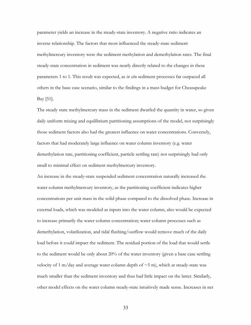
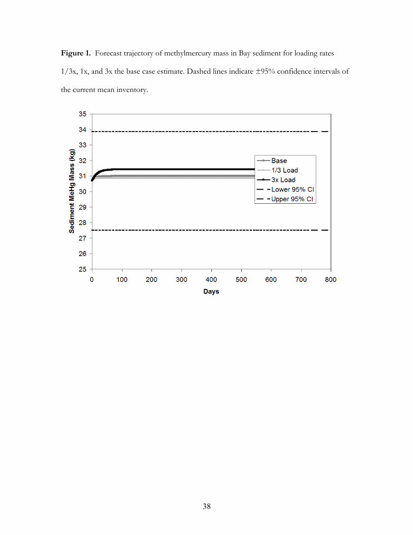
the same final inventory (Figure 1). Varying loading rates over nearly an order of magnitude

(9x) range had little effect, with the sediment inventory virtually unchanged, and projected

water inventories almost within the 95% confidence interval of the current mean of RMP

ambient measurements (Figure 2).

The magnitudes of various methylmercury environmental loading and process rates (kg/day)

are listed along with the base case steady state inventory (kg) in Table 3. For the sediment,

methylation and demethylation respectively produce and remove nearly 6% of the Bay

sediment methylmercury inventory each day. Net methylmercury removed by sediment

accretion leading to net burial, was next largest but only 0.007 kg/day, around 250 times

smaller. Sediment exchange with the water column was a similar magnitude, 0.007 kg/day.

The net exchange was mostly the result of water column suspended particle settling (0.038

31

kg/day methylmercury) combined with bed sediment resuspension (0.045 kg/day

methylmercury). Masses of sediment settling out and resuspended to the water column each

day were roughly equal in the base case, so the differences in downward versus upward flux

were primarily due to differences in methylmercury concentrations of suspended versus bed

sediments.

For methylmercury in the water column, the largest inputs were external loads (including

atmospheric deposition, Delta, local tributary, wastewater, and wetlands discharge), and

exchange with the bed sediment, which were of roughly the same magnitude in the base

case. At steady-state, these inputs were nearly offset by degradation in the water column and

outflow from the Bay, which were also of similar magnitudes. The other loss pathways

included, biouptake into fish and volatilization of methylmercury, were so small as to be

negligible in the mass budget.

Although the Bay is not truly a steady-state system, gross deviances in the model steady-state

from the initial condition (derived using mean concentrations) would suggest major errors or

uncertainties in some of the model parameters and/or assumptions. For the sediment, the

model methylmercury inventory at the final steady state (30.8 kg) was similar to the initial

ambient condition inventory set using averaged RMP monitoring data (30.7 kg). Given that

the initial inventory had little influence on the final steady state, the slightly higher final

inventory suggested small errors or uncertainties in some model parameters. The direction of

difference suggested are errors that introduced too much loading and/or production in

sediment, or yielded too little removal and/or degradation.

However, in contrast to the approximately constant sediment inventory in the base case

forecast, the base case methylmercury inventory in the water column decreased about 30%,

from an initial water column mass of 0.53 kg, to a final steady-state of only 0.37 kg.

32

Although a 30% difference may not be unreasonable for a greatly simplified model of a

complex system, the net direction and moderate magnitude of the difference indicates there

were factors that might be improved. Some of these factors can be identified through testing

the sensitivity of the model to various parameters.

3.3 Sensitivity testing

Given various linkages between water and sediment processes in the model, it is difficult to

know a priori how much specific parameter changes will affect overall model response. For

example, although increasing loads would help the water inventory better match the ambient

condition, it would also exacerbate the excess of sediment methylmercury in the model

steady-state relative to the actual ambient condition. Model forecast runs were performed

testing various model parameters threefold higher and lower (about an order of magnitude).

The methylmercury steady-state inventories of these scenarios were compiled and expressed

as the response of the model relative to the base case, compared to the relative difference in

each input variable to its base case (i.e. a local sensitivity), namely:

Responseratio=(ΔOutput/OutputBASE)/(ΔInput/InputBASE)

whereΔOutput/OutputBASE ,thechangeintheoutput(steadystatemassof

methylmercury),relativetotheoutputinthebasecaseiscomparedto

ΔInput/InputBASE , the change in the input parameter divided by its base case value.

The model output separately tracks inventories in the sediment and water column

compartments. Although compartments were linked through modeled exchange and

repartitioning among phases, some parameters would have a more direct influence on one

compartment versus the other.

The input parameter factors in Table 4 are listed in order of the magnitude of their effect on

the sediment response. A positive ratio (>0%) indicates than an increase in the input

33

parameter yields an increase in the steady-state inventory. A negative ratio indicates an

inverse relationship. The factors that most influenced the steady-state sediment

methylmercury inventory were the sediment methylation and demethylation rates. The final

steady-state concentration in sediment was nearly directly related to the changes in these

parameters 1 to 1. This result was expected, as in situ sediment processes far outpaced all

others in the base case scenario, similar to the findings in a mass budget for Cheasapeake

Bay [51].

The steady state methylmercury mass in the sediment dwarfed the quantity in water, so given

daily uniform mixing and equilibrium partitioning assumptions of the model, not surprisingly

those sediment factors also had the greatest influence on water concentrations. Conversely,

factors that had moderately large influence on water column inventory (e.g. water

demethylation rate, partitioning coefficient, particle settling rate) not surprisingly had only

small to minimal effect on sediment methylmercury inventory.

An increase in the steady-state suspended sediment concentration naturally increased the

water column methylmercury inventory, as the partitioning coefficient indicates higher

concentrations per unit mass in the solid phase compared to the dissolved phase. Increase in

external loads, which was modeled as inputs into the water column, also would be expected

to increase primarily the water column concentration; water column processes such as

demethylation, volatilization, and tidal flushing/outflow would remove much of the daily

load before it could impact the sediment. The residual portion of the load that would settle

to the sediment would be only about 20% of the water inventory (given a base case settling

velocity of 1 m/day and average water column depth of ~5 m), which at steady-state was

much smaller than the sediment inventory and thus had little impact on the latter. Similarly,

other model effects on the water column steady-state intuitively made sense. Increases in net

34

outflow and tidal flushing ratio decreased the turnover time of the Bay water volume,

exporting a greater proportion of methylmercury in the water column.

Some model responses were counterintuitive, but made sense considered in the larger

context of the steady-state assumptions of the model. For example, one would expect that

increasing the particle settling rate would tend to pull methylmercury out of the water

column and thus decrease the water inventory. However, the steady-state assumption of the

model means that the increased particle settling must either be offset by increased

resuspension, or increased burial of sediment, in order to maintain a conservation of mass of

solids in the water column and mixed surface sediment layer, i.e.

Settling – resuspension = net accretion = burial

This linkage was also seen in the effect of the burial rate; as the burial rate was increased

without changing the settling rate, the requirement for steady-state solids mass in the surface

sediment layer meant that resuspension solids flux must decrease to offset sediment loss via

burial.

Model refinement

There are numerous parameters in the model with significant uncertainties due to the limited

spatial and temporal extent of the data used in their derivation for the base case. Although

the model could be tuned to optimize the steady-state output to better match the current

ambient average state (especially in the water column inventory) these adjustments would

generally represent non-unique solutions. For example, given the nearly direct relationship of

both methylation and demethylation rate on sediment methylmercury, any adjustment of the

sediment methylation rate upward or downward, so long as it were matched by an opposite

proportional adjustment of the sediment demethylation rate, would result in a steady-state

outcome virtually identical to the base case. No attempt was made to identify a set of inputs

35

that would be a “best fit” of the model to existing ambient data, as many combinations of

adjustments to other parameters could lead to multiple equally well-fitting solutions.

Given spatial and temporal variability in the Bay, efforts to refine the model would be best

spent on improving the spatial and/or temporal specificity the model. Although on a Bay-

wide scale external loads appeared to have little impact on the sediment methylmercury

budget, at smaller spatial scales on a shorter time scale (e.g. a tributary mouth during the

rainy season) external loads would have a more similar magnitude of impact on sediment

concentrations as in-situ production. A more spatially explicit multi-box model of PCB fate in

the Bay has already been constructed, resulting in modeled hindcast PCB distributions more

in line with regional differences found in ambient monitoring. However, increased model

detail places increased data demands, which may be difficult to meet, particularly for

biologically mediated processes such as methylation and demethylation.

In the one box model presented here, processes occurring at small spatial and temporal

scales that may are relevant to methylmercury fate and biological uptake were simplified to a

Bay-wide average basis. The strength of the model as it currently stands was in integrating an

inventory of external loads, and rates and magnitudes of a suite of relevant process

parameters. If monitoring efforts indicate potential smaller local problems that could be

more easily managed, the increased data collection demands of modeling to understand the

ecosystem response at those scales may be warranted, as the ability to tailor management

actions to specific problems areas may be more cost effective.

4. Conclusions

The mass budget of methylmercury using a simple one-box model presented here represents

a starting point towards a better integrated regional understanding of the sources and fate of

methylmercury. Modeling of the current base case and threefold lower and higher external

36

load scenarios indicated the importance of in situ production and loss rates to methylmercury

fate in the Bay. The current model was useful as a framework for integrating an inventory of

mass loads and rates for a suite of environmental processes, for the most part derived from

local data. The limitations of existing local data also have also been shown though, as there is

considerable uncertainty in the derivation of current loads and rates from extrapolating

spatially and temporally limited monitoring data. Additionally, application of a steady-state

one-box model to represent a heterogenous and temporally dynamic ecosystem presents

major limitations, as methylmercury processes relevant to biological processes at the base of

the food web were modeled only on a Bay-wide average basis. Nonetheless, the exercise here

represents the current best integration of the state of knowledge for methylmercury, an

ephemeral pollutant species that is of major concern for San Francisco Bay regional

ecosystem managers. This initial effort points the way that smaller spatial and temporal

scales could be modeled more robustly, provided that sufficiently detailed local information

become available. The sensitivity and rapid response of the model to key parameters such as

in-situ methylation and demethylation rates suggest that there may be management

approaches that could control methylmercury in shorter time frames, compared to

reductions in total mercury, which would take decades to change even if all external loads

were eliminated, given the large inventory already in place in the Bay and slow loss

processes.

5. Acknowledgments

The authors would like to acknowledge the Regional Monitoring Program for Water Quality

in San Francisco Estuary for financial and technical support; San Francisco Estuary Institute

field and data management staff for collection and publication of ambient concentration

data; internal and external reviewers of this manuscript; the Contaminant Fate Workgroup of

37

the RMP for technical guidance and thoughtful review; USGS and DWR for runoff data in

the Delta and local watersheds; Bay Area Clean Water Agencies and the San Francisco Bay

RWQCB for information on wastewater discharges; and the numerous researchers for their

work which made this mass budget possible.

38

Figure 1. Forecast trajectory of methylmercury mass in Bay sediment for loading rates

1/3x, 1x, and 3x the base case estimate. Dashed lines indicate ±95% confidence intervals of

the current mean inventory.

39

Figure 2. Forecast trajectory of methylmercury mass in Bay water for loading rates 1/3x,

1x, and 3x the base case estimate. Dashed lines indicate ±95% confidence intervals of the

current mean inventory.

40

Table 1. Key Parameters Used in Base Case for One-Box Model Parameter Data Source

Bay freshwater inflow (m3/s) 820 (http://www.iep.ca.gov/dayflow/index.html)

Tidal/fresh flow ratio 3.75 [41]

Degradation rate in water (1/day) 0.1 [10]

Degradation rate in sediment (1/day)

0.083 [37]

Methylation rate in sediment (ng/g/day)

0.11 [37]

Bay average water MeHg (pg/L) 95.7 (http://www.sfei.org/rmp/wqt) 2002-2006

Bay average Sediment MeHg (µg/kg)

0.558 (http://www.sfei.org/rmp/wqt) 2002-2006

Pacific Ocean Water MeHg (pg/L) 8 [43]

Water column partitioning Kd (l/kg)

12500 (http://www.sfei.org/rmp/wqt) 2002-2006

Porewater partitioning Kd (l/kg) 45700 [18]

Sediment burial rate (cm/y) 0.83 [47]

Water-side evaporation coefficient (m/day)

1.5 [36]

Air-side evaporation coefficient (m/day)

0.26 [36]

Water-sed diffusion coefficient (m/day)

0.001 [18]

Table 2. Magnitudes of Methylmercury Processes Relative to Inventories, Model Base Case

Model Component Magnitude (kg/day) Daily Turnover (%)

Inventory in water = 0.38 kg

External load 0.024 6%

Outflow past Golden Gate 0.023 6%

Degradation in water 0.0075 2%

Sediment to water exchange 0.0064 2%

Biological uptake into fish 0.0001 0.03%

Volatilization <0.0001 <0.03%

Inventory in sediment = 31 kg

Methylation in sediment (kg/day) 1.82 6%

Degradation in sediment 1.8 6%

Burial in sediment 0.0074 0.02%

Sediment to water exchange 0.0064 0.02%

41

Table 3. Model Sensitivity to Input Parameters (100% = Direct 1:1 Response)

Input Parameter Sediment Water

Sediment methylation rate 99.3% 66.0%

Sediment demethylation rate -96.5% -64.1%

Suspended sediment concentration -0.80% 49.3%

External load 0.60% 31.1%

Long term net outflow -0.50% -23.5%

Tidal flushing ratio -0.40% -18.6%

Water column Kd 0.40% -21.8%

Particle settling rate -0.30% 16.0%

Sediment burial rate -0.20% -11.0%

Water demethylation rate -0.20% -9.70%

Ocean methylmercury concentration 0.10% 3.20%

Sediment/water transfer velocity <0.01% <0.01%

Porewater Kd <0.01% <0.01%

Water temperature <0.01% <0.01%

Initial Bay methylmercury concentration <0.01% <0.01%

Henry's Law constant <0.01% <0.01%

Air/water mass transfer coefficient <0.01% <0.01%

42

References

1. Conaway, C.H., et al., Mercury deposition in a tidal marsh of south San Francisco Bay

downstream of the historic New Almaden mining district, California. Marine Chemistry, 2004.

90: p. 175-184.

2. McKee, L.J., N.K. Ganju, and D.H. Schoellhamer, Estimates of suspended sediment

entering San Francisco Bay from the Sacramento and San Joaquin Delta, San Francisco Bay,

California. Journal of Hydrology, 2006. 323: p. 335-352.

3. Krone, R.B., Sedimentation in the San Francisco Bay system in San Francisco Bay: The

Ecosystem. Further investigations into the natural history of San Francisco Bay and Delta with

reference to the influence of man, T.J. Conomos, A.E. Leviton, and M. Berson, Editors.

1979, Pacific Division of the American Association for the Advancement of Science

c/o California Academy of Sciences: San Francisco, CA. p. 85-96.

4. Stevens, J., Don L. and A.R. Olsen, Spatially-restricted random sampling designs for design-

based and model-based estimation, in Accuracy 2000: Proceedings of the 4th International

Symposium on Spatial Accuracy Assessment in Natural Resources and Environmental Sciences. .

2000, Delft University Press: Delft, The Netherlands. p. pp. 609-616.

5. Wood, M., et al., Sacramento-San Joaquin Delta Estuary TMDL for Methylmercury. Staff

Report. 2008, Regional Water Quality Control Board, Central Valley: Rancho

Cordova, CA.

6. McKee, L., J. Leatherbarrow, and R. Eads, Concentrations and loads of mercury, PCBs, and

OC pesticides associated with suspended sediments in the Lower Guadalupe River, San Jose,

California, in SFEI Contribution 86. 2004, San Francisco Estuary Institute: Oakland,

CA. p. 83 pp.

7. McKee, L., J. Leatherbarrow, and J. Oram, Concentrations and loads of mercury, PCBs, and

43

OC pesticides in the lower Guadelupe River, San Jose, California: Water Years 2003 and 2004,

in A Technical Report of the Regional Watershed Program: SFEI Contribution 409. 2005, San

Francisco Estuary Institute: Oakland, CA. p. 72 pp.

8. McKee, L., et al., Concentrations and loads of mercury, PCBs, and PBDEs in the lower

Guadalupe River, San Jose, California: Water Years 2003, 2004, and 2005. , in A Technical

Report of the Regional Watershed Program: SFEI Contribution 424. . 2006, San Francisco

Estuary Institute, : Oakland, CA. p. 47pp + Appendices A & B.

9. McKee, L.J. and A.N. Gilbreath, Concentrations and loads of trace contaminants in the Zone

4 Line A small tributary, Hayward, California: Water Year 2007, in A Technical Report of the

Sources Pathways and Loading Work Group of the Regional Monitoring Program for Water

Quality: SFEI Contribution 563. . 2008, San Francisco Estuary Institute: Oakland, CA.

p. 71 pp.

10. Yee, D., et al., Mercury and Methylmercury Processes in North San Francisco Bay Tidal

Wetland Ecosystems CalFed ERP02D-P62 Final Report. 2008, by the San Francisco

Estuary Institute for the California Bay Delta Authority: Oakland, CA.

11. Stephenson, M., et al., Transport, Cycling, and Fate of Mercury and Monomethyl Mercury in

the San Francisco Delta and Tributaries: An Integrated Mass Balance Assessment Approach

Project Highlight Report. 2005, California Bay Delta Authority: Sacramento, CA. p. 12.

12. Best, E.P.H., et al., Preconstruction Biogeochemical Analysis of Mercury in Wetlands Bordering

the Hamilton Army Airfield Wetlands Restoration Site. . . 2005, US Army Corps of

Engineers, Engineer Research and Development Center (ERDC): Vicksburg, Ms. p.

110.

13. Davis, J.A., The long-term rate of polyclorinated biphenyls in San Francisco Bay (USA).

Environmental Toxicology and Chemistry, 2004. 23(10): p. 2396-2409.

44

14. Greenfield, B.K. and J.A. Davis, A PAH fate model for San Francisco Bay.

Chemosphere, 2005. 60: p. 515-530.

15. Leatherbarrow, J.E., et al., Organochlorine pesticide fate in San Francisco Bay. , in RMP

Technical Report. 2006, San Francisco Estuary Institute: Oakland, CA. p. 46.

16. Oram, J.J., et al., A Mass Budget of Polybrominated Diphenyl Ethers in San Francisco Bay,

CA. Environment International, 2008. 34(8): p. 1137-1147.

17. MacLeod, M., T.E. McKone, and D. Mackay, Mass Balance for Mercury in the San

Francisco Bay Area. Environ. Sci. Technol., 2005. 39(17): p. 6721-6729.

18. Choe, K.-Y., et al., Sediment–water exchange of total mercury and monomethyl mercury in the

San Francisco Bay–Delta. Limnology and Oceanography, 2004. 49(5): p. 1512-1527.

19. Tetra Tech, I., Technical Memorandum 2.2 Synoptic Survey Report, in Guadalupe River

Watershed Mercury TMDL Project. 2003, Santa Clara Valley Water District: San Jose,

CA. p. 1-56.

20. KLI, Joint stormwater agency project to study urban sources of Mercury, PCBs and organochlorine

pesticides. 2002, Kinnetic Laboratories, Inc. and EOA, Inc. : Santa Cruz, CA. p. 77 pp.

21. Johnson, B. and R. Looker, Mercury in San Francisco Bay: Total Maximum Daily Load

(TMDL) Project Report. 2003, California Regional Water Quality Control Board. p. 87.

22. Davis, J.A., et al., Contaminant Loads from Stormwater to Coastal Waters in the San Francisco

Bay Region: Comparison to Other Pathways and Recommended Approach for Future Evaluation.

2000, San Francisco Estuary Institute (SFEI): Richmond, Ca. p. 78 pp.

23. Larry Walker Associates (LWA), Technical Assistance in Support of Mercury TMDL

Implementation Plan for San Francisco Bay – Wastewater Facilities. . 2002, Clean Estuary

Partnership: Livermore, CA. p. 36.

24. Goals Project, Baylands Ecosystem Habitat Goals. A report of habitat recommendations

45

prepared by the San Francisco Bay Area Wetlands Ecosystem Goals Project. . 1999, U.S.

Environmental Protection Agency, San Francisco, CA. San Francisco Bay Regional

Water Quality Control Board, Oakland, CA.

25. Blaney, H.F. and D.C. Muckel, Evaporation and Evaotranspiration Investigations in the San

Francisco Bay Area. Trans. American Geo. Union, 1955. 36(5).

26. Brannon, J., R.H. Plumb, and I. Smith, Long term release of heavy metals from sediments, in

Contaminants and sediments, R.A. Baker, Editor. 1980, Ann Arbor Science Publ.: Ann

Arbor, MI. p. 221-266.

27. Risch, M.R., Mercury in Precipitation in Indiana, January 2001–December 2003, in U.S.

Geological Survey Scientific Investigations 2007, U.S. Geological Survey: Reston, VA. p. 76.

28. St. Louis, V.L., et al., Wet deposition of methyl mercury in northwestern Ontario compared to

other geographic locations. . Water, Air and Soil Pollution 80, 1995. 80(1-4): p. 405-414.

29. Bloom, N.S. and C.J. Watras, Observations of Methylmercury in Precipitation. Science of the

Total Environment 1989. 87/88: p. 199-207.

30. Graydon, J.A., et al., Long-Term Wet and Dry Deposition of Total and Methyl Mercury in the

Remote Boreal Ecoregion of Canada. Environ. Sci. Technol., 2008.

31. Cloern, J.E., C. Grenz, and L. Vidergar-Lucas, An empirical model of the phytoplankton

chlorophyll : carbon ratio-the conservation factor between productivity and growth rate. Limnology

and oceanography, 1995. 40(7): p. 1313-1321.

32. Slater, S.B., Fish Biomass in the Upper San Francisco Estuary, 1980-2006, in State of the

Estuary 2007. 2007, California Department of Fish and Game, Stockton, California:

Oakland, CA.

33. Iverfeldta, Å. and O. Lindqvista, Distribution equilibrium of methyl mercury chloride between

water and air. Atmospheric Environment, 1982. 16(12): p. 2917-2925.

46

34. Hintelmann, H., P.M. Welbourn, and R.D. Evans, Measurement of Complexation of

Methylmercury(II) Compounds by Freshwater Humic Substances Using Equilibrium Dialysis.

Environmental Science & Technology, 1997. 31(2): p. 489-495.

35. O'Driscoll, N.J. and R.D. Evans, Analysis of Methyl Mercury Binding to Freshwater Humic

and Fulvic Acids by Gel Permeation Chromatography/Hydride Generation ICP-MS.

Environmental Science & Technology, 2000. 34(18): p. 4039-4043.

36. Hoff, R.M., et al., Atmospheric deposition of toxic chemicals to the Great Lakes: A review of

data through 1994. . Atmospheric Environment, 1996. 30: p. 3505-3527.

37. Marvin-DiPasquale, M., et al., Microbial cycling of mercury in contaminated pelagic and

wetland sediments of San Pablo Bay, California. Environmental Geology, 2003. 43(3): p.

260-267.

38. Byington, A., K. , G.G. Coale, and K. Choe., Photo-degradation of Methyl Mercury

(MMHg) in the Sacramento – San Joaquin Delta: A Major Sink. (Poster), in Celebrating

Science Stewardship, 7th Biennial State of the San Francisco Estuary Conference,. 2005:

Oakland, CA.

39. Krabbenhoft, D.P., et al., Mercury Loading and Methylmercury Production and Cycling in

High-Altitude Lakes from the Western United States. Water, Air, & Soil Pollution: Focus,

2002. 2(2): p. 233-249.

40. Wilkerson, F., et al., Phytoplankton blooms and nitrogen productivity in San Francisco Bay.

Estuaries and Coasts, 2006. 29(3): p. 401-416.

41. Connolly, J.P., et al., Comment On “The Long-Term Fate Of Polychlorinated Biphenyls In San

Francisco Bay, (USA)”. Environmental Toxicology and Chemistry, 2005. 24(10): p.

2397-2398.

42. Hintelmann, H. and R. Harris, Application of multiple stable mercury isotopes to determine the

47

adsorption and desorption dynamics of Hg(II) and MeHg to sediments. Marine chemistry, 2004.

90(1-4): p. 165-173.

43. Choe, K.-Y. and G.A. Gill, Distribution of particulate, colloidal, and dissolved mercury in San

Francisco Bay estuary. 2. Monomethyl mercury. Limnology and Oceanography, 2003. 48(4):

p. 1547-1556.

44. Krone, R.B., Recent sedimentation in the San Francisco Bay system in San Francisco Bay: The

Ecosystem. Further investigations into the natural history of San Francisco Bay and Delta with

reference to the influence of man, J.T. Hollibaugh, Editor. 1996, Pacific Division of the

American Association for the Advancement of Science c/o California Academy of

Sciences: San Francisco, CA. p. 63-67.

45. McKee, L., et al., Estimates of suspended-sediment flux entering San Francisco Bay from the

Sacramento and San Joaquin Delta, in SFEI Contribution. 2002, San Francisco Estuary

Institute: Oakland, CA. p. 1-28.

46. Topping, B.R., et al., Sediment Remobilization of Mercury in South San Francisco Bay,

California, in Scientific Investigations Report 2004, U.S. Geological Survey: Menlo Park,

CA. p. 30.

47. Fuller, C.C., et al., Sediment chronology in San Francisco Bay, California, defined by Pb, Th,

Cs, and Pu. Marine Chemistry, 1999. 64: p. 7-27.

48. Jaffe, B.E. and A.C. Foxgrover, Sediment Deposition and Erosion in South San Francisco

Bay, California from 1956 to 2005. 2006, U.S. Geological Survey: Menlo Park, CA. p.

24.

49. Cappiella, K., et al., Sedimentation and bathymetry changes in Suisun Bay: 1867-1990. 1999,

U.S. Geological Survey: Menlo Park, CA.

50. Jaffe, B.E., R.E. Smith, and L.Z. Torresan, Sedimentation and Bathymetric Change in San

48

Pablo Bay: 1856–1983. 1998, U.S. Geological Survey: Menlo Park, CA. p. 1.

51. Mason, R.P., et al., Mercury in the Chesapeake Bay. Marine Chemistry, 1999. 65(1): p. 77-

96.